2-Manifold Sculptures

Carlo H. Séquin

CS Division, University of California, Berkeley E-mail: sequin@cs.berkeley.edu

Abstract Many abstract geometrical sculptures have the shape of a (thickened) 2D surface embedded in 3D space. A fundamental theorem about such surfaces states that their topology is captured with just three parameters: orientability, genus, and number of borders. When trying to apply this classification to interesting sculptures of famous artists depicted on the Web, a first non-trivial task is to establish an unambiguous 3D model based on which the three topological parameters can be determined. This paper describes some successful, practical approaches and gives the results for sculptures by M. Bill, C. Perry, E. Hild, and others. It also discusses the surprising topological equivalences that arise from such an analysis.

1. Introduction

Many abstract geometrical sculptures have the shape of a (thickened) 2D surface embedded in 3D space. Examples of such 2-manifold sculptures range from Max Bill’s Endless Ribbon [1] which is just a Möbius band cut from stone (Fig.1a), to Brent Collins’ wood sculpture Heptoroid [3], which is a toroidal composition of seven 4th-order saddles into a surface of genus 22 (Fig.1d).

(a) (b) (c) (d)

Figure 1: 2-manifold sculptures: (a) “Endless Ribbon,” Max Bill [1], (b) “Dual Universe,” Charles Perry [13], (c) “Loop_785,” Eva Hild [10], (d) “Heptoroid,” Brent Collins [3].

To gain a deeper understanding of these pieces of art, we will analyze the topology of these sculptures. We make use of the Surface Classification Theorem [8], which states that all 2-manifolds (thin surfaces with borders) can be uniquely classified by their orientability (double-sided or single-sided), by the number b of their borders (loops of 1-dimensional rim lines), and their genus g (the number of independent closed-loop cuts that can be made on such a surface, leaving all its pieces still connected to one another).

This analysis partitions the world of all 2-manifold sculptures into discrete families. For members of the same family that agree in all three of the above topological parameters, there exists a homeomorphism, i.e. a bijective mapping that smoothly transforms the surface of one member into the surface of the other. This reveals some surprising relationships between sculptures that may look quite different.

2. Understanding Complex Surface Sculptures Many of the sculptures that I want to analyze I know only from images in books or on the Web. A first task then is to construct a mental 3D image of the sculpture. Often the available images do not show the sculpture from all sides. Sometimes recognizing an inherent symmetry allows one to infer what is going on on the invisible “back side.” In other cases no such obvious symmetries exist. Moreover the sculpture may have a generally recognized “good front side,” and all the pictures were taken from that direction. In the case of Eva Hild’s patinated bronze sculpture Hollow (Fig.10c) located on the Varberg Campus in Sweeden, I resorted to Google Maps and its associated Street View to virtually drive by the sculpture with the goal of obtaining additional images. However, the road from which these images were taken, passed only “in front” of this sculpture. On the other hand, luckily, this sculpture is positioned in front of a café with large plate-glass windows. By choosing my street-view position carefully, I could see a faint reflection of the backside of this sculpture in those windows. Some enhancements done with Photoshop gave a clear enough image to let me extract the geometry of the back side of this sculpture.

It can still be a puzzling experience to look at some of the complex sculpture images of artists celebrated in Figure 1. One may try to trace out the sharp rim lines to see how long it takes to come back to the starting point. One may also make a conscious effort to see whether one can move along the surface from “one side” to “the other” without ever stepping across any rim-line. I found that a good way of gaining an understanding of such sculptures is to try to make rough, physical models from paper, clay, pipe-cleaners, or styrofoam. These models then serve as the basis for developing a parameterized computer graphics model.

Paper-strip Model of Charles Perry’s Tetra Sculpture For the analysis of Perry’s Tetra sculpture [13] [14] I had to rely on just a small set of photographs (Fig.2). As a first step I tried to identify corresponding features in various views. In particular, I labeled the six “branches” with (red) numbers 0 through 5. I then discovered that exactly three such ribbon-branches join together in each of four “vertices”, which I then labeled with (green) letters A through D. Now the name Tetra suddenly made a lot of sense.

(a) (b) (c) (d)

Figure 2: Charles Perry’s “Tetra” sculpture [13] seen from four different directions. To make a rough model of this sculpture, I represented the six edges with narrow paper strips and glued together three of them at every vertex, twisting each strip in accordance with the sculpture. The first such model looked rather messy (Fig.3a), but it still was good enough to determine the sidedness of the surface and the number of its border loops. Subsequent, cleaned-up paper models depict more clearly an untwisted tetrahedral frame (Fig.3b) and a better, tailor-made model of the Perry sculpture (Fig.3c).

(a) (b) (c) (d) Figure 3: Paper models: (a) initial model of Perry’s “Tetra;” (b) untwisted tetrahedral ribbon frame;

(c) capturing the twistedness of Perry’s “Tetra;” (d) initial model of Perry’s “Continuum”[13]. A more complicated sculpture by Charles Perry is Continuum, located in front of the Aerospace Museum in Washington D.C. [13]. Several images were collected from the Web showing this sculpture from different directions (Fig.4). Many of these images had to be processed by Photoshop to enhance contrast within the gray-level domain of the actual sculpture in order to bring out details concerning the curvature of different areas of this sculpture and to reveal the way in which some of the ribbons were twisting (Fig.4b,c). A view crucial for the understanding of this structure was Figure 4d; it clearly showed that this sculpture has an axis with 6-fold D3 symmetry. By combining this insight with the view in Figure 4a, we see that this sculpture actually has 12-fold symmetry of type D3d (Conway notation: 2*3), since it also has rotational glide symmetry. Again a paper model was made (Fig.3d) to gain clarity how the connecting ribbons twist through space. It turns out, this is a single-sided, non-orientable surface of genus 6 with a single contiguous rim curve. Some curve segments comprising 1/6 of the whole geometry are highlighted in blue and green in the paper model.

(a) (b) (c) (d)

Figure 4: Charles Perry’s “Continuum” [13] seen from 4 different directions.

A Parameterized Topological Computer Model Once the connectivity and the amount of twisting has been figured out, it is not too difficult to create an approximate computer model that captures the topology of this surface, but which also makes it possible to introduce some variations and to study their impact on the classification of the surface. The model shown in Figure 5 is based on four hexagonal plates placed at four tetrahedral corners of a reference cube. They lie perpendicular to the space diagonals of this cube and have been rotated around this axis so that three hexagon sides are perpendicular to the face diagonals along which we want to form connections to other junction plates. The ribbons that connect to three of the edges of these hexagonal plates are modeled as sweeps along Bézier curves that join the hex-plates with tangent continuity. The basic, untwisted configuration of the complete tetrahedral frame is shown in Figure 5a. To make it possible to study the effects of different amounts of twisting of the ribbons, the model allows the twist of the ribbons to be

adjusted in increments of 180°. To emulate Perry’s Tetra sculpture, the three pairs of opposite edges have to be given twist values of +360°, 0 , and −360°, respectively (Fig. 5b).

(a) (b) (c) (d)

Figure 5: Virtual model of Perry’s “Tetra” sculpture: (a) untwisted tetrahedral frame, (b) 4 twisted branches as they occur in Perry’s “Tetra,” (c) two branches twisted through −180°, leading to a single-sided surface, (d) two ribbons with +180° twist and two branches twisted through −720°.

It is interesting to note that, in spite of all the twisting, Perry’s Tetra is a double-sided (orientable) surface. But in our generator we can produce a single sided surface by twisting one pair of branches through only ±180° (Fig.5c). We can also increase the twist in some branches. In Figure 5d one pair of branches is twisting through −720°; but this is still a single-sided surface because of the +180° twist in the two branches crossing the z-axis.

Models Based on Rims and Tunnels and Connecting Surfaces Eva Hild’s ceramic creations [10] cannot be easily decomposed into a collection of connected ribbons. Some of her sculptures are characterized by bulbous outgrowths (Fig.6a), others by giant funnels (Fig.6b) and saddles, or by tunnels in the shape of single-shell hyperboloids (Fig.6c). For all her sculptures, key defining features are the free-flowing boundary curves that border the smooth surfaces. Some of the earlier Hild structures have mostly circular rim lines. In some of her sculptures these rims define the borders of “funnels” (Fig.6b); in others they open inwards like in an “oculus” or inverted funnel (Fig.6a). We need different paradigms to produce parameterized computer descriptions of such shapes.

Figure 6: Eva Hild’s ceramic creations; (a) bulbous surface with oculus-like openings; (b) various

nested funnels; (c) hyperboloid tunnels; (d) a complicated combination of features. Since the borders of these surfaces constitute crucial, defining features, they should be a central element to be captured in the computer description. But it is not just the geometry of the rim curve that matters, but also the tangential direction under which the surface takes off from this rim. Thus I found that an appropriate modeling primitive is a ribbon that can be controlled in shape (by default I use cubic B-splines) as well as in its orientation in space (the local azimuth angle of the cross-section), so that we can create funnel-like shapes (Fig.6b) as well as bulbs with a hole at the apex (Fig.6a).

In addition, we need a way to place internal tunnels that do not involve any boundary curves. A short cylinder with some controls of the tangent directions at its two open ends readily serves that purpose. If this cylinder is given a large diameter and inward-sloping surface seams, it can also serve to define the girth of a large bulb or worm-like protrusion.

As an example, Figure 7 shows how these defining elements have been used in the Berkeley SLIDE environment [22] to re-create a simple ceramic Hild sculpture called Interruption (Fig.7a). I placed a (blue) funnel at the bottom, draped a (red) free-form B-spline rim over the top, and inserted a (green) tunnel to define a corresponding opening (Fig.7b). Next, I specified a mesh of quads connecting the control vertices of the three defining elements. This is a rather tedious and error-prone task in any CAD environment that does not allow to do this with some interactive graphics technique, and which requires the user to type in sequences of vertex identifiers, while the display does not even show any identifying labels. This is the weak spot in the current approach where, a good procedural front end could make a big difference!

(a) (b) (c) (d)

Figure 7: (a) Eva Hild’s sculpture “Interruption”; (b) placing some defining elements; (c) creating a subdivision surface connecting the rims; (d) a first 3D-printed maquette.

Proper placement of the three defining elements and interactive fine-tuning of their locations, sizes, and/or shapes allowed me to capture the topology and rough form of this sculpture. However, the geometric resemblance between the original and my model is definitely lacking. In particular, the left-ward pointing tunnel entrance in the lower half of Figure 7a has a rather elliptical shape in my model, while in Hild’s ceramic it is much more circular. To obtain a better emulation of the original geometry, we need additional defining features on this surface. Work along this route is in progress.

Capturing the Geometry of Some Perry Sculptures The above rim-based modeling approach also works well to emulate Perry’s ribbon sculptures. The topological model developed above (Fig.5) does not capture appropriately the actual geometry of Perry’s Tetra sculpture. In order to obtain a truer model of the geometry, I started out with four rings lying on the faces of a regular tetrahedron. By adjusting the tilt angle of the circles and shifting their positions in the z-direction, I ended up with the interlinked position shown in Figure 8a. Now, using the 12 vertices of the duo-decimal control polygons of the rings, I could define a coarse polyhedral surface that could then be used as the starting shape for a Catmull-Clark subdivision surface [4]. To match the geometry of the actual sculpture even more closely, I needed to control the principal curvatures of the ribbons and junction areas in both directions. Thus, I also introduced control points along the medial center lines of the six ribbons in this sculpture. These control points were displayed with small colored balls (Fig.8b), and their positions could be fine-tuned with some extra sliders.

To reduce the amount of tedious work that had to be done, I made use of the symmetry inherent in this sculpture and defined only the control polyhedron for the minimal amount of unique geometry (Fig.8a). The complete control polyhedron was then generated by instantiating four suitably rotated copies of this master geometry. I generated two surfaces separately for both orientations of all the quad facets and rendered them with different colors, so that it was easy to distinguish the front- and the back-sides of this

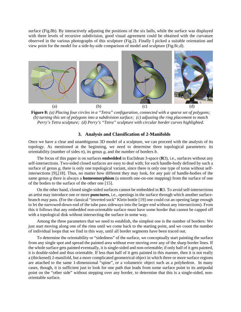
surface (Fig.8b). By interactively adjusting the positions of the six balls, while the surface was displayed with three levels of recursive subdivision, good visual agreement could be obtained with the curvature observed in the various photographs of this sculpture (Fig.2). Finally I picked a suitable orientation and view point for the model for a side-by-side comparison of model and sculpture (Fig.8c,d).

(a) (b) (c) (d)

Figure 8: (a) Placing four circles in a “Tetra” configuration, connected with a sparse set of polygons; (b) turning this set of polygons into a subdivision surface; (c) adjusting the ring placement to match

Perry’s Tetra sculpture; (d) Perry’s “Tetra” sculpture with circular border curves highlighted.

3. Analysis and Classification of 2-Manifolds Once we have a clear and unambiguous 3D model of a sculpture, we can proceed with the analysis of its topology. As mentioned at the beginning, we need to determine three topological parameters: its orientability (number of sides σ), its genus g, and the number of borders b.

The focus of this paper is on surfaces embedded in Euclidean 3-space (R3), i.e., surfaces without any self-intersections. Two-sided closed surfaces are easy to deal with; for each handle-body defined by such a surface of genus g, there is only one topological variant, since there is only one type of torus without self-intersections [9],[18]. Thus, no matter how different they may look, for any pair of handle-bodies of the same genus g there is always a homeomorphism (a smooth one-on-one mapping) from the surface of one of the bodies to the surface of the other one [15].

On the other hand, closed single-sided surfaces cannot be embedded in R3. To avoid self-intersections an artist may introduce one or more punctures, i.e., openings in the surface through which another surface-branch may pass. (For the classical “inverted sock” Klein bottle [19] one could cut an opening large enough to let the narrowed-down end of the tube pass sideways into the larger end without any intersections). From this it follows that any embedded non-orientable surface must have some border that cannot be capped off with a topological disk without intersecting the surface in some way.

Among the three parameters that we need to establish, the simplest one is the number of borders: We just start moving along one of the rims until we come back to the starting point, and we count the number of individual loops that we find in this way, until all border segments have been traced out.

To determine the orientability or “sidedness” of the surface, we conceptually start painting the surface from any single spot and spread the painted area without ever moving over any of the sharp border lines. If the whole surface gets painted eventually, it is single-sided and non-orientable; if only half of it gets painted, it is double-sided and thus orientable. If less than half of it gets painted in this manner, then it is not really a (thickened) 2-manifold, but a more complicated geometrical object in which three or more surface regions are attached to the same 1-dimensional “spine”, or a volumetric object such as a polyhedron. In many cases, though, it is sufficient just to look for one path that leads from some surface point to its antipodal point on the “other side” without stepping over any border, to determine that this is a single-sided, non-orientable surface.

Determining the genus of a surface is by far the most difficult of the three tasks. But rather than trying to find directly the genus of a given surface, one may determine instead its Euler Characteristic χ. To find χ, one covers the surface with a mesh of vertices, edges, and polygonal facets. The Euler Characteristic is then given by the expression χ = V – E + F. This is an equally good invariant to classify all 2-manifolds. However, given one of the above complex pieces of art, it may be tedious and error prone to try to sketch a mesh that covers the complete 2-manifold represented by the sculpture. There is a different approach that often proves to be much simpler. The Euler Characteristic of a set of n separate disk is χ = n. Whenever we form a ribbon-shaped bridge-connection between the rims of two disks, the Euler Characteristic is reduced by 1, because the added ribbon has two edges, but only one face. This applies whenever we make an additional connection to an independent disk or between disks that are already part of our connected network. Thus we can apply this process in reverse and ask how many independent cuts c we have to make in order to “open up” the given surface until it assumes the topology of a single disk. The Euler Characteristic is then 1 – c. Thus the Euler Characteristic of a closed ribbon (Fig.1a), whether twisted or not, is zero, and for a tetrahedral frame (Fig.3b) χ = –2.

With the Euler Characteristic established, the genus of a surface is then derived with the expressions: g = 2 – χ – b for non-orientable surfaces, and g = (2 – χ – b)/2 for double-sided surfaces. It is a non-trivial task to demonstrate that these definitions are equivalent to the number of independent

closed-loop cuts that can be made without cutting a surface into disconnected pieces. Figures 9 through 13 show the results of applying the above analysis to various 2-manifold sculptures.

For the sculptures depicted and discussed above: these are the results: Perry’s Tetra (Fig.2): σ = 2, b = 4, χ = –2, g = 0; Perry’s Continuum (Fig.4): σ = 1, b = 1, χ = –5, g = 6; Hild’s Interruption (Fig.7): σ = 2, b = 2, χ = –2, g = 1; Here are some more examples: in pictures with appended analysis of the topological parameters:

(a) “Shell”

Brent Collins: σ = 1, b = 2, χ = –1, g = 1,

(b) “Dual Universe” Charles Perry: σ = 2, b = 4, χ = –2, g = 0,

(c) “Antichron” B. Grossman:

σ = 1, b = 2, χ = –4, g = 4,

(d) “Totem 1” Carlo Séquin: σ = 2, b = 2, χ = –8, g = 4,

Figure 9: Analysis of several sculptures.

(a) “Heptoroid” Brent Collins: σ = 1, b = 1,

χ = –21, g = 22,

(b) “Arabesque-XLV” Robert Longhurst:

σ = 2, b = 2, χ = 0, g = 0,

(c) “Hollow” Eva Hild:

σ = 2, b = 1, χ = –3, g = 2,

(d) “Costa in Cube” Carlo Séquin: σ = 2, b = 3, χ = –5, g = 2,

Figure 10: Analysis of a few more sculptures. For 2-manifolds that are not primarily understandable as networks of ribbons (as were the sculptures in Figure 9), and which are dominated by large contiguous surface areas (Figs. 7, 10c, 10d), it is often easier to derive the genus directly, rather than first determining the Euler characteristic. By definition, the genus does not change if border circuits are closed by inserting topological disks. If one can seal off all rims without obtaining any intersections, one has produced the orientable surface of a handle-body, and its genus can then readily be determined by counting the number of handles and/or tunnels.

Specifically in Figure 7a one can close off the red and blue openings, and the resulting shape can then readily be recognized as a simple torus. This torus would open into an annulus if cut along the green path. Similarly, for the Costa surface shown in Figure 10d, one can easily close off the 3-segment top and bottom openings. To close off the remaining equatorial rim, consisting of six segments, one should add a large bulging balloon that does not interfere with any other parts of the sculpture. If this balloon is bulging out in the bottom/backwards direction, then the resulting shape will have three tunnel entrances near the top/front, which internally join in a Y-shaped valence-3 junction. This is the hallmark of a genus-2 handle-body.

4. Surprising Topological Equivalencies

The surprising topological equivalence between Max Bill’s Tripartite Unity [2] (Fig.11a) and a sketch (Fig.11b) appearing in George Francis’ Topological Picture Book [7] has already been discussed [12][20]. Both are single-sided surfaces of genus 3 (Dyck’s surface [6]) with a single puncture. Such a surface can be formed in a generic way by grafting a Sudanese Mӧbius band [11] onto a torus (Fig.11c).

(a) (b) (c) (d) (e) Figure 11: Surfaces with the same classification: σ=1, b=1, χ = –2, g=3: (a) Bill’s Tripartite Unity [2],

(b) sketch by George Francis [7], (c) connected sum of a torus and a Sudanese Mӧbius Band [11], (d) monkey-saddle toroid [17], (e) suitably twisted Tetra-frame (Fig.5).

In a completely different approach, Sculpture Generator I [17] can also be used to create a surface with the same topological parameters (Fig.11d). An odd number of “stories” (i.e., a saddle-tunnel combination; here there is just one.) has to be used to obtain a single-sided surface. A minimal amount of twist that closes the toroid smoothly will typically lead to a single border curve of maximal length; the branch factor for the saddles is set so as to obtain the desired Euler Characteristic. Alternatively, Perry’s Tetra can also be turned into the same topological object if the twisting of the ribbons is chosen in the right combination: exactly three of them need to make an odd number of half-flips (Fig.11e).

Next I want to explore what surfaces are single-sided and single-bordered but have a genus g = 4. The Minimal Trefoil (Fig.12a) belongs into this family; and again the Sculpture Generator I can be employed to create a corresponding surface with just a single saddle (Fig.12b). This type of surface is topologically equivalent to a connected sum of 2 Klein bottles; we can create an embedding of this surface by letting both cross handles pass through the one opening created by the single border (Fig.12c). Rinus Roelofs has created an elegant embedding of this topology class by cutting open a torus and appropriately twisting the remaining connecting ribbons so that a single border curve is formed (Fig.12d).

(a) (b) (c) (d)

Figure 12: Surfaces with classification: σ=1, b=1, χ = –3, g=4: (a) Séquin’s Minimal Trefoil [17]; (b) 4th-order-saddle toroid [17]; (c) connected sum of 2 Klein bottles; (d) Roelofs’ Mӧbius Torus [16].

Now let’s look at a family of sculptures representing an orientable surface. All of the objects in Figure 13 are topologically equivalent to a sphere with four punctures! Perry’s Tetra and also his sculpture D2d [13] belong into this family. The bamboo basket [21] by Shoryu (Fig.13b) is more difficult to analyze when just looking at pictures. When looking at the physical 3D basket, it becomes readily apparent, because of the symmetry in this object, that the result of closing the four openings will be a severely deformed sphere. Again, Sculpture Generator 1 can be used to tailor-make an object with the right topology; now we use two stories (an even number) to obtain an orientable surface, and the two saddles need to be of the ordinary biped type to result in the right genus (Fig.13c). The simplest version of a surface of this type is a disk with 3 holes; but the 3 struts between each pair of holes can be looped through the opposite hole to make a more intriguing structure (Fig.13d).

(a) (b) (c) (d)

Figure 13: Surfaces with the same classification: σ=2, b=4, χ = –2, g=0: (a) Perry’s “D2d” [13]; (b) bamboo basket by Shoryu [21]; (c) 2-story twisted toroid; (d) 3-hole button − entangled version.

5. Conclusions Trying to figure out the topological classification of many intriguing 2-manifold sculptures forced me to take a much more focused look at whatever images I could get access to. A major task was to form a mental 3D image of these shapes and then capture these geometries in some parameterized description that would allow me to fine-tune them to get as close a match as possible − yet, at the same time, to maintain the freedom to change the sculpture in some significant way. In the case of Hild’s geometries, this may be mostly a change of proportions between different funnels and tunnels, or a modification in the voluptuousness by which a dominant border would flare out. In the more ribbon-like surfaces created by Perry, I could modify the twist of individual ribbons, an operation that may affect the number of borders as well as the orientability of the surface.

The topological classification that this paper is focused on, is the coarsest way in which 2-manifolds can be analyzed. By this measure Figures 5a and 5b both belong into the same topological family. One way to distinguish them would be to analyze the interlinking of the various border loops; 5a shows no interlinking at all, while in 5b four of the possible six border pairs are linked. In general we find a strong tendency to exhibit linked border curves in Perry’s sculptures. On the other hand, Hild’s creations may have very long and complicated borders, but they are rarely interlinked.

Focusing on the border loops, another interesting question to ask is whether, in any particular sculpture with more than one border, all of them are “equivalent” in the sense that for each pair of borders there exists a homeomorphism that maps the surface back onto itself and also maps the selected two borders onto one another [5]. These issues are ongoing work and will be the subject of a future publication.

References

[1] M. Bill, Endless Ribbon (1953-56). – Middelheim Open Air Museum for Sculpture, Antwerp. [2] M. Bill, Tripartite Unity (1948-49). – http://www.lacma.org/beyondgeometry/artworks1.html [3] B. Collins, Heptoroid (1998). – http://bridgesmathart.org/bcollins/gallery6.html [4] E. Catmull and J. Clark. Recursively generated B-spline surfaces on arbitrary topological meshes. Computer-

Aided Design 10 (1978), pp 350-355. [5] W. Cavendish and J. H. Conway, Symmetrically Bordered Surfaces. Math Monthly 117 (2010). [6] W. Dyck, Beiträge zur Analysis situs. I, Math. Ann. 37 (1888) no.2, pp 457–512. [7] G. K. Francis, A Topological Picturebook. Springer, New York, 1987, p 101, fig. 33. [8] G. K. Francis and J. R. Weeks, Conway’s zip proof, Amer. Math. Monthly 106 (1999) pp 393–399. [9] J. Hass and J. Hughes, Immersions of Surfaces in 3-Manifolds. Topology 24 (1985) no.1, pp 97-112. [10] E. Hild, Homepage. – http://evahild.com/# [11] D. Lerner and D. Asimov, The Sudanese Mobius Band. SIGGRAPH Electronic Theatre, 1984. [12] T. Marar, Projective planes and Tripartite Unity. – http://www.mi.sanu.ac.rs/vismath/marar/ton_marar.html [13] C. Perry, Topological sculpture – http://www.charlesperry.com/sculpture/style/topological/ [14] C. Perry, Sculpture List. – http://www.charlesperry.com/sculpture/list/ [15] U. Pinkall, Regular homotopy classes of immersed surfaces, Topology 24 (1985) pp 421–434. [16] R. Roelofs, Mobius Torus. – http://www.rinusroelofs.nl/rhinoceros/rhinoceros-m13.html [17] C. H. Séquin, Sculpture Generator I. – http://www.cs.berkeley.edu/~sequin/GEN/Sculpture%20Generator/bin/ [18] C. H. Séquin, Tori Story. Bridges Conf. Proc., pp 121-130, Coimbra, Portugal, July 27-31, 2011. [19] C. H. Séquin, From Moebius Bands to Klein-Knottles. Bridges Conf. Proc., pp 93-102, Towson, July 2012. [20] C. H. Séquin, Cross-Caps – Boy Caps – Boy Cups. Bridges Conf. Proc., pp 207-216, Enschede, the

Netherlands, July 26-31, 2013. [21] H. Shoryu, Galaxy; Bamboo Basket (2001). Museum of Asian Art, San Francisco (Exhibit 2014). [22] J. Smith, SLIDE design environment. (2003). – http://www.cs.berkeley.edu/~ug/slide/