Embed Size (px)
Citation preview
Eindhoven University of TechnologyDepartment of Mathematics and Computer Science
Master’s thesis
Bridging SQL and NoSQL
May 11, 2012
Author: John [email protected]
Supervisor and tutor: Dr. G.H.L. [email protected]
Assessment committee: Dr. T.G.K. CaldersDr. G.H.L. FletcherDr. A. Serebrenik

Abstract
A recent trend towards the use of non-relational NoSQL databases raises the question where to storeapplication data when part of it is perfectly relational. Dividing data over separate SQL and NoSQLdatabases implies manual work to manage multiple data sources. We bridge this gap between SQLand NoSQL via an abstraction layer over both databases that behaves as a single database. Wetransform the NoSQL data to a triple format and incorporate these triples in the SQL database as avirtual relation. Via a series of self joins the original NoSQL data can be reconstructed from thistriple relation. To avoid the tedious task of writing the self joins manually for each query, we developan extension to SQL that includes a NoSQL query pattern in the query. This pattern describesconditions on the NoSQL data and lets the rest of the SQL query refer to the corresponding NoSQLdata via variable bindings. The user query can automatically be translated to an equivalent pure SQLquery that uses multiple copies of the triple relation and automatically adds the corresponding joinconditions. We describe a naive translation, where for each key-value pair from the NoSQL querypattern a new triple relation copy is used, and present several optimization strategies that focus onreducing the number of triples that must be shipped to the SQL database. We implement a prototypeof the developed theoretical framework using PostgreSQL and MongoDB for an extensive empiricalanalysis in which we investigate the impact of the translation optimizations and identify bottlenecks.The empirical analysis shows that a practical prototype based on the constructed, non-trivial, andgenerically applicable theoretical framework is possible and that we have developed a hybrid systemto access SQL and NoSQL data via an intermediate triple representation of the data, though therestill is enough space for future improvement.
iii

Acknowledgments
This thesis is the result of my master project, which completes my master Computer Science andEngineering at the Eindhoven University of Technology. The project was done within the Databasesand Hypermedia group of the department of Mathematics and Computer Science, and carried outexternally at KlapperCompany B.V., the company that introduced me to the problem and offeredresources to perform the project.
I would like to take this opportunity to thank a few people for their support during my project. Firstof all, I would like to thank my supervisor, George Fletcher, for his support and guidance during theproject and for offering the possibility to work on my suggested research topic.
Furthermore, I thank all involved employees at KlapperCompany B.V. for offering access to theirresources required to carry out my project in the form of a dataset, hardware, a pleasant workingenvironment, and general expertise regarding the project context.
Finally, thanks go out to my family, girlfriend, and friends, for their support and understanding duringmy project. Particularly in the periods of social isolation to meet an impending deadline.
John Roijackers
v

Contents
1 Introduction 11.1 Motivation . . . . . . . . . . . . . . . . . . . . . . . . . . . . . . . . . . . . . . . . . . . 1
1.1.1 Problem origin . . . . . . . . . . . . . . . . . . . . . . . . . . . . . . . . . . . . 11.1.2 Gap between SQL and NoSQL . . . . . . . . . . . . . . . . . . . . . . . . . . . 21.1.3 Real life situation . . . . . . . . . . . . . . . . . . . . . . . . . . . . . . . . . . . 3
1.2 Problem statement . . . . . . . . . . . . . . . . . . . . . . . . . . . . . . . . . . . . . . 31.3 Summary and thesis overview . . . . . . . . . . . . . . . . . . . . . . . . . . . . . . . . 4
2 Problem context 72.1 General direction . . . . . . . . . . . . . . . . . . . . . . . . . . . . . . . . . . . . . . . 7
2.1.1 Hybrid database . . . . . . . . . . . . . . . . . . . . . . . . . . . . . . . . . . . 72.1.2 Approach . . . . . . . . . . . . . . . . . . . . . . . . . . . . . . . . . . . . . . . 82.1.3 NoSQL representation . . . . . . . . . . . . . . . . . . . . . . . . . . . . . . . . 92.1.4 Data reconstruction . . . . . . . . . . . . . . . . . . . . . . . . . . . . . . . . . 11
2.2 Literature review . . . . . . . . . . . . . . . . . . . . . . . . . . . . . . . . . . . . . . . 122.3 Summary . . . . . . . . . . . . . . . . . . . . . . . . . . . . . . . . . . . . . . . . . . . 13
3 Theoretical framework for bridging SQL and NoSQL 153.1 Data incorporation . . . . . . . . . . . . . . . . . . . . . . . . . . . . . . . . . . . . . . 15
3.1.1 Availability of NoSQL data in SQL . . . . . . . . . . . . . . . . . . . . . . . . . 153.1.2 Transformation of NoSQL data to triples . . . . . . . . . . . . . . . . . . . . . . 16
3.2 Query language . . . . . . . . . . . . . . . . . . . . . . . . . . . . . . . . . . . . . . . . 183.2.1 Main idea . . . . . . . . . . . . . . . . . . . . . . . . . . . . . . . . . . . . . . . 183.2.2 Syntax description . . . . . . . . . . . . . . . . . . . . . . . . . . . . . . . . . . 193.2.3 Collaboration with SQL . . . . . . . . . . . . . . . . . . . . . . . . . . . . . . . 21
3.3 Architectural overview . . . . . . . . . . . . . . . . . . . . . . . . . . . . . . . . . . . . 213.4 Summary . . . . . . . . . . . . . . . . . . . . . . . . . . . . . . . . . . . . . . . . . . . 22
4 Query processing strategies 254.1 Base implementation . . . . . . . . . . . . . . . . . . . . . . . . . . . . . . . . . . . . . 25
4.1.1 Notation . . . . . . . . . . . . . . . . . . . . . . . . . . . . . . . . . . . . . . . . 264.1.2 Translation . . . . . . . . . . . . . . . . . . . . . . . . . . . . . . . . . . . . . . 274.1.3 Selection pushdown . . . . . . . . . . . . . . . . . . . . . . . . . . . . . . . . . . 29
vii
4.1.4 Combined selection pushdown . . . . . . . . . . . . . . . . . . . . . . . . . . . . 314.1.5 Condition derivation . . . . . . . . . . . . . . . . . . . . . . . . . . . . . . . . . 324.1.6 Transitive condition derivation . . . . . . . . . . . . . . . . . . . . . . . . . . . 33
4.2 Projection pushdown . . . . . . . . . . . . . . . . . . . . . . . . . . . . . . . . . . . . . 334.3 Data retrieval reduction . . . . . . . . . . . . . . . . . . . . . . . . . . . . . . . . . . . 34
4.3.1 General idea . . . . . . . . . . . . . . . . . . . . . . . . . . . . . . . . . . . . . 354.3.2 Triple reduction . . . . . . . . . . . . . . . . . . . . . . . . . . . . . . . . . . . . 36
4.4 Summary . . . . . . . . . . . . . . . . . . . . . . . . . . . . . . . . . . . . . . . . . . . 36
5 Experimental framework 395.1 Software . . . . . . . . . . . . . . . . . . . . . . . . . . . . . . . . . . . . . . . . . . . . 39
5.1.1 SQL . . . . . . . . . . . . . . . . . . . . . . . . . . . . . . . . . . . . . . . . . . 405.1.2 NoSQL . . . . . . . . . . . . . . . . . . . . . . . . . . . . . . . . . . . . . . . . 40
5.2 Hardware . . . . . . . . . . . . . . . . . . . . . . . . . . . . . . . . . . . . . . . . . . . 415.3 Data . . . . . . . . . . . . . . . . . . . . . . . . . . . . . . . . . . . . . . . . . . . . . . 41
5.3.1 Products . . . . . . . . . . . . . . . . . . . . . . . . . . . . . . . . . . . . . . . 415.3.2 Tweets . . . . . . . . . . . . . . . . . . . . . . . . . . . . . . . . . . . . . . . . . 43
5.4 Queries . . . . . . . . . . . . . . . . . . . . . . . . . . . . . . . . . . . . . . . . . . . . 445.4.1 Flow classes . . . . . . . . . . . . . . . . . . . . . . . . . . . . . . . . . . . . . . 445.4.2 Query types . . . . . . . . . . . . . . . . . . . . . . . . . . . . . . . . . . . . . . 455.4.3 Query construction . . . . . . . . . . . . . . . . . . . . . . . . . . . . . . . . . . 46
5.5 Triple relation implementation . . . . . . . . . . . . . . . . . . . . . . . . . . . . . . . 465.5.1 Table functions . . . . . . . . . . . . . . . . . . . . . . . . . . . . . . . . . . . . 465.5.2 Foreign data wrappers . . . . . . . . . . . . . . . . . . . . . . . . . . . . . . . . 475.5.3 Multicorn . . . . . . . . . . . . . . . . . . . . . . . . . . . . . . . . . . . . . . . 49
5.6 Setup . . . . . . . . . . . . . . . . . . . . . . . . . . . . . . . . . . . . . . . . . . . . . 505.6.1 Translation implementation . . . . . . . . . . . . . . . . . . . . . . . . . . . . . 505.6.2 Details . . . . . . . . . . . . . . . . . . . . . . . . . . . . . . . . . . . . . . . . . 51
5.7 Summary . . . . . . . . . . . . . . . . . . . . . . . . . . . . . . . . . . . . . . . . . . . 52
6 Empirical analysis 556.1 Result overview . . . . . . . . . . . . . . . . . . . . . . . . . . . . . . . . . . . . . . . . 556.2 Base implementation . . . . . . . . . . . . . . . . . . . . . . . . . . . . . . . . . . . . . 576.3 Projection pushdown . . . . . . . . . . . . . . . . . . . . . . . . . . . . . . . . . . . . . 596.4 Data retrieval reduction . . . . . . . . . . . . . . . . . . . . . . . . . . . . . . . . . . . 596.5 Increasing the NoSQL data limit . . . . . . . . . . . . . . . . . . . . . . . . . . . . . . 626.6 Summary . . . . . . . . . . . . . . . . . . . . . . . . . . . . . . . . . . . . . . . . . . . 64
7 Conclusions 657.1 Summary of theoretical results . . . . . . . . . . . . . . . . . . . . . . . . . . . . . . . 657.2 Summary of practical results . . . . . . . . . . . . . . . . . . . . . . . . . . . . . . . . 667.3 Future work . . . . . . . . . . . . . . . . . . . . . . . . . . . . . . . . . . . . . . . . . . 67
7.3.1 Nested join reduction . . . . . . . . . . . . . . . . . . . . . . . . . . . . . . . . . 677.3.2 Tuple reconstruction . . . . . . . . . . . . . . . . . . . . . . . . . . . . . . . . . 687.3.3 Triple relation reuse . . . . . . . . . . . . . . . . . . . . . . . . . . . . . . . . . 697.3.4 Dynamic run-time query evaluation strategies . . . . . . . . . . . . . . . . . . . 707.3.5 NoSQL query language standardization . . . . . . . . . . . . . . . . . . . . . . 70
A Query templates 73A.1 Product queries . . . . . . . . . . . . . . . . . . . . . . . . . . . . . . . . . . . . . . . . 73
viii

A.2 Tweet queries . . . . . . . . . . . . . . . . . . . . . . . . . . . . . . . . . . . . . . . . . 79
B Foreign data wrapper 87
Bibliography 89
ix

1Introduction
In this thesis we bring traditional relational databases and non-relational data storage closer togetherby reducing the developer’s effort required to combine data from both types of databases. This ismotivated by the recent trend to use non-relational data storage, which leads to separate databases fora single application and the consequential extra work involved with managing multiple data sources. Inthis chapter we further introduce and motivate the problem covered in this report. Firstly, Section 1.1explains the origin of the topic and motivates why it is both a theoretical and a practical problem.Section 1.2 summarizes the introduced problem and provides a list of tasks to be performed in orderto create a working solution. Finally, we provide an overview of the contents of the rest of this reportand a brief summary of the achieved results in Section 1.3.
1.1 Motivation
Before diving into the exact problem specification, this section introduces the problem and motivateswhy the topic is worth investigating. Firstly, we discuss the origin of the problem in Section 1.1.1and explain which developments have led to the existence of the problem. In Section 1.1.2 we thentheoretically describe the problem itself and why this should be solved. Finally, Section 1.1.3 describesa practical situation which indicates that it is not only a theoretical problem, but that there is acommercial need to overcome this problem as well.
1.1.1 Problem origin
Although many different types of database systems exist for decades, the relational database is themost famous database system. These relational database systems are developed, used, and optimizedfor decades and offer a solid solution for data storage in many different areas. Especially in the area ofweb applications, where the relational database used to be the standard database system for almostevery application.
Only recently a new trend is spotted in web development communities. Besides the traditionalrelational databases like MySQL, PostgreSQL, and Microsoft SQL Server that are commonlyused for websites, developers start considering alternative types of database systems for their datastorage. Products like CouchDB, MongoDB, Neo4j, Apache Cassandra, memcached, Redis,JADE, and Apache Hadoop are encountered more often in the context of web development. Instead
1
CHAPTER 1. INTRODUCTION
of conventional relational databases, these are document stores, graph databases, key-value stores,object databases, and tabular data storage systems.
The mentioned products are so-called NoSQL data storage systems, in the sense that relationaldatabases are referred to as traditional SQL systems and the alternatives are not relational databases.In the remainder of this report we adopt this naming and talk about SQL and NoSQL databasesystems as defined by Definition 1.1 and Definition 1.2.
Definition 1.1 An SQL database is a traditional relational database which can be queried using SQL.
Definition 1.2 A NoSQL database is a database that is not an SQL database. Data is not stored inrelations and the main query language to retrieve data is not SQL.
1.1.2 Gap between SQL and NoSQL
As a result of these new storage possibilities, developers investigate the available alternatives andNoSQL solutions become more commonplace. Frameworks and programming languages includesupport for these data storage alternatives and the usage of NoSQL databases increases. Partlybecause NoSQL solutions are better suited to store some types of data, but also because NoSQL hasbecome a buzzword and developers want to be part of this new hype.
This switch to NoSQL storage does however come with a major disadvantage. Decades of research inthe area of SQL databases and the resulting performance optimizations are left behind for a switch torelatively immature replacements. There are enough situations in which NoSQL products are theright tool for the job, but many software functionality can be perfectly modeled in terms of relationalentities and is well-suited for traditional SQL data storage.
Problems arise when a single software product requires data storage where a part of the data is ideallystored in a NoSQL database, whereas the rest of the data is perfectly relational and thus well-suitedfor a traditional SQL database. This raises the question what type of data storage must be chosen forthe application. As different parts of the data are well-suited for different types of databases, choosingone type of data storage always implies that a part of the data is stored in a less appropriate way.
The obvious compromise is a solution where the relational part of the data is stored in an SQLdatabase, while the non-relational data is stored in NoSQL. However, this creates a challenge forscenarios where data from both sources is required. Queries that have to combine data from bothdata sources require extra programming to combine the data and present the correct result.
Another drawback of separating the data storage is that the developers need to access differentdatabase systems. Each database has its strengths, weaknesses, and query syntax. Currently, thereis no standard for NoSQL query languages. Moreover, because NoSQL is a collective noun for avariety of storage types it is doubtful whether it is even possible to create a single query language. Ingeneral, using multiple database systems will increase the complexity and reduce maintainability ofthe application.
Separating relational and non-relational data in SQL and NoSQL databases respectively certainlyhas advantages. It is however not straightforward to put this into practice without any substantialdrawbacks. Bridging the gap between SQL and NoSQL therefore is an interesting research topic andovercoming the mentioned drawbacks would allow developers to use the right storage solution for bothparts of data they have to manage.
2
1.2. PROBLEM STATEMENT
1.1.3 Real life situation
We came across a company that is facing exactly the problem described in Section 1.1.2. Thetechnological core of the companies activities concerns managing a large collection with different typesof products. These products have different suppliers and often do not have the same set of attributesassigned. Also, the products get revised periodically. In this case the product itself remains the same,but only the newest version of the product can be ordered by customers. These revisions can cause achange in the set of attributes of the product. This implies that the set of attributes of a product isnot fixed, which means that using a schemaless NoSQL database for the product data can be moreconvenient than fitting it in an SQL database.
Besides the product information, the company has to store other data related to their daily activities.This mainly is information regarding customers, orders, suppliers, and invoices. This information canbe summarized as CRM data, which is relational data and thus, in contrast to the product data,perfectly suited for an SQL database. Note that this situation matches the general theoretical problemdescribed before. Different parts of the data are well-suited for different types of storage solutions.
As also proposed in Section 1.1.2, the company decided to split the data and use both an SQL and aNoSQL solution to store the CRM data and the product information respectively. As a result ofthis decision developers now need to retrieve data from different data sources in order to implementcertain functionality, for example to generate invoices containing product information. Though this isnot an insurmountable problem, it has some disadvantages for the developers. Besides the fact thatthis requires knowledge of both database systems, the data from both sources has to be manuallymerged in each situation where combined information is needed.
This raises the question if the problem of combining data from different data sources can be solvedin another way, such that developers are not bothered with different data sources and can retrieveinformation as if it they access only a single data storage system. In other words, is it possible tofind a solution that bridges the gap between SQL and NoSQL by combining them such that thedisadvantages of different data storage systems are eliminated. The company’s desire to combinedifferent database systems in a single application indicates that the previously described problem isnot just a theoretical one, but that there is an actual practical need to find a solution for bridging thegap between SQL and NoSQL.
Note that we do not describe the company in much detail and only mention the technological aspectsof the problem. Although the aim of this project is to cover the topic generically such that ideas,suggestions, or solutions are universally applicable, the company’s specific situation is sometimes usedas a guideline in this report. This implies that some decisions are based on the practical applicationin the company’s situation. References to ‘the company’ in this report aim to point at the situationdescribed in this section. Also, the company cooperates in the project by offering access to theirhardware, data, and expertise.
1.2 Problem statement
Section 1.1 introduced the topic of this report and explains how the problem has arisen, why there isa theoretical need to solve it, and that there are companies currently coping with this problem. Inthis section we try to formulate the exact problem statement and then list the subproblems discussedin the following chapters.
Splitting application data into different database systems has advantages, but also introduces seriousdisadvantages which we have to overcome. Most of the disadvantages are a result of the fact that
3
CHAPTER 1. INTRODUCTION
splitting the data also enforces developers to retrieve data from different sources. We attempt toprovide a solution such that the benefits of separate data storage systems remain, while the introducedproblems are mostly eliminated.
Problem statement Dividing application data over SQL and NoSQL storage generates a gap interms of uniform data access. Currently, no solutions are available to bridge this gap by masking theunderlying data separation and taking over the task of managing multiple data sources.
This problem statement naturally implies the project goal to bridge this gap between SQL andNoSQL. Because bridging the gap is not a trivial task, we outline the context of our problem andfocus on a specific set of tasks that together provide a solution to the stated problem. Together thesetasks provide a brief overview of the approach we take and a breakdown of how we achieve this goal.
Task 1 Construct a theoretical framework to bridge SQL and NoSQL
Determining which approach to take and what our general solution should look like is the first steptowards our ultimate goal. The theoretical framework should describe how we model the data, whatimplications this has for developers, and give an architectural overview of how we want to genericallybridge SQL and NoSQL.
Task 2 Provide a formal definition to specify the developed theoretical framework
The theoretical framework is specified in more detail and formalized. Like the theoretical framework,the formalization should result in a generic solution applicable to arbitrary SQL and NoSQL databases.Therefore, this formalization should be given in a database independent formal language.
Task 3 Create a prototype implementation of the theoretical framework
To verify that our theoretical solution is feasible in practice we want to implement a prototype thatdemonstrates that the proposal can actually be implemented and that the framework can be efficientlyapplied in a commercial environment.
Task 4 Conduct a thorough experiment with the prototype and analyze the results
The experiment is used to empirically analyze the performance of the prototype. Furthermore, wewant to use the experiment results to indicate possible bottlenecks in the prototype and use thisinformation for further improvement of the implementation.
1.3 Summary and thesis overview
This report is an exposition of the work we did in an attempt to bring SQL and NoSQL closertogether. The recent trend towards using NoSQL databases for application data raises the questionwhere to store which part of the data. Separating the data and storing one part in an SQL databaseand the other part in a more suitable NoSQL database implies extra work for software developerswho then have to manage multiple data sources. Tackling this problem is moreover motivated bya company that encountered this exact problem, which indicates that there is a practical need tobring SQL and NoSQL closer together. We want to bridge this gap between SQL and NoSQL byproposing a solution to this data separation problem.
4
1.3. SUMMARY AND THESIS OVERVIEW
The tasks defined in Section 1.2 are a guideline for this report. Every task has its own chapterdedicated to it, in which we elaborate on the exact problem and describe our proposed way to solveit. This section gives a brief overview of the contents of the report at chapter level and succinctlysummarizes the main topic of each chapter.
Firstly, Chapter 2 defines the problem context. Combining SQL and NoSQL is a relatively newresearch area. Therefore, we describe the general direction we choose to solve the problem, list somealternative approaches, and explore the available literature related to the problem topic. This chapterelucidates our choice to represent NoSQL data as triples and explains how the NoSQL data can bereconstructed from these triples.
Chapter 3 describes the theoretical framework we propose. This includes details about the imple-mentation at a functional level and gives an overview of the framework architecture. This chapteranswers Task 1 by introducing the availability of relation F containing the NoSQL triples in therelational database. Furthermore, we present a query language that allows developers to access bothdata sources in a single statement.
We formalize this theoretical framework using relational algebra in Chapter 4, thereby addressingTask 2. The solution provided in this chapter offers a generic solution for bridging SQL and NoSQL,regardless of which data storage solutions are used. As part of this formal query translation we includesome optimization strategies to optimize the performance of our solution.
Next, Chapter 5 focuses on Task 3 and describes how the formally defined framework is implemented.This also includes the experiment setup, which is required to analyze the performance of the prototype.In this chapter we can no longer talk about SQL and NoSQL in general, but choose specific softwareproducts. Our implementation uses PostgreSQL as a relational database. Non-relational data isstored in MongoDB, which is a prototypical example of a NoSQL system. Both software choices aremotivated and further implementation details are described as well.
The prototype is used for an experiment to compare the performance between different implementationsof the proposed framework. The results are analyzed in Chapter 6, following Task 4. This analysisshows that our prototype is an acceptable solution to bridge the gap between SQL and NoSQL, butthat there also is space for further improvements.
Lastly, we give an overview of what we have achieved in Chapter 7. We summarize the conclusions thatcan be derived from the work we did and offer suggestions for future work not covered in this report.These suggestions can be the next steps to improve the developed prototype towards a commercialstrength hybrid SQL-NoSQL database.
5

2Problem context
In the previous chapter we have indicated the problem introduced by the movement towards NoSQLdata storage. Ideally we want to store each part of the application data in a type of database designedand suited for that specific type of data. This allows to fully benefit from the advantages the databaseoffers. However, separating application data over multiple databases implies that the data is splitand this introduces use cases in which data from both sources has to be combined. Ideally, we donot want to bother the developer with this task and provide a solution which hides the underlyingseparated data storage to the developer. The solution for this problem can be searched for in manydifferent directions. We therefore first describe what type of approach we want to take in this report inSection 2.1. This includes how the data is handled and how the hybrid result can be obtained by thedeveloper. After we have determined our main solution direction, we search the available literaturerelated to our intended approach. In Section 2.2 we discuss the relevant literature found and sketchan overview of the work done related to our problem. Finally, Section 2.3 summarizes how we want totackle the data separation problem and gives an overview of the work currently done by others relatedto this topic.
2.1 General direction
Before we study the available literature to investigate what work has been done or can be used tocombine relational and non-relational data, we first outline the project context. We can search fora solution to combining data from multiple databases in different directions. In Section 2.1.1 wetherefore begin with an explanation of which general direction we choose to use and describe how anideal hybrid database would be modeled. Subsequently, we zoom in on the chosen direction and specifyour intended approach in more detail in Section 2.1.2 by motivating our decision to include NoSQLdata as a relation in the SQL database. Section 2.1.3 then explains how we model the NoSQL dataas triples, such that they can be represented as a relation in SQL. How the NoSQL triples can beused to reconstruct the non-relational data is described in Section 2.1.4.
2.1.1 Hybrid database
Most of the problems that occur when storing a part of your data in an SQL database and the otherpart in a NoSQL database are based on the fact that the data has to be retrieved from differentsources. Multiple data sources means multiple technologies a developer must be able to work with in
7
CHAPTER 2. PROBLEM CONTEXT
order to access all data, multiple query languages, and multiple parts of your code dedicated to dataretrieval. Moreover, an additional piece of code responsible for combining the data from both sourcesagain is needed to construct the final result.
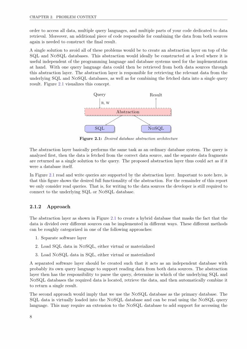
A single solution to avoid all of these problems would be to create an abstraction layer on top of theSQL and NoSQL databases. This abstraction would ideally be constructed at a level where it isuseful independent of the programming language and database systems used for the implementationat hand. With one query language data could then be retrieved from both data sources throughthis abstraction layer. The abstraction layer is responsible for retrieving the relevant data from theunderlying SQL and NoSQL databases, as well as for combining the fetched data into a single queryresult. Figure 2.1 visualizes this concept.
Abstraction
Query Result
SQL NoSQL
R, W
Figure 2.1: Desired database abstraction architecture
The abstraction layer basically performs the same task as an ordinary database system. The query isanalyzed first, then the data is fetched from the correct data source, and the separate data fragmentsare returned as a single solution to the query. The proposed abstraction layer thus could act as if itwere a database itself.
In Figure 2.1 read and write queries are supported by the abstraction layer. Important to note here, isthat this figure shows the desired full functionality of the abstraction. For the remainder of this reportwe only consider read queries. That is, for writing to the data sources the developer is still required toconnect to the underlying SQL or NoSQL database.
2.1.2 Approach
The abstraction layer as shown in Figure 2.1 to create a hybrid database that masks the fact that thedata is divided over different sources can be implemented in different ways. These different methodscan be roughly categorized in one of the following approaches:
1. Separate software layer
2. Load SQL data in NoSQL, either virtual or materialized
3. Load NoSQL data in SQL, either virtual or materialized
A separated software layer should be created such that it acts as an independent database withprobably its own query language to support reading data from both data sources. The abstractionlayer then has the responsibility to parse the query, determine in which of the underlying SQL andNoSQL databases the required data is located, retrieve the data, and then automatically combine itto return a single result.
The second approach would imply that we use the NoSQL database as the primary database. TheSQL data is virtually loaded into the NoSQL database and can be read using the NoSQL querylanguage. This may require an extension to the NoSQL database to add support for accessing the
8
2.1. GENERAL DIRECTION
SQL data. Depending on the specific SQL and NoSQL solutions, transforming structured SQL datato fit in an unstructured NoSQL database should be relatively easy. Most NoSQL products aredesigned to store schemaless data, and fitting in structured, relational data therefore means movingthe data to a less constrained environment.
Another approach is to incorporate the NoSQL data in the relational database. This incorporationis not necessarily achieved by materializing the NoSQL data in the relational database. It can alsobe an implementation that makes the NoSQL data virtually available and thus does not actuallyretrieve the NoSQL data until query execution. Similar to the previous approach this means that thedeveloper opens a connection to the SQL database, and can then also read the NoSQL data. Themost obvious challenge with this approach is how to represent the unstructured NoSQL data in anSQL database, and thereafter allow the developer to easily construct queries that read data from theNoSQL data source.
On the other hand, using the SQL database as the primary data storage system and including theNoSQL data has important advantages. Firstly, relational databases and SQL are an establishedstandard regarding data storage. In general, it is safe to say that an arbitrary professional softwareengineer knows SQL and probably even has experience constructing queries. The familiarity withrelational databases and SQL in particular make the relational database a good candidate to serve asthe main system for a hybrid database, especially with respect to the ease of adoption.
Furthermore, relational databases are used, researched, and optimized for decades. Not only arerelational databases well-known, they also have proven to be a mature solution for data storage.Maturity of SQL databases can be viewed in different perspectives. Besides aspects like performanceand stability, many relational databases are also easily extensible. Many SQL databases offer possibleways to integrate external data out of the box.
The movement to use NoSQL databases is a trend visible especially the last few years. Until recently,relational databases offered a suitable solution for data storage for most of the problems occurring insoftware development. Many data can still be perfectly stored in an SQL database, and the hypeNoSQL created causes developers to move relational data to NoSQL storage and thereby sacrificingthe advantages a relational database offers in favor of the benefit the NoSQL solution offers for asubset of the data.
In case most data can still be perfectly stored in an SQL database, using that as the primary storagesolution will reduce the number of queries that actually need to read the NoSQL data. In that case,the hybrid database is used solely as an SQL database and all advantages of relational databasesapply to that particular query. In other words, queries that only read relational data are not affectedby the abstraction layer.
Besides the advantages the third approach offers compared to the other methods, our goal is toimplement a prototype of the proposed solution. Provided the advantages, especially the extensibilityof many SQL databases, we take the third approach and focus on including NoSQL data in SQL.Either as a virtual or as a, perhaps partially, materialized view.
2.1.3 NoSQL representation
In Section 2.1.2 we motivated our intention to load NoSQL data in an SQL database. Ideally, wewant to provide a solution for creating a hybrid SQL-NoSQL database that is generically applicable,and thus independent of the underlying SQL and NoSQL databases. One of the problems of NoSQLis that there is no standard comparable to SQL for relational databases. All SQL databases can bequeried using SQL, whereas many NoSQL databases come with their own query language.
9
CHAPTER 2. PROBLEM CONTEXT
As a result of this lack of standardization there is little to no interoperability among different NoSQLsystems. Not only is this difficult for developers, who cannot easily work with different NoSQLsolutions without the need to explore the possibilities of another query language and data storagesystem, but it also causes problems for our project. The absence of an established standard for NoSQLstorage makes it difficult to provide a generic abstraction layer.
In this section we describe a triple notation to represent arbitrary data. Furthermore, we give examplesof how other data formats can be transformed to the proposed triple representation.
Different NoSQL data types assume a different data structures. Graph databases represent theirdata as a graph, key-value stores can use a hash map to store their data, whereas document orienteddatabases contain nested sets of key-value pairs. All data representations however have one thing incommon. Each part of a data entity is related to another part of that entity in a specific way.
Inspired by RDF1, we decide to represent NoSQL data as triples describing how different objects ofthe data are related to another object. RDF is standardized and a W3C recommendation. Giventwo data objects s and o, we can use a triple (s, p, o) to describe that object s has a relation p toobject o. Data objects can be constant values, but also identifiers to describe an object that has aset of properties described as relations to constant objects. To express that Bob is 37 years old, wecan use the triples {(h, name,Bob) , (h, age, 37)}. Note that we use h to combine the name and ageinformation.
Using triples provides a standard way to describe data and results in better interoperability betweendifferent NoSQL databases when the data is represented in the same way. The main advantage oftriples to represent data is the flexibility. Basically, (s, p, o)-triples can be used to describe any type ofdata. Because of this flexibility arbitrary NoSQL data and even SQL records can easily be described.Relational tables for example, can be described using triples by creating a triple (s, p, o) for each datarow attribute describing that record s has value o for attribute p.
The (s, p, o)-triples refer to the RDF specification, where the s, p, and o respectively refer to theterms subject, predicate, and object. We use the triple notation to convert non-relational data to aformat suitable to be represented as an SQL relation. This means that the p part of the triple is usedto describe an attribute name, while the o value contains the value for this attribute. The s is usedto indicate that multiple triples belong together and that they describe different attributes of thesame data entity, like the h we used in the example to describe that Bob’s age is 37. To clarify theintended use of the different triple positions for our use case, we refer to (s, p, o)-triples as (id, key,value)-triples from now on. Or abbreviated, (i , k , v)-triples.
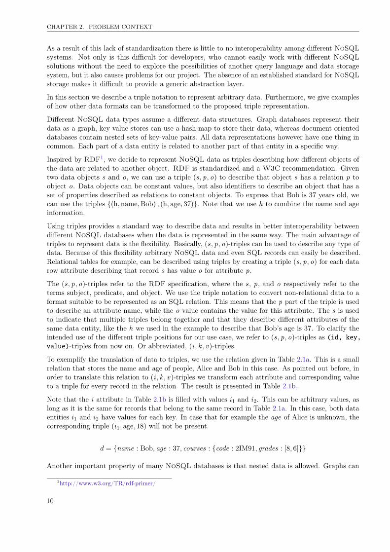
To exemplify the translation of data to triples, we use the relation given in Table 2.1a. This is a smallrelation that stores the name and age of people, Alice and Bob in this case. As pointed out before, inorder to translate this relation to (i , k , v)-triples we transform each attribute and corresponding valueto a triple for every record in the relation. The result is presented in Table 2.1b.
Note that the i attribute in Table 2.1b is filled with values i1 and i2. This can be arbitrary values, aslong as it is the same for records that belong to the same record in Table 2.1a. In this case, both dataentities i1 and i2 have values for each key. In case that for example the age of Alice is unknown, thecorresponding triple (i1, age, 18) will not be present.
d = {name : Bob, age : 37, courses : {code : 2IM91, grades : [8, 6]}}
Another important property of many NoSQL databases is that nested data is allowed. Graphs can
1http://www.w3.org/TR/rdf-primer/
10
2.1. GENERAL DIRECTION
id name age1 Alice 182 Bob 37
(a) Relational representation
id key valuei1 id 1i1 name Alicei1 age 18i2 id 2i2 name Bobi2 age 37
(b) Triple representation
Table 2.1: Example data transformation between two representations
also be considered nested data when child nodes are viewed as nested information related to theparent node. Consider the following example of a nested document d, with the corresponding triplerepresentation shown in Table 2.2.
id key valuei1 name Bobi1 age 37i1 courses i2i2 code 2IM91i2 grades i3i3 0 8i3 1 6
Table 2.2: Triple representation of nested document d
Although we have only transformed a single nested document, we have multiple values for i , theid attribute. Because document d was nested we use these different it values to show the relationbetween the different triples. The it values are only used to connect triples and are not present inthe original document d. Because this information is only used to provide information about how thetriples are connected they can have arbitrary values as long as the correct structure of d is described.This implies that this data is not stable and thus should not be used in a query for any other purposethan connecting triples.
2.1.4 Data reconstruction
Data represented as triples provides flexibility, but this comes at a price. As can be observed from theexample triple relations in Table 2.1b and Table 2.2, a single NoSQL data entity is represented inmultiple records. Moreover, there is no guarantee that the relation is sorted in any way. The recordsrelated to the same NoSQL data entity might thus be divided arbitrarily distributed over the triplerelation records. We must reconstruct the data, so that related records are combined again.
This is where the it values come in. As pointed out in Section 2.1.3, these values have no meaningexcept that they determine the structure of the data. Records with the same id value representkeys with values that belong to the same data entity, at the same nesting level. An it value for thevalue attribute in the triple table means that the attributes belonging to it are nested under the keyattribute of the record at hand.
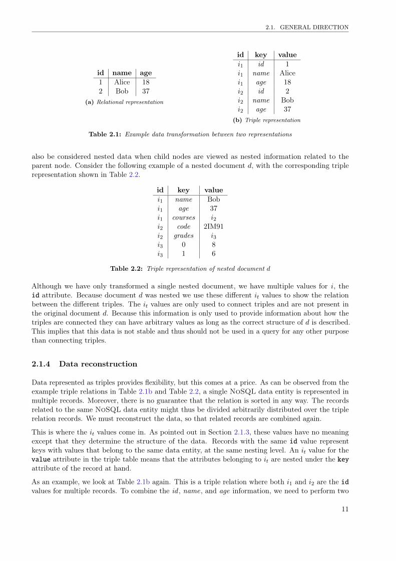
As an example, we look at Table 2.1b again. This is a triple relation where both i1 and i2 are the idvalues for multiple records. To combine the id , name, and age information, we need to perform two
11
CHAPTER 2. PROBLEM CONTEXT
consecutive self joins and ensure that the id values are equal. Let the relation as shown in Table 2.1bbe called T , then renaming and theta-joins do the trick.
T1id12
(a) One relation
T2id name1 Alice2 Bob
(b) Two relations
T3id name age1 Alice 182 Bob 37
(c) Three relations
Table 2.3: Stepwise data reconstruction example
The relations T1, T2, and T3 as shown in Table 2.3a, Table 2.3b, and Table 2.3c respectively, areconstructed using relational algebra expressions. These expressions include the renaming steps andthe appropriate theta-joins to reconstruct the data and output the original data as a single relation.Below we give the corresponding relational algebra expressions.
T1 = ρT1(id)(πvi(σki=id
(ρTi(i,ki,vi) (T )
)))T2 = ρT2(id ,name)
(πvi,vn
(σki=id∧kn=name
(ρTi(i,ki,vi) (T ) on ρTn(i,kn,vn) (T )
)))T3 = ρT3(id ,name,age)
(πvi,vn,va
(σki=id∧kn=name∧ka=age
(ρTi(i,ki,vi) (T ) on ρTn(i,kn,vn) (T ) on ρTa(i,ka,va) (T )
)))Note that relation T3 is equal to the original data as introduced in Table 2.1a. In this specific casetwo self joins suffice to reconstruct the original data entities from the triples relation T . In general, toreconstruct data with n attributes n− 1 self joins are required. The work involved to reconstruct theoriginal data from the triple representation is tedious and we have to automate this process as part ofour hybrid database solution.
2.2 Literature review
Though the NoSQL movement is relatively new and solutions to combine relational and non-relationaldata are not extensively researched, related work has been performed in the area of NoSQL andcombinations of different data types. In this section we give an overview of the current research stateof topics related to our intended goal to bring relational and non-relational data closer together.
Firstly, we focus on the discussion on NoSQL storage in available literature. A thorough survey ofavailable non-relational databases is presented in 2009 [Var09]. This includes an overview of NoSQLstorage solutions available at the time of writing and addresses the advantages and disadvantages ofnon-relational data storage. Furthermore, the question whether a NoSQL database is the correct choicegiven a dataset is discussed. Others have questioned the NoSQL hype by arguing that the problemsNoSQL solution claim to solve are not caused by the relational structure of SQL databases [Sto10].Also, overviews of both SQL and different types of NoSQL solutions are available which includeuse cases for different database types [Cat10]. Moreover, this describes the trade off that has to bemade when choosing a NoSQL solution to store data in terms of sacrificing certain desirable databaseproperties to improve others. Arguments both in favor and against NoSQL database solutions arepresent in available literature. The general conclusion however is that NoSQL storage fulfills a need,but its use should be carefully considered and decently motivated as it implies sacrificing importantproperties offered by traditional relational databases.
12
2.3. SUMMARY
In our problem case, considerations have led to the conclusion that data should be divided overdifferent database types. Our proposal to create a hybrid database, which hides the underlying dataseparation, is not new. In the early 1990’s a concept called mediators has been researched [Wie92].In this context, a mediator is an extra layer on top of your data storage which takes care of morecomplicated tasks. This includes calculations over the underlying data, data amount management,keeping track of derivable data, and accessing and merging external data. Also, incorporating NoSQLdata as a relation in an SQL database is investigated before. A recent example is the inclusion ofXML data as a relation, with a query language modified to query over this XML data [GC07].
Also, the idea of storing data as triples is literally decades old. Again in the early 1990’s it hasbeen introduced and named the first order normal form [LKK91]. The first order normal form is anormalization of the database itself. Instead of real triples, a relation is introduced with four columnsrepresenting the relation name, key, attribute name, and attribute value. This way, multiple relationscan be merged in a single relation. Without the relation name column to store from which relation thedata originates, these are in fact triples describing relational data. Other papers describe the same ideafor single relations by providing transformation functions to represent a normal, horizontal relation, toa vertical table containing the same amount of information in triple format [ASX01]. TransformingNoSQL data to triples is a specific application of the general data mapping framework, which aims atdescribing arbitrary mappings over data [FW09]. In general, these mappings do not necessarily aim atobtaining another representation, but can also be used to derive new information or combine availabledata.
Our generic NoSQL data description using triples has the disadvantage that the NoSQL data isfirst transformed to triples, and then later reconstructed again. Furthermore, the triple notationis extremely flexible, but for many data the notation is quite cumbersome and not compact. Also,querying the triple data to select data and combining corresponding triples is inefficient compared toworking with relations that already have corresponding attributes combined in a single record. Theflexibility of the triple notation however is a major advantage that can justify the associated drawbacks.Moreover, optimizing performance of triple datasets is a topic of research and some promising solutionsand indexing techniques have been proposed that can help reduce the performance penalty [FB09].
Effectively querying the NoSQL data, represented as triples, means that triples have to be manuallycombined. Previous research has led to a query language proposal that includes SPARQL queries intraditional SQL and thereby simplifies querying NoSQL data [CDES05, DS09]. Furthermore, theNoSQL part of the query can be automatically translated to an SQL equivalent by applying a semanticspreserving translation [CLF09]. Though this last suggestion is originally aimed at materialized tripledata that is actually stored in the relational database, the same ideas can be applied when we keepthe non-relational data stored on the NoSQL side and transform it to triples on the fly at queryexecution.
2.3 Summary
Most of the problems introduced when data for a single application is partially stored in SQL, andpartially in NoSQL, are a result of the fact that this implies separate data sources. A solution forthis problem, which performs the task of combining data from both databases automatically, canbe found in different directions. We choose to create an abstraction layer on top of the SQL andNoSQL databases that presents itself as a single database to the developer, thereby ideally completelyhiding the underlying separate SQL and NoSQL databases. To combine the data, we include theNoSQL data in the relational database. The main reason to choose this approach is the maturity ofSQL databases. As a result, SQL is a well-known standard that most developers already know. Also,
13
CHAPTER 2. PROBLEM CONTEXT
the SQL database can take care of the more complicated tasks such as ordering, aggregation, andgrouping.
The NoSQL data must be included as structured data in a relational database, because SQL databasesare designed to work with relations instead of schemaless data. To obtain a generically applicablesolution we represent the NoSQL data as RDF-like triples. This allows maximum flexibility and canbe used to model any type of data. Furthermore, triples are nicely structured and can thus easilybe included in an SQL database as a relation. Via a series of self joins on these triples the originalNoSQL data can be reconstructed. Because creating the self joins is a tedious task, we have to find away to automatically construct this query part with the appropriate conditions.
Our brief literature study showed that our goal to create a hybrid framework to combine SQL andNoSQL data in a single system, at least from the perspective of the developer, has been abstractlydescribed decades ago. Proposals for query languages that allow the developer to query the tripledata incorporated as a relation in an SQL database have been made. These suggestions form a goodstarting point for the design of a theoretical framework for our situation in which we want to access theexternal data on the fly, using a triple representation to provide a generically applicable solution.
14
3Theoretical framework for bridging SQL and NoSQL
The previous chapter described the abstraction layer we wish to add on top of the separated databasesto bridge the gap between SQL and NoSQL by generating a hybrid database. To achieve this, we musttransform the NoSQL data to a triple representation and incorporate these triples in the relationaldatabase. How we achieve this is explained in Section 3.1.
As mentioned in the previous chapter, reconstructing the NoSQL data in the relational database is atedious task because multiple self joins are required to achieve this. We want to automate this process,which means that we have to find a way to include the NoSQL data conditions in a query languagesuch that the developer does not have to worry about this reconstruction. In Section 3.2 we thereforespecify a query language that can be automatically translated to a pure SQL equivalent that takescare of the self joins and corresponding join conditions.
Section 3.3 then shows the architectural overview of our proposed solution. This describes the stepsinvolved during the lifetime of a single user query. A summary of the entire theoretical framework isgiven in Section 3.4. The developed theoretical framework matches the criteria to complete Task 1and serves as a basis for a prototype implementation.
3.1 Data incorporation
We use a triple representation to describe arbitrary NoSQL data. How this is incorporated in anSQL database is described in Section 3.1.1. To keep the solution generically applicable, no specificimplementation details are provided. Furthermore, in Section 3.1.2 we explain how NoSQL data canbe transformed to triples to allow the data to be accessed in the relational database.
3.1.1 Availability of NoSQL data in SQL
With the triple representation to describe NoSQL data generically as explained in Section 2.1.3,we can now further specify how the data from the NoSQL database is included in the relationaldatabase. Without going into implementation details, we assume that in SQL there is a relationF (id, key, value) available containing all triples to describe the NoSQL data we want to incorporatein the SQL database. Note that this may be a virtual relation. That is, it can be implemented as anon-materialized view on the NoSQL data.
15
CHAPTER 3. THEORETICAL FRAMEWORK FOR BRIDGING SQL AND NOSQL
For example, the following query would select all age values available in the NoSQL dataset:
ρR(age) (πvalue (σkey=age (F )))
The relation F can be used in queries like any other relation in the SQL database. This means we canjoin F to ‘normal’ relations to combine SQL and NoSQL data in a single query result. Importantto notice however, is that the records in F are retrieved from an external data source, in this case aNoSQL database. To return the records of F , the SQL database has to retrieve the external data intriple format from the NoSQL database.
This implies that the retrieved data has to be communicated to the relational database. Dependingon the exact implementation of F and the method used to retrieve data from the NoSQL source, thismight violate the atomicity of the query and consistency of the query result. Imagine an implementationof F where data is streamed from the NoSQL source at query time. When a query requires a largeamount of data to be streamed to the SQL database, for some reason the NoSQL database might notbe available. This can possibly result in an empty relation F . Or, even if the implementation functionscorrectly, as the first part of the data is being streamed, another user can modify the NoSQL datathat still has to be transmitted to SQL. Thereby possibly causing inconsistency in the total set ofNoSQL data sent to the relational database.
Furthermore, we assume that F knows to which NoSQL source it should connect and what data toretrieve. In practice the implementation of F is provided with parameters to specify how the NoSQLdatabase should be used. For readability however, we ignore these parameters and assume F returnstriples of the NoSQL source we want to access. In the remainder of this report we will thus use F asthe relation of triples that represent the NoSQL data. To include connection parameters, this cansimply be replaced with F (p1, p2, . . . , pn) in order to provide n parameters.
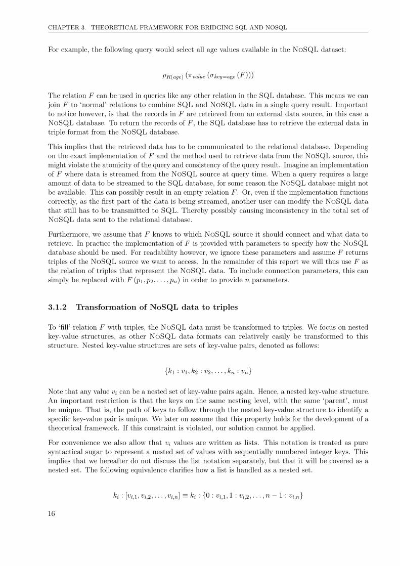
3.1.2 Transformation of NoSQL data to triples
To ‘fill’ relation F with triples, the NoSQL data must be transformed to triples. We focus on nestedkey-value structures, as other NoSQL data formats can relatively easily be transformed to thisstructure. Nested key-value structures are sets of key-value pairs, denoted as follows:
{k1 : v1, k2 : v2, . . . , kn : vn}
Note that any value vi can be a nested set of key-value pairs again. Hence, a nested key-value structure.An important restriction is that the keys on the same nesting level, with the same ‘parent’, mustbe unique. That is, the path of keys to follow through the nested key-value structure to identify aspecific key-value pair is unique. We later on assume that this property holds for the development of atheoretical framework. If this constraint is violated, our solution cannot be applied.
For convenience we also allow that vi values are written as lists. This notation is treated as puresyntactical sugar to represent a nested set of values with sequentially numbered integer keys. Thisimplies that we hereafter do not discuss the list notation separately, but that it will be covered as anested set. The following equivalence clarifies how a list is handled as a nested set.
ki : [vi,1, vi,2, . . . , vi,n] ≡ ki : {0 : vi,1, 1 : vi,2, . . . , n− 1 : vi,n}
16
3.1. DATA INCORPORATION
To translate a nested key-value structure s to triples, we have to ensure that the triples correspondingto same structure s are given the same id value. As mentioned before, the exact value of this id isnot important, as long as it is the same for triples that belong to the same NoSQL data object. Or inthis case, the same nesting level in a key-value structure s.
Nested sets of key-value pairs are recursively transformed similar to other key-value pairs, except thatthese triples get a new unique id value. To connect the triples of the parent key-value structure tothe nested one, a triple is added describing the relation using the key of the nested key-value set.
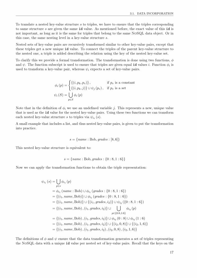
To clarify this we provide a formal transformation. The transformation is done using two functions, φand ψ. The function subscript is used to ensure that triples are given equal id values i. Function φi isused to transform a key-value pair, whereas ψi expects a set of key-value pairs.
φi (p) =
{{(i, pk, pv)} , if pv is a constant{(i, pk, j)} ∪ ψj (pv) , if pv is a set
ψi (S) =⋃p∈S
φi (p)
Note that in the definition of φi we use an undefined variable j. This represents a new, unique valuethat is used as the id value for the nested key-value pairs. Using these two functions we can transformeach nested key-value structure s to triples via ψi1 (s).
A small example that includes a list, and thus nested key-value pairs, is given to put the transformationinto practice.
s = {name : Bob, grades : [8, 6]}
This nested key-value structure is equivalent to:
s = {name : Bob, grades : {0 : 8, 1 : 6}}
Now we can apply the transformation functions to obtain the triple representation:
ψi1 (s) =⋃p∈s
φi1 (p)
= φi1 (name : Bob) ∪ φi1 (grades : {0 : 8, 1 : 6})= {(i1,name,Bob)} ∪ φi1 (grades : {0 : 8, 1 : 6})= {(i1,name,Bob)} ∪ {(i1, grades, i2)} ∪ ψi2 ({0 : 8, 1 : 6})
= {(i1,name,Bob) , (i1, grades, i2)} ∪⋃
p∈{0:8,1:6}
φi2 (p)
= {(i1,name,Bob) , (i1, grades, i2)} ∪ φi2 (0 : 8) ∪ φi2 (1 : 6)
= {(i1,name,Bob) , (i1, grades, i2)} ∪ {(i2, 0, 8)} ∪ {(i2, 1, 6)}= {(i1,name,Bob) , (i1, grades, i2) , (i2, 0, 8) , (i2, 1, 6)}
The definitions of φ and ψ ensure that the data transformation generates a set of triples representingthe NoSQL data with a unique id value per nested set of key-value pairs. Recall that the keys on the
17
CHAPTER 3. THEORETICAL FRAMEWORK FOR BRIDGING SQL AND NOSQL
same nesting level, with the same ‘parent’, must be unique. From these properties we can deducethat the combination of id and key is unique and thus unambiguously refers to a single value in theNoSQL data.
3.2 Query language
We include NoSQL data in an SQL database via a triple relation F . Using pure SQL it is possibleto request data from both the SQL and the NoSQL data source. In Section 2.1.4 we have shown therelational algebra methods required to reconstruct NoSQL data via a series of self joins on the triplerelation. A disadvantage is that the work involved to reconstruct the NoSQL data is tedious. Ideally,we would like to automate the generation of the query part to reconstruct the NoSQL data. However,this requires an extension to the query language. This section describes how SQL can be extended toallow developers to more easily manage NoSQL data in the database queries. Firstly, Section 3.2.1describes the general concept of variable binding using basic graph patterns from SPARQL. Thissyntax is modified as described in Section 3.2.2 to better fit our use case. In the same section wediscuss the advantages and disadvantages of this modified query language. Finally, in Section 3.2.3 weexplain how data originating from the NoSQL database can be used in the SQL part of the user query.Together this specifies the query language we propose to query our hybrid SQL-NoSQL database.
3.2.1 Main idea
To easily describe the self joins required to reconstruct the NoSQL data, a compact description ofhow the triples should be combined is required. Recall from Section 2.1.3 that representing NoSQLdata as triples was inspired by RDF. Likewise, our proposed method to compactly query the NoSQLdata in an SQL database is inspired by SPARQL1, the W3C standardized query language for RDF.
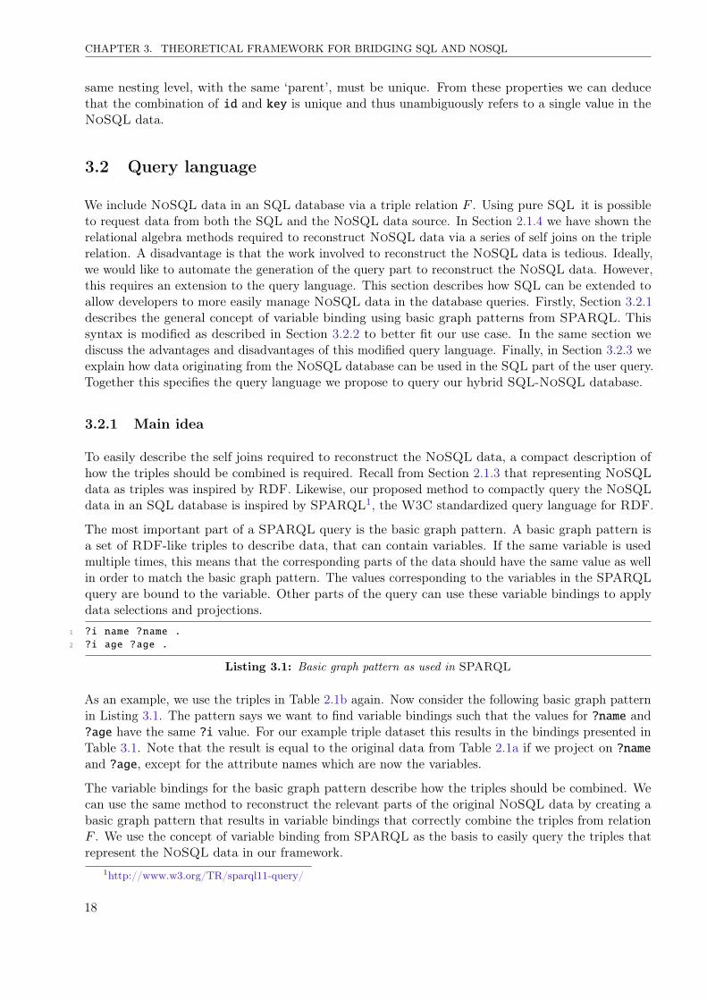
The most important part of a SPARQL query is the basic graph pattern. A basic graph pattern isa set of RDF-like triples to describe data, that can contain variables. If the same variable is usedmultiple times, this means that the corresponding parts of the data should have the same value as wellin order to match the basic graph pattern. The values corresponding to the variables in the SPARQLquery are bound to the variable. Other parts of the query can use these variable bindings to applydata selections and projections.
1 ?i name ?name .2 ?i age ?age .
Listing 3.1: Basic graph pattern as used in SPARQL
As an example, we use the triples in Table 2.1b again. Now consider the following basic graph patternin Listing 3.1. The pattern says we want to find variable bindings such that the values for ?name and?age have the same ?i value. For our example triple dataset this results in the bindings presented inTable 3.1. Note that the result is equal to the original data from Table 2.1a if we project on ?nameand ?age, except for the attribute names which are now the variables.
The variable bindings for the basic graph pattern describe how the triples should be combined. Wecan use the same method to reconstruct the relevant parts of the original NoSQL data by creating abasic graph pattern that results in variable bindings that correctly combine the triples from relationF . We use the concept of variable binding from SPARQL as the basis to easily query the triples thatrepresent the NoSQL data in our framework.
1http://www.w3.org/TR/sparql11-query/
18
3.2. QUERY LANGUAGE
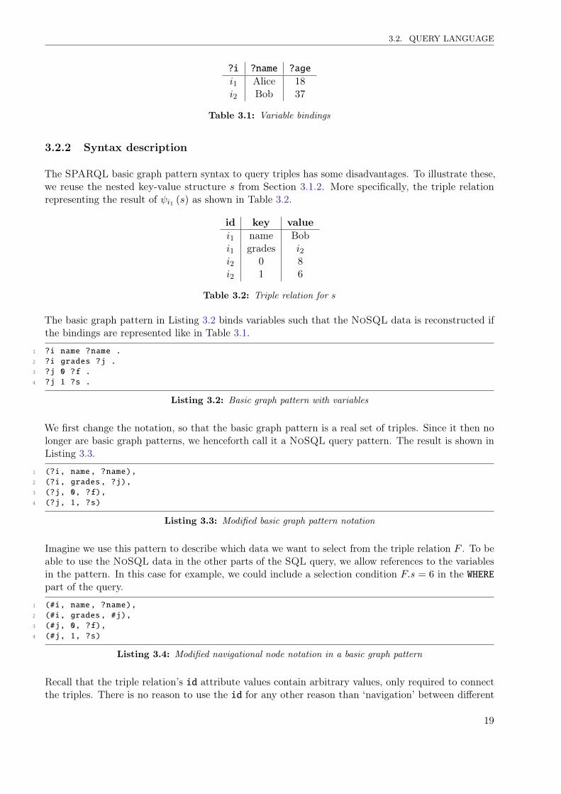
?i ?name ?age
i1 Alice 18i2 Bob 37
Table 3.1: Variable bindings
3.2.2 Syntax description
The SPARQL basic graph pattern syntax to query triples has some disadvantages. To illustrate these,we reuse the nested key-value structure s from Section 3.1.2. More specifically, the triple relationrepresenting the result of ψi1 (s) as shown in Table 3.2.
id key valuei1 name Bobi1 grades i2i2 0 8i2 1 6
Table 3.2: Triple relation for s
The basic graph pattern in Listing 3.2 binds variables such that the NoSQL data is reconstructed ifthe bindings are represented like in Table 3.1.
1 ?i name ?name .2 ?i grades ?j .3 ?j 0 ?f .4 ?j 1 ?s .
Listing 3.2: Basic graph pattern with variables
We first change the notation, so that the basic graph pattern is a real set of triples. Since it then nolonger are basic graph patterns, we henceforth call it a NoSQL query pattern. The result is shown inListing 3.3.
1 (?i, name, ?name),2 (?i, grades, ?j),3 (?j, 0, ?f),4 (?j, 1, ?s)
Listing 3.3: Modified basic graph pattern notation
Imagine we use this pattern to describe which data we want to select from the triple relation F . To beable to use the NoSQL data in the other parts of the SQL query, we allow references to the variablesin the pattern. In this case for example, we could include a selection condition F.s = 6 in the WHEREpart of the query.
1 (#i, name, ?name),2 (#i, grades, #j),3 (#j, 0, ?f),4 (#j, 1, ?s)
Listing 3.4: Modified navigational node notation in a basic graph pattern
Recall that the triple relation’s id attribute values contain arbitrary values, only required to connectthe triples. There is no reason to use the id for any other reason than ‘navigation’ between different
19
CHAPTER 3. THEORETICAL FRAMEWORK FOR BRIDGING SQL AND NOSQL
triples. Therefore, we adjust the notation for this type of variable. Instead of ?v, we denote themas #v. Furthermore, we disallow these navigational variables to be used outside the NoSQL querypattern. Listing 3.4 displays this adjustment.
Note that each triple in the NoSQL query pattern contains at least one navigational variable.Especially if a data object has many attributes, the NoSQL query pattern may contain just as manytriples with the same navigational variable to connect them. To avoid this, we combine differentNoSQL query pattern triples into a nested key-value set if they have the same navigational variableas their id value. Also, we can nest these key-value pairs, when appropriate, in order to further reducethe overhead in the NoSQL query pattern. For our example, this means that the triples with keyvalues name and grades can be combined, and that #j can be nested under the (#i, grades, #j)triple as illustrated in Listing 3.5.
1 (2 name: ?name,3 grades: (4 0: ?f,5 1: ?s6 )7 )
Listing 3.5: NoSQL query pattern
In our example NoSQL query pattern there was only one triple with #j as its value under whichwe could nest the triples with id value #j. In general however, it is possible that there are multipletriples with the same variable as value to nest the data, as exemplified in Listing 3.6.
1 (#i, from, #j),2 (#i, to, #j),3 (#j, name, ?name)
Listing 3.6: Basic graph pattern that cannot be represented as a NoSQL query pattern
In this case the (#j, name, ?name) triple can be nested under both other triples, which results inthe other triple still having the #j as its value. There is no way to indicate that from and to shouldhave equal values using this syntax. Furthermore, we only allow one pattern to be used as a query.This means that we can only specify conditions for one NoSQL data entity, and it also implies thatour previous example where nesting can be done in multiple ways is not supported by a NoSQL querypattern. For the empirical analysis of our prototype we take this into account and ensure this notationsupports all our test queries. In general however, this is a significant limitation to the expressivenessof the query language and certainly an important point for future improvement.
Note that the NoSQL query pattern notation is almost similar to the nested key-value structurenotation we introduced in Section 3.1.2. Instead of a set notation we use normal parentheses, andwe allow keys and values to be replaced by variables. Recall from the same section that we usedthe nested key-value structure to transform NoSQL data to a triple representation. For our querylanguage we now do the reverse, and use the nested key-value notation to describe which triples wewant to query and how they are related.
As also described in the previously referred section, keys in the nested key-value structure to describethe NoSQL on the same nesting level, with the same ‘parent’, must be unique. Likewise, we requirethat keys in the same nested key-value set of a NoSQL query pattern are unique. Though this limitsthe expressiveness of the query language, it is a minor restrictions. The NoSQL data cannot containmultiple triples for a combination of id and key, so in practice there is no need to construct such aNoSQL query pattern.
20
3.3. ARCHITECTURAL OVERVIEW
3.2.3 Collaboration with SQL
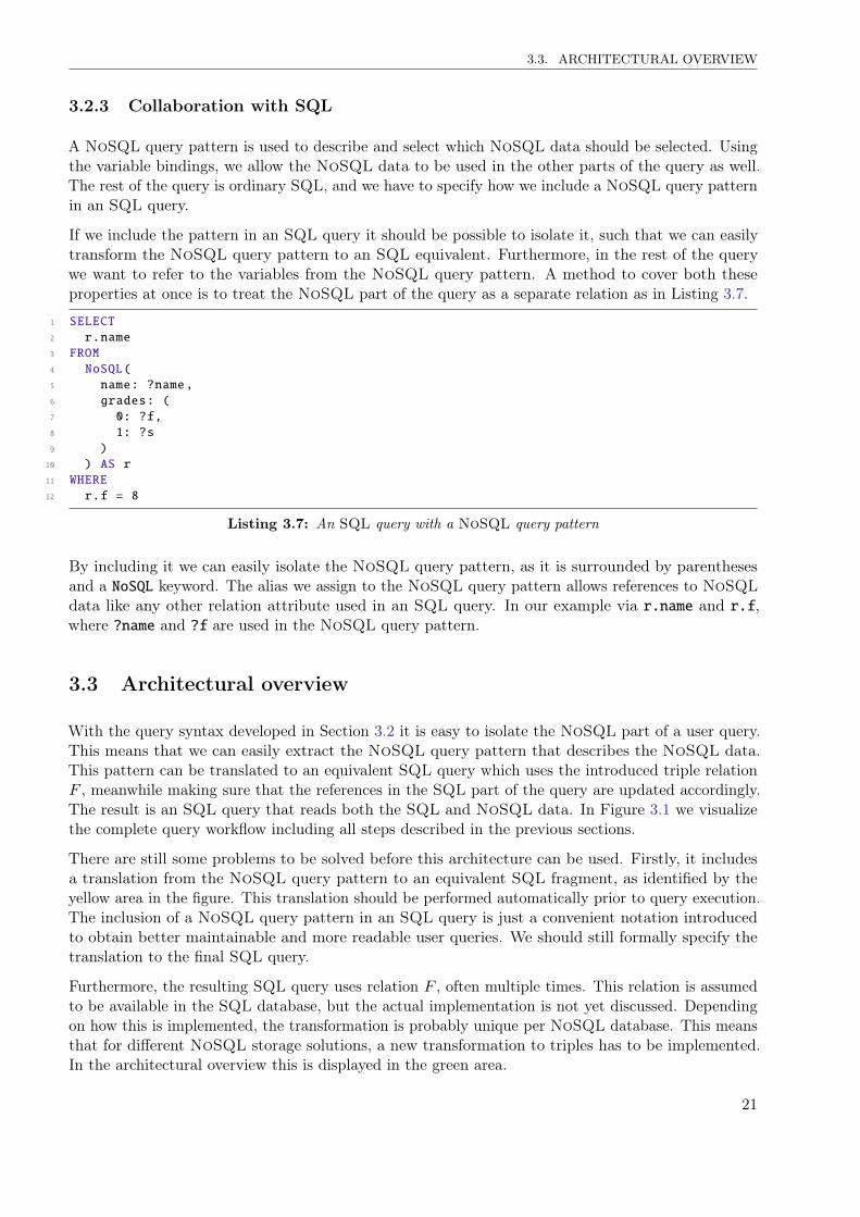
A NoSQL query pattern is used to describe and select which NoSQL data should be selected. Usingthe variable bindings, we allow the NoSQL data to be used in the other parts of the query as well.The rest of the query is ordinary SQL, and we have to specify how we include a NoSQL query patternin an SQL query.
If we include the pattern in an SQL query it should be possible to isolate it, such that we can easilytransform the NoSQL query pattern to an SQL equivalent. Furthermore, in the rest of the querywe want to refer to the variables from the NoSQL query pattern. A method to cover both theseproperties at once is to treat the NoSQL part of the query as a separate relation as in Listing 3.7.
1 SELECT2 r.name3 FROM4 NoSQL(5 name: ?name,6 grades: (7 0: ?f,8 1: ?s9 )10 ) AS r11 WHERE12 r.f = 8
Listing 3.7: An SQL query with a NoSQL query pattern
By including it we can easily isolate the NoSQL query pattern, as it is surrounded by parenthesesand a NoSQL keyword. The alias we assign to the NoSQL query pattern allows references to NoSQLdata like any other relation attribute used in an SQL query. In our example via r.name and r.f,where ?name and ?f are used in the NoSQL query pattern.
3.3 Architectural overview
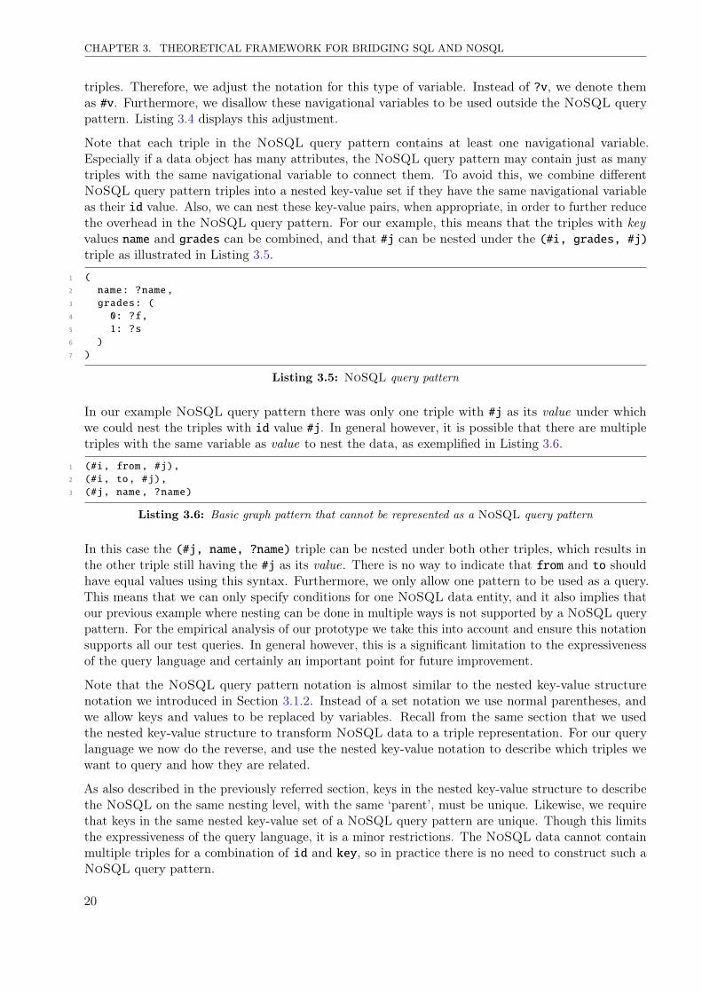
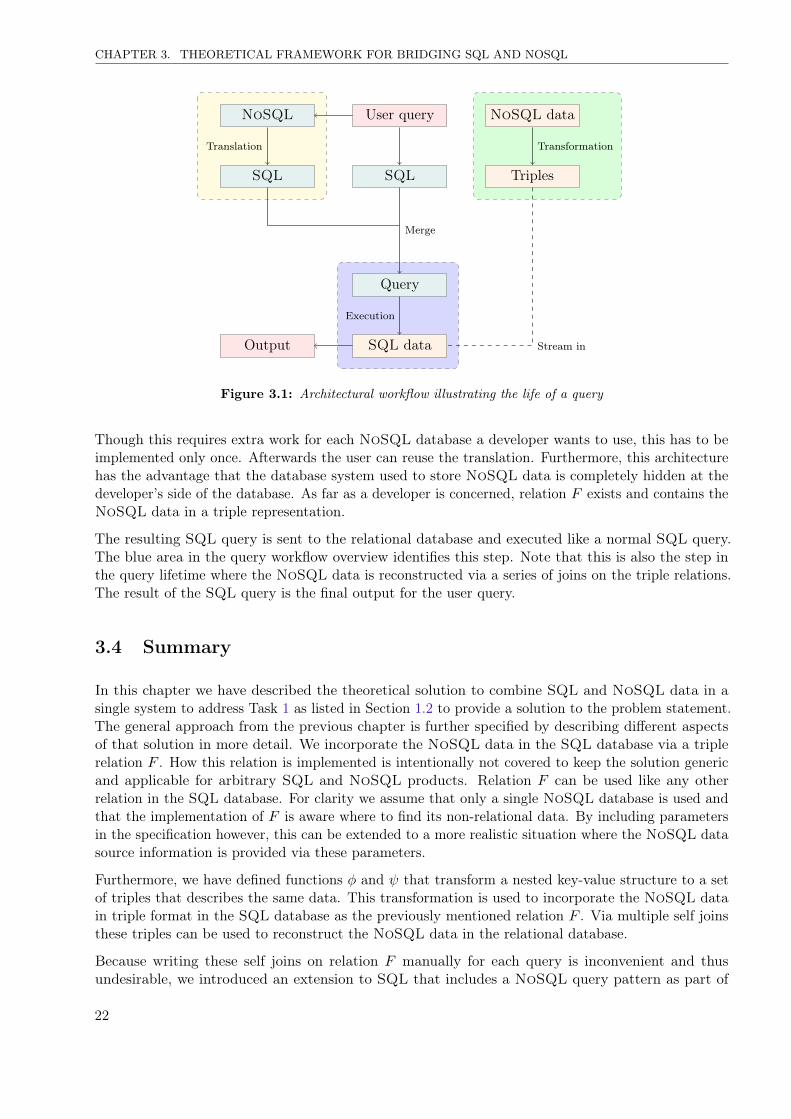
With the query syntax developed in Section 3.2 it is easy to isolate the NoSQL part of a user query.This means that we can easily extract the NoSQL query pattern that describes the NoSQL data.This pattern can be translated to an equivalent SQL query which uses the introduced triple relationF , meanwhile making sure that the references in the SQL part of the query are updated accordingly.The result is an SQL query that reads both the SQL and NoSQL data. In Figure 3.1 we visualizethe complete query workflow including all steps described in the previous sections.
There are still some problems to be solved before this architecture can be used. Firstly, it includesa translation from the NoSQL query pattern to an equivalent SQL fragment, as identified by theyellow area in the figure. This translation should be performed automatically prior to query execution.The inclusion of a NoSQL query pattern in an SQL query is just a convenient notation introducedto obtain better maintainable and more readable user queries. We should still formally specify thetranslation to the final SQL query.
Furthermore, the resulting SQL query uses relation F , often multiple times. This relation is assumedto be available in the SQL database, but the actual implementation is not yet discussed. Dependingon how this is implemented, the transformation is probably unique per NoSQL database. This meansthat for different NoSQL storage solutions, a new transformation to triples has to be implemented.In the architectural overview this is displayed in the green area.
21
CHAPTER 3. THEORETICAL FRAMEWORK FOR BRIDGING SQL AND NOSQL
User query
SQL
NoSQL
SQL
Translation
Query
Merge
NoSQL data
Triples
Transformation
SQL data
Execution
Stream inOutput
Figure 3.1: Architectural workflow illustrating the life of a query
Though this requires extra work for each NoSQL database a developer wants to use, this has to beimplemented only once. Afterwards the user can reuse the translation. Furthermore, this architecturehas the advantage that the database system used to store NoSQL data is completely hidden at thedeveloper’s side of the database. As far as a developer is concerned, relation F exists and contains theNoSQL data in a triple representation.
The resulting SQL query is sent to the relational database and executed like a normal SQL query.The blue area in the query workflow overview identifies this step. Note that this is also the step inthe query lifetime where the NoSQL data is reconstructed via a series of joins on the triple relations.The result of the SQL query is the final output for the user query.
3.4 Summary
In this chapter we have described the theoretical solution to combine SQL and NoSQL data in asingle system to address Task 1 as listed in Section 1.2 to provide a solution to the problem statement.The general approach from the previous chapter is further specified by describing different aspectsof that solution in more detail. We incorporate the NoSQL data in the SQL database via a triplerelation F . How this relation is implemented is intentionally not covered to keep the solution genericand applicable for arbitrary SQL and NoSQL products. Relation F can be used like any otherrelation in the SQL database. For clarity we assume that only a single NoSQL database is used andthat the implementation of F is aware where to find its non-relational data. By including parametersin the specification however, this can be extended to a more realistic situation where the NoSQL datasource information is provided via these parameters.
Furthermore, we have defined functions φ and ψ that transform a nested key-value structure to a setof triples that describes the same data. This transformation is used to incorporate the NoSQL datain triple format in the SQL database as the previously mentioned relation F . Via multiple self joinsthese triples can be used to reconstruct the NoSQL data in the relational database.
Because writing these self joins on relation F manually for each query is inconvenient and thusundesirable, we introduced an extension to SQL that includes a NoSQL query pattern as part of
22

3.4. SUMMARY
the query. Inspired by SPARQL, a NoSQL query pattern describes which data from relation F wewant to use. Using variable bindings, the corresponding NoSQL data can be used in the rest of theSQL query as if it are attributes of a normal relation. The result is a user query containing a NoSQLquery pattern in an ordinary SQL query, that is translated to an equivalent pure SQL query in whichmultiple copies of relation F are used and the self join conditions are automatically added. Lastly, weprovided an architectural overview following the query workflow. This gives a global overview of thesteps involved from the moment a developer sends a query until the query result is generated. Thefollowing chapter is dedicated to explaining how the translation from a user query with a NoSQLquery pattern to a pure SQL equivalent can be performed automatically.
23

4Query processing strategies
To avoid that the developer should manually reconstruct the NoSQL data from the triple relation F ,we have introduced a NoSQL query pattern in the previous chapter. This pattern can be included inan SQL query to describe which NoSQL data should be selected. These patterns are convenient forthe developer, but the language extension requires us to first translate the user query before we havea valid SQL query that can be executed. In Section 4.1 we describe the minimum translation requiredto obtain an SQL query that produces the correct result, and also describe how selections can bepushed down such that the translation can be improved and the correct result is obtained within amore acceptable time. As described in Task 2 the translations are formally specified to provide agenerically applicable solution. We therefore give the translation in relational algebra notation.
The other sections in this chapter describe further improvements which we apply to decrease theaverage query execution time and to obtain a feasible prototype. Firstly, Section 4.2 explains howprojections can be pushed down the same way as we push selections down. This reduces the amount oftriples each copy of F in the resulting SQL query contains. Because each copy of F retrieves the sameset of triples, we describe a method to retrieve these triples only once and then reuse them at the SQLside of the implementation in Section 4.3. An overview of all steps in the entire translation is given inSection 4.4. Together these steps automatically translate and optimize the NoSQL query pattern inthe user query to the series of self joins that lead to the correct reconstruction of the NoSQL data inthe relational database.
4.1 Base implementation
This section describes the base translation from the user query with a NoSQL query pattern to a pureSQL equivalent. Before we dive into the translation itself, we first describe some notation conventionsin Section 4.1.1. The base translation specified in Section 4.1.2 is the minimal work required to obtainan SQL query that results in the correct output. This translation only focuses on the yellow area inthe query workflow overview, and thus does not restrict the set of triples shipped from the NoSQLto the SQL database. Therefore, this is quite a naive translation and far from efficient enough tobe feasible in practical situations. Therefore, we provide additional query processing strategies tooptimize the translation, like the selection pushdown discussed in Section 4.1.3. As a result of theselection pushdown, the amount of triples to represent the NoSQL data is reduced. Therefore, thisselection pushdown strategy aims at optimizing the work in the green area of the query workflow. Thisselection pushdown can be improved by combining selection conditions as explained in Section 4.1.4.
25
CHAPTER 4. QUERY PROCESSING STRATEGIES
A final addition to the base translation is the constraint derivation described in Section 4.1.5. Like forthe selection pushdown, this optimization can also be improved by applying transitivity following therules provided in Section 4.1.6.
4.1.1 Notation
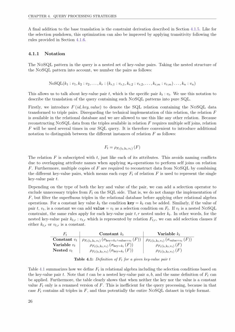
The NoSQL pattern in the query is a nested set of key-value pairs. Taking the nested structure ofthe NoSQL pattern into account, we number the pairs as follows:
NoSQL(k1 : v1, k2 : v2, . . . , kr : (kr,1 : vr,1, kr,2 : vr,2, . . . , kr,m : vr,m) . . . , kn : vn)
This allows us to talk about key-value pair t, which is the specific pair kt : vt. We use this notation todescribe the translation of the query containing such NoSQL patterns into pure SQL.
Firstly, we introduce F (id, key, value) to denote the SQL relation containing the NoSQL datatransformed to triple pairs. Disregarding the technical implementation of this relation, the relation Fis available in the relational database and we are allowed to use this like any other relation. Becausereconstructing NoSQL data from the triples available in relation F requires multiple self joins, relationF will be used several times in our SQL query. It is therefore convenient to introduce additionalnotation to distinguish between the different instances of relation F as follows:
Ft = ρFt(it,kt,vt) (F )
The relation F is subscripted with t, just like each of its attributes. This avoids naming conflictsdue to overlapping attribute names when applying onθ-operations to perform self joins on relationF . Furthermore, multiple copies of F are required to reconstruct data from NoSQL by combiningthe different key-value pairs, which means each copy Ft of relation F is used to represent the singlekey-value pair t.
Depending on the type of both the key and value of the pair, we can add a selection operator toexclude unnecessary triples from Ft on the SQL side. That is, we do not change the implementation ofF , but filter the superfluous triples in the relational database before applying other relational algebraoperations. For a constant key value kt the condition key = kt can be added. Similarly, if the value ofpair t, vt, is a constant we can add value = vt as a selection condition on Ft. If vt is a nested NoSQLconstraint, the same rules apply for each key-value pair t, r nested under kt. In other words, for thenested key-value pair kt,r : vt,r which is represented by relation Ft,r, we can add selection clauses ifeither kt,r or vt,r is a constant.
Ft Constant kt Variable ktConstant vt ρFt(it,kt,vt) (σkey=kt∧value=vt (F )) ρFt(it,kt,vt) (σvalue=vt (F ))
Variable vt ρFt(it,kt,vt) (σkey=kt (F )) ρFt(it,kt,vt) (F )
Nested vt ρFt(it,kt,vt) (σkey=kt (F )) ρFt(it,kt,vt) (F )
Table 4.1: Definition of Ft for a given key-value pair t
Table 4.1 summarizes how we define Ft in relational algebra including the selection conditions based onthe key-value pair t. Note that t can be a nested key-value pair a, b, and the same definition of Ft canbe applied. Furthermore, the table clearly shows that when neither the key nor the value is a constantvalue Ft only is a renamed version of F . This is inefficient for the query processing, because in thatcase Ft contains all triples in F , and thus potentially the entire NoSQL dataset in triple format.
26
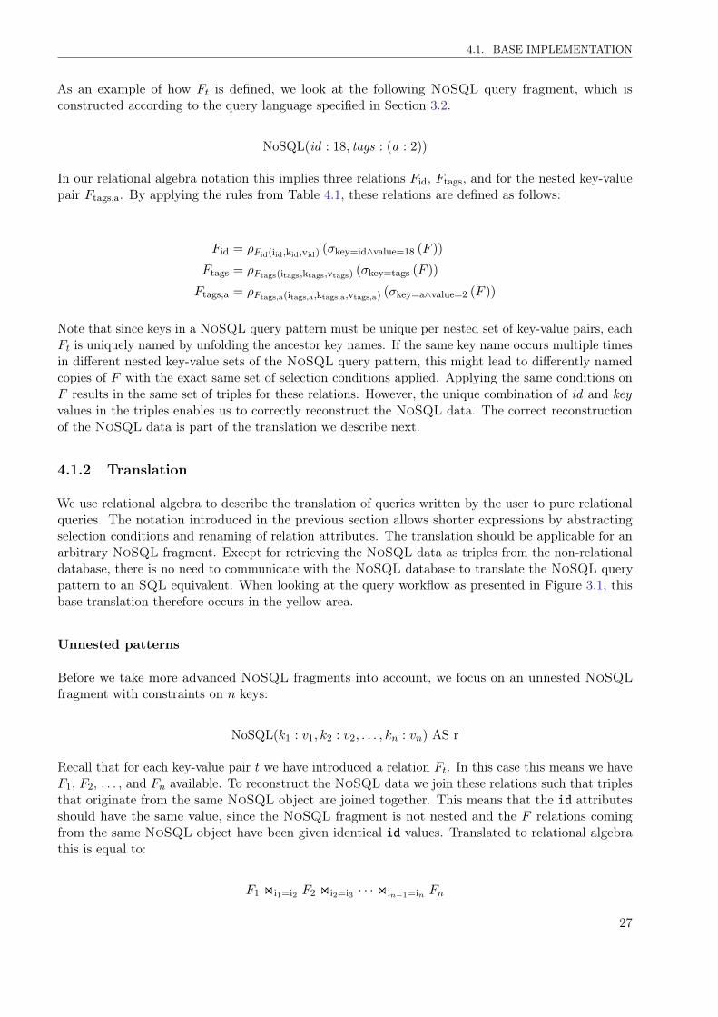
4.1. BASE IMPLEMENTATION
As an example of how Ft is defined, we look at the following NoSQL query fragment, which isconstructed according to the query language specified in Section 3.2.
NoSQL(id : 18, tags : (a : 2))
In our relational algebra notation this implies three relations Fid, Ftags, and for the nested key-valuepair Ftags,a. By applying the rules from Table 4.1, these relations are defined as follows:
Fid = ρFid(iid,kid,vid) (σkey=id∧value=18 (F ))
Ftags = ρFtags(itags,ktags,vtags) (σkey=tags (F ))
Ftags,a = ρFtags,a(itags,a,ktags,a,vtags,a) (σkey=a∧value=2 (F ))
Note that since keys in a NoSQL query pattern must be unique per nested set of key-value pairs, eachFt is uniquely named by unfolding the ancestor key names. If the same key name occurs multiple timesin different nested key-value sets of the NoSQL query pattern, this might lead to differently namedcopies of F with the exact same set of selection conditions applied. Applying the same conditions onF results in the same set of triples for these relations. However, the unique combination of id and keyvalues in the triples enables us to correctly reconstruct the NoSQL data. The correct reconstructionof the NoSQL data is part of the translation we describe next.
4.1.2 Translation
We use relational algebra to describe the translation of queries written by the user to pure relationalqueries. The notation introduced in the previous section allows shorter expressions by abstractingselection conditions and renaming of relation attributes. The translation should be applicable for anarbitrary NoSQL fragment. Except for retrieving the NoSQL data as triples from the non-relationaldatabase, there is no need to communicate with the NoSQL database to translate the NoSQL querypattern to an SQL equivalent. When looking at the query workflow as presented in Figure 3.1, thisbase translation therefore occurs in the yellow area.
Unnested patterns
Before we take more advanced NoSQL fragments into account, we focus on an unnested NoSQLfragment with constraints on n keys:
NoSQL(k1 : v1, k2 : v2, . . . , kn : vn) AS r
Recall that for each key-value pair t we have introduced a relation Ft. In this case this means we haveF1, F2, . . . , and Fn available. To reconstruct the NoSQL data we join these relations such that triplesthat originate from the same NoSQL object are joined together. This means that the id attributesshould have the same value, since the NoSQL fragment is not nested and the F relations comingfrom the same NoSQL object have been given identical id values. Translated to relational algebrathis is equal to:
F1 oni1=i2 F2 oni2=i3 · · · onin−1=in Fn
27
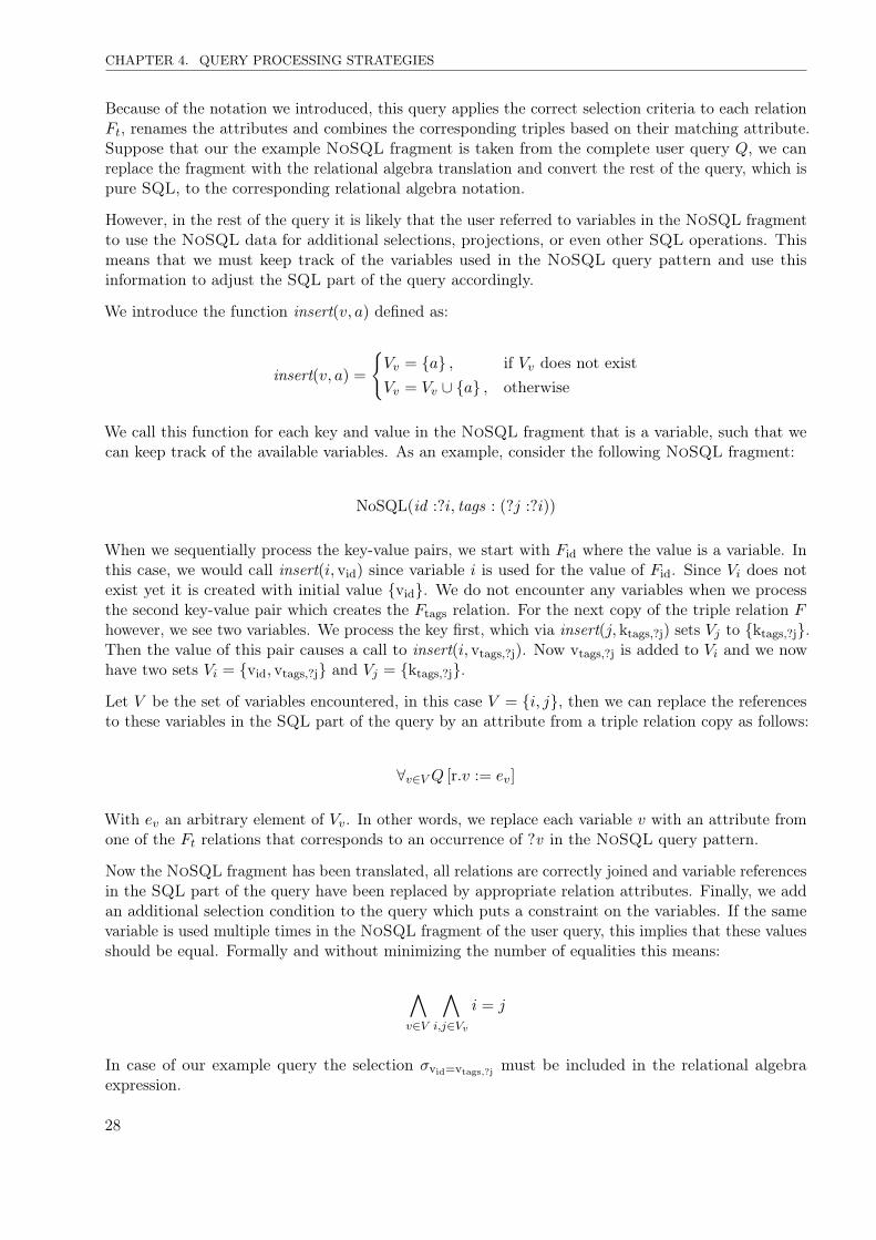
CHAPTER 4. QUERY PROCESSING STRATEGIES
Because of the notation we introduced, this query applies the correct selection criteria to each relationFt, renames the attributes and combines the corresponding triples based on their matching attribute.Suppose that our the example NoSQL fragment is taken from the complete user query Q, we canreplace the fragment with the relational algebra translation and convert the rest of the query, which ispure SQL, to the corresponding relational algebra notation.
However, in the rest of the query it is likely that the user referred to variables in the NoSQL fragmentto use the NoSQL data for additional selections, projections, or even other SQL operations. Thismeans that we must keep track of the variables used in the NoSQL query pattern and use thisinformation to adjust the SQL part of the query accordingly.
We introduce the function insert(v, a) defined as:
insert(v, a) =
{Vv = {a} , if Vv does not existVv = Vv ∪ {a} , otherwise
We call this function for each key and value in the NoSQL fragment that is a variable, such that wecan keep track of the available variables. As an example, consider the following NoSQL fragment:
NoSQL(id :?i, tags : (?j :?i))
When we sequentially process the key-value pairs, we start with Fid where the value is a variable. Inthis case, we would call insert(i, vid) since variable i is used for the value of Fid. Since Vi does notexist yet it is created with initial value {vid}. We do not encounter any variables when we processthe second key-value pair which creates the Ftags relation. For the next copy of the triple relation Fhowever, we see two variables. We process the key first, which via insert(j, ktags,?j) sets Vj to {ktags,?j}.Then the value of this pair causes a call to insert(i, vtags,?j). Now vtags,?j is added to Vi and we nowhave two sets Vi = {vid, vtags,?j} and Vj = {ktags,?j}.
Let V be the set of variables encountered, in this case V = {i, j}, then we can replace the referencesto these variables in the SQL part of the query by an attribute from a triple relation copy as follows:
∀v∈VQ [r.v := ev]
With ev an arbitrary element of Vv. In other words, we replace each variable v with an attribute fromone of the Ft relations that corresponds to an occurrence of ?v in the NoSQL query pattern.
Now the NoSQL fragment has been translated, all relations are correctly joined and variable referencesin the SQL part of the query have been replaced by appropriate relation attributes. Finally, we addan additional selection condition to the query which puts a constraint on the variables. If the samevariable is used multiple times in the NoSQL fragment of the user query, this implies that these valuesshould be equal. Formally and without minimizing the number of equalities this means:
∧v∈V
∧i,j∈Vv
i = j
In case of our example query the selection σvid=vtags,?j must be included in the relational algebraexpression.
28
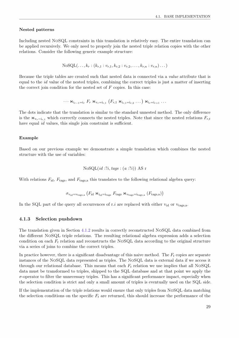
4.1. BASE IMPLEMENTATION
Nested patterns
Including nested NoSQL constraints in this translation is relatively easy. The entire translation canbe applied recursively. We only need to properly join the nested triple relation copies with the otherrelations. Consider the following generic example structure:
NoSQL(. . . , kr : (kr,1 : vr,1, kr,2 : vr,2, . . . , kr,n : vr,n) . . . )
Because the triple tables are created such that nested data is connected via a value attribute that isequal to the id value of the nested triples, combining the correct triples is just a matter of insertingthe correct join condition for the nested set of F copies. In this case:
· · · onir−1=ir Fr onvr=ir,1(Fr,1 onir,1=ir,2 . . .
)onir=ir+1 . . .
The dots indicate that the translation is similar to the standard unnested method. The only differenceis the onvr=ir,1 which correctly connects the nested triples. Note that since the nested relations Fr,thave equal id values, this single join constraint is sufficient.
Example
Based on our previous example we demonstrate a simple translation which combines the nestedstructure with the use of variables:
NoSQL(id :?i, tags : (a :?i)) AS r
With relations Fid, Ftags, and Ftags,a this translates to the following relational algebra query:
σvid=vtags,a
(Fid oniid=itags Ftags onvtags=itags,a (Ftags,a)
)In the SQL part of the query all occurrences of r.i are replaced with either vid or vtags,a.
4.1.3 Selection pushdown
The translation given in Section 4.1.2 results in correctly reconstructed NoSQL data combined fromthe different NoSQL triple relations. The resulting relational algebra expression adds a selectioncondition on each Ft relation and reconstructs the NoSQL data according to the original structurevia a series of joins to combine the correct triples.
In practice however, there is a significant disadvantage of this naive method. The Ft copies are separateinstances of the NoSQL data represented as triples. The NoSQL data is external data if we access itthrough our relational database. This means that each Ft relation we use implies that all NoSQLdata must be transformed to triples, shipped to the SQL database and at that point we apply theσ-operator to filter the unnecessary triples. This has a significant performance impact, especially whenthe selection condition is strict and only a small amount of triples is eventually used on the SQL side.
If the implementation of the triple relations would ensure that only triples from NoSQL data matchingthe selection conditions on the specific Ft are returned, this should increase the performance of the
29
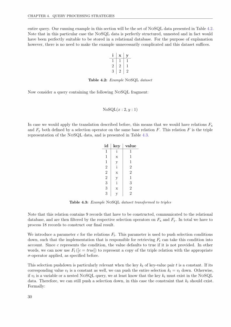
CHAPTER 4. QUERY PROCESSING STRATEGIES
entire query. Our running example in this section will be the set of NoSQL data presented in Table 4.2.Note that in this particular case the NoSQL data is perfectly structured, unnested and in fact wouldhave been perfectly suitable to be stored in a relational database. For the purpose of explanationhowever, there is no need to make the example unnecessarily complicated and this dataset suffices.
i x y1 1 12 2 13 2 2
Table 4.2: Example NoSQL dataset
Now consider a query containing the following NoSQL fragment:
NoSQL(x : 2, y : 1)
In case we would apply the translation described before, this means that we would have relations Fxand Fy both defined by a selection operator on the same base relation F . This relation F is the triplerepresentation of the NoSQL data, and is presented in Table 4.3.
id key value1 i 11 x 11 y 12 i 22 x 22 y 13 i 33 x 23 y 2
Table 4.3: Example NoSQL dataset transformed to triples
Note that this relation contains 9 records that have to be constructed, communicated to the relationaldatabase, and are then filtered by the respective selection operators on Fx and Fy. In total we have toprocess 18 records to construct our final result.
We introduce a parameter c for the relations Ft. This parameter is used to push selection conditionsdown, such that the implementation that is responsible for retrieving Ft can take this condition intoaccount. Since c represents the condition, the value defaults to true if it is not provided. In otherwords, we can now use Ft ([c = true]) to represent a copy of the triple relation with the appropriateσ-operator applied, as specified before.
This selection pushdown is particularly relevant when the key kt of key-value pair t is a constant. If itscorresponding value vt is a constant as well, we can push the entire selection kt = vt down. Otherwise,if vt is a variable or a nested NoSQL query, we at least know that the key kt must exist in the NoSQLdata. Therefore, we can still push a selection down, in this case the constraint that kt should exist.Formally:
30
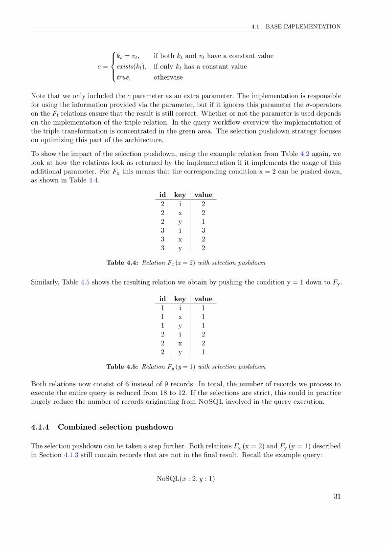
4.1. BASE IMPLEMENTATION
c =
kt = vt, if both kt and vt have a constant valueexists(kt), if only kt has a constant valuetrue, otherwise
Note that we only included the c parameter as an extra parameter. The implementation is responsiblefor using the information provided via the parameter, but if it ignores this parameter the σ-operatorson the Ft relations ensure that the result is still correct. Whether or not the parameter is used dependson the implementation of the triple relation. In the query workflow overview the implementation ofthe triple transformation is concentrated in the green area. The selection pushdown strategy focuseson optimizing this part of the architecture.
To show the impact of the selection pushdown, using the example relation from Table 4.2 again, welook at how the relations look as returned by the implementation if it implements the usage of thisadditional parameter. For Fx this means that the corresponding condition x = 2 can be pushed down,as shown in Table 4.4.
id key value2 i 22 x 22 y 13 i 33 x 23 y 2
Table 4.4: Relation Fx (x = 2) with selection pushdown
Similarly, Table 4.5 shows the resulting relation we obtain by pushing the condition y = 1 down to Fy.
id key value1 i 11 x 11 y 12 i 22 x 22 y 1
Table 4.5: Relation Fy (y = 1) with selection pushdown
Both relations now consist of 6 instead of 9 records. In total, the number of records we process toexecute the entire query is reduced from 18 to 12. If the selections are strict, this could in practicehugely reduce the number of records originating from NoSQL involved in the query execution.
4.1.4 Combined selection pushdown
The selection pushdown can be taken a step further. Both relations Fx (x = 2) and Fy (y = 1) describedin Section 4.1.3 still contain records that are not in the final result. Recall the example query:
NoSQL(x : 2, y : 1)
31
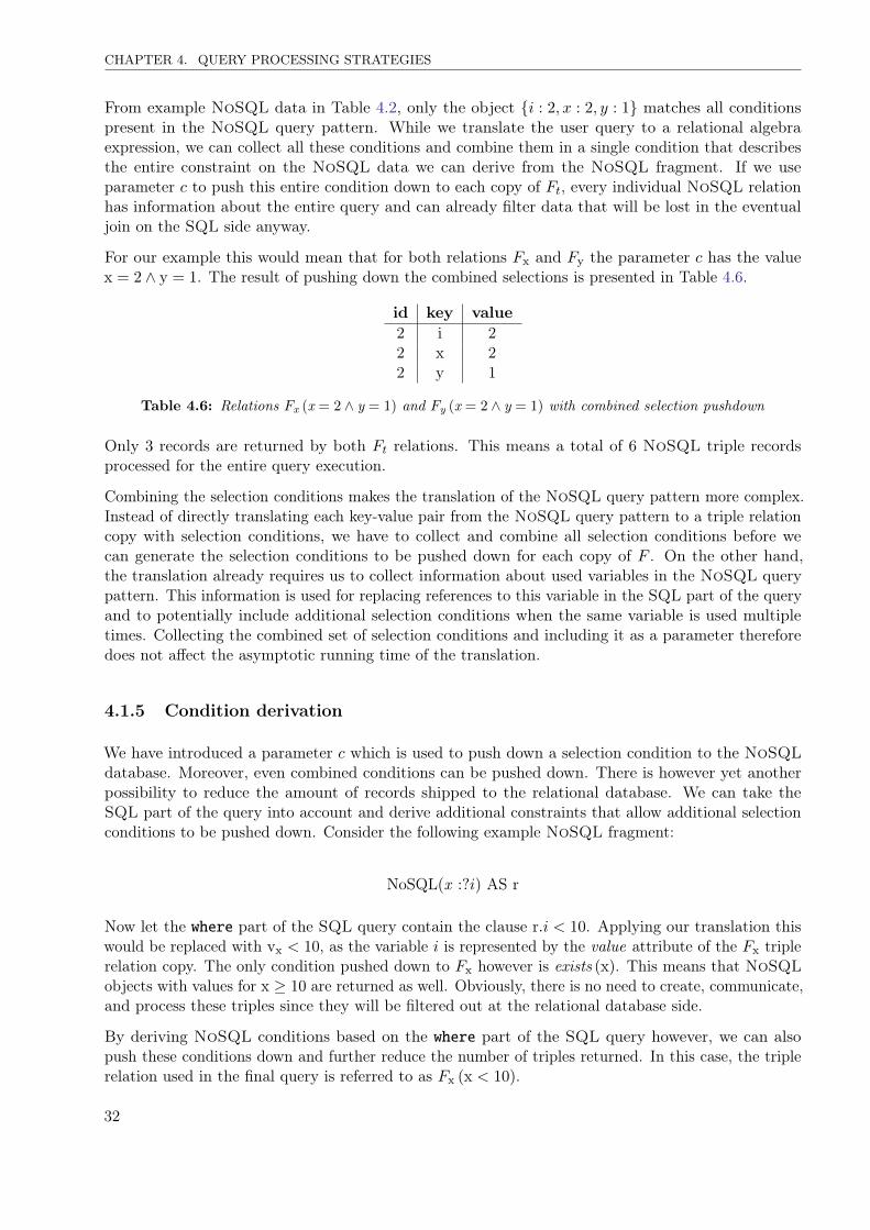
CHAPTER 4. QUERY PROCESSING STRATEGIES
From example NoSQL data in Table 4.2, only the object {i : 2, x : 2, y : 1} matches all conditionspresent in the NoSQL query pattern. While we translate the user query to a relational algebraexpression, we can collect all these conditions and combine them in a single condition that describesthe entire constraint on the NoSQL data we can derive from the NoSQL fragment. If we useparameter c to push this entire condition down to each copy of Ft, every individual NoSQL relationhas information about the entire query and can already filter data that will be lost in the eventualjoin on the SQL side anyway.
For our example this would mean that for both relations Fx and Fy the parameter c has the valuex = 2 ∧ y = 1. The result of pushing down the combined selections is presented in Table 4.6.
id key value2 i 22 x 22 y 1
Table 4.6: Relations Fx (x = 2 ∧ y = 1) and Fy (x = 2 ∧ y = 1) with combined selection pushdown
Only 3 records are returned by both Ft relations. This means a total of 6 NoSQL triple recordsprocessed for the entire query execution.
Combining the selection conditions makes the translation of the NoSQL query pattern more complex.Instead of directly translating each key-value pair from the NoSQL query pattern to a triple relationcopy with selection conditions, we have to collect and combine all selection conditions before wecan generate the selection conditions to be pushed down for each copy of F . On the other hand,the translation already requires us to collect information about used variables in the NoSQL querypattern. This information is used for replacing references to this variable in the SQL part of the queryand to potentially include additional selection conditions when the same variable is used multipletimes. Collecting the combined set of selection conditions and including it as a parameter thereforedoes not affect the asymptotic running time of the translation.
4.1.5 Condition derivation
We have introduced a parameter c which is used to push down a selection condition to the NoSQLdatabase. Moreover, even combined conditions can be pushed down. There is however yet anotherpossibility to reduce the amount of records shipped to the relational database. We can take theSQL part of the query into account and derive additional constraints that allow additional selectionconditions to be pushed down. Consider the following example NoSQL fragment:
NoSQL(x :?i) AS r
Now let the where part of the SQL query contain the clause r.i < 10. Applying our translation thiswould be replaced with vx < 10, as the variable i is represented by the value attribute of the Fx triplerelation copy. The only condition pushed down to Fx however is exists (x). This means that NoSQLobjects with values for x ≥ 10 are returned as well. Obviously, there is no need to create, communicate,and process these triples since they will be filtered out at the relational database side.
By deriving NoSQL conditions based on the where part of the SQL query however, we can alsopush these conditions down and further reduce the number of triples returned. In this case, the triplerelation used in the final query is referred to as Fx (x < 10).
32
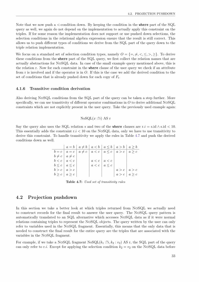
4.2. PROJECTION PUSHDOWN
Note that we now push a <-condition down. By keeping the condition in the where part of the SQLquery as well, we again do not depend on the implementation to actually apply this constraint on thetriples. If for some reason the implementation does not support or use pushed down selections, theselection conditions in the relational algebra expression ensure that the result is still correct. Thisallows us to push different types of conditions we derive from the SQL part of the query down to thetriple relation implementation.
We focus on a standard set of selection condition types, namely O = {=, 6=, <,≤, >,≥}. To derivethese conditions from the where part of the SQL query, we first collect the relation names that areactually abstractions for NoSQL data. In case of the small example query mentioned above, this isthe relation r. Now for each constraint in the where clause of the user query we check if an attributefrom r is involved and if the operator is in O. If this is the case we add the derived condition to theset of conditions that is already pushed down for each copy of Ft.
4.1.6 Transitive condition derivation
Also deriving NoSQL conditions from the SQL part of the query can be taken a step further. Morespecifically, we can use transitivity of different operator combinations in O to derive additional NoSQLconstraints which are not explicitly present in the user query. Take the previously used example again:
NoSQL(x :?i) AS r
Say the query also uses the SQL relation s and two of the where clauses are r.i = s.id ∧ s.id < 10.This essentially adds the constraint r.i < 10 on the NoSQL data, only we have to use transitivity toderive this constraint. To handle transitivity we apply the rules in Table 4.7 and push the derivedconditions down as well.
a = b a 6= b a < b a ≤ b a > b a ≥ bb = c a = c a 6= c a < c a ≤ c a > c a ≥ cb 6= c a 6= cb < c a < c a < c a < cb ≤ c a ≤ c a < c a ≤ cb > c a > c a > c a > cb ≥ c a ≥ c a > c a ≥ c
Table 4.7: Used set of transitivity rules
4.2 Projection pushdown
In this section we take a better look at which triples returned from NoSQL we actually needto construct records for the final result to answer the user query. The NoSQL query pattern isautomatically translated to an SQL alternative which accesses NoSQL data as if it were normalrelations containing triples to represent the NoSQL objects. The query written by the user can onlyrefer to variables used in the NoSQL fragment. Essentially, this means that the only data that isneeded to construct the final result for the entire query are the triples that are associated with thevariables in the NoSQL fragment.
For example, if we take a NoSQL fragment NoSQL(k1 :?i, k2 : v2) AS r, the SQL part of the querycan only refer to r.i. Except for applying the selection condition k2 = v2 on the NoSQL data before
33
CHAPTER 4. QUERY PROCESSING STRATEGIES
returning anything, there is no need to ship triples containing any other data than k1 values forNoSQL objects which match the constraint k2 = v2. Moreover, if no variable from a NoSQL fragmentis referred to in the SQL part of the query, there is no need to access the NoSQL data source at all.
This observation leads to the concept we call projection pushdown. The set of key-value pairs forwhich a triple relation Ft is required to be able to access all needed information from the NoSQLquery pattern in the SQL part of the query is called If . In other words, for each NoSQL fragment fwe search for all occurrences of f.v for some variable v in the SQL part of the user query. For eachfound f.v we collect all Ft corresponding to key-value pairs from NoSQL fragment f for which eitherkt =?v or vt =?v and call this set If .
For example, consider the following NoSQL fragment f:
NoSQL(k1 :?i, k2 : (k2,1 : v2,1, k2,2 :?j, k2,3 : v2,3), k3 : v3) AS f
If the user query refers to f.i and f.j, this means If = {F1, F2,2} since the key-value pairs 1 and 2, 2contain variables which are referenced. To determine if for a given key-value pair t we should includeFt in the translation, we recursively determine if Ft is in If or, in case vt is nested, if there exists anested key-value pair under t which should be in the translation.
For our example this means we would have F1, F2, and F2,2 in the translation. Note that F2 is presentbecause F2,2 should be in the translation and F2 therefore is required to ensure the structure of theNoSQL data is maintained. Compared to the base translation, we do not use the relations F2,1, F2,3,and F3.
By reducing the number of relations that return triples we do not only decrease the amount of datathat has to be shipped from NoSQL to the relational database. The final query will also contain lessrelations and thus require less joins to reconstruct the NoSQL data in the relational database.
Besides reducing the number of triple relation copies Ft, we can use the information about whichvariables are used to reduce the amount of triples within a single triple relation copy as well. Considerthe previous example again. There is no need to include the triples representing the key-value pairsfor k3 : v3, since we do not use this information in the SQL query.
The unnecessary triples are excluded on the SQL side by the selection and join operators. In fact,the NoSQL data reconstruction filters the triples and thereby the NoSQL key-value pairs. This isessentially the same as a projection on a subset of attributes. Just like for selections, we can push thisprojection down to the implementation that retrieves the triple relations and avoid these triples to beunnecessarily shipped to the relational database. Because all NoSQL objects that are returned arebased on the pushed down selection criteria the result is still correct.
4.3 Data retrieval reduction
With the pushdown of selection and projection criteria we have managed to reduce the amount oftriples that has to be shipped from NoSQL to the relational database. Each triple relation copy Fthowever requires a new connection to the external NoSQL database to retrieve a set of triples. Thiscauses overhead for each Ft we use during the execution of a query.
Furthermore, the query planner might generate a plan in which the same relation is used several times orcould possibly access the data to obtain meta information in order to optimize the plan. Each call to atriple relation requires a connection, communication with the NoSQL database, transforming NoSQL
34
4.3. DATA RETRIEVAL REDUCTION
data to triples and shipping those triples to SQL. In other words, even if we manage to minimize thenumber of times a triple relation is used in the final SQL query, there might be circumstances thatcause more triples to be sent than anticipated. With a performance penalty as a result.
In Section 4.3.1 we therefore first describe a method that combines all triples in a single relation,such that triples have to be shipped to the relational database only once. We achieve this by using atemporary relation. Instead of translating the user query with the included NoSQL query pattern toa single SQL query, we translate it to two queries to be executed sequentially. The first query collectsall triples in a single temporary relation T , whereas the second query uses T to construct the result ofthe user query. To decrease the number of triples stored in the temporary relation, we explain howthe selection and projection conditions can be used in Section 4.3.2. This query processing strategyaims at optimizing the query execution itself, by reducing the size of the external data that has to becommunicated to the relational database. This optimization therefore mainly focuses on the blue areaof the query workflow illustrated in Figure 3.1.
4.3.1 General idea
The temporary relation T is in fact similar to the triple relation F we used before. Without anyconstraints T contains triples that describe all NoSQL data available. Recall that in our translationwe use different copies Ft for each key-value pair t which are all instances of the original relation Fwith selections and renaming applied to it. Therefore, the only thing we have to change in translationis that instead of F the temporary relation T is used. Because T has the exact same set of triples asF the query result will be the same.
Without knowing the details of how F and T are implemented this seems like an unnecessary additionalstep, first copying all triples from F to T and than executing the exact same query using this temporaryrelation. However, creating a temporary table first has some useful benefits.
Firstly, all triples are communicated from the NoSQL database to the relational database only once.In the translation we described so far, each Ft relation had to retrieve the triples matching the selectionand projection conditions that are pushed down. With the temporary relation the overhead caused byaccessing external data is required only once.
Furthermore, because the triples are stored in the temporary relation T , the SQL database is forcedto materialize the relation. Though this might cost extra time, T can then in the second query beused as if it were an ordinary SQL relation. That is, at the moment the actual user query is executedthe SQL database does not have to fetch external data to construct the result. The data is availableon the SQL side and the query planner can treat T as any other relation.
Obviously, a disadvantage of materializing the NoSQL data in a temporary relation is the dataconsistency which cannot be guaranteed. If for some reason there is a significant period of timebetween creating T and executing the query over T , the data might have changed on the NoSQLside in the meantime. However, data consistency already is hard to guarantee when external data isrequired for a query. Moreover, many NoSQL solutions cannot guarantee data consistency by itself.It is therefore important to remember that inconsistency can be a problem, but in the context ofaccessing NoSQL data from SQL this will probably not be a serious issue.
Shipping the NoSQL data to the relational database is done during query execution. Therefore, theeffect of reducing the amount of data communicated between the NoSQL and the SQL database canbe noticed during the query execution. If less communication is required, the relational database canstart reconstructing the NoSQL data faster and the average query execution time should decrease as
35
CHAPTER 4. QUERY PROCESSING STRATEGIES
a result. The temporary relation usage thus focuses on optimizing the blue area of the query workflow,which is responsible for the actual query execution.
4.3.2 Triple reduction
Copying all triples from the external data source F to T can be a huge task in case we have a lot ofNoSQL data. Similar to the usage of F without the temporary relation, it is likely that many of thetriples stored in T will not be required to construct the result for the user query. If we can avoid thesetriples from being inserted in T in the first place, we can decrease the amount of data that has to beshipped from NoSQL to SQL and thereby improve the overall query performance.
To achieve this, we can reuse the ideas about selection and projection pushdowns, but now apply themto the temporary relation creation. In fact, we can use the exact selection and projection conditionsfrom the user query and apply them for the generation of T . The selection condition that was pusheddown to NoSQL described the complete selection for NoSQL as described in Section 4.1.4. Theprojection pushdown described in Section 4.2 can be applied on T as well.
Because the selection and projection conditions that were applied on each Ft copy are now alreadyapplied on T , we can remove these parameters in the translation of the actual select query.
4.4 Summary
A naive translation from the user query to an SQL query is relatively easy. For each key-value pairfrom the NoSQL query pattern we include a new triple relation copy Ft. For each such relation weonly use the triples that actually belong to the corresponding key and value from the NoSQL querypattern and thus part of the NoSQL data. A disadvantage of this naive approach is that each triplerelation copy contains, and thus retrieves, all data from the NoSQL database formatted as triples. Wetherefore introduce the concept of selection pushdown to reduce the amount of NoSQL data includedin each triple relation copy by putting constraints on which triples are actually needed.
Not only selection conditions can be pushed down, also projections can be taken into account. Key-value pairs in a NoSQL query pattern that do not contain a variable are not used in the relationaldatabase and creating a separate triple relation copy for it is thus not required in order to reconstructthe correct part of the NoSQL data in the SQL database. Excluding these unnecessary triple relationcopies from the SQL query does not only reduce the communication between NoSQL and SQL, italso requires less joins in the relational database to reconstruct the NoSQL data. This means thatthis single strategy improves the amount of data that has to be communicated and the number of joinsrequired. Both tasks are significant parts of the total query execution time, and therefore minimizingthese aspects can improve the overall system performance.
Moreover, instead of retrieving the same set of triples for each triple relation copy we can use atemporary relation T . We fill this temporary relation with all triples required by the SQL query priorto executing the actual SQL query. The SQL query is then modified to use copies of this temporaryrelation T instead of a new instance of F . We now only have to retrieve the triples once, materializethem, and use this temporary relation to answer the user query. Especially for a large NoSQL querypattern, which would require many copies of the triple relation, this can significantly reduce theamount of data that has to be shipped from NoSQL to the relational database.
Together these query processing strategies translate the NoSQL query pattern from the user query toan SQL query. Like the proposed theoretical framework and according to the description in Task 2,
36

4.4. SUMMARY
these query processing strategies are described independent of the SQL and NoSQL databases usedand they are generically applicable. Using the presented translation strategies we can implement aprototype of the proposed hybrid database and conduct an experiment to analyze the performance.
37

5Experimental framework
With a complete theoretical framework and specified query processing techniques we now focus onthe following task. This is Task 3 and consists of implementing a prototype of the developed hybriddatabase that can be used to provide a proof of concept to show that the theoretical framework canactually be implemented. Furthermore, we can use this prototype to empirically analyze the frameworkand investigate the impact of the optimization strategies previously described. This means that wehave to choose a specific SQL and NoSQL database. In Section 5.1 we motivate the choice to usePostgreSQL and MongoDB for the prototype implementation.
The company can facilitate the prototype by allowing us to use their hardware, with specificationsgiven in Section 5.2, and providing data which is a good basis for the dataset we construct for theexperiment. In Section 5.3 we describe the datasets we use, which also includes an alternative Twitterdataset. For all datasets we construct queries as described in Section 5.4 to be sure that the queriesare similar for each dataset and that different types are covered. These different query types can laterbe used in the analysis of the results to explain certain behavior or indicate bottlenecks that can serveas a basis for further optimizations.
Section 5.5 then mentions the implementation versions we use in the experiment. These implementationsare chosen such that we can see the impact of certain query processing strategies by comparing thedifferent implementations. The overall setup of the experiment is elucidated in Section 5.6, where theperformance metric is also defined. In Section 5.7 we summarize the complete experimental frameworkthat is used to obtain the results for the empirical analysis discussed in the next chapter.
5.1 Software
In Chapter 3 we designed a software oblivious framework, and also the query processing strategiesdiscussed in Chapter 4 are generically applicable. To construct a prototype of this framework and beable to empirically analyze the performance of the implementation however, we have to pick specificSQL and NoSQL storage solutions. The software we choose determines the possible ways to implementour framework depending on the available features. Therefore, the software choice is important andarguments to justify the chosen SQL and NoSQL databases are discussed in Section 5.1.1 andSection 5.1.2 respectively.
39
CHAPTER 5. EXPERIMENTAL FRAMEWORK
5.1.1 SQL
For several reasons we use PostgreSQL1 as the SQL database in our experiment. Firstly, Post-greSQL is a well-known and relatively mature relational database. Ideally, we would like to create acommercial-strength solution. It is therefore important that we create a stable and reliable imple-mentation. With some big names on the featured user list, like Greenpeace, IMDB.com, SourceForge,Apple, Fujitsu, and Skype, it is safe to consider PostgreSQL to be an enterprise class relationaldatabase.
Moreover, PostgreSQL is open source and freely available. This implies that we are allowed to useit free of charge. But more importantly, because it is an open source project we are able to analyzepossible problems in detail by inspecting the source code if necessary. Furthermore, we could modifyor add code ourselves if required for our prototype implementation.
Also, PostgreSQL offers great extensibility. Many extensions for the database are available, butwriting new extensions is also possible and because of the available documentation relatively easy.The major benefit this gives us, is that it provides us with different ways to implement the triplerelation F . If PostgreSQL does not allow a decent way to achieve this, we can always write ourown extension to implement this relation.
Lastly, the company also uses PostgreSQL and has a dataset available stored in PostgreSQL.Although SQL databases cooperate quite well, not having to migrate the data to another data storagesystem first is an advantage. Moreover, the prototype could be used in the company’s context to see itin action in a business environment.
5.1.2 NoSQL
While relational databases are all relatively similar because of the standardization, and a choice for oneof them mainly depends on some specific features we want to use, the spectrum of NoSQL databasesis much more diverse. There is no such thing as the NoSQL database, let alone a standard that isadopted by all NoSQL databases. In the theoretical description of our proposed solution we haveprovided a NoSQL database oblivious framework. Which specific NoSQL storage solution we use isnot relevant for the developer when writing a user query.
For the empirical analysis however, we must choose a NoSQL database. This can influence the results,as the transformation to a triple representation can possibly be more difficult for some NoSQL data.The NoSQL database we choose to use is MongoDB2. This is a document-oriented database. Anadvantage of this choice is that documents in MongoDB are similar to the nested key-value structuredescribed Section 3.1.2. This means that we can use the φ and ψ functions as defined.
Like PostgreSQL, MongoDB also is a well-known product. Despite its relatively immaturity, thelist of users that use MongoDB is impressive. Among others, MTV, SourceForge, Disney, The NewYork Times, bit.ly, and GitHub are users of MongoDB. Important to note here however, is thatmost company’s use MongoDB for only a part of their applications. At least this indicates thatcompanies see the potential of NoSQL databases and have started to work with MongoDB to seehow it performs in practice.
Another similarity between PostgreSQL and MongoDB is that MongoDB also is open source andfreely available. This means that for MongoDB we are also allowed to freely use it for our prototype,
1http://www.postgresql.org/2http://www.mongodb.org/
40
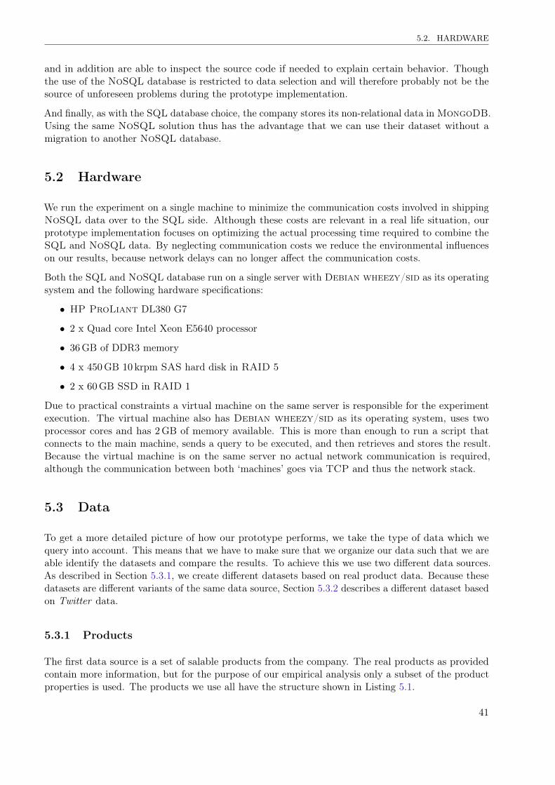
5.2. HARDWARE
and in addition are able to inspect the source code if needed to explain certain behavior. Thoughthe use of the NoSQL database is restricted to data selection and will therefore probably not be thesource of unforeseen problems during the prototype implementation.
And finally, as with the SQL database choice, the company stores its non-relational data in MongoDB.Using the same NoSQL solution thus has the advantage that we can use their dataset without amigration to another NoSQL database.
5.2 Hardware
We run the experiment on a single machine to minimize the communication costs involved in shippingNoSQL data over to the SQL side. Although these costs are relevant in a real life situation, ourprototype implementation focuses on optimizing the actual processing time required to combine theSQL and NoSQL data. By neglecting communication costs we reduce the environmental influenceson our results, because network delays can no longer affect the communication costs.
Both the SQL and NoSQL database run on a single server with Debian wheezy/sid as its operatingsystem and the following hardware specifications:
• HP ProLiant DL380 G7
• 2 x Quad core Intel Xeon E5640 processor
• 36GB of DDR3 memory
• 4 x 450GB 10 krpm SAS hard disk in RAID 5
• 2 x 60GB SSD in RAID 1
Due to practical constraints a virtual machine on the same server is responsible for the experimentexecution. The virtual machine also has Debian wheezy/sid as its operating system, uses twoprocessor cores and has 2GB of memory available. This is more than enough to run a script thatconnects to the main machine, sends a query to be executed, and then retrieves and stores the result.Because the virtual machine is on the same server no actual network communication is required,although the communication between both ‘machines’ goes via TCP and thus the network stack.
5.3 Data
To get a more detailed picture of how our prototype performs, we take the type of data which wequery into account. This means that we have to make sure that we organize our data such that we areable identify the datasets and compare the results. To achieve this we use two different data sources.As described in Section 5.3.1, we create different datasets based on real product data. Because thesedatasets are different variants of the same data source, Section 5.3.2 describes a different dataset basedon Twitter data.
5.3.1 Products
The first data source is a set of salable products from the company. The real products as providedcontain more information, but for the purpose of our empirical analysis only a subset of the productproperties is used. The products we use all have the structure shown in Listing 5.1.
41
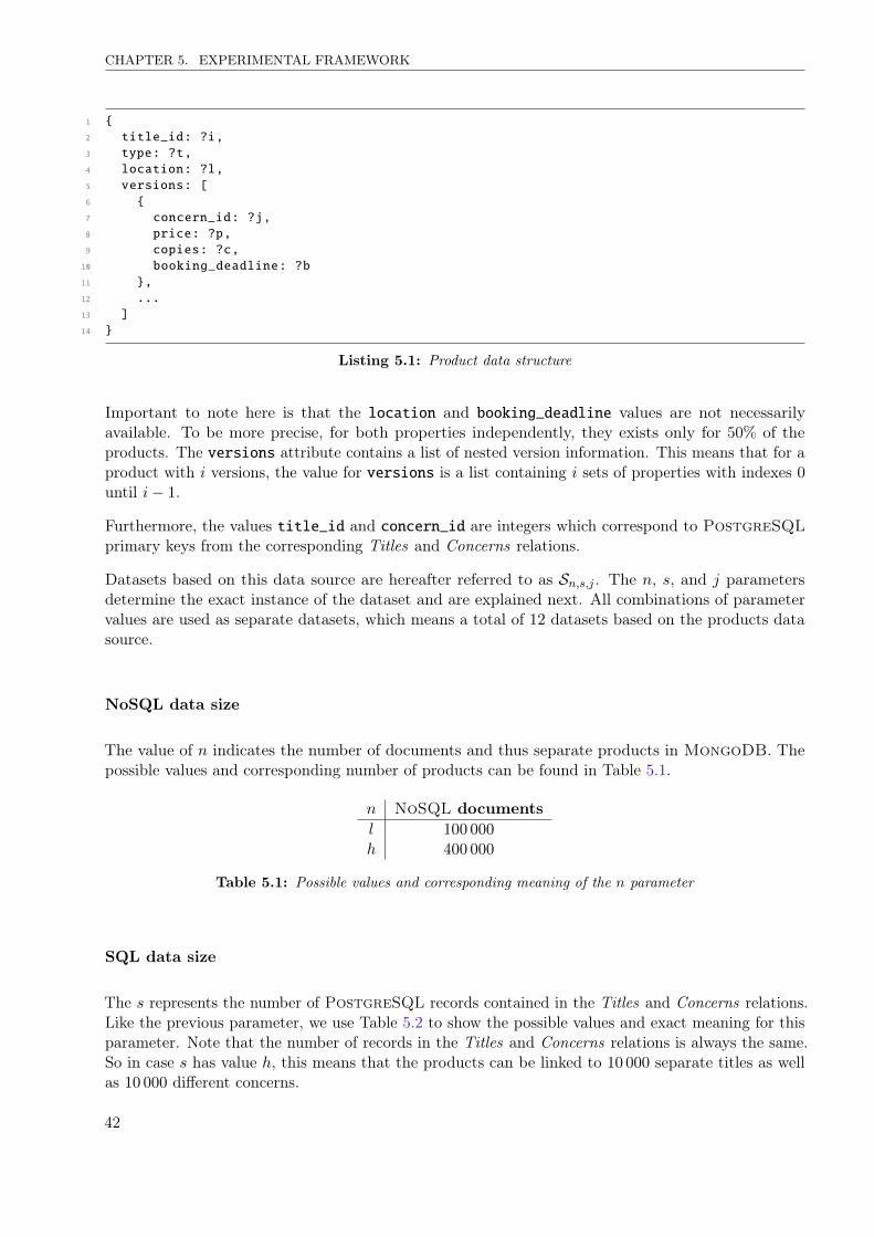
CHAPTER 5. EXPERIMENTAL FRAMEWORK
1 {2 title_id: ?i,3 type: ?t,4 location: ?l,5 versions: [6 {7 concern_id: ?j,8 price: ?p,9 copies: ?c,10 booking_deadline: ?b11 },12 ...13 ]14 }
Listing 5.1: Product data structure
Important to note here is that the location and booking_deadline values are not necessarilyavailable. To be more precise, for both properties independently, they exists only for 50% of theproducts. The versions attribute contains a list of nested version information. This means that for aproduct with i versions, the value for versions is a list containing i sets of properties with indexes 0until i− 1.
Furthermore, the values title_id and concern_id are integers which correspond to PostgreSQLprimary keys from the corresponding Titles and Concerns relations.
Datasets based on this data source are hereafter referred to as Sn,s,j . The n, s, and j parametersdetermine the exact instance of the dataset and are explained next. All combinations of parametervalues are used as separate datasets, which means a total of 12 datasets based on the products datasource.
NoSQL data size
The value of n indicates the number of documents and thus separate products in MongoDB. Thepossible values and corresponding number of products can be found in Table 5.1.
n NoSQL documentsl 100 000h 400 000
Table 5.1: Possible values and corresponding meaning of the n parameter
SQL data size
The s represents the number of PostgreSQL records contained in the Titles and Concerns relations.Like the previous parameter, we use Table 5.2 to show the possible values and exact meaning for thisparameter. Note that the number of records in the Titles and Concerns relations is always the same.So in case s has value h, this means that the products can be linked to 10 000 separate titles as wellas 10 000 different concerns.
42
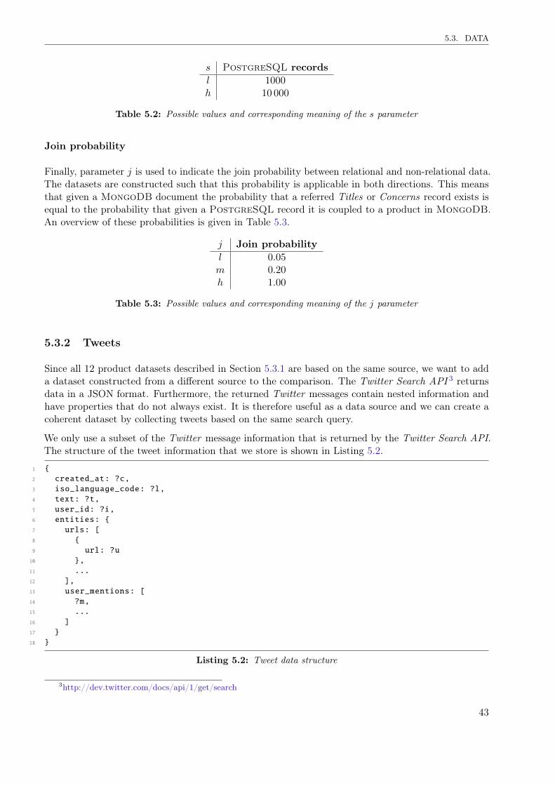
5.3. DATA
s PostgreSQL recordsl 1000h 10 000
Table 5.2: Possible values and corresponding meaning of the s parameter
Join probability
Finally, parameter j is used to indicate the join probability between relational and non-relational data.The datasets are constructed such that this probability is applicable in both directions. This meansthat given a MongoDB document the probability that a referred Titles or Concerns record exists isequal to the probability that given a PostgreSQL record it is coupled to a product in MongoDB.An overview of these probabilities is given in Table 5.3.
j Join probabilityl 0.05m 0.20h 1.00
Table 5.3: Possible values and corresponding meaning of the j parameter
5.3.2 Tweets
Since all 12 product datasets described in Section 5.3.1 are based on the same source, we want to adda dataset constructed from a different source to the comparison. The Twitter Search API 3 returnsdata in a JSON format. Furthermore, the returned Twitter messages contain nested information andhave properties that do not always exist. It is therefore useful as a data source and we can create acoherent dataset by collecting tweets based on the same search query.
We only use a subset of the Twitter message information that is returned by the Twitter Search API.The structure of the tweet information that we store is shown in Listing 5.2.
1 {2 created_at: ?c,3 iso_language_code: ?l,4 text: ?t,5 user_id: ?i,6 entities: {7 urls: [8 {9 url: ?u10 },11 ...12 ],13 user_mentions: [14 ?m,15 ...16 ]17 }18 }
Listing 5.2: Tweet data structure
3http://dev.twitter.com/docs/api/1/get/search
43
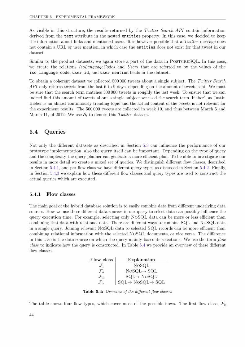
CHAPTER 5. EXPERIMENTAL FRAMEWORK
As visible in this structure, the results returned by the Twitter Search API contain informationderived from the text attribute in the nested entities property. In this case, we decided to keepthe information about links and mentioned users. It is however possible that a Twitter message doesnot contain a URL or user mention, in which case the entities does not exist for that tweet in ourdataset.
Similar to the product datasets, we again store a part of the data in PostgreSQL. In this case,we create the relations IsoLanguageCodes and Users that are referred to by the values of theiso_language_code, user_id, and user_mention fields in the dataset.
To obtain a coherent dataset we collected 500 000 tweets about a single subject. The Twitter SearchAPI only returns tweets from the last 6 to 9 days, depending on the amount of tweets sent. We mustbe sure that the search term matches 500 000 tweets in roughly the last week. To ensure that we canindeed find this amount of tweets about a single subject we used the search term ‘bieber’, as JustinBieber is an almost continuously trending topic and the actual content of the tweets is not relevant forthe experiment results. The 500 000 tweets are collected in week 10, and thus between March 5 andMarch 11, of 2012. We use St to denote this Twitter dataset.
5.4 Queries
Not only the different datasets as described in Section 5.3 can influence the performance of ourprototype implementation, also the query itself can be important. Depending on the type of queryand the complexity the query planner can generate a more efficient plan. To be able to investigate ourresults in more detail we create a mixed set of queries. We distinguish different flow classes, describedin Section 5.4.1, and per flow class we have different query types as discussed in Section 5.4.2. Finally,in Section 5.4.3 we explain how these different flow classes and query types are used to construct theactual queries which are executed.
5.4.1 Flow classes
The main goal of the hybrid database solution is to easily combine data from different underlying datasources. How we use these different data sources in our query to select data can possibly influence thequery execution time. For example, selecting only NoSQL data can be more or less efficient thancombining that data with relational data. There are different ways to combine SQL and NoSQL datain a single query. Joining relevant NoSQL data to selected SQL records can be more efficient thancombining relational information with the selected NoSQL documents, or vice versa. The differencein this case is the data source on which the query mainly bases its selections. We use the term flowclass to indicate how the query is constructed. In Table 5.4 we provide an overview of these differentflow classes.
Flow class ExplanationFi NoSQLFii NoSQL→ SQLFiii SQL→ NoSQLFiv SQL→ NoSQL→ SQL
Table 5.4: Overview of the different flow classes
The table shows four flow types, which cover most of the possible flows. The first flow class, Fi,
44
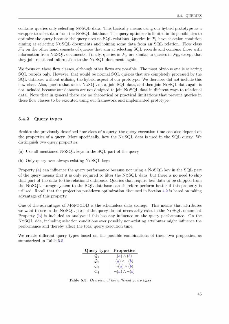
5.4. QUERIES
contains queries only selecting NoSQL data. This basically means using our hybrid prototype as awrapper to select data from the NoSQL database. The query optimizer is limited in its possibilities tooptimize the query because the query uses no SQL relations. Queries in Fii have selection conditionaiming at selecting NoSQL documents and joining some data from an SQL relation. Flow classFiii on the other hand consists of queries that aim at selecting SQL records and combine those withinformation from NoSQL documents. Finally, queries in Fiv are similar to queries in Fiii, except thatthey join relational information to the NoSQL documents again.
We focus on these flow classes, although other flows are possible. The most obvious one is selectingSQL records only. However, that would be normal SQL queries that are completely processed by theSQL database without utilizing the hybrid aspect of our prototype. We therefore did not include thisflow class. Also, queries that select NoSQL data, join SQL data, and then join NoSQL data again isnot included because our datasets are not designed to join NoSQL data in different ways to relationaldata. Note that in general there are no theoretical or practical limitations that prevent queries inthese flow classes to be executed using our framework and implemented prototype.
5.4.2 Query types
Besides the previously described flow class of a query, the query execution time can also depend onthe properties of a query. More specifically, how the NoSQL data is used in the SQL query. Wedistinguish two query properties:
(a) Use all mentioned NoSQL keys in the SQL part of the query
(b) Only query over always existing NoSQL keys
Property (a) can influence the query performance because not using a NoSQL key in the SQL partof the query means that it is only required to filter the NoSQL data, but there is no need to shipthat part of the data to the relational database. Queries that require less data to be shipped fromthe NoSQL storage system to the SQL database can therefore perform better if this property isutilized. Recall that the projection pushdown optimization discussed in Section 4.2 is based on takingadvantage of this property.
One of the advantages of MongoDB is the schemaless data storage. This means that attributeswe want to use in the NoSQL part of the query do not necessarily exist in the NoSQL document.Property (b) is included to analyze if this has any influence on the query performance. On theNoSQL side, including selection conditions over possibly non-existing attributes might influence theperformance and thereby affect the total query execution time.
We create different query types based on the possible combinations of these two properties, assummarized in Table 5.5.
Query type PropertiesQ1 (a) ∧ (b)Q2 (a) ∧ ¬(b)Q3 ¬(a) ∧ (b)Q4 ¬(a) ∧ ¬(b)
Table 5.5: Overview of the different query types
45
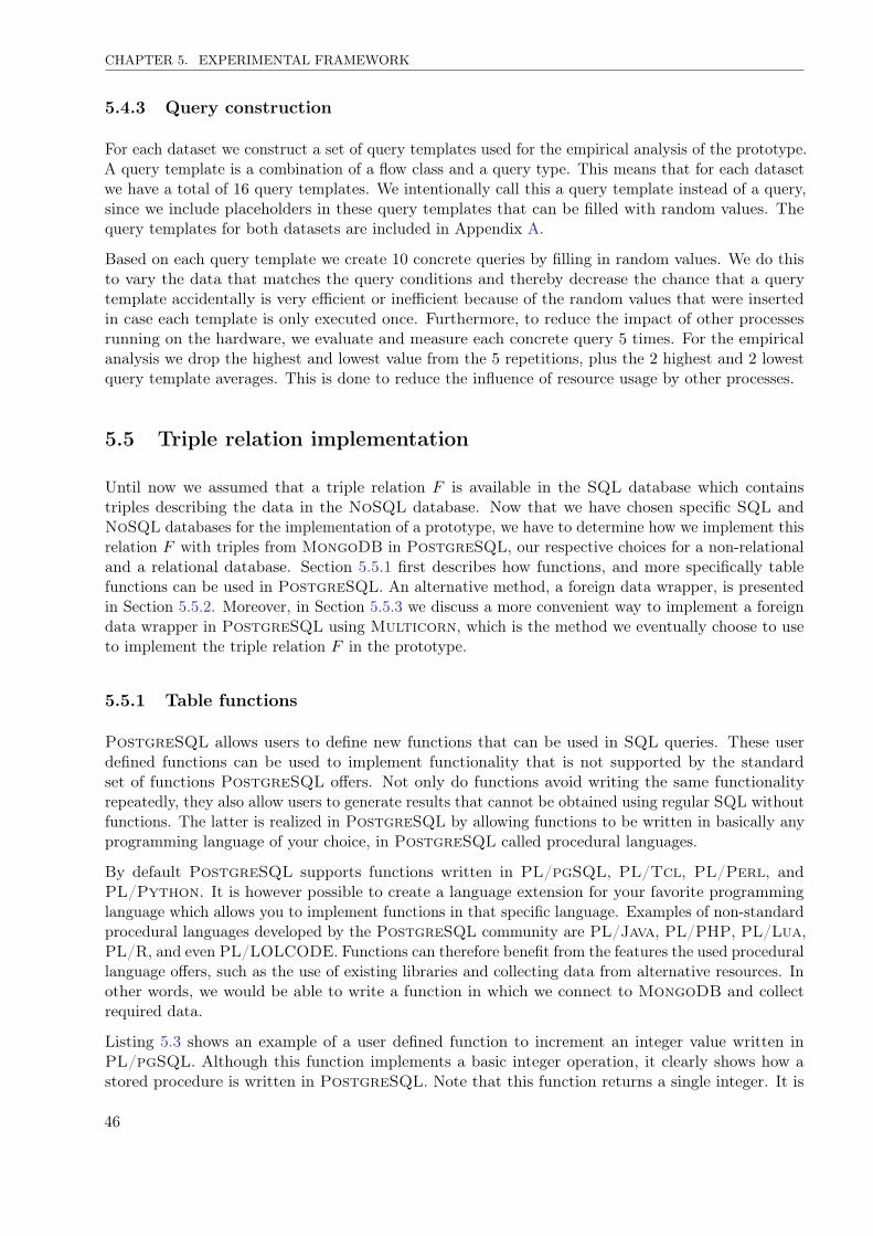
CHAPTER 5. EXPERIMENTAL FRAMEWORK
5.4.3 Query construction
For each dataset we construct a set of query templates used for the empirical analysis of the prototype.A query template is a combination of a flow class and a query type. This means that for each datasetwe have a total of 16 query templates. We intentionally call this a query template instead of a query,since we include placeholders in these query templates that can be filled with random values. Thequery templates for both datasets are included in Appendix A.
Based on each query template we create 10 concrete queries by filling in random values. We do thisto vary the data that matches the query conditions and thereby decrease the chance that a querytemplate accidentally is very efficient or inefficient because of the random values that were insertedin case each template is only executed once. Furthermore, to reduce the impact of other processesrunning on the hardware, we evaluate and measure each concrete query 5 times. For the empiricalanalysis we drop the highest and lowest value from the 5 repetitions, plus the 2 highest and 2 lowestquery template averages. This is done to reduce the influence of resource usage by other processes.
5.5 Triple relation implementation
Until now we assumed that a triple relation F is available in the SQL database which containstriples describing the data in the NoSQL database. Now that we have chosen specific SQL andNoSQL databases for the implementation of a prototype, we have to determine how we implement thisrelation F with triples from MongoDB in PostgreSQL, our respective choices for a non-relationaland a relational database. Section 5.5.1 first describes how functions, and more specifically tablefunctions can be used in PostgreSQL. An alternative method, a foreign data wrapper, is presentedin Section 5.5.2. Moreover, in Section 5.5.3 we discuss a more convenient way to implement a foreigndata wrapper in PostgreSQL using Multicorn, which is the method we eventually choose to useto implement the triple relation F in the prototype.
5.5.1 Table functions
PostgreSQL allows users to define new functions that can be used in SQL queries. These userdefined functions can be used to implement functionality that is not supported by the standardset of functions PostgreSQL offers. Not only do functions avoid writing the same functionalityrepeatedly, they also allow users to generate results that cannot be obtained using regular SQL withoutfunctions. The latter is realized in PostgreSQL by allowing functions to be written in basically anyprogramming language of your choice, in PostgreSQL called procedural languages.
By default PostgreSQL supports functions written in PL/pgSQL, PL/Tcl, PL/Perl, andPL/Python. It is however possible to create a language extension for your favorite programminglanguage which allows you to implement functions in that specific language. Examples of non-standardprocedural languages developed by the PostgreSQL community are PL/Java, PL/PHP, PL/Lua,PL/R, and even PL/LOLCODE. Functions can therefore benefit from the features the used procedurallanguage offers, such as the use of existing libraries and collecting data from alternative resources. Inother words, we would be able to write a function in which we connect to MongoDB and collectrequired data.
Listing 5.3 shows an example of a user defined function to increment an integer value written inPL/pgSQL. Although this function implements a basic integer operation, it clearly shows how astored procedure is written in PostgreSQL. Note that this function returns a single integer. It is
46
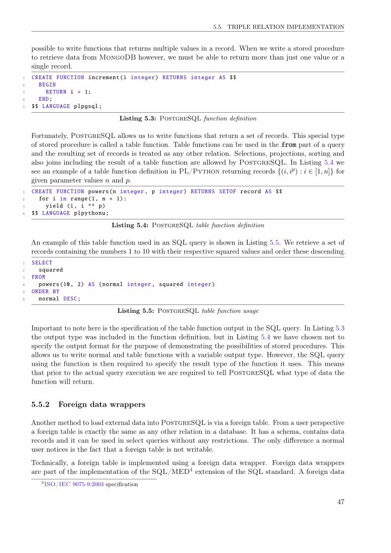
5.5. TRIPLE RELATION IMPLEMENTATION
possible to write functions that returns multiple values in a record. When we write a stored procedureto retrieve data from MongoDB however, we must be able to return more than just one value or asingle record.
1 CREATE FUNCTION increment(i integer) RETURNS integer AS $$2 BEGIN3 RETURN i + 1;4 END;5 $$ LANGUAGE plpgsql;
Listing 5.3: PostgreSQL function definition
Fortunately, PostgreSQL allows us to write functions that return a set of records. This special typeof stored procedure is called a table function. Table functions can be used in the from part of a queryand the resulting set of records is treated as any other relation. Selections, projections, sorting andalso joins including the result of a table function are allowed by PostgreSQL. In Listing 5.4 wesee an example of a table function definition in PL/Python returning records {(i, ip) : i ∈ [1, n]} forgiven parameter values n and p.
1 CREATE FUNCTION powers(n integer, p integer) RETURNS SETOF record AS $$2 for i in range(1, n + 1):3 yield (i, i ** p)4 $$ LANGUAGE plpythonu;
Listing 5.4: PostgreSQL table function definition
An example of this table function used in an SQL query is shown in Listing 5.5. We retrieve a set ofrecords containing the numbers 1 to 10 with their respective squared values and order these descending.
1 SELECT2 squared3 FROM4 powers(10, 2) AS (normal integer, squared integer)5 ORDER BY6 normal DESC;
Listing 5.5: PostgreSQL table function usage
Important to note here is the specification of the table function output in the SQL query. In Listing 5.3the output type was included in the function definition, but in Listing 5.4 we have chosen not tospecify the output format for the purpose of demonstrating the possibilities of stored procedures. Thisallows us to write normal and table functions with a variable output type. However, the SQL queryusing the function is then required to specify the result type of the function it uses. This meansthat prior to the actual query execution we are required to tell PostgreSQL what type of data thefunction will return.
5.5.2 Foreign data wrappers
Another method to load external data into PostgreSQL is via a foreign table. From a user perspectivea foreign table is exactly the same as any other relation in a database. It has a schema, contains datarecords and it can be used in select queries without any restrictions. The only difference a normaluser notices is the fact that a foreign table is not writable.
Technically, a foreign table is implemented using a foreign data wrapper. Foreign data wrappersare part of the implementation of the SQL/MED4 extension of the SQL standard. A foreign data
4ISO/IEC 9075-9:2003 specification
47
CHAPTER 5. EXPERIMENTAL FRAMEWORK
wrapper is responsible for the retrieval of data for a foreign table. It is implemented using callbackfunctions for planning, explaining and retrieving data rows for a given query. Retrieving data rows isdone using an iterator function which returns the next record according to the schema of the usedforeign table. Besides these most important functions, callback functions to begin and end a tablescan and a special rescan function have to be implemented.
Because the task of a foreign data wrapper is to manage the content of a foreign table, it closelyinteracts with the PostgreSQL internals. A foreign data wrapper must therefore be implemented inC and linked to the relevant PostgreSQL libraries. When the foreign data wrapper is compiledit can be loaded as an extension in PostgreSQL. As with procedural languages, there are foreigndata wrappers available as a PostgreSQL extension written by volunteers in the PostgreSQLcommunity.
Examples are foreign data wrappers for MySQL and Oracle, which allow a user to add a foreigntable of which the records are actually stored in another relational database located elsewhere. Moreapplicable to our use case however are foreign data wrappers for other data storage types besidesrelational databases, like Redis and CouchDB. Even less obvious data sources like LDAP, IMAPand Twitter can be accessed via available foreign data wrappers. The main challenge is to representthe external data source as a relation such that it can be accessed via queries over a foreign table.
A drawback of foreign data wrappers is that they are only recently implemented in PostgreSQL 9.1and are thus a new feature. Apparently the PostgreSQL developers deem the implementationstable enough for production. However, the immaturity could be a serious disadvantage for companiesconsidering methods to load external data into PostgreSQL. Furthermore, the current foreign datawrapper implementation in PostgreSQL does not contain all functionality specified in SQL/MED.Most importantly, only data selection is supported and foreign tables thus cannot be updated. Also,the current implementation of foreign tables in PostgreSQL is quite primitive. According to thedocumentation, the query planner does not always optimize queries using foreign tables correctly.Although no details are given in the documentation, we experienced that PostgreSQL does notalways take into account that a foreign table requires external data retrieval. Sometimes queries accessthe same foreign table literally dozens of times, resulting in an enormous communication overhead.
Foreign tables can be passed option arguments at creation, which allow the user to reuse a foreign datawrapper for several foreign tables. Most often these options are used to set connection parametersthat allow the foreign data wrapper to connect to the external data source. This can be compared totable function arguments, with the important distinction that those are specified in the query whileforeign data wrapper options have to be specified at foreign table creation.
The properties and possibilities of foreign tables seem to be about the same as table functions. Besidespragmatic arguments — unlike table functions, foreign data wrappers are actually intended to be usedfor accessing external data — there is an important aspect of foreign data wrappers which provide uswith a good reason to prefer foreign tables over table functions; the operator pushdown possibilities offoreign data wrappers. It is possible to push SQL operations like selections and projections down tothe foreign data wrapper and use this knowledge to exclude unnecessary data records from the foreigntable. In other words, foreign data wrappers can take selection and projection conditions into account,use them to select the correct subset of the external data, and thereby reduce the size of the datahandled by the SQL query.
In the C code of the foreign data wrapper the selection and projection conditions are provided via thelinked PostgreSQL libraries. The foreign data wrapper implementation can use this information torestrict the amount of data that is contained in the foreign table to which the foreign data wrapperbelongs. The selection conditions can be used to push down more advanced conditions, like the exists
48
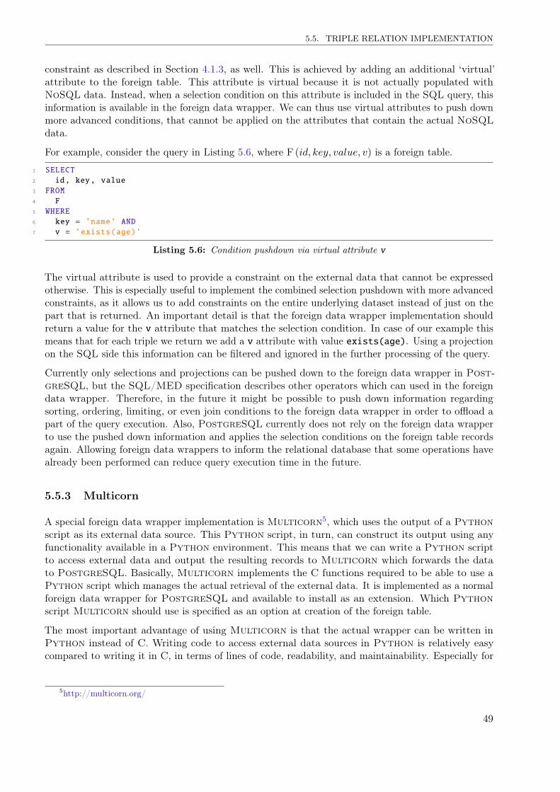
5.5. TRIPLE RELATION IMPLEMENTATION
constraint as described in Section 4.1.3, as well. This is achieved by adding an additional ‘virtual’attribute to the foreign table. This attribute is virtual because it is not actually populated withNoSQL data. Instead, when a selection condition on this attribute is included in the SQL query, thisinformation is available in the foreign data wrapper. We can thus use virtual attributes to push downmore advanced conditions, that cannot be applied on the attributes that contain the actual NoSQLdata.
For example, consider the query in Listing 5.6, where F (id, key, value, v) is a foreign table.
1 SELECT2 id, key, value3 FROM4 F5 WHERE6 key = 'name' AND7 v = 'exists(age)'
Listing 5.6: Condition pushdown via virtual attribute v
The virtual attribute is used to provide a constraint on the external data that cannot be expressedotherwise. This is especially useful to implement the combined selection pushdown with more advancedconstraints, as it allows us to add constraints on the entire underlying dataset instead of just on thepart that is returned. An important detail is that the foreign data wrapper implementation shouldreturn a value for the v attribute that matches the selection condition. In case of our example thismeans that for each triple we return we add a v attribute with value exists(age). Using a projectionon the SQL side this information can be filtered and ignored in the further processing of the query.
Currently only selections and projections can be pushed down to the foreign data wrapper in Post-greSQL, but the SQL/MED specification describes other operators which can used in the foreigndata wrapper. Therefore, in the future it might be possible to push down information regardingsorting, ordering, limiting, or even join conditions to the foreign data wrapper in order to offload apart of the query execution. Also, PostgreSQL currently does not rely on the foreign data wrapperto use the pushed down information and applies the selection conditions on the foreign table recordsagain. Allowing foreign data wrappers to inform the relational database that some operations havealready been performed can reduce query execution time in the future.
5.5.3 Multicorn
A special foreign data wrapper implementation is Multicorn5, which uses the output of a Pythonscript as its external data source. This Python script, in turn, can construct its output using anyfunctionality available in a Python environment. This means that we can write a Python scriptto access external data and output the resulting records to Multicorn which forwards the datato PostgreSQL. Basically, Multicorn implements the C functions required to be able to use aPython script which manages the actual retrieval of the external data. It is implemented as a normalforeign data wrapper for PostgreSQL and available to install as an extension. Which Pythonscript Multicorn should use is specified as an option at creation of the foreign table.
The most important advantage of using Multicorn is that the actual wrapper can be written inPython instead of C. Writing code to access external data sources in Python is relatively easycompared to writing it in C, in terms of lines of code, readability, and maintainability. Especially for
5http://multicorn.org/
49
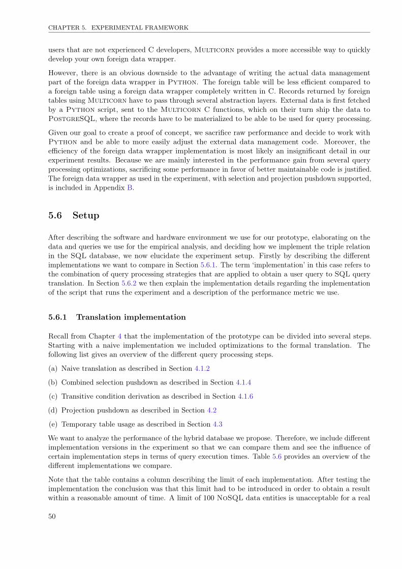
CHAPTER 5. EXPERIMENTAL FRAMEWORK
users that are not experienced C developers, Multicorn provides a more accessible way to quicklydevelop your own foreign data wrapper.
However, there is an obvious downside to the advantage of writing the actual data managementpart of the foreign data wrapper in Python. The foreign table will be less efficient compared toa foreign table using a foreign data wrapper completely written in C. Records returned by foreigntables using Multicorn have to pass through several abstraction layers. External data is first fetchedby a Python script, sent to the Multicorn C functions, which on their turn ship the data toPostgreSQL, where the records have to be materialized to be able to be used for query processing.
Given our goal to create a proof of concept, we sacrifice raw performance and decide to work withPython and be able to more easily adjust the external data management code. Moreover, theefficiency of the foreign data wrapper implementation is most likely an insignificant detail in ourexperiment results. Because we are mainly interested in the performance gain from several queryprocessing optimizations, sacrificing some performance in favor of better maintainable code is justified.The foreign data wrapper as used in the experiment, with selection and projection pushdown supported,is included in Appendix B.
5.6 Setup
After describing the software and hardware environment we use for our prototype, elaborating on thedata and queries we use for the empirical analysis, and deciding how we implement the triple relationin the SQL database, we now elucidate the experiment setup. Firstly by describing the differentimplementations we want to compare in Section 5.6.1. The term ‘implementation’ in this case refers tothe combination of query processing strategies that are applied to obtain a user query to SQL querytranslation. In Section 5.6.2 we then explain the implementation details regarding the implementationof the script that runs the experiment and a description of the performance metric we use.
5.6.1 Translation implementation
Recall from Chapter 4 that the implementation of the prototype can be divided into several steps.Starting with a naive implementation we included optimizations to the formal translation. Thefollowing list gives an overview of the different query processing steps.
(a) Naive translation as described in Section 4.1.2
(b) Combined selection pushdown as described in Section 4.1.4
(c) Transitive condition derivation as described in Section 4.1.6
(d) Projection pushdown as described in Section 4.2
(e) Temporary table usage as described in Section 4.3
We want to analyze the performance of the hybrid database we propose. Therefore, we include differentimplementation versions in the experiment so that we can compare them and see the influence ofcertain implementation steps in terms of query execution times. Table 5.6 provides an overview of thedifferent implementations we compare.
Note that the table contains a column describing the limit of each implementation. After testing theimplementation the conclusion was that this limit had to be introduced in order to obtain a resultwithin a reasonable amount of time. A limit of 100 NoSQL data entities is unacceptable for a real
50
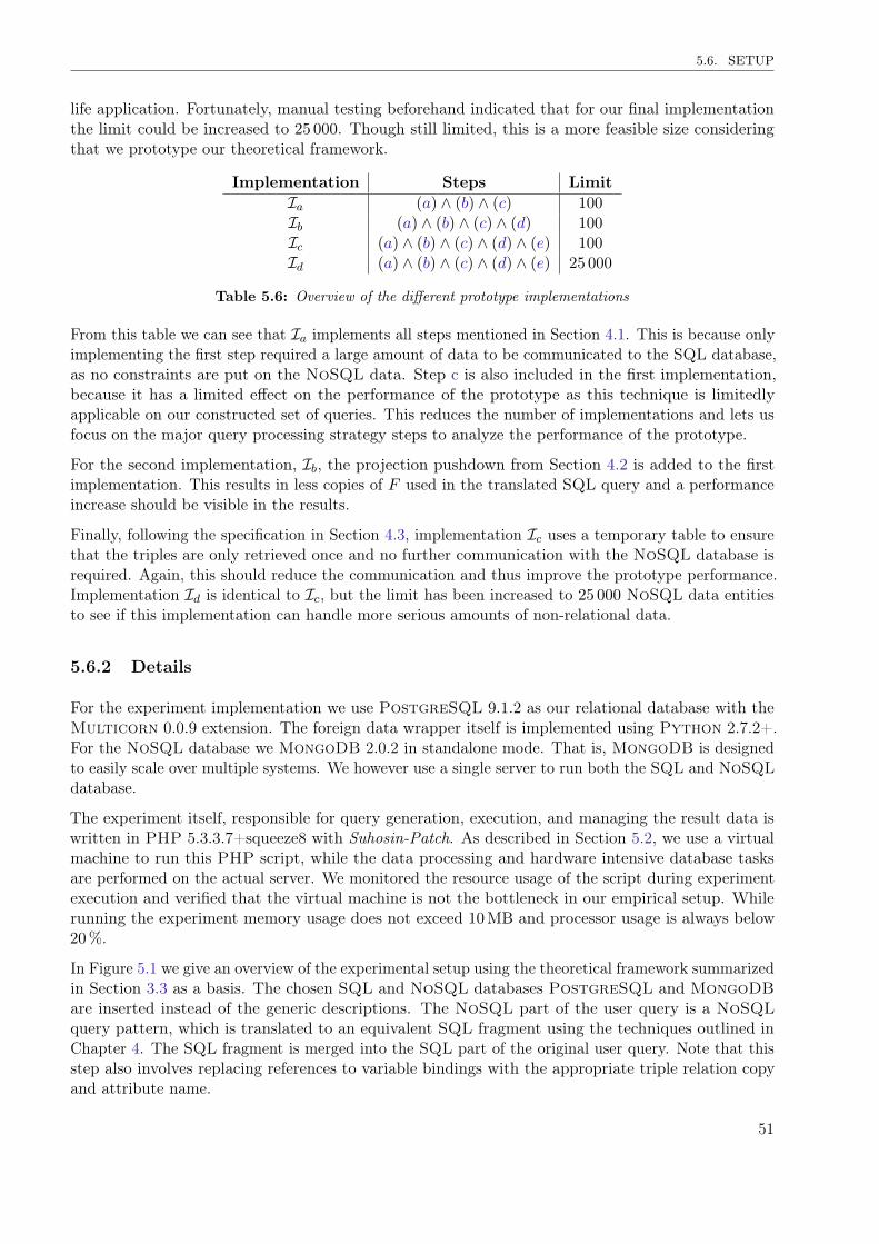
5.6. SETUP
life application. Fortunately, manual testing beforehand indicated that for our final implementationthe limit could be increased to 25 000. Though still limited, this is a more feasible size consideringthat we prototype our theoretical framework.
Implementation Steps LimitIa (a) ∧ (b) ∧ (c) 100Ib (a) ∧ (b) ∧ (c) ∧ (d) 100Ic (a) ∧ (b) ∧ (c) ∧ (d) ∧ (e) 100Id (a) ∧ (b) ∧ (c) ∧ (d) ∧ (e) 25 000
Table 5.6: Overview of the different prototype implementations
From this table we can see that Ia implements all steps mentioned in Section 4.1. This is because onlyimplementing the first step required a large amount of data to be communicated to the SQL database,as no constraints are put on the NoSQL data. Step c is also included in the first implementation,because it has a limited effect on the performance of the prototype as this technique is limitedlyapplicable on our constructed set of queries. This reduces the number of implementations and lets usfocus on the major query processing strategy steps to analyze the performance of the prototype.
For the second implementation, Ib, the projection pushdown from Section 4.2 is added to the firstimplementation. This results in less copies of F used in the translated SQL query and a performanceincrease should be visible in the results.
Finally, following the specification in Section 4.3, implementation Ic uses a temporary table to ensurethat the triples are only retrieved once and no further communication with the NoSQL database isrequired. Again, this should reduce the communication and thus improve the prototype performance.Implementation Id is identical to Ic, but the limit has been increased to 25 000 NoSQL data entitiesto see if this implementation can handle more serious amounts of non-relational data.
5.6.2 Details
For the experiment implementation we use PostgreSQL 9.1.2 as our relational database with theMulticorn 0.0.9 extension. The foreign data wrapper itself is implemented using Python 2.7.2+.For the NoSQL database we MongoDB 2.0.2 in standalone mode. That is, MongoDB is designedto easily scale over multiple systems. We however use a single server to run both the SQL and NoSQLdatabase.
The experiment itself, responsible for query generation, execution, and managing the result data iswritten in PHP 5.3.3.7+squeeze8 with Suhosin-Patch. As described in Section 5.2, we use a virtualmachine to run this PHP script, while the data processing and hardware intensive database tasksare performed on the actual server. We monitored the resource usage of the script during experimentexecution and verified that the virtual machine is not the bottleneck in our empirical setup. Whilerunning the experiment memory usage does not exceed 10MB and processor usage is always below20%.
In Figure 5.1 we give an overview of the experimental setup using the theoretical framework summarizedin Section 3.3 as a basis. The chosen SQL and NoSQL databases PostgreSQL and MongoDBare inserted instead of the generic descriptions. The NoSQL part of the user query is a NoSQLquery pattern, which is translated to an equivalent SQL fragment using the techniques outlined inChapter 4. The SQL fragment is merged into the SQL part of the original user query. Note that thisstep also involves replacing references to variable bindings with the appropriate triple relation copyand attribute name.
51
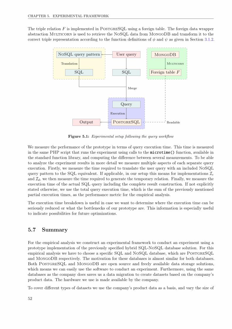
CHAPTER 5. EXPERIMENTAL FRAMEWORK
The triple relation F is implemented in PostgreSQL using a foreign table. The foreign data wrapperabstraction Multicorn is used to retrieve the NoSQL data from MongoDB and transform it to thecorrect triple representation according to the function definitions of φ and ψ as given in Section 3.1.2.
User query
SQL
NoSQL query pattern
SQL
Translation
Query
Merge
MongoDB
Foreign table F
Multicorn
PostgreSQL
Execution
ReadableOutput
Figure 5.1: Experimental setup following the query workflow
We measure the performance of the prototype in terms of query execution time. This time is measuredin the same PHP script that runs the experiment using calls to the microtime() function, available inthe standard function library, and computing the difference between several measurements. To be ableto analyze the experiment results in more detail we measure multiple aspects of each separate queryexecution. Firstly, we measure the time required to translate the user query with an included NoSQLquery pattern to the SQL equivalent. If applicable, in our setup this means for implementations Icand Id, we then measure the time required to generate the temporary relation. Finally, we measure theexecution time of the actual SQL query including the complete result construction. If not explicitlystated otherwise, we use the total query execution time, which is the sum of the previously mentionedpartial execution times, as the performance metric for the empirical analysis.
The execution time breakdown is useful in case we want to determine where the execution time can beseriously reduced or what the bottlenecks of our prototype are. This information is especially usefulto indicate possibilities for future optimizations.
5.7 Summary
For the empirical analysis we construct an experimental framework to conduct an experiment using aprototype implementation of the previously specified hybrid SQL-NoSQL database solution. For thisempirical analysis we have to choose a specific SQL and NoSQL database, which are PostgreSQLand MongoDB respectively. The motivation for these databases is almost similar for both databases.Both PostgreSQL and MongoDB are open source and freely available data storage solutions,which means we can easily use the software to conduct an experiment. Furthermore, using the samedatabases as the company does saves us a data migration to create datasets based on the company’sproduct data. The hardware we use is made available by the company.
To cover different types of datasets we use the company’s product data as a basis, and vary the size of
52
5.7. SUMMARY
the NoSQL dataset, the size of the SQL dataset, and the join probability. For each combinationsof these variables a dataset is generated. Combined with a single Twitter dataset this leads to 13different datasets. Likewise, we create a set of queries that covers multiple flow classes and severalquery types within each flow class. In total, we have 16 query templates. Each template containsplaceholders for which constant values can be included. Each query template is filled 10 times withrandom values, and each of these 10 concrete queries is executed 5 times.
The triple relation F is implemented using Multicorn, a foreign data wrapper abstraction whichallows us to write the code to retrieve the external data in Python. To run the generated queries we usea PHP script that executes all queries consecutively. The performance metric is the query executiontime, which we break down into smaller pieces to be able to analyze it in more detail if desired. Wecompare 3 different implementations that have other sets of query processing strategies included in theimplementation. A fourth implementation is equal to the third implementation, but has an increasedlimit on the number of NoSQL results. Not only have we addressed Task 3 in this chapter, we alsodescribed the experimental environment in which the implemented prototype is analyzed.
53

6Empirical analysis
The experimental framework we created is used to conduct an experiment as explained in the previouschapter and as required to complete Task 4. In this chapter we analyze the results and thereby mainlyfocus on the impact of optimization strategies we described in Chapter 4. Furthermore, we try toindicate where the bottlenecks are in the prototype implementation so that these can be investigatedand optimized in future implementations.
We start our empirical analysis by looking at a global overview of the performance of differentimplementations in Section 6.1. This gives a global overview of how each implementation performscompared to the other implementations. Then, in Section 6.2 we investigate the base implementationin more detail to see how the results are built up. In Section 6.3 we check if the projection pushdownstrategy can indeed increase the prototype performance, and we do the same for the temporary tableintroduced to minimize communication between NoSQL and SQL in Section 6.4.
Because we had to limit the number of NoSQL results in the base implementation to 100 documents,we compare implementations Ic and Id to see if the NoSQL limit can be increased when all queryprocessing strategies are applied. Recall that Id is equal to Ic, except that the NoSQL data limit is setto 25 000 instead of 100. In Section 6.5 we therefore compare the performance of both implementations.This comparison shows the impact of more NoSQL data that has to be shipped to the SQL database,and might therefore indicate possible future optimization opportunities. Section 6.6 briefly summarizesthe most important experiment results.
6.1 Result overview
In Section 5.6.1 we outlined the different prototype implementations used in the empirical analysis tocompare the impact of different query processing strategies. There are three different implementations,Ia, Ib, and Ic, that we investigate. Respectively, this are the base implementations, adding theprojection pushdown to that, and finally also applying the temporary table strategy. The fourthimplementation, Id, has another NoSQL data limit and is only included to investigate the feasibilityof the final implementation in a more realistic setting.
For each implementation we have executed a comparable set of queries as described in Section 5.4.3.Recall that we fill each of the 16 query templates 10 times with different values, and run the resultingconcrete queries 5 times each. To reduce the influence of external factors, like the server load andavailability of resources, we exclude the highest and lowest values for these 5 results. We take the
55
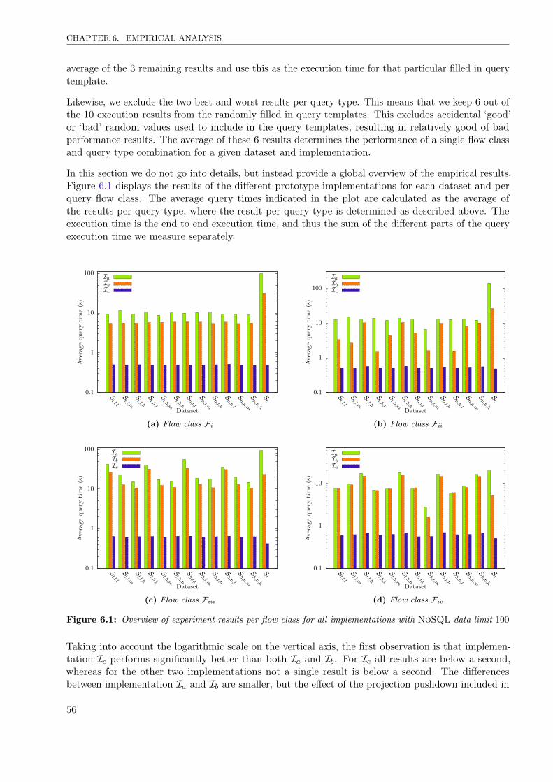
CHAPTER 6. EMPIRICAL ANALYSIS
average of the 3 remaining results and use this as the execution time for that particular filled in querytemplate.
Likewise, we exclude the two best and worst results per query type. This means that we keep 6 out ofthe 10 execution results from the randomly filled in query templates. This excludes accidental ‘good’or ‘bad’ random values used to include in the query templates, resulting in relatively good of badperformance results. The average of these 6 results determines the performance of a single flow classand query type combination for a given dataset and implementation.
In this section we do not go into details, but instead provide a global overview of the empirical results.Figure 6.1 displays the results of the different prototype implementations for each dataset and perquery flow class. The average query times indicated in the plot are calculated as the average ofthe results per query type, where the result per query type is determined as described above. Theexecution time is the end to end execution time, and thus the sum of the different parts of the queryexecution time we measure separately.
0.1
1
10
100
Sl,l,l
Sl,l,m
Sl,l,h
Sl,h,l
Sl,h,m
Sl,h,h
Sh,l,l
Sh,l,m
Sh,l,h
Sh,h,l
Sh,h,m
Sh,h,h
St
Average
querytime(s)
Dataset
IaIbIc
(a) Flow class Fi
0.1
1
10
100
Sl,l,l
Sl,l,m
Sl,l,h
Sl,h,l
Sl,h,m
Sl,h,h
Sh,l,l
Sh,l,m
Sh,l,h
Sh,h,l
Sh,h,m
Sh,h,h
St
Average
querytime(s)
Dataset
IaIbIc
(b) Flow class Fii
0.1
1
10
100
Sl,l,l
Sl,l,m
Sl,l,h
Sl,h,l
Sl,h,m
Sl,h,h
Sh,l,l
Sh,l,m
Sh,l,h
Sh,h,l
Sh,h,m
Sh,h,h
St
Average
querytime(s)
Dataset
IaIbIc
(c) Flow class Fiii
0.1
1
10
Sl,l,l
Sl,l,m
Sl,l,h
Sl,h,l
Sl,h,m
Sl,h,h
Sh,l,l
Sh,l,m
Sh,l,h
Sh,h,l
Sh,h,m
Sh,h,h
St
Average
querytime(s)
Dataset
IaIbIc
(d) Flow class Fiv
Figure 6.1: Overview of experiment results per flow class for all implementations with NoSQL data limit 100
Taking into account the logarithmic scale on the vertical axis, the first observation is that implemen-tation Ic performs significantly better than both Ia and Ib. For Ic all results are below a second,whereas for the other two implementations not a single result is below a second. The differencesbetween implementation Ia and Ib are smaller, but the effect of the projection pushdown included in
56
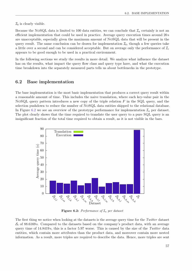
6.2. BASE IMPLEMENTATION
Ib is clearly visible.
Because the NoSQL data is limited to 100 data entities, we can conclude that Ia certainly is not anefficient implementation that could be used in practice. Average query execution times around 20 sare unacceptable, especially given the maximum amount of NoSQL data that will be present in thequery result. The same conclusion can be drawn for implementation Ib, though a few queries takea little over a second and can be considered acceptable. But on average only the performance of Icappears to be good enough to be used in a practical environment.
In the following sections we study the results in more detail. We analyze what influence the datasethas on the results, what impact the query flow class and query type have, and what the executiontime breakdown into the separately measured parts tells us about bottlenecks in the prototype.
6.2 Base implementation
The base implementation is the most basic implementation that produces a correct query result withina reasonable amount of time. This includes the naive translation, where each key-value pair in theNoSQL query pattern introduces a new copy of the triple relation F in the SQL query, and theselection pushdown to reduce the number of NoSQL data entities shipped to the relational database.In Figure 6.2 we see an overview of the prototype performance for implementation Ia per dataset.The plot clearly shows that the time required to translate the user query to a pure SQL query is aninsignificant fraction of the total time required to obtain a result, as it is not visible in the bars.
0
10
20
30
40
50
60
70
80
90
Sl,l,l
Sl,l,m
Sl,l,h
Sl,h,l
Sl,h,m
Sl,h,h
Sh,l,l
Sh,l,m
Sh,l,h
Sh,h,l
Sh,h,m
Sh,h,h
St
Average
querytime(s)
Dataset
TranslationExecution
Figure 6.2: Performance of Ia per dataset
The first thing we notice when looking at the datasets is the average query time for the Twitter datasetSt of 88.6169 s. Compared to the datasets based on the company’s product data, with an averagequery time of 14.8419 s, this is a factor 5.97 worse. This is caused by the size of the Twitter dataentities, which contain more attributes than the product data, and moreover contain more nestedinformation. As a result, more triples are required to describe the data. Hence, more triples are sent
57
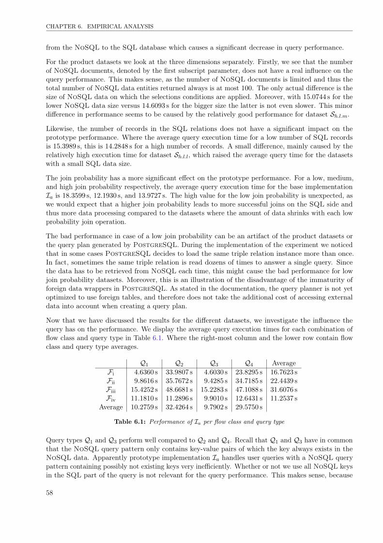
CHAPTER 6. EMPIRICAL ANALYSIS
from the NoSQL to the SQL database which causes a significant decrease in query performance.
For the product datasets we look at the three dimensions separately. Firstly, we see that the numberof NoSQL documents, denoted by the first subscript parameter, does not have a real influence on thequery performance. This makes sense, as the number of NoSQL documents is limited and thus thetotal number of NoSQL data entities returned always is at most 100. The only actual difference is thesize of NoSQL data on which the selections conditions are applied. Moreover, with 15.0744 s for thelower NoSQL data size versus 14.6093 s for the bigger size the latter is not even slower. This minordifference in performance seems to be caused by the relatively good performance for dataset Sh.l.m.
Likewise, the number of records in the SQL relations does not have a significant impact on theprototype performance. Where the average query execution time for a low number of SQL recordsis 15.3989 s, this is 14.2848 s for a high number of records. A small difference, mainly caused by therelatively high execution time for dataset Sh.l.l, which raised the average query time for the datasetswith a small SQL data size.
The join probability has a more significant effect on the prototype performance. For a low, medium,and high join probability respectively, the average query execution time for the base implementationIa is 18.3599 s, 12.1930 s, and 13.9727 s. The high value for the low join probability is unexpected, aswe would expect that a higher join probability leads to more successful joins on the SQL side andthus more data processing compared to the datasets where the amount of data shrinks with each lowprobability join operation.
The bad performance in case of a low join probability can be an artifact of the product datasets orthe query plan generated by PostgreSQL. During the implementation of the experiment we noticedthat in some cases PostgreSQL decides to load the same triple relation instance more than once.In fact, sometimes the same triple relation is read dozens of times to answer a single query. Sincethe data has to be retrieved from NoSQL each time, this might cause the bad performance for lowjoin probability datasets. Moreover, this is an illustration of the disadvantage of the immaturity offoreign data wrappers in PostgreSQL. As stated in the documentation, the query planner is not yetoptimized to use foreign tables, and therefore does not take the additional cost of accessing externaldata into account when creating a query plan.
Now that we have discussed the results for the different datasets, we investigate the influence thequery has on the performance. We display the average query execution times for each combination offlow class and query type in Table 6.1. Where the right-most column and the lower row contain flowclass and query type averages.
Q1 Q2 Q3 Q4 AverageFi 4.6360 s 33.9807 s 4.6030 s 23.8295 s 16.7623 sFii 9.8616 s 35.7672 s 9.4285 s 34.7185 s 22.4439 sFiii 15.4252 s 48.6681 s 15.2283 s 47.1088 s 31.6076 sFiv 11.1810 s 11.2896 s 9.9010 s 12.6431 s 11.2537 s
Average 10.2759 s 32.4264 s 9.7902 s 29.5750 s
Table 6.1: Performance of Ia per flow class and query type
Query types Q1 and Q3 perform well compared to Q2 and Q4. Recall that Q1 and Q3 have in commonthat the NoSQL query pattern only contains key-value pairs of which the key always exists in theNoSQL data. Apparently prototype implementation Ia handles user queries with a NoSQL querypattern containing possibly not existing keys very inefficiently. Whether or not we use all NoSQL keysin the SQL part of the query is not relevant for the query performance. This makes sense, because
58
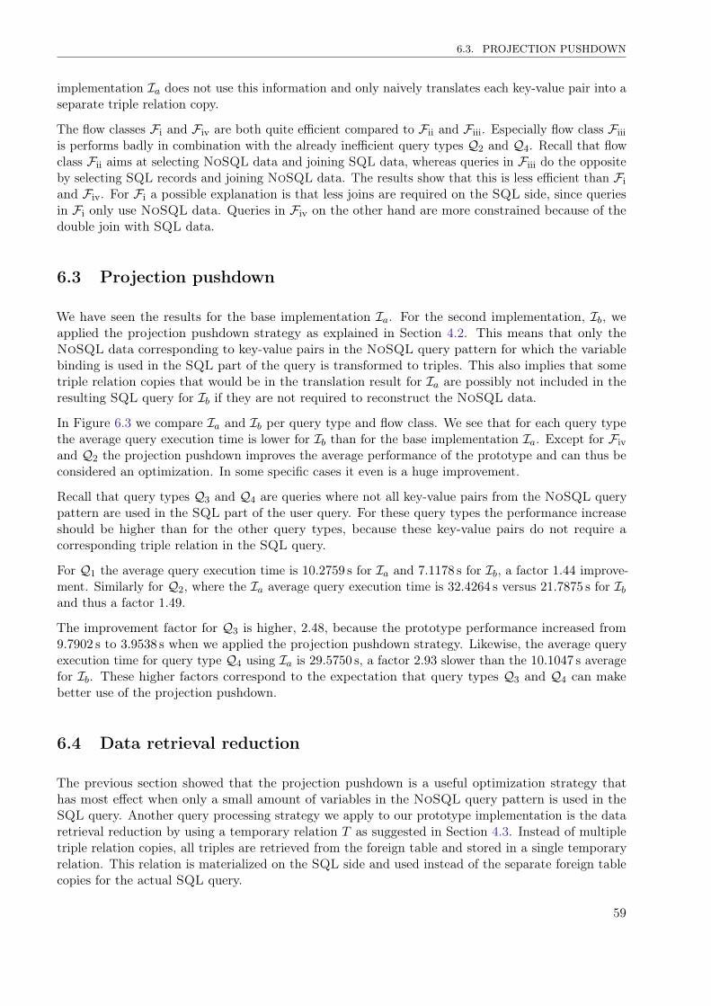
6.3. PROJECTION PUSHDOWN
implementation Ia does not use this information and only naively translates each key-value pair into aseparate triple relation copy.
The flow classes Fi and Fiv are both quite efficient compared to Fii and Fiii. Especially flow class Fiiiis performs badly in combination with the already inefficient query types Q2 and Q4. Recall that flowclass Fii aims at selecting NoSQL data and joining SQL data, whereas queries in Fiii do the oppositeby selecting SQL records and joining NoSQL data. The results show that this is less efficient than Fiand Fiv. For Fi a possible explanation is that less joins are required on the SQL side, since queriesin Fi only use NoSQL data. Queries in Fiv on the other hand are more constrained because of thedouble join with SQL data.
6.3 Projection pushdown
We have seen the results for the base implementation Ia. For the second implementation, Ib, weapplied the projection pushdown strategy as explained in Section 4.2. This means that only theNoSQL data corresponding to key-value pairs in the NoSQL query pattern for which the variablebinding is used in the SQL part of the query is transformed to triples. This also implies that sometriple relation copies that would be in the translation result for Ia are possibly not included in theresulting SQL query for Ib if they are not required to reconstruct the NoSQL data.
In Figure 6.3 we compare Ia and Ib per query type and flow class. We see that for each query typethe average query execution time is lower for Ib than for the base implementation Ia. Except for Fivand Q2 the projection pushdown improves the average performance of the prototype and can thus beconsidered an optimization. In some specific cases it even is a huge improvement.
Recall that query types Q3 and Q4 are queries where not all key-value pairs from the NoSQL querypattern are used in the SQL part of the user query. For these query types the performance increaseshould be higher than for the other query types, because these key-value pairs do not require acorresponding triple relation in the SQL query.
For Q1 the average query execution time is 10.2759 s for Ia and 7.1178 s for Ib, a factor 1.44 improve-ment. Similarly for Q2, where the Ia average query execution time is 32.4264 s versus 21.7875 s for Iband thus a factor 1.49.
The improvement factor for Q3 is higher, 2.48, because the prototype performance increased from9.7902 s to 3.9538 s when we applied the projection pushdown strategy. Likewise, the average queryexecution time for query type Q4 using Ia is 29.5750 s, a factor 2.93 slower than the 10.1047 s averagefor Ib. These higher factors correspond to the expectation that query types Q3 and Q4 can makebetter use of the projection pushdown.
6.4 Data retrieval reduction
The previous section showed that the projection pushdown is a useful optimization strategy thathas most effect when only a small amount of variables in the NoSQL query pattern is used in theSQL query. Another query processing strategy we apply to our prototype implementation is the dataretrieval reduction by using a temporary relation T as suggested in Section 4.3. Instead of multipletriple relation copies, all triples are retrieved from the foreign table and stored in a single temporaryrelation. This relation is materialized on the SQL side and used instead of the separate foreign tablecopies for the actual SQL query.
59
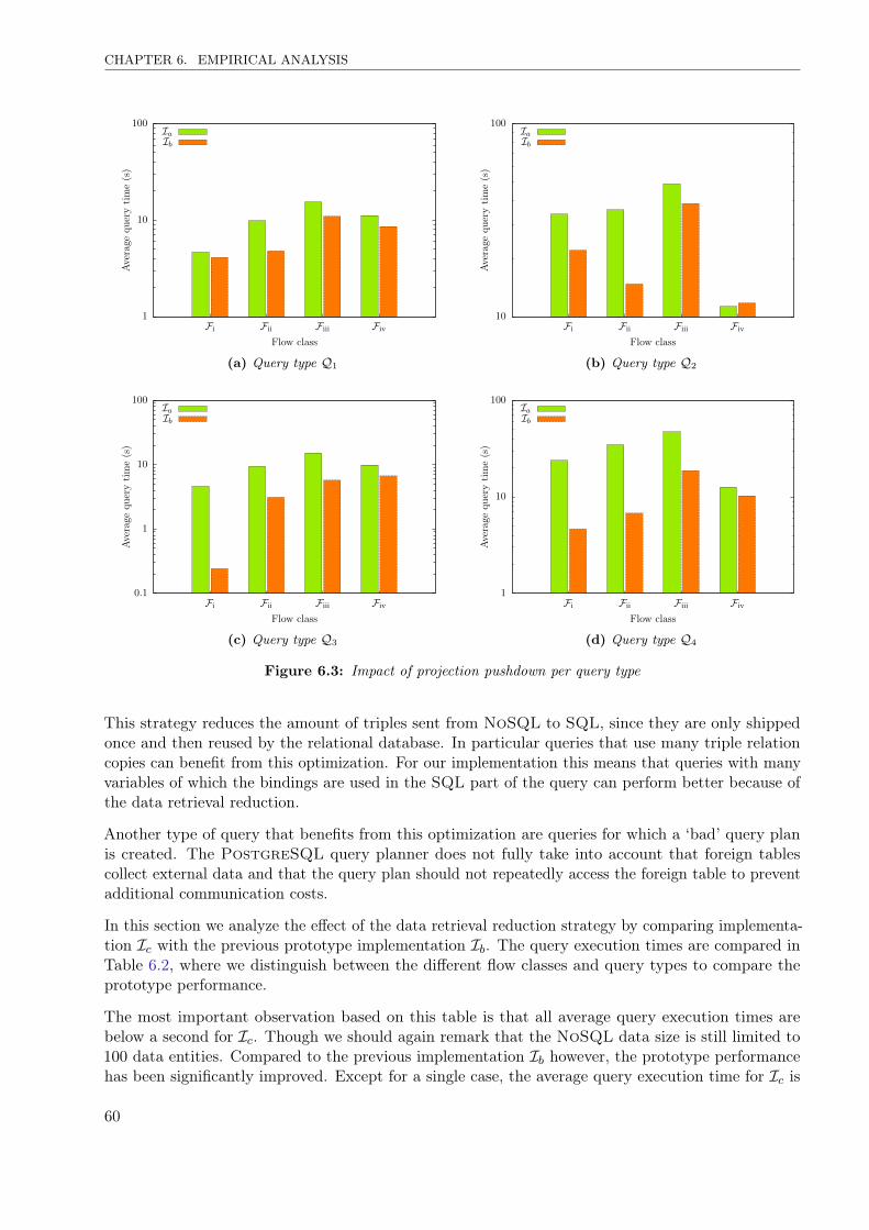
CHAPTER 6. EMPIRICAL ANALYSIS
1
10
100
Fi Fii Fiii Fiv
Average
querytime(s)
Flow class
IaIb
(a) Query type Q1
10
100
Fi Fii Fiii Fiv
Average
querytime(s)
Flow class
IaIb
(b) Query type Q2
0.1
1
10
100
Fi Fii Fiii Fiv
Average
querytime(s)
Flow class
IaIb
(c) Query type Q3
1
10
100
Fi Fii Fiii Fiv
Average
querytime(s)
Flow class
IaIb
(d) Query type Q4
Figure 6.3: Impact of projection pushdown per query type
This strategy reduces the amount of triples sent from NoSQL to SQL, since they are only shippedonce and then reused by the relational database. In particular queries that use many triple relationcopies can benefit from this optimization. For our implementation this means that queries with manyvariables of which the bindings are used in the SQL part of the query can perform better because ofthe data retrieval reduction.
Another type of query that benefits from this optimization are queries for which a ‘bad’ query planis created. The PostgreSQL query planner does not fully take into account that foreign tablescollect external data and that the query plan should not repeatedly access the foreign table to preventadditional communication costs.
In this section we analyze the effect of the data retrieval reduction strategy by comparing implementa-tion Ic with the previous prototype implementation Ib. The query execution times are compared inTable 6.2, where we distinguish between the different flow classes and query types to compare theprototype performance.
The most important observation based on this table is that all average query execution times arebelow a second for Ic. Though we should again remark that the NoSQL data size is still limited to100 data entities. Compared to the previous implementation Ib however, the prototype performancehas been significantly improved. Except for a single case, the average query execution time for Ic is
60
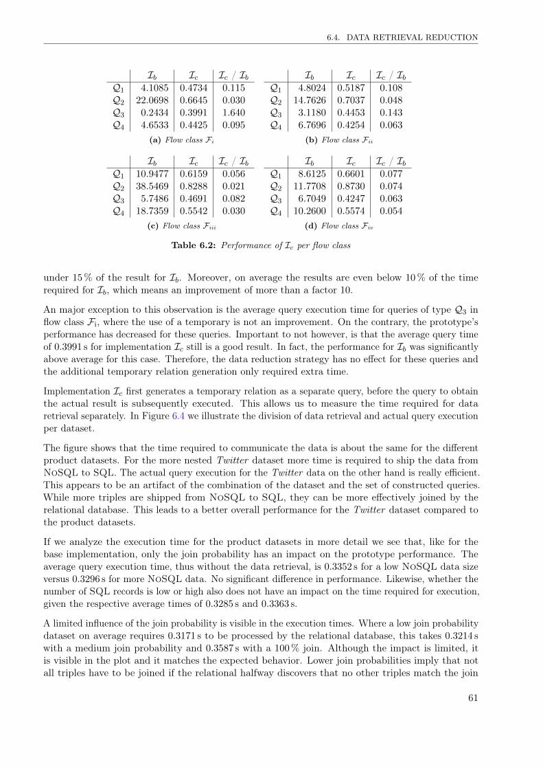
6.4. DATA RETRIEVAL REDUCTION
Ib Ic Ic / IbQ1 4.1085 0.4734 0.115Q2 22.0698 0.6645 0.030Q3 0.2434 0.3991 1.640Q4 4.6533 0.4425 0.095
(a) Flow class Fi
Ib Ic Ic / IbQ1 4.8024 0.5187 0.108Q2 14.7626 0.7037 0.048Q3 3.1180 0.4453 0.143Q4 6.7696 0.4254 0.063
(b) Flow class Fii
Ib Ic Ic / IbQ1 10.9477 0.6159 0.056Q2 38.5469 0.8288 0.021Q3 5.7486 0.4691 0.082Q4 18.7359 0.5542 0.030
(c) Flow class Fiii
Ib Ic Ic / IbQ1 8.6125 0.6601 0.077Q2 11.7708 0.8730 0.074Q3 6.7049 0.4247 0.063Q4 10.2600 0.5574 0.054
(d) Flow class Fiv
Table 6.2: Performance of Ic per flow class
under 15% of the result for Ib. Moreover, on average the results are even below 10% of the timerequired for Ib, which means an improvement of more than a factor 10.
An major exception to this observation is the average query execution time for queries of type Q3 inflow class Fi, where the use of a temporary is not an improvement. On the contrary, the prototype’sperformance has decreased for these queries. Important to not however, is that the average query timeof 0.3991 s for implementation Ic still is a good result. In fact, the performance for Ib was significantlyabove average for this case. Therefore, the data reduction strategy has no effect for these queries andthe additional temporary relation generation only required extra time.
Implementation Ic first generates a temporary relation as a separate query, before the query to obtainthe actual result is subsequently executed. This allows us to measure the time required for dataretrieval separately. In Figure 6.4 we illustrate the division of data retrieval and actual query executionper dataset.
The figure shows that the time required to communicate the data is about the same for the differentproduct datasets. For the more nested Twitter dataset more time is required to ship the data fromNoSQL to SQL. The actual query execution for the Twitter data on the other hand is really efficient.This appears to be an artifact of the combination of the dataset and the set of constructed queries.While more triples are shipped from NoSQL to SQL, they can be more effectively joined by therelational database. This leads to a better overall performance for the Twitter dataset compared tothe product datasets.
If we analyze the execution time for the product datasets in more detail we see that, like for thebase implementation, only the join probability has an impact on the prototype performance. Theaverage query execution time, thus without the data retrieval, is 0.3352 s for a low NoSQL data sizeversus 0.3296 s for more NoSQL data. No significant difference in performance. Likewise, whether thenumber of SQL records is low or high also does not have an impact on the time required for execution,given the respective average times of 0.3285 s and 0.3363 s.
A limited influence of the join probability is visible in the execution times. Where a low join probabilitydataset on average requires 0.3171 s to be processed by the relational database, this takes 0.3214 swith a medium join probability and 0.3587 s with a 100% join. Although the impact is limited, itis visible in the plot and it matches the expected behavior. Lower join probabilities imply that notall triples have to be joined if the relational halfway discovers that no other triples match the join
61
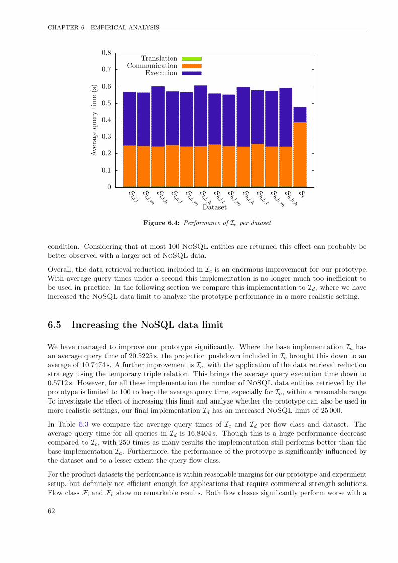
CHAPTER 6. EMPIRICAL ANALYSIS
0
0.1
0.2
0.3
0.4
0.5
0.6
0.7
0.8
Sl,l,l
Sl,l,m
Sl,l,h
Sl,h,l
Sl,h,m
Sl,h,h
Sh,l,l
Sh,l,m
Sh,l,h
Sh,h,l
Sh,h,m
Sh,h,h
St
Average
querytime(s)
Dataset
TranslationCommunication
Execution
Figure 6.4: Performance of Ic per dataset
condition. Considering that at most 100 NoSQL entities are returned this effect can probably bebetter observed with a larger set of NoSQL data.
Overall, the data retrieval reduction included in Ic is an enormous improvement for our prototype.With average query times under a second this implementation is no longer much too inefficient tobe used in practice. In the following section we compare this implementation to Id, where we haveincreased the NoSQL data limit to analyze the prototype performance in a more realistic setting.
6.5 Increasing the NoSQL data limit
We have managed to improve our prototype significantly. Where the base implementation Ia hasan average query time of 20.5225 s, the projection pushdown included in Ib brought this down to anaverage of 10.7474 s. A further improvement is Ic, with the application of the data retrieval reductionstrategy using the temporary triple relation. This brings the average query execution time down to0.5712 s. However, for all these implementation the number of NoSQL data entities retrieved by theprototype is limited to 100 to keep the average query time, especially for Ia, within a reasonable range.To investigate the effect of increasing this limit and analyze whether the prototype can also be used inmore realistic settings, our final implementation Id has an increased NoSQL limit of 25 000.
In Table 6.3 we compare the average query times of Ic and Id per flow class and dataset. Theaverage query time for all queries in Id is 16.8404 s. Though this is a huge performance decreasecompared to Ic, with 250 times as many results the implementation still performs better than thebase implementation Ia. Furthermore, the performance of the prototype is significantly influenced bythe dataset and to a lesser extent the query flow class.
For the product datasets the performance is within reasonable margins for our prototype and experimentsetup, but definitely not efficient enough for applications that require commercial strength solutions.Flow class Fi and Fii show no remarkable results. Both flow classes significantly perform worse with a
62
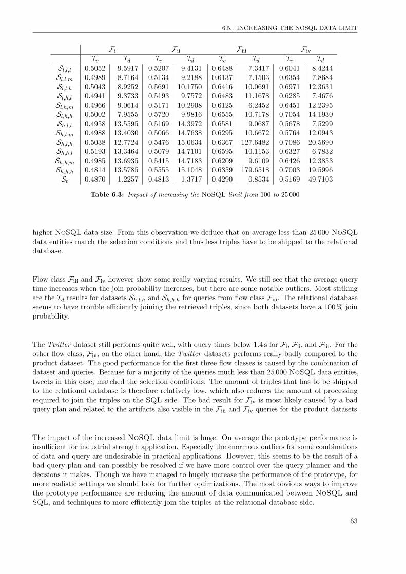
6.5. INCREASING THE NOSQL DATA LIMIT
Fi Fii Fiii FivIc Id Ic Id Ic Id Ic Id
Sl,l,l 0.5052 9.5917 0.5207 9.4131 0.6488 7.3417 0.6041 8.4244Sl,l,m 0.4989 8.7164 0.5134 9.2188 0.6137 7.1503 0.6354 7.8684Sl,l,h 0.5043 8.9252 0.5691 10.1750 0.6416 10.0691 0.6971 12.3631Sl,h,l 0.4941 9.3733 0.5193 9.7572 0.6483 11.1678 0.6285 7.4676Sl,h,m 0.4966 9.0614 0.5171 10.2908 0.6125 6.2452 0.6451 12.2395Sl,h,h 0.5002 7.9555 0.5720 9.9816 0.6555 10.7178 0.7054 14.1930Sh,l,l 0.4958 13.5595 0.5169 14.3972 0.6581 9.0687 0.5678 7.5299Sh,l,m 0.4988 13.4030 0.5066 14.7638 0.6295 10.6672 0.5764 12.0943Sh,l,h 0.5038 12.7724 0.5476 15.0634 0.6367 127.6482 0.7086 20.5690Sh,h,l 0.5193 13.3464 0.5079 14.7101 0.6595 10.1153 0.6327 6.7832Sh,h,m 0.4985 13.6935 0.5415 14.7183 0.6209 9.6109 0.6426 12.3853Sh,h,h 0.4814 13.5785 0.5555 15.1048 0.6359 179.6518 0.7003 19.5996St 0.4870 1.2257 0.4813 1.3717 0.4290 0.8534 0.5169 49.7103
Table 6.3: Impact of increasing the NoSQL limit from 100 to 25 000
higher NoSQL data size. From this observation we deduce that on average less than 25 000 NoSQLdata entities match the selection conditions and thus less triples have to be shipped to the relationaldatabase.
Flow class Fiii and Fiv however show some really varying results. We still see that the average querytime increases when the join probability increases, but there are some notable outliers. Most strikingare the Id results for datasets Sh.l.h and Sh,h,h for queries from flow class Fiii. The relational databaseseems to have trouble efficiently joining the retrieved triples, since both datasets have a 100% joinprobability.
The Twitter dataset still performs quite well, with query times below 1.4 s for Fi, Fii, and Fiii. For theother flow class, Fiv, on the other hand, the Twitter datasets performs really badly compared to theproduct dataset. The good performance for the first three flow classes is caused by the combination ofdataset and queries. Because for a majority of the queries much less than 25 000 NoSQL data entities,tweets in this case, matched the selection conditions. The amount of triples that has to be shippedto the relational database is therefore relatively low, which also reduces the amount of processingrequired to join the triples on the SQL side. The bad result for Fiv is most likely caused by a badquery plan and related to the artifacts also visible in the Fiii and Fiv queries for the product datasets.
The impact of the increased NoSQL data limit is huge. On average the prototype performance isinsufficient for industrial strength application. Especially the enormous outliers for some combinationsof data and query are undesirable in practical applications. However, this seems to be the result of abad query plan and can possibly be resolved if we have more control over the query planner and thedecisions it makes. Though we have managed to hugely increase the performance of the prototype, formore realistic settings we should look for further optimizations. The most obvious ways to improvethe prototype performance are reducing the amount of data communicated between NoSQL andSQL, and techniques to more efficiently join the triples at the relational database side.
63
CHAPTER 6. EMPIRICAL ANALYSIS
6.6 Summary
Using the experimental framework outlined in the previous chapter, we have conducted an experimentto empirically analyze the performance of our prototype and investigate the effects of the differentquery processing strategies described in Chapter 4. The main goal of the empirical analysis was tocompare the different prototype implementations and indicate possible bottlenecks which identifypossible future optimization possibilities, as stated in the description of Task 4.
From an average query execution time of 20.5225 s for our base implementation Ia, we managed toreduce this to 10.7474 s by applying the projection strategy, and even significantly improve the perfor-mance of implementation Ic by reducing the communication costs using a temporarily materializedtriple relation to an average query time of 0.5712 s.
The query execution time breakdown for the base implementation Ia already indicated that thetranslation time, to translate the user query with a NoSQL query pattern to a pure SQL query, isnegligible. The prototype is really inefficient when querying over the Twitter dataset. For the productdatasets queries using possibly non-existing NoSQL data attributes are less efficient. Similarly, queriesin flow class Fiii, where we mainly select SQL data and join NoSQL information, are less suitable forour base prototype implementation.
With the additional query processing strategy implemented in Ib we were able to improve theperformance of the prototype. Especially queries for which many triple relation copies are not requiredfor the reconstruction of the NoSQL data can benefit from the projection pushdown. When wealso implement the data retrieval reduction strategy using a temporary relation, the average queryexecution time is significantly reduced and on average all queries are answered within a second forprototype implementation Ic.
When we increase the limit on the number of NoSQL data entities retrieved by the prototype however,the performance of implementation Id decreases. With average query times of almost 17 s however,further optimizations are required to obtain an acceptable performance in a more realistic settingregarding the amount of NoSQL data the prototype can handle. The results indicate that moreefficient joins and additional control over the SQL query plan could improve the performance of theprototype.
64
7Conclusions
Our empirical analysis showed that implementing a practical prototype based on the constructed,non-trivial, and generically applicable theoretical framework is possible and that we have developed ahybrid system to access SQL and NoSQL data via an intermediate triple representation of the data.The analysis also showed that there is enough space for future improvement. This chapter concludesthis report by summarizing what we have achieved and to what extent we managed to perform thefour tasks specified in Section 1.2. The first two tasks were aimed at constructing a theoretical solutionto bridge the gap between SQL and NoSQL. How we achieved this is summarized in Section 7.1.
The practical tasks, the last two, are discussed in Section 7.2. We implemented a prototype of theproposed theoretical solution and empirically analyzed its performance. The main results and pointersfor future improvement are summed up, followed by a more detailed discussion on suggestions forfuture work in Section 7.3.
7.1 Summary of theoretical results
To bridge the gap between SQL and NoSQL, we created a hybrid database that acts as a single,read-only database that can be used to retrieve combined relational and non-relational data. Developersusing the abstraction layer do not have to worry about the underlying data separation, except whichdata is stored where. The NoSQL data is transformed to a triple representation. This allows us tomodel arbitrary data, as we have shown by providing a transformation from arbitrary nested key-valuestructures to triples.
These triples are incorporated in the relational database via a virtual triple relation F . Disregardingthe implementation details, this relation retrieves the NoSQL data in triple format when it is accessedby the developer. The triples returned by the introduced triple relation F can be considered key-valuepairs, where an identifier in the triple is used to connect the key-value pairs which belong to the sameNoSQL data entity. Nested data can be modeled via a key-value pair for which the value is equal tothe identifiers of all underlying nested attributes.
On the SQL side we then need to reconstruct the NoSQL data. To achieve this, we can use theidentifiers in the triples. Via a series of self joins with the correct join conditions the developer is ableto reconstruct the nested NoSQL data in an ordinary SQL query. However, this reconstruction is atedious task and we wanted to create a convenient method to combine SQL and NoSQL data. Wetherefore introduce an extension to SQL that includes a NoSQL query pattern in a normal SQL query.
65
CHAPTER 7. CONCLUSIONS
This NoSQL query pattern describes the conditions on the NoSQL data and can furthermore bedirectly translated to an equivalent pure SQL query with all required joins included. Bound variablesaccording to the NoSQL query pattern can be used in other parts of the SQL to combine the SQLand NoSQL data.
The result of this work is a theoretical framework to bridge SQL and NoSQL. The developer sends aquery containing a NoSQL query pattern. This pattern is translated to an equivalent SQL fragmentthat correctly joins the NoSQL triples retrieved from copies of the triple relation F . The triplescontained in relation F represent the NoSQL data we wanted to query. The result is a pure SQLquery which can be executed like any other query. When the query is executed relation F retrievesthe NoSQL data from the non-relational storage system and the data is automatically included in thequery result as described by the user query.
A naive translation of the NoSQL query pattern to SQL causes significant overhead. We thereforepropose some non-trivial and more advanced processing strategies to optimize the translation. Thesequery processing strategies are mainly aimed at reducing the amount of triples shipped from theNoSQL database to the relational database. This is achieved by pushing down selection and projectionconditions to the NoSQL database instead of communicating the entire NoSQL database in tripleformat. Furthermore, we propose a strategy to combine all triples in a single relation that is materializedby the relational database prior to query execution. This reduces the communication cost to a singleretrieve operation, after which the SQL database is able to execute the query using this temporarilystored triple relation with all required NoSQL data.
This framework is constructed independent of the underlying SQL and NoSQL databases. Usingrelational algebra notation and not going into implementation details regarding triple relation F , weare able to provide a generically applicable theoretical framework to bridge SQL and NoSQL. Wehave thereby solved Task 1 and Task 2, the first two tasks we had to address to provide an appropriatesolution to bridge SQL and NoSQL.
7.2 Summary of practical results
To cover Task 3 and Task 4, the second two tasks of our general problem, we have performed athorough empirical analysis of the developed theoretical framework using a prototype implementation.In contrast to the theoretical framework, the prototype implementation obviously cannot be constructedin a database-oblivious way. We therefore have chosen to use PostgreSQL and MongoDB as theunderlying relational and non-relational databases for the experiment. To incorporate the NoSQL datain triple format in the relational database, we used the Multicorn foreign data wrapper abstraction.This allowed us to create a foreign table in PostgreSQL that can be used like any other relation inPostgreSQL. Except when a foreign table is used in a query, the records are actually retrieved onthe fly from the external data source. In our case, the MongoDB data is transformed to its triplerepresentation and shipped to the relational database.
To investigate the prototype performance in more detail, we have constructed multiple datasets. Usingdifferent data sources to create the dataset, varying the amount of SQL records, the size of the NoSQLdata, and the join probability between the relational and non-relational data, we generated 13 differentdatasets used for the empirical analysis. Likewise, we constructed an extensive set of query templatescovering different scenarios. For four different flow classes we generated four query templates suchthat they cover all combinations of interesting properties in the NoSQL query pattern.
Using this experimental framework we compared different implementation versions of the prototype.Firstly, we analyzed the base implementation with only the selection pushdown strategy applied. To
66
7.3. FUTURE WORK
investigate the effect of the projection pushdown we included this strategy in a second implementationwhich we can compare to the base implementation. Finally, we also applied the data reduction strategyusing the materialized temporary relation to check if this indeed significantly reduces the amountof NoSQL data that is shipped to the SQL database and thereby improves the performance of theprototype.
The empirical analysis indicated that reducing the amount of triples shipped from NoSQL to SQLindeed results in a lower average query execution time. Firstly, the projection pushdown improves theperformance of the prototype with a factor 1.9, on average almost halving the time required to geta query result. Moreover, the use temporary relation further reduced the total size of the data sentfrom MongoDB to PostgreSQL, which meant another performance improvement with a factor18.8 compared to the second implementation.
When we increased the limit on the amount of NoSQL data, which we had set to get a practicableexperiment to compare the optimizations to the base implementation, we noticed that the averagequery time increased as a result of the extra communication involved and the additional processingrequired to join this larger NoSQL triple relation. While feasible for our experiment, the performanceof the final solution with an acceptable limit on the NoSQL data is not good enough to be applicablein a business environment where fast data retrieval is required. We did however notice that furtherimprovement of the prototype can be achieved by optimizing the joins of the triple relation and havingmore control over the query plan and execution.
Summarizing, the theoretical analysis showed that we have implemented a prototype of the designedtheoretical framework that successfully bridges the gap between SQL and NoSQL. However, therestill is enough space for further improvement and additional research is required in order to obtain anindustrial strength hybrid SQL-NoSQL solution.
7.3 Future work
The approach we proposed, specified, formalized, and empirically analyzed using a prototype is farfrom the ultimate solution to bridge SQL and NoSQL. Besides completely different approaches, evenwithin the same solution direction there are plenty of possibilities to narrow the gap between SQLand NoSQL by improving the performance of the hybrid database to bridge both data storage worlds.This section provides some suggestions for possible follow-up research based on our solution.
Our prototype implementation can be further optimized by reducing the amount of triples that shouldbe shipped from the NoSQL to the SQL database, as suggested in Section 7.3.1. Furthermore,Section 7.3.2 offers possible ways to more efficiently join the triples at the SQL side. On a bigger scale,we describe potential strategies to reduce the query time for more complex queries and sets of queriesin Section 7.3.3. In Section 7.3.4 we discuss run-time optimizations that could be applied duringquery execution, in contrast to our techniques that are all applied prior to query execution. Finally,Section 7.3.5 focuses on the lack of a standard NoSQL query language and covers the implications astandard hybrid query language could have on our framework.
7.3.1 Nested join reduction
A possible method to decrease the amount of data that has to be shipped from the NoSQL databaseto the SQL side is by further decreasing the number of triples required to reconstruct the NoSQLdata. In our final implementations Ic and Id, the temporary table still contains triples that are only
67
CHAPTER 7. CONCLUSIONS
used to connect different triples and are themselves not part of the NoSQL result. This is the casewhen a NoSQL query pattern contains a variable that is nested, while not all of its parents are used inthe SQL part of the user query. In our final prototype implementation, additional triples are requiredto ensure that the nested NoSQL data is correctly reconstructed.
Especially for deeply nested data, this can potentially cause that a significant portion of triples is notactually needed by the relational database. Consider the following NoSQL query pattern:
(k1 : (k2 : (. . . kn : (k : ?v) . . .)))
There are n nesting levels, with keys k1, k2, . . . , kn, until eventually we have a variable ?v for whichwe want to bind values for key k. Although only the variable binding for ?v is of interest, in our finalimplementation all n triples with nesting information are available in relation F in the SQL databaseas well. Not only are the unnecessary triples shipped to the relational database, they are also alljoined in order to mimic the NoSQL structure before eventually only using the ?v value in the rest ofthe SQL query.
In this case it is easy to see that the n triples with nesting information are not required by theSQL database. But in general, when more complicated nesting structures and additional variables inalternative paths of one of the ancestors are used, it is not trivial which triples are required and whichnot.
However, investigating this opportunity to reduce the amount of data that has to be communicated tothe relational database would certainly be worthwhile. Reducing the communication and, in this case,thereby also the number of joins could significantly improve the performance of the hybrid databasefor nested data.
7.3.2 Tuple reconstruction
Because we first transform the NoSQL data to triples to have a structured triple relation F at theSQL side, the NoSQL data is first split into different key-value pairs and later reconstructed bycorrectly joining the triples in the relational database. The flexibility these triples offer is good for ageneric NoSQL data inclusion in SQL and furthermore allows the NoSQL data to be represented asa relational table. However, an obvious disadvantage is that the data has to be reconstructed via aseries of joins.
The temporary relation F contains all triples required to achieve this reconstruction. When a largeamount of NoSQL data, in terms of triples, must be communicated to the relational database, thisresults in a giant triple relation. The self joins required to reconstruct the NoSQL data can then havea huge impact on the performance of the entire query.
One of the benefits the temporary table offers, is that its possibilities are almost similar to ‘normal’relations. For example, this provides the possibility to add indexes to F that might speed up the selfjoins. Candidate attributes would be the id, which is heavily used during the series of joins. Because aNoSQL query pattern most likely declares many keys and searches for corresponding variable bindingsfor their values, the key attribute is another possible indexing candidate.
Moreover, we can also use the information that the self joins on the F relation combines triples thatoriginate from the same NoSQL data entity. For triples at the same NoSQL query pattern nestinglevel, this can be directly derived from the fact that the join conditions states that the id values
68
7.3. FUTURE WORK
should be the same. Nested data from the same NoSQL entity however, has a separate id valuewhich is linked via the value of another triple.
Despite the different id value, these nested triples are at some point joined to the triples at anothernesting level. It can therefore be beneficial to provide this information to the SQL database, such thatthe query planner can take this into account. This can be implemented by adding an extra attributeto relation F that, in the transformation from NoSQL data to the triple representation, is filled withthe same value for each triple from the same NoSQL data entity. Often the NoSQL database willhave a data identifier available that can be used for this purpose. Otherwise, a unique identifier perdata entity can be determined during the transformation to triples.
This additional attribute of F could then be used in an additional join condition added to each selfjoin on relation F . Say we name the new attribute x, then we add the condition F1.x = F2.x if wewant to join F1 and F2. Now, regardless of whether F1 and F2 contain data at the same nesting levelin the NoSQL query pattern, the x values should be the same. Adding an index on this new attributecould increase the query performance, as the data can now also be ordered using this field to, forexample, allow a merge join on this attribute.
7.3.3 Triple relation reuse
So far, we have only considered user queries with a single NoSQL query pattern in it. Though oursolution is constructed to support multiple patterns in a single query, this functionality is not usedin the empirical analysis and not explicitly discussed in this report. Further investigation of thepossibilities and the performance impact when using more than one NoSQL query pattern in a singleuser query could provide useful insights.
User queries covering multiple triple relations also form a case where the overall performance of thefinal query can be optimized. Particularly when the same NoSQL database is used more than once, itmight be possible to combine the triples in a single triple relation to minimize the overhead introducedby connecting to an external data source. Furthermore, returned triples might be reused by eachNoSQL query pattern, which can also reduce the total amount of triples that has to be shipped fromNoSQL.
Reusing F or a subset of its triples introduces some new problems that have to be solved. We have todistinguish the triples per NoSQL query pattern in order to correctly reconstruct the NoSQL datafor each pattern. Achieving this is more complicated if triples can be reused by other patterns as well,since it then no longer belongs to a single NoSQL query pattern.
The general idea of using triples for more than one NoSQL query pattern can be taken a stepfurther. If a set of queries that is executed sequentially contains similar queries, the temporary relationgenerated for one query can possibly be reused by another query. Moreover, instead of optimizing asingle user query we can then also look at improving the performance for a given set of queries. Thatis, combining the triples required for multiple user queries in a single temporary relations can improvethe performance for the entire set of queries if this relation can be used by a multiple queries.
Note that such multi-query optimizations are closely related to other research areas like OLAP1 viewmaterialization. For large amounts of multi-dimensional data, determining which views are useful tomaterialize in order to improve the overall performance for OLAP tasks is essentially the same asdetermining what is the optimal set of triple relations to materialize given a set of user queries.
1http://www.olapcouncil.org/
69
CHAPTER 7. CONCLUSIONS
For both possible future research ideas, optimizing for more than one NoSQL query pattern per userquery and multi-query optimization, it is important to take into account that materializing triplerelations means that we have to sacrifice NoSQL data consistency. But, as for OLAP, there aresituations for which this is not a problem and in these cases applying this type of optimization couldreduce the overall query time and thereby improve the performance of the application.
7.3.4 Dynamic run-time query evaluation strategies
The query processing strategies described in Chapter 4 and implemented in our prototype all focus onthe translation from user query to pure SQL. The user query is translated prior to query execution, andall strategies treated in this report aim at optimizing this static translation. As the empirical analysisshowed, optimizing the translation can significantly improve the query performance by reducing theamount of triples required to reconstruct the NoSQL data on the relational database side.
After the translation however, the query is executed like a normal SQL query. During query evaluation,it is possible that additional constraints on the NoSQL data can be derived. For example, selectionson the relational data could restrict the set of SQL records in the query result. This informationcould be used when accessing the triple relation F to join NoSQL data to the SQL result. Triplesdescribing data that will not be joined to the SQL data, because it has been filtered out already,do not have to be shipped from NoSQL to SQL. This additional constraint, which is dynamicallyderived during query execution, could thus be used to reduce the amount of NoSQL triples that haveto be communicated between both underlying databases.
Similarly, other information that could reduce the amount of NoSQL entities that has to be sent to therelational database can become available during run-time query evaluation. Pushing these additionalconditions down to the NoSQL database during query execution improves the overall performanceof the prototype. This type of dynamic run-time strategies are a different approach at optimizingthe prototype performance and are not covered in this report. Further research to determine whichadditional constraints we can derive at run-time and how we send these new conditions to the NoSQLdatabase prior to data communication is required to practically apply this suggestion.
Building further on this idea, another possibility is to introduce query rewrite rules the query plannercan apply to better reckon with the fact that the triple relation F imports external data when it isaccessed. Rules to ensure that as much selection and projection conditions as possible can be appliedon the NoSQL data reduce the amount of triples shipped to the relational database.
Furthermore, usage of attributes from relation F can be postponed as long as possible in the queryplan. This extends the run-time period in which additional constraints can be dynamically derived andpushed down to the NoSQL database. In other words, rewrite rules can ensure that the maximumset of constraints on the triple relation are constructed and applied before the NoSQL data iscommunicated to the SQL database.
7.3.5 NoSQL query language standardization
The query language proposed in Section 3.2 includes a NoSQL query pattern in a normal SQLstatement. This way, the user is able to read and combine data from an SQL and a NoSQL source ina single query. However, a disadvantage of this query syntax is the clear separation between the SQLand NoSQL part. Although this is convenient if we want to process a query, it might still feel liketwo separate query languages merged together in a single statement.
70
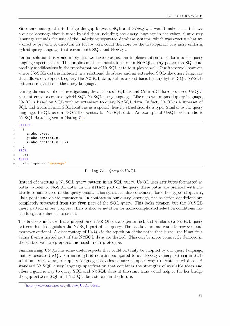
7.3. FUTURE WORK
Since our main goal is to bridge the gap between SQL and NoSQL, it would make sense to havea query language that is more hybrid than including one query language in the other. Our querylanguage reminds the user of the underlying separated database systems, which was exactly what wewanted to prevent. A direction for future work could therefore be the development of a more uniform,hybrid query language that covers both SQL and NoSQL.
For our solution this would imply that we have to adjust our implementation to conform to the querylanguage specification. This implies another translation from a NoSQL query pattern to SQL andpossibly modifications in the transformation of NoSQL data to triples as well. Our framework however,where NoSQL data is included in a relational database and an extended SQL-like query languagethat allows developers to query the NoSQL data, still is a solid basis for any hybrid SQL-NoSQLdatabase regardless of the query language.
During the course of our investigations, the authors of SQLite and CouchDB have proposed UnQL2
as an attempt to create a hybrid SQL-NoSQL query language. Like our own proposed query language,UnQL is based on SQL with an extension to query NoSQL data. In fact, UnQL is a superset ofSQL and treats normal SQL relations as a special, heavily structured data type. Similar to our querylanguage, UnQL uses a JSON-like syntax for NoSQL data. An example of UnQL, where abc isNoSQL data is given in Listing 7.1.
1 SELECT2 {3 x:abc.type,4 y:abc.content.x,5 z:abc.content.x + 506 }7 FROM8 abc9 WHERE10 abc.type == 'message'
Listing 7.1: Query in UnQL
Instead of inserting a NoSQL query pattern in an SQL query, UnQL uses attributes formatted aspaths to refer to NoSQL data. In the select part of the query these paths are prefixed with theattribute name used in the query result. This syntax is also convenient for other types of queries,like update and delete statements. In contrast to our query language, the selection conditions arecompletely separated from the from part of the SQL query. This looks cleaner, but the NoSQLquery pattern in our proposal offers a shorter notation for more complicated selection conditions likechecking if a value exists or not.
The brackets indicate that a projection on NoSQL data is performed, and similar to a NoSQL querypattern this distinguishes the NoSQL part of the query. The brackets are more subtle however, andmoreover optional. A disadvantage of UnQL is the repetition of the paths that is required if multiplevalues from a nested part of the NoSQL data are desired. This can be more compactly denoted inthe syntax we have proposed and used in our prototype.
Summarizing, UnQL has some useful aspects that could certainly be adopted by our query language,mainly because UnQL is a more hybrid notation compared to our NoSQL query pattern in SQLsolution. Vice versa, our query language provides a more compact way to treat nested data. Astandard NoSQL query language specification that combines the strengths of available ideas andoffers a generic way to query SQL and NoSQL data at the same time would help to further bridgethe gap between SQL and NoSQL data storage in the future.
2http://www.unqlspec.org/display/UnQL/Home
71

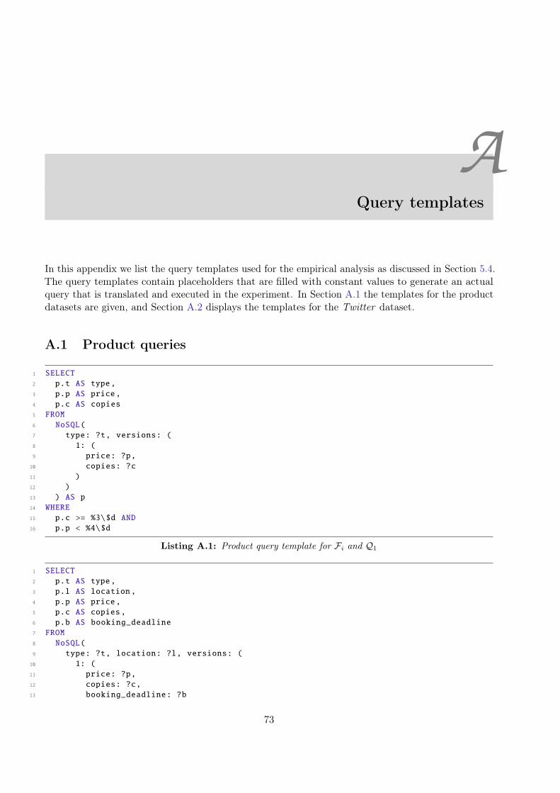
AQuery templates
In this appendix we list the query templates used for the empirical analysis as discussed in Section 5.4.The query templates contain placeholders that are filled with constant values to generate an actualquery that is translated and executed in the experiment. In Section A.1 the templates for the productdatasets are given, and Section A.2 displays the templates for the Twitter dataset.
A.1 Product queries
1 SELECT2 p.t AS type,3 p.p AS price,4 p.c AS copies5 FROM6 NoSQL(7 type: ?t, versions: (8 1: (9 price: ?p,10 copies: ?c11 )12 )13 ) AS p14 WHERE15 p.c >= %3\$d AND16 p.p < %4\$d
Listing A.1: Product query template for Fi and Q1
1 SELECT2 p.t AS type,3 p.l AS location,4 p.p AS price,5 p.c AS copies,6 p.b AS booking_deadline7 FROM8 NoSQL(9 type: ?t, location: ?l, versions: (10 1: (11 price: ?p,12 copies: ?c,13 booking_deadline: ?b
73
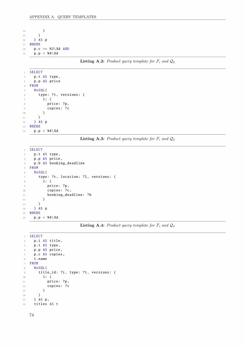
APPENDIX A. QUERY TEMPLATES
14 )15 )16 ) AS p17 WHERE18 p.c >= %3\$d AND19 p.p < %4\$d
Listing A.2: Product query template for Fi and Q2
1 SELECT2 p.t AS type,3 p.p AS price4 FROM5 NoSQL(6 type: ?t, versions: (7 1: (8 price: ?p,9 copies: ?c10 )11 )12 ) AS p13 WHERE14 p.p < %4\$d
Listing A.3: Product query template for Fi and Q3
1 SELECT2 p.t AS type,3 p.p AS price,4 p.b AS booking_deadline5 FROM6 NoSQL(7 type: ?t, location: ?l, versions: (8 1: (9 price: ?p,10 copies: ?c,11 booking_deadline: ?b12 )13 )14 ) AS p15 WHERE16 p.p < %4\$d
Listing A.4: Product query template for Fi and Q4
1 SELECT2 p.i AS title,3 p.t AS type,4 p.p AS price,5 p.c AS copies,6 t.name7 FROM8 NoSQL(9 title_id: ?i, type: ?t, versions: (10 1: (11 price: ?p,12 copies: ?c13 )14 )15 ) AS p,16 titles AS t
74
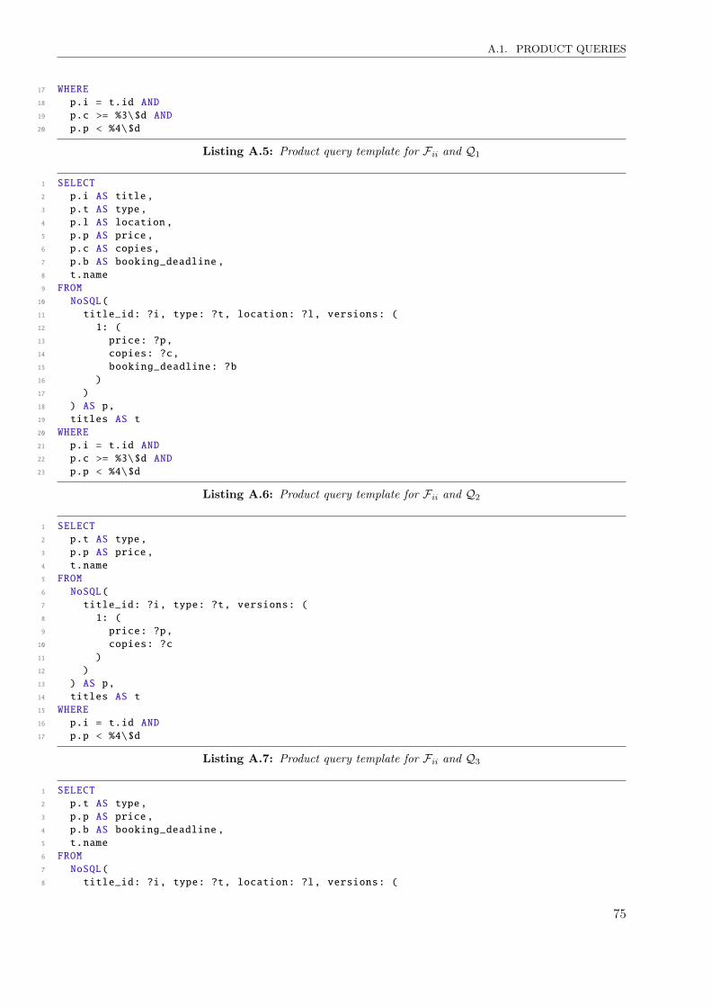
A.1. PRODUCT QUERIES
17 WHERE18 p.i = t.id AND19 p.c >= %3\$d AND20 p.p < %4\$d
Listing A.5: Product query template for Fii and Q1
1 SELECT2 p.i AS title,3 p.t AS type,4 p.l AS location,5 p.p AS price,6 p.c AS copies,7 p.b AS booking_deadline ,8 t.name9 FROM10 NoSQL(11 title_id: ?i, type: ?t, location: ?l, versions: (12 1: (13 price: ?p,14 copies: ?c,15 booking_deadline: ?b16 )17 )18 ) AS p,19 titles AS t20 WHERE21 p.i = t.id AND22 p.c >= %3\$d AND23 p.p < %4\$d
Listing A.6: Product query template for Fii and Q2
1 SELECT2 p.t AS type,3 p.p AS price,4 t.name5 FROM6 NoSQL(7 title_id: ?i, type: ?t, versions: (8 1: (9 price: ?p,10 copies: ?c11 )12 )13 ) AS p,14 titles AS t15 WHERE16 p.i = t.id AND17 p.p < %4\$d
Listing A.7: Product query template for Fii and Q3
1 SELECT2 p.t AS type,3 p.p AS price,4 p.b AS booking_deadline ,5 t.name6 FROM7 NoSQL(8 title_id: ?i, type: ?t, location: ?l, versions: (
75
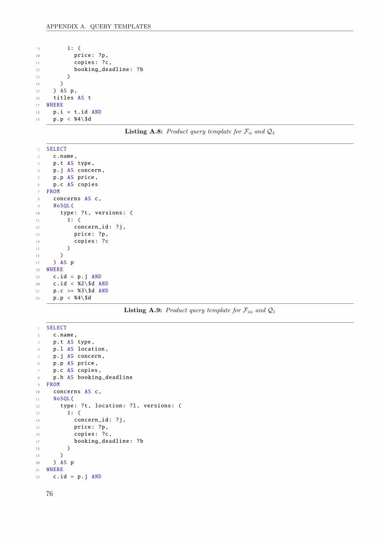
APPENDIX A. QUERY TEMPLATES
9 1: (10 price: ?p,11 copies: ?c,12 booking_deadline: ?b13 )14 )15 ) AS p,16 titles AS t17 WHERE18 p.i = t.id AND19 p.p < %4\$d
Listing A.8: Product query template for Fii and Q4
1 SELECT2 c.name,3 p.t AS type,4 p.j AS concern,5 p.p AS price,6 p.c AS copies7 FROM8 concerns AS c,9 NoSQL(10 type: ?t, versions: (11 1: (12 concern_id: ?j,13 price: ?p,14 copies: ?c15 )16 )17 ) AS p18 WHERE19 c.id = p.j AND20 c.id < %2\$d AND21 p.c >= %3\$d AND22 p.p < %4\$d
Listing A.9: Product query template for Fiii and Q1
1 SELECT2 c.name,3 p.t AS type,4 p.l AS location,5 p.j AS concern,6 p.p AS price,7 p.c AS copies,8 p.b AS booking_deadline9 FROM10 concerns AS c,11 NoSQL(12 type: ?t, location: ?l, versions: (13 1: (14 concern_id: ?j,15 price: ?p,16 copies: ?c,17 booking_deadline: ?b18 )19 )20 ) AS p21 WHERE22 c.id = p.j AND
76
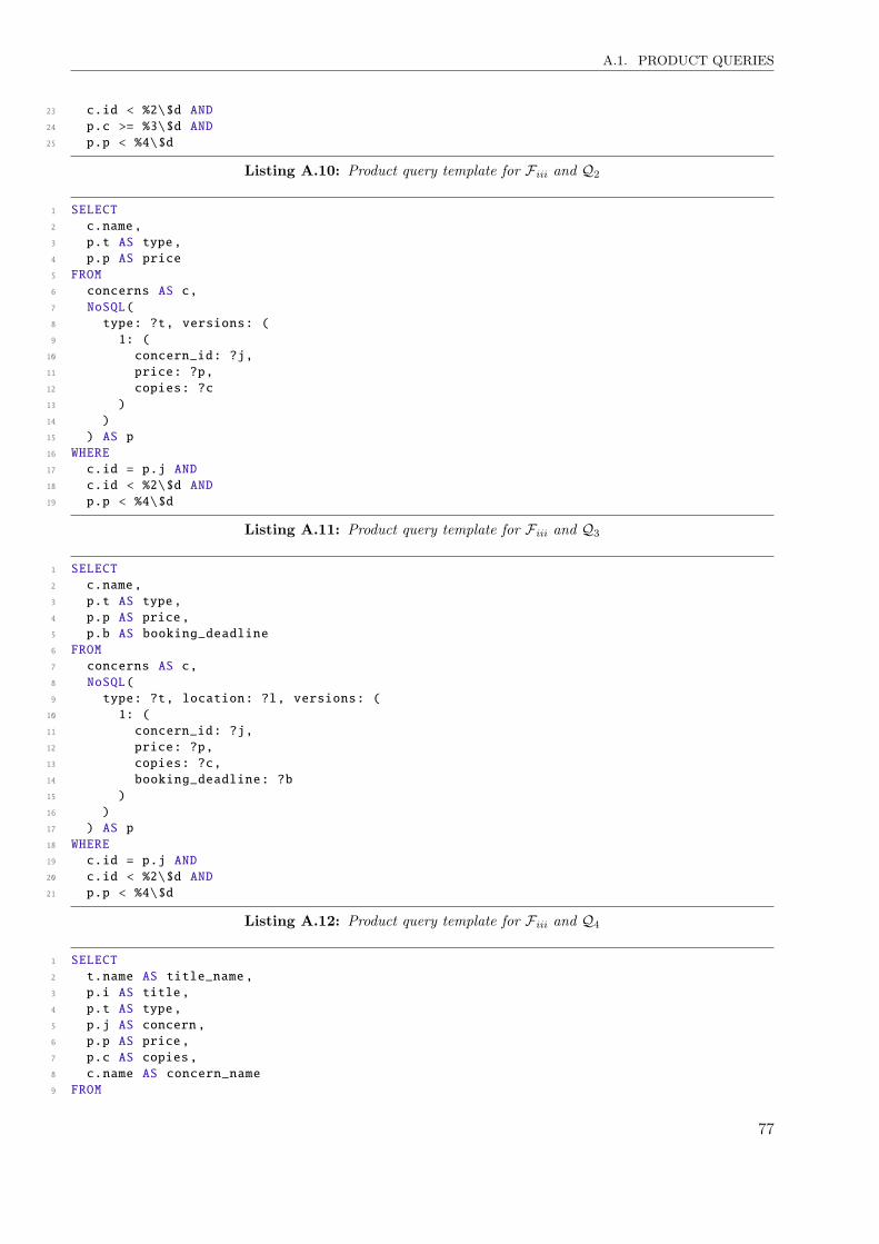
A.1. PRODUCT QUERIES
23 c.id < %2\$d AND24 p.c >= %3\$d AND25 p.p < %4\$d
Listing A.10: Product query template for Fiii and Q2
1 SELECT2 c.name,3 p.t AS type,4 p.p AS price5 FROM6 concerns AS c,7 NoSQL(8 type: ?t, versions: (9 1: (10 concern_id: ?j,11 price: ?p,12 copies: ?c13 )14 )15 ) AS p16 WHERE17 c.id = p.j AND18 c.id < %2\$d AND19 p.p < %4\$d
Listing A.11: Product query template for Fiii and Q3
1 SELECT2 c.name,3 p.t AS type,4 p.p AS price,5 p.b AS booking_deadline6 FROM7 concerns AS c,8 NoSQL(9 type: ?t, location: ?l, versions: (10 1: (11 concern_id: ?j,12 price: ?p,13 copies: ?c,14 booking_deadline: ?b15 )16 )17 ) AS p18 WHERE19 c.id = p.j AND20 c.id < %2\$d AND21 p.p < %4\$d
Listing A.12: Product query template for Fiii and Q4
1 SELECT2 t.name AS title_name ,3 p.i AS title,4 p.t AS type,5 p.j AS concern,6 p.p AS price,7 p.c AS copies,8 c.name AS concern_name9 FROM
77
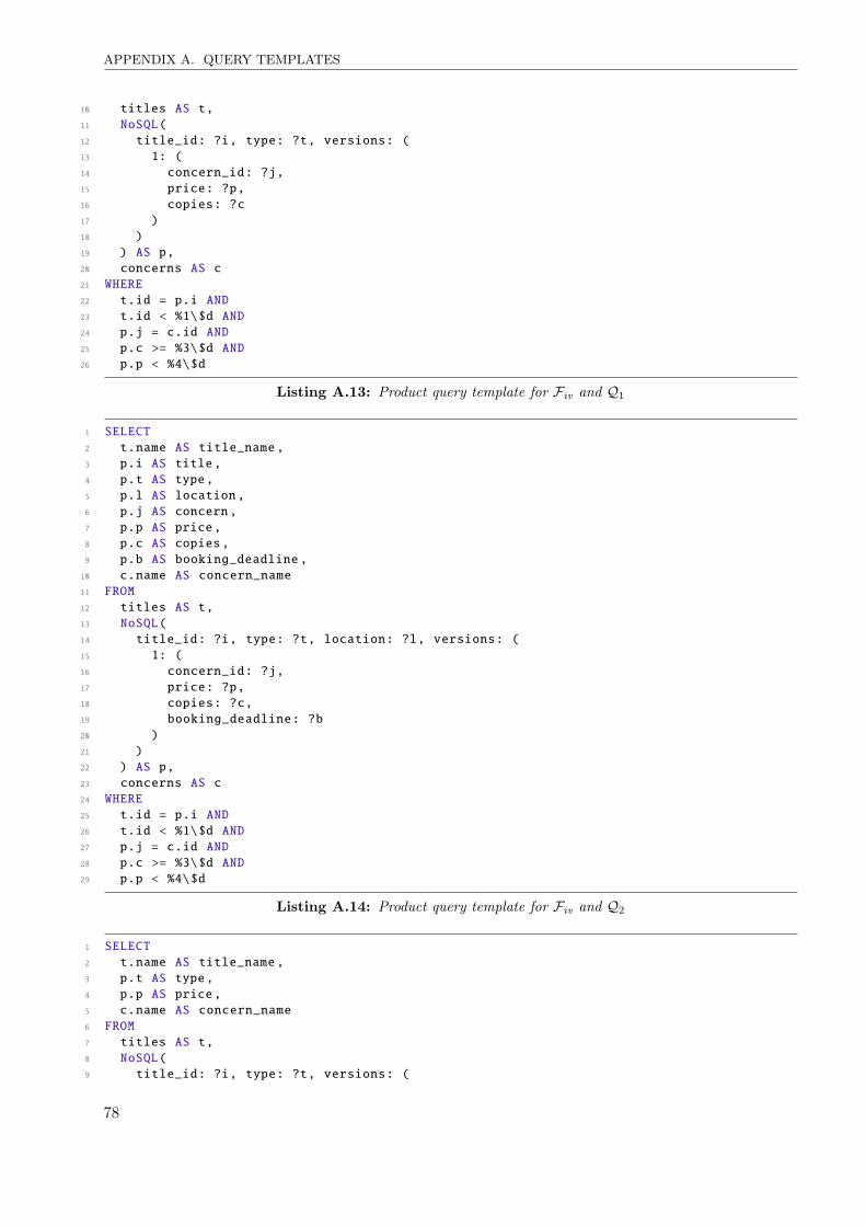
APPENDIX A. QUERY TEMPLATES
10 titles AS t,11 NoSQL(12 title_id: ?i, type: ?t, versions: (13 1: (14 concern_id: ?j,15 price: ?p,16 copies: ?c17 )18 )19 ) AS p,20 concerns AS c21 WHERE22 t.id = p.i AND23 t.id < %1\$d AND24 p.j = c.id AND25 p.c >= %3\$d AND26 p.p < %4\$d
Listing A.13: Product query template for Fiv and Q1
1 SELECT2 t.name AS title_name ,3 p.i AS title,4 p.t AS type,5 p.l AS location,6 p.j AS concern,7 p.p AS price,8 p.c AS copies,9 p.b AS booking_deadline ,10 c.name AS concern_name11 FROM12 titles AS t,13 NoSQL(14 title_id: ?i, type: ?t, location: ?l, versions: (15 1: (16 concern_id: ?j,17 price: ?p,18 copies: ?c,19 booking_deadline: ?b20 )21 )22 ) AS p,23 concerns AS c24 WHERE25 t.id = p.i AND26 t.id < %1\$d AND27 p.j = c.id AND28 p.c >= %3\$d AND29 p.p < %4\$d
Listing A.14: Product query template for Fiv and Q2
1 SELECT2 t.name AS title_name ,3 p.t AS type,4 p.p AS price,5 c.name AS concern_name6 FROM7 titles AS t,8 NoSQL(9 title_id: ?i, type: ?t, versions: (
78
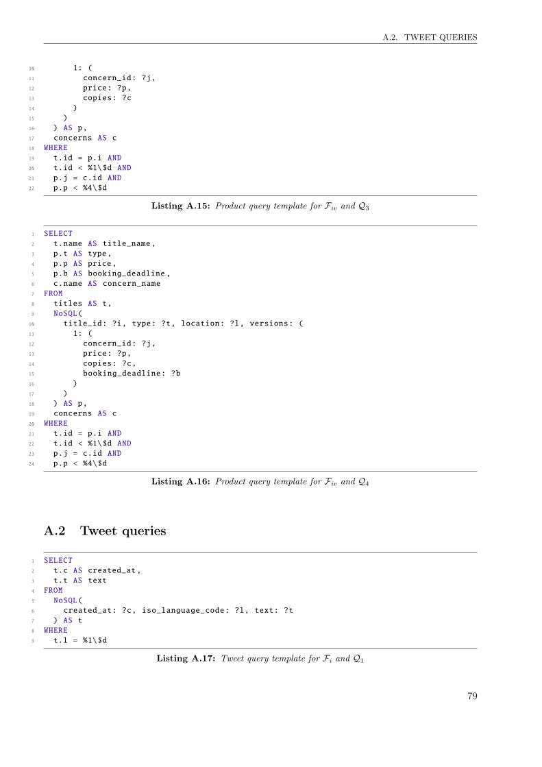
A.2. TWEET QUERIES
10 1: (11 concern_id: ?j,12 price: ?p,13 copies: ?c14 )15 )16 ) AS p,17 concerns AS c18 WHERE19 t.id = p.i AND20 t.id < %1\$d AND21 p.j = c.id AND22 p.p < %4\$d
Listing A.15: Product query template for Fiv and Q3
1 SELECT2 t.name AS title_name ,3 p.t AS type,4 p.p AS price,5 p.b AS booking_deadline ,6 c.name AS concern_name7 FROM8 titles AS t,9 NoSQL(10 title_id: ?i, type: ?t, location: ?l, versions: (11 1: (12 concern_id: ?j,13 price: ?p,14 copies: ?c,15 booking_deadline: ?b16 )17 )18 ) AS p,19 concerns AS c20 WHERE21 t.id = p.i AND22 t.id < %1\$d AND23 p.j = c.id AND24 p.p < %4\$d
Listing A.16: Product query template for Fiv and Q4
A.2 Tweet queries
1 SELECT2 t.c AS created_at ,3 t.t AS text4 FROM5 NoSQL(6 created_at: ?c, iso_language_code: ?l, text: ?t7 ) AS t8 WHERE9 t.l = %1\$d
Listing A.17: Tweet query template for Fi and Q1
79

APPENDIX A. QUERY TEMPLATES
1 SELECT2 t.c AS created_at ,3 t.t AS text,4 t.u AS url,5 t.m AS user_mention_id6 FROM7 NoSQL(8 created_at: ?c, iso_language_code: ?l, text: ?t, entities: (9 urls: (10 0: (11 url: ?u12 )13 ),14 user_mentions: (15 0: ?m16 )17 )18 ) AS t19 WHERE20 t.l = %1\$d
Listing A.18: Tweet query template for Fi and Q2
1 SELECT2 t.t AS text3 FROM4 NoSQL(5 created_at: ?c, iso_language_code: ?l, text: ?t6 ) AS t7 WHERE8 t.l = %1\$d
Listing A.19: Tweet query template for Fi and Q3
1 SELECT2 t.t AS text,3 t.m AS user_mention_id4 FROM5 NoSQL(6 created_at: ?c, iso_language_code: ?l, text: ?t, entities: (7 urls: (8 0: (9 url: ?u10 )11 ),12 user_mentions: (13 0: ?m14 )15 )16 ) AS t17 WHERE18 t.l = %1\$d
Listing A.20: Tweet query template for Fi and Q4
1 SELECT2 t.c AS created_at ,3 t.t AS text,4 u.name,5 u.screen_name
80
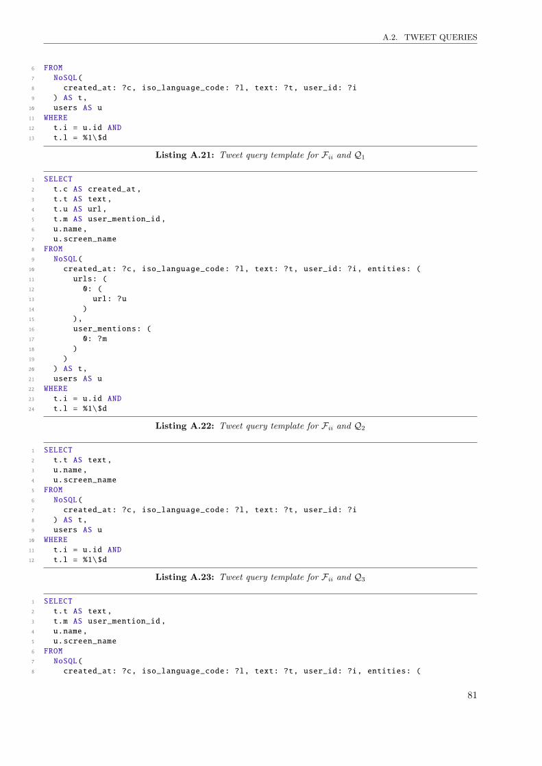
A.2. TWEET QUERIES
6 FROM7 NoSQL(8 created_at: ?c, iso_language_code: ?l, text: ?t, user_id: ?i9 ) AS t,10 users AS u11 WHERE12 t.i = u.id AND13 t.l = %1\$d
Listing A.21: Tweet query template for Fii and Q1
1 SELECT2 t.c AS created_at ,3 t.t AS text,4 t.u AS url,5 t.m AS user_mention_id ,6 u.name,7 u.screen_name8 FROM9 NoSQL(10 created_at: ?c, iso_language_code: ?l, text: ?t, user_id: ?i, entities: (11 urls: (12 0: (13 url: ?u14 )15 ),16 user_mentions: (17 0: ?m18 )19 )20 ) AS t,21 users AS u22 WHERE23 t.i = u.id AND24 t.l = %1\$d
Listing A.22: Tweet query template for Fii and Q2
1 SELECT2 t.t AS text,3 u.name,4 u.screen_name5 FROM6 NoSQL(7 created_at: ?c, iso_language_code: ?l, text: ?t, user_id: ?i8 ) AS t,9 users AS u10 WHERE11 t.i = u.id AND12 t.l = %1\$d
Listing A.23: Tweet query template for Fii and Q3
1 SELECT2 t.t AS text,3 t.m AS user_mention_id ,4 u.name,5 u.screen_name6 FROM7 NoSQL(8 created_at: ?c, iso_language_code: ?l, text: ?t, user_id: ?i, entities: (
81
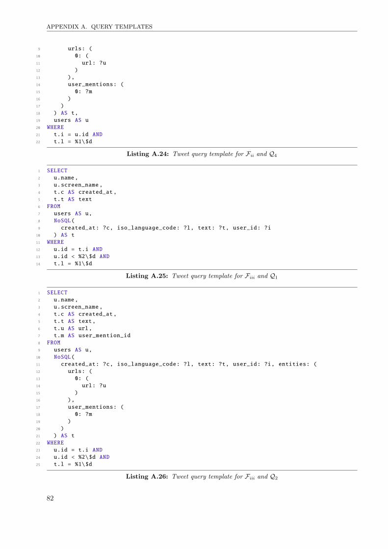
APPENDIX A. QUERY TEMPLATES
9 urls: (10 0: (11 url: ?u12 )13 ),14 user_mentions: (15 0: ?m16 )17 )18 ) AS t,19 users AS u20 WHERE21 t.i = u.id AND22 t.l = %1\$d
Listing A.24: Tweet query template for Fii and Q4
1 SELECT2 u.name,3 u.screen_name ,4 t.c AS created_at ,5 t.t AS text6 FROM7 users AS u,8 NoSQL(9 created_at: ?c, iso_language_code: ?l, text: ?t, user_id: ?i10 ) AS t11 WHERE12 u.id = t.i AND13 u.id < %2\$d AND14 t.l = %1\$d
Listing A.25: Tweet query template for Fiii and Q1
1 SELECT2 u.name,3 u.screen_name ,4 t.c AS created_at ,5 t.t AS text,6 t.u AS url,7 t.m AS user_mention_id8 FROM9 users AS u,10 NoSQL(11 created_at: ?c, iso_language_code: ?l, text: ?t, user_id: ?i, entities: (12 urls: (13 0: (14 url: ?u15 )16 ),17 user_mentions: (18 0: ?m19 )20 )21 ) AS t22 WHERE23 u.id = t.i AND24 u.id < %2\$d AND25 t.l = %1\$d
Listing A.26: Tweet query template for Fiii and Q2
82
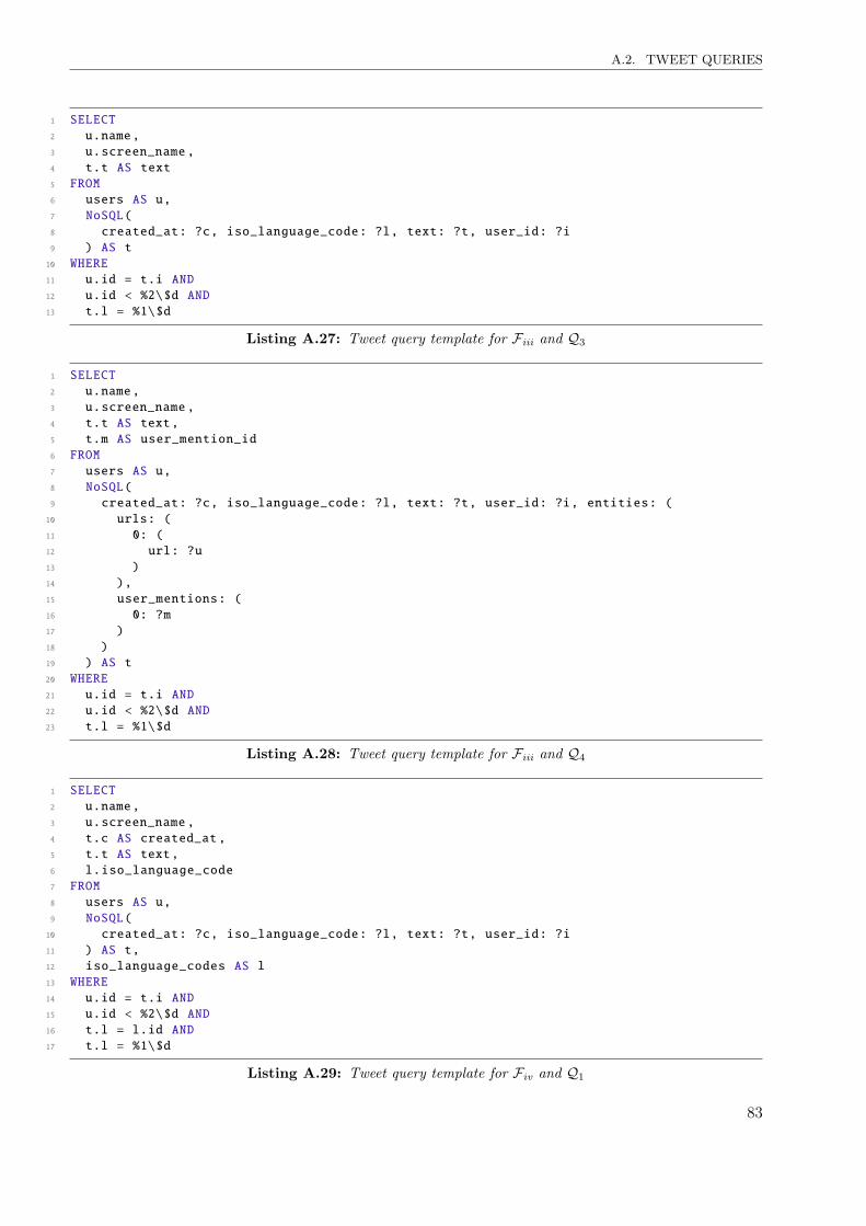
A.2. TWEET QUERIES
1 SELECT2 u.name,3 u.screen_name ,4 t.t AS text5 FROM6 users AS u,7 NoSQL(8 created_at: ?c, iso_language_code: ?l, text: ?t, user_id: ?i9 ) AS t10 WHERE11 u.id = t.i AND12 u.id < %2\$d AND13 t.l = %1\$d
Listing A.27: Tweet query template for Fiii and Q3
1 SELECT2 u.name,3 u.screen_name ,4 t.t AS text,5 t.m AS user_mention_id6 FROM7 users AS u,8 NoSQL(9 created_at: ?c, iso_language_code: ?l, text: ?t, user_id: ?i, entities: (10 urls: (11 0: (12 url: ?u13 )14 ),15 user_mentions: (16 0: ?m17 )18 )19 ) AS t20 WHERE21 u.id = t.i AND22 u.id < %2\$d AND23 t.l = %1\$d
Listing A.28: Tweet query template for Fiii and Q4
1 SELECT2 u.name,3 u.screen_name ,4 t.c AS created_at ,5 t.t AS text,6 l.iso_language_code7 FROM8 users AS u,9 NoSQL(10 created_at: ?c, iso_language_code: ?l, text: ?t, user_id: ?i11 ) AS t,12 iso_language_codes AS l13 WHERE14 u.id = t.i AND15 u.id < %2\$d AND16 t.l = l.id AND17 t.l = %1\$d
Listing A.29: Tweet query template for Fiv and Q1
83
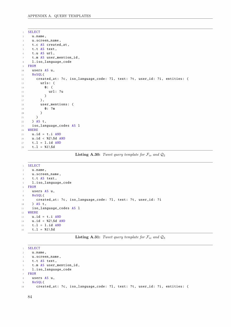
APPENDIX A. QUERY TEMPLATES
1 SELECT2 u.name,3 u.screen_name ,4 t.c AS created_at ,5 t.t AS text,6 t.u AS url,7 t.m AS user_mention_id ,8 l.iso_language_code9 FROM10 users AS u,11 NoSQL(12 created_at: ?c, iso_language_code: ?l, text: ?t, user_id: ?i, entities: (13 urls: (14 0: (15 url: ?u16 )17 ),18 user_mentions: (19 0: ?m20 )21 )22 ) AS t,23 iso_language_codes AS l24 WHERE25 u.id = t.i AND26 u.id < %2\$d AND27 t.l = l.id AND28 t.l = %1\$d
Listing A.30: Tweet query template for Fiv and Q2
1 SELECT2 u.name,3 u.screen_name ,4 t.t AS text,5 l.iso_language_code6 FROM7 users AS u,8 NoSQL(9 created_at: ?c, iso_language_code: ?l, text: ?t, user_id: ?i10 ) AS t,11 iso_language_codes AS l12 WHERE13 u.id = t.i AND14 u.id < %2\$d AND15 t.l = l.id AND16 t.l = %1\$d
Listing A.31: Tweet query template for Fiv and Q3
1 SELECT2 u.name,3 u.screen_name ,4 t.t AS text,5 t.m AS user_mention_id ,6 l.iso_language_code7 FROM8 users AS u,9 NoSQL(10 created_at: ?c, iso_language_code: ?l, text: ?t, user_id: ?i, entities: (
84
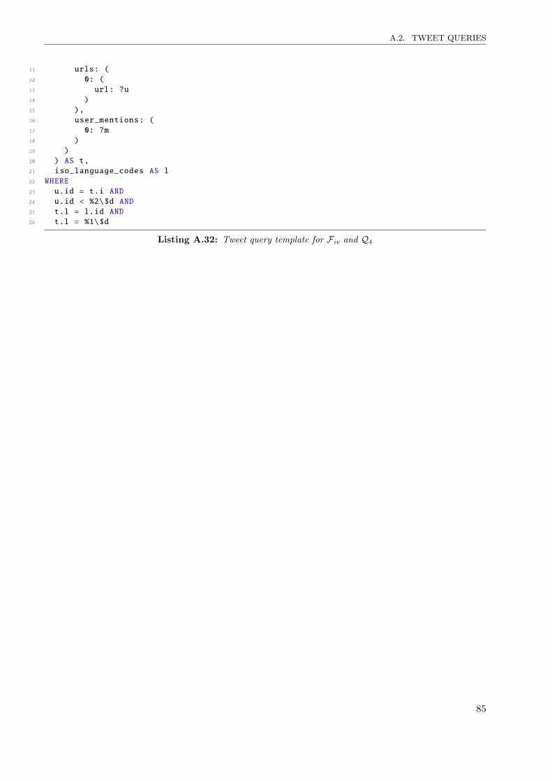
A.2. TWEET QUERIES
11 urls: (12 0: (13 url: ?u14 )15 ),16 user_mentions: (17 0: ?m18 )19 )20 ) AS t,21 iso_language_codes AS l22 WHERE23 u.id = t.i AND24 u.id < %2\$d AND25 t.l = l.id AND26 t.l = %1\$d
Listing A.32: Tweet query template for Fiv and Q4
85

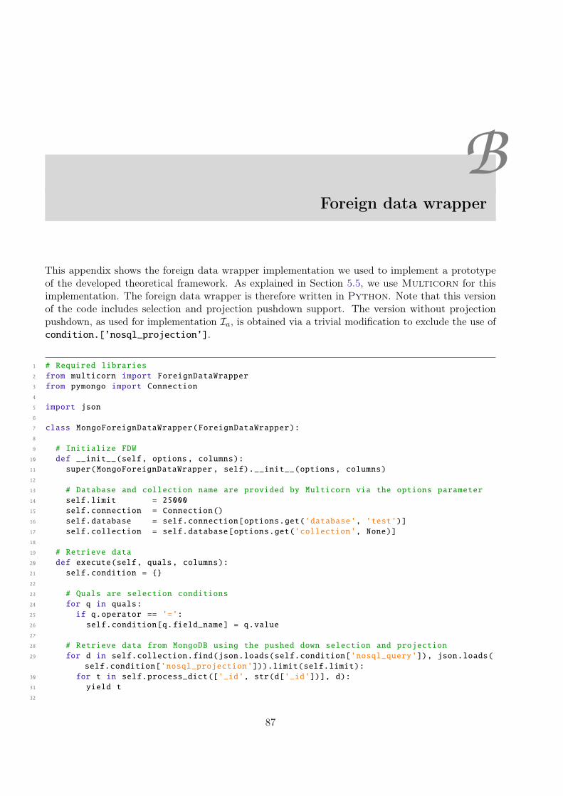
BForeign data wrapper
This appendix shows the foreign data wrapper implementation we used to implement a prototypeof the developed theoretical framework. As explained in Section 5.5, we use Multicorn for thisimplementation. The foreign data wrapper is therefore written in Python. Note that this versionof the code includes selection and projection pushdown support. The version without projectionpushdown, as used for implementation Ia, is obtained via a trivial modification to exclude the use ofcondition.[’nosql_projection’].
1 # Required libraries2 from multicorn import ForeignDataWrapper3 from pymongo import Connection4
5 import json6
7 class MongoForeignDataWrapper(ForeignDataWrapper):8
9 # Initialize FDW10 def __init__(self, options, columns):11 super(MongoForeignDataWrapper , self).__init__(options, columns)12
13 # Database and collection name are provided by Multicorn via the options parameter14 self.limit = 2500015 self.connection = Connection()16 self.database = self.connection[options.get('database', 'test')]17 self.collection = self.database[options.get('collection', None)]18
19 # Retrieve data20 def execute(self, quals, columns):21 self.condition = {}22
23 # Quals are selection conditions24 for q in quals:25 if q.operator == '=':26 self.condition[q.field_name] = q.value27
28 # Retrieve data from MongoDB using the pushed down selection and projection29 for d in self.collection.find(json.loads(self.condition['nosql_query']), json.loads(
self.condition['nosql_projection'])).limit(self.limit):30 for t in self.process_dict(['_id', str(d['_id'])], d):31 yield t32
87
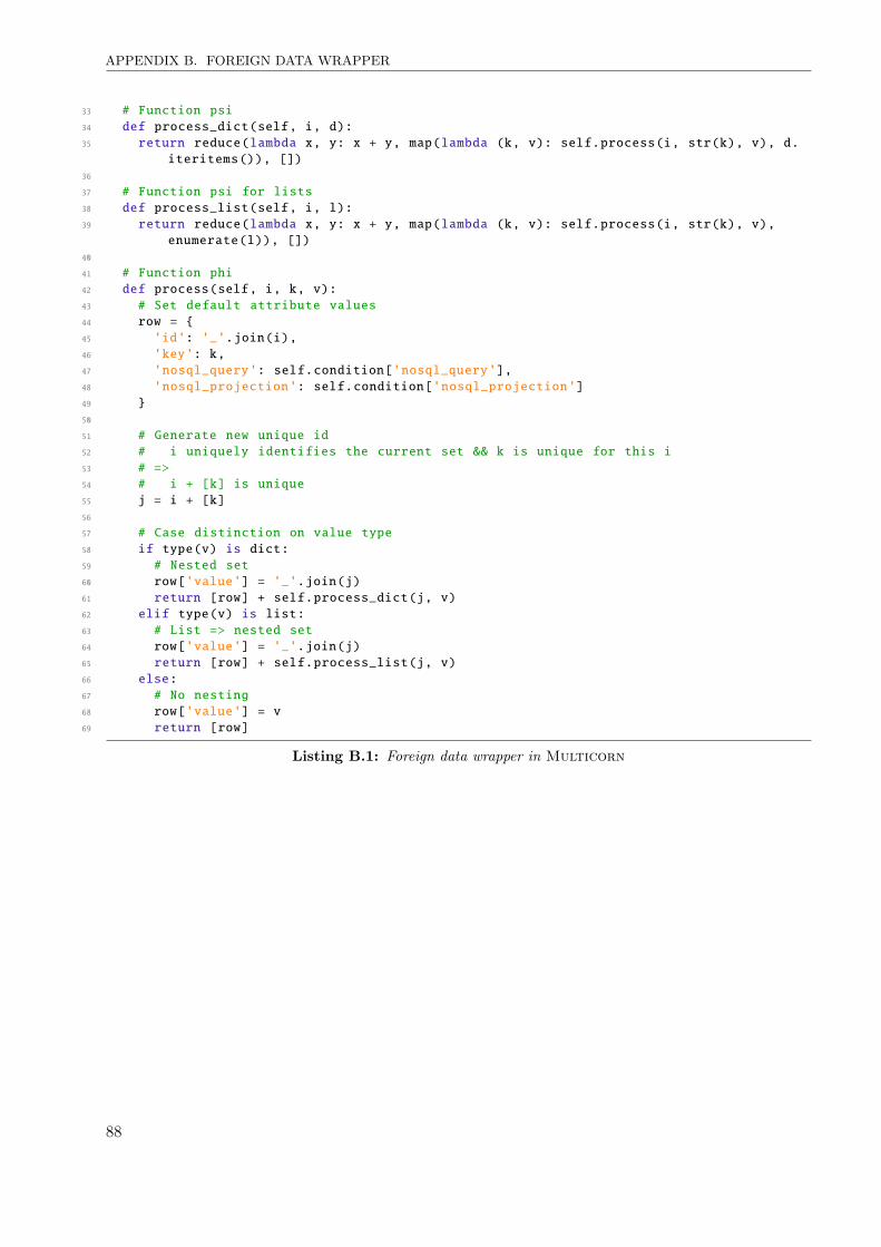
APPENDIX B. FOREIGN DATA WRAPPER
33 # Function psi34 def process_dict(self, i, d):35 return reduce(lambda x, y: x + y, map(lambda (k, v): self.process(i, str(k), v), d.
iteritems()), [])36
37 # Function psi for lists38 def process_list(self, i, l):39 return reduce(lambda x, y: x + y, map(lambda (k, v): self.process(i, str(k), v),
enumerate(l)), [])40
41 # Function phi42 def process(self, i, k, v):43 # Set default attribute values44 row = {45 'id': '_'.join(i),46 'key': k,47 'nosql_query': self.condition['nosql_query'],48 'nosql_projection': self.condition['nosql_projection']49 }50
51 # Generate new unique id52 # i uniquely identifies the current set && k is unique for this i53 # =>54 # i + [k] is unique55 j = i + [k]56
57 # Case distinction on value type58 if type(v) is dict:59 # Nested set60 row['value'] = '_'.join(j)61 return [row] + self.process_dict(j, v)62 elif type(v) is list:63 # List => nested set64 row['value'] = '_'.join(j)65 return [row] + self.process_list(j, v)66 else:67 # No nesting68 row['value'] = v69 return [row]
Listing B.1: Foreign data wrapper in Multicorn
88
Bibliography
[ASX01] Rakesh Agrawal, Amit Somani, and Yirong Xu. Storage and querying of e-commerce data.In Proceedings of the 27th VLDB Conference, VLDB ’01. VLDB Endowment, 2001.
[Cat10] Rick Cattell. Scalable SQL and NoSQL data stores. SIGMOD Record, 39(4):12–27,December 2010.
[CDES05] Eugene Inseok Chong, Souripriya Das, George Eadon, and Jagannathan Srinivasan. Anefficient SQL-based RDF querying scheme. In Proceedings of the 31st VLDB Conference,VLDB ’05, pages 1216–1227. VLDB Endowment, 2005.
[CLF09] Artem Chebotko, Shiyong Lu, and Farshad Fotouhi. Semantics preserving SPARQL-to-SQLtranslation. Data & Knowledge Engineering, 68(10):973–1000, 2009.
[DS09] Souripriya Das and Jagannathan Srinivasan. Database technologies for RDF. In ReasoningWeb, volume 5689 of Lecture Notes in Computer Science, pages 205–221. Springer-VerlagBerlin Heidelberg, 2009.
[FB09] George H.L. Fletcher and Peter W. Beck. Scalable indexing of RDF graphs for efficientjoin processing. In Proceeding of the 18th ACM conference on Information and knowledgemanagement, CIKM ’09, pages 1513–1516, Hong Kong, China, November 2009. ACM.
[FW09] George H.L. Fletcher and Catharine M. Wyss. Towards a general framework for effectivesolutions to the data mapping problem. In Journal on Data Semantics XIV, volume 5880 ofLecture Notes in Computer Science, pages 37–73. Springer-Verlag Berlin Heidelberg, 2009.
[GC07] Gang Gou and Rada Chirkova. Efficiently querying large XML data repositories: A survey.IEEE Transactions on Knowledge and Data Engineering, 19(10):1381 –1403, October 2007.
[LKK91] Witold Litwin, M. Ketabchi, and Ravi Krishnamurthy. First order normal form for relationaldatabases and multidatabases. SIGMOD Record, 20(4):74–76, December 1991.
[Sto10] Michael Stonebraker. SQL databases v. NoSQL databases. Communications of the ACM,53(4):10–11, April 2010.
[Var09] Ian Thomas Varley. No relation: The mixed blessings of non-relational databases. Master’sthesis, The University of Texas at Austin, August 2009.
89

BIBLIOGRAPHY
[Wie92] Gio Wiederhold. Mediators in the architecture of future information systems. Computer,25(3):38–49, March 1992.
90