Embed Size (px)
Citation preview

Bridging the two cultures: Latent
variable statistical modeling with
boosted regression trees
Thomas G. Dietterich and Rebecca Hutchinson
11/15/2012 ESA 2012 1
Oregon State University
Corvallis, Oregon, USA
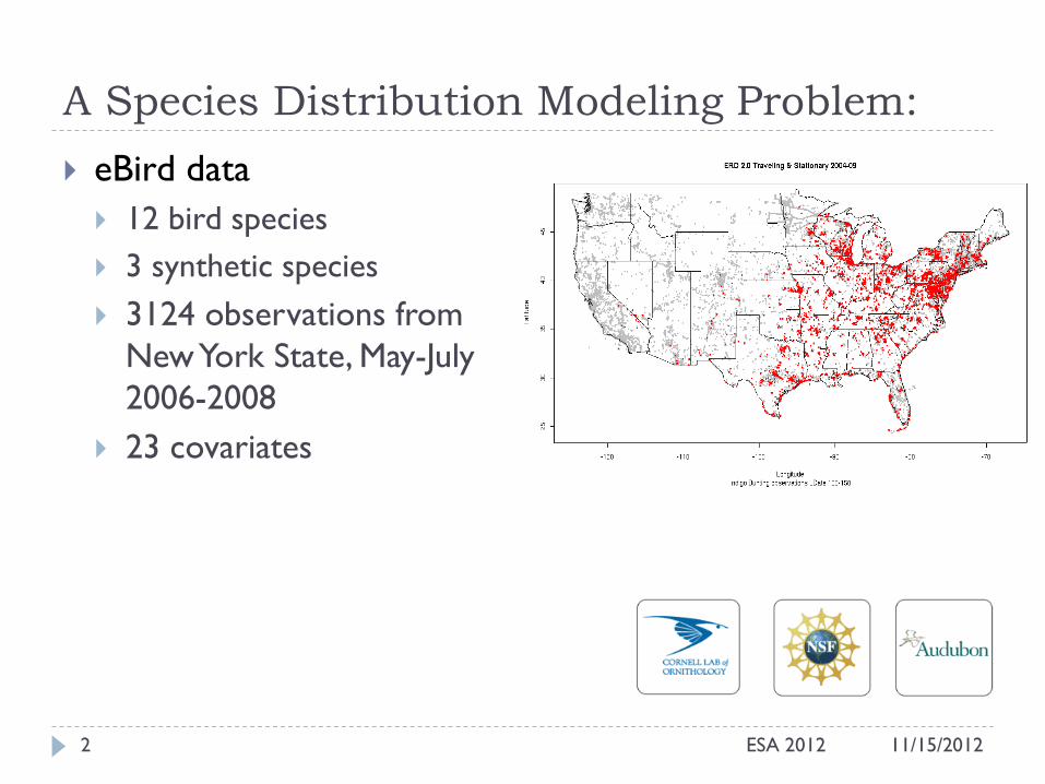
A Species Distribution Modeling Problem:
11/15/2012 ESA 2012 2
eBird data
12 bird species
3 synthetic species
3124 observations from
New York State, May-July
2006-2008
23 covariates
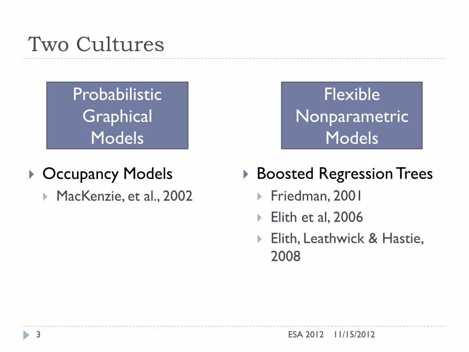
Two Cultures
11/15/2012 ESA 2012 3
Occupancy Models
MacKenzie, et al., 2002
Boosted Regression Trees
Friedman, 2001
Elith et al, 2006
Elith, Leathwick & Hastie,
2008
Probabilistic
Graphical
Models
Flexible
Nonparametric
Models
4
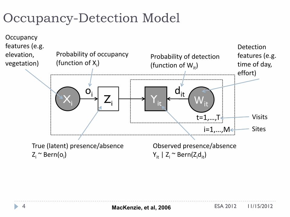
Occupancy-Detection Model
Yit Zi
i=1,…,M
t=1,…,T
Xi Wit
oi dit
Occupancy features (e.g. elevation, vegetation)
Detection features (e.g. time of day, effort)
Observed presence/absence Yit | Zi ~ Bern(Zidit)
True (latent) presence/absence Zi ~ Bern(oi)
Probability of occupancy (function of Xi)
Probability of detection (function of Wit)
Sites
Visits
MacKenzie, et al, 2006
11/15/2012 ESA 2012
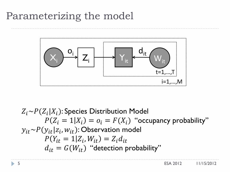
Parameterizing the model
Yit Zi
i=1,…,M
t=1,…,T
Xi Wit
oi dit
𝑍𝑖~𝑃(𝑍𝑖|𝑋𝑖): Species Distribution Model
𝑃 𝑍𝑖 = 1 𝑋𝑖 = 𝑜𝑖 = 𝐹(𝑋𝑖) “occupancy probability”
𝑦𝑖𝑡~𝑃(𝑦𝑖𝑡|𝑧𝑖 , 𝑤𝑖𝑡): Observation model
𝑃 𝑌𝑖𝑡 = 1 𝑍𝑖 , 𝑊𝑖𝑡 = 𝑍𝑖𝑑𝑖𝑡
𝑑𝑖𝑡 = 𝐺(𝑊𝑖𝑡) “detection probability”
11/15/2012 ESA 2012 5
Standard Approach: Log Linear (logistic
regression) models
11/15/2012 ESA 2012 6
log𝐹 𝑋𝑖
1−𝐹 𝑋𝑖= 𝛽0 + 𝛽1𝑋𝑖1 + ⋯ + 𝛽𝐽𝑋𝑖𝐽
log𝐺 𝑊𝑖𝑡
1−𝐺 𝑊𝑖𝑡= 𝛼0 + 𝛼1𝑊𝑖𝑡1 + ⋯ + 𝛼𝐾𝑊𝑖𝑡𝐾
Fit via maximum likelihood
Can apply hypothesis tests to assess importance of
covariates
𝐻0: 𝛽1 = 0
𝐻𝑎: 𝛽1 > 0
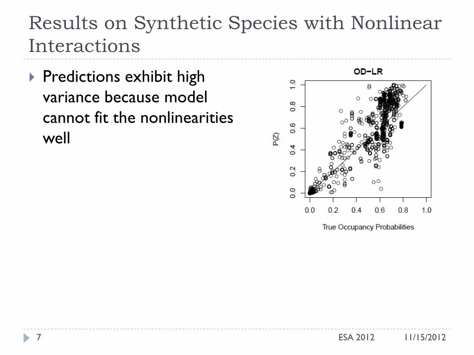
Results on Synthetic Species with Nonlinear
Interactions
11/15/2012 ESA 2012 7
Predictions exhibit high
variance because model
cannot fit the nonlinearities
well
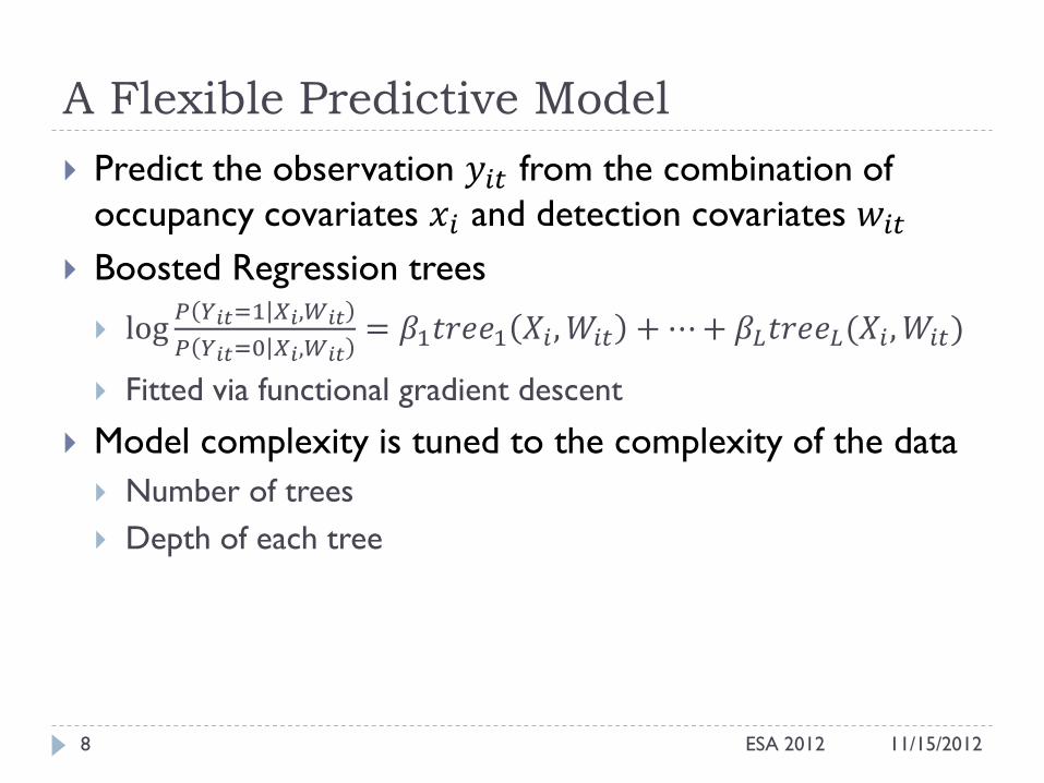
A Flexible Predictive Model
11/15/2012 ESA 2012 8
Predict the observation 𝑦𝑖𝑡 from the combination of
occupancy covariates 𝑥𝑖 and detection covariates 𝑤𝑖𝑡
Boosted Regression trees
log𝑃 𝑌𝑖𝑡=1 𝑋𝑖,𝑊𝑖𝑡
𝑃 𝑌𝑖𝑡=0 𝑋𝑖,𝑊𝑖𝑡= 𝛽1𝑡𝑟𝑒𝑒1 𝑋𝑖 , 𝑊𝑖𝑡 + ⋯ + 𝛽𝐿𝑡𝑟𝑒𝑒𝐿(𝑋𝑖 , 𝑊𝑖𝑡)
Fitted via functional gradient descent
Model complexity is tuned to the complexity of the data
Number of trees
Depth of each tree
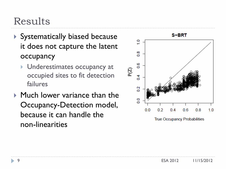
Results
11/15/2012 ESA 2012 9
Systematically biased because
it does not capture the latent
occupancy
Underestimates occupancy at
occupied sites to fit detection
failures
Much lower variance than the
Occupancy-Detection model,
because it can handle the
non-linearities P(Z
)
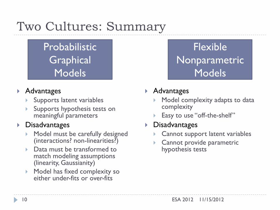
Two Cultures: Summary
11/15/2012 ESA 2012 10
Advantages Supports latent variables
Supports hypothesis tests on meaningful parameters
Disadvantages Model must be carefully designed
(interactions? non-linearities?)
Data must be transformed to match modeling assumptions (linearity, Gaussianity)
Model has fixed complexity so either under-fits or over-fits
Advantages Model complexity adapts to data
complexity
Easy to use “off-the-shelf”
Disadvantages Cannot support latent variables
Cannot provide parametric hypothesis tests
Probabilistic
Graphical
Models
Flexible
Nonparametric
Models
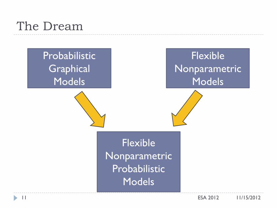
The Dream
Probabilistic
Graphical
Models
Flexible
Nonparametric
Models
Flexible
Nonparametric
Probabilistic
Models
11/15/2012 ESA 2012 11
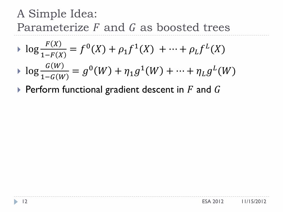
A Simple Idea:
Parameterize 𝐹 and 𝐺 as boosted trees
11/15/2012 ESA 2012 12
log𝐹 𝑋
1−𝐹 𝑋= 𝑓0(𝑋) + 𝜌1𝑓1(𝑋) + ⋯ + 𝜌𝐿𝑓𝐿(𝑋)
log𝐺 𝑊
1−𝐺 𝑊= 𝑔0 𝑊 + 𝜂1𝑔1 𝑊 + ⋯ + 𝜂𝐿𝑔
𝐿(𝑊)
Perform functional gradient descent in 𝐹 and 𝐺
11/15/2012 ESA 2012 13
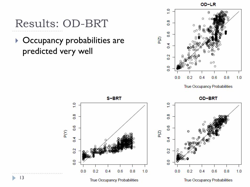
Results: OD-BRT
Occupancy probabilities are
predicted very well
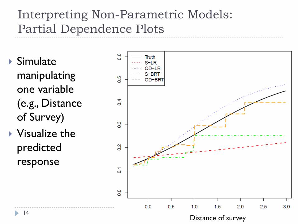
Interpreting Non-Parametric Models:
Partial Dependence Plots
11/15/2012 ESA 2012 14
Simulate
manipulating
one variable
(e.g., Distance
of Survey)
Visualize the
predicted
response
Distance of survey
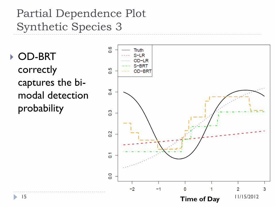
Partial Dependence Plot
Synthetic Species 3
OD-BRT
correctly
captures the bi-
modal detection
probability
11/15/2012 ESA 2012 15 Time of Day
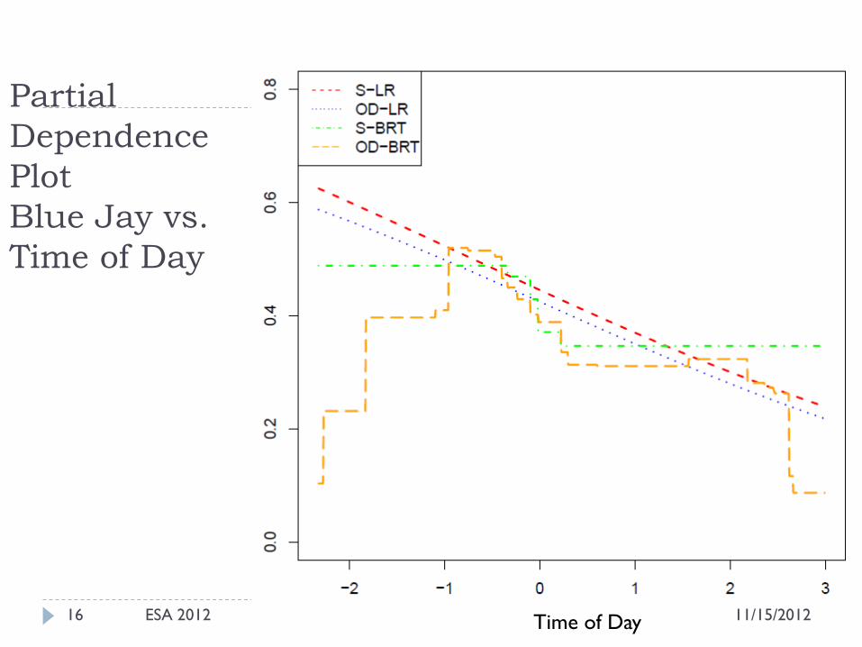
Partial
Dependence
Plot
Blue Jay vs.
Time of Day
11/15/2012 ESA 2012 16 Time of Day
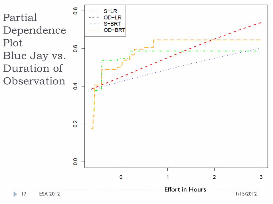
Partial
Dependence
Plot
Blue Jay vs.
Duration of
Observation
11/15/2012 ESA 2012 17 Effort in Hours
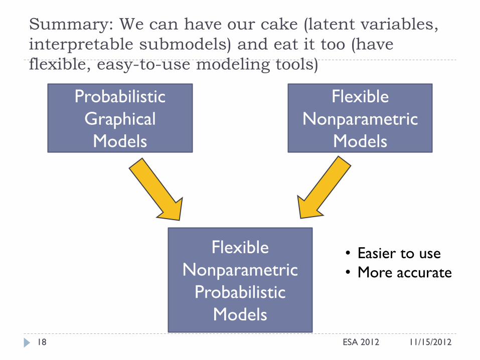
Summary: We can have our cake (latent variables,
interpretable submodels) and eat it too (have
flexible, easy-to-use modeling tools)
Probabilistic
Graphical
Models
Flexible
Nonparametric
Models
Flexible
Nonparametric
Probabilistic
Models
11/15/2012 ESA 2012 18
• Easier to use
• More accurate
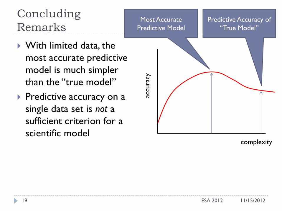
Concluding
Remarks
11/15/2012 ESA 2012 19
With limited data, the
most accurate predictive
model is much simpler
than the “true model”
Predictive accuracy on a
single data set is not a
sufficient criterion for a
scientific model
complexity
accu
racy
Most Accurate
Predictive Model
Predictive Accuracy of
“True Model”
Acknowledgements
11/15/2012 ESA 2012 20
Liping Liu: Boosted Regression Trees in OD models
Steve Kelling and colleagues at the Cornell Lab of
Ornithology
National Science Foundation Grants 0083292, 0307592,
0832804, and 0905885

11/15/2012 ESA 2012 21

11/15/2012 ESA 2012 22
Supporting Materials
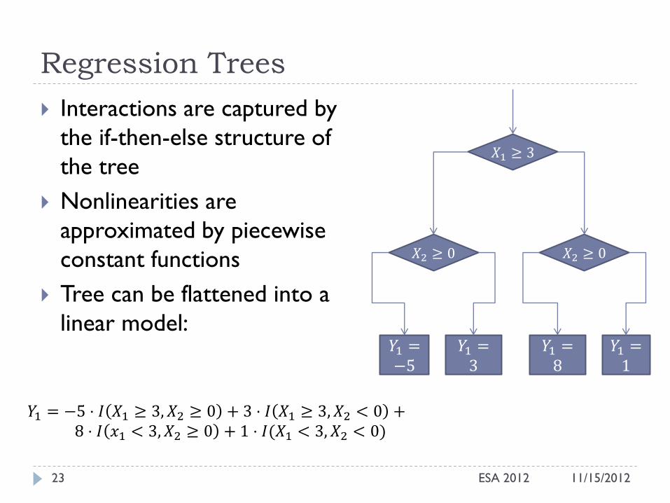
Regression Trees
11/15/2012 ESA 2012 23
Interactions are captured by
the if-then-else structure of
the tree
Nonlinearities are
approximated by piecewise
constant functions
Tree can be flattened into a
linear model:
𝑋1 ≥ 3
𝑋2 ≥ 0 𝑋2 ≥ 0
𝑌1 = −5
𝑌1 = 3
𝑌1 = 8
𝑌1 = 1
𝑌1 = −5 ⋅ 𝐼 𝑋1 ≥ 3, 𝑋2 ≥ 0 + 3 ⋅ 𝐼 𝑋1 ≥ 3, 𝑋2 < 0 + 8 ⋅ 𝐼 𝑥1 < 3, 𝑋2 ≥ 0 + 1 ⋅ 𝐼(𝑋1 < 3, 𝑋2 < 0)
Functional Gradient Descent
Boosted Regression Trees
11/15/2012 ESA 2012 24
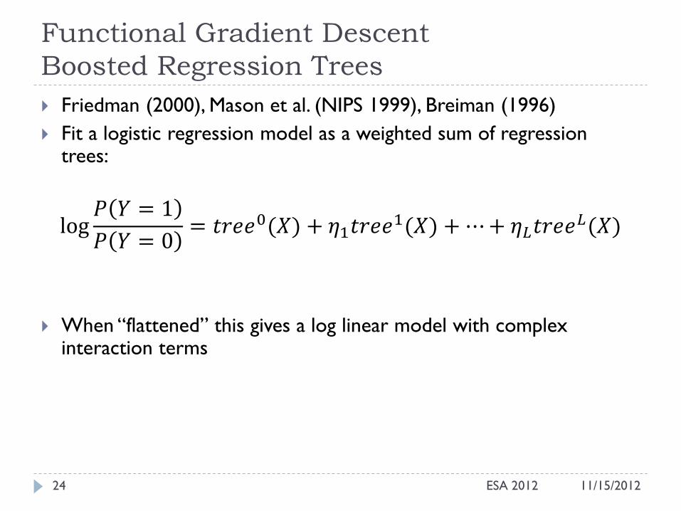
Friedman (2000), Mason et al. (NIPS 1999), Breiman (1996)
Fit a logistic regression model as a weighted sum of regression trees:
log𝑃 𝑌 = 1
𝑃 𝑌 = 0= 𝑡𝑟𝑒𝑒0(𝑋) + 𝜂1𝑡𝑟𝑒𝑒1(𝑋) + ⋯ + 𝜂𝐿𝑡𝑟𝑒𝑒𝐿(𝑋)
When “flattened” this gives a log linear model with complex interaction terms
L2-Tree Boosting Algorithm
11/15/2012 ESA 2012 25
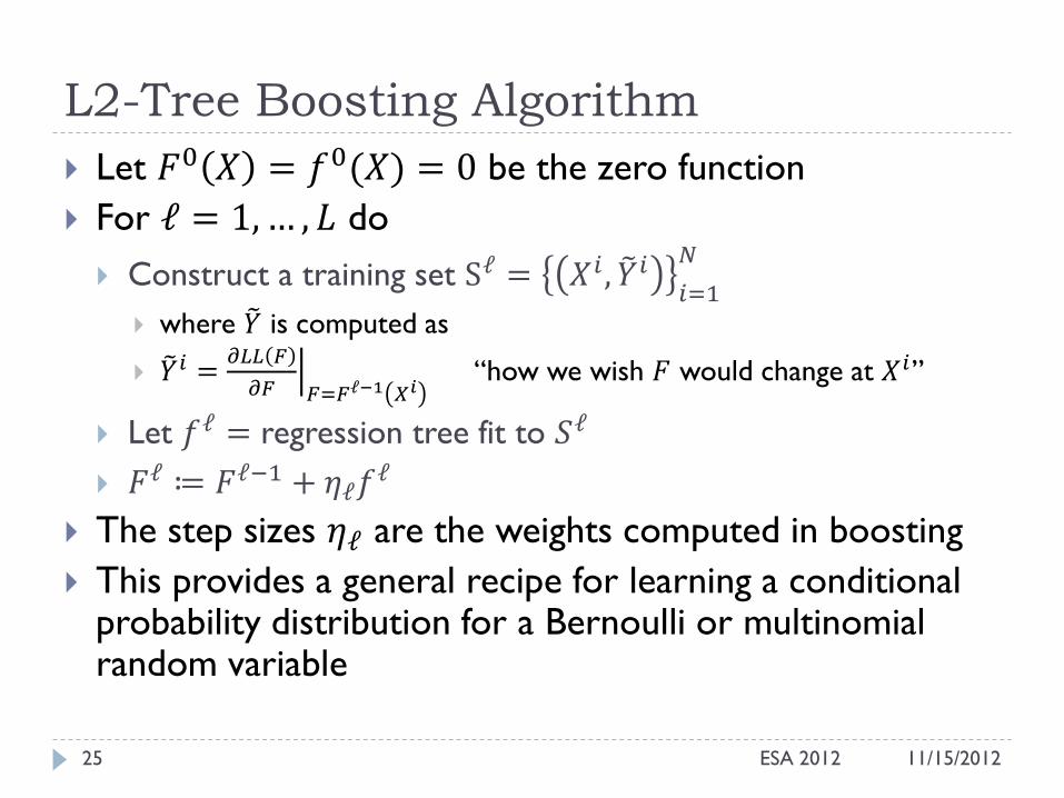
Let 𝐹0 𝑋 = 𝑓0(𝑋) = 0 be the zero function
For ℓ = 1, … , 𝐿 do
Construct a training set Sℓ = 𝑋𝑖 , 𝑌 𝑖𝑖=1
𝑁
where 𝑌 is computed as
𝑌 𝑖 =𝜕𝐿𝐿 𝐹
𝜕𝐹 𝐹=𝐹ℓ−1 𝑋𝑖
“how we wish 𝐹 would change at 𝑋𝑖”
Let 𝑓ℓ = regression tree fit to 𝑆ℓ
𝐹ℓ ≔ 𝐹ℓ−1 + 𝜂ℓ𝑓ℓ
The step sizes 𝜂ℓ are the weights computed in boosting
This provides a general recipe for learning a conditional probability distribution for a Bernoulli or multinomial random variable
Alternating Functional Gradient Descent
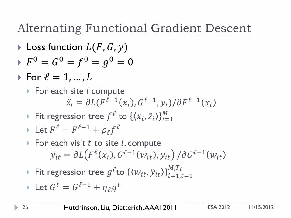
Loss function 𝐿(𝐹, 𝐺, 𝑦)
𝐹0 = 𝐺0 = 𝑓0 = 𝑔0 = 0
For ℓ = 1, … , 𝐿
For each site 𝑖 compute
𝑧 𝑖 = 𝜕𝐿(𝐹ℓ−1 𝑥𝑖 , 𝐺ℓ−1, 𝑦𝑖)/𝜕𝐹ℓ−1 𝑥𝑖
Fit regression tree 𝑓ℓ to 𝑥𝑖 , 𝑧 𝑖 𝑖=1𝑀
Let 𝐹ℓ = 𝐹ℓ−1 + 𝜌ℓ𝑓ℓ
For each visit 𝑡 to site 𝑖, compute
𝑦 𝑖𝑡 = 𝜕𝐿 𝐹ℓ 𝑥𝑖 , 𝐺ℓ−1 𝑤𝑖𝑡 , 𝑦𝑖𝑡 /𝜕𝐺ℓ−1 𝑤𝑖𝑡
Fit regression tree 𝑔ℓto 𝑤𝑖𝑡, 𝑦 𝑖𝑡 𝑖=1,𝑡=1𝑀,𝑇𝑖
Let 𝐺ℓ = 𝐺ℓ−1 + 𝜂ℓ𝑔ℓ
ESA 2012 Hutchinson, Liu, Dietterich, AAAI 2011 11/15/2012 26
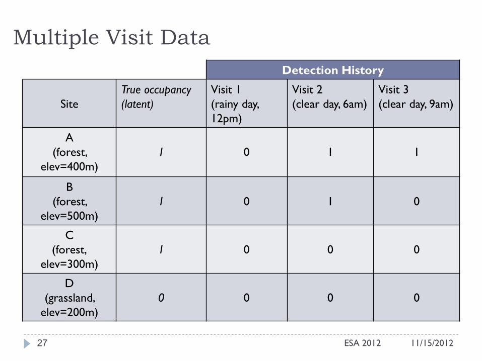
Multiple Visit Data
27
Detection History
Site
True occupancy
(latent)
Visit 1
(rainy day,
12pm)
Visit 2
(clear day, 6am)
Visit 3
(clear day, 9am)
A
(forest,
elev=400m)
1
0
1
1
B
(forest,
elev=500m)
1
0
1
0
C
(forest,
elev=300m)
1
0
0
0
D
(grassland,
elev=200m)
0
0
0
0
11/15/2012 ESA 2012
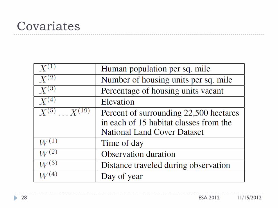
Covariates
11/15/2012 ESA 2012 28

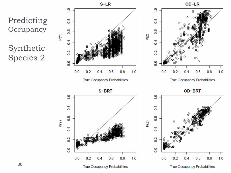
Synthetic Species 2
𝐹 and 𝐺 nonlinear
log𝑜𝑖
1 − 𝑜𝑖= −2 𝑥𝑖
12
+ 3 𝑥𝑖2
2− 2𝑥𝑖
3
log𝑑𝑖𝑡
1 − 𝑑𝑖𝑡= exp(−0.5𝑤𝑖𝑡
4) + sin(1.25𝑤𝑖𝑡
1+ 5)
11/15/2012 ESA 2012 29
11/15/2012 ESA 2012
Predicting Occupancy
Synthetic
Species 2
30
Open Problems
ESA 2012 31
Sometimes the OD model finds trivial solutions
Detection probability = 0 at many sites, which allows the Occupancy model complete freedom at those sites
Occupancy probability constant (0.2)
Log likelihood for latent variable models suffers from local minima
Proper initialization?
Proper regularization?
Posterior regularization?
How much data do we need to fit this model?
Can we detect when the model has failed?
11/15/2012