PHYSICAL REVIEW A 92, 013633 (2015)

Bright solitons in a two-dimensional spin-orbit-coupled dipolar Bose-Einstein condensate

Yong Xu,1 Yongping Zhang,2 and Chuanwei Zhang1,*

1Department of Physics, The University of Texas at Dallas, Richardson, Texas 75080, USA2Quantum Systems Unit, OIST Graduate University, Onna, Okinawa 904-0495, Japan

(Received 8 May 2015; published 27 July 2015)

We study a two-dimensional spin-orbit-coupled dipolar Bose-Einstein condensate with repulsive contactinteractions by both the variational method and the imaginary-time evolution of the Gross-Pitaevskii equation.The dipoles are completely polarized along one direction in the two-dimensional plane to provide an effectiveattractive dipole-dipole interaction. We find two types of solitons as the ground states arising from such attractivedipole-dipole interactions: a plane-wave soliton with a spatially varying phase and a stripe soliton with a spatiallyoscillating density for each component. Both types of solitons possess smaller size and higher anisotropy than thesoliton without spin-orbit coupling. Finally, we discuss the properties of moving solitons, which are nontrivialbecause of the violation of Galilean invariance.

DOI: 10.1103/PhysRevA.92.013633 PACS number(s): 03.75.Lm, 03.75.Mn, 71.70.Ej

I. INTRODUCTION

Ever since the first achievement of Bose-Einstein conden-sates (BECs) in ultracold atomic gases [1–3], matter wavesolitons in these systems have been the central focus ofmany experiments and theory [4]. Solitons that keep theirshape while traveling are the result of the interplay betweennonlinearity and dispersion. In BECs, nonlinearity usuallyoriginates from short-range collisional interactions betweenatoms, which can be readily tuned via Feshbach resonances [5].In general, there are two types of solitons: a bright solitonwith a density bump and a dark soliton with a density notchas well as a phase jump [4]. For pure contact interactions, abright and a dark soliton can emerge, respectively, when theinteractions are attractive or repulsive. Both these solitons havebeen experimentally observed in cold atoms [6–14]. However,for these contact attractive interactions, bright solitons canonly exist in one dimension, but not in two dimensions, wherethe states either collapse or expand [15].

Different from the local nonlinearity resulting from contactinteractions, the nonlocal nonlinearity, in particular, the nonlin-earity introduced by the dipole-dipole interaction, can stabilizea two-dimensional (2D) bright soliton [16,17]. The dipoleinteraction is long range and anisotropic with the strengthand sign (i.e., repulsive or attractive) depending on the dipoleorientation. When an external rotating magnetic field is appliedto reverse the sign of the interaction [18] or the dipoles arecompletely polarized in a 2D plane [19], the dipolar interactioncan become attractive and 2D bright solitons can therefore bestabilized under appropriate conditions (i.e., the ground state ofthe system is a bright soliton with a localized density profile).It is essential to note that although the relevant interaction inmost experiments with cold atomic gases is contact, increasinginterest has been focused on the atoms with large magneticmoments that possess dipole-dipole interactions [17,20,21]. Infact, the Bose-Einstein condensation of several dipolar atomssuch as chromium [22–24], dysprosium [25], and erbium [26]and the degeneracy of a dipolar Fermi gas [27,28] have beenobserved in experiments.

*chuanwei.zhang@utdallas.edu

Recently, the spin-orbit coupling between two hyperfinestates of cold atoms has been experimentally engineered[29–34]. This achievement has ignited tremendous interestin this field because of the dramatic change in the single-particle dispersion (induced by spin-orbit coupling), whichin conjunction with the interaction leads to many exoticsuperfluids [35–46] (also see [47–54] for reviews). Suchchange in dispersion also results in exotic solitons even whenthe interaction is contact (without dipole-dipole interactions),including 1D bright solitons [55–61] for a BEC with attractivecontact interactions, 1D dark [62,63] and gap solitons [64–66]for a BEC with repulsive contact interactions, and 1D darksolitons for Fermi superfluids [67,68]. These solitons exhibitunique features that are absent without spin-orbit coupling, forinstance, the plane-wave profile with a spatially varying phaseand the stripe profile with a spatially oscillating density forBECs, as well as the presence of Majorana fermions inside asoliton for Fermi superfluids. Also, the violation of Galileaninvariance [56,69,70] by spin-orbit coupling dictates that thestructure of solitons changes with their velocities.

On the other hand, spin-orbit-coupled BECs with dipole-dipole interactions [71–74] have also been explored andintriguing quasicrystals [75] as well as meron states [76]have been found (these ground states are extended and notlocalized bright solitons). However, whether a soliton canexist in such BECs in two dimensions with both long-rangedipole-dipole interactions and spin-orbit dispersion has not yetbeen investigated.

In this paper we examine the existence and properties of abright soliton in a two-species spin-orbit-coupled dipolar BECin two dimensions with repulsive contact interactions via boththe variational method and the imaginary-time evolution of theGross-Pitaevskii equation (GPE). The dipoles are completelyoriented along the y direction in the 2D plane [i.e., the (x,y)plane] in order to provide an effective attractive dipole-dipoleinteraction. Due to such attractive interactions, we find twotypes of solitons: a plane-wave soliton (when the repulsiveintraspecies contact interaction is larger than the repulsiveinterspecies one) and a stripe soliton (when the interspeciesone is larger). These 2D solitons are the ground states ofthe system and they cannot exist as the ground states of asystem with purely attractive contact interactions (no dipole)

1050-2947/2015/92(1)/013633(9) 013633-1 ©2015 American Physical Society

YONG XU, YONGPING ZHANG, AND CHUANWEI ZHANG PHYSICAL REVIEW A 92, 013633 (2015)

and spin-orbit coupling. Such solitons are highly anisotropicand their size is also reduced by spin-orbit coupling. Finally,we study the moving solitons, which are nontrivial becauseof the lack of Galilean invariance. The size of a soliton firstincreases and then decreases with the rise of the velocity andthis change is anisotropic. The moving soliton also tends to beplane wave even when its stationary counterpart has the stripestructure.

The paper is organized as follows. In Sec. II we introducethe energy functional and the time-dependent GPE, which areused to describe a spin-orbit-coupled dipolar BEC. In Sec. IIIwe calculate the ground states that are bright solitons byperforming the minimization of the energy of the variationalansatz wave functions and an imaginary-time evolution of theGPE. The properties of such soliton are also explored by theformer method. Then we study the nontrivial moving solitonsin Sec. IV. Finally, we summarize in Sec. V.

II. MODEL

We consider a Rashba-type spin-orbit-coupled BEC [47,51]and write its single-particle Hamiltonian as

Hs = p2

2m+ 1

2mω2

⊥ρ2 + 1

2mω2

zz2 + λ(p × σ ) · ez, (1)

where ρ =√

x2 + y2, p = −i�∇ is the momentum operator,m is the atom mass, λ is the spin-orbit coupling strength, σ

are Pauli matrices, ez is a unit vector along the z direction, andω⊥ (ωz) is the trap frequency in the (x,y) plane (along the z

direction). Here we assume that �ωz is much larger than �ω⊥and the mean-field interaction so that the atoms are frozento the ground state in the z direction. Given that a soliton isstudied, we thus set ω⊥ = 0.

When the s-wave contact and dipole-dipole interactionsare involved, the energy functional of a 2D condensate can bewritten as

E =∫

dr[�(r)†Hs�(r) + 1

2g(|�↑|4 + |�↓|4)

+ g12|�↑|2|�↓|2]

+ Edd, (2)

where the condensate wave function �(r) = [�↑(r),�↓(r)]T

with two pseudospin components �↑ (↓)(r) and g =4π�

2a/√

2πlzm and g12 = 4π�2a12/

√2πlzm are the in-

traspecies and interspecies contact interaction strengths, re-spectively, with the intraspecies and interspecies s-wavescattering length being a and a12 and the characteristic lengthalong z being lz = √

�/mωz. Here Hs = −�2(∂2

x + ∂2y )/2m −

i�λ(∂xσy − ∂yσx) is the 2D single-particle Hamiltonian andthe third dimension has been integrated out. For dipole-dipoleinteractions, we only consider the density-density interaction,which is dominant when a two-subspace (i.e., two pseudospinstates) of a large spin atom (e.g., dysprosium) is considered.We also assume that the dipoles are all oriented along the y

direction, thus

Edd = gd

2

1

(2π )2

∫dkρkρ−kUd (klz), (3)

where the Fourier transform of the total density is ρk =∫dre−ik·r(|�↑|2 + |�↓|2) and U (k) is given by [18]

Ud (klz) = −√

2π + 3πlzk2ye

k2l2z /2 erfc(klz/

√2)

k, (4)

with erfc being the complementary error function. Here gd =μ0μ

2/6πlz characterizes the strength of the dipole-dipoleinteraction where μ is the magnetic dipolar moment and μ0 isthe permeability of the free space. We note that this head-to-taildipole configuration that can be attractive is different from thehead-to-head configuration in Ref. [75] that is repulsive.

The dynamical behavior of a BEC can be described by thetime-dependent GPE

i�∂�(r)

∂t= Hs�(r) + gG�(r) + gdUd (r)�(r), (5)

where the contact interaction matrix is

G =(

|�↑|2 + g12

g|�↓|2 0

0 |�↓|2 + g12

g|�↑|2

)(6)

and the dipolar interaction potential is

Ud (r) = 1

(2π )2

∫dkeik·rρ(k)Ud (klz). (7)

For numerical simulation, we choose �ωz, lz, and 1/ωz asthe units of energy, length, and time, respectively, and thedimensionless energy per atom hence reads

E =∫

dr[(r)†Hs(r) + 1

2γ (|↑|4 + |↓|4)

+ γ12|↑|2|�↓|2]

+ γd

2(2π )2

∫dknkn−kUd (k), (8)

where Hs = −(∂2x + ∂2

y )/2 − iα(∂xσy − ∂yσx), α = λ/ωxlz,

γ = 2√

2πN0a/lz, γ12 = 2√

2πN0a12/lz with the total parti-cle number N0, γd = 2N0ad/ lz with ad = mμ0μ

2/12π�2, and

nk = ∫dre−ik·r(|↑|2 + |↓|2). The wave function is normal-

ized to 1 [i.e.,∫

dr(|↑|2 + |↓|2) = 1]. The dimensionlesstime-dependent GPE reads

i∂(r)

∂t= Hs(r) + γG(r)

+ γd

(2π )2

∫dkeik·rn(k)Ud (k)(r), (9)

where

G =(

|↑|2 + γ12

γ|↓|2 0

0 |↓|2 + γ12

γ|↑|2

). (10)

III. STATIONARY BRIGHT SOLITONS

To shed light on the structure of a soliton, we start froma Rashba spin-orbit-coupled single-particle system in theabsence of interactions in a free space and write its momentumspace dispersion as

E(k) = k2

2± αk, (11)

013633-2

BRIGHT SOLITONS IN A TWO-DIMENSIONAL SPIN- . . . PHYSICAL REVIEW A 92, 013633 (2015)

with two branches labeled by the helicity ±, which is the

eigenvalue of (kxσy − kyσx)/k, where k =√

k2x + k2

y . Clearly,

the ground state is degenerate with the energy being −α2/2when the momenta lie in the k = |α| ring. This is differentfrom the case without spin-orbit coupling where the groundstate only occurs at k = 0. In this single-particle case, anysuperposition of the states in the ring is also its ground state.Yet this is not the case when the repulsive contact interaction isinvolved. The ground state possesses either a single momentum(i.e., plane-wave phase) when γ12/γ < 1 or two oppositemomenta (i.e., stripe phase) when γ12/γ > 1 [36]. When thedipolar interaction is turned on, one may expect two typesof ground states—plane-wave and stripe solitons—due to thiseffective long-range attractive interaction along with contactrepulsive interaction.

To examine whether the ground state can indeed be abright soliton in the spin-orbit-coupled dipolar BECs, we firstconsider a plane-wave soliton variational ansatz

P =(

0(x0/2)

−0(−x0/2)

)exp(−iJp · r), (12)

where

0(x0) = (axay)1/4

√2π

e−[ax (x−x0)2+ayy2]/2. (13)

Here r = xex + yey with unit vectors ex and ey along the x

and y directions, respectively, Jp = Jpey is the wave vectorof the plane-wave soliton, lν = 1/

√aν with ν = x,y is the

size of the soliton, and x0 is the separation distance betweentwo components. When x0 = 0, this state is an eigenstateof pyσx multiplied by a Gaussian profile 0(0) and Jp = α

yields the minimum energy. In fact, x0 is usually nonzerobecause of a force acting on the BEC by spin-orbit couplingF = α2(p × ez)σz [40,77], which is opposite along the x

direction when p (here Jp) is along the y direction.In writing down the ansatz (12), we have assumed that the

wave vector of the plane-wave soliton is in the y direction.The prerequisite of this assumption is that the rotationsymmetry [40,41] about the z axis has been broken by thedipole-dipole interaction. Indeed, without the dipole-dipoleinteraction, this state with Jp along y is not special and otherstates with Jp along other directions are degenerate with it.For example, the state with Jp along y has the same energyas a state with Jp along x. Yet, with the specific dipole-dipoleinteraction arising from the dipoles entirely oriented alongy, the symmetry is broken and the ground state should beelongated along y (ax > ay) so as to provide an effectiveattractive interaction because of the head-to-tail configurationof polarized dipoles. This elongated configuration allows theexistence of a 2D soliton [19] and also requires the wave vectorto be along y [78].

Although the wave vector Jp of the ground state is along y,there are still two options: negative and positive directions interms of the time-reversal symmetry T (i.e., −iσyK with thecomplex conjugate operator K). Specifically, the state P 2 =T P is degenerate with P . In the absence of interactions,all superposition states of P and P 2,

PS = |cos θ |P + |sin θ |eiϕP 2, (14)

are degenerate. This degeneracy may be broken by theinteraction so that the ground state is either P or P 2 or acertain superposition state of them; however, this degeneracybreaking should not happen at γ12/γ = 1 since the interactionenergy only depends on the total density, which is independentof θ and ϕ. This gives us an intuitive understanding thatγ12/γ = 1 may separate the plane-wave state (|cos θ | = 0or 1) and the stripe one (|cos θ | = |sin θ |), similar to thehomogenous spin-orbit-coupled BEC [36] without dipole-dipole interactions. For the stripe state, we note that ϕ = 0,π

corresponds to the ground state as the energy contributed by ϕ

is −γ12√

axaye−(axx

20 /2+2J 2

p/ay ) cos(2ϕ)/16π [79].To evaluate the variational parameters ax , ay , x0, Jp, and θ ,

we minimize the energy E after substituting PS from Eq. (14)in Eq. (8). Indeed, the calculated variational solutions revealthat there are two types of ground states: plane-wave stateswhen γ12/γ < 1 and stripe states when γ12/γ > 1. Theseground states are bright solitons with localized density profilesas shown in Fig. 1; we therefore call these ground statesplane-wave solitons and stripe solitons. In Figs. 1(a1)–1(el),the density and phase profiles of a typical plane-wave soliton(we choose θ = ϕ = 0) are presented and the stripe structureof the phase of both two components reveals the plane-wavefeature. The soliton is highly elongated along the y directionand the centers of two components are spatially separatedalong the x direction because of nonzero x0. To confirmthat this variational solution can qualitatively characterize theground state of the system, we numerically compute the groundstate by an imaginary-time evolution of the GPE (9). Thisexact numerical solution also concludes that γ12/γ < 1 yieldsthe plane-wave soliton, while γ12/γ > 1 the stripe one. InFigs. 1(a2)–1(e2), we also plot the corresponding density andphase profiles of the Gross-Pitaevskii-obtained plane-wavesoliton. The variational ansatz is in qualitative agreement withit given the separated centers and the plane-wave varying phasethat both states possess. Yet the shape of the soliton obtainedby the imaginary-time evolution deviates slightly from theGaussian and the size is also slightly smaller.

When θ = π/4 and ϕ = 0, PS is a stripe soliton state witha density oscillation along the y direction for each component.In addition, there is no stripe for the total density. Along the x

direction, two components are not spatially separated and thephase for the spin ↑ reverses suddenly across x = 0. Followingthese properties by replacing [0(x0/2) + 0(−x0/2)]/

√2

with cos(Jxx)0(0) and [0(x0/2) − 0(−x0/2)]/√

2 withsin(Jxx)0(0) in Eq. (14), we obtain another better variationalansatz for the stripe soliton

S = �0(0), (15)

where

� =(

cos(Jyy) cos(Jxx) − i sin(Jyy) sin(Jxx)

cos(Jyy) sin(Jxx) + i sin(Jyy) cos(Jxx)

), (16)

with the variational parameters Jx and Jy . The period of thestripe along the y direction is π/Jy . Interestingly, this stripesoliton corresponds to four points (±Jx,±Jy) in momentumspace instead of traditional two points [56] when Jx = 0, if wedo not consider the Gaussian profile 0.

013633-3

YONG XU, YONGPING ZHANG, AND CHUANWEI ZHANG PHYSICAL REVIEW A 92, 013633 (2015)

2

4

1

2

3

y

−10

−5

0

5

10

1

2

3

0

×10−2 ×10−2 ×10−2 π(b1) n↓ (d1) arg(Φ↑) (e1) arg(Φ↓)(a1) n↑

−π

(c1) n↑+n↓

y

−1.1 0 1.5

−10

−5

0

5

10

−1.5 0 1.1x

−1.3 0 1.3 −1.1 0 0 1.3

1

2

3

4

1

2

3

4

2

4

6

8

0

×10−2 ×10−2 ×10−2 π(a2) n↑ (d2) arg(Φ↑) (e2) arg(Φ↓)(b2) n↓

−π−1.51.5

(c2) n↑+n↓

y

−10

−5

0

5

10

1

2

3

1

2

3

1

1

2

3

0

×10−2 ×10−2 ×10−2 π(a3) n↑ (b3) n↓ (d3) arg(Φ↑) (e3) arg(Φ↓)

−π

(c3) n↑+n↓

y

−1.5 0 1.5

−10

−5

0

5

10

−1.5 0 1.5x

−1.5 0 1.5 −1.5 0 1.5 −1.5 0 1.5

2

4

2

4

2

2

4

0

(a4) n↑ (b4) n↓ (d4) arg(Φ↑) (e4) arg(Φ↓)×10−2 ×10−2 ×10−2 π

(c4) n↑+n↓

−π

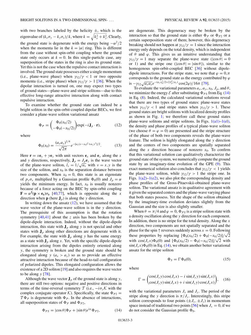
FIG. 1. (Color online) Profiles of the density n↑,↓ = |↑,↓|2 of (a) spin ↑ and (b) spin ↓, (c) the total density n↑ + n↓, the phase of (d) spin ↑and (e) spin ↓ for (a1)–(e1) and (a2)–(e2) a plane-wave soliton with γ12 = 6 and (a3)–(e3) and (a4)–(e4) a stripe soliton with γ12 = 10. (a1)–(el)and (a3)–(e3) The solitons are obtained by the variational method. (a2)–(e2) and (a4)–(e4) The solitons are calculated by the imaginary-timeevolution of the GPE (9). The dashed white line labels the x = 0 line. Here γ = 8, γd/γ = 0.67, and α = 2.

We calculate the variational parameters of stripe solitonsby performing the minimization of the energy E in Eq. (8)where is replaced with S . The density and phase profilesof a typical stripe soliton calculated by this method aredisplayed in Figs. 1(a3)–1(e3). Evidently, the density of eachcomponent exhibits the stripe structure, while the total densitydoes not. The phase of spin ↑ along the y direction varieslike a plane wave, but reverses across x = 0 due to thepresence of sin(Jxx) in the imaginary part. The phase of spin↓ exhibits the phase rotationlike vortices around x = 0 andy = nπ/Jy with an integer n; around these points, the wavefunction S↓ is proportional to (−1)n[Jxx + i(Jyy − nπ )]and the corresponding density of spin ↓ is extremely low.Moreover, in Figs. 1(a4)–1(e4), we plot the density and phase

profiles of the corresponding stripe soliton obtained by theimaginary-time evolution of the GPE; comparing these figureswith Figs. 1(a3)–1(e3) shows that the stripe variational ansatzis qualitatively consistent with the Gross-Pitaevskii results.

To study the properties of a soliton with respect to dipole-dipole interactions γd , we evaluate the variational parametersof both the plane-wave and stripe solitons by the variationalmethod and plot them in Fig. 2 as γd/γ varies. Clearly, withincreasing γd/γ , ax and ay increase monotonically becauseof the enhanced effective attractive interaction, indicating thatthe size lx and ly of the soliton decrease monotonically. Wenote that as γd/γ increases further, the soliton can collapseso that both ax and ay diverge. For the plane-wave soliton,ax and ay are slightly larger than the stripe soliton because

013633-4

BRIGHT SOLITONS IN A TWO-DIMENSIONAL SPIN- . . . PHYSICAL REVIEW A 92, 013633 (2015)

0

2

4

6

8

a x

0

0.1

0.2

0.3

0.4

a y 0.3 0.4 0.50

0.5

1

γd/γ

(ay/a

x)1/2

(b)(a)

0.3 0.4 0.5 0.60

0.5

1

1.5

2

γd/γ

0.3 0.4 0.5 0.6

−3

−2.5

−2

γd/γ

ener

gy

(d)

x0

Jx

Jy

Jp

(c)

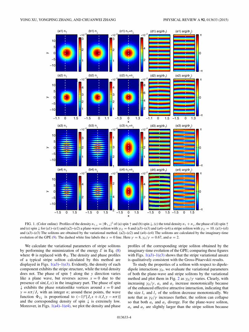
FIG. 2. (Color online) Plot of (a) ax and (b) ay as a function ofγd/γ for the plane-wave solitons (dotted blue line), stripe solitons(dashed green line), and traditional solitons (solid red line) withoutspin-orbit coupling. The aspect ratio

√ay/ax of a soliton is displayed

in the inset of (b). (c) Variational parameters with respect γd/γ ,associated with x0 (dash-dotted blue line) and Jp (dashed blue line)for the plane-wave soliton and Jx (solid green line) and Jy (dottedgreen line) for the stripe soliton. (d) Total energy of the variationalansatz wave function and the wave function numerically obtained bythe imaginary-time evolution of the GPE for both plane-wave andstripe solitons. The solid green line (stripe soliton) and dashed blueline (plane-wave soliton) correspond to the variational results, whilethe green circles and blue squares correspond to the Gross-Pitaevskiiresults. Here α = 2, γ = 8, and γ12 = 6 (γ12 = 10) for the plane-wave(stripe) soliton.

of the smaller contact interaction of the former. Moreover,compared with the soliton without spin-orbit coupling [redline in Figs. 2(a) and 2(b)], ax and ay for both the plane-waveand stripe solitons are much larger, implying that the size ofsolitons can be reduced by spin-orbit coupling. Also, thesesolitons are highly anisotropic with the much smaller aspectratio

√ay/ax as shown in the inset of Fig. 2(b). To elucidate

the reason, we explicitly write that single-particle energy ofthe plane-wave variational ansatz in Eq. (12), which resultsfrom the presence of x0 and Jp,

EPWs = 1

2J 2p − αe−x2

0 ax/4(Jp + 1

2axx0). (17)

The minimization of EPWs with respect to x0 and Jp for fixed

ax yields

x0 =−Jp +

√J 2

p + 2ax

ax

, (18)

Jp = αe−x20 ax/4. (19)

For ax = 0, the energy is independent of x0 and Jp = α, whilefor ax �= 0, both x0 and Jp decrease slightly with increasing ax

0 1 2 30

0.5

1

1.5

2

ax

0 1 2 3

−2.6

−2.4

−2.2

−2

ax

E Stripes

Es PW

(a) (b)

x0

Jp

Jy

Jx

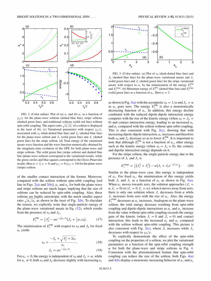
FIG. 3. (Color online) (a) Plot of x0 (dash-dotted blue line) andJp (dashed blue line) for the plane-wave variational ansatz and Jx

(solid green line) and Jy (dotted green line) for the stripe variationalansatz with respect to ax by the minimization of the energy EPW

s

and Estripes . (b) Minimum energy of EPW

s (dotted blue line) and Estripes

(solid green line) as a function of ax . Here α = 2.

as shown in Fig. 3(a) with the asymptotic x0 = 1/α and Jp = α

as ax goes zero. The energy EPWs is also a monotonically

decreasing function of ax . In addition, this energy declinecombined with the reduced dipole-dipole interaction energycompetes with the rise of the kinetic energy (when x0 = Jp =0) and contact interaction energy, leading to an increased ax

and ay compared with the soliton without spin-orbit coupling.This is also consistent with Fig. 2(c), showing that withincreasing dipole-dipole interaction, ax increases and thereforeboth x0 and Jp decrease so as to lower EPW

s . It is important tonote that although EPW

s is not a function of ay , other energysuch as the kinetic energy (when x0 = Jp = 0), the contact,and dipolar interaction energy depends on it.

For the stripe soliton, the single-particle energy due to thepresence of Jx and Jy is

Estripes = 1

2

(J 2

x + J 2y

) − α(Jx + Jye

−J 2x /ax

). (20)

Similar to the plane-wave case, this energy is independentof ay . For fixed ax , the minimization of this energy yieldsboth Jx and Jy as a function of ax as shown in Fig. 3(a).When ax moves towards zero, the solution approaches (Jx =α,Jy = 0) or (Jx = 0,Jy = α); when it moves away from zero,there is only one solution where Jy decreases from α whileJx increases from zero with the rise of ax . Also, the energyE

stripes decreases as ax increases. Analogous to the plane-wave

soliton, the total energy decrease resulting from spin-orbitcoupling and dipole-dipole interactions as ax and ay increasefrom the value without spin-orbit coupling exceeds the energygain of the kinetic (when Jx = 0 and Jy = 0) and contactinteraction; this leads to the increased ax and ay comparedwith the soliton without spin-orbit coupling. This picture isalso consistent with Fig. 2(c), where Jx increases while Jy

decreases with respect to γd/γ .To explicitly demonstrate the effect of the spin-orbit

coupling on the properties of a soliton, we plot the variationalparameters as a function of the spin-orbit coupling strengthα for both the plane-wave and stripe solitons in Fig. 4.Consistent with the aforementioned feature that spin-orbitcoupling can reduce the size of the soliton, both Figs. 4(a)and 4(b) display a monotonic increasing behavior of ax and ay

013633-5

YONG XU, YONGPING ZHANG, AND CHUANWEI ZHANG PHYSICAL REVIEW A 92, 013633 (2015)

0

2

4

6

a x

0

0.02

0.04

0.06

0.08

0.1

a y2 40

0.1

0.2

(ay/a

x)1/2

(a) (b)

1 2 3 4 50

1

2

3

4

5

α1 2 3 4 5

−0.15

−0.1

−0.05

0

α

ener

gy+

α2 /2

Jx

Jy

x0

Jp

(c) (d)

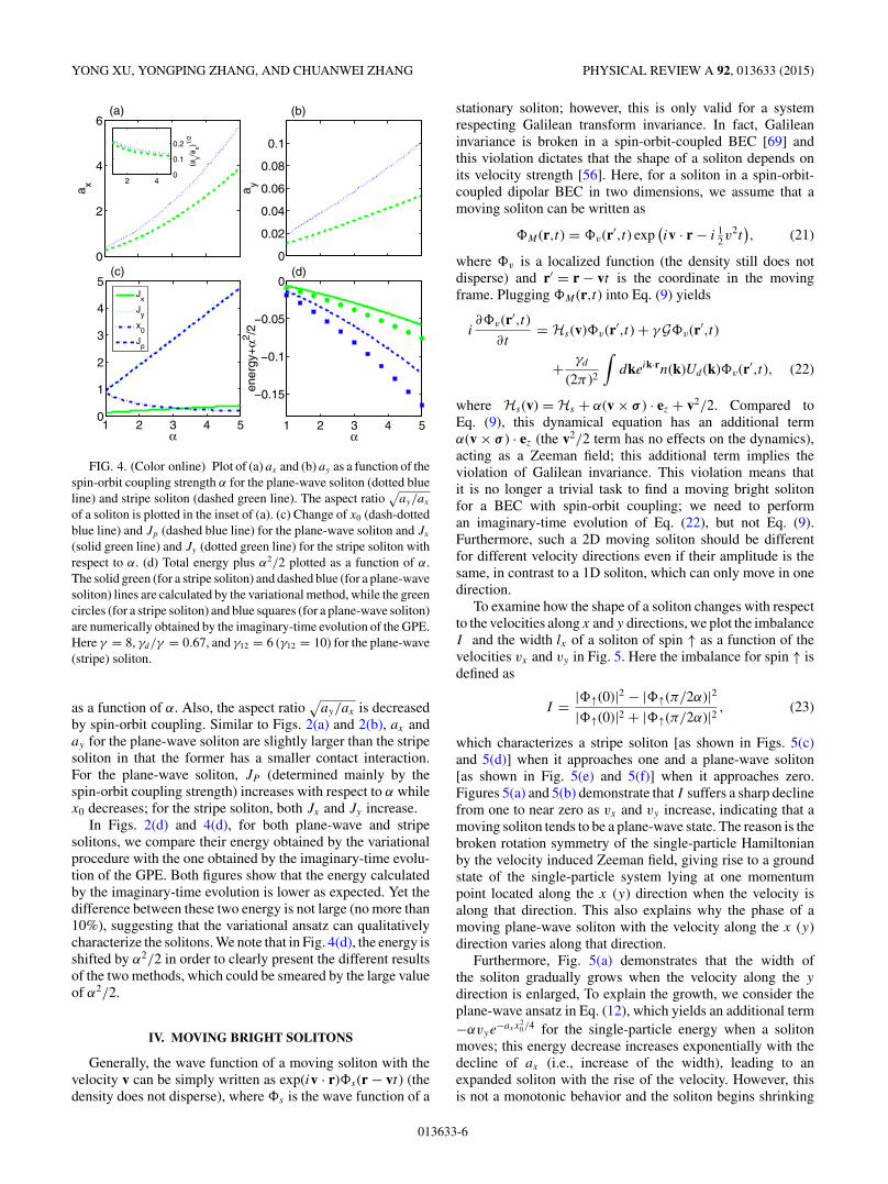
FIG. 4. (Color online) Plot of (a) ax and (b) ay as a function of thespin-orbit coupling strength α for the plane-wave soliton (dotted blueline) and stripe soliton (dashed green line). The aspect ratio

√ay/ax

of a soliton is plotted in the inset of (a). (c) Change of x0 (dash-dottedblue line) and Jp (dashed blue line) for the plane-wave soliton and Jx

(solid green line) and Jy (dotted green line) for the stripe soliton withrespect to α. (d) Total energy plus α2/2 plotted as a function of α.The solid green (for a stripe soliton) and dashed blue (for a plane-wavesoliton) lines are calculated by the variational method, while the greencircles (for a stripe soliton) and blue squares (for a plane-wave soliton)are numerically obtained by the imaginary-time evolution of the GPE.Here γ = 8, γd/γ = 0.67, and γ12 = 6 (γ12 = 10) for the plane-wave(stripe) soliton.

as a function of α. Also, the aspect ratio√

ay/ax is decreasedby spin-orbit coupling. Similar to Figs. 2(a) and 2(b), ax anday for the plane-wave soliton are slightly larger than the stripesoliton in that the former has a smaller contact interaction.For the plane-wave soliton, JP (determined mainly by thespin-orbit coupling strength) increases with respect to α whilex0 decreases; for the stripe soliton, both Jx and Jy increase.

In Figs. 2(d) and 4(d), for both plane-wave and stripesolitons, we compare their energy obtained by the variationalprocedure with the one obtained by the imaginary-time evolu-tion of the GPE. Both figures show that the energy calculatedby the imaginary-time evolution is lower as expected. Yet thedifference between these two energy is not large (no more than10%), suggesting that the variational ansatz can qualitativelycharacterize the solitons. We note that in Fig. 4(d), the energy isshifted by α2/2 in order to clearly present the different resultsof the two methods, which could be smeared by the large valueof α2/2.

IV. MOVING BRIGHT SOLITONS

Generally, the wave function of a moving soliton with thevelocity v can be simply written as exp(iv · r)s(r − vt) (thedensity does not disperse), where s is the wave function of a

stationary soliton; however, this is only valid for a systemrespecting Galilean transform invariance. In fact, Galileaninvariance is broken in a spin-orbit-coupled BEC [69] andthis violation dictates that the shape of a soliton depends onits velocity strength [56]. Here, for a soliton in a spin-orbit-coupled dipolar BEC in two dimensions, we assume that amoving soliton can be written as

M (r,t) = v(r′,t) exp(iv · r − i 1

2v2t), (21)

where v is a localized function (the density still does notdisperse) and r′ = r − vt is the coordinate in the movingframe. Plugging M (r,t) into Eq. (9) yields

i∂v(r′,t)

∂t= Hs(v)v(r′,t) + γGv(r′,t)

+ γd

(2π )2

∫dkeik·rn(k)Ud (k)v(r′,t), (22)

where Hs(v) = Hs + α(v × σ ) · ez + v2/2. Compared toEq. (9), this dynamical equation has an additional termα(v × σ ) · ez (the v2/2 term has no effects on the dynamics),acting as a Zeeman field; this additional term implies theviolation of Galilean invariance. This violation means thatit is no longer a trivial task to find a moving bright solitonfor a BEC with spin-orbit coupling; we need to performan imaginary-time evolution of Eq. (22), but not Eq. (9).Furthermore, such a 2D moving soliton should be differentfor different velocity directions even if their amplitude is thesame, in contrast to a 1D soliton, which can only move in onedirection.

To examine how the shape of a soliton changes with respectto the velocities along x and y directions, we plot the imbalanceI and the width lx of a soliton of spin ↑ as a function of thevelocities vx and vy in Fig. 5. Here the imbalance for spin ↑ isdefined as

I = |↑(0)|2 − |↑(π/2α)|2|↑(0)|2 + |↑(π/2α)|2 , (23)

which characterizes a stripe soliton [as shown in Figs. 5(c)and 5(d)] when it approaches one and a plane-wave soliton[as shown in Fig. 5(e) and 5(f)] when it approaches zero.Figures 5(a) and 5(b) demonstrate that I suffers a sharp declinefrom one to near zero as vx and vy increase, indicating that amoving soliton tends to be a plane-wave state. The reason is thebroken rotation symmetry of the single-particle Hamiltonianby the velocity induced Zeeman field, giving rise to a groundstate of the single-particle system lying at one momentumpoint located along the x (y) direction when the velocity isalong that direction. This also explains why the phase of amoving plane-wave soliton with the velocity along the x (y)direction varies along that direction.

Furthermore, Fig. 5(a) demonstrates that the width ofthe soliton gradually grows when the velocity along the y

direction is enlarged, To explain the growth, we consider theplane-wave ansatz in Eq. (12), which yields an additional term−αvye

−axx20 /4 for the single-particle energy when a soliton

moves; this energy decrease increases exponentially with thedecline of ax (i.e., increase of the width), leading to anexpanded soliton with the rise of the velocity. However, thisis not a monotonic behavior and the soliton begins shrinking

013633-6

BRIGHT SOLITONS IN A TWO-DIMENSIONAL SPIN- . . . PHYSICAL REVIEW A 92, 013633 (2015)

0 5 100

1

2

3

4

vx

0 5 100

0.5

1

1.5

vy

0 0.1 0.20

0.5

1

0 0.50

2

4

(a) (b)lx

I

−0.6 0 0.6

−5

0

5

−0.600.6 −5 0 5

−5

0

5

−5 0 5−0.6 0 0.6

−5

0

5

−

−0.6 0 0.6−0.6 0 0.6

−5

0

5

−

−0.6 0 0.6

(c) vx=0,v

y=0 (d) v

x=0,v

y=0.015 (e) v

x=0,v

y=0.2 (f) v

x=0.2,v

y=0

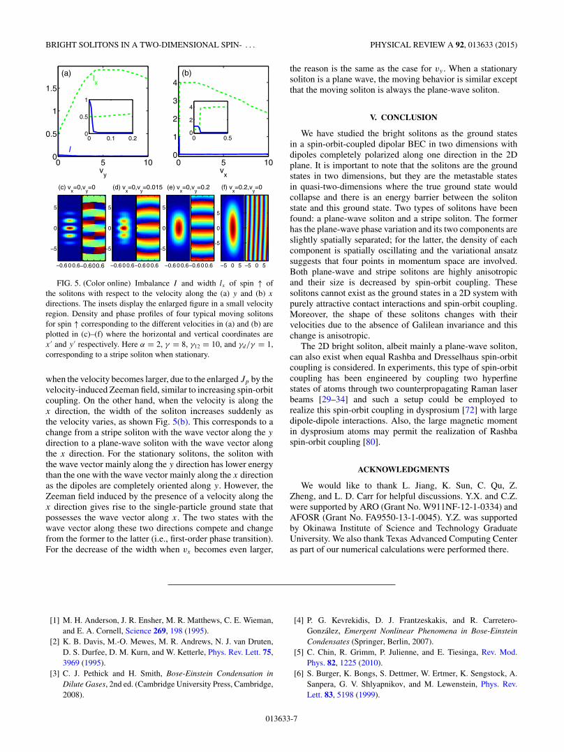
FIG. 5. (Color online) Imbalance I and width lx of spin ↑ ofthe solitons with respect to the velocity along the (a) y and (b) x

directions. The insets display the enlarged figure in a small velocityregion. Density and phase profiles of four typical moving solitonsfor spin ↑ corresponding to the different velocities in (a) and (b) areplotted in (c)–(f) where the horizontal and vertical coordinates arex ′ and y ′ respectively. Here α = 2, γ = 8, γ12 = 10, and γd/γ = 1,corresponding to a stripe soliton when stationary.

when the velocity becomes larger, due to the enlarged Jp by thevelocity-induced Zeeman field, similar to increasing spin-orbitcoupling. On the other hand, when the velocity is along thex direction, the width of the soliton increases suddenly asthe velocity varies, as shown Fig. 5(b). This corresponds to achange from a stripe soliton with the wave vector along the y

direction to a plane-wave soliton with the wave vector alongthe x direction. For the stationary solitons, the soliton withthe wave vector mainly along the y direction has lower energythan the one with the wave vector mainly along the x directionas the dipoles are completely oriented along y. However, theZeeman field induced by the presence of a velocity along thex direction gives rise to the single-particle ground state thatpossesses the wave vector along x. The two states with thewave vector along these two directions compete and changefrom the former to the latter (i.e., first-order phase transition).For the decrease of the width when vx becomes even larger,

the reason is the same as the case for vy . When a stationarysoliton is a plane wave, the moving behavior is similar exceptthat the moving soliton is always the plane-wave soliton.

V. CONCLUSION

We have studied the bright solitons as the ground statesin a spin-orbit-coupled dipolar BEC in two dimensions withdipoles completely polarized along one direction in the 2Dplane. It is important to note that the solitons are the groundstates in two dimensions, but they are the metastable statesin quasi-two-dimensions where the true ground state wouldcollapse and there is an energy barrier between the solitonstate and this ground state. Two types of solitons have beenfound: a plane-wave soliton and a stripe soliton. The formerhas the plane-wave phase variation and its two components areslightly spatially separated; for the latter, the density of eachcomponent is spatially oscillating and the variational ansatzsuggests that four points in momentum space are involved.Both plane-wave and stripe solitons are highly anisotropicand their size is decreased by spin-orbit coupling. Thesesolitons cannot exist as the ground states in a 2D system withpurely attractive contact interactions and spin-orbit coupling.Moreover, the shape of these solitons changes with theirvelocities due to the absence of Galilean invariance and thischange is anisotropic.

The 2D bright soliton, albeit mainly a plane-wave soliton,can also exist when equal Rashba and Dresselhaus spin-orbitcoupling is considered. In experiments, this type of spin-orbitcoupling has been engineered by coupling two hyperfinestates of atoms through two counterpropagating Raman laserbeams [29–34] and such a setup could be employed torealize this spin-orbit coupling in dysprosium [72] with largedipole-dipole interactions. Also, the large magnetic momentin dysprosium atoms may permit the realization of Rashbaspin-orbit coupling [80].

ACKNOWLEDGMENTS

We would like to thank L. Jiang, K. Sun, C. Qu, Z.Zheng, and L. D. Carr for helpful discussions. Y.X. and C.Z.were supported by ARO (Grant No. W911NF-12-1-0334) andAFOSR (Grant No. FA9550-13-1-0045). Y.Z. was supportedby Okinawa Institute of Science and Technology GraduateUniversity. We also thank Texas Advanced Computing Centeras part of our numerical calculations were performed there.

[1] M. H. Anderson, J. R. Ensher, M. R. Matthews, C. E. Wieman,and E. A. Cornell, Science 269, 198 (1995).

[2] K. B. Davis, M.-O. Mewes, M. R. Andrews, N. J. van Druten,D. S. Durfee, D. M. Kurn, and W. Ketterle, Phys. Rev. Lett. 75,3969 (1995).

[3] C. J. Pethick and H. Smith, Bose-Einstein Condensation inDilute Gases, 2nd ed. (Cambridge University Press, Cambridge,2008).

[4] P. G. Kevrekidis, D. J. Frantzeskakis, and R. Carretero-Gonzalez, Emergent Nonlinear Phenomena in Bose-EinsteinCondensates (Springer, Berlin, 2007).

[5] C. Chin, R. Grimm, P. Julienne, and E. Tiesinga, Rev. Mod.Phys. 82, 1225 (2010).

[6] S. Burger, K. Bongs, S. Dettmer, W. Ertmer, K. Sengstock, A.Sanpera, G. V. Shlyapnikov, and M. Lewenstein, Phys. Rev.Lett. 83, 5198 (1999).

013633-7

YONG XU, YONGPING ZHANG, AND CHUANWEI ZHANG PHYSICAL REVIEW A 92, 013633 (2015)

[7] J. Denschlag, J. E. Simsarian, D. L. Feder, C. W. Clark, L. A.Collins, J. Cubizolles, L. Deng, E. W. Hagley, K. Helmerson, W.P. Reinhardt, S. L. Rolston, B. I. Schneider, and W. D. Phillips,Science 287, 97 (2000).

[8] B. P. Anderson, P. C. Haljan, C. A. Regal, D. L. Feder, L. A.Collins, C. W. Clark, and E. A. Cornell, Phys. Rev. Lett. 86,2926 (2001).

[9] K. E. Strecker, G. B. Partridge, A. G. Truscott, and R. G. Hulet,Nature (London) 417, 150 (2002).

[10] L. Khaykovich, F. Schreck, G. Ferrari, T. Bourdel, J. Cubizolles,L. D. Carr, Y. Castin, and C. Salomon, Science 296, 1290 (2002).

[11] S. L. Cornish, S. T. Thompson, and C. E. Wieman, Phys. Rev.Lett. 96, 170401 (2006).

[12] B. Eiermann, T. Anker, M. Albiez, M. Taglieber, P. Treutlein,K.-P. Marzlin, and M. K. Oberthaler, Phys. Rev. Lett. 92, 230401(2004).

[13] C. Hamner, Y. Zhang, J. J. Chang, C. Zhang, and P. Engels,Phys. Rev. Lett. 111, 264101 (2013).

[14] J. H. V. Nguyen, P. Dyke, D. Luo, B. A. Malomed, and R. G.Hulet, Nat. Phys. 10, 918 (2014).

[15] The energy of a 2D system with contact interactions is ( �2

4m−

g

2π)/L2, where the first and second terms are, respectively, the

kinetic energy and contact attractive interaction (i.e., g > 0)energy, if the ground state is assumed to be e−(x2+y2)/2L2

/√

πL

with the size L of the state. When g < �2π/2m, the ground

state corresponds to L → ∞ (expansion instability); when g >

�2π/2m, L → 0 (collapse instability). See also Ref. [4].

[16] W. Krolikowski, O. Bang, J. J. Rasmussen, and J. Wyller,Phys. Rev. E 64, 016612 (2001).

[17] T. Lahaye, C. Menotti, L. Santos, M. Lewenstein, and T. Pfau,Rep. Prog. Phys. 72, 126401 (2009).

[18] P. Pedri and L. Santos, Phys. Rev. Lett. 95, 200404 (2005).[19] I. Tikhonenkov, B. A. Malomed, and A. Vardi, Phys. Rev. Lett.

100, 090406 (2008).[20] C. Ticknor, R. M. Wilson, and J. L. Bohn, Phys. Rev. Lett. 106,

065301 (2011).[21] M. A. Baranov, M. Dalmonte, G. Pupillo, and P. Zoller,

Chem. Rev. 112, 5012 (2012).[22] A. Griesmaier, J. Werner, S. Hensler, J. Stuhler, and T. Pfau,

Phys. Rev. Lett. 94, 160401 (2005).[23] T. Koch, T. Lahaye, J. Metz, B. Frhlich, A. Griesmaier, and

T. Pfau, Nat. Phys. 4, 218 (2008).[24] Q. Beaufils, R. Chicireanu, T. Zanon, B. Laburthe-Tolra, E.

Marechal, L. Vernac, J.-C. Keller, and O. Gorceix, Phys. Rev. A77, 061601(R) (2008).

[25] M. Lu, N. Q. Burdick, S. H. Youn, and B. L. Lev, Phys. Rev.Lett. 107, 190401 (2011).

[26] K. Aikawa, A. Frisch, M. Mark, S. Baier, A. Rietzler, R. Grimm,and F. Ferlaino, Phys. Rev. Lett. 108, 210401 (2012).

[27] M. Lu, N. Q. Burdick, and B. L. Lev, Phys. Rev. Lett. 108,215301 (2012).

[28] K. Aikawa, A. Frisch, M. Mark, S. Baier, R. Grimm, and F.Ferlaino, Phys. Rev. Lett. 112, 010404 (2014).

[29] Y.-J. Lin, K. Jimenez-Garcıa, and I. B. Spielman,Nature (London) 471, 83 (2011).

[30] P. Wang, Z.-Q. Yu, Z. Fu, J. Miao, L. Huang, S. Chai, H. Zhai,and J. Zhang, Phys. Rev. Lett. 109, 095301 (2012).

[31] L. W. Cheuk, A. T. Sommer, Z. Hadzibabic, T. Yefsah, W.S. Bakr, and M. W. Zwierlein, Phys. Rev. Lett. 109, 095302(2012).

[32] J.-Y. Zhang, S.-C. Ji, Z. Chen, L. Zhang, Z.-D. Du, B. Yan,G.-S. Pan, B. Zhao, Y.-J. Deng, H. Zhai, S. Chen, and J.-W. Pan,Phys. Rev. Lett. 109, 115301 (2012).

[33] C. Qu, C. Hamner, M. Gong, C. Zhang, and P. Engels,Phys. Rev. A 88, 021604(R) (2013).

[34] R. A. Williams, M. C. Beeler, L. J. LeBlanc, K. Jimenez-Garcıa,and I. B. Spielman, Phys. Rev. Lett. 111, 095301 (2013).

[35] T. D. Stanescu, B. Anderson, and V. Galitski, Phys. Rev. A 78,023616 (2008).

[36] C. Wang, C. Gao, C.-M. Jian, and H. Zhai, Phys. Rev. Lett. 105,160403 (2010).

[37] C. Wu, I. Mondragon-Shem, and X. F. Zhou, Chinese Phys. Lett.28, 097102 (2011).

[38] T.-L. Ho and S. Zhang, Phys. Rev. Lett. 107, 150403 (2011).[39] S. Sinha, R. Nath, and L. Santos, Phys. Rev. Lett. 107, 270401

(2011).[40] Y. Zhang, L. Mao, and C. Zhang, Phys. Rev. Lett. 108, 035302

(2012).[41] H. Hu, B. Ramachandhran, H. Pu, and X. J. Liu, Phys. Rev. Lett.

108, 010402 (2012).[42] Y. Li, L. P. Pitaevskii, and S. Stringari, Phys. Rev. Lett. 108,

225301 (2012).[43] Z. Chen and H. Zhai, Phys. Rev. A 86, 041604(R) (2012).[44] K. Sun, C. Qu, and C. Zhang, Phys. Rev. A 91, 063627

(2015).[45] C. Qu, K. Sun, and C. Zhang, Phys. Rev. A 91, 053630 (2015).[46] Y. Xu, F. Zhang, and C. Zhang, arXiv:1411.7316.[47] J. Dalibard, F. Gerbier, G. Juzeliunas, and P. Ohberg, Rev. Mod.

Phys. 83, 1523 (2011).[48] V. Galitski and I. B. Spielman, Nature (London) 494, 49

(2013).[49] X. Zhou, Y. Li, Z. Cai, and C. Wu, J. Phys. B 46, 134001 (2013).[50] N. Goldman, G. Juzeliunas, P. Ohberg, and I. B. Spielman,

Rep. Prog. Phys. 77, 126401 (2014).[51] H. Zhai, Rep. Prog. Phys. 78, 026001 (2015).[52] W. Yi, W. Zhang, and X. Cui, Sci. China Phys. Mech. Astron.

58, 1 (2014).[53] J. Zhang, H. Hu, X.-J. Liu, and H. Pu, Annu. Rev. Cold At. Mol.

2, 81 (2014).[54] Y. Xu and C. Zhang, Int. J. Mod. Phys. B 29, 1530001 (2015).[55] M. Merkl, A. Jacob, F. E. Zimmer, P. Ohberg, and L. Santos,

Phys. Rev. Lett. 104, 073603 (2010).[56] Y. Xu, Y. Zhang, and B. Wu, Phys. Rev. A 87, 013614 (2013).[57] V. Achilleos, D. J. Frantzeskakis, P. G. Kevrekidis, and D. E.

Pelinovsky, Phys. Rev. Lett. 110, 264101 (2013).[58] L. Salasnich and B. A. Malomed, Phys. Rev. A 87, 063625

(2013).[59] H. Sakaguchi and B. A. Malomed, Phys. Rev. E 90, 062922

(2014).[60] L. Salasnich, W. B. Cardoso, and B. A. Malomed, Phys. Rev. A

90, 033629 (2014).[61] H. Sakaguchi, B. Li, and B. A. Malomed, Phys. Rev. E 89,

032920 (2014).[62] O. Fialko, J. Brand, and U. Zulicke, Phys. Rev. A 85, 051605(R)

(2012).[63] V. Achilleos, J. Stockhofe, P. G. Kevrekidis, D. J. Frantzeskakis,

and P. Schmelcher, Europhys. Lett. 103, 20002 (2013).[64] Y. V. Kartashov, V. V. Konotop, and F. K. Abdullaev, Phys. Rev.

Lett. 111, 060402 (2013).

013633-8

BRIGHT SOLITONS IN A TWO-DIMENSIONAL SPIN- . . . PHYSICAL REVIEW A 92, 013633 (2015)

[65] V. E. Lobanov, Y. V. Kartashov, and V. V. Konotop, Phys. Rev.Lett. 112, 180403 (2014).

[66] Y. Zhang, Y. Xu, and T. Busch, Phys. Rev. A 91, 043629(2015).

[67] Y. Xu, L. Mao, B. Wu, and C. Zhang, Phys. Rev. Lett. 113,130404 (2014).

[68] X.-J. Liu, Phys. Rev. A 91, 023610 (2015).[69] Q. Zhu, C. Zhang, and B. Wu, Europhys. Lett. 100, 50003

(2012).[70] Q. Zhu and B. Wu, Chinese Phys. B 24, 050507 (2015).[71] Y. Deng, J. Cheng, H. Jing, C.-P. Sun, and S. Yi, Phys. Rev. Lett.

108, 125301 (2012).[72] X. Cui, B. Lian, T.-L. Ho, B. L. Lev, and H. Zhai, Phys. Rev. A

88, 011601(R) (2013).[73] H. T. Ng, Phys. Rev. A 90, 053625 (2014).[74] Y. Yousefi, E. O. Karabulut, F. Malet, J. Cremon, and S. M.

Reimann, Eur. Phys. J. Special Topics 224, 545 (2015).

[75] S. Gopalakrishnan, I. Martin, and E. A. Demler, Phys. Rev. Lett.111, 185304 (2013).

[76] R. M. Wilson, B. M. Anderson, and C. W. Clark, Phys. Rev.Lett. 111, 185303 (2013).

[77] S.-W. Song, Y.-C. Zhang, L. Wen, and H. Wang, J. Phys. B 46,145304 (2013).

[78] This elongated configuration along with the wave vector in they direction has the lower single-particle energy contributed bythe spin-orbit coupling than the case with the wave vector in thex direction.

[79] This energy is generally so small that the states with different ϕ

are nearly degenerate. That might be the reason why the stripestate for ϕ = 0 that possesses a sharp phase change across thesymmetric axis in a harmonically trapped spin-orbit-coupledBEC has not been noticed [40].

[80] D. L. Campbell, G. Juzeliunas, and I. B. Spielman, Phys. Rev.A 84, 025602 (2011).

013633-9