Electronic copy available at: http://ssrn.com/abstract=2307229

Liquidity, Style Investing and Excess Comovement of Exchange-Traded Fund

Returns

Markus S. Broman*

First draft: May 20, 2013

This draft: May 12, 2015

ABSTRACT

This study shows that return differences between Exchange-Traded Funds and their underlying

portfolio Net Asset Values – which are claims on the same underlying cash-flows – comove

excessively across ETFs. Excess comovements are highly significant across ETFs in matching

investment styles, negative and generally significant across distant styles. Further tests based on

return reversals suggest that ETF premiums relative to NAV reflect misvaluation primarily in the

ETF, rather than the NAV price, particularly for ETFs in more liquid styles (e.g. small-cap).

Finally, the degree of return comovements is stronger for funds with high commonality in

demand shocks and high liquidity relative to their underlying basket. These findings are

consistent with the idea that liquidity can sometimes be detrimental to pricing efficiency, because

liquidity attracts short-horizon investors that engage in correlated style switching strategies.

JEL Classification: G10, G12, G14, G23

Keywords: ETF, Excess Comovement, Correlated Demand, Liquidity clientele, Style

investing, Market Efficiency.

* Finance Department, Schulich School of Business, York University, 4700 Keele St., Toronto, Ontario

M3J 1P3, Tel: (416) 736-2100 ext. 44655, e-mail: mbroman10@schulich.yorku.ca. I am grateful to Larry

Harris, Pauline Shum, Yisong Tian, Kee-Hong Bae, Mark Kamstra, Sandy Suardi, Anna Agapova, Jared

DeLisle, Dennis Bams, Kristian Miltersen, Francesco Franzoni, Thierry Foucault, Daniel Andrei and

Akiko Watanabe for discussions and suggestions, as well as seminar participants at York University

(Canada), Ryerson University, Norwegian School of Economics, Aalto University School of Business,

ESSEC Business school, Syracuse University, the 2013 European Financial Management Association

meetings in Reading (U.K.), the 2014 Eastern Finance Association meetings in Pittsburgh (United States),

the 2014 Financial Management Association conference in Maastricht (the Netherlands), the 2014

European Finance Association conference in Lugano (Switzerland), the 2014 Northern Finance

Association conference in Ottawa (Canada) and the 2015 American Finance Association in Boston,

(United States). Responsibility for any errors or omissions, is of course, entirely mine. © by the author.

Electronic copy available at: http://ssrn.com/abstract=2307229

1

1 Introduction

Liquidity is generally considered to be beneficial for pricing efficiency because it facilitates

arbitrage. In this study I argue that liquidity can sometimes also be detrimental for pricing

efficiency because liquidity facilitates short-term trading that has the potential to generate excess

comovements among asset returns. In Barberis and Shleifer (2003) investors allocate money at

the style level and engage in short-term style switching for reasons unrelated to fundamentals –

allocating more capital to styles that recently performed well and taking money out of styles that

have done poorly. This type of correlated trading can induce a common factor in the returns of

assets in the same style2.

Investor demand should go first to the securities where the purest play exists and where

liquidity is highest. Exchange-Traded Funds provide investors with easy access to popular

investment styles (e.g. Large, Small, Value, Growth and Sector) at a cost that is on average lower

relative to their underlying basket of securities (Broman and Shum, 2015). Moreover, it is easy to

move money in and out of two different styles with ETFs and to enter into long-short strategies

(e.g. Value-Growth) due to the relatively low short-selling costs of ETFs.

My conjecture is that, due to the ease of investing in investment styles with ETFs and

because of their high liquidity, ETFs attract a clientele of short-term investors with correlated

non-fundamental demand at the style level. Consequently, the returns of ETFs will be more

exposed to a common source of style-based non-fundamental risk relative to their underlying

securities. This relative, or twin-based, comparison allows me to identify excess comovements

by studying common factors in the change in misvaluation, proxied by the return difference

between an ETF and its underlying portfolio Net Asset Value (NAV). This approach is in sharp

contrast to existing studies that investigate anomalous return comovements around “exogenous”

events, or by relying on a CAPM type model to filter out the fundamental component of returns3.

Moreover, by properly controlling for fundamental drivers of return comovements, I can

examine what affects the degree of excess comovements in order to provide a better

2 Similar predictions arise in preferred habitat model of excess comovement (Barberis, Shleifer and Wurgler, 2005),

which predicts that some investors restrict their trading to a subset of securities and the correlated non-fundamental

demand of these investors is responsible for generating excess comovements. 3 e.g. Barberis, Shleifer and Wurgler (2005), Prinsky and Wang (2006), Green and Hwang (2009), Kumar, Page and

Spalt (2013)

2

understanding of the ETF characteristics, particularly liquidity, that drive a wedge in the clientele

between ETFs and their underlying securities.

An alternative mechanism that can generate excess comovements is differences in the

speed of information diffusion between ETFs and their underlying portfolios. In this case the

high liquidity of ETFs is more likely to attract investors with fundamental (long-term)

information about abstract risk factors. Differences in information diffusion can also arise

mechanically when there is stale pricing in the underlying securities (e.g. in small-cap stocks).

This hypothesis is also known as the information diffusion view of excess comovements (see

Barberis, Shleifer and Wurgler, 2005).

An important distinction between the non-fundamentals-based and the fundamentals-based

view of excess comovement is that the former assumes that style investor have short horizons.

Although the high liquidity of ETFs is beneficial to both long- and short-term investors, I argue

that liquidity benefits short-term investors the most as in Amihud and Mendelson (1986).

Supporting this conjecture, Broman and Shum (2015) show that ETFs with high liquidity relative

to their underlying securities have higher fund flows in the short-term, higher institutional

ownership by short-term (relative to long-term) investors and shorter institutional holding

periods (relative to their underlying baskets). Retail investors are even more likely to be attracted

to ETFs for liquidity reasons because the transaction costs that they face when investing in the

underlying security basket are likely prohibitive.

To make my tests as clean as possible, I focus on a sample 164 physically replicated ETFs

that are traded in the U.S. and that track only U.S. equity indices. These funds have over $540

billion in total assets as of 12/2012 – roughly 85 percent of the total assets of all U.S. equity

ETFs. In contrast to related studies on “twin securities”; cross-listed stocks (e.g. Gagnon and

Karolyi, 2010), international closed-end funds (Bodurtha, Kim and Lee, 1995), or even domestic

closed-end funds (Lee, Shleifer and Thaler, 1991), my sample is unlikely to be affected by either

non-synchronicity or stale pricing. The former is not a concern since ETFs and their underlying

securities are traded in the same time-zone. Stale pricing is unlikely to occur because both ETFs

and their underlying securities are generally actively traded, with the possible exception of small-

cap stocks. I conduct several tests based on reversals in misvaluation to rule out this possibility.

3

To preview my results, I find significant commonality in misvaluation at the investment

style level (size, valuation and sector): changes in misvaluation (ETF-NAV returns) comove

positively across ETFs in similar styles, and negatively with ETFs in distant styles. To illustrate

the economic magnitude, a one Std. Dev. increase in the own-style misvaluation factor is on

average associated with an increase in daily ETF-NAV return differentials of 55.73 percent of

the Std. Dev. of ETF-NAV returns. The impact of a one Std. Dev. shock to the own-style factor

is also considerable relative to the variability in raw returns at roughly 4 percent4, but declines

with the return horizon to 2.29 and 1.27 percent in weekly and monthly data respectively.

Despite the decline in the magnitude of excess comovements, the results remain highly

significant even in monthly data, which is more consistent with the non-fundamentals based view

of excess comovement as opposed to information diffusion, because the latter predicts that

information is assimilated relatively fast to both ETFs and their underlying securities since both

are liquid and actively traded instruments. I also find some evidence of negative excess

comovements among ETFs in distant styles consistent with style switching across twin styles as

predicted by Barberis and Shleifer (2003).

To provide more direct evidence that changes in misvaluation are in fact driven by

misvaluation in the ETF, rather than the NAV leg, I investigate the source of misvaluation.

Specifically, if an ETF is hit by a positive non-fundamental demand shock that pushes its price

above the underlying portfolio NAV value (positive ETF premium), then we should observe a

reversal in the future ETF returns without any impact on NAV returns. Conversely, if the initial

positive demand shock was driven by positive fundamental news that is absorbed first into ETF

prices, then future NAV returns should be positive as the NAV catches up with a lag and the

ETF return should remain unaffected. The empirical results confirm that ETF premiums have a

negative and significant impact on future ETF returns over a period of three to four days,

consistent with premiums reflecting non-fundamental demand shock. More importantly,

reversals in ETF returns are strongest among small-cap ETFs (the category with the highest

liquidity relative to their underlying basket), which is consistent with the conjecture that liquidity

attract short-term investors with a greater exposure to non-fundamental demand shocks.

Moreover, current ETF premiums also forecast future NAV returns negatively over a four

day period (positive on first day, negative on the remaining days), which is opposite to what the

4 Calculated as 𝛽𝑂𝑊𝑁 ∗ 𝑆𝑡𝑑(Own style factor)/𝑆𝑡𝑑(Raw return of ETF 𝑖), averaged across all ETFs.

4

information diffusion view would predict. Such a negative relationship can, however, arise when

investors experience non-fundamental demand shocks and trade sequentially. In this case

liquidity goes first to the most liquid securities (ETFs) and when liquidity dries up, demand goes

to the next most liquid ETF and so on, until no more ETFs are sufficiently liquid relative to their

underlying securities, in which case the demand goes to the underlying securities.

To provide further evidence that commonality in misvaluation is driven by commonality in

demand shocks, I begin by investigating commonality in turnover and liquidity, which has

previously been linked to correlated trading (e.g. Chordia, Roll and Subrahmanyam, 2000;

Karolyi, Lee and Van Dijk, 2012). I find similar style-based comovements in relative measures

for turnover and liquidity with most of the effect originating from ETF, rather than the NAV leg.

Next, I establish that commonality in demand shocks can predict one-month ahead commonality

in misvaluation, which is consistent with the idea that excess comovements are driven by

correlated non-fundamental demand shocks.

Finally, I investigate the determinants of the degree of commonality in misvaluation and

find that ETFs with more desirable liquidity characteristics (lower quoted spreads, expense ratios

and total misvaluation) have a greater degree of commonality in misvaluation. This is to be

expected if liquidity is what attract short-term traders to ETFs. Controlling for an ETFs liquidity

characteristics, return comovements should also be greater when market-wide arbitrage costs are

high because they leave more “room” for excess comovement (Kumar and Lee, 2006; Kumar

and Spalt, 2013). Consistent with this idea, I find that return comovements are higher when

funding liquidity is low, or when market volatility is high.

Understanding what affects asset prices in the ETF market is important due to the potential

for spillovers across markets. Staer (2014) shows that ETF fund flows have a large impact on

underlying stock returns, almost half of which is reversed within a few days. Ben-David,

Franzoni and Moussawi (2014) find that higher ETF ownership of stocks is associated with more

volatile stock returns and a stronger mean-reverting component in stock returns, while Da and

Shive (2013) link higher ETF ownership to stronger underlying stock return comovements. My

conjecture that ETFs attract high-turnover investors with correlated trading needs is consistent

with these findings.

Among the most widely cited evidence in favor of correlated demand-based theories of

excess comovement are the comovements observed around index additions (with other index

5

stocks) and stock splits (with low-priced stocks)5. The critical assumption, that the event is

exogenous remains controversial and has recently been challenged by Kasch and Sarkar (2012)

and Perez, Shkilko and Tang (2012). A broader debate in the literature concerns whether the

observed comovement patterns among small-cap stocks (Banz, 1981) or value/growth stocks

(Fama and French, 1993, 1995) can be explained by common variation in cash flows or discount

rates6; or by unmodeled irrational behavior (see Barberis and Thaler, 2003), and to what extent

limits-to-arbitrage can explain these findings (Brav, Heaton, Li, 2010). My contribution in this

regard is to provide a more controlled experiment that is better suited for separating the two

sources (fundamental vs. non-fundamental) of return comovements.

This paper is also related to a growing literature on the relationship between correlated

trading and return comovements. Kumar and Lee (2006) find not only that retail trades are

systematically correlated, but also that such trades can help explain some of the anomalous

return comovements among stocks with high arbitrage costs. Correlated retail demand has also

been linked to investors’ tendency to place similar speculative bets (Dorn, Huberman and

Sengmueller, 2008). Kumar, Page and Spalt (2013b) show that stocks with lottery-like feature

comove too much with one another due to the correlated trading activity of gambling-motivated

investors. Greenwood (2007) constructs a simple trading strategy that bets on the reversion of the

prices of over-weighted Nikkei 225 stocks that comove too much in the short-run and finds this

trading strategy to yield significant risk-adjusted profits.

The article proceeds as follows. Section 2 provides some background information on ETF

arbitrage and institutional details. Section 3 provides the theoretical framework and presents the

main testable implications. Section 4 describes the data, defines the key variables and presents

summary statistics. Section 5 presents the empirical tests for excess comovement based on an

analysis of commonality in ETF misvaluation. Section 6 establishes that ETF premiums mainly

reflect misvaluation in the ETF, rather than NAV leg. Section 7 documents that measures of ETF

demand shocks also exhibit style-based comovement and that the degree of common demand

shocks can predict commonality in misvaluation, along with ETF characteristics associated with

higher liquidity. Section 8 concludes.

5 See e.g. Barberis, Shleifer and Wurgler (2005), Green and Hwang (2009), Kumar, Page and Spalt (2013).

6 See e.g. Fama and French (1993), (1995); Campbell, Polk and Vuolteenaho (2009); Campbell et al. (2013)

6

2 Background on ETF arbitrage and institutional details

ETFs have an open-ended structure via the share creation and redemption process that facilitates

arbitrage. This process is only available to some institutional investors (called Authorized

Participants, or APs), which have signed an agreement with the ETF sponsor. APs can buy or

sell ETF shares in bundles (or creation units) directly from the ETF sponsor in exchange for the

underlying basket of securities at the end of the trading day (at 4 P.M. EST). Although this

process is limited to APs (typically market makers, broker/dealers or large institutions), they can

also create (or redeem) shares directly for their clients who wish to transact in ETFs.

To illustrate the arbitrage process via the share creation mechanism, consider a situation

where the ETF is trading at a premium (ETF price is above the NAV). An AP would then buy

the underlying basket (at the NAV), exchange the basket for new ETF shares with the ETF

sponsor and sell the newly created shares on the secondary market. The process works in reverse

when the ETF is trading at a discount (ETF price is below the NAV).

The direct costs of creating ETF shares are small for U.S. equity funds (the focus of this

paper). The size of a creation unit is typically 50,000 or 100,000 shares with dollar values

ranging from $300,000 to $10 million. The fixed creation costs range from $500 to $3,000. For

SPY, the world’s largest and most actively traded ETF tracking the S&P 500, the fixed fee of

$3,000 amounts to about 5 bp for one creation unit worth $6 million, or 1 bp for five creation

units worth about $30 million (Petajisto, 2013). For a sample of equity U.S. ETFs7, Broman and

Shum (2015) report that share creations/redemptions occur on 30.9 (22.7) % of trading days on

average (median) and conditional on such days, the magnitudes are $69.6 million ($12.4 million)

or 244.3 percent (27.4 percent) of daily dollar volume. These magnitudes indicate that AP’s

frequently create/redeem multiple creation units at a given point in time, possibly to reduce costs.

Arbitrage activity is also undertaken by market participants other than APs, such as hedge

funds and high-frequency traders (Marshall, Nguyen, and Visaltanachoti, 2013). For instance,

when the ETF is trading at a premium, an investor can purchase the underpriced asset (NAV),

short-sell the overpriced asset (ETF) and wait for prices to converge to realize an arbitrage profit.

ETF prices can also be arbitraged against other ETFs (Marshall, Nguyen, and Visaltanachoti,

2013; Petajisto, 2013) or against futures contracts (Richie, Daigler, and Gleason, 2008).

7 Their sample is identical to mine. More details appear in the data section.

7

3 Theoretical framework and testable implications

The theoretical channel for excess comovement in ETF returns relies on correlated demand,

clientele effects and limited arbitrage. In the model by Barberis and Shleifer (2003), investors

allocate funds at the style level (e.g. small or value) as opposed to at the individual asset level,

moving into styles that have performed well in the past, and out of styles that have performed

poorly. The strong demand for investment styles is evident from the large number of ETFs,

mutual funds, and hedge funds that follow distinct styles and which are used by both individual

and institutional investors8. If some of these style investors are also noise traders with correlated

sentiment (e.g. Baker and Wurgler, 2006), then coordinated shifts in investor preferences across

investment styles (e.g. from value to growth) will induce a common factor in the returns of assets

in the same style. In this case, the return of security i belonging to style K is given9:

, , , where i t i t i K tR CF i K (1)

The first component reflects fundamental cash-flow news (∆𝐶𝐹𝑖,𝑡), which is often characterized

via an asset pricing model such as the CAPM or the intertemporal CAPM (Merton, 1973). The

second component reflects common demand shocks for securities in style K, or noise-trader

sentiment as in Barberis and Shleifer (2003). Another intepretation of Eq. (1) is that some

investors focus their trading on ETFs within a specific style giving rise to preferred habitats (see

Barberis, Shelifer and Wurgler, 2005). In this case ∆𝜀𝐾,𝑡 captures changes in sentiment, risk-

aversion or liquidity needs of the style investors in habitat K. In line with Greenwood (2007), I

refer to both intepretations as the non-fundamentals based view of excess comovement.

Investor demand should go first to the securities where the purest play exists and where

liquidity is highest. Exchange-Traded Funds provide investors with easy access to popular

investment styles at a cost that is on average lower relative to their underlying basket of

securities (Broman and Shum, 2015). Moreover, it is easy to move money in and out of two

different styles with ETFs and to enter into long-short strategies (e.g. Value-Growth) due to the

relatively low short-selling costs of ETFs10

.

8 see e.g. Brown and Goetzmann (1997); Fung and Hsieh (1997); and Chan, Chen, and Lakonishok (2002)

9 see Eq. (4) in Barberis, Shleifer and Wurgler (2005) Eq. (4), and Eq. (19) in BSW (2002) in the working paper

10 “No Shortage of Share Lending” featured in Journal of Indexes, February 17, 2010.

8

My conjecture is that, due to the ease of investing in investment styles with ETFs and

because of their high liquidity, ETFs attract a clientele of short-term investors with correlated

non-fundamental demand for investment styles. Hence, the returns of ETFs in similar styles will

comove excessively – i.e. after accounting for variation in ETF returns due to common

fundamentals – with one another. To arrive at a testable hypothesis, I first take the return

difference between ETF i and its underlying portfolio Net Asset Value (NAV):

, , , , , ,

ETF NAV ETF NAV ETF NAV

i t i t i t i t i K t i K tR R CF CF (2)

where i, j ∈ K

𝑅𝑖 = return for ETF i or underlying portfolio NAV at time t

𝛾𝑖 = exposure to common demand shocks of ETF i or its portfolio NAV

The return difference (2) can be intepreted as proxy for the change in misvaluation11

because

ETFs and their underlying portfolio are both claims to the same underlying cash-flows. Hence,

the fundamental cash-flow terms should cancel out (∆𝐶𝐹𝑖,𝑡 − ∆𝐶𝐹𝑖,𝑡 = 0). In section 5.3, I also

confirm that the relationship between changes in misvaluation and commonly used systematic

risk factos is economically weak, which is also why I attribute most of the variation in Eq. (2) to

differences in temporary demand shocks. Despite the enhanced pricing efficiency of ETFs via

the share creation mechanism, misvaluation can persist temporarily because arbitrage remains

limited (more in the next section).

The testable implication of style-based excess comovement is that there is commonality in

misvaluation. Specifically,

Hypothesis 1: Changes in misvaluation of any two ETFs in the same style is positively

correlated, 𝑐𝑜𝑟𝑟(𝑅𝑖𝐸𝑇𝐹 − 𝑅𝑖

𝑁𝐴𝑉, 𝑅𝑗𝐸𝑇𝐹 − 𝑅𝑗

𝑁𝐴𝑉) > 0, because ETF i and j are both excessively

exposed to common style-specific demand shocks (𝛾𝑖𝐸𝑇𝐹 − 𝛾𝑖

𝑁𝐴𝑉 > 0 𝑎𝑛𝑑 𝛾𝑗𝐸𝑇𝐹 − 𝛾𝑗

𝑁𝐴𝑉 > 0).

Commonality in misvaluation can also arise for other reasons. First, fundamental (long-

term) demand may also go first to securities where the purest play exists and where liquidity is

highest. Hence, commonality in misvaluation can arise if fundamental news about abstract risk-

factors is incorporated first into ETF prices. This is also known as the information diffusion view

of excess comovement (see Barberis, Shleifer and Wurgler, 2005). In contrast, the argument that

11

The change in misvaluation is equivalent to the change in ETF premium, defined more formally in section 4.2.

9

ETFs attract short-term investors with correlated non-fundamental demand relies on liquidity

clienteles, formalized by Amihud and Mendelson (1987). Their model predicts that short-horizon

investors self-select into more liquid assets, such as ETFs. Supporting this conjecture, Broman

and Shum (2015) show that the liquidity of ETFs (relative to their underlying securities) predicts

fund flows strongly over short horizons (weekly and monthly), while over longer horizons

expense ratios matter the most. Amongst institutional investors, the authors also show that funds

with higher relative liquidity experience increased ownership by short-term investors relative to

long-term, more institutional buying and more selling over the following quarter, and shorter

holding periods.

As for retail investors, the argument for liquidity clienteles is even stronger because the

transactions costs that they face when investing in the underlying security basket are likely

prohibitive in comparison to ETFs. Moreover, ETFs generally have lower expense ratios than

even their cheapest retail mutual fund counterparts. Retail investors do pay attention to salient

trading costs such as front-end loads and commissions (Barber, Odean and Zheng, 2005) as well

as expense ratios (Grinblatt et al., 2013) in the case of mutual funds. For ETFs, the most salient

costs are likely to be quoted spreads and expense ratios, both of which are widely disseminated,

while commissions are generally small, and sometimes even close to zero12

.

One way to separate the causes of commonality in misvaluation is to investigate its degree

of persistence. According to the information diffusion view, commonality in misvaluation is

unlikely to persist for long (e.g. over a week or a month) because both ETFs and their underlying

securities are liquid and should therefore incorporate news relatively fast (e.g., iShares S&P500

Growth ETF (TIC: IVW) vs. the underlying S&P 500 growth stocks). In contrast, the non-

fundamental based view suggests that excess comovement may persist over longer horizons (e.g.

monthly or quarterly) because styles go through cycles (Barberis and Shleifer, 2003). Empirical

evidence also suggests that investors allocate funds based on past relative style performance

evaluated over monthly and quarterly periods (Broman and Shum, 2015).

Another way to disentangle the two stories is to directly examine the source of

misvaluation (ETF vs. NAV). The non-fundamentals based view predicts that ETFs are hit by

temporary demand shocks that subsequently revert.

12

Many ETFs have free commissions: for a list see http://etfdb.com/type/commission-free/all/.

10

Hypothesis 2a: Current ETF premiums (ETF-NAV price deviations) predict future ETF returns

negatively, while future NAV returns remain unaffected.

In contrast, the information diffusion view predicts that ETFs impound fundamental

information first, while their underlying securities (NAV) catch up with a lag:

Hypothesis 2b: Current ETF premiums (ETF-NAV price deviations) predict future NAV returns

positively, while future ETF returns are not affected.

Differences in information diffusion can also arise when there is stale pricing in the

underlying securities. In this case information is incorporated first into ETF prices by definition,

which would give the appearance of commonality in misvaluation. Stale pricing could be a

concern for some small-cap stocks, but not for actively traded large-cap stocks. To rule out this

possibility, I examine whether the results for commonality in misvaluation continue to hold

among ETFs that hold underlying securities that are not prone to stale pricing (e.g. large-cap).

Finally, if the degree of commonality in non-fundamental demand shocks varies across

ETFs or over time, then this variation should be positively related to the amount of commonality

in misvaluation (Greenwood, 2007; Greenwood and Thesmar, 2011). Moreover, with an

appropriate adjustment for total misvaluation, the exposure of ETF i to common non-

fundamental demand shocks (or the degree of commonality in misvaluation) should also be

stronger for more liquid ETFs because they are more likely to attract short-term investors.

Hypothesis 3: The degree of commonality in misvaluation is positively related to the degree of

commonality in non-fundamental demand and the liquidity characteristics of ETF i.

3.1 Additional assumption: Limits-to-Arbitrage

Without limits-to-arbitrage shocks to asset prices should revert instantaneously. In reality

arbitrage remains limited by transactions costs, holding costs and other implicit restrictions (e.g.

short-selling constraints). As for transactions costs, both ETF and underlying portfolio spreads

matter because arbitrage trades require access to both markets. Price impact is also of particular

concern. Staer (2014) reports that a 1 Std. Dev. increase in aggregate share creations ($2.47

billion) is on average associated with a 52 bp concurrent increase in market returns; almost 40 %

of the initial price impact reverts within five days.

11

The potentially high price impact costs of ETF share creations combined with the large

size of typical creation events (Broman and Shum, 2015) indicate that APs might need several

days to accumulate a position that is large enough to offset the creation without undue price

impact. This makes it harder to trade on small price deviations by using the share creation

process. Traditional long-short arbitrage trades with smaller trade sizes can be used to avoid

some of the price impact costs. However, such arbitrage trades are exposed to holding costs

(costs that accrue every period a position), especially idiosyncratic risk, for as long as the

arbitrage trade is kept open (see Pontiff, 2006).

Greenwood’s (2005) model can be used to justify limits-to-arbitrage further. In their model

market-makers (or APs in the ETF market) are risk-averse and require compensation for

providing liquidity. Thus, when a positive shock hits the ETF market, APs absorb the liquidity

demand by shorting the ETF and simultaneously hedging their short ETF position by purchasing

the underlying basket. Because APs are risk averse, they require compensation for the additional

inventory that they are taking on. Similar predictions arise in Cespa and Foucault’s (2014) model

with multiple investor classes and some degree of market fragmentation. Ben-David, Franzoni

and Moussawi (2014) discuss a dynamic extension of Cespa and Foucault’s (2012) model to

further justify temporary price discrepancies between identical assets.

4 Data

My data selection starts with all U.S. traded Exchange-Traded Funds that exist both in

Bloomberg and in Morningstar Direct. I keep funds that i) invest in U.S. equity, ii) are physically

replicated and “passively” managed and iii) have at least 3 years of data available13

. The second

criterion, which excludes actively managed and synthetically replicated ETFs, is particularly

important for this study. Active ETFs include “smart beta” funds that give investor’s access

fundamentally-weighted indices and funds based on proprietary underlying indices. These are

excluded because they are less likely to represent pure plays on investment styles, they may be

chosen by investors because of their investment strategy or manager performance and also

because their holdings change frequently making it more difficult to measure their NAVs and

mispricing. Synthetically replicated ETFs (i.e. leveraged, inverse and futures-based ETFs) are

13

I exclude the first 6 months of a funds history since the data can be unreliable (Broman and Shum, 2015), leaving

me with an estimation sample of at least 2.5 years.

12

excluded because their holdings change frequently, and because arbitrage is more risky as share

creations are settled in cash14

rather than in-kind. These three exclusion criteria decrease the

sample of ETFs from 363 to 224 to 164. In terms of assets under management (AUM), the total

AUM of U.S. ETFs was $632 billion in September 2012 according Blackrock (2012), while the

AUM of my 164 funds was $540 billion. Given the dramatic expansion in scope and size of the

ETF market in the last five to ten years, earlier data may not be as representative of current

market conditions, which is why I decided to focus on a recent sample period, from January 2006

to December 2012. I also conduct robustness tests on a sample starting in June 2002.

The sample of ETFs, along with NAVs15

, shares outstanding and prices for the underlying

indices, is obtained from Bloomberg. To ensure the reliability of NAV prices from Bloomberg, I

cross-check the NAV data with CRSP Mutual Fund Database. My second source is CRSP, which

I use to obtain price, return and volume data for all funds.

Third, I use the ubiquitous 3-by-3 Morningstar style classification (Small-, Mid- and

Large; Value-Blend-Growth) to identify the investment style of a fund. I use the size and

valuation styles based on the evidence in Froot and Teo (2009) and Kumar (2009) that both retail

and institutional investors allocate capital at the size and value-growth level. The Morningstar

classification has three key advantages. First, it coincides with the dichotomy often used by

practitioners and many ETFs are named after their Morningstar style analogs (e.g. SPDR S&P

600 Small-Cap Value or iShares Russell 3000 Growth fund). Investors do pay attention to fund

names as illustrated by Cooper, Gulen and Rau (2005). They show that mutual funds that take

rename their fund to match the current “hot style “subsequently experience abnormal inflows,

even when the name change is unrelated to performance or any real change in holdings to match

the new style. Second, Morningstar is a leading fund information provider and its classification

system is publicly available. Third, the Morningstar style classification is updated monthly and it

is based entirely on firm characteristics, which yields more stable style classifications over time

as opposed to a latent variable approach based on the Fama and French (1993) factor loadings.

Table 1 gives snapshots of the sample used in this study. At the beginning (01/2006), my

sample contains 95 ETFs with $199.82 billion in AUM. Subsequently there are 156 ETFs with

14

With cash settlement arbitrageurs are exposed to idiosyncratic risk because many ETFs have a cut-off time in the

afternoon to submit creation orders implying that arbitrageurs do not get to see the end-of-day NAVs before making

the decision to trade. 15

For ETF’s by the iShares provider I use the NAV data that is directly available from their website as they contain

fewer data errors, as suggested by Petajisto (2013).

13

$257.55 billion in AUM (06/2009), and 164 ETFs with $540.01 billion at the end of the sample

(12/2012). Roughly half of the funds are in diversified non-sector styles, while the rest are sector

ETFs. Among the non-sector ETFs and within each size-category, the number of blend funds

(neither value, nor growth) is roughly equal to the number of value and growth funds combined.

Sector ETFs are generally much smaller and account overall for only one third of the total AUM.

According to Bloomberg, 142 ETFs are fully replicated (i.e. hold more than 90 percent of the

securities in the underlying index), while the remaining 22 use physical sample replication.

[Table 1]

4.1 Key variables

ETF misvaluation is typically measured by the premium, or the log-difference between the

market price of an ETF and the market value of the ETF’s portfolio on a per-share basis

(NAV16

):

, , ,ln – lnE N Ei t

TF NAVi t i tP P P (3)

where: 𝑃𝑖,𝑡𝐸𝑇𝐹 = bid-ask midpoint price for ETF i at the end of day t,

𝑃𝑖,𝑡𝑁𝐴𝑉 = Net Asset Value per share for ETF i on day t

Hypothesis 1 predicts that changes in misvaluation, as measured by the ETF-NAV return

difference 𝑅𝑖,𝑡𝐸−𝑁, contain a common factor at the style level. When log-returns are used, 𝑅𝑖,𝑡

𝐸−𝑁

corresponds to the change in premium. I will use log-returns throughout this study to keep the

link clear between return differences and changes in premium.

The data contains a handful of extreme observations and other outliers that need to be dealt

with. Premiums greater than 20 % are mainly due to data errors (Petajisto, 2013), and are

therefore discarded. In some cases the NAV prices from Bloomberg represent stale values from

the previous trading day, in which case I use the NAV price obtained from the CRSP Mutual

Fund Database. Moreover, when the premium based on midpoint prices is more than ten

percentage points greater in absolute terms than the premium based on closing prices, I use the

latter instead. Finally, levels and changes in premiums are winsorized fund-by-fund at 5 Std.

Dev. from the mean to reduce the impact of any remaining outliers.

16

NAV also includes accrued income from securities lending, underlying stock dividends and cash.

14

4.2 Descriptive statistics

Table 2 provides descriptive statistics for ETF premiums and ETF-NAV returns (changes in

premiums). Both are zero on average, and at the median, which suggests that ETFs are overall

efficiently priced. There is, however, considerable variation around the mean as indicated by the

standard deviation of 0.09 % and 0.12 % for the level and change in premiums. The extreme

right and left tails (1 and 99 percentiles) are roughly +/- 27 bps for levels of premiums, and +/-

37 % for changes in premiums. Another way to illustrate the magnitude of misvaluation is to

calculate the variability in changes in misvaluation relative to the variability in raw ETF returns,

or 𝑆𝐷(𝑅𝑖,𝑡𝐸−𝑁)/𝑆𝐷(𝑅𝑖,𝑡

𝐸𝑇𝐹). This equals a considerable 7.4 percent on an equally-weighted basis.

These numbers are based on mid-point ETF prices at the end of the day. In contrast, the

“actual” premiums based on closing prices are almost twice as volatile indicating that the true

cost of trading against ETF misvaluation can be much higher. I use mid-point prices in order to

mitigate concerns about the illiquidity of the shares of smaller ETFs (Engle and Sarkar, 2006).

[Table 2]

5 Empirical tests of excess comovement

Commonality in misvaluation at style style level (Hypothesis 1) predicts a positive correlation

between changes in misvaluation of ETF i (𝑅𝑖𝐸𝑇𝐹 − 𝑅i

𝑁𝐴𝑉) and ETF j (𝑅𝑗𝐸𝑇𝐹 − 𝑅𝑗

𝑁𝐴𝑉), because both

ETF i and j are exposed to common non-fundamental demand shocks at the style level (i, j ∈ K).

This hypothesis can be conveniently tested in the context of the following regression:

, 1 , , , , , ,E N E N E N E Ni t t i t i O OWN t i DI DIST t i tR E R R R e

(4)

where: 𝑅𝑖,𝑡𝐸−𝑁 = 𝑅𝑖,𝑡

𝐸𝑇𝐹 − 𝑅𝑖,𝑡𝑁𝐴𝑉 , 𝑖 ∈ 𝐾

𝑅𝑂𝑊𝑁,𝑡𝐸−𝑁 = own-style misvaluation factor, ∑ 𝑤𝑗,𝑡(𝑅𝑗,𝑡

𝐸𝑇𝐹 − 𝑅𝑗,𝑡𝑁𝐴𝑉)

𝐽𝑗=1 , 𝑗 ∈ 𝐾, 𝑗 ≠ 𝑖

𝑅𝐷𝐼𝑆𝑇,𝑡𝐸−𝑁 = distant-style misvaluation factor, ∑ 𝑤𝑙,𝑡(𝑅𝑙,𝑡

𝐸𝑇𝐹 − 𝑅𝑙,𝑡𝑁𝐴𝑉)𝐿

𝑙=1 , 𝑙 ∉ 𝐾

𝑤𝑗,𝑡 = weight for ETF j at time t

Hypothesis 1 predicts a positive correlation between the change in misvaluation of ETF i (𝑅𝑖,𝑡𝐸−𝑁)

and the own-style misvaluation factor (𝑅𝑂𝑊𝑁,𝑡𝐸−𝑁 , 𝛽𝑖,𝑂 > 0). Note that the factor excludes ETF i to

avoid inducing a spurious correlation. As discussed in the previous section, some style

dimensions only have a few funds (e.g. 3 ETFs with a Small-Value classification). In order to

15

obtain a parsimonious metric for the own-style factor, and to avoid producing noisy factors based

on a few funds, I use the following weights (𝑤𝑗,𝑡) in constructing the own-style factor: equal

weight is given to funds that match both style dimensions (size and valuation), and half the equal

weight to funds that are in adjacent styles. For instance, if ETF i is Large-Value, then adjacent

styles include Mid-Value and Large-Blend. Blend funds (neither value, nor growth) are matched

only by their size category. This approach is used for all diversified non-sector ETFs.

The Morningstar 3-by-3 style classification only considers size and valuation, while sector

(or industry) styles may also be important. Froot and Teo (2008) show that institutional investors

reallocate capital across three style dimensions (size, valuation and industry), while Choi and

Sias (2009) provide evidence of industry herding among institutional investors that is distinct

from, and at least equally important to, herding by size and valuation styles. For sector ETFs it

may therefore be important to account for all three style dimensions. In constructing the own-

style factor for sector ETFs, I therefore give equal weight to other funds in the same industry,

half the equal weight to any fund in the same size and valuation style and one fourth of the equal

weight to any fund in adjacent Morningstar 3-by-3 styles. For the matching by Morningstar 3-by-

3 style, I do not differentiate between sector and non-sector ETFs.

In the style investing model of Barberis and Shleifer (2003), investors increase their

allocation to a particular style (say Value) after it has outperformed its distant style (Growth).

This switch in allocations is financed either by selling securities in every other style (everything

except Value), or by selling securities only in the distant style. In the latter case, the authors

show that returns of security i comove excessively and positively with the returns of other

securities in the same style (here 𝛽𝑖,𝑂 > 0), and negatively with other securities in the distant style

(here 𝛽𝑖,𝐷𝐼𝑆𝑇 < 0). To allow for this possibility, I also include a distant-style misvaluation factor

in regression (4). As with the own-style factor, the distant-style factor is specific to ETF i and it

is based on the weighted average ETF-NAV return of other ETFs in distant styles (relative to i).

The following weights (𝑤𝑙,𝑡) are used: equal weight is given to funds that are in distant styles

(along both the size and valuation dimensions) and half the equal weight is given to funds that

are in styles adjacent to the distant style. For instance, if ETF i is Large-Value, then Small-

Growth is the distant style (equal-weight) and Mid-Growth and Small-Blend (half the equal

16

weight) are in styles adjacent to Small-Growth. For mid-cap funds I consider large and small to

be equally distant. Hence, the distant style of Mid-Value is Small-Growth and Large-Growth17

.

I model the conditional expectation for the ETF-NAV return in regression (4) as follows:

, 1 , 1E N E Ni t i i i tE R P (5)

I include the lagged premium (𝑃𝑖,𝑡−1𝐸−𝑁) to account for mean-reversion in the dependent variable

18.

This is important because changes in premiums are by definition mean-reverting as the level is

stationary. In other words, when ETF i is overpriced relative to its underlying portfolio NAV

(𝑃𝑖,𝑡−1𝐸−𝑁 > 0), arbitrageurs will buy the underpriced basket of securities and sell the overpriced

ETF, which will induce a correction in misvaluation (𝑅𝑖,𝑡−1𝐸−𝑁 < 0). A similar approach is used in

Hardouvelis, Porta and Wizman (1994) in their study of the Closed-End Fund discounts and

premiums. The results are not sensitive to including the lagged level of premiums. If anything,

the results are weaker with the premium included.

I run time-series regressions of (4) separately for each ETF using all available observations

and report the mean of the estimated coefficients across all ETFs. In calculating the standard

error for the mean coefficient, I take into account the cross-equation correlations in the estimated

coefficients following Hameed, Kang and Viswanathan (2010):

,

1 1 1 1,

1 1. . . .

N N N N

i i i j i j

i i i j j i

Std Dev Std Dev Var Var VarN N

(6)

where √𝑉𝑎𝑟(𝛽𝑖) = the White standard error of the coefficient

𝜌𝑖,𝑗 = the estimated correlation between the residuals for ETF i and j.

5.1 Results: style-based commonality in misvaluation

The main results for commonality in misvaluation at the style level (regression (4)) are given in

Table 3. The results are reported separately for the daily, weekly and monthly horizons. For

weekly and monthly data, I require at least 75 percent valid daily observations in each period.

[Table 3]

17

The results also hold if I construct own- and distant-style factors by matching on both the size and valuation styles

while disregarding adjacent styles, or if I disregard the industry styles and match all ETFs (whether sector or non-

sector) based on their size and valuation characteristics. 18

The dependent variable is the ETF-NAV return or the change in premiums 𝑅𝑖,𝑡𝐸−𝑁 = 𝑃𝑖,𝑡

𝐸−𝑁 − 𝑃𝑖,𝑡−1𝐸−𝑁, see section 4.2.

17

The results in Table 3 for the daily horizon show not only that the own-style betas are on average

positive and significant, but also that more than 95 percent of the betas are positive and

(individually) significant. The economic magnitudes are also considerable. To illustrate, a one

Std. Dev. increase in the own-style misvaluation factor is associated with a 6.99 bps increase in

ETF-NAV returns. The proportional impact, 𝛽𝑂𝑊𝑁 ∗ 𝑆𝑡𝑑(𝑅𝑂𝑊𝑁,𝑡𝐸−𝑁 )/𝑆𝑡𝑑(𝑅𝑖,𝑡

𝐸−𝑁) is also considerable

at 55.73 percent on average indicating that (loosely speaking) almost half of the variation in

changes in misvaluation is driven by the own-style misvaluation factor. The economic

magnitudes, in terms of the proportion of common variation in misvaluation, remains very

similar at weekly and monthly horizons. This finding is more consistent with the non-

fundamentals based view of excess comovement as opposed to information diffusion (or stale

pricing), because the latter predicts that information is assimilated relatively fast to both ETFs

and their underlying securities since both are liquid instruments.

Since the price pressure associated with non-fundamental demand shocks is temporary, the

strength of excess comovements should, on the one hand, decline with the length of the return

horizon. On the other hand, if there is some persistence in demand shocks combined with limits-

to-arbitrage, excess comovements may persist over longer horizons. To better assess whether

excess comovements remain economically important over longer horizons, I recompute the

proportional impacts as 𝛽𝑂𝑊𝑁 ∗ 𝑆𝑡𝑑(𝑅𝑂𝑊𝑁,𝑡𝐸−𝑁 )/𝑆𝑡𝑑(𝑅𝑖,𝑡

𝐸𝑇𝐹). This metric tells us how important

common misvaluation is relative to the variability in raw returns. In daily data, common

misvaluation accounts for roughly 4 percent of the variability in raw returns. This effect declines

to 2.29 percent in weekly data, and to 1.27 percent in monthly. Thus, while there is some

persistence in the degree of commonality in misvaluation even over monthly horizons, the

importance of common misvaluation declines over longer horizons consistent with arbitrage

forces playing a role.

In the style investing model the distant-style beta should be negative if investors engage in

style switching between two uniquely identified twin-styles. Consistent with this idea, the

distant-style betas are negative and significant, although their economic magnitude is only one

tenth of those for the own-style beta. This may indicate that investors do not exclusively sell

securities in distant-styles in order to finance a purchase of own-style securities when they have

performed well. Nevertheless, the findings indicate that the own-style misvaluation factor based

18

on size and valuation for non-sector ETFs, and sector, size and valuation for sector ETFs is a

sufficient metric to capture all of the relevant style-based comovements in misvaluation.

The level of premiums predicts changes in premiums negatively consistent with mean-

reversion taking place (𝜆𝑖 < 0 in (5)). When premiums are stationary, the coefficient on 𝑃𝑖,𝑡−1𝐸−𝑁

should theoretically equal -1 if shocks to premiums fully revert over one period, instead there is a

considerable degree of heterogeneity in the coefficient estimates with the 5th

, 50th

and 95th

percentiles at -0.85, 0.49, -0.26 respectively at the daily horizon. This suggests that, in the cross-

section of funds, the degree of mean-reversion is generally in the range from 26 to 85 percent.

Finally, it is also important to remember that the economic magnitudes documented here

are conservative because we are making a relative comparison between ETFs and NAVs.

Specifically, regression (4) identifies the relative magnitude of excess comovement (𝛾𝑖𝐸𝑇𝐹 − 𝛾𝑖

𝑁𝐴𝑉

in Eq. (4)). The total amounts (𝛾𝑖𝐸𝑇𝐹 and 𝛾𝑖

𝑁𝐴𝑉) can be bigger if both ETFs and NAVs are hit by

non-fundamental demands, which is likely to occur because ETFs may not have sufficient

liquidity to absorb all of the liquidity-demand by short-term investors. I will revisit this issue and

provide some supporting evidence to this conjecture in section 6.

5.2 Results: sub-samples

Table 4 provides additional sub-sample results for commonality in misvaluation. If stale pricing

is affecting the results, then we should expect the results to be mainly driven by small-cap ETFs

whose underlying stocks may not always be actively traded. In contrast, I find that the degree of

commonality in misvaluation is relatively similar across small-, mid- and large-cap ETFs. The

raw coefficient estimates for the own-style beta are 0.843, 0.828 and 0.957 for large-, mid and

small-caps respetively. Similar patterns are also observed for the proportional impact of common

misvaluation relative to raw returns ( 𝛽𝑂𝑊𝑁 ∗ 𝑆𝑡𝑑(𝑅𝑂𝑊𝑁,𝑡𝐸−𝑁 )/𝑆𝑡𝑑(𝑅𝑖,𝑡

𝐸𝑇𝐹) ): 4.52, 3.84 and 5.50

percent for large-, mid- and small-cap ETFs. Given the strength of the results for large- and mid-

caps, stale pricing is unlikely to be a concern here. The somewhat stronger results for small-cap

ETFs is also consistent with my conjecture that liquidity faciliates excess comovements because

small-cap ETFs are on average the most liquid (relative to their underlying securities) and are

therefore more likely to attract short-term investors (Broman and Shum, 2015).

[Table 4]

19

Among the various styles, the results are strongest for value ETFs both in regards to the

own-style comovements (𝛽𝑖,𝑂𝑊𝑁 = 1.037), as well as the distant styles comovements (𝛽𝑖,𝐷𝐼𝑆𝑇 = -

0.173). The results for growth ETFs are weaker than for value ETFs, but similar to blend funds.

The weaker results for blend funds, despite their higher overall liquidity, is consistent with the

idea that growth and value ETFs are more attractive to style investors because they represent

pure plays on investment styles. The results for sector ETFs also hold strongly, although the

comovements are slightly weaker than for non-sector funds (𝛽𝑖,𝑂𝑊𝑁= 0.774) most likely due to

the difficulty of constructing precise own-style misvaluation factor based on three distinct styles.

Finally, sub-sample results by time-period show that the own-style betas have generally

increased over time from 0.590 in the period prior to the main sample (06/2002-12/2006), to

0.724 during the pre-financial crisis period (12/2006- 07/2008), to 0.884 during the crisis period

(08/2008-03/2009) and to 0.799 in the post-crisis period (03/2009-12/2012). This pattern is

consistent with a greater use of ETFs by short-term investors with non-fundamental demand as

the overall liquidity of ETFs has increased over time (see Figure 1, in Broman and Shum, 2015).

5.3 Robustness: Exposure to systematic risk

Differences in systematic risk between ETFs and their underlying portfolios might be able to

explain the style-based commonality in misvaluation documented earlier. To investigate this

possibility, I regress ETF-NAV returns on the Fama and French 3-factors (MKT, SMB and

HML19

) and the lagged premium to control for mean-reversion in ETF-NAV returns.

[Table 5]

Table 5 shows that daily ETF-NAV returns are negatively and significantly exposed to the

market factor (holds for the average ETF in every style); large-cap ETFs have a positive and

significant exposure to SMB, small-caps have a negative and marginally significant exposure to

SMB, while ETFs in every style are negatively and significantly exposed to HML (except for

Growth ETFs). At the daily level the R2 increases by roughly 8 percent compared with the

baseline model that only includes that lagged premium. A decomposition of R2 reveals that most

of this increase is due to the negative exposure of ETF-NAV returns on the market factor. These

19

It is possible that ETF-NAV returns are correlated with SMB and HML if these return premiums are related to

correlated non-fundamental demand. However, identification of this relationship is likely to be weak given that

SMB and HML are not filtered from fundamental sources of risk.

20

results, particularly the uniformly negative exposure on the market factor, are not easy to

reconcile with the style-based commonality in misvaluation documented earlier, nor do the

results line up with the explanation that ETF returns are fundamentally more risky relative to

NAV returns. Moreover, these findings disappear at lower return horizons.

Another possibility is that ETFs are differentially exposed to systematic liquidity risk,

especially because there are large differences in liquidity between the ETF and its underlying

portfolio. This story is, however, unlikely because recent evidence on the pricing of liquidity risk

in U.S. stocks suggests that the characteristic liquidity premium has declined considerably over

time and is priced only among the smallest stocks, while systematic liquidity is priced primarily

among NASDAQ stocks (Ben-Rephael, Kadan and Wohl, 2013). In contrast, my results are not

driven by small-cap ETFs. To formally investigate this issue I augment the Fama-French 3-factor

model with the market-wide funding liquidity factor based on Hu, Pan and Wang (2013), which

is available at the daily level from the author’s website. In specification (b) I show that HPW’s

funding liquidity variable enters with a positive and significant coefficient for large-cap ETFs,

but not for small-caps as we might have expected. As before, the results are insignificant at lower

horizons. Thus, differences in systematic risk are unlikely to be able to explain the comovement

patterns documented earlier among ETF-NAV returns.

6 Source of misvaluation: ETF or NAV?

In this section I provide more direct evidence that ETF premiums are driven by misvaluation in

the ETF leg (non-fundamental demand shocks) as opposed to in the NAV leg (slow diffusion of

information). To illustrate the testable implications, let us assume that the ETF i is hit by a

positive non-fundamental demand shock that pushes its price above the underlying portfolio

NAV value (𝑃𝑖,𝑡𝐸−𝑁 > 0). If 𝑃𝑖,𝑡

𝐸−𝑁 truly reflects misvaluation of the ETF, then we should observe a

reversal in the future returns of ETF i (𝑅𝑖,𝑡+1𝐸𝑇𝐹 < 0) with no impact on NAV returns (𝑅𝑖,𝑡+1

𝑁𝐴𝑉 = 0).

The alternative hypothesis is that the initial demand shock was driven by positive

fundamental news. In this case ETF i is correctly valued because the fundamental information is

incorporated first into ETF prices, while its underlying portfolio NAV is incorrectly priced

because it reacts more slowly, either because the high liquidity of ETFs attract fundamental

traders, or due to stale pricing. The difference from before is that the price is correct for ETF i

and its future returns remain unaffected (𝑅𝑖,𝑡+1𝐸𝑇𝐹 = 0). In contrast, future NAV returns will be

21

positive as the NAV catches up to reflect the fundamental news already incorporated in the price

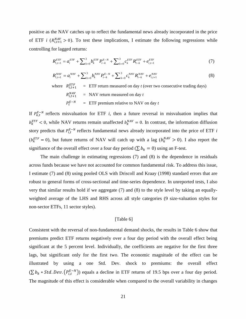
of ETF i (𝑅𝑖,𝑡+1𝑁𝐴𝑉 > 0). To test these implications, I estimate the following regressions while

controlling for lagged returns:

3 3

, 1 , 10 0

ETF ETF ETF E N ETF ETF ETF

i t i k t k k t k i tk kR a b P c R e

(7)

3 3

, 1 , 10 0

NAV NAV NAV E N NAV NAV NAV

i t i k t k k t k i tk kR a b P c R e

(8)

where 𝑅𝑖,𝑡+1𝐸𝑇𝐹

= ETF return measured on day t (over two consecutive trading days)

𝑅𝑖,𝑡+1𝑁𝐴𝑉

= NAV return measured on day t

𝑃𝑡𝐸−𝑁

= ETF premium relative to NAV on day t

If 𝑃𝑘,𝑡𝐸−𝑁 reflects misvaluation for ETF i, then a future reversal in misvaluation implies that

𝑏𝑘𝐸𝑇𝐹 < 0, while NAV returns remain unaffected 𝑏𝑘

𝑁𝐴𝑉 = 0. In contrast, the information diffusion

story predicts that 𝑃𝑖,𝑡𝐸−𝑁 reflects fundamental news already incorporated into the price of ETF i

(𝑏𝑘𝐸𝑇𝐹 = 0), but future returns of NAV will catch up with a lag (𝑏𝑘

𝑁𝐴𝑉 > 0). I also report the

signifiance of the overall effect over a four day period (∑ 𝑏𝑘 = 0) using an F-test.

The main challenge in estimating regressions (7) and (8) is the dependence in residuals

across funds because we have not accounted for common fundamental risk. To address this issue,

I estimate (7) and (8) using pooled OLS with Driscoll and Kraay (1998) standard errors that are

robust to general forms of cross-sectional and time-series dependence. In unreported tests, I also

very that similar results hold if we aggregate (7) and (8) to the style level by taking an equally-

weighted average of the LHS and RHS across all style categories (9 size-valuation styles for

non-sector ETFs, 11 sector styles).

[Table 6]

Consistent with the reversal of non-fundamental demand shocks, the results in Table 6 show that

premiums predict ETF returns negatively over a four day period with the overall effect being

significant at the 5 percent level. Individually, the coefficients are negative for the first three

lags, but significant only for the first two. The economic magnitude of the effect can be

illustrated by using a one Std. Dev. shock to premiums: the overall effect

(∑ 𝑏𝑘 ∗ 𝑆𝑡𝑑. 𝐷𝑒𝑣. (𝑃𝑖,𝑡𝐸−𝑁)) equals a decline in ETF returns of 19.5 bps over a four day period.

The magnitude of this effect is considerable when compared to the overall variability in changes

22

in ETF misvaluation, which is 12 bps per day. In contrast, the overall effect of premiums on

NAV returns over a four day period is insignificantly different from zero.

These results might also be affected by arbitrage activity, namely, from the price impact of

buying the underpriced NAV and selling the overpriced ETF. In order to provide a more

conservative test I investigate the net effect of premiums on future ETF returns relative to NAV

returns (𝑏𝑘𝐸𝑇𝐹 − 𝑏𝑘

𝑁𝐴𝑉). If premiums reflect non-fundamental demand shocks in ETF prices that

subsequently revert, then 𝑏𝑘𝐸𝑇𝐹 − 𝑏𝑘

𝑁𝐴𝑉 < 0, whereas if premiums reflect fundamental demand

shocks in ETF prices and which are subsequently incorporated into NAV prices, then 𝑏𝑘𝐸𝑇𝐹 −

𝑏𝑘𝑁𝐴𝑉 > 0 . Surprisingly, the overall net effect (∑(𝑏𝑘

𝐸𝑇𝐹 − 𝑏𝑘𝑁𝐴𝑉) ∗ 𝑆𝑡𝑑. 𝐷𝑒𝑣. (𝑃𝑖,𝑡

𝐸−𝑁)) is even

more negative than before, at -30.1 bps, because premiums predict NAV returns with a negative

sign on days two and three.

This finding is in contradiction with the information diffusion story predicts, but it can be

explained in the context of non-fundamental demand shocks. Suppose investors trade

sequentially, possibly because information (whether fundamental or non-fundamental) arrives

sequentially. In this case, a positive non-fundamental demand shocks goes first to the most liquid

ETFs. Once liquidity dries up in the most liquid ETF, it goes to the next most liquid and so on,

until no more ETFs are liquid enough relative to their underlying basket, in which case the

demand goes to the underlying securities20

. Thus, a positive premium reflects misvaluation in

both the ETF and the NAV because both are hit by the demand shock, but the ETF is hit harder

because it is more liquid. Consequently, both ETF and NAV prices are above their true

fundamental values, in which case the returns of both must revert.

I also estimate regression (7) and (8) on sub-samples based on non-sector vs. sector, and

for large-, mid- and small-cap funds. The results hold strongly for both non-sector and sector

funds, although among the non-sector funds, only small-cap ETFs show significant evidence of

return reversals following a positive premium. This finding is not only consistent with non-

fundamental demand, but it also agrees with the conjecture that more liquid securities attract

short-term investors with non-fundamental demand because small-cap ETFs have on average

higher relative liquidity compared to either mid- or large-cap ETFs (Broman and Shum, 2015).

20

An alternative explanation is that liquidity demand by retail investors goes first to the most liquid ETF, then to the

next most liquid, and all the way to the least liquid ETF, because trading in the underlying securities is always too

costly. For institutional investors with the capacity to invest in the underlying securities, the demand would go to

ETFs only as long as ETF liquidity is above the liquidity of the underlying securities.

23

7 Correlated demand and excess comovement in returns

The non-fundamentals-based view of excess comovement predicts that if the degree of

commonality in demand shocks varies across securities or over time, then this variation should

be positively related to the degree of commonality in misvaluation and the liquidity of the fund

(Hypothesis 3). In order to test this hypothesis, we need empirical proxies for correlated demand

shocks. In section 7.1, I propose two such measures. In section 7.2 I show that these demand

shock proxies exhibit similar style-based comovements as do changes in ETF misvaluation. In

section 7.3, I provide formal tests for Hypothesis 3.

7.1 Measuring correlated demand shocks

To arrive at a proxy for abnormal demand shocks21

, I build on the concept of abnormal trading

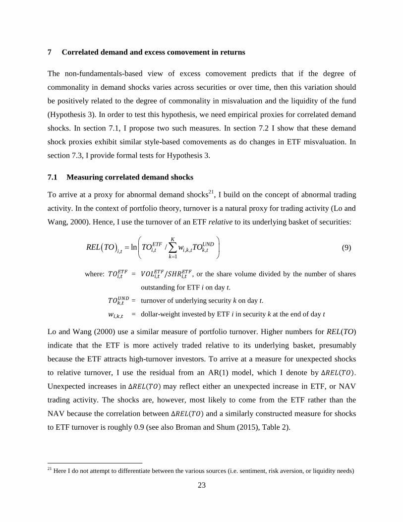
activity. In the context of portfolio theory, turnover is a natural proxy for trading activity (Lo and

Wang, 2000). Hence, I use the turnover of an ETF relative to its underlying basket of securities:

, , , ,,1

ln /K

ETF UNDi t i k t k ti t

k

REL TO TO w TO

(9)

where: 𝑇𝑂𝑖,𝑡𝐸𝑇𝐹 = 𝑉𝑂𝐿𝑖,𝑡

𝐸𝑇𝐹/𝑆𝐻𝑅𝑖,𝑡𝐸𝑇𝐹, or the share volume divided by the number of shares

outstanding for ETF i on day t.

𝑇𝑂𝑘,𝑡𝑈𝑁𝐷 = turnover of underlying security k on day t.

𝑤𝑖,𝑘,𝑡 = dollar-weight invested by ETF i in security k at the end of day t

Lo and Wang (2000) use a similar measure of portfolio turnover. Higher numbers for REL(TO)

indicate that the ETF is more actively traded relative to its underlying basket, presumably

because the ETF attracts high-turnover investors. To arrive at a measure for unexpected shocks

to relative turnover, I use the residual from an AR(1) model, which I denote by ∆𝑅𝐸𝐿(𝑇𝑂).

Unexpected increases in ∆𝑅𝐸𝐿(𝑇𝑂) may reflect either an unexpected increase in ETF, or NAV

trading activity. The shocks are, however, most likely to come from the ETF rather than the

NAV because the correlation between ∆𝑅𝐸𝐿(𝑇𝑂) and a similarly constructed measure for shocks

to ETF turnover is roughly 0.9 (see also Broman and Shum (2015), Table 2).

21

Here I do not attempt to differentiate between the various sources (i.e. sentiment, risk aversion, or liquidity needs)

24

To investigate commonality in relative turnover, I adopt the same approach that I used for

ETF-NAV returns. Specifically, I regress shocks to relative trading activity on the equally-

weighted shock to relative trading activity of other funds in ETF i's own or distant styles (as

defined in the previous section):

1

, , , , ,, , ,1

i i j O i j DI i ti t OWN t j DIST t jj

REL TO REL TO REL TO u

(10)

The one-day leading and lagged terms are meant capture any lagged adjustment in commonality

(Chordia, Roll and Subrahmanyam, 2000). Correlated demand at the style level implies positive

concurrent own-style betas (𝛽𝑖,𝑂). One caveat is that I cannot rule out comovements across styles

(𝛽𝑖,𝐷𝐼 > 0) because ∆𝑅𝐸𝐿(𝑇𝑂) may also capture fundamental demand shocks. Nevertheless, I

would expect to find stronger own- than distant-style comovements if the non-fundamental style

component is strong.

As another measure of correlated demand, I use the degree of commonality in relative

liquidity. There is an extensive literature documenting that liquidity comoves across stocks. The

demand-side view argues that commonality in liquidity arises because of correlated trading

activity (Chordia, Roll and Subrahmanyam, 2000; Karolyi, Lee and Van Dijk, 2012), demand by

institutional owners (Kamara, Lou and Sadka, 2008), by investor sentiment (Huberman and

Halka, 2001) or by the price impact of correlated liquidity needs (Greenwood and Thesmar,

2011). In this case we can view commonality in ETF liquidity as a proxy for correlated demand.

The supply-side view provides a different interpretation. In this case liquidity commonality is

explained by the funding constraints of financial intermediaries. Several theoretical models

predict that commonality in liquidity, via illiquidity spirals or feedback loops, increases during

periods when arbitrage capital is limited22

. However, as we shall see in section 7.2, the results are

more consistent with the demand-side view of liquidity commonality.

To measure relative liquidity, I use the difference between the (log of) Amihud’s price

impact23

for the underlying portfolio and the ETF:

22

see Karolyi, Lee and Van Dijk (2012) for an extensive list of references. 23

Daily observations of the price impact ratio above the 99.5th

percentile of the sample have been discarded as in

Amihud (2002). Similar results obtain if I use the CRSP-based quoted spreads to measure liquidity.

25

, ,

, ,,1 , ,

log /

UND ETFK

k t i t

i k t UND ETFi tk k t i t

R RREL PI w

DVOL DVOL

(11)

where 𝑅𝑖,𝑡𝑈𝑁𝐷 = mid-quite return (in %) for security k held by ETF i, on trading day t

𝐷𝑉𝑂𝐿𝑖,𝑡𝑈𝑁𝐷 = dollar volume (in $millions) for security k, on trading day t

Amihud’s Price Impact (PI) has been widely used in the literature. Hasbrouck (2009) reports

that, “among the daily proxies, the Amihud measure is most strongly correlated with the TAQ-

based price impact coefficient” (p. 1459). Amihud’s measure is also endorsed by several other

papers as good proxy for price impact; others have used it to study commonality in liquidity24

. A

similar measure of portfolio liquidity has been used by Idzorek, Xiong and Ibbotson (2012) and

Broman and Shum (2015). Having defined REL(PI), parallel calculations are done to compute

measures of commonality with REL(TO) replaced by REL(PI) in Eq. (10). The data for portfolio

weights comes from Morningstar Direct25

. For a more detailed description and summary

statistics of these variables, see Broman and Shum (2015).

According to the non-fundamentals based view of excess comovement there is a positive

relationship between the degree of commonality in misvaluation and turnover/liquidity because

both are driven by a common factor, namely correlated demand shocks. It is important to

emphasize that this prediction does not imply that ETF-NAV returns can be explained by relative

turnover/liquidity (or by the own-style turnover/liquidity factors). In particular, commonality in

turnover/liquidity tends to be high during market downturns when volatility is high and when

returns are extremely low (Karolyi, Lee and Van Dijk, 2012), while liquidity is high in the

opposite state and turnover can be high in either extreme state.

The theoretical model by Cherkes, Sagi and Stanton (2008) does, however, predict a

positive relationship between the return difference of twin securities and their liquidity difference

because premiums reflect a trade-off between liquidity and expense ratios. Their prediction can

explain the style-based commonality in misvaluation documented previously only if changes in

relative liquidity are correlated across ETFs at the style level, and if such common changes in

liquidity can explain ETF-NAV return differences. In unreported tests, I investigate this issue by

24

Lesmond (2005), Goyenko, Holden and Trzcinka (2009), Fong, Holden, and Trzcinka (2010) endorse Amihud,

while Karolyi, Lee and Van Dijk (2012) and Kamara, Lou and Sadka (2008) use Amihud for liquidity commonality. 25

Since my holdings data for the underlying holdings of an ETF is generally at the monthly level, the implicit

assumption is that changes in weights only reflect changes in market values of the constituents.

26

regressing changes in premiums (i.e. ETF-NAV returns) on shocks to relative turnover and

relative liquidity (Eq. (9) and (11)) and the own- and distant-style factors for turnover/liquidity.

The liquidity measures are consistently insignificant.

7.2 Results: commonality in demand shocks

Table 7 presents the results for correlated demand shocks, as estimated from Eq. (10) for shocks

to relative turnover (Panel A), or relative liquidity (Panel B). I report the following results:

average and median values for the concurrent, lagged, lead, sum coefficients and R2; the

percentage of funds with positive coefficients, the percentage of funds with positive and

significant coefficients, negative and significant coefficients. Test of statistical significance for

the average (median) coefficient is based on the cross-sectional t-statistic (sign-test) similar to

Chordia, Roll and Subrahmanyam (2000) and Brockman et al. (2009). The results show that

shocks to relative turnover ∆𝑅𝐸𝐿(𝑇𝑂) comove positively and significantly across ETFs in the

same style both at the mean and the median. More than 93 percent of the concurrent own-style

betas (𝛽𝑖,𝑂) are positive and (individually) significant at least at the 5 % level. Although shocks

to relative trading activity also comove across distant styles (𝛽𝑖,𝐷𝐼 > 0), the magnitude of the

distant-style betas are less than a third as large as the own-style betas.

[Table 7]

The results for relative liquidity are even stronger: shocks to relative liquidity exhibit

positive and significant own-style comovements (in 99 percent of cases), while the distant-style

comovements are significantly negative (𝛽𝑖,𝐷𝐼 < 0). This is consistent with the earlier results for

commonality in misvaluation and with the prediction by Barberis and Shleifer (2003) that

increases in own-style allocations are at least partly financed by decreases in distant-style

allocations. Moreover, these style-based comovements in turnover and liquidity are more

consistent with demand than supply-side explanations given that the theoretical effects behind

the latter (illiquidity spirals and feedback loops) are generally described as a market-wide

phenomenon.

Overall, the results in this section highlight that proxies for demand shocks (relative

turnover and price impact) exhibit similar style-based comovements as do ETF-NAV returns.

Similar results are also obtained when turnover/liquidity shocks are measured at the ETF level

27

(ETF turnover or price impact instead of relative turnover or relative price impact), suggesting

that commonality in demand shocks is mainly coming from the ETF, rather than the NAV leg.

7.3 Explaining the amount of commonality in misvaluation

Hypothesis 3 predicts a link between the degree of commonality in misvaluation, commonality in

demand shocks and the level of fund liquidity. In this context, what is the appropriate measure of

the degree of commonality? The existing literature mainly uses the regression R2 (e.g. Morck,

Yeung and Yu, 2000; Hameed, Kang and Viswanathan, 2010; Karolyi, Lee and Van Dijk, 2012),

although the beta coefficient is also used (Kamara, Lou and Sadka, 2008).

I use the R2 measure for three reasons. First, the beta is sensitive to scaling effects that arise

from differences in factors and their volatilities (i.e. the beta denominator) across ETF styles.

Second, it is difficult to make cross-sectional comparisons of betas in short samples due to large

cross-sectional differences in the Std. Dev. of ETF-NAV returns, which is also directly related to

arbitrage costs (funds with higher arbitrage costs have more volatile ETF-NAV returns). The R2-

measure does not suffer from these problems as it is a function of both the variance of the

dependent variable and the factors. Another interpretation of the R2-measure is that it captures

the proportion of common vs. idiosyncratic risk, in which case it is not sensitive to total

misvaluation. This metric is also suitable for testing the hypothesis that commonality in

misvaluation is stronger for more liquid ETFs. In unreported robustness tests I verify that the

main results continue to hold for beta coefficients.

The regression R2 (labelled 𝑅𝑟𝑒𝑡,𝑚

2 ) from Eq. (4) is estimated every month m on daily data.

I require at least 15 non-missing observations per month. Since regression (4) also controls for

the lagged premium, I decompose the model R2 as:

, , 1 , , , ,, ,

, , ,

, , ,2E N E N E N E N E N E N

ii t i t i t OWN t i t DI ti OWN i DI

E N E N E Ni t i t i t

COV R P COV R R COV R R

mVAR R VAR R VAR R

R

(12)

and use the sum of the last two normalized covariance terms, denoted 𝑅𝑟𝑒𝑡,𝑚2 , to measure the

degree of commonality in misvaluation. 𝑅𝑟𝑒𝑡,𝑚2 can be interpreted as the fraction of the model R

2

attributable to the own- and distant-style factors (Graham, Li and Qiu, 2013). Similarly, I

measure commonality in relative turnover/liquidity shocks from the fraction of model R2

28

attributable to the concurrent own and distant-style factors from Eq. (10). The degree of

commonality in relative turnover and price impact is denoted by 𝑅𝑟𝑇𝑂,𝑚2 and 𝑅𝑟𝑃𝐼,𝑚

2 respectively.

To investigate the relationship between commonality in misvaluation, commonality in

demand shocks and liquidity, I estimate the following regression using pooled OLS:

2 2

, 1 , 1 2 , 1 3 , 1 4 ,ret m dem m i m i m m i mR a b R b LIQ b Fund b Macro FE e (13)

where 𝑅𝑑𝑒𝑚,𝑚−12 = commonality in demand shocks based on 𝑅𝑟𝑇𝑂,𝑚

2 or 𝑅𝑟𝑃𝐼,𝑚2

𝐿𝐼𝑄𝑖,𝑡−1 = ETF & underlying portfolio liquidity during month t-1

𝐹𝑢𝑛𝑑𝑖,𝑚−1 = vector of fund characteristics

𝑀𝑎𝑐𝑟𝑜𝑚 = vector of macro variables

𝐹𝐸 = fixed effects: year, month, sector, style and/or fund

As a direct and salient measure of liquidity, I use the monthly average quoted spread for ETF i:

, ,,

1 , ,

11*ln 100*

/ 2

mETF ETFNi t i tETF

i m ETF ETFm t i t i t

ASK BIDQSPR

N ASK BID

(14)

where: 𝐴𝑆𝐾𝑖,𝑡𝐸𝑇𝐹and 𝐵𝐼𝐷𝑖,𝑡

𝐸𝑇𝐹 = CRSP ask and bid price at the close on trading day t for ETF i

Nm = nr. of trading days in calendar month m

I use the log-transformation to mitigate the impact of outliers and to deal with the apparent non-

stationarity in the data. I estimate the portfolio quoted spread by dollar-weighting the monthly

quoted spread of each security included in the ETF’s basket ( 𝑄𝑆𝑃𝑅𝑖,𝑚𝑈𝑁𝐷 = 𝑤𝑖,𝑘,𝑚𝑄𝑆𝑃𝑅𝑘,𝑚

𝑈𝑁𝐷 ).

According to Chung and Zhang (2014), the CRSP-based spread is highly correlated with the

(more accurate) TAQ spread in the cross-section, which is the dimension of primary interest. I

also include the expense ratio because it is a salient cost for retail investors (Grinblatt et al.,

2014). Another implicit measure of liquidity is total misvaluation, measured by the absolute

value of the monthly average premium (Eq. (2)), because funds with high misvaluation have high

arbitrage costs.

Arbitrage activity should be negatively related to the degree of commonality in

misvaluation because it is associated with greater pricing efficiency. To measure arbitrage

activity, I use share creation/redemption activity, defined as in Broman and Shum (2015):

29

, , 1

,

1 , 1

1log 1

Nmi d i d

i m

dm i d

SHR SHRCREATE

N SHR

(15)

where: 𝑆𝐻𝑅𝑖,𝑑 = shares outstanding for ETF i on day d;

Nt = number of trading days in calendar month t.

Commonality in misvaluation should be greater when market-wide arbitrage costs are high

because they leave more “room” for excess comovement (Kumar and Lee, 2006; Kumar and

Spalt, 2013). I use the funding liquidity factor by Hu, Pan and Wang (2013), which is based on

price deviations between on-the-run and off-the-run Treasury securities, averaged across a wide

range of maturities. Market volatility is also an important determinant of the risk to market

makers of maintaining inventories of their securities (Chordia, Roll, and Subrahmanyam, 2000),

and changes in market volatility can cause changes in inventories and create correlated

institutional trading. Market volatility is also related aggregate uncertainty in financial markets

either via higher transaction costs or lower funding liquidity (i.e., less capital is devoted to ETF

arbitrage) as in Brunnermeier and Pedersen (2009). In either case, the prediction is that

commonality in misvaluation should be positively related to market volatility, which I proxy for

by the Std. Dev. of NAV returns.

[Figure 1]

Before I discuss the regression results, I illustrate the time-series dynamics for the cross-

sectional mean degree of commonality in misvaluation (𝑅𝑟𝑒𝑡,𝑚2 ) in Figure 1. Panel A depicts

𝑅𝑟𝑒𝑡,𝑚2 across three terciles based on the degree of commonality in relative liquidity (via price

impact) in the prior month (𝑅𝑟𝑃𝐼,𝑚−12 ), while in Panel B, I instead use three terciles based on

relative quoted spreads (𝑄𝑆𝑃𝑅𝑖,𝑚−1𝐸𝑇𝐹 − 𝑄𝑆𝑃𝑅𝑖,𝑚−1

𝑈𝑁𝐷 ). We can see that ETFs in the top tercile of

commonality in relative price impact have a higher degree of commonality in misvaluation in 99

% of quarters (93 % are significant at the 5 % level) relative to ETFs in the lowest tercile.

Moreover, ETFs in the highest tercile of relative quoted spreads have stronger commonality in

misvaluation in 98 % of the quarters (70 % are significant at the 5 % level). These preliminary

findings agree with the conjecture that commonality in misvaluation is higher when commonality

in demand shocks is high, and for ETFs with more desirable liquidity characteristics.

[Table 8]

30

The results in Table 8 show that commonality in misvaluation is positively and

significantly related to commonality in demand shocks (via 𝑅𝑟𝑇𝑂2 and 𝑅𝑟𝑃𝐼

2 ). When both measures

for commonality in demand shocks are included simulatenously, 𝑅𝑟𝑃𝐼2 remains highly significant

while 𝑅𝑟𝑇𝑂2 is only marginally significant. This is not surprising because the two measures are

designed to capture the same thing. Moreover, commonality in misvaluation is significantly

higher for more liquid ETFs (lower quoted spreads, expense ratios and total misvaluation), for

less liquid underlying portfolios, and during times when arbitrage is limited (high market

volatility, low funding liquidity). Similar results are obtained in sub-samples of non-sector vs.

sector funds, or if we control for time or ETF fixed effects in addition to style fixed effects.

Overall, the findings in this section show that the degree of commonality in misvaluation is

stronger for ETFs with more correlated demand shocks and more desirable liquidity

characteristics, which supports my conjecture that excess comovements in ETF returns are

driven by correlated non-fundamental demand and facilitated by investors with short horizons

that are attracted to ETFs because of their high liquidity.

8 Summary and Conclusions

This study analyzes whether the returns of Exchange Traded Funds (ETFs) comove excessively

with other ETFs in similar investment styles. My conjecture is that, due to the ease of investing

in ETFs and because of their high liquidity, ETFs attract a clientele of short-term investors who

are more exposed to common non-fundamental demand shocks at the style level relative to the

investor in the ETFs underlying baskets.

In order to identify excess comovements, I look for common factors in changes in

misvaluation (ETF-NAV returns); in order to attribute this misvaluation to the ETF leg, I study

return reversals following shocks to misvaluation; and in order to link the degree of excess

comovement to common non-fundamental demand shocks and to liquidity clientele differences, I

investigate how the degree of commonality in misvaluation is related to the degree of

commonality in turnover/liquidity (proxy for demand shocks) and ETF characteristics that are

attractive to investors with short-term trading needs.

My findings indicate that there is significant style-based commonality in misvaluation:

changes in misvaluation comove positively across ETFs in similar styles, and negatively with

ETFs in distant styles. Although the importance of common misvaluation is found to persist

31

across daily, weekly and monthly horizons, the economic magnitude of these shocks declines

with the return horizon consistent with arbitrage. The source of misvaluation is found to be the

ETF since current ETF premiums negatively predict future ETF returns consistent with

temporary demand shocks in the ETF prices. Such reversals are strongest for small-cap ETFs,

which is consistent with the conjecture that more liquid securities (small-cap ETFs have the

highest relative liquidity) attract short-term investors with non-fundamental demand.

Moreover, shocks to the abnormal trading activity of ETFs and to the liquidity of ETFs

(both relative to their underlying baskets) exhibit similar style-based commonality. These proxies

for correlated demand shocks also predict the future amount of commonality in ETF

misvaluation. In accordance with liquidity being a factor in inducing clientele differences

between ETFs and their underlying portfolio, I show that the degree of commonality in

misvaluation is higher among ETFs more desirable liquidity characteristics.

My overall conclusion is that the excess comovement in ETF returns is mainly driven by

the correlated non-fundamental demand of a liquidity-based clientele. Thus, more liquid

securities may encourage trading for reasons unrelated to fundamentals, which can at times be

detrimental for pricing efficiency.

References

Aggarwal, R. and Schofield, L. (2012): The Growth of Global ETFs and Regulatory Challenges. Available at

SSRN: http://ssrn.com/abstract=2001060 or http://dx.doi.org/10.2139/ssrn.2001060

Amihud, Y., & Mendelson, H. (1986). Asset pricing and the bid-ask spread. Journal of financial Economics, 17(2),

223-249.

Amihud, Y. (2002). Illiquidity and stock returns: cross-section and time-series effects. Journal of financial markets,

5(1), 31-56.

Anton, M., & Polk, C. (2014). Connected stocks. The Journal of Finance, 69 (3), pp. 1099-1127.

Baker, M., & Wurgler, J. (2006). Investor Sentiment and the Cross-Section of Stock Returns. The Journal of

Finance, 61(4), 1645-1680.

Banz, R. W. (1981). The relationship between return and market value of common stocks. Journal of financial

economics, 9(1), 3-18.

Barber, B. M., Odean, T., & Zhu, N. (2009). Do retail trades move markets?. Review of Financial Studies, 22(1),

151-186.

Barberis, N., & Shleifer, A. (2003). Style investing. Journal of Financial Economics, 68(2), 161-199.

Barberis, N., Shleifer, A., & Wurgler, J. (2005). Comovement. Journal of Financial Economics, 75(2), 283-317.

32

Barberis, N., & Thaler, R. (2003). A survey of behavioral finance. Handbook of the Economics of Finance, 1, 1053-

1128.

Ben-David, I., Franzoni, F., and Moussawi, R. (2014): Do ETFs Increase Volatility? Available at SSRN:

http://ssrn.com/abstract=1967599.

Ben-Rephael, A., Kadan, O., and Wohl, A. (2013): The Diminishing Liquidity Premium. Journal of Financial and

Quantitative Analysis, Forthcoming.

Blackrock (2012): ETP Landscape, Global handbook 2012. Availble at:

http://www.blackrockinternational.com/intermediaries/en-fi/insights/etp-landscape

Bodurtha, J.N., Kim, D-S., Lee, C.M.C (1995): Closed-end Country Funds and U.S. Market Sentiment, The Review

of Financial Studies, Vol. 8, No. 3, pp. 879-918.

Brav, A., Heaton, J. B., & Li, S. (2010). The limits of the limits of arbitrage. Review of Finance, 14(1), 157-187.

Brockman, P., Chung, D. Y., & Pérignon, C. (2009). Commonality in liquidity: A global perspective. Journal of

Financial and Quantitative Analysis, 44(04), 851-882.

Brown, S. J., & Goetzmann, W. N. (1997). Mutual fund styles. Journal of financial Economics, 43(3), 373-399.

Broman, M. and Shum, P. (2015): Short-Term Trading and Liquidity Clienteles: Evidence from Exchange-Traded

Funds. Available at http://papers.ssrn.com/sol3/papers.cfm?abstract_id=2361514

Campbell, J. Y., Polk, C., & Vuolteenaho, T. (2010). Growth or glamour? Fundamentals and systematic risk in stock

returns. Review of Financial Studies, 23(1), 305-344.

Campbell, J. Y., Giglio, S., Polk, C., & Turley, R. (2013). An Intertemporal CAPM with Stochastic Volatility (No.

w18411). National Bureau of Economic Research.

Chan, L. K., Chen, H. L., & Lakonishok, J. (2002). On mutual fund investment styles. Review of financial studies,

15(5), 1407-1437.

Chan, J. S., Hong, D., & Subrahmanyam, M. G. (2008). A tale of two prices: Liquidity and asset prices in multiple

markets. Journal of Banking & Finance, 32(6), 947-960.

Cherkes, M., Sagi, J., & Stanton, R. (2009). A liquidity-based theory of closed-end funds. Review of Financial

Studies, 22(1), 257-297.

Chordia, T., Roll, R., & Subrahmanyam, A. (2000). Commonality in liquidity. Journal of Financial Economics,

56(1), 3-28.

Cooper, M. J., Gulen, H., & Rau, P. R. (2005). Changing names with style: Mutual fund name changes and their

effects on fund flows. The Journal of Finance, 60(6), 2825-2858.

Da, Z., & Shive, S. (2013). When the Bellwether Dances to Noise: Evidence from Exchange-Traded Funds.

Available at SSRN: http://ssrn.com/abstract=2158361.

DeLisle, Jared and French, Dan W. and Schutte, Maria G. (2013): What Does Rising Comovement Mean for Price

Informativeness? An Examination of Average R2 Trends). Available at SSRN:

http://ssrn.com/abstract=2166118

DeLong, J. B., Shleifer, A., Summers, L.H. and Waldmann, R. (1990): Noise trader risk in financial markets.

Journal of Political Economy, 98(4):703-738.

Driscoll, John C., and Aart C. Kraay (1998): Consistent covariance matrix estimation with spatially dependent panel

data, Review of Economics and Statistics 80, pp. 549–560.

33

Engle, R. and Sarkar, D. (2006): Premiums-Discounts and Exchange Traded Funds. The Journal of Derivatives,

2006 (1), pp. 27-45.

Fama, Eugene F., and Kenneth R. French, 1993, Common risk factors in the returns on stocks and bonds, Journal of

Financial Economics 33, 3–56.

Fama, Eugene F., and Kenneth R. French, 1995, Size and book-to-market factors in earnings and returns, Journal of

Finance, 50, 131–155.

Frazzini, A., & Lamont, O. A. (2008). Dumb money: Mutual fund flows and the cross-section of stock returns.

Journal of Financial Economics, 88(2), 299-322.

Fong, K., Holden, C.W., Trzcinka, C.A. (2010): Can global stock liquidity be measured? Unpublished working

paper. University of New South Wales and Indiana University.

Froot, K., & Teo, M. (2008). Style investing and institutional investors. Journal of Financial and Quantitative

Analysis, 43(4), 883.

Gagnon, L., & Andrew Karolyi, G. (2010). Multi-market trading and arbitrage. Journal of Financial Economics,

97(1), 53-80.

Graham, J. R., Li, S., & Qiu, J. (2012). Managerial attributes and executive compensation. Review of Financial

Studies, 25(1), 144-186.

Green, T. C., & Hwang, B. H. (2009). Price-based return comovement. Journal of Financial Economics, 93(1), 37-

50.

Greenwich Associates (2013): Institutional Investors Relation with ETFs deepen. Available at:

http://us.ishares.com/content/en_us/repository/resource/greenwich_survey_inst.pdf

Greenwood, R. (2007): Excess comovement of stock returns: Evidence from cross-sectional variation in Nikkei 225

weights. Review of Financial Studies, 21.3, pp. 1153-1186.

Greenwood, R., & Thesmar, D. (2011). Stock price fragility. Journal of Financial Economics, 102(3), 471-490.

Goyenko, R. Y., Holden, C. W., & Trzcinka, C. A. (2009). Do liquidity measures measure liquidity? Journal of

Financial Economics, 92(2), 153-181.

Hardouvelis, G., Porta, R. L., & Wizman, T. A. (1994). What moves the discount on country equity funds?. In The

internationalization of equity markets (pp. 345-403). University of Chicago Press.

Hameed, A., Kang, W., & Viswanathan, S. (2010). Stock market declines and liquidity. The Journal of Finance,

65(1), 257-293.

Hasbrouck, J. (2009). Trading costs and returns for US equities: Estimating effective costs from daily data. The

Journal of Finance, 64(3), 1445-1477.

Huang, M. (2003). Liquidity shocks and equilibrium liquidity premia. Journal of Economic Theory, 109(1), 104-

129.

Hu, G. X., Pan, J., & Wang, J. (2013). Noise as information for illiquidity. The Journal of Finance, 68(6), 2341-

2382.

Huberman, G., Halka, D. (2001): Systematic liquidity. Journal of Financial Research, 24,pp. 161–178.

Idzorek, T. M, Xiong, J. X. and Ibbotson, R. G. (2012). The Liquidity Style of Mutual Funds. Financial Analyst

Journal, 68 (6),

34

Kamara, A., Lou, X., & Sadka, R. (2008). The divergence of liquidity commonality in the cross-section of stocks.

Journal of Financial Economics, 89(3), 444-466.

Karolyi, G. A., Lee, K. H., & Van Dijk, M. A. (2012). Understanding commonality in liquidity around the world.

Journal of Financial Economics, 105(1), 82-112.

Kasch, M., & Sarkar, A. (2012). Is there an S&P 500 Index effect?. Available at SSRN 2171235.

Korajczyk, R. A., & Sadka, R. (2008). Pricing the commonality across alternative measures of liquidity. Journal of

Financial Economics, 87(1), 45-72.

Kumar, A., & Lee, C. (2006). Retail investor sentiment and return comovements. The Journal of Finance, 61(5),

2451-2486.

Kumar, A. (2009). Dynamic style preferences of individual investors and stock returns. Journal of Financial and

Quantitative Analysis, 44(03), 607-640.

Kumar, A., Page, J. K., & Spalt, O. G. (2013). Investor Sentiment and Return Comovements: Evidence from Stock

Splits and Headquarters Changes. Review of Finance, 17(3), 921-953.

Kumar, A., Page, J. K., & Spalt, O. G. (2013b): Gambling and Comovement. Journal of Financial and Quantitative

Analysis, forthcoming.

Lee, C.M., Shleifer, A. and Thaler, R.H. (1991): Investor Sentiment and the Closed-End Fund Puzzle. The Journal

of Finance, XLVI (1), pp. 75-109.

Lesmond, D. (2005): Liquidity of emerging markets. Journal of Financial Economics, 77, 411–452.

Lo, A. W., & Wang, J. (2000). Trading volume: definitions, data analysis, and implications of portfolio theory.

Review of Financial Studies, 13(2), 257-300.

Lo, A., W., Mamaysky, H., & Wang, J. (2004). Asset Prices and Trading Volume under Fixed Transactions Costs.

Journal of Political Economy, 112(5).

Lynch, A. W., & Tan, S. (2011). Explaining the Magnitude of Liquidity Premia: The Roles of Return Predictability,

Wealth Shocks, and State-Dependent Transaction Costs. The Journal of Finance, 66(4), 1329-1368.

Marshall, B. R., Nguyen, N. H., & Visaltanachoti, N. (2013). ETF arbitrage: Intraday Evidence. Journal of Banking

and Finance, 37(9), 3486-3498.

Merton, R. C. (1973). An intertemporal capital asset pricing model. Econometrica: Journal of the Econometric

Society, 867-887.

Morck, R., Yeung, B., & Yu, W. (2000): The information content of stock markets: why do emerging markets have

synchronous stock price movements?. Journal of financial economics, 58(1), 215-260.

Perez, F., Shkilko, A., & Tang, T. (2011): Signaling Via Stock Splits: Evidence from Short Interest. In AFA 2012

Chicago Meetings Paper.

Petajisto, A (2013): Inefficiencies in the Pricing of Exchange-Traded Funds. Available at SSRN:

http://ssrn.com/abstract=2000336 or http://dx.doi.org/10.2139/ssrn.1572907

Pontiff, J. (2006). Costly arbitrage and the myth of idiosyncratic risk. Journal of Accounting and Economics, 42(1),

35-52.

Pirinsky, C., & Wang, Q. (2006). Does corporate headquarters location matter for stock returns? The Journal of

Finance, 61(4), 1991-2015.

35

Richie, Nivine, Robert Daigler, and Kimberly C. Gleason (2008): The limits to stock index arbitrage: Examining

S&P 500 futures and SPDRs, Journal of Futures Markets, 28(12), 1182– 1205.

Rinne, K., Suominen, M., & Vaittinen, L. (2014). Dash for Cash: Month-End Liquidity Needs and the Predictability

of Stock Returns. Available at SSRN.

Staer, A. (2014). Fund Flows and Underlying Returns: The Case of ETFs. Available at SSRN 2158468.

Teo, M., & Woo, S. J. (2004). Style effects in the cross-section of stock returns. Journal of Financial Economics,

74(2), 367-398.

Wurgler, Jeffrey (2010): On the Economic Consequences of Index-Linked Investing, National Bureau of Economic

Research Working Paper Series No. 16376.

Yan, X. S. (2008). Liquidity, investment style, and the relation between fund size and fund performance. Journal of

Financial and Quantitative Analysis, 43(03), 741-767.

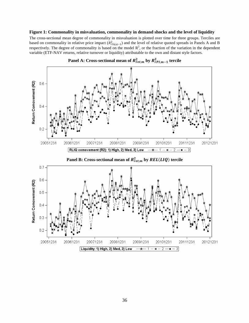
36

Figure 1: Commonality in misvaluation, commonality in demand shocks and the level of liquidity

The cross-sectional mean degree of commonality in misvaluation is plotted over time for three groups. Terciles are

based on commonality in relative price impact (𝑅𝑟𝑙𝑖𝑞,𝑞−12 ) and the level of relative quoted spreads in Panels A and B

respectively. The degree of commonality is based on the model R2, or the fraction of the variation in the dependent

variable (ETF-NAV returns, relative turnover or liquidity) attributable to the own and distant style factors.

Panel A: Cross-sectional mean of 𝑹𝒓𝒆𝒕,𝒎𝟐 by 𝑹𝒓𝑷𝑰,𝒎−𝟏

𝟐 tercile

Panel B: Cross-sectional mean of 𝑹𝒓𝒆𝒕,𝒎𝟐 by 𝑹𝑬𝑳(𝑳𝑰𝑸) tercile

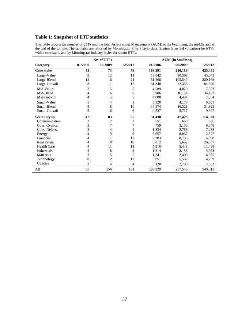
37

Table 1: Snapshot of ETF statistics

This table reports the number of ETFs and the total Assets under Management (AUM) at the beginning, the middle and at

the end of the sample. The statistics are reported by Morningstar 3-by-3 style classification (size and valuation) for ETFs

with a core style, and by Morningstar industry styles for sector ETFs.

Nr. of ETFs AUM (in $millions)

Category 01/2006 06/2009 12/2012 01/2006 06/2009 12/2012

Core styles 53 73 79 168,391 210,116 425,491

Large-Value 8 12 11 16,042 20,398 43,041

Large-Blend 12 16 21 81,368 105,540 220,168 Large-Growth 8 11 12 31,840 33,355 64,670

Mid-Value 3 5 5 4,589 4,020 7,373

Mid-Blend 4 6 6 6,906 16,174 34,492 Mid-Growth 4 5 5 4,008 4,404 7,854

Small-Value 5 4 3 5,228 4,178 6,661

Small-Blend 4 8 10 13,874 16,321 31,925

Small-Growth 5 6 6 4,537 5,727 9,307

Sector styles 42 83 85 31,438 47,428 114,520

Communication 2 2 2 551 650 936

Cons. Cyclical 3 7 7 759 3,158 9,348

Cons. Defens. 3 4 4 1,334 2,756 7,258

Energy 4 9 9 6,657 8,067 12,877

Financial 4 11 13 2,383 8,756 14,098

Real Estate 4 10 10 5,012 5,652 26,087

Health Care 4 11 11 5,216 5,448 11,498

Industrials 4 8 8 1,314 2,188 5,953

Materials 3 5 5 1,241 2,406 4,675

Technology 8 12 12 3,851 5,562 14,239 Utilities 3 4 4 3,120 2,788 7,552

All 95 156 164 199,829 257,545 540,011

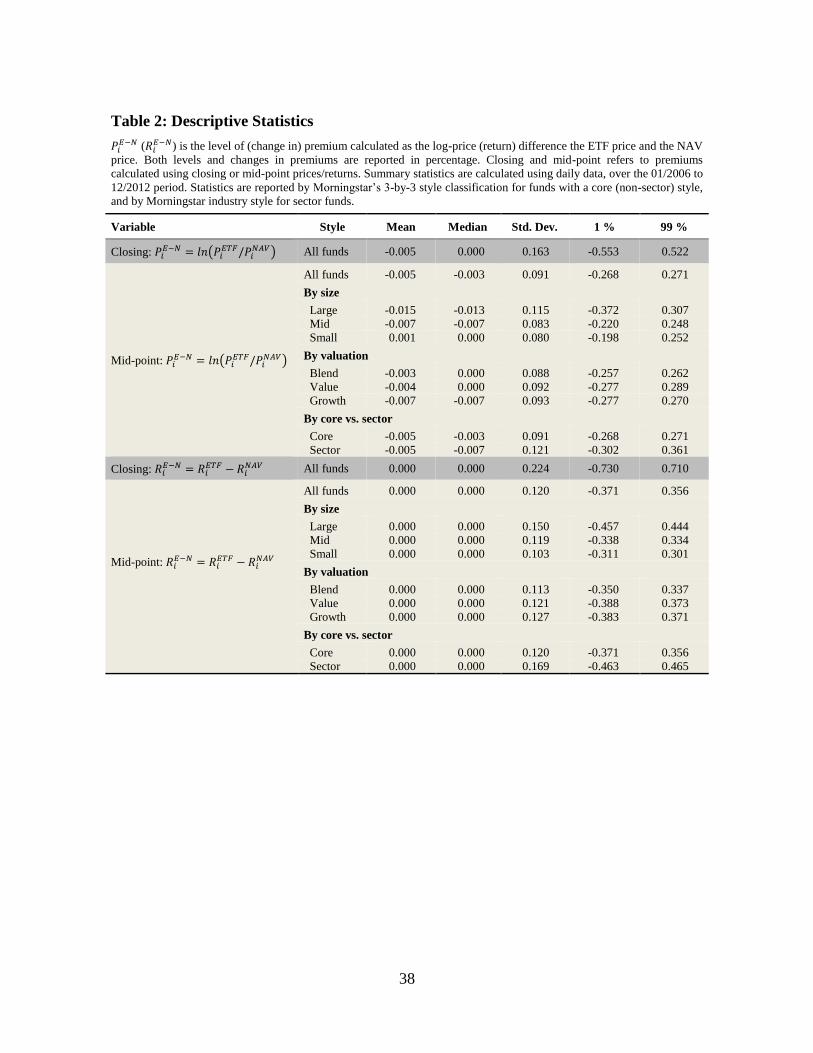
38

Table 2: Descriptive Statistics

𝑃𝑖𝐸−𝑁 (𝑅𝑖

𝐸−𝑁) is the level of (change in) premium calculated as the log-price (return) difference the ETF price and the NAV

price. Both levels and changes in premiums are reported in percentage. Closing and mid-point refers to premiums

calculated using closing or mid-point prices/returns. Summary statistics are calculated using daily data, over the 01/2006 to

12/2012 period. Statistics are reported by Morningstar’s 3-by-3 style classification for funds with a core (non-sector) style,

and by Morningstar industry style for sector funds.

Variable Style Mean Median Std. Dev. 1 % 99 %

Closing: 𝑃𝑖𝐸−𝑁 = 𝑙𝑛(𝑃𝑖

𝐸𝑇𝐹/𝑃𝑖𝑁𝐴𝑉) All funds -0.005 0.000 0.163 -0.553 0.522

Mid-point: 𝑃𝑖𝐸−𝑁 = 𝑙𝑛(𝑃𝑖

𝐸𝑇𝐹/𝑃𝑖𝑁𝐴𝑉)

All funds -0.005 -0.003 0.091 -0.268 0.271

By size

Large -0.015 -0.013 0.115 -0.372 0.307

Mid -0.007 -0.007 0.083 -0.220 0.248

Small 0.001 0.000 0.080 -0.198 0.252

By valuation

Blend -0.003 0.000 0.088 -0.257 0.262

Value -0.004 0.000 0.092 -0.277 0.289

Growth -0.007 -0.007 0.093 -0.277 0.270

By core vs. sector

Core -0.005 -0.003 0.091 -0.268 0.271

Sector -0.005 -0.007 0.121 -0.302 0.361

Closing: 𝑅𝑖𝐸−𝑁 = 𝑅𝑖

𝐸𝑇𝐹 − 𝑅𝑖𝑁𝐴𝑉 All funds 0.000 0.000 0.224 -0.730 0.710

Mid-point: 𝑅𝑖𝐸−𝑁 = 𝑅𝑖

𝐸𝑇𝐹 − 𝑅𝑖𝑁𝐴𝑉

All funds 0.000 0.000 0.120 -0.371 0.356

By size

Large 0.000 0.000 0.150 -0.457 0.444

Mid 0.000 0.000 0.119 -0.338 0.334

Small 0.000 0.000 0.103 -0.311 0.301

By valuation

Blend 0.000 0.000 0.113 -0.350 0.337

Value 0.000 0.000 0.121 -0.388 0.373

Growth 0.000 0.000 0.127 -0.383 0.371

By core vs. sector

Core 0.000 0.000 0.120 -0.371 0.356

Sector 0.000 0.000 0.169 -0.463 0.465

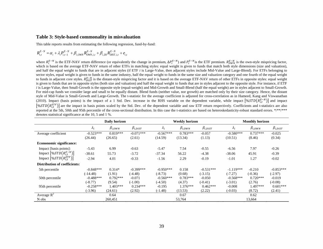
39

Table 3: Style-based commonality in misvaluation

This table reports results from estimating the following regression, fund-by-fund:

, , 1 , , , , , , ,

E N E N E N E N

i t i i i t i OWN OWN i t i DI DIST i t i tR P R R e

where 𝑅𝑖𝐸−𝑁 is the ETF-NAV return difference (or equivalently the change in premium, ∆𝑃𝑖

𝐸−𝑁) and 𝑃𝑖𝐸−𝑁is the ETF premium. 𝑅𝑂𝑊𝑁

𝐸−𝑁 is the own-style mispricing factor,

which is based on the average ETF-NAV return of other ETFs in matching styles: equal weight is given to funds that match both style dimensions (size and valuation),

and half the equal weight to funds that are in adjacent styles (if ETF i is Large-Value, then adjacent styles include Mid-Value and Large-Blend). For ETFs belonging to

sector styles, equal weight is given to funds in the same industry, half the equal weight to funds in the same size and valuation category and one fourth of the equal weight

to funds in adjacent core styles. 𝑅𝐷𝐼𝑆𝑇𝐸−𝑁 is the distant-style mispricing factor and it is based on the average ETF-NAV return of other ETFs in opposite styles: equal weight

is given to funds that are in opposite styles (both size and valuation) and half the equal weight to funds that are in styles adjacent to the opposite style. For instance, if ETF

i is Large-Value, then Small-Growth is the opposite style (equal-weight) and Mid-Growth and Small-Blend (half the equal weight) are in styles adjacent to Small-Growth.

For mid-cap funds we consider large and small to be equally distant. Blend funds (neither value, nor growth) are matched only by their size category. Hence, the distant

style of Mid-Value is Small-Growth and Large-Growth. The t-statistic for the average coefficient is adjusted for cross-correlation as in Hameed, Kang and Viswanathan

(2010). Impact (basis points) is the impact of a 1 Std. Dev. increase in the RHS variable on the dependent variable, while impact [%𝑆𝑇𝐷(𝑅𝑖,𝑡𝐸−𝑁)] and impact

[%𝑆𝑇𝐷(𝑅𝑖,𝑡𝐸𝑇𝐹)] are the impact in basis points scaled by the Std. Dev. of the dependent variable and raw ETF return respectively. Coefficients and t-statistics are also

reported at the 5th, 50th and 95th percentile of the cross-sectional distribution. In this case the t-statistics are based on heteroskedasticity-robust standard errors. */**/***

denotes statistical significance at the 10, 5 and 1 %.

Daily horizon Weekly horizon Monthly horizon

𝜆𝑖 𝛽𝑖,𝑂𝑊𝑁 𝛽𝑖,𝐷𝐼𝑆𝑇 𝜆𝑖 𝛽𝑖,𝑂𝑊𝑁 𝛽𝑖,𝐷𝐼𝑆𝑇 𝜆𝑖 𝛽𝑖,𝑂𝑊𝑁 𝛽𝑖,𝐷𝐼𝑆𝑇

Average coefficient -0.523*** 0.819*** -0.071*** -0.567*** 0.783*** -0.057 -0.580*** 0.737*** -0.025

(26.44) (26.65) (2.61) (14.59) (13.34) (1.13) (10.51) (8.46) (0.34)

Econonomic significance:

Impact [basis points]: -5.43 6.99 -0.63 -5.47 7.54 -0.55 -6.56 7.97 -0.26

Impact [%𝑆𝑇𝐷(𝑅𝑖,𝑡𝐸−𝑁)] -38.61 55.73 -3.72 -37.34 56.22 -4.38 -38.06 45.91 -0.39

Impact [%𝑆𝑇𝐷(𝑅𝑖,𝑡𝐸𝑇𝐹)] -2.94 4.01 -0.33 -1.56 2.29 -0.19 -1.01 1.27 -0.02

Distribution of coefficients:

5th percentile -0.848*** 0.314* -0.399*** -0.950*** 0.158 -0.531*** -1.119*** -0.210 -0.853***

(-14.48) (1.91) (-4.48) (-8.73) (0.68) (-3.15) (-7.27) (-0.36) (-2.97)

50th percentile -0.488*** 0.792*** -0.071 -0.560*** 0.783*** -0.050 -0.568*** 0.720*** -0.019

(-8.77) (9.54) (-1.00) (-4.50) (4.37) (-0.41) (-3.01) (2.76) (-0.08)

95th percentile -0.258*** 1.403*** 0.234*** -0.195 1.376*** 0.462*** -0.008 1.497*** 0.601***

(-3.96) (24.61) (2.92) (-1.48) (13.53) (2.22) (-0.03) (8.72) (2.41)

Average R2 0.64 0.67 0.62

N obs 260,451 53,764 13,664

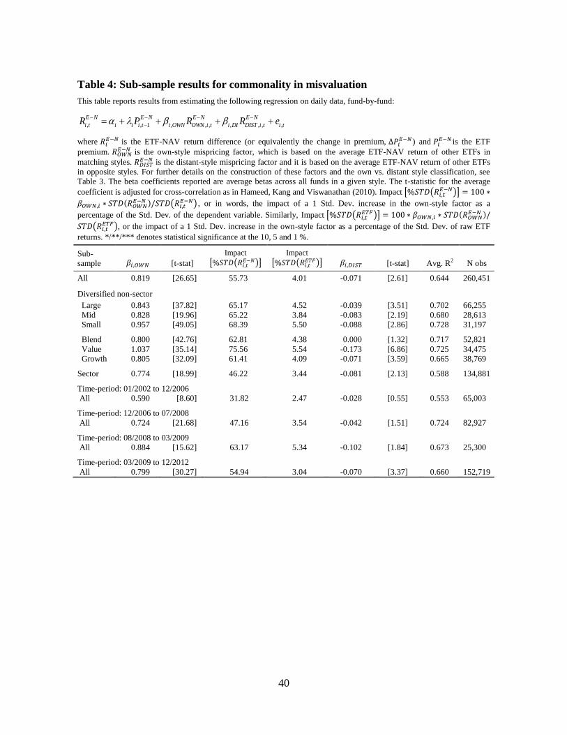
40

Table 4: Sub-sample results for commonality in misvaluation

This table reports results from estimating the following regression on daily data, fund-by-fund:

, , 1 , , , , , , ,

E N E N E N E N

i t i i i t i OWN OWN i t i DI DIST i t i tR P R R e

where 𝑅𝑖𝐸−𝑁 is the ETF-NAV return difference (or equivalently the change in premium, ∆𝑃𝑖

𝐸−𝑁) and 𝑃𝑖𝐸−𝑁 is the ETF

premium. 𝑅𝑂𝑊𝑁𝐸−𝑁 is the own-style mispricing factor, which is based on the average ETF-NAV return of other ETFs in

matching styles. 𝑅𝐷𝐼𝑆𝑇𝐸−𝑁 is the distant-style mispricing factor and it is based on the average ETF-NAV return of other ETFs

in opposite styles. For further details on the construction of these factors and the own vs. distant style classification, see

Table 3. The beta coefficients reported are average betas across all funds in a given style. The t-statistic for the average

coefficient is adjusted for cross-correlation as in Hameed, Kang and Viswanathan (2010). Impact [%𝑆𝑇𝐷(𝑅𝑖,𝑡𝐸−𝑁)] = 100 ∗

𝛽𝑂𝑊𝑁,𝑖 ∗ 𝑆𝑇𝐷(𝑅𝑂𝑊𝑁𝐸−𝑁 )/𝑆𝑇𝐷(𝑅𝑖,𝑡

𝐸−𝑁) , or in words, the impact of a 1 Std. Dev. increase in the own-style factor as a

percentage of the Std. Dev. of the dependent variable. Similarly, Impact [%𝑆𝑇𝐷(𝑅𝑖,𝑡𝐸𝑇𝐹)] = 100 ∗ 𝛽𝑂𝑊𝑁,𝑖 ∗ 𝑆𝑇𝐷(𝑅𝑂𝑊𝑁

𝐸−𝑁 )/

𝑆𝑇𝐷(𝑅𝑖,𝑡𝐸𝑇𝐹), or the impact of a 1 Std. Dev. increase in the own-style factor as a percentage of the Std. Dev. of raw ETF

returns. */**/*** denotes statistical significance at the 10, 5 and 1 %.

Sub-

sample 𝛽𝑖,𝑂𝑊𝑁 [t-stat]

Impact

[%𝑆𝑇𝐷(𝑅𝑖,𝑡𝐸−𝑁)]

Impact

[%𝑆𝑇𝐷(𝑅𝑖,𝑡𝐸𝑇𝐹)] 𝛽𝑖,𝐷𝐼𝑆𝑇 [t-stat] Avg. R2 N obs

All 0.819 [26.65] 55.73 4.01 -0.071 [2.61] 0.644 260,451

Diversified non-sector

Large 0.843 [37.82] 65.17 4.52 -0.039 [3.51] 0.702 66,255

Mid 0.828 [19.96] 65.22 3.84 -0.083 [2.19] 0.680 28,613

Small 0.957 [49.05] 68.39 5.50 -0.088 [2.86] 0.728 31,197

Blend 0.800 [42.76] 62.81 4.38 0.000 [1.32] 0.717 52,821

Value 1.037 [35.14] 75.56 5.54 -0.173 [6.86] 0.725 34,475

Growth 0.805 [32.09] 61.41 4.09 -0.071 [3.59] 0.665 38,769

Sector 0.774 [18.99] 46.22 3.44 -0.081 [2.13] 0.588 134,881

Time-period: 01/2002 to 12/2006

All 0.590 [8.60] 31.82 2.47 -0.028 [0.55] 0.553 65,003

Time-period: 12/2006 to 07/2008

All 0.724 [21.68] 47.16 3.54 -0.042 [1.51] 0.724 82,927

Time-period: 08/2008 to 03/2009

All 0.884 [15.62] 63.17 5.34 -0.102 [1.84] 0.673 25,300

Time-period: 03/2009 to 12/2012

All 0.799 [30.27] 54.94 3.04 -0.070 [3.37] 0.660 152,719

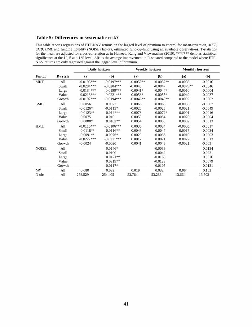
41

Table 5: Differences in systematic risk?

This table reports regressions of ETF-NAV returns on the lagged level of premium to control for mean-reversion, MKT,

SMB, HML and funding liquidity (NOISE) factors, estimated fund-by-fund using all available observations. T-statistics

for the mean are adjusted for cross-correlation as in Hameed, Kang and Viswanathan (2010). */**/*** denotes statistical

significance at the 10, 5 and 1 % level. ∆R2 is the average improvement in R-squared compared to the model where ETF-

NAV returns are only regressed against the lagged level of premium.

Daily horizon Weekly horizon Monthly horizon

Factor By style (a) (b) (a) (b) (a) (b)

MKT All -0.0193*** -0.0197*** -0.0050** -0.0052** -0.0036 -0.0016

Small -0.0204*** -0.0204*** -0.0048 -0.0047 -0.0079** -0.0046

Large -0.0184*** -0.0190*** -0.0041* -0.0044* -0.0016 -0.0004

Value -0.0216*** -0.0221*** -0.0053* -0.0055* -0.0049 -0.0037

Growth -0.0192*** -0.0194*** -0.0046** -0.0049** 0.0002 0.0002

SMB All 0.0056 0.0072 0.0066 0.0063 -0.0035 -0.0007

Small -0.0126* -0.0113* -0.0023 -0.0023 0.0021 -0.0049

Large 0.0123** 0.014*** 0.0078 0.0072* 0.0001 0.0016

Value 0.0075 0.010 0.0059 0.0054 0.0020 -0.0004

Growth 0.0088* 0.0102** 0.0054 0.0050 0.0002 0.0013

HML All -0.0116*** -0.0106*** 0.0030 0.0034 -0.0005 -0.0017

Small -0.0118** -0.0116** 0.0048 0.0047 -0.0017 -0.0034

Large -0.0091** -0.0076* 0.0029 0.0036 0.0010 0.0003

Value -0.0222*** -0.0211*** 0.0017 0.0021 0.0022 0.0013

Growth -0.0024 -0.0020 0.0041 0.0046 -0.0021 -0.003

NOISE All 0.0146* -0.0089 0.0134

Small 0.0100 0.0042 0.0221

Large 0.0171** -0.0165 0.0076

Value 0.0219** -0.0129 0.0079

Growth 0.0117* -0.0105 0.0131

∆R2 All 0.080 0.082 0.019 0.032 0.064 0.102

N obs All 258,529 254,405 53,764 53,288 13,664 13,502

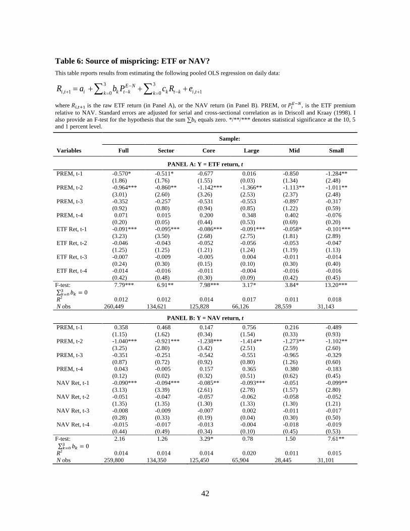
42

Table 6: Source of mispricing: ETF or NAV?

This table reports results from estimating the following pooled OLS regression on daily data:

3 3

, 1 , 10 0

E N

i t i k t k k t k i tk kR a b P c R e

where 𝑅𝑖,𝑡+1 is the raw ETF return (in Panel A), or the NAV return (in Panel B). PREM, or 𝑃𝑖𝐸−𝑁, is the ETF premium

relative to NAV. Standard errors are adjusted for serial and cross-sectional correlation as in Driscoll and Kraay (1998). I

also provide an F-test for the hypothesis that the sum ∑bk equals zero. */**/*** denotes statistical significance at the 10, 5 and 1 percent level.

Sample:

Variables Full Sector Core Large Mid Small

PANEL A: Y = ETF return, t

PREM, t-1 -0.570* -0.511* -0.677 0.016 -0.850 -1.284**

(1.86) (1.76) (1.55) (0.03) (1.34) (2.48)

PREM, t-2 -0.964*** -0.860** -1.142*** -1.366** -1.113** -1.011**

(3.01) (2.60) (3.26) (2.53) (2.37) (2.48)

PREM, t-3 -0.352 -0.257 -0.531 -0.553 -0.897 -0.317

(0.92) (0.80) (0.94) (0.85) (1.22) (0.59)

PREM, t-4 0.071 0.015 0.200 0.348 0.402 -0.076

(0.20) (0.05) (0.44) (0.53) (0.69) (0.20)

ETF Ret, t-1 -0.091*** -0.095*** -0.086*** -0.091*** -0.058* -0.101***

(3.23) (3.50) (2.68) (2.75) (1.81) (2.89)

ETF Ret, t-2 -0.046 -0.043 -0.052 -0.056 -0.053 -0.047

(1.25) (1.25) (1.21) (1.24) (1.19) (1.13)

ETF Ret, t-3 -0.007 -0.009 -0.005 0.004 -0.011 -0.014

(0.24) (0.30) (0.15) (0.10) (0.30) (0.40)

ETF Ret, t-4 -0.014 -0.016 -0.011 -0.004 -0.016 -0.016

(0.42) (0.48) (0.30) (0.09) (0.42) (0.45)

F-test:

∑ 𝑏𝑘 = 03𝑘=0

7.79*** 6.91** 7.98*** 3.17* 3.84* 13.20***

R2 0.012 0.012 0.014 0.017 0.011 0.018

N obs 260,449 134,621 125,828 66,126 28,559 31,143

PANEL B: Y = NAV return, t

PREM, t-1 0.358 0.468 0.147 0.756 0.216 -0.489

(1.15) (1.62) (0.34) (1.54) (0.33) (0.93)

PREM, t-2 -1.040*** -0.921*** -1.238*** -1.414** -1.273** -1.102**

(3.25) (2.80) (3.42) (2.51) (2.59) (2.60)

PREM, t-3 -0.351 -0.251 -0.542 -0.551 -0.965 -0.329

(0.87) (0.72) (0.92) (0.80) (1.26) (0.60)

PREM, t-4 0.043 -0.005 0.157 0.365 0.380 -0.183

(0.12) (0.02) (0.32) (0.51) (0.62) (0.45)

NAV Ret, t-1 -0.090*** -0.094*** -0.085** -0.093*** -0.051 -0.099**

(3.13) (3.39) (2.61) (2.78) (1.57) (2.80)

NAV Ret, t-2 -0.051 -0.047 -0.057 -0.062 -0.058 -0.052

(1.35) (1.35) (1.30) (1.33) (1.30) (1.21)

NAV Ret, t-3 -0.008 -0.009 -0.007 0.002 -0.011 -0.017

(0.28) (0.33) (0.19) (0.04) (0.30) (0.50)

NAV Ret, t-4 -0.015 -0.017 -0.013 -0.004 -0.018 -0.019

(0.44) (0.49) (0.34) (0.10) (0.45) (0.53)

F-test:

∑ 𝑏𝑘 = 03𝑘=0

2.16 1.26 3.29* 0.78 1.50 7.61**

R2 0.014 0.014 0.014 0.020 0.011 0.015

N obs 259,800 134,350 125,450 65,904 28,445 31,101

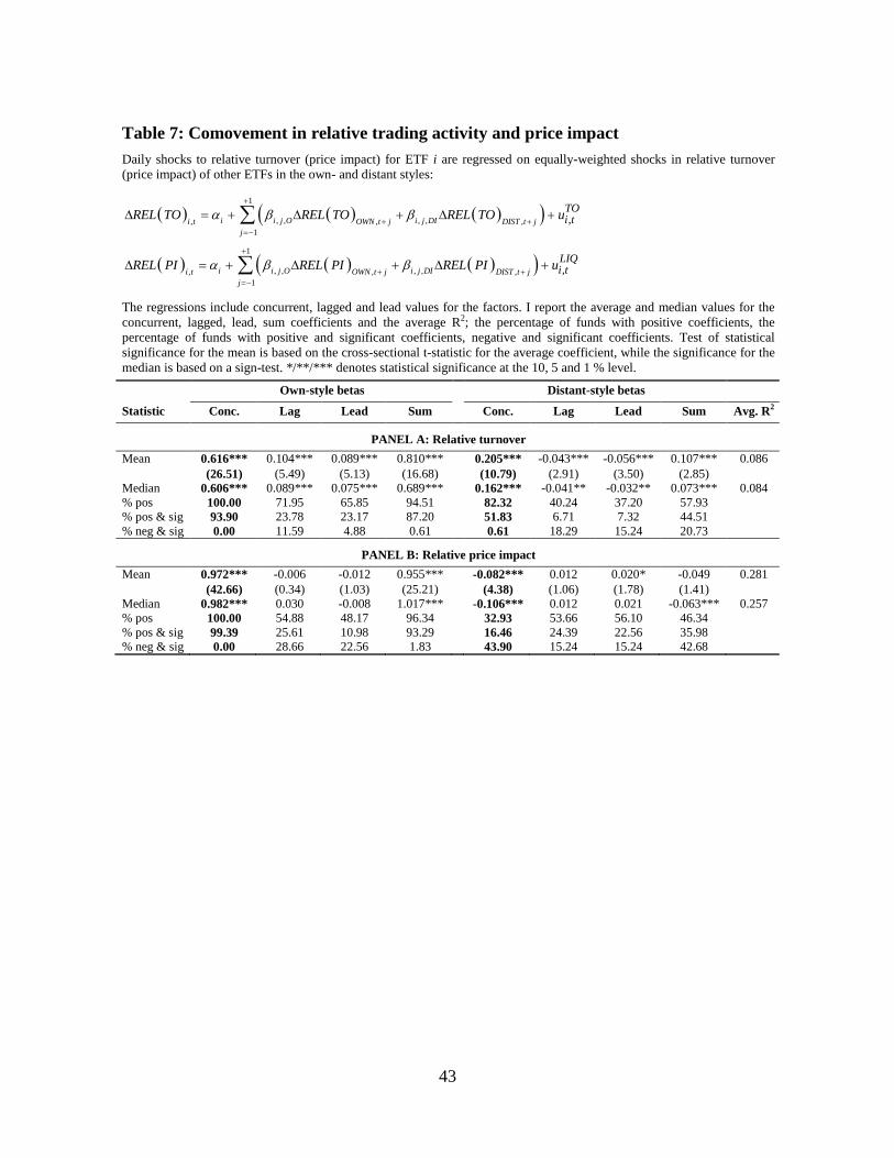
43

Table 7: Comovement in relative trading activity and price impact

Daily shocks to relative turnover (price impact) for ETF i are regressed on equally-weighted shocks in relative turnover

(price impact) of other ETFs in the own- and distant styles:

1

, , , ,, , ,

1

1

, , , ,, , ,

1

,

,

i i j O i j DIi t OWN t j DIST t j

j

i i j O i j DIi t OWN t j DIST t j

j

TOi t

LIQi t

REL TO REL TO REL TO u

REL PI REL PI REL PI u

The regressions include concurrent, lagged and lead values for the factors. I report the average and median values for the

concurrent, lagged, lead, sum coefficients and the average R2; the percentage of funds with positive coefficients, the

percentage of funds with positive and significant coefficients, negative and significant coefficients. Test of statistical

significance for the mean is based on the cross-sectional t-statistic for the average coefficient, while the significance for the

median is based on a sign-test. */**/*** denotes statistical significance at the 10, 5 and 1 % level.

Own-style betas Distant-style betas

Statistic Conc. Lag Lead Sum Conc. Lag Lead Sum Avg. R2

PANEL A: Relative turnover

Mean 0.616*** 0.104*** 0.089*** 0.810*** 0.205*** -0.043*** -0.056*** 0.107*** 0.086

(26.51) (5.49) (5.13) (16.68) (10.79) (2.91) (3.50) (2.85) Median 0.606*** 0.089*** 0.075*** 0.689*** 0.162*** -0.041** -0.032** 0.073*** 0.084

% pos 100.00 71.95 65.85 94.51 82.32 40.24 37.20 57.93

% pos & sig 93.90 23.78 23.17 87.20 51.83 6.71 7.32 44.51

% neg & sig 0.00 11.59 4.88 0.61 0.61 18.29 15.24 20.73

PANEL B: Relative price impact

Mean 0.972*** -0.006 -0.012 0.955*** -0.082*** 0.012 0.020* -0.049 0.281

(42.66) (0.34) (1.03) (25.21) (4.38) (1.06) (1.78) (1.41) Median 0.982*** 0.030 -0.008 1.017*** -0.106*** 0.012 0.021 -0.063*** 0.257

% pos 100.00 54.88 48.17 96.34 32.93 53.66 56.10 46.34

% pos & sig 99.39 25.61 10.98 93.29 16.46 24.39 22.56 35.98

% neg & sig 0.00 28.66 22.56 1.83 43.90 15.24 15.24 42.68

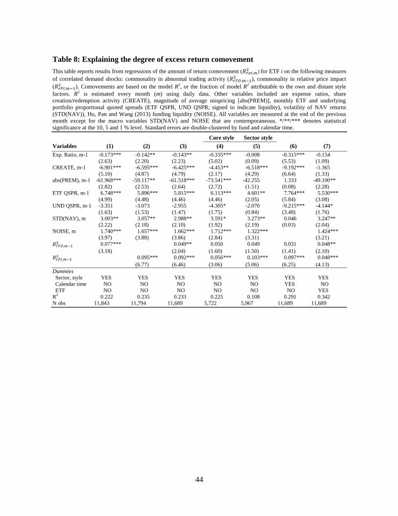
44

Table 8: Explaining the degree of excess return comovement

This table reports results from regressions of the amount of return comovement (𝑅𝑟𝑒𝑡,𝑚2 ) for ETF i on the following measures

of correlated demand shocks: commonality in abnormal trading activity (𝑅𝑟𝑇𝑂,𝑚−12 ), commonality in relative price impact

(𝑅𝑟𝑃𝐼,𝑚−12 ). Comovements are based on the model R2, or the fraction of model R2 attributable to the own and distant style

factors. R2 is estimated every month (m) using daily data. Other variables included are expense ratios, share

creation/redemption activity (CREATE), magnitude of average mispricing [abs(PREM)], monthly ETF and underlying

portfolio proportional quoted spreads (ETF QSPR, UND QSPR; signed to indicate liquidity), volatility of NAV returns

(STD(NAV)), Hu, Pan and Wang (2013) funding liquidity (NOISE). All variables are measured at the end of the previous

month except for the macro variables STD(NAV) and NOISE that are contemporaneous. */**/*** denotes statistical

significance at the 10, 5 and 1 % level. Standard errors are double-clustered by fund and calendar time.

Core style Sector style

Variables (1) (2) (3) (4) (5) (6) (7)

Exp. Ratio, m-1 -0.173*** -0.142** -0.143** -0.335*** -0.008 -0.315*** -0.154

(2.63) (2.20) (2.23) (5.02) (0.09) (5.53) (1.09)

CREATE, m-1 -6.901*** -6.595*** -6.425*** -4.453** -6.518*** -9.192*** -1.365

(5.10) (4.87) (4.79) (2.17) (4.29) (6.64) (1.33)

abs(PREM), m-1 -61.968*** -59.117** -61.518*** -73.541*** -42.255 1.333 -49.100**

(2.82) (2.53) (2.64) (2.72) (1.51) (0.08) (2.28)

ETF QSPR, m-1 6.748*** 5.896*** 5.815*** 6.113*** 4.601** 7.764*** 5.530***

(4.99) (4.48) (4.46) (4.46) (2.05) (5.84) (3.08)

UND QSPR, m-1 -3.351 -3.073 -2.955 -4.305* -2.070 -9.215*** -4.144*

(1.63) (1.53) (1.47) (1.75) (0.84) (3.48) (1.76)

STD(NAV), m 3.003** 3.057** 2.988** 3.591* 3.273** 0.046 3.247**

(2.22) (2.18) (2.10) (1.92) (2.19) (0.03) (2.04)

NOISE, m 1.740*** 1.657*** 1.662*** 1.712*** 1.322*** 1.424***

(3.97) (3.88) (3.86) (2.84) (3.31) (3.21)

𝑅𝑟𝑇𝑂,𝑚−12 0.077*** 0.049** 0.050 0.049 0.031 0.048**

(3.18) (2.04) (1.60) (1.50) (1.41) (2.10)

𝑅𝑟𝑃𝐼,𝑚−12 0.095*** 0.092*** 0.056*** 0.103*** 0.097*** 0.048***

(6.77) (6.46) (3.06) (5.06) (6.25) (4.13)

Dummies

Sector, style YES YES YES YES YES YES YES

Calendar time NO NO NO NO NO YES NO

ETF NO NO NO NO NO NO YES

R2 0.222 0.235 0.233 0.225 0.108 0.291 0.342

N obs 11,843 11,794 11,689 5,722 5,967 11,689 11,689