Bruno Avila Leal de Meirelles Herrera , Leandro dos Santos ... · PDF file466 QUANTUM INSPIRED PARTICLE SWARM COMBINED WITH LIN-KERNIGHAN-HELSGAUN METHOD ... (Parallelized Genetic

�

�

“main” — 2016/1/12 — 17:36 — page 465 — #1�

�

�

�

�

�

Pesquisa Operacional (2015) 35(3): 465-488© 2015 Brazilian Operations Research SocietyPrinted version ISSN 0101-7438 / Online version ISSN 1678-5142www.scielo.br/popedoi: 10.1590/0101-7438.2015.035.03.0465

QUANTUM INSPIRED PARTICLE SWARM COMBINEDWITH LIN-KERNIGHAN-HELSGAUN METHOD

TO THE TRAVELING SALESMAN PROBLEM

Bruno Avila Leal de Meirelles Herrera1, Leandro dos Santos Coelho2

and Maria Teresinha Arns Steiner3*

Received March 24, 2014 / Accepted May 2, 2015

ABSTRACT. The Traveling Salesman Problem (TSP) is one of the most well-known and studied problems

of Operations Research field, more specifically, in the Combinatorial Optimization field. As the TSP is a

NP (Non-Deterministic Polynomial time)-hard problem, there are several heuristic methods which have

been proposed for the past decades in the attempt to solve it the best possible way. The aim of this work

is to introduce and to evaluate the performance of some approaches for achieving optimal solution consid-

ering some symmetrical and asymmetrical TSP instances, which were taken from the Traveling Salesman

Problem Library (TSPLIB). The analyzed approaches were divided into three methods: (i) Lin-Kernighan-

Helsgaun (LKH) algorithm; (ii) LKH with initial tour based on uniform distribution; and (iii) an hybrid

proposal combining Particle Swarm Optimization (PSO) with quantum inspired behavior and LKH for lo-

cal search procedure. The tested algorithms presented promising results in terms of computational cost and

solution quality.

Keywords: Combinatorial Optimization, Traveling Salesman Problem, Lin-Kernighan-Helsgaun algo-

rithm, Particle Swarm Optimization with Quantum Inspiration.

1 INTRODUCTION

The Combinatorial Optimization problems are present in many situations of daily life. For this

reason, and because of the difficulty in solving them, these problems have increasingly drawn the

*Corresponding author.1Pos Graduacao em Engenharia de Producao de Sistemas (PPGEPS), Pontifıcia Universidade Catolica do Parana(PUCPR), Curitiba, PR, e Fundacao CERTI, Universidade Federal de Santa Catarina (UFSC), Florianopolis, SC, Brasil.E-mail: [email protected] Graduacao em Engenharia de Producao de Sistemas (PPGEPS), Pontifıcia Universidade Catolica do Parana(PUCPR), Curitiba, PR, e Pos Graduacao em Engenharia Eletrica (PPGEE), Universidade Federal do Parana (UFPR),Curitiba, PR, Brasil. E-mail: [email protected] Graduacao em Engenharia de Producao de Sistemas (PPGEPS), Pontifıcia Universidade Catolica do Parana(PUCPR), Curitiba, PR, e Pos Graduacao em Engenharia de Producao (PPGEP), Universidade Federal do Parana, Cu-ritiba, PR, Brasil. E-mail: [email protected]

�

�

“main” — 2016/1/12 — 17:36 — page 466 — #2�

�

�

�

�

�

466 QUANTUM INSPIRED PARTICLE SWARM COMBINED WITH LIN-KERNIGHAN-HELSGAUN METHOD

attention of many researches of various fields of knowledge who have made efforts to develop

ever efficient algorithms that can be appliedto such problems (Lawler et al., 1985).

Some of the examples of Combinatorial Optimization problems are: The Traveling SalesmanProblem (TSP), the Knapsack Problem, the Minimum Set Cover problem, the Minimum Span-ning Tree, the Steiner Tree problem and the Vehicle Routing problem (Lawler et al., 1985).

The TSP is defined as a set of cities and an objective function which involvesthe costs of travelling

from one city to the other. The aim of the TSP is to find a route (tour, path, itinerary) throughwhich the salesman would pass all the cities one single time, giving a minimum total distance.In other words, the aim of the TSP is to achieve a route that will form a Hamiltonian cycle

(or circuit) of minimum total cost (Pop et al., 2012).

The Combinatorial Optimization problems are used as models in many real situations (Robati etal., 2012; Lourenco et al., 2001; Johnson & McGeoch, 1997; Mosheiov, 1994; Sosa et al., 2007;Silva et al., 2009; Steiner et al., 2000), both in simple objective versions asin multiple criteria

versions (Ishibuchi & Murata, 1998; Jaszkiewicz, 2002). The Combinatorial optimization hasled many researchers to pursue approximate solutions of good quality and evenaccept that theyare considered insoluble in polynomial time.

On the other hand, many metaheuristic techniques have been developed and combined in order to

solve such problems: Dong et al. (2012) combine both Genetic Algorithm (GA) and Ant ColonyOptimization (ACO) together in a cooperative way to improve the performance of ACO forsolving TSPs. The mutual information exchange between ACO and GA in the end of the current

iteration ensures the selection of the best solutions for next iteration. In this way, this cooperativeapproach creates a better chance in reaching the global optimal solution because independentrunning of GA maintains a high level of diversity in next generation of solutions. Nagata & Soler

(2012) present a new competitive GA to solve the asymmetric TSP. The algorithm has beenchecked on a set of 153 benchmark instances with known optimal solution and it outperformsthe results obtained with previous ATSP (Asymmetric TSP) heuristic methods.

Sauer et al. (2008) used the following discrete Differential Evolution (DE) approaches for the

TSP: i) DE approach without local search, ii) DE with local search based on Lin-Kernighan-Heulsgaun (LKH) method, iii) DE with local search based on Variable Neighborhood Search(VNS) and together with LKH method. Numerical study was carried out using the TSPLIB of

TSP test problems. The obtained results show that LKH method is the best method to reachoptimal results for TSPLIB benchmarks but, for largest problems, the DE+VNS improve thequality of the obtained results.

Chen & Chien (2011a) make experiments using the 25 data sets from the TSPLIB (Travel-

ing Salesman Problem Library) and compare the experimental results of the proposed method(Genetic Simulated Annealing and Colony Systems with Particle Swarm Optimization, PSO)with many other methods. The experimental results show that both the mean solution and the

percentage deviation of the mean solution to the best known solution of the proposed methodare better than those methods. Chen & Chien (2011b) present in another paper another new

Pesquisa Operacional, Vol. 35(3), 2015

�

�

“main” — 2016/1/12 — 17:36 — page 467 — #3�

�

�

�

�

�

BRUNO MEIRELLES HERRERA, LEANDRO COELHO and MARIA TERESINHA STEINER 467

method (Parallelized Genetic Ant Colony System) for solving the TSP. It consists of the GA

with a new crossover operation and a hybrid mutation operation, and the ant colony systems withcommunication strategies. They also make an experiment with three classical data sets from theTSPLIB to test the performance of the proposed method, showing that it works very well.

Robati et al., 2012, present an extension of PSO algorithm which is in conformity with ac-tual nature is introduced for solving combinatorial optimization problems. Development of thisalgorithm is essentially based on balanced fuzzy sets theory. The balanced fuzzy PSO algorithm

is used for TSP.

Albayrak & Allhverdi (2011) developed a new mutation operator to increase GA performancein finding the shortest distance in the TSP. The method (Greedy Sub Tour Mutation) was testedwith simple GA mutation operator in 14 different TSP instances selected from TSPLIB. The new

method gives much more effective results regarding the best and mean error values. Liu & Zeng(2009) proposed an improved GA with reinforcement mutation to solve the TSP. The essence ofthis method lies in the use of heterogeneous pairing selection instead of random pairing selection

in EAX (edge assembly crossover) and in the construction of reinforcement mutation operator bymodifying the Q-learning algorithm and applying it to those individual generated from modifiedEAX. The experimental results on instances in TSPLIB have shown that this new method couldalmost get optimal tour every time, in reasonable time.

Puris et al. (2010) show how the quality of the solutions of ACO is improved by using a Two-Stage approach. The performance of this new approach is studied in the TSP and QuadraticAssignment Problem. The experimental results show that the obtained solutions are improvedin both problems using this approach. Misevieius et al. (2005) show the use of Iterated Tabu

search (ITS) technique combined with intensification and diversification for solving the TSP.This technique is combined to the 5-opt and, the errors are basically null in most of the TSPLIBtested problems. Wang et al. (2007) presented the use of PSO for solving the TSP with the use of

quantum principle in order to better guide the search for answers. The authors make comparisonswith Hill Climbing, Simulated Annealing and Tabu search, and show an example in which theresults of 14 cities are better this technique than with others.

However, on the other hand, during the last decade, the quantum computational theory had at-

tracted serious attention due to their remarkable superiority in computational and mechanicalaspects, which was demonstrated in Shor’s quantum factoring algorithm (Shor, 1994) andGrover’s database search algorithm (Grover, 1996). One of the recent developments in PSO is

the application of quantum laws of mechanics to observe the behavior of PSO. Such PSO’s arecalled quantum PSO (QPSO).

In QPSO, the particles are considered to lie in a potential field. The position of each particle isdepicted by using a wave function instead of position and velocity. Like PSO, QPSO is charac-

terized by its simplicity and easy implementation. Besides, it has better search ability and fewerparameters to set when compared against PSO (Fang et al., 2010). A convergence analysis ofQPSO is presented in Sun et al. (2012).


�

�

“main” — 2016/1/12 — 17:36 — page 468 — #4�

�

�

�

�

�


Comprehensively reviews of applications related to quantum algorithms and QPSO in the de-

sign and optimization of various problems in the engineering and computing fields have beenpresented in the recent literaturesuch as Fang et al. (2010) and Manju & Nigam (2014). Otherrecent and relevant optimization applications of the QPSO related to continuous optimization

can be mentioned too, such as feature selection and spiking neural network optimization(Hamedl et al., 2012), image processing (Li et al., 2015), economic load dispatch (Hossein-nezhad et al., 2014), multicast routing (Sun et al., 2011), heat exchangers design (Mariani et

al., 2012), inverse problems (Zhang et al., 2015), fuzzy system optimization (Lin et al., 2015),neuro-fuzzy design (Bagheri et al., 2014) and parameter estimation (Jau et al., 2013).

In terms of combinatorial optimization, this paper introduces a new hybrid optimization approachof Lin-Kernighan-Helsgaun technique (LKH) and quantum inspired particle swarm algorithm

for solving someTSP symmetric and asymmetric instances of the TSPLIB.

The rest of this paper is organized as follows: section 2 introduces a brief history of the TSP, aswell as some ways of solving it. Section 3 details the techniques approached in this paper: Lin-Kernighan (LK); Lin-Kernighan-Helsgaun (LKH); PSO and QPSO. In Section 4, the achieved

results are tabulated with the implement of the approached techniques for the instances of theTSLIB repository involving symmetric and asymmetric problems, and finally, section 5 presentsthe conclusions.

2 LITERATURE REVIEW

It is believed that one of the pioneer works about TSP was written by William Rowan Hamilton(Irish) and Thomas Penyngton Kirkman (British) in the XIX century based in a game in whichthe aim was to “travel” through 20 spots passing though only some specific connections allowedbetween the spots. Lawler et al. (1985) report that Hamilton was not the first one to introduce thisproblem, but his game helped him to promote it. The authors report yet that in modern days thefirst known mention to the TSP is attributed to Hassler Whitney, in 1934, in a work at PrincetonUniversity. Gradually, the amount of versions of the problem increased and some of them showpeculiarities that make their resolution easier. In the TSP, a trivial strategy for achieving optimalsolutions consists in evaluating all the feasible solutions and in choosing the one that minimizesthe sum of weights. The “only” inconvenience in this strategy is in the combinatorial explosion.For example, for a TSP with n cities connected in pairs, the number of feasible solutions is(n − 1)!/2.

The TSP can be represented as a permutation problem. Assuming Pn a collection of all per-mutations of the set A = {1, 2, . . . , n}, the aim for solving the TSP is to determine � =(�(1), �(2), . . . , �(n)) in Pn so that(

m−1∑i=1

d(c�(i), c�(i+1)

))+ d(c�(m), c�(1)

)will be minimized. For example, if n = 5 and � = (3, 4, 1, 5, 2) then the corresponding routewill be (3-4-1-5-2).


�

�

“main” — 2016/1/12 — 17:36 — page 469 — #5�

�

�

�

�

�


Mathematically the TSP is defined as a decision problem and not an optimization problem. Thus,the fundamental answer that must be given is whether there is or not a route with a minimumtotal distance. In such context, the decision problem can be modeled as follows. Given a finiteset C = {c1, c2, . . . , cm} of cities in d(ci , c j ) ∈ Z+ distance for each pair of cities ci , c j ∈ C,and the total initial cost T ∈ Z+, where Z+ is the set of positive integers such as inequation (1)is met. (

m−1∑i=1

d(c�(i), c�(i+1)

))+ d(c�(m), c�(1)

) ≤ T (1)

According to Lawler et al. (1985), many techniques have been developed over the years in orderto construct exact algorithms that would solve the TSP, such as Dynamic Programming, Brach-and-Bound and Cutting-plane methods (Papadimitriou & Steiglitz, 1982; Nemhauser & Wolsey,1988; Hoffmann, 2000). However, the computational trimmings to solving large instances ofexact algorithms are unfeasible/prohibitive.

Therefore, we use heuristic methods that are able, in a general way, to provide satisfactory re-sponses to the TSPs. Initially, the researchers used techniques considered greedy or myopic forthe development of such algorithms (Lawler et al., 1985), such as the Nearest neighbor method,the insertion method, methods for route improvement, such as k-opt (Laport, 1992) and Lin-Kernighan (LK) (Lin & Kernighan, 1973). It is necessary to emphasize that the LK method is arelatively old method, but it is still widely disseminated among the studies related to achievingpromising solutions for the TSP since it is one of the most powerful and robust methods for thatapplication.

A disadvantage of the heuristics lays in the difficulty of “escaping” from optimum places. Thisfact gave origin to another class of methodologies known as metaheuristics which have tools thatallow the “escaping” from these optimum placesin a way that the search can be done in morepromising regions. The challenge is to produce, in minimal time, solutions that are as close aspossible to the optimum solution.

It must be noted that in terms of metaheuristics, a promising approach is the Particle SwarmOptimization (PSO). The PSO algorithm was developed initially by Kennedy and Eberhart(Kennedy & Eberhart, 1995) based on the studies of the socio-biologist Edward Osborne Wilson(Wilson, 1971). The base of the development of the PSO algorithm is a hypothesis in which theexchange of information between beings of the same specie offers an evolutionary advantage.

Another recent approach is the use of concepts of Quantum mechanics (QM) (Pang, 2005) andalso of Quantum Computation (QC) (Chung & Nielsen, 2000) in the design of optimizationalgorithms (Hogg & Portnov, 2000; Protopescu & Barhen, 2002; Coelho, 2008). The QM is amathematical structure, or a set of rules, for the construction of physics theories. The QC wasintroduced by Benioff (1980) and Feynman (1982), and it is a research field in rapid growth inrecent years. The concepts from QM (superposition of states; inference; delta potential energyand Schrodinger’s equation) and of the QC (quantum bits, or qu-bits; quantum gates and parallelprocessing) have been explored for the creation of new methods or even for the enhancement ofthe efficiency of the existing optimization methods.


�

�

“main” — 2016/1/12 — 17:36 — page 470 — #6�

�

�

�

�

�


The quantum world is inexplicable in terms of the classical mechanics. The previsions from the

interactions of matter and light in Newton’s law for particle movement, and the equations ofMaxwell that control the propagation of electromagnetic fields are contradictory in experimentsperformed in microscopic scale. Obviously, there must be a limit line of the size of the objects

so that their behavior fit in classical mechanics or in QM. In this limit line, there are objectsthat are approximately 100 times bigger than a hydrogen atom. The objects that are smaller thanthat have their behaviors described in QM, and the objects that are bigger are described by the

Newtonian mechanics.

The QM is a remarkable theory. There seems to be no real doubt that much of that in physicsand all in chemistry would be deductible from its postulates or laws. QM has answered manyquestions correctly and given a deeper view of natural processes, and it is willing to contribute

even more. It is a wide theory on which is based much of our knowledge about mechanics andradiation. It is a relatively recent theory. In 1900, the matter mechanics, based on Newton’s lawof motion, had resisted changesfor centuries. In the same way, the ondulatory theory of light,

based in the electromagnetic theory, resisted with no challenges (Pohl, 1971).

It is true that QM has not yet presented a consistent description of elementary particles and ofiteration fields; however the theory is already completed to be used in experiments with atoms,molecules, nuclei, radiations and solids. As a result of the expansive growth of this theory in the

half of XX century, we can see its great progress in this century (Merzbacher, 1961).

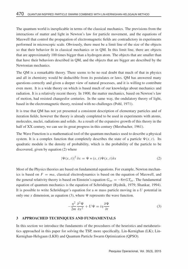
The Wave Function is a mathematical tool of the quantum mechanics used to describe a physicalsystem. It is a complex function that completely describes the state of a particle �(x, t). Itsquadratic module is the density of probability, which is the probability of the particle to be

discovered, given by equation (2) where

|�(x, t)|2 ∂x = � ∗ (x, t)�(x, t)∂x (2)

Most of the Physics theories are based on fundamental equations. For example, Newton mechan-ics is based on F = ma, classical electrodynamics is based on the equation of Maxwell, and

the general relativity theory is based on Einstein’s equation Guv = −8πGTuv . The fundamentalequation of quantum mechanics is the equation of Schrodinger (Rydnik, 1979; Shankar, 1994).It is possible to write Schrodinger’s equation for a m mass particle moving in a U potential in

only one x dimension, as equation (3), where � represents the wave function.

− η2

2m

∂2�

∂x2+U� = iη

∂�

∂t(3)

3 APPROACHED TECHNIQUES AND FUNDAMENTALS

In this section we introduce the fundaments of the procedures of the heuristics and metaheuris-

tics approached in this paper for solving the TSP, more specifically, Lin-Kernighan (LK); Lin-Kernighan-Helsgaun (LKH) and Quantum Particle Swarm Optimization (QPSO).


�

�

“main” — 2016/1/12 — 17:36 — page 471 — #7�

�

�

�

�

�


3.1 Lin-Kernighan Heuristic (LK)

An important set of heuristics developed for the TSP is made of the k-opt exchanges. In general,these are algorithms that starting from an initial feasible solution for the TSP transposes λ arcs

that are in the circuit for another λ arcs outside it, keeping in mind the reduction of the total costof the circuit at each exchange.

The first exchange mechanism known as 2-opt was introduced by Croes (1958). In this mech-anism a solution is generated through the removal of two arcs, resulting in two paths. One of

the paths is inverted and then reconnected in order to form a new route. This new solution thenbecomes the current solution and the process is repeated until it is not possible to perform a newexchange of two arcs, with gain. Shen Lin (1965) proposes a wider neighborhood when con-

sidering all the possible solutions with the exchange of three arcs, the 3-opt. Lin & Kernighan(1973) propose an algorithm in which the number of arcs exchanged in each step is variable. Thearc exchanges (k-opt) are performed according to a criterion of gain that restricts the size of the

searched neighborhood.

The LK heuristic is considered to be one of the most efficient methods in generating optimal ornear-optimum solutions for the symmetric TSP. However, the design and the implementation ofan algorithm based on this heuristic are not trivial. There are many decisions that must be made

and most of them greatly influence in its performance. The number of operations to test all theexchanged λ increases rapidly as the number of cities increases.

In a simple implementation, the algorithm used to test the k-exchanges has the complexity ofO(nλ). As a consequence, the values k = 2 and k = 3 are the ones used the most. In Christo-

fides & Elion (1972), we see k = 4 and k = 5 been used. An inconvenience of this algorithmis that λ must be detailed in the beginning of the execution. And it is hard to know which valuemust be used for λ in order to obtain the best cost-benefit between the time of implement and the

quality of solution.

Lin & Kernighan (1973) removed this inconvenience of the k − opt algorithm by introducingthe k-opt variable. This algorithm can vary the value of λ during the implement, deciding at eachiteration which value λ must assume. At each iteration, the algorithm searches through increasing

values of λ which variation makes up the shortest route. Given a number of exchanges r, a seriesof tests are performed in order to verify when r + 1 exchange must be considered. This happensup to the point that some stop condition is met.

At each step the algorithm considers an increasing number of possible exchanges, starting in

r = 2. These exchanges are chosen in a way that the viability of the route can be achieved inany stage of the process. If the search for a shorter route is successful then the previous route isdiscarded and replaced by the new route.

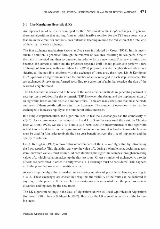
The LK algorithm belongs to the class of algorithms known as Local Optimization Algorithms

(Johnson, 1990; Johnson & Mcgeoh, 1997). Basically, the LK algorithm consists of the follow-ing steps:


�

�

“main” — 2016/1/12 — 17:36 — page 472 — #8�

�

�

�

�

�


(i) Generate a random starting tour T .

(ii) Set G∗ = 0. (G∗ represents the best improvement made so far). Choose any node t1 and letx1 be one of the adjacent arcs of T to t1. Let i = 1.

(iii) From the other endpoint t2 of x1, choose y1 to t3 with g1 = |x1| − |y1| > 0. If no such y1

exists, go to (vi)(d).

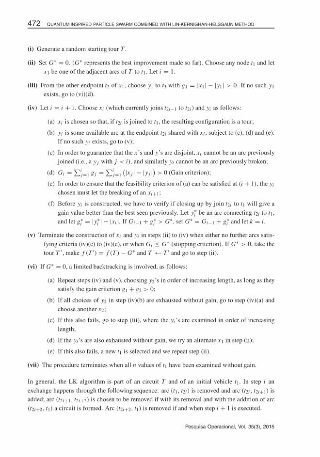
(iv) Let i = i + 1. Choose xi (which currently joins t2i−1 to t2i ) and yi as follows:

(a) xi is chosen so that, if t2i is joined to t1, the resulting configuration is a tour;

(b) yi is some available arc at the endpoint t2i shared with xi , subject to (c), (d) and (e).If no such yi exists, go to (v);

(c) In order to guarantee that the x’s and y’s are disjoint, xi cannot be an arc previouslyjoined (i.e., a y j with j < i), and similarly yi cannot be an arc previously broken;

(d) Gi =∑ij=1 g j =∑i

j=1

(|x j | − |y j |)

> 0 (Gain criterion);

(e) In order to ensure that the feasibility criterion of (a) can be satisfied at (i + 1), the yi

chosen must let the breaking of an xi+1;

(f) Before yi is constructed, we have to verify if closing up by join t2i to t1 will give a

gain value better than the best seen previously. Let y∗i be an arc connecting t2i to t1,and let g∗i = |y∗i | − |xi |. If Gi−1 + g∗i > G∗, set G∗ = Gi−1 + g∗i and let k = i.

(v) Terminate the construction of xi and yi in steps (ii) to (iv) when either no further arcs satis-

fying criteria (iv)(c) to (iv)(e), or when Gi ≤ G∗ (stopping criterion). If G∗ > 0, take thetour T ’, make f (T ′) = f (T )− G∗ and T ← T ′ and go to step (ii).

(vi) If G∗ = 0, a limited backtracking is involved, as follows:

(a) Repeat steps (iv) and (v), choosing y2’s in order of increasing length, as long as theysatisfy the gain criterion g1 + g2 > 0;

(b) If all choices of y2 in step (iv)(b) are exhausted without gain, go to step (iv)(a) and

choose another x2;

(c) If this also fails, go to step (iii), where the yi ’s are examined in order of increasing

length;

(d) If the yi ’s are also exhausted without gain, we try an alternate x1 in step (ii);

(e) If this also fails, a new t1 is selected and we repeat step (ii).

(vii) The procedure terminates when all n values of t1 have been examined without gain.

In general, the LK algorithm is part of an circuit T and of an initial vehicle t1. In step i an

exchange happens through the following sequence: arc (t1, t2i) is removed and arc (t2i , t2i+1) isadded; arc (t2i+1, t2i+2) is chosen to be removed if with its removal and with the addition of arc(t2i+2, t1) a circuit is formed. Arc (t2i+2, t1) is removed if and when step i + 1 is executed.


�

�

“main” — 2016/1/12 — 17:36 — page 473 — #9�

�

�

�

�

�


The number of insertions and removals in the search process is limited by the gain criterion ofLK. Basically, this criterion limits the sequence of the exchanges to those that result in posi-tive gains (route size reduction) at each step of the sequence; at first, sequences in which theexchanges result in positive gain and others in negative gains are not taken into account, butinstead, those in which the total gain is positive.

Another mechanism in this algorithm is the analysis of alternative solutions every time a newsolution with zero gain is generated (step (vi)). This is done by choosing new arcs for theexchange.

3.2 Lin-Kernighan Heuristic (LKH)

Keld Helsgaun (2000) revises the original Lin-Kernighan algorithm and proposes and devel-ops modifications that improve its performance. Efficiency is increased, firstly, by revising theheuristic rules of Lin & Kernighan in order to restrict and direct the search. Despite the naturalappearance of these rules, a critical analysis will show that they have considerable deficiencies.

By analyzing the rules of the LK algorithm that are used for refining the search, Helsgaun(2000) not only saved computational time but also identified a problem that could lead the algo-rithm to find poor solutions for greater problems. One of the rules proposed by Lin & Kernighan(Lin & Kernighan, 1973) limits the search refining it to embrace only the closest five neigh-bors. In this case, if a neighbor that would provide the optimum result is not one of these fiveneighbors the search will not lead to an optimal result. Helsgaun (2000) uses as an example theatt532 problem of the TSPLIB, by Padberg & Rinaldi (1987) in which the best neighbor is onlyfound on the 22nd search.

Considering that fact, Helsgaun (2000) introduces a proximity measure that better reflects thepossibility of getting an edge that is part of the optimum course. This measure is called α-nearness, it is based on the sensibility analysis using a minimum spanning tree 1-trees. At leasttwo small changes are performed in the basic motion in the general scheme. First, in a specialcase, the first motion of a sequence must be a 4-opt sequential motion; the following motion mustbe the 2-opt motion. In second place, the non-sequential 4-opt motion are tested when the coursecannot be improved by sequential motion.

Moreover, the modified LKH algorithm revises the basic structure of the search in other points.The first and most important point is the change of the basic 4-opt motion to a sequential 5-opt motion. Besides this one, computational experiences show that the backtracking is not sonecessary in this algorithm and its removal reduces the execution time; it does not compromisesthe final performance of the algorithm and it extremely simplifies the execution.

Regarding the initial course, the LK algorithm performs edge exchanges many times in the sameproblem using different initial courses. The experiences with many execution of the LKH algo-rithm show that the quality of the final solutions does not depend that much on the initial solu-tions. However, the significant reduction in time can be achieved, as for example, by choosinginitial solutions that are closer to optimum through constructive heuristics. Thus, Helsgaun alsointroduces in his work a simple heuristic that was used in the construction of initial solutions inhis version of the LK (Lawler et al., 1985).


�

�

“main” — 2016/1/12 — 17:36 — page 474 — #10�

�

�

�

�

�


On the other hand, Nguyen et al. (2006) affirms that the use of the 5-opt movement as a basicmotion greatly increases the necessary computational time, although the solutions that are foundare of really good quality. Besides that, the consumption of memory and necessary time for thepre-processing of the LKH algorithm are very high when compared to other implementationsof LK.

3.3 QPSO (Quantum Particle Swarm Optimization)

The Particle Swarm Optimization (PSO) algorithm introduced in 1995 by James Kennedy &Russel Eberhart is based on bird’s collective behaviors (Kennedy & Eberhart, 1995). The PSOalgorithm is a technique of collective intelligence based in a population of solutions and ran-dom transitions. The PSO algorithm has similar characteristics to the ones of the evolutionarycomputation which are based on a population of solutions. However, the PSO is motivated bythe simulation of social behavior and cooperation between agents instead of the survival of theindividual that is more adaptable as it is in the evolutionary algorithms. In the PSO algorithm,each candidate solution (named particle) is associated to a velocity vector. The velocity vectoris adjusted through an updating equation which considers the experience of the correspondingparticle and the experience of the other particles in the population.

The PSO algorithm concept consists in changing the velocity of each particle in direction to thepbest (personal best) and gbest (global best) localization at each interactive step. The velocityof the search procedure is weighted by a term that is randomly generated, and that is separatelylinked to the localizations of the pbest and of the gbest. The procedure for implementation of thealgorithm PSO is regulated by the following steps (Herrera & Coelho, 2006; Coelho & Herrera,2006; Coelho, 2008):

(i) Initiate randomly and with uniform distribution a particle population (matrix) with posi-tions and speed in an space of n dimensional problem;

(ii) For each particle evaluate the aptitude function (objective function to be minimized, inthis case, the TSP optimization);

(iii) Compare the evaluation of the aptitude function of the particle with the pbest of the par-ticle. If the current value is better than pbest, then the pbest value becomes equal to thevalue of the particle aptitude, and the localization of the pbest becomes equal to the currentlocalization in n dimensional space;

(iv) Compare the evaluation of the aptitude function with the population best previous aptitudevalue. If the current value is better than the gbest, update the gbest value for the index andthe current particle value;

(v) Modify speed and position of the particle according to the equations (4) and (5), respec-tively, where t is equal to 1.

vi (t + 1) = w · vi (t)+ c1 · ud · [pi (t)− xi(t)]+ c2 ·Ud · [pg(t)− xi(t)

](4)

xi(t + 1) = xi(t)+t · vi (t + 1) (5)


�

�

“main” — 2016/1/12 — 17:36 — page 475 — #11�

�

�

�

�

�


(vi) Go to step (ii) until a stop criterion is met (usually a value of error pre-defined or a maxi-mum number of iterations).

We use the following notations: t is the iteration (generation), xi = [xi1, xi2, . . . , xin]T stores theposition of the i-th particle, vi = [vi1, vi2, . . . , vin ]T stores the velocity of the i-th particle andpi = [pi1, pi2, . . . , pin ]T represents the position of the best fitness value of the i-th particle. Theindex g represents the index of the best particle among all particles of the group. The variable

w is the weight of inertia; c1 and c2 are positive constants; ud and Ud are two functions for thegeneration of random numbers with uniform distribution in the intervals [0, 1], respectively. Thesize of the population is selected according to the problem.

The particle velocities in each dimension are limited to a maximum value of velocity, Vmax.The Vmax is important because it determines the resolution in which the regions that are nearthe current solutions are searched. If Vmax is high, the PSO algorithm makes the global searcheasy, while a small Vmax value emphasizes the local search. The firs term of equation (4) repre-

sents the term of the particle moment, where the weight of the inertia w represents the degreeof the moment of the particle. The second term consist in the “cognitive” part, which repre-sents the independent “knowledge” of the particle, and the third term consist in the “social” that

represents cooperation among particles.

The constants c1 and c2 represent the weight of the “cognition” and “social” parts, respectively,and they influence each particle directing them to the pbest and the gbest. These parameters areusually adjusted by trial-and-error heuristics.

The Quantum PSO (QPSO) algorithm allows the particles to move following the rules defined

by the quantum mechanics instead of the classical Newtonian random movement (Sun et al.,2004a, 2004b). In the quantum model of the PSO, the state of each particle is represented bya wave function �(x , t) instead of the velocity position as it is in the conventional model. The

dynamic behavior of the particle is widely divergent of the PSO traditional behavior, where exactvalues and velocities and positions cannot be determined simultaneously. It is possible to learnthe probability of a particle to be in a certain position through the probability of its density

function |�(x , t)|2 which depends on the potential field in which the particle is.

In Sun et al. (2004a) and Sung et al. (2004b), the wave function of the particle can be defined byequation (6) where

�(x) = 1√L· e−‖p−x‖

L (6)

and the density of probability is given by the following expression (7).

Q(x) = |�(x)|2 = 1

L· e−2‖p−x‖

L (7)

The L parameter depends on the intensity of energy in the potential field, which defines the scope

of search of the particle and can be called the Creativity or Imagination of the particle (Sun etal., 2004b).


�

�

“main” — 2016/1/12 — 17:36 — page 476 — #12�

�

�

�

�

�


In the quantum inspired PSO model, the search space and the solution space is different in

quality. The wave function or the probability function describes the state of the particle in aquantum search space, and it does not provide any information of the position of the particle,what is mandatory to calculate the cost function.

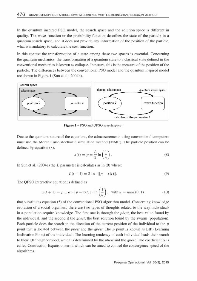
In this context the transformation of a state among these two spaces is essential. Concerning

the quantum mechanics, the transformation of a quantum state to a classical state defined in theconventional mechanics is known as collapse. In nature, this is the measure of the position of theparticle. The differences between the conventional PSO model and the quantum inspired model

are shown in Figure 1 (Sun et al., 2004b).

Figure 1 – PSO and QPSO search space.

Due to the quantum nature of the equations, the admeasurements using conventional computersmust use the Monte Carlo stochastic simulation method (MMC). The particle position can be

defined by equation (8).

x(t) = p ± L

2ln

(1

n

). (8)

In Sun et al. (2004a) the L parameter is calculates as in (9) where:

L(t + 1) = 2 · α · ‖p − x(t)‖. (9)

The QPSO interactive equation is defined as

x(t + 1) = p ± α · ‖p− x(t)‖ · ln(

1

u

), with u = rand (0, 1) (10)

that substitutes equation (5) of the conventional PSO algorithm model. Concerning knowledge

evolution of a social organism, there are two types of thoughts related to the way individualsin a population acquire knowledge. The first one is through the pbest, the best value found bythe individual, and the second it the gbest, the best solution found by the swarm (population).

Each particle does the search in the direction of the current position of the individual to the ppoint that is located between the pbest and the gbest. The p point is known as LIP (LearningInclination Point) of the individual. The learning tendency of each individual leads their search

to their LIP neighborhood, which is determined by the pbest and the gbest. The coefficient α iscalled Contraction-Expansion term, which can be tuned to control the convergence speed of thealgorithms.


�

�

“main” — 2016/1/12 — 17:36 — page 477 — #13�

�

�

�

�

�


In the QPSO algorithm, each particle records its pbest and compares it to all the other particles

of the population in order to get the gbest at each iteration. In order to execute the next step,the L parameter is calculated. The L parameter is considered to be the Creativity or Imaginationof the particle, and therefore it is characterized as the scope of search of the knowledge of the

particle. The greater the value of L , the easier the particle acquires new knowledge. In the QPSOthe Creativity factor of the particle is calculates as the difference between the current position ofthe particle and its LIP, as shown in equation (9).

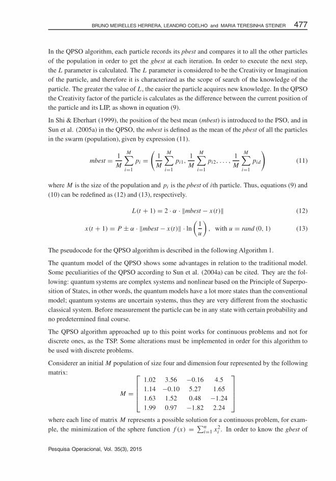
In Shi & Eberhart (1999), the position of the best mean (mbest) is introduced to the PSO, and in

Sun et al. (2005a) in the QPSO, the mbest is defined as the mean of the pbest of all the particlesin the swarm (population), given by expression (11).

mbest = 1

M

M∑i=1

pi =(

1

M

M∑i=1

pi1,1

M

M∑i=1

pi2, . . . ,1

M

M∑i=1

pid

)(11)

where M is the size of the population and pi is the pbest of ith particle. Thus, equations (9) and

(10) can be redefined as (12) and (13), respectively.

L(t + 1) = 2 · α · ‖mbest − x(t)‖ (12)

x(t + 1) = P ± α · ‖mbest − x(t)‖ · ln(

1

u

), with u = rand (0, 1) (13)

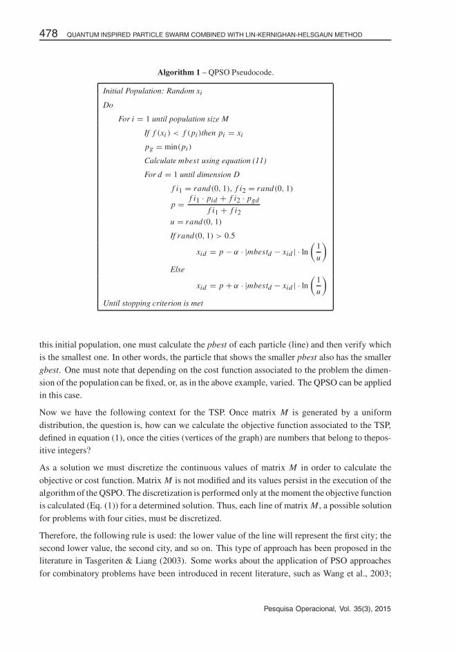
The pseudocode for the QPSO algorithm is described in the following Algorithm 1.

The quantum model of the QPSO shows some advantages in relation to the traditional model.Some peculiarities of the QPSO according to Sun et al. (2004a) can be cited. They are the fol-

lowing: quantum systems are complex systems and nonlinear based on the Principle of Superpo-sition of States, in other words, the quantum models have a lot more states than the conventionalmodel; quantum systems are uncertain systems, thus they are very different from the stochastic

classical system. Before measurement the particle can be in any state with certain probability andno predetermined final course.

The QPSO algorithm approached up to this point works for continuous problems and not fordiscrete ones, as the TSP. Some alterations must be implemented in order for this algorithm to

be used with discrete problems.

Considerer an initial M population of size four and dimension four represented by the followingmatrix:

M =

⎡⎢⎢⎢⎣

1.02 3.56 −0.16 4.51.14 −0.10 5.27 1.651.63 1.52 0.48 −1.24

1.99 0.97 −1.82 2.24

⎤⎥⎥⎥⎦

where each line of matrix M represents a possible solution for a continuous problem, for exam-

ple, the minimization of the sphere function f (x) = ∑ni=1 x2

i . In order to know the gbest of


�

�

“main” — 2016/1/12 — 17:36 — page 478 — #14�

�

�

�

�

�


Algorithm 1 – QPSO Pseudocode.

Initial Population: Random xi

Do

For i = 1 until population size M

If f (xi ) < f (pi )then pi = xi

pg = min(pi )

Calculate mbest using equation (11)

For d = 1 until dimension D

f i1 = rand(0, 1), f i2 = rand(0, 1)

p = f i1 · pid + f i2 · pgd

f i1 + f i2u = rand(0, 1)

If rand(0, 1) > 0.5

xid = p − α · |mbestd − xid | · ln(

1

u

)Else

xid = p + α · |mbestd − xid | · ln(

1

u

)Until stopping criterion is met

this initial population, one must calculate the pbest of each particle (line) and then verify whichis the smallest one. In other words, the particle that shows the smaller pbest also has the smaller

gbest. One must note that depending on the cost function associated to the problem the dimen-sion of the population can be fixed, or, as in the above example, varied. The QPSO can be appliedin this case.

Now we have the following context for the TSP. Once matrix M is generated by a uniform

distribution, the question is, how can we calculate the objective function associated to the TSP,defined in equation (1), once the cities (vertices of the graph) are numbers that belong to thepos-itive integers?

As a solution we must discretize the continuous values of matrix M in order to calculate the

objective or cost function. Matrix M is not modified and its values persist in the execution of thealgorithm of the QSPO. The discretization is performed only at the moment the objective functionis calculated (Eq. (1)) for a determined solution. Thus, each line of matrix M , a possible solution

for problems with four cities, must be discretized.

Therefore, the following rule is used: the lower value of the line will represent the first city; thesecond lower value, the second city, and so on. This type of approach has been proposed in theliterature in Tasgeriten & Liang (2003). Some works about the application of PSO approaches

for combinatory problems have been introduced in recent literature, such as Wang et al., 2003;


�

�

“main” — 2016/1/12 — 17:36 — page 479 — #15�

�

�

�

�

�


Pang et al., 2004a; Pang et al., 2004b; Machado & Lopes, 2005; Lopes & Coelho, 2005, but none

of them using QPSO.

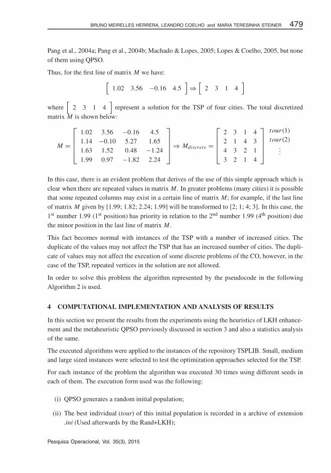
Thus, for the first line of matrix M we have:[1.02 3.56 −0.16 4.5

]⇒[

2 3 1 4]

where[

2 3 1 4]

represent a solution for the TSP of four cities. The total discretized

matrix M is shown below:

M =

⎡⎢⎢⎢⎣

1.02 3.56 −0.16 4.51.14 −0.10 5.27 1.651.63 1.52 0.48 −1.24

1.99 0.97 −1.82 2.24

⎤⎥⎥⎥⎦⇒ Mdiscrete =

⎡⎢⎢⎢⎣

2 3 1 42 1 4 34 3 2 1

3 2 1 4

⎤⎥⎥⎥⎦

tour(1)

tour(2)...

In this case, there is an evident problem that derives of the use of this simple approach which is

clear when there are repeated values in matrix M . In greater problems (many cities) it is possiblethat some repeated columns may exist in a certain line of matrix M; for example, if the last lineof matrix M given by [1.99; 1.82; 2.24; 1.99] will be transformed to [2; 1; 4; 3]. In this case, the

1st number 1.99 (1st position) has priority in relation to the 2nd number 1.99 (4th position) duethe minor position in the last line of matrix M .

This fact becomes normal with instances of the TSP with a number of increased cities. Theduplicate of the values may not affect the TSP that has an increased number of cities. The dupli-

cate of values may not affect the execution of some discrete problems of the CO, however, in thecase of the TSP, repeated vertices in the solution are not allowed.

In order to solve this problem the algorithm represented by the pseudocode in the followingAlgorithm 2 is used.

4 COMPUTATIONAL IMPLEMENTATION AND ANALYSIS OF RESULTS

In this section we present the results from the experiments using the heuristics of LKH enhance-ment and the metaheuristic QPSO previously discussed in section 3 and also a statistics analysisof the same.

The executed algorithms were applied to the instances of the repository TSPLIB. Small, mediumand large sized instances were selected to test the optimization approaches selected for the TSP.

For each instance of the problem the algorithm was executed 30 times using different seeds ineach of them. The execution form used was the following:

(i) QPSO generates a random initial population;

(ii) The best individual (tour) of this initial population is recorded in a archive of extension.ini (Used afterwards by the Rand+LKH);


�

�

“main” — 2016/1/12 — 17:36 — page 480 — #16�

�

�

�

�

�


(iii) QPSO is executed until it finds the best global for the population randomly generated;

(iv) The best global (tour) is recorded in an archive with extension .final;

(v) The LKH is executed using as the initial tour the archive (*.ini) (Rand+LK approach);

(vi) The LKH is executed using as the initial tour the archive (.final) (QPSO+LK Approach);

(vii) The LKH is executed with default parameters (pure LKH).

The size of the populations was fixed in 100 particles and the stop criterion was the optimumvalue mentioned in the TSPLIB for the approached problem. In the case of the QPSO withoutLKH, the stopping criterion was a fixed iterations number previously defined as 1000.

In QPSO, Contraction-Expansion Coefficient α is a vital parameter to the convergence of theindividual particle in QPSO, and therefore exerts significant influence on convergence of thealgorithm. Mathematically, there are many forms of convergence of stochastic process, and dif-ferent forms of convergence have different conditions that the parameter must satisfy. An effi-cient method is linear-decreasing method that decreasing the value of α linearly as the algorithmis running. In this paper, α is adopted with value 1.0 at the beginning of the search to 0.5 at theend of the search for all optimization problems (Sun et al., 2005b).

4.1 Results for the Symmetric TSP

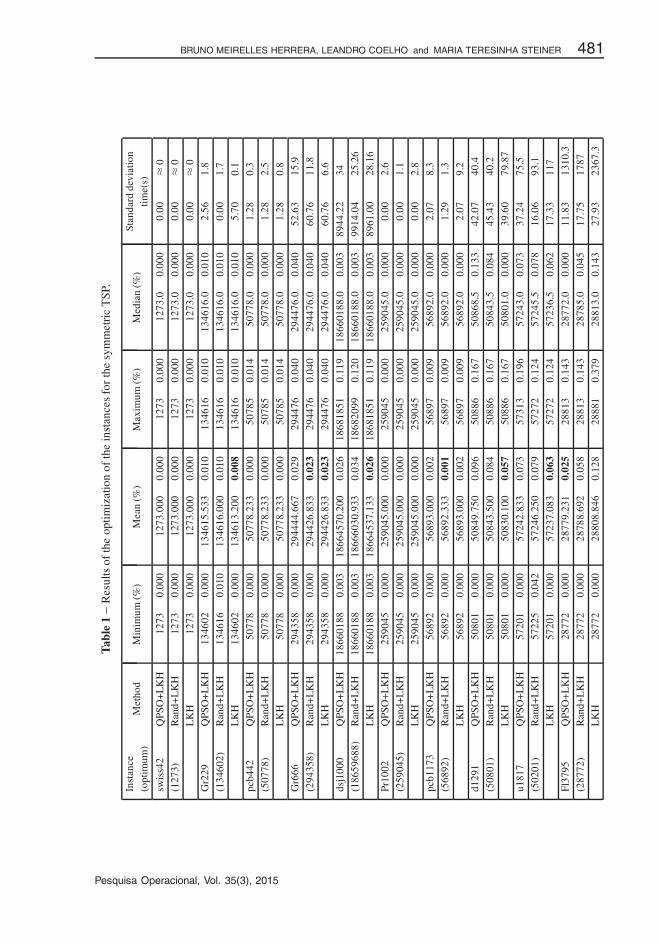
Table 1 shows the results for the algorithms: (i) QPSO+LKH, (ii) Rand +LKH, and (iii) LKH,for 10 test problems from the TSPLIB (Reinelt, 1994). The notation “%” was used in this table torepresent how much a value for the test problem is distant from the optimum value in percentage.

Note by the results in Table 1 that for the problem swiss42 (Reinelt, 1994), the algorithmsQPSO+LKH, Rand+LKH and LKH showed similar performance, including in the statisticalanalysis by obtaining the best value (optimum value) for the objective function of 1273. Re-garding the problem Gr229, the algorithm Rand+LKH did not achieved the optimum value of134602, instead, 0.010% of this value. However, the QPSO+LKH and the LKH achieved opti-mum value. The LKH was in mean slightly superior to the QPSO+LKH.

For the problem pbc442 the QPSO+LKH was the fastest algorithm. However the three optimiza-tion approaches achieved optimum value for the objective function which is of 50778. Based onthe results of the simulation for the problem Gr666 showed in Table 1 note that the lower stan-dard deviation was achieved by QPSO+LKH but the mean of the results of the objective functionfor the QPSO+LKH and LKH was identical.

As for the problem dsj1000, all the tested algorithms achieved optimum results. However, interms of convergence, the LKH showed the best mean of results for the objective function. Con-cerning the problem pr1002, the optimization algorithms achieved optimum value for the TSP,but the Rand+LKH was the fastest algorithm. For the pcb1173, the Rand+LKH was the opti-mization approach with better mean of values achieved for objective function.


�

�

“main” — 2016/1/12 — 17:36 — page 481 — #17�

�

�

�

�

�


Tab

le1

–R

esul

tsof

the

optim

izat

ion

ofth

ein

stan

ces

for

the

sym

met

ric

TS

P.

Inst

ance

Met

hod

Min

imum

(%)

Mea

n(%

)M

axim

um(%

)M

edia

n(%

)St

anda

rdde

viat

ion

(opt

imum

)tim

e(s)

swis

s42

QPS

O+

LK

H12

730.

000

1273

.000

0.00

012

730.

000

1273

.00.

000

0.00

≈0

(127

3)R

and+

LK

H12

730.

000

1273

.000

0.00

012

730.

000

1273

.00.

000

0.00

≈0

LK

H12

730.

000

1273

.000

0.00

012

730.

000

1273

.00.

000

0.00

≈0

Gr2

29Q

PSO

+L

KH

1346

020.

000

1346

15.5

330.

010

1346

160.

010

1346

16.0

0.01

02.

561.

8

(134

602)

Ran

d+L

KH

1346

160.

010

1346

16.0

000.

010

1346

160.

010

1346

16.0

0.01

00.

001.

7

LK

H13

4602

0.00

013

4613

.200

0.00

813

4616

0.01

013

4616

.00.

010

5.70

0.1

pcb4

42Q

PSO

+L

KH

5077

80.

000

5077

8.23

30.

000

5078

50.

014

5077

8.0

0.00

01.

280.

3

(507

78)

Ran

d+L

KH

5077

80.

000

5077

8.23

30.

000

5078

50.

014

5077

8.0

0.00

01.

282.

5

LK

H50

778

0.00

050

778.

233

0.00

050

785

0.01

450

778.

00.

000

1.28

0.8

Gr6

66Q

PSO

+L

KH

2943

580.

000

2944

44.6

670.

029

2944

760.

040

2944

76.0

0.04

052

.63

15.9

(294

358)

Ran

d+L

KH

2943

580.

000

2944

26.8

330.

023

2944

760.

040

2944

76.0

0.04

060

.76

11.8

LK

H29

4358

0.00

029

4426

.833

0.02

329

4476

0.04

029

4476

.00.

040

60.7

66.

6

dsj1

000

QPS

O+

LK

H18

6601

880.

003

1866

4570

.200

0.02

618

6818

510.

119

1866

0188

.00.

003

8944

.22

34

(186

5968

8)R

and+

LK

H18

6601

880.

003

1866

6030

.933

0.03

418

6820

990.

120

1866

0188

.00.

003

9914

.04

25.2

6

LK

H18

6601

880.

003

1866

4537

.133

0.02

618

6818

510.

119

1866

0188

.00.

003

8961

.00

28.1

6

Pr10

02Q

PSO

+L

KH

2590

450.

000

2590

45.0

000.

000

2590

450.

000

2590

45.0

0.00

00.

002.

6

(259

045)

Ran

d+L

KH

2590

450.

000

2590

45.0

000.

000

2590

450.

000

2590

45.0

0.00

00.

001.

1

LK

H25

9045

0.00

025

9045

.000

0.00

025

9045

0.00

025

9045

.00.

000

0.00

2.8

pcb1

173

QPS

O+

LK

H56

892

0.00

056

893.

000

0.00

256

897

0.00

956

892.

00.

000

2.07

8.3

(568

92)

Ran

d+L

KH

5689

20.

000

5689

2.33

30.

001

5689

70.

009

5689

2.0

0.00

01.

291.

3

LK

H56

892

0.00

056

893.

000

0.00

256

897

0.00

956

892.

00.

000

2.07

9.2

d129

1Q

PSO

+L

KH

5080

10.

000

5084

9.75

00.

096

5088

60.

167

5086

8.5

0.13

342

.07

40.4

(508

01)

Ran

d+L

KH

5080

10.

000

5084

3.50

00.

084

5088

60.

167

5084

3.5

0.08

445

.43

40.2

LK

H50

801

0.00

050

830.

100

0.05

750

886

0.16

750

801.

00.

000

39.6

079

.87

u181

7Q

PSO

+L

KH

5720

10.

000

5724

2.83

30.

073

5731

30.

196

5724

3.0

0.07

337

.24

75.5

(502

01)

Ran

d+L

KH

5722

50.

042

5724

6.25

00.

079

5727

20.

124

5724

5.5

0.07

816

.06

93.1

LK

H57

201

0.00

057

237.

083

0.06

357

272

0.12

457

236.

50.

062

17.3

311

7

Fl37

95Q

PSO

+L

KH

2877

20.

000

2877

9.23

10.

025

2881

30.

143

2877

2.0

0.00

011

.83

1310

.3

(287

72)

Ran

d+L

KH

2877

20.

000

2878

8.69

20.

058

2881

30.

143

2878

5.0

0.04

517

.75

1787

LK

H28

772

0.00

028

808.

846

0.12

828

881

0.37

928

813.

00.

143

27.9

323

67.3


�

�

“main” — 2016/1/12 — 17:36 — page 482 — #18�

�

�

�

�

�


For the problems d1291 and u1817, the LKH was the method with the best means, rememberingthat the QPSO+LKH achieved optimum value for at least 30 of the experiments. Note that theRand+LKH achieved optimum for the d1291, but the best result is 0.042% to reach optimum forproblem u1817.

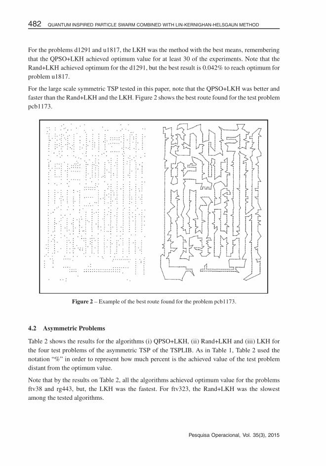
For the large scale symmetric TSP tested in this paper, note that the QPSO+LKH was better andfaster than the Rand+LKH and the LKH. Figure 2 shows the best route found for the test problempcb1173.

Figure 2 – Example of the best route found for the problem pcb1173.

4.2 Asymmetric Problems

Table 2 shows the results for the algorithms (i) QPSO+LKH, (ii) Rand+LKH and (iii) LKH forthe four test problems of the asymmetric TSP of the TSPLIB. As in Table 1, Table 2 used thenotation “%” in order to represent how much percent is the achieved value of the test problemdistant from the optimum value.

Note that by the results on Table 2, all the algorithms achieved optimum value for the problemsftv38 and rg443, but, the LKH was the fastest. For ftv323, the Rand+LKH was the slowestamong the tested algorithms.


�

�

“main” — 2016/1/12 — 17:36 — page 483 — #19�

�

�

�

�

�


Table 2 – Results of optimization of the instances for the asymmetric TSP.

InstanceMethod Minimum (%) Mean (%) Maximum (%) Median (%)

Standard deviation

(optimum) time(s)

ftv38 QPSO+LKH 1530 0.00 1532.00 0.13 1530.53 0.03 1530.00 0.00 0.90 0.1

(1530) Rand+LKH 1530 0.00 1532.00 0.13 1530.33 0.02 1530.00 0.00 0.76 0.1

LKH 1530 0.00 1532.00 0.13 1530.20 0.01 1530.00 0.00 0.61 ≈ 0

ftv170 QPSO+LKH 2755 0.00 2755.00 0.00 2755.00 0.00 2755.00 0.00 0.00 0.1

(2755) Rand+LKH 2755 0.00 2755.00 0.00 2755.00 0.00 2755.00 0.00 0.00 0.4

LKH 2755 0.00 2755.00 0.00 2755.00 0.00 2755.00 0.00 0.00 0.1

rg323 QPSO+LKH 1326 0.00 1327.73 0.13 1328.00 0.15 1328.00 0.15 0.70 29.1

(1326) Rand+LKH 1326 0.00 1327.33 0.10 1328.00 0.15 1328.00 0.15 0.98 24.9

LKH 1326 0.00 1327.07 0.08 1328.00 0.15 1328.00 0.15 1.03 20.2

rg443 QPSO+LKH 2720 0.00 2720.00 0.00 2720.00 0.00 2720.00 0.00 0.00 163

(2720) Rand+LKH 2720 0.00 2720.00 0.00 2720.00 0.00 2720.00 0.00 0.00 164

LKH 2720 0.00 2720.00 0.00 2720.00 0.00 2720.00 0.00 0.00 55

5 CONCLUSIONS AND FUTURE WORKS

The troubleshooting of the CO as, for example, the TSP, can be resolved by using recent ap-proaches such as particle swarm concepts and quantum mechanics. The metaheuristic QPSOis an optimization method based on the simulation of the social interaction among individualsin a population. Each element in it moves in a hyperspace, attracted by positions (promisingsolutions).

The LK heuristic is considered one of the most efficient methods for generating optimum ornear-optimum solutions for the symmetric TSP. However, the design and the execution of analgorithm based on this heuristic are not trivial. There are many possibilities for decision makingand most of them have a significant influence on the performance (Helsgaun, 2000).

As the Lin-Kernighan heuristic, the QPSO metaheuristic shows many parameters of settings andimplementations that directly affects the performance of the proposed algorithm. The algorithmshows promising results for the greater instances (n > 1000), range in which the LKH does notproduces such efficient results, even though it did not show satisfactory results for small instancesof the problem (n < 1000) (Nguyen et al., 2007).

New investigations can be done by varying the parameters of the QPSO algorithm and so adaptingthem to each of the instances to be tested. The size of the population, number of iterations andobviously, the LIP can vary. This probably would lead to an improvement of the performancesince each problem, even if the objective function is the same, show variations of behavior.There might be, for example, instances where clustering works well, as it is in the case of thealgorithm proposed by Neto (1999).


�

�

“main” — 2016/1/12 — 17:36 — page 484 — #20�

�

�

�

�

�


REFERENCES

[1] ALBAYRAK M & ALLAHVERDI N. 2011. Development a New Mutation Operator to Solve the

Traveling Salesman Problem by Aid of Genetic Algorithms. Expert Systems with Applications, 38:1313–1320.

[2] BAGHERI A, PEYHANI HM & AKBARI M. 2014. Financial Forecasting Using ANFIS Networks

with Quantum-behaved Particle Swarm Optimization. Expert Systems with Applications, 41: 6235–6250.

[3] BENIOFF P. 1980. The Computer as a Physical System: a Microscopic Quantum Mechanical Hamil-tonian Model of Computers as Represented by Turing Machines. Journal of Statistical Physics, 22:

563–591.

[4] CHEN SM & CHIEN CY. 2011. Parallelized Genetic Ant Colony Systems for Solving the TravelingSalesman Problem. Expert Systems with Applications, 38: 3873–3883.

[5] CHEN SM & CHIEN CY. 2011. Solving the Traveling Salesman Problem based on the Genetic Sim-

ulated Annealing and Colony System with Particle Swarm Optimization Techniques. Expert Systems

with Applications, 38: 14439–14450.

[6] CHRISTOFIDES N & EILON S. 1972. Algorithms for Large-scale Traveling Salesman Problems.Operational Research, 23: 511–518.

[7] CHUANG I & NIELSEN M. 2000. Quantum Computation and Quantum Information. Cambridge

University Press, Cambridge, England.

[8] COELHO LS & HERRERA BM. 2006. Fuzzy Modeling Using Chaotic Particle Swarm Approaches

Applied to a Yo-yo Motion System. Proceedings of IEEE International Conferenceon Fuzzy Systems,Vancouver, BC, Canada, pp. 10508–10513.

[9] COELHO LS. 2008. A Quantum Particle Swarm Optimizer with Chaotic Mutation Operator. Chaos,

Solutions and Fractals, 37: 1409–1418.

[10] CROES G. 1958. A Method for Solving Traveling Salesman Problems. Operations Research, 6:

791–8112.

[11] DONG G, GUO WW & TICKLE K. 2012. Solving the Traveling Salesman Problem using CooperativeGenetic Ant Systems. Expert Systems with Applications, 39: 5006–5011.

[12] FANG W, SUN J, DING Y, WU X & XU W. 2010. A Review of Quantum-behaved Particle Swarm

Optimization. IETE Technical Review, 27: 336–348.

[13] FEYMANN RP. 1982. Simulating Physics with Computers. International Journal of Theoretical

Physics, 21: 467–488.

[14] GROVER LK. 1996. A Fast Quantum Mechanical Algorithm for Database Search, Proceedings of the28th ACM Symposium on Theory of Computing (STOC), Philadelphia, PA, USA, pp. 212–219.

[15] HAMED HNA, KASABOV NK & SHAMSUDDIN SM. 2011. Quantum-Inspired Particle Swarm

Optimization for Feature Selection and Parameter Optimization in evolving Spiling Networks for

Classification Tasks. In: Evolucionary Algorithms (pp. 133–148). Croatia: Intech, 2011.

[16] HELSGAUN K. 2000. An Effective Implementation of the Lin-Kernighan Traveling Salesman Heuris-tic. European Journal of Operational Research, 126: 106–130.


�

�

“main” — 2016/1/12 — 17:36 — page 485 — #21�

�

�

�

�

�


[17] HERRERA BM & COELHO LS. 2006. Nonlinear Identification of a Yo-yo System Using Fuzzy

Model and Fast Particle Swarm Optimization. Applied Soft Computing Technologies: The Challenge

of Complexity, A. Abraham, B. de Baets, M. Koppen, B. Nickolay (editors), Springer, London, UK,

pp. 302–316.

[18] HOFFMANN KL. 2000. Combinatorial Optimization: Current Successes and Directions for the

Future. Journal of Computational and Applied Mathematics, 124: 341–360.

[19] HOGG T & PORTNOV DS. 2000. Quantum Optimization. Information Sciences, 128: 181–197.

[20] HOSSEINNEZHAD V, RAFIEE M, AHMADIAN M & AMELI MT. 2014. Species-based Quantum

Particle Swarm Optimization for Economic Load Dispatch. International Journal of Electrical

Power & Energy Systems, 63: 311–322.

[21] ISHIBUCHI H & MURATA T. 1998. Multi-objective Genetic Local Search Algorithm and its Ap-

plication to Flowshop Scheduling. IEEE Transactions on Systems, Man, and Cybernetics – Part C:

Applications and Reviews, 28: 392–403.

[22] JASZKIEWICZ A. 2002. Genetic Local Search for Multi-objective Combinatorial Optimization.

European Journal of Operational Research, 137: 50–71.

[23] JAU Y-M, SU K-L, WU C-J & JENG J-T. 2013. Modified Quantum-behaved Particle Swarm Op-

timization for Parameters Estimation of Generalized Nonlinear Multi-regressions Model Based onChoquet integral with Outliers. Applied Mathematics and Computation, 221: 282–295.

[24] JOHNSON DS. 1990. Local Optimization and the Traveling Salesman Problem. Lecture Notes in

Computer Science, 442: 446–461.

[25] JOHNSON DS & MCGEOCH LA. 1997. The Traveling Salesman Problem: A Case Study in Local

Optimization in: AARTS EHL & LENSTRA JK (eds.), Local Search in Combinatorial Optimization,John Wiley & Sons, INC, New York, NY, USA.

[26] KENNEDY J & EBERHART R. 1995. Particle Swarm Optimization. Proceedings of IEEE Interna-

tional Conference on Neural Networks, Perth, Australia, pp. 1942–1948.

[27] LAPORT G. 1992. The Traveling Salesman Problem: An overview of exact and approximate algo-rithms. European Journal of Operational Research, 59: 231–247.

[28] LAWLER EL, LENSTRA JK & SHMOYS DB. 1985. The traveling salesman problem: A guided tourof combinatorial optimization. Chichester: Wiley Series in Discrete Mathematics & Optimization.

[29] LI Y, JIAO L, SHANG R & STOLKIN R. 2015. Dynamic-context Cooperative Quantum-behaved

Particle Swarm Optimization Based on Multilevel Thresholding Applied to Medical Image Segmen-tation. Information Sciences, 294: 408–422.

[30] LIN L, GUO F, XIE X & LUO B. 2015. Novel Adaptive Hybrid Rule Network Based on TS FuzzyRules Using an Improved Quantum-behaved Particle Swarm Optimization. Neurocomputing, Part B,

149: 1003–1013.

[31] LIN S. 1965. Computer Solutions for the Traveling Salesman Problem. Bell Systems Technology

Journal, 44: 2245–2269.

[32] LIN S & KERNIGHAN BW. 1973. An Effective Heuristic Algorithm for the Traveling Salesman

Problem. Operations Research, 21: 498–516.


�

�

“main” — 2016/1/12 — 17:36 — page 486 — #22�

�

�

�

�

�


[33] LIU F & ZENG G. 2009. Study of Genetic Algorithm with Reinforcement Learning to Solve the TSP.

Expert Systems with Applications, 36: 6995–7001.

[34] LOPES HS & COELHO LS. 2005. Particle Swarm Optimization with Fast Local Search for the Blind

Traveling Salesman Problem. Proceedings of 5th International Conference on Hybrid Intelligent

Systems, Rio de Janeiro, RJ, pp. 245–250.

[35] LOURENCO HR, PAIXAO JP & PORTUGAL R. 2001. Multiobjective Metaheuristics for the Bus-

driver Scheduling Problem. Transportation Science, 35: 331–343.

[36] MACHADO TR & LOPES HS. 2005. A Hybrid Particle Swarm Optimization Model for the Trav-

eling Salesman Problem. H. Ribeiro, R. F. Albrecht, A. Dobnikar, Natural Computing Algorithms,Springer, New York, NY, USA, pp. 255–258.

[37] MANJU A & NIGAM MJ. 2014. Applications of Quantum Inspired Computational Intelligence: a

survey, Artificial Intelligence Review, 49: 79–156.

[38] MARIANI VC, DUCK ARK, GUERRA FA, COELHO LS & RAO RV. 2012. A Chaotic Quantum-behaved Particle Swarm Approach Applied to Optimization of Heat Exchangers. Applied Thermal

Engineering, 42: 119–128.

[39] MERZBACHER E. 1961. Quantum Mechanics. John Wiley & Sons, New York, NY, USA.

[40] MISEVICIUS A, SMOLINSKAS J & TOMKEVICIUS A. 2005. Iterated Tabu Search for the Traveling

Salesman Problem: new results. Information Technology and Control, 34: 327–337.

[41] MOSHEIOV G. 1994. The Traveling Salesman Problem with Pick-up and Delivery. European Journal

of Operational Research, 79: 299–310.

[42] NAGATA Y & SOLER D. 2012. A New Genetic Algorithm for the Asymmetric Traveling SalesmanProblem. Expert Systems with Applications, 39: 8947–8953.

[43] NEMHAUSER GL & WOLSEY AL. 1988. Integer and Combinatorial Optimization. John Wiley &

Sons, New York, NY, USA.

[44] NETO DM. 1999. Efficient Cluster Compensation for Lin-Kernighan Heuristics. PhD Thesis, Depart-

ment of Computer Science, University of Toronto, Canada.

[45] NGUYEN HD, YOSHIHARA I & YAMAMORI M. 2007. Implementation of an Effective Hybrid GAfor Large-Scale Traveling Salesman Problems. IEEE Transactions on System, Man, and Cybernetics-

Part B: Cybernetics, 37: 92–99.

[46] NGUYEN HD, YOSHIHARA I, YAMAMORI K & YASUNAGA M. 2006. Lin-Kernighan Variant. Link:http://public.research.att.com/˜dsj/chtsp/nguyen.txt

[47] PADBERG MW & RINALDI G. 1987. Optimization of a 532-city Symmetric Traveling SalesmanProblem by Branch and Cut. Operations Research Letters, 6: 1–7.

[48] PANG WJ, WANG KP, ZHOU CG & DONG LJ. 2004a. Fuzzy Discrete Particle Swarm Optimization

for Solving Traveling Salesman Problem. Proceedings of 4th International Conference on Computer

and Information Technology, Washington, DC, USA, pp. 796–800.

[49] PANG W, WANG KP, ZHOU CG, DONG LJ, LIU M, ZHANG HY & WANG JY. 2004b. Modi-fied Particle Swarm Optimization Based on Space Transformation for Solving Traveling Salesman

Problem. Proceedings of the 3rd International Conference on Machine Learning and Cybernetics, 4:2342–2346.


�

�

“main” — 2016/1/12 — 17:36 — page 487 — #23�

�

�

�

�

�


[50] PANG XF. 2005. Quantum Mechanics in Nonlinear Systems. World Scientific Publishing Company,

River Edge, NJ, USA.

[51] PAPADIMITRIOU CH & STEIGLITZ K. 1982. Combinatorial Optimization – Algorithms and Com-

plexity.Dover Publications, New York, NY, SA.

[52] POP PC, KARA I & MARC AH. 2012. New Mathematical Models of the Generalized Vehicle Rout-ing Problem and Extensions. Applied Mathematical Modelling, 36: 97–107.

[53] PURIS A, BELLO R & HERRERA F. 2010. Analysis of the Efficacy of a Two-Stage Methodology for

Ant Colony Optimization: Case of Study with TSP and QAP. Expert Systems with Applications, 37:

5443–5453.

[54] REINELT G. 1994. The Traveling Salesman: Computational Solutions for TSP Applications. Lecture

Notes in Computer Science, 840.

[55] ROBATI A, BARANI GA, POUR HNA, FADAEE MJ & ANARAKI JRP. 2012. Balanced Fuzzy Par-

ticle Swarm Optimization. Applied Mathematical Modelling, 36: 2169–2177.

[56] RYDNIK V. 1979. ABC’s of Quantum Mechanics. Peace Publishers, Moscow, U.R.S.S.

[57] SAUER JG, COELHO LS, MARIANI VC, MOURELLE LM & NEDJAH N. 2008. A Discrete Dif-

ferential Evolution Approach with Local Search for Traveling Salesman Problems. Proceedings of

the7th IEEE International Conference on Cybernetic Intelligent Systems, London, UK.

[58] SHANKAR R. 1994. Principles of Quantum Mechanics, 2nd Edition, Plenum Press.

[59] SHOR PW. 1994. Algorithms for Quantum Computation: Discrete Logarithms and Factoring, Pro-

ceedings of the35th Annual Symposim Foundations of Computer Science, Santa Fe, USA, pp. 124–

134.

[60] SHI Y, EBERHART R. 1999. Empirical study of particle swarm optimization. Proceedings of

Congress on Evolutionary Computation, Washington, DC, USA, pp. 1945–1950.

[61] SILVA CA, SOUSA JMC, RUNKLER TA & SA DA COSTA JMG. 2009. Distributed Supply Chain

Management using Ant Colony Optimization. European Journal of Operational Research, 199: 349–

358.

[62] SOSA NGM, GALVAO RD & GANDELMAN DA. 2007. Algoritmo de Busca Dispersa aplicado aoProblema Classico de Roteamento de Veıculos. Revista Pesquisa Operacional, 27(2): 293–310.

[63] STEINER MTA, ZAMBONI LVS, COSTA DMB, CARNIERI C & SILVA AL. 2000. O Problema de

Roteamento no Transporte Escolar. Revista Pesquisa Operacional, 20(1): 83–98.

[64] SUN J, FANG W, WU X, XIE Z & XU W. 2011. QoS Multicast Routing Using a Quantum-behaved

Particle Swarm Optimization Algorithm. Engineering Applications of Artificial Intelligence, 24:123–131.

[65] SUN J, FENG B & XU W. 2004a. Particle Swarm Optimization with Particles Having Quantum

Behavior. Proceedings of Congress on Evolutionary Computation, Portland, Oregon, USA, pp. 325–331.

[66] SUN J, FENG B & XU W. 2004b. A Global Search Strategy of Quantum-Behaved Particle SwarmOptimization. Proceedings of IEEE Congress on Cybernetics and Intelligent Systems, Singapore,

pp. 111–116.


�

�

“main” — 2016/1/12 — 17:36 — page 488 — #24�

�

�

�

�

�


[67] SUN J, XU W & FENG B. 2005a. Adaptive Parameter Control for Quantum-behaved Particle Swarm

Optimization on Individual Level. Proceedings of IEEE International Conference on Systems, Man

and Cybernetics, Big Island, HI, USA, pp. 3049–3054.

[68] SUN J, XU W & LIU J. 2005b. Parameter Selection of Quantum-Behaved Particle Swarm Optimiza-tion, International Conference Advances in Natural Computation (ICNC), Changsha, China, Lecture

Notes on Computer Science (LNCS) 3612, pp. 543–552.

[69] SUN J, XU W, PALADE V, FANG W, LAI C-H & XU W. 2012. Convergence Analysis and Improve-ments of Quantum-behaved Particle Swarm Optimization. Information Sciences, 193: 81–103.

[70] TASGERITEN MF & LIANG YC. 2003. A Binary Particle Swarm Optimization for Lot SizingProblem. Journal of Economic and Social Research, 5: 1–20.

[71] WANG KP, HUANG L, ZHOU CG, PANG CC & WEI P. 2003. Particle Swarm Optimization for

Traveling Salesman Problem. Proceedings of the 2nd International Conference on Machine Learning

and Cybernetics, Xi’an, China, pp. 1583–1585.

[72] WANG Y, FENG XY, HUANG YX, PU DB, LIANG CY & ZHOU WG. 2007. A novel quantum

swarm evolutionary algorithm and its applications. Neurocomputing, 70: 633–640.

[73] WILSON EO. 1971. The Insect Societies. Belknap Press of Harvard University Press, Cambridge,

MA.

[74] ZANG B, QI H, SUN S-C, EUAN L-M & TAN H-P. 2015. Solving Inverse Problems of Radiative

Heat Transfer and Phase Change in Semitransparent Medium by using Improved Quantum Particle

Swarm Optimization. International Journal of Heat and Mass Transfer, 85: 300–310.


Documents

Bruno Avila Leal de Meirelles Herrera , Leandro dos Santos ... · PDF file466 QUANTUM INSPIRED PARTICLE SWARM COMBINED WITH LIN-KERNIGHAN-HELSGAUN METHOD ... (Parallelized Genetic