The Science of Climate Change and Your Biology Class

Paul M. Beardsley, Ph.D.BSCS

Cal Poly Pomona, Center for Excellence in Mathematics and Science Teaching

The Challenge: 

• Earth’s climate is changing (…. the rates are not natural)• Public holds a myriad of ideas about Climate Science and impacts 

• Humans are making decisions for which outcomes won’t be realized for 30‐50 years  

• Learning about Climate Science relies on– principles of physics, chemistry, biology, earth sciences, and systems‐thinking that are tough

– students connecting concepts from different courses (e.g., expanding the Carbon Cycle in HS Biology)

– Do you currently teach about climate change? When in curriculum?

• Solutions are neither easy nor local, nor clearly connected to the field of climate science (….Energy). 

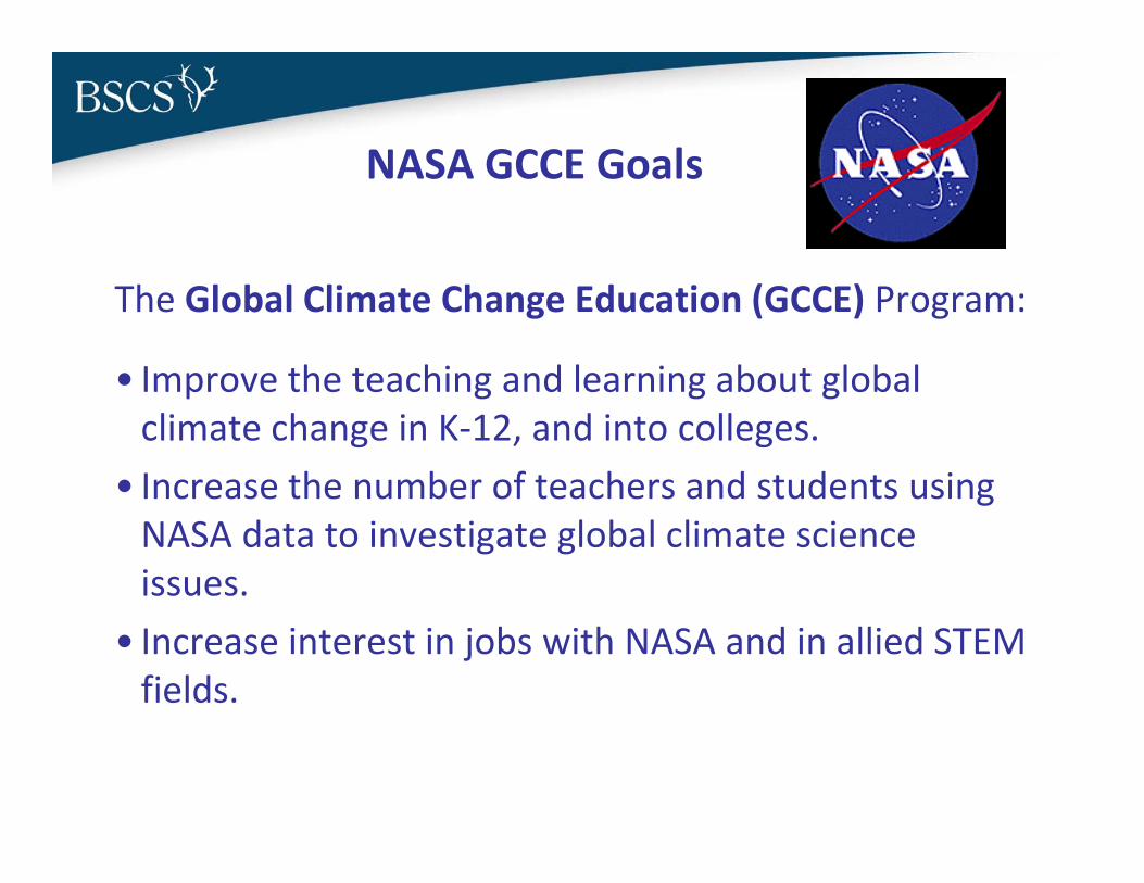
NASA GCCE Goals

The Global Climate Change Education (GCCE) Program: 

• Improve the teaching and learning about global climate change in K‐12, and into colleges. 

• Increase the number of teachers and students using NASA data to investigate global climate science issues. 

• Increase interest in jobs with NASA and in allied STEM fields. 

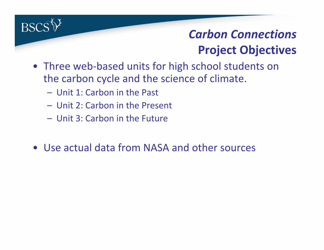
Carbon ConnectionsProject Objectives

• Three web‐based units for high school students on the carbon cycle and the science of climate.– Unit 1: Carbon in the Past– Unit 2: Carbon in the Present– Unit 3: Carbon in the Future  

• Use actual data from NASA and other sources

Carbon ConnectionsProject Objectives

• Improve students’ understanding of – carbon cycle and decision‐making for issues in climate  science,

– models and interactions of systems, – NASA’s role in monitoring Earth. 

• Increase student interest in careers at NASA and STEM fields.

• Goals for this session:– Make links in the Carbon Connections units to

biology courses– Have you experience and participate in using

some of the models and interactives from the field test version of Carbon Connections

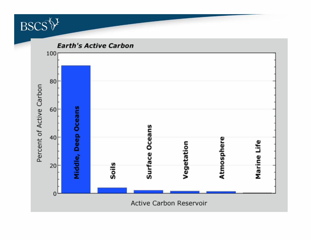
- Visualize flow of carbon among reservoirs- Scientists use evidence to infer climate

change on Earth - (emphasis on the past 650,000 years)

- Models can represent larger systems

Big Ideas for Unit 1:

• On your own, rank the following reservoirs of carbon in terms of their relative size:–Atmosphere–Deep, middle ocean–Terrestrial vegetation

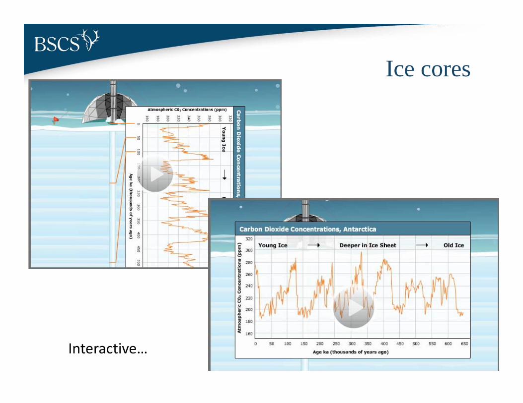
Ice cores

Interactive…

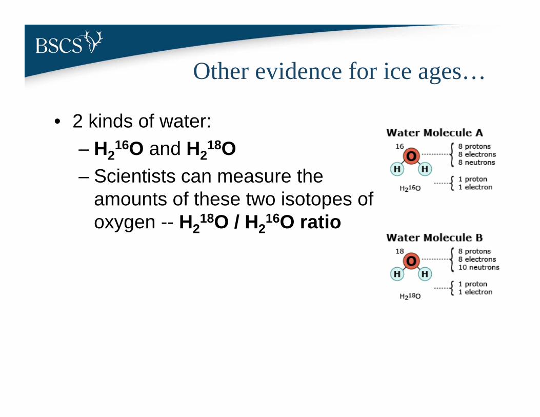
Other evidence for ice ages…

• 2 kinds of water:– H2

16O and H218O

– Scientists can measure the amounts of these two isotopes of oxygen -- H2

18O / H216O ratio

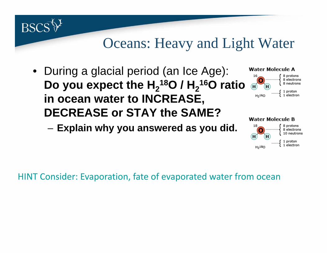
Oceans: Heavy and Light Water

• During a glacial period (an Ice Age): Do you expect the H2

18O / H216O ratio

in ocean water to INCREASE, DECREASE or STAY the SAME? – Explain why you answered as you did.

HINT Consider: Evaporation, fate of evaporated water from ocean

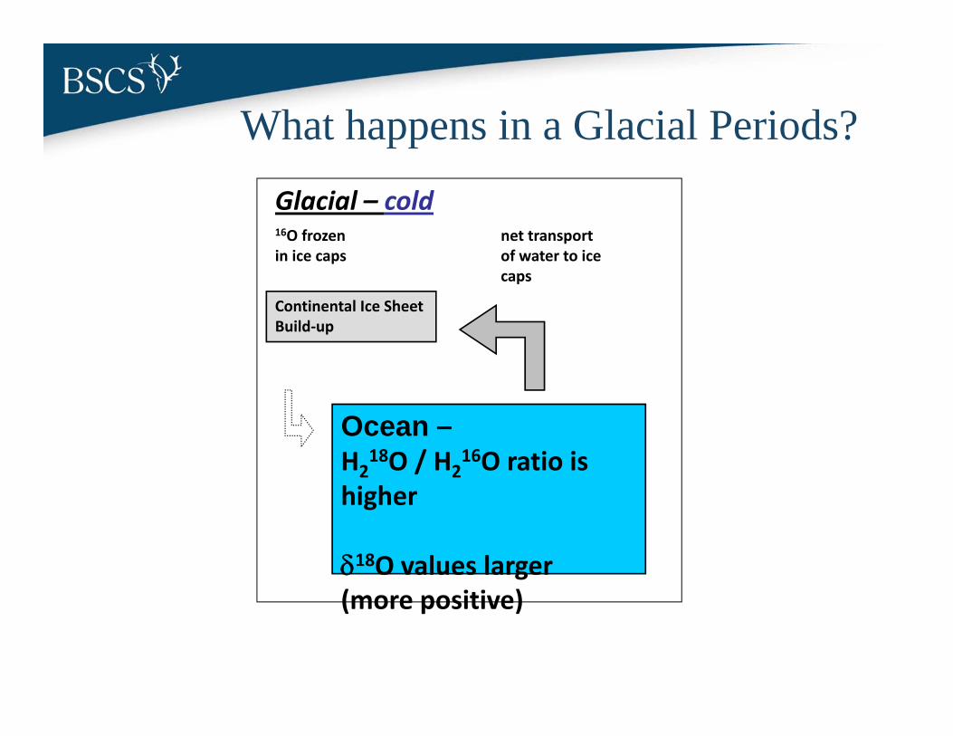
What happens in a Glacial Periods?Glacial – cold

Continental Ice Sheet Build‐up

Ocean –H2

18O / H216O ratio is 

higher

18O values larger (more positive)

16O frozen in ice caps

net transport of water to ice caps 

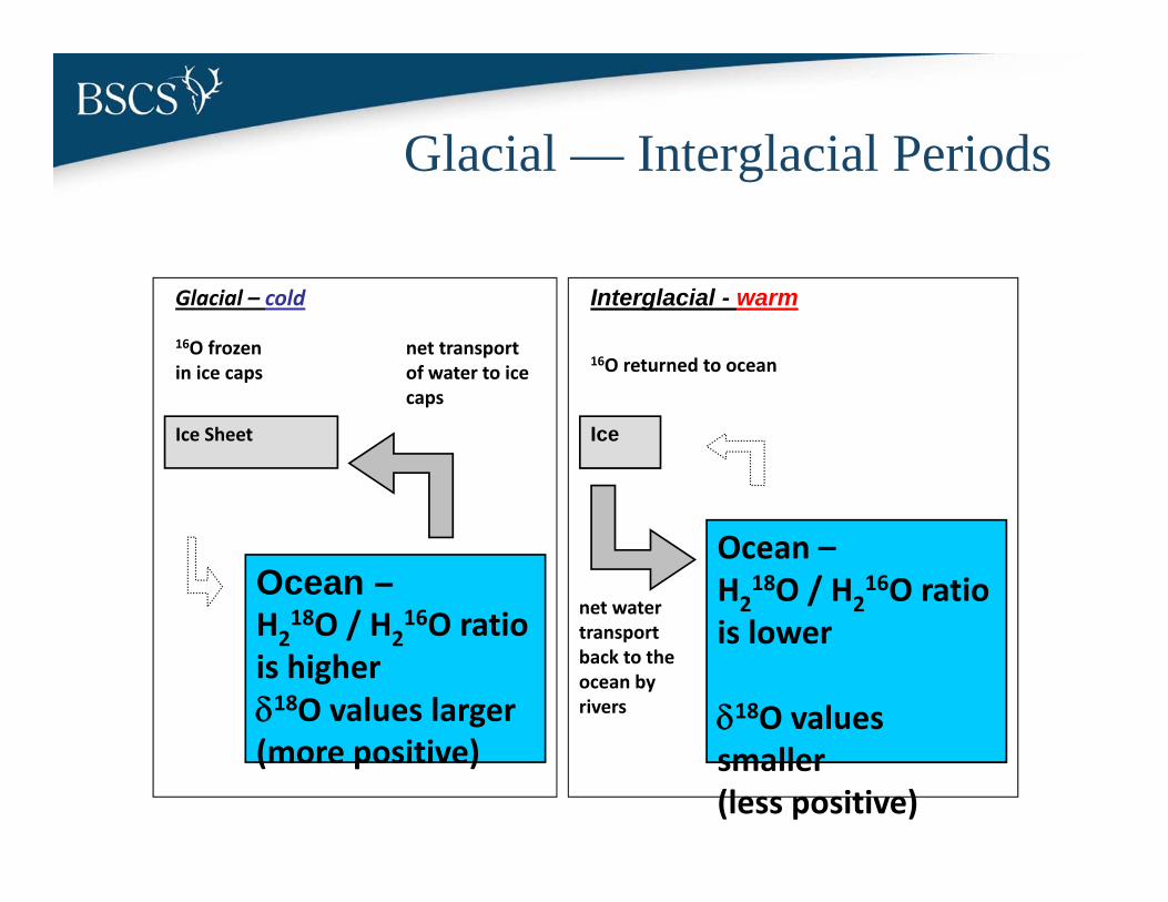
Glacial — Interglacial Periods

Glacial – cold Interglacial - warm

Ice Sheet Ice

Ocean –H2

18O / H216O ratio 

is higher18O values larger (more positive)

Ocean –H2

18O / H216O ratio 

is lower

18O values smaller (less positive)

16O frozen in ice caps

16O returned to oceannet transport of water to ice caps 

net water transport back to the ocean by rivers

Let’s Explore the Interactive…

Unit 1

• Students use interactive based on Global Climate Models to examine the relationship between CO2 and temperature– So called “spike experiments”

• Students also consider the movement of carbon among different reservoirs during glacial and interglacials– Time scales of tens of thousands of years

Unit 2 Carbon in the Present

• Students work to explain modern patterns of CO2 fluctuations using an understanding of living systems and movement of carbon among reservoirs

• Brief review of photosynthesis and respiration

Lesson 2.1

• Video from NASA shows the movement of CO2 across the world per month

• Students try to make sense, given what they think at this point

Watch video…

Lesson 2.2• Students reflect on the balance of

photosynthesis and respiration over a short time period

Lesson 2.2

• Students then apply what they learned to a larger system

Watch video…

Lesson 2.2 Sidetrip…

• As students consider the role of CO2 in living systems, they can choose to use NASA data to explore the impact of limiting factors on productivity

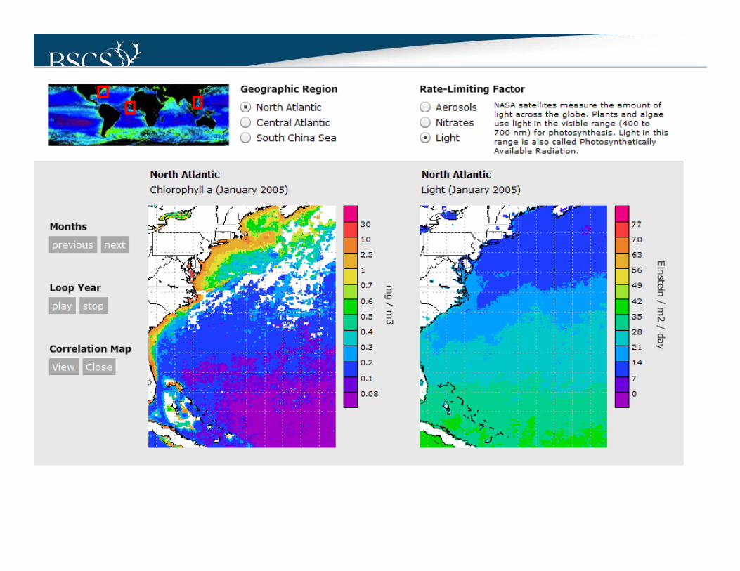
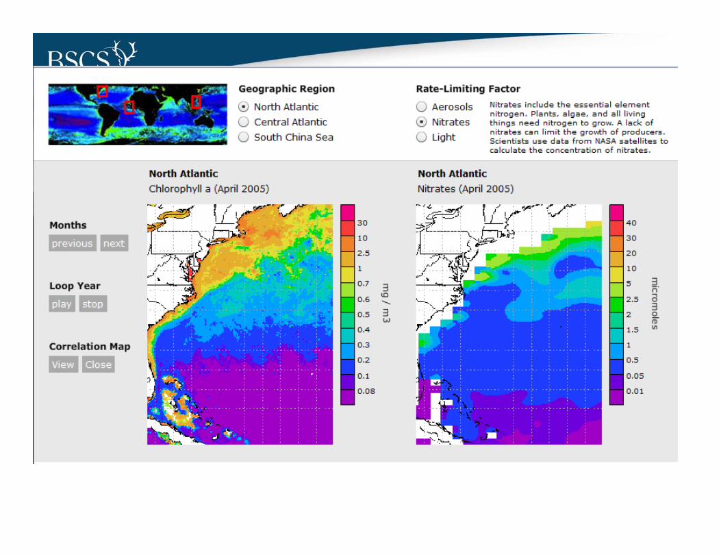
• Students explore the role of living systems in explaining patterns of carbon across the year

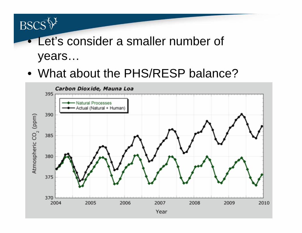
• Let’s consider a smaller number of years…

• What about the PHS/RESP balance?

• Let’s explore the interactive…– Not including the human component– Including the human component

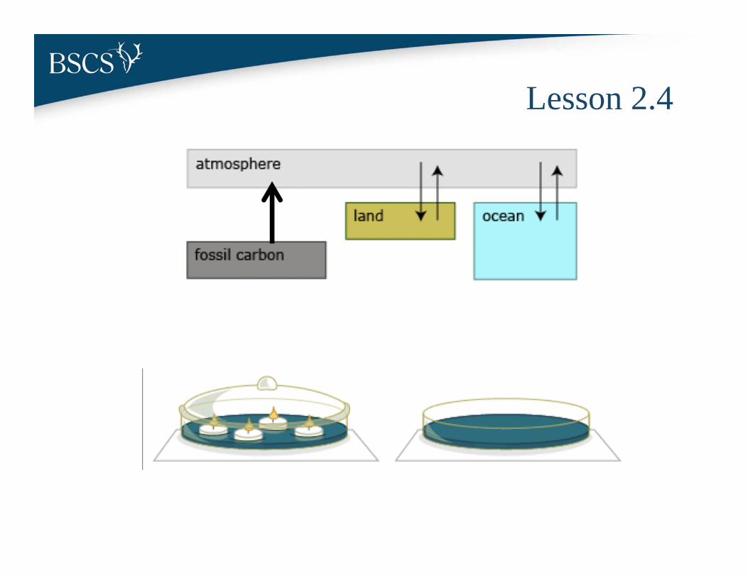
Lesson 2.4

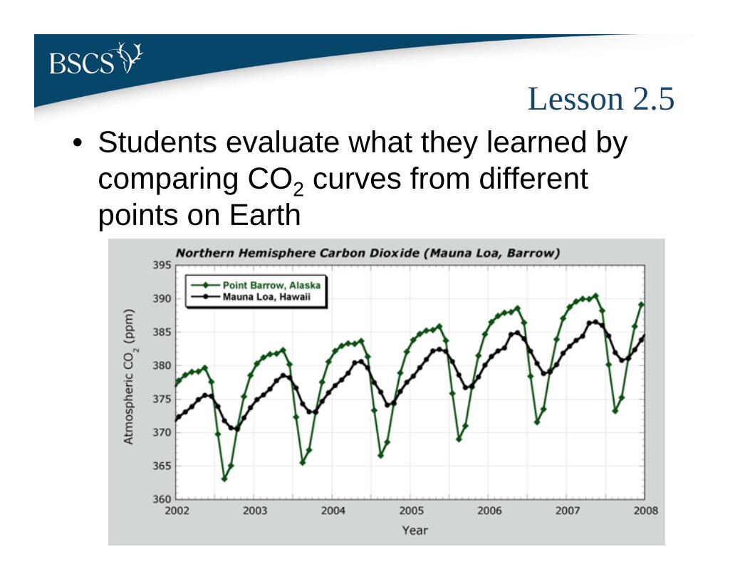
Lesson 2.5• Students evaluate what they learned by

comparing CO2 curves from different points on Earth

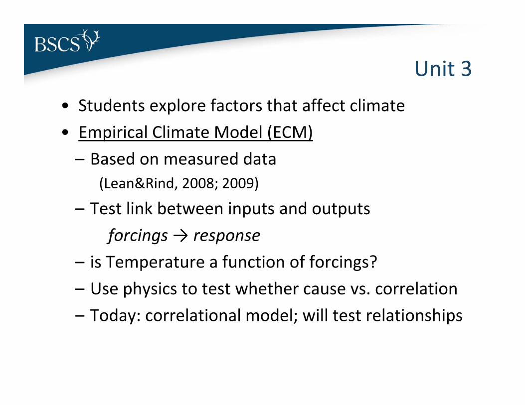
Unit 3• Students explore factors that affect climate• Empirical Climate Model (ECM)– Based on measured data

(Lean&Rind, 2008; 2009)

– Test link between inputs and outputs forcings→ response

– is Temperature a function of forcings?            – Use physics to test whether cause vs. correlation– Today: correlational model; will test relationships

The inputs:Forcing #1: El Niño/SO cycles  (ENSO)

-2.0

-1.0

0.0

1.0

2.0

3.0

4.0

1980 1985 1990 1995 2000 2005 2010

El Niño/La Niña Cycles (ENSO), 1979-2011

ENSO

Ind

ex

Year

El Niño events (peaks)

La Niña events (valleys)

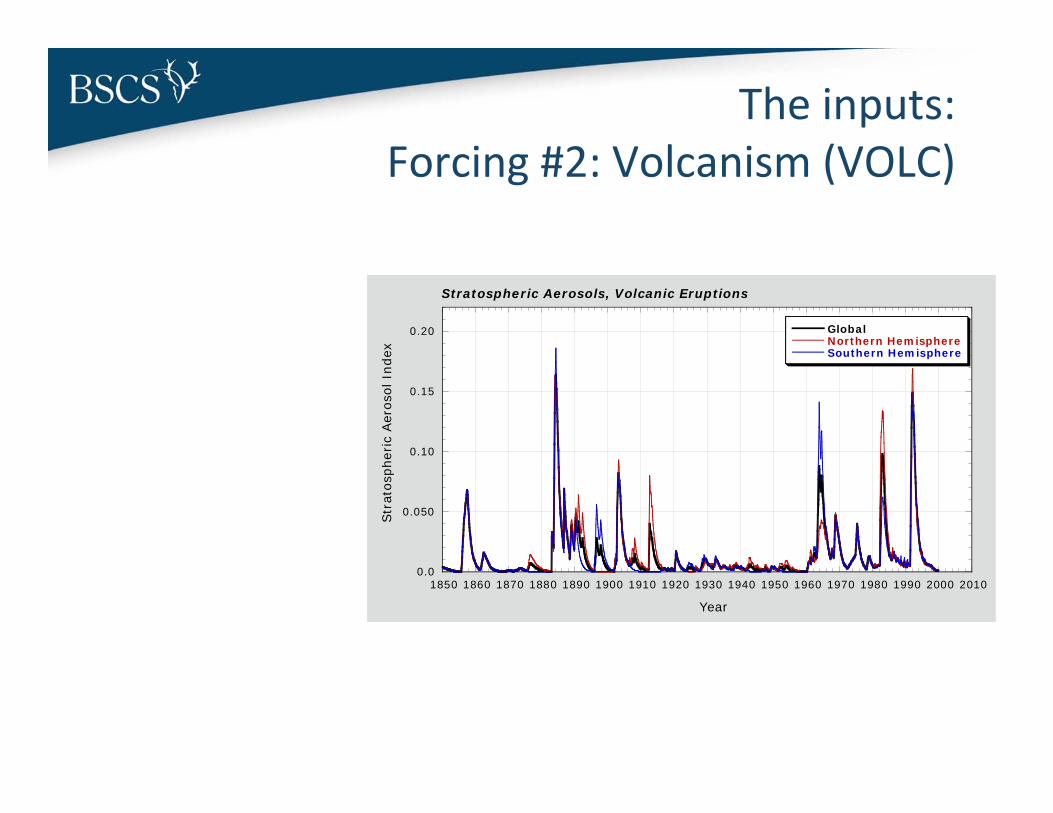
The inputs:Forcing #2: Volcanism (VOLC)

0.0

0.050

0.10

0.15

0.20

1850 1860 1870 1880 1890 1900 1910 1920 1930 1940 1950 1960 1970 1980 1990 2000 2010

Stratospheric Aerosols, Volcanic Eruptions

GlobalNorthern HemisphereSouthern Hemisphere

Stra

tosp

heric

Aer

osol

Ind

ex

Year

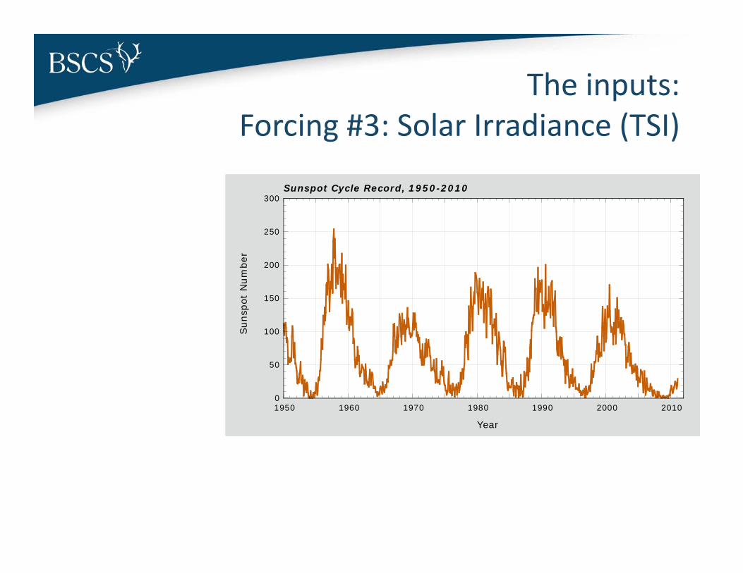
The inputs:Forcing #3: Solar Irradiance (TSI)

0

50

100

150

200

250

300

1950 1960 1970 1980 1990 2000 2010

Sunspot Cycle Record, 1950-2010

Sun

spot

Num

ber

Year

The inputs:Forcing #4: Human (ANTH)

• Green House Gas Emissions (GHGs)• Land use patterns• Tropospheric aerosols

• These have increased from 1979‐2010– Correlate with economic activity

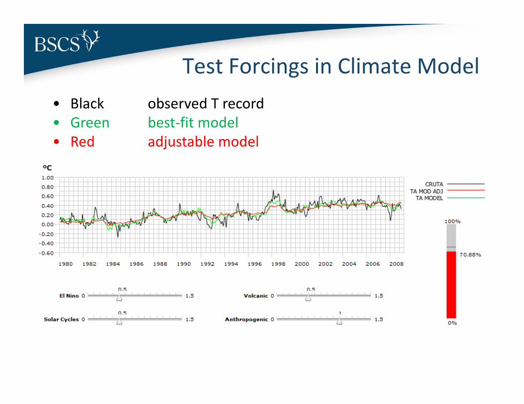
Test Forcings in Climate Model• Black observed T record• Green  best‐fit model• Red adjustable model

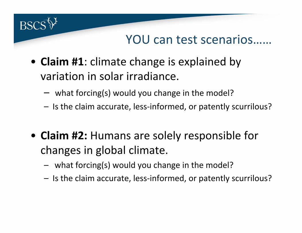
YOU can test scenarios……

• Claim #1: climate change is explained by variation in solar irradiance. – what forcing(s) would you change in the model?– Is the claim accurate, less‐informed, or patently scurrilous?

• Claim #2: Humans are solely responsible for changes in global climate. – what forcing(s) would you change in the model?– Is the claim accurate, less‐informed, or patently scurrilous? 

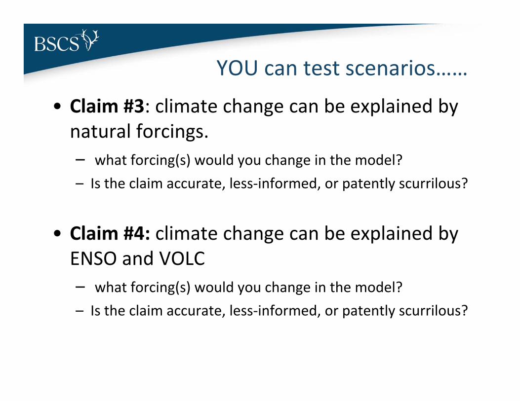
• Claim #3: climate change can be explained by natural forcings.  – what forcing(s) would you change in the model?– Is the claim accurate, less‐informed, or patently scurrilous?

• Claim #4: climate change can be explained by ENSO and VOLC– what forcing(s) would you change in the model?– Is the claim accurate, less‐informed, or patently scurrilous?

YOU can test scenarios……

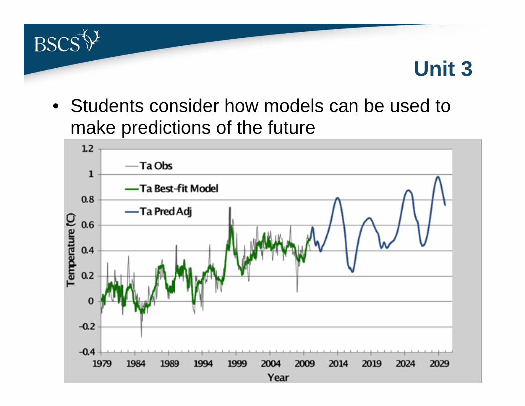
Unit 3• Students consider how models can be used to

make predictions of the future

Unit 3• Students go on to consider various ways they can

make a difference, through the use of carbon footprint analyses.

• Use footprint calculator from Nature Conservancy

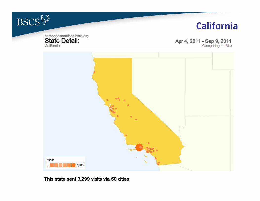
California

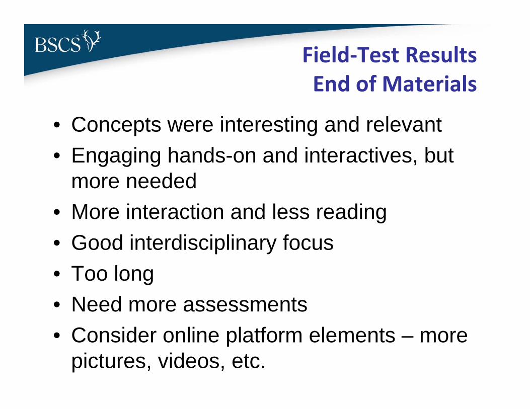
Field‐Test ResultsEnd of Materials

• Concepts were interesting and relevant• Engaging hands-on and interactives, but

more needed • More interaction and less reading• Good interdisciplinary focus• Too long• Need more assessments• Consider online platform elements – more

pictures, videos, etc.

Second Field Test Opportunity

• You can explore the student web materialshttp://carbonconnections.bscs.org/curriculum/

• Mid February– participate in the field test!• Contact Steve Getty:

sgetty@bscs.org