BSSRDF Explorer: A renderingframework for the BSSRDF

Benedikt Bitterli

Bachelor ThesisApril 2013

Supervisor:Prof. Markus Gross

Advisors:Dr. Wojciech Jarosz

Dr. Ralf Habel

Eidgenössische Technische Hochschule ZürichSwiss Federal Institute of Technology Zurich

Abstract

This thesis introduces a novel system for the development, display and analysis of bidirectionalsurface scattering distribution functions (BSSRDFs). The system is capable of interactively ren-dering analytic BSSRDFs on arbitrary triangle meshes and pointclouds under different lightingconditions. It also facilitates analysis and validation of BSSRDFs by providing comparisonplots both for analytic BSSRDFs and measured data in form of radial profiles. Additionally, thesystem provides reference solutions by the means of path tracing for simple geometries. Thesystem is easily extensible with new analytic BSSRDFs through a simple text file interface. Forthe BSSRDF, our system is the first of its kind and is targeted both at researchers to assist indevelopment and survey of BSSRDFs as well as artists to allow for interactive feedback andincreased control in tweaking BSSRDF parameters. We integrated our system with the popularBRDF Explorer from Walt Disney Animation Studios and release it as an open source applica-tion to the computer graphics community.

i

Zusammenfassung

Diese Arbeit führt ein neues System für die Entwicklung, Darstellung and Analyse von Bidi-rectional Surface Scattering Distribution Functions (BSSRDFs) ein. Das System unterstütztdie interaktive Darstellung von BSSRDFs auf beliebigen Dreiecksmodellen und Punktwolkenunter verschiedenen Lichtverhältnissen. Es vereinfacht ausserdem die Analyse und Validierungvon BSSRDFs durch das Bereitstellen von Vergleichsgraphen für analytische BSSRDFs undgemessene Daten in Form von radialen Profilen. Zusätzlich stellt das System Referenzlösungenauf einfachen Geometrien bereit, die mithilfe von Path Tracing berechnet werden. Das Systemkann leicht mit neuen analytischen BSSRDFs erweitert werden. Unser System ist das erste ver-gleichbare System für die BSSRDF und richtet sich sowohl an Forscher, um die Entwicklungund Studie von BSSRDFs zu unterstützen, als auch an Künstler, um das Finden von passendenBSSRDF-Parametern durch interaktives Feedback zu vereinfachen. Unser System basiert aufdem bekannten BRDF Explorer von Walt Disney Animation Studios und wird als Open SourceAnwendung veröffentlicht.

iii

Prof. Markus Gross

Bachelor’s Thesis

BSSRDF Editing in BRDF Explorer

Introduction

The goal of this bachelor thesis is to implement GPU based BSSRDF (Bidirectional Subsurface Scattering Reflection Distribution Function) editing and display capabilities into the open source BRDF Explorer application from Walt Disney Animation Studios. This will allow the assessment of established and novel BSSRDF models and the editing of BSSRDF parameters in a feature production environment. To achieve this goal, the existing BRDF Explorer application needs to be extended and an interface to GLSL BSSRDFs is to be defined within the BRDF Explorer framework. All standard BSSRDF models such as Dipole and Quantized Diffusion under different boundary conditions are then implemented in this interface.

Tasks Orientation, review of related work. Reviewing BRDF Explorer code base Definition of BSSRDF interface in BRDF Explorer

- Assessment of effectivity and generality of interface Implementation of UI plots of BSSRDF values Implementation of Dipole and Quantized Diffusion

With these tasks fulfilled, the grade is 4.00

Implementing ray tracing capabilities into BRDF Explorer viewport With these tasks fulfilled, the grade is 5.00

Implementation of a simple GPU based volumetric path tracer for BSSRDF reference. Implementation of rapid-hierarchical subsurface scattering on the GPU .

With these tasks fulfilled, the grade is 6.00

Dates Start Date: Thursday, November 1, 2012 - Thursday, April 30, 2012

Acknowledgements

I would like to express my gratitude to my advisors, Wojciech Jarosz and Ralf Habel, for devot-ing their precious time to my questions and their guidance throughout this project. Furthermore,I would like to thank Brent Burley for his feedback and support and enabling this thesis in thefirst place. Thanks also go to Marios Papas for his interest and insight. I am also deeply gratefulto my family for their unconditional support and encouragement.

vii

Contents

List of Figures x

List of Algorithms xiii

1. Introduction 11.1. Related Work . . . . . . . . . . . . . . . . . . . . . . . . . . . . . . . . . . . 2

2. Background 52.1. Surface Scattering . . . . . . . . . . . . . . . . . . . . . . . . . . . . . . . . . 52.2. Volumetric Scattering . . . . . . . . . . . . . . . . . . . . . . . . . . . . . . . 62.3. The Searchlight Problem . . . . . . . . . . . . . . . . . . . . . . . . . . . . . 92.4. Diffusion Theory . . . . . . . . . . . . . . . . . . . . . . . . . . . . . . . . . 102.5. The Diffusion Dipole . . . . . . . . . . . . . . . . . . . . . . . . . . . . . . . 132.6. Rendering with the BSSRDF . . . . . . . . . . . . . . . . . . . . . . . . . . . 14

2.6.1. Reduced Radiance . . . . . . . . . . . . . . . . . . . . . . . . . . . . 142.6.2. Single Scattering . . . . . . . . . . . . . . . . . . . . . . . . . . . . . 152.6.3. Monte Carlo Multiple Scattering Evaluation . . . . . . . . . . . . . . . 162.6.4. Hierarchical Multiple Scattering Evaluation . . . . . . . . . . . . . . . 17

3. Implementation 213.1. System Overview . . . . . . . . . . . . . . . . . . . . . . . . . . . . . . . . . 21

3.1.1. Parameter Module . . . . . . . . . . . . . . . . . . . . . . . . . . . . 213.1.2. Point Cloud Module . . . . . . . . . . . . . . . . . . . . . . . . . . . 223.1.3. Lit Sphere Modules . . . . . . . . . . . . . . . . . . . . . . . . . . . . 223.1.4. Pencil Beam Module . . . . . . . . . . . . . . . . . . . . . . . . . . . 22

3.2. Volumetric Path Tracing . . . . . . . . . . . . . . . . . . . . . . . . . . . . . 24

ix

Contents

3.3. Rendering Translucency . . . . . . . . . . . . . . . . . . . . . . . . . . . . . 263.3.1. Point Cloud Generation . . . . . . . . . . . . . . . . . . . . . . . . . 273.3.2. Irradiance Computation . . . . . . . . . . . . . . . . . . . . . . . . . 273.3.3. Radiance Evaluation . . . . . . . . . . . . . . . . . . . . . . . . . . . 29

3.4. Parameter Inversion . . . . . . . . . . . . . . . . . . . . . . . . . . . . . . . . 313.5. BSSRDF Integration on the Sphere . . . . . . . . . . . . . . . . . . . . . . . . 333.6. User Interface . . . . . . . . . . . . . . . . . . . . . . . . . . . . . . . . . . . 35

3.6.1. Parameter Window . . . . . . . . . . . . . . . . . . . . . . . . . . . . 353.6.2. Lit Sphere Widgets . . . . . . . . . . . . . . . . . . . . . . . . . . . . 363.6.3. Pencil Plot Widget . . . . . . . . . . . . . . . . . . . . . . . . . . . . 373.6.4. Point Cloud Widget . . . . . . . . . . . . . . . . . . . . . . . . . . . . 39

4. Conclusion and Future Work 41

A. Appendix 43A.1. Efficient Pseudorandom Float Generation . . . . . . . . . . . . . . . . . . . . 43A.2. BSSRDF Interface . . . . . . . . . . . . . . . . . . . . . . . . . . . . . . . . 45

Bibliography 48

x

List of Figures

2.1. Light scattering model for (a) BRDF and (b) BSSRDF. Figure reproduced fromJensen et al. [JMLH01] . . . . . . . . . . . . . . . . . . . . . . . . . . . . . . 6

2.2. The behaviour of light in a participating medium is characterized by four differ-ent interactions: (a) absorption, (b) emission, (c) outscattering and (d) inscat-tering. Figure reproduced from Jarosz [Jar08] . . . . . . . . . . . . . . . . . . 7

2.3. Outline of the searchlight problem . . . . . . . . . . . . . . . . . . . . . . . . 92.4. The dipole setup . . . . . . . . . . . . . . . . . . . . . . . . . . . . . . . . . . 142.5. Evaluation of (a) reduced radiance and (b) single scattering . . . . . . . . . . . 152.6. Monte Carlo integration of the multiple scattering term requires sampling both

surface area and light sources. Figure reproduced from [JMLH01] . . . . . . . 162.7. Hierarchical pointcloud evaluation uses irradiance values at precomputed sur-

face locations and may cluster distant samples . . . . . . . . . . . . . . . . . . 172.8. Results for 10 iterations (top), 100 iterations (middle) and 1000 iterations (bot-

tom) of the point relaxation algorithm, rendered with the dipole BSSRDF (left,middle) and visualized directly (right). Model courtesy of XYZRGB. . . . . . 18

2.9. Benefits of BSSRDF evaluation with sample clustering compared to evaluationwithout sample clustering, illustrated on a pointcloud with 100′000 samples,rendered at 1680× 1050 pixels. With sample clustering (a), rendered in 140ms;without sample clustering and equal number of samples (b) rendered in 8.5seconds; no sample clustering and equal render time (140ms) (c) allows only400 samples. Note that (a) is visually equivalent to (b), despite being 60 timesfaster. Model courtesy of the Stanford Computer Graphics Laboratory. . . . . . 19

xi

List of Figures

3.1. Summary of different lighting modes supported by the point cloud module: di-rectional (a), filtered directional (here with checker texture) (b), IBL (c) andoccluded IBL (d). Top: Irradiance samples. Bottom: Rendered with dipoleBSSRDF. Model courtesy of XYZRGB. Environment map courtesy of Paul De-bevec. . . . . . . . . . . . . . . . . . . . . . . . . . . . . . . . . . . . . . . . 23

3.2. Sample set subdivision for octree construction . . . . . . . . . . . . . . . . . . 263.3. Results for different shadow mapping methods: naive (a), with offset (b), with

offset and hardware PCF (c) and with offset, hardware PCF and multiple jitteredlookups (d). Model courtesy of the Stanford Computer Graphics Laboratory. . . 28

3.4. Layout of the descriptor arrays. Top: Example octree. Middle: Child descriptorarray. Bottom: Point sample array. Not shown: Node attribute arrays . . . . . . 30

3.5. 32bit child descriptor . . . . . . . . . . . . . . . . . . . . . . . . . . . . . . . 303.6. User interface. Model courtesy of the Stanford Computer Graphics Laboratory. 353.7. Overview of the parameter window (split up into columns) . . . . . . . . . . . 363.8. Influence of the scale parameter on the rendered image: Values of 10 (a), 50

(b), 200 (c) and 500 (d) for the dipole BSSRDF, from the front (top) and back(bottom). Model courtesy of the Stanford Computer Graphics Laboratory. . . . 37

3.9. Overview of the lit sphere widgets . . . . . . . . . . . . . . . . . . . . . . . . 383.10. Overview of the pencil plot widget . . . . . . . . . . . . . . . . . . . . . . . . 39

A.1. IEEE Float representation . . . . . . . . . . . . . . . . . . . . . . . . . . . . . 44

xii

List of Algorithms

1. Volumetric path tracing . . . . . . . . . . . . . . . . . . . . . . . . . . . . . . 252. Octree traversal . . . . . . . . . . . . . . . . . . . . . . . . . . . . . . . . . . 32

xiii

1Introduction

Realistic rendering of translucent materials poses a challenging problem in computer graphics.Many materials important for realistic image synthesis, such as plants and fruits, beverages andfood, many liquids and even our own skin, exhibit strong subsurface scattering effects. Tradi-tionally, these effects have been approximated using models describing purely reflective lighttransport, commonly summarized in bidirectional reflectance distribution functions (BRDFs).However, the BRDF only describes scattering at a single point and fails to model light transportwithin the medium between different points on the surface. To properly account for subsurfacelight transport, a generalization of the BRDF, the bidirectional surface scattering distributionfunction (BSSRDF), can be used. The BSSRDF describes light transport between any two raysthat hit a surface, enabling the incorporation of subsurface light transport.

Recent developments, such as the introduction of diffusion theory [Sta95] and the diffusiondipole [JMLH01] to computer graphics, have laid the foundation for many practical subsurfacelight tranport models and spawned numerous novel BSSRDFs. Sophisticated rendering tech-niques and increase in computational power have also made it feasible to incorporate subsurfacescattering effects into movie production, sparking interest in finding and developing BSSRDFsoptimal in artist workflow and visual quality.

At this point, a wealth of different BRDF and BSSRDF models exist. For the BRDF, severalsystems [Rus01, FPBP09, Stu11] address the problem of development, analysis and survey ofanalytic and measured models. Additionally, some of them [FPBP09, Stu11] provide GPUbased rendering capabilities, allowing interactive visual feedback for a wide range of parametersettings and lighting conditions.

So far, no such system exists for the BSSRDF. In addition, the BSSRDF is inherently more ex-pensive to render than the BRDF, making the implementation of accurate interactive renderingmethods difficult. However, fast visual feedback when editing the parameters of a BRDF or

1

1. Introduction

BSSRDF is vital to the workflow of an artist.

The contributions of this thesis are as follows:

• Introduction of an extensible system supporting the development, analysis and validationof new and existing BSSRDFs

• Implementation of BSSRDFs widely used in research and production in our system

• GPU implementations of state-of-the-art BSSRDF rendering methods, allowing interac-tive display and interaction with BSSRDFs

A table of notation used throughout this paper is given in table 1.1.

1.1. Related Work

Several rendering algorithms, such as path tracing [Kaj86] or photon mapping [Jen01] addressthe problem of numerically approximating volumetric scattering effects. Although these meth-ods are general in that they can handle arbitrary illumination, geometry and materials in anunbiased manner, they are typically computationally expensive and may take long to converge,making them infeasible for practical rendering.

The diffusion approximation introduced to computer graphics by Stam [Sta95] approximatesmultiple scattering using a diffusion equation and forms the basis for many successful BSS-RDFs. Building on work from classical diffusion theory [FPW92], Jensen et al. [JMLH01]introduce a practical diffusion dipole model. Combined with a single scattering term based onwork by Hanrahan and Krueger [HK93], they build a BSSRDF and apply it to the rendering oftranslucent materials. Donner and Jensen [DJ05] extend this work with a multipole and use itto render multi-layered materials. d’Eon and Irving [DI11], among a wealth of improvementsupon classic diffusion theory, also introduce a new diffuse multiple scattering term built from asum of Gaussians.

Several methods attempt to render subsurface scattering effects interactively. d’Eon et al.[dL07] and Jimenez et al. [JWSG10] both approximate subsurface scattering by approximatingthe diffusion profile by a sum of Gaussians and exploit separability to blur the illumination intexture space. Subsequent work by Jimenez and Gutierrez [JG10] is based on the same observa-tion, but performs the blur in screen-space, increasing performance at the cost of quality. Whilethese techniques work in real-time, they focus on skin rendering and don’t allow for generalBSSRDFs. Jensen and Buhler [JB02] introduce a two-pass rendering technique to significantlyimprove performance when evaluating the BSSRDF on general geometry. Although originallyintended for use with the diffusion dipole for offline rendering, it is also applicable to generalBSSRDFs and is suitable for interactive GPU rendering.

Multiple applications focusing on visualization, analysis and manipulation of BRDFs exist.bv [Rus01] features several analytic BRDFs in lit-sphere and goniometric views. BRDFLab[FPBP09] allows visualization of BRDFs on different geometry and lighting situations andfeatures parameter fitting and BRDF synthesis. The BRDF Explorer by Walt Disney AnimationStudios [Stu11] provides an extensible, GPU based system for BRDFs under different lighting

2

1.1. Related Work

conditions and arbitrary geometry as well as analysis facilities. Our system is based on the opensource BRDF Explorer and uses its extensible GPU framework to allow dynamic loading andediting of analytic BSSRDFs.

3

1. Introduction

Symbol Description

~xi Surface location of incident light~ωi Incident direction~xo Surface location of exitant light~ωo Exitant direction~n Surface normalfr BRDFft BTDFS BSSRDFS(0) Reduced radianceS(1) Single scattered radianceSd Multiple scattered radianceL RadianceLr Reflected radianceLi Incident radianceEi IrradianceΦi Incident fluxD Diffusion constantφ Fluence~E Fluxp Phase functiong Mean cosine of scattering angleσa Absorption coefficientσs Scattering coefficientσ′s Reduced scattering coefficient: (1− g)σsσt Extinction coefficient: σs + σaσ′t Reduced extinction coefficient: σ′s + σaα Albedo: σs/σtα′ Reduced albedo: σ′s/σtσtr Effective transport coefficient:

√σa/D

Q Source functionη Relative index of refractionFr Fresnel reflectanceFt Fresnel transmittanceFdr Average Fresnel reflectancel Mean free path (mfp): 1/σtl′ Reduced mean free path: 1/σ′tld Diffuse mean free path (dmfp): 1/σtrRd Diffuse reflectanceΩ+ Hemisphere of outward directionsΩ− Hemisphere of inward directionsΩ Domain of integration

Table 1.1.: Table of notation

4

2Background

Fundamental to realistic image synthesis is the concept of light transport. It describes the be-haviour of light as it is emitted from light sources, interacts with the scene and ultimately arrivesat the camera, producing the rendered image. Accurately modeling the light transport is key forsynthesizing realistic images. Unfortunately, the physical behaviour of light is complex and notcompletely understood, necessitating simplifying assumptions to allow for efficient simulation.

2.1. Surface Scattering

Most light phenomena can be described accurately using the model of geometric optics. It isbased on the assumption that light propagates with infinite speed along straight lines (rays).Light rays may only change direction at a discrete set of scattering locations, at which theirrespective energies may be partially absorbed and the remaining fraction scattered into newdirections. Importantly, it is assumed that radiance along a ray is constant; the medium throughwhich the ray travels does not influence the light transport.

For most applications, it is a reasonable approximation to restrict the location of scatteringevents to only the surface of objects. In this model, rays of light travel without scattering untilthey strike the surface of an object, at which point they are either absorbed completely or scatterand leave the surface at the same location in new directions. This gives rise to the notion of thebidirectional reflectance distribution function (BRDF) introduced by Nicodemus [NRH+77],which, for a ray coming from direction ~ωi striking a surface at location xi, relates the incomingradiance Li to the reflected radiance Lr:

5

2. Background

(a) (b)

Figure 2.1.: Light scattering model for (a) BRDF and (b) BSSRDF. Figure reproduced from Jensen etal. [JMLH01]

fr(~x, ~ωi, ~ωo) =dLr(~x, ~ωo)

dEi(~x, ~ωi)=

dLr(~x, ~ωo)

Li(~x, ~ωi)(~ωi·~n)d~ωi, (2.1)

where ~n is the surface normal.

If the incident radiance field Li is known for all directions, the total reflected radiance Lr indirection ~ωo can be obtained by integration:

Lr(~x, ~ωo) =

∫Ω

fr(~x, ~ωi, ~ωo)dEi(~x, ~ωi) =

∫Ω

fr(~x, ~ωi, ~ωo)Li(~x, ~ωi)(~ωi·~n)d~ωi (2.2)

Here, Ω represents the hemisphere of incident directions at location ~x.

However, for the description of volumetric scattering, these approximations are not sufficient.Several problems arise when dealing with materials that exhibit volumetric scattering - mostimportantly, the assumption of constant radiance along a ray does no longer hold. The mediumin which the ray travels now does influence the light transport; it is thus commonly referredto as a participating medium. In addition, scattering events happen not only on the surface ofobjects, but volumetrically within the medium.

2.2. Volumetric Scattering

To properly predict the behaviour of light as it moves through a participating medium, we needan extended model accounting for volumetric scattering. In reality, volumetric scattering iscaused by particles suspended in the medium (air molecules, dust, pigments, microorganismsetc.). Light travelling through the medium hits these particles and interacts with them on amicroscopic level.

Actually modelling the particles and individual interactions with light is impractical and unnec-essary for most rendering applications. However, if we assume the particles to be microscopic(much smaller than the spacing between particles) and randomly positioned, we can insteadonly model the probabilistic behaviour of light moving through the medium, aggregated overmany interactions with particles.

6

2.2. Volumetric Scattering

(a)(b) (c) (d)

Figure 2.2.: The behaviour of light in a participating medium is characterized by four different interac-tions: (a) absorption, (b) emission, (c) outscattering and (d) inscattering. Figure reproducedfrom Jarosz [Jar08]

Specifically, we now consider the radiance along an infinitesimal ray of light moving throughthe medium by describing the change in radiance after an infinitesimal step along the ray. Thechange is characterized by the current position along the ray ~x, the direction of the ray ~ω andthe radiance L(~x, ~ω). Since we are assuming infinitesimal steps, we consider the differentialchange (~ω · ∇)L(~x, ~ω).

For each such infinitesimal step, we model four possible interactions with the medium, illus-trated in Figure 2.2:

Absorption Part of the radiance is absorbed by the medium. Since all interactions conserveenergy, the radiance doesn’t vanish; instead, it is converted into different forms of energy, suchas heat. For our purposes, we can simply consider the radiance to have vanished with absorption,since other forms of energy are invisible to the human eye. The absorbed fraction of the radianceis described by the absorption coefficient σa. Putting it in differential form describes the changein radiance as:

(~ω · ∇)L(~x, ~ω) = −σaL(~x, ~ω) (2.3)

Emission In some cases, the medium itself may produce light. Chemical reactions, foundin burning gases for example, may cause volumetric emission within the medium; in fact, thesunlight that we see daily is produced by self-emission within the sun, caused by fission reac-tion. Although not necessarily physically plausible, volumetric emission is also of interest incomputer animation, leaving many possibilities to the artist for visual effects. In general, wecan model emission within the medium using a source term Q(~x, ~ω), dependent on location anddirection. In differential form:

(~ω · ∇)L(~x, ~ω) = Q(~x, ~ω) (2.4)

Outscattering At each step, the radiance may also be reduced due to light being scatteredinto other directions than ~ω. The fraction of radiance being scattered is described by the scat-tering coefficient σs. Similar to the absorption, we can formulate it in differential form as:

(~ω · ∇)L(~x, ~ω) = −σsL(~x, ~ω) (2.5)

7

2. Background

Inscattering Finally, we also have to take into account the radiance arriving at ~x from otherdirections and being scattered towards direction ~ω, increasing the radiance along the ray. Again,we use the scattering coefficient σs to describe the fraction of radiance being scattered. Addi-tionally, capturing all incident directions means integrating the incident radiance over the wholesphere of directions Ω:

(~ω · ∇)L(~x, ~ω) =

∫Ω

p(~ω′, ~ω)L(~x, ~ω′)d~ω′ (2.6)

Here, we used the phase function p. The phase function describes the angular distribution oflight intensity being scattered, similar to the BRDF. For isotropic scattering, light scatters uni-formly in all directions and the phase function is constant. Most real materials exhibit dominantscattering directions however, leading to anisotropic scattering. A measure of the scatteringanisotropy is the mean cosine g, computed as:

g =

∫Ω

(~ω · ~ω′)p(~ω′, ~ω)d~ω′ (2.7)

If g is negative, the phase function is predominantly backward scattering; vice-versa, positive gdescribes dominant forward scattering. Finally, g = 0 stands for isotropic scattering. Usually,p only depends on the phase angle, p(~ω′, ~ω) = p(~ω′ · ~ω) and is normalized, such that:

∫Ω

p(~ω · ~ω′)d~ω′ = 1 (2.8)

Combining the four terms yields the radiative transfer equation (RTE):

(~ω· ~∇)L(~x, ~ω) = − (σa + σs)L(~x, ~ω) (2.9)+Q(~x, ~ω) (2.10)

+ σs

∫Ω

L(~x, ~ω)ρ(~ω, ~ω′)d~ω′ (2.11)

(2.9) is commonly reformulated in terms of the extinction coefficient σt = σa + σs.

The solution of the RTE provides the radiance L(~x, ~ω) at each location and direction. However,analytical solutions of the RTE are prohibitively rare for general domains and scattering mate-rials. Numerical solutions can be obtained using finite element methods (FEM) or Monte Carlointegration, but are typically computationally expensive.

For the case of subsurface scattering, normally only the radiant exitance on the surface is im-portant for rendering, whereas radiance within the medium is of little importance. This makesit convenient to reformulate the problem in terms of a bidirectional surface scattering reflectiondistribution function (BSSRDF), which, for any two rays hitting the surface of the medium,relates the incident flux Φi at surface location ~xi coming from direction ~wi to the reflectedradiance Lr at surface location ~xo in direction ~wo:

8

2.3. The Searchlight Problem

Figure 2.3.: Outline of the searchlight problem

S(~xi, ~ωi; ~xo, ~ωo) =dLr(~xo, ~ωo)

dΦi(~xi, ~ωi)(2.12)

Usually, S is further decomposed into three terms: The reduced radiance term S(0), represent-ing unscattered radiance only affected by extinction; a single scattering term S(1), formed byradiance scattered exactly once; and a multiple scattering term Sd of radiance scattered morethan once:

S = S(0) + S(1) + Sd (2.13)

This splitting is beneficial, since specialized algorithms exist for the individual terms.

In the same spirit as Equation (2.2), we can now obtain the total reflected radiance Lr at surfacepoint ~xo in direction ~ωo due to the BSSRDF through integration:

Lr(~xo, ~ωo) =

∫A

∫Ω

S(~xi, ~ωi; ~xo, ~ωo)Li(~xi, ~ωi)(~ωi·~n)d~ωidA(~xi) (2.14)

Note that, unlike the BRDF, we now have to integrate the product of the BSSRDF and theincident radiance for all incident directions and surface locations. This makes evaluation ofLr much more complex and numerically expensive compared to the BRDF. Intrinsically, theBSSRDF spans eight dimensions (four spatial, four angular), whereas the BRDF is only sixdimensional.

2.3. The Searchlight Problem

Exact BSSRDFs follow trivially from exact solutions to the RTE. Unfortunately, closed formsolutions of the RTE for general 3D geometry, illumination and materials are rare, which mo-tivates analysis on simplified, lower dimensional domains. Particularly useful are settings thatproduce symmetries in the radiance, collapsing the solution space and allowing for detailedinvestigation.

9

2. Background

A problem setting often considered in computer graphics is known as the searchlight problem,originally posed in astrophysics [Cha58]. It consists of a focused, infinitesimally thin pencilbeam in the origin striking the surface of a half-infinite slab at normal incident. Photons origi-nating in the beam travel along the refracted ray until they are scattered by the medium, leadingto a series of scattering events until they are ultimately absorbed or escape through the surface.The setting is illustrated in Figure 2.3.

The distribution of photons exiting through the surface gives rise to a radially symmetric re-flectance distribution profile Rd(~x) = Rd(||~x||), called the reduced reflectance. Note that Rd

does not depend on the exitant direction ~ωo, since it represents an accumulation of photons fromall exitant directions Ω:

Rd(~x) =

∫Ω

Lr(~x, ~ω′)ft(~x, ~ω

′)d~ω′ (2.15)

Here, ft is the bidirectional transmittance distribution function (BTDF).

Although normally Sd cannot be constructed exactly from Rd, many methods in graphics ap-proximate Sd using the reflectance distribution profile and a directionally dependent Fresneltransmission term:

Sd(~xi, ~ωi; ~xo, ~ωo) =1

πFt(~xi, ~ωi)Rd(~xo − ~xi)

Ft(~xo, ~ωo)

4Cφ(1/η)(2.16)

Here, Ft represents the Fresnel transmission term, and 4Cφ is an approximate normalizationfactor.

Equation (2.16) builds the basis for most successful BSSRDF models. The reduced radiance andsingle scattering terms S(0) and S(1) are usually cheap to compute using standard Monte Carlomethods [JMLH01] compared to the complex diffuse scattering term Sd. By approximating Sdwith (2.16), the only remaining problem is to obtain Rd.

Unfortunately, even for the simplified 2D searchlight problem, exact closed form expressionsfor Rd are not readily available. Of course, Rd can be computed numerically using Monte Carlointegration, but at high computational cost. This motivates finding closed-form approximationsfor Rd.

2.4. Diffusion Theory

One of the most successful frameworks for approximating the diffuse reflectance profile Rd

is the diffusion approximation. It is based on the observation that in highly scattering media,the light distribution tends to become isotropic even if the incident light and phase functionare anisotropic. Intuitively speaking, each scattering event “blurs” the light distribution and itbecomes more and more uniform as more scattering events are considered.

In this setting, a useful simplification is to only consider angular integrals (nth moments) of theradiance. The first two moments of the radiance are denoted as fluence φ and flux ~E:

10

2.4. Diffusion Theory

φ(~x) =

∫Ω

L(~x, ~ω)d~ω (2.17)

~E(~x) =

∫Ω

L(~x, ~ω)~ωd~ω (2.18)

Here, Ω is the sphere of directions.

To arrive at the diffusion approximaton, the radiance is first expanded in spherical harmonics.The expansion is then truncated at 1st order and renormalized to conserve energy. This gives anapproximation of the radiance in terms of φ and ~E [WWW58]:

L(~x, ~ω) ≈ 1

4πφ(~x) +

3

4π~E(~x) · ~ω (2.19)

By substituting this term into the radiative transport equation and integrating over all directions,we can derive the classic diffusion equation:

−D∇2φ(~x) + σaφ(~x) = Q(~x) (2.20)

Where Q is a (scalar) isotropic source term.

Additionally, we can formulate the diffuse reflectance profile Rd in terms of the fluence φ. Rd

is defined as the radiant exitance divided by the incident flux. The radiant exitance is ~n · ~E(x)

and, using Fick’s law ( ~E(~x) = −D~∇φ(~x)), can be expressed in terms of the fluence:

Rd(||xo − xi||) = −D (~n · ~∇φ)( ~xo)

dΦi(~xi)(2.21)

Here, D is the diffusion constant:

D =1

3σ′t(2.22)

This equation makes use of the reduced extinction coefficient, σ′t. For isotropic scattering (g =0), the reduced extinction coefficient is equal to the extinction coefficient σt. For anisotropicscattering (g 6= 0), the reduced extinction coefficient is:

σ′t = σ′s + σa (2.23)σ′s = σs(1− g) (2.24)

Essentially, a similarity relation is used to reduce a problem with anisotropic scattering to an ap-proximately equivalent, but much simpler problem with isotropic scattering. The new problemuses modified reduced scattering and transport coefficients.

11

2. Background

For an infinite medium with a unit power, isotropic point light source, the diffusion equationhas a simple solution, the diffusion Green’s function:

φ(~x) =1

4πD

e−σtrr(~x)

r(~x), (2.25)

where r is the distance to the location of the light source and σtr =√σa/D is the effective

transport coefficient.

If the medium is finite, the diffusion equation has to be solved subject to boundary conditionsat the surface. One important observation is that the incoming radiance at the surface of themedium can be treated as a volumetric source inside the medium by considering all first-orderscattering events:

Q(~x, ~ω) = σs

∫Ω

p(~ω′, ~ω)Lrr(~x, ~ω′)d~ω′ (2.26)

Here, Lrr is the reduced radiance. For an infinitesimal ray entering the medium:

Lrr(~xi + s~ωi, ~ωi) = e−σtsLi(~xi, ~ωi) (2.27)

By capturing the incident radiance in the source term Q, we can easily formulate an appropriateboundary condition by setting the inward flux to zero on each point ~xs on the surface:

∫Ω−

L(~xs, ~ω)(~ω · ~n(~xs))d~w = 0 (2.28)

Where ~n(~xs) is the surface normal at ~xs and Ω− denotes the hemisphere of inward directions.

For media with non-matching refractive indices, the boundary condition must also respect thereflection at the interface. If Fr is the Fresnel reflectance, we can compute the average diffuseFresnel reflectance Fdr as:

Fdr =

∫Ω+

Fr(η, ~n · ~ω′)d~ω′ (2.29)

While Fdr can be computed analytically [Kor69], typically an approximate rational term [EH79]is used instead:

Fdr = −1.440

η2+

0.710

η+ 0.668 + 0.0636η (2.30)

The resulting boundary condition is then:

−∫

Ω−L(~xs, ~ω)(~ω · ~n(~xs))d~w = Fdr

∫Ω+

L(~xs, ~ω)(~ω · ~n(~xs))d~w (2.31)

12

2.5. The Diffusion Dipole

The negative sign on the left hand side stems from the convention that the surface normal pointsoutward, whereas the integral is over inward directions.

Using the two-term expansion, the boundary condition becomes:

φ(~xs)− 2AD(~n · ~∇)φ(~xs) = 0 (2.32)

2.5. The Diffusion Dipole

Several methods for solving diffusion boundary conditions are available. For the searchlightproblem, one particularly popular choice is the method of images [Bry91]. The method ofimages casts a new, analogue problem, where the domain of the solution function is extendedby its negative mirror image with respect to a mirror plane. This extended function is zero onthe mirror plane.

Moulton et al. [MoEP90] show that the boundary condition given in (2.32) can be satisfiedby setting the fluence φ to zero on an extrapolated boundary at a height zb = 2AD above thesurface. That is, given a solution φ′ for the fluence in an infinite medium, we can easily producea solution for a semi-infinite medium satisfying the boundary condition using the method ofimages, simply by adding a negated image of φ′ mirrored about the mirror plane at height zb.

Recalling that for a unit power point light in an infinite medium, the fluence is given by thediffusion Green’s function (2.25), we can now derive the fluence for a semi-infinite medium.If the point light source is at a distance zr below the surface, we place the image source at adistance zv = zr + 4AD above the surface. The resulting dipole fluence φ(~x) is then:

φ(~x) =1

4πD

(e−σtrdr

dr− e−σtrdv

dv

)(2.33)

Here, dv = ||~x− ~xv|| and dr = ||~x− ~xr|| is the distance of ~x to the image source and the pointlight source, respectively. The dipole setup is illustrated in Figure 2.4.

To model an arbitrary incident light distribution with (2.33), a point light representation of allfirst scatter events is required. In the most general case, this is a convolution of the diffusionGreen’s function and Q. Even for the simple case of the 2D searchlight problem, where Q isonly nonzero along a ray in the origin,

Q(z) = σ′se−σ′tz, (2.34)

this results in an integral with no closed form solution.

Farell et al. [FPW92] and Jensen et al. [JMLH01] instead approximate the incident sourcedistribution with a single isotropic point light source. It is placed at the average first scatterdepth, the reduced mean free path l′:

13

2. Background

Figure 2.4.: The dipole setup

l′ =

∫ ∞0

xσ′te−σ′txdx =

1

σ′t(2.35)

below the surface, with intensity equal to the average intensity of the refracted ray, formulatedin terms of the reduced albedo α′:

σ′s

∫ ∞0

Lrr(x)dx = σ′s

∫ ∞0

Lie−σ′txdx =

σ′sσ′tLi = α′Li (2.36)

Finally, substituting the resulting dipole fluence into (2.21) yields a closed form approximationfor the diffuse reflectance:

Rd(||xo − xi||) =α′

4π

((σtrdr + 1)

e−σtrdr

σ′td3r

+ zv(σtrdv + 1)e−σtrdv

σ′td3v

)(2.37)

Using (2.37) in the Fresnel reshaping term (2.16) results in the diffusion dipole BSSRDF model,which has found successful adaption in computer graphics applications.

2.6. Rendering with the BSSRDF

Provided with a BSSRDF such as the diffusion dipole, we now stand before the task of effi-ciently rendering it on arbitrary geometry. Given the complexity of the double integral (2.14)necessary to compute the radiant exitance, it is apparent that this task is non-trivial.

In the following, we consider the three subterms of the BSSRDF (reduced radiance, singlescattering and multiple scattering) separately, since they show different distributions and benefitfrom specialized evaluation strategies.

2.6.1. Reduced Radiance

Computing the reduced radiance exactly is fairly straightforward. It is only nonzero if theexitant position lies on the incident ray, in which case it is:

14

2.6. Rendering with the BSSRDF

(a) (b)

Figure 2.5.: Evaluation of (a) reduced radiance and (b) single scattering

L(0)o = ft( ~xo, ~ωo)ft(~xi, ~ωi)e

−siσtLi(~xi, ~ωi) (2.38)

Since the reduced radiance is formed only by photons that did not scatter in the medium, theradiance is only affected by surface transmission and extinction inside the medium. si denotesthe distance travelled along the ray inside the medium, in this case si = ||xo−xi||. The geometryof the problem is illustrated in Figure 2.5 (a).

For optically thick media, the contribution of the reduced radiance is insignificant, and the termis usually omitted in practical applications.

2.6.2. Single Scattering

Evaluation of the single scattering term is commonly performed using Monte Carlo integrationwith importance sampling. Since the integrand is strongly peaked, the Monte Carlo methodconverges quickly.

Constructing a Monte Carlo sample of the single scattering term consists of two steps. First,the location of the scattering event is fixed by choosing a distance so along the refracted ray.The distance a ray travels before interacting with the material is described by the PDF σ′te

−σ′tx.Given a uniformly distributed random number ξ ∈]0, 1], the distance on the ray is given byimportance sampling this PDF, so = −log(ξ)/σt.

Then, an incident direction ~ωi has to be chosen by importance sampling the phase function p.If g = 0, the phase function is isotropic and the incident direction can be chosen uniformly.Finally, the intersection ~xi of the incident ray starting at the scattering location with the surfaceis found and the outscattered radiance computed as follows:

L(1)o ( ~xo, ~ωo) = ft( ~xo, ~ωo)ft(~xi, ~ωi)e

−siσte−soσtαp(~ωi· ~ωo)Li(~xi, ~ωi) (2.39)

The equation computes the outscattered radiance from the irradiance as the fraction of radiancetransmitted through the surface, subject to extinction along the incident- and exitant ray as wellas partial scattering at the single scattering location. Here, si is the distance from scatteringlocation to incident position, si = ||~xi − (~xo − so~ωo)||. This is illustrated in Figure 2.5 (b).

If the illumination is not uniform, importance sampling only the phase function might lead to

15

2. Background

Figure 2.6.: Monte Carlo integration of the multiple scattering term requires sampling both surface areaand light sources. Figure reproduced from [JMLH01]

high variance. This is especially true if the incident light distribution consists of a delta function(point lights or directional lights), in which case the incident rays will never hit the light source.

If no refraction occurs at the interface, standard multiple importance sampling techniques maybe used to combine sampling strategies for the phase function and the illumination. However,for refractive media, choosing incident directions such that the incident rays optimally samplethe illumination after refracting at the surface is difficult for arbitrary geometry. Walter et al.[WZHB09] introduce an accurate method to find all paths connecting two points inside andoutside a refractive medium bounded by a triangular mesh and apply it to single scattering.Although efficient, it is unsuitable for interactive rendering. Jensen et al. [JMLH01] insteaduse an approximative solution by not refracting the incident ray at the surface. To account forrefraction, the distance si along the incident ray is adjusted to approximate the true refracteddistance. Although this method is unable to produce single scattering effects such as volumetriccaustics, it is much faster to compute than the exact solution.

2.6.3. Monte Carlo Multiple Scattering Evaluation

Similar to the single scattering term S(1), it is possible to evaluate the multi scattering term Sdwith Monte Carlo integration. Unlike the single scattering term however, the integrand is not asstrongly peaked and may have wide support over the surface for materials with low absorption.In addition, evaluating the double integral (2.14) with a Monte Carlo method requires samplingboth surface area and light sources, illustrated in Figure 2.6.

Jensen et al. [JMLH01] exploit the exponential falloff with distance in the diffusion dipole and,for an evaluation point ~xo, sample the surface with density σtre−σtrd at a distance d from ~xo.However, it is not clear how to uniformly pick sample points on arbitrary meshes at a distanced from a point on the surface. Additionally, for low absorption and large scattering coefficients,sample densities may be large even far away from the evaluation point, requiring large areas tobe sampled at high computational cost.

Several image-space methods have been proposed [SKP09, JG10], but, while cheaper to com-pute, impose strong restrictions on the lighting and BSSRDF and only handle a subset of mate-rial parameters well.

16

2.6. Rendering with the BSSRDF

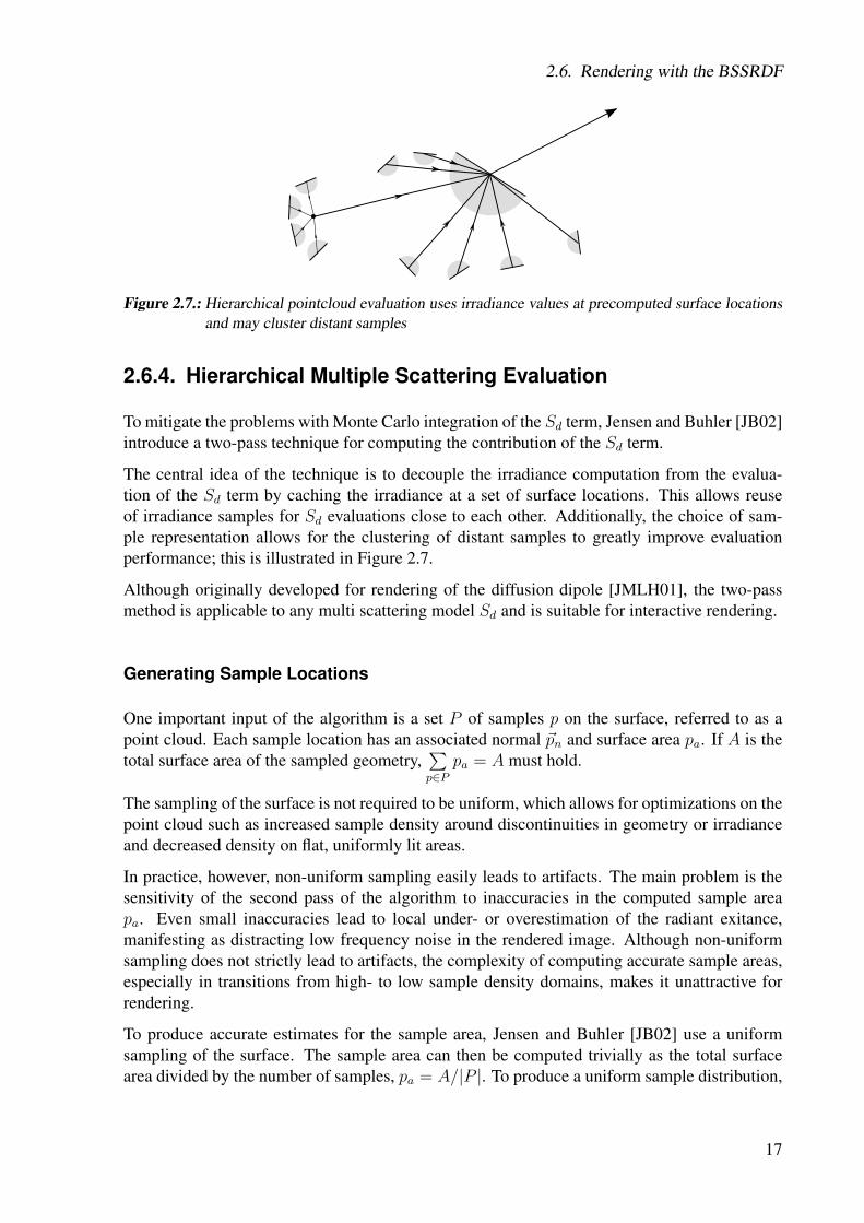
Figure 2.7.: Hierarchical pointcloud evaluation uses irradiance values at precomputed surface locationsand may cluster distant samples

2.6.4. Hierarchical Multiple Scattering Evaluation

To mitigate the problems with Monte Carlo integration of the Sd term, Jensen and Buhler [JB02]introduce a two-pass technique for computing the contribution of the Sd term.

The central idea of the technique is to decouple the irradiance computation from the evalua-tion of the Sd term by caching the irradiance at a set of surface locations. This allows reuseof irradiance samples for Sd evaluations close to each other. Additionally, the choice of sam-ple representation allows for the clustering of distant samples to greatly improve evaluationperformance; this is illustrated in Figure 2.7.

Although originally developed for rendering of the diffusion dipole [JMLH01], the two-passmethod is applicable to any multi scattering model Sd and is suitable for interactive rendering.

Generating Sample Locations

One important input of the algorithm is a set P of samples p on the surface, referred to as apoint cloud. Each sample location has an associated normal ~pn and surface area pa. If A is thetotal surface area of the sampled geometry,

∑p∈P

pa = A must hold.

The sampling of the surface is not required to be uniform, which allows for optimizations on thepoint cloud such as increased sample density around discontinuities in geometry or irradianceand decreased density on flat, uniformly lit areas.

In practice, however, non-uniform sampling easily leads to artifacts. The main problem is thesensitivity of the second pass of the algorithm to inaccuracies in the computed sample areapa. Even small inaccuracies lead to local under- or overestimation of the radiant exitance,manifesting as distracting low frequency noise in the rendered image. Although non-uniformsampling does not strictly lead to artifacts, the complexity of computing accurate sample areas,especially in transitions from high- to low sample density domains, makes it unattractive forrendering.

To produce accurate estimates for the sample area, Jensen and Buhler [JB02] use a uniformsampling of the surface. The sample area can then be computed trivially as the total surfacearea divided by the number of samples, pa = A/|P |. To produce a uniform sample distribution,

17

2. Background

Figure 2.8.: Results for 10 iterations (top), 100 iterations (middle) and 1000 iterations (bottom) of thepoint relaxation algorithm, rendered with the dipole BSSRDF (left, middle) and visualizeddirectly (right). Model courtesy of XYZRGB.

the point repulsion algorithm introduced by Turk [Tur92] is used.

The algorithm works as follows: Starting with an initial guess of uniformly random distributedsamples on the surface, the algorithm performs iterative relaxation of the sample set by comput-ing a repulsion force for each sample point based on the proximity to its neighbours. Each pointis then displaced by the repulsion force. To ensure that each sample still resides on the sur-face after displacement, sample points that are pushed off the polygonal face they reside on areprojected onto their neighbouring polygon if it exists, or clamped to the closest edge otherwise.

The number of relaxation iterations required for a high quality point cloud depends on thecomplexity of the input geometry and the number of sample points. For dense meshes andhigh number of samples, the method may take several hundred or even thousand iterations toconverge to an acceptable result. This is illustrated in Figure 2.8.

Quasi-uniform sampling can be obtained much faster using approximate blue noise methods[KS12], although they introduce low-frequency noise in the rendered image. Since quality ismore important than speed in our case, we use the point repulsion algorithm.

First Pass: Irradiance Sampling

Given the set P of surface samples, the irradiance for each sample has to be computed. Sinceall the samples are placed at the surface of geometry, virtually any standard rendering techniquemay be used.

For offline rendering in a complex setting with occluders, global illumination systems such as

18

2.6. Rendering with the BSSRDF

(a) (b) (c)

Figure 2.9.: Benefits of BSSRDF evaluation with sample clustering compared to evaluation withoutsample clustering, illustrated on a pointcloud with 100′000 samples, rendered at 1680×1050pixels. With sample clustering (a), rendered in 140ms; without sample clustering and equalnumber of samples (b) rendered in 8.5 seconds; no sample clustering and equal render time(140ms) (c) allows only 400 samples. Note that (a) is visually equivalent to (b), despitebeing 60 times faster. Model courtesy of the Stanford Computer Graphics Laboratory.

photon mapping [Jen96] or bi-directional path tracing [LW93] can be employed to compute theirradiance.

For interactive rendering, global illumination techniques are usually too expensive, and methodssuch as shadow mapping [Wil78], which deal only with direct illumination, may be used instead.

Second Pass: BSSRDF Evaluation

Given the set of irradiance samples and an evaluation point ~xo, we now need an efficient methodfor evaluating the radiant exitance at ~xo. Evaluating the sample contributions directly by com-puting the BSSRDF for all irradiance samples is too expensive, since typical point clouds maycontain hundreds of thousands of samples. A better choice is to evaluate the BSSRDF using ahierarchical data structure instead, as illustrated in Figure 2.9. Any hierachical structure can beused that allows efficient traversal and clustering of nearby points.

Jensen and Buhler [JB02] use an octree in their implementation. Each node in the octree con-tains the total surface area Av of all the samples it contains, the total irradiance Ev of all itschildren and an irradiance weighted average location ~Pv. To compute the total radiant exitanceat ~xo, the octree is traversed from the root and each child node is either recursively traversed orevaluated directly, depending on an error heuristic.

Finding an accurate estimation of the error is non-trivial. Jensen and Buhler [JB02] insteadpropose an approximate criterion based on the estimated solid angle ∆ω spanned by a node:

∆ω =Av

|| ~xo − ~Pv||2(2.40)

A node is then recursively traversed if the estimated solid angle is smaller than some user-defined maximum error ε.

19

2. Background

Evaluating the radiant exitance for a leaf node is equivalent to summing the contributions ofthe samples contained in the node. For nodes higher in the hierarchy, the contribution may becomputed by treating the cluster as a single surface point and evaluating the BSSRDF using theaverage location, total irradiance and total area of the node.

It should be noted that the expression in (2.40) is problematic, since the average sample loca-tion is not necessarily an accurate representation of the point distribution. The denominator|| ~xo − ~Px||2 could thus significantly overestimate the distance to the sample set, leading to anerroneously small estimate for the solid angle.

For example, a node with a majority of the samples distant from the evaluation point, but a fewoutliers close to it may not be recursed, since the average location is far from the evaluationpoint. If the node is evaluated directly instead, this may cause significant error, since outliersarbitrarily close to the evaluation point are ignored.

A more conservative estimate is to use the distance to the enclosing bounding box of the nodeinstead. This has the advantage of never overestimating the distance to the sample set, whichavoids errors in the estimated radiant exitance at a higher computational cost.

20

3Implementation

This chapter will describe implementation details of our system. A first section will providea general overview of the system and describe the individual components. The subsequentsections will cover the individual application features in detail.

3.1. System Overview

Our system is built from a set of mostly independent modules, each performing specific tasksdealing with the BSSRDF and tying in with a portion of the user interface. A central controlmodule summarizes parameters and loaded BSSRDFs and ties the rest of the modules together.In the following, the list of the implemented modules is given and described. Details aboutalgorithm implementations are given in sections 3.2 through 3.5. Section 3.6 will cover the userinterface.

Our application has been implemented in C++ and uses the open source, cross-platform UIframework Qt as well as the multi-platform graphics API OpenGL.

3.1.1. Parameter Module

The parameter module summarizes the list of parameters frequently used throughout the appli-cation. These include plot settings, lighting conditions and, most importantly, material parame-ters.

Material parameters consist of the relative index of refraction η, the scattering mean cosine g,the basic unit scale and the absorption and scattering coefficients, σa and σs. The module also

21

3. Implementation

supports an alternative parametrization introduced by Jensen and Buhler [JB02] using the totaldiffuse reflectance Rdr and diffuse mean free path ld instead of σa and σt. Internally, the systemonly works with the physically based parameters σa and σs; parameters entered in the Rdr, ldformat are converted before use. Section 3.4 covers the details of the inversion procedure.

In addition, the parameter module keeps the list of loaded BSSRDFs, both analytic and mea-sured. Analytic BSSRDFs are provided with the material parameters, but may define an ad-ditional set of parameters if so required by the model. These are defined in the BSSRDF fileinterface and are exposed in the user interface. See the appendix A.2 for details about the fileinterface.

3.1.2. Point Cloud Module

The point cloud module provides an implementation of the hierarchical point cloud evaluationdescribed in Section 2.6.4. It allows interactive rendering of a selected loaded BSSRDF (ana-lytic or measured) on an arbitrary triangle mesh (OBJ format) or point cloud (PTC, PDA, PDB,GEO or BGEO format). For triangle meshes, the module generates a point cloud automatically.Generated point clouds are saved to disk in PTC format to speed up future loading times.

The point cloud module supports various different lighting conditions. These include directionallighting, filtered directional lighting and image based lighting (IBL). The filtered directionallighting consists of an ordinary directional light source multiplied with a user specified texture,akin to light falling through stained glass, for example. Its purpose is to allow the user tointroduce discontinuities and different colors into the illumination. The IBL mode computeslighting due to an environment map and optionally supports self-occlusion on the model, whichis more expensive, but much more accurate.

A visual overview of the different lighting modes is given in Figure 3.1.

3.1.3. Lit Sphere Modules

The lit sphere modules consist of two separate modules modelling subsurface scattering on thesphere under a directional light source. The first module computes the subsurface scatteringusing a volumetric path tracer, descibed in Section 3.2. The second module evaluates a selectedanalytic BSSRDF on the sphere using Monte Carlo integration, covered in Section 3.5.

3.1.4. Pencil Beam Module

The pencil beam module computes cross section plots for all loaded BSSRDFs on a half infiniteslab lit by a pencil beam. Plotting modes set in the parameter module control the axes (linear,logarithmic or square root) and color modes (red, green, blue color channels or luminance).Additionally, a reference solution computed by means of a volumetric path tracer, described inSection 3.2, is plotted in the same coordinate system.

22

3.1. System Overview

(a) (b)

(c) (d)

(a) (b)

(c) (d)

Figure 3.1.: Summary of different lighting modes supported by the point cloud module: directional (a),filtered directional (here with checker texture) (b), IBL (c) and occluded IBL (d).Top: Irradiance samples. Bottom: Rendered with dipole BSSRDF. Model courtesy ofXYZRGB. Environment map courtesy of Paul Debevec.

23

3. Implementation

3.2. Volumetric Path Tracing

To support the verification of analytic BSSRDFs, our application provides reference solutionsfor two kinds of geometry: A half-infinite slab lit by a pencil beam, and a sphere under adirectional light source. Both rely on unbiased volumetric path tracing to compute a numericalsolution for the radiance given the material parameters.

Only media with homogeneous scattering properties are considered, greatly simplifying theimplementation and improving the convergence rate. Still, the algorithm remains expensive andcare must be taken to ideally use the available budget of samples.

The path tracing implementation is characterized by a trace function. It traces a random paththrough the medium and returns the exit location as well as the weight of the path. To computethe total radiant exitance at a surface point, the algorithm then only has to repeatedly invoke thetrace function and for each path compute the irradiance at the exit location. The weighted aver-age of the irradiances multiplied by the transmission term then gives the total radiant exitance.

A simple, but naive and inefficient implementation of the trace function is given as follows. Itis a straightforward application of Monte Carlo to the RTE:

1. Start with a position ~x and direction ~ω

2. Pick a random distance s to travel before the next scattering event

3. Advance by s along ~ω and pick a new random direction ~ω′ on the sphere

4. Modify the path weight by extinction e−σts, scattering coefficient σs and phase functionp(~ω · ~ω′)

5. Repeat steps 2-4 until the surface is hit

6. Modify the path weight by the transmission term ft

While simple to implement, this version of the trace function is highly inefficient in that ittakes a large number of samples to converge, especially for materials with high absorption. Theproblem is that path weights rapidly go to zero with the number of scattering events and theamount of distance travelled. The algorithm is completely agnostic of the mean free path, theabsorption coefficient and the scatter anisotropy g.

An improved algorithm distributes samples non-uniformly such that the path weights are con-stant. Intuitively, we still want to sample all paths - to remain unbiased - but would like tomore frequently sample paths that contribute a lot to the final image. By distributing samplingprobabilities corresponding exactly to the path weights, the new path weights are the same forall paths. To achieve this, the naive algorithm has to be modified in four places:

• Don’t pick a uniformly random distance s, but pick it according to the probability densityfunction e−σts

• Instead of choosing the new direction uniformly, choose it with probability according tothe phase function p

• Don’t modify the path weight by the scatter coefficient σs, but perform a Russian roulette,

24

3.2. Volumetric Path Tracing

terminating the path with probability 1− α and continuing with probability α.

• Instead of modifying the weight by the transmission term ft, run a Russian roulette, ex-iting the surface with probability ft and performing internal reflection with probability1− ft.

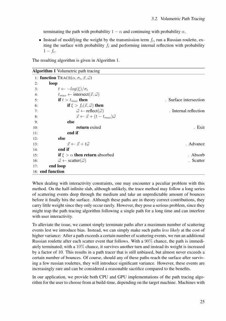
The resulting algorithm is given in Algorithm 1.

Algorithm 1 Volumetric path tracing1: function TRACE(α, σt, ~x, ~ω)2: loop3: t← −log(ξ)/σt4: tmax ← intersect(~x, ~ω)5: if t > tmax then . Surface intersection6: if ξ > ft(~x, ~ω) then7: ~ω ← reflect(~ω) . Internal reflection8: ~x← ~x+ (t− tmax)~ω9: else

10: return exited . Exit11: end if12: else13: ~x← ~x+ t~ω . Advance14: end if15: if ξ > α then return absorbed . Absorb16: ~ω ← scatter(~ω) . Scatter17: end loop18: end function

When dealing with interactivity constraints, one may encounter a peculiar problem with thismethod. On the half-infinite slab, although unlikely, the trace method may follow a long seriesof scattering events deep through the medium and take an unpredictable amount of bouncesbefore it finally hits the surface. Although these paths are in theory correct contributions, theycarry little weight since they only occur rarely. However, they pose a serious problem, since theymight trap the path tracing algorithm following a single path for a long time and can interferewith user interactivity.

To alleviate the issue, we cannot simply terminate paths after a maximum number of scatteringevents lest we introduce bias. Instead, we can simply make such paths less likely at the cost ofhigher variance: After a path exceeds a certain number of scattering events, we run an additionalRussian roulette after each scatter event that follows. With a 90% chance, the path is immedi-ately terminated; with a 10% chance, it survives another turn and instead its weight is increasedby a factor of 10. This results in a path tracer that is still unbiased, but almost never exceeds acertain number of bounces. Of course, should any of these paths reach the surface after surviv-ing a few russian roulettes, they will introduce significant variance. However, these events areincreasingly rare and can be considered a reasonable sacrifice compared to the benefits.

In our application, we provide both CPU and GPU implementations of the path tracing algo-rithm for the user to choose from at build-time, depending on the target machine. Machines with

25

3. Implementation

0 1

2 3

0 0 0 0 0 01 1 1 1 12 2 2 2 23 3 3 0

0 0 1 1 2 20 0 1 2 30 0 1 2 30 1 2 3

Figure 3.2.: Sample set subdivision for octree construction

slower GPUs greatly benefit from the CPU implementation, since long running GPU threadsmay interfere with interactivity of the entire operating system. The CPU implementation on theother hand can run concurrently in background threads, leaving the user interface responsiveeven in the case of long scatter paths.

For the half-infinite slab, our implementation has been verified with the well-tested MCMLbenchmarking tool [WJZ95]. For the lit sphere, the same code is used, with only the primitiveintersection function modified.

3.3. Rendering Translucency

Our system is capable of rendering the BSSRDF on arbitrary meshes and pointclouds undervarious lighting conditions at interactive framerates. To achieve this, we take advantage of thelarge processing powers present in modern programmable GPUs by implementing the two-passpointcloud technique in the OpenGL shading language, GLSL. Timings of our implementationfor various models and point cloud sizes are given in Table 3.1.

26

3.3. Rendering Translucency

Model Size of point cloud Render time

Armadillo 339’679 138msHappy Buddha 301’986 149msBunny 489’088 143msCow 203’355 45msStanford Dragon 88’551 121msLucy 202’801 84msXYZRGB Dragon 199’174 102ms

Table 3.1.: Render times of our GPU pointcloud implementation at a resolution of 1280× 720 pixels ona GTX 480

3.3.1. Point Cloud Generation

If generating a new point cloud is necessary, the algorithm detailed in Section 2.6.4 is em-ployed to generate a sample set uniformly covering the surface. Unfortunately, the algorithmis not easily portable to the GPU, and a CPU implementation is used instead. Since the pointcloud generation represents the most expensive step of the mesh preprocessing pipeline, ourimplementation takes advantage of multiple cores, using OpenMP for parallelization.

Once the point cloud is available, a matching octree is constructed. The octree building algo-rithm starts with the entire sample set, stored in an array. Then, the center location of the sampleset is computed; this partitions the space into eight octants, depending on relative position tothe center. All points in the set are labelled with an index in [0, 7], marking the octant in whichthey are located. The sample array is sorted with a linear time counting sort [Knu98], usingthe octant index as key. This results in 8 or less new sets, formed by all samples with the sameindex. Each of these sets is then recursively subdivided using the same algorithm, until the setsare smaller than some threshold (8 samples in our implementation). The hierarchy of samplesets then forms the octree.

A single subdivision step is illustrated on a 2D example in Figure 3.2.

3.3.2. Irradiance Computation

After generating the point cloud on the CPU, the point samples are transferred to an OpenGLvertex buffer object (VBO). VBOs represent read/writeable regions of GPU memory dedicatedto vertex data and allow the application to store vertices in GPU memory instead of retrans-mitting them at every rendering step. Each vertex stores attributes for position, normal andirradiance.

For the first rendering pass, the application makes use of a vertex shader to compute the irra-diance. Vertex shaders are executed once for each vertex arriving at the vertex transformationstage. In our case, the vertices represent the point samples for which the irradiance is to becomputed.

Normally, the results of the vertex transformation stage are only used for rasterization and then

27

3. Implementation

(a) (b) (c) (d)

Figure 3.3.: Results for different shadow mapping methods: naive (a), with offset (b), with offset andhardware PCF (c) and with offset, hardware PCF and multiple jittered lookups (d). Modelcourtesy of the Stanford Computer Graphics Laboratory.

discarded. However, this behaviour can be modified using transform feedback. Transformfeedback enables the application to stream the results of the vertex transformation stage backinto a VBO. In our case, we disable the rasterization stage completely, compute the sampleirradiance with the vertex shader and stream the results into a second VBO, which is then usedfor rendering.

Some of the implemented lighting techniques perform an incremental computation of the irra-diance. In these cases, the application invokes the vertex shader multiple times and ping-pongsbetween two VBOs used as source and target in turn.

Directional Lighting

Computing irradiance due to a directional light source is trivial except for evaluating the visi-bility of the light source. In our system, we use standard shadow mapping techniques [Wil78]to compute occlusion. In an initial pass, the model is rendered as a depth map from the perspec-tive of the light source into an off-screen buffer. In the irradiance pass, the vertex shader thentransforms each point sample into the coordinate space of the light source and projects it ontothe depth map. If the depth of the point sample in the light coordinate system is larger than thevalue read at at the corresponding cell in the depth map, the sample is assumed to lie in shadow.

A naive implementation of this algorithm easily leads to artifacts due to quantization errorsand limited resolution of the depth buffer, seen in Figure 3.3 (a). Adding a small offset tothe samples read from the depth map removes the majority of artifacts. However, the binaryclassification scheme and the limited resolution of the buffer lead to a blocky appearance ofshadow borders, Figure 3.3 (b). A more visually appealing result can be achieved using per-centage closer filtering (PCF) [RSC87], which averages over multiple shadow lookups. MostGPU hardware provide built-in PCF, performing the depth test on the four closest texels on the

28

3.3. Rendering Translucency

depth buffer and bilinearly interpolating between the four results. Although this improves theappearance of the shadow border, aliasing due to depth map resolution is still clearly visible,Figure 3.3 (c). Performing multiple, jittered lookups, each with hardware PCF, further reducesaliasing artifacts and helps smooth out the shadow border, Figure 3.3 (d).

Image Based Lighting

Computing the irradiance due to an environment map is a lot more costly than for the purelydirectional case, since we now have to compute the integral of the incident radiance over thehemisphere of incident directions. Implicitly, this was already the case for the directional light,but because the incident light was represented by a delta function, the integral collapses andresults in a very simple expression. For the environment map, now all incident directions canpotentially carry radiance, requiring full evaluation of the integral.

We can build an approximation of the true irradiance by noting that if occlusion is ignored,the irradiance no longer depends on the location of the sample point, but only on the surfacenormal. This allows precomputation of the integral for a set of possible surface normals, suchthat at runtime, only a lookup of the precomputed integral has to be performed. This allows forfast estimation of the irradiance even when the model or the environment map are rotated. Inour system, precomputation of the integral is performed when an environment map is loaded bythe user. The integral is approximated by a Monte Carlo method, computed for a large set ofpossible surface normals and then stored in a cubemap. At runtime, the vertex shader only hasto perform a lookup in the cubemap texture using the surface normal.

Although this method is fast, disregarding self-occlusion by the mesh results in overestimationof the irradiance at most locations, seen in Figure 3.1 (c). These artifacts can only be removedby evaluating the integral while taking occlusion into account. Not only does this require aper-point sample evaluation of the integral each time the lighting is changed, thwarting precom-putation - it also necessitates a method to compute the visibility of a point on the environmentmap seen from a surface point. In offline rendering, typically geometric ray-surface intersec-tions are used to compute visibility, which makes the process unfeasibly slow for interactiverendering, especially for large point clouds and complex meshes.

However, we can speed up this process by taking advantage of shadow mapping techniques.The integral is still computed with a Monte Carlo method as before, but instead of choosingsamples individually for each surface point, we choose the same samples for all points instead.This way, we can pick a sample on the environment map and treat it as a directional light source,allowing the use of a shadow map to compute visibility for each surface point. Although a fullshadow map has to be computed for each sample, it contributes to all points at the same time,greatly improving performance [PH10]. It should be noted that choosing the same samples forall surface points leads to banding artifacts if few samples are used.

3.3.3. Radiance Evaluation

For the second rendering pass, a representation of the octree in GPU memory is required. SinceGLSL does not support full access to GPU memory, the data structure has to be stored in

29

3. Implementation

A

B C D

Point sample texture

Child descriptor texture

A B C D

Figure 3.4.: Layout of the descriptor arrays. Top: Example octree. Middle: Child descriptor array.Bottom: Point sample array. Not shown: Node attribute arrays

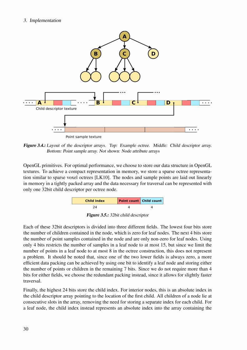
OpenGL primitives. For optimal performance, we choose to store our data structure in OpenGLtextures. To achieve a compact representation in memory, we store a sparse octree representa-tion similar to sparse voxel octrees [LK10]. The nodes and sample points are laid out linearlyin memory in a tightly packed array and the data necessary for traversal can be represented withonly one 32bit child descriptor per octree node.

Child index Point count Child count

24 4 4

Figure 3.5.: 32bit child descriptor

Each of these 32bit descriptors is divided into three different fields. The lowest four bits storethe number of children contained in the node, which is zero for leaf nodes. The next 4 bits storethe number of point samples contained in the node and are only non-zero for leaf nodes. Usingonly 4 bits restricts the number of samples in a leaf node to at most 15, but since we limit thenumber of points in a leaf node to at most 8 in the octree construction, this does not representa problem. It should be noted that, since one of the two lower fields is always zero, a moreefficient data packing can be achieved by using one bit to identify a leaf node and storing eitherthe number of points or children in the remaining 7 bits. Since we do not require more than 4bits for either fields, we choose the redundant packing instead, since it allows for slightly fastertraversal.

Finally, the highest 24 bits store the child index. For interior nodes, this is an absolute index inthe child descriptor array pointing to the location of the first child. All children of a node lie atconsecutive slots in the array, removing the need for storing a separate index for each child. Fora leaf node, the child index instead represents an absolute index into the array containing the

30

3.4. Parameter Inversion

point samples; again, all points of a leaf node are laid out consecutively in memory, requiringonly the array index to address all points of a leaf node. The layout of the descriptors in memoryis illustrated in Figure 3.4.

The internal nodes also carry information about the total irradiance, the total area, the irradianceweighted average location and the bounding box of the point samples represented by the node.The irradiance (RGB) and total area (1 float) are merged and stored in a single, 4 channel floattexture. Lower- and upper bound of the bounding box as well as the average location are allvectors of 3 floats, but unfortunately, 3 channel textures are not widely supported in OpenGL.Subsequently, these attributes, too, are stored in 4-channel float textures, leaving one colorchannel per attribute unused. Although 1D textures most closely mirror the nature of arrays,most OpenGL implementations limit the size of 1D textures to a size much smaller than requiredfor most octrees. Instead, we store the arrays in 2D textures using row-major order.

Traversal of the octree to compute the radiant exitance closely follows Jensen and Buhler[JB02]. Starting with the root node, the shader recursively traverses its child nodes as longas the error according to the solid angle criterion is too big and evaluates the BSSRDF other-wise. One problem with this formulation is that GPUs do not have a stack, making “recursivetraversal” in the traditional sense impossible. For this reason, the shader uses a loop insteadof recursion and keeps track of previous iterations manually using an array. It should be notedthat arrays in GLSL internally incur a high cost in terms of shader complexity. The array sizealso stands in direct relation to usage of limited GPU resources by the shader, thus limiting theamount of threads that can be executed concurrently.

For this reason, reducing the size of the stack (and therefore the array) to a minimum is impor-tant for shader performance. We note that for traversal, each level of the stack needs to storethe array index of the node currently being processed and the number of child nodes left tovisit. By storing the array index in the upper 24 bits and the child count in the lower 8 bits ofan integer, we can reduce the storage requirement for each recursion to a single 32bit integer.In the application, we limit the maximum depth of the octree to 10 levels (allowing for up to8.5× 109 sample points), and can thus safely compact the stack to an array of 10 32bit integers.

Pseudocode of our traversal routine is found in Algorithm 2.

3.4. Parameter Inversion

Following Jensen et al. [JMLH01], we support an alternative parametrization of the BSSRDFusing the total diffuse reflectance Rdr and diffuse mean free path ld in place of absorption andscattering coefficient σa and σs. This is motivated by the fact that the effects of σa and σs on therendered image are highly non-linear, making it difficult to predict the appearance of a modelwith subsurface scattering for a given set of parameters.

The alternative parametrization makes it easier to control the rendered image. Intuitively, thetotal diffuse reflectanceRdr controls the color of surfaces under direct light, whereas the diffusemean free path ld controls the color of the scattered light on surfaces that lie in shadow. Addi-tionally, the magnitude of ld controls the translucency of the material. Large values for ld resultin more translucent materials, and vice-versa.

31

3. Implementation

Algorithm 2 Octree traversal1: radiance← 02: node← 03: childnum← 04: loop5: if subdivide(node) then6: recurse(node, childnum)7: else8: if is leaf(node) then9: radiance← radiance + point contributions(node)

10: else11: radiance← radiance + node contribution(node)12: end if13: next node(node, childnum)14: end if15: end loop16:17: function RECURSE(node, childnum)18: if node 6= 0 then push(node, childnum)19: node← last child(node)20: childnum← child count(node) − 121: end function22:23: function NEXT NODE(node, childnum)24: if childnum = 0 then25: unrecurse()26: else27: node← node− 128: childnum← childnum− 129: end if30: end function31:32: function UNRECURSE

33: if stack empty then34: set result(radiance)35: end shader()36: else37: node, childnum← pop()38: end if39: end function

32

3.5. BSSRDF Integration on the Sphere

To render an image with the alternative parametrization, the parameters have to be invertedto give the corresponding values of σa and σs. The total diffuse reflectance is defined as theintegral of the diffuse reflectance profile:

Rdr = 2π

∫ ∞0

Rd(r)rdr (3.1)

For the diffusion dipole, this yields [JB02]:

Rd =α′

2

(1 + e−

43A√

3(1−α′))e−√

3(1−α′) (3.2)

In general, we can formulate Rdr as a function of the reduced albedo α′ and the internal reflec-tion parameter A. Solving this function for α′ yields a term depending on A and Rdr, which aregiven. Then, the rest of the parameters can be computed using α′ and ld:

σ′t =1

ld√

3(1− α′)(3.3)

σ′s = α′σ′t (3.4)σa = σ′t − σ′s (3.5)

In our implementation, we cannot analytically solve for α′, since we allow any BSSRDF tobe defined and therefore can’t assume any knowledge about Rd or Rdr. Instead, we definea function stub to evaluate Rdr given α′ in our file interface, which can be implemented bythe BSSRDF. A standard bisection root solver is then employed to solve for α′ numerically.Although more sophisticated numerical root solvers can show superior convergence to the bi-section method, we found them to become unstable for some Rdr functions. Additionally, thebisection method is easily parallelizable, allowing us to take advantage of the GPU.

In our implementation, we start with the interval [0, 1] and divide it into 512 equally spacedsubintervals. We then run a shader computing the value of Rdr for the end points of each ofthe subintervals in parallel. Then, the subinterval containing the user-specified Rdr is selectedand the process is repeated. The selected subinterval gives the bounds for α′. We repeat thisprocedure three times, guaranteeing a maximum error of 2−27 for α′, which is beyond floatingpoint accuracy for the majority of input values.

3.5. BSSRDF Integration on the Sphere

Complementary to the hierarchical pointcloud renderer, we also provide a module renderingthe BSSRDF on a sphere with Monte Carlo integration. Motivation for this module is to allowcomparison with a volumetric path tracer with the same geometry and lighting conditions. Thepoint cloud, although fast, introduces discretization error; Monte Carlo integration howeverconverges to the correct value of the double integral (2.14).

33

3. Implementation

Performing the Monte Carlo integration is straightforward. First, a uniformly random positionon the sphere is picked. Then the BSSRDF is evaluated. The sum of the contributions dividedby the individual sample probabilities yields an estimate for the radiant exitance.

Note that this formulation is inefficient if the integrand is strongly peaked and may take manysamples to converge. Ideally, the method would apply importance sampling to pick sampleson the sphere. Unfortunately, we cannot make any assumptions about the integrand, sincewe allow the user to define any function for the BSSRDF. Providing an importance samplinginterface general enough to handle all BSSRDFs exceeds the scope of this thesis and is left forfuture work.

34

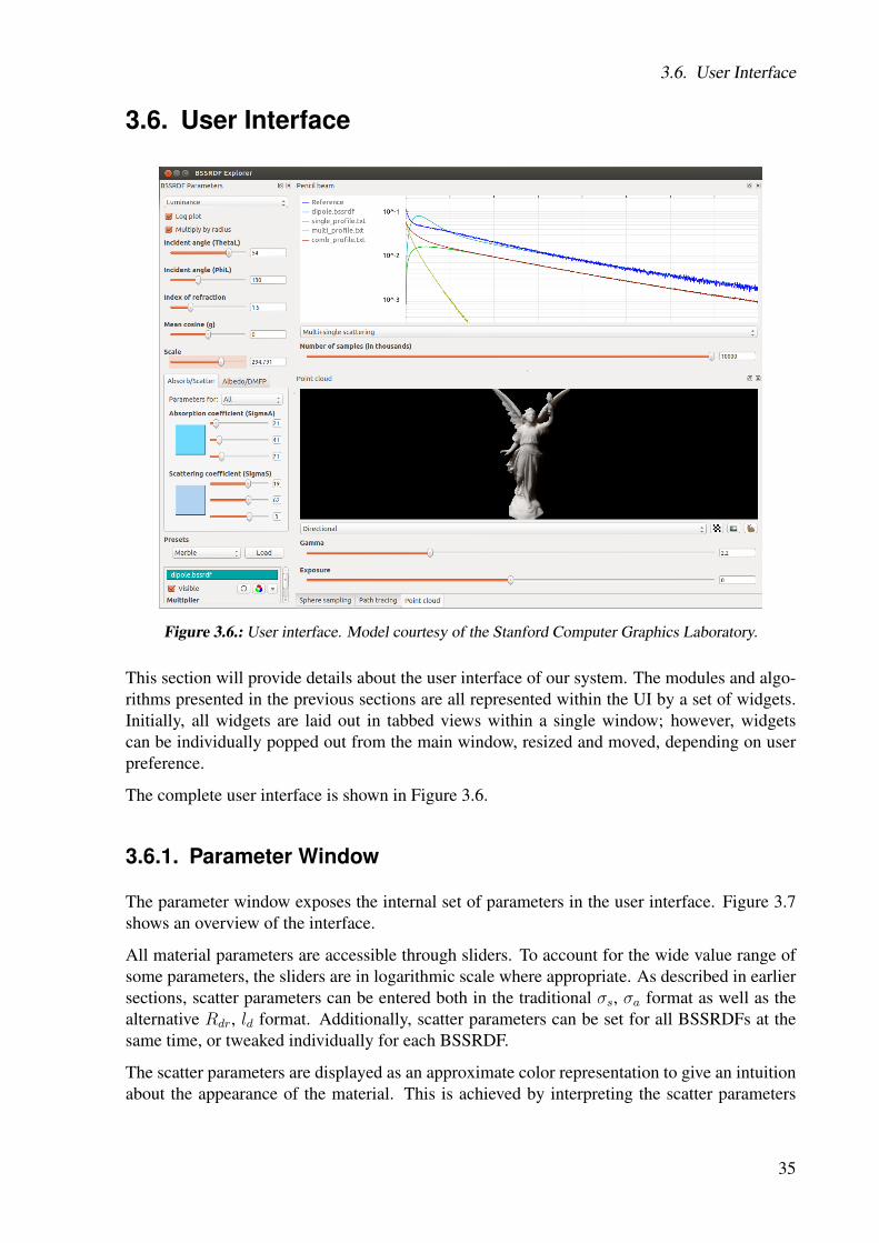
3.6. User Interface

3.6. User Interface

Figure 3.6.: User interface. Model courtesy of the Stanford Computer Graphics Laboratory.

This section will provide details about the user interface of our system. The modules and algo-rithms presented in the previous sections are all represented within the UI by a set of widgets.Initially, all widgets are laid out in tabbed views within a single window; however, widgetscan be individually popped out from the main window, resized and moved, depending on userpreference.

The complete user interface is shown in Figure 3.6.

3.6.1. Parameter Window

The parameter window exposes the internal set of parameters in the user interface. Figure 3.7shows an overview of the interface.

All material parameters are accessible through sliders. To account for the wide value range ofsome parameters, the sliders are in logarithmic scale where appropriate. As described in earliersections, scatter parameters can be entered both in the traditional σs, σa format as well as thealternative Rdr, ld format. Additionally, scatter parameters can be set for all BSSRDFs at thesame time, or tweaked individually for each BSSRDF.

The scatter parameters are displayed as an approximate color representation to give an intuitionabout the appearance of the material. This is achieved by interpreting the scatter parameters

35

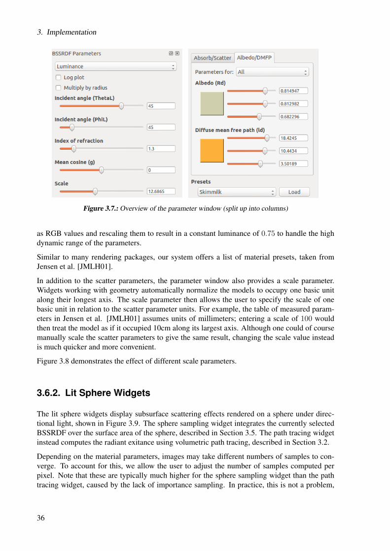
3. Implementation

Figure 3.7.: Overview of the parameter window (split up into columns)

as RGB values and rescaling them to result in a constant luminance of 0.75 to handle the highdynamic range of the parameters.

Similar to many rendering packages, our system offers a list of material presets, taken fromJensen et al. [JMLH01].

In addition to the scatter parameters, the parameter window also provides a scale parameter.Widgets working with geometry automatically normalize the models to occupy one basic unitalong their longest axis. The scale parameter then allows the user to specify the scale of onebasic unit in relation to the scatter parameter units. For example, the table of measured param-eters in Jensen et al. [JMLH01] assumes units of millimeters; entering a scale of 100 wouldthen treat the model as if it occupied 10cm along its largest axis. Although one could of coursemanually scale the scatter parameters to give the same result, changing the scale value insteadis much quicker and more convenient.

Figure 3.8 demonstrates the effect of different scale parameters.

3.6.2. Lit Sphere Widgets

The lit sphere widgets display subsurface scattering effects rendered on a sphere under direc-tional light, shown in Figure 3.9. The sphere sampling widget integrates the currently selectedBSSRDF over the surface area of the sphere, described in Section 3.5. The path tracing widgetinstead computes the radiant exitance using volumetric path tracing, described in Section 3.2.

Depending on the material parameters, images may take different numbers of samples to con-verge. To account for this, we allow the user to adjust the number of samples computed perpixel. Note that these are typically much higher for the sphere sampling widget than the pathtracing widget, caused by the lack of importance sampling. In practice, this is not a problem,

36

3.6. User Interface

(a) (b) (c) (d)

Figure 3.8.: Influence of the scale parameter on the rendered image: Values of 10 (a), 50 (b), 200 (c) and500 (d) for the dipole BSSRDF, from the front (top) and back (bottom). Model courtesy ofthe Stanford Computer Graphics Laboratory.

since computing a BSSRDF sample is many magnitudes cheaper in terms of computation timecompared to tracing a full scatter path through the medium.

Initially, the widgets are grouped into a tabbed view. This allows quickly switching betweenthe two rendered images, making it easier to spot differences in the results. Like all widgets,they may also be popped out from the main window and rescaled to allow for a side by sidecomparison, such as shown in Figure 3.9.

Both widgets perform rendering in high dynamic range (HDR) and support post-process gammacorrection and exposure adjustment using sliders, as seen in Figure 3.9.

3.6.3. Pencil Plot Widget

The pencil plot widget shows cross section plots of all loaded BSSRDFs, evaluated on a semi-infinite slab illuminated by a pencil beam in the origin. Additionally, a reference solution isplotted, computed with volumetric path tracing.

37

3. Implementation

Figure 3.9.: Overview of the lit sphere widgets

Comparing BSSRDFs in a linear plot can be problematic, since they typically cover large valueranges. The plot thus supports both linear and logarithmic scales on the y axis. Logarithmicplots are common in fields other than image synthesis, because they allow accurate comparisonfor regions far away from the source where the function values are small. For image synthesishowever, regions close to the source, where the function values are large, are more important,since they influence the light transport the most. Logarithmic plots can be problematic here,because they might downplay large errors near the source - for example, the values 10 and 20appear to have the same distance in the log plot as 0.01 and 0.02.

For this reason, the widget also supports a square root scale on the y axis as a useful addition tologarithmic plots, allowing a more accurate visual comparison near the source. Complementaryto different axis scales, the widget also supports plotting the product of radius from the originand BSSRDF, which is a useful modification to damp the strong peak near the source. Allplotting features may be enabled or disabled individually from the parameter window.

It should be noted that all BSSRDFs compute results in RGB, whereas the plot only displaysa single value per BSSRDF. To account for this, the plot may be adjusted to either display theluminance or the red, green or blue color channel. In addition, a single BSSRDF can be selectedto be “soloed”, hiding all other BSSRDFs and displaying the color channels of the BSSRDF asseparate graphs in the plot.

Similar to the path trace widget, the number of samples computed for the path traced solutionmay be adjusted to account for different materials.

38

3.6. User Interface

Figure 3.10.: Overview of the pencil plot widget

3.6.4. Point Cloud Widget

The point cloud widget is the most useful widget to evaluate the visual performance of a BSS-RDF. It allows rendering any BSSRDF on arbitrary triangular meshes or point clouds and sup-ports various lighting modes.

When loading a model, the widget makes an attempt at finding both a polygonal as well as apoint cloud representation of the model on the file system. If both are available, the polygonalmesh is used for rendering and the point cloud to sample the irradiance. If only a polygonalmesh is available, a point cloud representation is generated and the result is cached to disk.Vice-versa, if only the point cloud is available, an approximate polygonal reconstruction isgenerated and used for rendering. Internally, the system uses the Partio library [Stu10] forefficient point cloud input/output, supporting most popular point cloud formats.

A visual summary of the supported lighting modes is given in Figure 3.1. The occluded IBLmode is comparatively expensive and would take too much time if computed directly. Instead,the irradiance is constructed incrementally, computing only a few samples every frame, allow-ing for visual feedback on the construction as well as intermediate user input. We can also takeadvantage of the fact that camera rotation does not influence the illumination, making recom-puting the irradiance unnecessary when only the camera is changed.

Although the rendering step generally performs well, the framerate may drop too low for com-plex models and large resolutions. For this reason, the image is only rendered at half the regularresolution when the environment is changing, for example due to material or camera changes.Once the environment is at rest, the full resolution image is computed.

Similar to the lit sphere widgets, the point cloud widget renders in high dynamic range andsupports post-process gamma correction and exposure adjustment.

39

4Conclusion and Future Work

In this thesis, we presented an extensible rendering and analysis framework for the BSSRDF.We summarized existing research in the field and implemented the presented rendering tech-niques on graphics hardware, allowing for rendering at interactive framerates. We implementedunbiased rendering methods, both on CPU and GPU, to provide reference solutions for sim-ple geometries. We implemented the classic diffusion dipole [JMLH01] and the better dipole[d’E12] in our system. We implemented plotting tools to study the cross-section behaviour ofBSSRDFs. We implemented our work in a multi-platform GUI application, building on thepopular BRDF Explorer by Walt Disney Animation Studios. We hope that our system becomesuseful to researchers and artists alike and, by releasing the application as an open source project,hope that the system can be improved even after this thesis.

Future improvements include extending the BSSRDF interface with an importance samplingframework to properly handle strongly peaked BSSRDFs. It would also be useful to add avolumetric path tracer for arbitrary geometry to compare the appearance of the BSSRDF onarbitrary meshes to a reference solution. Another interesting feature to consider is integrationof surface BRDFs into the application to increase the visual fidelity of the rendered images.

41

AAppendix

A.1. Efficient Pseudorandom Float Generation

One of the core ingredients of a fast and accurate path tracer is a good pseudorandom numbergenerator (PRNG). A PRNG is only pseudorandom, because its output sequence is determin-istic, periodic and reproducible given the same seed value. Truly random number sequencesare hard to produce on a deterministic machine, but “good enough” pseudorandomness sufficesfor most purposes. A PRNG suitable for Monte Carlo integration has to fulfill the followingproperties:

• Guaranteed long sequence periods

• Uniform distribution of the generated numbers within the PRNG value range

• No correlation between successive values

Several PRNGs fulfill these properties and are fast enough for Monte Carlo integration, suchas linear congruental generators (LCG) [Knu81], lagged fibonacci generators (LFG) [Bre92] orthe Mersenne Twister [MN98].

LCGs are attractive for GPUs, because they require minimal storage and are fast to compute.An LCG is defined by the recurrence relation

Xn+1 ≡ (aXn + c) (mod N) (A.1)

Where N is the value range, Xn is the current state, X0 is the start value (“seed”) and a and care the parameters of the LCG. Care must be taken when choosing a and c, since bad choicesmay lead to disastrously short periods, greatly distorting results gained through Monte Carlo

43

A. Appendix

methods. For our implementation, we use m = 231, a = 1103515245, c = 12345, correspond-ing to ANSI C rand[Ent97]. This generator has a full period length of 231, although it has beennoted that “the low bits of the numbers generated are not very random” [Ent97]. This is fine forour purposes, since we only use the upper 23 bits (see below).

Typically, path tracing implementations require uniform floating point numbers in [0, 1) or[−1, 1) range and not integers that most PRNGs produce. A straightforward way to construct afloating point PRNG is to simply use an integer PRNG and divide the returned number sequenceby N . While this method achieves the desired result, it is comparably expensive, requiring bothan integer-to-floating point conversion as well as a floating point division. For a volumetric pathtracer, large amounts of random floats are consumed for little computation, easily making thePRNG the bottleneck of the algorithm.

Thus, a fast conversion between integer PRNGs and floating points in the desired value rangeis of high interest for fast Monte Carlo integrators. In our implementation, we exploit the IEEE754 float representation [otICS08] and GPU intrinsics.

Sign Exponent Mantissa

81 23

Figure A.1.: IEEE Float representation

The layout of the IEEE float is given in Figure A.1. A float is represented as a 32 bit string,partitioned into three fields. Here, we denote s as the sign bit, m as the mantissa and q asthe biased exponent. Then we can define the significand c = 1.m and the unbiased exponente = q − 127. This yields the normalized float representation

(−1)s × c× 2e (A.2)

It should be noted that, for increased precision, the IEEE float format always adds an impliedleading 1 in front of the mantissa m, leading to the perhaps odd notation of 1.m

We can now use this representation to our advantage to efficiently generate a random floatingpoint number in [0, 1) using a two-step construction. First, a random float in [1, 2) is produced.By setting the bits corresponding to the mantissa to a random 23 bit integer k and letting s = 0,q = 127, (A.2) yields

(−1)0 × 1.k × 2127−127 = 1.k (A.3)

Which is a floating point number in range [1, 2). Simply subtracting 1 from this number yieldsthe desired random floating point in [0, 1).

Similarly, we can generate a random floating point in range [−1, 1) following the previousconstruction, but setting q = 128 instead. This gives us

(−1)0 × 1.k × 2128−127 = 2× 1.k (A.4)

44

A.2. BSSRDF Interface

Which is a floating point number in range [2, 4). Simply subtracting 3 gives us the desired[−1, 1) distribution.

Contructing the corresponding floating point bit representation from the result of a PRNG iseasily achieved using bit level operators present in most programming languages. Typically,these operators are only available for integers and not for floats, making a direct construc-tion of the desired floating point number difficult. Fortunately, GLSL offers an instructionuintBitsToFloat, which takes an unsigned 32 bit integer and reinterprets it as a floatingpoint number without conversion.

Using this instruction, we can first construct the floating point bit representation using bit leveloperators on integers. The result is then reinterpreted as a floating point number and the floatingpoint subtraction is performed.

GLSL code for generating pseudorandom floating point numbers as described in this sectioncan be found in Listing A.1. Note that on current hardware, uintBitsToFloatperforms noactual operation and only serves as an instruction to the compiler, making the conversion freein terms of computation.

Listing A.1: GLSL pseudorandom float generation/∗ Has t o be i n i t i a l i z e d t o seed v a l u e b e f o r e use ∗ /u i n t RandSeed ;

/∗ R e t u r n s f l o a t i n r a n g e [ 0 , 1 ) . P e r i o d l e n g t h i s 2^31 ∗ /f l o a t Rand ( )

RandSeed = (1103515245 u∗RandSeed + 12345 u ) & 0x7FFFFFFFu ;

u i n t F l o a t B i t s = ( RandSeed >> 8u ) | 0 x3F800000u ;

re turn u i n t B i t s T o F l o a t ( F l o a t B i t s ) − 1 . 0 ;

/∗ R e t u r n s f l o a t i n r a n g e [−1 , 1 ) . P e r i o d l e n g t h i s 2^31 ∗ /f l o a t Rand2 ( )

RandSeed = (1103515245 u∗RandSeed + 12345 u ) & 0x7FFFFFFFu ;

u i n t F l o a t B i t s = ( RandSeed >> 8u ) | 0 x40000000u ;

re turn u i n t B i t s T o F l o a t ( F l o a t B i t s ) − 3 . 0 ;

A.2. BSSRDF Interface

Instead of implementing analytic BSSRDFs inside the application code, our system makes useof an extensible system based on human-readable text files. These files carry the extension*.bssrdf and describe attributes of the BSSRDF, expose parameters to the user interface anddefine analytic functions later invoked by the application.

The first line of a BSSRDF file must contain a list of attributes describing the BSSRDF. The restof the file consists of a list of sections in arbitrary order. These sections contain either parameter

45

A. Appendix

declarations parsed by the application or segments of GLSL code, which are pieced togetherwith code from our system to produce various shaders responsible for rendering. Sections areenclosed within a ::begin . . . ::end block and must be named. If the name of a section isnot recognized by the application, it is ignored.

The following paragraphs describe the attributes and sections in detail. An example BSSRDFfile for the diffusion dipole is given in listing A.2.

Attributes The list of attributes currently recognized by the application are as follows:

1. analytic: This BSSRDF is in analytic form. This attribute is mandatory for all BSSRDFfiles.

2. radial: The BSSRDF only depends on ||xo − xi||, not the relative position of xi and xo

3. no_wi: BSSRDF does not depend on incident direction

4. no_wo: BSSRDF does not depend on exitant direction

The radial attribute provides an important hint to the point cloud module, in that the BSSRDFcan be represented by a radial profile. This allows the module to precompute the profile into a1D texture and only perform texture lookups when rendering, greatly improving performance.

Parameters Section A BSSRDF may define a list of parameters exposed in the user inter-face. The application allows float, boolean and colour parameters. Parameter declarations areof the form

float [name] [minimum value] [maximum value] [default value]bool [name] [default value]color [name] [default red] [default green] [default blue]

Parameters defined this way are available as uniforms to the shader and can be referred to likeany other variable in the GLSL code.

Initializer Section The intializer section allows the BSSRDF to define an init()function,which is invoked once before the first evaluation of the BSSRDF. It is useful to precomputevalues frequently used in the evaluation of the BSSRDF to improve performance.

Diffuse Reflection Section To support inversion of parameters from the Rdr, ld format toσa, σs format, a BSSRDF must provide a DiffuseReflectance function, which computesthe value ofRdr given α′. This section can be omitted, in which case theRdr, ld parametrizationis disabled for this BSSRDF.

Shader Section The shader section contains the rest of the GLSL code and defines theanalytic BSSRDF function, which computes the value of the BSSRDF given incident posi-tion/direction and exitant position/direction.

46

A.2. BSSRDF Interface

Listing A.2: Diffusion dipole *.bssrdfa n a l y t i c r a d i a l no_wi no_wo

: : b e g i n p a r a m e t e r sf l o a t M u l t i p l i e r 0 . 0 1 0 . 0 1 . 0: : end p a r a m e t e r s

: : b e g i n i n i t i a l i z e r

vec3 Lu ;vec3 AlphaPr ime ;vec3 SigmaTr ;f l o a t A;

void i n i t ( ) f l o a t Fdr = −1 .44 / ( IOR∗IOR ) + 0 . 7 1 / IOR + 0 .668 + 0 .0636∗ IOR ;A = ( 1 . 0 + Fdr ) / ( 1 . 0 − Fdr ) ;

vec3 SigmaSPrime = SigmaS ∗ ( 1 . 0 − G ) ;vec3 SigmaTPrime = SigmaSPrime + SigmaA ;SigmaTr = s q r t ( 3 . 0 ∗ SigmaA∗SigmaTPrime ) ;AlphaPr ime = SigmaSPrime / SigmaTPrime ;Lu = 1 . 0 / SigmaTPrime ;

: : end i n i t i a l i z e r

: : b e g i n d i f f u s e R e f l e c t a n c e

vec3 D i f f u s e R e f l e c t a n c e ( vec3 AlphaPr ime ) vec3 T = s q r t ( 3 . 0 ∗ ( 1 . 0 − AlphaPr ime ) ) ;re turn AlphaPr ime ∗ 0 . 5 ∗ ( 1 . 0 + exp ( −4 . 0 / 3 . 0∗A∗T ) ) ∗ exp(−T ) ;

: : end d i f f u s e R e f l e c t a n c e

: : b e g i n s h a d e r

vec3 B s s r d f ( vec3 Xi , vec3 Wi , vec3 Xo , vec3 Wo) vec3 R = vec3 ( d o t ( Xi − Xo , Xi − Xo ) ) ;vec3 Zr = Lu ;vec3 Zv = Lu ∗ ( 1 . 0 + 4 . 0 / 3 . 0 ∗A ) ;vec3 Dr = s q r t (R + Zr∗Zr ) ;vec3 Dv = s q r t (R + Zv∗Zv ) ;vec3 C1 = Zr ∗ ( SigmaTr + 1 . 0 / Dr ) ;vec3 C2 = Zv ∗ ( SigmaTr + 1 . 0 / Dv ) ;vec3 FluenceR = C1∗ exp(−SigmaTr∗Dr ) / ( Dr∗Dr ) ;vec3 FluenceV = C2∗ exp(−SigmaTr∗Dv ) / ( Dv∗Dv ) ;

re turn M u l t i p l i e r / ( 4 . 0 ∗ PI )∗ AlphaPr ime ∗ ( FluenceR + FluenceV ) ;

: : end s h a d e r

47

Bibliography

[Bre92] Richard P. Brent. Uniform random number generators for supercomputers. InProc. Fifth Australian Supercomputer Conference, pages 95–104, 1992.

[Bry91] G. H. Bryan. An application of the method of images to the conduction of heat. InProceedings of the London Mathematical Society, pages 424–430, 1891.

[Cha58] Subrahmanyan Chandrasekhar. Proceedings of the National Academy of Sciencesof the United States of America, chapter 9, pages 933–940. Number v. 44. NationalAcademy of Sciences, 1958.

[d’E12] Eugene d’Eon. A better dipole, 2012.

[DI11] Eugene D’Eon and Geoffrey Irving. A quantized-diffusion model for renderingtranslucent materials. ACM Trans. Graph., 30(4):56:1–56:14, July 2011.

[DJ05] Craig Donner and Henrik Wann Jensen. Light diffusion in multi-layered translu-cent materials. ACM Trans. Graph., 24(3):1032–1039, July 2005.

[dL07] Eugene d’Eon and David Luebke. Advanced techniques for realistic real-time skinrendering. GPU Gems, 3, 2007.

[EH79] W.G. Egan and T.W. Hilgeman. Optical properties of inhomogeneous materials:applications to geology, astronomy, chemistry, and engineering. Academic Press,1979.

[Ent97] Karl Entacher. A collection of selected pseudorandom number generators withlinear structures, 1997.

[FPBP09] Adrià Forés, Sumanta N. Pattanaik, Carles Bosch, and Xavier Pueyo. BRDFLab:A general system for designing BRDFs. In Proceedings CEIG’09. Eurographics,

Bibliography

2009.

[FPW92] T. J. Farrell, M. S. Patterson, and B. Wilson. A diffusion theory model of spa-tially resolved, steady-state diffuse reflectance for the noninvasive determinationof tissue optical properties in vivo. Medical Physics, 19(4):879–888, July 1992.

[HK93] P. Hanrahan and W. Krueger. Reflection from layered surfaces due to subsurfacescattering. In Computer Graphics, SIGGRAPH 93 Proceedings, pages 165–174,Anaheim, CA, aug 1993.

[Jar08] Wojciech Jarosz. Efficient Monte Carlo Methods for Light Transport in ScatteringMedia. PhD thesis, UC San Diego, September 2008.

[JB02] H. W. Jensen and J. Buhler. A rapid hierarchical rendering technique for translucentmaterials. In Computer Graphics, SIGGRAPH 2002 Proceedings, pages 576–581,Los Angeles, CA, jul 2002.

[Jen96] Henrik Wann Jensen. Global illumination using photon maps. Rendering Tech-niques ’96, pages 21–30, 1996.

[Jen01] H. W. Jensen. Realistic Image Synthesis Using Photon Mapping. AK Peters, 2001.ISBN: 1568811470.

[JG10] Jorge Jimenez and Diego Gutierrez. GPU Pro: Advanced Rendering Techniques,chapter Screen-Space Subsurface Scattering, pages 335–351. AK Peters Ltd.,2010.

[JMLH01] H. W. Jensen, S. R. Marschner, M. Levoy, and P. Hanrahan. A practical model forsubsurface light transport. In Computer Graphics, SIGGRAPH 2001 Proceedings,pages 511–518, Los Angeles, CA, aug 2001.

[JWSG10] Jorge Jimenez, David Whelan, Veronica Sundstedt, and Diego Gutierrez. Real-timerealistic skin translucency. IEEE Computer Graphics and Applications, 30(4):32–41, 2010.

[Kaj86] James T. Kajiya. The rendering equation. In SIGGRAPH, pages 143–150, 1986.

[Knu81] Donald E. Knuth. The Art of Computer Programming, Volume II: SeminumericalAlgorithms, 2nd Edition. Addison-Wesley, 1981.

[Knu98] Donald E. Knuth. The art of computer programming, volume 3: (2nd ed.) sortingand searching. Addison Wesley Longman Publishing Co., Inc., Redwood City,CA, USA, 1998.

[Kor69] G. Kortüm. Reflectance spectroscopy: Principles, methods, applications. Springer,1969.

[KS12] Nima Khademi Kalantari and Pradeep Sen. Fast generation of approximate bluenoise point sets. Computer Graphics Forum, 31(4):1529–1535, 2012.

[LK10] Samuli Laine and Tero Karras. Efficient sparse voxel octrees. In Proceedings ofACM SIGGRAPH 2010 Symposium on Interactive 3D Graphics and Games, pages55–63. ACM Press, 2010.

50

Bibliography

[LW93] Eric P. Lafortune and Yves Willems. Bi-directional path tracing. In Compugraph-ics ’93,, pages 145–153, Dec 1993.

[MN98] Makoto Matsumoto and Takuji Nishimura. Mersenne twister: a 623-dimensionallyequidistributed uniform pseudo-random number generator. ACM Trans. Model.Comput. Simul., 8(1):3–30, January 1998.

[MoEP90] J.D. Moulton and McMaster University. Dept. of Engineering Physics. DiffusionModelling of Picosecond Laser Pulse Propagation in Turbid Media. McMasterUniversity, 1990.

[NRH+77] F. Nicodemus, J. Richmond, J. Hsia, I. Ginsberg, and T. Limperis. Geometricconsiderations and nomenclature for reflectance. Monograph 160, National Bureauof Standards (US), October 1977.

[otICS08] Microprocessor Standards Committee of the IEEE Computer Society. IEEE Stan-dard for Floating-Point Arithmetic. Technical report, Microprocessor StandardsCommittee of the IEEE Computer Society, 3 Park Avenue, New York, NY 10016-5997, USA, August 2008.

[PH10] Matt Pharr and Greg Humphreys. Physically Based Rendering, Second Edition:From Theory To Implementation. Morgan Kaufmann Publishers Inc., San Fran-cisco, CA, USA, 2nd edition, 2010.

[RSC87] William T. Reeves, David H. Salesin, and Robert L. Cook. Rendering antialiasedshadows with depth maps. In Computer Graphics (Proceedings of ACM SIG-GRAPH 87), volume 21, pages 283–291, July 1987.

[Rus01] Szymon Rusinkiewicz. bv - a brdf browser. http://www-graphics.stanford.edu/~smr/brdf/bv/, January 2001.

[SKP09] Musawir A. Shah, Jaakko Konttinen, and Sumanta Pattanaik. Image-space subsur-face scattering for interactive rendering of deformable translucent objects, 2009.

[Sta95] J. Stam. Multiple scattering as a diffusion process. In Proceedings of the 6thEurographics Workshop on Rendering, pages 51–58, Dublin, Ireland, jun 1995.

[Stu10] Walt Disney Animation Studios. Partio. http://www.disneyanimation.com/technology/partio.html, October 2010.

[Stu11] Walt Disney Animation Studios. Brdf explorer. http://www.disneyanimation.com/technology/brdf.html, August 2011.

[Tur92] G. Turk. Re-tiling polygonal surfaces. In Proceedings of the 19th annual confer-ence on Computer graphics and interactive techniques, pages 55–64. ACM Press,1992.

[Wil78] Lance Williams. Casting curved shadows on curved surfaces. In Computer Graph-ics (Proceedings of SIGGRAPH 78), volume 12, pages 270–274, aug 1978.

[WJZ95] Lihong Wang, Steven L. Jacques, and Liqiong Zheng. Mcml?monte carlo modelingof light transport in multi-layered tissues. Computer Methods and Programs inBiomedicine, 47:131–146, 1995.

51

Bibliography

[WWW58] A.M. Weinberg, P. Wigner, and E.K. Wigner. The physical theory of neutron chainreactors. University of Chicago Press, 1958.

[WZHB09] Bruce Walter, Shuang Zhao, Nicolas Holzschuch, and Kavita Bala. Single scatter-ing in refractive media with triangle mesh boundaries. In ACM SIGGRAPH 2009papers, SIGGRAPH ’09, pages 92:1–92:8, New York, NY, USA, 2009. ACM.

52