Buckling Testing and Analysis of Honeycomb Sandwich Panel Arc

Evan J. Pineda and David E. MyersGlenn Research Center, Cleveland, Ohio

Daniel N. KosareoVantage Partners, LLC, Brook Park, Ohio

Bart F. ZalewskiZIN Technologies, Middleburg Heights, Ohio

Genevieve D. DixonLangley Research Center, Hampton, Virginia

Buckling Testing and Analysis of Honeycomb Sandwich Panel Arc Segments of a Full-Scale Fairing BarrelPart 2: 6-Ply In-Autoclave Facesheets

NASA/TM—2013-217822/PART2

August 2013

https://ntrs.nasa.gov/search.jsp?R=20140000970 2018-01-30T15:58:01+00:00Z

NASA STI Program . . . in Profile

Since its founding, NASA has been dedicated to the advancement of aeronautics and space science. The NASA Scientific and Technical Information (STI) program plays a key part in helping NASA maintain this important role.

The NASA STI Program operates under the auspices of the Agency Chief Information Officer. It collects, organizes, provides for archiving, and disseminates NASA’s STI. The NASA STI program provides access to the NASA Aeronautics and Space Database and its public interface, the NASA Technical Reports Server, thus providing one of the largest collections of aeronautical and space science STI in the world. Results are published in both non-NASA channels and by NASA in the NASA STI Report Series, which includes the following report types: • TECHNICAL PUBLICATION. Reports of

completed research or a major significant phase of research that present the results of NASA programs and include extensive data or theoretical analysis. Includes compilations of significant scientific and technical data and information deemed to be of continuing reference value. NASA counterpart of peer-reviewed formal professional papers but has less stringent limitations on manuscript length and extent of graphic presentations.

• TECHNICAL MEMORANDUM. Scientific

and technical findings that are preliminary or of specialized interest, e.g., quick release reports, working papers, and bibliographies that contain minimal annotation. Does not contain extensive analysis.

• CONTRACTOR REPORT. Scientific and

technical findings by NASA-sponsored contractors and grantees.

• CONFERENCE PUBLICATION. Collected papers from scientific and technical conferences, symposia, seminars, or other meetings sponsored or cosponsored by NASA.

• SPECIAL PUBLICATION. Scientific,

technical, or historical information from NASA programs, projects, and missions, often concerned with subjects having substantial public interest.

• TECHNICAL TRANSLATION. English-

language translations of foreign scientific and technical material pertinent to NASA’s mission.

Specialized services also include creating custom thesauri, building customized databases, organizing and publishing research results.

For more information about the NASA STI program, see the following:

• Access the NASA STI program home page at http://www.sti.nasa.gov

• E-mail your question to [email protected] • Fax your question to the NASA STI

Information Desk at 443–757–5803 • Phone the NASA STI Information Desk at 443–757–5802 • Write to:

STI Information Desk NASA Center for AeroSpace Information 7115 Standard Drive Hanover, MD 21076–1320

Evan J. Pineda and David E. MyersGlenn Research Center, Cleveland, Ohio

Daniel N. KosareoVantage Partners, LLC, Brook Park, Ohio

Bart F. ZalewskiZIN Technologies, Middleburg Heights, Ohio

Genevieve D. DixonLangley Research Center, Hampton, Virginia

Buckling Testing and Analysis of Honeycomb Sandwich Panel Arc Segments of a Full-Scale Fairing BarrelPart 2: 6-Ply In-Autoclave Facesheets

NASA/TM—2013-217822/PART2

August 2013

National Aeronautics andSpace Administration

Glenn Research Center Cleveland, Ohio 44135

Available from

NASA Center for Aerospace Information7115 Standard DriveHanover, MD 21076–1320

National Technical Information Service5301 Shawnee Road

Alexandria, VA 22312

Available electronically at http://www.sti.nasa.gov

Trade names and trademarks are used in this report for identification only. Their usage does not constitute an official endorsement, either expressed or implied, by the National Aeronautics and

Space Administration.

Level of Review: This material has been technically reviewed by technical management.

NASA/TM—2013-217822/PART2 1

Buckling Testing and Analysis of Honeycomb Sandwich Panel Arc Segments of a Full-Scale Fairing Barrel

Part 2: 6-Ply In-Autoclave Facesheets

Evan J. Pineda and David E. Myers National Aeronautics and Space Administration

Glenn Research Center Cleveland, Ohio 44135

Daniel N. Kosareo

Vantage Partners, LLC Brook Park, Ohio 44142

Bart F. Zalewski

ZIN Technologies Middleburg Heights, Ohio 44130

Genevieve D. Dixon

National Aeronautics and Space Administration Langley Research Center Hampton, Virginia 23681

Abstract Four honeycomb sandwich panel types, representing 1/16th arc segments of a 10-m diameter barrel

section of the Heavy Lift Launch Vehicle (HLLV), were manufactured and tested under the NASA Composites for Exploration program and the NASA Constellation Ares V program. Two configurations were chosen for the panels: 6-ply facesheets with 1.125 in. honeycomb core and 8-ply facesheets with 1.000 in. honeycomb core. Additionally, two separate carbon fiber/epoxy material systems were chosen for the facesheets: in-autoclave IM7/977-3 and out-of-autoclave T40-800b/5320-1. Smaller 3- by 5-ft panels were cut from the 1/16th barrel sections. These panels were tested under compressive loading at the NASA Langley Research Center (LaRC). Furthermore, linear eigenvalue and geometrically nonlinear finite element analyses were performed to predict the compressive response of each 3- by 5-ft panel. This manuscript summarizes the experimental and analytical modeling efforts pertaining to the panels composed of 6-ply, IM7/977-3 facesheets (referred to as Panels B-1 and B-2). To improve the robustness of the geometrically nonlinear finite element model, measured surface imperfections were included in the geometry of the model. Both the linear and nonlinear models yield good qualitative and quantitative predictions. Additionally, it was correctly predicted that the panel would fail in buckling prior to failing in strength. Furthermore, several imperfection studies were performed to investigate the influence of geometric imperfections, fiber angle misalignments, and three-dimensional (3-D) effects on the compressive response of the panel.

1.0 Introduction Two manufacturing demonstration honeycomb sandwich panels (1/16th arc segments of the 10 m

diameter cylinder) were fabricated under the NASA Composites for Exploration (CoEx) program and two under the NASA Constellation Ares V program. All four panels were manufactured by Hitco Carbon Composites. Two distinct configurations were chosen for the panels. The first configuration, fabricated under the CoEx program, was composed of 8-ply facesheets with a [45°/90°/-45°/0°]s lay-up and 1.000 in. aluminum honeycomb core. The second configuration, fabricated under the Constellation Ares V

NASA/TM—2013-217822/PART2 2

program, consisted of 6-ply facesheets with a [60°/–60°/0°]s stacking sequence and a 1.125 in. aluminum honeycomb core. In addition to the two configurations, two different carbon fiber/epoxy facesheet material systems were chosen for the panels: in-autoclave (IA) IM7/977-3 and out-of-autoclave (OOA) T40-800b/5320-1. It should also be noted that the honeycomb used in the 8-ply panels was machined to match the curvature of the panel while the honeycomb used in the 6-ply panels was flat. Additionally, in each panel, an adhesive splice joint was used to join discontinuous sections of the honeycomb core.

Following delivery to NASA Langley Research Center (LaRC), non-destructive evaluation (NDE) inspection (including ultrasonic testing and flash thermography) was performed on the full manufacturing demonstration panel. The results of the NDE guided the decision on where to cut 36-in. wide by 62-in. long sections for edgewise compression buckling tests. Following removal of the 36- by 62-in. panels from the manufacturing demo, the panels were re-inspected using infrared (IR) thermography to ensure that no damage had occurred. In preparation for testing, the load introduction ends of the panels were potted in 1.0 in. thick aluminum end plates. The purpose of the end plates was to stabilize the facesheets and prevent local crushing, thus generating a predictable and repeatable end condition. As such, the panels are referred to as 3- by 5-ft according to the acreage dimensions of the test panels. Preliminary finite element analysis (FEA) indicated that no additional reinforcement was needed at the load introduction ends of the panels. A summary of the five 3- by 5-ft panels that were tested is given in Table I.

TABLE I.—DETAILS OF FIVE 3-ft WIDE BY 5-ft TALL PANEL TYPES CUT FROM 1/16TH ARC

SEGMENTS OF THE 10 m BARREL SECTION THAT WERE LOADED UNTIL BUCKLING 3- by 5-ft panel I.D.

1/16th arc segment panel I.D.

Facesheet material Facesheet lay-up

Core thickness, in.

Panel A a8000-CMDP IM7/977-3 (IA) [45°/90°/-45°/0°]s 1.000 (curved) Panel B-1 bMTP-6003 IM7/977-3 (IA) [60°/-60°/0°]S 1.125 (flat) Panel B-2 MTP-6000 IM7/977-3 (IA) [60°/-60°/0°]S 1.125 (flat) Panel C 8010-CMDP T40-800b/5320-1 (OOA) [45°/90°/-45°/0°]s 1.000 (curved) Panel D MTP-6010 T40-800b/5320-1 (OOA) [60°/-60°/0°]S 1.125 (flat)

a Composite Manufacturing Demonstration Panel (CMDP) b Manufacturing Test Panel (MTP)

The current document provides details specifically pertaining to Panels B-1 and B-2, which consisted

of 6-ply facesheets composed of in-autoclave IM7/977-3 and a 1.125 in. honeycomb core. Similar, separate documents have been prepared for Panels A, C, and D. The remaining subsections of Section 1.0 summarize the experimental and modeling objectives pertaining to all five panels. Section 2.0 provides details on Panels B-1 and B-2. Section 3.0 describes several approaches that were used to predict the buckling loads of Panel B-1 and B-2. The experimental and numerical results are presented in Section 4.0. Finally, additional sensitivity studies are presented in Section 5.0.

1.1 Test Objectives

The primary objective of the test is to measure the maximum compressive load carrying capability (buckling load) of each 3-ft wide by 5-ft long panel and to provide data for analysis correlation and validation. A secondary objective is to study the effect of geometric and manufacturing imperfections on the deformation and buckling load.

1.2 Test Success Criteria

The test will be considered successful if each of the following criteria are met:

1) All critical instrumentation is fully operational during the test 2) The loads are applied in a uniform and controlled manner. 3) Maximum attained load and all associated data are recorded and saved in the desired format.

NASA/TM—2013-217822/PART2 3

1.3 Modeling Objectives

The primary modeling objective is to predict the global buckling load and structural response of each 3-ft wide by 5-ft long panel as accurately as possible using standard, commercially available, analysis tools. Linear eigenvalue baselines, obtained from a finite element method (FEM), will be compared to the experiment. More sophisticated, progressive collapse analyses, incorporating non-linear geometric effects and the measured geometric imperfections of the panel surfaces, will be executed in an attempt to improve the baseline numerical FEM prediction. Additionally, linear strength analyses will be performed to ensure that predicted buckling occurs before expected strength failure. Finally, parametric studies will be performed to determine the sensitivity of the buckling load of the panels to varying degrees of imperfections including as manufactured geometry, fiber angle misalignment, and loading eccentricity.

1.4 Modeling Success Criteria

The modeling will be considered successful if each of the following criteria are met:

1) The buckling load is predicted within 20 percent 2) The buckling mode/direction and location is predicted accurately 3) Local strain fields correlate well qualitatively with visual imaging data measured during the

experiment

2.0 1/16th Panel Description The 1/16th fabrication demo panels were constructed on a concave composite tool (5.00-m radius of

curvature) using an automated tape laying process. The pre-impregnated (pre-preg) tape was 6-in. wide and was composed of IM7 unidirectional fibers and 977-3 epoxy resin. The stacking sequence of the facesheets was [60°/-60°/0°]s and these facesheets were bonded to the 1.125 in. thick aluminum core using FM 300 film adhesive with a density 0.08 lb/ft2. The aluminum honeycomb core manufactured by Hexcel was flat, not machined to panel curve dimension, and composed of HexWeb 5052, 0.0007-in. thick with 0.125-in. cell size, and a density of 3.1 pcf. A Hysol 9396.6 foaming adhesive was used to join (or splice) discontinuous sections of the honeycomb core because the 1/16th barrel section panel dimensions exceeded the size of the pre-manufactured core. Upon completion of the panel assembly the panel was installed in an autoclave and cured in a single cycle. The manufacturing demonstration 1/16th arc segment (of a 5 m outside radius cylinder) panel is shown in Figure 1.

Figure 1.—Cured 1/16th arc segment panel and the tool it was molded on.

NASA/TM—2013-217822/PART2 4

2.1 Test Specimen Description

Two, 36-in. wide by 62-in. long test specimens were machined from the manufacturing demo panels (Panel B-1 and Panel B-2) following non-destructive examination. The end plates were 1.0-in. thick aluminum plates with a slot in the shape of the specimens cross section machined in the center. The slot width and length were such that, when centered, the specimen had a clearance of 0.5-in. around the perimeter. After the specimen-end was centered in the slot and squared, it was potted with “UNISORB” V-100 epoxy grout, see Figure 2. Following the potting and curing of each end plate the specimen ends were machined flat and parallel to within ± 0.0025 in. A photograph of a test specimen with potted ends is shown in Figure 3. The potted dimensions of the 977-3 panels are shown in Figure 4. In addition to the overall dimensions, Figure 4 shows the relative position of the core splices with respect to the panel ends. For complete details on the CoEx experimental efforts, the reader is referred to Kellas, et al. (2012).

Figure 2.—The 3- by 5-ft arc segment test panel and test fixture end view.

Figure 3.—Test panel with potted aluminum end plates.

NASA/TM—2013-217822/PART2 5

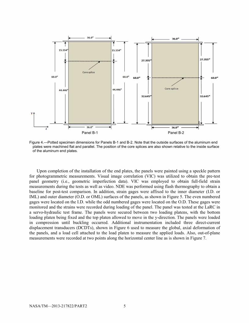
Panel B-1 Panel B-2 Figure 4.—Potted specimen dimensions for Panels B-1 and B-2. Note that the outside surfaces of the aluminum end

plates were machined flat and parallel. The position of the core splices are also shown relative to the inside surface of the aluminum end plates.

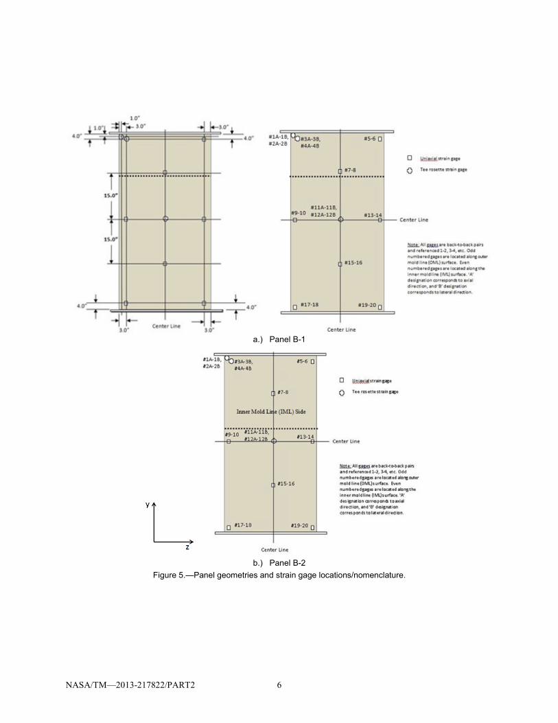
Upon completion of the installation of the end plates, the panels were painted using a speckle pattern

for photogrammetric measurements. Visual image correlation (VIC) was utilized to obtain the pre-test panel geometry (i.e., geometric imperfection data). VIC was employed to obtain full-field strain measurements during the tests as well as video. NDE was performed using flash thermography to obtain a baseline for post-test comparison. In addition, strain gages were affixed to the inner diameter (I.D. or IML) and outer diameter (O.D. or OML) surfaces of the panels, as shown in Figure 5. The even numbered gages were located on the I.D. while the odd numbered gages were located on the O.D. These gages were monitored and the strains were recorded during loading of the panel. The panel was tested at the LaRC in a servo-hydraulic test frame. The panels were secured between two loading platens, with the bottom loading platen being fixed and the top platen allowed to move in the y-direction. The panels were loaded in compression until buckling occurred. Additional instrumentation included three direct-current displacement transducers (DCDTs), shown in Figure 6 used to measure the global, axial deformation of the panels, and a load cell attached to the load platen to measure the applied loads. Also, out-of-plane measurements were recorded at two points along the horizontal center line as is shown in Figure 7.

NASA/TM—2013-217822/PART2 6

a.) Panel B-1

b.) Panel B-2

Figure 5.—Panel geometries and strain gage locations/nomenclature.

NASA/TM—2013-217822/PART2 7

Figure 6.—Location of DCDT’s on test machine platen.

Figure 7.—Location of DCDT’s on front (IML) surface of Panel B-1 and back

(OML) surface of Panel B-2.

3.0 Finite Element Analysis Description Pre-test predictions of the buckling loads for Panel B-1 and B-2 were determined using commercially

available FEM software packages: MSC/NASTRAN, Abaqus, and ANSYS. Figure 8 shows the test panel geometry used in the FE models. The panels were modeled as 60.00-in. tall (section between the aluminum end plates) and 35.60-in. along the arc (35.55-in. along the chord) using two-dimensional (2-D) layered shell elements. The shell models were offset so that the geometry corresponded to the OML. The 1.0 in. sections of the panels on the top and bottom that were supported in the potting material were not modeled. The element size was 1.00- by 0.97-in., and the models were comprised of 2257 nodes and 2160

DCDT on test machine platen

Top of load plate with potted test panel underneath

DCDTs on test machine platen

#1

#2 #3

Center Line

Center Line

DCDTs on front (IML) panel surface

#4

#5

NASA/TM—2013-217822/PART2 8

elements. All three displacements and all three rotations were fixed along the bottom edge of the panels. The same boundary condition was applied to the top edges, except a displacement was applied in the negative y-direction.

The stacking sequence of the facesheets was [60°/–60°/0°]s with 0.0053 in. plies. The IM7/977-3 elastic properties and allowables (used in strength analysis) were obtained from the Orion materials database, and are not shown as they are ITAR restricted (Lockheed Martin, 2010). The aluminum honeycomb properties were obtained from the database included with the commercially available structural sizing software, HyperSizer, and are presented in Table II. The in-plane normal and shear stiffnesses were reduced from 75.0 ksi to 1.00×10–7 ksi since in-plane load carrying capability of the honeycomb is typically neglected in honeycomb sandwich panel analysis.

Figure 8.—Panel geometry with boundary conditions.

TABLE II.—ALUMINUM HONEYCOMB

MATERIAL PROPERTIES, 3.1 pcf, 1/8 in.-5052-0.0007 E1, ksi ........................................................................... 1.00×10–7 E2, ksi ........................................................................... 1.00×10–7 ν12 ........................................................................................ 0.333 G12, ksi .......................................................................... 1.00×10–7 G1Z, ksi .................................................................................. 45.0 G2z, ksi ................................................................................... 22.0 ρ, pcf ..................................................................................... 3.10 Ft1, ksi .................................................................................... 0.20 Fc1, ksi ................................................................................... 0.20 Ft2, ksi .................................................................................... 0.20 Fc2, ksi ................................................................................... 0.20 Fs12, ksi .................................................................................. 0.09

NASA/TM—2013-217822/PART2 9

To arrive at the baseline buckling failure predictions, linear eigenvalue buckling analyses (Sol 105) were performed in MSC/NASTRAN. These preliminary analyses were completed for two reasons. First, the analyses provided reasonable estimates of what the non-linear analyses should predict as the panel buckling loads with an efficient, quick turnaround. Second, this is the typical method of calculating buckling loads for flight structures, and it is informative to compare the results to the experimental buckling loads and the buckling loads obtained from higher-fidelity models.

In addition, to improve numerical predictions, it was also pertinent to predict which direction (towards the I.D. or O.D.) the panels would buckle as a DCDT was to be placed to measure the out-of plane displacement of the panels and severe displacement in the unexpected direction would damage the gage. The eigenvectors obtained from an eigenvalue analysis are in an arbitrary direction and do not indicate the direction the panels would buckle. Therefore, geometrically non-linear static analyses were performed in MSC/NASTRAN (Sol 106), Abaqus, and ANSYS to arrive at more accurate buckling loads and determine the direction of buckling correctly.

Hause et al. (1998, 2000), Hilburger et al. (2001), Hilburger and Starnes, Jr. (2002), Lynch et al. (2004), Schultz and Nemeth (2010) have shown that FEM simulations of progressive collapse incorporating geometric non-linearities are extremely sensitive to the geometric imperfections in the panel. Thus, it was desired to use some measure of the actual imperfections of the panels and include them in the models. Preliminary photogrammetry data of the panel showed that the bag side (I.D.) surfaces contained some initial imperfections that were biased towards the I.D. On the O.D., or the tool side, the surface imperfections were sinusoidal in nature. Herein, these surface imperfections are referred to as the bow shapes of the panels. In the progressive collapse analyses, the bow data from the bag side of the panels was used to incorporate geometric imperfections into the model. Figure 9 shows the imperfection, or bow, data measured vertically from the top of the panels to the bottom of the panels at the horizontal center. The raw photogrammetry data was first rotated such that both the top and bottom had an out-of-plane bow displacement of 0.000 in. The data was then scaled (60 in./total height of photogrammetry data) so that it covered the full 60 in. of the panel. The approximated bow geometry was then swept along an arc of radius 198 in. and 10.272°, providing a uniform tangential panel cross section. Realistically, the cross section of the panel varies in the circumferential direction, but it was assumed that the imperfect, but uniform, cross section used in the numerical model is sufficient to capture the primary effects of the geometric imperfections in the panel. The imperfection data used to sweep the Panel B-1 model geometry is labeled “Avg IML Bow – MTP 6003” in Figure 9. The geometry of Panel B-2 was generated using the imperfection data labeled “Avg IML Bow – MTP 6000” in Figure 9. However, the response of the panel did not correlate with the expected panel buckling direction, and it was deemed that the data contained some erroneous scatter, especially near the bottom of the panel were the data show imperfection deflection towards the O.D. The Panel B-2 imperfection data was then approximated with a spline, shown in Figure 9 labeled as “Modified Spline Approximation – MTP 6000,” and data from this spline was used to sweep the geometry of the Panel B-2 model. All numerical results presented herein for Panel B-2 (MTP 6000) utilize the imperfection data obtained from the spline approximation of the measurements.

Finally, linear static solution in MSC/NASTRAN (Sol 101) was executed to determine the strength margins of safety at the time of onset of buckling. A similar analysis was performed in HyperSizer. These results were used to determine whether the failure of the panel was stiffness critical (buckling) or strength critical (local facesheet or core failure).

NASA/TM—2013-217822/PART2 10

Figure 9.—Imperfection, or bow, data from the bag side (I.D.) of the panel. Data were taken

vertically along the height of the panel, in the horizontal center of the panel.

Figure 10.—Method for determining

buckling load (Singer et al.,1998).

4.0 Test and Analysis Comparison To determine the panel buckling loads, a method from Singer, et al. (1998), shown in Figure 10, was

used. This method utilizes global load versus local strain gage data (axial strain) to mark the onset of buckling. In Figure 10, a vertical tangent line intersects the load-strain curve at a local strain where the local strain increment reverses which is designated the local buckling strain. The load corresponding to that local strain is designated the buckling load. It should be noted that the buckling strain, and hence buckling load, can only be determined at monitored locations and therefore can actually be lower than the lowest measured value. Thus, the postulated buckling load is somewhat subjective and based upon the location where the strains are being monitored for reversal. Test data for Gages 9 and 10 exhibited strain reversal at the lowest applied edge loads. These loads, 70,315 lb for Panel B-1 and 67,863 lb for Panel B-2, will be considered the buckling loads, and the numerical buckling loads will be determined from the global load versus local strain plots obtained from points on the models corresponding to these gage locations. It should be noted that for Panel B-1, the strain gages were monitored during the test, and the test was stopped upon apparent strain reversal in the gages to prevent and damage from arising in the panel.

-30

-20

-10

0

10

20

30

-0.01 0 0.01 0.02 0.03 0.04 0.05

Vert

ical

Loc

atio

n, in

.

Out-of-Plane Bow, in.

Avg IML Bow - MTP 6000Modified Spline Approximation - MTP 6000Avg IML Bow- MTP 6003

O.D. I.D.

NASA/TM—2013-217822/PART2 11

Panel B-1 Panel B-2 (Spline)

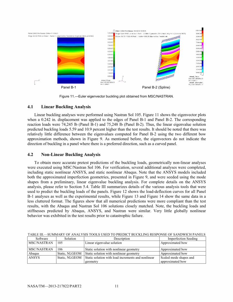
Figure 11.—Euler eigenvector buckling plot obtained from MSC/NASTRAN.

4.1 Linear Buckling Analysis

Linear buckling analyses were performed using Nastran Sol 105. Figure 11 shows the eigenvector plots when a 0.242 in. displacement was applied to the edges of Panel B-1 and Panel B-2. The corresponding reaction loads were 74,245 lb (Panel B-1) and 75,248 lb (Panel B-2). Thus, the linear eigenvalue solution predicted buckling loads 5.59 and 10.9 percent higher than the test results. It should be noted that there was relatively little difference between the eigenvalues computed for Panel B-2 using the two different bow approximation methods, shown in Figure 9. As mentioned before, the eigenvectors do not indicate the direction of buckling in a panel where there is a preferred direction, such as a curved panel.

4.2 Non-Linear Buckling Analysis

To obtain more accurate pretest predictions of the buckling loads, geometrically non-linear analyses were executed using MSC/Nastran Sol 106. For verification, several additional analyses were completed, including static nonlinear ANSYS, and static nonlinear Abaqus. Note that the ANSYS models included both the approximated imperfection geometries, presented in Figure 9, and were seeded using the mode shapes from a preliminary, linear eigenvalue buckling analysis. For complete details on the ANSYS analysis, please refer to Section 5.4. Table III summarizes details of the various analysis tools that were used to predict the buckling loads of the panels. Figure 12 shows the load-deflection curves for all Panel B-1 analyses as well as the experimental results, while Figure 13 and Figure 14 show the same data in a less cluttered format. The figures show that all numerical predictions were more compliant than the test results, with the Abaqus and Nastran Sol 106 solutions closely matched. Note, the buckling loads and stiffnesses predicted by Abaqus, ANSYS, and Nastran were similar. Very little globally nonlinear behavior was exhibited in the test results prior to catastrophic failure.

TABLE III.—SUMMARY OF ANALYSIS TOOLS USED TO PREDICT BUCKLING RESPONSE OF SANDWICH PANELS Software Solution Description Imperfection Seeding

MSC/NASTRAN 105 Linear eigenvalue solution Approximated bow

MSC/NASTRAN 106 Static solution with nonlinear geometry Approximated bow Abaqus Static, NLGEOM Static solution with nonlinear geometry Approximated bow ANSYS Static, NLGEOM Static solution with load increments and nonlinear

geometry Scaled mode shapes and approximated bow

NASA/TM—2013-217822/PART2 12

Figure 12.—Total Panel B-1 reaction load versus end shortening for all analyses.

Figure 13.—Total Panel B-1 reaction load versus end shortening for Sols 105,

106 and test.

NASA/TM—2013-217822/PART2 13

Figure 14.—Total Panel B-1 reaction load versus end shortening for Sols 105,

ANSYS, Abaqus, and test.

Figure 15.—DCDT end shortening versus total reaction load (Panel B-1).

In all the Panel B-1 (MTP-6003) analyses the linear pre-buckling panel stiffness was nearly the same.

However, the stiffness obtained from test results was higher than the analysis stiffness. Figure 15 shows the measurements of all three DCDTs that were affixed to the panel during loading. All three DCDTs showed higher stiffnesses, yielding an average measurement that produces a higher stiffness than the analytical predictions. Additionally, there is some initial non-linearity in the DCDT results due to initial settling, as expected. This indicates that there is some factor contributing to the stiffness of the panel that is not captured in the analyses. The slopes of the “NASTRAN SOL 106,” DCDT#1,” “DCDT#2,” “DCDT#3,” and “DCDT Specified Average” curves are presented in Table IV at an end shortening of 0.1 in. (to eliminate settling). Thus, additional sources of discrepancy between the stiffness of the FEM model and the experiment may be due to machine compliance, slight misalignments of the fibers within the plies

NASA/TM—2013-217822/PART2 14

to the intended ply angle, or variation in the fiber volume fraction/actual thickness of the plies resulting from the curing process. Results from a sensitivity study on fiber misalignment are presented in Section 5.2. In addition, results from a sensitivity study on 3-D effects using ANSYS are presented in Section 5.4.

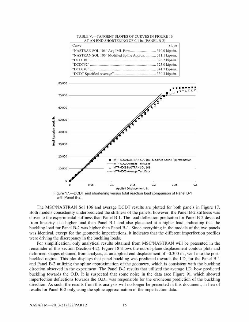
Figure 16 shows the experimental data obtained from the three DCDTs and the analytical predictions from Sol 105 and 106 using the average I.D. bow data, and the spline approximation of that data, for Panel B-2 (MTP-6000). Table V shows the slopes of the curves presented in Figure 16. There is relatively no difference in the slopes of the curves from Sol 106 analysis of Panel B-2 utilizing the two different bow approximation methods and Panel B-1, indicating the stiffness of the panel is relatively insensitive to geometric imperfections. The slopes from DCDT#1, DCDT#2 of Panel B-2 are closest to the analytical results, but the slope calculated using DCDT#3 is significantly higher. There was some slight misalignment of the test fixtures, as a maximum 5 percent difference in back-to-back strain gage measurements was permitted.

TABLE IV.—TANGENT SLOPES OF CURVES IN FIGURE 15 AT AN END SHORTENING OF 0.1 in. (PANEL B-1).

Curve Slope “NASTRAN SOL 106” .......................................... 306.2 kips/in. “DCDT#1” ............................................................. 338.0 kips/in. “DCDT#2” ............................................................. 333.0 kips/in. “DCDT#3” ............................................................. 334.6 kips/in. “DCDT Specified Average” ................................... 335.2 kips/in.

Figure 16.—DCDT end shortening versus total reaction load (Panel B-2).

NASA/TM—2013-217822/PART2 15

TABLE V.—TANGENT SLOPES OF CURVES IN FIGURE 16

AT AN END SHORTENING OF 0.1 in. (PANEL B-2) Curve Slope “NASTRAN SOL 106” Avg IML Bow ............................ 310.0 kips/in. “NASTRAN SOL 106” Modified Spline Approx. ........... 311.1 kips/in. “DCDT#1” ....................................................................... 326.2 kips/in. “DCDT#2” ....................................................................... 323.0 kips/in. “DCDT#3” ....................................................................... 341.7 kips/in. “DCDT Specified Average” ............................................. 330.3 kips/in.

Figure 17.—DCDT end shortening versus total reaction load comparison of Panel B-1

with Panel B-2. The MSC/NASTRAN Sol 106 and average DCDT results are plotted for both panels in Figure 17.

Both models consistently underpredicted the stiffness of the panels; however, the Panel B-2 stiffness was closer to the experimental stiffness than Panel B-1. The load deflection prediciton for Panel B-2 deviated from linearity at a higher load than Panel B-1 and also plateaued at a higher load, indicating that the buckling load for Panel B-2 was higher than Panel B-1. Since everything in the models of the two panels was identical, except for the geometric imperfections, it indicates that the different imperfection profiles were driving the discrepancy in the buckling loads.

For simplification, only analytical results obtained from MSC/NASTRAN will be presented in the remainder of this section (Section 4.2). Figure 18 shows the out-of-plane displacement contour plots and deformed shapes obtained from analysis, at an applied end displacement of –0.300 in., well into the post-buckled regime. This plot displays that panel buckling was predicted towards the I.D, for the Panel B-1 and Panel B-2 utilizing the spline approximation of the geometry, which is consistent with the buckling direction observed in the experiment. The Panel B-2 results that utilized the average I.D. bow predicted buckling towards the O.D. It is suspected that some noise in the data (see Figure 9), which showed imperfection deflections towards the O.D., was responsible for the erroneous prediction of the buckling direction. As such, the results from this analysis will no longer be presented in this document, in lieu of results for Panel B-2 only using the spline approximation of the imperfection data.

NASA/TM—2013-217822/PART2 16

Panel B-1

Panel B-2 (Spline)

Panel B-2 (Average I.D. Bow)

Figure 18.—Panel displacement plot.

NASA/TM—2013-217822/PART2 17

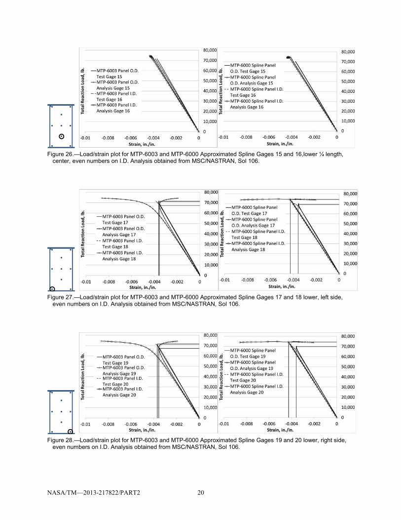
Table VI shows that the first strain reversal occurred at the location of gages 9 and 10, located at the center of the left edge of the panel (see Figure 5), at a load of 70,315 lb for Panel B-1 and 67,863 lb for Panel B-2. Loads corresponding to all strain gage locations are tabulated with the experimental values in Table VI. Figure 19 to Figure 21 show that, in the corner, the axial O.D. panel strains went into compression up to the onset of buckling, after which the strain increment reverses and the axial strain is alleviated as the load increases during post-buckling. This local behavior (observed both experimentally and numerically) is consistent as the panel buckled towards the I.D. Note that, since the major curvature of the panel is biased towards the O.D., the analysis would predict buckling towards the O.D. if no geometric imperfections (bow) were introduced into the model. Figure 22 shows the strain gage measurements at a panel inflection point at the ¾ panel length location. Figure 23 to Figure 25 shows that at the horizontal center of the panel, the I.D. panel strain goes into compression up to buckling and then starts reversing as the load increases during post-buckling. The results from Figure 26 the lower inflection or ¼ length location, match the results from Figure 22 while the results from Figure 27 and Figure 29 match the results from Figure 20 and Figure 21, respectively. The error in the nonlinear analyses ranges from 0.42 to 9.16 percent for Panel B-1 and 5.65 to 9.60 percent for Panel B-2 (Table VI), which was not much of an improvement over the linear analyses.

TABLE VI.—APPROXIMATE TEST AND ANALYSIS PREDICTION BUCKLING LOADS [See Figure 5 for gage locations on panel]

Gage Test, lb (Panel B-1/Panel B-2)

Analysis, lb (Panel B-1/Panel B-2)

Percent error (Panel B-1/Panel B-2)

1,2 70,397/70,171 70,097/74,134 0.42/5.65 3,4 71,283/69,470 68,321/74,314 4.16/6.97 5,6 71,057/69,100 68,321/74,314 3.85/7.55

9,10 70,315/67,863 64,118/74,375 8.81/9.60 11,12 71,448/68,543 66,283/74,375 7.23/8.51 13,14 70,583/69,100 64,118/74,544 9.16/7.88 17,18 71,036/69,285 68,321/74,314 3.82/7.26 19,20 71,139/69,841 68,321/74,314 3.96/6.40

Figure 19.—Load/strain plot for MTP-6003 and MTP-6000 Approximated Spline Gages 1 and 2 upper, left side, even

numbers on I.D. Analysis obtained from MSC/NASTRAN, Sol 106.

NASA/TM—2013-217822/PART2 18

Figure 20.—Load/strain plot for MTP-6003 and MTP-6000 Approximated Spline Gages 3 and 4, upper, left side, even

numbers on I.D. Analysis obtained from MSC/NASTRAN, Sol 106.

Figure 21.—Load/strain plot for MTP-6003 and MTP-6000 Approximated Spline Gages 5 and 6,upper, right side,

even numbers on I.D. Analysis obtained from MSC/NASTRAN, Sol 106.

Figure 22.—Load/strain plot for MTP-6003 and MTP-6000 Approximated Spline Gages 7 and 8, upper ¼ length,

center, even numbers on I.D. Analysis obtained from MSC/NASTRAN, Sol 106.

NASA/TM—2013-217822/PART2 19

Figure 23.—Load/strain plot for MTP-6003 and MTP-6000 Approximated Spline Gages 9 and 10,center, left side,

even numbers on I.D.. Analysis obtained from MSC/NASTRAN, Sol 106.

Figure 24.—Load/strain plot for MTP-6003 and MTP-6000 Approximated Spline Gages 11 and 12,center of panel,


Figure 25.—Load/strain plot for MTP-6003 and MTP-6000 Approximated Spline Gages 13 and 14 center, left side,


NASA/TM—2013-217822/PART2 20

Figure 26.—Load/strain plot for MTP-6003 and MTP-6000 Approximated Spline Gages 15 and 16,lower ¼ length,

center, even numbers on I.D. Analysis obtained from MSC/NASTRAN, Sol 106.

Figure 27.—Load/strain plot for MTP-6003 and MTP-6000 Approximated Spline Gages 17 and 18 lower, left side,


Figure 28.—Load/strain plot for MTP-6003 and MTP-6000 Approximated Spline Gages 19 and 20 lower, right side,


NASA/TM—2013-217822/PART2 21

The non-linear MSC Nastran Sol 106 analysis full field results are compared qualitatively with the test results. Since both panels exhibited the same qualitative response, strain contours are only presented here for Panel B-1. Figure 29 shows that the post-buckled, in-plane displacement photogrammetry results qualitatively compared well with the analytical predictions. Since shell elements were used in the analysis, the nodal displacements do not vary on the O.D. and I.D. surfaces, whereas, the test results showed some slight variation in displacement for the I.D. and O.D. surfaces due to the finite width of the panel. Figure 30 shows the evolution of the in-plane displacement, obtained from the numerical analysis, as the applied compressive load is increased. Figure 31 shows that the post-buckled, out-of plane, displacement also compared well qualitatively with the analytical predictions. Figure 32 shows that the out-of-plane displacement was negligible up to the load of 74,358 lb.

Figure 29.—Post-buckling Y (in-plane) displacement comparison.

Figure 30.—Analytical Y (in-plane) displacement.

NASA/TM—2013-217822/PART2 22

For the O.D. surface, Figure 33 and Figure 34 show the minimum principal strain test results did not compare well with the analytical predictions. This may indicate that the test panel was not loaded high enough for the minimum principle strains to fully develop in the post-buckled regime. Like the out-of-plane displacement, the minimum principal strains, from the analysis, were negligible up until post-buckling. For the I.D. surface, Figure 35 and Figure 36 show that the minimum principal strain also did not compare well. Figure 37 to Figure 40 show the maximum principal strain comparisons. Again, it appears that the photogrammetric strains do not fully develop in the post-buckled state, and that the applied loading during the experiment may have needed to be taken to a slightly higher value.

Figure 31. Post-buckling X (out-of-plane) displacement comparison.

Figure 32.—Analytical X (out-of-plane) displacement.

NASA/TM—2013-217822/PART2 23

Figure 33.—Post-buckling O.D. minimum principal (Y) strain comparison.

Figure 34.—Analytical minimum principal strain (Y) strain O.D.

NASA/TM—2013-217822/PART2 24

Figure 35.—Post-buckling I.D. minimum principal (Y) strain comparison

Figure 36.—Analytical minimum principal strain (Y) strain I.D.

NASA/TM—2013-217822/PART2 25

Figure 37.—Post-buckling O.D. maximum principal (Z) strain comparison.

Figure 38.—Analytical maximum principal strain (Z) strain O.D.

NASA/TM—2013-217822/PART2 26

Figure 39.—Post-buckling I.D. maximum principal (Z) strain comparison.

Figure 40.—Analytical maximum principal strain (Z) strain I.D.

NASA/TM—2013-217822/PART2 27

4.3 Strength Analysis at Buckling Load

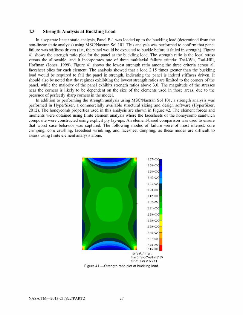
In a separate linear static analysis, Panel B-1 was loaded up to the buckling load (determined from the non-linear static analysis) using MSC/Nastran Sol 101. This analysis was performed to confirm that panel failure was stiffness driven (i.e., the panel would be expected to buckle before it failed in strength). Figure 41 shows the strength ratio plot for the panel at the buckling load. The strength ratio is the local stress versus the allowable, and it incorporates one of three multiaxial failure criteria: Tsai-Wu, Tsai-Hill, Hoffman (Jones, 1999). Figure 41 shows the lowest strength ratio among the three criteria across all facesheet plies for each element. The analysis showed that a load 2.15 times greater than the buckling load would be required to fail the panel in strength, indicating the panel is indeed stiffness driven. It should also be noted that the regimes exhibiting the lowest strength ratios are limited to the corners of the panel, while the majority of the panel exhibits strength ratios above 3.0. The magnitude of the stresses near the corners is likely to be dependent on the size of the elements used in those areas, due to the presence of perfectly sharp corners in the model.

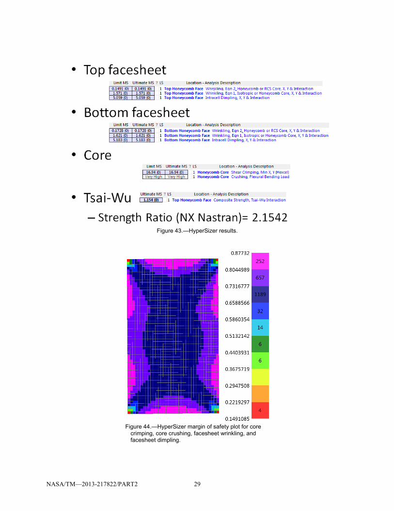
In addition to performing the strength analysis using MSC/Nastran Sol 101, a strength analysis was performed in HyperSizer, a commercially available structural sizing and design software (HyperSizer, 2012). The honeycomb properties used in this analysis are shown in Figure 42. The element forces and moments were obtained using finite element analysis where the facesheets of the honeycomb sandwich composite were constructed using explicit ply lay-ups. An element-based comparison was used to ensure that worst case behavior was captured. The following modes of failure were of most interest: core crimping, core crushing, facesheet wrinkling, and facesheet dimpling, as these modes are difficult to assess using finite element analysis alone.

Figure 41.—Strength ratio plot at buckling load.

NASA/TM—2013-217822/PART2 28

Figure 42.—Honeycomb Hexcel core properties.

Figure 43 shows that all the margins are positive for core crimping, core crushing, facesheet

wrinkling, and facesheet dimpling. It should be noted that the minimum strength ratios (margin of safety plus one) from Nastran and HyperSizer matched very well, both indicated a strength ratio of 2.15. It was determined that the wrinkling equations used to produce the margin of safety contour plot (with a minimum margin of safety of 0.149) in Figure 44 were not appropriate for a honeycomb sandwich panel with laminated composite facesheets (Zalewski et al., 2012). Therefore, wrinkling stress (sw) was assessed using the wrinkling Equation (1) (where tf is the facesheet thickness, tc is the core thickness, Ef is the facesheet modulus, Ec is the core modulus, and υf is the facesheet Poisson’s ratio) for anisotropic facesheets and cellular core (Vinson, 1999), as is more appropriate for this panel. To improve the accuracy the wrinkling margin of safety, a combined loading condition was used, Equation (2), with two compressive principal stresses (Ley et al., 1999). Using this more appropriate method, the minimum margin of safety further increased from 0.149 to 0.963. Thus, it was predicted that facesheet wrinkling in the corners of the panel would not be an issue, and the experimental data presented in Figure 19 supports this assumption.

( )2132

=fc

fcf

υtEEt

sw−

(1)

1σσ

1=MOS2

31

−

+

swsw

(2)

NASA/TM—2013-217822/PART2 29

Figure 43.—HyperSizer results.

Figure 44.—HyperSizer margin of safety plot for core

crimping, core crushing, facesheet wrinkling, and facesheet dimpling.

NASA/TM—2013-217822/PART2 30

5.0 Sensitivity Studies 5.1 Sensitivity to Panel Geometry

The analyses presented in Section 4.2 utilized geometric imperfection data from the panel measured vertically along a single horizontal coordinate. It is very likely, that if a different location was chosen to measure this data, the bow shape, and maximum imperfection would have been different. The results presented in Section 4.2 indicate that the buckling load and direction of these curved panels are very sensitive to the geometric imperfections contained in the panel. To investigate the imperfection sensitivity further, a parametric study was conducted incorporating various levels of bow imperfection. A regular arc shape was assumed with the maximum deflection towards the I.D. being located at the vertical center of the panel. This bow shape was then swept horizontally to arrive at the full geometry of the panel. The maximum bow deflection was varied from 0.01 to 0.04 in.

Previous studies showed that the geometric imperfections had a negligible effect on the stiffness of the panel (Myers et al., 2013). The buckling loads obtained using the various levels of imperfection are plotted in Figure 45, along with the test results and the numerical predictions utilizing approximations of the actual imperfection data. As the maximum bow deflection (towards the I.D.) increased from 0.010 to 0.017 in., the buckling load increased 72,340 to 76,220 lb. As the maximum bow deflection is increased

Figure 45.—Impact of initial panel bow geometry on panel buckling loads.

NASA/TM—2013-217822/PART2 31

beyond 0.017 in., the buckling load started to decrease. It should also be noted that when the bow was 0.017 in. or less, the panel buckled towards O.D., but when the bow was greater than 0.017 in., the panel buckled towards the I.D. Thus, a geometric imperfection (in the shape of a swept arc) with a maximum deflection of 0.017 in. represents a transition point beyond which the direction of buckling switches. This is consistent with a similar study performed by Myers et al. (2013) for a similar panel with 8-ply facesheets composed of the same material. As the bow gets closer to this transition point, an increase in the bow deflection helps to resist buckling because the bow direction is opposite the buckling direction. Beyond this transition point, an increase in the bow deflection acts to aid the buckling because the buckling direction and bow deflection are the same.

The Panel B-1 and Panel B-2 simulations presented in Section 4.2 utilized bow shapes that contained maximum deflections beyond the 0.017 in. threshold. The predictions from these models followed a similar trend to that observed in the bow study. The buckling load prediction from the Panel B-2 model, for which the bow was modeled using a spline approximation, matched very closely with the corresponding buckling load from the bow study. However, the Panel B-1 prediction was significantly lower than the bow study prediction that incorporated the same maximum bow deflection. The imperfection geometry utilized in the Panel B-1 model was composed of the averaged imperfection data measured from the panel and did not conform to a regular shape (such as the spline approximation). This signifies that both maximum bow deflection and shape may influence the prediction results.

The experimental buckling loads did not follow the same trend as the bow study. This may imply that the full field imperfections are needed to predict the response of the panel accurately. However, there is a discrepancy in the stiffness of the panels (see Figure 17) which cannot be reproduced by incorporating imperfections (Myers et al., 2013). Moreover, it is other imperfections that are contributing to the discrepancies observed in the buckling loads and stiffnesses between the experimental data and analytical predictions.

5.2 60° Ply Fiber Misalignment Sensitivity Study

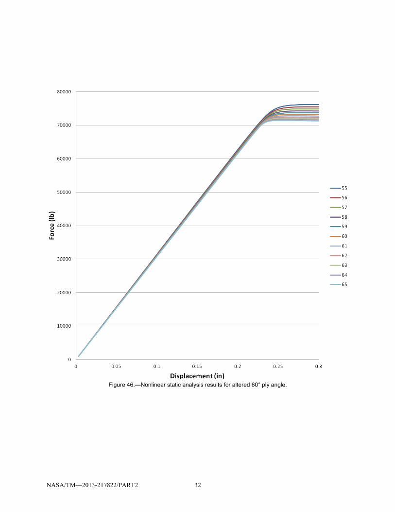
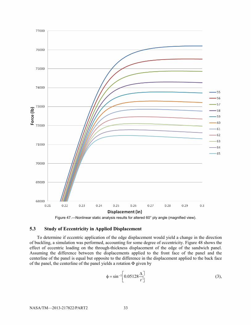
For this study, the Panel B-1 model as described in Section 3.0 was used; however, the orientation of the 60° plies was varied from 55° to 65° in increments of 1°. The 0° plies were not altered as it was assumed that their orientation does not vary during the ply lay-up process. Nastran Sol 106 was used to analyze the panel. Figure 46 shows the force-displacement results from the orientation variation study, and Figure 47 shows a magnified view of the plot near the region where the load plateaus. These figures show that the plateau load, and by extension the buckling load, predicted by the model can be significantly affected by plus/minus 5° of misalignment in the plies. Although, there is some change in the stiffness as a function of misalignment, the effect is minimal, and most likely, not the reason for the large discrepancy in stiffness observed between the experiment and the analytical results. An input from FiberSim would better model the true fiber alignment.

NASA/TM—2013-217822/PART2 32

Figure 46.—Nonlinear static analysis results for altered 60° ply angle.

NASA/TM—2013-217822/PART2 33

Figure 47.—Nonlinear static analysis results for altered 60° ply angle (magnified view).

5.3 Study of Eccentricity in Applied Displacement

To determine if eccentric application of the edge displacement would yield a change in the direction of buckling, a simulation was performed, accounting for some degree of eccentricity. Figure 48 shows the effect of eccentric loading on the through-thickness displacement of the edge of the sandwich panel. Assuming the difference between the displacements applied to the front face of the panel and the centerline of the panel is equal but opposite to the difference in the displacement applied to the back face of the panel, the centerline of the panel yields a rotation Φ given by

∆

=φ −

t05128.0sin 1 (3),

NASA/TM—2013-217822/PART2 34

where Δ is the centerline displacement and t is the total thickness of the panel. The angle Φ is applied to the edge of the panel in the shell model as a rotation to simulate a through-thickness eccentricity in the applied edge displacement in the experiment. The angle used in the simulation is 20 percent of the buckling displacement from the linear eigenvalue solution and is calculated to be 0.12° using Equation (3). It is assumed that this level of eccentricity is present from the beginning of the analysis and is constant throughout the duration of the simulation.

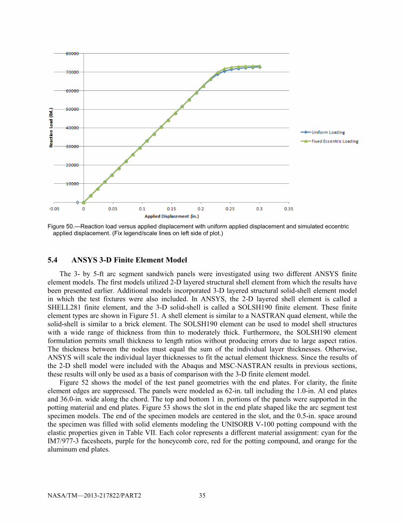
Figure 49 shows the post-buckled shapes predict using a non-linear analysis with a uniform edge displacement an edge displacement with eccentricity corresponding to a rotation of 0.12°. Figure 50 shows a comparison in the load-deflection behavior from the two simulations. These two figures show that the buckling direction and the quantitative response of the panel is largely unaffected by the assumed misalignment.

Figure 48.—Diagram showing eccentric

loading applied through the thickness of the panel leading to rotation of the panel edge.

Figure 49.—Post-buckled shape with uniform applied displacement and

simulated eccentric applied displacement.

NASA/TM—2013-217822/PART2 35

Figure 50.—Reaction load versus applied displacement with uniform applied displacement and simulated eccentric

applied displacement. (Fix legend/scale lines on left side of plot.)

5.4 ANSYS 3-D Finite Element Model

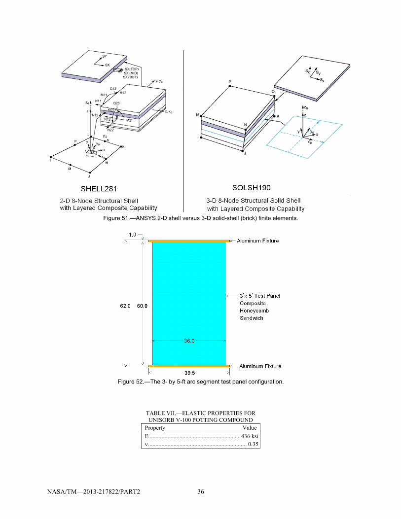
The 3- by 5-ft arc segment sandwich panels were investigated using two different ANSYS finite element models. The first models utilized 2-D layered structural shell element from which the results have been presented earlier. Additional models incorporated 3-D layered structural solid-shell element model in which the test fixtures were also included. In ANSYS, the 2-D layered shell element is called a SHELL281 finite element, and the 3-D solid-shell is called a SOLSH190 finite element. These finite element types are shown in Figure 51. A shell element is similar to a NASTRAN quad element, while the solid-shell is similar to a brick element. The SOLSH190 element can be used to model shell structures with a wide range of thickness from thin to moderately thick. Furthermore, the SOLSH190 element formulation permits small thickness to length ratios without producing errors due to large aspect ratios. The thickness between the nodes must equal the sum of the individual layer thicknesses. Otherwise, ANSYS will scale the individual layer thicknesses to fit the actual element thickness. Since the results of the 2-D shell model were included with the Abaqus and MSC-NASTRAN results in previous sections, these results will only be used as a basis of comparison with the 3-D finite element model.

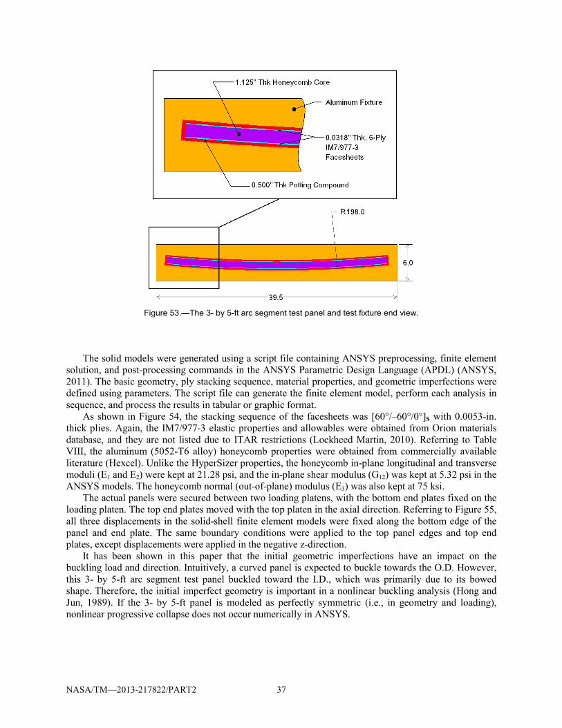
Figure 52 shows the model of the test panel geometries with the end plates. For clarity, the finite element edges are suppressed. The panels were modeled as 62-in. tall including the 1.0-in. Al end plates and 36.0-in. wide along the chord. The top and bottom 1 in. portions of the panels were supported in the potting material and end plates. Figure 53 shows the slot in the end plate shaped like the arc segment test specimen models. The end of the specimen models are centered in the slot, and the 0.5-in. space around the specimen was filled with solid elements modeling the UNISORB V-100 potting compound with the elastic properties given in Table VII. Each color represents a different material assignment: cyan for the IM7/977-3 facesheets, purple for the honeycomb core, red for the potting compound, and orange for the aluminum end plates.

NASA/TM—2013-217822/PART2 36

Figure 51.—ANSYS 2-D shell versus 3-D solid-shell (brick) finite elements.

Figure 52.—The 3- by 5-ft arc segment test panel configuration.

TABLE VII.—ELASTIC PROPERTIES FOR UNISORB V-100 POTTING COMPOUND

Property Value E ............................................................. 436 ksi ν .................................................................. 0.35

NASA/TM—2013-217822/PART2 37

Figure 53.—The 3- by 5-ft arc segment test panel and test fixture end view.

The solid models were generated using a script file containing ANSYS preprocessing, finite element

solution, and post-processing commands in the ANSYS Parametric Design Language (APDL) (ANSYS, 2011). The basic geometry, ply stacking sequence, material properties, and geometric imperfections were defined using parameters. The script file can generate the finite element model, perform each analysis in sequence, and process the results in tabular or graphic format.

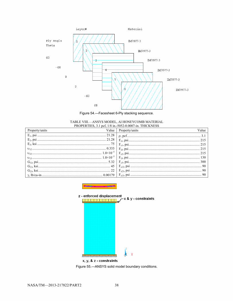
As shown in Figure 54, the stacking sequence of the facesheets was [60°/–60°/0°]S with 0.0053-in. thick plies. Again, the IM7/977-3 elastic properties and allowables were obtained from Orion materials database, and they are not listed due to ITAR restrictions (Lockheed Martin, 2010). Referring to Table VIII, the aluminum (5052-T6 alloy) honeycomb properties were obtained from commercially available literature (Hexcel). Unlike the HyperSizer properties, the honeycomb in-plane longitudinal and transverse moduli (E1 and E2) were kept at 21.28 psi, and the in-plane shear modulus (G12) was kept at 5.32 psi in the ANSYS models. The honeycomb normal (out-of-plane) modulus (E3) was also kept at 75 ksi.

The actual panels were secured between two loading platens, with the bottom end plates fixed on the loading platen. The top end plates moved with the top platen in the axial direction. Referring to Figure 55, all three displacements in the solid-shell finite element models were fixed along the bottom edge of the panel and end plate. The same boundary conditions were applied to the top panel edges and top end plates, except displacements were applied in the negative z-direction.

It has been shown in this paper that the initial geometric imperfections have an impact on the buckling load and direction. Intuitively, a curved panel is expected to buckle towards the O.D. However, this 3- by 5-ft arc segment test panel buckled toward the I.D., which was primarily due to its bowed shape. Therefore, the initial imperfect geometry is important in a nonlinear buckling analysis (Hong and Jun, 1989). If the 3- by 5-ft panel is modeled as perfectly symmetric (i.e., in geometry and loading), nonlinear progressive collapse does not occur numerically in ANSYS.

NASA/TM—2013-217822/PART2 38

Figure 54.—Facesheet 6-Ply stacking sequence.

TABLE VIII.—ANSYS MODEL, Al HONEYCOMB MATERIAL

PROPERTIES, 3.1 pcf, 1/8 in.-5052-0.0007-in. THICKNESS Property/units Value Property/units Value E1, psi ............................................................................... 21.28 E2, psi ............................................................................... 21.28 E3, ksi .................................................................................... 75 υ12 ..................................................................................... 0.333 υ23 ................................................................................ 1.0×10–5 υ13 ................................................................................ 1.0×10–5 G12, psi ................................................................................ 5.32 G13, ksi ................................................................................... 45 G23, ksi ................................................................................... 22 γ, lb/cu-in ...................................................................... 0.00179

ρ, pcf ..................................................................................... 3.1 Ft1, psi .................................................................................. 215 Fc1, psi.................................................................................. 215 Ft2, psi .................................................................................. 215 Fc2, psi.................................................................................. 215 Ft3, psi .................................................................................. 130 Fc3, psi.................................................................................. 300 Fs12, psi .................................................................................. 90 Fs23, psi .................................................................................. 90 Fs13, psi .................................................................................. 90

Figure 55.—ANSYS solid model boundary conditions.

NASA/TM—2013-217822/PART2 39

One way to introduce anti-symmetry to the model is to apply small perturbations to the applied loads or enforced displacements. This method is not ideal, because it is difficult to determine how to redistribute the loads. Furthermore, varying the load across the top of the panel too drastically could change the problem completely. Another way to introduce anti-symmetry is to superimpose small geometric imperfections (similar to those caused by manufacturing) on the model to trigger the buckling responses. One way to generate these imperfections is with pseudo-random shapes, where the coordinates of the nodes are slightly modified with random amplitudes. The disadvantage in using random imperfections is that they cannot be repeated, and the results would differ for each analysis of the same panel. An easier way to impose geometric imperfections on the finite element model is to employ the linear (Eigen) buckling mode shapes.

The buckling analysis of the 3- by 5-ft arc-segment panel requires several steps. First, the initial bow shape is imposed across the width of the panel model. The imperfections are obtained by running a preliminary linear buckling analysis, then updating the geometry of the finite element model to the deformed configuration. This technique is done by adding the displacements from the mode shapes multiplied by a scaling factor. The scaling factor is on the order of the manufacturing tolerances and initial bowed shape. A factor of –0.020 in. was chosen for the 3- by 5-ft panel. Furthermore, the scaling factor was negative to correspond to the direction of the initial bow shape. Applying a positive value could bring the panel model back to a near perfect condition. The imperfections are also added as a sum of the first 10 modes shapes extracted in the preliminary linear buckling analysis as shown in Figure 56. The first 10 mode shapes were used to avoid any bias in the imperfections. Figure 57 shows the resulting geometry for Panel B-1. The same procedure was used to generate the geometry for Panel B-2 using the measured imperfections and mode shapes.

Figure 56.—The first 10 linear buckling mode shapes for the 3 by 5 panel with 6-ply facesheets.

NASA/TM—2013-217822/PART2 40

Figure 57.—Panel B-1 model with the applied initial bowed

shape and geometric imperfections (exaggerated). After the geometric imperfections are added to the finite element model, the nonlinear buckling

analysis is performed. In ANSYS, a nonlinear buckling analysis is a static analysis with large deflections active. The magnitude of the applied axial compression is extended beyond the first linear (Eigen) buckling mode. In this analysis the compression was increased gradually using 50 small time increments to predict the critical buckling load.

Figure 58 shows the reaction load versus end compression for the linear and nonlinear shell and solid ANSYS models and the actual test data of Panel B-1. The two linear buckling analyses over-predicted the buckling load, but the two nonlinear analyses under-predicted the buckling load. The nonlinear shell FEM is closest to the test result buckling load. In both nonlinear ANSYS analyses, the panel stiffness was nearly the same. However, the predicted stiffnesses were lower than the test stiffness. Reasons for the difference in stiffness were discussed earlier.

Figure 61 shows the reaction load versus end compression for the linear and nonlinear shell and solid ANSYS models and the actual test data of Panel B-2. Note that, the maximum test value does not necessarily correspond to the experimental buckling load, rather local strain gage data must be used to assess the buckling load. The two linear buckling analyses over-predicted the buckling load, but the two nonlinear analyses just slightly over-predict the buckling load. The nonlinear solid FEM is closest to the test result buckling load. In both nonlinear ANSYS analyses, the panel stiffness was nearly the same. However, the predicted stiffnesses were only lower than test stiffness as recorded by one DCDT. The predicted stiffnesses were in closer agreement with the other two DCDT's.

Figure 59 and Figure 62 show the panel radial displacement plot (radial component of the total displacement field) when –0.21888 in. was applied to the top edge. As explained earlier, Figure 59 shows the panel buckles in towards the I.D. due to the initial bow and not in the direction of the panel’s outer surface. The plot also shows asymmetry in the radial displacements which is also evident in the buckling predictions shown in Table IX. The asymmetry in the radial displacements of Figure 59 and Figure 62 is due to the asymmetry in some of the linear buckling mode shapes (as shown in Figure 56) which were superimposed on the original geometry. The difference in the radial displacement contours is due to the

NASA/TM—2013-217822/PART2 41

difference in the initial bow shapes of Panel B-1 and B-2 (see Figure 9). The differences in these radial displacements demonstrate the sensitivity of the buckling analysis and resulting loads to the initial geometric imperfections. Thus, imperfections must be accounted for accurately in the modeling if they are significant compared to the overall dimension of the panel.

Figure 60 and Figure 63 show load versus strain plots for gages located in the center of the panel. On the I.D. side of the panel, the strain goes into compression up to buckling and then starts relieving itself as the load increases during post-buckling. On the O.D. side, the strain remains compressive (negative) and suddenly increases in magnitude during post-buckling. The analysis results for the ANSYS shell and solid FEM's show the same trends in strain at that gage location.

Figure 58.—Total reaction load versus end shortening for ANSYS solid and shell FEMs of panel B-1.

TABLE IX.—APPROXIMATE TEST AND ANALYSIS PREDICTION BUCKLING LOADS

Gage Test, lb (Panel B-1/Panel B-2)

Analysis, lb (Panel B-1/Panel B-2)

Percent error (Panel B-1/Panel B-2)

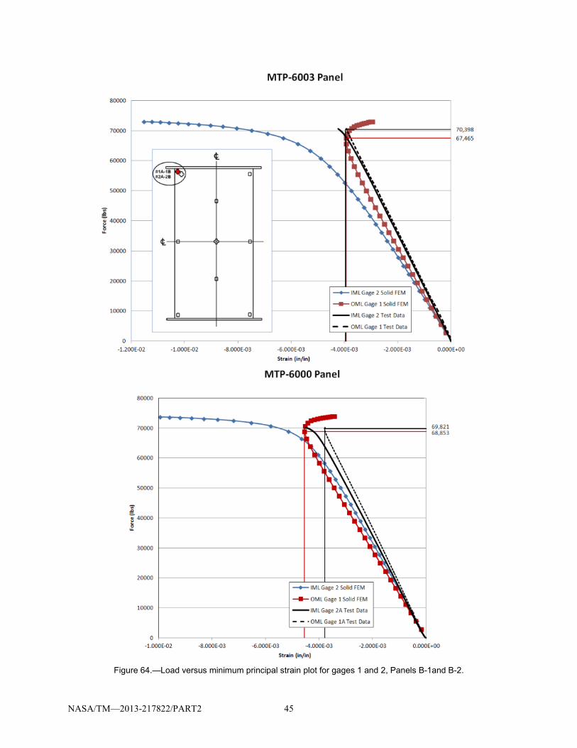
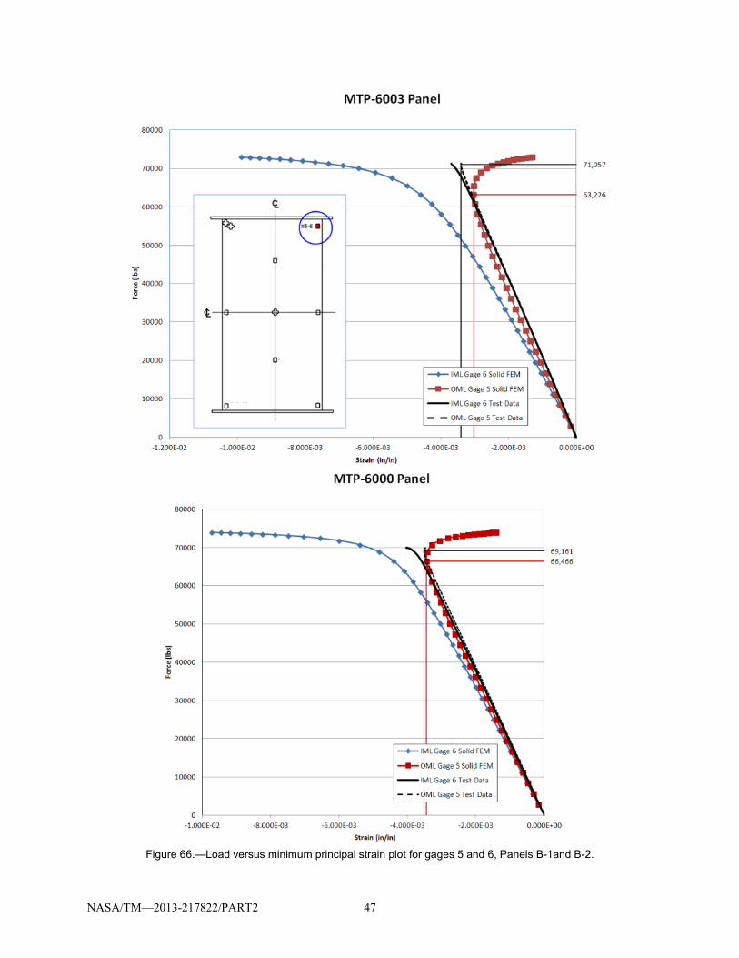
1,2 70,398 / 69,821 67,465 / 68,853 4.17 / 1.39 3,4 71,222 / 69,326 63,226 / 66,466 11.23 / 4.13 5,6 71,057 / 69,161 63,226 / 66,466 11.02 / 3.90

9,10 70,315 / 67,863 60,714 / 63,835 13.65 / 5.94 11,12 71,243 / 68,543 63,226 / 66,466 11.25 / 3.03 13,14 70,233 / 68,543 58,086 / 63,835 17.30 / 6.87 17,18 71,057 / 69,264 65,524 / 66,466 7.79 / 4.04 19,20 71,140 / 69,388 63,226 / 66,466 11.12 / 4.21

NASA/TM—2013-217822/PART2 42

Figure 59.—ANSYS solid FEM, radial displacement contour plot for Panel B-

1 at 0.219-in. end shortening.

Figure 60.—Load versus minimum principal strain plots for Panel B-1 at gages 11 and 12.

ANSYS 14.0FEB 19 201316:43:33PLOT NO. 2NODAL SOLUTIONSTEP=1SUB =24TIME=.48UXMIDDLELAYR=6RSYS=1DMX =.355216SMN =-.33274SMX =.701E-03

1

MN

MX

Global Radial Displacement Contours

Geometric ImperfectionsScale Factor = -.02

X Y

Z

-.33274-.295691-.258642-.221593-.184544-.147495-.110446-.073397-.036348.701E-03

3x5 Coupon, 6-ply, IM7/977-3, Face Sheets, Bowed, -0.21888" Disp

NASA/TM—2013-217822/PART2 43

Figure 61.—Total reaction load versus end shortening for ANSYS solid and shell FEM's of Panel B-2.

Figure 62.—ANSYS solid FEM, radial displacement contour plot for Panel B-2 at 0.219-in. end shortening.

ANSYS 14.0DEC 31 201211:28:28PLOT NO. 2NODAL SOLUTIONSTEP=1SUB =24TIME=.48UXMIDDLELAYR=6RSYS=1DMX =.221086SMN =-.187266SMX =.001174

1

MN

MX

Global Radial Displacement Contours

Geometric ImperfectionsScale Factor = -.02

X Y

Z

-.187266-.166328-.14539-.124453-.103515-.082577-.061639-.040702-.019764.001174

3x5 Coupon, 6-ply, IM7/977-3, Face Sheets, Bowed, -0.21888" Disp

NASA/TM—2013-217822/PART2 44

Figure 63.—Load versus minimum principal strain plot for Panel B-2 at gages 11 and 12.

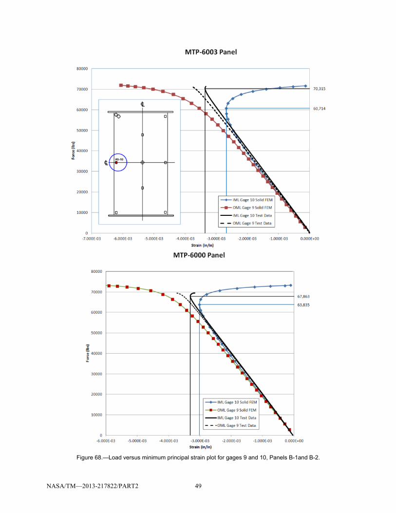
Table IX shows that the first strain reversal occurred at the location of gages 13 and 14, located at the

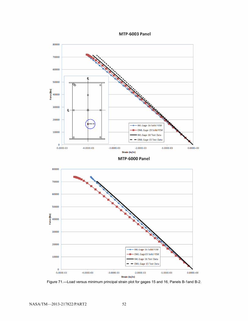
center of the right edge of the panel, at a load of 70,233 lb for Panel B-1 and at gages 9 and 10 at 67,863 lb for Panel B-2. Loads corresponding to all strain gage locations are tabulated with the experimental values in Table IX. Note that the experimental values differ slightly from those in Table VI. This is attributed to minor variations in the methodologies used to reduce the data. Figure 64 to Figure 66 show that, in the corners, the axial O.D. (OML) panel strains went into compression up to the onset buckling, after which the strain increment reverses and the axial strain is alleviated as the load increases during post-buckling. As pointed out earlier in this paper, this local behavior (observed both experimentally and numerically) is consistent as the panel buckled towards the I.D. Note that, since the major curvature of the panel is biased towards the O.D., the analysis would predict buckling towards the O.D. if no geometric imperfections (or bow) were introduced into the model. Figure 67 shows the strain gage measurements at a panel inflection point at the ¾ panel length location. Figure 68 to Figure 70 show that at the horizontal center of the panel, the I.D. (IML) panel strain goes into compression up to buckling and then reverses as the load increases during post-buckling. The results from Figure 71 the lower inflection or ¼ length location, match the results from Figure 67. The results in the lower corners from Figure 72 and Figure 73 match the results from the upper corners in Figure 65 and Figure 66, respectively. The error in the nonlinear analyses ranges from 4.17 to 17.3 percent for Panel B-1 and 1.39 to 6.87 percent for Panel B-2 (Table IX), which was not much of an improvement over the linear analyses.

NASA/TM—2013-217822/PART2 45

Figure 64.—Load versus minimum principal strain plot for gages 1 and 2, Panels B-1and B-2.

NASA/TM—2013-217822/PART2 46


NASA/TM—2013-217822/PART2 47


NASA/TM—2013-217822/PART2 48


NASA/TM—2013-217822/PART2 49


NASA/TM—2013-217822/PART2 50


NASA/TM—2013-217822/PART2 51


NASA/TM—2013-217822/PART2 52


NASA/TM—2013-217822/PART2 53


NASA/TM—2013-217822/PART2 54


NASA/TM—2013-217822/PART2 55

Since both panels exhibited the same qualitative response, displacement and strain contours are only presented here for Panel B-1. Figure 74 shows that the post-buckled, in-plane or longitudinal displacement photogrammetry results qualitatively compared well with the analytical predictions. In the ANSYS solid element model, the nodal displacements do not vary on the O.D. and I.D. surfaces, whereas, the test results showed some slight variation in displacement for the I.D. and O.D. surfaces due to the finite width of the panel. Figure 75 shows the evolution of the in-plane or longitudinal displacement, obtained from the numerical analysis, as the applied compressive load is increased. Figure 76 shows that the post-buckled, out-of plane or radial, displacement also compared well qualitatively with the analytical predictions. Figure 77 shows that the out-of-plane displacement was negligible up to the load of 70,001 lb.

Figure 74.—Post-buckling Z (in-plane or longitudinal) displacement comparison

for Panel B-1.

Figure 75.—ANSYS solid FEM axial (Z-axis or longitudinal) displacement contour plots versus load for Panel B-1.

NASA/TM—2013-217822/PART2 56

Figure 76.—Post-buckling X (out-of-plane or radial) displacement

comparison for Panel B-1.

Figure 77.—ANSYS solid FEM out-of-plane (X-axis or radial) displacement contour plots versus load for Panel B-1.

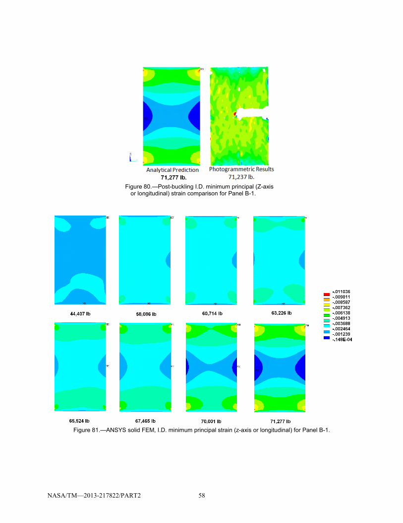
For the O.D. surface, Figure 78 shows that the post-buckled, minimum principal strain test results did not compare well with the analytical; however, both show most of the strain developing in the center of the panel. Like the out-of-plane displacement, the minimum principal strain (compressive) was uniform up until the point of buckling, as shown in Figure 79. For the I.D. surface, Figure 80 shows that the minimum principal strain also did not compare perfectly, and shows the predicted progression of the minimum principal strain from the analysis. Figure 81 shows the minimum principal strain (compressive) on the I.D. surface was uniform up until the point of buckling. The minimum principal strain was the

NASA/TM—2013-217822/PART2 57

primary strain in the buckling test. The magnitudes of the maximum principal strains were very low, thus slight discrepancies between the analysis and experiment are exacerbated. The I.D. minimum principal strains in Figure 81 show the asymmetry in the ANSYS solid FEM. Again this was due to the scaled geometric imperfections superimposed from the linear buckling modes.

Figure 78.—Post-buckling O.D. minimum principal

(Z-axis or longitudinal) strain comparison for Panel B-1.

Figure 79.—ANSYS solid FEM, O.D. minimum principal strain (z-axis or longitudinal) for Panel B-1.

NASA/TM—2013-217822/PART2 58

Figure 80.—Post-buckling I.D. minimum principal (Z-axis

or longitudinal) strain comparison for Panel B-1.

Figure 81.—ANSYS solid FEM, I.D. minimum principal strain (z-axis or longitudinal) for Panel B-1.

NASA/TM—2013-217822/PART2 59

6.0 Conclusion Experimental and analytical results have been presented pertaining to the buckling of 3- by 5-ft,

curved, sandwich panels: Panel B-1 and Panel B-2 (see Table I). The panel was composed of a 1.125-in. thick aluminum honeycomb core and 6-ply, quasi-isotropic, in-autoclave cured, IM7/977-3, laminated composite facesheets cut from a 1/16th arc segment of a 10 m barrel. Experimental and modeling success was evaluated using specifically defined criteria. Additionally, various parametric studies were performed to determine the impact of manufacturing defects, and modeling techniques.

In Section 1.2, the experimental success criteria were described, all of which were met. Namely, all critical instrumentation was fully operational during the test, loads were applied as described in this document, and the maximum attained load and all associated data were recorded and saved. Additionally, the modeling success criteria, described in Section 1.4 were also achieved: the buckling loads were predicted within 10 percent (success required predictions within 20 percent), the buckling mode/direction and location was predicted correctly, and the local strain fields correlated well with visual imaging data measured during the experiment.

Both linear eigenvalue and geometrically nonlinear analyses were performed using a variety of commercially available FEM software tools to predict the buckling load of the honeycomb sandwich panel. The linear eigenvalue predictions fell within ~11 percent of the experimental buckling loads. Surface imperfection measurements were introduced into the FE model through swept bows, and geometrically non-linear analyses were utilized to predict the buckling loads via progressive collapse simulations. The simulations yielded buckling load predictions within ~9 percent of the experimental load. Furthermore, the direction of buckling (towards the I.D.) was predicted correctly, which was a direct consequence of including the measured geometric imperfections in the model. Full field displacement and strain measurements predicted with the nonlinear analysis also corresponded well qualitatively with experimental VIC data. Finally, linear strength analyses were completed at the buckling load, and they ensured that the predicted panel failure was driven by stiffness (i.e., buckling), not strength, as was observed in test.

A sensitivity study was enacted to determine the influence of geometric imperfections on the overall buckling behavior of the panel. Generic, arc-shaped bows were introduced into the models and used to represent the geometric imperfections. The magnitude of the largest deflection point was varied from 0.010 to 0.040 in. towards the I.D. It was discovered that the magnitude of the bow did not alter the stiffness of the panel but moderately influenced the buckling load and buckling direction. Applying a bow with a magnitude less than 0.017 in. resulted in buckling towards the O.D., or the direction of major curvature, whereas, including a bow with a magnitude 0.017 in. and higher led to buckling towards the I.D. (as observed in the experiment). The maximum buckling load was achieved at the transition point when the magnitude of the bow was 0.017 in. The buckling load would increase as the magnitude of the bow was increased up to this point; however, increasing the bow beyond 0.01700 in. yielded a decreasing buckling load.

An additional sensitivity study was carried out to investigate the effects of fiber misalignment on the panel response. Both panel stiffness and buckling load were found to be sensitive to small changes (5°) in the orientation of the 60° plies. Moreover, if manufacturing tolerances are defined, a fiber misalignment study can be used to bound the numerical predictions. The effects of load eccentricity was also investigated and determined to have a negligible effect on the overall buckling of the panel. Additional studies could be performed to look at the sensitivity of the analysis to facesheet and honeycomb core properties, as well as the panel dimensions because there is inherently some variation in the measurements.

It can be concluded that, a good buckling load prediction was achieved utilizing shell-based linear eigenvalue analysis in conjunction with nominal (perfect) panel geometry. This prediction was improved by utilizing a more sophisticated, geometrically nonlinear, progressive collapse analysis that incorporated measured geometric imperfections from the panel. Furthermore, sensitivity studies were used to quantify the effects of possible manufacturing defects on the performance of the panel. Although the results of

NASA/TM—2013-217822/PART2 60

these studies cannot be directly applied to obtain better estimates of the buckling loads (beyond eigenvalue analysis) of full cylinders or larger cylinder segments (as the buckling modes and imperfection sensitivities are different for these different geometries), the practices presented here can be used to determine the same sensitivities of these other structures to similar imperfections. In the future, such studies may lead to more comprehensive linear bucking knockdown factors for cylindrical shells that consider the impact and degree of different imperfections or defects separately (Haynie et al., 2012; Hilburger, 2012; Kriegesmann et al., 2012). Furthermore, these sensitivity studies can be utilized to arrive at critical manufacturing tolerances.

References ANSYS Mechanical Application User's Guide, Release 14.0, 2011 SAS IP, Inc. Hause, T., Johnson, T. E., Librescu, L., Effect of face-sheet anisotropy on buckling and postbuckling of

sandwich plates, Journal of Spacecraft and Rockets, 37(3), pp. 331-341, 2000. Hause, T., Librescu, L., Johnson, T. F., Non-linear response of geometrically imperfect sandwich curved

panels under thermomechanical loading, International Journal of Non-Linear Mechanics, 33(6), pp. 1039-1059, 1998.

Haynie, W.T., Hilburger, M.W., Bogge, M., Maspoli, M. Benedikt, K., Validation of lower-bound estimates for compression-loaded cylindrical shells, 53rd AIAA/ASME/ASCE/AHS/ASC Structures, Structural Dynamics, and Materials Conference, 23-26 Apr., Honolulu, HI, 2012.

Hilburger, M.W., Developing the next generation shell buckling design factors and technologies, 53rd AIAA/ASME/ASCE/AHS/ASC Structures, Structural Dynamics, and Materials Conference, 23-26 Apr., Honolulu, HI, 2012.

Hilburger, M.W., Nemeth, M.P., Starnes, J.H., Jr., Nonlinear and buckling behavior of curved panels subjected to combined loads, 42nd AIAA/ASME/ASCE/AHS Structures, Structural Dynamics and Materials Conference and Exhibit, 16-19 Apr., Seattle, WA, 2001.

Hilburger, M.W., Starnes, J.H., Jr., Effects of imperfections on the buckling response of compression-loaded composite shells, International Journal of Non-Linear Mechanics, 37, pp. 623-643, 2002.

Hong, C.S., Jun S.M., Buckling behavior of laminated composite cylindrical panel with initial imperfections, Winter Annual Meeting of the American Society of Mechanical Engineers, co-sponsored by Pressure Vessels and Piping Division & Aerospace Division, ASME, San Francisco, CA, Dec. 10-15, 1989, PVP-Vol. 183, AD-Vol. 18.

HyperSizer Structural Sizing Software, Collier Research Corp., Newport News, VA, www.HyperSizer.com, 2012.

Jones, R.M., Mechanics of Composite Materials, 2nd Edition, Taylor & Francis, Inc., Philadelphia, PA, 1999.

Kellas, S., Lerch, B., Wilmoth, N., Mechanical characterization of in- and out-of-autoclave cured composite panels for large launch vehicles, SAMPE 2012, Baltimore, Maryland, May 21-24, 2012.

Kriegesmann, B., Hilburger, M. W., Rolfes, R., The effects of geometric and loading imperfections on the response and lower-bound buckling load of a compression-loaded cylindrical shell, 53rd AIAA/ASME/ASCE/AHS/ASC Structures, Structural Dynamics, and Materials Conference, 23-26 Apr., Honolulu, HI, 2012.

Ley, R.P., Lin, W., Mbanefo, U., Facesheet wrinkling in sandwich structures, NASA/CR—1999-208994, 1999.

Lockheed Martin, Orion Materials and Design Allowables, Rev. D, 22 Sept, 2010. Lynch, C., Murphy, A., Price, M., Gibson, A., The computational post buckling analysis of fuselage

stiffened panels loaded in compression, Thin-Walled Structures, 42, pp. 1445-1464, 2004. Myers, D.E., Pineda, E.J., Zalewski, B.F., Kosareo D.N., Kellas, S., Buckling testing and analysis of

honeycomb sandwich panel arc segments of a full-scale fairing barrel – Part 1: 8-ply in-autoclave facesheets, NASA/TM—2013-217822, 2013

NASA/TM—2013-217822/PART2 61

Schultz, M.R., Nemeth, M.P., Buckling imperfection sensitivity of axially compressed orthotropic cylinders, 51st AIAA/ASME/ASCE/AHS/ASC Structures, Structural Dynamics, and Materials Conference, 12-15 Apr., Orlando, FL, 2010.

Singer, J., Arboz, J.,T. Weller, Buckling Experimental Methods in Buckling Thin Walled Structures, Basic Concepts, Columns, Beams and Plates – Volume 1, John Wiley & Sons, Inc., New York, 1998.

Vinson, J.R., The Behavior of Sandwich Structures of Isotropic and Composite Materials, Technomic Publishing Co., Lancaster, PA, 1999.

Zalewski, B.F., Dial, W.B., Bednarcyk, B.A., Methods for assessing honeycomb sandwich panel wrinkling failures. NASA/TM—2012-217697, 2012.

NASA/TM—2013-217822/PART2 63

Appendix.—Acronyms CDMP Composite Manufacturing Demonstration Panel CoEx Composites for Exploration DCDT direct-current displacement transducer FEA finite element analysis FEM finite element method IA in-autoclave I.D. inner diameter IML inside mold line IR infrared ITAR International Traffic in Arms Regulations LaRC NASA Langley Research Center MTP Manufacturing Test Panel NDE non-destructive evaluation O.D. outer diameter OML outside mold line OOA out-of-autoclave VIC visual image correlation 3-D three-dimensional

Documents

Buckling Testing and Analysis of Honeycomb Sandwich Panel Arc