Building a Scalable Geo-Spatial DBMS: Technology

Building a Scalable Geo-Spatial DBMS: Technology, Implementation, and Evaluation

Jignesh Patel, JieBing Yu, Navin Kabra, Kristin Tufte, Biswadeep Nag, Josef Burger, Nancy Hall, Karthikeyan Ramasamy, Roger Lueder, Curt Ellmann, Jim Kupsch, Shelly Guo, Johan Larson,

David Dewitt, and Jeffrey Naughton

Computer Sciences Department University of Wisconsin-Madison

Abstract This paper presents a number of new techniques for parallelizing geo-spatial database systems and discusses their implementation in the Paradise object-relational database system. The effectiveness of these techniques is demonstrated using a variety of complex geo-spatial queries over a 120 GB global geo-spatial data set.

1. Introduction and Motivation

The past ten years have seen a great deal of research devoted to extending relational database systems to handle geo-spatial workloads; in fact, handling these workloads has been one of the driving forces for object-relational database technology. While researchers have always acknowledged the existence of very large data sets in the geo-spatial domain, the vast majority of research to date has focused on language issues or uniprocessor query evaluation and indexing techniques. This is unfortunate, since the large data set problems that have been lurking beneath the surface are now likely to surface with a vengeance. In this paper we describe new techniques for building a parallel geo- spatial DBMS, discuss our implementation of these techniques in the Paradise parallel object-relational database system, and present the results from a variety of queries using a 120 GB global geo-spatial data set.

We are currently on the verge of a dramatic change in both the quantity and complexity of geo-spatial data sets. Perhaps the best-known example of a large geo-spatial data set is the peta- byte data set which will be generated by NASA’s EOSDIS project. The data generated by this application will be primarily a huge collection of raster images, arriving at the rate of 3-5 Mbytes/second for 10 years. Typical queries over this data set involve selecting a set of images that are of interest to the scien- tist; these images or portions of images can be specified using scalar attributes such as date and instrument; much more inter- estingly, portions of images could be retrieved by “clipping” these rasters by a polygon (e.g., a political or geographical spatial feature.) Another class of queries over this data set are those that select images or portions of images based upon their content. For example, one might ask for all images of northern Wisconsin in which more than 50% of the lakes were covered with ice. The Sequoia 2000 benchmark [Ston93] captures many of the types of queries expected in the EOSDIS project. While few applications Permission to make digital/hard copy of part or all this work for personal or classroom use is granted without fee provided that copies are not made or distributed for profit or commercial advantage, the copyright notice, the title of the publication and its date appear, and notice is given that copying is by permission of ACM, Inc. To copy otherwise, to republish, to post on servers, or to redistribute to lists, requires prior specific permission and/or a fee.

SIGMOD ‘97 AZ,USA 0 1997 ACM 0-89791-911-4197/0005...$3.50

336

will match EOSDIS in terms of sheer data size, many more applications will also have very large data sets by today’s standards; more significantly, many of these applications will have data sets that are far more complex than the EOSDIS data set. One factor in this is the recent decision of the US government to relax restrictions on the level of resolution allowable in a pub- licly available satellite image. Until 1995, it was illegal to dis- tribute a satellite image with a resolution less than 10 meters. Now, satellite images down to 1 meter resolution are legal. This has given rise to a number of commercial ventures to launch satellites and download images, since 1 meter resolution images support far more commercially viable applications than do 10 meter resolution images. A key piece of these applications is identifying and storing “objects” (polygons and polylines) derived from the images, and running queries based on a combination of these “objects” and the images themselves. For example, one might take a one-meter resolution image of a city. Then a pre-processing application could identify and store objects corresponding to every structure (building, roads, trees, walkways, cars, etc.) larger than one meter in diameter. The applications enabled by such a data set are just now being invented, but it is clear that they will involve complex queries about spatial rela- tionships between objects.

Moving to 1 meter resolution will have three profound implica- tions on geo-spatial applications:

1. The number of applications storing, processing, and querying geo-spatial data will grow tremendously.

2. The size of the raster data itself will grow by a factor of 100.

3. The number of polygons and polylines associated with this data will also grow by two orders of magnitude.

To a database developer or researcher, the challenge implicit in all of this is clear: techniques are needed that provide scalable performance for complex queries over geo-spatial data sets. One might wonder if anything new is reahy needed. After all, parallel relational database systems have been very successful in applying paraIlelism to complex queries over large data sets. Some of the techniques used in parallel relational database systems are indeed very useful for geo-spatial workloads. For example, a generali- zation of a parallel “select” operator, which applies a complex function to every image in a large set of images, is a natural way to speed up a large class of geo-spatial queries. The Informix Universal Server includes this capability.

Unfortunately, parallel function apply plus the traditional parallel database techniques are not sufficient to fully support scalable geo-spatial query processing. Some of the most important differ- ences are:

Geo-spatial database systems allow spatial objects as their attributes. Applying parallelism to queries over such objects requires spatial partitioning. Unfortunately, since most interesting queries over spatial types involve proximity rather than exact matching, at query processing time operations can rarely be localized to a single spatial partition of data. Such queries must be evaluated by a combination of replication of data and operations, which introduce tradeoffs that do not exist in typical parallel relational applications.

Very large objects (e.g., raster images) make it reasonable to consider applying parallelism to individual objects. For example, if we have a 40 megabyte object (such as a large satellite imge), it may make sense to decluster the object itself over multiple nodes. This in turn means that at query time we need to decide if a query can be satisfied by a fragment of the object, or whether we need to assemble the object in order to execute the query. This also raises a set of issues that are not present in relational systems. Perhaps most dramatically, assembling large objects is most naturally done by “pulling” the fragments from multiple nodes rather than “pushing” the data to a node. This requires a communication paradigm (pulling) that is not generally used in parallel relational database systems.

Operations such as “closest” cannot be answered by consid- ering just a pair of objects. For example, if we are given objects A and B, we cannot know if B is the closest object to A until we verify that there are no other objects in the circle with radius distance(A,B) about A. While this implies operators that are similar in spirit to traditional aggregates (which, after all operate on sets of tuples), there is an important difference here because a single object may be a member of multiple “groups”. For example, if we want to find the closest toxic waste dump to every city, each dump will probably have to be considered with respect to multiple cities. This in turn necessitates multi-step operators more complex than those used by parallel relational systems.

We have designed and implemented techniques to handle these new aspects of parallel geo-spatial databases. The resulting system, Paradise, runs both on single processor and multiprocessor systems. In this paper we describe results from running Paradise on a multiprocessor built out of commodity Pen- tium processors linked by a high-speed interconnect.

In order to validate these techniques, we sought a large geo- spatial database with which to experiment. Our answer was to acquire 10 years of world-wide AVHRR satellite images along with DMA [DCW92] polygonal map-data from the entire globe. The size of this data set is about 30 GB - about 30 times larger than the regional Sequoia 2000 benchmark. We also produced 60 GB and 120 GB versions of this data set to test system scaleability. Over these data sets we ran a set of queries closely pat- terned after the Sequoia 2000 benchmark. Furthermore, since the state of the art has advanced considerably since the Sequoia 2000 benchmark was defined, we have included a number of more complex queries that stress the optimizer and query evaluation subsystems of a DBMS far more than does the Sequoia benchmark. Our results show that the techniques designed and implemented in the Paradise object-relational database system do in-

deed provide good speedup and scale-up performance on geo- spatial workloads.

2. Techniques for Geo-Spatial Scaleability

In this section we describe the basic software techniques used by Paradise. We begin with an overview of its data model, especially the spatial and image ADTs. Section 2.2 describes the basic software architecture of the system. After describing the basic parallelization and query processing mechanisms used by Paradise in Sections 2.3 and 2.4, respectively, in the final sections we describe how these mechanisms had to be extended to achieve geo-spatial scalability for the storage and processing of spatial and image data types.

There is a substantial, and growing, body of work related to performance on geo-spatial workloads; throughout this section we discuss relevant related work where applicable. In general terms, perhaps the system with a stated goal most similar to ours is the Monet system [Bonc96], which also explicitly names parallelism as a project goal.

2.1 Paradise Data Model and Query Language

Paradise provides what can be loosely interpreted as an object relational data model. In addition to the standard attribute types such as integers, floats, strings, and time, Paradise also provides a set of spatial data types including point, polygon, polyline, Swiss-cheese polygon, and circle. The spatial data types provide a rich set of spatial operators that can be accessed from an extended version of SQL.

Paradise also provides several additional data types that are designed to facilitate the storage and retrieval of image data including sensor data and satellite images. Three types of 2-D raster images are supported: 8 bit, 16 bit, and 24 bit. An N- dimensional array data type is also provided in which one of the N dimensions can be varied. For example, four dimensional data of the form latitude, longitude, and measured precipitation as a function of time might be stored in such an array. Finally, Para- dise provides support for MPEG-encoded video objects.

This extended set of types can be used in arbitrary combinations when defining new table types. For example, a table might mix terrain and map data for an area along with the latest reconnais- sance photo. The use of a geo-spatial metaphor simplifies the task of fusing disparate forms of data from multiple data sources including text, sensor, image, map, and video data sets.

All types (including the base types) are implemented as abstract data types (ADTs). Currently these types are defined using C++.

2.2 Paradise Architectural Overview

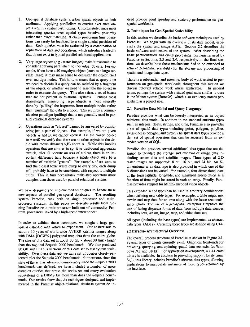
The overall process structure of Paradise is shown in Figure 2.1. Several types of clients currently exist. Graphical front-ends for browsing, querying, and updating spatial data sets exist for Win- dows NT and UNIX. For application development, a C++ class library is available. In addition to providing support for dynamic SQL, this library includes Paradise’s abstract data types, allowing applications to manipulate instances of these types returned by the interface.

337

Figure 2.1 Paradise Process Structure.

The Paradise database system consists of one Query Coordinator (QC) process and one or more Data Server (DS) processes. The QC and DS processes communicate via a communication infra- structure that automatically selects the most efficient transport mechanism. When a message is between processes that do not share a common memory system, a transport protocol like TCP or MPI is used. However, when the communication is between processors on an SMP, memory is used as the transport vehicle.

Clients (applications or GUIs) connect to the QC process. After parsing and optimization, the QC controls the parallel execution of the query on the DS processes. Results sets are collected by the QC for delivery back to the client. Special attention is given to the efficient delivery of result tuples containing large objects such as images. In particular, such attributes are not returned until they are actually used by the application program (typically by invoking a method on the attribute). In addition, only the portion of the object actually needed by the client is retrieved from the relevant DS. Thus, if the attribute is a large multidi- mensional array and client needs only a small subarray out of the middle of the array, only the subarray itself is fetched. However, if the client needs a large portion or the entire attribute, the QC establishes a data pipeline from the DS through the QC to the application so that data can be transferred efficiently and with minimal delay.

The QC and DS are implemented as multithreaded processes on top of the SHORE Storage Manager [Care94]. The SHORE Stor- age Manager provides storage volumes, files of untyped objects, B+-trees, and R*-trees [BeckgO, Gutm84]. Objects can be arbi- trarily large, up to the size of a storage volume. Allocation of space inside a storage volume is performed in terms of fixed-size extents. ARIES [Moha92] is used as SHORE’s recovery mechanism. Locking can be done at multiple granularities (e.g. object, page, or file) with optional lock escalation. Because I/O in UNIX is blocking, SHORE uses a separate I/O process for each mounted storage volume. The I/O processes and the main SHORE server process share the SHORE buffer pool which is kept in shared memory. [Yu96] describes an extension of SHORE and Paradise to handle tape-based storage volumes.

2.3 Basic Parallelism Mechanisms

Paradise uses many of the basic parallelism mechanisms first developed as part of the Gamma project [DeWi90, DeWi921. Tables are fully partitioned across all disks in the system using

round-robin, hash, or spatial declustering (to be discussed below). When a scan or selection query is executed, a separate thread is started for each fragment of each table.

Paradise uses a push model of parallelism to implement partitioned execution [DeWi92] in which tuples are pushed from leaves of the operator tree upward. Every Paradise operator (e.g. join, sort, select, . ..) takes its input from an input stream and places its result tuples on an output stream. Streams are similar in concept to Volcano’s exchange operator [Grae90] except that they are not active entities. Streams themselves are C++ objects and can be specialized in the form of “file streams” and “network streams”. File streams are used to read/write tuples from/to disk. Network streams are used to move data between operators either through shared-memory or across a communications network via a transport protocol (e.g. TCP/IP or MPI). In addition to providing transparent communication between operators on the same or different processors, network streams also provide a flow-control mechanism that is used to regulate the execution rates of the different operators in the pipeline. Network streams can be further specialized into split streams which are used to demultiplex an output stream into multiple output streams based on a function being applied to each tuple. Split streams are one of the key mechanisms used to parallelize queries [DeWi92]. Since all types of streams are derived from a base stream class, their interfaces are identical and the implementation of each operator can be totally isolated from the type of stream it reads or writes. At runtime, the scheduler thread (running in the QC process), which is used to control the parallel execution of the query, instantiates the correct type of stream objects to connect the operators.

2.4 Relational Algorithms

For the most part, Paradise uses relatively standard algorithms for each of the basic relational operators. Indexed selections are provided for both non-spatial and spatial selections. For join operations, the optimizer can choose from nested loops, indexed nested loops, and dynamic memory Grace hash join [Kits89]. Paradise’s query optimizer (which is written using OPT++ [Kabr96]) will consider replicating small outer tables when an index exists on the join column of the inner table.

Most parallel database systems [Shat95] use a two phase approach to the parallel execution of aggregate operations. For example, consider a query involving an average operator with a group by clause. During the first phase each participating thread processes its fragment of the input table producing a running sum and count for each group. During the second phase a single processor (typically) combines the results from the first phase to produce an average value for each group.

Since standard SQL has a well defined set of aggregate operators, for each operator the functions that must be performed during the first and second phases are known when the system is being built and, hence, can be hard coded into the system. However, in the case of an object-relational system that supports type extensibil- ity, the set of aggregate operators is not known in advance as each new type added to the system may introduce new operators. For example, a point ADT might contain a “closest” method which finds the spatially closest polyline.. Like the min aggregate, “closest” must examine a number (possible large) of polylines before finding the correct result.

338

Our solution to this problem is to define all aggregate operators in terms of local and global functions. The local function is executed during the first phase and the global function during the second phase. Each function has a signature in terms of its input and output types. When the system is extended either by adding new ADTS and/or new aggregate operators, the aggregate name along with its local and global functions are registered in the system catalogs. This permits new aggregates to be added without modifying the scheduler or execution engine. A similar approach is used in Illustra/Informix.

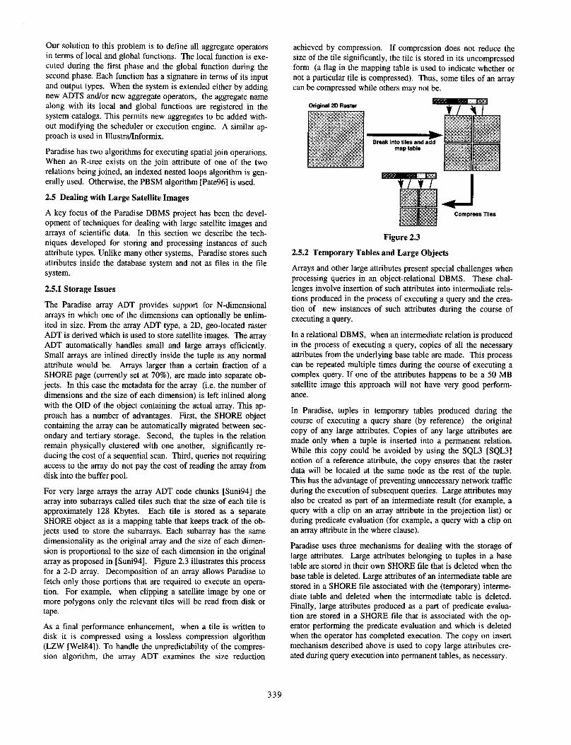
achieved by compression. If compression does not reduce the size of the tile significantly, the tile is stored in its uncompressed form (a flag in the mapping table is used to indicate whether or not a particular tile is compressed). Thus, some tiles of an array can be compressed while others may not be.

Original 2D Raster

Paradise has two algorithms for executing spatial join operations. When an R-tree exists on the join attribute of one of the two relations being joined, an indexed nested loops algorithm is generally used. Otherwise, the PBSM algorithm [Pate961 is used.

2.5 Dealing with Large Satellite Images

A key focus of the Paradise DBMS project has been the development of techniques for dealing with large satellite images and arrays of scientific data. In this section we describe the techniques developed for storing and processing instances of such attribute types. Unlike many other systems, Paradise stores such attributes inside the database system and not as files in the file system.

2.51 Storage Issues

Figure 2.3

2.5.2 Temporary Tables and Large Objects

Arrays and other large attributes present special challenges when processing queries in an object-relational DBMS. These challenges involve insertion of such attributes into intermediate relations produced in the process of executing a query and the creation of new instances of such attributes during the course of executing a query.

The Paradise array ADT provides support for N-dimensional arrays in which one of the dimensions can optionally be unlim- ited in size. From the array ADT type, a 2D, geo-located raster ADT is derived which is used to store satellite images. The array ADT automatically handles small and large arrays efficiently. Small arrays are inlined directly inside the tuple as any normal attribute would be. Arrays larger than a certain fraction of a SHORE page (currently set at 70%), are made into separate objects. In this case the metadata for the array (i.e. the number of dimensions and the size of each dimension) is left inlined along with the OID of the object containing the actual array. This approach has a number of advantages. First, the SHORE object containing the array can be automatically migrated between secondary and tertiary storage. Second, the tuples in the relation remain physically clustered with one another, significantly reducing the cost of a sequential scan. Third, queries not requiring access to the array do not pay the cost of reading the array from disk into the buffer pool.

In a relational DBMS, when an intermediate relation is produced in the process of executing a query, copies of all the necessary attributes from the underlying base table are made. This process can be repeated multiple times during the course of executing a complex query. If one of the attributes happens to be a 50 MB satellite image this approach will not have very good performance.

In Paradise, tuples in temporary tables produced during the course of executing a query share (by reference) the original copy of any large attributes. Copies of any large attributes are made only when a tuple is inserted into a permanent relation. While this copy could be avoided by using the SQL3 [SQL31 notion of a reference attribute, the copy ensures that the raster data will be located at the same node as the rest of the tuple. This has the advantage of preventing unnecessary network traffic

For very large arrays the array ADT code chunks [Suni94] the during the execution of subsequent queries. Large attributes may array into subarrays called tiles such that the size of each tile is also be created as part of an intermediate result (for example, a approximately 128 Kbytes. Each tile is stored as a separate query with a clip on an array attribute in the projection list) or SHORE object as is a mapping table that keeps track of the ob- during predicate evaluation (for example, a query with a clip on jects used to store the subarrays. Each subarray has the same an array attribute in the where clause). dimensionality as the original array and the size of each dimension is proportional to the size of each dimension in the original array as proposed in [Suni94]. Figure 2.3 illustrates this process for a 2-D array. Decomposition of an array allows Paradise to fetch only those portions that are required to execute an operation. For example, when clipping a satellite image by one or more polygons only the relevant tiles will be read from disk or tape.

As a final performance enhancement, when a tile is written to disk it is compressed using a lossless compression algorithm (LZW [We184]). To handle the unpredictability of the compression algorithm, the array ADT examines the size reduction

Paradise uses three mechanisms for dealing with the storage of large attributes. Large attributes belonging to tuples in a base table are stored in their own SHORE tile that is deleted when the base table is deleted. Large attributes of an intermediate table are stored in a SHORE tile associated with the (temporary) intermediate table and deleted when the intermediate table is deleted. Finally, large attributes produced as a part of predicate evaluation are stored in a SHORE file that is associated with the operator performing the predicate evaluation and which is deleted when the operator has completed execution. The copy on insert mechanism described above is used to copy large attributes created during query execution into permanent tables, as necessary.

339

2.52 The Need for Pull

As discussed in Section 2.3, Paradise use a push model of parallelism. Unfortunately, the push model of parallelism breaks down when dealing with large attributes such as satellite images. In particular, in the process of executing a query involving the redistribution of intermediate tuples between processors one does not want to unnecessarily copy large attributes.

Paradise uses two tactics to deal with this problem. First, whenever possible, the optimizer avoids declustering tuples containing large attributes. When this is not possible, Paradise turns to using a pull model of parallelism. Consider a query involving the clip of a set of raster images by a set of polygons corresponding to selected areas of interest (e.g. wetlands). Assume that the two relations are not spatially partitioned on the same grid so that the tuples of one of the two relations must be redeclustered in order to process the query. Assume further that the optimizer decides that it is less expensive to redecluster the tuples “containing” the raster images. One approach would be to push both the tuples and their associated images. While this approach would produce the correct result, more data than is actually needed to process the query will be moved between processors.

Instead, Paradise uses a pull model in this situation. In particular, when the clip0 method is invoked on an instance of the array ADT, if the array is not stored on same node as the node on which the clip is being performed, the array ADT starts an operator on the node on which the array is stored to fetch only those tiles containing portions of the array covered by the clip0

Pull is also used when a redistributed tuple is inserted into a permanent result relation. As discussed in the previous section, a copy of any large attributes are made in this case. Using pull insures that only the required data is actually moved between processors.

In general, pull is an expensive operation because each pull requires that a separate operator be started on the remote node. In addition, the pull operator results in extra random disk seeks. While we were aware of these costs we were not able to architect a good solution that totally avoided the use of pull and, in the end, concluded that overhead of the pull was acceptable relative to the size of the objects being pulled.

2.6 Declustering Arrays - Good or Bad?

A fundamental question with respect to the parallelization of operations in Paradise is whether the tiles of a single large image should be declustered across multiple disks. This is relatively easy to do in Paradise. First, the Paradise array ADT already decomposes large arrays into multiple tiles. Second, as discussed in the previous section, the array ADT knows how to pull pieces of an array residing on a disk attached to a different processor.

Just as partitioning the tuples of a table facilitates parallelization of relational operations, partitioning a large image across multiple disks facilitates the parallel application of a function to the entire image (e.g. searching the image for Scud missile launchers or clipping the image by a set of polygons). While partitioning a table is almost always beneficial (except for very small tables), the same is not true for arrays. For example, clipping many images by a few polygons or searching a large collection of photos for ones that contain red sunsets provides almost no benefit as long as the number of images to be processed is much larger than

the number of processors. However, computing the pixel-by- pixel average of a few arrays would benefit from declustering each of the arrays.

There seems to be no right answer. It may be best to store the tiles from each image on one or two disks on the same processor and then repartition “on the fly” when a query involves a com- putationally intensive operation on only a few images. This approach has the added benefit of simplifying the task of migrating images between secondary and tertiary storage. In Section 3 we experimentally explore the tradeoffs associated with partitioning images.

2.7 Spatial Query Parallelization

2.7.1 Spatial Declustering

In addition to hash and round-robin partitioning, Paradise can also spatially decluster the tuples in a table. The basic idea of spatial declustering is to divide the spatial domain into multiple 2-D partitions which are, in turn, mapped to storage units either by hashing or in a round-robin fashion. As a spatially declustered table is being loaded, a spatial attribute of each tuple is used to determine which partition the tuple belongs to. The same spatial partitioning scheme can be used for multiple tables in order to maximize the amount of “local” processing for queries involving spatial join operations between the two tables. In addition to point, poIyline, and polygon data, one can also spatially decluster geo-located image data such as satellite images or oil field seis- mic data.

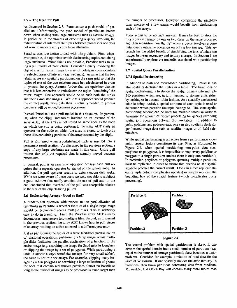
While spatial declustering is attractive from a performance view- point, several factors complicate its use. First, as illustrated by Figure 2.4, when spatial partitioning non-point data (i.e., polylines or polygons), it is impossible to map every polyline or polygon to a single partition (unless there is only one partition!). In particular, polylines or polygons spanning multiple partitions must be replicated in order to insure that queries on the spatial attribute produce the correct result. One can either replicate the entire tuple (which complicates updates) or simply replicate the bounding box of the spatial feature (which complicates query processing).

Figure 2.4

The second problem with spatial partitioning is skew. If one divides the spatial domain into a small number of partitions (e.g. equal to the number of storage partitions), skew becomes a major problem. Consider, for example, a relation of road data for the State of Wisconsin. If one spatially divides the state into say 16 partitions, then those partitions containing data from Madison, Milwaukee, and Green Bay will contain many more tuples than

340

the partition corresponding to the area around Rhinelander (which is in north-central Wisconsin). Likewise, partitions containing large areas of Lake Michigan or Lake Superior will have relatively few tuples mapped to them.

As proposed in [Huagl, DeWi92b], one way to reduce the effects of partition skew [Walt911 is to significantly increase the number of partitions being used. Unfortunately, increasing the number of partitions, increases the number of tuples spanning multiple partitions and, hence, the percentage of tuples that must be replicated. Our preliminary tests showed that one needs thousands of partitions to smooth out the skew to any significant extent. An alternative approach to dealing with skew is to decluster based upon the distribution of the data set. Koudas et al. [Koud96] describe an interesting approach based upon declustering the leaves of an R-tree. One difficulty with such an approach is that it makes the parallelization of queries of multiple data sets less efficient, since the multiple data sets will not be declustered on the same boundaries.

2.7.2 Parallel Spatial Join Processing

Like a normal join operation, execution of a spatial join query in parallel is a two phase process. During the first phase, tuples of the two relations to be joined are redeclustered on their join attributes in order to bring candidate tuples together. For non- spatial attributes this is normally done by hashing the join attribute values to map each attribute value to a processor. In the second phase, each of the participating processors joins the two partitions of tuples it receives during the first phase. Any single processor spatial join algorithm (e.g. PBSM [Pate96]) can be used during this second phase. If either of the input tables are already declustered on their joining attributes, then the first phase of the algorithm can be eliminated for that table.

For joins on spatial attributes the process is slightly more com- plicated, First, the partitioning function must be a spatial partitioning function mapping tuples to partitions of a 2-D space (see Section 2.7.1). Second, in order to minimize the effects of spatial skew during the second phase of the algorithm, many more partitions than processors must be used. Third, since the spatial attributes of some tuples will span multiple spatial partitions, replication must be used during the repartitioning phase to insure that the correct result is produced. Finally, replicating tuples introduces the possibility that duplicate tuples will be produced. Consider, for example, tables of river and road data for Wiscon- sin and a query to determine whether the Wisconsin river and U.S. 90 cross each other. Both the Wisconsin river and U.S. 90 span multiple spatial partitions and it turns out that they cross each other in two places. In the process of redeclustering the river and road data during phase one, both objects will get replicated once for each partition they overlap. If the two partitions where they cross get mapped to different processors, then the result of the query will contain two identical result tuples.

We have also designed and implemented other parallel spatial join algorithms involving the replication of only bounding box information and not full tuples. A description and analysis of the performance of these algorithms can be found in [Pate97].

2.7.3 Spatial Aggregation Processing

A geo-spatial database system opens up an entire new spectrum of operations that cannot be handled efficiently by normal relational query processing techniques. Consider, for example a

341

query to find the river closest to a particular point. To process this operation one must iteratively expand a circle around the point until the circle overlaps the polyline corresponding to some river. Since an expansion step may find more than one candidate river, all but the closest must be eliminated. We consider this type of operation to be a form of “spatial aggregate” query as it not totally dissimilar to the task of executing a SQL min operation.

This type of operation can be extended to include what we term a “spatial join with aggregation” query. Consider the query to find the closest river to cities with populations greater than one million. First the selection predicate is applied to the Cities table to filter out all cities with populations less than one million. The remaining cities must then be “joined” with the Rivers table. But the notion of join in this case is not overlap but rather a spatial aggregate function which defines join satistiability as spatially closest.

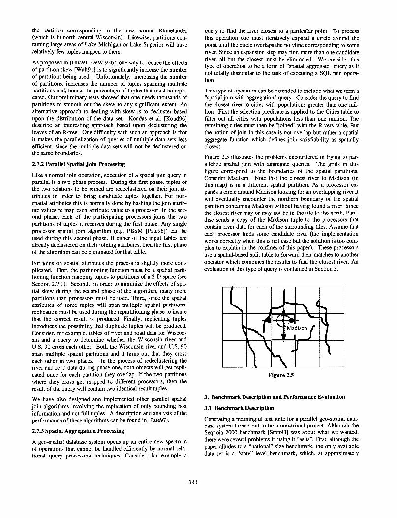
Figure 2.5 illustrates the problems encountered in trying to parallelize spatial join with aggregate queries. The grids in this figure correspond to the boundaries of the spatial partitions. Consider Madison. Note that the closest river to Madison (in this map) is in a different spatial partition. As a processor expands a circle around Madison looking for an overlapping river it will eventually encounter the northern boundary of the spatial partition containing Madison without having found a river. Since the closest river may or may not be in the tile to the north, Para- dise sends a copy of the Madison tuple to the processors that contain river data for each of the surrounding tiles. Assume that each processor finds some candidate river (the implementation works correctly when this is not case but the solution is too complex to explain in the confines of this paper). These processors use a spatial-based split table to forward their matches to another operator which combines the results to find the closest river. An evaluation of this type of query is contained in Section 3.

Figure 2.5

3. Benchmark Description and Performance Evaluation

3.1 Benchmark Description

Generating a meaningful test suite for a parallel geo-spatial database system turned out to be a non-trivial project. Although the Sequoia 2000 benchmark [Ston93] was about what we wanted, there were several problems in using it “as is”. First, although the paper alludes to a “national” size benchmark, the only available data set is a “state” level benchmark, which, at approximately

lGB, was far too small to use for testing scaleup or speedup. Second, the spatial queries in the benchmark are relatively sim- ple. Third, the original Sequoia benchmark provided no mechanism for scaling the database. We address each of these issues in turn.

3.1.1 A Global Sequoia Data Set

Following the Sequoia lead of using “real” data for the benchmark, we used 10 years of 8 Km. resolution AVHRR satellite images obtained from NASA for our raster images. Each raster is a composite image covering the entire world. For polygon data, we used a DCW [DCW92] global data set containing a variety of information about such things as roads, cities, land use, and drainage properties. Both data sets were geo-registered to the same coordinate system. The definition of the five tables used is given below. raster ( date Date,

channel Integer, // recording channel data Raster16); N raster image

populatedPlaces ( id String, II unique feature identifier containingface String, /I feature-id of containing polygon type Integer, N category of populated place (6 values) location Point, N spatial coordinates of the place name String); // name of the place

landcover (id String, /I unique feature identifier type Integer, // type of the water-body (16 categories) shape Polygon); It boundary of the water body

roads (id String, II unique feature identifier type Integer, //type of road (8 possible categories) shape Polyline); /I shape of the road

drainage (id String, /I unique feature identifier type Integer, // drainage feature type (21 categories) shape Polyline); N shape of the drainage feature

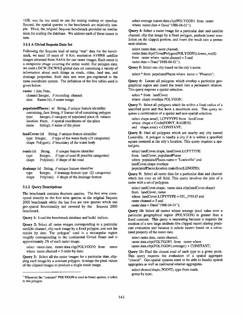
3.1.2 Query Descriptions

The benchmark contains fourteen queries. The first nine correspond directly to the first nine queries in the original Sequoia 2000 benchmark while the last five are new queries which test geo-spatial functionality not covered by the Sequoia 2000 benchmark.

Query 1: Load the benchmark database and build indices.

Query 2: Select all raster images corresponding to a particular satellite channel, clip each image by a fixed polygon, and sort the results by date. The polygon’ used is a rectangular region roughly corresponding to the continental United States and is approximately 2% of each raster image.

select raster.date, raster.data.clip(POLYGON) from raster where raster.channel= 5 order by date;

Query 3: Select all the raster images for a particular date, clipping each image by a constant polygon. Average the pixel values of the clipped images to produce a single result image.

’ Whenever the “constant” POLYGON is used in future queries, it refers to this polygon.

select average (raster.data.clip(POLYGON) from raster where raster.date = Date(“1988-04-01”);

Query 4: Select a raster image for a particular date and satellite channel, clip that image by a fixed polygon, perform lower resolution on the clipped portion, and insert the result into a permanent relation.

select raster.date, raster.channel, raster.data.clip(ClosedPolygon(POLYGON)).lower_res(8) from raster where raster.channel = 5 and raster.date = Date(“1988-04-01”);

Query 5: Select one city based on the city’s name.

select * from populatedPlaces where name = “Phoenix”;

Query 6: Locate all polygons which overlap a particular geographical region and insert the result into a permanent relation. This query requires a spatial selection.

select * from landcover where shape overlaps POLYGON;

Query 7: Select all polygons which lie within a fixed radius of a specified point and that have a maximum area. This query requires a combination of a spatial and non-spatial selection.

select shape.area(), LCPYTYPE from landcover where shape < Circle(POINT, RADIUS) and shape.area() < CONSTANT;

Query 8: Find all polygons which are nearby any city named Louisville. A polygon is nearby a city if it is within a specified square centered at the city’s location. This query requires a spatial join.

select landcovershape, landCover.LCPYTYPE from landcover, populatedPlaces where populatedPlaces.name = “Louisville” and landCover.shape overlaps populatedPlaces.location.makeBox(LENGTH);

Query 9: Select all raster data for a particular date and channel which lies over an oil field. This query involves the join of a raster with a set of polygons.

select landCover.shape, raster.data.clip(landCover.shape) from landcover, raster where landCover.LCPYTYPE = OIL-FIELD and raster.channel = 5 and raster.date = Date(“1988-04-01”);

Query 10: Select all rasters whose average pixel value over a particular geographical region (POLYGON) is greater than a fixed constant. This query is interesting because it requires the creation of a new large attribute (the clipped raster) during predicate evaluation and because it selects rasters based on a calcu- lated property of the raster data.

select raster.date, raster.channel, raster.data.clip(POLYGON) from raster where raster.data.clip(POLYGON).average() > CONSTANT;

Query 11: Find the closest road of each type to a given point. This query requires the evaluation of a spatial aggregate “closest”. Geo-spatial systems need to be able to handle spatial aggregates as well as traditional relation aggregates.

select closest(shape, POINT), type from roads group by type;

342

Query 12: Find the closest drainage feature (i.e. lake, river) to every large city. This query requires the evaluation of a spatial aggregate on a cross product of two relations. To make this query work efficiently in parallel, a system must have spatial declustering and must support spatial semi-join.

select closest(drainage.shape, populatedPlaces.location), populatedPlaces.location from drainage, populatedPlaces where populatedPlaces.location overlaps drainage.shape and populatedPlaces.type = LARGE-CITY group by populatedPlaces.location

This query demonstrates one of the novel techniques that Para- dise uses for handling geo-spatial data. Since we have not described this approach elsewhere, we digress for a moment to describe the approach here. This query is executed as follows:

1. Declustering the drainage relation: The spatial region in which all the drainage features lie (the “universe2” of the shape attribute) is broken up into 10,000 tiles. The tiles are then numbered in a row-major order starting at the upper- left comer. Each tile is mapped to one of the nodes by hashing on tile number. The drainage relation is then spatially declustered by sending each tuple to the node corresponding to the tile in which its shape attribute is located. Drainage features that span tiles mapped to multiple nodes are replicated at all the corresponding nodes.

2. Declustering the points relation: The points are spatially declustered using the same declustering policy used in the previous step.

3. A spatial index on the shape attribute of the declustered drainage relation is built on the fly. (The index is local to each node, and is built only on the fragment of the drainage relation at that node).

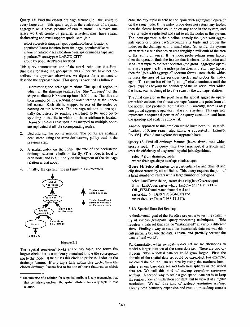
4. Finally, the operator tree in Figure 3.1 is executed.

Index Scan on Drainage

4 4

Tuples cross node boundary

Tuples transferred between operators on the same node

scan city

Figure 3.1

The “spatial semi-join” looks at the city tuple, and forms the largest circle that is completely contained in the tile corresponding to that node. It then uses this circle to probe the index on the drainage feature. If any tuple falls within this circle, then the closest drainage feature has to be one of these features, in which

* The universe of a relation for a spatial attribute is any rectangular box that completely encloses the spatial attribute for every tuple in that relation.

case, the city tuple is sent to the “join with aggregate” operator on the same node. If the index probe does not return any tuples, then the closest feature could be on any node in the system, and the city tuple is replicated and sent to all the nodes in the system. The next operator in the pipeline, namely the “join with aggregate operator”, takes each incoming city tuple and probes the index on the drainage with a small circle (currently, the system starts with a circle that has an area roughly a millionth of the area of the entire universe). If the index probe returns some tuples, then the operator finds the feature that is closest to the point and sends that tuple to the next operator (the global aggregate operator) in the pipeline. If the index probe does not return any tuples, then the “join with aggregate” operator forms a new circle, which is twice the area of the previous circle, and probes the index again. This expansion of the “probing” circle continues until the circle expands beyond the boundary of the universe, after which the index scan is changed to a file scan on the drainage relation.

The final operator in the pipeline is the global aggregate operator, which collects the closest drainage feature to a point from all the nodes, and produces the final result. Currently, there is only one global aggregate operator in the entire system. This operator represents a sequential portion of the query execution, and hurts the speedup and scaleup somewhat.

Another approach to this problem would have been to use modi- fications of R-tree search algorithms, as suggested in IKim96, Rous951. We did not explore that approach here.

Query 13: Find all drainage features (lakes, rivers, etc.) which cross a road. This query joins two large spatial relations and tests the efficiency of a system’s spatial join algorithms.

select * from drainage, roads where drainageshape overlaps roads.shape;

Query 14: Select all rasters for a particular year and channel and clip those rasters by all oil fields. This query requires the join of a large number of rasters with a large number of polygons.

select landCover.shape, raster.data.clip(landCover.shape) from landcover, raster where landCover.LCPYTYPE = OIL-FIELD and raster.channel = 5 and raster.date >= Date(“1988-04-01”) and raster.date <= Date(“1988-12-31”);

3.1.3 Spatial Data Set Scaleup

A fundamental goal of the Paradise project is to test the scalability of various geo-spatial query processing techniques. This requires a data set that can be “instantiated” at various different sizes. Finding a way to scale our benchmark data set was difti- cult partially because the data is spatial and partially because the data is “real world”.

Fundamentally, when we scale a data set we are attempting to model a larger instance of the same data set. There are two or- thogonal ways a spatial data set could grow larger. First, the domain of the spatial data set could be expanded. For example, we could double the data set size by using the northern hemi- sphere as our base data set and both hemispheres as the scaled data set. We call this kind of scaleup boundary expansion scaleup. A second way to scale a geo-spatial data set is to keep the region under consideration constant, but to view it at a higher resolution. We call this kind of scaleup resolution scaleup. Clearly both boundary expansion and resolution scaleup cause a

343

data set to grow, and both are of interest. For our experiments, we chose to use resolution scaleup. We considered a number of approaches for simulating resolution scaleup on a fixed- resolution real-world data set, and settled on the following.

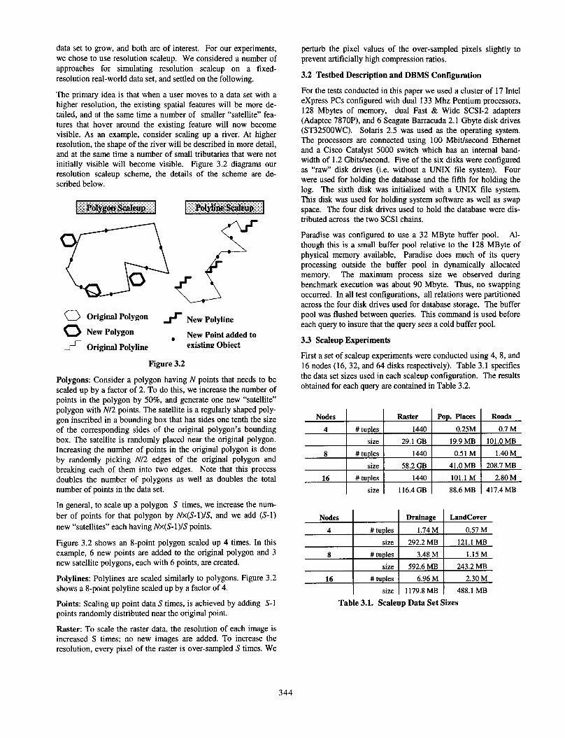
The primary idea is that when a user moves to a data set with a higher resolution, the existing spatial features will be more de- tailed, and at the same time a number of smaller “satellite” features that hover around the existing feature will now become visible. As an example, consider scaling up a river. At higher resolution, the shape of the river will be described in more detail, and at the same time a number of small tributaries that were not initially visible will become visible. Figure 3.2 diagrams our resolution scaleup scheme, the details of the scheme are described below.

i-

a @-kinal Pobwn x New polyline

0 New Polygon New Point added to -5 Original Polyline

, existing Obiect

Figure 3.2

Polygons: Consider a polygon having N points that needs to be scaled up by a factor of 2. To do this, we increase the number of points in the polygon by 50%, and generate one new “satellite” polygon with N/2 points. The satellite is a regularly shaped polygon inscribed in a bounding box that has sides one tenth the size of the corresponding sides of the original polygon’s bounding box. The satellite is randomly placed near the original polygon. Increasing the number of points in the original polygon is done by randomly picking N/2 edges of the original polygon and breaking each of them into two edges. Note that this process doubles the number of polygons as well as doubles the total number of points in the data set.

In general, to scale up a polygon S times, we increase the number of points for that polygon by Nx(S-1)/S, and we add (S-l) new “satellites” each having Nx(41)IS points.

Figure 3.2 shows an 8-point polygon scaled up 4 times. In this example, 6 new points are added to the original polygon and 3 new satellite polygons, each with 6 points, are created.

Polylines: Polylines are scaled similarly to polygons. Figure 3.2 shows a 8-point polyline scaled up by a factor of 4.

Points: Scaling up point data S times, is achieved by adding S-l points randomly distributed near the original point.

Raster: To scale the raster data, the resolution of each image is increased S times; no new images are added. To increase the resolution, every pixel of the raster is over-sampled S times. We

perturb the pixel values of the over-sampled pixels slightly to prevent artificially high compression ratios.

3.2 Testbed Description and DBMS Configuration

For the tests conducted in this paper we used a cluster of 17 Intel express PCs configured with dual 133 Mhz Pentium processors, 128 Mbytes of memory, dual Fast L?z Wide SCSI-2 adapters (Adaptec 787OP), and 6 Seagate Barracuda 2.1 Gbyte disk drives (ST325OOWC). Solaris 2.5 was used as the operating system. The processors are connected using 100 Mbit/second Ethernet and a Cisco Catalyst 5000 switch which has an internal band- width of 1.2 Gbits/second. Five of the six disks were configured as “raw” disk drives (i.e. without a UNIX tile system). Four were used for holding the database and the fifth for holding the log. The sixth disk was initialized with a UNIX file system. This disk was used for holding system software as well as swap space. The four disk drives used to hold the database were distributed across the two SCSI chains.

Paradise was configured to use a 32 MByte buffer pool. Al- though this is a small buffer pool relative to the 128 MByte of physical memory available, Paradise does much of its query processing outside the buffer pool in dynamically allocated memory. The maximum process size we observed during benchmark execution was about 90 Mbyte. Thus, no swapping occurred. In all test configurations, all relations were partitioned across the four disk drives used for database storage. The buffer pool was flushed between queries. This command is used before each query to insure that the query sees a cold buffer pool.

3.3 Scaleup Experiments

First a set of scaleup experiments were conducted using 4, 8, and 16 nodes (16,32, and 64 disks respectively). Table 3.1 specifies the data set sizes used in each scaleup configuration. The results obtained for each query are contained in Table 3.2.

Nodes 4

8

16

Raster Pop. Places Roads # tuples 1440 0.25M 0.7 M

size 29.1 GB 19.9 MB 101.0 MB # tuples 1440 0.51 M 1.40 M

size 58.2 GB 41 .O MB 208.7 MB # tuples 1440 101.1 M 2.80 M

size 116.4 GB 88.6 MB 417.4 MB

Nodes Drainage LandCover 4 # tuples 1.74M 0.57 M

size 292.2 MB 121.1 MB 8 # tuples 3.48 M 1.15 M

size 592.6 MB 243.2 MB 16 # tuples 6.96 M 2.30 M

size 1179.8 MB 488.1 MB Table 3.1. Scaleup Data Set Sizes

344

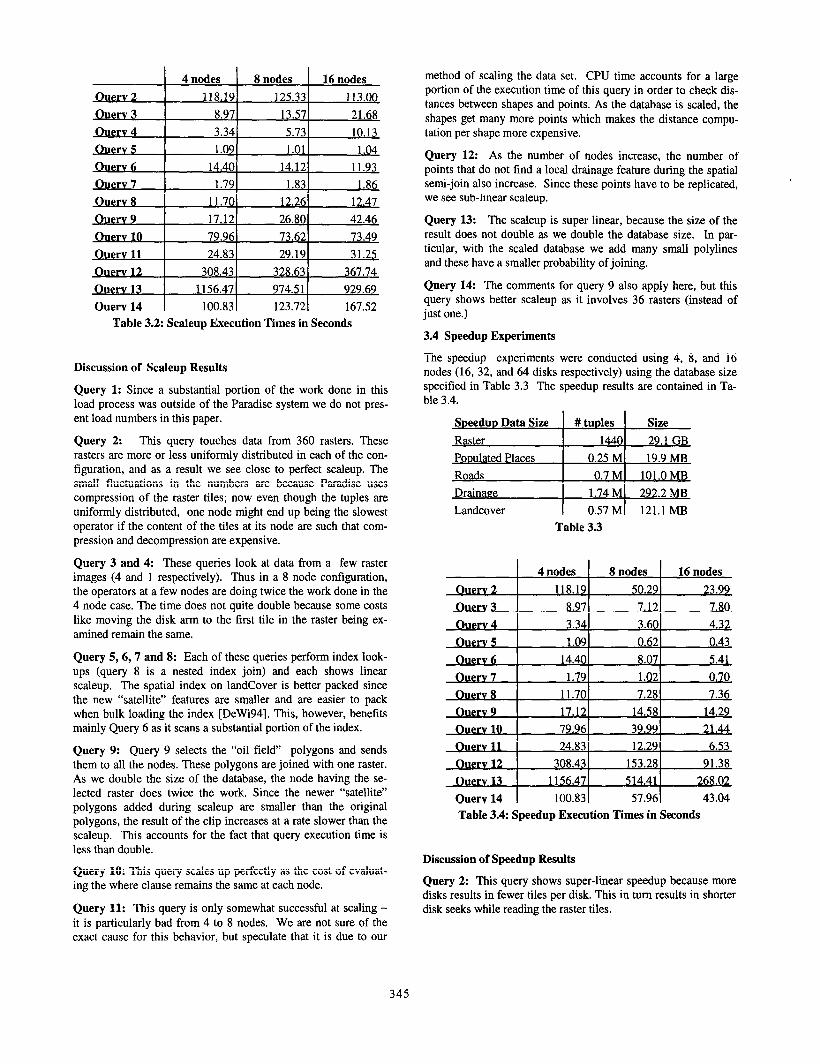
Table 3.2: Scaleup Execution Times in Seconds

Discussion of Scaleup Results

Query 1: Since a substantial portion of the work done in this load process was outside of the Paradise system we do not present load numbers in this paper.

Query 2: This query touches data from 360 rasters. These rasters are more or less uniformly distributed in each of the configuration, and as a result we see close to perfect scaleup. The small fluctuations in the numbers are because Paradise uses compression of the raster tiles; now even though the tuples are uniformly distributed, one node might end up being the slowest operator if the content of the tiles at its node are such that compression and decompression are expensive.

Query 3 and 4: These queries look at data from a few raster images (4 and 1 respectively). Thus in a 8 node configuration, the operators at a few nodes are doing twice the work done in the 4 node case. The time does not quite double because some costs like moving the disk arm to the first tile in the raster being ex- amined remain the same.

Query 5,6,7 and 8: Each of these queries perform index lookups (query 8 is a nested index join) and each shows linear scaleup. The spatial index on landCover is better packed since the new “satellite” features are smaller and are easier to pack when bulk loading the index [DeWi94]. This, however, benefits mainly Query 6 as it scans a substantial portion of the index.

Query 9: Query 9 selects the “oil field” polygons and sends them to all the nodes. These polygons are joined with one raster. As we double the size of the database, the node having the selected raster does twice the work. Since the newer “satellite” polygons added during scaleup are smaller than the original polygons, the result of the clip increases at a rate slower than the scaleup. This accounts for the fact that query execution time is less than double.

Query 10: This query scales up perfectly as the cost of evaluat- ing the where clause remains the same at each node.

Query 11: This query is only somewhat successful at scaling - it is particularly bad from 4 to 8 nodes. We are not sure of the exact cause for this behavior, but speculate that it is due to our

method of scaling the data set. CPU time accounts for a large portion of the execution time of this query in order to check dis- tances between shapes and points. As the database is scaled, the shapes get many more points which makes the distance computation per shape more expensive.

Query 12: As the number of nodes increase, the number of points that do not find a local drainage feature during the spatial semi-join also increase. Since these points have to be replicated, we see sub-linear scaleup.

Query 13: The scaleup is super linear, because the size of the result does not double as we double the database size. In particular, with the scaled database we add many small polylines and these have a smaller probability of joining.

Query 14: The comments for query 9 also apply here, but this query shows better scaleup as it involves 36 rasters (instead of just one.)

3.4 Speedup Experiments

The speedup experiments were conducted using 4, 8, and 16 nodes (16, 32, and 64 disks respectively) using the database size specified in Table 3.3 The speedup results are contained in Ta- ble 3.4.

Speedup Data Size # tuples Size Raster 1440 29.1 GB Ponulated Places 0.25 M 19.9 MB Roads 0.7 M 101.0 MB Drainage 1.74 M 292.2 MB Landcover 0.57 M 121.1 MB

Table 3.3

Ouerv 11 24.83 12.29 6.53 Ouerv 12 308.43 153.28 91.38

268.02 1156.47 514.41 Ouerv 14 100.83 57.96 43.04 Table 3.4: Speedup Execution Times in Seconds

Discussion of Speedup Results

Query 2: This query shows super-linear speedup because more disks results in fewer tiles per disk. This in turn results in shorter disk seeks while reading the raster tiles.

345

Query 3 and 4: These queries look at data from only a few raster images (4 and 1 respectively). Since the individual raster images reside on single disks, these queries do not exhibit speedup.

Query 5, 6, 7 and 8: These queries involve index lookups (query 8 is a index nested loops spatial join). As the data is spread among more nodes, the indices become smaller at each node. The speedup is less than linear because the index size de- creases at a logarithmic rate.

Query 9: There is no parallelism in this query, since it involves only a single raster, and all the processing for the query is done at the node that holds the selected raster.

Query 10: Most of the work involved in this query lies in evalu- ating the predicate in the “where” clause. Since this work is evenly distributed, we see good speedup.

Query 11 and 12: The local aggregation at each node benefits from increasing the degree of parallelism. However, as we discussed in the scaleup section, the global aggregate evaluation remains sequential, reducing speedup slightly below linear.

Query 13: The PBSM spatial join algorithm, just like relational hash join algorithms, forms partitions that are joined. When increasing the nodes from 4 to 8 all the partitions fit in memory, resulting in super-linear speedup

Query 14: The performance of this query is similar to that of query 9, but here we see better speedup because more rasters are selected.

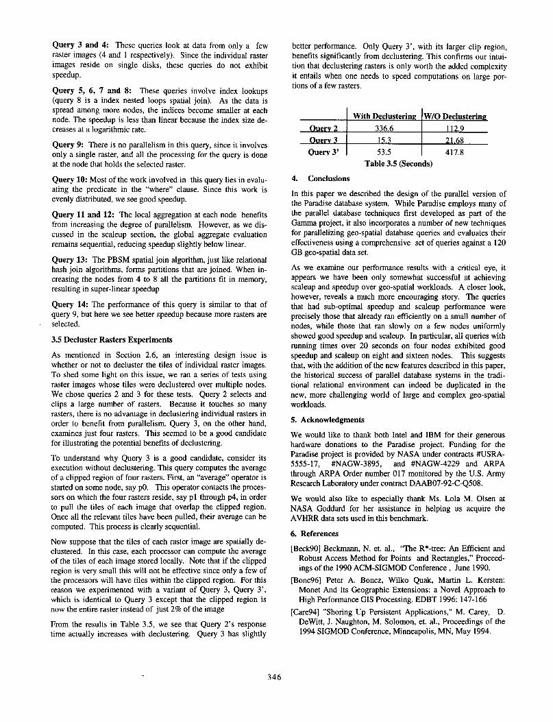
3.5 Decluster Rasters Experiments

As mentioned in Section 2.6, an interesting design issue is whether or not to decluster the tiles of individual raster images. To shed some light on this issue, we ran a series of tests using raster images whose tiles were declustered over multiple nodes. We chose queries 2 and 3 for these tests. Query 2 selects and clips a large number of rasters. Because it touches so many rasters, there is no advantage in declustering individual rasters in order to benefit from parallelism. Query 3, on the other hand, examines just four rasters. This seemed to be a good candidate for illustrating the potential benefits of declustering.

To understand why Query 3 is a good candidate, consider its execution without declustering. This query computes the average of a clipped region of four rasters. First, an “average” operator is started on some node, say p0. This operator contacts the processors on which the four rasters reside, say pl through p4, in order to pull the tiles of each image that overlap the clipped region. Once all the relevant tiles have been pulled, their average can be computed. This process is clearly sequential.

Now suppose that the tiles of each raster image are spatially declustered. In this case, each processor can compute the average of the tiles of each image stored locally. Note that if the clipped region is very small this will not be effective since only a few of the processors will have tiles within the clipped region. For this reason we experimented with a variant of Query 3, Query 3’, which is identical to Query 3 except that the clipped region is now the entire raster instead of just 2% of the image

From the results in Table 3.5, we see that Query 2’s response time actually increases with declustering. Query 3 has slightly

better performance. Only Query 3’, with its larger clip region, benefits significantly from declustering. This confirms our intui- tion that declustering rasters is only worth the added complexity it entails when one needs to speed computations on large portions of a few rasters.

With Declustering W/O DeclusterinK 336.6 112.9

Ouerv 3 15.3 21.68 Ouerv 3’ 53.5 417.8

Table 3.5 (Seconds)

4. Conclusions

In this paper we described the design of the parallel version of the Paradise database system. While Paradise employs many of the parallel database techniques first developed as part of the Gamma project, it also incorporates a number of new techniques for parallelizing geo-spatial database queries and evaluates their effectiveness using a comprehensive set of queries against a 120 GB geo-spatial data set.

As we examine our performance results with a critical eye, it appears we have been only somewhat successful at achieving scaleup and speedup over geo-spatial workloads. A closer look, however, reveals a much more encouraging story. The queries that had sub-optimal speedup and scaleup performance were precisely those that already ran efficiently on a small number of nodes, while those that ran slowly on a few nodes uniformly showed good speedup and scaleup. In particular, all queries with running times over 20 seconds on four nodes exhibited good speedup and scaleup on eight and sixteen nodes. This suggests that, with the addition of the new features described in this paper, the historical success of parallel database systems in the traditional relational environment can indeed be duplicated in the new, more challenging world of large and complex geo-spatial workloads.

5. Acknowledgments

We would like to thank both Intel and IBM for their generous hardware donations to the Paradise project. Funding for the Paradise project is provided by NASA under contracts #USRA- 5555-17, #NAGW-3895, and #NAGW-4229 and ARPA through ARPA Order number 017 monitored by the U.S. Army Research Laboratory under contract DAAB07-92-C-Q508.

We would also like to especially thank Ms. Lola M. Olsen at NASA Goddard for her assistance in helping us acquire the AVHRR data sets used in this benchmark.

6. References

[Beck901 Beckmann, N. et. al., “The R*-tree: An Efficient and Robust Access Method for Points and Rectangles,” Proceed- ings of the 1990 ACM-SIGMOD Conference , June 1990.

[Bonc96] Peter A. Boncz, Wilko Quak, Martin L. Kersten: Monet And Its Geographic Extensions: a Novel Approach to High Performance GIS Processing. EDBT 1996: 147- 166

[Care941 “Shoring Up Persistent Applications,” M. Carey, D. Dewitt, J. Naughton, M. Solomon, et. al., Proceedings of the 1994 SIGMOD Conference, Minneapolis, MN, May 1994.

346

[DCW92] VPFView 1.0 Users Manual for the Digital Chart of the World, Defense Mapping Agency, July 1992.

[Dew901 D. Dewitt, et. al., ‘The Gamma Database Machine Project”, IEEE Transactions on Knowledge and Data Engi- neering, March, 1990.

[DeWi92] D. Dewitt and J. Gray, “Parallel Database Systems: The Future of Database Processing or a Passing Fad?,” Communications of the ACM, June, 1992.

[DeWi92] Dewitt, D., Naughton, J., Schneider, D, and S. Se- shadri, “Practical Skew Handling in Parallel Joins,” Proceed- ings of the 1992 Very Large Data Base Conference, Vancou- ver, CA, August 1992.

[DeWi94] Dewitt, D. J., N. Kabra, J. Luo, J. M. Patel, and J. Yu, “Client-Server Paradise”. In Proceedings of the 20th VLDB Conference, September, 1994.

[EOS96] See: http://eos.nasa.gov/ [Grae90] Graefe, G., “Encapsulation of Parallelism in the Vol-

cano Query Processing System,” Proceedings of the 1990 ACM-SIGMOD International Conference on Management of Data, May 1990.

[Gutm84] A. Gutman, “R-trees: A Dynamic Index Structure for Spatial Searching,” Proceedings of the 1984 ACM-SIGMOD Conference, Boston, Mass. June 1984.

[HuBl] Hua, K.A. and C. Lee, “Handling Data Skew in Multi- processor Database Computers Using Partition Tuning,” Pro- ceedings of the 17” VLDB Conference”, Barcelon a, Spain, September, 1991.

[Info961 See http://www.informix.com/ [Illu96] See http://www.illustra.com/ [Moha92] Mohan, C., et. Al., “ARIES: A transaction recovery

methods supporting fine-granularity locking and partial roll- backs using write-ahead logging,” ACM TODS, March 1992.

[Kabr96] Kabra, N. and D. Dewitt, Opt++ - An Object Ori- ented Implementation for Extensible Database Query Optimi- zation, submitted for publication. See also:

http://www.cs.wisc.edu/-navinJresearch/opt++.ps [Kits901 Kitsuregawa, M., Nakayama, M. and M. Takagi, ‘The

Effect of Bucket Size Tuning in the Dynamic Hybrid Grace Hash Join Method,” Proceedings of the 1989 VLDB Confer- ence, Amsterdam, August 1989.

[Koud96] Nick Koudas, Christos Faloutsos, Ibrahim Kamell, “Declustering Spatial Databases on a Multi-Computer Archi- tecture,” EDBT 1996: 592-614

[Kim961 Min-Soo Kim and Ki-Joune Li. “A Spatial Query Proc- essing Method for Nearest Object Search Using R+-trees”. Paper submitted for publication.

[Pate961 Patel, J. M., and D. J. Dewitt, “Partition Based Spatial- Merge Join”. In Proceedings of the 1996 ACM-SIGMOD Conference, June, 1996.

[Pate971 Patel, J. M., and D. J. Dewitt, “A Study of Alternative Parallel Spatial Join Algorithms”. Submitted to the 1997 VLDB Conference, August 1997.

[Prep881 Preparata, F.P. and M. Shamos, editors, “Computation Geometry”, Springer, 1988.

[Rous95] Nick Rossopoulos, Steve Kelly, and F. Vincent,. “Nearest Neighbor Queries”. Proc. of ACM-SIGMOD, pages 71-79, May 1995.

[Shat95] Shatdal, A., and J. F. Naughton,, Aggregate Process- ing in Parallel RDBMS, Proceedings of the ACM SIGMOD Conference, San Jose, California, May 1995.

[Shat96] Shatdal, A., The Interaction between Software and Hardware Architecture in Parallel Relational Database Ouety Processing, PhD Thesis, Computer Science Department, UW- Madison,l996.

[Ston93] M. Stonebraker, J. Frew, K. Gardels, and J. Meredith, ‘The SEQUOIA 2000 Storage Benchmark,” Proceedings of the 1993 SIGMOD Conference, Washington, D.C. May, 1993.

[SQW] ISO/IEC SQL Revision. ISO-ANSI Working Draft Da- tabase Language SQL (SQW), Jim Melton - Editor, document ISOAECJCTlISC21 N6931, American National Standards In- stitute, N.Y., NY 10036, July 1992.

[Suni94] S. Sarawagi. “Efficient Processing for Multi- dimensional Arrays,” Proceedings of the 1994 IEEE Data En- gineering Conference, February, 1994.

[Tera85] Teradata, DBC/1012 Database Computer System Man- ual Release 2.0, Document No. ClO-0001-02, Teradata Corp., NOV 1985.

[Yu96] Yu, J. and D. Dewitt. “Query Pre-Execution and Batching: A Two-Pronged Approach to the Efficient Process- ing of Tape-Resident Data Sets,” Submitted for publication, September, 1996.

[Walt911 Walton, C.B., Dale, A.G., and R.M. Jenevein, “A Tax- onomy and Performance Model of Data Skew Effects in Par- allel Joins,” Proceedings of the SeventeenthVLDB Confer- ence”, Barcelon a, Spain, September, 1991.

[Welc84], Welch, T.A., “A Technique for High Performance Data Compression,“, IEEE Computer, Vol 17, No. 6, 1984.

347

Documents

Building a Scalable Geo-Spatial DBMS: Technology