Embed Size (px)
Citation preview

BUILDING AN ARRAY OF BARIUM FLUORIDE
RADIATION DETECTORS FOR NUCLEAR LIFETIME MEASUREMENTS
by
David Cross Bachelor of Science (Chemistry) Simon Fraser University, 2006
THESIS SUBMITTED IN PARTIAL FULFILLMENT OF THE REQUIREMENTS FOR THE DEGREE OF
MASTER OF SCIENCE
In the Department of Chemistry
© David Cross, 2009
SIMON FRASER UNIVERSITY
Fall 2009
All rights reserved. However, in accordance with the Copyright Act of Canada, this work may be reproduced, without authorization, under the conditions for Fair Dealing. Additionally, permission is granted to reproduce this work for non-profit
use without restriction.

ii
APPROVAL
Name: David Cross
Degree: Master of Science
Title of Thesis: Building an Array of Barium Fluoride Radiation Detectors for Nuclear Lifetime Measurements
Examining Committee:
Chair: Dr. Hua-Zhong Yu Professor, Department of Chemistry
______________________________________
Dr. Gary Leach Senior Supervisor Associate Professor, Department of Chemistry
______________________________________
Dr. Gordon Ball Supervisor Adjunct Professor, Department of Chemistry
______________________________________
Dr. Howard Trottier Supervisor Professor, Department of Physics
______________________________________
Dr. John D’Auria Internal Examiner Professor Emeritus, Department of Chemistry
Date Defended/Approved: ________November 18, 2009______________

Last revision: Spring 09
Declaration of Partial Copyright Licence The author, whose copyright is declared on the title page of this work, has granted to Simon Fraser University the right to lend this thesis, project or extended essay to users of the Simon Fraser University Library, and to make partial or single copies only for such users or in response to a request from the library of any other university, or other educational institution, on its own behalf or for one of its users.
The author has further granted permission to Simon Fraser University to keep or make a digital copy for use in its circulating collection (currently available to the public at the “Institutional Repository” link of the SFU Library website <www.lib.sfu.ca> at: <http://ir.lib.sfu.ca/handle/1892/112>) and, without changing the content, to translate the thesis/project or extended essays, if technically possible, to any medium or format for the purpose of preservation of the digital work.
The author has further agreed that permission for multiple copying of this work for scholarly purposes may be granted by either the author or the Dean of Graduate Studies.
It is understood that copying or publication of this work for financial gain shall not be allowed without the author’s written permission.
Permission for public performance, or limited permission for private scholarly use, of any multimedia materials forming part of this work, may have been granted by the author. This information may be found on the separately catalogued multimedia material and in the signed Partial Copyright Licence.
While licensing SFU to permit the above uses, the author retains copyright in the thesis, project or extended essays, including the right to change the work for subsequent purposes, including editing and publishing the work in whole or in part, and licensing other parties, as the author may desire.
The original Partial Copyright Licence attesting to these terms, and signed by this author, may be found in the original bound copy of this work, retained in the Simon Fraser University Archive.
Simon Fraser University Library Burnaby, BC, Canada

iii
ABSTRACT
DANTE, the Di-Pentagonal Array for Nuclear Timing Experiments, is an
array of ten Barium Fluoride detectors placed in the pentagonal gaps of the
existing 8π array of High Purity Germanium detectors, which is currently in use at
TRIUMF for beta decay experiments. DANTE complements the high energy
resolution of HPGe with the good timing resolution of BaF2 crystals coupled to
fast photomultiplier tubes. This thesis will discuss the initial assembly and testing
of the detectors used for the array, followed by a DANTE commissioning
experiment using a 152Eu source to measure the half-life of the 121.8 keV state in
152Sm.
Keywords: nuclear science, radiation detectors, TRIUMF Subject Terms: lifetime measurements, barium fluoride

iv
DEDICATION
This is dedicated to the pioneers of nuclear and particle physics, among
them Henri Becquerel, Marie Curie, Frederick Soddy, Enrico Fermi, Niels Bohr,
Richard Feynman and Glenn Seaborg.
Without these peoples’ work I would not be able to enjoy learning more
about the most fundamental building block of nature, the nucleus of the atom.

v
ACKNOWLEDGEMENTS
I wish to thank Dr. Jennifer Jo Ressler and Dr. John M. D’Auria for helping
me get started in my present career in the realm of nuclear science. As well, I
thank Dr. Gary Leach and Dr. Howard Trottier for their assistance at SFU, both in
their courses taught and with thesis work.
I also wish to thank Dr. Gordon Ball for his assistance and support in my
time with the 8π/TIGRESS research group at TRIUMF, as well as Dr. Scott
Williams for his assistance during and after the testing of the DANTE array. Dr.
Smarajit Triambak and Dr. Nico Orce very kindly provided many excellent
suggestions for improving the rigor of this thesis. Dr. Adam Garnsworthy helpfully
explained the inner workings of the 8π HPGe detectors to me. Dr. Hamish Leslie
of Queens University also helped in his parallel analyses of my data.
In addition, I would like to thank Dr. Paul Garrett and Dr. Chandana
Sumithrirachi of the University of Guelph for their helpful clarifications and
comments regarding the 8π’s electronics. Dr. Geoff Grinyer and Paul Finlay each
patiently explained several aspects of the computer code which formed the
fundamental part of the data analysis in this thesis; many thanks are due for their
help.
Finally, I would like to thank my mother and father, Norita and James
Cross, for being behind me every step of the way along my educational path.

vi
TABLE OF CONTENTS
Approval .............................................................................................................. ii
Abstract .............................................................................................................. iii
Dedication .......................................................................................................... iv
Acknowledgements............................................................................................ v
Table of Contents .............................................................................................. vi
List of Figures.................................................................................................. viii
List of Tables .................................................................................................... xv
Chapter 1: INTRODUCTION AND THEORY....................................................... 1
1.1 Thesis Overview................................................................................. 1
1.2 Nuclear Quantum Properties .............................................................. 2
1.3 Nuclear Processes: Decays and Transitions...................................... 2
1.3.1 Radioactive Decay .......................................................................... 3
1.3.2 Beta Decays ................................................................................... 5
1.3.3 Gamma Transitions......................................................................... 6
1.4 Rotations and Vibrations: The Collective Model ............................... 10
1.4.1 Vibrations...................................................................................... 13
1.4.2 Rotations....................................................................................... 14
1.4.3 Differentiating Rotational and Vibrational Excitations.................... 15
1.4.4 Rotational-Vibrational Coupling .................................................... 16
1.5 Properties of Nuclear Excited States................................................ 16
1.6 Detecting Ionizing Radiation: General Overview .............................. 20
1.7 Interactions of Ionizing Radiation with Matter ................................... 20
1.7.1 Heavy Charged Particles .............................................................. 21
1.7.2 Beta Particles................................................................................ 22
1.7.3 Gamma Radiation ......................................................................... 22
1.8 Radiation Detectors.......................................................................... 24
1.9 Measuring Lifetimes of Nuclear States............................................. 33
1.9.1 Recoil Distance Method ................................................................ 34
1.9.2 Doppler Shift Attenuation Method ................................................. 36
1.9.3 Fast Timing Measurements with Scintillation Detectors................ 40
1.10 ISAC at TRIUMF .............................................................................. 43
1.11 The 8π at TRIUMF-ISAC.................................................................. 44
Chapter 2: DETECTOR CHARACTERIZATION ............................................... 48
2.1 Purpose and Overview ..................................................................... 48
2.2 The 8π DANTE Detectors ................................................................ 48

vii
2.2.1 Detector Properties ....................................................................... 48
2.2.2 Detector Assembly and Mounting ................................................. 52
2.2.3 Laboratory Testing Regime........................................................... 53
2.2.4 Apparatus for Characterizing DANTE Detectors........................... 54
2.2.5 Energy Resolution Measurements ................................................ 61
2.2.6 Timing Resolution Measurements................................................. 63
Chapter 3: EXPERIMENTAL............................................................................. 68
3.1 Motivation and Objective .................................................................. 68
3.2 Integrating the DANTE Array into the 8π at TRIUMF-ISAC.............. 69
3.2.1 Instrumentation Setup and Connections ....................................... 69
3.2.2 The 8π MIDAS Data Acquisition System ...................................... 71
3.2.3 Calibration of TACs....................................................................... 73
3.3 Experimental Run............................................................................. 75
3.3.1 Preparation of Software and Instrumentation................................ 75
3.3.2 Experimental Data Acquisition ...................................................... 78
3.4 Post-Experiment Analysis ................................................................ 80
3.4.1 Gain Matching............................................................................... 80
3.4.2 Half-Life Measurements................................................................ 81
3.4.3 Presence of 154Gd Contamination................................................. 96
3.4.4 Final Results ............................................................................... 103
3.4.5 Comparison to Previous Literature Values.................................. 104
3.4.6 Other Properties of 152Sm ........................................................... 110
Chapter 4: CONCLUSION............................................................................... 112
4.1 Summary of Results ....................................................................... 112
4.2 Further Directions........................................................................... 113
4.2.1 Gamma Backscattering Elimination ............................................ 113
4.2.2 Centroid-Shift Measurements ..................................................... 114
4.2.3 Use of the Full Array ................................................................... 115
4.2.4 HPGe Energy Gating .................................................................. 116
Appendix 1 ...................................................................................................... 118
Appendix 2 ...................................................................................................... 119
Reference List................................................................................................. 120

viii
LIST OF FIGURES
Figure 1. Qualitative level schemes (not to scale) showing the ground and some excited states of even-even rotational and vibrational nuclei (note that ωrot < ωvib). Note the theoretically degenerate grouping of the two-phonon excited states in a vibrational nucleus. ............................................................................................... 12
Figure 2. Graph showing contributions to the total absorption of gamma radiation in various elements. The horizontal axis shows the energy of the absorbed gamma ray (note the logarithmic scale), and the vertical axis is the atomic number of the absorber. Adapted from [14] with permission. ..................................................... 24
Figure 3. GEANT4 simulated gamma ray spectrum. This spectrum shows the photopeak (Full Energy Peak) at 2.2 MeV, the escape peaks associated with pair production events, and the Compton continuum under these escape peaks terminating at the Compton edge. Additionally note the 511 keV peak from positron annihilation. Image courtesy Smarajit Triambak. ................................. 26
Figure 4. Qualitative energy levels of inorganic scintillators without an activator (left) and with an activator (right), showing how their excitations and de-excitations manifest as UV/Visible photons. .......... 27
Figure 5. A comprehensive overview of the process of radiation detection. In particular, note the various ways in which gamma ray detection occurs, either by direct deposition of all of its energy into the detector or by means of other more complicated processes. Also note how there can be unwanted background radiation from the shielding. Figure 3.5 of [16] reproduced with permission from ORTEC Products Division of AMETEK, Inc............... 30
Figure 6. Typical pulse shapes of HPGe (left) and BaF2 (right) detectors; note their common shape, but that the horizontal scales are different, showing that the return to baseline is much faster for the scintillation detector (the rise time of the left curve is 174 ns; for the right curve, it is 2.4 ns). Also, note the slight flattening of the exponential tail in the BaF2 pulse signal. This is a consequence of the two-component nature of the fluorescent light signal (see text)............................................................................ 31
Figure 7. Energy spectrum from 152Eu, acquired by use of the 8π’s HPGe detectors, showing gamma rays emitted by its daughters, 152Sm and 152Gd. The gamma ray lines compared to those detected in

ix
BaF2 are labelled with boxed numbers containing their approximate energies, in keV. ............................................................. 32
Figure 8. Energy spectrum from 152Eu, acquired by use of the 8π’s BaF2 detectors. For comparison to the previous figure, note that several gamma rays become essentially unresolvable from their immediate neighbors, so that the discrete 1085 and 1112 keV lines in HPGe, as examples, are broadened into an indistinguishable peak in BaF2............................................................. 33
Figure 9. Basic overview of the plunger technique. The plunger (stopper) can be moved closer to or further away from the target; this allows mathematical analysis of the lifetime of a desired state. Used and modified with permission. [17] ............................................. 34
Figure 10. Plot of lifetime measurement of the 871 keV state in 17O using the plunger method. The intensity is of the unshifted peak and plotted on a logarithmic scale. The experimental parameters are: the half-distance 0.173 cm which can be converted to τ = 233 ps, and β = v/c ≈ 3.6%. (Image from ref. [18]; © 2008 NRC Canada or its licensors. Reproduced with permission.) .................................... 35
Figure 11. Diagram showing how a 15O recoil of the reaction discussed in ref. [19] moves through a gold backing and comes to rest while emitting gamma rays; the degree of Doppler shift is proportional to β, which is the recoil velocity as a fraction of the speed of light. Used with permission. ......................................................................... 37
Figure 12. The DSAM method. The detector at zero degrees can be kept at that position to measure line shapes, or may be moved to different angles in the centroid-shift method. Used and modified with permission. [19]............................................................................ 38
Figure 13. Simulated gamma ray peaks emitted by a 6.791 MeV state in 15O of τ ≈ 2 fs – 3 ps in a reaction of 16O with 3He at 50 MeV, with a gold backing material to stop the reaction products. The x axis is the Doppler shifted energy in keV; the y axis is intensity in arbitrary units. Image courtesy of Naomi Galinski. .............................. 39
Figure 14. Decay schemes that can be handled by FEST. Varying levels of complexity are shown here, with a) being the simplest, and b) and c) showing increased levels of complexity. Image courtesy of Paul Garrett. ........................................................................................ 41
Figure 15. The ISAC experimental hall (foreground) with the superconducting LINAC and ISAC-II experimental hall (empty room, at back). The 8π apparatus is shown in the stopped-beam area along with the TRINAT, β-NMR and (now defunct) LTNO experimental apparatus. Image courtesy of Design Office, TRIUMF............................................................................................... 43

x
Figure 16. Cross-section of an HPGe detector at the 8π. Used with permission. [14] ................................................................................... 45
Figure 17. Clockwise from top left: (a) View of east half of the 8π array adjacent to the upstream half of the target chamber showing SCEPTAR. (b) PACES replacing SCEPTAR in the upstream portion of the target chamber. (c) The downstream half of the target chamber showing the Mylar tape and plastic scintillator. (d) The lead-shielded tape box attached to the downstream portion of the target chamber............................................................... 46
Figure 18. Photoluminescent emission spectrum of BaF2. The energy of the light is on the x axis in electron-volts, while the y axis is light intensity in arbitrary units. The dashed line marked “3” indicates the slow-component emission; the dotted line marked “4” is the fast-component emission. Both are at temperatures of 300 K; other lines in the graph correspond to cooler temperatures. The peak at 4.3 eV corresponds to approximately 300 nm; at 5.5 eV, it is ~225 nm. The peak at 6.4 eV corresponds to ~195 nm. Reprinted with permission. [34] ........................................................... 49
Figure 19. UV-Visible response curve for Photonis XP2020/URQ Photomultiplier tubes. The radiant sensitivity (ratio of cathode current to visible light flux at a given wavelength) is on the y axis, wavelength on the x axis. [35] ............................................................. 50
Figure 20. Absorption spectra of Dow Corning and specialized silicon-based optical gels. Higher absorbance means less light is transmitted through the gel. The y axis is Absorbance (no units), while the x axis is the wavelength in nanometers. The feature in each of the curves at 340 nm is not a property of the gels; the apparatus changes detectors from UV to visible above 340 nm. Note the much higher ultraviolet cutoff of the conventional Dow Corning gel (blue triangles) versus the specialized gel (purple squares). ............................................................................................. 51
Figure 21. Components of a Barium Fluoride detector. ...................................... 53
Figure 22. An assembled Barium Fluoride detector............................................ 53
Figure 23. Equipment connections and pulse shapes for quantitatively determining energy resolutions by means of a 137Cs source. .............. 55
Figure 24. Schematic of coincidence testing with a single channel analyzer for quantitatively determining timing resolutions by means of a 60Co source. ........................................................................................ 56
Figure 25. A schematic overview of walk reduction using a CFD. Note the process of attenuating the original signal, then inverting the input, delaying it, and adding it back to the attenuated signal. ............ 57

xi
Figure 26. The input start and stop pulses are shown, with the TAC conversion of those pulses shown below the solid black line. The TAC spectrum shown under actual conditions reflects Gaussian-distributed incoming CFD pulses. ........................................................ 60
Figure 27. A typical 137Cs spectrum acquired in the singles mode in the lab with detector DANTE04. The resolution of the 662 keV peak is 9.5% for this detector........................................................................... 62
Figure 28. A typical 60Co spectrum acquired in the singles mode in the lab with detector DANTE04. The resolution of the 1332 keV peak is approximately 9%. ............................................................................... 63
Figure 29. Coincidence timing spectra from initial tests of the DANTE detectors in (a) the blocking mode and (b) updating mode, using a 60Co source without an energy gate. The FWHM of the peak in (a) is 253 ± 7 picoseconds, and in (b), 273 ± 11. Differing peak centroid positions are due to replacement of a loose connection on a delay cable. ................................................................................. 64
Figure 30. Coincidence timing spectrum from initial tests of the DANTE detectors in the blocking mode, with high CFD thresholds corresponding to approximately 800 keV, using a 60Co source. The FWHM of this peak is 224 ± 4 picoseconds.................................. 65
Figure 31. The energy gate region around the 1332 keV peak is shown with black bars in this 60Co spectum,................................................... 65
Figure 32. Coincidence timing spectrum using a 60Co source with an energy gate. The FWHM of this peak is 221 ± 6 picoseconds............. 66
Figure 33. Electron-capture and beta minus decays of 152Eu, showing partial level schemes (not to scale) with electron-capture and beta minus branching ratios into the excited states of 152Sm and 152Gd. The level energies, transition energies and gamma emission branching ratios from each state are shown; literature half-lives are shown for the first 2+ and 4+ states. (Raman et al [25] provide the 152Sm 121.8 keV state half-life; The Nuclear Data Sheets [1] provide 152Sm level energies and other half-lives, and all 152Gd level energies and half-lives) .......................................... 68
Figure 34. Simplified schematic of signal flow in the 8π with four BaF2 detectors operating. The flow of data is shown up to the readout of the ADCs. ........................................................................................ 70
Figure 35. Schematic showing input connections to the FIFOs (dark circles). Output connections from the FIFOs correspond to inputs on the logic modules and/or other FIFOs. Note that the output for detectors 1-4, 9 and 10 has been labelled “A” for convenience. On the logic side, inputs are shown (open circles represent the input for a detector which has had self-timing blocked in the

xii
logic; otherwise it would start and stop its own TAC) with outputs labelled as Stop cables to the TACs for each detector. ....................... 71
Figure 36. The MIDAS control window, showing a typical situation in which a run has been stopped, but otherwise all aspects of the DAQ are operational except for EPICS. ....................................................... 72
Figure 37. TAC calibration spectrum for TAC 1 in the 8π electronics shack. .................................................................................................. 74
Figure 38. The regions “1” and “2” of this 60Co energy spectrum show the two energy gates taken, one in each detector of a coincidence pair, to establish prompt timing characteristics in the 8π for the DANTE detectors................................................................................. 76
Figure 39. The east (a) and west (b) halves of the 8π are shown with numbered cylindrical-conical crystals (brown) showing the placement of the DANTE detectors in the gaps of the existing HPGe array’s frame, as well as the BGO Compton suppressors (red), Heavimet collimators (blue) and HPGe front faces (green). Images courtesy Smarajit Triambak. ................................................... 77
Figure 40. A gain matched coincidence mode spectrum from detector #4 in coincidence with detector #1, 2, or 3, labelled with gamma ray energies in keV. The black bars show the chosen energy gate region which was applied to that detector to extract time spectra. The region below 70 keV has been omitted. ....................................... 82
Figure 41. The energy spectrum projected out for detector #3 after gating on the 122 keV gamma ray in detector #4. The black lines represent two energy gate regions, a narrow energy gate taken around the 244 keV peak (region 1) and a wider energy gate from approximately 200 keV to 1500 keV (region 2). The region below 70 keV has been omitted........................................................... 84
Figure 42. The time spectrum from the (T4, E3) matrix after double gating the 122 keV transition in detector #4 and the 200-1500 keV range in detector #3............................................................................. 85
Figure 43. A typical exponential fit of the time spectrum in Figure 42. The time base is 12.49 ± 0.02 ps/channel. The half-life was measured to be 1478 ± 17 ps. The χ2/ν of this fit is 0.97. .................... 87
Figure 44. Graph showing the effect on the half-life of removing channels from the beginning of the range of the time spectrum shown in Figure 56 to use with an exponential fit. The step size was 20 channels removed per fit iteration........................................................ 88
Figure 45. Graph showing the effect on the half-life of removing channels from the end of the range of the time spectrum in Figure 56 to use with an exponential fit. The step size was 20 channels removed per fit iteration....................................................................... 89

xiii
Figure 46. Graph of data from the rightmost column of Table 7. The weighted average and its error bars are shown by the black and dashed lines, respectively. The data set has χ2/ν = 1.11. .................... 92
Figure 47. (a) Time spectrum from the (T4, E3) matrix after double gating the 122 keV transition in detector #4 and the FWHM of the 244 keVpeak in detector #3. (b) Typical exponential fit of the spectrum in (a) with time base 12.49 ps/channel; measured t½ = 1473 ± 43 ps. (χ2/ν of fit = 0.98). (c) Effect on half-life due to removing channels from the beginning of the range of data in (b). (d) Effect on half-life due to removing channels from the end of the range in (b). ................................................................................... 93
Figure 48. Graph of data from the rightmost column of Table 8. The weighted average and its error bars are shown by the black and dashed lines, respectively. The data set has χ2/ν = 1.12. .................... 95
Figure 49. Electron-capture and beta minus decays of 154Eu, showing partial level schemes (not to scale) with electron-capture and beta minus branching ratios into the excited states of 154Sm and 154Gd. The level energies, transition energies and gamma emission branching ratios from each state are shown; literature half-lives are shown for the first 2+ and 4+ states for 154Gd. (The Nuclear Data Sheets [47] provide all level energies and half-lives) .................................................................................................... 97
Figure 50. Energy spectrum from summed singles data acquired from the HPGe detector array. The 1274 keV peak associated with a transition in 154Gd is clearly visible....................................................... 98
Figure 51. Relative efficiency curve for the region from 1200 to 1450 keV, using four known gamma ray peaks in 152Sm and 152Gd in the vicinity of the 1274 keV peak. The energy in keV is on the x axis (note the logarithmic scale) and the relative efficiency, in arbitrary units, is on the y axis. .......................................................... 100
Figure 52. Compilation of thirty-four measurements of the lifetime of the first 2+ state of 152Sm, along with the present work shown on the far right. The weighted average is shown with a black line; its error bar is shown by the dashed lines above and below. The data set has χ2/ν = 1.23. (Data is from this work and [25]) ............... 105
Figure 53. Compilation of thirty-four measurements of the lifetime of the first 2+ state of 152Sm, including the present work and omitting the value of 1988Ka21. The weighted average lifetime is shown with a black line; its error bar is shown by the dashed lines above and below. The data set has χ2/ν = 0.79. (Data is from this work and [25]) ............................................................................................ 106
Figure 54. Compilation of thirteen delayed-coincidence measurements of the lifetime of the first 2+ state of 152Sm, along with the present

xiv
work shown on the far right. The weighted average lifetime is shown with a black line; its error bar is shown by the dashed lines above and below. The data set has χ2/ν = 1.86. (Data is from this work and [25]) ..................................................................... 107
Figure 55. Compilation of sixteen Coulomb excitation measurements of the lifetime of the first 2+ state of 152Sm, along with the present work shown on the far right. The weighted average lifetime is shown with a black line; its error bar is shown by the dashed lines above and below. The data set has χ2/ν = 0.49. (Data is from this work and [25]) ..................................................................... 108
Figure 56. Time spectra from the coincidence pair of detectors #1 and #4 (located 120 degrees from each other) when using a 60Co source. (a) Backscattering is present as indicated by the peak to the right of the true prompt peak. (b) Backscattering is essentially completely reduced by moving the detectors ~1 cm further away from the target chamber. ................................................................... 114

xv
LIST OF TABLES
Table 1. The characteristics of the BaF2 detectors used in the 8π array after bench top testing. The first column refers to the numbering of the detectors in the 8π array. The second and third columns are serial numbers assigned to the PMTs and crystals by the manufacturers...................................................................................... 67
Table 2. Results of TAC calibrations. The total error adds, in quadrature, the statistical error, TAC drift, and the intrinsic accuracy of the TAC Calibrator and converts to an absolute error. .............................. 75
Table 3. The characteristics of the BaF2 detectors used in the 8π array at the time of the 152Eu experiment. Timing resolutions are quoted only for detectors actually used in the experiment. Compare to Table 1. ............................................................................................... 76
Table 4. Correlation between physical detector placement and logical detector numbering in the post-experiment analysis. .......................... 78
Table 5. Simplified structure of a BaF2-BaF2 coincidence event, showing the portions relevant to the analysis of lifetimes. ................................. 80
Table 6. Parameters for half-life measurements using the fit function in equation 29.......................................................................................... 86
Table 7. Summary of half-lives and errors for various fit ranges using a wide energy gate. Each range is the start and stop channel number relative to the location of the TAC prompt peak. Errors in the weighted averages are the statistical errors adjusted for the χ2/ν of the data sets. ............................................................................ 91
Table 8. Summary of half-lives and errors using narrower double energy gates. Each range given is relative to the location of the TAC prompt peak. Errors in the weighted averages are the statistical errors adjusted for the χ2/ν of the data sets. ........................................ 94
Table 9. Coefficients obtained for equation 30. .................................................. 99
Table 10. Parameters for half-life measurements using the fit function in equation 39........................................................................................ 103
Table 11. Summary of half-lives and associated errors. .................................. 103

1
CHAPTER 1: INTRODUCTION AND THEORY
1.1 Thesis Overview
This thesis covers the assembly, testing and usage of the Di-Pentagonal
Array for Nuclear Timing Experiments (DANTE) in the 8π array at TRIUMF-ISAC.
The motivation for developing such an array is to be able to measure the
lifetimes of nuclear excited states in the range of 100 nanoseconds to a few
picoseconds after populating these states via radioactive decay. The results from
laboratory stage testing are reported, along with the results obtained from an
experiment at the 8π array involving the electron capture decay of 152Eu (t½ =
13.537 years) into 152Sm. The stable isotope 152Sm has nuclear excited states
with lifetimes measurable by DANTE [1]. The radioactive source, manufactured
by Isotope Products Laboratories, had a measured activity of 97.3 kBq as of 19
April 2007.
First, this thesis discusses some theoretical underpinnings of nuclear
science associated with the above-mentioned experiment, as well as the
methods of detecting radiation and various experimental techniques used to
measure lifetimes. Following the background material, this thesis discusses the
characterization of DANTE detector properties, and the analysis of an experiment
using DANTE to measure the lifetime of the first excited state in 152Sm. Finally,
the measurements are reported along with some remarks on future directions in
research using the DANTE array.
2
1.2 Nuclear Quantum Properties
The origin of ground and excited state nuclear spins and parities is
theoretically explained by the shell and collective models [2--4]. The nuclear spin
is an angular momentum, composed of the vector coupling of intrinsic proton or
neutron spin and the orbital angular momentum in the potential well. It is
analogous to atomic spin.
The nuclear spin is denoted either by J or I. This work will use I as the
symbol. The nuclear spin is either integer or half-integer, and can be measured
experimentally. Nuclei also have definite parity, which is a property of their
wavefunctions under reflection within a symmetric potential. The parity is denoted
by the symbol π. This parity is either positive (+) or negative (–).
1.3 Nuclear Processes: Decays and Transitions
The spontaneity of any nuclear process is governed, on thermodynamic
grounds, by the sign of the Q-value. This is the energy released or absorbed
during a process, or equivalently, the change in mass:
( ) 2cmmQ afterbefore∑ ∑−= (1).
In radioactive decays, the ‘before’ situation is the parent isotope, and the
‘after’ situation is the daughter isotope. The Q-value is usually stated in units of
keV or MeV. As written, a positive Q-value means that the process is exothermic,
or exoergic, while a negative Q-value means the process is endothermic
(endoergic). Tables of mass defects are used to allow the quick calculation of Q-
values. The mass defect is defined as the difference between the measured
3
mass of a nucleus and its mass number A (the sum of the protons and neutrons),
in units of amu or MeV/c2:
AM −=∆ (2).
The reference value for mass defects is 12C, which has ∆ = 0, since M =
12.00000 amu exactly, and A = 12 amu. Q-values can be expressed in terms of
the difference between mass defects,
afterbeforeQ ∆−∆= (3).
1.3.1 Radioactive Decay
Radioactive decay is a purely statistical process. It is not possible to
isolate a nucleus and predict when it will decay; it is only possible to take a large
number of nuclei (N) and measure the length of time it takes half of the sample to
decay. Since the number of nuclei is discrete, not continuous, Poisson statistics
is used to mathematically treat radioactive decays. By starting out with a given
number of nuclei, No, with a decay constant λ in units of the reciprocal of time,
over a period of time t, the number of nuclei at a given time decreases
exponentially, and is analogous to first-order reaction kinetics. It is derived by
starting with
ANdt
dN==− λ (4a),
to describe the rate of decay (or the activity A), then integrating and ending with
t
oeNtNλ−=)( (4b).

4
The variables N and No in equation 4b can be changed to A and Ao, which
express activities in decays per unit time; all subsequent analysis is unaffected
by the change. The unit of activity is either the Curie (Ci) or the Becquerel (Bq).
For historical reasons, the Curie was defined in terms of the activity of one gram
of 226Ra. The definition of the Becquerel is a decay per second. Thus, one Ci =
3.7 x 10¹⁰ Bq.
The uncertainty in any decay measurement, given N (A) as the number of
nuclei (activity), is expressed in terms of the deviations about a central value,
NN =∆=σ (5a)
AA =∆=σ (5b),
when the number of nuclei or the activity is large relative to the decay rate.
If one solves equation 4b to obtain the time at which half the sample of N
nuclei has decayed (or the activity has declined to half its value), the half-life
formula is derived:
λ2ln
2/1 =t (6).
The half-life t1/2 has units of time, which comes from the reciprocal of the
decay rate λ. A related quantity is the lifetime or mean-life,
2ln
2/1t=τ (7).

5
1.3.2 Beta Decays
Beta decays are manifestations of the weak interaction which, on
thermodynamic grounds, change the proton-to-neutron ratio towards a maximum
binding energy for nuclei of a given mass number A. There are three types of
beta decay; beta minus (β–), beta plus (β+) and electron capture (EC). In each of
the three decays below, a neutrino or antineutrino is involved to balance the
lepton numbera:
eN
A
ZN
A
Z YX νβ ++→ −−+ 11 (8)
eN
A
ZN
A
Z YX νβ ++→ ++− 11 (9)
eN
A
ZN
A
Z YeX ν+→+ +−−
11 (10).
Decay energies, distributed among the decay productsb, are expressed, in
terms of mass defects (including the threshold of 1.022 MeV/c2 in β+ decay):
daughterparentQ ∆−∆=−β (11)
( )22 cmQ edaughterparent +∆−∆=+β (12)
daughterparentECQ ∆−∆= (13).
In beta decay, the transition can be from the ground state of the parent to
the ground state of the daughter. Alternatively, the transition can proceed to
a It should be noted that there are several conservation laws applicable to nuclear science
beyond the usual well-known ones of mass-energy, momentum and angular momentum. One of them is the need to conserve the number of leptons (particles that do not feel the strong interaction). Another is the requirement of baryon (particles that do feel the strong interaction) number conservation.
b Neglecting the recoil of the daughter, the kinetic energy of the beta particle is not discrete but has a continuum ranging from ~0 MeV to the maximum decay energy.

6
excited states of the daughter. Therefore, the energy available for the decay is
decreased by the energy of excitation,
excgsgsdecay EQQ −= >− (14).
These excited states can then decay by gamma emission, as discussed in
further detail in the next section.
1.3.3 Gamma Transitions
Gamma transitions (sometimes referred to as gamma decays) are purely
electromagnetic processes. The quantum mechanical description utilizes the
dipole, quadrupole, and higher multipole operators governing the transitions, and
their operations on the appropriate nuclear wavefunctions involved.
Since the electromagnetic interaction conserves parity, gamma transitions
are therefore governed by selection rules that arise from the form of the
appropriate operator which is used in the matrix element which, squared, yields
the transition strength (see Section 1.5). Since the parent and daughter are the
same, the formula to describe energy changes is approximatelyc
12 EEEE −==∆ γ (15),
where E2 and E1 represent energies of the higher and lower states in the
nucleus. Similarly to beta decay, a higher transition energy and greater
wavefunction overlap will result in increased decay rates.
c This formula neglects the recoil of the nucleus.

7
The electric dipole operator can be considered to be a spherical harmonic
with one unit of angular momentum. Because the product in the matrix element
must be overall even, or symmetric, and since the dipole operator is
antisymmetric, then the initial and final states must have opposite parities. The
strongest nuclear transitions are electric dipole (E1) in nature, followed by
magnetic dipole (M1) transitions. The magnetic dipole operator is symmetric, so
for this reason no change of parity is required for this transition.
Another very common transition is the electric quadrupole (E2) transition.
The quadrupole operator is proportional to the square of distance, so it is
symmetric. As a result there is no change of parity between the initial and final
states. E2 transitions tend to be very prevalent in nuclei, owing to the presence of
vibrations and rotations, discussed in more detail in Section 1.4.
Given initial and final eigenstates |i> and |f>, in which the operators µE
(electric dipole), µB (magnetic dipole) or QE (electric quadrupole) operate on the
initial eigenstate, the associated transition matrix elements are as follows:
)1(ˆ EMif E =µ nonzero under change of parity
)1(ˆ MMif B =µ nonzero under retention of parity
)2(ˆ EMiQf E = nonzero under retention of parity
The higher-order transitions beyond E2 have smaller intensities as the
decay rates are much slower. The degree of spin change is related to the

8
multipolarity of a transition, and this is governed by the vector coupling of the
spins of the initial and final states (Ii and If), subject to the triangle inequality,
ifif IILII +≤≤− (16).
Here, L is the angular momentum change of the transition. The dominant
electromagnetic transition always has the smallest L possible. As an example,
152Sm [1] has a ground state Iπ = 0+. It has an excited state at 366.5 keV of Iπ =
4+, and a lower one at 121.8 keV of Iπ = 2+. In considering transitions between the
366.5 keV and the 121.8 keV states, the vector-coupling formula in equation 16
yields changes of angular momentum ranging from 2 to 4. Since there is no
change of parity, the allowed transitions are E2, M3, and E4. In practice, the
transition is likely to be pure E2, with very little M3 or E4 character.
A process which competes with gamma ray emission is called internal
conversion, which is an important aspect of the spectroscopy of nuclei. Unlike the
atomic/molecular process of radiationless relaxation (essentially transferring
electronic excitations into thermal energy), this nuclear process refers to the
interaction of the nuclear multipole fields with electrons in the atom. This results
in a transfer of the energy of decay to an atomic electron, ejecting it into the
continuum. The kinetic energy of an internal conversion electron is decreased by
the atomic binding energy of the electron compared to that of the gamma ray
emitted in the competing process.
The analogous atomic process is called the Auger process, and in fact,
Auger electrons can be emitted in radioactive decay instead of X-rays, when

9
electrons de-excite to fill gaps in the inner shells after electron capture or internal
conversion, causing the ejection of other electrons.
The probability of internal conversion occurring as a result of the nuclear
interaction with a given atomic shell is the internal conversion coefficient αK, αL,
etc. It is proportional to Z3/n3, where Z is the atomic number of the nucleus and n
is the principal quantum number of the atomic orbital. Total internal conversion
coefficients can also be determined; the total coefficient α is the sum of the
individual shell coefficients. These coefficients can be measured experimentally
or calculated theoretically. The experimental calculation of the coefficient is
based on the equation
γγλλ
αN
N ee == (17),
given the decay rates associated with the internal conversion (λe) and gamma-ray
(λγ) emission processes and the measured values of the number of electrons
emitted Ne and the number of gamma rays emitted Nγ [2]. Equation (17) is
equally applicable to individual shell coefficients or the total internal conversion
coefficient.
The total internal conversion coefficient is one way to determine the
multipolarity of a transition, as it is sensitive to the change of angular momentum

10
between the initial and final states [2]. Another usage of internal conversion
coefficients is to use calculationsd to correct gamma ray intensities.
It is of general interest to nuclear spectroscopists to develop detectors
sensitive to the emission of internal conversion electrons. An example of such
detectors is the array of silicon detectors which can be placed in the 8π, called
the Pentagonal Array for Conversion Electron Spectroscopy (PACES), which can
be used to observe internal conversion transitions in nuclei.
1.4 Rotations and Vibrations: The Collective Model
While the shell model can be invoked to explain the origin of ground-state
spin and parity being Iπ = 0+ for all even-even nuclei [2,3], on the basis of nucleon
preference for spin-pairing over spin multiplicity so that an even number of
protons and an even number of neutrons cancel all their spins, it becomes
computationally intractable in explaining the origin of excited-state spin-parities
for nuclei not near closed shells, and which have been found to be deformed
away from spherical shapes. These excitations appear to have a collective
nature of either vibrational or rotational origin.
If one attempts a shell-model calculation for a typical A ≈ 150 nucleus,
incorporating all the nucleons potentially responsible for excitations, the nuclear
shells involved form a model space involving the diagonalization of matrices on
the order of 1012 by 1012 in size, which is not computationally feasible. Instead, all
d Two common calculations that are available to researchers are the Hager-Seltzer (1968) [53]
and Band-Raman (1977, 2002) [54]; the latter includes contributions from the M, N and higher atomic shells while the Hager-Seltzer uses only the K and L shells. The difference is commonly at the third decimal place of the total conversion coefficient.

11
the nucleons are treated macroscopically in order to understand the nucleus as a
whole, as first done in the work of Bohr and Mottelson [4] using the adiabatic
approximation, which assumes that the frequency (energy) of rotation or vibration
is much smaller than that for single-particle excitations, based on the assumption
that the change of nuclear radius, ∆R, is small relative to its average radius Ravg
(this is analogous to the Born-Oppenheimer approximation of separating nuclear
motions from the movement of the electrons in vibrational motion of a molecule).
One difference between molecular physics and nuclear science, in terms
of the applicability of analogies between them, is that the energy scales of
electronic (particle), rotational and vibrational excitations are very different at the
molecular level, so that, for example, infrared spectroscopy usually does not
concern itself with the fine structure of peaks from coupling to rotational states.
Conversely, pure rotational spectroscopy involves energy differences in the
microwave region in which molecules will remain in the vibrational ground state.
However, in the nuclear realm, the energy range covered by these
excitations is not as broad, being in the ~100 keV range for rotations to the ~1
MeV range for vibrations and single-particle excitations. However, they can still
be separated from one another. Thus, nuclear gamma ray emissions can be
classified in terms of origin: rotational, vibrational, or single-particle transitions.

12
Figure 1. Qualitative level schemes (not to scale) showing the ground and some excited states of
even-even rotational and vibrational nuclei (note that ωrot < ωvib). Note the theoretically degenerate grouping of the two-phonon excited states in a vibrational nucleus.
Figure 1 shows qualitative level schemes of the ground states and some
of the excited states in even-even rotational (left side) and vibrational (right side)
nuclei. This discussion will focus on the rotational and vibrational states of even-
even nuclei only, as other nuclei (even-odd, odd-even, odd-odd) have more
complex level schemes.
The adiabatic approximation requires a separation of the energy scales of
single-particle excitations and rotational or vibrational excitations. As shown by
experimental data, introduced via the example nuclei in this section, this
approximation does not hold well for vibrational nuclei, but does hold well for
rotational nuclei.

13
1.4.1 Vibrations
The excited-state oscillations of nuclear shape about a mean radius are
quadrupole vibrational modes. Excitations and de-excitations can be considered
as originating from the addition or removal of a phonon, a bosonic quantum with
a spin of 2. A vibrational nucleus may be modelled as a harmonic oscillator.
Under consideration of the symmetry requirements for the interaction of
the phonons, the spins and parities of the one-phonon and two-phonon states
are Iπ = 21+, and a degenerate triplet with Iπ = 02
+, 22+ and 41
+ (i.e. the second
occurrence of the Iπ = 0+, 2+ states and the first occurrence of the Iπ = 4+ state)
respectively. The states are equally spaced as the energy difference between
them is proportional to the frequency of vibration and not on angular momentum.
The harmonic oscillator selection rule ∆n = ±1 (n being the number of phonons)
leads to only one peak in a gamma ray spectrum, in theory.
The square of the transition matrix elements (called transition strengths,
as discussed in Section 1.5) between the two-phonon states and the one-phonon
state should be equal to each other, and twice that of the Iπ = 21+ � 01
+ transition
strength [4].
An example of a vibrational nucleus is 112Cd, which has a one-phonon
excited state at 617.52 keV (Iπ = 21+) and a closely-spaced triplet of two-phonon
excited states at 1224.46, 1312.39, and 1415.58 keV, which have spin-parities,
02+, 22
+ and 41+ [5], respectively. The loss of degeneracy of the triplet is attributed
to anharmonicities in the nucleus [4]. Given the energy scales of these

14
excitations it is clear that the adiabatic approximation should be applied with care
to vibrational excitations.
1.4.2 Rotations
A rotational nucleus can be treated similarly to a rotating molecule, in
which a rotational band has level energies which are proportional to the square of
the nuclear spin I [2],
( )( )22
12
KIIJ
E −+=h
(18),
where J is the nuclear moment of inertia, and K is the projection of the nuclear
spin onto the rotational symmetry axis; for a ground state rotational band, K = 0.
A nuclear rotational band resembles a molecular rotational band, indicating that
adapting the rotor model to a many-body system appropriately characterizes
these transitions.
The transition strengths of rotational nuclei increase with increasing
excited state angular momentum, as discussed in more detail in Section 1.5. The
origin of rotational-band spins and parities is due to requirements on the
appropriate symmetry of the wavefunctions involved. If rotational eigenstates are
labelled by their spins (I) and projections of those spins (K) onto the nuclear
symmetry axis, the resulting wavefunctions are [4]:
( ) KIKIKI −−+= +
,1,ϕ (19).

15
When K = 0, the ground state rotational band produces eigenstates whose
odd-spin values cancel to zero. Therefore only even spins remain. Rotational
states in a ground state band will have positive parity.
An example of a good rotor is 174Hf [6], which has a first rotational excited
state (Iπ = 2+) at 91 keV, and the second excited state at 297 keV (Iπ = 4+). This
shows that the adiabatic approximation is more applicable to rotational
excitations, as the energy differences are smaller than those for vibrations.
1.4.3 Differentiating Rotational and Vibrational Excitations
Because rotational and vibrational excitations lead to states whose spins
and parities are the same, one way to differentiate them is by calculating energy
ratios of the 4+ state to the 2+ state. For a purely vibrational spectrum this ratio
ought to be 2 [2], while for a purely rotational spectrum this ratio ought to be 3.33,
as deduced from equation 17. Considering 174Hf, the ratio of the 91 keV level and
the 297 keV level yields 3.27; it is very close to being purely rotational. By
contrast in 112Cd, the ratio of the 21+ level at 617.52 keV and the 41
+ state at
1415.58 keV is 2.3. For the other states in the two-phonon triplet, the ratios are
2.0 (E(02+):E(21
+)) and 2.1 (E(22+):E(21
+)); 112Cd thus shows vibrational behavior.
Additionally, nuclei can have properties intermediate between that of pure
rotational or pure vibrational character. The energy ratio of the 4+ and 2+ states in
152Sm is 2.7 [1]. However, ratios of energies are not the only diagnostic of
vibrational or rotational behavior. A better diagnostic is the magnitude of the
transition strength, as discussed further in Section 1.5.

16
1.4.4 Rotational-Vibrational Coupling
The coupling of vibrations and rotations creates additional rotational
bands, which are separate bands built on vibrational excitations. One of these
couplings is to the gamma (γ) vibration, which gives rise to a K = 2 rotational
band according to equation 24. Physically, the γ vibrations along the principal
rotational axis are analogous to pushing and pulling on the sides of an American
football [2].
The presence of rotational-vibrational coupling complicates matters quite
quickly for the nuclear spectroscopist seeking to study even-even nuclei and
extract level schemes for them. The nucleus 152Sm, used in this work primarily for
demonstrating the reliability of the DANTE array in lifetime measurements, is the
subject of research into the behavior of rotational nuclei [7].
1.5 Properties of Nuclear Excited States
Spectroscopic transitions between two nuclear states are sensitive to the
overlap of the nuclear wavefunctions of the states involved. As a result the matrix
elements governing the transitions, as briefly discussed in Section 1.4, can be
related to other nuclear properties, such as the nuclear shape, which is
characterized by the quadrupole moment as discussed later in this section.
Specifically for E2 transitions these relationships exist, from which the
transition strength B(E2) can be determined [8]:
8
3/452
10
5
16
2 10374.1
)2(
10156.8
)2(
10582.6
)2(1)2(
−−− ×=
×
↓=
×
Γ==
AEEMEEBEE
E
γγ
τλ (20).

17
These formulas convert among partial decay rates (λ) in s-1, partial
lifetimes (τ) in seconds, partial widths (Γ) in eV, downward transition probabilities
(B(E2)) in e2-fm4, and the squares of matrix elements (|M(E2)|2) in Weisskopf
units (W.u), incorporating Eγ in MeV and A as the dimensionless mass number.
Formulas for other transitions (E1, M1, etc) are listed in Appendix 1.
The lifetimes of nuclear transitions are thus related to transition
probabilities, also called transition strengths, which are related to the square of
the matrix element; these are analogous to the Einstein A and B coefficients of
atomic spectroscopy. The transition strength may either be given in eL-fm2L, or
Weisskopf units (W.u.), which incorporates the dimensionless mass number of
the nucleus under study, and indicates deviations from single-particle excitations.
The transition strength indicates how likely or unlikely it is to occur; a
comparison of a transition strength measurement to a Weisskopf estimated value
is an indication of the nature of the transition (single particle being ~1 W.u.,
versus rotational or vibrational being ≥10 W.u.). These can be determined either
via lifetime measurements or Coulomb excitation.
Statistical factors affect the measurement of the transition probability, so it
is possible, depending on the nature of the experiment, to measure the de-
excitation (downward) probability or the excitation (upward) probability. The
correction factor is
↓+
+↑= B
I
IB
f
i
12
12 (21),

18
with the up arrow representing excitation and the down arrow, de-excitation, and
where Ii and If are the initial and final spins, respectively. Upward probabilities are
generally determined via Coulomb excitation while downward probabilities are
determined from lifetime measurements.
B(E2) values can be used to definitively distinguish rotational and
vibrational transitions from one another [4]. Vibrational transitions will have B(E2;
41+,22
+,02+ � 21
+) values which are all twice that of the B(E2; 21+ � 0+) value.
Rotational transitions will not obey this relationship; their transition strengths will
increase in proportion to the Clebsch-Gordan coefficients connecting the two
states and their projection onto the rotational symmetry axis, as discussed below
on quadrupole deformations.
The B(E2; 2+ � 0+) value can be related to a structural feature of nuclei
which have rotational excited states, which is the degree of their deformation. It is
denoted by two parameters: γ, the deviation from axial symmetry, and β, the
deformation proportional to the difference between the nuclear semimajor and
semiminor axes. These are related to the nonspherical distribution of charge,
called the quadrupole moment Qo. It can be calculated, given the atomic number
Z, and the root mean square nuclear radius Ro [9]:
( )γβπ
cos5
3 2
oo ZRQ = (22).
This is directly related to the transition strength [4]:
222 202
16
5);2( KIIKIQeIIEB fiiofi π
=→ (23a).

19
The squared integral between the differing spin representations is the
Clebsch-Gordan coefficient, which transforms the initial and final spins into a
representation in terms of the initial spin and its projection onto the nuclear
symmetry axis, or vice versa. Specifically, the B(E2)↓ in a ground state rotational
band (K = 0) can be derived, using Ii = 2, and If = 0,
222 2200220016
5)02;2( oQeEB
π=→ ++ (23b).
In this instance the Clebsch-Gordan coefficient is 1/5, after squaring.
Substituting yields
22
16
1)02;2( oQeEB
π=→ ++ (23c).
Equation 22c can be used to determine the quadrupole deformation of a
nucleus and the nature of the associated transition. Since the lifetime of a
transition is inversely proportional to its B(E2), these measurements are good
probes of nuclear structure. The only information that cannot be obtained from
the B(E2) in this manner is the sign of the quadrupole moment, which would
distinguish a prolate or oblate nuclear shape.
In the context of equation 22, a prolate shape implies a positive value for
the quadrupole moment (β > 0) and conversely, an oblate shape implies a
negative quadrupole moment (β < 0). Scattering experiments, or Coulomb
excitation, would provide this information as they are sensitive to the distribution
of charge in the nucleus. It is also of interest to researchers to understand how

20
nuclei deform and under what conditions a prolate vs. oblate shape is
energetically favorable [10,11].
1.6 Detecting Ionizing Radiation: General Overview
The experimentalist in nuclear science faces the problem of dealing with
high-energy radiation and charged particles which are not visible to the eye. To
meet this challenge, various methods of detecting charged particles, beta
particles and gamma radiation have been developed.
Silicon semiconductor detectors have been developed to detect charged
particles emitted from nuclei during decays or reactions. In addition they are also
sensitive to electrons emitted during beta decay or internal conversion. High-
Purity Germanium (HPGe) semiconductor detectors have been developed to
detect gamma rays with high energy resolution. Additionally, inorganic scintillator
crystals have also been developed to detect gamma rays. Organic scintillators,
sensitive to beta particles, have also been developed which are optimized for
good time resolution characteristics.
1.7 Interactions of Ionizing Radiation with Matter
The exact method by which ionizing radiation interacts with matter is
through the formation of ions in the medium with which it interacts. Unlike non-
ionizing radiation, these interaction processes are more destructive to the atoms
involved, and so ionizing radiation is hazardous to human beings, owing to
cellular and DNA damage that can occur. Also, repetitive exposure can degrade
detection apparatus over time, although some detectors can be restored to

21
normal operating condition or use materials which are not very prone to radiation
damage.
Positively charged heavy particles (including the alpha particle), beta
particles, and gamma rays have different modes of interaction with matter.
1.7.1 Heavy Charged Particles
Alpha particles, as well as heavier ions, have been found to have a very
definite range-energy relationship in absorbers. The energy loss dE/dx, in the
nonrelativistic limit, can be defined, where Z1 denotes the atomic number of the
incoming ion with a velocity v, and Z2 denotes the atomic number of the
absorbing medium, and given a matter density n of the absorber [12]:
=
I
vm
vm
nZeZ
dx
dE e
e
2
2
2
42
1 2ln
4π (24).
The mean ionization energy I of the electrons in the absorber can be
parameterized empirically. The form of equation 24 reflects the experimental
observation that heavy charged particles tend to not scatter appreciably as they
travel through a medium. Thus, for ions of a certain atomic number and kinetic
energy, they all travel approximately the same distance in a given absorbing
material. As they approach the end of their range, this is where the bulk of the
kinetic energy is lost to the absorbing medium.
The two primary modes of interaction of heavy charged particles depend
on the energy regime. They may interact primarily with the electrons in the
absorber (electronic stopping) at higher energy, or primarily with the nuclei of the

22
absorber (nuclear stopping) at very low energy [8]. Since the value of dE/dx for
nuclear stopping becomes essentially constant at ~0.1 MeV or greater, the
primary mode of interaction for highly-energetic charged particles (e.g. alpha
particles emitted from the decay of Uranium) is with the electrons of the
surrounding medium, and since they are much heavier than the electrons this is
the reason for very little scattering.
1.7.2 Beta Particles
By contrast to the well-defined behavior of heavy charged particles, beta
particles show a very poorly-defined range-energy relationship, as they scatter at
large angles when interacting with the electrons in an absorbing medium. The
major processes by which electrons lose energy are by collisions with electrons
in the absorbing medium and by Bremsstrahlung radiation, which is not discrete.
1.7.3 Gamma Radiation
Gamma radiation tends to follow an exponential decay relationship
analogous to that of Beer’s Law for visible light through a liquid medium,
x
oeIIµ−= (25),
which attenuates the intensity in a manner that assumes absorption is a
continuous process through a material. The symbol µ (a property of the material
and gamma ray energy) is the linear absorption coefficient (analogous to the
molar extinction coefficient), Io is the intensity before passing through a given
absorber, and I is the intensity after travelling over a distance x through the
absorber.

23
The three major modes of interaction of gamma rays with matter are [13]:
1. Photoelectric absorption. The gamma ray is completely absorbed in
the material and leads to the emission of electrons via the photoelectric
effect.
2. Compton scattering. In this process, a gamma ray interacts by inelastic
scattering off atomic electrons. The gamma ray energy is reduced after
this occurs. This process has a dependence on the cosine of the
scattering angle.
3. Pair production. This is the interaction of a gamma ray with a nucleus
in such a fashion as to produce a positron-electron pair. There is an
energetic threshold because of conservation of mass-energy; the
gamma ray must be at least 1.022 MeV in energy as it must give up
that energy to the pair-production event; the remainder of the energy is
transferred to the positron and electron. This process dominates when
the gamma ray is very high in energy (>10 MeV)
For this work, gamma rays were recorded to a maximum of approximately
2 MeV. The predominant modes of interaction of gamma rays in the 152Sm
experiment (discussed in chapter 3) are the photoelectric and Compton effects
(Figure 2) for both Germanium (Z = 32) and BaF2 (Z = 50 and Z = 9; Zavg ≈ 45).

24
Figure 2. Graph showing contributions to the total absorption of gamma radiation in various
elements. The horizontal axis shows the energy of the absorbed gamma ray (note the logarithmic scale), and the vertical axis is the atomic number of the absorber. Adapted from [14] with permission.
1.8 Radiation Detectors
The detection of radiation at the 8π in TRIUMF-ISAC is via use of
semiconductor and scintillation detectors (much of the material in this section is
derived from the work of Glenn Knoll and Stephen Derenzo [12,15]). The
scintillation detector type, in particular, forms the basis of this thesis.
Gamma ray spectroscopy is characterized by the following three
phenomena, which can be understood in terms of interactions of gamma rays
with matter (Section 1.7.3) in a detector of finite sizee:
e A detector of infinite size would register only photopeak events since all gamma ray interactions
would be detected. In practice, a finite detector size allows the opportunity for gamma rays to leave the detector before interacting, which leads to the existence of the Compton continuum and the pair production single and double escape events.

25
1. The energy of the gamma ray can be recorded at the Full Energy Peak
(FEP), also termed the photopeak.
2. At energies below the photopeak, Compton interactions, governed by
the dependence on the scattering angle, result in a continuum if a
gamma ray scatters once or several times before leaving the detector
and thus not depositing its full energy; these escape events can be
used to suppress Compton contributions to gamma ray spectra, as
discussed in Section 1.11. There is a termination of the Compton
continuum at an energy up to 250 keV below the photopeakf called the
Compton edge. The scattering-angle (θ) dependence, where E is the
incident gamma ray in MeV, and E’ the scattered gamma ray in MeV,
is given by:
( )θcos1511.0
1 −+=′
E
EE (26).
3. The annihilation of the positron after a pair production event results in
the production of two 511 keV gamma rays which may escape the
detector. If one (single escape) or both (double escape) of the 511 keV
gamma rays leaves the detector then the energy of the peak will be
shifted by the energy of the 511 keV gamma ray which does not
interact with the detector.
f The exact energy difference depends on the incoming gamma ray energy and reaches the limit
of 250 keV at high energies. At 662 keV the Compton edge terminates at 181 keV below the photopeak.

26
A GEANT4 simulated gamma ray spectrum (Fig. 3) depicts these events
occurring in a large volume HPGe detector from a radioactive source which emits
a single gamma ray at ~2.2 MeV as it decays.
Figure 3. GEANT4 simulated gamma ray spectrum. This spectrum shows the photopeak (Full
Energy Peak) at 2.2 MeV, the escape peaks associated with pair production events, and the Compton continuum under these escape peaks terminating at the Compton edge. Additionally note the 511 keV peak from positron annihilation. Image courtesy Smarajit Triambak.
Chronologically, inorganic scintillators were developed first and used in
various experiments as far back as the 1920s, followed by the semiconductor
type coming into use in the 1960s.
The type of ionizing radiation that scintillation detectors can detect
depends on whether the scintillator is organic or inorganic. Organic scintillators
(e.g. plastic) tend to have poor gamma ray detection efficiencies due to their low
average atomic number (Zavg ≈ 12 for plastic), and so their primary use is in
detecting alpha or beta particles. An example of the process of detection would

27
involve a high-energy beta particle striking an anthracene molecule, exciting one
of its π electrons into a π* orbital, followed by fluorescent de-excitation.
As inorganic scintillator crystals have higher average Z values than
organic scintillators, they have higher gamma ray detection efficiencies. The
same factor gives rise to higher detection efficiencies compared to HPGe.
Figure 4. Qualitative energy levels of inorganic scintillators without an activator (left) and with an
activator (right), showing how their excitations and de-excitations manifest as UV/Visible photons.
An example of an inorganic scintillator is Sodium Iodide, doped with
Thallium (NaI(Tl)), the mainstay of nuclear science facilities from the 1950s
through to about the 1970s, and still used today. Typically, a dopant, or activator,
is required in an inorganic scintillation detector to bring its valence and
conduction bands closer together, as shown in Figure 4.
The process of de-excitation in an inorganic scintillator yields a light pulse
which is directed into a photomultiplier tube (PMT), and the PMT’s resulting
electrical output pulse may be viewed on an oscilloscope or further processed
with a computer.
28
In scintillation detectors, several processes contribute to unavoidable
reduction of the energy resolution of such detectors compared to semiconductor
detectors:
1. Self-absorption in the crystal, due to interactions of the emitted UV-
Visible light in scattering processes, or with crystal defects.
2. Scattering events at the surface of the crystal which send light pulses
away from the photomultiplier tube.
3. Variability in light collection from different points in the crystal, resulting
in statistical fluctuations from event to event of the number of photons
emitted per MeV.
4. As the molecular excited states are short-lived in a scintillator, their
linewidths will be broadened. This is due to the uncertainty principle.
After a light pulse strikes the PMT, there is further broadening of the
output signal, for several reasons:
1. There is inherent spread in transit times of ejected photoelectrons from
the photocathode to the first dynode because of the broadening of the
incoming light pulse. This leads to photoelectrons being ejected with
slightly different outgoing kinetic energies.
2. The quantum efficiency of the PMT in converting a light pulse to
photoelectron emission is less than 100%. In practical terms it is
approximately 30%, so that if ~10000 photons for a 1 MeV gamma ray
are emitted by a scintillator, only 3000 electrons will be ejected from

29
the surface of the photocathode, assuming no other losses at the
quartz face of the PMT.
3. External magnetic fields deflect photoelectron paths; this effect may
not be entirely cancelled by µ-metal shielding. Focussing elements
using electric fields can be used to mitigate the magnetic-field
spreading of photoelectron arrival times at the first dynode.
4. Gain dependence. Since the spread of arrival times at the first dynode
cannot be reduced to zero, this effect propagates through the PMT,
and is amplified as electron emission from the subsequent dynodes is
a statistical process. Therefore, additional stages in a PMT increase
the gain at the expense of resolution.
Figure 5 shows an overview of the interactions of ionizing radiation in a
typical scintillation detector assembly. Also, the gamma ray interactions
described in the figure apply to semiconductor detectors as well.
In contrast to the scintillation type of detector, the semiconductor detector
has superior energy resolution; the only major drawback of such detectors is the
requirement to use large-volume crystals to compensate for lower gamma-ray
detection efficiency, as the overall probability of gamma ray interactions (the
absolute efficiency) is proportional to Z2 of the material.

30
Figure 5. A comprehensive overview of the process of radiation detection. In particular, note the
various ways in which gamma ray detection occurs, either by direct deposition of all of its energy into the detector or by means of other more complicated processes. Also note how there can be unwanted background radiation from the shielding. Figure 3.5 of [16] reproduced with permission from ORTEC Products Division of AMETEK, Inc.
The superior energy resolution of a semiconductor (e.g. HPGe) is due to
the single-stage process of excitation of electrons from the valence band into the
conduction band, as opposed to the inefficiencies introduced by the multiple
stages of conversion in a scintillator. Additionally, the inherent statistical
fluctuations resulting from the excitation of electrons is smaller since a scintillator
can emit ~104 photons per MeV of incident radiation, but a semiconductor can
produce ~105 excited electrons per MeV.

31
However, the excitation of charge carriers into the conduction band does
not result in de-excitation and photon emission; instead, these charge carriers
are collected out of the depletion region to complete an electric circuit and
produce an output pulse. This is inherently slower than the excitation of electrons
and the subsequent emission of a light pulse in a scintillator, and this is why
HPGe detectors have somewhat worse timing resolution compared to scintillation
detectors.
It is necessary to operate HPGe detectors at very low temperatures
(typically at 77 Kelvin, which is that of liquid nitrogen) in order to reduce thermal
noise. This increases the cost of the equipment and its maintenance, but given
the energy resolution characteristics of HPGe, is an acceptable cost for the
benefit achieved.
Figure 6. Typical pulse shapes of HPGe (left) and BaF2 (right) detectors; note their common
shape, but that the horizontal scales are different, showing that the return to baseline is much faster for the scintillation detector (the rise time of the left curve is 174 ns; for the right curve, it is 2.4 ns). Also, note the slight flattening of the exponential tail in the BaF2 pulse signal. This is a consequence of the two-component nature of the fluorescent light signal (see text).

32
The pulse shapes arising from the different radiation-detection responses
of scintillation versus semiconductor detectors, illustrating their different timing
characteristics are shown in Figure 6. In comparing fall-from-baseline times (“rise
times”), the HPGe detector has a rise time of 174 ns. The BaF2 detector’s rise
time is 2.4 ns. Both of these are typical of the intrinsic behaviors of the detectors,
with ~100 ns charge collection time in HPGe, and ~5 ns UV-Visible de-excitation
time in scintillators [12]. Therefore, in a coincidence experiment the time
resolution of two HPGe detectors firing would be on the order of 100 ns, while
two BaF2 detectors firing would be on the order of a few ns.
Two spectra illustrating the different energy-resolution characteristics of
HPGe versus scintillation detectors are shown in Figures 7 and 8, respectively.
These spectra were acquired from a 152Eu source in the singles mode.
Figure 7. Energy spectrum from 152Eu, acquired by use of the 8π’s HPGe detectors, showing
gamma rays emitted by its daughters, 152Sm and 152Gd. The gamma ray lines compared to those detected in BaF2 are labelled with boxed numbers containing their approximate energies, in keV.

33
Figure 8. Energy spectrum from 152Eu, acquired by use of the 8π’s BaF2 detectors. For
comparison to the previous figure, note that several gamma rays become essentially unresolvable from their immediate neighbors, so that the discrete 1085 and 1112 keV lines in HPGe, as examples, are broadened into an indistinguishable peak in BaF2.
1.9 Measuring Lifetimes of Nuclear States
There are several methods to measure nuclear state lifetimes. The Recoil
Distance (plunger) Method (RDM) and the Doppler Shift Attenuation Method
(DSAM) have been used to measure nuclear state lifetimes ranging from
femtoseconds to tens of picoseconds [8]. Fast electronic timing techniques have
been used to measure lifetimes on scales ranging from picoseconds to
nanoseconds [8].
The RDM and DSAM methods are optimized for studying the products of
nuclear reactions in a beam-on-target environment. The products of these
reactions (called recoils) either slow down within the target, or a stopping
material attached to the target, or exit the target and enter a stopping material

34
(plunger) downstream of the target. However, in the case of beta decays, these
methods are ineffective since the daughter nuclei of beta decays have negligible
recoil velocities.
1.9.1 Recoil Distance Method
Figure 9. Basic overview of the plunger technique. The plunger (stopper) can be moved closer to
or further away from the target; this allows mathematical analysis of the lifetime of a desired state. Used and modified with permission. [17]
This technique was developed in the 1950s, and with the advent of HPGe
detectors, has been refined owing to the superior energy resolution of these
detectors over NaI(Tl) detectors. The basic principle of this method is shown in
Figure 9. The plunger moves closer to or further away from the target. Gamma
rays are recorded with a detector placed a fixed radial and angular distance away
from the target. As noted in Figure 9, the intensities of the peaks detected will

35
depend on plunger distance, and the energy difference between them depends
on the Doppler shift, which is determined by the velocity of the exiting recoils.
Figure 10. Plot of lifetime measurement of the 871 keV state in 17O using the plunger method.
The intensity is of the unshifted peak and plotted on a logarithmic scale. The experimental parameters are: the half-distance 0.173 cm which can be converted to τ = 233 ps, and β = v/c ≈ 3.6%. (Image from ref. [18]; © 2008 NRC Canada or its licensors. Reproduced with permission.)
Gamma rays emitted from nuclei in flight are Doppler-shifted, while nuclei
that have stopped in the plunger emit unshifted gamma rays. While the recoil
velocity is determined by the kinematics of the reaction, it can be confirmed by
the separation of the shifted versus unshifted peak. Plotting the intensity of the
unshifted peak as a function of plunger distance yields the lifetime of a nuclear
excited state from the slope of a semi-logarithmic plot through conversion of the
decay constant into a lifetime (Figure 10). Under good experimental conditions
this peak is resolvable from its shifted counterpart and so will decrease to zero
intensity as the plunger moves further and further from the target.

36
There are corrections that must be applied when the nuclear state lifetime
becomes very short and comparable to the length of time the nuclei take to stop
in the plunger material. Such corrections require analysis of the Doppler line
shape. Independent of this, velocity corrections must be made because in the
nonideal case, recoiling nuclei from the target actually possess a distribution of
velocities partly due to inherent broadening of the incoming beam, and partly due
to straggling both when leaving the target, as well as when striking the plunger.
1.9.2 Doppler Shift Attenuation Method
This technique was also first pioneered in the 1950s, and again, HPGe
detectors have improved the usefulness of this technique in probing nuclear
lifetimes from the femtosecond range into the few-picosecond range. The
apparatus is similar to that of the plunger method, but the stopping material is
attached to the target and does not move with respect to it.
There are two methods of employing the DSAM. One is via the shift of the
centroid of the emitted gamma ray from the state of interest; the other is via
analysis of the line shape of the emitted gamma ray peak. Both methods use the
fact that the reaction recoils emit gamma rays within the stopping material. They
may either be completely stopped, or exit with a lower velocity; the DSAM only
depends on the lifetime of the state being short enough that the gamma rays
emitted are within the target and backing. Figure 11 depicts the situation where
the recoil has not exited the stopping material.
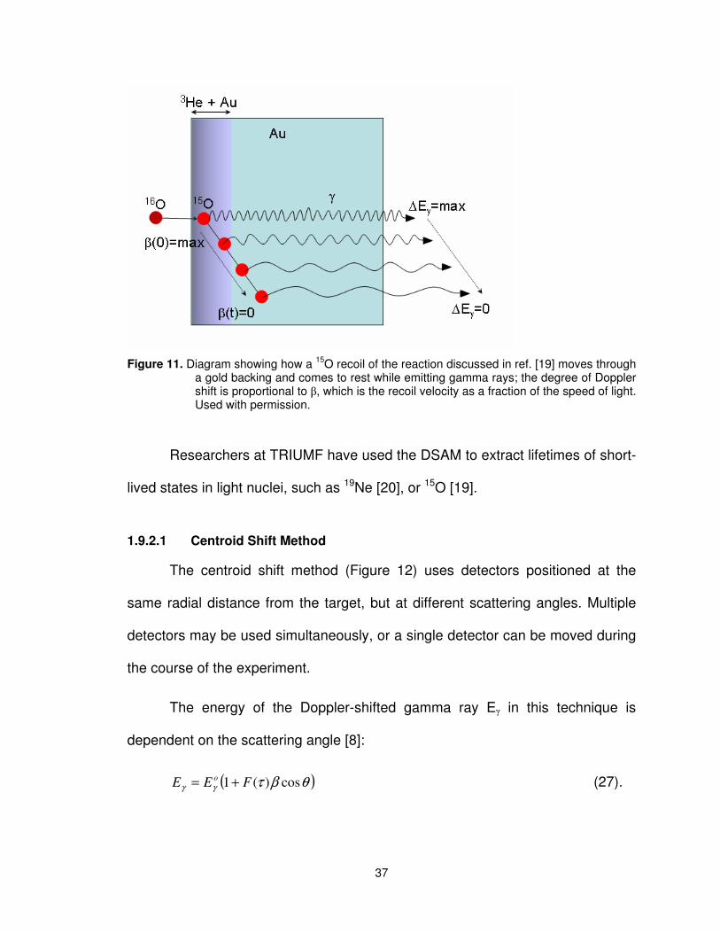
37
Figure 11. Diagram showing how a 15O recoil of the reaction discussed in ref. [19] moves through
a gold backing and comes to rest while emitting gamma rays; the degree of Doppler shift is proportional to β, which is the recoil velocity as a fraction of the speed of light. Used with permission.
Researchers at TRIUMF have used the DSAM to extract lifetimes of short-
lived states in light nuclei, such as 19Ne [20], or 15O [19].
1.9.2.1 Centroid Shift Method
The centroid shift method (Figure 12) uses detectors positioned at the
same radial distance from the target, but at different scattering angles. Multiple
detectors may be used simultaneously, or a single detector can be moved during
the course of the experiment.
The energy of the Doppler-shifted gamma ray Eγ in this technique is
dependent on the scattering angle [8]:
( )θβτγγ cos)(1 FEEo += (27).
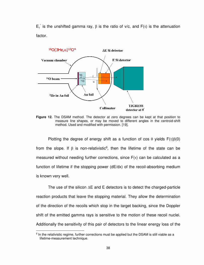
38
Eγ
° is the unshifted gamma ray, β is the ratio of v/c, and F(τ) is the attenuation
factor.
Figure 12. The DSAM method. The detector at zero degrees can be kept at that position to
measure line shapes, or may be moved to different angles in the centroid-shift method. Used and modified with permission. [19].
Plotting the degree of energy shift as a function of cos θ yields F(τ)β(0)
from the slope. If β is non-relativisticg, then the lifetime of the state can be
measured without needing further corrections, since F(τ) can be calculated as a
function of lifetime if the stopping power (dE/dx) of the recoil-absorbing medium
is known very well.
The use of the silicon ∆E and E detectors is to detect the charged-particle
reaction products that leave the stopping material. They allow the determination
of the direction of the recoils which stop in the target backing, since the Doppler
shift of the emitted gamma rays is sensitive to the motion of these recoil nuclei.
Additionally the sensitivity of this pair of detectors to the linear energy loss of the
g In the relativistic regime, further corrections must be applied but the DSAM is still viable as a
lifetime-measurement technique.

39
particles which strike them allows for setting gates on a desired charged particle
emission to isolate the reaction of interest. In the example in Fig. 12, the desired
charged particles were the outgoing alphas in the stripping reaction producing
15O in the gold target in which a layer of 3He was embedded.
1.9.2.2 Line Shape Analysis Method
Alternatively, in the DSAM a single detector can be mounted at a fixed
angle and radial distance away from the target (Fig. 12). The intrinsic HPGe
detector response and a calculated Doppler broadened line shape due to the
decay as the ions are slowing down can be used to determine the lifetime of the
state of interest, by means of Monte Carlo simulations and knowledge of the
stopping power (dE/dx) of the backing material.
Figure 13. Simulated gamma ray peaks emitted by a 6.791 MeV state in 15O of τ ≈ 2 fs – 3 ps in a
reaction of 16O with 3He at 50 MeV, with a gold backing material to stop the reaction products. The x axis is the Doppler shifted energy in keV; the y axis is intensity in arbitrary units. Image courtesy of Naomi Galinski.

40
Examples of calculated Doppler broadened lineshapes for various
lifetimes are shown in Figure 13, which simulates gamma ray emissions from a
6.791 MeV state in 15O, populated by a stripping reaction involving 16O with a
beam energy of 50 MeV bombarding a target of 3He implanted in Au. These
calculated peaks can be compared to experimental data to ascertain the lifetime
of the state.
1.9.3 Fast Timing Measurements with Scintillation Detectors
The measurement of nuclear lifetimes in the nanosecond to picosecond
range can be done by following radioactive decays of nuclei at rest, such as at
the 8π in TRIUMF. Overlap of time scales in the picosecond range allows fast-
timing delayed-coincidence methods to complement the RDM; however the
primary use of fast timing techniques is to extend lifetime measurements into the
nanosecond range, as the DSAM and RDM are not optimized for such long
lifetimes.
Prior to the discovery of the fast component of the light output from BaF2
crystals which established the usefulness of BaF2 detectors in measuring
lifetimes of short-lived nuclear excited states [21--23], fast timing measurements
were done by using combinations of NaI(Tl) and plastic scintillation detectors in
which beta-gamma coincidences could be measured, conversion electron and
gamma ray coincidences could be measured, or in the case of two plastic
scintillation detectors in coincidence, conversion electron-conversion electron
coincidences could be measured. The delayed-coincidence method was

41
successfully employed in the first measurement of the lifetime of the Iπ = 2+
excited state of 152Sm in 1955 [24], and in several measurements since then [25].
Collectively, these fast-timing delayed-coincidence methods come under
the heading of Fast Electronic Scintillator Timing (FEST). FEST can be applied to
various nuclear level schemes, as illustrated in Figure 14, ranging from simple
(Fig. 14(a)) to complex (Fig. 14(c)).
Figure 14. Decay schemes that can be handled by FEST. Varying levels of complexity are shown
here, with a) being the simplest, and b) and c) showing increased levels of complexity. Image courtesy of Paul Garrett.
The basic principle of FEST is that combinations of coincidence-correlated
events can be used to extract information about the nuclear excited state through
which those events transit. For example, Figure 14(a) represents a beta-gamma
event utilizing a plastic scintillator (for beta particles) and an inorganic scintillator
(for gamma rays). Figures 14(b) and 14(c) represent successively more complex
nuclear level schemes in which more versatile detector arrays can be used, such

42
as multiple scintillation detectors which can detect two gamma rays in succession
which transit through a state. Figure 14(b) shows that detecting γ2 in coincidence
with γ1 would yield the lifetime of the state labelled by τ1, as an example.
By combining an array of HPGe detectors and BaF2 detectors, the energy
spectra of radioactive daughter products can be acquired with the HPGe detector
array to gate transitions, while the BaF2 detector array can be used to measure
lifetimes. Trigger conditions can be set where gamma rays may be detected in a
sequence of HPGe-BaF2-BaF2 (an example of a triple coincidence) to set an
energy gate on a gamma ray which is known to feed a lower state, then using the
subsequently emitted gamma rays detected in BaF2 detectors to measure the
lifetime of a state which is populated in the cascade. This would be represented
by isolating γ4 in Figure 14(c) with an energy gate in an HPGe detector, then
requiring that two BaF2 detectors fire in coincidence; energy gates can be applied
onto the BaF2 detectors (though limited by their resolution) to further isolate the
cascade of interest, which would be that of γ2 followed by γ1.
A simpler trigger condition would be a BaF2-BaF2 coincidence condition, in
which two gamma rays in a nuclear cascade are detected; energy gates can be
used to isolate the state of interest if feasible.
The 8π array can be modified to use the beta-gamma method as briefly
discussed above, by means of a single plastic scintillator placed behind the beam
spot, as shown in Figure 17(c). Thus, the combination of DANTE and the plastic
scintillator would allow for isolation of excited states which are directly populated

43
in beta decay, which is advantageous if the structure of the daughter under study
is not well-known.
For the specific situation of 152Sm, its structure is well-known and the
gamma rays of interest are resolvable in a BaF2 detector. Furthermore, since the
decay process of interest involves electron capture, a plastic scintillation detector
was not mounted. Thus, coincidences between the BaF2 scintillators, or between
the HPGe and BaF2 scintillators, may be used. This will be discussed in more
detail in chapters 2 and 3.
1.10 ISAC at TRIUMF
Figure 15. The ISAC experimental hall (foreground) with the superconducting LINAC and ISAC-II
experimental hall (empty room, at back). The 8π apparatus is shown in the stopped-beam area along with the TRINAT, β-NMR and (now defunct) LTNO experimental apparatus. Image courtesy of Design Office, TRIUMF.

44
The Isotope Separation and Acceleration (ISAC) facility is shown in Figure
15. Several research groups conduct their activities with radiation detectors and
other equipment in this experimental hall, all of which depend on the production
of radioactive ion beams, produced via spallation reactions (which are the break-
up of the heavy nuclei into smaller ones under impact from small, energetic
projectiles) by bombarding 500 MeV protons on selected production targets.
Radioactive beams are produced at TRIUMF using the Isotope Separation
Online (ISOL) technique [26]. ISOL uses a mass separator dipole to deliver
beams of a given mass. After the mass separation, the beam is delivered to the
hall level where, in the case of the 8π, the beam, of a few tens of keV kinetic
energy, is stopped on the aluminized Mylar tape inside the 8π target chamber.
The radioactive ions, at rest, emit beta particles and gamma rays into the
detectors surrounding them.
1.11 The 8π at TRIUMF-ISAC
The 8π detector array at TRIUMF-ISAC consists of twenty HPGe detectors
in a truncated icosahedral arrangement [27]. The HPGe detectors are
surrounded externally by Bismuth Germanate (abbreviated to BGO; its formula is
Bi4Ge3O12) Compton-suppression shields; there are also internal BGO
suppressors which are directly behind the HPGe crystal. The HPGe detector
assembly is schematically depicted in Figure 16.

45
Figure 16. Cross-section of an HPGe detector at the 8π. Used with permission. [14]
The BGO detector suppression mode operates either in a hardware or
software veto configuration, in which a gamma ray detected in an HPGe detector
is not recorded if a scattered gamma ray is detected at the same time in the BGO
suppressors.
The HPGe detectors have 2.54 cm thick hexagonal Heavimet (an alloy
primarily consisting of Tungsten) collimators mounted directly in front of them,
with apertures approximately 2.5 cm in diameter. These collimators prevent
gamma rays from striking the external BGOs, thereby reducing false veto events.
The Heavimet also suppresses backscattering events, in which a gamma ray
scatters off one detector and enters the detector opposite, at lower energy.
Additionally, Delrin plastic shields may be mounted on the Heavimet collimators
to suppress Bremsstrahlung from high energy beta particles.

46
(a)
(b)
(d)
(c)
Figure 17. Clockwise from top left: (a) View of east half of the 8π array adjacent to the upstream half of the target chamber showing SCEPTAR. (b) PACES replacing SCEPTAR in the upstream portion of the target chamber. (c) The downstream half of the target chamber showing the Mylar tape and plastic scintillator. (d) The lead-shielded tape box attached to the downstream portion of the target chamber.
The arrangement of the HPGe detectors and their hexagonal collimators
leaves pentagonal gaps in the 8π frame, into which the DANTE detectors are
mounted. Additionally, because a cross-section through the 8π would reveal two

47
pentagonal configurations of the DANTE detectors, this is the origin of the name
Di-Pentagonal Array for Nuclear Timing Experiments.
When joined together, the two halves of the 8π frame form essentially 4π
solid angle coverage of the target chamber. The HPGe detectors themselves
subtend approximately 13% of the 4π solid angle [28].
The 8π HPGe and DANTE arrays surround a black Delrin target chamber
of approximately 16 cm diameter; a view of half the array around the upstream
half of the target chamber is shown in Figure 17(a). Inside this target chamber is
the Scintillating Electron Positron Tagging Array (SCEPTAR), which contains
twenty plastic scintillators designed in such a way that each plastic scintillator is
directly in front of an associated HPGe detector [29]. These detectors are
sensitive to beta particles and can be used to correlate beta decay events to
gamma ray events.
If internal conversion electrons need to be detected during an experiment,
the upstream half of SCEPTAR can be removed and replaced with the
Pentagonal Array for Conversion Electron Spectroscopy (PACES), as seen in
Figure 17(b). These are five circular silicon detectors capable of detecting
internal-conversion electrons.
Figure 17(c) shows the aluminized Mylar tape in the downstream half of
the target chamber. The Mylar tape forms a continuous loop through a lead-
shielded tape box, which can be seen in Figure 17(d). This shields the detector
array from activity on the tape if the experimental design requires periodic tape
movement to remove built-up activity from the beam spot.

48
CHAPTER 2: DETECTOR CHARACTERIZATION
2.1 Purpose and Overview
The 8π gamma ray spectrometer at TRIUMF has been optimized for
studying β-decaying nuclei, which populate excited states in their daughters that
emit gamma rays. The DANTE array of BaF2 detectors is well-suited to extend
the 8π’s capabilities. Adding lifetime measurement capability and high gamma
ray detection efficiency have motivated the integration of DANTE into the 8π.
Theoretical estimates show that BaF2 detectors are capable of reaching
an energy resolution of 7% of the 662 keV peak of the 137Ba daughter of 137Cs
[30]. Previous work has shown instrumental prompt response times on the order
of 290 picoseconds Full Width at Half Maximum (FWHM) of a coincidence timing
peak using BaF2 detectors [31].
Characterizing the properties of the TRIUMF-assembled BaF2 detectors to
be used in the DANTE array was done by first testing them individually in a
laboratory setup with 137Cs and 60Co sources.
2.2 The 8π DANTE Detectors
2.2.1 Detector Properties
The DANTE scintillation detectors consist of BaF2 crystals coupled to
Photonis XP2020/URQ fast photomultiplier tubes. Several characteristics of the
detectors were chosen to optimize DANTE for fast timing experiments, based on

49
previous work by Mach and Moszyński [22,23,32]. The crystal shapes were
designed for optimum light collection to obtain optimal energy and time resolution
[33], while the photomultiplier tubes were specifically chosen for their spectral
characteristics and fast rise times [23].
The BaF2 crystals are of cylindrical base diameter 40 mm, height 17 mm,
above which they are truncated cones of end-cone diameter 20 mm and height
30 mm. The total volume of each crystal is 12.5 cm3 [31].
Figure 18. Photoluminescent emission spectrum of BaF2. The energy of the light is on the x axis
in electron-volts, while the y axis is light intensity in arbitrary units. The dashed line marked “3” indicates the slow-component emission; the dotted line marked “4” is the fast-component emission. Both are at temperatures of 300 K; other lines in the graph correspond to cooler temperatures. The peak at 4.3 eV corresponds to approximately 300 nm; at 5.5 eV, it is ~225 nm. The peak at 6.4 eV corresponds to ~195 nm. Reprinted with permission. [34]
Like some other scintillator crystals, BaF2 has a two-component decay of
its fluorescence. The fast component, with a decay time constant of 600 ps, has
a wavelength of 220 nm and provides ~20% of the total light output of a pulse.
The slow component, with a decay time constant of 630 ns, has a wavelength of

50
310 nm and provides the remaining ~80% of the total light output [12]. The
photoluminescent emission spectrum of BaF2 is shown in Figure 18. It can be
seen that a third peak is detectable in the light emission of BaF2 at approximately
195 nm, but it is not of importance as it is likely to be partially absorbed by the
front faces of the photomultiplier tubes used for DANTE.
Figure 19. UV-Visible response curve for Photonis XP2020/URQ Photomultiplier tubes. The
radiant sensitivity (ratio of cathode current to visible light flux at a given wavelength) is on the y axis, wavelength on the x axis. [35]
The PMTs, which have bi-alkali photocathodes, were chosen to match the
light-emission characteristics of BaF2. The front faces are 52 mm in diameter and
are covered with fused silica glass. The operating voltage range is 2200 V to
3200 V. The pulse rise time is 1.4 ns, with a transit time of 27 ns, and transit time
spread of 150 ps [35]. The spectral characteristics, showing the wavelength
sensitivity of the XP2020/URQ, are shown in Figure 19.

51
An optical gel couplant is normally used with inorganic scintillation
detectors to protect the clear front face of the PMT and the base of the scintillator
crystal from scratching each other, as well as to fill in air gaps between the mated
surfaces to provide consistent transmission of light into the photocathode.
Additionally, optical couplants should have light transmission properties well-
suited to the intended application, in terms of spectral absorbance and refractive
index. In assembling the DANTE detectors, the optical couplant was specifically
chosen to have a similar refractive index to that of the front face of the PMTs, as
well as similar UV-Visible properties to those of the BaF2 crystals.
0
0.2
0.4
0.6
0.8
1
1.2
1.4
190 240 290 340 390 440 490
Wavelength (nm)
Ab
so
rban
ce
Figure 20. Absorption spectra of Dow Corning and specialized silicon-based optical gels. Higher
absorbance means less light is transmitted through the gel. The y axis is Absorbance (no units), while the x axis is the wavelength in nanometers. The feature in each of the curves at 340 nm is not a property of the gels; the apparatus changes detectors from UV to visible above 340 nm. Note the much higher ultraviolet cutoff of the conventional Dow Corning gel (blue triangles) versus the specialized gel (purple squares).

52
Figure 20 compares the UV and visible absorption spectra, which were
acquired on a Perkin-Elmer UV-Visible spectrometer at Simon Fraser University,
for a Dow Corning Q2-3067 optical gel, which is commonly used at TRIUMF for
scintillation detectors, and the specialized silicon-based gel used for the BaF2
detectors, provided by Henryk Mach. It can be seen that the conventional gel
would transmit the slow component but absorb the fast component, thus
degrading the timing resolution of the DANTE array.
2.2.2 Detector Assembly and Mounting
To assemble a DANTE detector, first the conical part of the crystal was
wrapped completely in white Teflon gauze to ensure light emissions would be
reflected through the base. Then the photomultiplier tube was oriented in an
upright position, and a minimum amount of the optical gel was placed on the
clear front face. After this, the crystal was carefully mated to the surface of the
PMT, using its own weight to spread the gel evenly. Finally, black electrical tape
was used to secure the crystal against the PMT, as well as electrically and
optically insulate the entire assembly. The detectors were then stored for ~24
hours to allow dark currents (induced by the exposure to ambient light) to decay
prior to testing. Figure 21 shows the components used to assemble a DANTE
detector, and Figure 22 shows a completely assembled detector in its test rig.

53
Figure 21. Components of a Barium Fluoride detector.
Figure 22. An assembled Barium Fluoride detector.
2.2.3 Laboratory Testing Regime
For initial testing, one or two detector(s) and associated electronics were
set up on a bench top in the ISAC-II counting room. The detectors were mounted

54
on metal frames, as shown in Figure 22, to allow for coincidence testing of two
detectors for timing measurements. The test rigs did not have the µ-metal shields
which were later used in the 8π during the experiment involving the 152Eu source.
These shields keep external magnetic fields from deflecting electrons away from
the dynode chain of the PMT. As discussed in Section 1.8, photoelectron
deflections away from the dynode chain would degrade the energy and timing
properties.
The specifications for the PMTs state that a parallel magnetic field of 0.12
mT, or a perpendicular field of 0.15 mT, will reduce detector gain by 50% [35].
The Earth’s magnetic field is approximately 0.5 Gauss, or 0.05 mT. Assuming
that the gain reduction is linear in proportion to the external magnetic field
strength, then the gain would be reduced by approximately 15%. This was
compensated by increasing the applied voltage by 15%.
2.2.4 Apparatus for Characterizing DANTE Detectors
In the lab, the assembled BaF2 detectors were connected to a CAEN high
voltage supply which was set to deliver approximately –2500 V to the PMTs. An
Ortec 4001C NIM crate was used to power and house analog electronic modules
during testing.
The block diagram for acquisition of energy spectra in the singles mode in
the laboratory environment is shown in Figure 23. Singles mode is the acquisition
of any signal from the detector regardless of origin (e.g. a gamma ray from a
source, or room background, or simply noise in the circuit). This mode is typically

55
used to acquire a high number of counts from a radioactive source when its
activity is much higher than background.
Figure 23. Equipment connections and pulse shapes for quantitatively determining energy
resolutions by means of a 137Cs source.
The dynode from the PMT emits positive pulses with exponential tails, with
rise times on the order of 2 ns and amplitudes between zero and ~50 mV,
depending on the energy of the gamma ray striking the BaF2 crystal. The Ortec
113 pre-amplifier shapes the sharply-rising pulse from the dynode, via a
combination of RC and transistor circuitry, into a smoother semi-Gaussian pulse
with an exponential tail. These pulses have amplitudes from zero to ~500 mV
with rise times of 100 ns, and are inputs to the Ortec 671 amplifier, set at a pulse
shaping time of 1 µs and with a coarse gain set to 100 or 200 to cover the range
from zero to 10 V (which corresponded to 0 to 1 MeV at a gain of 200, or 0 to 2
MeV at a gain of 100). The Ortec 671 then outputs these pulses to the Multi-
Channel Analyzer (MCA).
In the laboratory setup, a PC-based MCA with an analog to digital
converter (ADC) expansion card, allowing the digitization of analog signals, was

56
used to run a software package called Maestro. It can display and store spectra,
allowing for the export of these spectra for analysis after acquiring data.
Figure 24. Schematic of coincidence testing with a single channel analyzer for quantitatively
determining timing resolutions by means of a 60Co source.
The block diagram in Figure 24 shows the set-up of NIM modules for the
acquisition of data on timing characteristics in a coincidence-mode configuration
of the detectors. This requires two events to occur within a given time window; for
example, the emission of two gamma rays from a nucleus. This mode is typically
used when background activity is significant, and is well-suited for measuring the
lifetime associated with a two-step transition, be it a beta-gamma coincidence or
gamma-gamma coincidence. The detectors themselves are mounted a fixed
distance apart in a 180 degree arrangement.
The anode negative pulses from the voltage divider output have a rise
time of approximately 2 ns. The amplitudes of the pulses are dependent on the

57
applied voltage to the PMT, as well as the energies of the gamma rays striking
the BaF2 crystal. At –2500 V these pulses were typically between 0 and –7 V for
the energy range of 0 to 1.3 MeV.
Figure 25. A schematic overview of walk reduction using a CFD. Note the process of attenuating
the original signal, then inverting the input, delaying it, and adding it back to the attenuated signal.
The Ortec 935 Constant Fraction Discriminator (CFD) takes input negative
pulses between 0 and –10 V and outputs fast NIM-standard negative pulses of
adjustable width and approximate amplitude –1 V. An external delay cable may
be used with the CFD to adjust its time discrimination behavior. Usually, 3 ns
cables were used for the external delays during testing.

58
Constant fraction timing minimizes the energy dependence of time
measurements, called walk, by attenuating the input signal, and simultaneously
inverting and delaying the unattenuated signal, then adding this back to the
attenuated signal. Figure 25 shows this process at each stage of the constant
fraction timing method. The resulting output crosses over the baseline (“zero-
crossing time”) at a constant fraction of the original incoming pulse (i.e. it is
independent of the amplitude).
Some walk remains mainly due to slight differences in pulse rise times and
noise in the pulses, which can be reduced to a minimum by manual adjustment
of a potentiometer in the CFD. If it is set improperly it causes early crossover in
low-amplitude pulses and late crossover in higher-amplitude pulses. Once the
potentiometer is set properly, all pulses cross over the baseline at a zero-
crossing point which has as small a size as possible. Further removal of the
energy dependence of timing can be done by use of energy gating to reject
undesired timing signals.
The Ortec 935 CFD also has an adjustable lower-level discriminator,
which allows it to reject pulses below a certain energy. In the laboratory setup,
the threshold was normally set slightly above the noise level, unless a specific
testing regime required a higher setting.
The Ortec 566 TAC takes NIM-negative pulses at the start and stop
inputs, and can optionally be externally strobed to gate the output. The TAC
operates by opening a time window (this window is user-selectable, and for the
Ortec 566 it ranges from 50 ns to 2 ms) when it receives the start pulse. It waits

59
for a stop pulse to occur within the time window. Once it receives the stop signal,
it outputs a linear pulse whose amplitude is proportional to the length of time
between the detection of the start and stop signals.
In the laboratory testing phase the time window was set either to 50 or 100
ns. A 16 or 32 ns delay cable was placed between the CFD output of the “stop”
detector and the “Stop” input of the Ortec 566 Time to Amplitude Converter
(TAC). The “start” detector was connected with a short (~2 ns) delay cable to the
“Start” input of the TAC.
If the start and stop signals were to occur at the same fixed time apart,
then the TAC spectrum would have a delta function at that time interval. Further,
in timing spectroscopy, placing an external delay on the stop signal shifts the
timing peak into the middle of the spectrum where it is more convenient to
analyze, and also prevents the TAC from rejecting stop pulses occurring too
close in time to the start pulse due to its intrinsic start-to-stop conversion interval,
specified at 5 ns for the Ortec 566. This output can be monitored with an
oscilloscope or via a Multi-Channel Analyzer (MCA). However, there is
broadening of this delta function into a Gaussian distribution, attributable to
intrinsic limitations on the resolution of the detectors involved. The FHWM of the
peak is the time resolution due to the detector responses and the instrumentation
used to process the signals, and is one figure of merit to be optimized in a
coincidence experiment. Figure 26 shows the effect of distributing the start and
stop pulses in a Gaussian manner.

60
Figure 26. The input start and stop pulses are shown, with the TAC conversion of those pulses
shown below the solid black line. The TAC spectrum shown under actual conditions reflects Gaussian-distributed incoming CFD pulses.
To set up the energy gate as shown in Figure 24, the bipolar output of the
Ortec 671 amplifier was connected to the Tennelec 451 Single Channel Analyzer
(SCA). The SCA has adjustable lower and upper levels which can be set to their
extreme limits to open the energy gate, or they can be set at intermediate values
to permit only certain energy signals to be passed through. It outputs a positive
square pulse, which, in this setup, was routed to an Ortec 416A gate and delay
generator.
The Ortec 416A gate and delay generator, set to a 500 ns width, changes
the positive output pulse of the SCA to a negative input strobe of –6 V. The
purpose of using a gate and delay is to shift the strobe signal into the same time
range as the stop pulses entering the TAC, and therefore gate its output. The
Ortec 542 Linear Gate Stretcher is required to ensure the MCA reliably accepts

61
the linear pulses (which are different in shape than amplifier pulses) from the
TAC.
The procedure for setting up the SCA upper and lower limits is not shown
in Figure 24. This was done by passing the output of the Ortec 416A Gate and
Delay Generator to the MCA as a strobe and connecting the unipolar output of
the Ortec 671 amplifier to the input port of the MCA. The resulting spectrum was
visually examined to ensure acceptance only of the 1332 keV gamma ray from a
60Co source by adjusting the SCA (discussed in Section 2.2.6). After its lower
and upper levels were set, all the modules were re-wired back to the
configuration in Figure 24.
2.2.5 Energy Resolution Measurements
A 137Cs source was used in the lab to measure the energy-resolution
characteristics of the BaF2 detectors. This radioactive isotope’s decay scheme is
shown in the inset of Figure 27.
The usual practice for scintillation detectors is to quote their energy
resolution in terms of the ratio of the FWHM of the 662 keV peak from a 137Cs
source to the centroid of its position in a gamma ray spectrum [15].
Energy spectra were acquired from a 137Cs source mounted approximately
2-4 cm away from the end of the BaF2 crystal. The spectra were written to disk
for subsequent analysis with a program from the RadWare package, called gf3
[36], designed for analyzing gamma ray spectra, by fitting the peaks to obtain

62
centroids, areas and FWHMs. Typical gamma ray peaks are approximately
Gaussian in shape [12].
Figure 27. A typical 137Cs spectrum acquired in the singles mode in the lab with detector
DANTE04. The resolution of the 662 keV peak is 9.5% for this detector.
The 137Cs energy spectra were fitted and the centroid and FWHM of the
662 keV peak for each detector were obtained. A typical 137Cs energy spectrum
acquired using detector DANTE04 is shown in Figure 27. The resolution of the
662 keV peak in the spectrum was measured at 9.5%.
Additionally, a 60Co source was used, which has two cascading
photopeaks emitted by its daughter, 60Ni, as shown by the decay scheme inset of
Figure 28. The gamma ray spectrum of the 60Co source spectrum (Fig. 28)
indicates that a properly functioning BaF2 detector can resolve the two
photopeaks; at 1332 keV the resolution is approximately 9%. These spectra were
primarily used to qualitatively determine peak resolvability.

63
Figure 28. A typical 60Co spectrum acquired in the singles mode in the lab with detector
DANTE04. The resolution of the 1332 keV peak is approximately 9%.
2.2.6 Timing Resolution Measurements
The two cascading photopeaks of well-defined energy from 60Co are well
suited for use in coincidence experiments to establish detector timing
characteristics when the response is dominated by instrumental effects (the
states which de-excite have negligible lifetimes). The prompt timing resolution of
the detectors is measured by the FWHM of the TAC output signals.
The coincidence-mode setup shown in Figure 24 was used to first
examine timing behavior with a wide-open energy gate. This allowed the
investigation of adjustments to the CFDs and their effect on timing
characteristics. The two effects considered initially were the mode of operation
(which may be set to blocking or updating), and the effect of energy threshold
adjustment on the CFD.

64
(a)
(b)
Figure 29. Coincidence timing spectra from initial tests of the DANTE detectors in (a) the blocking mode and (b) updating mode, using a 60Co source without an energy gate. The FWHM of the peak in (a) is 253 ± 7 picoseconds, and in (b), 273 ± 11. Differing peak centroid positions are due to replacement of a loose connection on a delay cable.
The updating mode of operation of a CFD extends its output pulse if it
detects a second input signal from a detector closely following the initial signal.
By contrast, the blocking mode of operation will cause the CFD to ignore
incoming signals succeeding the initial signal for the duration of its output pulse.
It was found that the blocking mode of operation (Figure 29(a)) produced better
timing results than the updating mode of operation (Figure 29(b)). The updating
mode results in poorer timing characteristics due to increased probabilities of
acceptance of random coincidences.
It was found that raising energy thresholds to approximately 800 keV (as
determined from pulse heights on an oscilloscope) caused timing characteristics
to improve (Figure 30) as compared to operation with low thresholds (Figure
29(a)). This improvement is due to the elimination of low-energy contributions
due to Compton scattering. This energy dependence of timing behavior can

65
equivalently be reduced by using a Single Channel Analyzer (SCA) to set an
energy gate on the region of interest in a gamma ray spectrum, as discussed in
Section 2.2.4.
Figure 30. Coincidence timing spectrum from initial tests of the DANTE detectors in the blocking
mode, with high CFD thresholds corresponding to approximately 800 keV, using a 60Co source. The FWHM of this peak is 224 ± 4 picoseconds.
Figure 31. The energy gate region around the 1332 keV peak is shown with black bars in this
60Co spectum,
The energy gate region was set between approximately 1250 and 1400
keV (Fig. 31). The 1332 keV peak was used due to lower background

66
underneath this photopeak compared to the 1173 keV peak. This gate was set
on the detector producing the “stop” signal of the coincidence setup, since the
TAC does not have the facility of being easily strobed by two different SCAs. This
gating technique can also be done with computer software in analysis of
experimental data. Software gating is often more versatile than hardware gating,
if the data contains all the necessary information on an event by event basis to
usefully apply the energy gate.
The application of the energy gate produced a narrower time spectrum, as
shown in Figure 32. The effect of this energy gate proved to be similar to that of
applying high thresholds on the CFDs.
Figure 32. Coincidence timing spectrum using a 60Co source with an energy gate. The FWHM of
this peak is 221 ± 6 picoseconds.
Table 1 shows the energy resolutions and coincidence testing results for
all the available detectors tested under the laboratory conditions outlined
previously. These final results were found to be similar to reference data
collected from detectors borrowed from the University of Surrey, and qualified all
the DANTE detectors as being suitable for mounting in the 8π array. The average

67
time resolution was found to be 199 ps and the average energy resolution was
10.5% at 662 keV.
Table 1. The characteristics of the BaF2 detectors used in the 8π array after bench top testing. The first column refers to the numbering of the detectors in the 8π array. The second and third columns are serial numbers assigned to the PMTs and crystals by the manufacturers.
DANTE Det. #
PMT Serial #
Scionix Crystal Serial #
Energy Resolution at 662 keV (%)
Time peak FWHM (ps)
01 42036 0568 12.0 203.2 02h 42152 0565 N/A N/A 03 42138 0567 9.9 194.1 04 42186 0563 9.5 183.1 05 42205 0566 10.1 191.7 06 42222 0562 10.1 196.5 07 42225 0571 11.1 210.0 08 42228 0564 11.1 197.1 09 42232 0569 11.5 202.6 10 42233 0570 9.9 212.4
Further optimization of timing was also conducted by systematically
changing each CFD’s external delay cable length. Plotting the FWHM of the
prompt timing peak versus delay cable length showed identifiable minima. The
majority of detectors were found to operate best when their external delays were
2.8 to 3.2 ns long, with two outliers at 2.2 and 3.8 nanoseconds.
h This detector had been disassembled and so was not tested.
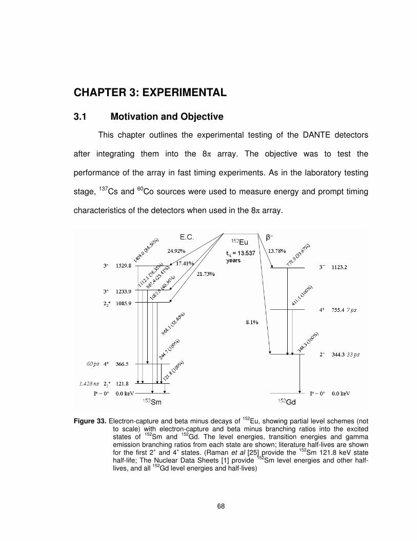
68
CHAPTER 3: EXPERIMENTAL
3.1 Motivation and Objective
This chapter outlines the experimental testing of the DANTE detectors
after integrating them into the 8π array. The objective was to test the
performance of the array in fast timing experiments. As in the laboratory testing
stage, 137Cs and 60Co sources were used to measure energy and prompt timing
characteristics of the detectors when used in the 8π array.
Figure 33. Electron-capture and beta minus decays of 152Eu, showing partial level schemes (not to scale) with electron-capture and beta minus branching ratios into the excited states of 152Sm and 152Gd. The level energies, transition energies and gamma emission branching ratios from each state are shown; literature half-lives are shown for the first 2+ and 4+ states. (Raman et al [25] provide the 152Sm 121.8 keV state half-life; The Nuclear Data Sheets [1] provide 152Sm level energies and other half-lives, and all 152Gd level energies and half-lives)

69
The performance of the DANTE array with regard to conducting
measurements of half-lives of nuclear excited states was tested with the
radioactive isotope 152Eu. It decays (Fig. 33) either by beta minus emission to
152Gd, or via electron capture to 152Sm, both of which are stable daughters.
The isotope 152Sm has an excited state (Iπ = 2+) at 121.8 keV with t½ =
1428 ± 17 ps [25], whose half-life was measured using the DANTE array. It will
be shown later that the measurement obtained using DANTE is more precise
than most previous measurements [25].
3.2 Integrating the DANTE Array into the 8π at TRIUMF-ISAC
3.2.1 Instrumentation Setup and Connections
The DANTE detectors were mounted in the 8π frame, and the dynode
outputs from their voltage dividers were connected to Ortec 113 pre-amplifiers for
each detector. These pre-amplifiers were then connected to Ortec 855 dual
amplifiers for processing dynode energy signals. The anode outputs were
connected to Ortec 935 quad CFDs for processing timing signals. All three
outputs available from each CFD in the Ortec quad module were used. One of
the outputs was connected to the start input of an Ortec 566 TAC, which was not
externally strobed. The second output was connected to a LeCroy 429A FIFO
(Fan-In/Fan-Out) module, which fed signals to an Ortec CO4020 four-input logic
module that is hardware-designed to do OR logic and send stop signals to the
TACs (Figs. 34 and 35). The logic modules were set to prevent detector self-
timing. The third output of the CFD sent signals to trigger logic circuitry which

70
gated the associated ADC readouts. The energy threshold of the CFD was used
to remove noise triggering from the timing and energy readouts in the electronics.
The width of the output pulse from each CFD was set to 200 ns.
Figure 34. Simplified schematic of signal flow in the 8π with four BaF2 detectors operating. The
flow of data is shown up to the readout of the ADCs.
Figure 34 shows the input and output connections of the FIFO and logic
modules for the full array of ten DANTE detectors, although at the time of the
experiment, only four of the ten were fully-instrumented as shown in Figure 35.
The remaining input connections to the FIFOs for detectors 5 through 10 were
not used, though all outputs from the FIFOs were connected as inputs to the
logic modules stopping detectors 1 through 4.

71
Figure 35. Schematic showing input connections to the FIFOs (dark circles). Output connections
from the FIFOs correspond to inputs on the logic modules and/or other FIFOs. Note that the output for detectors 1-4, 9 and 10 has been labelled “A” for convenience. On the logic side, inputs are shown (open circles represent the input for a detector which has had self-timing blocked in the logic; otherwise it would start and stop its own TAC) with outputs labelled as Stop cables to the TACs for each detector.
The TAC and amplifier outputs were connected to Ortec AD413A ADCs,
which are Fast Encoding Readout ADC (FERA) bus compatible modules,
capable of binning digitized data into 8192 channels. Energy and time signals
can be read out from these modules on an event by event basis.
3.2.2 The 8π MIDAS Data Acquisition System
At TRIUMF, data acquisition is done using a program called the Maximum
Integrated Data Acquisition System (MIDAS) [37], with a web-based interface as
shown in Figure 36. MIDAS controls subprograms which acquire different
streams of data from the ADCs connected to the various detectors in the 8π

72
array. These raw data streams are written to computer disk in binary format if the
user sets an option to do so. MIDAS also interfaces with the Experimental
Physics and Industrial Control System (EPICS) [38] which is used to display, in
real time, scaler readouts from the 8π detectors. It is also used with a slow
control system to monitor vacuum pressure, electronics shack temperatures, etc.
Figure 36. The MIDAS control window, showing a typical situation in which a run has been
stopped, but otherwise all aspects of the DAQ are operational except for EPICS.
MIDAS utilizes an Online Database (ODB), which contains experimental
parameters alterable on a run by run basis. The ODB contents are written to disk
each time a new run is initiated. Some important parameters include the run

73
number, time stamp, trigger condition, beam cycle time, tape movement cycle,
etc. Most of the parameters can be modified as desired by the useri.
An analyzer program, which is part of MIDAS, performs histogramming of
spectra recorded from FERA modules connected to the SIS301 Versa Module
Europa (VME) crate in the 8π electronics shack. In the online mode, it runs in
conjunction with the other programs that MIDAS controls. In the offline mode, this
program can be run to reprocess (play back) binary data streams from the
computer disk, which contain all the events which were recorded under a given
trigger condition. This analyzer code was used for subsequent post-experiment
analysis of data from the decay of 152Eu.
3.2.3 Calibration of TACs
The TACs were set to 100 ns time windows. The 8π DAQ (like the PC-
based MCA) processed TAC output signals into spectra with discrete bins of
8192 channels, with nominal bin sizes of 12.21 picoseconds per channelj. To
account for instrumental effects, an Ortec 462 time calibrator was used to
determine the actual bin size for each TAC. This module outputs start and stop
pulses which produce delta functions. A dispersion amplifier in the calibrator
produces stop signals spread in a Gaussian distribution to enable a more precise
determination of the centroids of the timing peaks. The Ortec 462 module has a
specified calibration uncertainty of ±10 ps per 10 ns period, producing a 0.1%
systematic uncertainty. It was set to a period of 0.01 µs and a range of 0.08 µs,
i In principle, all of them (even the run number) could be changed at any time but it is likely that
changing such parameters in the middle of a run would render that run’s data set unusable. j Dividing 100000 picoseconds (100 nanoseconds) by 8192 channels = 12.21 ps/ch.

74
outputting pulses over a 20 – 100 ns range, separated by 10 ns for each TAC
being calibrated. This is similar to the time distribution of the TAC spectra during
the 152Eu experiment.
Figure 37. TAC calibration spectrum for TAC 1 in the 8π electronics shack.
Two calibrations were performed; one was undertaken two weeks prior to
the experiment and a second one immediately after the experiment. The results
for the second calibration are reported here. There was an overall drift of ±0.009
ps/channel between the first and second calibration, included as a systematic
contribution in the uncertainties reported here.
The calibration spectrum for TAC 1 is shown in Figure 37. Other TACs
showed similar spectra. Peak centroids were determined by Gaussian fits, after
which a weighted linear regression of centroid channel number against time was
used to determine the TAC bin size in picoseconds per channel. The TACs in the

75
8π electronics shack binned time events at ~12.5 picoseconds per channel;
detailed results are shown in Table 2.
Table 2. Results of TAC calibrations. The total error adds, in quadrature, the statistical error, TAC drift, and the intrinsic accuracy of the TAC Calibrator and converts to an absolute error.
TAC Slope (ps/ch)
Statistical Unc. (ps/ch)
TAC Calib. Unc. (ps/ch)
TAC Drift Unc. (ps/ch)
Total Unc. (ps/ch)
1 12.5963 0.0029 0.013 0.009 0.016 2 12.4876 0.0019 0.013 0.009 0.016 3 12.4238 0.0038 0.013 0.009 0.016 4 12.5968 0.0018 0.013 0.009 0.016
3.3 Experimental Run
3.3.1 Preparation of Software and Instrumentation
A 60Co source, mounted at the beam-spot position of the 8π target
chamber, was used for calibration purposes to measure timing characteristics
dominated by instrumental effects and to check TAC drift. The 60Co data was
analyzed to check for any degradation in the detectors between the lab testing
phase and mounting of the DANTE detectors in the 8π.
The results from using the 60Co source yielded an average FWHM of 270
± 8 picoseconds in the timing peaks; details are noted in Table 3. These results
were obtained by applying a software double energy gate, requiring that one
detector of a coincidence pair detect an energy signal in range 1 of Figure 38,
and that the other one detect an energy signal in range 2. Only then was the
event accepted in the time spectrum for that coincidence pair.
Although the time resolutions obtained were slightly worse than those
obtained in the lab testing phase, they did not differ appreciably from one another

76
when the detectors were mounted in the 8π. This is not unexpected, given the
presence of longer cables and more complex instrumentation of the 8π array.
Figure 38. The regions “1” and “2” of this 60Co energy spectrum show the two energy gates
taken, one in each detector of a coincidence pair, to establish prompt timing characteristics in the 8π for the DANTE detectors.
Table 3. The characteristics of the BaF2 detectors used in the 8π array at the time of the 152Eu experiment. Timing resolutions are quoted only for detectors actually used in the experiment. Compare to Table 1.
DANTE Det. #
PMT Serial #
Scionix Crystal Serial #
Energy Resolution at 662 keV (%)
Time peak FWHM (ps)
01 42036 0568 12.0 N/A 02k 42152 0565 N/A N/A 03 42138 0567 9.5 268 04 42186 0563 9.1 242 05 42205 0566 10.9 N/A 06 42222 0562 9.7 N/A 07 42225 0571 11.4 259 08 42228 0564 11.9 271 09 42232 0569 10.0 N/A 10 42233 0570 11.3 N/A
k This detector was not mounted in the array.

77
The energy resolutions of the DANTE detectors were measured using a
137Cs source to check for degradation of energy resolution. The results are
summarized in Table 3. In general there did not appear to be a systematic effect
on energy resolution; some detectors had slightly improved resolutions while
others had slightly degraded resolutions, compared to the lab test results.
The Ortec 935 CFD energy thresholds were set slightly above the noise
level, which corresponded to approximately 30 keV. The CFD walks were
adjusted, as explained in section 2.2.4, to ensure optimal timing characteristics.
The Ortec 855 amplifier gains were set to produce output energy signals over the
range of zero to 2 MeV, corresponding to approximately 0.25 keV per channel.
Figure 39. The east (a) and west (b) halves of the 8π are shown with numbered cylindrical-
conical crystals (brown) showing the placement of the DANTE detectors in the gaps of the existing HPGe array’s frame, as well as the BGO Compton suppressors (red), Heavimet collimators (blue) and HPGe front faces (green). Images courtesy Smarajit Triambak.

78
The four detectors which were used in the coincidence timing
measurements have two numbering schemes. One scheme is their physical
positioning in the array as shown in Figure 39(a) and 39(b). A second scheme,
used in the post-experiment processing and 8π DAQ, relates the physical
positioning to the alternate numbering, denoted by the numbers in parentheses in
Fig. 39(a) and (b) and in Table 4. The detectors will be exclusively referred to by
the second scheme for the remainder of this thesis.
Table 4. Correlation between physical detector placement and logical detector numbering in the post-experiment analysis.
Physical Detector Logical Detector
DANTE07 Det #1
DANTE08 Det #2
DANTE03 Det #3
DANTE04 Det #4
3.3.2 Experimental Data Acquisition
A 60Co source, as mentioned previously, was used to monitor TAC drift
between the start and end of the experiment. It was found that the prompt timing
peaks shifted by approximately 1.4 ± 0.4 channels between the beginning and
end of the experiment. This had a negligible effect on the results obtained.
During the course of the experiment, both singles and coincidence mode
data were taken with the 152Eu source mounted at the beam-spot position of the
8π target chamber. The singles mode data was taken once per day to check for
amplifier gain drift. The coincidence mode data (usually taken over a 24-hour
period between singles runs) was used for timing measurements. TAC drift was
negligible during the experiment. This was qualitatively assessed by overlaying

79
the TAC spectra from different runs. On the other hand, energy spectra exhibited
sizable gain drifts due to temperature fluctuations. Some high-energy gamma ray
peaks drifted by up to 25 keV between some runs. This effect was corrected in
software.
The coincidence mode trigger logic allowed for double coincidences of two
BaF2 detectors. Alternatively a triple coincidence between one HPGe detector
and two BaF2 detectors was accepted. The BaF2-BaF2 coincidence data was
used to measure lifetimes, while the HPGe-BaF2-BaF2 coincidences can be used
to place an energy gate on a known gamma ray in the cascade of 152Sm to
attempt to improve lifetime measurementsl.
A total of 30 million coincidence events were recorded; the BaF2-BaF2
doubles events (including those in which the HPGe array provided the initial
trigger) were used to construct the spectra used in offline analysis via the
analyzer.
l This technique was not used, owing to very poor statistics when attempting this gating method.

80
Table 5. Simplified structure of a BaF2-BaF2 coincidence event, showing the portions relevant to the analysis of lifetimes.
Number of Amplifier ADC signals
Number of TAC ADC signals
Detector Event Type
Detector # i Detector # j
ADC number i ADC number j
Energy readout from ADC Energy readout from ADC
TAC number i TAC number j
TAC readout via ADC TAC readout via ADC
BaF2-BaF2 coincidence events are those in which any two detectors
numbered i and j (i ≠ j, where i = 1…4, j = 1…4) sent signals to the DAQ. There
are six unique combinations of coincidence pairs: (1, 2), (1, 3), (1, 4), (2, 3), (2, 4)
and (3, 4). Table 5 outlines the important components of the event structure.
3.4 Post-Experiment Analysis
3.4.1 Gain Matching
As mentioned in the previous section, the peak centroids in the ADC
spectra from HPGe and BaF2 detectors were found to drift over the course of the
experiment. This was mainly due to temperature-dependent gain drift in the
HPGe and BaF2 detector amplifiers and photomultiplier tube gain drift for the
BaF2 detectors.
Before the start of the experiment, the 60Co source was used to initially
gain match the BaF2 and HPGe detectors using the 1173 and 1332 keV peaks,
so that all the ADC spectra showed peaks at the same channel numbers.
However owing to the above-mentioned drift during the experimental run, off-line
software correction (gain matching) of the spectra was required. Successful gain

81
matching results in complete alignment of the gamma rays in all energy spectra
summed over all runs.
For this procedure, first the raw ADC spectra from the individual detectors
were extracted on a run by run basis. Then, gamma ray peaks from the 152Eu
source with precisely-known energies were Gaussian fitted and their centroids
were recorded.
The next step was to use a quadratic fit,
nnnn oxgxaE ++= 2 (28),
to conduct a weighted regression of peak energies versus their centroids. The
resulting fit coefficients were stored on a run by run basis, with each detector
having its own set of gain correction coefficients.
In equation 28, for the nth detector, En is the gain matched energy, x is the
channel number, an represents the nonlinearity term, gn represents the gain, and
on represents the offset. Quadratic fits were used for gain matching both HPGe
and BaF2 ADC spectra. The nonlinearity term for BaF2 detectors was found to be
negligible, being on the order of 10-6 keV/channel2.
3.4.2 Half-Life Measurements
3.4.2.1 Selection and Application of Energy Gates
The data from the experiment and the code to analyze the data were
copied to a separate computer for offline re-analysis. Several modifications were
made to this offline analyzer program, which are discussed later in this section.

82
The purpose of the experiment is to determine the half-life of the 122 keV
state in 152Sm, using the gamma ray of the same energy in coincidence with
gamma rays that feed the state. Coincidence events consist of one detector
detecting a 122 keV gamma ray while the other detector detects gamma rays
which feed the state from above, as seen by following the decay scheme in
Figure 33. Since the gamma rays are well-separated in energy, the method of
double energy gating can be used, similar in principle to that employed on 60Co
spectra, as discussed in Section 3.3.1.
Figure 40. A gain matched coincidence mode spectrum from detector #4 in coincidence with
detector #1, 2, or 3, labelled with gamma ray energies in keV. The black bars show the chosen energy gate region which was applied to that detector to extract time spectra. The region below 70 keV has been omitted.
In order to apply double energy gates, the analyzer program was modified
to output gain matched energy spectra for all unique detector coincidence pairs
by using the gain coefficients extracted via the procedure discussed in section
3.4.1. The energy gating region about the 122 keV peak associated with the

83
transition was selected from the gain-matched spectra (Fig. 40). The effect of
Compton scattering from higher-energy gamma rays was established by
comparing the ratio of peak to background areas for the full peak width and for
the region covered by the energy gate, which was approximately over the range
of the FWHM.
The ratio of peak to background area for the full peak width at 122 keV
was 1.164 ± 0.005, while the peak to background over the FWHM range was
1.372 ± 0.007. The Compton scattering contribution to the prompt timing was
thus reduced by approximately 15% by applying the stringent energy gate as
shown in Figure 40 by the black vertical lines.
After setting the energy gate, the coincidence mode data sets were sorted.
During the sorting, the analyzer created data files consisting of energy-gated
energy-time matrices (which are two-dimensional file structures in which the y
axis contains energies and the x axis, TAC signals). In the case of the detector
pair used as an example in this section, the energy-gated time signals from
detector #4 and the energies recorded by detector #3 were binned in an E vs. T
matrix, referenced in terms of the (x, y) axes of the matrix as a (T4, E3) matrix.
More generally, these matrices are labelled as (Tj, Ei) for a gate on the 122 keV
transition seen in Ej, where i and j have been defined in Section 3.3.2.
The energy-time matrices were written in a format which could be read in
by gf3m, a modified version of gf3 [39]. Twelve separate energy-gated matrices
were written, which consisted of events associated with gated (Tj, Ei) pairs,
ranging from (T1, E2) to (T4, E3).

84
The y-projection of the energy-time matrix, as shown in Figure 41 from the
(T4, E3) matrix, shows the gated energy spectrum for detector #3. As expected,
the intensity of the 122 keV peak has been reduced. The remaining intensity of
the peak in the gated spectrum shows that there were events where Compton-
scattered gamma rays from higher energy peaks entered the 122 keV gate on
detector #4 in coincidence with the 122 keV transition in detector #3.
Further, the noticeable reduction in intensity of the 344 keV peak,
associated with the 152Gd daughter of 152Eu shows that the energy gate applied
to the 122 keV transition was largely effective in removing contributions from that
daughter’s excited states.
Figure 41. The energy spectrum projected out for detector #3 after gating on the 122 keV gamma
ray in detector #4. The black lines represent two energy gate regions, a narrow energy gate taken around the 244 keV peak (region 1) and a wider energy gate from approximately 200 keV to 1500 keV (region 2). The region below 70 keV has been omitted.
The second energy gate was set, after projecting the y axis of the matrix
file, either in a region around the 244 keV gamma ray (which is the gamma ray

85
which directly feeds the 122 keV state), or on a region from 200 to 1500 keV,
both of which are shown in Figure 41. The time projection from the (T4, E3) matrix
with the wider energy gate is shown in Figure 42.
Figure 42. The time spectrum from the (T4, E3) matrix after double gating the 122 keV transition
in detector #4 and the 200-1500 keV range in detector #3.
3.4.2.2 Fitting Time Spectra to Obtain Half-Lives
After the double gate was applied, the resulting projected time spectra
were written to disk as ASCII files for input to a fitting algorithm modified from
one originally designed for precision half-life measurements for the superallowed
beta-decay program conducted by the 8π group at TRIUMF [14,40,41]. The
program, called 8pifit, is designed to determine half-lives via a χ2 minimization
process of initial guesses provided to it.
In the limit of a large number of counts in each bin of a time spectrum,
each data point has a randomly distributed uncertainty equal to the square root of
the value in that bin; this assumes the uncertainty is distributed in a Gaussian

86
fashion. This is not a good approximation when the number of counts is not very
large, and is a result of Poisson statistics governing radioactive decay rather than
Gaussian statistics. In such cases, the error is best expressed by the ‘maximum
likelihood’ and the fitting program described previously was designed specifically
to calculate data point errors by that method. An excellent overview of the use of
maximum likelihood in fitting experimental data is described by M. Trinczek [42],
as well as G. F. Grinyer [40].
The program conducts a χ2 minimization using the Marquardt-Levenberg
algorithm [43] after being provided with initial guesses for parameters of a fit
function. It reads in the data set from the time spectrum and outputs a half-life
based on the fit function
BkgeAtft
o += −λ)( (29).
Table 6. Parameters for half-life measurements using the fit function in equation 29.
Parameter Initial Value Description
Ao Extrapolated to t = 0 by 8pifit Normalization constant
λ ln(2) / 1450 ps = 0.0004780 ps-1 152Sm decay rate
Bkg 0.1 counts/ps TAC random coincidences
Table 6 describes the free parameters used for the half-life measurements
and their initial values. Convergence to a result was required prior to 500
iterations. The 8pifit program displayed the following outputs for each time
spectrum that was fitted:
• The fitted value half-life and uncertainty,
• The background level, which was typically on the order of 0.01 counts per
picosecond,
• The χ2/ν of the fit, which was typically very close to 1.

87
Deconvolution of the prompt peak from a decaying exponential component
is more challenging. Therefore, the technique of channel chopping was employed
to determine the region of the fit in the time spectrum where half-life
measurements are not affected by prompt or instrumental contributions.
To employ the technique of channel chopping, first the data in the time
spectrum from Figure 42 was reversed.
Figure 43. A typical exponential fit of the time spectrum in Figure 42. The time base is 12.49 ±
0.02 ps/channel. The half-life was measured to be 1478 ± 17 ps. The χ2/ν of this fit is 0.97.
The reversing of the data set was required to correctly fit it using the
model expressed in equation 29. Figure 43 shows a typical range over which the
spectrum was fitted. The region over which the fits were made was chosen to
ensure that the decay is exponential in nature with only the constant background
contributing to the activity being measured.

88
The instrumental response also affects the time spectrum in a non-
negligible fashion when the activity of the excited state reaches background
levels. The end channel of a fit region must be chosen such that this instrumental
influence does not affect the precision of the measurement of the half-life.
The systematic chopping of channels was done by choosing an initial
range from the prompt peak to 1000 channels after it. Channels were removed
from the beginning of the fit in steps of twenty channels at a time. The half-life
was determined each time. Figure 44 shows the influence of the prompt
contributions to half-life measurements.
1300
1350
1400
1450
1500
1550
0 50 100 150 200 250 300 350 400 450
Channels Chopped
Ha
lf-l
ife (
ps)
Figure 44. Graph showing the effect on the half-life of removing channels from the beginning of
the range of the time spectrum shown in Figure 56 to use with an exponential fit. The step size was 20 channels removed per fit iteration.
A similar process was undertaken to determine the effect of removing
channels from the end of the time spectrum, by fixing the start channel at 300

89
channels after the prompt peak, and chopping from the end channel
systematically. Initially the end channel number was set at 1200 channels after
the prompt peak. Figure 45 shows the effect of instrumental response on the
half-life measurement.
1300
1350
1400
1450
1500
1550
0 50 100 150 200 250 300 350 400 450
Channels Chopped
Ha
lf-l
ife (
ps)
Figure 45. Graph showing the effect on the half-life of removing channels from the end of the
range of the time spectrum in Figure 56 to use with an exponential fit. The step size was 20 channels removed per fit iteration.
After the channel chops were done for all double energy-gated time
spectra for the twelve detector combinations, it was found that when chopping
channels from the beginning of the time spectra, stabilization of the
measurements occurred no later than 260 channels after the prompt peak for any
detector combination. When chopping channels from the end of the time spectra,
the half-life measurements remained stable well into the middle of the time
spectra.

90
The differences in the nature of the stabilization between Figures 44 and
45 (which are representative of the general channel-chopping results for all time
spectra) show that the half-life measurements are insensitive to instrumental
effects when doing repeated channel chopping from the end of the fit region. By
contrast, repeated channel chopping from the beginning of the fit region shows
that the half-life measurements are very sensitive to prompt and instrumental
contributions at the beginning of the time spectrum, so this technique is
particularly valuable for determining the best ranges for the fit regions in order to
measure the half-life of interest.
3.4.2.3 Results of Fitting Time Spectra with a Wide Energy Gate
Table 7 shows the effect of changing both the start and the end channels
in a systematic manner, keeping the same number of channels for all twelve fits.
The individual detector pair results are reported along with weighted averages
whose uncertainties have been increased by multiplying them by the square root
of the χ2/ν, if larger than one (as recommended by the Particle Data Group [44]),
prior to reporting the final results. This adjustment accounts for systematic
contributions to the data sets whose origin is not immediately identifiable.
When taking a wide second energy gate from 200 – 1500 keV, the fit
ranges from 300 past the prompt peak to 1000 or 1100 channels yielded data
sets with χ2/ν values of 3.09 and 2.98, respectively. By comparison, the fit ranges
from 400 to 1000 or 1100 channels resulted in data sets with χ2/ν values of 0.91
and 1.11, respectively. This indicates that variation of the start channel has a
systematic effect, but variation of the end channel does not. This is also borne

91
out by the intermediate χ2/ν value of 1.43 for the intermediate fit range of 350 –
1050 channels.
Table 7. Summary of half-lives and errors for various fit ranges using a wide energy gate. Each range is the start and stop channel number relative to the location of the TAC prompt peak. Errors in the weighted averages are the statistical errors adjusted for the χ2/ν of the data sets.
Detector Pair
Half-Life (ps)
(300 to 1000)
Half-Life (ps)
(300 to 1100)
Half-Life (ps)
(350 to 1050)
Half-Life (ps)
(400 to 1000)
Half-Life (ps)
(400 to 1100)
1v2 1468.8 ± 15.2 1449.5 ± 12.7 1434.4 ± 17.1 1425.4 ± 24.5 1405.4 ± 19.5
1v3 1486.8 ± 16.9 1472.4 ± 14.1 1448.2 ± 18.9 1450.7 ± 27.6 1437.0 ± 22.0
1v4 1396.4 ± 14.2 1412.2 ± 12.2 1436.6 ± 17.6 1391.6 ± 24.4 1420.1 ± 20.2
2v1 1435.7 ± 15.2 1438.5 ± 12.9 1454.6 ± 18.1 1419.1 ± 25.4 1426.7 ± 20.6
2v3 1453.1 ± 16.0 1457.8 ± 13.5 1448.7 ± 18.6 1440.4 ± 27.0 1452.8 ± 21.9
2v4 1424.9 ± 15.0 1431.4 ± 12.7 1450.0 ± 17.9 1425.3 ± 25.6 1435.0 ± 20.7
3v1 1425.7 ± 14.3 1437.8 ± 12.1 1421.4 ± 16.6 1416.1 ± 24.3 1441.0 ± 19.8
3v2 1414.2 ± 13.9 1426.2 ± 11.9 1419.0 ± 16.4 1408.8 ± 23.9 1432.0 ± 19.6
3v4 1478.0 ± 16.7 1482.1 ± 14.0 1493.3 ± 19.9 1495.0 ± 29.0 1497.2 ± 23.0
4v1 1426.6 ± 14.3 1416.1 ± 12.0 1423.8 ± 16.7 1439.8 ± 24.8 1417.3 ± 19.6
4v2 1440.7 ± 15.2 1437.8 ± 12.9 1420.5 ± 17.5 1443.2 ± 26.2 1438.7 ± 21.1
4v3 1456.8 ± 15.9 1462.9 ± 13.4 1459.5 ± 18.6 1429.8 ± 26.3 1447.4 ± 21.4
Wt. Avg 1440 ± 8 1442 ± 6 1440 ± 6 1430 ± 7 1436 ± 6
χ2/ν 3.09 2.98 1.43 0.91 1.11
The half-life values themselves and their weighted averages are not
statistically different from one another within their overlapping uncertainties,
showing that the measurements are valid over different fit ranges within the limits
established by the channel chopping method. The weighted average of twelve
independent measurements from the rightmost column of Table 7 is shown in
Figure 46. The rightmost column has a χ2/ν = 1.11, and yields a half-life of 1436 ±
6 picoseconds.

92
1405.4
1420.1
1452.8
1497.2
1417.3
1447.4
1432.0
1438.7
1426.71435.0
1437.0 1441.0
1300.0
1350.0
1400.0
1450.0
1500.0
1550.0
1v2 1v3 1v4 2v1 2v3 2v4 3v1 3v2 3v4 4v1 4v2 4v3
Detector Pair
Half
-lif
e o
f 121 k
eV
sta
te (
ps
)
Figure 46. Graph of data from the rightmost column of Table 7. The weighted average and its
error bars are shown by the black and dashed lines, respectively. The data set has χ
2/ν = 1.11.
3.4.2.4 Results of Fitting Time Spectra with a Narrow Energy Gate
A similar process of channel chopping was done on time spectra extracted
using a narrower energy gate on the 244 keV peak only (refer to Figure 41 for the
region of this narrower gate). The projected time spectrum from the (T4, E3)
matrix using this double-gating method is shown in Figure 47(a). A representative
fit of the reversed time spectrum is shown in Figure 47(b). Examples of the effect
of channel chopping are shown in Figures 47 (c) and (d).

93
(a)
(b)
1300
1350
1400
1450
1500
1550
1600
0 50 100 150 200 250 300 350 400 450
Channels Chopped
Half
-lif
e (
ps)
(c)
1300
1350
1400
1450
1500
1550
1600
1650
1700
1750
1800
0 50 100 150 200 250 300 350 400 450
Channels Chopped
Half
-lif
e (
ps)
(d)
Figure 47. (a) Time spectrum from the (T4, E3) matrix after double gating the 122 keV transition in detector #4 and the FWHM of the 244 keVpeak in detector #3. (b) Typical exponential fit of the spectrum in (a) with time base 12.49 ps/channel; measured t½ = 1473 ± 43 ps. (χ2/ν of fit = 0.98). (c) Effect on half-life due to removing channels from the beginning of the range of data in (b). (d) Effect on half-life due to removing channels from the end of the range in (b).
The energy gating method in which only the regions of 121 and 244 keV
are used produced results with essentially no systematic contribution, as
evidenced by the χ2/ν values for all five fit regions chosen, shown in Table 8.
Figure 48 shows a plot of the rightmost column of the table. While this method
better isolates the gamma rays of interest, the uncertainties in the results are
larger due to lower statistics at each data point.

94
Table 8. Summary of half-lives and errors using narrower double energy gates. Each range given is relative to the location of the TAC prompt peak. Errors in the weighted averages are the statistical errors adjusted for the χ2/ν of the data sets.
Detector Pair
Half-Life (ps)
(300 to 1000)
Half-Life (ps)
(300 to 1100)
Half-Life (ps)
(350 to 1050)
Half-Life (ps)
(400 to 1000)
Half-Life (ps)
(400 to 1100)
1v2 1449.7 ± 39.5 1428.5 ± 33.0 1393.5 ± 42.7 1308.1 ± 56.1 1310.0 ± 46.4
1v3 1486.9 ± 46.1 1479.4 ± 38.3 1459.2 ± 50.8 1372.7 ± 67.6 1389.9 ± 55.5
1v4 1381.4 ± 39.0 1426.5 ± 34.1 1490.0 ± 52.6 1406.6 ± 69.5 1481.6 ± 58.9
2v1 1408.8 ± 39.8 1420.1 ± 33.9 1439.4 ± 47.7 1393.8 ± 67.1 1415.9 ± 55.1
2v3 1369.6 ± 37.9 1396.8 ± 32.8 1361.5 ± 43.9 1382.1 ± 67.4 1432.9 ± 56.5
2v4 1432.7 ± 42.4 1470.8 ± 36.2 1452.0 ± 49.6 1380.1 ± 67.8 1458.8 ± 57.3
3v1 1418.0 ± 37.2 1388.3 ± 31.1 1378.0 ± 42.5 1437.4 ± 65.0 1380.5 ± 50.5
3v2 1474.8 ± 39.6 1485.2 ± 33.2 1496.2 ± 47.1 1506.9 ± 69.9 1513.7 ± 55.2
3v4 1504.3 ± 46.9 1522.3 ± 39.0 1569.2 ± 56.6 1435.4 ± 72.7 1483.0 ± 59.5
4v1 1426.0 ± 38.6 1437.2 ± 32.8 1407.9 ± 44.1 1399.0 ± 64.2 1427.9 ± 52.7
4v2 1440.7 ± 37.8 1423.5 ± 31.7 1421.3 ± 43.6 1477.4 ± 67.9 1439.1 ± 53.1
4v3 1473.8 ± 42.8 1476.6 ± 35.8 1456.6 ± 48.0 1425.8 ± 68.8 1444.9 ± 55.9
Wt. Avg 1435 ± 11 1442 ± 11 1435 ± 16 1406 ± 16 1425 ± 17
χ2/ν 1.00 1.31 1.41 0.66 1.12
Comparing the data in the rightmost columns of Tables 7 and 8 shows that
the method of energy gating does not systematically change the half-life results
within their uncertainties. This implies that the results from the higher-statistics
data using the wide-gate method can be used for half-life determinations. In
addition, the resulting weighted average half-lives themselves from each of the
columns are consistent with one another within their uncertainties from both data
sets, further indicating that there is no statistically significant systematic effect
caused by the energy gating method.

95
1310.0
1481.6
1432.9
1483.0
1444.9
1427.9
1513.7
1439.1
1415.9
1458.8
1389.91380.5
1200.0
1250.0
1300.0
1350.0
1400.0
1450.0
1500.0
1550.0
1600.0
1v2 1v3 1v4 2v1 2v3 2v4 3v1 3v2 3v4 4v1 4v2 4v3
Detector Pair
Half
-lif
e o
f 121 k
eV
sta
te (
ps
)
Figure 48. Graph of data from the rightmost column of Table 8. The weighted average and its
error bars are shown by the black and dashed lines, respectively. The data set has χ
2/ν = 1.12.
One possible systematic effect arising from differences between wide
gating and narrow gating involves the 60 ps half-life of the 366 keV state in
152Sm, as noted in Fig. 46. Since any transition above the 122 keV state might
trigger the start of a TAC, if a transition feeds the 366 keV state and the 244 keV
gamma ray which it emits is not detected, there is an additional delay before the
122 keV gamma ray is detected and stops the TAC. This would, if the time
spectra were fitted very close to the prompt peak, introduce an additional grow-in
contribution to the decay curve, since a rise in population of the 122 keV state
would occur with a time constant characteristic of the 60 ps half-life of the 366
keV state. However, since the fits started at 300 channels (~3750 ps), or even
96
further, past the prompt peak, this does not affect the present analysis, as borne
out by the half-life measurements in Tables 7 and 8.
3.4.3 Presence of 154Gd Contamination
3.4.3.1 Origin of 154Gd Contamination
The 152Eu source was prepared via a high-flux neutron bombardment in a
nuclear reactor. The cross-section (denoted by σ) for neutron capture reactions
with 151Eu is between 5000 and 9000 barns [45,46], depending on the incoming
neutron energy in the thermal/epithermal regionm. However, since the
commercial source was prepared from Europium in which some 153Eu was likely
present, there is some contamination from 154Eu, since σneutron capture ≈ 300 b for
153Eu [45]. This radioactive contaminant would not be an issue if its daughters
emitted gamma rays from nuclear excited states with lifetimes ≤ ~10 ps.
However, the 154Gd daughter of 154Eu has an almost-identical low-energy
structure to that of 152Sm [47] (Fig. 49), containing a 123 keV state (Iπ = 2+) of
half-life 1.184 ns, fed by a 1274 keV prompt gamma ray emanating from a state
at 1398 keV, as well as a 1005 keV gamma ray from a state at 1128 keV.
Furthermore, a 248 keV transition (Iπ = 4+ � 2+) exists in 154Gd. Neither the 248
nor the 123 keV transitions in 154Gd can be resolved from the 244 or 122 keV
transitions, respectively, with BaF2 detectors.
m Thermal neutrons have a kinetic energy of approximately 0.025 eV. Epithermal neutrons have
kinetic energies in the region of 1 eV; some broader definitions state that epithermal neutrons have energies from 1 eV – 1 MeV.

97
Figure 49. Electron-capture and beta minus decays of 154Eu, showing partial level schemes (not to scale) with electron-capture and beta minus branching ratios into the excited states of 154Sm and 154Gd. The level energies, transition energies and gamma emission branching ratios from each state are shown; literature half-lives are shown for the first 2+ and 4+ states for 154Gd. (The Nuclear Data Sheets [47] provide all level energies and half-lives)
Thus, either method of taking double energy gates (narrow or wide) will
result in the detection of coincident gamma rays from 154Gd in addition to the
desired coincident gamma rays from 152Sm. This means the decays of the 123
keV state of 154Gd can affect the measurement of the half-life of the 122 keV
excited state in 152Sm.
Figure 50 shows that a peak at ~1274 keV is clearly visible above the
background in the HPGe energy spectrum, indicating the presence of 154Gd from
the decay of 154Eu

98
Figure 50. Energy spectrum from summed singles data acquired from the HPGe detector array.
The 1274 keV peak associated with a transition in 154Gd is clearly visible.
3.4.3.2 Measurement of Contamination
In order to correct the measurement of the half-life of 152Sm 21+ state for
the contamination of the 154Gd, the summed singles spectrum from the HPGe
detectors can be used in order to obtain the ratio of 154Eu to 152Eu in the source
by means of a relative efficiency curve to account for the energy-dependent
detection response of the array and utilize its superior energy resolution for this
determination.
To determine the relative efficiency of the HPGe array in the region of
1274 keV, the gamma rays chosen from the 152Eu source were 1112.069,
1212.948 and 1408.006 keV from 152Sm, and 1299.140 keV from 152Gd whose
energies and normalized intensities are well-known [1]. The peaks were fitted

99
with Gaussians and their areas were determined. The background-subtracted
areas had uncertainties of less than 1%.
The peak areas were corrected for absolute intensities per 100 decays of
the parent isotopes to produce relative efficiencies. The logarithm of relative
efficiency was then plotted against the logarithm of energy. The fit formula used
was
( )Elnaa)ln( 10 +=ε (30),
where ε is the relative efficiency, and E is in keV. A weighted fit was performed,
yielding the coefficients shown in Table 9, which were used to generate the curve
in Figure 51.
The χ2/ν = 0.12 for the fit parameters from the input data, showing that a
linear fit is appropriate because the range of energies chosen, being only 20% of
full-scale, is in a region where the 8π HPGe detectors have been shown to have
a generally linear relationship between ln ε and ln E [40,41,48] in the energy
range 400 keV – 2000 keV.
Table 9. Coefficients obtained for equation 30.
Coefficient Value Uncertainty
a0 15.41 0.17
a1 –0.797 0.023

100
Figure 51. Relative efficiency curve for the region from 1200 to 1450 keV, using four known
gamma ray peaks in 152Sm and 152Gd in the vicinity of the 1274 keV peak. The energy in keV is on the x axis (note the logarithmic scale) and the relative efficiency, in arbitrary units, is on the y axis.
If the 1274 keV gamma ray was emitted from 152Eu (i.e. if it was emitted
from a pure source of 152Eu, assuming the transition existed in its daughters), its
relative efficiency data point should lie along the curve in Figure 51. However,
since the source is not pure, the predicted relative efficiency will differ from the
relative efficiency obtained by correcting the peak area for the absolute intensity
of the gamma ray per 100 decays of the parent 154Eu.
After substituting E = 1274.426 keV into equation 30, the predicted relative
efficiency can be divided by the corrected relative efficiency. This yields the ratio
C (denoting the activity of 154Gd as A154 and the activity of 152Sm as A152 and
similarly for their associated relative efficiencies) expressing the presence of
contamination,
101
152
154
152
154
A
AC ==
εε
(31a).
Numerically obtaining this ratio follows:
( )( )
( )( ) 0006.09.7166
02.075.4
ln
ln
ln
ln
152
154
±
±==
εε
εε
predicted
corrected (31b),
00003.000699.01116590
2115
)0006.07166.9exp(
)02.075.4exp(±=
±±
=±±
=C (31c).
The uncertainty was calculated by adding, in quadrature, the relative
uncertainties in the efficiency values and converting to an absolute error.
3.4.3.3 Quantifying the Effect of 154Gd Presence on Half-Life Measurements
To determine the effect of 154Gd, an additional contribution to the decay
curve was modelled as a decaying background of a given intensity and known
half-life. Thus, the fit function was modified:
BkgeAeAtft
o
t
o ++= −− '')( λλ (32).
The parameters as defined for equation 29 are the same here. The new
parameter Ao’ is the intensity of the 154Gd contaminant, and λ’ is its decay
constant.
The value of Ao’ includes an adjustment to the contaminant percentage
due to the differing relative intensities of the 152Sm and 154Gd 21+ � 0+
transitions, as they both enter into coincidence events. The intensity of the 122
keV gamma ray from 152Sm, minus direct feeding by electron capture, is 26.87%.

102
The intensity of the 123 keV gamma ray from 154Gd, minus direct feeding by beta
minus decay, is 34.78%. Therefore, the corrected ratio C’ is
00003.000905.02687.0
3478.000699.0
)2(
)2(00699.0
152
154 ±=×=+
+×=′
I
IC (33).
This new ratio is then corrected for the decay of the excited states of
152Sm and 154Gd, denoting the activities of the states at some time after the
prompt peak, telapsed (on the order of 3750 ps or longer), by A152’ and A154’
respectively,
( )CeC
e
eC
A
Aelapsed
elapsed
elapsed
t
t
t
′′=′=
′=
′
′−−
−
−154152
152
154
152
154 λλ
λ
λ
(34a),
′′′=′∴ 152154 ACA (34b).
The new t = 0 is redefined to the first bin of the truncated data set. The
approximation is made that Ao’ ≈ A154’ and that Ao ≈ A152’. Thus, the value of the
first bin in the truncated set is multiplied by the correction factor derived in
equations 33a and 33b to obtain Ao’.
Table 10 describes the parameters used in the fitting, whether they were
fixed or free, and their initial values. After setting the new parameters, the 8pifit
program was re-run. All the data points in Figure 55 (rightmost column of Table
7) shifted upward by an average of 1 picosecond. The weighted average also
shifted by this much, as discussed in the next section.

103
Table 10. Parameters for half-life measurements using the fit function in equation 32.
Parameter Initial Value Description
λ’ (fixed) ln(2) / 1184 ps = 0.0005854 ps-1 Contaminant decay rate
Ao’ (fixed) Fraction of Ao at t = 0 Contaminant intensity
Ao (free) Value of first bin after removal of prior channels (i.e. at t = 0)
152Sm intensity
λ (free) ln(2) / 1450 ps = 0.0004780 ps-1 152Sm decay rate
Bkg (free) 0.1 counts/ps Random TAC coincidences
3.4.4 Final Results
After fitting the time spectra, accounting for contamination from 154Gd, the
resulting weighted average half-life became 1437 ± 6 ps after multiplying by the
square root of χ2/ν, which was 1.11 for the data set. Table 11 compares the
central values of the weighted average half-lives and their associated
uncertainties, with a total uncertainty obtained by adding the individual
uncertainties in quadrature. The systematic contribution from the 154Gd
contaminant is already accounted for in the weighted average quoted in the
rightmost column.
Table 11. Summary of half-lives and associated errors.
Without Contaminant With Contaminant
Half-life 1436 ps 1437 ps
Half-life Uncertainty 6 ps 6 ps
TAC Calibration 2 ps 2 ps
Total Uncertainty
(in quadrature)
7 ps 7 ps
A systematic uncertainty of ±0.016 ps/channel noted in the TAC
calibration section, inherent to the conversion of channel numbers to time units,
is also included in the error budget of the half-life measurement. This systematic

104
uncertainty produces an additional error of ±2 ps, arrived at by multiplying the
relative TAC uncertainty by the half-life and rounding.
3.4.5 Comparison to Previous Literature Values
There have been many previous measurements of the half-life associated
with the 2+ � 0+ transition in 152Sm. An evaluation, which was compiled by S.
Raman, C. W. Nestor, Jr., and P. Tikkanen in 2001 [25], contains all known
previous work from 1955 to 2001. For the ease of comparison to the values
shown in the evaluation, the half-life obtained in this work will be converted to a
lifetime (sometimes termed a mean-life), and the uncertainty appropriately
scaled. Thus, the t½ of 1437 ± 7 ps is equal to τ = 2073 ± 10 ps.
Most of the previous work done on 152Sm has been either via Coulomb
excitation using proton or alpha particle beams, or by FEST (called delayed
coincidence in the evaluation). The delayed coincidence measurements primarily
used 152Eu populating the state via electron capture, but there is a measurement
involving the β– decay of 152Pm, denoted by “1991He03” [49].
The evaluation adopts a lifetime of 2060 ± 25 ps; the method by which the
uncertainty is obtained utilizes weights which are proportional to the reciprocal of
the uncertainties, not their squares. A weighted-average calculation (using the
reciprocals of the squares of the individual uncertainties) of the data set, omitting
this work as well as two measurements with extremely large error bars from the
late 1950s is shown in Fig. 52. The resulting τaverage = 2043 ± 7 ps (χ2/ν = 1.23).
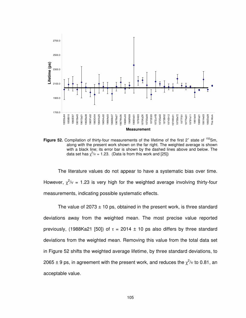
105
1700.0
1900.0
2100.0
2300.0
2500.0
2700.0
1955
Su6
4
1959
Bi1
0
1960
El0
7
1961
Be4
3
1961
Sa2
1
1962
Ba3
8
1963
Fo0
2
1963
Gr0
4
1964
Ho2
5
1965
Hu0
2
1966
As0
3
1966
Mc0
7
1967
Ba2
7
1967
Wo0
6
1968
Ku0
3
1968
Ri0
9
1968
Ve0
1
1970
Hi0
3
1970
KaZ
K
1970
Sa0
9
1972
El2
0
1972
LeY
B
1972
Sa4
2
1973
Br0
2
1974
Sh1
2
1974
Wo0
1
1975
Ba7
2
1977
Fi0
1
1977
Na0
1
1978
Ya1
1
1981
Is04
1988
Ka2
1
1991
He0
3
1992
De2
9
Thi
s W
ork
Measurement
Lif
eti
me (
ps
)
Figure 52. Compilation of thirty-four measurements of the lifetime of the first 2+ state of 152Sm,
along with the present work shown on the far right. The weighted average is shown with a black line; its error bar is shown by the dashed lines above and below. The data set has χ2/ν = 1.23. (Data is from this work and [25])
The literature values do not appear to have a systematic bias over time.
However, χ2/ν = 1.23 is very high for the weighted average involving thirty-four
measurements, indicating possible systematic effects.
The value of 2073 ± 10 ps, obtained in the present work, is three standard
deviations away from the weighted mean. The most precise value reported
previously, (1988Ka21 [50]) of τ = 2014 ± 10 ps also differs by three standard
deviations from the weighted mean. Removing this value from the total data set
in Figure 52 shifts the weighted average lifetime, by three standard deviations, to
2065 ± 9 ps, in agreement with the present work, and reduces the χ2/ν to 0.81, an
acceptable value.

106
After combining the present value with all previous measurements the
weighted average becomes 2052 ± 6 ps (χ2/ν = 1.38); omitting “1988Ka21” yields
a new weighted average of 2068 ± 7 ps (χ2/ν = 0.79), shown in Fig. 53.
1700.0
1900.0
2100.0
2300.0
2500.0
2700.0
1955
Su6
4
1959
Bi1
0
1960
El0
7
1961
Be4
3
1961
Sa2
1
1962
Ba3
8
1963
Fo0
2
1963
Gr0
4
1964
Ho2
5
1965
Hu0
2
1966
As0
3
1966
Mc0
7
1967
Ba2
7
1967
Wo0
6
1968
Ku0
3
1968
Ri0
9
1968
Ve0
1
1970
Hi0
3
1970
KaZ
K
1970
Sa0
9
1972
El2
0
1972
LeY
B
1972
Sa4
2
1973
Br0
2
1974
Sh1
2
1974
Wo0
1
1975
Ba7
2
1977
Fi0
1
1977
Na0
1
1978
Ya1
1
1981
Is04
1991
He0
3
1992
De2
9
Thi
s W
ork
Measurement
Lif
eti
me
(p
s)
Figure 53. Compilation of thirty-four measurements of the lifetime of the first 2+ state of 152Sm,
including the present work and omitting the value of 1988Ka21. The weighted average lifetime is shown with a black line; its error bar is shown by the dashed lines above and below. The data set has χ2/ν = 0.79. (Data is from this work and [25])
3.4.5.1 Delayed-Coincidence Method
The delayed-coincidence technique subset (including the present work),
yields a weighted average lifetime of 2041 ± 7 ps with χ2/ν = 1.86 (Fig. 54). If the
work labelled “1988Ka21” is omitted, the resulting new weighted average lifetime
is 2061 ± 9 ps, with χ2/ν = 0.97.

107
1800.0
1850.0
1900.0
1950.0
2000.0
2050.0
2100.0
2150.0
2200.0
2250.0
2300.0
1955
Su64
1962
Ba38
1963
Fo02
1965
Hu02
1966
Mc0
7
1967
Ba27
1968
Ku03
1968
Ri09
1972
El20
1981
Is04
1988
Ka21
1991
He03
1992
De29
This W
ork
Measurement
Lif
eti
me (
ps)
Figure 54. Compilation of thirteen delayed-coincidence measurements of the lifetime of the first
2+ state of 152Sm, along with the present work shown on the far right. The weighted average lifetime is shown with a black line; its error bar is shown by the dashed lines above and below. The data set has χ2/ν = 1.86. (Data is from this work and [25])
3.4.5.2 Coulomb Excitation Method
The Coulomb excitation measurements show a clear divergence from the
weighted average of the delayed coincidence measurements. The weighted
average lifetime from all the Coulomb excitation results (Figure 55) was
calculated to be 2088 ± 15 ps (χ2/ν = 0.49). These lifetime values were converted
by the evaluators from B(E2) values utilizing the formulas in equation 19,
modified to account for internal conversion:
( )5
10
2)2(
10156.81
γ
αττEEB
E ↓
×=+=
−
(35).

108
Raman et al use a theoretically calculated value αtotal = 1.141 to convert
the experimental B(E2) values into associated lifetimes. The experimental αtotal =
1.145 ± 0.029 [1].
1500.0
1700.0
1900.0
2100.0
2300.0
2500.0
2700.0
2900.0
1958
Sh01
1959
Bi10
1960
El07
1961
Be43
1961
Sa21
1963
Gr04
1964
Ho25
1967
Wo0
6
1968
Ve01
1970
KaZK
1970
Sa09
1972
Sa42
1973
Br02
1974
Sh12
1974
Wo0
1
1977
Fi01
This W
ork
Measurement
Lif
eti
me (
ps)
Figure 55. Compilation of sixteen Coulomb excitation measurements of the lifetime of the first 2+
state of 152Sm, along with the present work shown on the far right. The weighted average lifetime is shown with a black line; its error bar is shown by the dashed lines above and below. The data set has χ2/ν = 0.49. (Data is from this work and [25])
3.4.5.3 Comparing the Delayed-Coincidence and Coulomb Excitation Results
Statistical tests can be used to determine whether the Coulomb excitation
and delayed-coincidence methods are, in fact, different enough to be statistically
significant. Calculating a weighted average of τdel.coin. = 2041 ± 9 ps and τCoulex =
2088 ± 15 ps yields 2054 ± 21 ps with χ2/ν = 7.30 (one degree of freedom). A
comparison to a standard χ2 table of values indicates that the probability of the χ2
value being greater than this is 0.5%, and there is a statistically significant

109
systematic difference between the two methods. This also indicates that the
quoted uncertainty of the data set in Fig. 52 should be increased to ±21 ps.
If the 1988 work is removed, τdel.coin = 2061 ± 11 ps. The weighted average
of these two averages is 2068 ± 12 ps, with χ2/ν reduced to 2.43. This result still
indicates a statistically significant systematic difference between the measured
values obtained by the two techniques, increasing the uncertainty in the weighted
mean calculated for the entire data set of Fig. 53 to ±12 ps from ±7 ps.
One possible source of this discrepancy between the weighted mean
values obtained by the two techniques arises from the present experimental
uncertainty in the internal conversion coefficient required to convert a B(E2) into
a lifetime, as noted in Section 3.4.5.2.
Some remarks should also be made about the work by Karle et al in 1988
[50], as their experimental value is of the same precision as the present work but
differs by six standard deviations. This experiment involved two BaF2 detectors
using cylindrical large-volume high-efficiency crystals of 9 cm diameter and 9 cm
height. They tested their prompt coincidence width and obtained 375 ps FWHM
using a 60Co source. A 152Eu source was then used to re-measure the lifetime of
the 122 keV transition in 152Sm.
Karle et al measured the lifetime both via deconvolution of the prompt
detector response from the delayed curve (τ = 2017 ± 8 ps), and by measuring
the slope of the delayed portion of the time spectrum (τ = 2010 ± 9 ps). Raman et
al have weighted these two values to obtain τavg = 2014 ± 10 ps.

110
The energy gating technique employed to obtain these lifetime values
involved gating the 122 keV transition and a region about 1.32 MeV; however,
the structures of 152Sm and 152Gd (Fig. 33 and Ref. [1]) do not show any
transition of appreciable intensity in that energy range. An attempt to replicate
this energy gating method using the experimental data from this work yielded
very poor statistics. It is likely that a typographical error was made in Ref. [50]
regarding the energy gating regions.
In addition, the method by which the 152Eu source was prepared for the
work by Karle et al is not given; there is no adjustment indicated for the presence
of 154Eu in the sample. As established in Section 3.4.3, the presence of this
contaminant will affect half-life measurements and can be quantified. Therefore,
neglecting the presence of 154Eu in Ref. [50] would be one possible reason for a
lower reported lifetime value.
3.4.6 Other Properties of 152Sm
From the half-life measurement of 1437 ± 7 ps (τ = 2073 ± 10 ps) obtained
in this work, it is possible, as explained in Section 1.5, to obtain the B(E2)
associated with the 121.8 keV transition, and thereby the magnitude of the
quadrupole deformation, given a partial lifetime:
5
2
1010156.8)2(
γτ EEB
E
−×↓= (36).
Conversion of the measured lifetime into a partial lifetime [25] requires the
experimentally obtained internal conversion coefficient, αE2 = 1.145 ± 0.029 [1]:

111
( ) ( ) psE 1124447145.11207312 ±=+=+= αττ (37).
This results in the B(E2):
2242 0174.06846.01746846)2( befmeEB ±=±↓= (38).
In terms of Weisskopf units, the B(E2)↓ is 142.2 ± 3.6 W.u., indicating that
the transition 2+ � 0+ is of a collective nature.
In order to correctly express the quadrupole moment in units consistent
with formulas that relate this deformation to the dimensionless parameter β
(Section 1.5 and [2]), the unit e2 from the B(E2) will be accounted for when
converting this electric quadrupole moment:
eb 0.155.83)02;2(16 ±=→×= ++EBeQo π (39).
This is a magnitude only; the sign of the quadrupole moment cannot be
determined solely from the lifetime.

112
CHAPTER 4: CONCLUSION
4.1 Summary of Results
The DANTE BaF2 detector array has been characterized with an average
energy resolution of 10.5% at 662 keV, which did not change appreciably when
the detectors were mounted in the 8π array. Intrinsic prompt timing peak FWHMs
averaged 199 ps, which increased to an average of 270 ps after mounting the
detectors into the 8π.
The detector array has been shown to be capable of measuring half-lives
of nuclear excited states reliably in the nanosecond range, with multiple detectors
improving the statistical precision of such measurements over previous work.
This is evidenced by the re-measurement of the half-life of the first 2+ excited
state of 152Sm, having a transition energy of 121.8 keV, at t½ of 1437 ± 7 ps,
being more precise and in good agreement with all previous measurements
except one of equal precision.
Further, the combination of the HPGe detectors and BaF2 detectors at the
8π array has already proven of value in utilizing the superior energy resolution of
HPGe detectors to ascertain the presence of contamination in a 152Eu source,
and thus quantitatively determine if that contamination will have an effect on
measurements. By extension, in-beam experiments involving isobaric
contaminants can be treated similarly if necessary.

113
The DANTE array, as of this writing, is suitable for use in a nanosecond-
level half-life measurement for any state populated by a beta-decaying isotope
capable of being produced at TRIUMF-ISAC.
4.2 Further Directions
4.2.1 Gamma Backscattering Elimination
The presence of high-Z materials such as Heavimet, BGO, Barium and
Lead in the 8π array has the undesirable side effect of causing a high degree of
gamma ray scattering in the array. This affects timing peaks because there is a
finite time difference between gamma rays correlated by multiple scattering
events. These show up as extra peaks shifted away from the true prompt peak
when using a 60Co source. Previous workers have observed the problem as well
even when using only two BaF2 detectors [51]. A sample time spectrum
containing these backscattering events is shown in Figure 56(a) from the
detector pair 1 and 4, which are situated 120 degrees from each other.
Detectors situated 120 degrees from one another exhibited backscattering
events in their prompt timing peaks; the physical placement of the detectors
shown in Fig. 39 thus becomes of importance when understanding how to
eliminate this effect, which has been done by moving the detectors slightly further
away from the target chamber. This shields DANTE detectors from each other
since the intervening material is Heavimet and BGO. This was found to greatly
reduce the effect of scattering events on prompt or quasiprompt events, as
shown by the same detector pair in Figure 56(b).

114
(a)
(b)
Figure 56. Time spectra from the coincidence pair of detectors #1 and #4 (located 120 degrees from each other) when using a 60Co source. (a) Backscattering is present as indicated by the peak to the right of the true prompt peak. (b) Backscattering is essentially completely reduced by moving the detectors ~1 cm further away from the target chamber.
Measuring the half-life of the 366 keV state in 152Sm was not possible in
the present work because these backscattering events significantly affected the
shape of the delayed portion of the time spectrum after applying energy gates in
a similar way to the extraction of time spectra for the decay of the 122 keV state.
Both the application of exponential fit and the centroid shift methods to this
lifetime measurement are affected as both require the peaks to be skewed
Gaussians. In addition, the TACs, being set at 100 ns, were not optimized for
such short lifetimes.
4.2.2 Centroid-Shift Measurements
The change in the arrangement of the BaF2 detectors should lead to more
accurate lifetime measurements using the DANTE array, in particular at the few-
picosecond level in which the centroid-shift technique must be used. The
essentials of this technique are based on the fact that the introduction of a

115
lifetime into a gamma transition introduces a broadening of the timing signal in an
asymmetric fashion. This shifts the centroid of the detected timing peak relative
to a true prompt peak.
There are several ways to ascertain the true prompt peak characteristics;
one way is to use a 60Co source, but care must be taken to account for the
energy-dependent broadening effect in a prompt timing peak. Another method is
to use Compton continuum regions in the gamma spectra of interest to determine
prompt gamma-ray behavior.
To first order, fitting the prompt and shifted peaks with skewed Gaussians
will show a difference in the centroids and subtracting the two yields the half-life
of the excited state of interest. In practice there are other contributions that must
be taken into account, as noted in the detailed analysis undertaken by Seo [51],
and as established by Mach et al [52] which notes the energy dependence of the
prompt FWHM in timing analysis.
4.2.3 Use of the Full Array
Since the experiment which formed the basis of this thesis was carried
out, the FIFO and Ortec CO4020 logic modules have been fully-instrumented to
use all ten BaF2 detectors in the DANTE array. Since an array of four detectors
has already shown a notable improvement in the statistical precision of excited-
state half-life measurements, the full array of ten detectors would further enhance
this to the point where statistical errors would become negligible and the TAC
calibration uncertainty (a systematic error) would dominate. In the present work a

116
comparison of the statistical and systematic errors shows that the statistical
uncertainty of ±6 ps is greater than the systematic uncertainty of ±2 ps by a
factor of three.
To first order, the decrease in statistical error is calculated by the ratio of
the square root of the number of unique combinations of detectors. Thus, for ten
detectors, there are ninety unique combinations for ten detectors as compared to
twelve for four detectors, which yields an approximate factor of threen.
Assuming that the same source as used in this work was used with the
fully operational DANTE array, the statistical error would have been
approximately ±2 ps as opposed to ±6 ps. This promising improvement will
certainly motivate future experiments involving other radioactive isotopes whose
daughters have excited states with half-lives in the picosecond to nanosecond
range, and also shows that the systematic errors will tend to dominate in data
from DANTE when high-rate experiments are conducted.
4.2.4 HPGe Energy Gating
While the concept was discussed of HPGe detectors being used to gate
triple coincidences, this technique was not employed in the analysis which
formed the body of this work, owing to poor statistics when attempted.
An experiment involving a stronger (~500 kBq) isotopically pure 152Eu
source is planned for August 2009 by W. D. Kulp et al to measure intensities of
E0 transitions in 152Sm at the 8π. Because DANTE will be usable in addition to
n To be more precise, the exact calculation is (90 / 12)½ = 2.739.

117
PACES, and given the potential for high statistics in this experiment, it will be
possible to not only confirm the analysis thus far, but improve upon it in several
ways:
1. The presence of 154Eu will be of comparable magnitude and can be
more accurately assayed.
2. Improvement of the statistics in the data from BaF2-BaF2 coincidences,
as well as HPGe-BaF2-BaF2 coincidences.
3. The application of an energy gate on triple coincidences of HPGe-BaF2-
BaF2 will remove the sizable Compton contribution to the measurement of half-
lives.
4. The centroid shift measurement of the half-life of the 366 keV state will
be feasible.

118
APPENDIX 1
Supplementary equations from [8] for partial decay rates (λ) in s-1, partial
lifetimes (τ) in seconds, partial widths (Γ) in eV, downward transition
probabilities (B(EL)) in e2-fm2L where e is the fundamental unit of charge,
(B(ML)) in µN2-fm2L-2 where µN is the nuclear magneton, and the squares of
matrix elements (|M(EL/ML)|2) in Weisskopf units (W.u), incorporating Eγ in
MeV and A as the dimensionless mass number of the nucleus being
studied.
15
3/232
16
3
16
1 10754.9
)1(
10287.6
)1(
10582.6
)1(1)1(
−−− ×=
×
↓=
×
Γ==
AEEMEEBEE
E
γγ
τλ
8
3/452
10
5
16
2 10374.1
)2(
10156.8
)2(
10582.6
)2(1)2(
−−− ×=
×
↓=
×
Γ==
AEEMEEBEE
E
γγ
τλ
2
272
3
7
16
3 10947.2
)3(
10751.1
)3(
10582.6
)3(1)3(
−−− ×=
×
↓=
×
Γ==
AEEMEEBEE
E
γγ
τλ
14
32
14
3
16
1 10181.3
)1(
10697.5
)1(
10582.6
)1(1)1(
−−− ×=
×
↓=
×
Γ== γγ
τλ
EMMEMBMM
M
8
3/252
8
5
16
2 10479.4
)2(
10391.7
)2(
10582.6
)2(1)2(
−−− ×=
×
↓=
×
Γ==
AEMMEMBMM
M
γγ
τλ
2
3/472
1
7
16
3 10612.9
)3(
10586.1
)3(
10582.6
)3(1)3(
−−− ×=
×
↓=
×
Γ==
AEMMEMBMM
M
γγ
τλ

119
APPENDIX 2
I was involved in all stages of the construction and testing of the BaF2
detectors under laboratory conditions and after integrating them into the
8π array; with primary responsibility for data acquisition and analysis.
In addition, I acquired the absorption spectra to determine the properties
of the optical gels used to couple BaF2 crystals to the photomultiplier
tubes. These spectra verified the importance of transmitting the fast
component of the ultraviolet emission wavelengths of BaF2 to optimize
timing resolution.
Finally, I independently re-analyzed the lifetimes compiled by Raman et al.
and have identified some sources for the discrepancies observed in the
Coulomb Excitation method of obtaining lifetimes compared to those
obtained by the fast-timing delayed coincidence method.

120
REFERENCE LIST
[1] A. Artna-Cohen, Nuclear Data Sheets 79, 1 (1996).
[2] K. S. Krane, Introductory Nuclear Physics, edited by D. Halliday (Wiley, New
York, 1987), p. 845.
[3] M. Goeppert Mayer, Phys. Rev. 75, 1969 (1949).
[4] A. Bohr and B. Mottelson, Nuclear Structure (Volume II) (W. A. Benjamin, Inc.,
Don Mills, Ontario, Canada, 1975), p. 748.
[5] D. D. Frenne and E. Jacobs, Nuclear Data Sheets 79, 639 (1996).
[6] E. Browne and H. Junde, Nuclear Data Sheets 87, 15 (1999).
[7] W. D. Kulp et al, Phys. Rev. C 76, 034319 (2007).
[8] M. Baranger and E. Vogt, Advances in Nuclear Physics (Kluwer Academic
Publishers, 1977), 11.
[9] F. Villars, Annu. Rev. Nucl. Sci. 7, 185 (1957).
[10] D. R. Inglis, Phys. Rev. 97, 701 (1955).
[11] I. Hamamoto and B. Mottelson, Phys. Rev. C 79, 034317 (2009).

121
[12] G. F. Knoll, Radiation Detection and Measurement (Wiley, New York, 2000),
p. 802.
[13] W. D. Ehmann and D. E. Vance, Radiochemistry and Nuclear Methods of
Analysis, edited by D. E. Vance (Wiley, New York, 1991), p. 531.
[14] G. Grinyer, High-Precision Half-life Measurements for Superallowed Fermi β
Decays (University of Guelph, 2008).
[15] Stephen Derenzo, Martin Boswell, Marvin Weber and Kathleen Brennan.
Scintillation Properties. <http://scintillator.lbl.gov/> Accessed 02/01 2009.
[16] EG&G Ortec, Experiments in Nuclear Science (EG&G Ortec, 1987).
[17] Yale University. Recoil Distance Method.
<http://wnsl.physics.yale.edu/structure/equipment/rdm.html> Accessed 04/09
2009.
[18] T. K. Alexander and K. W. Allen, Can. J. Phys. 43, 9, 1563 (1965).
[19] N. Galinski, "Lifetime Measurement of the 6.79 MeV State in 15O" in Winter
Nuclear and Particle Physics Conference, Banff, Alberta, Canada, 13 Feb 2009.
[20] S. Mythili et al, Phys. Rev. C 77, 3, 035803 (2008).
[21] M. Laval, M. Moszyński, R. Allemand, E. Cormoreche, P. Guinet, R. Odru,
and J. Vacher, Nucl Instr Meth A 206, 169 (1983).

122
[22] H. Mach, R. L. Gill, and M. Moszyński, Nucl Instr Meth A 280, 1, 49 (1989).
[23] M. Moszyński and H. Mach, Nucl Instr Meth A 277, 2-3, 407 (1989).
[24] A. W. Sunyar, Phys. Rev. 98, 3, 653 (1955).
[25] S. Raman, C. W. Nestor Jr., and P. Tikkanen, Atomic Data and Nuclear Data
Tables 78 (2001).
[26] J. Äystö, Nuclear Physics A 805, 1-4, 162c (2008).
[27] P. E. Garrett et al, Nucl Instr Meth B 261, 1-2 (2007).
[28] G. C. Ball et al, J. Phys. G: Nucl. Part. Phys. 31, S1491 (2005).
[29] P. E. Garrett et al, Acta Phys. Pol. B 38, 1169 (2007).
[30] P. Dorenbos, Nucl Instr Meth A 486, 1-2, 208 (2002).
[31] S. J. Williams et al, J. Phys. G: Nucl. Part. Phys. 31, S1979 (2005).
[32] M. Moszyński, M. Kapusta, D. Wolski, M. Balcerzyk, S. O. Flyckt, P.
Lavoute, C. Marmonier, and H. Mach, IEEE Transactions on Nuclear Science 51,
4 (2004).
[33] S. J. Williams (private communication).
[34] Y. A. Valbis, Z. A. Rachko, and Y. L. Yansons, JETP Lett. 42, 4, 172-174
(1985).

123
[35] Photonis Imaging Sensors, Photomultiplier tubes product specification:
XP2020/URQ.
[36] D. C. Radford, computer code gf3, available from
http://radware.phy.ornl.gov/info.html. .
[37] S. Ritt, computer code MIDAS, available from http://midas.psi.ch/download. .
[38] Argonne National Labs, computer code EPICS, available from
http://www.aps.anl.gov/epics/. .
[39] M. Caprio, computer code gf3m, available from
http://wnsl.physics.yale.edu.proxy.lib.sfu.ca/cscan. .
[40] G. Grinyer, High-Precision Measurements of 26Na Beta Decay (University of
Guelph, 2004).
[41] P. Finlay, High-Precision Branching Ratio Measurement for the
Superallowed Beta Emitter 62Ga (University of Guelph, 2007).
[42] M. Trinczek, Limits on Heavy Neutrino Mixing from the Beta Decay of 38mK
Confined in a Magneto-Optical Trap (Simon Fraser University, 2001).
[43] D. W. Marquardt, SIAM J. Appl. Math. 11, 2, 431 (1963).
[44] C. Amsler et al, Physics Letters B 667, 1 (2008).
[45] P. Belli et al, Nucl Instr Meth A 572, 2, 734 (2007).

124
[46] V. D. Risovany, A. V. Zakharov, E. P. Klochkov, T. M. Guseva, V. B.
Ponomarenko, and V. M. Chernyshov, "Production of Gamma-Sources, Based
on Europium Oxide in Fast Reactors" in IAEA-TECDOC--884: Absorber
materials, control rods and designs of shutdown systems for advanced liquid
metal fast reactors, Vienna, Austria, 3-7 Jul 1995, p. 205.
[47] C. W. Reich and R. G. Helme, Nuclear Data Sheets 85, 171 (1998).
[48] K. G. Leach, High-Precision Measurement of the Superallowed Beta Decay
Branching Ratio of 38mK (University of Guelph, 2008).
[49] M. Hellström, H. Mach, B. Fogelberg, D. Jerrestam, and L. Spanier, Phys.
Rev. C 43, 3, 1462 (1991).
[50] W. Karle, M. Knopp, and K.-H. Speidel, Nucl Instr Meth A 271, 3, 507 (1988).
[51] T. Seo, Nucl Instr Meth A 325, 1-2, 176 (1993).
[52] H. Mach et al, Phys. Rev. Lett. 63, 143 (1989).
[53] R. S. Hager and E. C. Seltzer, Nucl. Data Tables A4, 1 (1968).
[54] I. M. Band, M. B. Trzhaskovskaya, C. W. Nestor Jr., P. O. Tikkanen, and S.
Raman, At. Data Nucl. Data Tables 81, 1-2 (2002).


![· 2019. 6. 11. · Chlorine (as C12) (ppm) TTHMs [Total Trihalomethanes] (ppb) Barium (ppm) Fluoride (ppm) Nitrate [measured as Nitrogen] (ppm) Tetrachloroethylene (ppb) Water additive](https://img.pdfslide.net/doc/110x75/5fc23e762fd1747c672d7828/2019-6-11-chlorine-as-c12-ppm-tthms-total-trihalomethanes-ppb-barium.jpg)


![Index [ftp.feq.ufu.br]ftp.feq.ufu.br/Luis_Claudio/Segurança/Safety/Double/fire_handbook... · Backdraft Explosion 174 Barium 216 Barium Carbonate 300 Barium Chlorate 300 Barium Nitrate](https://img.pdfslide.net/doc/110x75/5ea2585052451660ed3ed304/index-ftpfequfubrftpfequfubrluisclaudioseguranasafetydoublefirehandbook.jpg)