Building Dynamic simulation uncertainty evaluation based

Building Dynamic simulation uncertainty evaluation based on

sensitivity analysis

Loïc Walrave

Thesis to obtain the Master of Science Degree in

Energy Engineering and Management

Supervisors: Prof. Carlos Augusto Santos Silva

Eng. Matthieu Caille

Examination Committee

Chairperson: Prof. Jorge de Saldanha Gonçalves Matos

Supervisor: Prof. Carlos Augusto Santos Silva

Member of the Committee: Dr. Rui Pedro da Costa Neto

November 2017

Page 2 of 50

Acknowledgment

My deepest gratitude goes to my supervisor Carlos Augusto Santos Silva, for according me time and support

throughout this Master Thesis and for proof reading my report. I would also like to thank him for his guidance

and good advice that helped me write this report.

I would like to thank the whole SES team for the warm welcome and their availability. By making me part of

the team, they allowed me to work in a great and friendly environment.

Finally, I want to express my gratitude to Matthieu Caille, my manager at Synergy Efficiency Solutions,

allowing me to work and to learn in the best conditions.

Page 3 of 50

Table of contents

Acknowledgment ........................................................................................................................................... 2

Table of contents ........................................................................................................................................... 3

List of tables................................................................................................................................................... 5

List of figures ................................................................................................................................................. 5

Acronyms ....................................................................................................................................................... 6

Abstract .......................................................................................................................................................... 7

I. Introduction ............................................................................................................................................ 8

1. Context and motivation .................................................................................................................. 8

2. Problem formulation ...................................................................................................................... 9

3. Objective of the research ............................................................................................................... 9

4. Research question ....................................................................................................................... 10

5. Structure of the thesis .................................................................................................................. 10

II. Literature review .................................................................................................................................. 11

1. Building simulations ..................................................................................................................... 11

2. Uncertainty in simulations ............................................................................................................ 12

3. Sensitivity analysis....................................................................................................................... 14

III. Case Study ...................................................................................................................................... 18

1. KMT overviews ............................................................................................................................ 18

2. KMT Simulation details ................................................................................................................ 19

3. Simulation results of non-calibrated simulation ........................................................................... 21

4. Comparison of data measured and simulation ............................................................................ 23

IV. Methodology .................................................................................................................................... 31

1. KMT work plan of measurement .................................................................................................. 31

2. Software used .............................................................................................................................. 32

3. Methodology to perform the sensitivity analysis .......................................................................... 33

Page 4 of 50

V. Results ................................................................................................................................................. 39

1. Overview of PEAR, SRC and PCC results .................................................................................. 39

2. Detailed results ............................................................................................................................ 40

VI. Discussion ....................................................................................................................................... 46

VII. Conclusions ..................................................................................................................................... 48

VIII. References ...................................................................................................................................... 49

Page 5 of 50

List of tables

Table 1: Selected design (input) parameters studied by Nguyen and Reiter .............................................. 15

Table 2: Selected design (input) parameters studied by Song, Wei, Sun and Tian .................................... 16

Table 3: Selected design (input) parameters studied by Solmaz, Halicioglu and Gunhan ......................... 16

Table 4: Performance data of the window glass material ........................................................................... 20

Table 5: Envelope materials properties ....................................................................................................... 21

Table 6: Results of the initial simulation - Main chiller design size reference capacity ............................... 21

Table 7: Results of the initial simulation - Main cooling tower fan power at design air flow rate ................ 22

Table 8: Results of the initial simulation - Pumps and fans electricity end uses ......................................... 22

Table 9: MBE and CV(RMSE) of the weather file used for the simulation .................................................. 25

Table 10: MBE and CV(RMSE) of the simulation results of the sun-exposed room ................................... 29

Table 11: MBE and CV(RMSE) of the simulation results of the sun-protected room ................................. 29

Table 12: List of the parameters studied in the SA ..................................................................................... 36

Table 13: List of the SA outputs .................................................................................................................. 37

Table 14: Example of an equipment input file ............................................................................................. 44

List of figures

Figure 1: Sources of uncertainties ............................................................................................................... 13

Figure 2: Overview of the Kompas Multimedia Tower ................................................................................ 18

Figure 3: SketchUp drawing of the Kompas Tower ..................................................................................... 19

Figure 4: Results of the initial simulation - Energy Use Intensity (EUI) ....................................................... 22

Figure 5: Results of the initial simulation - End Use Percentage (EUP) ..................................................... 23

Figure 6: Comparison of measured and simulated outside temperature .................................................... 24

Figure 7: Comparison of measured and simulated humidity ratio ............................................................... 24

Figure 8: Location of the two rooms used for the temperature and humidity measures at KMT ................ 26

Figure 9: Comparison of the measured data and the simulation results of the sun-exposed room ............ 27

Figure 10: Comparison of the measured data and the simulation results of the sun-protected room ........ 28

Figure 11: Data measurement in Kompas Multimedia Tower ..................................................................... 31

Figure 12: JEPlus - An EnergyPlus simulation manager for parametrics ................................................... 33

Figure 13: Process of the sensitivity analysis using JEPlus and SimLab ................................................... 34

Figure 14: Factor of impact of the variables on each output using the PEAR statistical analysis .............. 39

Figure 15: Factor of impact of the variables on each output using the PCC statistical analysis ................. 39

Figure 16: Factor of impact of the variables on each output using the SRC statistical analysis ................. 40

Figure 17: Results of the sensitivity indices of the parameters on each output using the PEAR method .. 42

Figure 18: Envelope construction input file ................................................................................................. 44

Figure 19: Absolute average sensitivity indices of each input parameters ................................................. 45

Page 6 of 50

Acronyms

ACH: Air Changes per Hour

FCU: Fan Coil Unit

HVAC: Heating, Ventilation and Air Conditioning

KMT: Kompas Multimedia Tower

LHS: Latin Hypercube Samplings

PCC: Partial Correlation Coefficient

PEAR: Pearson product moment correlation

SA: Sensitivity Analysis

SES: Synergy Efficiency Solutions

SRC: Standardized Regression

Page 7 of 50

Abstract

Building dynamic simulation are used to estimate the energy performance of buildings and to size some of

the equipment that will be used. It is a valuable tool to help designing sustainable buildings, by showing the

impact of different solutions on the building's behavior in both new buildings and retrofit projects.

However, models are by definition approximate and represent a simplification of the real physical world.

Sources of uncertainty abound in building simulation and must be taken into account into the results of the

simulations. These sources have been identified and classified in three categories: the simplification of the

model, the input parameters based on assumptions and standards values and the physical processes used

by the software. This work will study the impact of the input parameters in the results of the simulation.

Considering the uncertainty factors aims at improving designer confidence in the simulations.

Sensitivity analysis plays an important role in the understanding of complex models. It helps to identify the

influence of input parameters in relation to the outputs. For building energy models, combining sensitivity

analysis and simulations tools helps to rank the input parameters (or family of parameters) and then to select

the most appropriate to be considered.

This study aims to analyze and illustrate the potential usefulness of improving the accuracy of the input

parameters in order to reduce the models uncertainty.

The analysis of the results showed that the impact on the simulation’s results depends on the type of inputs.

It was found that some parameters that have a major influence on the outputs can be easily made more

precise such as the wall’s characteristics. Moreover some parameters that are complex to estimate can also

impact the accuracy of the results, such as the air infiltration rate through the building’s envelope.

‘’Solving our energy challenges is not about producing more, but finding better ways to use what is already

available’’ (US Department of Energy, 2016).

Keywords:

Dynamic Simulation, Sensitivity Analysis, Calibration, Uncertainty Optimization Scheme

Page 8 of 50

I. Introduction

1. Context and motivation

Energy consumption related to the building sector is recognized as a major part of the total energy

consumption worldwide with 31% of the final energy consumption in the EU in 2014 (Global Alliance for

Buildings and Construction, 2016) and consequently a significant source of greenhouse gas emissions. The

growth in population, building services and comfort levels guarantees that this tendency will continue in the

forthcoming years.

In order to reduce the global energy needs of buildings, it is possible to evaluate the impact of different

design solutions on the building’s behavior and expected energy consumption combining architecture and

engineering software. This approach is seen as a method that can deliver substantial gains in terms of

designing and assessing the environmental cost of buildings, necessary to achieve sustainable design.

Dynamic simulation are more and more used during the design process of making a new building to reach

more energy efficient buildings. For now, most architects do not use any tool asides from intuition or common

sense to estimate the impact of modifying building’s characteristics on its future energy consumption.

However, design and simulation software make it easier for architects and engineers to evaluate energy

performance of buildings at every stage in their life cycle and to help them design the systems that will be

installed.

Turning a 3D design into an energy model is made through a simplification of the authentic complex real

physical world involving thermal transfer, solar radiance, characteristics of materials, design, weather and

so on. The goal is to generate complete simulation models that will be used to project the actual operational

performance of the building in its environment and its expected use.

Many tools have been developed to model the energy consumption in buildings (EnergyPlus, TRNSYS,

ESP-r), especially to size the systems used for heating, cooling, ventilation and lighting. The models

produced take into account the coupling between phenomena (e.g. interactions between occupancy,

exterior conditions, envelope, HVAC, etc.) by using a large number of diverse input variables.

Page 9 of 50

2. Problem formulation

Developing building simulations at the project phase have usually little adherence to real energy

consumption when the building is operating. Sources of uncertainty abound in building simulation due to

simplification and assumptions made to draw the energy model. That is why the main impediment to

modeling are cost and doubts about usefulness. Hence it is essential to take into consideration the accuracy

of the model to know to what extent the results can be relied on, and to identify and reduce the sources of

uncertainty.

The uncertainties come from 3 levels: the simplification of the model, the input parameters based on

assumptions and standards values and the physical processes used by the software. It is very complicated

for the user to have an impact on the software physical model, but a lot of work can be done on the input

parameters. These parameters are taken from real data (material, design, measurement), assumptions

(time of use of the equipment, occupancy) and from collected data measured on-site or nearby (weather

files).

The uncertainty in these inputs parameters can be due to a lack of technical information about the building

and its systems and to assumptions that are difficult to make in the context of the project.

To partially solve this issue, standard values provided by the American Society of Heating, Refrigerating

and Air-Conditioning Engineers (ASHRAE) Guidelines are very often used. However, even if standard

values can be a good approximation, it is hard to know to what extend they approach the reality of each

buildings.

3. Objective of the research

A great way to determine which parameters influence the most the precision of the model is to perform a

sensitivity analysis which assess the relationship between variations in input parameters to variation in

output (predicted) parameters. All the design parameters do not affect building energy performance on the

same level. The impact on the model of these sensitive parameters will be measurable, therefore it will be

possible to ascertain whether the extra effort is necessary and worth to achieve better predictions. The

importance level of the parameters will guide the decision-making process and extract priority input

parameters that must be particularly accurate to improve the accuracy of the results.

This thesis aims at evaluate the sources of uncertainty of these simulation models using a sensitivity

analysis and to identify how these results can be used to improve the reliability further simulations.

Different methods are possible to perform a sensitivity analysis. Three of them will be realized to compare

their global results and one will be chosen to be applied to go more in details.

Page 10 of 50

4. Research question

To what extent do the assumptions made regarding the input parameters affect the predictions of the

simulation?

5. Structure of the thesis

Following the structure of the thesis, the first part is the literature review concerning the area of study. The

literature review seeks to provide a foundation for this research by establishing the current ‘‘state of the art’’

in the fields touched upon over the course of this research project, and how the outcomes of this project

could affect the future directions of these fields. It will be developed in three parts: To begin with, an overview

of the dynamic simulations in the buildings area will be made. It will be explained on what there are based

and what in what purposed they are realized. Then different papers dealing with the uncertainty in

simulations will be explained and address the question of the calibration of the models. The last part of the

literature review will treat the sensitivity analyses realized in the building area, giving an overview of the

sensitivity methods to use and the parameters that influenced the most the results of the simulations.

The second part of this work is the presentation of the case study: the dynamic simulation of the Kompas

Multimedia Tower (KMT) in Jakarta, Indonesia. This part will show the initial goal of the project and show

the details of the simulation realized for the project. On the purpose of this work, on-site measurements

were realized in this tower and a comparison of the data measured and the results of the initial simulation

will be drawn.

The third part will explain how the different software used in this study work and how they were combined.

Then, the choice of a sensitivity analysis method will be made and the different steps to perform it will be

detailed. This part will terminate with the choices made when designing the uncertainty optimization scheme.

The fourth part contains the results of the sensitivity analysis and highlights the parameters that influenced

the most the simulation. Taking into account the context of the simulation and of the project, these results

will help to understand how the simulation can be more accurate and used to help designing sustainable

buildings.

This part, as the last part of thesis, is dedicated to the discussion around this study. It is important to keep

these results in a specific context and to take a step back to see how the findings could be adapted to

different projects. In different contexts, other solutions can be put forward in order to reduce the uncertainty

of the simulations.

Page 11 of 50

II. Literature review

1. Building simulations

Assessing a future building or a retrofit project to its external condition and use is a great way to see the

improvements that can be made on its design, on the choice of the materials and on the choice of its

equipment. Dynamic thermal simulation models have a wide range of applications from simple regulatory

compliance calculations to advanced estimates of operational performance in large complex buildings.

Advanced modeling techniques can be used to accurately predict thermal performance in both new build

and retrofit projects; they can also be used to simulate day-lighting and complex air movement.

As explained by Brent Huchuk, William O’Brien and Cynthia A. Cruickshank, the increased availability and

capability of dynamic computer simulation techniques of a building's performance provide a possible

strategy for finding the ideal balance between the often-conflicting benefits from modern design and the

comfort of the occupants. (Huchuk, O’Brien, & Cruickshank, 2013)

In their paper ‘’ The Advantages of Building Simulation for Building Design’’, K.H. Beattie and I.C. Ward

explain that to better design the building and size its equipment, accurate information are required on the

magnitude, the duration and the time of occurrence of internal peak temperatures during the occupied period

and of heating and cooling loads variation over the season. It can help for example the building designer to

know if natural ventilation will work or if air conditioning is required. (Beattie & Ward, 2017) Better building

design means better in terms of environmental quality and energy consumption.

With dynamic simulation, you can guess the cause of an effect (even if measuring its impact is more or less

precise), for example peak of temperature occurs when the solar radiation is higher, or temperature drops

when the building is under the shade of another building, etc.

Also it offers interaction with real climate data considering hourly values for:

Dry Bulb T° and Wet bulb T°c

Direct and diffuse solar radiation

Wind speed and Wind direction

According to K.H. Beattie and I.C. Ward, there is a tendency to over-size the systems when too simple

calculations are made: ‘’ The consequences of over-sizing plant in terms of increased capital costs,

increased operating energy requirements and increased CO2 emissions to the environment should make

the building services engineer seek a better method for designing building. ’’

Page 12 of 50

The use of dynamic simulation allows more creativity by the building services engineer rather than

just concentrating on peak loads to make the plant big enough.

2. Uncertainty in simulations

A study made by K.H. Beattie and I.C. Ward shows that most architects in Ireland do not use any method

except from common sense or intuition to assess the impact of changing a building’s characteristics on its

future energy efficiency. (Beattie & Ward, 2017)

The two main inhibitions to modeling are cost and doubts about usefulness because of computing time and

uncertainty of the results

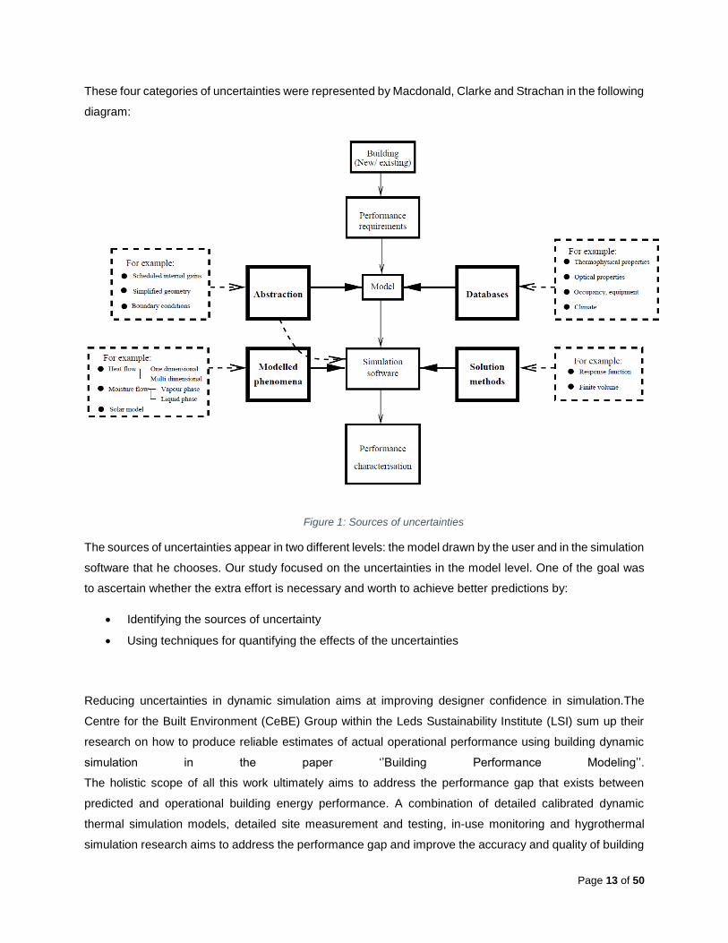
As shown in ‘’Assessing Uncertainty in Building Simulation’’ by Macdonald I.A., Clarke J.A. and Strachan

P.A., the sources of uncertainties can be organized in 4 categories:

Abstraction: While transferring the design to a computer representation: simplifications and

concessions have to be made (e.g. averaging the occupancy zone)

Databases: Information used doesn’t match the element to be modeled so assumptions have to be

made on properties or measurements realized previously.

Modeled phenomena: Physical processes modeled differently depending on the simulation

software.

Solution methods: There are various solution techniques available, generally causing a loss of

precision (e.g. in resorting to numerical discretization techniques a discretization error is introduced

to the solution)

(Macdonald, Clarke, & Strachan, 1999)

For the category “databases”, usually more information can be found at the expense of time and other

resources.

Page 13 of 50

These four categories of uncertainties were represented by Macdonald, Clarke and Strachan in the following

diagram:

The sources of uncertainties appear in two different levels: the model drawn by the user and in the simulation

software that he chooses. Our study focused on the uncertainties in the model level. One of the goal was

to ascertain whether the extra effort is necessary and worth to achieve better predictions by:

Identifying the sources of uncertainty

Using techniques for quantifying the effects of the uncertainties

Reducing uncertainties in dynamic simulation aims at improving designer confidence in simulation.The

Centre for the Built Environment (CeBE) Group within the Leds Sustainability Institute (LSI) sum up their

research on how to produce reliable estimates of actual operational performance using building dynamic

simulation in the paper ‘’Building Performance Modeling’’.

The holistic scope of all this work ultimately aims to address the performance gap that exists between

predicted and operational building energy performance. A combination of detailed calibrated dynamic

thermal simulation models, detailed site measurement and testing, in-use monitoring and hygrothermal

simulation research aims to address the performance gap and improve the accuracy and quality of building

Figure 1: Sources of uncertainties

Page 14 of 50

simulation, ultimately closing the loop between estimated and operational energy consumption (CeBe & LSI,

2015).

The prediction accuracy of building energy models has been examined by Mohammad Royapoor and Tony

Roskilly using energy monitoring. In their paper ‘’ Building model calibration using energy and environmental

data’’, they used a set of two calibrated environmental sensors together with a weather station and deployed

them in a 5 floor office building to examine the accuracy of an EnergyPlus virtual building model. Using

American Society of Heating, Refrigerating and Air-Conditioning Engineers (ASHRAE) Guide 14, the model

was calibrated to achieve Mean Bias Error (MBE) values within ±5% and Cumulative Variation of Root Mean

Square Error (CV(RMSE)) values below 10%. The calibrated EnergyPlus model was able to predict annual

hourly space air temperatures with an accuracy of ±1.5◦C for 99.5% and an accuracy of ±1◦C for 93.2% of

the time (Royapoor & Roskilly, 2015).

3. Sensitivity analysis

Sensitivity analysis helps to identify the influence of input parameters (e.g. wall insulation thickness) in

relation to the outputs (e.g. Total HVAC electric demand power). It can also be a tool to understand the

behavior of the model and can then facilitate its development stage.

In the field of building energy models, combining sensitivity analysis and simulation tools can be useful as

it helps to rank the input parameters (or family of parameters) and then to select the most appropriate to be

considered, depending on the objective of the modeling.

As detailed in ‘’Application of sensitivity analysis in building energy simulations’’, D. Garcia Sanchez, B.

Lacarrière, M. Musy and B. Bourges show that a solution consists of using a detailed model in the upstream

stage, combined with a sensitivity analysis in order to rank the set of parameters and identify the coupling

between them. Then, the selection of the most important variable helps to define the structure of the

simplified model (Sanchez, Lacarrière, Musy, & Bourges, 2014).

Anh-Tuan Nguyen and Sigrid Reiter demonstrate that sensitivity analysis in the early stages of the design

process can give important information about which design parameters to focus on in the next phases of

the design and “improve the efficiency of the design process and be very useful in an optimization of building

performance” (Nguyen & Reiter, 2015).

However, building energy models are generally computationally expensive. Therefore, there exists a

growing concern about the relevancy of a SA method for a building energy model and how reliable a method

is.

To choose which sensitivity analysis method to perform in this study, the results of several papers evaluating

the accuracy and the complexity of the different methods were put together:

Page 15 of 50

As the computationally cheapest method of all, the Morris method showed acceptable capability in

quantifying sensitivity and interaction among parameters, but it was not reliable in ranking variables

(Nguyen & Reiter, 2015)

Variance-based sensitivity indices (VBM) generally provide better information to distinguish non

linearities and interactions but the computational cost is much higher (Nguyen & Reiter, 2015)

The Pearson product moment correlation coefficients (PEAR), the PCC (Partial Correlation

Coefficient) and the SRC (Standardized Regression Coefficient) offered a great compromise

between accuracy and computational cost in building energy models. (Nguyen & Reiter, 2015)

Since there are many input parameters in every dynamic simulations, another important factor to perform

the sensitivity analysis is to know which parameters are relevant to analyze. It is noticeable that almost the

same parameters are analyzed in several studies.

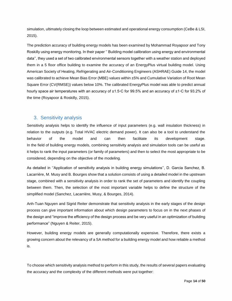
The following design parameters were studied by Anh-Tuan Nguyen and Sigrid Reiter:


Table 1: Selected design (input) parameters studied by Nguyen and Reiter

Page 16 of 50

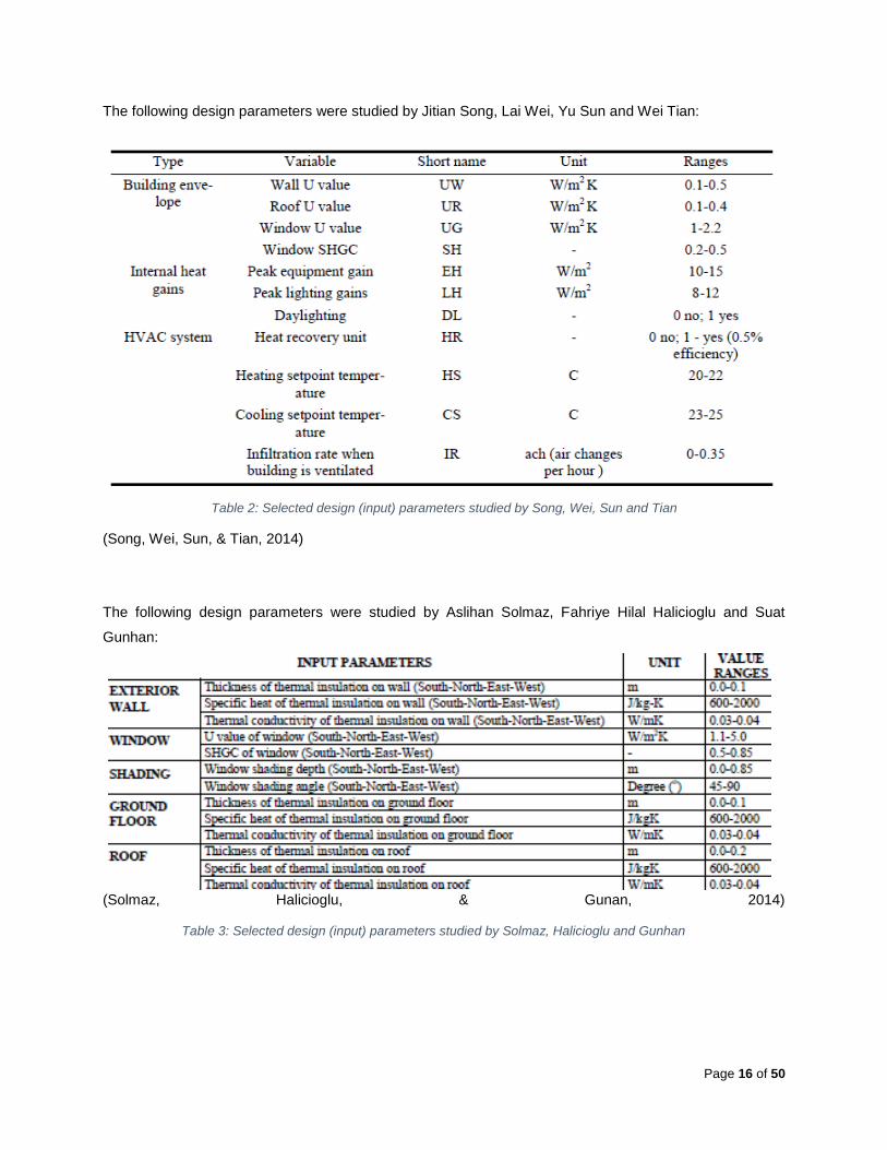
The following design parameters were studied by Jitian Song, Lai Wei, Yu Sun and Wei Tian:

(Song, Wei, Sun, & Tian, 2014)

The following design parameters were studied by Aslihan Solmaz, Fahriye Hilal Halicioglu and Suat

Gunhan:

(Solmaz, Halicioglu, & Gunan, 2014)

Table 2: Selected design (input) parameters studied by Song, Wei, Sun and Tian

Table 3: Selected design (input) parameters studied by Solmaz, Halicioglu and Gunhan

Page 17 of 50

8 parameters were selected for this work, carefully chosen according to the results of the previous papers:

P1: Windows overall heat transfer coefficient (U value) P2: Windows Solar Heat Gain Coefficient (SHGC) P3: Wall insulation thickness P4: Concrete density (the concrete is one of the layers of the walls) P5: Roof insulation thickness P6: Lights P7: Equipment P8: Air infiltration

When performing simulation for real projects, whether there are building retrofit or new building project, most

of the parameters are assumed with a certain range of precision. In fact, it is very difficult to know every

details of a construction. The schedules are also very imprecise, whether there are for the occupancy, the

lighting, the equipment etc.

This study particularly aims at evaluating the impact on the simulation of these uncertain parameters, based

on assumptions. It would allow to know which one have the most impact and in which a supplementary

study increasing their accuracy would improve significantly the model.

The goal is not to realize a study of the impact of different solutions such as implementing shading systems,

but it is to find how to improve the accuracy of building simulations by knowing which parameters have to

be more detailed.

Page 18 of 50

III. Case Study

1. KMT overviews

The building studied is the Kompas Multimedia Tower located in Jarkarta, Indonesia. Kompas is a company

that owns an important news channel in Indonesia. This tower is part of a complex of 3 towers that form the

headquarters of the company.

The building has 25 stories above ground level and 3 stories below ground level forming the parking lots. Each story was divided into several zones:

The basement consists of the parking area, the stairs and the ME room.

Floor 1: Consists of big studio, crew room, control and ME room, FOH room, Kompas TV room, meeting room, property room, waiting room, wardrobe room and service area.

Floor 2: Consists of Kompas Iklan room, FOH room, lobby, meeting room, middle studio, storage room, Camera room, core tower and service area (toilet, corridor, stairs and escalator).

Floor 3: Consists of audio control room, dimmer room, GM room, lobby, Kompas Iklan room, meeting room, panel room, core tower, production control room, storage room and service area (toilet, corridor, stairs, escalator).

Floor 4: Consists of AHU room, Kompas Redaksi room, library, lobby, core tower and service area (toilet, corridor, stairs and escalator).

Floor 5: Consists of Data Center, Kompas Redaksi Room, core tower, lobby, meeting room, and service area (toilet, corridor, stairs, and escalator).

Floor 6 and 7: Consist of Kompas TV room, core tower and service area (toilet, corridor, stairs, and escalator).

Floor 8 to 24: Consist of core tower and tenant area.

Floor 25: Consists of roof area and lift zone.

Figure 2: Overview of the Kompas Multimedia Tower

Page 19 of 50

2. KMT Simulation details

In the year 2014, the company Synergy Efficiency Solutions had been contracted by Kompas to analyze its

future building. A simulation work based on the architect’s drawings was carried out to assess the

performance of the design specified by the Mechanical, electrical, and plumbing (MEP) consultant.

Additionally, this simulation work also assessed the performance of the exterior facade, i.e. the combination

of glass type and the perforated panel that acts as the double skin of the building.

All the results of the simulation are taken from a report written by the company that was used for this work:

(Synergy Efficiency Solutions, 2015)

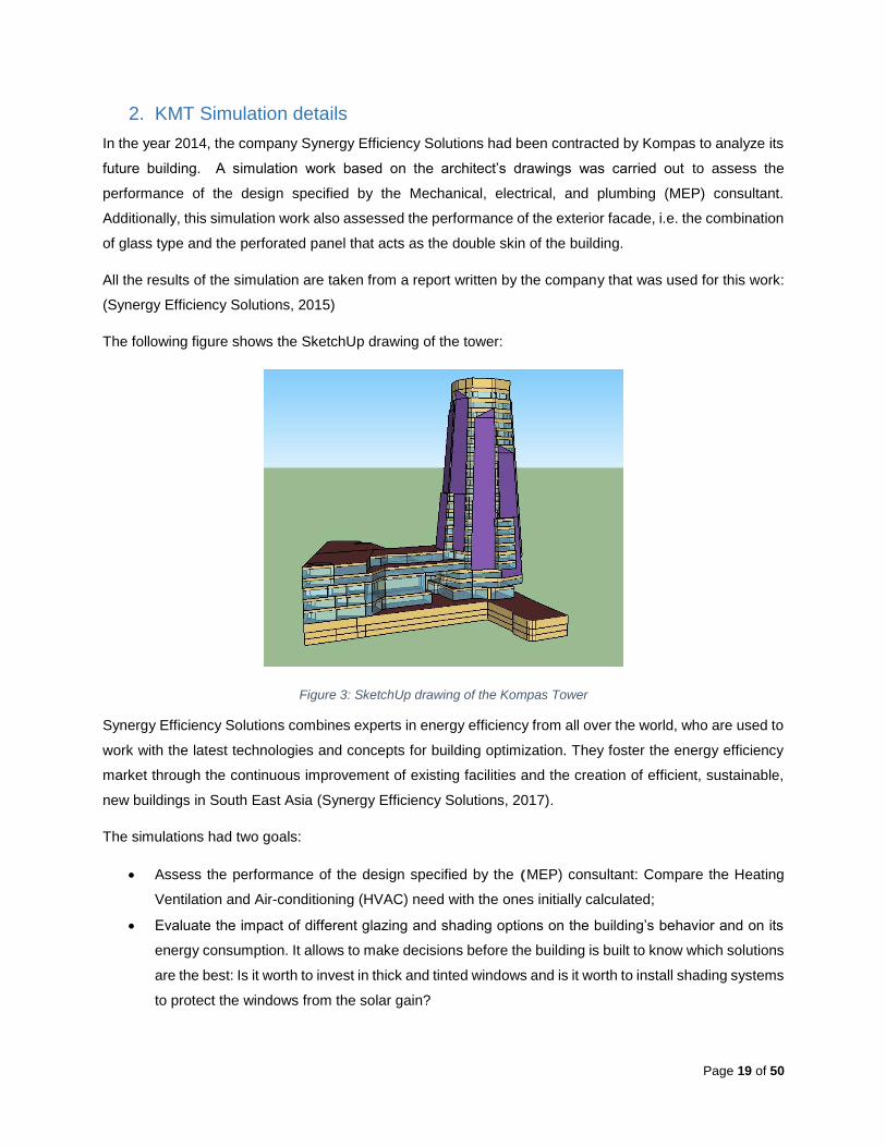
The following figure shows the SketchUp drawing of the tower:

Figure 3: SketchUp drawing of the Kompas Tower

Synergy Efficiency Solutions combines experts in energy efficiency from all over the world, who are used to

work with the latest technologies and concepts for building optimization. They foster the energy efficiency

market through the continuous improvement of existing facilities and the creation of efficient, sustainable,

new buildings in South East Asia (Synergy Efficiency Solutions, 2017).

The simulations had two goals:

Assess the performance of the design specified by the (MEP) consultant: Compare the Heating

Ventilation and Air-conditioning (HVAC) need with the ones initially calculated;

Evaluate the impact of different glazing and shading options on the building’s behavior and on its

energy consumption. It allows to make decisions before the building is built to know which solutions

are the best: Is it worth to invest in thick and tinted windows and is it worth to install shading systems

to protect the windows from the solar gain?

Page 20 of 50

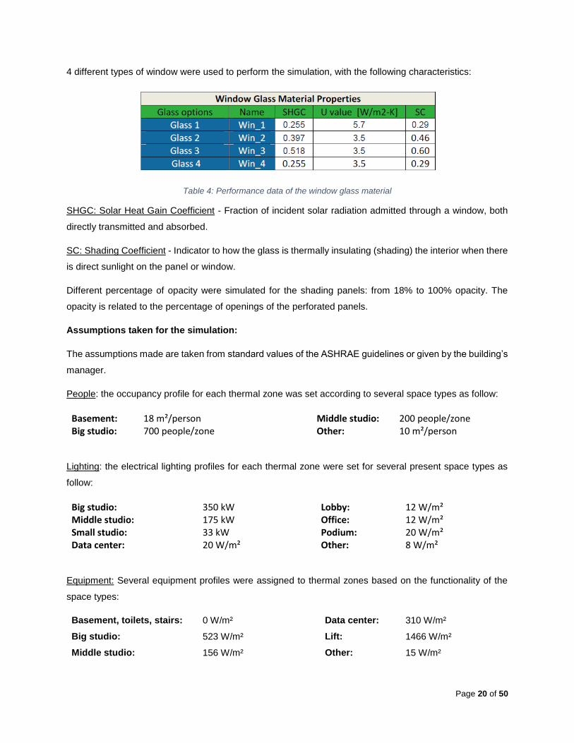
4 different types of window were used to perform the simulation, with the following characteristics:

Table 4: Performance data of the window glass material

SHGC: Solar Heat Gain Coefficient - Fraction of incident solar radiation admitted through a window, both

directly transmitted and absorbed.

SC: Shading Coefficient - Indicator to how the glass is thermally insulating (shading) the interior when there

is direct sunlight on the panel or window.

Different percentage of opacity were simulated for the shading panels: from 18% to 100% opacity. The

opacity is related to the percentage of openings of the perforated panels.

Assumptions taken for the simulation:

The assumptions made are taken from standard values of the ASHRAE guidelines or given by the building’s

manager.

People: the occupancy profile for each thermal zone was set according to several space types as follow:

Basement: 18 m²/person Middle studio: 200 people/zone Big studio: 700 people/zone Other: 10 m²/person

Lighting: the electrical lighting profiles for each thermal zone were set for several present space types as

follow:

Big studio: 350 kW Lobby: 12 W/m² Middle studio: 175 kW Office: 12 W/m² Small studio: 33 kW Podium: 20 W/m² Data center: 20 W/m² Other: 8 W/m²

Equipment: Several equipment profiles were assigned to thermal zones based on the functionality of the

space types:

Basement, toilets, stairs: 0 W/m² Data center: 310 W/m²

Big studio: 523 W/m² Lift: 1466 W/m²

Middle studio: 156 W/m² Other: 15 W/m²

Page 21 of 50

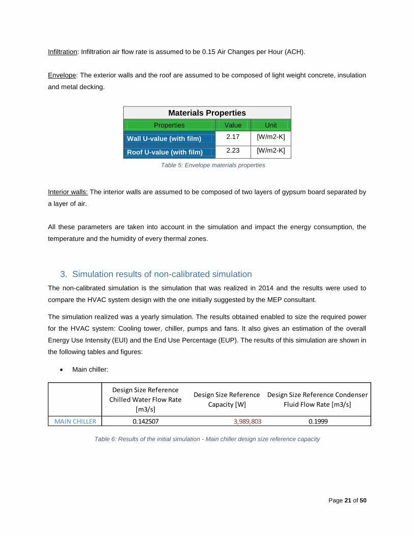
Infiltration: Infiltration air flow rate is assumed to be 0.15 Air Changes per Hour (ACH).

Envelope: The exterior walls and the roof are assumed to be composed of light weight concrete, insulation

and metal decking.

Interior walls: The interior walls are assumed to be composed of two layers of gypsum board separated by

a layer of air.

All these parameters are taken into account in the simulation and impact the energy consumption, the

temperature and the humidity of every thermal zones.

3. Simulation results of non-calibrated simulation

The non-calibrated simulation is the simulation that was realized in 2014 and the results were used to

compare the HVAC system design with the one initially suggested by the MEP consultant.

The simulation realized was a yearly simulation. The results obtained enabled to size the required power

for the HVAC system: Cooling tower, chiller, pumps and fans. It also gives an estimation of the overall

Energy Use Intensity (EUI) and the End Use Percentage (EUP). The results of this simulation are shown in

the following tables and figures:

Main chiller:

Table 6: Results of the initial simulation - Main chiller design size reference capacity

Design Size Reference

Chilled Water Flow Rate

[m3/s]

Design Size Reference

Capacity [W]

Design Size Reference Condenser

Fluid Flow Rate [m3/s]

MAIN CHILLER 0.142507 3,989,803 0.1999

Materials Properties

Properties Value Unit

Wall U-value (with film) 2.17 [W/m2-K]

Roof U-value (with film) 2.23 [W/m2-K]

Table 5: Envelope materials properties

Page 22 of 50

Main cooling tower:

Table 7: Results of the initial simulation - Main cooling tower fan power at design air flow rate

Pumps and fans electricity end uses:

Table 8: Results of the initial simulation - Pumps and fans electricity end uses

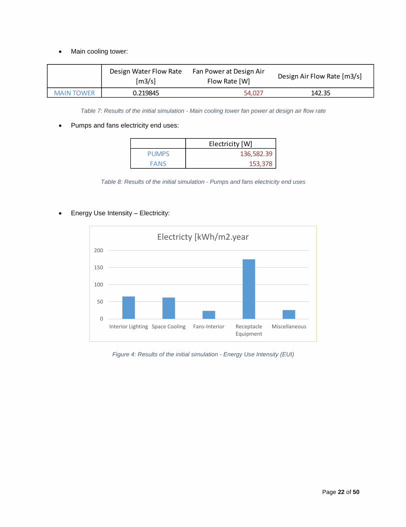
Energy Use Intensity – Electricity:

Figure 4: Results of the initial simulation - Energy Use Intensity (EUI)

Design Water Flow Rate

[m3/s]

Fan Power at Design Air

Flow Rate [W]Design Air Flow Rate [m3/s]

MAIN TOWER 0.219845 54,027 142.35

Electricity [W]

PUMPS 136,582.39

FANS 153,378

0

50

100

150

200

Interior Lighting Space Cooling Fans-Interior ReceptacleEquipment

Miscellaneous

Electricty [kWh/m2.year

Page 23 of 50

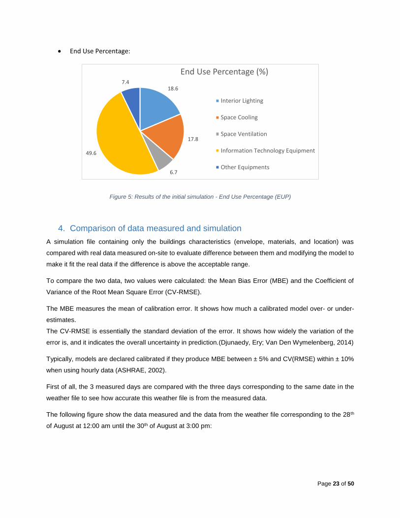
End Use Percentage:

Figure 5: Results of the initial simulation - End Use Percentage (EUP)

4. Comparison of data measured and simulation

A simulation file containing only the buildings characteristics (envelope, materials, and location) was

compared with real data measured on-site to evaluate difference between them and modifying the model to

make it fit the real data if the difference is above the acceptable range.

To compare the two data, two values were calculated: the Mean Bias Error (MBE) and the Coefficient of

Variance of the Root Mean Square Error (CV-RMSE).

The MBE measures the mean of calibration error. It shows how much a calibrated model over- or under-

estimates.

The CV-RMSE is essentially the standard deviation of the error. It shows how widely the variation of the

error is, and it indicates the overall uncertainty in prediction.(Djunaedy, Ery; Van Den Wymelenberg, 2014)

Typically, models are declared calibrated if they produce MBE between ± 5% and CV(RMSE) within ± 10%

when using hourly data (ASHRAE, 2002).

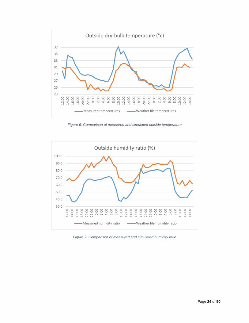
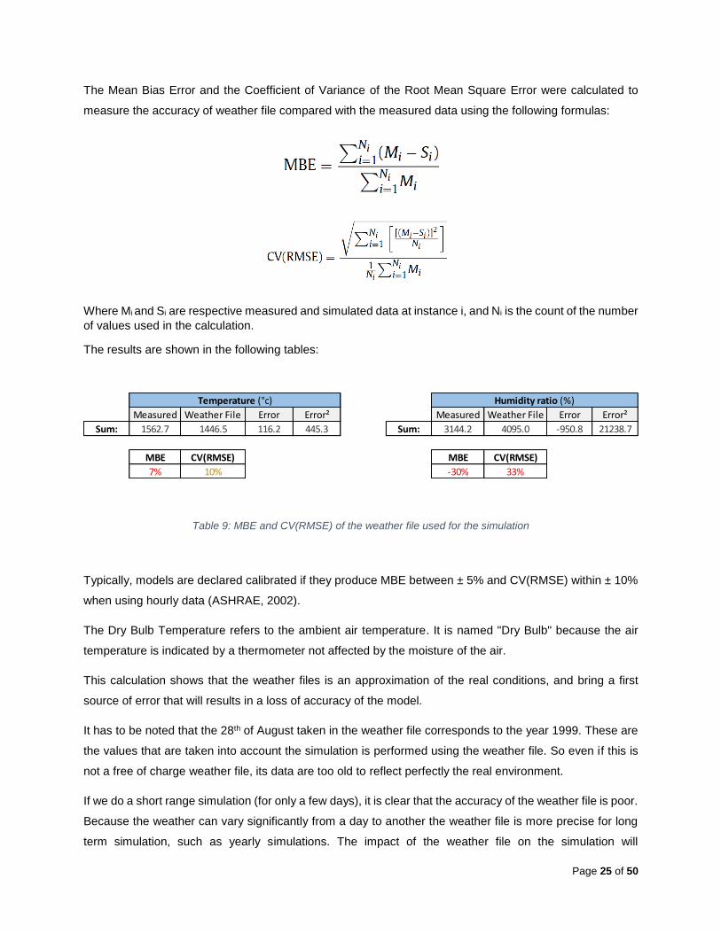
First of all, the 3 measured days are compared with the three days corresponding to the same date in the

weather file to see how accurate this weather file is from the measured data.

The following figure show the data measured and the data from the weather file corresponding to the 28 th

of August at 12:00 am until the 30th of August at 3:00 pm:

18.6

17.8

6.7

49.6

7.4

End Use Percentage (%)

Interior Lighting

Space Cooling

Space Ventilation

Information Technology Equipment

Other Equipments

Page 24 of 50

Figure 6: Comparison of measured and simulated outside temperature

Figure 7: Comparison of measured and simulated humidity ratio

23

25

27

29

31

33

35

37

12

:00

14

:00

16

:00

18

:00

20

:00

22

:00

0:0

0

2:0

0

4:0

0

6:0

0

8:0

0

10

:00

12

:00

14

:00

16

:00

18

:00

20

:00

22

:00

0:0

0

2:0

0

4:0

0

6:0

0

8:0

0

10

:00

12

:00

14

:00

Outside dry-bulb temperature (°c)

Measured temperatures Weather file temperatures

30.0

40.0

50.0

60.0

70.0

80.0

90.0

100.0

12

:00

14

:00

16

:00

18

:00

20

:00

22

:00

0:0

0

2:0

0

4:0

0

6:0

0

8:0

0

10

:00

12

:00

14

:00

16

:00

18

:00

20

:00

22

:00

0:0

0

2:0

0

4:0

0

6:0

0

8:0

0

10

:00

12

:00

14

:00

Outside humidity ratio (%)

Measured humidity ratio Weather file humidity ratio

Page 25 of 50

The Mean Bias Error and the Coefficient of Variance of the Root Mean Square Error were calculated to

measure the accuracy of weather file compared with the measured data using the following formulas:

Where Mi and Si are respective measured and simulated data at instance i, and Ni is the count of the number

of values used in the calculation.

The results are shown in the following tables:

Table 9: MBE and CV(RMSE) of the weather file used for the simulation

Typically, models are declared calibrated if they produce MBE between ± 5% and CV(RMSE) within ± 10%

when using hourly data (ASHRAE, 2002).

The Dry Bulb Temperature refers to the ambient air temperature. It is named "Dry Bulb" because the air

temperature is indicated by a thermometer not affected by the moisture of the air.

This calculation shows that the weather files is an approximation of the real conditions, and bring a first

source of error that will results in a loss of accuracy of the model.

It has to be noted that the 28th of August taken in the weather file corresponds to the year 1999. These are

the values that are taken into account the simulation is performed using the weather file. So even if this is

not a free of charge weather file, its data are too old to reflect perfectly the real environment.

If we do a short range simulation (for only a few days), it is clear that the accuracy of the weather file is poor.

Because the weather can vary significantly from a day to another the weather file is more precise for long

term simulation, such as yearly simulations. The impact of the weather file on the simulation will

Measured Weather File Error Error² Measured Weather File Error Error²

Sum: 1562.7 1446.5 116.2 445.3 Sum: 3144.2 4095.0 -950.8 21238.7

MBE CV(RMSE) MBE CV(RMSE)

7% 10% -30% 33%

Temperature (°c) Humidity ratio (%)

Page 26 of 50

unfortunately not be studied in the sensitivity analysis, since the software used (SimLab) does not include

this option.

Unfortunately, for the calibrated simulation, the measured data could not be implemented into the weather

because they don’t use the same format. So far the tool to convert one file to another format are not very

successful. The uncertainty due to the weather file has then to be considered.

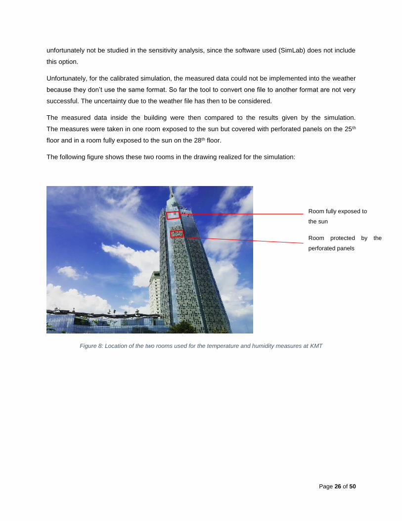
The measured data inside the building were then compared to the results given by the simulation.

The measures were taken in one room exposed to the sun but covered with perforated panels on the 25th

floor and in a room fully exposed to the sun on the 28th floor.

The following figure shows these two rooms in the drawing realized for the simulation:

Figure 8: Location of the two rooms used for the temperature and humidity measures at KMT

Room fully exposed to

the sun

Room protected by the

perforated panels

Page 27 of 50

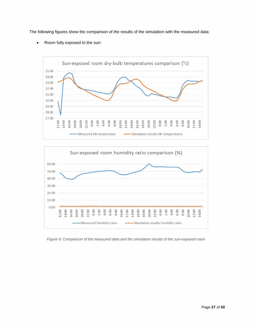
The following figures show the comparison of the results of the simulation with the measured data:

Room fully exposed to the sun:

Figure 9: Comparison of the measured data and the simulation results of the sun-exposed room

Page 28 of 50

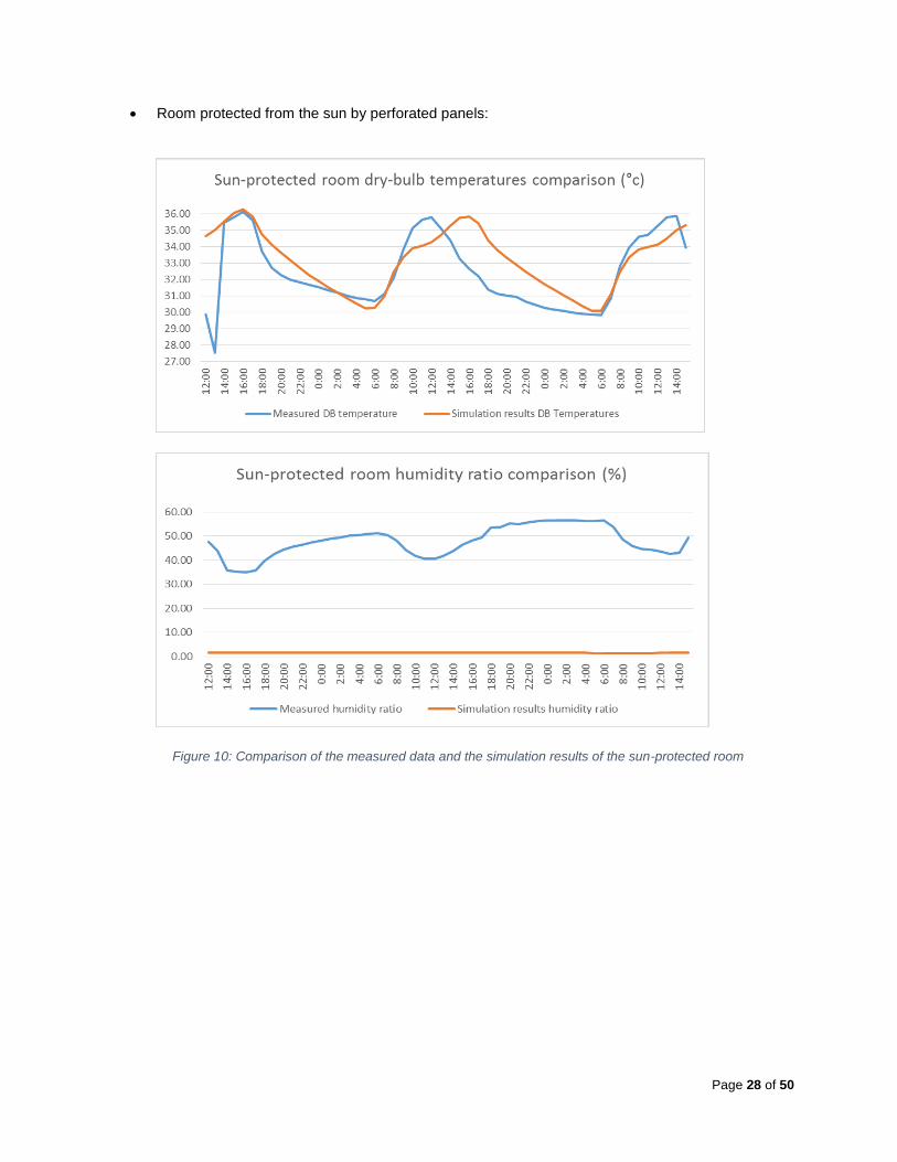
Room protected from the sun by perforated panels:

Figure 10: Comparison of the measured data and the simulation results of the sun-protected room

Page 29 of 50

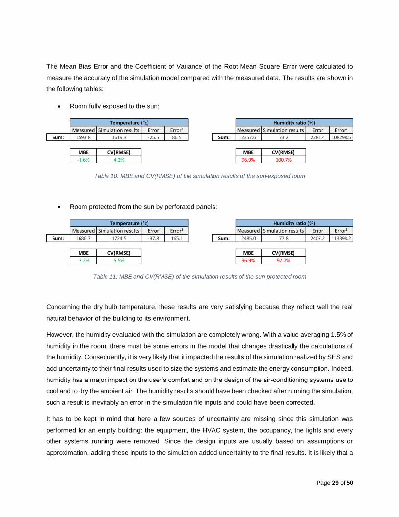
The Mean Bias Error and the Coefficient of Variance of the Root Mean Square Error were calculated to

measure the accuracy of the simulation model compared with the measured data. The results are shown in

the following tables:

Room fully exposed to the sun:

Table 10: MBE and CV(RMSE) of the simulation results of the sun-exposed room

Room protected from the sun by perforated panels:

Table 11: MBE and CV(RMSE) of the simulation results of the sun-protected room

Concerning the dry bulb temperature, these results are very satisfying because they reflect well the real

natural behavior of the building to its environment.

However, the humidity evaluated with the simulation are completely wrong. With a value averaging 1.5% of

humidity in the room, there must be some errors in the model that changes drastically the calculations of

the humidity. Consequently, it is very likely that it impacted the results of the simulation realized by SES and

add uncertainty to their final results used to size the systems and estimate the energy consumption. Indeed,

humidity has a major impact on the user’s comfort and on the design of the air-conditioning systems use to

cool and to dry the ambient air. The humidity results should have been checked after running the simulation,

such a result is inevitably an error in the simulation file inputs and could have been corrected.

It has to be kept in mind that here a few sources of uncertainty are missing since this simulation was

performed for an empty building: the equipment, the HVAC system, the occupancy, the lights and every

other systems running were removed. Since the design inputs are usually based on assumptions or

approximation, adding these inputs to the simulation added uncertainty to the final results. It is likely that a

Measured Simulation results Error Error² Measured Simulation results Error Error²

Sum: 1593.8 1619.3 -25.5 86.5 Sum: 2357.6 73.2 2284.4 108298.5


-1.6% 4.2% 96.9% 100.7%


Measured Simulation results Error Error² Measured Simulation results Error Error²

Sum: 1686.7 1724.5 -37.8 165.1 Sum: 2485.0 77.8 2407.2 113398.2


-2.2% 5.5% 96.9% 97.7%


Page 30 of 50

calculation of the MBE and CV(RMSE) comparing the building running normally and the complete simulation

file would not have given such good results.

If SES had realized a test running their simulation file with the empty building, they would have noticed that

there were errors concerning the humidity estimations, even if they could not compare these values with

data measured (the building was still in a project stage).

Page 31 of 50

IV. Methodology

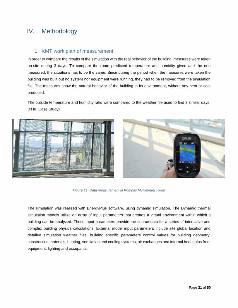
1. KMT work plan of measurement

In order to compare the results of the simulation with the real behavior of the building, measures were taken

on-site during 3 days. To compare the room predicted temperature and humidity given and the one

measured, the situations has to be the same. Since during the period when the measures were taken the

building was built but no system nor equipment were running, they had to be removed from the simulation

file. The measures show the natural behavior of the building in its environment, without any heat or cool

produced.

The outside temperature and humidity ratio were compared to the weather file used to find 3 similar days.

(cf III. Case Study)

Figure 11: Data measurement in Kompas Multimedia Tower

The simulation was realized with EnergyPlus software, using dynamic simulation. The Dynamic thermal

simulation models utilize an array of input parameters that creates a virtual environment within which a

building can be analyzed. These input parameters provide the source data for a series of interactive and

complex building physics calculations. External model input parameters include site global location and

detailed simulation weather files: building specific parameters control values for building geometry,

construction materials, heating, ventilation and cooling systems, air exchanges and internal heat gains from

equipment, lighting and occupants.

Page 32 of 50

2. Software used

How e+ works:

EnergyPlus is an energy analysis and thermal load simulation program. EnergyPlus processes text input

into text output using the EnergyPlus engine. For example, the user enters the basics of the building and

the software will output the energy bills, the annual energy consumption, zone temperatures, HVAC system

size and so on.

Since EnergyPlus uses text-in, text-out approach, it can be coupled with many Graphical User Interfaces

(GUIs) to make it easier to use. In order to facilitate the use of EnergyPlus to add the details on the Sketchup

drawing of the building, the Openstudio plug-in was used in this study providing a user-friendly interface.

Why EnergyPlus:

Energy simulation software tools for buildings have had developments over the years. Currently there are

several energy simulation software tools with different levels of complexity and response to different

variables. Among the most complete simulation software tools are the Energy Plus, the ESP-r (Energy

Simulation Software tool), the IDA ICE (Indoor Climate Energy), IES-VE (Integrated Environmental Solutions

- Virtual Environment) and TRNSYS. Being the most complete software tools, these are also the most

complex and therefore require greater expertise. (Sousa, 2012)

EnergyPlus is one of the most authoritative and has been extensively used and validated by the research

community. It has several user interface add-ons and is the result of 60 years of development by the US

department of energy.

This work aims at evaluating the factors that impact the most the results of this widely used energy

simulation software.

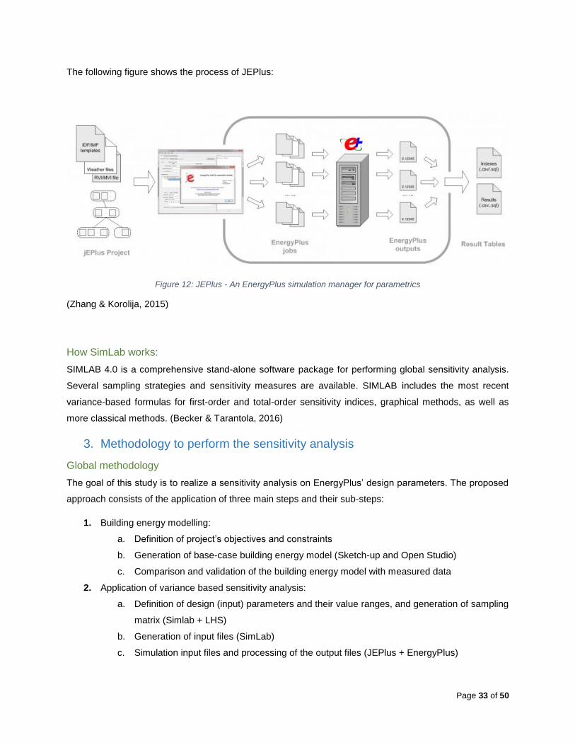
How JEPlus works:

Parametric analysis is often needed for exploring design options, especially when a global optimization

method is not available, or the optimization result is in doubt. Parametric analysis can also be applied to all

design variables simultaneously, which forms an exhaustive search that, on a fine mesh, enables the

discovery of the global optimum solution. To perform complex parametric analysis on multiple design

parameters, a tool is needed to create and manage simulation jobs, and to collect results afterwards. jEPlus

has been developed for this purpose. (Zhang & Korolija, 2015)

Page 33 of 50

The following figure shows the process of JEPlus:

Figure 12: JEPlus - An EnergyPlus simulation manager for parametrics

(Zhang & Korolija, 2015)

How SimLab works:

SIMLAB 4.0 is a comprehensive stand-alone software package for performing global sensitivity analysis.

Several sampling strategies and sensitivity measures are available. SIMLAB includes the most recent

variance-based formulas for first-order and total-order sensitivity indices, graphical methods, as well as

more classical methods. (Becker & Tarantola, 2016)

3. Methodology to perform the sensitivity analysis

Global methodology

The goal of this study is to realize a sensitivity analysis on EnergyPlus’ design parameters. The proposed

approach consists of the application of three main steps and their sub-steps:

1. Building energy modelling:

a. Definition of project’s objectives and constraints

b. Generation of base-case building energy model (Sketch-up and Open Studio)

c. Comparison and validation of the building energy model with measured data

2. Application of variance based sensitivity analysis:

a. Definition of design (input) parameters and their value ranges, and generation of sampling

matrix (Simlab + LHS)

b. Generation of input files (SimLab)

c. Simulation input files and processing of the output files (JEPlus + EnergyPlus)

Page 34 of 50

d. Collect and analyze of the simulation’s outputs (SimLab + Microsoft Excel)

3. Analysis of the results

a. Calculation of the sensitivity indices of input parameters (Simlab + Excel)

b. Overview of the PEAR, SRC and PCC methods results

c. Ranking the input parameters per importance on the output variable using the PEAR

method

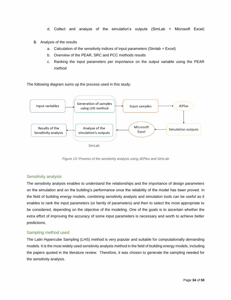
The following diagram sums up the process used in this study:

Figure 13: Process of the sensitivity analysis using JEPlus and SimLab

Sensitivity analysis

The sensitivity analysis enables to understand the relationships and the importance of design parameters

on the simulation and on the building’s performance once the reliability of the model has been proved. In

the field of building energy models, combining sensitivity analysis and simulation tools can be useful as it

enables to rank the input parameters (or family of parameters) and then to select the most appropriate to

be considered, depending on the objective of the modeling. One of the goals is to ascertain whether the

extra effort of improving the accuracy of some input parameters is necessary and worth to achieve better

predictions.

Sampling method used

The Latin Hypercube Sampling (LHS) method is very popular and suitable for computationally demanding

models. It is the most widely used sensitivity analysis method in the field of building energy models, including

the papers quoted in the literature review. Therefore, it was chosen to generate the sampling needed for

the sensitivity analysis.

Page 35 of 50

How the Latin Hypercube Sampling works

The LHS methods divides the cumulative curve into equal intervals on the cumulative probability scale, then

takes a random value from each interval of the input distribution (the number of intervals equals the number

of iterations). The samples generated are therefore not pure random, but random samples divided into

levels. The effect is that each sample (the data of each simulation) is constrained to match the input

distribution very closely. Therefore, even for modest numbers of iterations, this method makes all or nearly

all sample means fall within a small fraction of the standard error. When performing multiple simulations,

their means will be much closer together with Latin Hypercube than with Monte Carlo, another widely used

sampling method.

Statistical methods

The results depend on which statistical method is selected to measure the linear correlation between the

inputs and the outputs. To choose which method to perform in this study, the results of several papers

evaluating the accuracy and the complexity of the different methods were put together (cf II. Literature

review). The Pearson product moment correlation coefficients (PEAR), the Partial Correlation Coefficient

(PCC) and the Standardized Regression Coefficient (SRC) were calculated as they offer a great

compromise between accuracy and computational cost in building energy models. (Nguyen & Reiter, 2015)

Pearson product moment correlation coefficient (PEAR)

The Pearson product-moment correlation coefficient (Pearson’s correlation, for short) is a measure of the

strength and direction of association that exists between two variables measured on at least an interval

scale. A Pearson’s correlation attempts to draw a line of best fit through the data of two variables, and the

Pearson correlation coefficient, r, indicates how far away all these data points are from this line of best fit.

Partial Correlation Coefficient (PCC)

Partial correlation measures the degree of association between two random variables, with the effect of a

set of controlling random variables removed. If we are interested in finding whether or to what extent there

is a numerical relationship between two variables of interest, using their correlation coefficient will give

misleading results if there is another, confounding, variable that is numerically related to both variables of

interest. This misleading information can be avoided by controlling for the confounding variable, which is

done by computing the partial correlation coefficient.

Standardized Regression Coefficient (SRC)

Standardized coefficients are the estimates resulting from a regression analysis that have been

standardized so that the variances of dependent and independent variables are 1. Therefore, standardized

coefficients refer to how many standard deviations a dependent variable will change, per standard deviation

increase in the predictor variable. For one-dimensional regression, the absolute value of the standardized

coefficient equals the correlation coefficient. Standardization of the coefficient is usually done to answer the

Page 36 of 50

question of which of the independent variables have a greater effect on the dependent variable in a multiple

regression analysis, when the variables are measured in different units of measurement.

Choice of design parameters to study

Many design parameters set in the simulation are based on assumptions and approximations. The standard

values recommended by the ASHRAE Guidelines are often used in case of lack of data or if some situations

are complex to evaluate (e.g. people occupancy). Here, as an example, are described the data that had

been gathered by the company to help them perform the simulation:

HVAC system to be installed: Fan Coil Unit (FCU) , supplied by water cooled magnetic chiller

Most common light bulbs to be installed: LED will be used in most of the room

How many light bulbs per square meter in common rooms: Not sure of the exact value to be installed

Total number of people that will work in the tower: Not decided yet

Average number of people for common rooms: Not decided yet

Occupancy schedules: Hard to determinate

Temperature set points in common rooms and in IT rooms: Depends of the user but around 23°c

These information are very vague, but the consultancy company had to decide of a value for every

parameter anyway to perform the simulation. Hence the use of guidelines and approximated values.

The goal of this work is to evaluate how the design parameters will impact the results of the simulation, to

know if it would be worth to investigate more on some of them to improve their accuracy and therefore

reduce the uncertainty of the results.

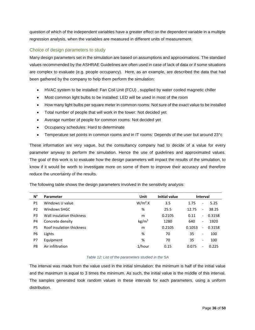
The following table shows the design parameters involved in the sensitivity analysis:

N° Parameter Unit Initial value Interval

P1 Windows U value W/m².K 3.5 1.75 - 5.25

P2 Windows SHGC % 25.5 12.75 - 38.25

P3 Wall insulation thickness m 0.2105 0.11 - 0.3158

P4 Concrete density kg/m3 1280 640 - 1920

P5 Roof insulation thickness m 0.2105 0.1053 - 0.3158

P6 Lights % 70 35 - 100

P7 Equipment % 70 35 - 100

P8 Air infiltration 1/hour 0.15 0.075 - 0.225

Table 12: List of the parameters studied in the SA

The interval was made from the value used in the initial simulation: the minimum is half of the initial value

and the maximum is equal to 3 times the minimum. As such, the initial value is the middle of this interval.

The samples generated took random values in these intervals for each parameters, using a uniform

distribution.

Page 37 of 50

The concrete is used in the structure of the building, in every exterior wall and in the roof. The

parameter ‘’concrete density’’ shows the impact of the density of the structure in the simulation.

The lights and equipment correspond to the percentage used during the week days out of the

capacity attributed to each zone.

The windows U value corresponds to the windows overall heat transfer coefficient.

The windows SHGC corresponds to the windows Solar Heat Gain Coefficient.

The air infiltration corresponds to the air changes per hour due to the natural ventilation. 0.15

changes per hour means that the air inside a room is completely renewed every 6 hours and 40

minutes.

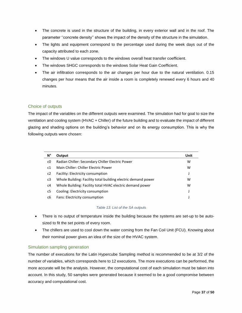
Choice of outputs

The impact of the variables on the different outputs were examined. The simulation had for goal to size the

ventilation and cooling system (HVAC + Chiller) of the future building and to evaluate the impact of different

glazing and shading options on the building’s behavior and on its energy consumption. This is why the

following outputs were chosen:

N° Output Unit

c0 Radian Chiller: Secondary Chiller Electric Power W

c1 Main Chiller: Chiller Electric Power W

c2 Facility: Electricity consumption J

c3 Whole Building: Facility total building electric demand power W

c4 Whole Building: Facility total HVAC electric demand power W

c5 Cooling: Electricity consumption J

c6 Fans: Electricity consumption J

Table 13: List of the SA outputs

There is no output of temperature inside the building because the systems are set-up to be auto-

sized to fit the set points of every room.

The chillers are used to cool down the water coming from the Fan Coil Unit (FCU). Knowing about

their nominal power gives an idea of the size of the HVAC system.

Simulation sampling generation

The number of executions for the Latin Hypercube Sampling method is recommended to be at 3/2 of the

number of variables, which corresponds here to 12 executions. The more executions can be performed, the

more accurate will be the analysis. However, the computational cost of each simulation must be taken into

account. In this study, 50 samples were generated because it seemed to be a good compromise between

accuracy and computational cost.

Page 38 of 50

The samples were generated using Simlab and the 50 simulations are then run by JEPlus using EnergyPlus

engine. Then the outputs are adapted through Excel to be processed with Simlab and PEAR, SRC and PRC

sensitivity indices were calculated.

The PEAR will be more detailed in this study to detail the sensitivity of the variables.

Page 39 of 50

V. Results

After generating the samples using SimLab, JEPlus has been used to manage the 50 simulations realized

with EnergyPlus. The outputs of the simulations were then analyzed with SimLab to perform the sensitivity

analysis.

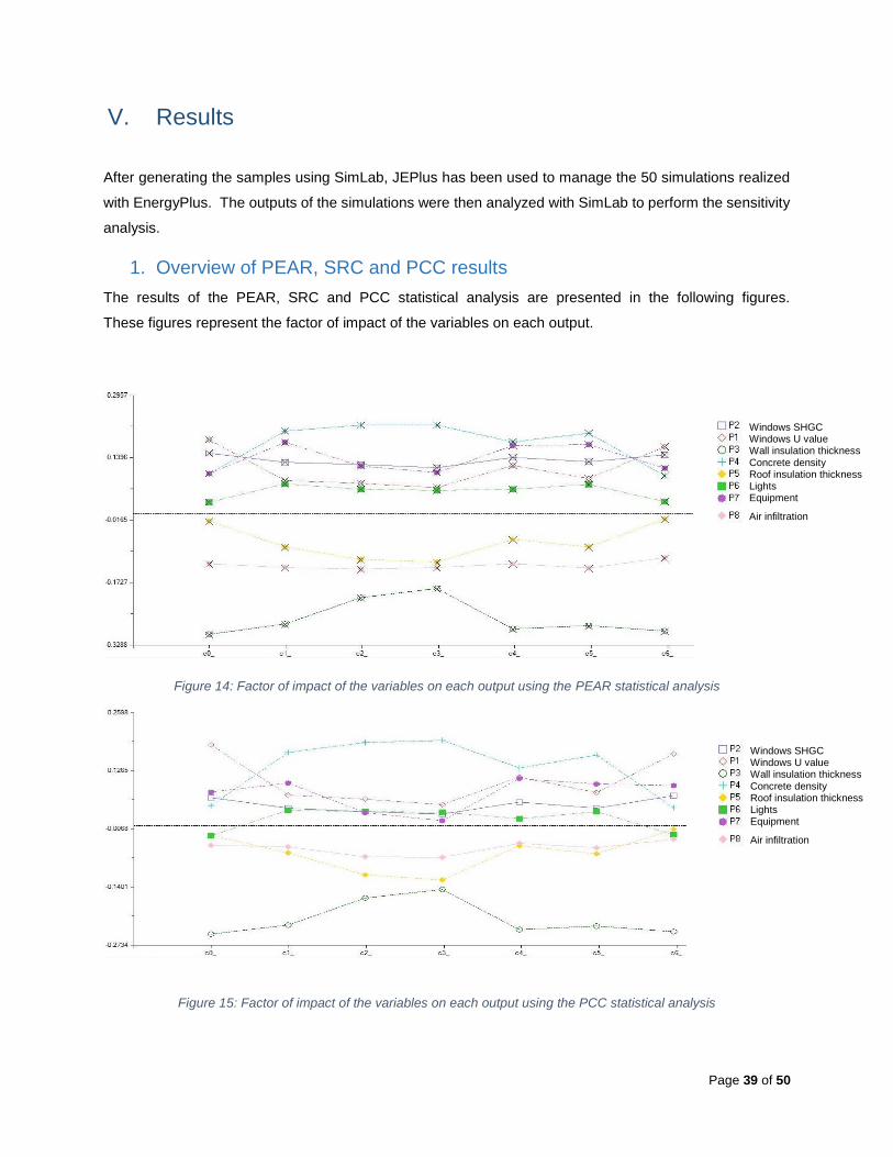
1. Overview of PEAR, SRC and PCC results

The results of the PEAR, SRC and PCC statistical analysis are presented in the following figures.

These figures represent the factor of impact of the variables on each output.

Figure 14: Factor of impact of the variables on each output using the PEAR statistical analysis

Figure 15: Factor of impact of the variables on each output using the PCC statistical analysis

Windows SHGC Windows U value Wall insulation thickness Concrete density Roof insulation thickness Lights Equipment

Air infiltration


Air infiltration

Page 40 of 50

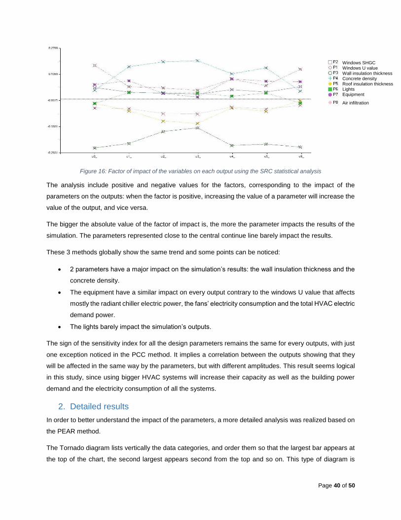
Figure 16: Factor of impact of the variables on each output using the SRC statistical analysis

The analysis include positive and negative values for the factors, corresponding to the impact of the

parameters on the outputs: when the factor is positive, increasing the value of a parameter will increase the

value of the output, and vice versa.

The bigger the absolute value of the factor of impact is, the more the parameter impacts the results of the

simulation. The parameters represented close to the central continue line barely impact the results.

These 3 methods globally show the same trend and some points can be noticed:

2 parameters have a major impact on the simulation’s results: the wall insulation thickness and the

concrete density.

The equipment have a similar impact on every output contrary to the windows U value that affects

mostly the radiant chiller electric power, the fans’ electricity consumption and the total HVAC electric

demand power.

The lights barely impact the simulation’s outputs.

The sign of the sensitivity index for all the design parameters remains the same for every outputs, with just

one exception noticed in the PCC method. It implies a correlation between the outputs showing that they

will be affected in the same way by the parameters, but with different amplitudes. This result seems logical

in this study, since using bigger HVAC systems will increase their capacity as well as the building power

demand and the electricity consumption of all the systems.

2. Detailed results

In order to better understand the impact of the parameters, a more detailed analysis was realized based on

the PEAR method.

The Tornado diagram lists vertically the data categories, and order them so that the largest bar appears at

the top of the chart, the second largest appears second from the top and so on. This type of diagram is


Air infiltration

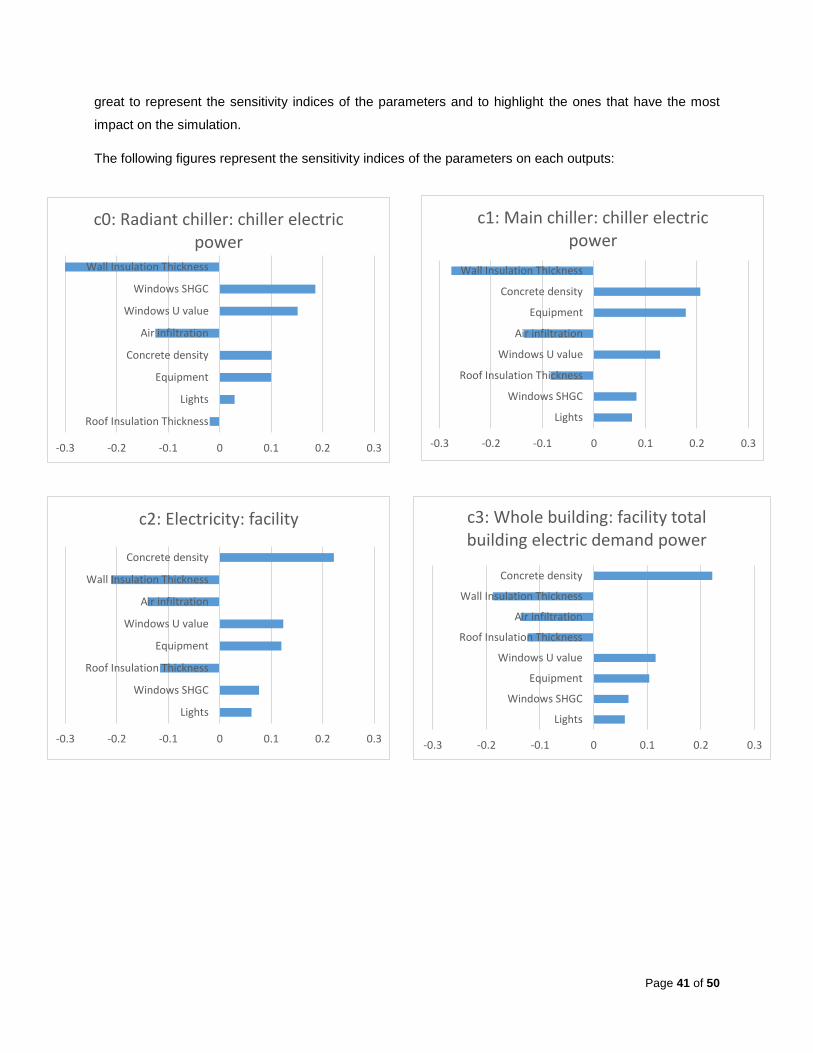
Page 41 of 50

great to represent the sensitivity indices of the parameters and to highlight the ones that have the most

impact on the simulation.

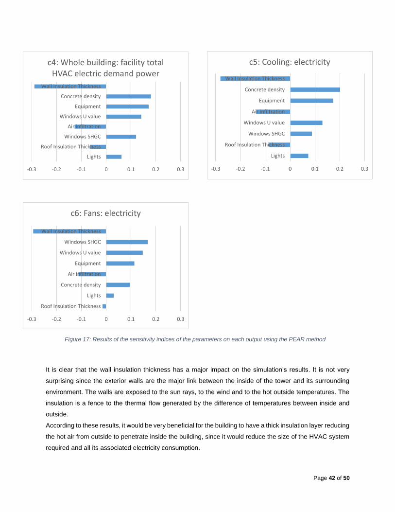
The following figures represent the sensitivity indices of the parameters on each outputs:

-0.3 -0.2 -0.1 0 0.1 0.2 0.3

Lights

Windows SHGC

Roof Insulation Thickness

Windows U value

Air infiltration

Equipment

Concrete density

Wall Insulation Thickness

c1: Main chiller: chiller electric power

-0.3 -0.2 -0.1 0 0.1 0.2 0.3


Lights

Equipment

Concrete density

Air infiltration

Windows U value

Windows SHGC


c0: Radiant chiller: chiller electric power

-0.3 -0.2 -0.1 0 0.1 0.2 0.3

Lights

Windows SHGC


Equipment

Windows U value

Air infiltration


Concrete density

c2: Electricity: facility

-0.3 -0.2 -0.1 0 0.1 0.2 0.3

Lights

Windows SHGC

Equipment

Windows U value


Air infiltration


Concrete density

c3: Whole building: facility total building electric demand power

Page 42 of 50

It is clear that the wall insulation thickness has a major impact on the simulation’s results. It is not very

surprising since the exterior walls are the major link between the inside of the tower and its surrounding

environment. The walls are exposed to the sun rays, to the wind and to the hot outside temperatures. The

insulation is a fence to the thermal flow generated by the difference of temperatures between inside and

outside.

According to these results, it would be very beneficial for the building to have a thick insulation layer reducing

the hot air from outside to penetrate inside the building, since it would reduce the size of the HVAC system

required and all its associated electricity consumption.

-0.3 -0.2 -0.1 0 0.1 0.2 0.3

Lights


Windows SHGC

Air infiltration

Windows U value

Equipment

Concrete density


c4: Whole building: facility total HVAC electric demand power

-0.3 -0.2 -0.1 0 0.1 0.2 0.3

Lights


Windows SHGC

Windows U value

Air infiltration

Equipment

Concrete density


c5: Cooling: electricity

-0.3 -0.2 -0.1 0 0.1 0.2 0.3


Lights

Concrete density

Air infiltration

Equipment

Windows U value

Windows SHGC


c6: Fans: electricity

Figure 17: Results of the sensitivity indices of the parameters on each output using the PEAR method

Page 43 of 50

On the contrary, increasing the density of the concrete used in of the wall’s and roof’s layer increases the

HVAC needs. This happens because it increases the thermal mass of the walls, therefore the quantity of

heat that can be stored by the facade. The heat is then released in the building even when the outside

temperature decreases below the building’s average temperature. The concrete density often appears also

of major influence on the simulation.

Concerning the windows characteristics, their overall heat transfer coefficient (U value) seems to have

slightly more impact on the simulation’s results than their Solar Heat Gain Coefficient (SHGC). Besides, it

is satisfying to see that the SHGC can have a significant impact on the simulation, meaning that the sun

rays are really taken into account into the EnergyPlus calculation model. So studying the impact of the

implementation of shading devices or solar films using dynamic simulations makes sense and has potential.

As supposed, the roof’s insulation thickness impact on the simulation is much lower than the wall’s insulation

thickness since the area covered is smaller.

The impact of air infiltration on the simulation seems contradictory with what could be expected: increasing

it reduces the HVAC needs. It can be explained by the natural ventilation effect when the outside air

penetrates the building. Knowing that in a day there are more hours when the outside temperature is lower

that the temperature inside the building, it helps the HVAC systems cooling down in these hours. Reducing

the air infiltration also increase the needs of mechanical ventilation required to guarantee a good air quality

inside the building bringing ‘’new air’’ from outside, and by consequence the electrical consumption.

The role of adding the equipment and the lighting to the simulation is to add their heating and electricity

loads in the calculations. As expected, the more they are used and the more the building needs to be cooled

down, and the bigger is the energy consumption. The energy consumption is affected in two points: the

equipment and lighting consume directly electricity to run, and they release heat that need to be

compensated by the cooling systems that also consume electricity to run.

The electricity consumption and the heat release associated to the lighting are in smaller proportion than

the equipment, explaining the modest impact of the lighting on the simulation.

The initial simulation was performed by the company using either standard values or assumptions for every

parameters. Even if standard values can be a good approximation, it is hard to know to what extend they

approach the reality of each building. Using accurate inputs in the simulations is very difficult in most of the

projects for several reasons:

Technical details are missing

The manager does not know exactly how will be built / how has been built the building

It is difficult to know at what power will run the systems

Some technical aspects have not been decided yet

Some phenomena such as people behavior are complicated to predict

Page 44 of 50

Even when the power of a system is given, the ratio of the energy converted to heat is not given or

approximate

The physical processes used by the software are simplified so they do not reflect exactly the real

phenomena (e.g. HVAC system does not consider losses of heat and cold in the pipes)

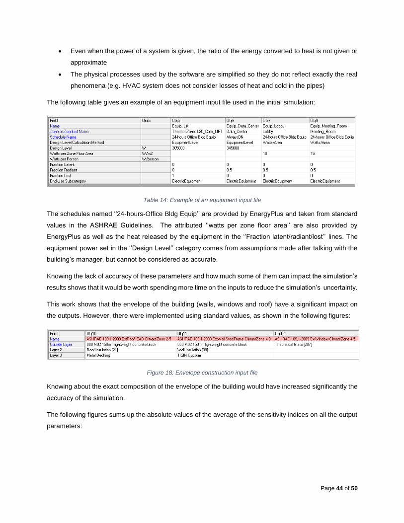
The following table gives an example of an equipment input file used in the initial simulation:

Table 14: Example of an equipment input file

The schedules named ‘’24-hours-Office Bldg Equip’’ are provided by EnergyPlus and taken from standard

values in the ASHRAE Guidelines. The attributed ‘’watts per zone floor area’’ are also provided by

EnergyPlus as well as the heat released by the equipment in the ‘’Fraction latent/radiant/lost’’ lines. The

equipment power set in the ‘’Design Level’’ category comes from assumptions made after talking with the

building’s manager, but cannot be considered as accurate.

Knowing the lack of accuracy of these parameters and how much some of them can impact the simulation’s

results shows that it would be worth spending more time on the inputs to reduce the simulation’s uncertainty.

This work shows that the envelope of the building (walls, windows and roof) have a significant impact on

the outputs. However, there were implemented using standard values, as shown in the following figures:

Figure 18: Envelope construction input file

Knowing about the exact composition of the envelope of the building would have increased significantly the

accuracy of the simulation.

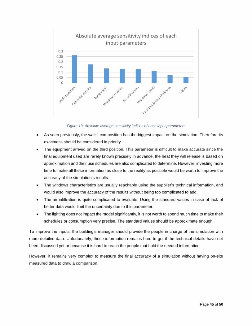
The following figures sums up the absolute values of the average of the sensitivity indices on all the output

parameters:

Page 45 of 50

Figure 19: Absolute average sensitivity indices of each input parameters

As seen previously, the walls’ composition has the biggest impact on the simulation. Therefore its

exactness should be considered in priority.

The equipment arrived on the third position. This parameter is difficult to make accurate since the

final equipment used are rarely known precisely in advance, the heat they will release is based on

approximation and their use schedules are also complicated to determine. However, investing more

time to make all these information as close to the reality as possible would be worth to improve the

accuracy of the simulation’s results.

The windows characteristics are usually reachable using the supplier’s technical information, and

would also improve the accuracy of the results without being too complicated to add.

The air infiltration is quite complicated to evaluate. Using the standard values in case of lack of

better data would limit the uncertainty due to this parameter.

The lighting does not impact the model significantly, it is not worth to spend much time to make their

schedules or consumption very precise. The standard values should be approximate enough.

To improve the inputs, the building’s manager should provide the people in charge of the simulation with

more detailed data. Unfortunately, these information remains hard to get if the technical details have not

been discussed yet or because it is hard to reach the people that hold the needed information.

However, it remains very complex to measure the final accuracy of a simulation without having on-site

measured data to draw a comparison.

0

0.05

0.1

0.15

0.2

0.25

0.3

Absolute average sensitivity indices of each input parameters

Page 46 of 50

VI. Discussion

The scope of this work was to address the performance gap that exists between predicted and operational

building energy performance, and to provide tracks to reduce this gap.

This work was very limited due to the computation cost of the simulation and the non-professional equipment

used. It would have been more relevant to realize a sensitivity analysis comparing the impact of more input

parameters.

It was showed that most of the parameters based on standard values and approximations have a significant

impact on the results. Some of them should be easy to make more accurate by searching more precise data

and technical information. Therefore, there is potential to improve the accuracy of the simulations, reducing

the uncertainty due to the input parameters without excessive time investment. However, some data will

remain very complicated to improve because there are based on assumptions such as the schedules, or

depend of complex phenomena such the air infiltration.

The paper Application of sensitivity analysis in building energy simulations: Combining first- and second-

order elementary effects methods also highlights the importance of the insulation thickness in the simulation.

However, two parameters that were not studied during this work appears in their study as of significant

impact on the results of the simulation: the ventilation rate and the set point temperature. Since our case

study considered an empty building, these parameters could not be considered.

(Sanchez et al., 2014)

Anh-Tuan Nguyen and Sigrid Reiter showed in their study that the external wall type, the thickness of internal

walls (thermal mass) and the size of window overhangs play a major role in the simulation’s outputs. This

is in line with the results with our sensitivity analysis showing that the building’s envelope is significant.


Simulations results should be treated cautiously since it is for now impossible to measure the accuracy of

the results. The results can be used to have an idea of the approximate size required of some systems such

as the HVAC or to compare the impact on the building’s behavior of different solutions such as the

implementation of different shading devices. So far, there is no outstanding solutions to measure the

precision of the simulations based on the precision of the parameters, without comparing them to on-site

measured data. This solution is not applicable if the building is not yet built or being used at the time of the

simulation. The best way is to compare the values obtained to measured data on comparable buildings.

It would have been interesting to perform sensitivity analysis on various types of buildings, to establish a

reference of the parameters that influence the most the simulations in different contexts.

These influential parameters will probably differs within different countries, unfortunately JEplus does not

propose to use the weather file as an input and to add in in the sensitivity analysis.

Page 47 of 50

Calibrating the model before performing the simulation is another great way to improve the simulations

accuracy. The simplest way is to calibrate the weather file using data measured on-site to the weather file

used for the simulation. A more complete calibration would be to compare the results of the simulations with

data measured inside the building in the same conditions. Indeed, calibrated whole building simulation is

recognized as the most effective way of predicting the impact of large scale interactive retrofit interventions.

Models can be calibrated against real monitoring data from existing buildings to produce a baseline which

is then used to more accurately estimate the impact of energy efficiency and carbon reduction measures.

Unfortunately this method requires the building to be already built and maybe some equipment to be running,

so it could only be used for building’s retrofit projects.

Several studies address the performance gap and improve the accuracy and quality of building simulation

using a combination of detailed calibrated dynamic thermal simulation models, detailed site measurement

and testing, in-use monitoring and Hygrothermal.

Page 48 of 50

VII. Conclusions

The main target of this thesis was to ascertain whether improving the input parameters accuracy worth to

achieve better predictions. The importance level of the parameters was measured through a sensitivity

analysis made on a simulation of a tower building in Jakarta, Indonesia.

The analysis of the results showed that the impact on the simulation’s results depends on the type of inputs.

It was found that some parameters that have a major influence on the outputs can be easily made more

precise such as the wall’s characteristics. Moreover some parameters that are complex to estimate can also

impact the accuracy of the results, such as the air infiltration rate through the building’s envelope.

The uncertainty in these inputs parameters can be due to a lack of technical information about the building

and its systems and due to assumptions that are difficult to make in the context of the project.

To partially solve this issue, standard values provided by the American Society of Heating, Refrigerating

and Air-Conditioning Engineers (ASHRAE) Guidelines are very often used. However, even if standard

values can be a good approximation, it is hard to know to what extend they approach the reality of each

buildings.

This work shows that the envelope of the building (walls, widows and roof) have a significant impact on the

outputs. However, there were implemented using standard values. Knowing about the exact composition of

the envelope of the building would have increased significantly the accuracy of the simulation, and these

information should be accessible.

Calibrating the model before performing the simulation is another great way to improve the simulations

accuracy. The simplest way is to calibrate the weather file using data measured on-site to the weather file

used for the simulation. A more complete calibration would be to compare the results of the simulations with

data measured inside the building in the same conditions. Unfortunately this method requires the building

to be already built and maybe some equipment to be running, so it could only be used for building’s retrofit

projects.

Page 49 of 50

VIII. References

ASHRAE. (2002). Measurement of energy and demand savings. ASHARE Guidelines 14-2002, 8400, 1–165.

Beattie, k. H., & Ward, I. C. (2017). THE ADVANTAGES OF BUILDING SIMULATION FOR BUILDING DESIGN ENGINEERS. Dublin Institute of Technology, The University of Sheffield, 1–6.

Becker, william E., & Tarantola, S. (2016). Simlab Software for Uncertainty and Sensitivity Analysis. Ec.europa, 6–7. https://doi.org/10.1007/978-3-319-12385-1

CeBe, C. for the B. E., & LSI, L. S. I. (2015). Building performance modelling.

Djunaedy, Ery; Van Den Wymelenberg, K. (2014). Targeted Calibration of Energy Models for Existing Building. ASHRAE Annual Conference, C038(SE-14), 1–8.

Global Alliance for Buildings and Construction. (2016). Towards Zero-Emission Efficient and Resilient Buildings: Global Status Report 2016, 1–32.

Huchuk, B., O’Brien, W., & Cruickshank, C. A. (2013). Preliminary results of model predictive control of shading systems. Simulation Series, 45(8), 211–214. Retrieved from http://www.scopus.com/inward/record.url?eid=2-s2.0-84876853821&partnerID=tZOtx3y1

Macdonald, I. A., Clarke, J. A., & Strachan, P. A. (1999). Assessing uncertainty in building simulation. Energy Systems Research Unit, University of Strathclyde, Glasgow.

Nguyen, A.-T., & Reiter, S. (2015). A performance comparison of sensitivity analysis methods for building energy models. Building Simulation, 8(6), 651–664. https://doi.org/10.1007/s12273-015-0245-4

Royapoor, M., & Roskilly, T. (2015). Building model calibration using energy and environmental data. Energy and Buildings, 94, 109–120. https://doi.org/10.1016/j.enbuild.2015.02.050

Sanchez, D. G., Lacarrière, B., Musy, M., & Bourges, B. (2014). Application of sensitivity analysis in building energy simulations : Combining first- and second-order elementary effects methods. Energy & Buildings, 68, 741–750. https://doi.org/10.1016/j.enbuild.2012.08.048

Solmaz, A. S., Halicioglu, F. H., & Gunan, S. (2014). A simulation based optimization approach for determining the optimum energy saving solutions for buildings. Department of Architecture , Faculty of Architecture , Dokuz Eylul University , Izmir , Turkey Department of Construction Science , College of Architecture, The University of Texas.

Song, J., Wei, L., Sun, Y., & Tian, W. (2014). Implementation of Meta-modelling for Sensitivity Analysis in Building Energy Analysis. eSim 2014, 12. Retrieved from http://www.ibpsa.org/proceedings/eSimPapers/2014/3B.5.pdf

Sousa, J. (2012). Energy Simulation Software for Buildings: Review and Comparison. Information Technology for Energy Applications 2012, 6–7. Retrieved from http://citeseerx.ist.psu.edu/viewdoc/download?doi=10.1.1.416.7812&rep=rep1&type=pdf

Synergy Efficiency Solutions. (2015). Building Energy Simulation for Menara Kompas - Technical Report No. 14001-03.

Synergy Efficiency Solutions. (2017). Synergy Efficiency Solutions. Retrieved June 10, 2017, from http://www.synergyefficiency.solutions/

US Department of Energy, N. laboratory. (2016). Bring Us Your Genes. Energy Systems Integration Facility. Retrieved from http://www.nrel.gov/docs/fy16osti/66883.pdf

Zhang, D. Y., & Korolija, D. I. (2015). JEPlus – An EnergyPlus simulation manager for parametrics. Retrieved October 29, 2017, from http://www.jeplus.org/wiki/doku.php?id=docs:manual_1_7_intro

Page 50 of 50

Documents

Building Dynamic simulation uncertainty evaluation based