Embed Size (px)
Citation preview
Building economic decision-making capabilities of Chinese wool textile millsedited by Colin Brown, Scott Waldron, John Longworth and Zhao Yutian
ACIAR Technical Reports No. 60(printed version published in 2004)
Building economic decision-making capabilities of Chinese wool textile mills
Colin Brown, Scott Waldron, John Longworth and Zhao Yutian
Australian Centre for International Agricultural ResearchCanberra, 2005
Building economic decision-making capabilities of Chinese wool textile millsedited by Colin Brown, Scott Waldron, John Longworth and Zhao Yutian
ACIAR Technical Reports No. 60(printed version published in 2004)
The Australian Centre for International Agricultural Research (ACIAR) was established in June 1982 by an Act of the Australian Parliament. Its mandate is to help identify agricultural problems in developing countries and to commission collaborative research between Australian and developing country researchers in fi elds where Australia has a special research competence.
Where trade names are used this constitutes neither endorsement of nor discrimination against any product by the Centre.
ACIAR TECHNICAL REPORT SERIES
This series of publications contains technical information resulting from ACIAR-supported programs, projects and workshops (for which proceedings are not published), reports on Centre-supported fact-fi nding studies, or reports on other topics resulting from ACIAR activities. Publications in the series are distributed internationally to selected individuals and scientifi c institutions and are also available from ACIAR’s website www.aciar.gov.au.
© Australian Centre for International Agricultural Research, GPO Box 1571,Canberra, ACT 2601
Brown C., Waldron S., Longworth J. and Zhao Y. 2004.Building economic decision-making capabilities of Chinese wool textile mills.ACIAR Technical Reports No. 60, 108p.
ISBN 1 86320 495 4 (print) 1 86320 496 2 (online)
Cover design: Design One Solutions, Hall, AustraliaTechnical editing and typesetting: Sun Photoset Pty Ltd, Brisbane, AustraliaPrinting: Elect Printing, Canberra, Australia
Cover photos by members of the ACIAR project team show, clockwise from top-right: spindles at the Qifa Textile Group mill in Li County of Hebei Province; sheep grazing at the Duosaite State Farm in Siziwang Banner in Inner Mongolia Autonomous Region; hand shearing on Regiment 129 Production and Construction Corps Farm near Kuitun in Xinjiang Uygur Autonomous Region; and CAEGWOOL training workshop with wool textile mill managers held in Wuxi City in June 2004.
iiiBuilding economic decision-making capabilities of Chinese wool textile mills
edited by Colin Brown, Scott Waldron, John Longworth and Zhao YutianACIAR Technical Reports No. 60
(printed version published in 2004)
ForewordCHINA has the largest wool textile industry in the world and is Australia’s largest market for wool, accounting for about 40 per cent of Australia’s wool exports. Wool and wool textiles are the major trading items between China and Australia. These statistics empha-sise the economic importance of the continued viability of the Chinese textile industry to both China and Australia. As well, the connection between the Chinese wool industry and sustainable development of China’s pastoral region has seen a long involvement by ACIAR in China’s wool and wool textile industries.
Recent economic reforms and market developments have posed major challenges to the viability of most Chinese wool textile mills. The mills are under pressure to become more competitive, to introduce better enterprise management and to improve their environ-mental standards. Yet, in many cases decision tools or skills needed to improve manage-ment practices are lacking.
Wool textile enterprises are actively seeking ways to improve management practices and to adopt a more analytic approach to decision making. The models and analyses presented in this report are designed to assist wool textile mills as they implement new operational procedures, management practices and decision-making processes.
The overarching goal of the ACIAR project was to improve the long-term viability of Chinese wool textile mills by facilitating adaptation to the changing market and policy environment and improving the effi ciency of their operations. The core of the project was the adoption of a “whole-of-mill” approach to analysing key management deci-sions. These analyses were supported by three sub-projects which examined: the supply chain for imported raw materials; the sourcing of domestically produced wool; and the changing market for mill outputs.
This report presents analyses and fi ndings from the core “whole-of-mill” investiga-tion. In particular, it provides complete documentation for CAEGWOOL which is a signifi cant output from this ACIAR project. CAEGWOOL is an EXCEL-based model designed to make better use of data already collected by most mills to evaluate a range of key economic decisions faced by wool mill managers in China. For example, the model helps managers decide: which fi bre input combinations will minimise the cost of producing a particular fabric; what impact a specifi c piece of new processing or effl uent treatment technolgy will have on the overall profi tability of the mill; and what price to charge for a particular custom-processing order. An attached CD contains a working version of this model. ACIAR is very pleased to publish this report, which is also freely downloadable from our website at www.aciar.gov.au
Peter CoreDirectorAustralian Centre for International Agricultural Research
April 2005
ivBuilding economic decision-making capabilities of Chinese wool textile mills
edited by Colin Brown, Scott Waldron, John Longworth and Zhao YutianACIAR Technical Reports No. 60
(printed version published in 2004)
ContentsForeword . . . . . . . . . . . . . . . . . . . . . . . . . . . . . . . . . . . . . . . . . . . . . . . . . . . . . . . . . . . . . . . . . . . . . . . . . . . . . . iii
Figures . . . . . . . . . . . . . . . . . . . . . . . . . . . . . . . . . . . . . . . . . . . . . . . . . . . . . . . . . . . . . . . . . . . . . . . . . . . . . . . .vii
Tables . . . . . . . . . . . . . . . . . . . . . . . . . . . . . . . . . . . . . . . . . . . . . . . . . . . . . . . . . . . . . . . . . . . . . . . . . . . . . . . . viii
Preface . . . . . . . . . . . . . . . . . . . . . . . . . . . . . . . . . . . . . . . . . . . . . . . . . . . . . . . . . . . . . . . . . . . . . . . . . . . . . . . . ix
1. Introduction . . . . . . . . . . . . . . . . . . . . . . . . . . . . . . . . . . . . . . . . . . . . . . . . . . . . . . . . . . . . . . . . . . . . . . . . 1
1.1 Improving decision-making in Chinese wool textile mills . . . . . . . . . . . . . . . . . . . . . . . . . . . . . . 1
1.2 ACIAR involvement and Project ASEM/1998/060 . . . . . . . . . . . . . . . . . . . . . . . . . . . . . . . . . . . . 1
1.3 Synopsis . . . . . . . . . . . . . . . . . . . . . . . . . . . . . . . . . . . . . . . . . . . . . . . . . . . . . . . . . . . . . . . . . . . . . . 3
2. Allocating costs accurately . . . . . . . . . . . . . . . . . . . . . . . . . . . . . . . . . . . . . . . . . . . . . . . . . . . . . . . . . . . . 4
2.1 Broad approaches to estimating cost coeffi cients . . . . . . . . . . . . . . . . . . . . . . . . . . . . . . . . . . . . . 5
2.2 Statistical approach to estimating cost coeffi cients . . . . . . . . . . . . . . . . . . . . . . . . . . . . . . . . . . . . 5
2.2.1 Method of analysis . . . . . . . . . . . . . . . . . . . . . . . . . . . . . . . . . . . . . . . . . . . . . . . . . . . . . . . . 5
2.2.2 Data for analysis . . . . . . . . . . . . . . . . . . . . . . . . . . . . . . . . . . . . . . . . . . . . . . . . . . . . . . . . .5
2.2.3 Sources of data . . . . . . . . . . . . . . . . . . . . . . . . . . . . . . . . . . . . . . . . . . . . . . . . . . . . . . . . . . .6
2.2.4 Cost categories . . . . . . . . . . . . . . . . . . . . . . . . . . . . . . . . . . . . . . . . . . . . . . . . . . . . . . . . . . .7
2.2.5 Product types . . . . . . . . . . . . . . . . . . . . . . . . . . . . . . . . . . . . . . . . . . . . . . . . . . . . . . . . . . . .7
2.2.6 An alternative statistical approach . . . . . . . . . . . . . . . . . . . . . . . . . . . . . . . . . . . . . . . . . . .7
2.3 Analysis of cost coeffi cients for weaving . . . . . . . . . . . . . . . . . . . . . . . . . . . . . . . . . . . . . . . . . . . . 9
2.3.1 Product type approach . . . . . . . . . . . . . . . . . . . . . . . . . . . . . . . . . . . . . . . . . . . . . . . . . . . . .9
2.3.2 Alternative statistical approach . . . . . . . . . . . . . . . . . . . . . . . . . . . . . . . . . . . . . . . . . . . . . .9
2.4 Analysis of cost coeffi cients for spinning . . . . . . . . . . . . . . . . . . . . . . . . . . . . . . . . . . . . . . . . . . 10
2.4.1 Product type approach . . . . . . . . . . . . . . . . . . . . . . . . . . . . . . . . . . . . . . . . . . . . . . . . . . . .10
2.4.2 Alternative approach . . . . . . . . . . . . . . . . . . . . . . . . . . . . . . . . . . . . . . . . . . . . . . . . . . . . .11
2.5 Extensions . . . . . . . . . . . . . . . . . . . . . . . . . . . . . . . . . . . . . . . . . . . . . . . . . . . . . . . . . . . . . . . . . . . 11
3. Estimating yield coeffi cients . . . . . . . . . . . . . . . . . . . . . . . . . . . . . . . . . . . . . . . . . . . . . . . . . . . . . . . . . . 12
3.1 Approaches to estimating yield coeffi cients . . . . . . . . . . . . . . . . . . . . . . . . . . . . . . . . . . . . . . . . . 12
3.2 Data for analysis . . . . . . . . . . . . . . . . . . . . . . . . . . . . . . . . . . . . . . . . . . . . . . . . . . . . . . . . . . . . . .13
3.3 Processing yields . . . . . . . . . . . . . . . . . . . . . . . . . . . . . . . . . . . . . . . . . . . . . . . . . . . . . . . . . . . . . . 13
3.4 Finishing yields . . . . . . . . . . . . . . . . . . . . . . . . . . . . . . . . . . . . . . . . . . . . . . . . . . . . . . . . . . . . . . . 13
3.5 Weaving yields . . . . . . . . . . . . . . . . . . . . . . . . . . . . . . . . . . . . . . . . . . . . . . . . . . . . . . . . . . . . . . . . 16
3.6 Spinning yields . . . . . . . . . . . . . . . . . . . . . . . . . . . . . . . . . . . . . . . . . . . . . . . . . . . . . . . . . . . . . . . 16
3.7 Recombing/dyeing yields . . . . . . . . . . . . . . . . . . . . . . . . . . . . . . . . . . . . . . . . . . . . . . . . . . . . . . . 17
3.8 Discussion and implications . . . . . . . . . . . . . . . . . . . . . . . . . . . . . . . . . . . . . . . . . . . . . . . . . . . . . 18
iv
vBuilding economic decision-making capabilities of Chinese wool textile mills
edited by Colin Brown, Scott Waldron, John Longworth and Zhao YutianACIAR Technical Reports No. 60
(printed version published in 2004)
4. Analysing prices . . . . . . . . . . . . . . . . . . . . . . . . . . . . . . . . . . . . . . . . . . . . . . . . . . . . . . . . . . . . . . . . . . . 20
4.1 Analysis of the value of wool attributes . . . . . . . . . . . . . . . . . . . . . . . . . . . . . . . . . . . . . . . . . . . . 20
4.1.1 Analysis of Australian greasy wool auction prices . . . . . . . . . . . . . . . . . . . . . . . . . . . . . .22
4.1.2 Analysis of Nanjing Wool Market prices . . . . . . . . . . . . . . . . . . . . . . . . . . . . . . . . . . . . . .22
4.1.3 Analysis of Chinese wool auction prices . . . . . . . . . . . . . . . . . . . . . . . . . . . . . . . . . . . . . .26
4.1.4 Summary of implicit price analysis . . . . . . . . . . . . . . . . . . . . . . . . . . . . . . . . . . . . . . . . . .27
4.2 Market integration . . . . . . . . . . . . . . . . . . . . . . . . . . . . . . . . . . . . . . . . . . . . . . . . . . . . . . . . . . . . 27
4.2.1 Monthly price analysis . . . . . . . . . . . . . . . . . . . . . . . . . . . . . . . . . . . . . . . . . . . . . . . . . . . .27
4.2.2 Weekly analysis . . . . . . . . . . . . . . . . . . . . . . . . . . . . . . . . . . . . . . . . . . . . . . . . . . . . . . . . .27
4.2.3 Summary and implications of the integration analysis . . . . . . . . . . . . . . . . . . . . . . . . . . . 30
4.3 Price variation and relativities . . . . . . . . . . . . . . . . . . . . . . . . . . . . . . . . . . . . . . . . . . . . . . . . . . . 30
5. CAEGWOOL . . . . . . . . . . . . . . . . . . . . . . . . . . . . . . . . . . . . . . . . . . . . . . . . . . . . . . . . . . . . . . . . . . . . . 32
5.1 Introduction . . . . . . . . . . . . . . . . . . . . . . . . . . . . . . . . . . . . . . . . . . . . . . . . . . . . . . . . . . . . . . . . . . 32
5.1.1 Model philosophy . . . . . . . . . . . . . . . . . . . . . . . . . . . . . . . . . . . . . . . . . . . . . . . . . . . . . . . .32
5.1.2 Computer philosophy . . . . . . . . . . . . . . . . . . . . . . . . . . . . . . . . . . . . . . . . . . . . . . . . . . . . .33
5.2 The model . . . . . . . . . . . . . . . . . . . . . . . . . . . . . . . . . . . . . . . . . . . . . . . . . . . . . . . . . . . . . . . . . . . 33
5.2.1 Uses of the model . . . . . . . . . . . . . . . . . . . . . . . . . . . . . . . . . . . . . . . . . . . . . . . . . . . . . . . .33
5.2.2 Broad structure and assumptions of the model . . . . . . . . . . . . . . . . . . . . . . . . . . . . . . . . .33
5.2.3 Structure of the model . . . . . . . . . . . . . . . . . . . . . . . . . . . . . . . . . . . . . . . . . . . . . . . . . . . .34
5.2.4 Key model parameters . . . . . . . . . . . . . . . . . . . . . . . . . . . . . . . . . . . . . . . . . . . . . . . . . . . .34
5.3 CAEGWOOL Home page — navigating the CAEGWOOL spreadsheet . . . . . . . . . . . . . . . . . . 39
5.4 Input sheets . . . . . . . . . . . . . . . . . . . . . . . . . . . . . . . . . . . . . . . . . . . . . . . . . . . . . . . . . . . . . . . . . . 39
5.4.1 Front page sheet . . . . . . . . . . . . . . . . . . . . . . . . . . . . . . . . . . . . . . . . . . . . . . . . . . . . . . . . .39
5.4.2 Product design sheet . . . . . . . . . . . . . . . . . . . . . . . . . . . . . . . . . . . . . . . . . . . . . . . . . . . . .40
5.4.3 Cost input sheet . . . . . . . . . . . . . . . . . . . . . . . . . . . . . . . . . . . . . . . . . . . . . . . . . . . . . . . . .41
5.4.4 Price input sheet . . . . . . . . . . . . . . . . . . . . . . . . . . . . . . . . . . . . . . . . . . . . . . . . . . . . . . . .42
5.4.5 Product cost coeffi cients sheet . . . . . . . . . . . . . . . . . . . . . . . . . . . . . . . . . . . . . . . . . . . . . .42
5.4.6 Yield coeffi cients sheet . . . . . . . . . . . . . . . . . . . . . . . . . . . . . . . . . . . . . . . . . . . . . . . . . . . .43
5.4.7 Overhead cost coeffi cients sheet . . . . . . . . . . . . . . . . . . . . . . . . . . . . . . . . . . . . . . . . . . . .43
5.4.8 Re-entering input data . . . . . . . . . . . . . . . . . . . . . . . . . . . . . . . . . . . . . . . . . . . . . . . . . . . .43
5.5 Common output work sheets . . . . . . . . . . . . . . . . . . . . . . . . . . . . . . . . . . . . . . . . . . . . . . . . . . . . 44
5.5.1 Physical amounts sheet . . . . . . . . . . . . . . . . . . . . . . . . . . . . . . . . . . . . . . . . . . . . . . . . . . .44
5.5.2 Profi t sheet . . . . . . . . . . . . . . . . . . . . . . . . . . . . . . . . . . . . . . . . . . . . . . . . . . . . . . . . . . . . .44
5.5.3 Cost details sheet . . . . . . . . . . . . . . . . . . . . . . . . . . . . . . . . . . . . . . . . . . . . . . . . . . . . . . . .45
5.5.4 Revenue details sheet . . . . . . . . . . . . . . . . . . . . . . . . . . . . . . . . . . . . . . . . . . . . . . . . . . . . .45
5.5.5 Intermediate prices sheet . . . . . . . . . . . . . . . . . . . . . . . . . . . . . . . . . . . . . . . . . . . . . . . . . .46
viBuilding economic decision-making capabilities of Chinese wool textile mills
edited by Colin Brown, Scott Waldron, John Longworth and Zhao YutianACIAR Technical Reports No. 60
(printed version published in 2004)
5.6 Run-specifi c (workshop) output sheets . . . . . . . . . . . . . . . . . . . . . . . . . . . . . . . . . . . . . . . . . . . . 46
5.7 CAEGsummary fi le and saving model results . . . . . . . . . . . . . . . . . . . . . . . . . . . . . . . . . . . . . . . 47
5.8 Visual Basic programs . . . . . . . . . . . . . . . . . . . . . . . . . . . . . . . . . . . . . . . . . . . . . . . . . . . . . . . . . 48
5.8.1 Main program macros . . . . . . . . . . . . . . . . . . . . . . . . . . . . . . . . . . . . . . . . . . . . . . . . . . . .48
5.8.2 Calculation subroutine programs called by main macro . . . . . . . . . . . . . . . . . . . . . . . . .48
5.8.3 Output worksheet subroutines called by main macro program . . . . . . . . . . . . . . . . . . . .49
5.8.4 Macros and subroutine macro programs used to save model results and prepare worksheets for new model run . . . . . . . . . . . . . . . . . . . . . . . . . . . . . . . . . . . . . . .49
5.8.5 Macros associated with product design sheet . . . . . . . . . . . . . . . . . . . . . . . . . . . . . . . . . .49
5.9 Endogenous input values and endogenous parameters sheet . . . . . . . . . . . . . . . . . . . . . . . . . . 50
5.9.1 Endogenous parameters sheet . . . . . . . . . . . . . . . . . . . . . . . . . . . . . . . . . . . . . . . . . . . . . .50
5.9.2 Prices . . . . . . . . . . . . . . . . . . . . . . . . . . . . . . . . . . . . . . . . . . . . . . . . . . . . . . . . . . . . . . . . .51
5.9.3 Product cost coeffi cients . . . . . . . . . . . . . . . . . . . . . . . . . . . . . . . . . . . . . . . . . . . . . . . . . .51
5.9.4 Yield coeffi cients . . . . . . . . . . . . . . . . . . . . . . . . . . . . . . . . . . . . . . . . . . . . . . . . . . . . . . . . .52
5.9.5 Overhead cost coeffi cients . . . . . . . . . . . . . . . . . . . . . . . . . . . . . . . . . . . . . . . . . . . . . . . . .52
6. Mill scenarios . . . . . . . . . . . . . . . . . . . . . . . . . . . . . . . . . . . . . . . . . . . . . . . . . . . . . . . . . . . . . . . . . . . . . . 53
6.1 Base scenario . . . . . . . . . . . . . . . . . . . . . . . . . . . . . . . . . . . . . . . . . . . . . . . . . . . . . . . . . . . . . . . .53
6.2 Varying prices . . . . . . . . . . . . . . . . . . . . . . . . . . . . . . . . . . . . . . . . . . . . . . . . . . . . . . . . . . . . . . . .55
6.3 Contract prices and service fees . . . . . . . . . . . . . . . . . . . . . . . . . . . . . . . . . . . . . . . . . . . . . . . . . .57
6.4 Varying taxes . . . . . . . . . . . . . . . . . . . . . . . . . . . . . . . . . . . . . . . . . . . . . . . . . . . . . . . . . . . . . . . . .57
6.5 Cost scenarios . . . . . . . . . . . . . . . . . . . . . . . . . . . . . . . . . . . . . . . . . . . . . . . . . . . . . . . . . . . . . . . .58
6.6 Technical scenarios . . . . . . . . . . . . . . . . . . . . . . . . . . . . . . . . . . . . . . . . . . . . . . . . . . . . . . . . . . . .58
7. Conclusions . . . . . . . . . . . . . . . . . . . . . . . . . . . . . . . . . . . . . . . . . . . . . . . . . . . . . . . . . . . . . . . . . . . . . . . 59
References . . . . . . . . . . . . . . . . . . . . . . . . . . . . . . . . . . . . . . . . . . . . . . . . . . . . . . . . . . . . . . . . . . . . . . . . . . . . . 59
Appendices
Appendix 1 Abstract for ACIAR Project ASEM/1998/60 . . . . . . . . . . . . . . . . . . . . . . . . . . . . . . . . . . . . . 60
Appendix 2 Programs and regressions to estimate cost coeffi cients . . . . . . . . . . . . . . . . . . . . . . . . . . . . . 62
Appendix 3 Yield regressions . . . . . . . . . . . . . . . . . . . . . . . . . . . . . . . . . . . . . . . . . . . . . . . . . . . . . . . . . . . . 78
Appendix 4 Price analysis . . . . . . . . . . . . . . . . . . . . . . . . . . . . . . . . . . . . . . . . . . . . . . . . . . . . . . . . . . . . . . . 85
Appendix 5 CAEGWOOL tutorial example . . . . . . . . . . . . . . . . . . . . . . . . . . . . . . . . . . . . . . . . . . . . . . . . 90
viiBuilding economic decision-making capabilities of Chinese wool textile mills
edited by Colin Brown, Scott Waldron, John Longworth and Zhao YutianACIAR Technical Reports No. 60
(printed version published in 2004)
FiguresFigure 1.1 Key mill decisions . . . . . . . . . . . . . . . . . . . . . . . . . . . . . . . . . . . . . . . . . . . . . . . . . . . . . . . . . . . . . . 2
Figure 1.2 Whole mill modelling approach of ACIAR Project ASEM/1998/060 . . . . . . . . . . . . . . . . . . . . . . 3
Figure 2.1 Approaches to estimating cost coeffi cients . . . . . . . . . . . . . . . . . . . . . . . . . . . . . . . . . . . . . . . . . . . 4
Figure 2.2 Calculating unit costs and cost coeffi cients for different products . . . . . . . . . . . . . . . . . . . . . . . . . 6
Figure 3.1 Finishing yield distribution 2000–03 . . . . . . . . . . . . . . . . . . . . . . . . . . . . . . . . . . . . . . . . . . . . . . . 14
Figure 3.2 Weaving yield distribution 2000–03 . . . . . . . . . . . . . . . . . . . . . . . . . . . . . . . . . . . . . . . . . . . . . . . 14
Figure 3.3 Spinning yield distribution 2000–03 . . . . . . . . . . . . . . . . . . . . . . . . . . . . . . . . . . . . . . . . . . . . . . . 15
Figure 3.4 Recombing/dyeing yield coeffi cients 2000–03 . . . . . . . . . . . . . . . . . . . . . . . . . . . . . . . . . . . . . . . 15
Figure 3.5 Scatter diagram of spinning yield against yarn count . . . . . . . . . . . . . . . . . . . . . . . . . . . . . . . . . . 18
Figure 3.6 Scatter diagram of spinning yield against wool percentage . . . . . . . . . . . . . . . . . . . . . . . . . . . . . 18
Figure 3.7 Scatter diagram of recombing/dyeing yield against order throughput . . . . . . . . . . . . . . . . . . . . . 19
Figure 4.1 Overview of price analysis . . . . . . . . . . . . . . . . . . . . . . . . . . . . . . . . . . . . . . . . . . . . . . . . . . . . . . 21
Figure 4.2 Monthly prices (Rmb per kg) for selected wool types . . . . . . . . . . . . . . . . . . . . . . . . . . . . . . . . . 28
Figure 4.3 Weekly prices (Rmb per kg) for selected wool types — January 2000 to August 2002 . . . . . . . 29
Figure 5.1 CAEGWOOL User Flowchart . . . . . . . . . . . . . . . . . . . . . . . . . . . . . . . . . . . . . . . . . . . . . . . . . . . . 35
Figure 5.2 CAEGWOOL interrelationships . . . . . . . . . . . . . . . . . . . . . . . . . . . . . . . . . . . . . . . . . . . . . . . . . . 36
Figure 6.1 Product design for the base scenario . . . . . . . . . . . . . . . . . . . . . . . . . . . . . . . . . . . . . . . . . . . . . . . 53
viiiBuilding economic decision-making capabilities of Chinese wool textile mills
edited by Colin Brown, Scott Waldron, John Longworth and Zhao YutianACIAR Technical Reports No. 60
(printed version published in 2004)
TablesTable 2.1 Processing cost sheet . . . . . . . . . . . . . . . . . . . . . . . . . . . . . . . . . . . . . . . . . . . . . . . . . . . . . . . . . . . . 8
Table 2.2 Sample from technical information for individual products . . . . . . . . . . . . . . . . . . . . . . . . . . . . . . 8
Table 2.3 Table of service processing fees from Nanjing Wool Market Weekly (April 2002) . . . . . . . . . . . 9
Table 2.4 Cost coeffi cients for weaving . . . . . . . . . . . . . . . . . . . . . . . . . . . . . . . . . . . . . . . . . . . . . . . . . . . . 10
Table 2.5 Selected coeffi cients for weaving — alternative approach . . . . . . . . . . . . . . . . . . . . . . . . . . . . . . 10
Table 2.6 Cost coeffi cients for spinning . . . . . . . . . . . . . . . . . . . . . . . . . . . . . . . . . . . . . . . . . . . . . . . . . . . . 10
Table 2.7 Coeffi cients for yarn count from spinning regressions . . . . . . . . . . . . . . . . . . . . . . . . . . . . . . . . . 11
Table 3.1 Sample from technical information for individual products in the weaving workshop . . . . . . . . 13
Table 3.2 Summary of processing yields at different stages . . . . . . . . . . . . . . . . . . . . . . . . . . . . . . . . . . . . . 16
Table 3.3 Finishing yield regressions — 2003 . . . . . . . . . . . . . . . . . . . . . . . . . . . . . . . . . . . . . . . . . . . . . . . 16
Table 3.4 Weaving yield regressions . . . . . . . . . . . . . . . . . . . . . . . . . . . . . . . . . . . . . . . . . . . . . . . . . . . . . . . 17
Table 3.5 Spinning yield regressions . . . . . . . . . . . . . . . . . . . . . . . . . . . . . . . . . . . . . . . . . . . . . . . . . . . . . . . 17
Table 3.6 Recombing/dyeing yield regressions . . . . . . . . . . . . . . . . . . . . . . . . . . . . . . . . . . . . . . . . . . . . . . . 18
Table 4.1 Descriptive statistics for Australian wool top combed in China . . . . . . . . . . . . . . . . . . . . . . . . . . 22
Table 4.2 Descriptive statistics for Australian wool top combed in China (Year 2000, micron < 25, length > 6 cm) . . . . . . . . . . . . . . . . . . . . . . . . . . . . . . . . . . . . . . . . . . . 23
Table 4.3 Implicit prices for Australian wool combed in China . . . . . . . . . . . . . . . . . . . . . . . . . . . . . . . . . . 23
Table 4.4 Descriptive statistics for Chinese wool top combed in China sample (Year 2000, micron < 25, length > 6 cm) . . . . . . . . . . . . . . . . . . . . . . . . . . . . . . . . . . . . . . . . . . . 23
Table 4.5 Implicit prices for Chinese wool top . . . . . . . . . . . . . . . . . . . . . . . . . . . . . . . . . . . . . . . . . . . . . . . 24
Table 4.6 Descriptive statistics for yarn sample . . . . . . . . . . . . . . . . . . . . . . . . . . . . . . . . . . . . . . . . . . . . . . 24
Table 4.7 Descriptive statistics for Australian pure wool yarn sample . . . . . . . . . . . . . . . . . . . . . . . . . . . . . 24
Table 4.8 Regression of pure wool yarn . . . . . . . . . . . . . . . . . . . . . . . . . . . . . . . . . . . . . . . . . . . . . . . . . . . . 25
Table 4.9 Descriptive statistics for blended yarn sample . . . . . . . . . . . . . . . . . . . . . . . . . . . . . . . . . . . . . . . 25
Table 4.10 Regression on blended yarn . . . . . . . . . . . . . . . . . . . . . . . . . . . . . . . . . . . . . . . . . . . . . . . . . . . . . . 25
Table 4.11 Descriptive statistics for variables in analysis of 2002 Chinese wool auctions . . . . . . . . . . . . . . 26
Table 4.12 Implicit prices from analysis of 1991 and 2002 wool auctions in China . . . . . . . . . . . . . . . . . . . 26
Table 4.13 Correlation matrix for monthly prices (1996–2002) for selected wool types . . . . . . . . . . . . . . . 28
Table 4.14 Descriptive statistics for weekly price series of selected wool types . . . . . . . . . . . . . . . . . . . . . . 29
Table 4.15 Correlation matrix for weekly prices (1996–2002) for selected wool types . . . . . . . . . . . . . . . . 29
Table 4.16 Seasonal (monthly) indices for selected greasy wool and top prices . . . . . . . . . . . . . . . . . . . . . . 30
Table 4.17 Yearly variation in selected greasy wool and top prices . . . . . . . . . . . . . . . . . . . . . . . . . . . . . . . . 31
Table 6.1 General price scenarios . . . . . . . . . . . . . . . . . . . . . . . . . . . . . . . . . . . . . . . . . . . . . . . . . . . . . . . . . 54
Table 6.2 Input and output price scenarios . . . . . . . . . . . . . . . . . . . . . . . . . . . . . . . . . . . . . . . . . . . . . . . . . . 54
Table 6.3 Contract prices and service fees for different profi t margins . . . . . . . . . . . . . . . . . . . . . . . . . . . . 55
Table 6.4 Tax scenarios . . . . . . . . . . . . . . . . . . . . . . . . . . . . . . . . . . . . . . . . . . . . . . . . . . . . . . . . . . . . . . . . . 55
Table 6.5 Cost scenarios . . . . . . . . . . . . . . . . . . . . . . . . . . . . . . . . . . . . . . . . . . . . . . . . . . . . . . . . . . . . . . . . 56
Table 6.6 Technology scenarios . . . . . . . . . . . . . . . . . . . . . . . . . . . . . . . . . . . . . . . . . . . . . . . . . . . . . . . . . . . 56
ixBuilding economic decision-making capabilities of Chinese wool textile mills
edited by Colin Brown, Scott Waldron, John Longworth and Zhao YutianACIAR Technical Reports No. 60
(printed version published in 2004)
PrefaceWITH rapidly changing markets, technology, ownership and governance structures, the managers of wool textile mills throughout China are under mounting pressure to make decisions in a more rigorous way. Economic decisions can range from evaluating a new investment, to determining the relative merit of different product orders, to managing costs at a workshop or product level. Chinese mill managers are keen to develop these analytic skills, but in an environment where many other short-term imperatives capture their attention, the tools must be readily adaptable, fi t with their existing information systems and complement their current decision making processes.
As part of ACIAR Project ASEM1998/060, a series of models, approaches and analyses were conducted to help facilitate economic decision-making by Chinese mill managers, and are presented in this technical report. A CD containing the CAEGWOOL mill model is also attached to the report. This is the research version of the model developed during the project and validated at a Project Workshop in June 2004. Discussions were underway in early 2005 to develop the research model to a fully commercial model. A parallel version of this report in Chinese has also been prepared which includes a Chinese version of the CAEGWOOL model.
The development of the models and analyses of use to Chinese wool textile mills required a thorough understanding of mill systems and access to specifi c information. Intensive fi eldwork with the full gamut of wool textile industry participants — including 30 mills — was conducted over a three-year period. The mill visits provided unique insights into the issues and problems that they confront, the information and tools required to resolve some of these issues, and the systems that needed to be accounted for in developing these tools. Apart from these general mill visits, several selected mills worked closely with the research team over a four-year period to develop the CAEGWOOL model presented in this report. The openness, enthusiasm and foresight of the managers and staff at these mills are gratefully acknowledged.
There are too many mill technicians and managers to thank individually here, but we would like to express our special gratitude to Wang Yu, Li Wei, Ding Cailing, Wei Jiebin, Liu Zhiyong and Li Jianjiong. We would also like to express our thanks to the other members of the research team who contributed directly or indirectly to the development of these models, including Ke Binsheng, Han Yijun, Ben Lyons and Liu Danan. We would also like to gratefully acknowledge the contribution of Professor Li Ping from China Agricultural University who accompanied the research team on many of the mill visits and whose understanding of fi nancial management was invaluable. Professor Li was also instrumental in translating much of the English version of the report into Chinese. Finally we would like to thank Stephanie Cash from the CAEG research team for her help in preparing the report, and Robin Taylor from ACIAR for the production of the report.
Colin BrownScott WaldronJohn LongworthZhao Yutian
February 2005
Building economic decision-making capabilities of Chinese wool textile millsedited by Colin Brown, Scott Waldron, John Longworth and Zhao Yutian
ACIAR Technical Reports No. 60(printed version published in 2004)
WOOL textile mills in China are undergoing a series of fundamental changes. Directed or encouraged into new ownership and governance structures, wool textile mills are seeking ways to survive and thrive in a new socio-economic and market environment. The via-bility and profi tability of Chinese wool textile mills is of immense importance to the communities and house-holds that rely upon them. It is also of utmost impor-tance to the Australian wool industry, which is so heavily reliant upon the Chinese wool textile sector.
Brown et al. (2005) highlight that the pressures and changes that Chinese wool textile mills are undergoing are also occurring within many industries in China. They break industry transition in China into three phases. In the fi rst phase of industry transition, ownership and governance structures have under-gone fundamental changes with a much more diverse set of structures compared with the central planning and early reform era. In the second phase of transi-tion, the restructured enterprises have embarked on a process of upgrading their equipment and technology in an attempt to maintain international competitive-ness. In the third phase of transition, new operational procedures, management practices and decision-making processes are being implemented.
The fi rst two phases of industry transition have proved very challenging but are well underway within the Chinese wool textile industry. However, the wool textile industry has not proceeded far down the path of the third phase. Wool textile enterprises are actively seeking ways to improve management practices and to adopt a more analytic approach to their decision-making. The models and analyses presented in this technical report are designed to assist wool textile mills in this crucial third phase of industry transition.
1.1 Improving decision-making in Chinese wool textile mills
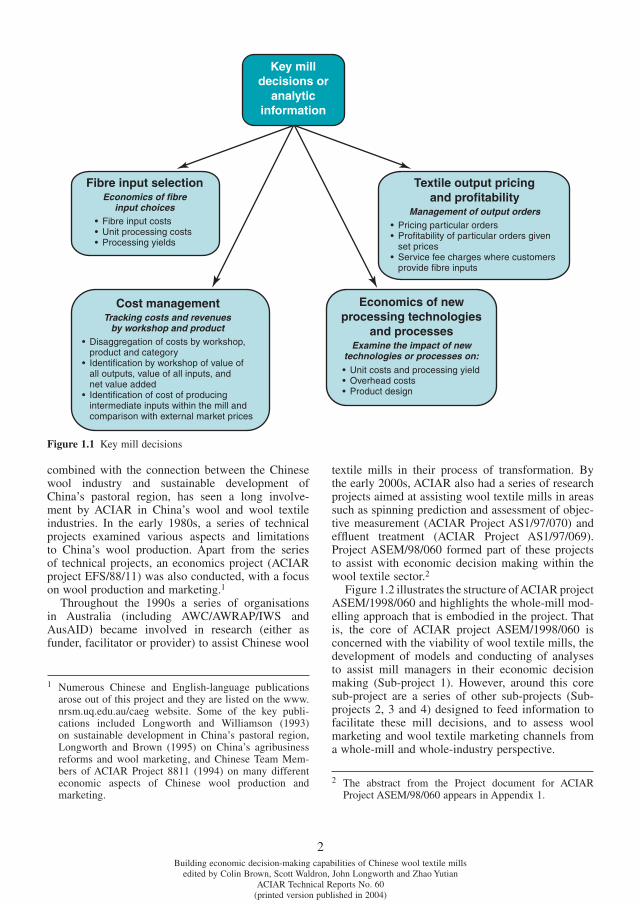
The multi-stage, multi-product nature of the wool textile processing means that managers face a myriad of decisions in trying to successfully guide the opera-tion of wool textile mills. Figure 1.1 outlines some of the key economic decisions that mill managers face and are seeking guidance on how to analyse.
One of the most important sets of decisions relates to output pricing and the determination of the profi t-ability of specifi c orders. Traditionally many Chinese wool textile mills have operated in a ‘passive’ mode
of producing to particular customer orders rather than actively promoting or selling particular products. Even within a passive mode of operation, however, there are a number of key decisions that have to be made. For instance, decisions have to be made about how to price the particular order or, if the customer provides the wool input, what service charge should apply. Where markets set the price, decisions have to be made about whether to process the particular order or process other orders instead, necessitating detailed information about the relative profi tability of the particular order.
Another important set of decisions relate to the choice of fi bre or raw material inputs. That is, there are a number of ways to combine different wools and other fi bres to produce particular wool textile outputs. Fibre inputs can impact on the profi tability of processing a particular order through the direct fi bre input cost as well as impacting on processing or transformation yields and affecting the unit costs of processing.
The tight margins associated with many orders as well as the multi-stage nature of wool tex-tile processing mean that mill managers are also extremely concerned with cost management. In man-aging costs, a detailed breakdown of costs across mill departments or workshops is required along with the costs and revenues generated by specifi c orders. Furthermore, the allocation among workshops and orders must be of the real costs.
As mentioned, there has been enormous pres-sure on Chinese wool textile mills to modernise their operations and upgrade their technology. New tech-nologies and processing equipment usually involve substantial investment. Due diligence and careful economic investigation are required to ensure that the investments are both profi table and feasible.
The decisions highlighted in Figure 1.1 represent only some of the decisions that mill managers con-front. In addition to a raft of technical decisions, the economic decisions mentioned above sit high on the agenda of mill managers both in the importance they attach to them and the challenges faced in devising ways to improve their analytic capabilities in these areas.
1.2 ACIAR involvement and Project ASEM/1998/060
The complementarity between the Chinese wool textile industry and the Australian wool industry,
1
1. Introduction
2Building economic decision-making capabilities of Chinese wool textile mills
edited by Colin Brown, Scott Waldron, John Longworth and Zhao YutianACIAR Technical Reports No. 60
(printed version published in 2004)
combined with the connection between the Chinese wool industry and sustainable development of China’s pastoral region, has seen a long involve-ment by ACIAR in China’s wool and wool textile industries. In the early 1980s, a series of technical projects examined various aspects and limitations to China’s wool production. Apart from the series of technical projects, an economics project (ACIAR project EFS/88/11) was also conducted, with a focus on wool production and marketing.1
Throughout the 1990s a series of organisations in Australia (including AWC/AWRAP/IWS and AusAID) became involved in research (either as funder, facilitator or provider) to assist Chinese wool
textile mills in their process of transformation. By the early 2000s, ACIAR also had a series of research projects aimed at assisting wool textile mills in areas such as spinning prediction and assessment of objec-tive measurement (ACIAR Project AS1/97/070) and effl uent treatment (ACIAR Project AS1/97/069). Project ASEM/98/060 formed part of these projects to assist with economic decision making within the wool textile sector.2
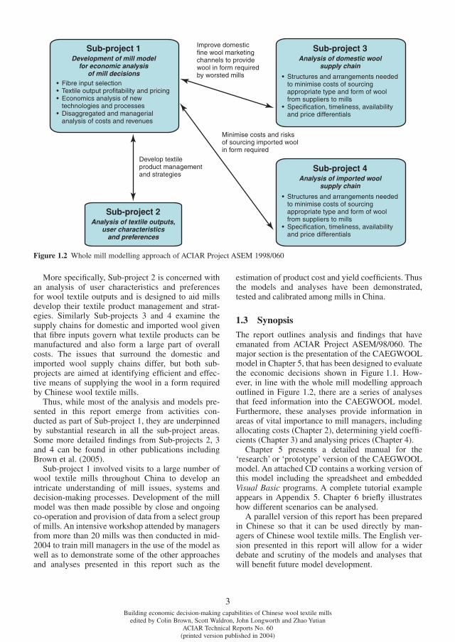
Figure 1.2 illustrates the structure of ACIAR project ASEM/1998/060 and highlights the whole-mill mod-elling approach that is embodied in the project. That is, the core of ACIAR project ASEM/1998/060 is concerned with the viability of wool textile mills, the development of models and conducting of analyses to assist mill managers in their economic decision making (Sub-project 1). However, around this core sub-project are a series of other sub-projects (Sub-projects 2, 3 and 4) designed to feed information to facilitate these mill decisions, and to assess wool marketing and wool textile marketing channels from a whole-mill and whole-industry perspective.
1 Numerous Chinese and English-language publications arose out of this project and they are listed on the www.nrsm.uq.edu.au/caeg website. Some of the key publi-cations included Longworth and Williamson (1993) on sustainable development in China’s pastoral region, Longworth and Brown (1995) on China’s agribusiness reforms and wool marketing, and Chinese Team Mem-bers of ACIAR Project 8811 (1994) on many different economic aspects of Chinese wool production and marketing.
2 The abstract from the Project document for ACIAR Project ASEM/98/060 appears in Appendix 1.
Figure 1.1 Key mill decisions
Building economic decision-making capabilities of Chinese wool textile millsedited by Colin Brown, Scott Waldron, John Longworth and Zhao Yutian
ACIAR Technical Reports No. 60(printed version published in 2004)
More specifi cally, Sub-project 2 is concerned with an analysis of user characteristics and preferences for wool textile outputs and is designed to aid mills develop their textile product management and strat-egies. Similarly Sub-projects 3 and 4 examine the supply chains for domestic and imported wool given that fi bre inputs govern what textile products can be manufactured and also form a large part of overall costs. The issues that surround the domestic and imported wool supply chains differ, but both sub-projects are aimed at identifying effi cient and effec-tive means of supplying the wool in a form required by Chinese wool textile mills.
Thus, while most of the analysis and models pre-sented in this report emerge from activities con-ducted as part of Sub-project 1, they are underpinned by substantial research in all the sub-project areas. Some more detailed fi ndings from Sub-projects 2, 3 and 4 can be found in other publications including Brown et al. (2005).
Sub-project 1 involved visits to a large number of wool textile mills throughout China to develop an intricate understanding of mill issues, systems and decision-making processes. Development of the mill model was then made possible by close and ongoing co-operation and provision of data from a select group of mills. An intensive workshop attended by managers from more than 20 mills was then conducted in mid-2004 to train mill managers in the use of the model as well as to demonstrate some of the other approaches and analyses presented in this report such as the
estimation of product cost and yield coeffi cients. Thus the models and analyses have been demonstrated, tested and calibrated among mills in China.
1.3 Synopsis
The report outlines analysis and fi ndings that have emanated from ACIAR Project ASEM/98/060. The major section is the presentation of the CAEGWOOL model in Chapter 5, that has been designed to evaluate the economic decisions shown in Figure 1.1. How-ever, in line with the whole mill modelling approach outlined in Figure 1.2, there are a series of analyses that feed information into the CAEGWOOL model. Further more, these analyses provide information in areas of vital importance to mill managers, including allocating costs (Chapter 2), determining yield coeffi -cients (Chapter 3) and analysing prices (Chapter 4).
Chapter 5 presents a detailed manual for the ‘research’ or ‘prototype’ version of the CAEGWOOL model. An attached CD contains a working version of this model including the spreadsheet and embedded Visual Basic programs. A complete tutorial example appears in Appendix 5. Chapter 6 briefl y illustrates how different scenarios can be analysed.
A parallel version of this report has been prepared in Chinese so that it can be used directly by man-agers of Chinese wool textile mills. The English ver-sion presented in this report will allow for a wider debate and scrutiny of the models and analyses that will benefi t future model development.
3
Figure 1.2 Whole mill modelling approach of ACIAR Project ASEM 1998/060
4Building economic decision-making capabilities of Chinese wool textile mills
edited by Colin Brown, Scott Waldron, John Longworth and Zhao YutianACIAR Technical Reports No. 60
(printed version published in 2004)
ONE of the most pressing problems perceived by senior mill managers in evaluating new orders or products, or in determining prices for their outputs, is how to allocate costs of manufacturing to partic-ular product orders. Products incur different unit costs of processing for three main reasons. First, characteristics of the product affect the type and level of processing. Second, attributes of the wool input may also require different processing. Third, each product may be associated with a unique yield or physical processing loss that, in turn, will affect the amount of input that has to be processed and so per unit costs.
In summary, different wool inputs and outputs involve different costs to process. Managers are aware of this through anecdotal observations such as extra breakages associated with tender wool requiring additional labour. However, they have little basis for determining the product-specifi c cost variations.
During the planning era, fi xed coeffi cients for par-ticular product types were specifi ed by the Ministry of Textile Industries and applied within the SOE mill
network. However, these coeffi cients were deter-mined many years ago for a different set of prod-ucts and processes. Some mills still use these old cost coeffi cients although they recognise that they are out-of-date. Because of these problems, in many instances, product/order costs are now simply based on per unit costs for all mill throughputs. Presuming that all order types have the same unit costs can lead to signifi cant biases in cost or profi t analysis, as well as in pricing orders.
From the mill manager’s perspective, the problem can be expressed as how to determine cost coeffi -cients to apply to particular products or orders. These coeffi cients would be normalised against standard products (that is, a coeffi cient of 1.08 would indicate that the particular product has unit costs 8% higher than that of a standard product).
The nature of the product cost coeffi cients is that they are highly mill-specifi c. Thus, generalised coef-fi cients based on even a widespread group of mills may be of little relevance. Instead, it is an area where analysis may need to be conducted at an individual
2. Allocating costs accurately
Figure 2.1 Approaches to estimating cost coeffi cients
5Building economic decision-making capabilities of Chinese wool textile mills
edited by Colin Brown, Scott Waldron, John Longworth and Zhao YutianACIAR Technical Reports No. 60
(printed version published in 2004)
enterprise level. Thus, the discussion below focuses on describing the approach rather than on empha-sising specifi c results.
2.1 Broad approaches to estimating cost coeffi cients
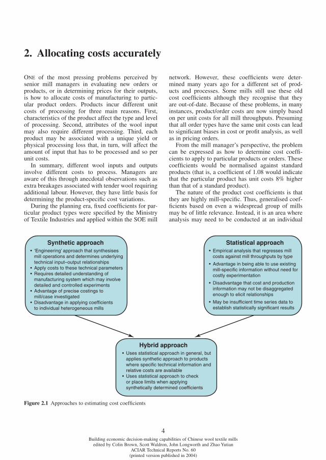
There are two main approaches to the estimation of product-specifi c cost coeffi cients as shown in Figure 2.1. The fi rst of these is an engineering or synthetic approach and the second is a statistical approach. Alternatively, a combination of these approaches involving a hybrid synthetic/statistical approach can be employed.
Both the synthetic and statistical approaches have their merits and shortcomings. The synthetic approach calls for a detailed understanding of the manufacturing system and the underlying technical input-output coeffi cients. Appropriate costing of these technical parameters can reveal precise cost-ings. However, to obtain the necessary technical information requires detailed and controlled experi-ments. Because of the plethora of processes and the complicated nature of wool processing, this requires numerous experiments. In practice, various organi-sations conduct experiments on key processes under selective conditions. That is, the information is spe-cifi c to particular mills, or more precisely, specifi c machines, settings and operational procedures. The advantage of precise costings can be outweighed by the fact that different mills, equipment and set-tings can have a very different set of technical rela-tionships and costings. Given the great heterogeneity in equipment and levels of management in Chinese wool mills, this makes the task of using synthetically determined cost coeffi cients diffi cult to apply to par-ticular mills.
The statistical approach involves the regressing of various cost categories (such as monthly spin-ning labour costs) against various technical informa-tion about the throughputs in that workshop and time period (such as volume or share of pure wool yarn and blended yarn). The approach highlights the fac-tors important in determining unit processing costs and also in the estimation of cost coeffi cients. The statistical approach has the advantage of being mill specifi c and so allowing for technical ineffi ciencies, specifi c mill operating practices, technologies and equipment to be refl ected in the costs. Being able to determine costs to specifi c mills is a major advan-tage given the heterogeneity of wool textile mills. The disadvantage, however, is that the cost and pro-duction information collected by mills may not be in a form that is disaggregated enough to elicit the rela-tionships. Furthermore, there may be an insuffi cient
time series of data to be able to establish statistically signifi cant coeffi cients.
The severe limitations of both the synthetic and statistical approaches suggest that a hybrid synthetic/statistical approach may be required. For instance, tech-nical information may be used to check or place limits on the range of parameter coeffi cient estimates from the statistical analysis and vice versa.
2.2 Statistical approach to estimating cost coeffi cients
Based on the need to develop a relatively straightfor-ward and inexpensive approach that could be used by a wide range of mills to determine cost coeffi cients, the statistical approach was investigated. The fol-lowing sections describe in detail the steps involved in this approach, including the data required.
2.2.1 Method of analysis
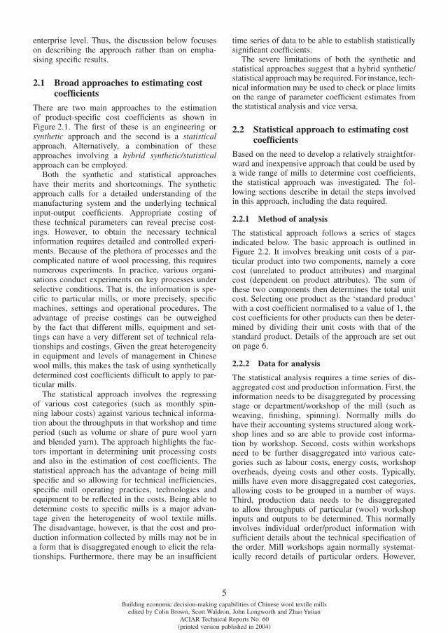
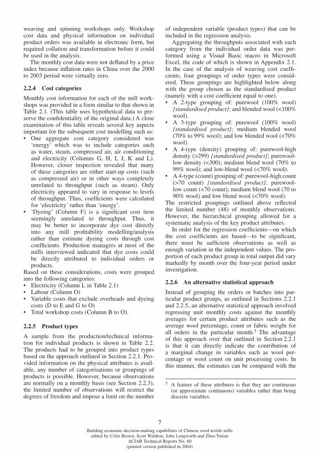
The statistical approach follows a series of stages indicated below. The basic approach is outlined in Figure 2.2. It involves breaking unit costs of a par-ticular product into two components, namely a core cost (unrelated to product attributes) and marginal cost (dependent on product attributes). The sum of these two components then determines the total unit cost. Selecting one product as the ‘standard product’ with a cost coeffi cient normalised to a value of 1, the cost coeffi cients for other products can then be deter-mined by dividing their unit costs with that of the standard product. Details of the approach are set out on page 6.
2.2.2 Data for analysis
The statistical analysis requires a time series of dis-aggregated cost and production information. First, the information needs to be disaggregated by processing stage or department/workshop of the mill (such as weaving, fi nishing, spinning). Normally mills do have their accounting systems structured along work-shop lines and so are able to provide cost informa-tion by workshop. Second, costs within workshops need to be further disaggregated into various cate-gories such as labour costs, energy costs, workshop overheads, dyeing costs and other costs. Typically, mills have even more disaggregated cost categories, allowing costs to be grouped in a number of ways. Third, production data needs to be disaggregated to allow throughputs of particular (wool) workshop inputs and outputs to be determined. This normally involves individual order/product information with suffi cient details about the technical specifi cation of the order. Mill workshops again normally systemat-ically record details of particular orders. However,
6Building economic decision-making capabilities of Chinese wool textile mills
edited by Colin Brown, Scott Waldron, John Longworth and Zhao YutianACIAR Technical Reports No. 60
(printed version published in 2004)
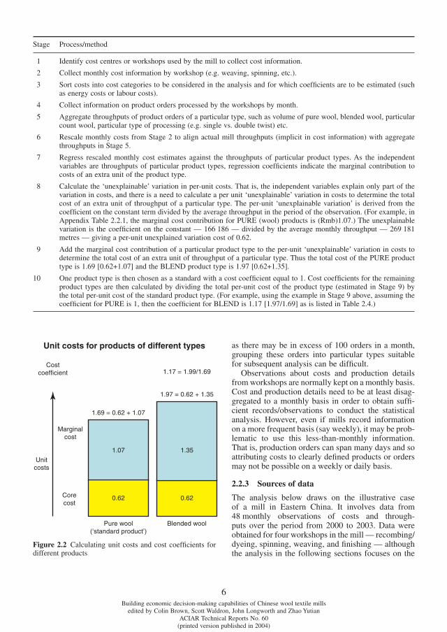
Stage Process/method
1 Identify cost centres or workshops used by the mill to collect cost information.
2 Collect monthly cost information by workshop (e.g. weaving, spinning, etc.).
3 Sort costs into cost categories to be considered in the analysis and for which coeffi cients are to be estimated (such as energy costs or labour costs).
4 Collect information on product orders processed by the workshops by month.
5 Aggregate throughputs of product orders of a particular type, such as volume of pure wool, blended wool, particular count wool, particular type of processing (e.g. single vs. double twist) etc.
6 Rescale monthly costs from Stage 2 to align actual mill throughputs (implicit in cost information) with aggregate throughputs in Stage 5.
7 Regress rescaled monthly cost estimates against the throughputs of particular product types. As the independent variables are throughputs of particular product types, regression coeffi cients indicate the marginal contribution to costs of an extra unit of the product type.
8 Calculate the ‘unexplainable’ variation in per-unit costs. That is, the independent variables explain only part of the variation in costs, and there is a need to calculate a per unit ‘unexplainable’ variation in costs to determine the total cost of an extra unit of throughput of a particular type. The per-unit ‘unexplainable variation’ is derived from the coeffi cient on the constant term divided by the average throughput in the period of the observation. (For example, in Appendix Table 2.2.1, the marginal cost contribution for PURE (wool) products is (Rmb)1.07.) The unexplainable variation is the coeffi cient on the constant — 166 186 — divided by the average monthly throughput — 269 181 metres — giving a per-unit unexplained variation cost of 0.62.
9 Add the marginal cost contribution of a particular product type to the per-unit ‘unexplainable’ variation in costs to determine the total cost of an extra unit of throughput of a particular type. Thus the total cost of the PURE product type is 1.69 [0.62+1.07] and the BLEND product type is 1.97 [0.62+1.35].
10 One product type is then chosen as a standard with a cost coeffi cient equal to 1. Cost coeffi cients for the remaining product types are then calculated by dividing the total per-unit cost of the product type (estimated in Stage 9) by the total per-unit cost of the standard product type. (For example, using the example in Stage 9 above, assuming the coeffi cient for PURE is 1, then the coeffi cient for BLEND is 1.17 [1.97/1.69] as is listed in Table 2.4.)
as there may be in excess of 100 orders in a month, grouping these orders into particular types suitable for subsequent analysis can be diffi cult.
Observations about costs and production details from workshops are normally kept on a monthly basis. Cost and production details need to be at least disag-gregated to a monthly basis in order to obtain suffi -cient records/observations to conduct the statistical analysis. However, even if mills record information on a more frequent basis (say weekly), it may be prob-lematic to use this less-than-monthly information. That is, production orders can span many days and so attributing costs to clearly defi ned products or orders may not be possible on a weekly or daily basis.
2.2.3 Sources of data
The analysis below draws on the illustrative case of a mill in Eastern China. It involves data from 48 monthly observations of costs and through-puts over the period from 2000 to 2003. Data were obtained for four workshops in the mill — recombing/dyeing, spinning, weaving, and fi nishing — although the analysis in the following sections focuses on the
Figure 2.2 Calculating unit costs and cost coeffi cients for different products
7Building economic decision-making capabilities of Chinese wool textile mills
edited by Colin Brown, Scott Waldron, John Longworth and Zhao YutianACIAR Technical Reports No. 60
(printed version published in 2004)
weaving and spinning workshops only. Workshop cost data and physical information on individual product orders was available in electronic form, but required collation and transformation before it could be used in the analysis.
The monthly cost data were not defl ated by a price index because infl ation rates in China over the 2000 to 2003 period were virtually zero.
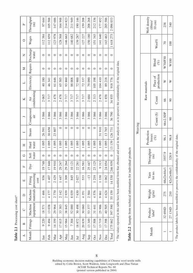
2.2.4 Cost categories
Monthly cost information for each of the mill work-shops was provided in a form similar to that shown in Table 2.1. (This table uses hypothetical data to pre-serve the confi dentiality of the original data.) A close examination of this table reveals several key aspects important for the subsequent cost modelling such as:• One aggregate cost category considered was
‘energy’ which was to include categories such as water, steam, compressed air, air conditioning and electricity (Columns G, H, I, J, K and L). However, closer inspection revealed that many of these categories are either start-up costs (such as compressed air) or in other ways completely unrelated to throughput (such as steam). Only electricity appeared to vary in response to levels of throughput. Thus, coeffi cients were calculated for ‘electricity’ rather than ‘energy’.
• ‘Dyeing’ (Column F) is a signifi cant cost item seemingly unrelated to throughput. Thus, it may be better to incorporate dye cost directly into any mill profi tability modelling/analysis rather than estimate dyeing costs through cost coeffi cients. Production managers at most of the mills interviewed indicated that dye costs could be directly attributed to individual orders or products.
Based on these considerations, costs were grouped into the following categories:• Electricity (Column L in Table 2.1)• Labour (Column O)• Variable costs that exclude overheads and dyeing
costs (D to E and G to O)• Total workshop costs (Column B to O).
2.2.5 Product types
A sample from the production/technical informa-tion for individual products is shown in Table 2.2. The products had to be grouped into product types based on the approach outlined in Section 2.2.1. Pro-vided information on the physical attributes is avail-able, any number of categorisations or groupings of products is possible. However, because observations are normally on a monthly basis (see Section 2.2.3), the limited number of observations will restrict the degrees of freedom and impose a limit on the number
of independent variable (product types) that can be included in the regression analysis.
Aggregating the throughputs associated with each category from the individual order data was per-formed using a Visual Basic macro in Microsoft Excel, the code of which is shown in Appendix 2.1. In the case of the analysis of weaving cost coeffi -cients, four groupings of order types were consid-ered. These groupings are highlighted below along with the group chosen as the standardised product (namely with a cost coeffi cient equal to one).• A 2-type grouping of: purewool (100% wool)
{standardised product}; and blended wool (<100% wool).
• A 3-type grouping of: purewool (100% wool) {standardised product}; medium blended wool (70% to 99% wool); and low blended wool (<70% wool).
• A 4-type (density) grouping of: purewool-high density (>299) {standardised product}; purewool-low density (<300); medium blend wool (70% to 99% wool); and low-blend wool (<70% wool).
• A 4-type (count) grouping of: purewool-high count (>70 count) {standardised product}; purewool-low count (<70 count); medium blend wool (70 to 90% wool) and low blend wool (<70% wool).
The restricted groupings outlined above refl ected the limited number (48) of monthly observations. However, the hierarchical grouping allowed for a systematic analysis of the key product attributes.
In order for the regression coeffi cients—on which the cost coeffi cients are based—to be signifi cant, there must be suffi cient observations as well as enough variation in the independent values. The pro-portion of each product group in total output did vary markedly by month over the four-year period under investigation.
2.2.6 An alternative statistical approach
Instead of grouping the orders or batches into par-ticular product groups, as outlined in Sections 2.2.1 and 2.2.5, an alternative statistical approach involved regressing unit monthly costs against the monthly averages for certain product attributes such as the average wool percentage, count or fabric weight for all orders in the particular month.3 The advantage of this approach over that outlined in Section 2.2.1 is that it can directly indicate the contribution of a marginal change in variables such as wool per-centage or wool count on unit processing costs. In this manner, the estimates can be compared with the
3 A feature of these attributes is that they are continuous (or approximate continuous) variables rather than being discrete variables.
8Building economic decision-making capabilities of Chinese wool textile mills
edited by Colin Brown, Scott Waldron, John Longworth and Zhao YutianACIAR Technical Reports No. 60
(printed version published in 2004)
Tabl
e 2.
1 Pr
oces
sing
cos
t sh
eet*
AB
CD
EF
GH
IJ
KL
MN
OP
Mon
thFi
tting
sM
achi
ne
equi
pmen
tM
achi
ne
mat
eria
lsFi
tting
proc
essi
ng
cost
Dye
Soft
w
ater
Har
d w
ater
Stea
mC
ompr
esse
d ai
rA
ir
cond
ition
ing
Ele
ctri
city
Rep
airs
Dis
char
ge
wat
erW
ages
Thr
ough
put
(m)
Jan
9 22
018
571
1 46
693
619
748
01
095
26 5
913
066
2 06
540
180
00
112
384
97 6
44
Feb
9 49
413
038
4 17
71
407
17 8
480
1 09
530
658
3 06
63
717
46 3
410
011
2 85
910
5 58
8
Mar
14 3
5929
964
2 77
02
429
19 9
100
1 09
523
807
3 06
62
478
61 6
460
012
3 97
814
7 68
6
Apr
17 8
1533
383
2 14
21
447
29 2
470
1 09
50
3 06
62
478
65 5
850
012
8 56
816
4 94
8
May
15 9
8438
845
2 93
91
309
29 2
640
1 09
50
3 06
63
717
93 8
600
014
6 66
321
4 82
3
Jun
7 30
452
000
8 03
984
510
121
01
095
03
066
3 71
788
008
00
140
682
211
949
Jul
18 8
7230
498
7 63
02
027
22 2
810
1 09
50
3 06
63
717
72 9
000
013
9 28
719
0 14
6
Aug
20 8
3930
060
4 35
153
316
581
01
095
03
066
3 71
772
337
00
127
227
159
208
Sep
13 3
4953
377
2 58
4–1
325
447
01
095
03
066
2 68
479
090
00
150
180
208
268
Oct
17 5
0831
441
4 57
61
219
23 1
250
1 09
50
3 06
62
313
105
198
00
151
343
212
336
Nov
13 7
1925
906
9 86
11
330
9 31
30
1 09
531
910
3 06
62
478
104
410
00
141
640
177
852
Dec
17 3
9840
505
4 62
41
062
24 0
540
1 09
513
765
3 06
61
858
89 2
180
014
3 46
320
5 58
6
Tota
l17
5 86
239
7 59
055
159
14 5
3024
6 93
90
13 1
3912
6 73
136
790
34 9
3591
8 77
60
01
618
273
2 09
6 03
3
* T
he v
alue
s re
port
ed i
n th
is t
able
hav
e be
en m
odifi
ed f
rom
tha
t ob
tain
ed a
nd u
sed
in t
he a
naly
sis
so a
s to
pre
serv
e th
e co
nfi d
entia
lity
of t
he o
rigi
nal
data
.
Tabl
e 2.
2 Sa
mpl
e fr
om t
echn
ical
inf
orm
atio
n fo
r in
divi
dual
pro
duct
s
Wea
ving
Mon
thPr
oduc
tla
bel* P
Wei
ght
(g/m
)Y
arn
lot
no.
Thr
ough
put
(m)
Prod
uctio
n lo
sses
(%)
Raw
mat
eria
ls
Wef
t de
nsity
(fi
bre
s/10
cm
)C
ount
(S)
Cou
ntPl
ace
of
prod
uctio
nB
lend
(%)
Woo
l%
132
694
D27
568
s/2×
44s/
135
57.9
96.1
66+
2.5D
P66
WW
70/P
30 7
023
8
127
134
D21
082
s/2×
48s/
132
8.9
96.8
9090
WW
100
100
340
* T
he p
rodu
ct l
abel
s ha
ve b
een
mod
ifi ed
to
pres
erve
the
con
fi den
tialit
y of
the
ori
gina
l da
ta.
9Building economic decision-making capabilities of Chinese wool textile mills
edited by Colin Brown, Scott Waldron, John Longworth and Zhao YutianACIAR Technical Reports No. 60
(printed version published in 2004)
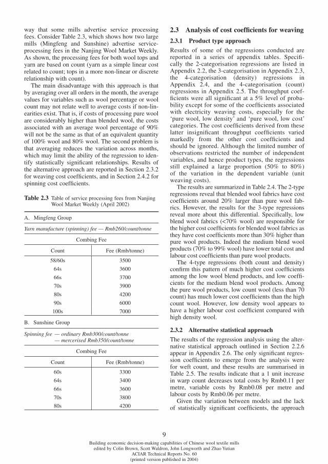
way that some mills advertise service processing fees. Consider Table 2.3, which shows how two large mills (Mingfeng and Sunshine) advertise service-processing fees in the Nanjing Wool Market Weekly. As shown, the processing fees for both wool tops and yarn are based on count (yarn as a simple linear cost related to count; tops in a more non-linear or discrete relationship with count).
The main disadvantage with this approach is that by averaging over all orders in the month, the average values for variables such as wool percentage or wool count may not relate well to average costs if non-lin-earities exist. That is, if costs of processing pure wool are considerably higher than blended wool, the costs associated with an average wool percentage of 90% will not be the same as that of an equivalent quantity of 100% wool and 80% wool. The second problem is that averaging reduces the variation across months, which may limit the ability of the regression to iden-tify statistically signifi cant relationships. Results of the alternative approach are reported in Section 2.3.2 for weaving cost coeffi cients, and in Section 2.4.2 for spinning cost coeffi cients.
2.3 Analysis of cost coeffi cients for weaving
2.3.1 Product type approach
Results of some of the regressions conducted are reported in a series of appendix tables. Specifi -cally the 2-categorisation regressions are listed in Appendix 2.2, the 3-categorisation in Appendix 2.3, the 4-categorisation (density) regressions in Appendix 2.4, and the 4-categorisation (count) regressions in Appendix 2.5. The throughput coef-fi cients were all signifi cant at a 5% level of proba-bility except for some of the coeffi cients associated with electricity weaving costs, especially for the ‘pure wool, low density’ and ‘pure wool, low cost’ categories. The cost coeffi cients derived from these latter insignifi cant throughput coeffi cients varied markedly from the other cost coeffi cients and should be ignored. Although the limited number of observations restricted the number of independent variables, and hence product types, the regressions still explained a large proportion (50% to 80%) of the variation in the dependent variable (unit weaving costs).
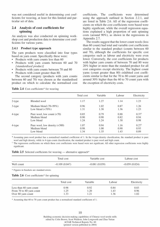
The results are summarized in Table 2.4. The 2-type regressions reveal that blended wool fabrics have cost coeffi cients around 20% larger than pure wool fab-rics. However, the results for the 3-type regressions reveal more about this differential. Specifi cally, low blend wool fabrics (<70% wool) are responsible for the higher cost coeffi cients for blended wool fabrics as they have cost coeffi cients more than 30% higher than pure wool products. Indeed the medium blend wool products (70% to 99% wool) have lower total cost and labour cost coeffi cients than pure wool products.
The 4-type regressions (both count and density) confi rm this pattern of much higher cost coeffi cients among the low wool blend products, and low coeffi -cients for the medium blend wool products. Among the pure wool products, low count wool (less than 70 count) has much lower cost coeffi cients than the high count wool. However, low density wool appears to have a higher labour cost coeffi cient compared with high density wool.
2.3.2 Alternative statistical approach
The results of the regression analysis using the alter-native statistical approach outlined in Section 2.2.6 appear in Appendix 2.6. The only signifi cant regres-sion coeffi cients to emerge from the analy sis were for weft count, and these results are summarised in Table 2.5. The results indicate that a 1 unit increase in warp count decreases total costs by Rmb0.11 per metre, variable costs by Rmb0.08 per metre and labour costs by Rmb0.06 per metre.
Given the variation between models and the lack of statistically signifi cant coeffi cients, the approach
Table 2.3 Table of service processing fees from Nanjing Wool Market Weekly (April 2002)
A. Mingfeng Group
Yarn manufacture (spinning) fee — Rmb260/count/tonne
Combing Fee
Count Fee (Rmb/tonne)
58/60s 3500
64s 3600
66s 3700
70s 3900
80s 4200
90s 6000
100s 7000
B. Sunshine Group
Spinning fee — ordinary Rmb300/count/tonne — mercerised Rmb350/count/tonne
Combing Fee
Count Fee (Rmb/tonne)
60s 3300
64s 3400
66s 3600
70s 3800
80s 4200
10Building economic decision-making capabilities of Chinese wool textile mills
edited by Colin Brown, Scott Waldron, John Longworth and Zhao YutianACIAR Technical Reports No. 60
(printed version published in 2004)
was not considered useful in determining cost coef-fi cients for weaving, at least for this limited and par-ticular set of data.
2.4 Analysis of cost coeffi cients for spinning
An analysis was also conducted on spinning work-shop cost and production data to determine cost coef-fi cients for various yarns.
2.4.1 Product type approach
The yarn products were classifi ed into four types based on yarn count. Specifi cally these were:• Products with yarn counts less than 60• Products with yarn counts between 60 and 70
{standardised product}• Products with yarn counts between 70 and 80 • Products with count greater than 80.
The second category (products with yarn counts between 60 and 70) was chosen as the standardised product on which to calculate the normalised cost
coeffi cients. The coeffi cients were determined using the approach outlined in Section 2.2.1, and are listed in Table 2.6. All of the regression coeffi -cients on which the cost coeffi cients were based were highly signifi cant, while the overall regression equa-tions explained a high proportion of unit spinning costs (around 90%), as shown in the regressions in Appendix 2.7.
The results suggest that the lower count wools (less than 60 count) had total and variable cost coeffi cients similar to the standard product (counts between 60 and 70), although the coeffi cients for specifi c cost categories such as labour and electricity were even lower. Conversely, the cost coeffi cients for products with higher yarn counts of between 70 and 80 were 20% higher or more than the standard product for all cost categories except electricity. The highest count yarns (count greater than 80) exhibited cost coeffi -cients similar to that for the 70 to 80 count yarns and around 30% higher than the 60 to 70 count yarn with the exception of electricity costs.
Table 2.6 Cost coeffi cients* for spinning
Total cost Variable Labour Electricity
Less than 60 yarn count 0.98 0.92 0.84 0.83From 70 to 80 yarn count 1.25 1.20 1.43 0.96Over 80 yarn count 1.33 1.21 1.36 1.02
* Assuming that 60 to 70 yarn count product has a normalized standard coeffi cient of 1.
Table 2.4 Cost coeffi cients* for weaving
Total cost Variable Labour Electricity
2-type Blended wool 1.17 1.27 1.14 1.23
3-type Medium blend (70–99%) 0.96 1.02 0.87 1.26Low blend (<70%) 1.31 1.38 1.36 1.23
4-type Pure wool, low count (<70) 0.85 0.79 0.88 0.37†
Medium blend 0.90 0.90 0.82 0.94Low blend 1.24 1.24 1.30 0.98
4-type Pure wool, low density (<300) 1.07 0.94 1.16 0.27†
Medium blend 0.98 1.00 0.90 0.93Low blend 1.34 1.35 1.43 0.89
* Assuming pure-wool product has a normalised standard coeffi cient of 1. In the 4-type-density classifi cation, the standard product is pure wool and high density, while in 4-type-count classifi cation, the standard product is pure wool and high count.
† The regression coeffi cients on which these cost coeffi cients were based were not signifi cant. All other regression coeffi cients were highly signifi cant.
Table 2.5 Selected coeffi cients for weaving — alternative approach*
Total cost Variable cost Labour cost
Weft count –0.109 (0.047) –0.081 (0.039) –0.059 (0.024)
* Figures in brackets are standard errors.
11Building economic decision-making capabilities of Chinese wool textile mills
edited by Colin Brown, Scott Waldron, John Longworth and Zhao YutianACIAR Technical Reports No. 60
(printed version published in 2004)
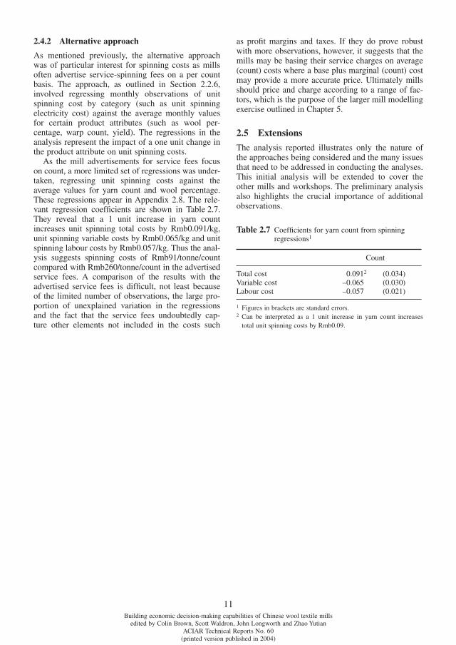
2.4.2 Alternative approach
As mentioned previously, the alternative approach was of particular interest for spinning costs as mills often advertise service-spinning fees on a per count basis. The approach, as outlined in Section 2.2.6, involved regressing monthly observations of unit spinning cost by category (such as unit spinning electricity cost) against the average monthly values for certain product attributes (such as wool per-centage, warp count, yield). The regressions in the analysis represent the impact of a one unit change in the product attribute on unit spinning costs.
As the mill advertisements for service fees focus on count, a more limited set of regressions was under-taken, regressing unit spinning costs against the average values for yarn count and wool percentage. These regressions appear in Appendix 2.8. The rele-vant regression coeffi cients are shown in Table 2.7. They reveal that a 1 unit increase in yarn count increases unit spinning total costs by Rmb0.091/kg, unit spinning variable costs by Rmb0.065/kg and unit spinning labour costs by Rmb0.057/kg. Thus the anal-ysis suggests spinning costs of Rmb91/tonne/count compared with Rmb260/tonne/count in the advertised service fees. A comparison of the results with the advertised service fees is diffi cult, not least because of the limited number of observations, the large pro-portion of unexplained variation in the regressions and the fact that the service fees undoubtedly cap-ture other elements not included in the costs such
as profi t margins and taxes. If they do prove robust with more observations, however, it suggests that the mills may be basing their service charges on average (count) costs where a base plus marginal (count) cost may provide a more accurate price. Ultimately mills should price and charge according to a range of fac-tors, which is the purpose of the larger mill modelling exercise outlined in Chapter 5.
2.5 Extensions
The analysis reported illustrates only the nature of the approaches being considered and the many issues that need to be addressed in conducting the analyses. This initial analysis will be extended to cover the other mills and workshops. The preliminary analysis also highlights the crucial importance of additional observations.
Table 2.7 Coeffi cients for yarn count from spinning regressions1
Count
Total cost 0.0912 (0.034)Variable cost –0.065 (0.030)Labour cost –0.057 (0.021)
1 Figures in brackets are standard errors.2 Can be interpreted as a 1 unit increase in yarn count increases
total unit spinning costs by Rmb0.09.
12Building economic decision-making capabilities of Chinese wool textile mills
edited by Colin Brown, Scott Waldron, John Longworth and Zhao YutianACIAR Technical Reports No. 60
(printed version published in 2004)
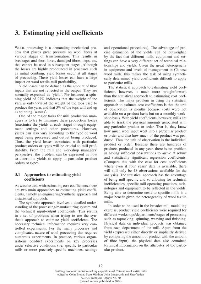
WOOL processing is a demanding mechanical pro-cess that places great pressure on wool fi bres at various stages of transformation. This results in breakages and short fi bres, damaged fi bres, neps, etc, that cannot be used in subsequent stages. Although the losses are highly pronounced in processes such as initial combing, yield losses occur at all stages of processing. These yield losses can have a large impact on wool textile mill profi tability.
Yield losses can be defi ned as the amount of fi bre inputs that are not refl ected in the output. They are normally expressed as ‘yield’. For instance, a spin-ning yield of 97% indicates that the weight of the yarn is only 97% of the weight of the tops used to produce the yarn, and that 3% of the tops will end up as spinning ‘wastes’.
One of the major tasks for mill production man-agers is to try to minimise these production losses (maximise the yields at each stage) through equip-ment settings and other procedures. However, yields can also vary according to the type of wool input being processed and output being produced. Thus, the yield losses associated with particular product orders or types will be crucial to mill prof-itability. From the mill and workshop managers’ pers pective, the problem can be expressed as how to determine yields to apply to particular product orders or types.
3.1 Approaches to estimating yield coeffi cients
As was the case with estimating cost coeffi cients, there are two main approaches to estimating yield coeffi -cients, namely an engineering/synthetic approach and a statistical approach.
The synthetic approach involves a detailed under-standing of the processing/manufacturing system and the technical input-output coeffi cients. This results in a set of problems when trying to use the syn-thetic approach to estimate yield coeffi cients. The necessary technical information requires very con-trolled experiments. For the many processes and complicated nature of wool processing this requires numerous experiments. In practice, various organ-isations conduct experiments on key processes under selective conditions (i.e. specifi c to particular mills or more precisely specifi c machines, settings
and operational procedures). The advantage of pre-cise estimation of the yields can be outweighed by the fact that different mills, equipment and set-tings can have a very different set of technical rela-tionships and yields. Given the great heterogeneity in equipment and levels of management in Chinese wool mills, this makes the task of using syntheti-cally determined yield coeffi cients diffi cult to apply to particular mills.
The statistical approach to estimating yield coef-fi cients, however, is much more straightforward than the statistical approach to estimating cost coef-fi cients. The major problem in using the statistical approach to estimate cost coeffi cients is that the unit of observation is months because costs were not available on a product basis but on a monthly work-shop basis. With yield coeffi cients, however, mills are able to track the physical amounts associated with any particular product or order. That is, they know how much wool input went into a particular product or order and also how much of the product was pro-duced. Thus the unit of observation is the individual product or order. Because there are hundreds of products produced in any year, there is no problem in having suffi cient observations to arrive at robust and statistically signifi cant regression coeffi cients. (Compare this with the case for cost coeffi cients where even if four years’ data is available, there will still only be 48 observations available for the analy sis). The statistical approach has the advantage of being mill specifi c and so allowing for technical ineffi ciencies, specifi c mill operating practices, tech-nologies and equipment to be refl ected in the yields. Being able to determine costs to specifi c mills is a major benefi t given the heterogeneity of wool textile mills.
In order to be used in the broader mill modelling exercise, product yield coeffi cients were required for different workshops/departments/stages of processing such as topmaking, spinning, weaving and fi nishing. Physical data on individual products was obtained from each department of the mill. Apart from the yield (expressed either directly or implicitly derived by comparing the amount of product with the amount of fi bre input), the physical data also contained technical information on the attributes of the partic-ular product.
3. Estimating yield coeffi cients
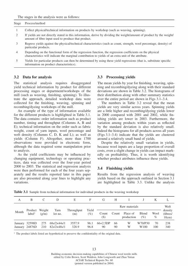
13Building economic decision-making capabilities of Chinese wool textile mills
edited by Colin Brown, Scott Waldron, John Longworth and Zhao YutianACIAR Technical Reports No. 60
(printed version published in 2004)
3.2 Data for analysis
The statistical analysis requires disaggregated yield technical information by product for different processing stages or department/workshops of the mill (such as weaving, fi nishing, spinning). To illus-trate the approach, detailed workshop data were collected for the fi nishing, weaving, spinning and recombing/dyeing workshops of the mill.
An example of the type of information available for the different products is highlighted in Table 3.1. The data contains: order information such as product number, timing and throughput (Columns A, B and E); technical information on the order such as fabric weight, count of yarn inputs, wool percentage and weft density (Columns C, D, K and L); as well as yields (Column F). Altogether, more than 1700 observations were provided in electronic form, although the data required some manipulation prior to analysis.
As the yield coeffi cients may be infl uenced by changing equipment, technology or operating prac-tices, data was collected over the four-year period 2000 to 2003. The statistical and regression analy sis were then performed for each of the four years sep-arately and the results reported later in this paper are also presented along year lines to highlight any variations.
3.3 Processing yields
The mean yields by year for fi nishing, weaving, spin-ning and recombing/dyeing along with their standard deviations are shown in Table 3.2. The histograms of their distribution along with other summary statistics over the entire period are shown in Figs 3.1–3.4.
The numbers in Table 3.2 reveal that the mean yields are very similar across years. Spinning yields are a little higher and recombing/dyeing yields lower in 2000 compared with 2001 and 2002, while fi n-ishing yields are lower in 2003. Furthermore, the varia tion among products within years as refl ected by the standard deviation is also relatively small. Indeed the histograms for all products across all years (Figs 3.1–3.4) indicate that the yields are clustered around a relatively small band of yields.
Despite the relatively small variation in yields, because wool inputs are a large proportion of overall costs, even a slight change in yields can impact mark-edly on profi tability. Thus, it is worth identifying whether product attributes infl uence these yields.
3.4 Finishing yields
Results from the regression analysis of weaving yields based on the approach outlined in Section 3.1 are highlighted in Table 3.3. Unlike the analy sis
The stages in the analysis were as follows:
Stage Process/method
1 Collect physical/technical information on products by workshop (such as weaving, spinning).
2 If yields are not directly stated in this information, derive by dividing the weight/amount of product by the weight/amount of fi bre input used to produce that product.
3 Regress yields against the physical/technical characteristics (such as count, strength, wool percentage, density) of particular products.
4 Depending on the functional form of the regression function, the regression coeffi cients on the physical characteristics will indicate the marginal contribution to yields of an extra unit of the attribute.
5 Yields for particular products can then be determined by using these yield regressions (that is, substitute specifi c information on product characteristics).
Table 3.1 Sample from technical information for individual products in the weaving workshop
A B C D E F G H I J K L
MonthProduct label1
Weight(g/m)
Yarnlot no.
Throughput (m)
Yield(%)
Raw materials Weft density (fi bres/10cm)
Count(S)
Count Place of production
Blend (%)
Wool%
January 32598D 275 68s/2×44s/1 3557.9 96.1 66+2.5DP 66 W W70/P30 70 238January 24876D 210 82s/2×48s/1 328.9 96.8 90 90 W W100 100 340
1 The product labels listed are hypothetical to preserve the confi dentiality of the original data.
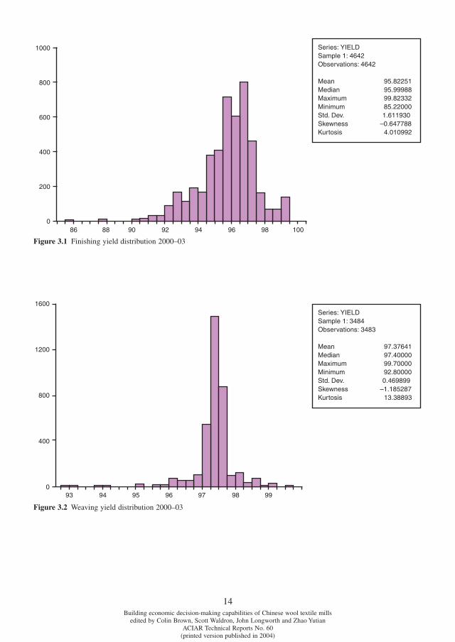
14Building economic decision-making capabilities of Chinese wool textile mills
edited by Colin Brown, Scott Waldron, John Longworth and Zhao YutianACIAR Technical Reports No. 60
(printed version published in 2004)
Figure 3.1 Finishing yield distribution 2000–03
Figure 3.2 Weaving yield distribution 2000–03
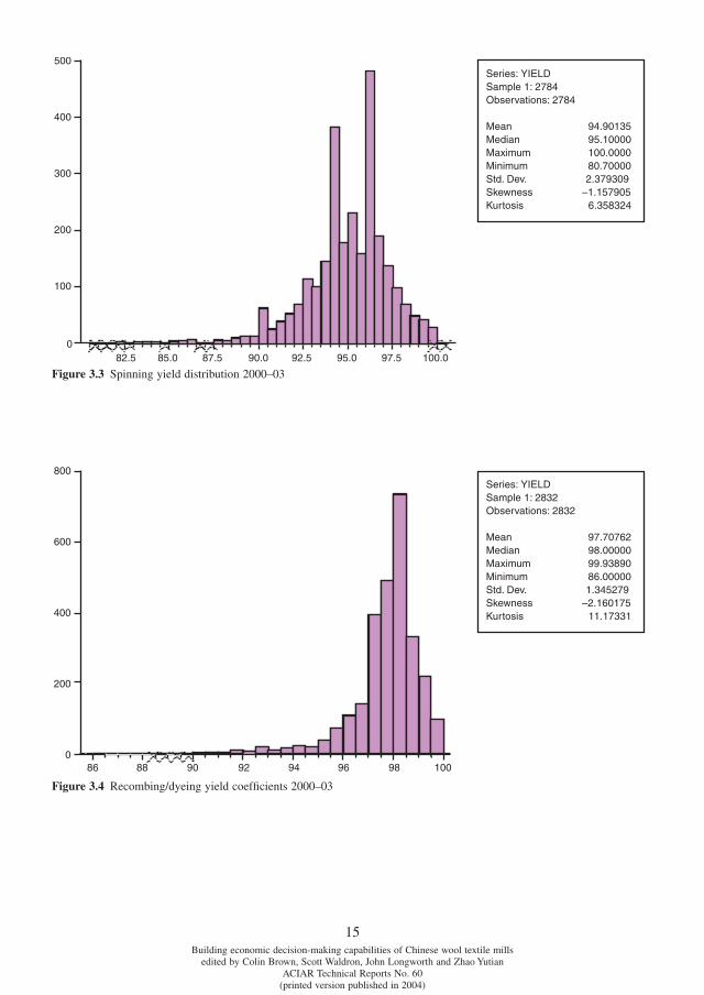
15Building economic decision-making capabilities of Chinese wool textile mills
edited by Colin Brown, Scott Waldron, John Longworth and Zhao YutianACIAR Technical Reports No. 60
(printed version published in 2004)
Figure 3.4 Recombing/dyeing yield coeffi cients 2000–03
Figure 3.3 Spinning yield distribution 2000–03
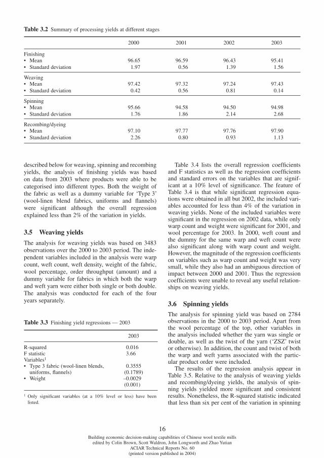
16Building economic decision-making capabilities of Chinese wool textile mills
edited by Colin Brown, Scott Waldron, John Longworth and Zhao YutianACIAR Technical Reports No. 60
(printed version published in 2004)
described below for weaving, spinning and recombing yields, the analysis of fi nishing yields was based on data from 2003 where products were able to be categorised into different types. Both the weight of the fabric as well as a dummy variable for ‘Type 3’ (wool-linen blend fabrics, uniforms and fl annels) were signifi cant although the overall regression explained less than 2% of the variation in yields.
3.5 Weaving yields
The analysis for weaving yields was based on 3483 observations over the 2000 to 2003 period. The inde-pendent variables included in the analysis were warp count, weft count, weft density, weight of the fabric, wool percentage, order throughput (amount) and a dummy variable for fabrics in which both the warp and weft yarn were either both single or both double. The analysis was conducted for each of the four years separately.
Table 3.4 lists the overall regression coeffi cients and F statistics as well as the regression coeffi cients and standard errors on the variables that are signif-icant at a 10% level of signifi cance. The feature of Table 3.4 is that while signifi cant regression equa-tions were obtained in all but 2002, the included vari-ables accounted for less than 4% of the variation in weaving yields. None of the included variables were signifi cant in the regression on 2002 data, while only warp count and weight were signifi cant for 2001, and wool percentage for 2003. In 2000, weft count and the dummy for the same warp and weft count were also signifi cant along with warp count and weight. However, the magnitude of the regression coeffi cients on variables such as warp count and weight was very small, while they also had an ambiguous direction of impact between 2000 and 2001. Thus the regression coeffi cients were unable to reveal any useful relation-ships on weaving yields.
3.6 Spinning yields
The analysis for spinning yield was based on 2784 observations in the 2000 to 2003 period. Apart from the wool percentage of the top, other variables in the analysis included whether the yarn was single or double, as well as the twist of the yarn (‘ZSZ’ twist or otherwise). In addition, the count and twist of both the warp and weft yarns associated with the partic-ular product order were included.
The results of the regression analysis appear in Table 3.5. Relative to the analysis of weaving yields and recombing/dyeing yields, the analysis of spin-ning yields yielded more signifi cant and consistent results. Nonetheless, the R-squared statistic indicated that less than six per cent of the variation in spinning
Table 3.2 Summary of processing yields at different stages
2000 2001 2002 2003
Finishing• Mean 96.65 96.59 96.43 95.41• Standard deviation 1.97 0.56 1.39 1.56
Weaving• Mean 97.42 97.32 97.24 97.43• Standard deviation 0.42 0.56 0.81 0.14
Spinning• Mean 95.66 94.58 94.50 94.98• Standard deviation 1.76 1.86 2.14 2.68
Recombing/dyeing• Mean 97.10 97.77 97.76 97.90• Standard deviation 2.26 0.80 0.93 1.13
Table 3.3 Finishing yield regressions — 2003
2003
R-squared 0.016F statistic 3.66Variables1
• Type 3 fabric (wool-linen blends, uniforms, fl annels)
0.3555(0.1789)
• Weight –0.0029(0.001)
1 Only signifi cant variables (at a 10% level or less) have been listed.
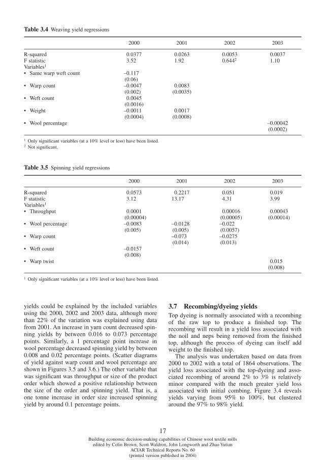
17Building economic decision-making capabilities of Chinese wool textile mills
edited by Colin Brown, Scott Waldron, John Longworth and Zhao YutianACIAR Technical Reports No. 60
(printed version published in 2004)
yields could be explained by the included variables using the 2000, 2002 and 2003 data, although more than 22% of the variation was explained using data from 2001. An increase in yarn count decreased spin-ning yields by between 0.016 to 0.073 percentage points. Similarly, a 1 percentage point increase in wool percentage decreased spinning yield by between 0.008 and 0.02 percentage points. (Scatter diagrams of yield against warp count and wool percentage are shown in Figures 3.5 and 3.6.) The other variable that was signifi cant was throughput or size of the product order which showed a positive relationship between the size of the order and spinning yield. That is, a one tonne increase in order size increased spinning yield by around 0.1 percentage points.
3.7 Recombing/dyeing yieldsTop dyeing is normally associated with a recombing of the raw top to produce a fi nished top. The recombing will result in a yield loss associated with the noil and neps being removed from the fi nished top, although the process of dyeing can itself add weight to the fi nished top.
The analysis was undertaken based on data from 2000 to 2002 with a total of 1864 observations. The yield loss associated with the top-dyeing and asso-ciated recombing of around 2% to 3% is relatively minor compared with the much greater yield loss associated with initial combing. Figure 3.4 reveals yields varying from 95% to 100%, but clustered around the 97% to 98% yield.
Table 3.4 Weaving yield regressions
2000 2001 2002 2003
R-squared 0.0377 0.0263 0.0053 0.0037F statistic 3.52 1.92 0.6442 1.10Variables1
• Same warp weft count –0.117(0.06)
• Warp count –0.0047(0.002)
0.0083(0.0035)
• Weft count 0.0045(0.0016)
• Weight –0.0011(0.0004)
0.0017(0.0008)
• Wool percentage –0.00042(0.0002)
1 Only signifi cant variables (at a 10% level or less) have been listed.2 Not signifi cant.
Table 3.5 Spinning yield regressions
2000 2001 2002 2003
R-squared 0.0573 0.2217 0.051 0.019F statistic 3.12 13.17 4.31 3.99Variables1
• Throughput 0.0001(0.00004)
0.00016(0.00005)
0.00043(0.00014)
• Wool percentage –0.0083(0.005)
–0.0128(0.005)
–0.022(0.0057)
• Warp count –0.073(0.014)
–0.0275(0.013)
• Weft count –0.0157(0.008)
• Warp twist 0.015(0.008)
1 Only signifi cant variables (at a 10% level or less) have been listed.
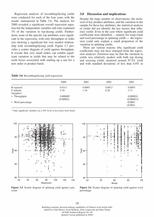
18Building economic decision-making capabilities of Chinese wool textile mills
edited by Colin Brown, Scott Waldron, John Longworth and Zhao YutianACIAR Technical Reports No. 60
(printed version published in 2004)
Regression analyses of recombing/dyeing yields were conducted for each of the four years with the results summarised in Table 3.6. The analysis for 2000 revealed a signifi cant overall regression equa-tion but the independent variables still only explained 3% of the variation in top-dyeing yields. Further-more, none of the specifi c top attributes were signifi -cant in the regression, with only throughput or order size showing a signifi cant but very modest relation-ship with recombing/dyeing yield. Figure 3.7 pro-vides a scatter diagram of yield against throughput. It reveals that very small orders can exhibit signif-icant variation in yields that may be related to the yield losses associated with starting up a run for a new order or product batch.
3.8 Discussion and implications
Despite the large number of observations, the inclu-sion of key product attributes, and the variation in the sample for these key attributes, the statistical analysis of yields did not identify the key factors that infl u-ence yields. Even in the case where signifi cant yield coeffi cients were identifi ed — namely for warp count and wool percentage in spinning yields — the regres-sion could only explain a small proportion of the variation in spinning yields.
There are various reasons why signifi cant yield coeffi cients may not have emerged from the regres-sion analyses. Foremost may be that the variation in yields was relatively modest with both top dyeing and weaving yields clustered around 97.5% yield and with standard deviations of less than 0.8% in
Figure 3.5 Scatter diagram of spinning yield against yarn count
Figure 3.6 Scatter diagram of spinning yield against wool percentage
Table 3.6 Recombing/dyeing yield regressions
2000 2001 2002 2003
R-squared 0.0311 0.0085 0.0012 0.0093F statistic 5.18 1.34 0.28 3.71Variables1
• Throughput 0.000085(0.00002)
0.000024(0.000015)
• Wool percentage –0.0061(0.002)
1 Only signifi cant variables (at a 10% level or less) have been listed.
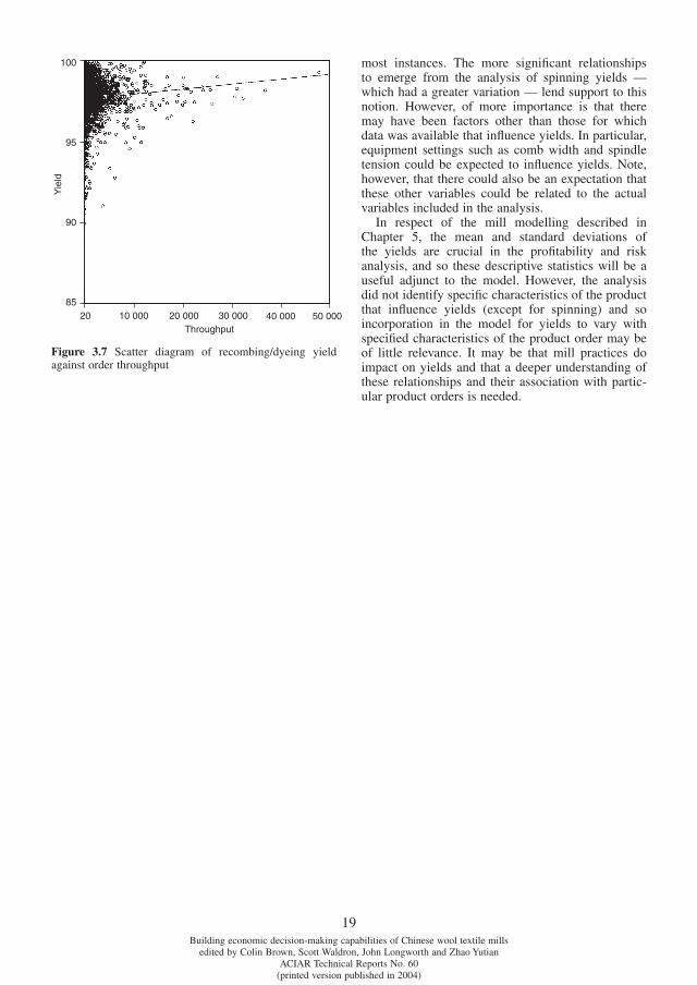
19Building economic decision-making capabilities of Chinese wool textile mills
edited by Colin Brown, Scott Waldron, John Longworth and Zhao YutianACIAR Technical Reports No. 60
(printed version published in 2004)
most instances. The more signifi cant relationships to emerge from the analysis of spinning yields — which had a greater variation — lend support to this notion. However, of more importance is that there may have been factors other than those for which data was available that infl uence yields. In particular, equipment settings such as comb width and spindle tension could be expected to infl uence yields. Note, however, that there could also be an expectation that these other variables could be related to the actual variables included in the analysis.
In respect of the mill modelling described in Chapter 5, the mean and standard deviations of the yields are crucial in the profi tability and risk analy sis, and so these descriptive statistics will be a useful adjunct to the model. However, the analysis did not identify specifi c characteristics of the product that infl uence yields (except for spinning) and so incorporation in the model for yields to vary with specifi ed characteristics of the product order may be of little relevance. It may be that mill practices do impact on yields and that a deeper understanding of these relation ships and their association with partic-ular product orders is needed.
Figure 3.7 Scatter diagram of recombing/dyeing yield against order throughput
20Building economic decision-making capabilities of Chinese wool textile mills
edited by Colin Brown, Scott Waldron, John Longworth and Zhao YutianACIAR Technical Reports No. 60
(printed version published in 2004)
IN ANY investigation of the viability and profitability of Chinese wool textile mills, an analysis of wool and wool textile prices fi gures prominently, either indirectly (in terms of aiding understanding of the incentives of different participants in wool produc-tion, marketing and processing) or directly (such as providing endogenous inputs into the mill model). Figure provides an overview of the various price analyses conducted as part of ACIAR project ASEM/1998/060 in terms of data, methods, outputs and use in the various sub-projects. Specifi cally, the analysis of wool and wool textile prices centred on three main areas of investigation, namely: (a) the determination of the implicit price or value of the attributes that make up wool and wool textile prod-ucts; (b) analysis of the extent of price integration across wool markets in space, time and form dimen-sions; and (c) identifi cation of the extent of seasonal and between-year variation in wool and wool textile prices as well as the general trend in wool prices rel-ative to other fi bre and livestock product prices. Each of these foci is investigated in turn.
4.1 Analysis of the value of wool attributes
Wool and wool textile products are not homoge-neous but comprise many different attributes each of which take on different levels. As user requirements and preferences depend on these attributes, rather than the composite product per se, an analysis of the implicit price or value of these attributes — or the contribution of each of the attributes to the price of the composite product — is worthwhile. Exchange and allocation mechanisms in the past have involved inaccurate pricing systems where many of the implicit prices of the attributes did not refl ect their true values. However, as pressure grows for more accurate prices, both in procuring wool inputs and pricing wool textile outputs, and where increasingly tight profi t margins depend crucially on these fi bre input/textile product choices, an understanding of these premiums and discounts associated with par-ticular input and product characteristics becomes paramount.
The implicit prices associated with product attributes can be obtained through direct questioning or contingent valuation type approaches. However, with some well-defi ned wool markets, the values have also been obtained indirectly using existing market
data through hedonic price type analysis. (See, for example, Angel et al., 1990 for an analysis of Aus-tralian greasy wool prices.) The latter approach — hedonic price analysis — is adopted here.
Because of the range of wool types to be consid-ered in the price analysis, as highlighted in Figure 4.1, market data from a variety of sources was used. The three main sources were:• Analysis of Australian greasy wool prices.
Hedonic price analyses of Australian greasy wool prices are widespread. Indeed, as reported in Section 4.1.1, they have become institutionalised in the price reporting of some agencies. They provide useful and accurate information about the value or implicit price of attributes in Australian greasy wool. Thus, they would be of most use to users purchasing direct from the auctions. However, most greasy wool is purchased in China after passing through a series of intermediaries. Use of these implicit prices presumes that the Law of One Price holds, namely that the prices of Australian greasy wool sold in China follow that of the equivalent wool at the Australian auction. Furthermore, as many mills purchase tops rather than greasy wool, the value of the top attributes rather than the greasy wool attributes will be of importance.
• Analysis of Nanjing Wool Market prices. The Nanjing Wool Market provides what could best be described as a ‘bulletin board’ of offer and bid prices in both print and electronic form. The offer and bid prices do not refl ect negotiated prices and so may bias the implicit prices. Conversely, they do refl ect prices in China after the ‘barrier’ of market traders and other intermediaries.
• Analysis of Chinese auction prices. The Chinese wool auctions are extremely limited as outlined in Brown (1997). However, they provide a more detailed specifi cation of the greasy wool for sale than the Nanjing Wool Market information and involve the wool more closely aligned with Chinese worsted mills. Compared with the analysis of the Australian auction prices, they overcome the issue of the value of the attributes within China. The limited number of observations and ‘contrived’ nature of the auctions limits their usefulness. However, they may be of value in revealing information about the better Chinese wool used in the Chinese worsted wool processing systems.
4. Analysing prices
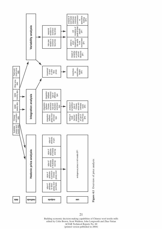
21Building economic decision-making capabilities of Chinese wool textile mills
edited by Colin Brown, Scott Waldron, John Longworth and Zhao YutianACIAR Technical Reports No. 60
(printed version published in 2004)
Fig
ure
4.1
Ove
rvie
w o
f pr
ice
anal
ysis
Hed
on
ic p
rice
an
alys
isIn
teg
rati
on
an
alys
isV
aria
bili
ty a
nal
ysis
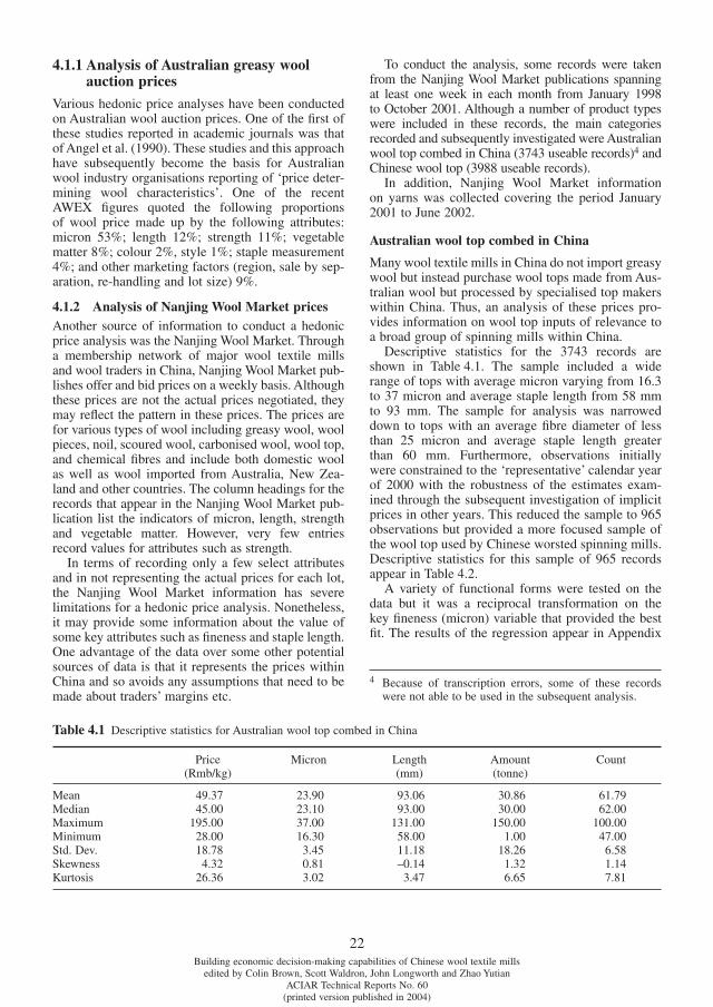
22Building economic decision-making capabilities of Chinese wool textile mills
edited by Colin Brown, Scott Waldron, John Longworth and Zhao YutianACIAR Technical Reports No. 60
(printed version published in 2004)
4.1.1 Analysis of Australian greasy wool auction prices
Various hedonic price analyses have been conducted on Australian wool auction prices. One of the fi rst of these studies reported in academic journals was that of Angel et al. (1990). These studies and this approach have subsequently become the basis for Australian wool industry organisations reporting of ‘price deter-mining wool characteristics’. One of the recent AWEX fi gures quoted the following proportions of wool price made up by the following attributes: micron 53%; length 12%; strength 11%; vegetable matter 8%; colour 2%, style 1%; staple measurement 4%; and other marketing factors (region, sale by sep-aration, re-handling and lot size) 9%.
4.1.2 Analysis of Nanjing Wool Market pricesAnother source of information to conduct a hedonic price analysis was the Nanjing Wool Market. Through a membership network of major wool textile mills and wool traders in China, Nanjing Wool Market pub-lishes offer and bid prices on a weekly basis. Although these prices are not the actual prices negotiated, they may refl ect the pattern in these prices. The prices are for various types of wool including greasy wool, wool pieces, noil, scoured wool, carbonised wool, wool top, and chemical fi bres and include both domestic wool as well as wool imported from Australia, New Zea-land and other countries. The column headings for the records that appear in the Nanjing Wool Market pub-lication list the indicators of micron, length, strength and vegetable matter. However, very few entries record values for attributes such as strength.
In terms of recording only a few select attributes and in not representing the actual prices for each lot, the Nanjing Wool Market information has severe limitations for a hedonic price analysis. Nonetheless, it may provide some information about the value of some key attributes such as fi neness and staple length. One advantage of the data over some other potential sources of data is that it represents the prices within China and so avoids any assumptions that need to be made about traders’ margins etc.
To conduct the analysis, some records were taken from the Nanjing Wool Market publications spanning at least one week in each month from January 1998 to October 2001. Although a number of product types were included in these records, the main cat egories recorded and subsequently investigated were Australian wool top combed in China (3743 useable records)4 and Chinese wool top (3988 useable records).
In addition, Nanjing Wool Market information on yarns was collected covering the period January 2001 to June 2002.
Australian wool top combed in China
Many wool textile mills in China do not import greasy wool but instead purchase wool tops made from Aus-tralian wool but processed by specialised top makers within China. Thus, an analysis of these prices pro-vides information on wool top inputs of relevance to a broad group of spinning mills within China.
Descriptive statistics for the 3743 records are shown in Table 4.1. The sample included a wide range of tops with average micron varying from 16.3 to 37 micron and average staple length from 58 mm to 93 mm. The sample for analysis was narrowed down to tops with an average fi bre diameter of less than 25 micron and average staple length greater than 60 mm. Furthermore, observations initially were constrained to the ‘representative’ calendar year of 2000 with the robustness of the estimates exam-ined through the subsequent investigation of implicit prices in other years. This reduced the sample to 965 observations but provided a more focused sample of the wool top used by Chinese worsted spinning mills. Descriptive statistics for this sample of 965 records appear in Table 4.2.
A variety of functional forms were tested on the data but it was a reciprocal transformation on the key fi neness (micron) variable that provided the best fi t. The results of the regression appear in Appendix
4 Because of transcription errors, some of these records were not able to be used in the subsequent analysis.
Table 4.1 Descriptive statistics for Australian wool top combed in China
Price(Rmb/kg)
Micron Length(mm)
Amount(tonne)
Count
Mean 49.37 23.90 93.06 30.86 61.79Median 45.00 23.10 93.00 30.00 62.00Maximum 195.00 37.00 131.00 150.00 100.00Minimum 28.00 16.30 58.00 1.00 47.00Std. Dev. 18.78 3.45 11.18 18.26 6.58Skewness 4.32 0.81 –0.14 1.32 1.14Kurtosis 26.36 3.02 3.47 6.65 7.81
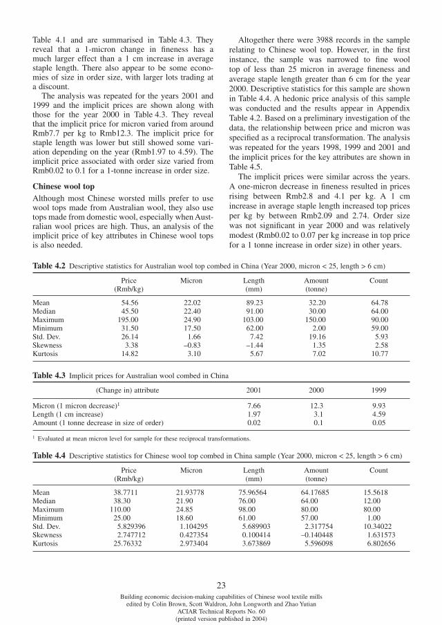
23Building economic decision-making capabilities of Chinese wool textile mills
edited by Colin Brown, Scott Waldron, John Longworth and Zhao YutianACIAR Technical Reports No. 60
(printed version published in 2004)
Table 4.1 and are summarised in Table 4.3. They reveal that a 1-micron change in fi neness has a much larger effect than a 1 cm increase in average staple length. There also appear to be some econo-mies of size in order size, with larger lots trading at a discount.
The analysis was repeated for the years 2001 and 1999 and the implicit prices are shown along with those for the year 2000 in Table 4.3. They reveal that the implicit price for micron varied from around Rmb7.7 per kg to Rmb12.3. The implicit price for staple length was lower but still showed some vari-ation depending on the year (Rmb1.97 to 4.59). The implicit price associated with order size varied from Rmb0.02 to 0.1 for a 1-tonne increase in order size.
Chinese wool topAlthough most Chinese worsted mills prefer to use wool tops made from Australian wool, they also use tops made from domestic wool, especially when Aust-ralian wool prices are high. Thus, an analysis of the implicit price of key attributes in Chinese wool tops is also needed.
Altogether there were 3988 records in the sample relating to Chinese wool top. However, in the fi rst instance, the sample was narrowed to fi ne wool top of less than 25 micron in average fi neness and average staple length greater than 6 cm for the year 2000. Descriptive statistics for this sample are shown in Table 4.4. A hedonic price analysis of this sample was conducted and the results appear in Appendix Table 4.2. Based on a preliminary investigation of the data, the relationship between price and micron was specifi ed as a reciprocal transformation. The analysis was repeated for the years 1998, 1999 and 2001 and the implicit prices for the key attributes are shown in Table 4.5.
The implicit prices were similar across the years. A one-micron decrease in fi neness resulted in prices rising between Rmb2.8 and 4.1 per kg. A 1 cm increase in average staple length increased top prices per kg by between Rmb2.09 and 2.74. Order size was not signifi cant in year 2000 and was relatively modest (Rmb0.02 to 0.07 per kg increase in top price for a 1 tonne increase in order size) in other years.
Table 4.2 Descriptive statistics for Australian wool top combed in China (Year 2000, micron < 25, length > 6 cm)
Price(Rmb/kg)
Micron Length(mm)
Amount(tonne)
Count
Mean 54.56 22.02 89.23 32.20 64.78Median 45.50 22.40 91.00 30.00 64.00Maximum 195.00 24.90 103.00 150.00 90.00Minimum 31.50 17.50 62.00 2.00 59.00Std. Dev. 26.14 1.66 7.42 19.16 5.93Skewness 3.38 –0.83 –1.44 1.35 2.58Kurtosis 14.82 3.10 5.67 7.02 10.77
Table 4.3 Implicit prices for Australian wool combed in China
(Change in) attribute 2001 2000 1999
Micron (1 micron decrease)1 7.66 12.3 9.93Length (1 cm increase) 1.97 3.1 4.59Amount (1 tonne decrease in size of order) 0.02 0.1 0.05
1 Evaluated at mean micron level for sample for these reciprocal transformations.
Table 4.4 Descriptive statistics for Chinese wool top combed in China sample (Year 2000, micron < 25, length > 6 cm)
Price(Rmb/kg)
Micron Length(mm)
Amount(tonne)
Count
Mean 38.7711 21.93778 75.96564 64.17685 15.5618Median 38.30 21.90 76.00 64.00 12.00Maximum 110.00 24.85 98.00 80.00 80.00Minimum 25.00 18.60 61.00 57.00 1.00Std. Dev. 5.829396 1.104295 5.689903 2.317754 10.34022Skewness 2.747712 0.427354 0.100414 –0.140448 1.631573Kurtosis 25.76332 2.973404 3.673869 5.596098 6.802656
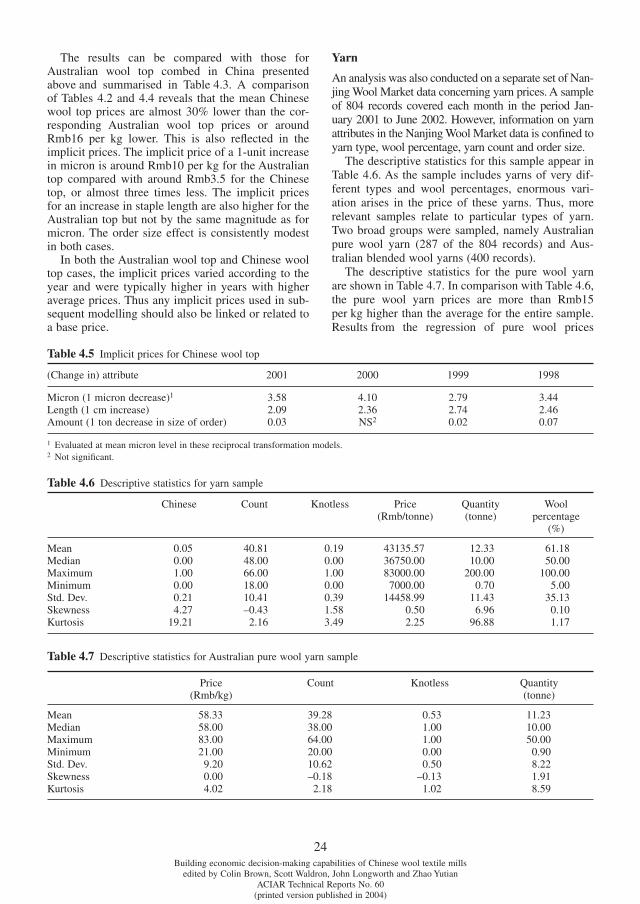
24Building economic decision-making capabilities of Chinese wool textile mills
edited by Colin Brown, Scott Waldron, John Longworth and Zhao YutianACIAR Technical Reports No. 60
(printed version published in 2004)
The results can be compared with those for Australian wool top combed in China presented above and summarised in Table 4.3. A comparison of Tables 4.2 and 4.4 reveals that the mean Chinese wool top prices are almost 30% lower than the cor-responding Australian wool top prices or around Rmb16 per kg lower. This is also refl ected in the implicit prices. The implicit price of a 1-unit increase in micron is around Rmb10 per kg for the Australian top compared with around Rmb3.5 for the Chinese top, or almost three times less. The implicit prices for an increase in staple length are also higher for the Australian top but not by the same magnitude as for micron. The order size effect is consistently modest in both cases.
In both the Australian wool top and Chinese wool top cases, the implicit prices varied according to the year and were typically higher in years with higher average prices. Thus any implicit prices used in sub-sequent modelling should also be linked or related to a base price.
Yarn
An analysis was also conducted on a separate set of Nan-jing Wool Market data concerning yarn prices. A sample of 804 records covered each month in the period Jan-uary 2001 to June 2002. However, information on yarn attributes in the Nanjing Wool Market data is confi ned to yarn type, wool percentage, yarn count and order size.
The descriptive statistics for this sample appear in Table 4.6. As the sample includes yarns of very dif-ferent types and wool percentages, enormous vari-ation arises in the price of these yarns. Thus, more relevant samples relate to particular types of yarn. Two broad groups were sampled, namely Australian pure wool yarn (287 of the 804 records) and Aus-tralian blended wool yarns (400 records).
The descriptive statistics for the pure wool yarn are shown in Table 4.7. In comparison with Table 4.6, the pure wool yarn prices are more than Rmb15 per kg higher than the average for the entire sample. Results from the regression of pure wool prices
Table 4.5 Implicit prices for Chinese wool top
(Change in) attribute 2001 2000 1999 1998
Micron (1 micron decrease)1 3.58 4.10 2.79 3.44Length (1 cm increase) 2.09 2.36 2.74 2.46Amount (1 ton decrease in size of order) 0.03 NS2 0.02 0.07
1 Evaluated at mean micron level in these reciprocal transformation models.2 Not signifi cant.
Table 4.6 Descriptive statistics for yarn sample
Chinese Count Knotless Price(Rmb/tonne)
Quantity(tonne)
Woolpercentage
(%)
Mean 0.05 40.81 0.19 43135.57 12.33 61.18Median 0.00 48.00 0.00 36750.00 10.00 50.00Maximum 1.00 66.00 1.00 83000.00 200.00 100.00Minimum 0.00 18.00 0.00 7000.00 0.70 5.00Std. Dev. 0.21 10.41 0.39 14458.99 11.43 35.13Skewness 4.27 –0.43 1.58 0.50 6.96 0.10Kurtosis 19.21 2.16 3.49 2.25 96.88 1.17
Table 4.7 Descriptive statistics for Australian pure wool yarn sample
Price(Rmb/kg)
Count Knotless Quantity(tonne)
Mean 58.33 39.28 0.53 11.23Median 58.00 38.00 1.00 10.00Maximum 83.00 64.00 1.00 50.00Minimum 21.00 20.00 0.00 0.90Std. Dev. 9.20 10.62 0.50 8.22Skewness 0.00 –0.18 –0.13 1.91Kurtosis 4.02 2.18 1.02 8.59
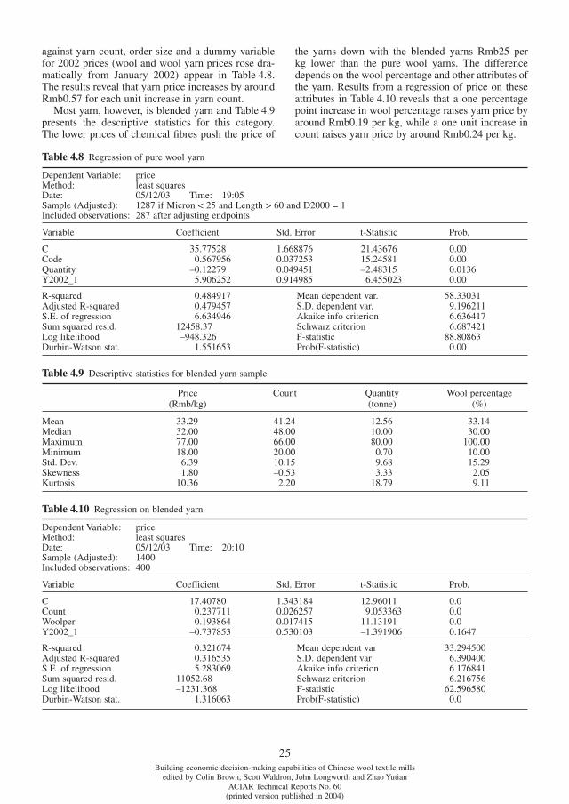
25Building economic decision-making capabilities of Chinese wool textile mills
edited by Colin Brown, Scott Waldron, John Longworth and Zhao YutianACIAR Technical Reports No. 60
(printed version published in 2004)
against yarn count, order size and a dummy variable for 2002 prices (wool and wool yarn prices rose dra-matically from January 2002) appear in Table 4.8. The results reveal that yarn price increases by around Rmb0.57 for each unit increase in yarn count.
Most yarn, however, is blended yarn and Table 4.9 presents the descriptive statistics for this category. The lower prices of chemical fi bres push the price of
the yarns down with the blended yarns Rmb25 per kg lower than the pure wool yarns. The difference depends on the wool percentage and other attributes of the yarn. Results from a regression of price on these attributes in Table 4.10 reveals that a one percentage point increase in wool percentage raises yarn price by around Rmb0.19 per kg, while a one unit increase in count raises yarn price by around Rmb0.24 per kg.
Table 4.8 Regression of pure wool yarn
Dependent Variable: priceMethod: least squaresDate: 05/12/03 Time: 19:05Sample (Adjusted): 1287 if Micron < 25 and Length > 60 and D2000 = 1Included observations: 287 after adjusting endpoints
Variable Coeffi cient Std. Error t-Statistic Prob.
C 35.77528 1.668876 21.43676 0.00Code 0.567956 0.037253 15.24581 0.00Quantity –0.12279 0.049451 –2.48315 0.0136Y2002_1 5.906252 0.914985 6.455023 0.00
R-squared 0.484917 Mean dependent var. 58.33031Adjusted R-squared 0.479457 S.D. dependent var. 9.196211S.E. of regression 6.634946 Akaike info criterion 6.636417Sum squared resid. 12458.37 Schwarz criterion 6.687421Log likelihood –948.326 F-statistic 88.80863Durbin-Watson stat. 1.551653 Prob(F-statistic) 0.00
Table 4.9 Descriptive statistics for blended yarn sample
Price(Rmb/kg)
Count Quantity(tonne)
Wool percentage(%)
Mean 33.29 41.24 12.56 33.14Median 32.00 48.00 10.00 30.00Maximum 77.00 66.00 80.00 100.00Minimum 18.00 20.00 0.70 10.00Std. Dev. 6.39 10.15 9.68 15.29Skewness 1.80 –0.53 3.33 2.05Kurtosis 10.36 2.20 18.79 9.11
Table 4.10 Regression on blended yarn
Dependent Variable: priceMethod: least squaresDate: 05/12/03 Time: 20:10Sample (Adjusted): 1400Included observations: 400
Variable Coeffi cient Std. Error t-Statistic Prob.
C 17.40780 1.343184 12.96011 0.0Count 0.237711 0.026257 9.053363 0.0Woolper 0.193864 0.017415 11.13191 0.0Y2002_1 –0.737853 0.530103 –1.391906 0.1647
R-squared 0.321674 Mean dependent var 33.294500Adjusted R-squared 0.316535 S.D. dependent var 6.390400S.E. of regression 5.283069 Akaike info criterion 6.176841Sum squared resid. 11052.68 Schwarz criterion 6.216756Log likelihood –1231.368 F-statistic 62.596580Durbin-Watson stat. 1.316063 Prob(F-statistic) 0.0
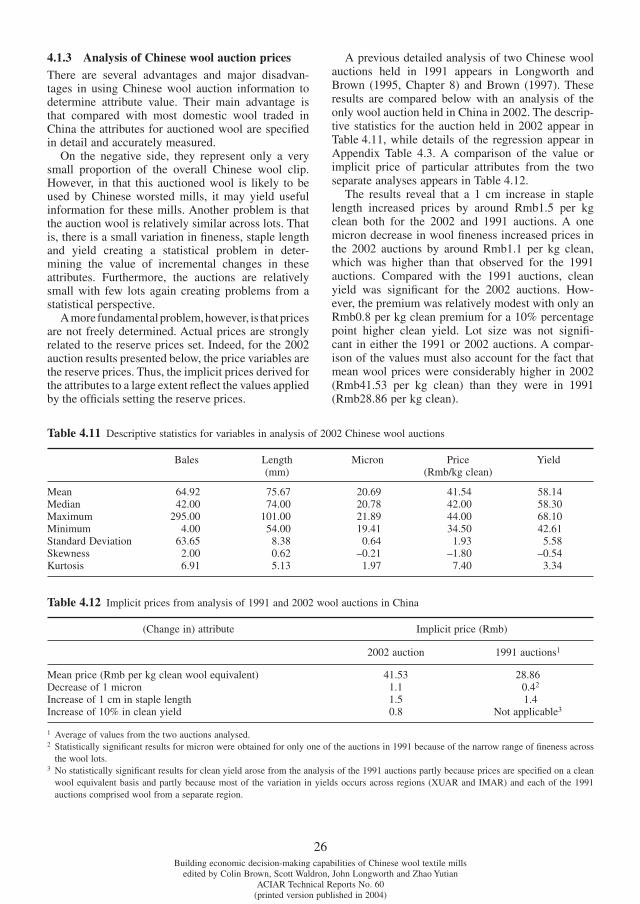
26Building economic decision-making capabilities of Chinese wool textile mills
edited by Colin Brown, Scott Waldron, John Longworth and Zhao YutianACIAR Technical Reports No. 60
(printed version published in 2004)
4.1.3 Analysis of Chinese wool auction pricesThere are several advantages and major disadvan-tages in using Chinese wool auction information to determine attribute value. Their main advantage is that compared with most domestic wool traded in China the attributes for auctioned wool are specifi ed in detail and accurately measured.
On the negative side, they represent only a very small proportion of the overall Chinese wool clip. However, in that this auctioned wool is likely to be used by Chinese worsted mills, it may yield useful information for these mills. Another problem is that the auction wool is relatively similar across lots. That is, there is a small variation in fi neness, staple length and yield creating a statistical problem in deter-mining the value of incremental changes in these attributes. Furthermore, the auctions are relatively small with few lots again creating problems from a statistical perspective.
A more fundamental problem, however, is that prices are not freely determined. Actual prices are strongly related to the reserve prices set. Indeed, for the 2002 auction results presented below, the price variables are the reserve prices. Thus, the implicit prices derived for the attributes to a large extent refl ect the values applied by the offi cials setting the reserve prices.
A previous detailed analysis of two Chinese wool auctions held in 1991 appears in Longworth and Brown (1995, Chapter 8) and Brown (1997). These results are compared below with an analysis of the only wool auction held in China in 2002. The descrip-tive statistics for the auction held in 2002 appear in Table 4.11, while details of the regression appear in Appendix Table 4.3. A comparison of the value or implicit price of particular attributes from the two separate analyses appears in Table 4.12.
The results reveal that a 1 cm increase in staple length increased prices by around Rmb1.5 per kg clean both for the 2002 and 1991 auctions. A one micron decrease in wool fi neness increased prices in the 2002 auctions by around Rmb1.1 per kg clean, which was higher than that observed for the 1991 auctions. Compared with the 1991 auctions, clean yield was signifi cant for the 2002 auctions. How-ever, the premium was relatively modest with only an Rmb0.8 per kg clean premium for a 10% percentage point higher clean yield. Lot size was not signifi -cant in either the 1991 or 2002 auctions. A compar-ison of the values must also account for the fact that mean wool prices were considerably higher in 2002 (Rmb41.53 per kg clean) than they were in 1991 (Rmb28.86 per kg clean).
Table 4.11 Descriptive statistics for variables in analysis of 2002 Chinese wool auctions
Bales Length(mm)
Micron Price(Rmb/kg clean)
Yield
Mean 64.92 75.67 20.69 41.54 58.14Median 42.00 74.00 20.78 42.00 58.30Maximum 295.00 101.00 21.89 44.00 68.10Minimum 4.00 54.00 19.41 34.50 42.61Standard Deviation 63.65 8.38 0.64 1.93 5.58Skewness 2.00 0.62 –0.21 –1.80 –0.54Kurtosis 6.91 5.13 1.97 7.40 3.34
Table 4.12 Implicit prices from analysis of 1991 and 2002 wool auctions in China
(Change in) attribute Implicit price (Rmb)
2002 auction 1991 auctions1
Mean price (Rmb per kg clean wool equivalent) 41.53 28.86Decrease of 1 micron 1.1 0.42
Increase of 1 cm in staple length 1.5 1.4Increase of 10% in clean yield 0.8 Not applicable3
1 Average of values from the two auctions analysed.2 Statistically signifi cant results for micron were obtained for only one of the auctions in 1991 because of the narrow range of fi neness across
the wool lots.3 No statistically signifi cant results for clean yield arose from the analysis of the 1991 auctions partly because prices are specifi ed on a clean
wool equivalent basis and partly because most of the variation in yields occurs across regions (XUAR and IMAR) and each of the 1991 auctions comprised wool from a separate region.
27Building economic decision-making capabilities of Chinese wool textile mills
edited by Colin Brown, Scott Waldron, John Longworth and Zhao YutianACIAR Technical Reports No. 60
(printed version published in 2004)
Ultimately the severe limitations of the analysis using auction data restrict its value in revealing the attribute values. Thus they should be considered only in the light of other information presented in Section 4.1.
4.1.4 Summary of implicit price analysis
Although there is a great volume of information recorded on various wool prices, much of this is in a form not suited to sophisticated implicit price analy sis. Thus the analyses are limited in the extent to which they can reveal the implicit prices or values of attributes, and require careful interpretation given the reliability and nature of the information. Thus, they form only part of the mosaic of determining the implicit price for various wool and wool product attributes.
In terms of linking with mill decision-making models, the results may go some way to endogenising prices rather than rely on externally specifi ed prices. However, to ensure the analysis covers those attributes relevant to the mill, the mill may need to assemble its own data regarding product attributes and prices.
4.2 Market integration
Another area of concern to wool textile mills and to the effi ciency of the industry as a whole is the extent to which the markets for different wool types are integrated. That is, do prices for a particular type of wool or wool top follow the pattern of another type of wool? A preliminary analysis of this integrationwas conducted drawing upon data from the Nanjing Wool Market. From the weekly data that Nanjing Wool Market collects from its network of associate mem-bers (used in the analysis in Section 4.1.2) as well as from external/overseas sources, Nanjing Wool Market collates average prices for selected wool types as well as constructs various price indices. These are again published on a weekly basis in their magazine. Nanjing Wool Market also collates longer time series of these prices on a monthly basis, which are again made avail-able to registered users on their website. The integra-tion analysis was conducted using both the monthly and weekly data.
4.2.1 Monthly price analysis
The monthly price analysis was carried out on monthly data extending from April 1996 to December 2002. To examine some of the integration relationships, seven price series were used. These included the four main types of wool tops used in China, namely Aus-tralian wool combed in China with a count of 60, 64, 66 and 70. Two types of wool tops made from Chinese wool (namely 64- and 66-count) were also
included to examine the extent to which the prices for wool tops made from Chinese wool are related to that from Australian wool. Finally, greasy Australian wool of 66-count was included to determine whether wool top of 66-count followed a similar pattern of prices as that of its corresponding greasy wool input.
The graph of the monthly prices in Figure 4.2 sug-gests that the price series broadly follow the same pattern. The series that appears to move most inde-pendently from the other series is the 70-count Aus-tralian wool top. The series appear to converge towards the latter part of the period.
The correlation matrix in Table 4.13 confi rms the apparent strong correlation between the price series. The particularly strongly correlations are highlighted by the shaded cells in Table 4.13. These include the correlations between the 66-count Australian greasy wool and the Australian 60, 64 and 66 wool tops. Moreover, there is a strong correlation between the Australian 60, 64 and 66 wool top prices. A sim-ilar strong correlation exists between the 60- and 64-count Chinese wool tops. However, none of the other price series (66-count Australian greasy wool, 60- to 66-count Australian wool tops and 64- to 66-count Chinese wool tops) are strongly correlated with the 70-count Australian wool tops.
The pairwise Granger causality tests are shown in Appendix 4 and reveal several relationships. The 66-count Australian wool tops infl uence both 64- and 70-count Australian wool tops. The 64- and 60-count Australian wool tops are closely related, with both appearing to infl uence each other. The 66-count Chinese wool top infl uences 64-count Chinese wool top but not vice versa. However, the pairwise causality tests throw up some less obvious or explainable results such as 64-count Chinese top infl uencing 64-count Australian top, 64-count Australian top infl uencing 70-count Australian top, and 66-count Australian greasy wool infl uencing 70-count Australian wool top.
Some of the correlations observed in Table 4.13 may be spurious and require further co-integration analysis to examine the extent of co-integration of the price series.
4.2.2 Weekly analysis
The price series used in Section 4.2.1 were monthly average prices. However, the process of integration may occur on less than a monthly unit basis. Under these circumstances, using average monthly prices may mask integration among the various price series. To examine the extent of integration in a shorter time frame, weekly data for the period January 2000 to June 2002 were used. The analysis also enabled other price series to be examined as part of the co- integration analysis, including Uruguay greasy wool and Aus-tralian 80-count wool top.
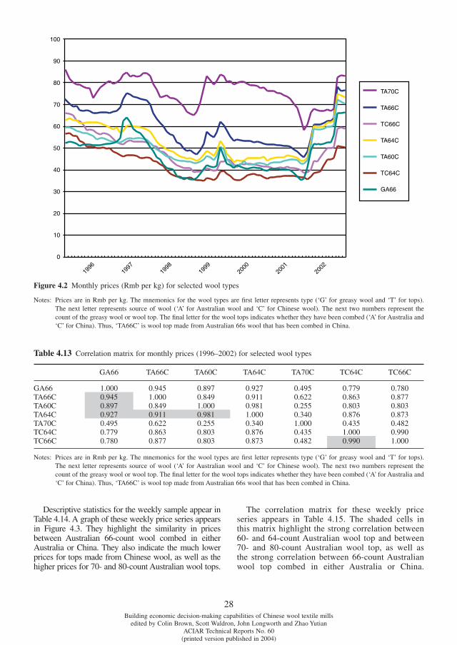
28Building economic decision-making capabilities of Chinese wool textile mills
edited by Colin Brown, Scott Waldron, John Longworth and Zhao YutianACIAR Technical Reports No. 60
(printed version published in 2004)
Descriptive statistics for the weekly sample appear in Table 4.14. A graph of these weekly price series appears in Figure 4.3. They highlight the similarity in prices between Australian 66-count wool combed in either Australia or China. They also indicate the much lower prices for tops made from Chinese wool, as well as the higher prices for 70- and 80-count Australian wool tops.
The correlation matrix for these weekly price series appears in Table 4.15. The shaded cells in this matrix highlight the strong correlation between 60- and 64-count Australian wool top and between 70- and 80-count Australian wool top, as well as the strong correlation between 66-count Australian wool top combed in either Australia or China.
Figure 4.2 Monthly prices (Rmb per kg) for selected wool types
Notes: Prices are in Rmb per kg. The mnemonics for the wool types are fi rst letter represents type (‘G’ for greasy wool and ‘T’ for tops). The next letter represents source of wool (‘A’ for Australian wool and ‘C’ for Chinese wool). The next two numbers represent the count of the greasy wool or wool top. The fi nal letter for the wool tops indicates whether they have been combed (‘A’ for Australia and ‘C’ for China). Thus, ‘TA66C’ is wool top made from Australian 66s wool that has been combed in China.
Table 4.13 Correlation matrix for monthly prices (1996–2002) for selected wool types
GA66 TA66C TA60C TA64C TA70C TC64C TC66C
GA66 1.000 0.945 0.897 0.927 0.495 0.779 0.780TA66C 0.945 1.000 0.849 0.911 0.622 0.863 0.877TA60C 0.897 0.849 1.000 0.981 0.255 0.803 0.803TA64C 0.927 0.911 0.981 1.000 0.340 0.876 0.873TA70C 0.495 0.622 0.255 0.340 1.000 0.435 0.482TC64C 0.779 0.863 0.803 0.876 0.435 1.000 0.990TC66C 0.780 0.877 0.803 0.873 0.482 0.990 1.000
Notes: Prices are in Rmb per kg. The mnemonics for the wool types are fi rst letter represents type (‘G’ for greasy wool and ‘T’ for tops). The next letter represents source of wool (‘A’ for Australian wool and ‘C’ for Chinese wool). The next two numbers represent the count of the greasy wool or wool top. The fi nal letter for the wool tops indicates whether they have been combed (‘A’ for Australia and ‘C’ for China). Thus, ‘TA66C’ is wool top made from Australian 66s wool that has been combed in China.
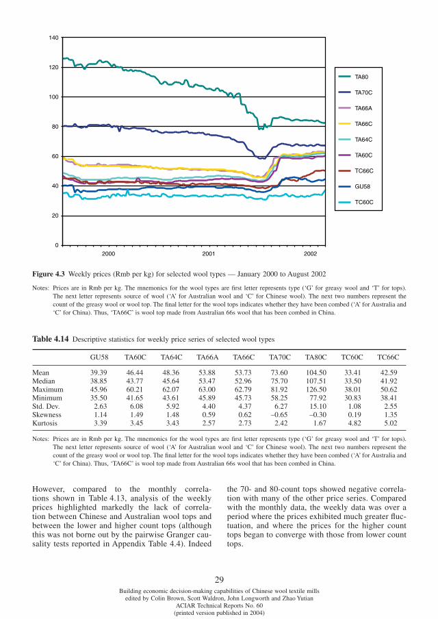
29Building economic decision-making capabilities of Chinese wool textile mills
edited by Colin Brown, Scott Waldron, John Longworth and Zhao YutianACIAR Technical Reports No. 60
(printed version published in 2004)
Figure 4.3 Weekly prices (Rmb per kg) for selected wool types — January 2000 to August 2002
Notes: Prices are in Rmb per kg. The mnemonics for the wool types are fi rst letter represents type (‘G’ for greasy wool and ‘T’ for tops). The next letter represents source of wool (‘A’ for Australian wool and ‘C’ for Chinese wool). The next two numbers represent the count of the greasy wool or wool top. The fi nal letter for the wool tops indicates whether they have been combed (‘A’ for Australia and ‘C’ for China). Thus, ‘TA66C’ is wool top made from Australian 66s wool that has been combed in China.
Table 4.14 Descriptive statistics for weekly price series of selected wool types
GU58 TA60C TA64C TA66A TA66C TA70C TA80C TC60C TC66C
Mean 39.39 46.44 48.36 53.88 53.73 73.60 104.50 33.41 42.59Median 38.85 43.77 45.64 53.47 52.96 75.70 107.51 33.50 41.92Maximum 45.96 60.21 62.07 63.00 62.79 81.92 126.50 38.01 50.62Minimum 35.50 41.65 43.61 45.89 45.73 58.25 77.92 30.83 38.41Std. Dev. 2.63 6.08 5.92 4.40 4.37 6.27 15.10 1.08 2.55Skewness 1.14 1.49 1.48 0.59 0.62 –0.65 –0.30 0.19 1.35Kurtosis 3.39 3.45 3.43 2.57 2.73 2.42 1.67 4.82 5.02
Notes: Prices are in Rmb per kg. The mnemonics for the wool types are fi rst letter represents type (‘G’ for greasy wool and ‘T’ for tops). The next letter represents source of wool (‘A’ for Australian wool and ‘C’ for Chinese wool). The next two numbers represent the count of the greasy wool or wool top. The fi nal letter for the wool tops indicates whether they have been combed (‘A’ for Australia and ‘C’ for China). Thus, ‘TA66C’ is wool top made from Australian 66s wool that has been combed in China.
However, compared to the monthly correla-tions shown in Table 4.13, analysis of the weekly prices highlighted markedly the lack of correla-tion between Chinese and Australian wool tops and between the lower and higher count tops (although this was not borne out by the pairwise Granger cau-sality tests reported in Appendix Table 4.4). Indeed
the 70- and 80-count tops showed negative correla-tion with many of the other price series. Compared with the monthly data, the weekly data was over a period where the prices exhibited much greater fl uc-tuation, and where the prices for the higher count tops began to converge with those from lower count tops.
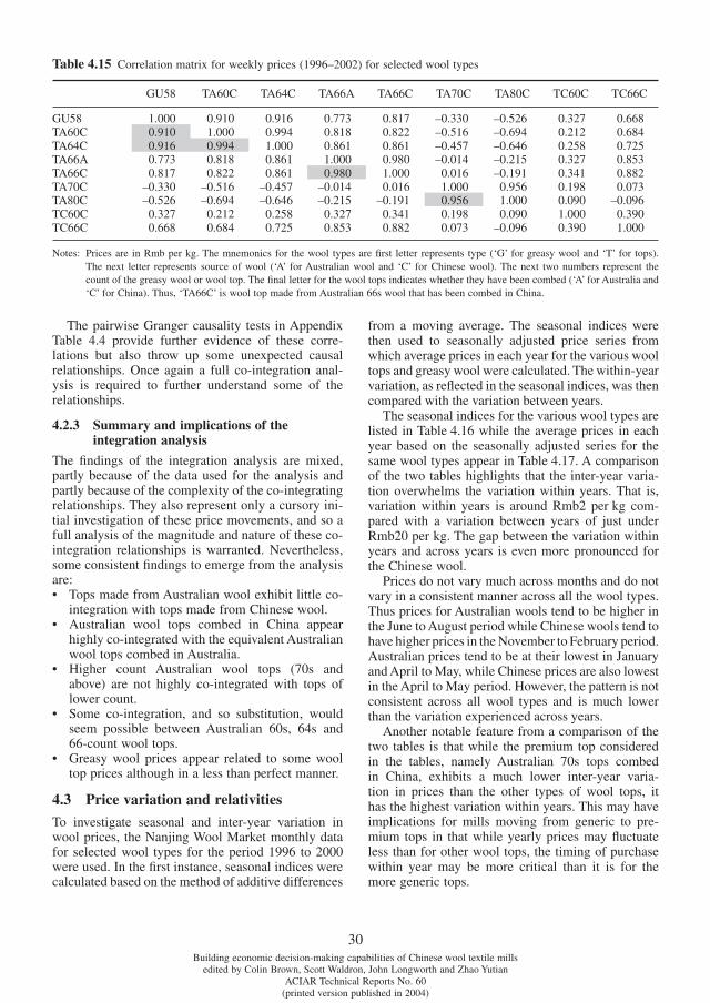
30Building economic decision-making capabilities of Chinese wool textile mills
edited by Colin Brown, Scott Waldron, John Longworth and Zhao YutianACIAR Technical Reports No. 60
(printed version published in 2004)
The pairwise Granger causality tests in Appendix Table 4.4 provide further evidence of these corre-lations but also throw up some unexpected causal relationships. Once again a full co-integration anal-ysis is required to further understand some of the relationships.
4.2.3 Summary and implications of the integration analysis
The fi ndings of the integration analysis are mixed, partly because of the data used for the analysis and partly because of the complexity of the co-integrating relationships. They also represent only a cursory ini-tial investigation of these price movements, and so a full analysis of the magnitude and nature of these co-integration relationships is warranted. Nevertheless, some consistent fi ndings to emerge from the analysis are:• Tops made from Australian wool exhibit little co-
integration with tops made from Chinese wool.• Australian wool tops combed in China appear
highly co-integrated with the equivalent Australian wool tops combed in Australia.
• Higher count Australian wool tops (70s and above) are not highly co-integrated with tops of lower count.
• Some co-integration, and so substitution, would seem possible between Australian 60s, 64s and 66-count wool tops.
• Greasy wool prices appear related to some wool top prices although in a less than perfect manner.
4.3 Price variation and relativities
To investigate seasonal and inter-year variation in wool prices, the Nanjing Wool Market monthly data for selected wool types for the period 1996 to 2000 were used. In the fi rst instance, seasonal indices were calculated based on the method of additive differences
from a moving average. The seasonal indices were then used to seasonally adjusted price series from which average prices in each year for the various wool tops and greasy wool were calculated. The within-year variation, as refl ected in the seasonal indices, was then compared with the variation between years.
The seasonal indices for the various wool types are listed in Table 4.16 while the average prices in each year based on the seasonally adjusted series for the same wool types appear in Table 4.17. A comparison of the two tables highlights that the inter-year varia-tion overwhelms the variation within years. That is, variation within years is around Rmb2 per kg com-pared with a variation between years of just under Rmb20 per kg. The gap between the variation within years and across years is even more pronounced for the Chinese wool.
Prices do not vary much across months and do not vary in a consistent manner across all the wool types. Thus prices for Australian wools tend to be higher in the June to August period while Chinese wools tend to have higher prices in the November to February period. Australian prices tend to be at their lowest in January and April to May, while Chinese prices are also lowest in the April to May period. However, the pattern is not consistent across all wool types and is much lower than the variation experienced across years.
Another notable feature from a comparison of the two tables is that while the premium top considered in the tables, namely Australian 70s tops combed in China, exhibits a much lower inter-year varia-tion in prices than the other types of wool tops, it has the highest variation within years. This may have implications for mills moving from generic to pre-mium tops in that while yearly prices may fl uctuate less than for other wool tops, the timing of purchase within year may be more critical than it is for the more generic tops.
Table 4.15 Correlation matrix for weekly prices (1996–2002) for selected wool types
GU58 TA60C TA64C TA66A TA66C TA70C TA80C TC60C TC66C
GU58 1.000 0.910 0.916 0.773 0.817 –0.330 –0.526 0.327 0.668TA60C 0.910 1.000 0.994 0.818 0.822 –0.516 –0.694 0.212 0.684TA64C 0.916 0.994 1.000 0.861 0.861 –0.457 –0.646 0.258 0.725TA66A 0.773 0.818 0.861 1.000 0.980 –0.014 –0.215 0.327 0.853TA66C 0.817 0.822 0.861 0.980 1.000 0.016 –0.191 0.341 0.882TA70C –0.330 –0.516 –0.457 –0.014 0.016 1.000 0.956 0.198 0.073TA80C –0.526 –0.694 –0.646 –0.215 –0.191 0.956 1.000 0.090 –0.096TC60C 0.327 0.212 0.258 0.327 0.341 0.198 0.090 1.000 0.390TC66C 0.668 0.684 0.725 0.853 0.882 0.073 –0.096 0.390 1.000
Notes: Prices are in Rmb per kg. The mnemonics for the wool types are fi rst letter represents type (‘G’ for greasy wool and ‘T’ for tops). The next letter represents source of wool (‘A’ for Australian wool and ‘C’ for Chinese wool). The next two numbers represent the count of the greasy wool or wool top. The fi nal letter for the wool tops indicates whether they have been combed (‘A’ for Australia and ‘C’ for China). Thus, ‘TA66C’ is wool top made from Australian 66s wool that has been combed in China.
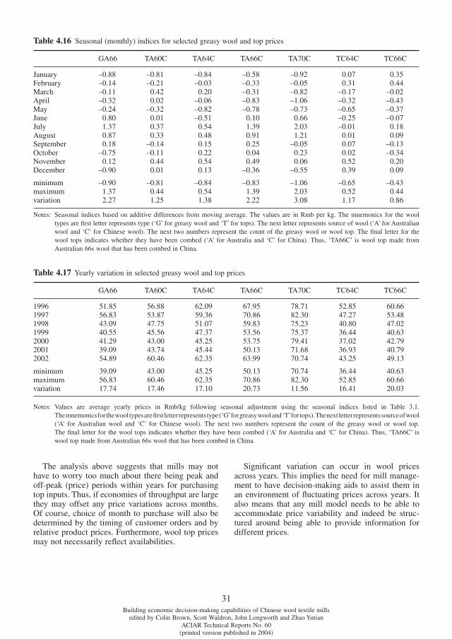
31Building economic decision-making capabilities of Chinese wool textile mills
edited by Colin Brown, Scott Waldron, John Longworth and Zhao YutianACIAR Technical Reports No. 60
(printed version published in 2004)
Table 4.16 Seasonal (monthly) indices for selected greasy wool and top prices
GA66 TA60C TA64C TA66C TA70C TC64C TC66C
January –0.88 –0.81 –0.84 –0.58 –0.92 0.07 0.35February –0.14 –0.21 –0.03 –0.33 –0.05 0.31 0.44March –0.11 0.42 0.20 –0.31 –0.82 –0.17 –0.02April –0.32 0.02 –0.06 –0.83 –1.06 –0.32 –0.43May –0.24 –0.32 –0.82 –0.78 –0.73 –0.65 –0.37June 0.80 0.01 –0.51 0.10 0.66 –0.25 –0.07July 1.37 0.37 0.54 1.39 2.03 –0.01 0.18August 0.87 0.33 0.48 0.91 1.21 0.01 0.09September 0.18 –0.14 0.15 0.25 –0.05 0.07 –0.13October –0.75 –0.11 0.22 0.04 0.23 0.02 –0.34November 0.12 0.44 0.54 0.49 0.06 0.52 0.20December –0.90 0.01 0.13 –0.36 –0.55 0.39 0.09
minimum –0.90 –0.81 –0.84 –0.83 –1.06 –0.65 –0.43maximum 1.37 0.44 0.54 1.39 2.03 0.52 0.44variation 2.27 1.25 1.38 2.22 3.08 1.17 0.86
Notes: Seasonal indices based on additive differences from moving average. The values are in Rmb per kg. The mnemonics for the wool types are fi rst letter represents type (‘G’ for greasy wool and ‘T’ for tops). The next letter represents source of wool (‘A’ for Australian wool and ‘C’ for Chinese wool). The next two numbers represent the count of the greasy wool or wool top. The fi nal letter for the wool tops indicates whether they have been combed (‘A’ for Australia and ‘C’ for China). Thus, ‘TA66C’ is wool top made from Australian 66s wool that has been combed in China.
Table 4.17 Yearly variation in selected greasy wool and top prices
GA66 TA60C TA64C TA66C TA70C TC64C TC66C
1996 51.85 56.88 62.09 67.95 78.71 52.85 60.661997 56.83 53.87 59.36 70.86 82.30 47.27 53.481998 43.09 47.75 51.07 59.83 75.23 40.80 47.021999 40.55 45.56 47.37 53.56 75.37 36.44 40.632000 41.29 43.00 45.25 53.75 79.41 37.02 42.792001 39.09 43.74 45.44 50.13 71.68 36.93 40.792002 54.89 60.46 62.35 63.99 70.74 43.25 49.13
minimum 39.09 43.00 45.25 50.13 70.74 36.44 40.63maximum 56.83 60.46 62.35 70.86 82.30 52.85 60.66variation 17.74 17.46 17.10 20.73 11.56 16.41 20.03
Notes: Values are average yearly prices in Rmb/kg following seasonal adjustment using the seasonal indices listed in Table 3.1.The mnemonics for the wool types are fi rst letter represents type (‘G’ for greasy wool and ‘T’ for tops). The next letter represents source of wool(‘A’ for Australian wool and ‘C’ for Chinese wool). The next two numbers represent the count of the greasy wool or wool top.The fi nal letter for the wool tops indicates whether they have been combed (‘A’ for Australia and ‘C’ for China). Thus, ‘TA66C’ is wool top made from Australian 66s wool that has been combed in China.
The analysis above suggests that mills may not have to worry too much about there being peak and off-peak (price) periods within years for purchasing top inputs. Thus, if economies of throughput are large they may offset any price variations across months. Of course, choice of month to purchase will also be determined by the timing of customer orders and by relative product prices. Furthermore, wool top prices may not necessarily refl ect availabilities.
Signifi cant variation can occur in wool prices across years. This implies the need for mill manage-ment to have decision-making aids to assist them in an environment of fl uctuating prices across years. It also means that any mill model needs to be able to accommodate price variability and indeed be struc-tured around being able to provide information for different prices.
32Building economic decision-making capabilities of Chinese wool textile mills
edited by Colin Brown, Scott Waldron, John Longworth and Zhao YutianACIAR Technical Reports No. 60
(printed version published in 2004)
CAEGWOOL is a Visual Basic model embedded in a Microsoft Excel spreadsheet that is designed to assist decision making by mill managers and tech-nicians in their managerial accounting and economic evaluation of a wide variety of mill decisions. The model has been developed by researchers from the China Agricultural Economics Group at the Univer-sity of Queensland and the Chinese Research Centre for Rural Economy in close association with mill managers and technicians from various Chinese wool textile mills and organisations.
This chapter presents a manual to running the model while Appendix 5 provides a simple tutorial example. The manual is divided into three parts. In this fi rst part — Sections 5.1 and 5.2 — a background to the model, the philosophy behind the model and computer pro-grams, the structure of the model, and key parameters and assumptions in the model are described. Readers interested in instructions on how to run the model and how to interpret its output should proceed direct to Part B — Sections 5.3 to 5.7 — of the manual. The third part of the manual — Part C (Sections 5.8 and 5.9) — describes the Visual Basic code and the various endogenous parameters in the mode. Reference to this part of the manual is not required for normal usage of the model, but will be of use for more advanced usage or for further model development.
Part A — Overview of the Model(Sections 5.1 and 5.2)
This part of the manual provides a background to the model, the philosophy behind the model and computer programs, the structure of the model, and key parameters and assumptions in the model. Users interested in following instructions to run the model can move direct to Part B.
5.1 Introduction
The model was developed as part of ACIAR Project ASEM/1998/060 on ‘An economic analysis of fi bre input/textile product selection and new processing technologies in Chinese wool textile mills’. One part of this project was the development of a whole mill model which could determine the cost and revenue effects of various fi bre input/textile product selec-tions as well as evaluate the cost and revenue effects
of new processing technologies. The project com-menced in 2001 when a detailed understanding of existing mill information and (managerial and fi nan-cial) accounting systems was obtained along with shortcomings in the system identifi ed by mill man-agers. In 2002, close collaboration was conducted with technicians and managers from a select group of mills to collect detailed data and ideas for develop-ment of the model. The model was validated in 2003 with the select group of mills. A larger group of mills received training in the use of the model in 2004.
The initial focus of the project was on develop-ment of a model which could analyse fi bre input/textile product selection and new processing technol-ogies. However, the model developed is much broader and is now able to evaluate the economic impact of many other aspects and decisions that impact on mill revenues and costs. The initial phase of the project identifi ed that while many mills devote considerable effort to collecting detailed (and reliable) informa-tion, they do not make full use of it in management decisions. This was apparent in 2002 when imported wool prices rose by almost 30% and many mill man-agers had little information to assist them respond to the volatile input prices.
5.1.1 Model philosophy
Given this background, the intent was to develop a model that is useful to many Chinese wool textile mills, and that could assist managers and technicians with their management decisions. A key aspect of the approach was that the model would draw on existing sources of mill information and could evolve from existing mill decision-making approaches.
32
5. CAEGWOOL5
5 The version of the model reported in this manual is not a commercial model but a research model. Although exten-sive testing has taken place and every effort has been made to ensure the accuracy of the model, no guarantees can be made that it is free of all errors. Thus users should exercise due caution in interpreting results from the model and use only as a guide to decision-making along with other infor-mation at their disposal. To the full extent permitted by law, any conditions or warranties imposed under legislation are hereby excluded. The University of Queensland makes no representation that the use of the model provided will not infringe the rights of any third-party, including Intellectual Property rights. The Recipient shall be responsible for the Recipient’s use of the model.
33Building economic decision-making capabilities of Chinese wool textile mills
edited by Colin Brown, Scott Waldron, John Longworth and Zhao YutianACIAR Technical Reports No. 60
(printed version published in 2004)
5.1.2 Computer philosophy
The model has been developed as a series of Visual Basic programs embedded in a Microsoft Excel spreadsheet. The reasons for this are as follows:• Most mills have access to Microsoft Excel software
and some already use it in simple spreadsheet applications.
• The elementary version of Visual Basic is attached to Microsoft Excel and has been used for the model.
• Although more sophisticated or specialised programming languages would have handled the model more effi ciently, the Visual Basic model should be available to all Chinese mills without the need for specialised software.
• Similarly, the Visual Basic model has been designed to be as understandable as possible. Some modeling effi ciencies have been traded off against a simpler model structure. This involves:
■ Breaking the model down into (mill) recognis-able sub-components, such as along the lines of mill workshops
■ Full and detailed description of model variables
■ Comments preceding model sections indi-cating what is being done
■ Use of simple arrays with mnemonic names rather than more complicated arrays.
• Mill IT staff with a basic understanding of Visual Basic should be able to comprehend the model.
• The development of a generic model also enables subsequent development and analysis of specifi c choices (such as the impact of new processing technologies on the cost and yield coeffi cients of particular products).
• Chinese researchers or industry offi cials should be able to develop the model from its simple generic base.
5.2 The model
5.2.1 Uses of the model
The model essentially can be used in two ways. First, the main intent of the model is to trace out
and detail the cost, revenue and physical reconcilia-tion associated with a particular product order. That is, the model inputs details about the amount and type of the product order along with the design of the product (through all of the processing stages), and then evaluates the full fi nancial and physical impli-cations of that product order. In this mode, the model becomes a useful tool for management in terms of the worth of a particular product order, how it should be produced, and what prices/fees should be charged for it.
Second, the model is fl exible enough to consider and trace out the fi nancial and physical implications of multiple product orders simultaneously. Although each mill may have many tens of product orders being handled at any time, there may often be around 10 to 20 major orders. The model is fl exible enough to evaluate a group of orders. In this mode, mill man-agers and technicians can assess the profi tability of the mill’s typical orders (or modifi cations to these orders) as well as plan, say, input requirements for different wool inputs.
Note that although these two modes are quite dis-tinct, the model does not require notifi cation of the mode being used — this is automatically handled in the data specifi cation process.
5.2.2 Broad structure and assumptions of the model
The model is fl exible enough to consider all stages of wool processing from greasy wool purchase through to fi nished fabric output. Garment making and subse-quent textile stages are not included. The model was designed for worsted processing. However, the basic structure of the model means that it would also be possible to adapt it for use with woollen processing. There are seven ‘departments’ or ‘workshops’ con-sidered in the model which mimic the structure at many mills. Specifi cally the workshops are listed below with their outputs in brackets:• Greasy wool purchase and sorting (re-sorted wool)• Wool scouring (scoured wool)• Topmaking (raw tops)• Dyeing tops and recombing (fi nished tops)• Spinning (yarn)• Weaving (ecru fabric)• Mending and fi nishing (fi nished fabric).Depending on the type of mill, many of the mills have some or all of these workshops. The work-shops are semi-autonomous units receiving inputs from other workshops and in turn supplying inputs to other workshops. They collect their own physical and fi nancial information and also feed information to the entire mill operation.
Some of the key assumptions in the current stage of model development are:• The model assumes that product can be sold as a
fi nal output at all stages (scoured wool, raw tops, fi nished top, yarn, ecru fabric, fi nished fabric) except greasy wool purchase and sorting (that is, sale of re-sorted greasy wool).
• Wool inputs can be purchased either as greasy wool, scoured wool, raw tops, fi nished tops, or yarn. Currently the model does not handle ecru fabric being bought in to be then fi nished and sold out as fi nished fabric. (Note this is a very specialised scenario of little relevance to most mills.) That is,
34Building economic decision-making capabilities of Chinese wool textile mills
edited by Colin Brown, Scott Waldron, John Longworth and Zhao YutianACIAR Technical Reports No. 60
(printed version published in 2004)
in order for mills to produce fi nished fabric they must buy in or manufacture yarn that they then weave and mend/fi nish (the ecru and fi nished fabric take on the same product number).
5.2.3 Structure of the model
An overview fl ow chart of CAEGWOOL — from a user’s perspective — in Figure 5.1 provides a guide to CAEGWOOL’s structure. Figure 5.2 also highlights the different calculation modules within CAEGWOOL and how they are related.
The model commences by the user specifying a particular product order or multiple outputs. The user then enters the design of the product. From the design of the product, the model generates proformas for the input of the relevant data. In addition, some input values are determined endogenously from the product design, although the user has the ability to override these endogenous values. The model then uses the input data to generate information about the product order in terms of costs, revenues and the fl ow of physical product.
As mentioned in Section 5.2.2, the broad structure of the model mirrors the structure of the mill by having ‘departments’ or ‘workshops’ as the basic organisa-tional unit. The fi rst task of the model is to undertake a physical reconciliation of the fi bre inputs at each workshop stage (sale outputs, intermediate outputs, intermediate inputs, purchased inputs) based on the product order, product design and yield co- effi cients.
The determination and tracing of the physical amounts required and produced at each workshop stage is a major feature of CAEGWOOL and also a reason why the model was run through Visual Basic rather than through the spreadsheet formulae.
Based on these physical amounts of fi bre inputs required and outputs produced, the model then deter-mines sale revenues and by-product revenues using exogenously specifi ed or endogenously determined product prices. The physical amounts are also com-bined with the cost coeffi cients, information on costs, and fi bre input prices to determine work-shop allocated costs, workshop direct costs-fi bre and workshop direct costs-non fi bre. Once these work-shop costs have been determined, the model then determines intermediate output and input prices by starting from the initial workshop stage. The inter-mediate prices are used to determine the opportunity cost of manufacturing or purchasing in a particular (intermediate) input as well as determining the value added by each workshop.
To facilitate the calculation of these values, CAEGWOOL contains various macro programs and embedded subroutine macro programs. A description of these macro and subroutine programs appears in Section 5.8. The primary macro is the MAIN macro
which takes the information from the input sheets to determine the relevant physical amounts, costs, rev-enues, profi ts, prices and fees. The MAIN macro also calls on a series of subroutine macros to generate the relevant output sheets. The other key macro is the INPUTSHEETS macro which takes the information from the product design to set up the remaining input sheets as well as calculating various endogeneous prices and cost and yield coeffi cients. More details of these macros appear in Section 5.8.
Although CAEGWOOL has been set up as a simulation rather than optimisation model, it still features the capability to compare the profi tability of different model scenarios and to store these results. That is, the subroutine SAVERESULTS saves a model run or scenario to a fi le using a user specifi ed (on front page worksheet) name. The fi le contains all the input sheets (to defi ne the scenario) as well as all the generated output sheets. Key indicators from the scenario are then added to a worksheet in a CAEGsummary Excel fi le where the indicators are compared with those from other model runs. (Specif-ically the model runs are sorted in descending order of profi tability with the latest model run highlighted.) In this way, the user is able to compare the profi t-ability of various scenarios and identify the details of the ‘best’ one. More details of the CAEGsummary fi le are listed in Section 5.7.
5.2.4 Key model parameters
Treatment and estimation of profi t and value added taxes
Wool textile mills face a variety of taxes. Indeed in many cases there can be more than 14 separate taxes. The problem for modelling these taxes in a general model such as CAEGWOOL is that many of these taxes are specifi c to a particular region or mill. For-tunately many of these taxes are relatively minor and have a lump sum nature (that is, unaffected by throughput) and so can be handled as an external (user) input. However, there are two important taxes — namely profi t tax and value added tax — that are major cost items for the mill and which are dependent on mill operations.
Following standard Chinese accounting practice, the profi t tax is calculated as a set percentage of the net returns, namely of product sales revenues minus workshop costs minus mill overheads minus other taxes (including value added tax mentioned below). Thus, in the profi t statement on the profi t worksheet, both a before (profi t) tax net revenue or profi t and an after (profi t) tax net revenue or profi t are calculated. The contract prices and service processing commis-sion fees also incorporate a margin for the profi t tax. The current version of the model makes provision for
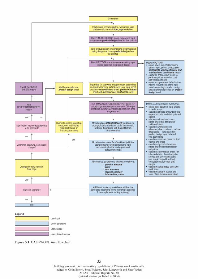
35Building economic decision-making capabilities of Chinese wool textile mills
edited by Colin Brown, Scott Waldron, John Longworth and Zhao YutianACIAR Technical Reports No. 60
(printed version published in 2004)
Figure 5.1 CAEGWOOL user fl owchart
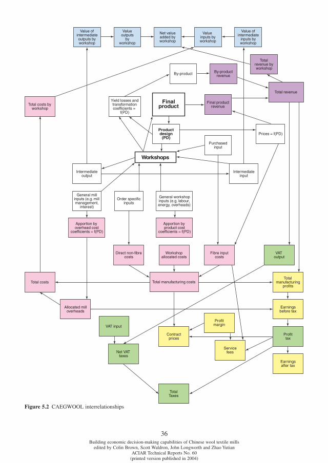
36Building economic decision-making capabilities of Chinese wool textile mills
edited by Colin Brown, Scott Waldron, John Longworth and Zhao YutianACIAR Technical Reports No. 60
(printed version published in 2004)
Figure 5.2 CAEGWOOL interrelationships
37Building economic decision-making capabilities of Chinese wool textile mills
edited by Colin Brown, Scott Waldron, John Longworth and Zhao YutianACIAR Technical Reports No. 60
(printed version published in 2004)
a single profi t tax rate (which is specifi ed as a default value of 33% on the cost input worksheet. However, in practice, the profi t tax rate can vary according to aggregate (as compared with specifi c order) profi ts. Thus, the profi t tax rate specifi ed by the user should be the rate that normally applies to the mill.
The treatment of value added tax is more prob-lematic. There are two separate components to this tax. A value added tax applies to sales (usually at a rate of 17%). However, a rebate (usually at a rate of 13%) can be claimed for inputs. However, this does not apply to all inputs to the manufacturing process. Specifi cally the rebate can be claimed on raw material inputs such as fi bre inputs as well as other manufac-turing inputs. Nevertheless, it cannot be claimed on labour inputs or on mill overheads. The model cal-culates the value added tax on outputs and rebate on inputs in this manner. That is, the rebate is based on the costs of fi bre inputs as well as workshop energy and other costs but excludes labour costs and work-shop and mill overheads. Another complication is that the value added rebate rate can vary according to the specifi c input although the rebate for wool is normally the same rate as for most other inputs. Once again the cost input worksheet allows the user to input the rates for the value added tax on out-puts and the rebate rate for inputs. The model then generates the value added tax amounts for the mill (order) as a whole. Note again that the value added tax is included in mill profi ts prior to the profi t tax described above being applied.
Profi ts, contract prices and service fees
As mentioned, the model is usually based around a product ‘order’ although provision does exist to con-sider multiple orders at the same time. However, the model can present the output either as the profi t from that order, as a contract price or as a service fee.
The profi t statement which appears on the profi t sheet — and is mirrored in items presented on the specifi c workshop sheets — sets out the various revenues, costs and taxes and an after tax net revenue or profi t. Thus, it determines the profi tability of a particular order based on a particular set of product and input prices.
The contract price indicates the product price the mill needs in order to make a specifi ed after tax profi t. Specifi cally, users specify a profi t ‘margin’ which is expressed as a percentage of product costs (including apportioned mill overheads and net value added tax) that users would like to generate as an after-tax profi t for that order. The model then uses this profi t margin, the product or order costs and the tax rates to determine the price needed to achieve this profi t margin. Because the value added tax and the profi t tax depend on the fi nal product price, the
model needs to determine the contract price, profi t tax and value added tax on outputs simultaneously. This is achieved through the equation shown below.
P = C (1 – Tp + M) / (1 – Tp – Tv – Tv M – Tv Tp)Where P = contract price; C = product costs (including
apportioned overheads and value added rebate on inputs); M = profi t margin; Tp = profi t tax; and Tv = value added
tax on outputs.
The service fee covers the case where mills are sup-plied with the raw wool materials and are asked to process them on commission for a service fee. It is calculated in the same manner as the contract price except that it excludes wool input purchase (or direct fi bre) costs.
Intermediate prices and net value added
Many of the outputs from different workshops are not sold but are used as inputs for subsequent processing stages or workshops. Similarly many of the fi bre inputs to different workshops are not purchased but come from workshops involved in a previous stage processing. Thus, in order to determine the true value of particular workshops, an accurate tracking and valuation of these intermediate inputs and outputs must be made.
Intermediate prices are tracked through the model based on input requirements (specifi ed in the product design) and allocated workshop and mill over-head costs. The intermediate price includes all costs incurred through the various stages of the mill to pro-duce the intermediate product including input costs (net of any VAT rebate) and apportioned mill over-head costs. The price excludes any profi t margin and profi t and value added taxes on outputs as mills can elect to produce the intermediate input themselves or alternatively purchase it in from another mill. Both the profi ts and related taxes are based on overall net revenues and so are indifferent as to whether the input cost is a purchased input or the own costs of producing the intermediate product.
There is also some debate when calculating prices for intermediate inputs as to whether mill over-heads should be included. That is, there may be some conjecture that the mill would have incurred the overheads irrespective of whether it produced the intermediate product or purchased it. Thus there may be some debate as to whether the mill over-heads should or should not be included in the inter-mediate price and consideration of opportunity cost. In the intermediate prices sheet, both intermediate prices with and without overhead costs are calcu-lated and compared with market prices to determine the opportunity costs of self-producing inputs. Note that the decision of whether to self- manufacture or purchase-in the intermediate inputs may well change depending on this treatment of mill overhead costs.
38Building economic decision-making capabilities of Chinese wool textile mills
edited by Colin Brown, Scott Waldron, John Longworth and Zhao YutianACIAR Technical Reports No. 60
(printed version published in 2004)
The net revenue or value added by each work-shop is listed in Section C of the profi t sheet as well as in Section 7 of the individual workshop sheets. In these sections, the net revenue added is also broken down into the value of all outputs whether fi nal or intermediate — that is, revenue from fi nal outputs and by-product revenues as well as the value of any inter-mediate outputs (intermediate price times amount) and the value of all inputs whether purchased or inter-mediate — that is, workshop allocated costs, appor-tioned mill overheads, purchased fi bre inputs, and the value of any intermediate inputs (intermediate price times amount). Subtracting the value of inputs from the value of outputs results in the net revenue or value added. Section C of the profi t sheet as well as Section 7 of the individual workshop sheets lists two columns of these values — one inclusive of profi t and value added taxes and rebates and the other exclusive of profi t and value added taxes and rebates.
Apportioning mill overheads
Apart from the fi xed (throughput unrelated) costs that may arise directly in a workshop, there are a number of general mill overheads that are not specifi c to any workshop. These include the costs for the general man-agement of the mill, sales and marketing offi ce, land and other throughput or profi t unrelated taxes, effl uent treatment and other overheads. In order to determine intermediate prices, contract prices and service fees, some apportioning of these overhead costs to partic-ular workshops and products is required. By its nature (in terms of being a fi xed cost), there is no single defi nitive way that overhead costs can be apportioned. The way in which the model apportions these costs is set out below. However, there may be other ways that mill managers consider that these costs should be apportioned and this may require some changes to the relevant part of the Visual Basic code (in the subrou-tine OHEADCOSTS).
In essence the overhead costs are apportioned according to value in a six-step process. In the fi rst step, the mill overheads listed in Section 1 of the cost input sheet are aggregated. In the second step, the value of all mill outputs is calculated by multiplying the workshop throughputs listed in Section 2 of the cost input sheet by the relevant product price (usu-ally the price of the fi rst product specifi ed as being manufactured for that workshop). In the third step, the value of all products manufactured as part of the order is calculated and expressed as a proportion of the total value of mill output calculated in step 2. In the fourth step, the proportions calculated in step 3 are modifi ed according to the (endogenously determined or user specifi ed) product specifi c overhead cost coeffi cients that appear on the overhead cost coeffi cients sheet. That is, these coeffi cients indicate whether a specifi c
product incurs higher overhead costs (relative to its value) than other products. In the fi fth step, the sum of the modifi ed proportions estimated in Step 4 are nor-malised to a value of 1 to ensure that the apportioned mill overheads by product sum to the total mill over-heads for the particular order. Finally, the sixth step applies the modifi ed proportions in step 5.
Part B — Running the Model(Sections 5.3 to 5.7)
This part of the manual provides details on how to complete the various input sheets, how to run the model, how to interpret the output sheets, and how to navigate around the worksheets in the model. As mentioned in Part A, the model is run from a Microsoft Excel spreadsheet. Opening the spread-sheet will take the user to the CAEGWOOL home sheet described in Section 3 below. Note that detailed instructions on how to complete input worksheets or how to interpret output work-sheets also appear at the top of each sheet.
The basic steps in running the model can be summarised as follows:• Step 1 — Open the CAEGWOOL Master
(Microsoft Excel workbook) fi le which will automatically open on to the CAEGWOOL home sheet.
• Step 2 — Use the FRONT PAGE navigation button to go to the front page sheet and enter information as directed on the name of the model run, the workshops to be included, and details of the fi nal outputs.
• Step 3 — Click on the PRODUCT DESIGN macro button, which will send you to the product design sheet and create the input proformas for the fi nal outputs.
• Step 4 — Complete the remaining product design interactively as directed before clicking the CREATE INPUT SHEETS macro button, which will format the remaining input sheets according to the user specifi ed product design.
• Step 5 — Complete the remaining input work-sheets — cost input, prices, product cost coeffi cient, yield coeffi cients, and overhead cost coeffi cients sheets — as directed. Many of the input cells will contain endogenous or default values which can be used by the user or alternatively simply overtyped. (Users can make changes to the way the model calculates some of these endogenous or default values by changing values on the endogenous parame-ters sheet. However, this must be done prior to clicking the CREATE INPUT SHEETS macro button in Step 4.)
39Building economic decision-making capabilities of Chinese wool textile mills
edited by Colin Brown, Scott Waldron, John Longworth and Zhao YutianACIAR Technical Reports No. 60
(printed version published in 2004)
• Step 6 — Once all the input sheets are completed, click on the CREATE OUTPUT SHEETS macro button which is located on the CAEGWOOL home sheet.
• Step 7 — The CREATE OUTPUT SHEETS macro will automatically generate the output sheets, save the fi le according to the model name spec-ifi ed in Step 2, and open the CAEGsummary Microsoft Excel workbook to record the model name and net profi t before and after tax, and to sort the model runs according to ascending order of profi t after tax.
• Step 8 — Exiting the CAEGsummary work-book will return the user to the latest model run, where further model runs can be per-formed as directed by changing input values and clicking on the CREATE OUTPUT SHEETS macro button.
5.3 CAEGWOOL Home page — navigating the CAEGWOOL spreadsheet
The fi rst worksheet that appears in the CAEGWOOL model is the CAEGWOOL home sheet. Apart from some basic information about the model, this sheet is used primarily to navigate around the worksheet and to run some of the key program macros. There are three columns of buttons. The fi rst column con-tains self-titled buttons that hyperlink to all of the input worksheets (e.g. product design sheet). At the bottom of this column is a link to the endogenous parameters sheet accessed for advanced usage of the model. The second column contains buttons that link to the output worksheets common to all model runs (e.g. profi t sheet), and to the workshop-specifi c output worksheets (e.g. spinning sheet). Of course, the sheets in the latter two categories can only be accessed by these macro buttons once they have been generated by the CAEGWOOL model.
Each of the specifi c worksheets (both the input sheets as well as the model generated output sheets) has an arrow labelled with a ‘home’ in their top left hand corner (cell A1). Clicking on this arrow will return the user to the CAEGWOOL home sheet.
The third column contains key program macros. The fi rst of these are the two main program macros, namely CREATE OUTPUT SHEETS (which runs the model and generates the output sheets) and CREATE INPUT SHEETS (which formats the input sheets and inserts model determined values based on the product design). The second set of macro programs, namely DELETE OUTPUT SHEETS, and CLEAR INPUT SHEETS macro programs are used to clear all input
and output sheets in preparation for a completely new product design model run. (A warning is given to highlight that these macro programs will clear all the input.)
5.4 Input sheets
The CAEGWOOL workbook fi le contains a series of seven input worksheets, namely:• front page• product design• cost input• price input• product cost coeffi cients• yield coeffi cients • overhead cost coeffi cients.Instructions to complete the worksheets appear under the title at the top of each one. These instructions are described in more detail below.
The input sheets are completed in sequence and are related. That is, the front page sheet specifi es the product/order being analysed. The product design sheet then specifi es the intermediate inputs needed to produce that product(s). Details entered on the front page and product design sheets are used to automati-cally format the remaining input sheets.
Except where stated, input should be entered in the blue shaded cells.
5.4.1 Front page sheet
The fi rst item to input on the front page sheet (cell C5) is the path name of the fi le to which to save summary results from the model (see Section 7 for more details). The initial default name listed in cell C5 is C:\CAEGsummary.xls. However, as indicated in Section 7, users may want to save these summary results in another location or fi le.
The next item on the front page sheet (cell B8) is the name of the model run. The name specifi ed will be used to create an output fi le of the same name. The name can include a directory path, in which case the fi le will be saved to a specifi c location. Alter-natively, if just a name is given, a fi le of that name will be saved to the default drive for Excel fi les for the user’s computer (see Section 7 for more details). To the right (cell F8), the user is asked to specify whether it is a new design scenario. That is, if there are no output sheets, the user should enter a ‘1’ in this cell, otherwise leave as blank.
Column A of the front page lists various mill workshops or departments. Not all mills have all departments and some products do not use partic-ular departments. The workshops to be considered in the analysis are input into the model by entering a ‘1’ (for yes) in the relevant blue cells in Column B.The workshops not to be included in the analysis
40Building economic decision-making capabilities of Chinese wool textile mills
edited by Colin Brown, Scott Waldron, John Longworth and Zhao YutianACIAR Technical Reports No. 60
(printed version published in 2004)
should be indicated by entering a ‘0’ in the relevant blue cells in Column B, or by leaving blank (being the default for 0).
Columns C and D are then used to enter the fi nal output(s). These are products sold out of the mill and not intermediate products or by-products. Note that fi nal products may be a single fi nal output in the case where a single product/order is being analysed or where they are multiple fi nal outputs. A product label is entered in Column C. The amount is entered in Column D (and the units are specifi ed in Column E. The product label can be any alpha numeric (including Chinese characters, letters or numbers) and so can use any existing mill label for this product. Note that this label will appear on all subsequent input and output sheets.
After completing relevant cells in Columns B, C and D, click on the PRODUCT DESIGN macro button at the top of the page. The PRODUCT DESIGN macro takes you to the product design sheet, clears any existing input on this sheet, and generates the input proforma for the fi nal products specifi ed on the front page sheet. (Thus, re-clicking on the PRODUCT DESIGN macro button will delete all existing product design on the product design sheet.)
5.4.2 Product design sheet
The product design sheet is perhaps the most crucial data sheet. It would be completed by a production or technical manager(s), and sets the precise specifi ca-tions for the raw and intermediate products required to produce the fi nal product. In essence, the product design sheet provides proformas or templates which allow the user to input specifi cations for all fi nal products, intermediate products and inputs.
The product design sheet is completed from left to right. Proformas for fi nal products speci-fi ed on the front page sheet will initially automati-cally appear — following clicking on the ‘PRODUCT DESIGN’ macro button on the front page sheet. (For instance if a fi nished fabric with a product label of ‘fabric601’ is the only fi nal product specifi ed on the front page sheet, then a single proforma will appear in cells A5 to B18, with the product label ‘fabric601’ appearing in cell B6. Conversely, if a yarn was speci-fi ed as a fi nal product, then the proforma would have appeared in cells D6 to E21.) The user completes the proformas for the fi nal product(s), and then clicks on the relevant ‘… DESIGN’ macro button for the next processing stage at the top of the input column. (For instance, if the fi nal product is a fabric, then the user clicks on the ‘YARN DESIGN’ in cell B4.) This will generate proformas for the intermediate and pur-chased inputs specifi ed. The user then completes the proformas, clicks on the ‘… DESIGN’ button and the process repeats.
The fi rst row in the proformas calls for product labels. These labels are used in the design of the subsequent input sheets generated by the model as well as in the output sheets. These labels can be any alphanumeric label including those commonly used by mills.
Note that some items in the proforma are prefi xed with a ‘**’, italicised, and in a coloured font. These items are not used to estimate endogenous para meters in the current version of the model and so are not mandatory to complete. They have been incorporated as they may be useful in subsequent model develop-ment and in describing the product on the output sheets. However, users are not required to enter infor-mation in the blue shaded cells for these items.
Some products specifi ed in the product design will be manufactured within the mill while others may be purchased in from outside the mill. This is indicated in the proforma (in the ‘Manufactured (1) or pur-chased (0)’ row) by specifying a value of ‘1’ in the blue shaded cell if it is manufactured and a value of ‘0’ or left blank if it is purchased. For products specifi ed as being ‘manufactured’, information is required on what inputs are required to produce that product. This information is entered at the bottom of the proforma for each product. The cells ask for how many inputs are required (for example, cell ‘E14’ in the case of the fi rst yarn) and then the input labels and proportions of these inputs that go into making the product. For example, if the fi rst yarn (‘yn1’) required two fi nished tops (‘ftnum2’ and ‘ft1’) made up of 95% of ‘ftnum2’ and 5% of ‘ft2’, then the fi n-ished top labels would be specifi ed in the blue cells D15 to D16 with the proportions specifi ed in cells E15 to E16. These proportions should be entered as percentages rather than decimal fractions and must add up to 100. If they do not, an ‘Error’ message will appear when the ‘… DESIGN’ is pressed for the next processing stage, and the correct proportions adding up to 100 will have to be entered before the model can proceed.
After the proformas for the fi nal product(s) have been completed, the relevant macro button in row 3 should be clicked (for instance, if the fi nal product was a fabric, click on the ‘YARN DESIGN’ macro button in cell B4). Proformas for the intermediate or purchased inputs specifi ed in the fi nal product will then appear. The shaded cells are completed as described above, including specifying inputs and their proportions, and by clicking on the relevant macro button at the top of the column once all the data are entered.
In this way, the user moves from the left to the right of the sheet by completing the empty pro-formas that automatically appear and then clicking on ‘… DESIGN’ at the top of the input columns.
41Building economic decision-making capabilities of Chinese wool textile mills
edited by Colin Brown, Scott Waldron, John Longworth and Zhao YutianACIAR Technical Reports No. 60
(printed version published in 2004)
Note that different products (e.g. different yarns) may use the same input (e.g. a particular fi nished top). For instance, ‘yn1’ and ‘yarn2’ may both use fi nished top ‘ft1’. Thus, when the ‘… DESIGN’ button is clicked, the model checks whether any of the inputs are the same and will only generate the pro-formas once for any particular input — that is, for the example listed above, the model will only gen-erate a proforma for ‘ft1’ once.
Once all product design details have been entered, click on the CREATE INPUT SHEETS macro button in the instructions. This will generate the subsequent input data sheets based on details provided on the product design sheet.
Various numbers will appear in row 4 indicating the number of products at each stage, as the input proformas are generated. These are a normal part of the operation of the model and should not be deleted at any stage.
5.4.3 Cost input sheet
This worksheet is divided into three sections, namely information on mill overheads, workshop costs, and costs specifi c to particular products. These sepa-rate components are discussed below. Note that the CREATE INPUT SHEETS macro run by clicking on the INPUT DATA macro button on the product design sheet will have generated product labels and blue cells for data entry.
Mill (overhead) costs not allocated to workshop (Section 1 — rows 5 to 17)
These include overhead costs that are across the entire mill and not associated with any specifi c work-shop. Examples include general mill management and expenses associated with a sales and marketing team. Note that care should be exercised to exclude any overhead amounts that are included in the work-shop costs (for example, depreciation on capital or workshop manager’s salary in, say, a weaving work-shop. Whether overhead costs are included in the general mill overheads or in the workshop overheads will primarily depend on how these costs are recorded in mill cost records. If information is available on these costs at a workshop level, then they should be included under ‘workshop costs’ rather than under ‘mill overhead costs not allocated to workshop’). As the data on workshop costs and volumes are typical on a monthly basis, the overhead costs should also be specifi ed as a monthly amount.
There are some overhead costs incurred by virtu-ally all mills that are listed in rows 7 to 11, namely: ‘Interest’; ‘Non-profi t taxes’, ‘Depreciation’; ‘Gen-eral Mill Expenses’; and ‘Sales and Marketing’. (Note that while these overheads are incurred by
most mills, it is not mandatory to enter informa-tion on them here.) The monthly amounts for these items should be entered in the blue cells D7 to D11. In addition, the input sheet allows provision for the entry of up to fi ve other types of overhead costs to be included. The names of these other overhead costs should be entered in the shaded cells B12 to B16 with their amounts listed in cells D12 to D16.
In relation to some of the listed overhead cost cat-egories, ‘non-profi t taxes’ should not include value added taxes or profi t taxes as these are automatically calculated within the model (see Section 2.4.1). The non-profi t taxes vary from items such as land tax to welfare taxes, and they can all be aggregated into the one tax. As mentioned above, for items such as ‘interest’ and ‘depreciation’ care should be exercised that these do not include any amounts entered under the workshop costs category mentioned below.
Workshop costs (to be allocated by throughput and coeffi cient) (Section 2 — rows 18 to 29)
This section requires entry of costs of major cost categories for each of the workshops specifi ed on the front page sheet. These categories are based on existing mill data collection and include ‘energy’, ‘wages’, ‘overheads’ (note these are overhead or fi xed costs that are specifi c to the workshop) and ‘other’ (which should be used if costs other than energy, wages and overheads are included). In addition to the cost items, Column D also asks for throughput in the workshop (throughputs are specifi ed in metres for the fi nishing and weaving workshops and in kilo-grams for all other workshops).
Information on costs and throughputs should be on a representative month basis. That is, the costs and throughputs are used to determine a unit cost. The unit cost can then be applied to a product order (depending on volume) and modifi ed according to cost coeffi cients that are entered on the following product cost coeffi cient sheet. Thus a recent ‘normal’ month should be used or alternatively a series of months should be averaged to smooth out any abnormal costs (care should be taken, however, that the averaging does not conceal unit cost variations).
Costs directly attributable to a product order (Section 3 — rows 30 on)
Some costs can be easily identifi ed to a particular order such as certain dyes or specifi c packaging. If this is the case, then these specifi c costs can be entered in this third section of the worksheet. The INPUT DATA macro will generate product numbers, workshops and blue cells. Note that only products that are manu factured by the mill (not bought in) will appear with product labels and blue cells. It is also
42Building economic decision-making capabilities of Chinese wool textile mills
edited by Colin Brown, Scott Waldron, John Longworth and Zhao YutianACIAR Technical Reports No. 60
(printed version published in 2004)
important to note that there may not be any directly attributable costs and so there is no need to enter any data. There is provision for the entry of up to nine separate cost items in each workshop.
If direct costs are entered, then their name should be entered in the relevant blue cells in Column C and the cost (total for product order and not a unit cost) entered in Column D.
Any costs entered in this section should not be included in the costs specifi ed in the previous sec-tion (workshop costs to be allocated by throughput and coeffi cient). For instance, in specifying any direct dye or packaging costs, care should be exer-cised in ensuring that these dye and packaging costs are not included in the workshop costs to be allo-cated. In general, if the information is available, it is preferable to enter costs directly in this section rather than in the workshop allocated costs section because the latter will be allocated by general cost coeffi cients only.
5.4.4 Price input sheet
This sheet requires input of prices of products (fi nal, intermediate and purchased input prices) as well as the prices of the various by-products produced along with margins and tax rates. The sheet is organised into four sections based on these categories.
In Section 1 (‘Product prices’), prices for all prod-ucts (fi nal and intermediate) are entered. Based on the front page and product design sheets, the INPUT DATA macro will automatically enter the product labels for products requiring price data to be entered. This macro will also list the endogenously deter-mined prices in the shaded cells below the product labels. These prices are a guide, however, and the user may enter their own prices simply by typing over the amounts in the shaded cells. The determina-tion of endogenous prices is described separately in Section 5.9.2. Thus, the sheet is designed to provide information (and specifi c model values) on prices for particular products, but also allow the user to easily overwrite these endogeneously determined prices if they have more specifi c knowledge. In addition, managers interested in knowing the impact of vari-able prices can run alternative scenarios with partic-ular prices.
In Section 2 (‘by-product prices’), various by-products and endogenously determined prices appear in cells A28 to B35. Once again, the user can simply overtype the values in the shaded cells if they want to generate scenarios based on a different set of prices.
In Section 3 (‘Margin’), the shaded cell (cell B38) is where the user enters a profi t margin. The margin represents the percentage mark up over all costs (including taxes) that the mill/user would like to receive or needs to recover. The margin is used
in the model to estimate service fees and contract (sales) prices.
In Section 4 (‘Tax’), tax rates that are used to endogenously calculate three specifi c tax items in the model are specifi ed. The fi rst relates to the profi t tax rate, the second to the value added tax rate on outputs, and the third to the value added rebate on inputs. Note that all of these rates are specifi ed in percentage terms (e.g. profi t tax of 33). Default rates (based on the actual values in 2004) are set in the shaded cells. However, because these rates can and do change, users can overwrite these values.
5.4.5 Product cost coeffi cients sheet
The Product cost coeffi cients sheet is used to enter information on cost coeffi cients to be used in the allocation of workshop costs. That is, workshop costs may be allocated to products initially based on volumes (that is, unit costs). However, some prod-ucts may be more expensive to produce in partic-ular workshops (use more labour or energy, etc) than other products. Thus cost coeffi cients can be used to more accurately assign workshop costs to a partic-ular product. The cost coeffi cients are an integral part of the model and of the ACIAR project and are dis-cussed in detail in Chapter 2.
The cost coeffi cients should be specifi ed on the basis that the most common product has a cost coef-fi cient of 1 or that costs are allocated to products on the basis of throughput alone. The specifi c coeffi -cients for specifi c products should then be expressed relative to this normal, common or standard product. For instance, a cost coeffi cient of 1.1 indicates that the unit cost of a particular product is 110% of the unit cost based on throughput alone or of the unit cost for a standard product.
The sheet lists all possible workshops down the page with major cost categories listed (in Column B) for each workshop. (That is, product cost coeffi cients should be specifi ed not only by product but also by cost category.) However, the INPUT DATA macro button ensures that only the workshops and prod-ucts indicated on the front page and product design sheet will appear on the product numbers and as blue shaded cells. As the model requires some input for these coeffi cients, the shaded cells automatically have a value of 1 (that is, unit costs based on share of throughput alone) or some other endogenously deter-mined cost coeffi cient based on the product design as described in Chapter 2. Users can type new values over these default or endogenously determined values if they have more specifi c knowledge of these cost coeffi cients. Users may also want to investigate var-ious scenarios (such as technology reducing the costs of producing a particular type of product).
43Building economic decision-making capabilities of Chinese wool textile mills
edited by Colin Brown, Scott Waldron, John Longworth and Zhao YutianACIAR Technical Reports No. 60
(printed version published in 2004)
5.4.6 Yield coeffi cients sheet
Products are transformed at each stage of the wool textile processing chain. In some cases this involves distinct changes in units (for example from kilograms of yarn to metres of fabric), while yield losses are also associated with the processing. These by- or co-products, such as noil, spinning wastes, etc., can be sold albeit at a lower price than the original product. Thus the model needs to keep track of the physical amounts of each product at the different stages and to do so needs accurate yield coeffi cients. A spinning yield coeffi cient of 0.95, for instance, indicates that only 95% of the weight of fi nished tops entering the spinning stage is refl ected in the weight of the yarn produced. Yield coeffi cients are assumed to depend not only on output characteristics but also on input characteristics of the product. This is the format refl ected in the sheet. Further details about the deter-mination of these yield coeffi cients are provided in Section 5.9.4.
Initially this sheet will simply have the heading ‘Yield coeffi cients’. However, the INPUTSHEETS macro will generate the products considered in the analysis based on the information on the front page sheet and product design sheet. Blue shaded cells will again guide input. As the model requires some input for these coeffi cients, the blue cells will auto-matically have a value of 1 (that is, no yield losses) or some other endogenously determined or speci-fi ed coeffi cient. Users may input their own yield losses by overtyping these values with their own specifi c estimates of the yield coeffi cients. As men-tioned, the characteristics of both inputs and out-puts can infl uence yield coeffi cients and so there is a matrix of yield coeffi cients specifi ed on the sheet for each workshop/stage, with the output products listed on the columns and the input products speci-fi ed in the rows. If yield coeffi cients are assumed to vary only according to the output type, then this can be achieved simply by listing the same values in an output product column.
Note that the yield coeffi cients are expressed as a decimal fraction rather than as a percentage. Thus, a yield coeffi cient of 0.93 would have a recombing loss of 7%.
5.4.7 Overhead cost coeffi cients sheet
The Overhead cost coeffi cients sheet is used to enter information on cost coeffi cients to be used in the allocation of mill overhead costs. Because of the nature of overhead costs, they will normally be allo-cated to products based on volumes alone (that is, unit costs). However, some products may draw more heavily on overhead cost categories (for instance, require more managerial or sales and marketing
input) than other products. Thus, overhead cost coef-fi cients can be used to more accurately assign these general mill costs to a particular product. The coef-fi cients are specifi ed in the same way as the product cost coeffi cients. For instance, an overhead cost coef-fi cient of 1.1 indicates that the unit overhead cost of a particular product is 110% of the unit cost based on throughput alone. Note that because of their nature and diffi culty in determining any variation across products, most model runs may well have over-head cost coeffi cients all specifi ed as ‘1’. However, as a general model, it is important to allow for other co effi cients or other allocations of overhead costs if specifi c information is available. These issues and other details about the overhead cost coeffi cients are discussed in Section 5.9.5.
The sheet lists all possible workshops down the page. However, the INPUT DATA macro ensures that only the workshops and products indicated on the front page and product design sheet will appear on the product numbers and as blue shaded cells. As the model requires some input for these coeffi cients, the shaded cells automatically have a value of 1 (that is, unit overhead costs based on share of throughput alone) or some other endogenously determined cost coeffi cient based on the product design. Users can type new values over these default or endogenously determined values if they have more specifi c knowl-edge of these cost coeffi cients or if they want to investigate various scenarios (such as technology reducing the costs of producing a particular type of product).
Once the Overhead cost coeffi cient sheet has been completed (and all the others) the model is ready to run and generate output. This can be achieved by returning to the CAEGWOOL home sheet and clicking on the CREATE OUTPUT SHEETS macro button.
5.4.8 Re-entering input data
After the model has been run, data can be re-entered and new scenarios/model runs conducted as high-lighted in the fl owchart in Figure 5.1. Three types of new scenarios can be considered. First, the impact of slight changes in input data (prices, cost coeffi -cients, etc.) or where different amounts of the fi nal product (of the same design) are of interest. In this case, modify the relevant coeffi cients, return to the front page sheet and enter a new model run name, before clicking the CREATE OUTPUT SHEETS macro button on the CAEGWOOL home sheet which will automatically delete the old output sheets and gen-erate the new output sheets. Note that in this case, the shaded cell for ‘new design scenario’ should be blank or ‘0’ to indicate that output sheets already exist.
44Building economic decision-making capabilities of Chinese wool textile mills
edited by Colin Brown, Scott Waldron, John Longworth and Zhao YutianACIAR Technical Reports No. 60
(printed version published in 2004)
Second, scenarios may involve essentially the same fi nal product order but with slightly different product design requiring a few new (intermediate input) products to be specifi ed on the product design sheet. In this case, the new product design can be entered by clicking on the relevant reset (R) and … DESIGN macro buttons and completing the new product pro-formas. The INPUT SHEETS macro can then be re-run, with any additional data entered on the price, cost coeffi cient and yield coeffi cients sheets.
Third, more fundamentally different scenarios — such as entirely new fi nal products or completely dif-ferent product design specifi cations — require a new set of input sheets. In this case, click on the DELETE OUTPUT SHEETS macro button as well as the CLEAR INPUT SHEETS macro button on the CAEGWOOL home sheet.
Note that the output from new model runs is stored in a separate Excel fi le depending on the name speci-fi ed in cell B8 of the front page worksheet. Thus, it is important to specify a new model run name.
5.5 Common output work sheets
Once the create output sheets macro button has been clicked, a set of output sheets are automatically gen-erated. These include a set of fi ve output sheets that are common to all model runs namely:• Physical amounts sheet• Profi t sheet• Cost details sheet• Revenue details sheet• Intermediate prices sheet.In addition, detailed workshop sheets are gener-ated for each workshop included in the analysis. In Section 5, the common output sheets are described, while Section 6 describes the workshop specifi c output sheets.
Note that the output work sheets precede the input work sheets in the saved model Excel workbooks. They can also be accessed via the navigation buttons on the CAEGWOOL home sheet
5.5.1 Physical amounts sheet
The physical amounts sheet lists all the physical fl ows of product through the mill based on the fi nal outputs specifi ed and the design of the product. It is divided into two sections — the fi rst section out-lines the physical fl ow of the products specifi ed on the front page sheet or product design sheet, while the second section lists the amounts of co- or by- products produced in each of the workshops as part of the processing.
Specifi cally, Section 1 (‘products’) reports the amount of each product specifi ed on the product design sheet (indicated by the product label in
Column B) and sorts it into the category of fi nal output (Column C), intermediate input (Column D) or purchased input (Column E). Note that in the input sheets, only the amount of fi nal product is specifi ed. The amount of the other intermediate inputs and pur-chased inputs is calculated in the model from the fi nal product amount, the product design specifi ca-tions (products required and proportion), and the yield coeffi cients.
In Section 2 (‘by-products’), the amounts of by-products produced are reported. Once again these are derived through the product design specifi cations, yield coeffi cients and fi nal product amount.
The physical amounts sheet will be of interest to a number of managers within the mill. Workshop pro-duction managers will have direct information on how much product they need to produce (as inter-mediate input) to meet the fi nal order. Similarly mill buyers will know what types and amounts of prod-ucts they need to purchase for each workshop.
5.5.2 Profi t sheet
The profi t sheet contains three separate components, namely: (A) Profi t statement; (B) Contract prices and service fees; and (C) Net revenue added by workshop.
Section A. ‘Profi t statement’ sets out a profi t state-ment or statement of costs, revenues and net revenues. These are based on the format of profi t statements that mills/Chinese enterprises are familiar with. Item ‘1’ (row 6) is ‘total revenue’ which is disaggregated in the following two rows into ‘fi nal output’ reve-nues and ‘by-product’ revenues. Item ‘2’ (row 10) specifi es ‘total manufacturing costs’ and reports the total of the costs incurred in the workshops. These are also disaggregated into three categories, namely costs allocated by (product cost) coeffi cients, direct costs attributable to products (such as a specifi c dye or packaging but not fi bre inputs), and direct fi bre input costs.
Subtraction of the total manufacturing costs from the total revenue gives Item ‘3’ (row 15) of ‘manu-facturing profi t’. Item (‘4’ — row 17) reports ‘mill overhead costs’ which are then disaggregated into ‘interest’, ‘value added taxes’, ‘taxes other than profi t or value added’, ‘depreciation’, ‘general mill expenses’, ‘sales and marketing’ and ‘other mill over-heads’. These are based on the values entered in the Cost input sheet as well as the overhead cost coeffi -cients and tax rates. Note that in line with Chinese accounting practices, mill overheads include interest, value-added taxes and non-profi t taxes but exclude profi t tax.
The mill overhead costs (Item ‘4’) are then sub-tracted from the manufacturing profi t in Item ‘3’ to arrive at Item ‘5’ of Profi t before tax (row 26). Item
45Building economic decision-making capabilities of Chinese wool textile mills
edited by Colin Brown, Scott Waldron, John Longworth and Zhao YutianACIAR Technical Reports No. 60
(printed version published in 2004)
‘6’ is a ‘profi t tax’ which is calculated by multiplying the profi t tax rate by the profi t before tax (Item ‘5’). Subtraction of the profi t tax (Item ‘6’) from the profi t before tax (Item ‘5’) results in Item ‘7’ of ‘profi t after tax’.
Section B. ‘Contract prices and service fees’ reports contract prices and service fees for the fi nal products specifi ed.
The contract price is calculated as total product costs including taxes plus a profi t margin — which is specifi ed on the prices sheet — divided by the amount of the fi nal product (order). Further details about how this price was calculated are set out in Section 5.9.2. As indicated in Section 5.2.4, because profi t tax and value added tax depend on the output price, both these taxes and the contract price need to be determined simultaneously. The contract price indicates the price the mill needs in order to make a specifi ed after tax profi t.
The service fee is the same as the contract price except that it excludes wool input purchase (or direct fi bre) costs. That is, it covers the case where mills are supplied with the raw wool materials and are asked to process them on commission for a service fee.
Section C. ‘Net revenue added by workshop’ reports the net revenue added by each workshop as described in Section 5.2.4. Note that these fi gures include pro-vision for the valuation of both intermediate out-puts and inputs. Column E reports these net revenues added excluding value added and profi t taxes while Column F reports these net revenues added including value added and profi t taxes. As the revenue added at each workshop stage includes provision for profi t margins and taxes in Column F, summing the net revenue added of all the workshops in this column should equate (after rounding errors) with the Profi t after tax reported as Item ‘7’ in Section A. (Note that the sum of net revenues added in Column E (that is, excluding value added and profi t taxes) should equal Item ‘5’ minus the value added taxes reported in Item ‘4’.) Further details of how these net revenues added by the workshops are calculated, are provided in Section 5.2.4.
5.5.3 Cost details sheet
This sheet provides a complete breakdown of costs, the aggregate amounts of which were listed on the profi t sheet. It comprises fi ve separate sections.
Section 1. ‘Workshop allocated costs’ reports the allocated workshop costs by workshop and by the cost categories of energy, labour, workshop overheads and other workshop costs. The costs are also aggregated across workshops and across the cost categories.
Section 2. ‘Workshop direct costs — non-fi bre’ reports the direct costs by workshop for the fi nal outputs specifi ed. While these costs come directly from the Cost input sheet, their presentation in this sheet allows them to be compared with the other cost types. In this section, Column B indicates the type of product (e.g. yarn), Column C the product label, Column D the type of the direct cost, and Column E the cost — which is the cost per order and not a per-unit cost.
Section 3. ‘Workshop direct costs — fi bre’ lists the fi bre input costs for each workshop. The workshops (e.g. weaving) are highlighted in bold in Column B, and this fi rst row lists the total for the workshop. Sub-sequent rows list the type of fi bre input in Column B (e.g. yarn), the product name of the fi bre input in Column C and the cost in Column D.
Section 4. ‘Mill overhead costs’ apportions mill overhead costs for the product order(s) to partic-ular workshops and even specifi c products (fi nal and intermediate products). The columns are the same as for Section 3.
Section 5. ‘Taxes’ lists details of the key taxes. First, it disaggregates value added taxes into its two com-ponents, namely the value added tax on outputs and the value added rebate on inputs. The value added rebate on inputs is actually a revenue. Subtracting this from the value added tax on outputs gives the value listed under ‘value-added taxes’ in Item 4 of the profi t sheet. The following row reports the profi t tax (Item 6 of the profi t sheet), and the next row lists taxes other than for profi t and value added (that also appears as a separate line in Item 4 of the profi t sheet).
This worksheet will be of particular interest to mill accountants and managers in being able to better apportion mill costs to particular workshops and so better understand the cost implications of particular product orders.
5.5.4 Revenue details sheet
The revenue details sheet is a straightforward sheet divided into two sections. The fi rst section — ‘1’ (‘Value of fi nal outputs’) — indicates the reve-nues from the fi nal outputs sold. The type of output is listed in Column B, the product name in Column C, and the revenue in Column D. The second section — ‘2’ (‘By-product revenues’) — indicates the revenues from various by-products. These revenues are derived from the physical amounts (calculated within the model and reported on the physical amount sheet) and the prices (listed on the prices sheet).
46Building economic decision-making capabilities of Chinese wool textile mills
edited by Colin Brown, Scott Waldron, John Longworth and Zhao YutianACIAR Technical Reports No. 60
(printed version published in 2004)
5.5.5 Intermediate prices sheet
The intermediate prices sheet highlights the prices and values of all of the intermediate inputs specifi ed on the product design sheet and whose physical amounts are listed in Column D of the physical amounts sheet. The columns in the sheet are as follows:• Column A lists the type of intermediate input
(e.g. raw top).• Column B indicates the product label of the
intermediate input.• Column C lists the calculated intermediate price.
This intermediate price includes all costs incurred through the various stages of the mill to produce the intermediate product. These include input costs (net of any VAT rebate) and apportioned mill overhead costs, but exclude the profi t margin and taxes. More details of how these intermediate values are calculated are provided in Section 5.2.4.
• Column D lists the market price of the intermediate input (that has either been entered exogenously on the prices sheet or determined endogenously in the model) net of any value added rebate.
• Subtracting Column D from Column C highlights the opportunity cost. That is, if the intermediate price exceeds the market price then there is an opportunity cost for the mill to produce the intermediate input themselves. Intermediate inputs, for which there is a positive opportunity cost(i.e. better to purchase the intermediate input rather than produce it themselves), are highlighted by gold shading. Intermediate inputs which have a negative opportunity cost (i.e. better for the mill to produce itself rather than purchase) are highlighted in green shading.
• Column F lists an intermediate price for the intermediate inputs that does not include mill overhead costs. Column G indicates the opportunity cost when mill overhead costs are excluded (see Section 5.2.4 for a discussion surrounding the issue of whether to incorporate overhead costs). Note that the decision of whether to self-manufacture or purchase in the intermediate inputs may well change depending on this treatment of mill overhead costs.
• Column H lists the contract price and Column I the service fee for the intermediate inputs. These items are calculated in the same way as they were for the fi nal products on the profi t sheet as outlined in Section 5.2.4, namely total costs (intermediate price) plus provision for profi t margin, profi t tax and value added tax on outputs. As discussed in Section 5.2.4 (B), the service fee excludes purchased fi bre inputs. The contract prices for the intermediate inputs enable the mill to ascertain the price it would need to charge before considering selling out some of the intermediate inputs it produces.
Care needs to be exercised in interpreting this sheet. The row shadings should not be the only basis about which intermediate products should be self- manufactured or instead purchased in. An important factor is that conjecture exists about the treatment of mill overheads and non-profi t taxes.
5.6 Run-specifi c (workshop) output sheets
Apart from the output sheets mentioned in Section 5.5 that are common to all model runs, a number of work-shop output sheets (sorting, scouring, topmaking, recombing, spinning, weaving, fi nishing) will also be generated, depending on the workshops included in the analysis. The basic format of all of these sheets is the same and the various sections are described below. However, some sheets do vary slightly and may not include particular sections. For instance, the fi nishing sheet will not include the section on ‘3. Fibre input price/costs’ as the model assumes that all ecru fabric that comes into the fi nishing workshop is not purchased in, but instead is produced in, the mill’s weaving workshop. Similarly, most workshop sheets will not include the section on ‘5. Revenues’ as they will be producing intermediate outputs rather than fi nal outputs.
The fi rst section of a workshop sheet — Section 1. ‘Specifi cations&amounts’ — sets out again the spec-ifi cation of each product at this workshop stage (for example, yarn in the spinning workshop) according to information from the product design sheet. The specifi cations for each product are set out in sepa-rate columns from Column D. For most of the work-shop sheets, whether the product is purchased in or manufactured in the workshop is listed at the bottom of the product specifi cation. If the product is pur-chased in, there are no workshop costs for that par-ticular product. This will be apparent as there will be no cost entries in the rows below this product. The amount required of the product (whether purchased in or manufactured in the workshop) is also indicated at the bottom of this section.
The second section of a workshop sheet — Section 2. ‘Input/output table’ — indicates the amount of inputs required to produce each of the products that are manufactured in the work-shop. (Products not manufactured in the workshop but purchased in as inputs for subsequent stages appear in the product specifi cations but do not fea-ture in this input/output section.) The row under the column headings for this section lists the labels for the products produced in the workshop. The labels of the inputs are then listed in subsequent rows in Column D. This gives three sets of columns for each product manufactured in the workshop. The fi rst set of columns specifi es the proportion of each input
47Building economic decision-making capabilities of Chinese wool textile mills
edited by Colin Brown, Scott Waldron, John Longworth and Zhao YutianACIAR Technical Reports No. 60
(printed version published in 2004)
used to produce the workshop product. The second set of columns highlights the yield coeffi cients. The third set of columns indicates the amount of inputs required to produce each of the manufactured work-shop products. This amount is based on the input proportions, the yield coeffi cients and the amount of workshop product required which is listed in the above Section 1 (‘1. Specifi cations&amounts’). Note that different products manufactured in the workshop may use the same fi bre input. Thus, the fi nal column indicates the total amount of each input required to manufacture all of the workshop products needed, and so provides a guide to the workshop production manager about what fi bre inputs he needs to source.
The third section of a workshop sheet — Section ‘3. Fibre input prices/costs’ — sets out the purchase cost for each of the inputs purchased which is calculated from the physical amount in the input/output table and the price of the input which comes from the prices sheet. This price is also reported in this section in the right-hand column. Note that some workshops that do not purchase in inputs (that is, uses intermediate inputs from other workshops) will not have this section on their workshop sheet.
The fourth section of a workshop sheet is Section ‘4. … workshop costs’. Each product man-ufactured in the workshop has a series of cost cat-egories listed in separate columns from Column E. These are: workshop allocated costs by type; work-shop direct costs — non fi bre; workshop direct costs — fi bre costs; and fi nally total workshop costs with and without allocated mill overheads.
The fi fth section of a workshop sheet — Section ‘5. Revenues’ — lists the price, amount and revenues from the fi nal outputs from the workshop. Because most workshops will not have fi nal outputs, then this section will not appear in most workshop sheets.
The sixth section of a workshop sheet — Section ‘6. Total … workshop costs and revenues’ — lists the aggregate revenue and cost categories for the entire workshop, rather than for individual products.
The seventh section of a workshop sheet is Section ‘7. Value added for … ’. It has three rows and two columns. The three rows are for the: value of all inputs to the workshop (purchased or other-wise); value of all outputs from the workshop (sold or otherwise); and the value added (the value of outputs minus the value of inputs. More details about how these values are calculated are set out in Section 5.2.4. The fi rst column (Column E) lists these values excluding value added and profi t taxes, while the second column (Column G) lists these values including value added and profi t taxes. The values for value added correspond with the items shown in Section C of the profi t sheet.
5.7 CAEGsummary fi le and saving model results
For any particular model run or scenario, the SAVERESULTS subroutine macro saves the gener-ated output sheets along with the input sheets in a fi le with the name specifi ed in cell B8 on the front page worksheet. Note that this fi le will be located in the default Excel drive location on the user’s computer. (Users can change this default location at any time in Excel through <<tools>>, <<options>>, <<general>>and specifying a new location in the default fi le location box.) Alternatively, the name in cell B8 may also include a specifi c path (e.g. C:\\mill runs\scenario1). The latter option may provide a more secure basis for identifying the exact location of the saved fi le. The net profi t from this scenario along with the name of this model run is then recorded in a separateExcel fi le which is initially named by default asc:\CAEGsummary.xls.
When a new model scenario is run, the SAVERESULTS subroutine macro automatically enters the name of the model run in Column A, the net profi t before tax in Column B, and the net profi t after tax in Column C from the new model run into the CAEGsummary fi le. It then sorts the models into descending order of net profi t after tax (namely based on the values in Column C). The latest model run is highlighted by shaded (coloured) cells to indicate how it compares with previous model runs. Appendix Figure 5.18 shows the output from an example CAEGsummary fi le indicating these features. Thus, the user is able to quickly identify how the model scenario compares with other scenarios and the ‘optimal’ scenario (in terms of net profi ts). The fi le containing the output and input sheets for this optimal model run can then be easily identifi ed by the model name.
This fi le will be especially useful when consid-ering alternative fi bre input choices to produce a par-ticular output. The user may delete any of the rows (that is, different model runs) without consequence. This is useful if the user wants to compare an entirely different set or group of model scenarios. There is no need to remove the coloured shading if these rows are complete as the SAVERESULTS subroutine macro will automatically do this before entering the results for a new model run.
Note that provision exists in cell C5 on the front page worksheet to change the path and name of the summary results fi le from the defaultc:\CAEGsummary.xls to another path and fi lename (both the path and fi lename must be specifi ed). In this way, users can maintain several summary fi les which record the results of closely related model runs. It enables the user to direct the fi le to a specifi c path or location allowing it to be easily found at a later stage.
48Building economic decision-making capabilities of Chinese wool textile mills
edited by Colin Brown, Scott Waldron, John Longworth and Zhao YutianACIAR Technical Reports No. 60
(printed version published in 2004)
Each saved fi le can exceed 1 megabyte in size. Thus, if a large number of runs are performed and there is limited storage capacity on the system, the size of the fi les may become an issue. One way to markedly reduce the size of the fi les is to save and run fi les without the macros. This can be achieved by copying all worksheets to a new workbook which will effectively save the fi le without the macros. To run a new model run from the (non-macro) fi le, click on the macro buttons which will simply use the macros of the same name in the other fi le. The saved fi le, as with the original fi le, will be the smaller fi le containing no macros. In this way, numerous model runs can be performed with saved fi les of a much smaller size.
Part C — Advanced Usage(Sections 5.8 and 5.9)
This part of the manual provides details on how to access the Visual Basic code and how to change some of the endogenous parameters in the model both at run time and in model develop-ment. Normal model users will not need to access this section other than as (advanced) specifi ca-tion information on the model. However, it does describe the endogenous parameters sheet which allows users to change endogenous model param-eters without recourse to the Visual Basic code.
5.8 Visual Basic programs
The Excel spreadsheet is used primarily as an input and output platform with all of the computations undertaken in Visual Basic programs as program macros. The macro programs can be accessed and reviewed by clicking on ‘tools’ and then ‘macros’ on the Excel main menu bar. In addition to the macro programs, there are also various subroutine programs called by these macros. The macro programs can be classifi ed into various groups which are described below.
5.8.1 Main program macros
The two most important macros in the program are the MAIN macro and the INPUTSHEET macro as described below:• MAIN: The main program uses information from
the input sheets to calculate all of the costs, revenues and physical amounts. It contains a series of subroutines — one for each output sheet — to generate the output. Note that it also deletes the existing output sheets prior to a new model
run being generated, which is necessary to avoid Microsoft Excel errors being generated in having output sheets of the same name. (Note that the Windows/Excel warning message ‘Delete output sheet permanently’ will appear on a number of occasions as the sheets are being deleted, and just require that OK be clicked.) This macro can be run by clicking a macro button with the label of ‘CREATE OUTPUT SHEETS’ on either the CAEGWOOL home, front page, or overhead cost coeffi cients sheets. Once the output sheets have been created, the value in cell F8 on the product design sheet is made blank to signify that it is not a new scenario (this avoids any errors for the next time the ‘CREATE OUTPUT SHEETS’ button is pressed.
• INPUTSHEET: Used to construct/format workshop costs, prices, cost coeffi cient, and yield coeffi cient sheets from the information contained on the front page and product design sheets. The main purpose is to simplify the input sheets to the maximum extent possible and to minimise misunderstanding and transcription errors by, for example, including only products from the product design sheet and highlighting their labels. This macro can be run by clicking a macro button with the label of ‘CREATE INPUT SHEETS’ on the product design sheet.
5.8.2 Calculation subroutine programs called by main macro
The main macro program calls various subroutine programs to perform a variety of calculations. These subroutine programs can be accessed at the end of the main macro program. These include:• OHEADCOST — reads in overhead costs and
allocates overhead costs to products and workshops
• ENTERFINALOUTPUTAMOUNTS — reads in final outputs as specifi ed on front page sheet
• ENTERPRICEDDATA — reads in information from prices sheet
• ENTERYIELDCOEFFICIENT — reads in yield co-effi cients from yield coeffi cient sheet
• ENTERCOSTCOEFFICIENT — reads in cost co-effi cients from cost coeffi cient sheet
• MODIFYVALUEADD — modifies value of outputs and value of inputs at each stage to allow for value added tax and profi t tax
• PHYSICALC — calculates inputs required and intermediate outputs produced based on fi nal outputs, product design and yield coeffi cients
• ENTERFINALOUTPUTAMOUNTS — reads in final outputs as specifi ed on front page sheet.
49Building economic decision-making capabilities of Chinese wool textile mills
edited by Colin Brown, Scott Waldron, John Longworth and Zhao YutianACIAR Technical Reports No. 60
(printed version published in 2004)
5.8.3 Output worksheet subroutines called by main macro program
After entering input data and calculating physical amounts, the main macro program calls various sub-routine programs that generate the output worksheets. Specifi cally the following subroutine macros (located at the end of the main macro program) generate the worksheets of the same name:• PHYSICAL• PROFIT• COSTDETAILS• REVENUEDETAILS• INTERMEDIATE PRICE• FINISHING• WEAVING• SPINNING• RECOMBING• TOPMAKING• SCOURING• SORTING.
5.8.4 Macros and subroutine macro programs used to save model results and prepare worksheets for new model run
The SAVERESULTS subroutine macro that is called from the MAIN macro saves the model as a Microsoft Excel workbook with user specifi ed name on the front page sheet. The subroutine also records the model name together with the net profi t before tax and the net profi t after tax on the CAEGsummary workbook which records all model runs, and high-lights and sorts the new model run (according to net profi t after tax) on this workbook.
The following two macros are important in pre-paring the model for a new model run and for clearing input sheets to enter a new product design.• DELETEOUTPUTSHEETS: This macro deletes
existing output sheets prior to a new model run (necessary to avoid errors being generated in the MAIN macro which generates output sheets of the same name). Normally the macro is called as a subroutine from the MAIN macro program. However, the macro can also be run independently by clicking on the ‘CREATE OUTPUT SHEETS’ on the CAEGWOOL home sheet of the MAIN macro to delete existing output sheets. When the macro is run from the ‘DELETE OUTPUT SHEETS’ button on the CAEGWOOL home sheet, it sets the value in cell F8 on the product design sheet to ‘1’ to signify that there are no output sheets and that the model is now set up to run a new scenario. ‘Delete output sheet permanently’ will appear on a number of occasions as the sheets are being deleted, and just require that OK be clicked.
• CLEARINPUTSHEETS: Used to clear particular cells on input sheets in preparation for a new product design.
5.8.5 Macros associated with product design sheet
There are a series of macro programs designed to determine what products need to be specifi ed on the product design sheet. A series of subroutines then create the blank proformas for these products on the product design sheet. These macros include:• PRODUCTDESIGN: Clears the product design
sheet and then calls on the program macros below to create the blank proformas for the fi nal outputs recorded on front page sheet.
• PDYARN: Determines what yarn input proformas are required and calls on YARNPD macro to create these proformas.
• PDFTOP: Determines what fi nished top input proformas are required and calls on FTOPD macro to create these proformas.
• PDRTOP: Determines what raw top input proformas are required and calls on RTOPD macro to create these proformas.
• PDSWOOL: Determines what scoured wool input proformas are required and calls on SWOOLD macro to create these proformas.
• PDGWOOL: Determines what greasy wool input proformas are required and calls on GWOOLD macro to create these proformas.
• PDGWOOL: Determines what greasy wool input proformas are required and calls on GWOOLD macro to create these proformas.
The macro programs above call specifi c subroutines described below that create the product proformas. The subroutines can be accessed via the relevant macro program (e.g. access YARND through the PDYARN macro program).• FABRICDESIGN: Creates a blank proforma/form in
Columns A and B of the product design sheet for inputting data on a specifi c fabric.
• YARND: Creates a blank proforma/form in Columns D and E of the product design sheet for inputting data on a specifi c yarn.
• FTOPD: Creates a blank proforma/form in Columns G and H of the product design sheet for inputting data on a fi nished top.
• RTOPD: Creates a blank proforma/form in Columns J and K of the product design sheet for inputting data on a specifi c raw top.
• SWOOLD: Creates a blank proforma/form in Columns M and N of the product design sheet for inputting data on a specifi c scoured wool.
• GWOOLD: Creates a blank proforma/form in Columns D and E of the product design sheet for inputting data on a specifi c yarn.
50Building economic decision-making capabilities of Chinese wool textile mills
edited by Colin Brown, Scott Waldron, John Longworth and Zhao YutianACIAR Technical Reports No. 60
(printed version published in 2004)
Apart from these macros, there are a series of other macros called FABRICDESIGNRESET, YARNDESIGNRESET, FINISHEDTOPDESIGNRESET, RAWTOPESIGNRESET, SCOUREDWOOLDESIGNRESET and GREASYWOOLDESIGNRESET, which are designed to clear or reset the product input proformas on the product design sheet if an error is made and the user wants to input a completely new design. These reset macros can be run by clicking on the ‘R’ macro button at the top of the relevant column on the product design sheet.
The macros use a large number of variables many of which are common to all macros. Note, however, that a full description of all the variables appears at the start of the MAIN macro where all variables are used.
5.9 Endogenous input values and endogenous parameters sheet
There are several areas in the model where the values for particular inputs are calculated endogenously. That is, automatic values will appear on the input sheets based on calculations performed within the model and according to specifi cations/attributes of the product entered on the product design sheet. These values are not intended to be defi nitive but rather to provide a useful guide for users of the model as they are entering various input parameters. Indeed, they are based on empirical sector wide analysis and so cannot be expected to relate directly to any one par-ticular mill.
The main inputs for which endogenous values are calculated or could be considered for calculation are: prices; product cost coeffi cients; yield coeffi -cients; and overhead cost coeffi cients. The estimation of some of these endogenous values has been based on detailed empirical analysis, which is reported in Chapters 2 to 4. This section outlines how and where the fi ndings from these empirical analyses are included in the model and how they can be modifi ed by the user to account for mill specifi c analyses.
In essence, the endogenous values are calculated within the INPUT SHEETS macro. The endogenous values are based on product attributes specifi ed on the product design sheet. These values may be estimated by structural equations with the product attributes as independent variables, or alternatively the product attributes may sort the product into a particular group or type which has a particular (endogenous) value associated with it.
The Visual Basic code highlights where these values are calculated within the input sheets macro by delineating the sections with asterisks (*****) and through relevant comment lines. The variables in the structural equations or that relate to particular product groups are linked to values on the endogenous
parameters sheet. This sheet — described below — lists key values which the user has the opportunity to enter or modify. Thus, the user has easy access to refi ning or tailoring the parameters to their specifi c case if they have the relevant information. However, more fundamental changes — such as different func-tional forms — may require that the relevant Visual Basic code in the highlighted sections of the INPUT SHEETS macro be modifi ed.
Note that most users and most model runs will not need to refer or make entries/changes on this endogenous parameters sheet as they are used only to provide default or guide values on the input sheets and users can still make run-time changes to these input values on the relevant input worksheets. Thus, the endogenous parameters sheet is designed merely to provide the user with some (easy) control over these endogenous values, especially where these values are likely to vary with changes in the marketing environ-ment or if they are specifi c to individual mills.
5.9.1 Endogenous parameters sheet
As mentioned, this input sheet is optional and, indeed, in most cases will not need to be completed. The sheet is divided into three sections, namely‘1. Prices’; ‘2. Cost coeffi cients’; and ‘3. Yield coef-fi cients’. The three sections are further broken down into the different processing stages (such as ‘top making’) or products (such as ‘yarn’). Each of these processing stage/product rows contains provision for the entry of up to 10 model parameters, which can be changed to endogenously calculate some of the values on the input sheets (such as prices, product cost coeffi cients, yield coeffi cients) without having to change them in the source program code in the INPUT SHEETS macro.
Each of the parameters on this sheet is defi ned in a set of three cells. The fi rst cell is a label such as ‘A’ or ‘B’, the second is a yellow shaded cell, and the third is a blue shaded cell. The label can be altered by the user or model developer to refl ect the param-eter or category as in the case of ‘<60S’ in the spin-ning row of the cost coeffi cients in the standard model. The yellow shaded cell is used to specify default values for these parameters, or values that will remain the same for different model runs. (In the case of the ‘<60s’ parameter mentioned above, see the value of ‘0.9’ in the yellow cell immediately to the left.) The blue shaded cell allows the user to change the value of the parameter for the particular model run. Note that model developers can also write the structural equations used to estimate the endog-enous values, although these are only used to report these equations for the benefi t of the user and not used directly by the model to calculate these values.
51Building economic decision-making capabilities of Chinese wool textile mills
edited by Colin Brown, Scott Waldron, John Longworth and Zhao YutianACIAR Technical Reports No. 60
(printed version published in 2004)
The values entered in the blue or yellow shaded cells are used to generate the endogenous values that appear in the blue cells on the various input work-sheets when the CREATE INPUT SHEETS macro button is clicked. The endogenous values generated are a guide only and users can still enter changes to the specifi c cost and yield coeffi cients or prices at run time on the particular input worksheet (e.g. spe-cifi c yield coeffi cients can be entered by overtyping the values in the blue cells on the yield coeffi cients worksheet).
Furthermore, because these parameters are used in the INPUT SHEETS macro, they need to be entered prior to the CREATE INPUT SHEETS macro button being clicked.
5.9.2 Prices
One area well suited to the estimation of endogenous values in the model is product prices. Individual prod-ucts — whether they be fabric, yarn, top, scoured wool or greasy wool — contain various traits or attributes. The price that a consumer or user is prepared to pay for a particular product depends on the attributes con-tained in the product and the value the user places on each of these attributes. Thus, if information is available on product attributes as well as the value of these attributes, the price of the composite product can be estimated. Various studies have used secondary market data and hedonic price analysis or other types of analysis to determine the value or implicit prices of these attributes. Furthermore, mills can use their own historical data on prices received or prices paid to determine these implicit values.
The INPUT SHEETS macro uses the information on product attributes and some postulated relation-ships between product attributes and product price to estimate endogenous prices in the model. These price relationships or equations are highlighted in the asterisk delineated sections in the INPUT SHEETS macro and are also listed on the endogenous para-meters sheet. As mentioned above, this sheet allows values in these equations to be changed to suit the rela-tionships that exist at a particular mill, and also to be updated with new information and new analy sis. One feature of wool product prices is that they can vary signifi cantly across years. Thus, endogenous prices derived from, say, a relationship calibrated against year 2000 prices may bear little relation to prices in, say, 2004. This can be in terms of both the abso-lute level of prices and also in the differentials that exist between different types/qualities of product. An attempt to address these variations is allowed for in the ‘pbase’ and ‘pvar’ variables listed on the fi rst row of Section 1 (‘1. Prices’) of the endogenous param-eters sheet. As shown, by default these have a value of ‘1’ indicating that the absolute level of prices and
the variation across types is the same as in the cali-bration year (2000). However, if say prices are 30% higher than in the calibration year, then a value of 1.3 should be entered in the blue shaded cell beside the ‘pbase’ variable. Similarly, if the variation between products falls by 20%, then a value of ‘0.8’ should be entered beside the ‘pvar’ variable. The equations on page 52 show how these variables then infl uence the endogenous prices.
5.9.3 Product cost coeffi cients
One major feature of the model, and issue of major concern to mills, is the allocation of workshop costs to particular products. Mills do not have much infor-mation to determine these coeffi cients and studies such as those reported in Chapter 2 are an attempt to estimate these coeffi cients.
The cost coeffi cients will be a function of the var-ious product attributes, making them amenable to endogenous estimation within the model. Further-more, given that mills have very little information on which to base their estimates of cost coeffi cients, there will be a demand and need to report these co effi cients. Conversely, because the cost coeffi cients will be specifi c to and dependent on mill practices, the value of universally determined, endogenously determined cost coeffi cients may be limited. None-theless, they should provide a guide for mills in spec-ifying mill specifi c cost coeffi cients on the product cost coeffi cient sheet.
The endogenous product cost coeffi cients can be found and modifi ed on the endogenous param-eters sheet or in the INPUT SHEETS macro in the same way the endogenous prices were (as described in Section 5.9.2). In the preliminary 2004 version of the model, only coeffi cients for spinning and weaving have been determined. These are based on products falling within an attribute range rather than based on a structural equation. For more details about the estima-tion of these product cost coeffi cients, see Chapter 2.
5.9.4 Yield coeffi cients
Yield coeffi cients can again be crucial in determining the relative costs and returns from particular types of product. As indicated in Chapter 3, data issues mean that estimating yield coeffi cients is more feasible than estimating product cost coeffi cients. However, because the variation in yield coeffi cients is less, and because it can depend on non-product characteristics, their endogenous derivation based on attributes spec-ifi ed on the product specifi cations from the product design sheet may be more problematic. Thus, in the 2004 preliminary version of the model, yield co effi cients are specifi ed on a workshop basis. How-ever, the structure exists both within the endogenous
52Building economic decision-making capabilities of Chinese wool textile mills
edited by Colin Brown, Scott Waldron, John Longworth and Zhao YutianACIAR Technical Reports No. 60
(printed version published in 2004)
parameters sheet and the INPUT SHEETS macro to incorporate product specifi c endogenous yield coeffi cients or structural equations that determine these coeffi cients if they can be identifi ed. Further details of the estimation of these endogenous yield coeffi cients are described in Chapter 3.
5.9.5 Overhead cost coeffi cients
Because general mill overheads can be a large pro-portion of overall costs, overhead cost coeffi cients may be crucial in allocating these large costs to individual products. However, these overhead cost co effi cients are less amenable to estimation based on
statistical methods observed for the yield and product cost coeffi cients. It is more likely that users (mill managers) will specify these overhead cost coeffi -cients directly on the overhead cost coeffi cients sheet based on their experience or understanding of gen-eral mill resources used to service the manufacture of specifi c products. Thus, the model by defaults sets these values at ‘1’ (that is, overhead costs allocated according to throughput). Nonetheless, if analysis can reveal relationships between product attributes and these overhead cost coeffi cients, endogenous derivation of these coeffi cients could be effected through the INPUT SHEETS macro.
In the January 2004 standard version of the model, the following relationships are specifi ed:• Finished fabric price = 0.1 + 40 * pbase + ((400 – fabric weight) * 0.15 + (wool% – 100)*0.1)*pvar• ECRU fabric price = 0.1 + 25 * pbase + ((400 – fabric weight) * 0.15 + (wool% – 100)*0.1)*pvar• Yarn price = 0.1 + 80 * pbase + ((wool% – 100) * 0.4 + (count-40) * 0.25)*pvar• Finished top price = 0.1 + 50 * pbase + ((22 – micron) * 8 + (length-90) * 0.3 – domwool*–15)*pvar• Raw top price = 0.1 + 45 * pbase + ((22 – micron) * 8 + (length-90) * 0.3 – domwool*–12)*pvar• Scoured wool price = 0.1 + 35 * pbase + ((22 – micron) * 8 + (length-90) * 0.3 – domwool*–10)*pvar• Greasy wool price = 0.1 + 25 * pbase + ((22 – micron) * 8 + (length-90) * 0.3 – domwool*–10)*pvar
where pbase and pvar are defi ned in Section 5.9.2, and where domwool is a dummy variable equal to 1 for domestic wool and 0 for Australian wool.
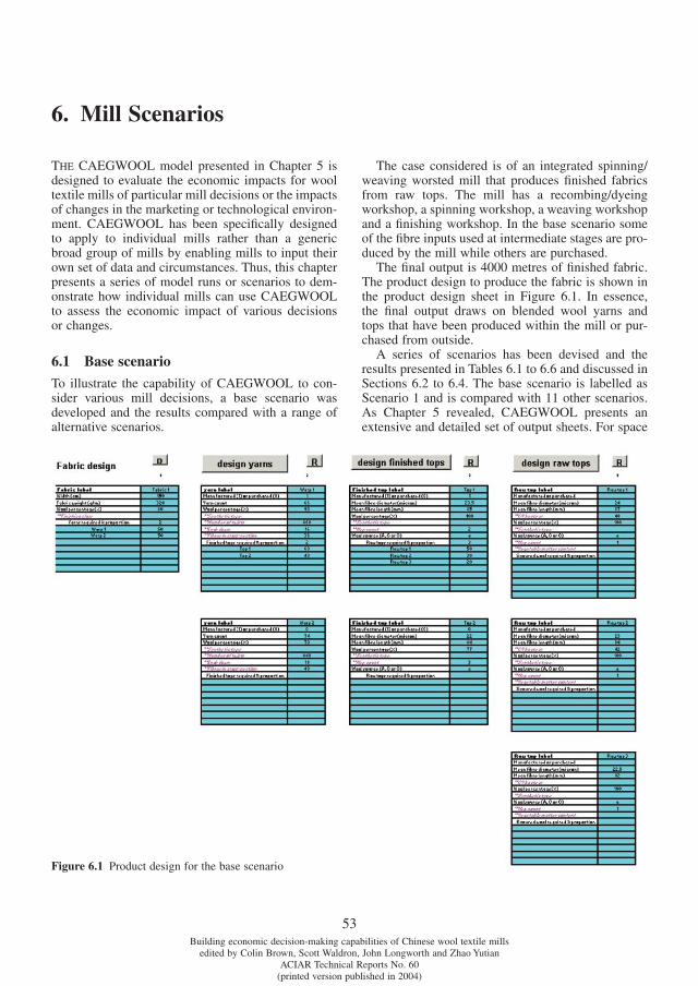
53Building economic decision-making capabilities of Chinese wool textile mills
edited by Colin Brown, Scott Waldron, John Longworth and Zhao YutianACIAR Technical Reports No. 60
(printed version published in 2004)
THE CAEGWOOL model presented in Chapter 5 is designed to evaluate the economic impacts for wool textile mills of particular mill decisions or the impacts of changes in the marketing or technological environ-ment. CAEGWOOL has been specifi cally designed to apply to individual mills rather than a generic broad group of mills by enabling mills to input their own set of data and circumstances. Thus, this chapter presents a series of model runs or scenarios to dem-onstrate how individual mills can use CAEGWOOL to assess the economic impact of various decisions or changes.
6.1 Base scenario
To illustrate the capability of CAEGWOOL to con-sider various mill decisions, a base scenario was developed and the results compared with a range of alternative scenarios.
The case considered is of an integrated spinning/weaving worsted mill that produces fi nished fabrics from raw tops. The mill has a recombing/dyeing workshop, a spinning workshop, a weaving workshop and a fi nishing workshop. In the base scenario some of the fi bre inputs used at intermediate stages are pro-duced by the mill while others are purchased.
The fi nal output is 4000 metres of fi nished fabric. The product design to produce the fabric is shown in the product design sheet in Figure 6.1. In essence, the fi nal output draws on blended wool yarns and tops that have been produced within the mill or pur-chased from outside.
A series of scenarios has been devised and the results presented in Tables 6.1 to 6.6 and discussed in Sections 6.2 to 6.4. The base scenario is labelled as Scenario 1 and is compared with 11 other scenarios. As Chapter 5 revealed, CAEGWOOL presents an extensive and detailed set of output sheets. For space
6. Mill Scenarios
Figure 6.1 Product design for the base scenario
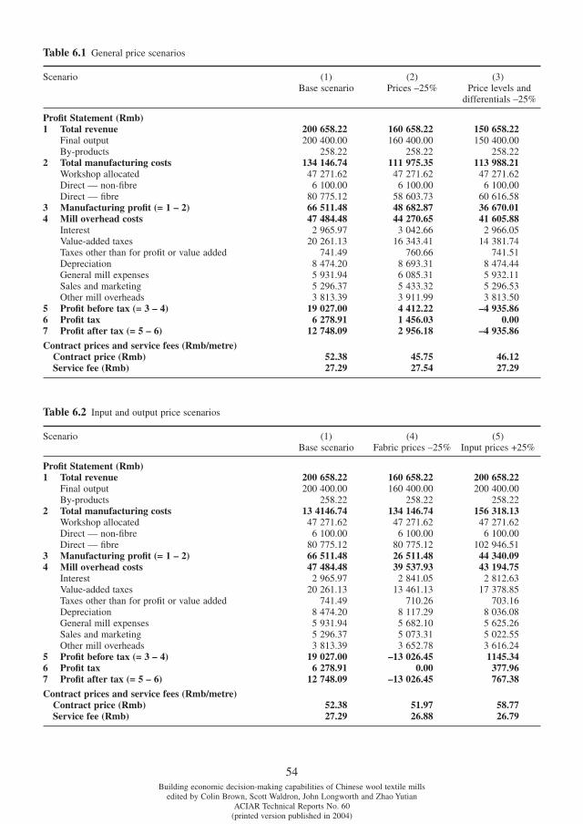
54Building economic decision-making capabilities of Chinese wool textile mills
edited by Colin Brown, Scott Waldron, John Longworth and Zhao YutianACIAR Technical Reports No. 60
(printed version published in 2004)
Table 6.1 General price scenarios
Scenario (1)Base scenario
(2)Prices –25%
(3) Price levels and
differentials –25%
Profi t Statement (Rmb)1 Total revenue 200 658.22 160 658.22 150 658.22
Final output 200 400.00 160 400.00 150 400.00By-products 258.22 258.22 258.22
2 Total manufacturing costs 134 146.74 111 975.35 113 988.21Workshop allocated 47 271.62 47 271.62 47 271.62Direct — non-fi bre 6 100.00 6 100.00 6 100.00Direct — fi bre 80 775.12 58 603.73 60 616.58
3 Manufacturing profi t (= 1 – 2) 66 511.48 48 682.87 36 670.014 Mill overhead costs 47 484.48 44 270.65 41 605.88
Interest 2 965.97 3 042.66 2 966.05Value-added taxes 20 261.13 16 343.41 14 381.74Taxes other than for profi t or value added 741.49 760.66 741.51Depreciation 8 474.20 8 693.31 8 474.44General mill expenses 5 931.94 6 085.31 5 932.11Sales and marketing 5 296.37 5 433.32 5 296.53Other mill overheads 3 813.39 3 911.99 3 813.50
5 Profi t before tax (= 3 – 4) 19 027.00 4 412.22 –4 935.866 Profi t tax 6 278.91 1 456.03 0.007 Profi t after tax (= 5 – 6) 12 748.09 2 956.18 –4 935.86
Contract prices and service fees (Rmb/metre) Contract price (Rmb) 52.38 45.75 46.12 Service fee (Rmb) 27.29 27.54 27.29
Table 6.2 Input and output price scenarios
Scenario (1)Base scenario
(4)Fabric prices –25%
(5)Input prices +25%
Profi t Statement (Rmb)1 Total revenue 200 658.22 160 658.22 200 658.22
Final output 200 400.00 160 400.00 200 400.00By-products 258.22 258.22 258.22
2 Total manufacturing costs 13 4146.74 134 146.74 156 318.13Workshop allocated 47 271.62 47 271.62 47 271.62Direct — non-fi bre 6 100.00 6 100.00 6 100.00Direct — fi bre 80 775.12 80 775.12 102 946.51
3 Manufacturing profi t (= 1 – 2) 66 511.48 26 511.48 44 340.094 Mill overhead costs 47 484.48 39 537.93 43 194.75
Interest 2 965.97 2 841.05 2 812.63Value-added taxes 20 261.13 13 461.13 17 378.85Taxes other than for profi t or value added 741.49 710.26 703.16Depreciation 8 474.20 8 117.29 8 036.08General mill expenses 5 931.94 5 682.10 5 625.26Sales and marketing 5 296.37 5 073.31 5 022.55Other mill overheads 3 813.39 3 652.78 3 616.24
5 Profi t before tax (= 3 – 4) 19 027.00 –13 026.45 1145.346 Profi t tax 6 278.91 0.00 377.967 Profi t after tax (= 5 – 6) 12 748.09 –13 026.45 767.38
Contract prices and service fees (Rmb/metre) Contract price (Rmb) 52.38 51.97 58.77 Service fee (Rmb) 27.29 26.88 26.79
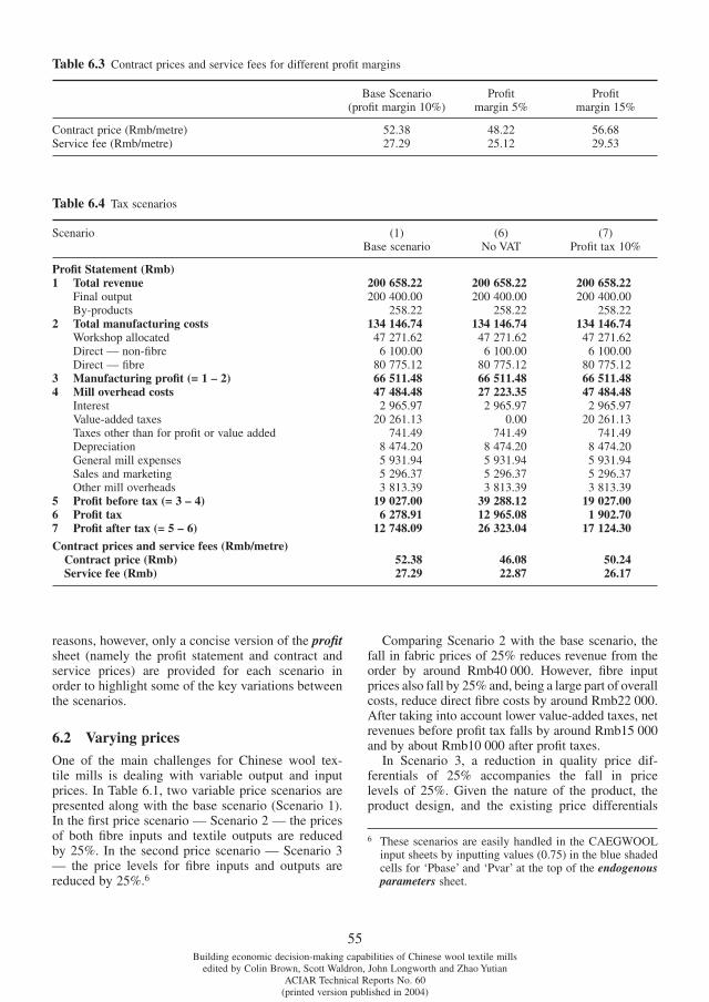
55Building economic decision-making capabilities of Chinese wool textile mills
edited by Colin Brown, Scott Waldron, John Longworth and Zhao YutianACIAR Technical Reports No. 60
(printed version published in 2004)
reasons, however, only a concise version of the profi t sheet (namely the profi t statement and contract and service prices) are provided for each scenario in order to highlight some of the key variations between the scenarios.
6.2 Varying prices
One of the main challenges for Chinese wool tex-tile mills is dealing with variable output and input prices. In Table 6.1, two variable price scenarios are presented along with the base scenario (Scenario 1). In the fi rst price scenario — Scenario 2 — the prices of both fi bre inputs and textile outputs are reduced by 25%. In the second price scenario — Scenario 3 — the price levels for fi bre inputs and outputs are reduced by 25%.6
Comparing Scenario 2 with the base scenario, the fall in fabric prices of 25% reduces revenue from the order by around Rmb40 000. However, fi bre input prices also fall by 25% and, being a large part of overall costs, reduce direct fi bre costs by around Rmb22 000. After taking into account lower value-added taxes, net revenues before profi t tax falls by around Rmb15 000 and by about Rmb10 000 after profi t taxes.
In Scenario 3, a reduction in quality price dif-ferentials of 25% accompanies the fall in price levels of 25%. Given the nature of the product, the product design, and the existing price differentials
Table 6.3 Contract prices and service fees for different profi t margins
Base Scenario(profi t margin 10%)
Profi tmargin 5%
Profi tmargin 15%
Contract price (Rmb/metre) 52.38 48.22 56.68Service fee (Rmb/metre) 27.29 25.12 29.53
Table 6.4 Tax scenarios
Scenario (1)Base scenario
(6)No VAT
(7)Profi t tax 10%
Profi t Statement (Rmb)1 Total revenue 200 658.22 200 658.22 200 658.22
Final output 200 400.00 200 400.00 200 400.00By-products 258.22 258.22 258.22
2 Total manufacturing costs 134 146.74 134 146.74 134 146.74Workshop allocated 47 271.62 47 271.62 47 271.62Direct — non-fi bre 6 100.00 6 100.00 6 100.00Direct — fi bre 80 775.12 80 775.12 80 775.12
3 Manufacturing profi t (= 1 – 2) 66 511.48 66 511.48 66 511.484 Mill overhead costs 47 484.48 27 223.35 47 484.48
Interest 2 965.97 2 965.97 2 965.97Value-added taxes 20 261.13 0.00 20 261.13Taxes other than for profi t or value added 741.49 741.49 741.49Depreciation 8 474.20 8 474.20 8 474.20General mill expenses 5 931.94 5 931.94 5 931.94Sales and marketing 5 296.37 5 296.37 5 296.37Other mill overheads 3 813.39 3 813.39 3 813.39
5 Profi t before tax (= 3 – 4) 19 027.00 39 288.12 19 027.006 Profi t tax 6 278.91 12 965.08 1 902.707 Profi t after tax (= 5 – 6) 12 748.09 26 323.04 17 124.30
Contract prices and service fees (Rmb/metre) Contract price (Rmb) 52.38 46.08 50.24 Service fee (Rmb) 27.29 22.87 26.17
6 These scenarios are easily handled in the CAEGWOOL input sheets by inputting values (0.75) in the blue shaded cells for ‘Pbase’ and ‘Pvar’ at the top of the endogenous parameters sheet.
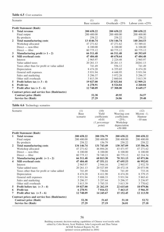
56Building economic decision-making capabilities of Chinese wool textile mills
edited by Colin Brown, Scott Waldron, John Longworth and Zhao YutianACIAR Technical Reports No. 60
(printed version published in 2004)
Table 6.5 Cost scenarios
Scenario (1)Base scenario
(8)Overheads –25%
(9)Labour costs +25%
Profi t Statement (Rmb)1 Total revenue 200 658.22 200 658.22 200 658.22
Final output 200 400.00 200 400.00 200 400.00By-products 258.22 258.22 258.22
2 Total manufacturing costs 13 4146.74 134 146.74 140 264.53Workshop allocated 47 271.62 47 271.62 53 389.41Direct — non-fi bre 6 100.00 6 100.00 6 100.00Direct — fi bre 80 775.12 80 775.12 80 775.12
3 Manufacturing profi t (= 1 – 2) 66 511.48 66 511.48 60 393.694 Mill overhead costs 47 484.48 40 678.64 47 484.48
Interest 2 965.97 2 224.48 2 965.97Value-added taxes 20 261.13 20 261.13 20261.13Taxes other than for profi t or value added 741.49 556.12 741.49Depreciation 8 474.20 6 355.65 8 474.20General mill expenses 5 931.94 4 448.95 5 931.94Sales and marketing 5 296.37 3 972.28 5 296.37Other mill overheads 3 813.39 2 860.04 3 813.39
5 Profi t before tax (= 3 – 4) 19 027.00 25 832.84 12 909.216 Profi t tax 6 278.91 8 524.84 4 260.047 Profi t after tax (= 5 – 6) 12 748.09 17 308.00 8 649.17Contract prices and service fees (Rmb/metre) Contract price (Rmb) 52.38 49.95 54.57 Service fee (Rmb) 27.29 24.86 29.48
Table 6.6 Technology scenarios
Scenario (1)Base
scenario
(10)Yield
coeffi cients+0.01
(1 percentagepoint)
(11)Weaving costcoeffi cients
–25%;Workshop
depreciation+50 000
(12)Micron –1;
Hauteur–10 mm
Profi t Statement (Rmb)1 Total revenue 200 658.22 200 556.79 200 658.22 200 658.22
Final output 200 400.00 200 400.00 200 400.00 200 400.00By-products 258.22 156.79 258.22 258.22
2 Total manufacturing costs 134 146.74 131 743.49 130 347.09 135 586.36Workshop allocated 47 271.62 46 894.26 43 471.97 47 271.62Direct — non-fi bre 6 100.00 6 100.00 6 100.00 6 100.00Direct — fi bre 80 775.12 78 749.23 80 775.12 82 214.74
3 Manufacturing profi t (= 1 – 2) 66 511.48 68 813.30 70 311.13 65 071.864 Mill overhead costs 47 484.48 47 551.11 47 695.53 46 992.01
Interest 2 965.97 2 944.16 2 965.97 2 932.70Value-added taxes 20 261.13 20 527.89 20 472.18 20 073.98Taxes other than for profi t or value added 741.49 736.04 741.49 733.18Depreciation 8 474.20 8 411.90 8 474.20 8 379.15General mill expenses 5 931.94 5 888.33 5 931.94 5 865.41Sales and marketing 5 296.37 5 257.44 5 296.37 5 236.97Other mill overheads 3 813.39 3 785.35 3 813.39 3 770.62
5 Profi t before tax (= 3 – 4) 19 027.00 21 262.19 22 615.60 18 079.866 Profi t tax 6 278.91 7 016.52 7 463.15 5 966.357 Profi t after tax (= 5 – 6) 12 748.09 14 245.67 15 152.45 12 113.50Contract prices and service fees (Rmb/metre) Contract price (Rmb) 52.38 51.65 51.10 52.72 Service fee (Rmb) 27.29 27.19 26.01 27.18
57Building economic decision-making capabilities of Chinese wool textile mills
edited by Colin Brown, Scott Waldron, John Longworth and Zhao YutianACIAR Technical Reports No. 60
(printed version published in 2004)
between product types, an overall loss for the order of Rmb4935 arises. The main reason for the loss is the lower fabric price which results in a revenue of Rmb40 000 lower than the base scenario and Rmb10 000 lower than Scenario 2.
The scenarios in Table 6.1 assume that the prices for wool inputs and wool textile outputs follow the same patterns. Although a relationship between wool prices and wool textile prices can be expected, they also operate in quite distinct markets and are subject to different sets of supply and demand forces. For instance, wool prices are markedly affected by supply conditions and relative livestock product prices in the major wool-growing countries, while wool textile prices are governed primarily by consumer demand for apparel and other goods made from wool textiles. Thus, there have been numerous instances of wool textile prices moving independently of wool prices and vice versa. Scenarios 4 and 5 in Table 6.2 attempt to refl ect these independent price movements.
In Scenario 4, fabric prices fall by 25% but fi bre input prices remain the same. Compared with Scenario 2, the impact is quite marked. That is, reve-nues fall by Rmb40 000 but are not compensated for by a fall in fi bre input costs. Consequently, the overall impact is a loss on the order of Rmb13 026. Scenario 5 refl ects the situation that arose in 2002 where fabric prices remained virtually the same while wool input prices rose by 25%. The results in Table 6.2 indicate that direct fi bre costs rise to Rmb102 947 and result in a virtual break-even profi t after tax of Rmb767.
6.3 Contract prices and service fees
The bottom section of Tables 6.1 and 6.2 lists ‘con-tract prices’ and ‘service fees’ determined by CAEG-WOOL. These two items were defi ned in Section 5.2.4. Effectively the contract price is the price the mill needs to price the product in order to make a specifi ed after tax profi t or profi t margin. In the base scenario, along with all the other scenarios in Tables 6.1 to 6.2 and Tables 6.4 to 6.6, this margin is set at 10%. Thus, in arriving at the contract price, all costs including apportioned mill overheads and net value added tax are taken into account along with the profi t margin. The service fee is calculated in a similar manner to the contract price except that direct fi bre costs are excluded. That is, it presumes that the mill customer supplies the fi bre input and that the service fee represents all other costs for processing these fi bre inputs including the specifi ed profi t margin.
Table 6.3 presents contract prices and service fees (as determined by CAEGWOOL) for the base sce-nario for the standard 10% profi t margin as well as for profi t margins of 5% and 15%.7 Table 6.3 reveals that changing the profi t margin can have a marked
impact with contract prices varying from Rmb48.22 to Rmb56.68 and service fees from Rmb25.12 to Rmb29.53. The ability to identify or determine new contract prices or service fees as product design or other conditions change is a key output from the CAEGWOOL model and powerful tool for mill managers.
6.4 Varying taxes
The next set of scenarios considered and reported in Table 6.4 concerns varying taxes. There are a plethora of taxes that impact on the profi tability of wool tex-tile enterprises but the main taxes are the profi t tax and the value added tax. As a key model parameter in CAEGWOOL, the treatment of these taxes in the model is described in more detail in Section 5.2.4. In general, a value added tax applies to sales at a rate of 17% with a rebate able to be claimed on speci-fi ed inputs at a rate of 13%. A profi t tax rate of 33% normally applies to pre-(profi t) tax net revenues. However, in some circumstances usually related to products exported, an exemption to value added tax can apply. Similarly, although the profi t rate of 33% is widely applied, the rate is dependent on aggregate enterprise (as opposed to individual order) profi ts, and can be varied in other circumstances. Thus, there is a need to examine the sensitivity of the model results to changes in these key tax parameters.8
Scenario 6 in Table 6.4 presumes that no VAT on outputs or rebate on inputs applies. The impact in Table 6.4 is shown in Section 4 (‘Mill overhead costs’) of the Profi t Statement where combined value added taxes (tax on outputs minus rebate on inputs) is shown. Compared with the base scenario, the reduction in value added taxes increases profi t before (profi t) tax by around Rmb20 000. However, as profi t taxes are calculated after consideration of value added taxes, the increase in profi t after tax is less at around Rmb13 600.
In Scenario 7, profi t taxes are reduced from the standard 33% to 10%. This may refl ect the case of temporary tax relief support to a mill in a restruc-turing or transition phase. As shown in Table 6.4, the impact of this tax change is much less than the non-application of the value added taxes with taxes reduced (and profi ts increased) by around Rmb4400.
7 The alternative scenarios were run by simply changing the default value on the relevant blue shaded input cell (cell B38) on the price input sheet.
8 Provision is made on the price input sheet of the CAEG-WOOL model to change these default value added and profi t tax rates.
58Building economic decision-making capabilities of Chinese wool textile mills
edited by Colin Brown, Scott Waldron, John Longworth and Zhao YutianACIAR Technical Reports No. 60
(printed version published in 2004)
6.5 Cost scenarios
One of the major factors of concern to mill managers is the control of costs. This is a major reason behind the detailed disaggregation of costs by workshop and type in the CAEGWOOL output reporting. Thus, there are numerous cost scenarios that could be con-sidered, while the profi t statement in Table 6.5 does not reveal the extent of cost disaggregation available in CAEGWOOL. However, to illustrate how some of these alternative costs may impact on mill profi ta-bility, two cost scenarios are compared with the base scenario.
In Scenario 8, overhead costs are reduced by 25%.9 This may occur in a restructuring situation where an individual mill is brought into a group structure and where there may be cost economies for particular overheads.10 The impact manifests itself in Table 6.5 in Section 4 of the profi t statement with profi ts rising in this particular case by around Rmb4600.
Scenario 9 involves an increase in (non- managerial) labour costs of 25%. This may refl ect growing economic opportunities and rise in wages for unskilled labour for wool textile mills in indus-trial east coast regions.11 Because labour costs are a major proportion of all workshop allocated costs, the impact of the rise in labour costs in this partic-ular case is similar to that of the change in overheads except in the opposite direction — namely profi ts around Rmb4000 lower than the base scenario.
6.6 Technical scenarios
Wool textile mills have sought to improve their prof-itability through the uptake of new technology and equipment and an improvement in operational prac-tices. New technologies can impact in a number of ways: by reducing manufacturing costs; by increasing yields; or by combinations of increasing costs and increasing yields. Many new technologies involve substantial investments and have a number
of impacts, making an economic assessment compli-cated. CAEGWOOL is designed to assist managers with this economic assessment.
Many different technical decisions warranting an economic assessment and of interest to mill man-agers could be identifi ed. However, Table 6.6 pro-vides a sample of just three scenarios. In Scenario 10, processing yields for all stages were increased by one percentage point.12 As shown in Table 6.6, the higher yields reduce both the direct fi bre costs (less fi bre inputs are required to produce the order) as well as workshop allocated costs (as less fi bre input has to be processed). Furthermore, mill overhead costs for the order are also reduced as the order now takes proportionately less of overall mill activity with the rising yields.
Scenario 11 presents the case of new equipment which may lower manufacturing costs but increase depreciation costs associated with the purchase of the new equipment.13
Scenario 12 relates more to fi bre input/textile product selection than to technology per se. That is, there are a number of fi bre input combinations that can produce a particular wool textile output. Spin-ning prediction models and ACIAR research such as that carried out in project AS1/1997/70 are designed to assist mills identify some of these combinations. Mills also draw on experience and other sources to identify the different product designs. The CAEG-WOOL model can then assess the profi tability and cost implications associated with the different product design. In the hypothetical case used in Sce-nario 12, product design was changed by having tops that were 1 micron fi ner to compensate for their hau-teur being reduced by 1 cm.14 Although the profi t statement in Table 6.6 highlights the impact of this change, the full CAEGWOOL output is needed to observe the full range of impacts that this change in product design would have.
12 This was achieved by entering the new yields in the rel-evant blue shaded cells in Section 3 of the endogenous parameters sheet.
13 This scenario was achieved by entering new values for the cost coeffi cients in the relevant blue shaded cells in Section 2 of the endogenous parameters sheet while at the same time increasing the overheads for weaving in Section 2 of the cost input sheet.
14 The scenario was achieved by changing the param eters on the product design sheet, re-running the CREATE INPUT SHEETS, and then running the CREATE OUTPUT SHEETS.
9 This scenario was set up by changing the values in the blue shaded cells on the overhead cost coeffi cients sheet to 0.25.
10 Not all restructuring will reduce overheads. Situations of cumbersome management and governance structures combined with a desire to cross-subsidise losses within the group may potentially lead to overheads for some mills to increase.
11 The rise in wages may be more than 25% as improved labour productivity and effi ciency may partly offset rising wages.
59Building economic decision-making capabilities of Chinese wool textile mills
edited by Colin Brown, Scott Waldron, John Longworth and Zhao YutianACIAR Technical Reports No. 60
(printed version published in 2004)
CHINESE wool textile mills find themselves in the midst of a transition that includes changing owner-ship and governance structures, upgrading equipment and technology, and improving managerial and oper-ational practices and analytic capabilities. Many mills are only now addressing the latter phase of transi-tion and are seeking ways to effectively go about the process.
The remarkable ability of the Chinese economy and industry to adapt and change means that many of the current problems besetting the industry will undoubtedly be resolved in the future and a more robust and sophisticated industry can be expected. However, this does not mean that the transformation will be quick or smooth, or that enterprises cannot be assisted within this extremely dynamic environment.
In this rapidly changing environment, the pres-entation of one-off fi ndings may be of limited value. Changing relative prices and cost structures can quickly outdate a static analysis. Furthermore, Chinese wool textile mills exhibit enormous diver-sity in sizes, structures, technology and operational
practices. Thus, the series of analyses and models discussed in this report have been designed to be fl exible and to be tailored to individual mills. Much of the emphasis has been on describing or illustrating the approach so that mills can apply the approach or model to their own set of circumstances.
To facilitate the adoption of the approaches by indi-vidual enterprises, the data requirements and output reporting associated with these approaches have been based around the information and processing systems that mills are familiar with now. However, as technology, processes and information systems change and become more sophisticated, there is also the need for these operational systems and decision-making aids to evolve. The emphasis in the report on explaining the approach is to encourage and enable participants within the Chinese wool textile industry to refi ne, adapt, and develop these approaches as con-ditions and systems change in the future. The inten-tion has also been to provide a suffi ciently general and fl exible framework to facilitate the development of these models and analyses.
7. Conclusions
Angel, C., Stephen Beare and A.C. Zwart (1990), ‘Product Characteristics and Arbitrage in the Aus-tralian and New Zealand Wool Markets’, Australian Journal of Agricultural Economics, 34 (1), 67–79.
Brown, C.G. (1997), ‘Chinese Wool Auctions: Failed Agribusiness Reform or Future Marketing Channel?’, China Economic Review, 8 (2), 175–90.
Brown, C.G., Waldron, S.A. and Longworth, J.W. (2005), Modernizing China’s Industries: Lessons from Wool and Wool Textiles, Edward Elgar Publishing: Cheltenham UK.
Chinese Team Members of ACIAR Project 8811 (Ed.) (1994), Zhongguo Mianyang Yuanmao Shenchan Yu
Xiaoshou de Jingji Wenti (Economic Aspects of Raw Wool Production and Marketing in China), Zhongguo Mianyang Yuanmao Shenchan yu Xiaoshou de Jingji Wenti (Agricultural Scientech Publishing House of China): Beijing.
Longworth, J.W. and Brown, C.G. (1995), Agribusiness Reforms in China: The Case of Wool, CAB International: Wallingford, UK.
Longworth, J.W. and Williamson, G.J. (1993), China’s Pastoral Region: Sheep and Wool, Minority Nationalities, Rangeland Degradation and Sustainable Development, CAB International: Wallingford, UK.
References

![8: Cognitive Capabilities: Mental …itm/688/Wk5 - Mental Models...8: Cognitive Capabilities: Mental Representations, Problem Solving, and Decision Making [Ritter] There are several](https://img.pdfslide.net/doc/110x75/5b854d3e7f8b9aea498e1feb/8-cognitive-capabilities-mental-itm688wk5-mental-models8-cognitive-capabilities.jpg)