MASTER THESIS - 2012SECTION OF MICROENGINEERING

Building of a mobile robot:Sensing or Moving, Time and Energy.

Author: Louis SAINT-RAYMOND

Professor SFU: Richard VAUGHAN

Professor EPFL: Auke IJSPEERT

March 16, 2012

Abstract

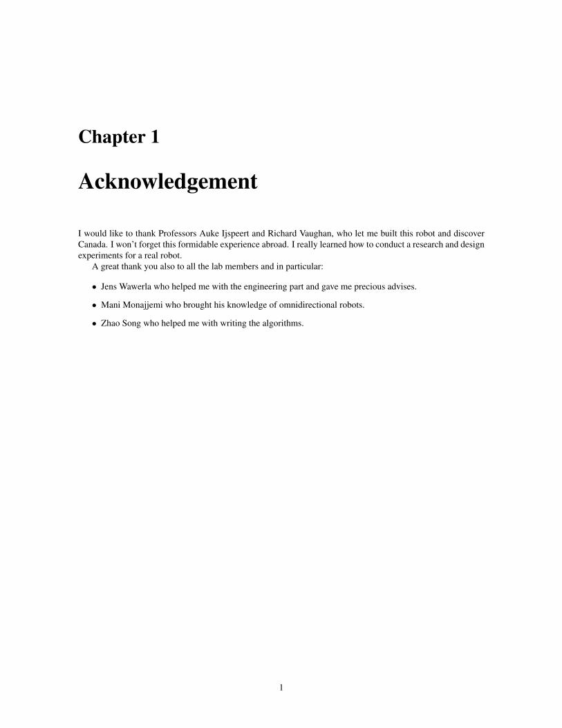
This thesis presents a new study of managing energy consumption in autonomous mobile robotics. A newrobot is developed in order to study the trade-off between gathering information about the surroundings andmoving efficiently to achieve a task. This robot has been designed with omnidirectional wheels to decouple therotation of the robot from the translation. A one laser beam distance sensor is embedded on the robot to acquireinformation, i.e. distance to obstacles. To explore the trade-off several behaviours of the robot are experimentedand the energy consumption and time are compared.

Chapter 1

Acknowledgement

I would like to thank Professors Auke Ijspeert and Richard Vaughan, who let me built this robot and discoverCanada. I won’t forget this formidable experience abroad. I really learned how to conduct a research and designexperiments for a real robot.

A great thank you also to all the lab members and in particular:

• Jens Wawerla who helped me with the engineering part and gave me precious advises.

• Mani Monajjemi who brought his knowledge of omnidirectional robots.

• Zhao Song who helped me with writing the algorithms.

1

Contents

1 Acknowledgement 1

2 Introduction 72.1 Energy management . . . . . . . . . . . . . . . . . . . . . . . . . . . . . . . . . . . . . . . . 72.2 Goal . . . . . . . . . . . . . . . . . . . . . . . . . . . . . . . . . . . . . . . . . . . . . . . . . 72.3 Related work . . . . . . . . . . . . . . . . . . . . . . . . . . . . . . . . . . . . . . . . . . . . 8

2.3.1 Autonomous mobile robots . . . . . . . . . . . . . . . . . . . . . . . . . . . . . . . . . 82.3.2 Range sensor . . . . . . . . . . . . . . . . . . . . . . . . . . . . . . . . . . . . . . . . 82.3.3 Omnidirectional robots . . . . . . . . . . . . . . . . . . . . . . . . . . . . . . . . . . . 8

2.4 Outlines . . . . . . . . . . . . . . . . . . . . . . . . . . . . . . . . . . . . . . . . . . . . . . . 9

3 Building of the robot 103.1 Choice of components . . . . . . . . . . . . . . . . . . . . . . . . . . . . . . . . . . . . . . . 10

3.1.1 Motors and wheels . . . . . . . . . . . . . . . . . . . . . . . . . . . . . . . . . . . . . 103.1.2 Laser Sensor . . . . . . . . . . . . . . . . . . . . . . . . . . . . . . . . . . . . . . . . 103.1.3 Processor and Inertial Measurement Unit . . . . . . . . . . . . . . . . . . . . . . . . . 113.1.4 Power sensor . . . . . . . . . . . . . . . . . . . . . . . . . . . . . . . . . . . . . . . . 113.1.5 Regulators . . . . . . . . . . . . . . . . . . . . . . . . . . . . . . . . . . . . . . . . . 11

3.2 Assembly of the robot . . . . . . . . . . . . . . . . . . . . . . . . . . . . . . . . . . . . . . . . 123.2.1 Plate . . . . . . . . . . . . . . . . . . . . . . . . . . . . . . . . . . . . . . . . . . . . 123.2.2 Bracket . . . . . . . . . . . . . . . . . . . . . . . . . . . . . . . . . . . . . . . . . . . 123.2.3 Standoffs . . . . . . . . . . . . . . . . . . . . . . . . . . . . . . . . . . . . . . . . . . 133.2.4 Resistor . . . . . . . . . . . . . . . . . . . . . . . . . . . . . . . . . . . . . . . . . . . 133.2.5 Connectors . . . . . . . . . . . . . . . . . . . . . . . . . . . . . . . . . . . . . . . . . 143.2.6 Miscellaneous . . . . . . . . . . . . . . . . . . . . . . . . . . . . . . . . . . . . . . . 17

3.3 Diagrams . . . . . . . . . . . . . . . . . . . . . . . . . . . . . . . . . . . . . . . . . . . . . . 173.3.1 Power . . . . . . . . . . . . . . . . . . . . . . . . . . . . . . . . . . . . . . . . . . . . 173.3.2 Connections . . . . . . . . . . . . . . . . . . . . . . . . . . . . . . . . . . . . . . . . 183.3.3 Communications . . . . . . . . . . . . . . . . . . . . . . . . . . . . . . . . . . . . . . 18

3.4 Software . . . . . . . . . . . . . . . . . . . . . . . . . . . . . . . . . . . . . . . . . . . . . . . 183.4.1 Arduino . . . . . . . . . . . . . . . . . . . . . . . . . . . . . . . . . . . . . . . . . . . 183.4.2 Motors control . . . . . . . . . . . . . . . . . . . . . . . . . . . . . . . . . . . . . . . 183.4.3 UART . . . . . . . . . . . . . . . . . . . . . . . . . . . . . . . . . . . . . . . . . . . . 193.4.4 Laser . . . . . . . . . . . . . . . . . . . . . . . . . . . . . . . . . . . . . . . . . . . . 203.4.5 Power consumption . . . . . . . . . . . . . . . . . . . . . . . . . . . . . . . . . . . . . 223.4.6 IMU . . . . . . . . . . . . . . . . . . . . . . . . . . . . . . . . . . . . . . . . . . . . . 233.4.7 Main Loop . . . . . . . . . . . . . . . . . . . . . . . . . . . . . . . . . . . . . . . . . 23

3.5 Problems encountered . . . . . . . . . . . . . . . . . . . . . . . . . . . . . . . . . . . . . . . . 243.5.1 RobotKit . . . . . . . . . . . . . . . . . . . . . . . . . . . . . . . . . . . . . . . . . . 243.5.2 Robovero . . . . . . . . . . . . . . . . . . . . . . . . . . . . . . . . . . . . . . . . . . 243.5.3 Overo . . . . . . . . . . . . . . . . . . . . . . . . . . . . . . . . . . . . . . . . . . . . 24

2

4 Algorithms and behaviours 254.1 Simulation . . . . . . . . . . . . . . . . . . . . . . . . . . . . . . . . . . . . . . . . . . . . . . 254.2 Follow Wall . . . . . . . . . . . . . . . . . . . . . . . . . . . . . . . . . . . . . . . . . . . . . 254.3 Reality . . . . . . . . . . . . . . . . . . . . . . . . . . . . . . . . . . . . . . . . . . . . . . . . 26

5 Experiments and results 285.1 Power measurement . . . . . . . . . . . . . . . . . . . . . . . . . . . . . . . . . . . . . . . . . 285.2 Preliminary experiment . . . . . . . . . . . . . . . . . . . . . . . . . . . . . . . . . . . . . . . 285.3 Main experiment . . . . . . . . . . . . . . . . . . . . . . . . . . . . . . . . . . . . . . . . . . 305.4 Results . . . . . . . . . . . . . . . . . . . . . . . . . . . . . . . . . . . . . . . . . . . . . . . . 30

5.4.1 Time . . . . . . . . . . . . . . . . . . . . . . . . . . . . . . . . . . . . . . . . . . . . 315.4.2 Energy . . . . . . . . . . . . . . . . . . . . . . . . . . . . . . . . . . . . . . . . . . . 31

6 Work plan 35

7 Conclusion and future work 367.1 Conclusion . . . . . . . . . . . . . . . . . . . . . . . . . . . . . . . . . . . . . . . . . . . . . 367.2 Future work . . . . . . . . . . . . . . . . . . . . . . . . . . . . . . . . . . . . . . . . . . . . . 36

7.2.1 Robot . . . . . . . . . . . . . . . . . . . . . . . . . . . . . . . . . . . . . . . . . . . . 367.2.2 Software . . . . . . . . . . . . . . . . . . . . . . . . . . . . . . . . . . . . . . . . . . 367.2.3 Algorithm . . . . . . . . . . . . . . . . . . . . . . . . . . . . . . . . . . . . . . . . . . 37

A Appendix 40A.1 Robot’s specifications . . . . . . . . . . . . . . . . . . . . . . . . . . . . . . . . . . . . . . . . 40A.2 Schematics . . . . . . . . . . . . . . . . . . . . . . . . . . . . . . . . . . . . . . . . . . . . . 43A.3 Bill of materials . . . . . . . . . . . . . . . . . . . . . . . . . . . . . . . . . . . . . . . . . . . 47

3

List of Figures

2.1 Three successful autonomous mobile robots . . . . . . . . . . . . . . . . . . . . . . . . . . . . 8

3.1 RobotKit, includes motors, encoders, microcontroller, wheels and battery . . . . . . . . . . . . 113.2 Current and voltage sensor . . . . . . . . . . . . . . . . . . . . . . . . . . . . . . . . . . . . . 113.3 Noise due to the motors: up to 0.3V . . . . . . . . . . . . . . . . . . . . . . . . . . . . . . . . 123.4 Small board for the LDO . . . . . . . . . . . . . . . . . . . . . . . . . . . . . . . . . . . . . . 123.5 3D view of the designed parts . . . . . . . . . . . . . . . . . . . . . . . . . . . . . . . . . . . . 133.6 Bad quality of manufacture for the plate . . . . . . . . . . . . . . . . . . . . . . . . . . . . . . 133.7 Standoffs too long . . . . . . . . . . . . . . . . . . . . . . . . . . . . . . . . . . . . . . . . . . 143.8 The standoff is filed because of the board . . . . . . . . . . . . . . . . . . . . . . . . . . . . . 143.9 Laser connectors . . . . . . . . . . . . . . . . . . . . . . . . . . . . . . . . . . . . . . . . . . 153.10 Gumstix power connector . . . . . . . . . . . . . . . . . . . . . . . . . . . . . . . . . . . . . . 153.11 The connectivity of the Robovero . . . . . . . . . . . . . . . . . . . . . . . . . . . . . . . . . . 163.12 The power sensor and its connector . . . . . . . . . . . . . . . . . . . . . . . . . . . . . . . . . 173.13 The UART connector . . . . . . . . . . . . . . . . . . . . . . . . . . . . . . . . . . . . . . . . 173.14 Diagram of power connexions . . . . . . . . . . . . . . . . . . . . . . . . . . . . . . . . . . . 183.15 Diagram of the connections . . . . . . . . . . . . . . . . . . . . . . . . . . . . . . . . . . . . . 193.16 Diagram of the communications . . . . . . . . . . . . . . . . . . . . . . . . . . . . . . . . . . 203.17 Diagram of the code executed on Arduino . . . . . . . . . . . . . . . . . . . . . . . . . . . . . 213.18 Example of how to drive an omnidirectional robot . . . . . . . . . . . . . . . . . . . . . . . . . 213.19 Number and direction of each motor . . . . . . . . . . . . . . . . . . . . . . . . . . . . . . . . 223.20 Axes of the IMU . . . . . . . . . . . . . . . . . . . . . . . . . . . . . . . . . . . . . . . . . . 23

4.1 Default trajectory of the robot . . . . . . . . . . . . . . . . . . . . . . . . . . . . . . . . . . . 264.2 Two different corners . . . . . . . . . . . . . . . . . . . . . . . . . . . . . . . . . . . . . . . . 264.3 The algorithm of the follow-wall behavior . . . . . . . . . . . . . . . . . . . . . . . . . . . . . 27

5.1 Power consumption of the driving in a straight line for different base orientations . . . . . . . . 295.2 Histogram of the current measurements when the robot is driving straight . . . . . . . . . . . . 295.3 Result of the T-test for the comparison of different base orientations . . . . . . . . . . . . . . . 305.4 Arena used for the experiments . . . . . . . . . . . . . . . . . . . . . . . . . . . . . . . . . . . 305.5 Arena used for the experiments . . . . . . . . . . . . . . . . . . . . . . . . . . . . . . . . . . . 315.6 Result of the T-test for the comparison of the time to do one loop . . . . . . . . . . . . . . . . . 315.7 Result of the T-test for the comparison of the energy consumption to do one loop . . . . . . . . 325.8 Time per loop for different angles of rebound . . . . . . . . . . . . . . . . . . . . . . . . . . . 325.9 Energy per loop for different angles of rebound . . . . . . . . . . . . . . . . . . . . . . . . . . 335.10 Trajectory of the robot for an angle of rebound of 20 . . . . . . . . . . . . . . . . . . . . . . . 335.11 Trajectory of the robot for an angle of rebound of 70 . . . . . . . . . . . . . . . . . . . . . . . 34

4

List of Tables

3.1 Pros and cons of the robot . . . . . . . . . . . . . . . . . . . . . . . . . . . . . . . . . . . . . 103.2 Laser connector, meaning of the colors . . . . . . . . . . . . . . . . . . . . . . . . . . . . . . . 153.3 UART protocol . . . . . . . . . . . . . . . . . . . . . . . . . . . . . . . . . . . . . . . . . . . 19

5

Master Project, Microengineering, 2011-2012Mr. Louis SAINT-RAYMOND

Building of a mobile robot:Sensing or Moving, Time and Energy.

We will build a robot to explore the trade-off between getting information about the environment and mov-ing fast. Sensing the environment to interact with requires time, but is necessary for the robot to avoid obstaclesand find its path to reach a target. Driving straight forward allows the robot to move fast, on the other handrotating increases the field of view of the robot, which improves the detection of obstacles.

We will use a robot with four omni-directional wheels, to decouple the direction of the robot from itsorientation. A long range laser distance sensor will let the robot avoid obstacles. We will add an IMU tocompensate for the lack of odometry due to the omni-directional wheels ; and a microprocessor with Linuxembedded for more high-level and intensive computation and for a wireless communication. The robot willrotate to scan the environment, and will drive through the corridor, in order to complete a loop of our officebuilding.

With this configuration we can choose to drive fast with a small field of view, or acquire more informationsby rotating.

Figure 1: Sketch of the robot

The goals of the project are:

- Build a fast four holonomic wheeled robot.

- Control the robot with a one-ray laser distance sensor.

- Simulate the behavior of the robot.

- Apply the behavior on the real robot, in the corridor.

- Monitor the energy consumption and the time per lap.

References[1] Malcolm A. MacIver, Neelesh A. Patankar, and Anup A. Shirgaonkar. Energy-information trade-offs be-

tween movement and sensing. PLoS Comput Biol, 6(5):e1000769, 05 2010.

Professor SFU: Richard VAUGHAN, Autonomy Lab Professor EPFL: Auke IJSPEERT, Biorob

October 27, 2011

1

Chapter 2

Introduction

Mobile robotics is an active research field growing in commercial and residential use.

2.1 Energy managementAn important point in mobile robotics is energy management. To improve the run-time of a robot, increasing thesize of the battery is an easy solution, however this leads to a more expensive and heavier model. Accelerationis also impacted due to the robot’s weight. Moreover with an efficient energy management, the robot can covera wider range where it can perform more work. A study by Yongguo Mei et al. [1] outlines methods to reducethe energy consumption of the robot. Yongguo Mei et al. demonstrate the benefit of implementing DynamicPower Management techniques, like the shutdown of unused components or the sensing frequency scaling tosave up to fifty percent of the robot’s consumption. Another approach is to integrate the energy managementin the path planning, like the studies of Tianmio Wang et al. [2] and of Ooi and Schindelhauer [3]. The firstproposes path planning which guarantees the robot to stay alive and finish all tasks with the minimum energy.The second finds the path to optimize the energy consumption for mobility and wireless communication.

But when the robot runs out of energy, it needs to be recharged. In this context, Litus et al. [4] presentsolutions to the problem of finding an energy efficient route for a mobile recharge station to rendezvous withworker robots. Then in the frame of time discounted labour, Wawerla and Vaughan [5] study the question:how much energy should be stored before working? Since 2002, Melhuish et al. [6] have built three robotsusing Microbial Fuel cells to imitate animals which recharge themselves by eating organic ingredients. Theydemonstrated the feasibility of producing energy from chemical substance for a mobile robot.

Malcom et al. [7] studied the trade-off between motion and sensing performance as seen through the evolu-tion of a fish. In a trade-off between sensory performance and speed Malcom et al. suggest that a fish evolvedan inefficient swim in order to increase its prey rate detection. For researchers in robotics the same trade-offexists as we attempt to balance sensory performance and efficiency.

2.2 GoalThe goal of this project is to build an autonomous robot and explore the trade-off between gathering informationregarding its physical surroundings and moving efficiently. We will begin by designing and building the robotwith a fixed one beam distance sensor. Thus the robot will need to rotate to scan the surrounding environment,which consumes both time and energy. We will use omnidirectional wheels, to decouple the rotation fromthe translation, so that the robot can drive in one direction with the translation, while receiving informationabout another with the rotation. We will then initiate an experiment to study the trade-off between gatheringinformation and moving efficiently.

This thesis is a case study in autonomous mobile robotics where the results show that a robot with smallsensing capabilities needs a lot of behaviour to achieve a task.

7

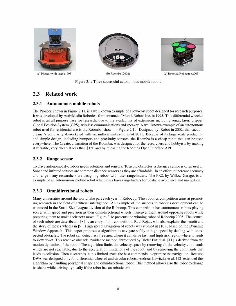
(a) Pioneer with laser (1995) (b) Roomba (2002) (c) Robot at Robocup (2005)

Figure 2.1: Three successful autonomous mobile robots

2.3 Related work

2.3.1 Autonomous mobile robotsThe Pioneer, shown in Figure 2.1a, is a well known example of a low-cost robot designed for research purposes.It was developed by ActivMedia Robotics, former name of MobileRobots Inc, in 1995. This differential wheeledrobot is an all purpose base for research, due to the availability of extensions including sonar, laser, gripper,Global Position System (GPS), wireless communications and speaker. A well known example of an autonomousrobot used for residential use is the Roomba, shown in Figure 2.1b. Designed by iRobot in 2002, this vacuumcleaner’s popularity skyrocketed with six million units sold as of 2011. Because of its large scale productionand simple design, including bumpers and proximity sensors, the Roomba is a cheap robot that can be usedeverywhere. The Create, a variation of the Roomba, was designed for the researchers and hobbyists by makingit versatile, very cheap at less than $150 and by releasing the Roomba Open Interface API.

2.3.2 Range sensorTo drive autonomously, robots needs actuators and sensors. To avoid obstacles, a distance sensor is often useful.Sonar and infrared sensors are common distance sensors as they are affordable. In an effort to increase accuracyand range many researchers are designing robots with laser rangefinders. The PR2, by Willow Garage, is anexample of an autonomous mobile robot which uses laser rangefinders for obstacle avoidance and navigation.

2.3.3 Omnidirectional robotsMany universities around the world take part each year in Robocup. This robotics competition aims at promot-ing research in the field of artificial intelligence. An example of the success in robotics development can bewitnessed in the Small Size League division of the Robocup. This competition has autonomous robots playingsoccer with speed and precision as their omnidirectional wheels maneuver them around opposing robots whilepreparing them to make their next move. Figure 2.1c presents the winning robot of Robocup 2005. The controlof such robots are described in [8] by an entry of this competition, Raul Rojas, who also explains the benefit andthe story of theses wheels in [9]. High speed navigation of robots was studied in [10] , based on the DynamicWindow Approach. This paper proposes a algorithm to navigate safely at high speed by dealing with unex-pected obstacles. The robot can detect risk free area where it can drive fast, and high risk region where it needsto slow down. This reactive obstacle avoidance method, introduced by Dieter Fox et al. [11] is derived from themotion dynamics of the robot. The algorithm limits the velocity space by removing all the velocity commandswhich are not reachable, due to the acceleration limitations of the robot, and by removing the commands thatleads to collision. Then it searches in this limited space the best commands to optimize the navigation. BecauseDWA was designed only for differential wheeled and circular robots, Andreas Lawitzky et al. [12] extended thisalgorithm by handling polygonal shape and omnidirectional robot. This method allows also the robot to changeits shape while driving, typically if the robot has an robotic arm.

8

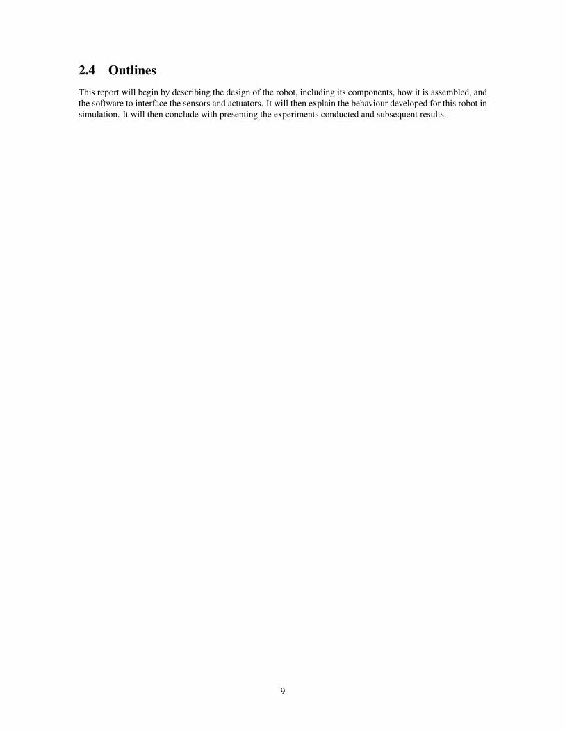
2.4 OutlinesThis report will begin by describing the design of the robot, including its components, how it is assembled, andthe software to interface the sensors and actuators. It will then explain the behaviour developed for this robot insimulation. It will then conclude with presenting the experiments conducted and subsequent results.

9

Chapter 3

Building of the robot

One objective of this project is to build a fast robot with a one beam distance sensor. This chapter will begin byrationalizing the decision behind using specific components, and the components’ function as it relates to theassembly and operation of the robot. The diagrams will then outline the different connections and the structureof the robot. This chapter will conclude with explaining the low-level software, how the sensors are read, andhow the motors are controlled.

3.1 Choice of componentsThis section describes the mechanical and electrical components of the robot, and justifies the reasons for usingthem.

3.1.1 Motors and wheelsAfter looking for each component separately, we found an pre-made omnidirectional platform, the RobotKit [13],shown in Figure 3.1. We decided to buy this unit to quickly get a functional robot and to have time to enhancethe software. As identified in the Table 3.1, the robot is slow, but the original gearbox (64:1) can be replacedwith one that has a ratio of approximatively 19:1. This will allow the robot to reach a maximum speed of 2m/s.Although the original motor is powerful, its torque will be reduced by three. The other downside of the robotis its weight.To reduce weight, we can replace the omnidirectional wheels with lighter ones reducing overallweight by 1kg. These two upgrades were not done in this project.

In addition to its pre-made omnidirectional platform, the robot has an electronic board and encoders tocontrol the motor, and a software to drive the unit. Specifications of the robot are in Appendix A.1.

Table 3.1: Pros and cons of the robot

Advantages DisadvantagesAlready built Slow (0.6m/s)

Encoders included Heavy (4kg)Robust and powerful

3.1.2 Laser SensorIn order for the robot to move quickly it needs a long-range sensor to detect obstacles. For an ultrasonic sensorthe refresh rate is too long due to the speed of the sound in the air, and infrared sensor has too short range.

At the beginning of the project, we wanted a fast (1kHz) and cheap laser distance sensor using triangulation,like this low cost range finder [14]. Consequently after researching the laser range finder, we concluded that it

10

Figure 3.1: RobotKit, includes motors, encoders, microcontroller, wheels and battery

would take too long to construct, and that it would be a challenge to achieve a long range due to the alignment ofthe camera and lens. No commercial product met our original requirement for a sensor based on triangulation.We decided to use a laser distance sensor based on time-of-flight, the VDM28-15 [15]. The maximum range ofthis sensor is 15m and the refresh rate is 100Hz.

3.1.3 Processor and Inertial Measurement UnitWe found a board with 9-axis inertial sensors (accelerometer, gyrometer and magnetometer) and a powerfulmicrocontroller. This board is the Robovero from Gumstix [16]. The IMU allows the robot to recognize itsposition and orientation. This board has several analog inputs which allows us to read the laser and powersensors.

We decided to buy the Overo Fire COM [17]. This is a small board with a microprocessor ARMCortex−A8 and a Wifi chip. This board, which can be plug directly on the Robovero, lets us communicate with therobot wirelessly and increase performance. It can run Linux, thus Python scripts, which is beneficial for thedevelopment of the software.

3.1.4 Power sensorWe need to measure the power consumed by the robot. We bought a current and voltage sensor [18], which isconnected to battery. Figure 3.2 shows the sensor, which is read by Robovero. The sensor is built to measureup to 45A, thus is not very sensitive to the current of the robot, about 2A.

Figure 3.2: Current and voltage sensor

3.1.5 RegulatorsWhen testing the robot, we encountered the challenge of noise on the analog lines. The first reason for noisewas a result of a defect with the regulator of the Robovero. The second reason for noise was due to the power

11

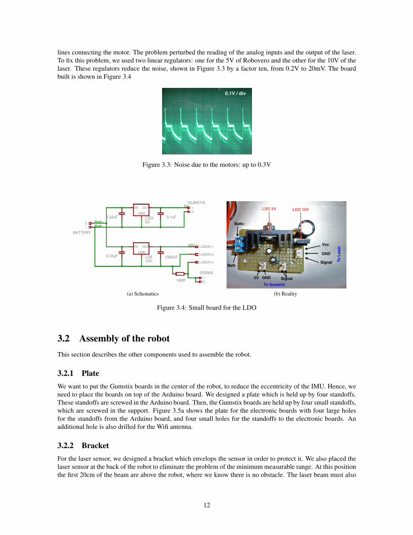
lines connecting the motor. The problem perturbed the reading of the analog inputs and the output of the laser.To fix this problem, we used two linear regulators: one for the 5V of Robovero and the other for the 10V of thelaser. These regulators reduce the noise, shown in Figure 3.3 by a factor ten, from 0.2V to 20mV. The boardbuilt is shown in Figure 3.4

0.1V / div

Figure 3.3: Noise due to the motors: up to 0.3V

(a) Schematics

Batt+

Batt-

5V GND Signal

Vcc

GND

Signal

LDO 5V LDO 10V

To Gumstix

To L

aser

(b) Reality

Figure 3.4: Small board for the LDO

3.2 Assembly of the robotThis section describes the other components used to assemble the robot.

3.2.1 PlateWe want to put the Gumstix boards in the center of the robot, to reduce the eccentricity of the IMU. Hence, weneed to place the boards on top of the Arduino board. We designed a plate which is held up by four standoffs.These standoffs are screwed in the Arduino board. Then, the Gumstix boards are held up by four small standoffs,which are screwed in the support. Figure 3.5a shows the plate for the electronic boards with four large holesfor the standoffs from the Arduino board, and four small holes for the standoffs to the electronic boards. Anadditional hole is also drilled for the Wifi antenna.

3.2.2 BracketFor the laser sensor, we designed a bracket which envelops the sensor in order to protect it. We also placed thelaser sensor at the back of the robot to eliminate the problem of the minimum measurable range. At this positionthe first 20cm of the beam are above the robot, where we know there is no obstacle. The laser beam must also

12

(a) Plate for the electronic boards (b) Bracket for the laser distancesensor

Figure 3.5: 3D view of the designed parts

pass above the electronic boards. The bracket is screwed in the base of the robot, and the laser sensor is hungby screws on the bracket. The Figure 3.5b shows this bracket for the laser sensor.

As shown in Figure 3.6, the quality of the plate was poor, however it did not affect the assembly of the robot.

Figure 3.6: Bad quality of manufacture for the plate

3.2.3 StandoffsFour standoffs are used to raise the plate above the Arduino board. The thread of the standoffs is too long (8mminstead of 4mm), but other lengths were not available. With the 8mm thread, the Arduino board is not properlyfastened. Hence, we have the choice between cutting the thread or adding some nuts and washers to get thenecessary length. We chose the second option, shown in Figure 3.7, because the first can damage the thread.One standoff is obstructed by the Arduino board, therefore we filed this standoff, as shown in Figure 3.8.

3.2.4 ResistorTo read the data of the laser, we use the analog output. The laser delivers a current between 4 and 20mA,proportional to the distance. We use a resistor to convert the current in voltage, and the microcontroller of theRobovero processes this information. The maximum input voltage of the microcontroller is 3.3V . The resistor

13

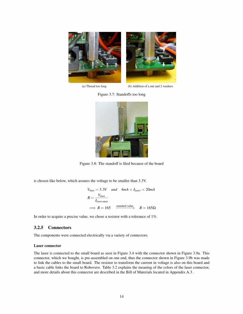
(a) Thread too long (b) Addition of a nut and 2 washers

Figure 3.7: Standoffs too long

Figure 3.8: The standoff is filed because of the board

is chosen like below, which assures the voltage to be smaller than 3.3V.

Vmax = 3.3V and 4mA < Ilaser < 20mA

R =Vmax

Ilaser,max

=⇒ R = 165 standard value−−−−−−−→ R = 165Ω

In order to acquire a precise value, we chose a resistor with a tolerance of 1%.

3.2.5 ConnectorsThe components were connected electrically via a variety of connectors.

Laser connector

The laser is connected to the small board as seen in Figure 3.4 with the connector shown in Figure 3.9a. Thisconnector, which we bought, is pre-assembled on one end, thus the connector shown in Figure 3.9b was madeto link the cables to the small board. The resistor to transform the current in voltage is also on this board anda basic cable links the board to Robovero. Table 3.2 explains the meaning of the colors of the laser connector,and more details about this connector are described in the Bill of Materials located in Appendix A.3 .

14

Table 3.2: Laser connector, meaning of the colors

Number Color Signal1 Brown Vcc2 White Analog output3 Blue GND4 Black LED in flashing mode

(a) Laser connector

Pin 4

Vcc

GND

Signal

(b) Laser connector1

Figure 3.9: Laser connectors

Gumstix power connector

Figure 3.10 shows the connector which transmits power from the LDO, shown in Figure 3.4 to Robovero. Figure3.11 shows where this connector is attached.

5VGNDGND5V

Figure 3.10: Gumstix power connector

Power consumption

To know the power consumption of the robot, we need to measure the current drawn off the battery and itsvoltage. Figure 3.12 shows the power sensor and its connector, with two cables for the voltage and the current,plus an additional cable, GND, used to have the same reference.

15

Tx1Rx1.

.

.GND

UART

AD0_2AD0_3.

AD0_0.

GND

.

.5V

AnalogPower

.

.GND

(a) In details

Power UART Analog

(b) With the connectors plugged

Figure 3.11: The connectivity of the Robovero

16

Ground

Current

Voltage

Figure 3.12: The power sensor and its connector

UART

For the UART communication between the Arduino and the Robovero, we used three wires, Tx to send, Rx toreceive, and GND to have the same reference. The connector is shown in Figure 3.13.

Robovero Arduino

Rob. Tx Rob RxArduino Tx,plug into D1

Arduino Rx, plug into D0

Figure 3.13: The UART connector

3.2.6 MiscellaneousAll the other components, such as screws, nuts, washers, etc. are listed in the Bill of Materials, in Appendix A.3.This includes the technical name of components, their quantity, mass, price and link to the manufacturer andreseller websites.

We used metric threads for the standoffs because the threads on the RobotKit were already metric, but wealso bought screws with imperial threads because in Canada it was cheaper and more readily available.

3.3 DiagramsThis section presents different diagrams to explain how the robot works.

3.3.1 PowerDiagram 3.14 shows the energy distribution of the robot. These values are the maximum values. In fact, duringour experiments, we observed a power consumption of 7.5W for the Gumstix boards, whose 5W are lost in heat

17

by the LDO, 2W for the laser and 12W for the motors.

Figure 3.14: Diagram of power connexions

3.3.2 ConnectionsDiagram 3.15 indicates where are plugged the cables and connectors.

3.3.3 CommunicationsDiagram 3.16 represents the communication between the components of the robot.

3.4 SoftwareTo transmit data, we do not only need cables, but we also need to write some code to understand the datareceived.

3.4.1 ArduinoFigure 3.17 presents the diagram of the code executed on Arduino. It indicates the time taken by each functionand the time between two calls of the function. We can see on the diagram that we can reach a loop time of6ms, corresponding to 160Hz, above the goal frequency of 100Hz. A LED is blinking to see if the program isrunning.

3.4.2 Motors controlThe main task of the microcontroller on Arduino is to control each motor to drive the robot as expected byRobovero. The microcontroller transforms the speed, rotational speed and direction given by Robovero in thefour speeds of the wheels. Figure 3.18 explains the idea of how to drive an omnidirectional robot by showingfour cases. The paper [8] shows how to compute the speed of the wheels from the speed of the robot.

The formula adapted to the RobotKit is presented below, where the speed of the wheels is on the left andthe speed and rotational speed of the robot are on the right. The angle ϕ is the angle of the wheels and is equalto 45 for the RobotKit. Figure 3.19 shows how the motors are numbered.

18

Figure 3.15: Diagram of the connections

Then we check that the maximum speed is not exceeded. If so, every speed is reduced by the same factor sothat each wheel is below the maximum speed.

v1v2v3v4

=

vULvLLvLRvUR

=

sinϕ −cosϕ −1sinϕ cosϕ −1−sinϕ cosϕ −1−sinϕ −cosϕ −1

vx

vyRω

3.4.3 UARTThe Arduino board receives the commands of speed in m/s, rotational speed in rad/s and the orientation of therobot in radian from Robovero and sends to Robovero the odometry of the four wheels in mm (in mm becausethe speed is integer). We use a baudrate of 115200bps because it is a good trade-off between speed and qualityof the data. Furthermore, we do not need a fast communication and this baudrate is also very common. Theprotocol of our serial communication is given in Table 3.3:

Table 3.3: UART protocol

Speed Rotational speed Orientation EndExample: 3e dc 28 f6 3e 99 99 9a 3f 99 99 9a 45

Data: 0.43m/s 0.3rad/s 1.2radType: float float float uint

19

Figure 3.16: Diagram of the communications

Wheel 0 Wheel 1 Wheel 2 Wheel 3 EndExample: 2 a0 2 76 fe 5c ff 19 45

Data: 672mm 630mm -420mm -231mmType: int int int int uint

Speed: 4 bytes, float, the first byte sent is the most significant byte. Same characteristics for rotational speed andorientation.

Wheel 1: 2 bytes, int, the first byte sent is the most significant byte. Same characteristics for the other wheels.

End: 1 byte, 0x45 (=69 in ASCII)

3.4.4 LaserThe output of the laser is a current between 4mA (20cm) and 20mA (15m). With a resistor of 165Ω withtranslate this current in a voltage because the microcontroller can only measure a voltage. After the conversionby the 12 bits Analog to Digital Converter (ADC) of the Robovero, we get a value between 819 and 4095. Thenwe translate this integer in a distance in meter with the formula 3.1:

20

Figure 3.17: Diagram of the code executed on Arduino

Figure 3.18: Example of how to drive an omnidirectional robot

21

Batt

ery

1 UL 4 UR

3 LR2 LL

USB plug

X

Y

330mm

250mm

Figure 3.19: Number and direction of each motor

d =U−Umin

Umax−Umin· (dmax−dmin)+dmin (3.1)

with d : the distance in meterU : the value given by the ADCUmin and Umax : minimum and maximum value of the ADC, respectively 819 and 4095dmin and dmax : respectively 20cm and 15m

3.4.5 Power consumptionThe output of the power sensor are voltages between 0 and 3.3V. The values from the ADC are then translatedin voltage or current by the following formulas 3.2:

22

X

Y Z zx

YAcc & Mag Gyro

Figure 3.20: Axes of the IMU

Vbatt =U · Vmax

Umax·KV/V (3.2)

I =U · Vmax

Umax·KA/V

with Vbatt : the voltage of the battery in VoltI : the current drawn by the robot in AmpereUmax : maximum value of the ADC, 4095Vmax : maximum value of the voltage corresponding to Umax, 3.3VKV/V : Parameter of the voltage sensor, 242.3mV/V, meaning that the voltage sensor output

gives 242.3mV per Volt measuredKA/V : Parameter of the current sensor, 73.2mV/A, meaning that the current sensor output

gives 73.2mV per Ampere measured

3.4.6 IMUThe Inertial Measurement Unit is composed of three sensors:

1. a 3-axis accelerometer which gives the acceleration of the robot in three orthogonal directions.

2. a 3-axis gyrometer which gives the rotational speed of the robot in three orthogonal directions.

3. a 3-axis magnetometer which gives the components of the magnetic field in three orthogonal directions.

Figure 3.20 presents the directions of the axes of the IMU. To be able the read these sensors fast enough, weused the patch given by Andrew Gottemoller [19], and we modified it a little bit to fit my application.

3.4.7 Main LoopIn the program, this loop coordinates the different functionalities of the robot.

The loop starts with the reading of the sensors: odometry, laser distance, power consumption and IMU. Withthese data, the pose estimation of the robot is updated. Then the algorithm computes the next driving commandsto apply. Finally, the data are stored in a file and the driving commands are send to the motors.

The battery level is also checked, and if it is below 9V, the program stops the motors before exiting.The main loop is executed in about 22ms, corresponding to 45Hz. It is below the 100Hz expected, because

it takes a lot of time to communicate between Overo and Robovero.

23

3.5 Problems encounteredWe had experienced various problems with the Gumstix products, Robovero and Overo and the RobotKit.

3.5.1 RobotKit1. Documentation: The documentation was not complete. Schematics was given too late.

2. Power line: The power lines are very noisy, due to the motors. It affects all the analog inputs of the robot.

3. Pushbutton: The pushbutton to turn On/Off the robot failed. We had to buy a new one.

4. Battery: After few months, the battery was no longer able to last more than five minutes. We bought anew battery to replace the first one.

3.5.2 Robovero1. Gyroscope: The gyroscope did not give good data. The problem was that the value of a capacitor was

wrong (amazingly, the cause of the problem was found by an EPFL student). We had to send back tothe company the Robovero board in order that they repair the board. We also bought a new one to avoidlosing time.

2. ADC: Only one analog input of six was readable, and we need three of them,. The company gave us aworkaround which works but maybe with low performance.

3. Power supply: When Robovero is supplied by the battery at 12V, the power line are very noisy and soundcan be heard. The noise causes bad analog readings. This problem is not specific to our board. Thecompany discovered the problem with us, hence there is no solution for the moment.

3.5.3 Overo1. Boot: The internal memory does not boot, hence we need to use a SD/SDHC card.

2. Wifi: It was difficult to understand how to use the Wifi, and then it took us a long time to look in theforums and to try by ourself to have a Wifi enabled automatically after the boot.

3. IMU: The refresh rate of the IMU is low, because of the software. A patch is available to get higherfrequencies.

4. UART reception: We were able to send through UART, but not to receive. The company updated thePython code, and now we can receive.

24

Chapter 4

Algorithms and behaviours

4.1 SimulationWe use a 2D simulator, Stage 4 [20], to develop our algorithm and try several behaviours. In the simulation, weuse a simplified map of the office building, no dynamics are simulated, and the robot is only a square box witha one-ray distance sensor, with an update rate of 100Hz.

We thought about different behaviours:

1. Follow wall: the robot follows the wall by bouncing against a virtual wall parallel to the real wall. Theserebounds let the robot to obtain informations about the wall position.

2. The robot rotates slowly to have a precise map of the environment, then goes straight in the direction ofthe longest range. After driving a distance equal to the longest range, it stops and rotates again to choosethe next destination.

3. The robot is always moving and rotating. It moves in the direction of the longest range, but this directioncan be simultaneously updated because of the continuous scan.

We chose to develop the Follow Wall behaviour because it is a minimal algorithm which do not build a mapof the environment.

4.2 Follow WallI began the simulation with a behaviour where the robot follows the wall, while always keeping the sameheading. This is possible due to the omnidirectional wheels.

First, the robot rotates to find the wall. The minimum range indicates the perpendicular to the wall. Later,the robot will regularly estimate this perpendicular to keep the right heading, θo f f set .

Then, the robot follows the wall with a curved trajectory which rebounces against the wall when the range,determined by the laser sensor, is below a threshold, as shown in the Figure 4.1. The robot needs this trajectoryto estimate the perpendicular to the wall, which allows the robot to be in the right direction for the next curve,given by the following formula: direction = (π

2 −θo f f set)+θrebound . This estimation is given by the method ofthe least squares, because the robot assumes that the walls are flat. This estimation is necessary due to the noisein the odometry and in the distance sensor, and also to adapt the heading of the robot when there is a corner.

The robot detects that there is a corner when the range becomes suddenly high or low. It distinguishesbetween two different corners, explained in the Figure 4.2. For an inside, corner the robot goes back and rotatesuntil it has the correct heading. For an outside corner, the robot makes a curve to avoid the corner. Figure 4.3summarizes this algorithm.

The robot is programmed to follow the wall in one direction with the wall always to its right. The path therobot takes is determined based on its initial positioning to the corridor. If positioned on an interior wall therobot will move clockwise. Conversely, if positioned on an exterior wall the robot will move counterclockwise.

25

θoffset

Direction of the next curve

Estimation of the perpendicular to the wall

Heading of the robot

θrebound

Figure 4.1: Default trajectory of the robot

(a) Inside corner (b) Outside corner

Figure 4.2: Two different corners

4.3 RealityThere are two main differences between the simulation and reality.

First the program runs at 45 Hz instead of 100Hz, as explained in 3.4.7. This can be a issue if the maximumspeed of the robot is increased.

Second, the inertia of the robot and slippage were not simulated. When the radius of the rebound is small,the robot undergoes more changes of direction. Due to the inertia and slippage, there is a delay between thecommands and the real movement as detected by the laser.

26

Figure 4.3: The algorithm of the follow-wall behavior

27

Chapter 5

Experiments and results

This chapter describes the experiments conducted and subsequent results.

5.1 Power measurementThe power consumption of the robot should not depend on the battery voltage. However, the Linear Drop Outregulator (LDO) transforms the voltage in excess into heat. This loss is proportional to the battery level. Theconsequence of this problem is that the first trials consume more energy due to the battery being fully charged.In the experiments, we remove this bias mathematically by computing the power used by the robot as seen, withUBatt the battery voltage, ULDO = 5V the output voltage of the LDO and ILDO = 0.7A the current through theLDO (this value has been measured):

Power =UBatt − ILDO(UBatt −ULDO)

Power =UBatt −0.7(UBatt −5)

5.2 Preliminary experimentThe angle named offset is a parameter [0, π

2 ] of the behavior, shown in Figure 4.1 . Without this offset, therobot cannot see inside corners. Large values of this offset imply farther anticipation, but a small change inthe heading produces a large change in the distance. Furthermore, we ran our first experiment to verify if therobot’s consumption depends on its bearing. The robot drives in a straight line for five seconds with differentoffset, while the voltage and the current are recorded.

The results of this experiments are presented in Figure 5.1. We can see that the variance of power consump-tion is high, and thus it is difficult to interpret this graph. In order to exploit this chart, we want to perform aStudent’s T-test to see if the means are different. Figure 5.2 presents an histogram of the current. It shows thatthe distribution of the measurements can be well-approximated by a gaussian noise around the average value.With more than 500 samples, this approximation is also verified by the central limit theorem. Thus T-test canbe performed. If the probability returns by the T-test is below 0.05, it means that the means are different witha confidence of 95 percent. In the three T-test Figures 5.3, 5.6 and5.7, a value in red is a value above thisthreshold. In this case we cannot say that the means are different.The results of this test are given in Figure 5.3.This test shows that with a confidence of 95 percent all the means are different with the exception of 10 with20, 40 with 50 and 0 with 90, as shown on the Figure 5.1.

With the T-test and the graph, we see that 40 and 50 are the most efficient offset to drive the robot. Thereason is that to drive with an offset of 45, the robot needs only two motors, but with an offset of 0 the robotneeds four motors. This mechanical property explains also the symmetry of the graph 5.1.

This result and the fact that the robot can anticipate corners are two reasons to choose an offset of 45. Thus,the next experiment will use this offset.

28

Not different

Not different

Not different

Figure 5.1: Power consumption of the driving in a straight line for different base orientations

1.00 1.05 1.10 1.15 1.20 1.25 1.30 1.35

Current [A]

0

20

40

60

80

100

Figure 5.2: Histogram of the current measurements when the robot is driving straight

29

Figure 5.3: Result of the T-test for the comparison of different base orientations

Starting position

8m

7m

9m

Figure 5.4: Arena used for the experiments

5.3 Main experimentTo explore the trade-off between sensing and moving, we decided to vary the angle of the rebound,θrebound ,shown in Figure 4.1. This angle affects the shape of the rebound and the trajectory of the robot. We expect tosee a relation between the angle and the energy. Indeed with a smaller angle, the rebound is also small and givesthe robot less time to compute the wall estimation, and a larger rebound angle gives the robot more informationabout its position relative to the wall, but does not take the shortest path around the arena.

The arena, shown in Figure 5.5 has by six walls, four inside corners and one outside corner. Starting in a setposition, the robot will follow the wall for one loop. This is represented by the red circle in graph 5.5. This runwill be replicated ten times for each of the seven angles [0, 20, 35, 45, 55, 70, 90].

5.4 ResultsFigures 5.10 and 5.11 show the trajectory of the robot for two angels of rebound. We can see that the resultingbehaviors are different.

30

Starting position

Figure 5.5: Arena used for the experiments

Figure 5.6: Result of the T-test for the comparison of the time to do one loop

5.4.1 TimeFigure 5.8 presents the result of the experiment for the time comparison. We can see a trend which suggeststhat an angle of rebound at 70 is the best angle for this arena, but the variance is high. As in the preliminaryexperiment, we perform T-test to see if our hypothesis ”the mean of 70 is different from the others” is true.The results of the T-test are presented in Figure 5.6. The T-test show that the mean of 70 is different with 95percent of confidence from the others, except from 50 and 90. We interpret this result as the need for the robotto move a lot to compensate for the low performance of its sensor.

5.4.2 EnergyFigure 5.9 presents the result of the experiment for the energy comparison. We can see that the most efficientangles seem to be 20 and 70. We perform T-test to see if the means are different. The result of the test,presented in Figure 5.7, is that we cannot say that the means of 20 and of 70 are different, and that the meansof 70 is different from the other angles except 0 and 45. These conclusions show that we cannot say that theangle of rebound influences the energy consumption. An explanation could be that with a small angle the robotchanges its speed more often than with a large angle, which requires energy, but its trajectory is shorter. Finallythe advantage of a short trajectory may be cancelled by more acceleration.

With the results of both comparison, we conclude that to drive efficiently in this arena a large angle ofrebound is more suitable. As the energy consumption does not seem to be affected by this angle, it is preferableto arrive at destination sooner.

31

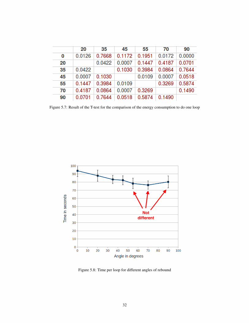
Figure 5.7: Result of the T-test for the comparison of the energy consumption to do one loop

Not different

Figure 5.8: Time per loop for different angles of rebound

32

Not different

Figure 5.9: Energy per loop for different angles of rebound

Figure 5.10: Trajectory of the robot for an angle of rebound of 20

33

Figure 5.11: Trajectory of the robot for an angle of rebound of 70

34

Chapter 6

Work plan

This chapter presents the work plan I followed during the project.

September: Definition of the project, search of components.

October: Start of the simulation, purchasing the components, start developing of the motor control with the RobotKit.

November: End of the motor control, implementation of the Follow Wall algorithm in simulation, drawing and order-ing of the bracket and the plate and all other additional components.

December: Familiarization with Gumstix boards, assembly of the robot, implementation of the communication be-tween the components.

Christmas: Deadline for the building of the robot

January: Reception of the laser, resolution of hardware and software problems.

February: Implementation of the Follow Wall algorithm on the real robot, start of the experiments.

March: Experiments and analysis and the results, writing of the thesis.

March, 15th: Deadline for mailing the thesis

April, 3rd : Oral defense of the thesis.

Because of the hardware and software problems, which took us a long time, we were late to implement thealgorithm on the real robot. Consequently, the robot began to follow the robot only at the end of February,which did not give us enough time to design other experiments.

35

Chapter 7

Conclusion and future work

7.1 ConclusionWe developed a new robot designed to explore the trade-off between gathering information about the surround-ings and moving efficiently. Although we were challenging by hardware’s or software’s difficulties, the buildingof the robot is a success. The results of our experiments shows that because of the small field of view of thesensor, the robot needs to increase its path to navigate efficiently.

Although the robot is working, few modifications are still possible to increase the performance of the robotand extend this study.

7.2 Future workThis chapter presents possible improvements of the robot’s hardware and software.

7.2.1 RobotThe robot could be improved with four modifications:

1. Wheels: The wheels of the robot could be replaced by lighter ones, like [21] to spare 1kg (25% of therobot’s weight).

2. Gearboxes: To increase the top speed of the robot, the ratio of the gearboxes could be increased from 1:64to 1:20. The torque would be also reduced.

3. Regulators: Currently, two linear regulators are used to supply Robovero and the laser. Linear regulatorsare easy to use, but not efficient. Switching regulators are more efficient models and will decrease thepower consumption.

4. Current sensor: The current sensor is designed to measure up to 45A. This sensor could be modified tohave a better sensibility to small current, by increasing the value of a resistor.

7.2.2 SoftwareThe frequency of the software is approximatively 40Hz. The bottleneck is the communication between Overoand Robovero.

One solution to increase the frequency is to have the algorithm on Overo running at a low frequency, andthe sensors reading and the communication with Arduino on Robovero running at a higher frequency. Howeverit is less convenient to write in C then compile, than to write Python scripts on Overo.

36

7.2.3 AlgorithmFirst, the correction of the robot’s bearing after a new estimation of the perpendicular to the wall could beexecuted while the robot is moving, because in the current implementation, the robot stops. It could lead toa more fluent and efficient behaviour. Second, other algorithms could be implemented to explore further thetrade-off between sensing and moving. I already proposed two others in the Chapter 4.

More pictures and movies of the robot are on the following website: http://www.sfu.ca/˜lsaintra/Louis_Saint-Raymond/. This project has also wiki notes on Github, with restricted access: https://github.com/AutonomyLab/wiki/wiki/Raymond.

37

Bibliography

[1] Yongguo Mei, Yung-Hsiang Lu, Y.C. Hu, and C.S.G. Lee. A case study of mobile robot’s energy consump-tion and conservation techniques. In Advanced Robotics, 2005. ICAR ’05. Proceedings., 12th InternationalConference on, pages 492 –497, july 2005.

[2] Tianmiao Wang, Bin Wang, Hongxing Wei, Yunan Cao, Meng Wang, and Zili Shao. Staying-alive andenergy-efficient path planning for mobile robots. In American Control Conference, 2008, pages 868 –873,june 2008.

[3] Chia Ching Ooi and Christian Schindelhauer. Minimal energy path planning for wireless robots. InProceedings of the 1st international conference on Robot communication and coordination, RoboComm’07, pages 2:1–2:8, Piscataway, NJ, USA, 2007. IEEE Press.

[4] Yaroslav Litus, Richard T. Vaughan, and Pawel Zebrowski. The frugal feeding problem: Energy-efficient,multi-robot, multi-place rendezvous. In Proceedings of the IEEE International Conference on Roboticsand Automation, April 2007.

[5] Jens Wawerla and Richard T. Vaughan. Optimal robot recharging strategies for time discounted labour. InProceedings of the Eleventh International Conference on the Simulation and Synthesis of Living Systems,Artificial Life, Winchester, UK, Aug. 2008.

[6] Ioannis Ieropoulos, Chris Melhuish, and John Greenman. Artificial metabolism: Towards true energeticautonomy in artificial life. In Wolfgang Banzhaf, Jens Ziegler, Thomas Christaller, Peter Dittrich, andJan Kim, editors, Advances in Artificial Life, volume 2801 of Lecture Notes in Computer Science, pages792–799. Springer Berlin / Heidelberg, 2003.

[7] Malcolm A. MacIver, Neelesh A. Patankar, and Anup A. Shirgaonkar. Energy-information trade-offsbetween movement and sensing. PLoS Comput Biol, 6(5):e1000769, 05 2010.

[8] Raul Rojas. Holonomic control of a robot with an omni-directional drive, 2006.

[9] Raul Rojas. A short history of omnidirectional wheels, 2006.

[10] Seokgyu Kim Woojin Chung and Jaesik Choi. High speed navigation of a mobile robot based on experi-ences. In The JSME Robotics and Mechatronics Conference (ROBOMEC 2006), May 2006.

[11] D. Fox, W. Burgard, and S. Thrun. The dynamic window approach to collision avoidance. RoboticsAutomation Magazine, IEEE, 4(1):23 –33, mar 1997.

[12] A. Lawitzky, D. Althoff, D. Wollherr, and M. Buss. Dynamic window approach for omni-directionalrobots with polygonal shape. In Robotics and Automation (ICRA), 2011 IEEE International Conferenceon, pages 2962 –2963, may 2011.

[13] NexusRobot. 4WD 100mm omni wheel mobile kit 10008. http://www.nexusrobot.com/product.php?id_product=66, consulted Oct 27, 2011.

[14] K. Konolige, J. Augenbraun, N. Donaldson, C. Fiebig, and P. Shah. A low-cost laser distance sensor. InRobotics and Automation, 2008. ICRA 2008. IEEE International Conference on, pages 3002 –3008, may2008.

38

[15] Pepperl+Fuchs. Laser distance sensor, vdm28-15. http://www.pepperl-fuchs.com/global/en/classid_53.htm?view=productdetails&prodid=48841, consulted Oct 28, 2011.

[16] Gumstix. Electronic board with microcontroller and inertial sensor. https://www.gumstix.com/store/product_info.php?products_id=262, consulted Oct 28, 2011.

[17] Gumstix. Computer on module with arm cortex-a8, wifi, bluetooth dsp. https://www.gumstix.com/store/product_info.php?products_id=227, consulted Oct 28, 2011.

[18] AttoPilot. Attopilot, voltage and current sensor. http://www.sparkfun.com/products/10643, con-sulted Nov 27, 2011.

[19] Andrew Gottemoller. Patch for imu on robovero. http://www.agottem.com/robovero_sensors, con-sulted Feb 2, 2012.

[20] Richard Vaughan. Massively multi-robot simulation in stage. Swarm Intelligence, 2(2):189–208, Decem-ber 2008.

[21] Kornilak. Omnidirectional wheel. http://store.kornylak.com/ProductDetails.asp?ProductCode=FXA165, consulted Feb 29, 2012.

39

Appendix A

Appendix

A.1 Robot’s specifications

40

Name: 4WD 100mm omni wheel learning kit 10008

Microcontroller Specification:Name of the boards: "Arduino IO Expansion", on top of the "Arduino 328 controller"ATmega328, recognize as Duemilanove or Nano w/ ATmega32814 digital input/output pins (6 can be used as PWM outputs)8 analog inputs16 MHz crystal oscillatorUSB connectionpower jackICSP headerreset buttonOperating Voltage: 5VInput Voltage (recommended): 7-12VInput Voltage (limits): 6-20VDigital I/O Pins: 14 (of which 6 provide PWM output)Analog Input Pins: 8DC Current per I/O Pin: 40 mADC Current for 3.3V Pin: 50 mAFlash Memory 32 KB of which 2KB used by bootloaderSRAM: 1KB(ATmega168) or 2KB(ATmega328)EEPROM:512bytes(ATmega168) or 1KB(ATmega328)Clock Speed: 16 MHz Motor:Motor Type: Faulhaber 12V DC Coreless Motor, 2342 L012CR, link, serial number:

2342 L012CR M124-Y2002 107, motor 12342 L012CR M124-Y2002 375, motor 22342 L012CR M124-Y2002 404, motor 32342 L012CR M124-Y2002 260, motor 4

Gearbox Ratio: 64:1, serial number:0715, gearbox 10546, gearbox 20445, gearbox 30705, gearbox 4

Power: 17WTorque: 16mNmMax speed 7000rpm Speed of the wheel: 120 rpm = 0.58m/s with Ø100mm wheelMax speed of the robot: 0.8m/sDiameter: 30mmLength: 85mmShaft Diameter: 6mmShaft Length: 35mmNo-Load Current: 75 mALoad Current: 1.4A

Encoder:Type: OpticalPhase: ABResolution: 12CPR, 768CPR of the wheel

Chassis Details:Length: 250mmWidth: 250mmCircumcircle diameter with wheels: 410mmHeight: 100mmGround clearance: 20mm with Ø100mm wheel

Net Weight: 4.00kgWheel Diameter: 100mmWheel Thickness: 38mmWheel Material: PolyurethaneWheel weight: 330gWheelbase: 260mmChassis Material: AluminumColor: YellowClimbing Capacity: 20 degree inclineLoad Capacity: 10kgController: Arduino ATMega328P, IO Expansion BoardPC104 Compatible: Yes

Battery and Charger:Battery: 12V NimH, 1800mAh, replaced by 2500mAhCharger: 100-240V IN, 2.4~12V OUT, 500mADuration of Charge: 2 hoursRunning time: 0.5 hours

Price: CAD 888.11Bought in 2011 on www.custobots.comContact: Markus Primbs, markus@custobots.comManufacturer: Nexus robot

A.2 Schematics

43

A.3 Bill of materials

47

Bill of materials

Part Name Number Mass [g] Power [W] Price [CAD] Website1 (manufacturer) Website2 (seller)

4WD Omni Wheel Learning PlatformDistance sensorVDM28-15-L-IO/73c/110/122RoboVero

Overo Fire COM

AttoPilot Voltage and Current Sense Breakout - 45A

M12 female angled 4pol. w/o LED 1,5m #21035154401#10-32 x 1-1/2" Round Head Slotted Square Combo Drive Machine Screw Zinc

SCREW MACHINE PHILLIPS 4-40X1/4STANDOFF HEX M3 THR ALUM 25MMNUT HEX 10-32 ZINC PLATEDNUT HEX 4-40 ZINC PLATED

KINGSTON 4GB MICROSD CARD WITH SD ADAPTERRES 165 OHM METAL FILM .60W 1%NiMH 2500mAh 12V, 10cellsIC REG LDO 1A 10V TO220FPIC REG 1A POS 5V

SWITCH PUSHBUTTON SPST 6A 14V

Total

RobotKit 1 4000 68.8 994.68 http://www.nexusrobot.net/product.php?id_product=66http://custobots.com/products/4wd-omni-wheel-learning-platform-10008Laser 1 90 2 509.54 http://www.pepperl-fuchs.com/global/en/classid_53.htm?view=productdetails&prodid=48841http://www.pepperl-fuchs.com/global/en/classid_53.htm?view=productdetails&prodid=48841IMU & uController 1 32.2 0.5 106 https://www.gumstix.com/store/product_info.php?products_id=262https://www.gumstix.com/store/product_info.php?products_id=262uProcessor 1 10 1 226 https://www.gumstix.com/store/product_info.php?products_id=227https://www.gumstix.com/store/product_info.php?products_id=227

Power sensor 1 23.67 http://www.sparkfun.com/products/10643Gumstix Plate 1 70 96.45 http://www.emachineshop.com/Laser bracket 1 200 132.595 http://www.emachineshop.com/Laser connector 1 50 18.35 http://www.harkis.harting.com/cgi-win/sbhtml.dll?crq_qs?&search=21035154401&language=ehttp://ca.mouser.com/ProductDetail/HARTING/21035154401/?qs=S64178dxKhd%252bo5OA2R1FLw%3d%3dScrew 10-32 1 1/2’’ 2 10.8 0.168 http://www.fastenal.com/web/products/detail.ex?sku=110161651&ucst=t

Screw 4-40 1/4’’ 4 10 0.1356 http://search.digikey.com/ca/en/products/PMS%20440%200025%20PH/H342-ND/49819Standoff M3 25mm 8 8.4 http://search.digikey.com/ca/en/products/24342/24342K-ND/1532143Nut 10-32 4 0.0896 http://search.digikey.com/ca/en/products/HNZ102/H228-ND/5741Nut 4-40 4 0.042 http://search.digikey.com/ca/en/products/HNZ440/H216-ND/5738Standoff #2 1/2’’ nylon round unthreaded4 In the Lab

Nuts 2-56 4 In the Lab

Screw 2-56 1/2’’, nylon 4 In the Lab

Cable In the Lab

Connector In the Lab

MicroSDHC 4Go 1 11.19 Kingston http://www.thesource.ca/estore/product.aspx?language=en-CA&catalog=Online&category=Memorycard_miniSD&product=4419305Resistor 165 1 0.35 http://search.digikey.com/ca/en/products/MRS25000C1650FRP00/PPC165ZCT-ND/594932Battery 1 68 http://www.buyabattery.com/DSE-SI-NH-AA2500R-C-V10A.pdfhttp://www.buyabattery.com/NiMH.htmlLDO 10V 1 1.91 http://www.rohm.com/products/databook/power/pdf/baxxbc0-e.pdfhttp://search.digikey.com/ca/en/products/BAJ0BC0T/BAJ0BC0T-ND/722291LDO 5V 1 http://www.fairchildsemi.com/ds/KA/KA7805E.pdfin the LabPushbutton 1 5.26 http://search.digikey.com/scripts/DkSearch/dksus.dll?x=0&y=0&lang=en&site=ca&KeyWords=gpb554dl05br

48 4'473 72.3 2'202.83