Building Scientific Data Solutions in Microsoft Azure and Microsoft Office 365

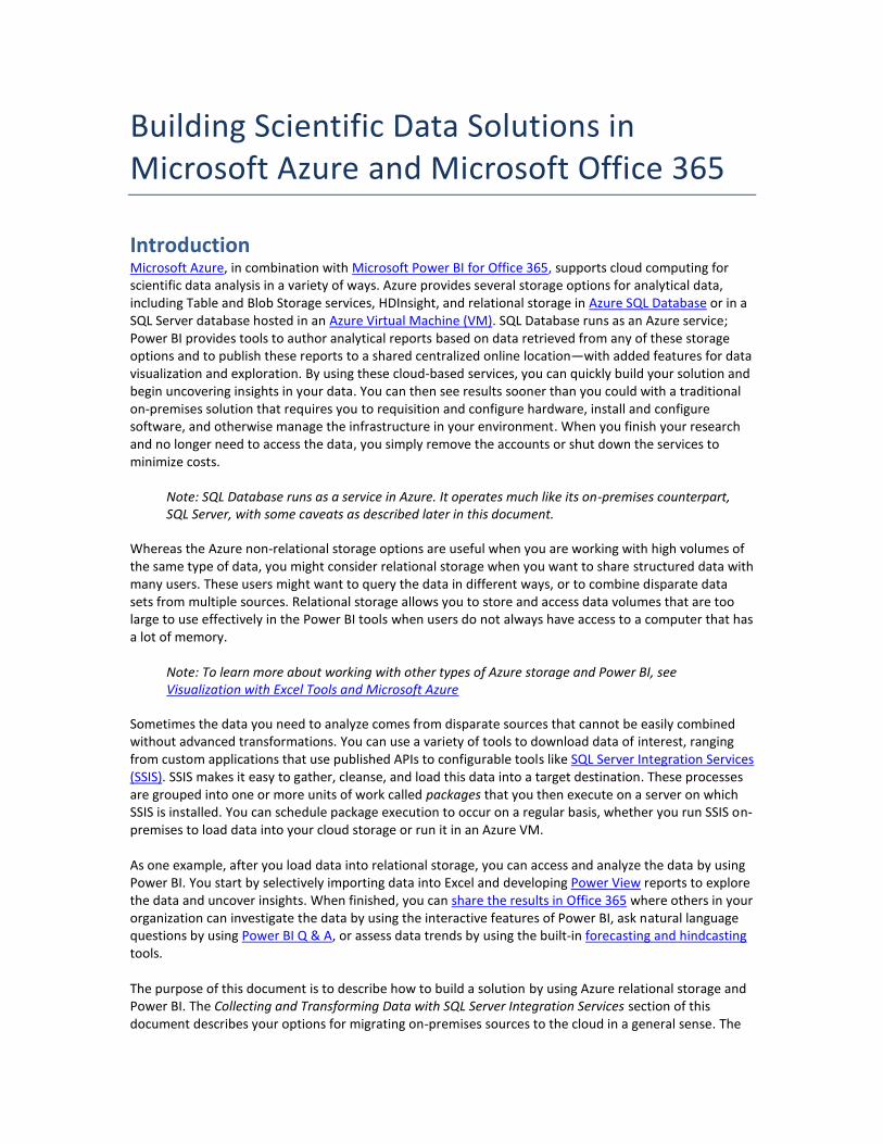
Introduction Microsoft Azure, in combination with Microsoft Power BI for Office 365, supports cloud computing for scientific data analysis in a variety of ways. Azure provides several storage options for analytical data, including Table and Blob Storage services, HDInsight, and relational storage in Azure SQL Database or in a SQL Server database hosted in an Azure Virtual Machine (VM). SQL Database runs as an Azure service; Power BI provides tools to author analytical reports based on data retrieved from any of these storage options and to publish these reports to a shared centralized online location—with added features for data visualization and exploration. By using these cloud-based services, you can quickly build your solution and begin uncovering insights in your data. You can then see results sooner than you could with a traditional on-premises solution that requires you to requisition and configure hardware, install and configure software, and otherwise manage the infrastructure in your environment. When you finish your research and no longer need to access the data, you simply remove the accounts or shut down the services to minimize costs.

Note: SQL Database runs as a service in Azure. It operates much like its on-premises counterpart, SQL Server, with some caveats as described later in this document.

Whereas the Azure non-relational storage options are useful when you are working with high volumes of the same type of data, you might consider relational storage when you want to share structured data with many users. These users might want to query the data in different ways, or to combine disparate data sets from multiple sources. Relational storage allows you to store and access data volumes that are too large to use effectively in the Power BI tools when users do not always have access to a computer that has a lot of memory.

Note: To learn more about working with other types of Azure storage and Power BI, see Visualization with Excel Tools and Microsoft Azure

Sometimes the data you need to analyze comes from disparate sources that cannot be easily combined without advanced transformations. You can use a variety of tools to download data of interest, ranging from custom applications that use published APIs to configurable tools like SQL Server Integration Services (SSIS). SSIS makes it easy to gather, cleanse, and load this data into a target destination. These processes are grouped into one or more units of work called packages that you then execute on a server on which SSIS is installed. You can schedule package execution to occur on a regular basis, whether you run SSIS on-premises to load data into your cloud storage or run it in an Azure VM. As one example, after you load data into relational storage, you can access and analyze the data by using Power BI. You start by selectively importing data into Excel and developing Power View reports to explore the data and uncover insights. When finished, you can share the results in Office 365 where others in your organization can investigate the data by using the interactive features of Power BI, ask natural language questions by using Power BI Q & A, or assess data trends by using the built-in forecasting and hindcasting tools. The purpose of this document is to describe how to build a solution by using Azure relational storage and Power BI. The Collecting and Transforming Data with SQL Server Integration Services section of this document describes your options for migrating on-premises sources to the cloud in a general sense. The

Building Scientific Data Solutions in Microsoft Azure and Microsoft Office 365

2

remainder of the document describes a scenario for capturing weather and crop data from publically available datasets that you can access by using FTP and HTTP protocols from the National Oceanic and Atmospheric Administration (NOAA) and the Food and Agriculture Organization of the United Nations (FAO), which you can subsequently integrate with your own research data. The examples in this document illustrate how to download historical average temperature data

1 (GZ file, 11.7 MB) and

associated country codes from NOAA in addition to historical crop production data by country2 (Excel file,

37.2 MB) from FOA. In addition, the examples show you how to cleanse and transform the data to prepare it for analysis, and then how to store it in a database.

Note: You can view documentation about the temperature data to learn how the data is structured in preparation for transforming and loading it into your database.

Choosing an Azure Architecture You can combine Azure services in several ways to design a cloud-based architecture for data storage that supports your data analysis:

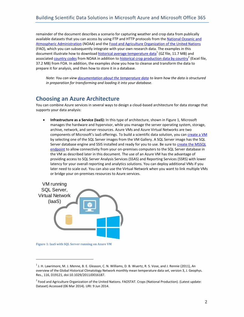
Infrastructure as a Service (IaaS): In this type of architecture, shown in Figure 1, Microsoft manages the hardware and hypervisor, while you manage the server operating system, storage, archive, network, and server resources. Azure VMs and Azure Virtual Networks are two components of Microsoft’s IaaS offerings. To build a scientific data solution, you can create a VM by selecting one of the SQL Server images from the VM Gallery. A SQL Server image has the SQL Server database engine and SSIS installed and ready for you to use. Be sure to create the MSSQL endpoint to allow connectivity from your on-premises computers to the SQL Server database in the VM as described later in this document. The use of an Azure VM has the advantage of providing access to SQL Server Analysis Services (SSAS) and Reporting Services (SSRS) with lower latency for your overall reporting and analytics solutions. You can deploy additional VMs if you later need to scale out. You can also use the Virtual Network when you want to link multiple VMs or bridge your on-premises resources to Azure services.

VM running

SQL Server,

Virtual Network

(IaaS)

Figure 1: IaaS with SQL Server running on Azure VM

1 J. H. Lawrimore, M. J. Menne, B. E. Gleason, C. N. Williams, D. B. Wuertz, R. S. Vose, and J. Rennie (2011), An

overview of the Global Historical Climatology Network monthly mean temperature data set, version 3, J. Geophys. Res., 116, D19121, doi:10.1029/2011JD016187.

2 Food and Agriculture Organization of the United Nations. FAOSTAT. Crops (National Production). (Latest update:

Dataset) Accessed (06 Mar 2014). URI: 9 Jun 2014.

Building Scientific Data Solutions in Microsoft Azure and Microsoft Office 365

3

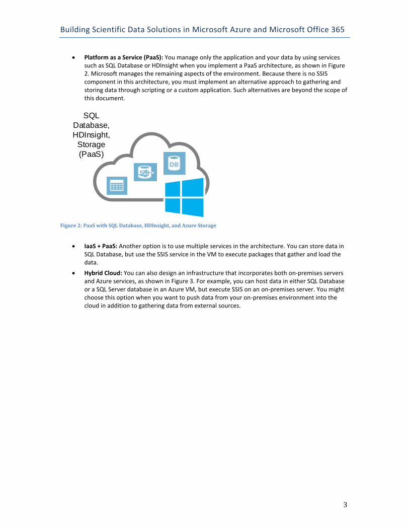
Platform as a Service (PaaS): You manage only the application and your data by using services such as SQL Database or HDInsight when you implement a PaaS architecture, as shown in Figure 2. Microsoft manages the remaining aspects of the environment. Because there is no SSIS component in this architecture, you must implement an alternative approach to gathering and storing data through scripting or a custom application. Such alternatives are beyond the scope of this document.

SQL

Database,

HDInsight,

Storage

(PaaS)

Figure 2: PaaS with SQL Database, HDInsight, and Azure Storage

IaaS + PaaS: Another option is to use multiple services in the architecture. You can store data in SQL Database, but use the SSIS service in the VM to execute packages that gather and load the data.

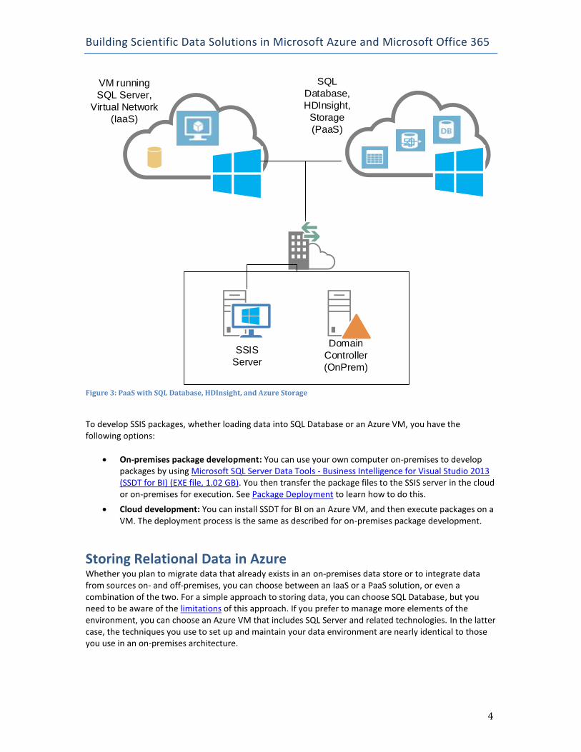
Hybrid Cloud: You can also design an infrastructure that incorporates both on-premises servers and Azure services, as shown in Figure 3. For example, you can host data in either SQL Database or a SQL Server database in an Azure VM, but execute SSIS on an on-premises server. You might choose this option when you want to push data from your on-premises environment into the cloud in addition to gathering data from external sources.

Building Scientific Data Solutions in Microsoft Azure and Microsoft Office 365

4

VM running

SQL Server,

Virtual Network

(IaaS)

SQL

Database,

HDInsight,

Storage

(PaaS)

Domain

Controller

(OnPrem)

SSIS

Server

Figure 3: PaaS with SQL Database, HDInsight, and Azure Storage

To develop SSIS packages, whether loading data into SQL Database or an Azure VM, you have the following options:

On-premises package development: You can use your own computer on-premises to develop packages by using Microsoft SQL Server Data Tools - Business Intelligence for Visual Studio 2013 (SSDT for BI) (EXE file, 1.02 GB). You then transfer the package files to the SSIS server in the cloud or on-premises for execution. See Package Deployment to learn how to do this.

Cloud development: You can install SSDT for BI on an Azure VM, and then execute packages on a VM. The deployment process is the same as described for on-premises package development.

Storing Relational Data in Azure Whether you plan to migrate data that already exists in an on-premises data store or to integrate data from sources on- and off-premises, you can choose between an IaaS or a PaaS solution, or even a combination of the two. For a simple approach to storing data, you can choose SQL Database, but you need to be aware of the limitations of this approach. If you prefer to manage more elements of the environment, you can choose an Azure VM that includes SQL Server and related technologies. In the latter case, the techniques you use to set up and maintain your data environment are nearly identical to those you use in an on-premises architecture.

Building Scientific Data Solutions in Microsoft Azure and Microsoft Office 365

5

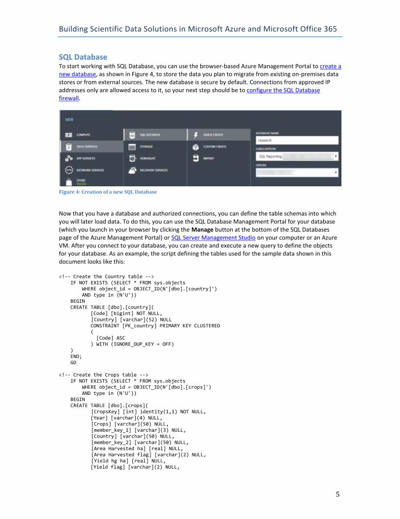
SQL Database To start working with SQL Database, you can use the browser-based Azure Management Portal to create a new database, as shown in Figure 4, to store the data you plan to migrate from existing on-premises data stores or from external sources. The new database is secure by default. Connections from approved IP addresses only are allowed access to it, so your next step should be to configure the SQL Database firewall.

Figure 4: Creation of a new SQL Database

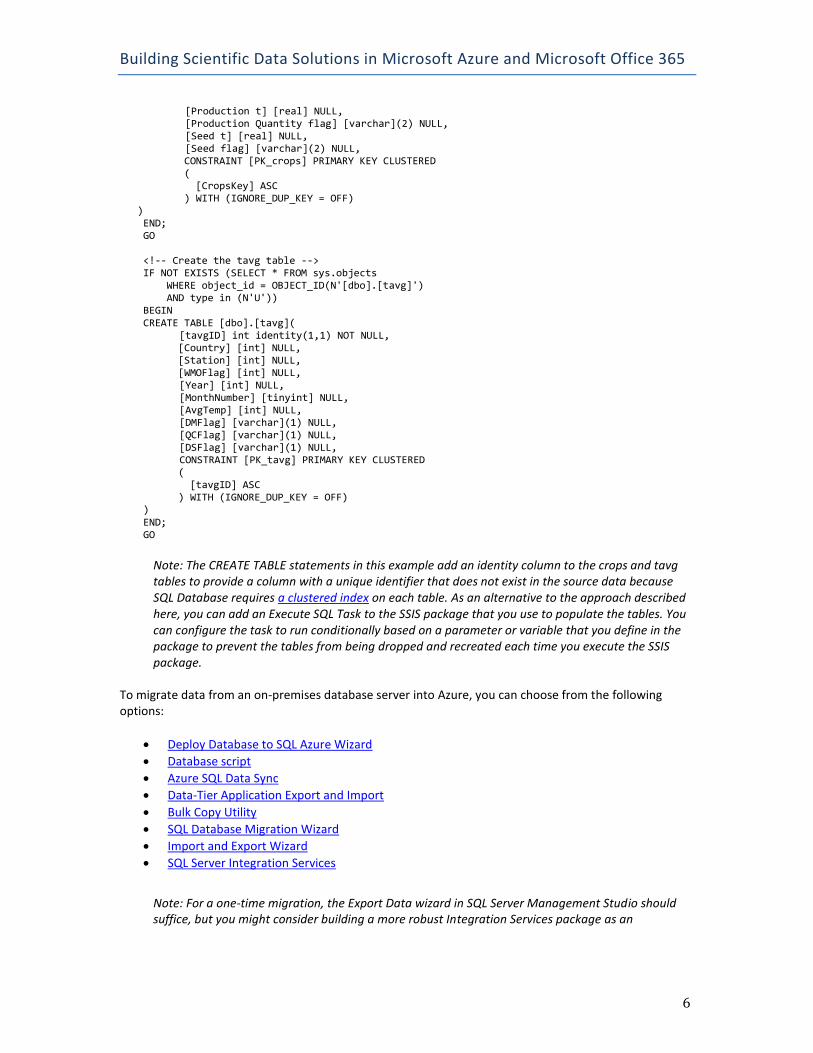
Now that you have a database and authorized connections, you can define the table schemas into which you will later load data. To do this, you can use the SQL Database Management Portal for your database (which you launch in your browser by clicking the Manage button at the bottom of the SQL Databases page of the Azure Management Portal) or SQL Server Management Studio on your computer or an Azure VM. After you connect to your database, you can create and execute a new query to define the objects for your database. As an example, the script defining the tables used for the sample data shown in this document looks like this: <!-- Create the Country table --> IF NOT EXISTS (SELECT * FROM sys.objects WHERE object_id = OBJECT_ID(N'[dbo].[country]') AND type in (N'U')) BEGIN CREATE TABLE [dbo].[country]( [Code] [bigint] NOT NULL, [Country] [varchar](52) NULL CONSTRAINT [PK_country] PRIMARY KEY CLUSTERED ( [Code] ASC ) WITH (IGNORE_DUP_KEY = OFF) ) END; GO <!-- Create the Crops table --> IF NOT EXISTS (SELECT * FROM sys.objects WHERE object_id = OBJECT_ID(N'[dbo].[crops]') AND type in (N'U')) BEGIN CREATE TABLE [dbo].[crops]( [CropsKey] [int] identity(1,1) NOT NULL, [Year] [varchar](4) NULL, [Crops] [varchar](50) NULL, [member_key_1] [varchar](3) NULL, [Country] [varchar](50) NULL, [member_key_2] [varchar](50) NULL, [Area Harvested ha] [real] NULL, [Area Harvested flag] [varchar](2) NULL, [Yield hg ha] [real] NULL, [Yield flag] [varchar](2) NULL,

Building Scientific Data Solutions in Microsoft Azure and Microsoft Office 365

6

[Production t] [real] NULL, [Production Quantity flag] [varchar](2) NULL, [Seed t] [real] NULL, [Seed flag] [varchar](2) NULL, CONSTRAINT [PK_crops] PRIMARY KEY CLUSTERED ( [CropsKey] ASC ) WITH (IGNORE_DUP_KEY = OFF) ) END; GO <!-- Create the tavg table --> IF NOT EXISTS (SELECT * FROM sys.objects WHERE object_id = OBJECT_ID(N'[dbo].[tavg]') AND type in (N'U')) BEGIN CREATE TABLE [dbo].[tavg]( [tavgID] int identity(1,1) NOT NULL, [Country] [int] NULL, [Station] [int] NULL, [WMOFlag] [int] NULL, [Year] [int] NULL, [MonthNumber] [tinyint] NULL, [AvgTemp] [int] NULL, [DMFlag] [varchar](1) NULL, [QCFlag] [varchar](1) NULL, [DSFlag] [varchar](1) NULL, CONSTRAINT [PK_tavg] PRIMARY KEY CLUSTERED ( [tavgID] ASC ) WITH (IGNORE_DUP_KEY = OFF) ) END; GO

Note: The CREATE TABLE statements in this example add an identity column to the crops and tavg tables to provide a column with a unique identifier that does not exist in the source data because SQL Database requires a clustered index on each table. As an alternative to the approach described here, you can add an Execute SQL Task to the SSIS package that you use to populate the tables. You can configure the task to run conditionally based on a parameter or variable that you define in the package to prevent the tables from being dropped and recreated each time you execute the SSIS package.

To migrate data from an on-premises database server into Azure, you can choose from the following options:

Deploy Database to SQL Azure Wizard

Database script

Azure SQL Data Sync

Data-Tier Application Export and Import

Bulk Copy Utility

SQL Database Migration Wizard

Import and Export Wizard

SQL Server Integration Services

Note: For a one-time migration, the Export Data wizard in SQL Server Management Studio should suffice, but you might consider building a more robust Integration Services package as an

Building Scientific Data Solutions in Microsoft Azure and Microsoft Office 365

7

alternative. In this package, you can separate the steps of copying schemas, adding clustered indexes, and copying data.

SQL Server in Azure VM Many of the options described in the previous section for moving data into a SQL Database are also useful for moving data into a SQL Server hosted in an Azure VM. In addition, you can also use the Deploy a SQL Server Database to a Windows Azure Virtual Machine wizard.

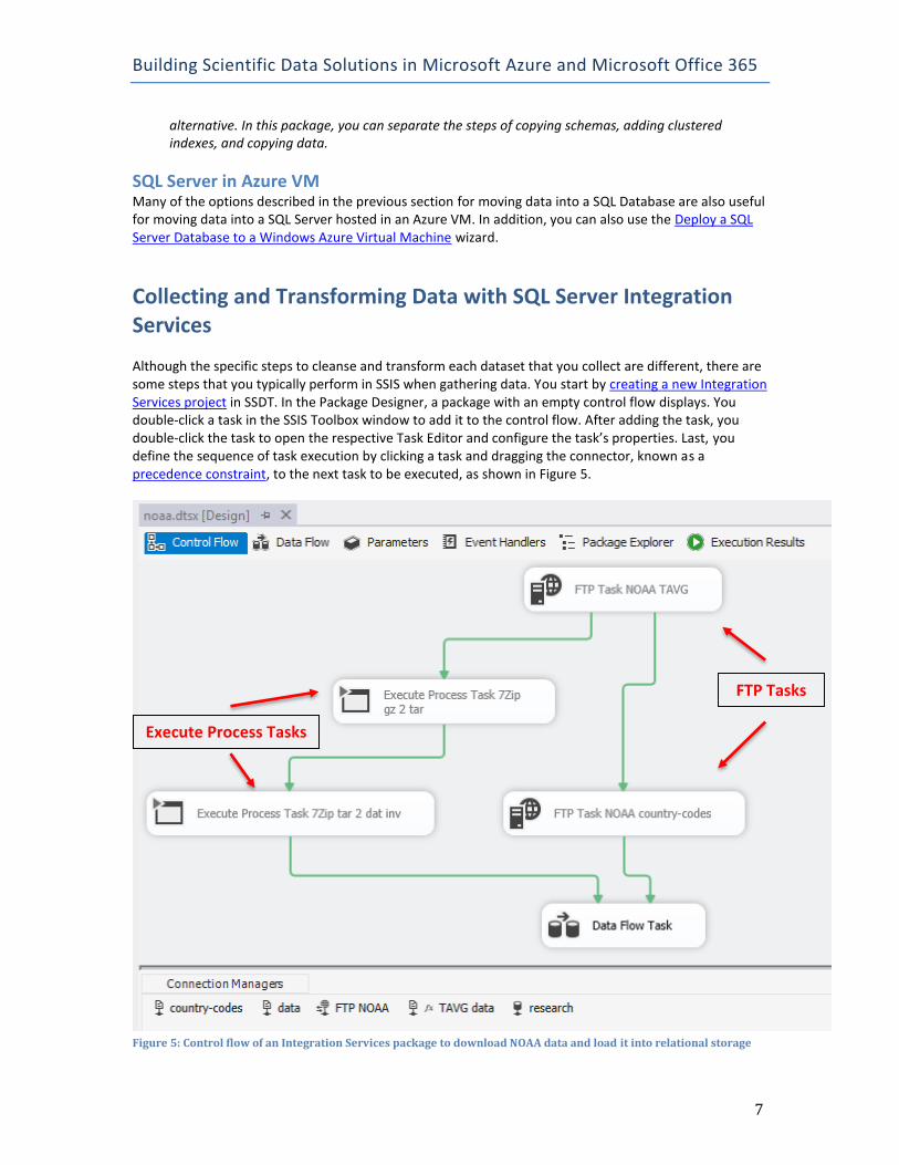
Collecting and Transforming Data with SQL Server Integration Services Although the specific steps to cleanse and transform each dataset that you collect are different, there are some steps that you typically perform in SSIS when gathering data. You start by creating a new Integration Services project in SSDT. In the Package Designer, a package with an empty control flow displays. You double-click a task in the SSIS Toolbox window to add it to the control flow. After adding the task, you double-click the task to open the respective Task Editor and configure the task’s properties. Last, you define the sequence of task execution by clicking a task and dragging the connector, known as a precedence constraint, to the next task to be executed, as shown in Figure 5.

Figure 5: Control flow of an Integration Services package to download NOAA data and load it into relational storage

FTP Tasks

Execute Process Tasks

Building Scientific Data Solutions in Microsoft Azure and Microsoft Office 365

8

In this example, there are several tasks in the control flow. FTP Task NOAA TAVG and FTP Task NOAA country-codes are FTP tasks that retrieve data from NOAA’s FTP server in separate steps. The Execute Process tasks, Execute Process Task 7Zip gz 2 tar and Execute Process Task 7Zip tar 2 dat inv, extract files from the compressed files that were downloaded. After all FTP tasks and Execute Process tasks have executed successfully, a Data Flow Task executes to connect to the extracted files, perform transformations to reshape the data, and load the data into a target database.

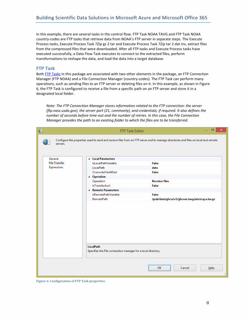
FTP Task Both FTP Tasks in this package are associated with two other elements in the package, an FTP Connection Manager (FTP NOAA) and a File Connection Manager (country-codes). The FTP Task can perform many operations, such as sending files to an FTP server or deleting files on it. In this example, as shown in Figure 6, the FTP Task is configured to receive a file from a specific path on an FTP server and store it in a designated local folder.

Note: The FTP Connection Manager stores information related to the FTP connection: the server (ftp.nass.usda.gov), the server port (21, commonly), and credentials, if required. It also defines the number of seconds before time-out and the number of retries. In this case, the File Connection Manager provides the path to an existing folder to which the files are to be transferred.

Figure 6: Configuration of FTP Task properties

Building Scientific Data Solutions in Microsoft Azure and Microsoft Office 365

9

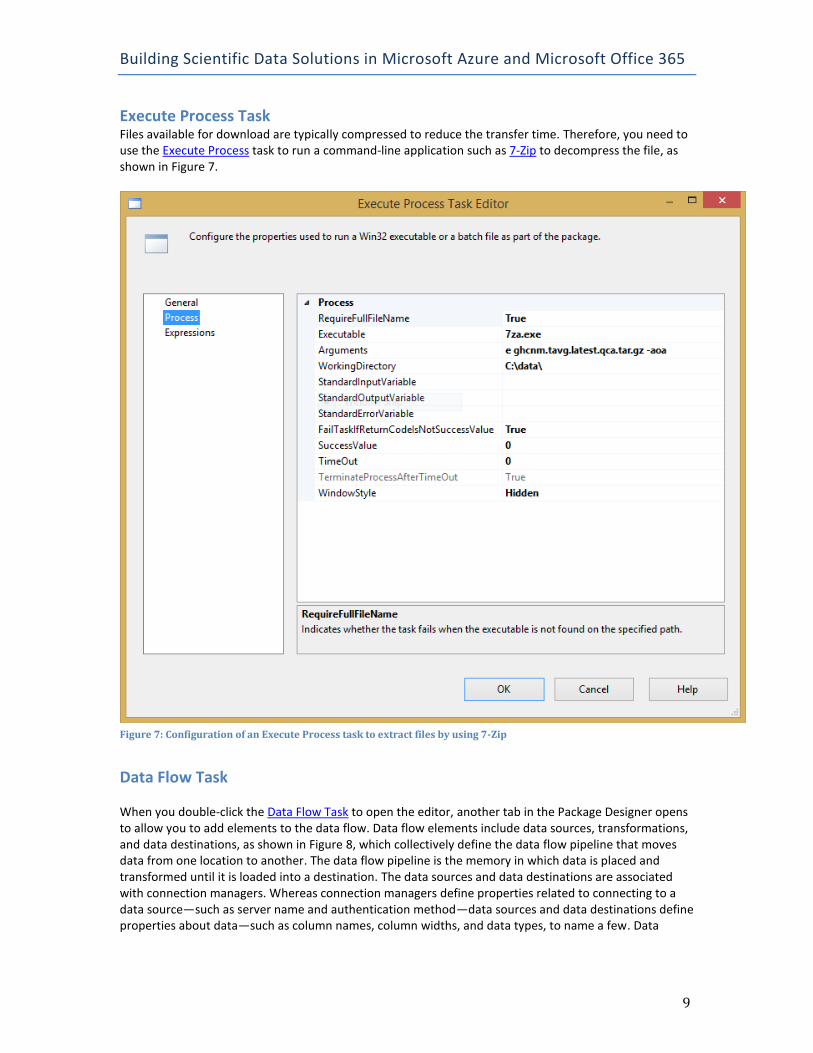
Execute Process Task Files available for download are typically compressed to reduce the transfer time. Therefore, you need to use the Execute Process task to run a command-line application such as 7-Zip to decompress the file, as shown in Figure 7.

Figure 7: Configuration of an Execute Process task to extract files by using 7-Zip

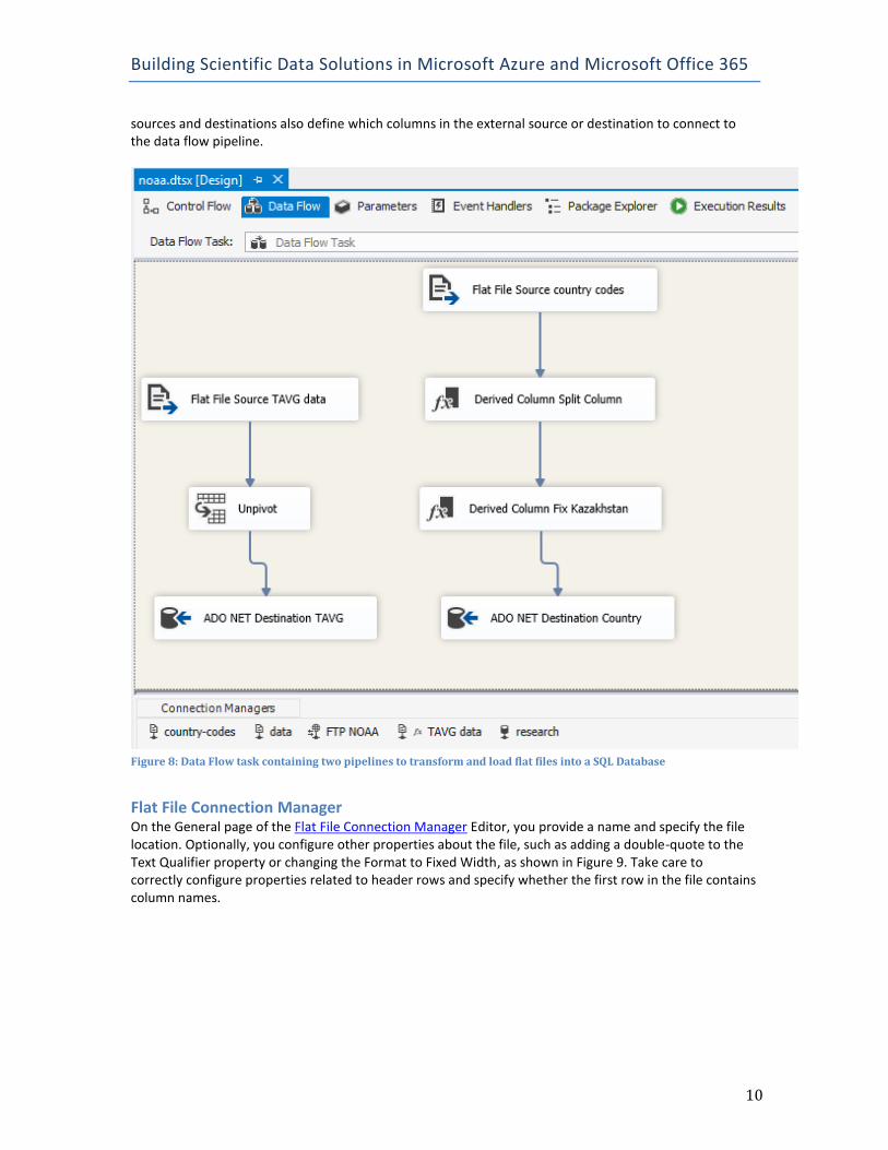
Data Flow Task When you double-click the Data Flow Task to open the editor, another tab in the Package Designer opens to allow you to add elements to the data flow. Data flow elements include data sources, transformations, and data destinations, as shown in Figure 8, which collectively define the data flow pipeline that moves data from one location to another. The data flow pipeline is the memory in which data is placed and transformed until it is loaded into a destination. The data sources and data destinations are associated with connection managers. Whereas connection managers define properties related to connecting to a data source—such as server name and authentication method—data sources and data destinations define properties about data—such as column names, column widths, and data types, to name a few. Data

Building Scientific Data Solutions in Microsoft Azure and Microsoft Office 365

10

sources and destinations also define which columns in the external source or destination to connect to the data flow pipeline.

Figure 8: Data Flow task containing two pipelines to transform and load flat files into a SQL Database

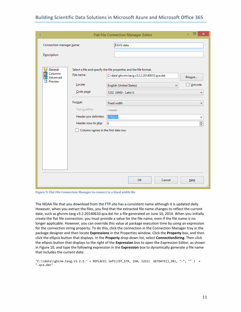
Flat File Connection Manager On the General page of the Flat File Connection Manager Editor, you provide a name and specify the file location. Optionally, you configure other properties about the file, such as adding a double-quote to the Text Qualifier property or changing the Format to Fixed Width, as shown in Figure 9. Take care to correctly configure properties related to header rows and specify whether the first row in the file contains column names.

Building Scientific Data Solutions in Microsoft Azure and Microsoft Office 365

11

Figure 9: Flat File Connection Manager to connect to a fixed width file

The NOAA file that you download from the FTP site has a consistent name although it is updated daily. However, when you extract the files, you find that the extracted file name changes to reflect the current date, such as ghcnm.tavg.v3.2.20140610.qca.dat for a file generated on June 10, 2014. When you initially create the flat file connection, you must provide a value for the file name, even if the file name is no longer applicable. However, you can override this value at package execution time by using an expression for the connection string property. To do this, click the connection in the Connection Manager tray in the package designer and then locate Expressions in the Properties window. Click the Property box, and then click the ellipsis button that displays. In the Property drop-down list, select ConnectionString. Then click the ellipsis button that displays to the right of the Expression box to open the Expression Editor, as shown in Figure 10, and type the following expression in the Expression box to dynamically generate a file name that includes the current date: "C:\\data\\ghcnm.tavg.v3.2.2." + REPLACE( left((DT_STR, 250, 1252) GETDATE(),10), "-", "" ) + ".qca.dat"

Building Scientific Data Solutions in Microsoft Azure and Microsoft Office 365

12

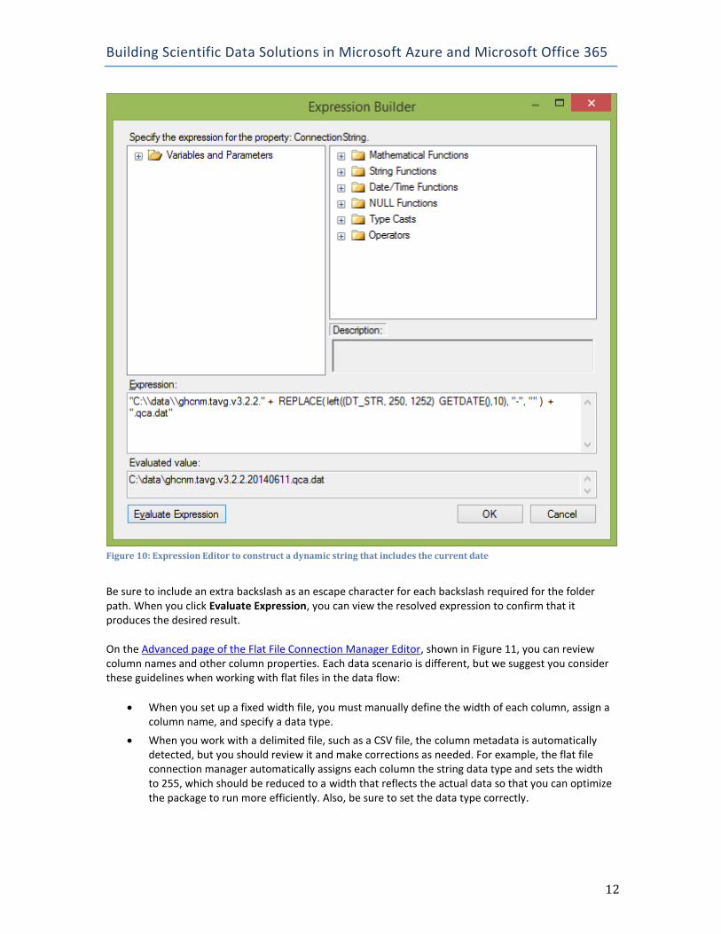
Figure 10: Expression Editor to construct a dynamic string that includes the current date

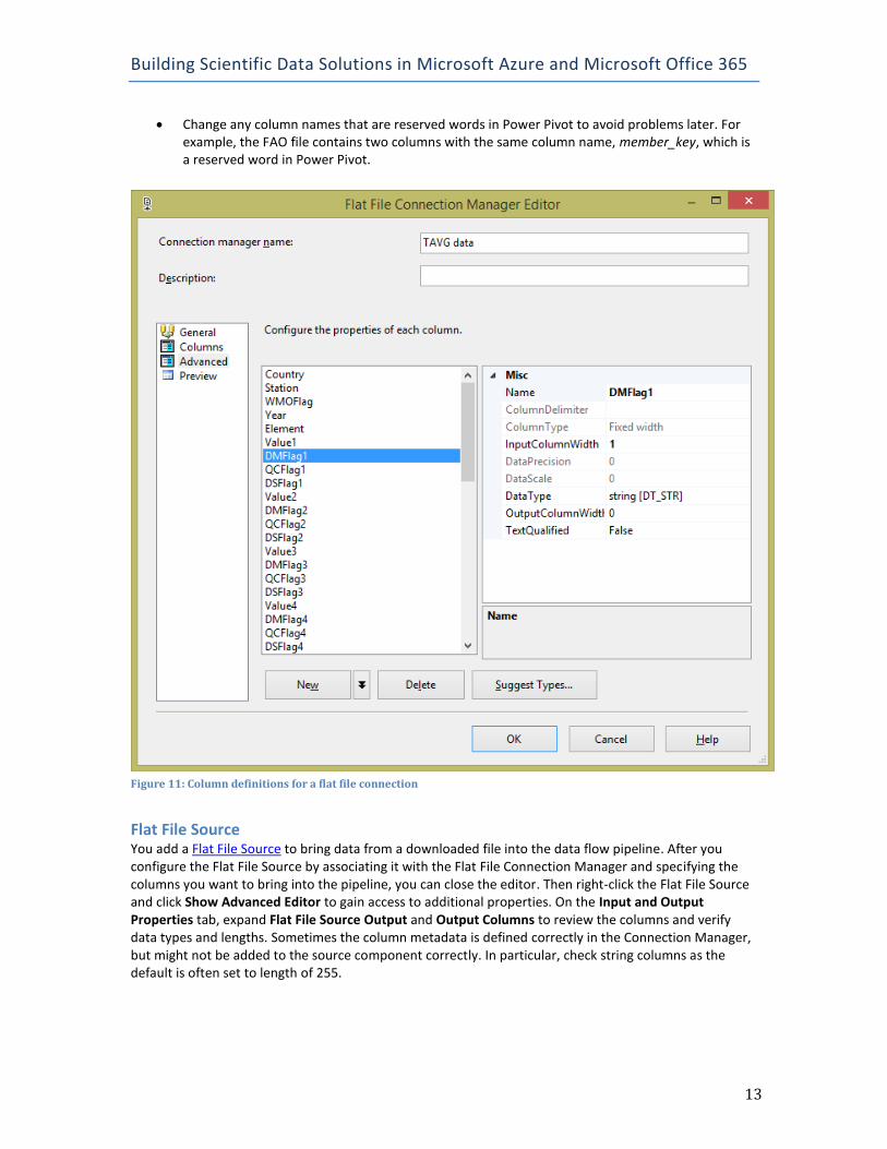
Be sure to include an extra backslash as an escape character for each backslash required for the folder path. When you click Evaluate Expression, you can view the resolved expression to confirm that it produces the desired result. On the Advanced page of the Flat File Connection Manager Editor, shown in Figure 11, you can review column names and other column properties. Each data scenario is different, but we suggest you consider these guidelines when working with flat files in the data flow:

When you set up a fixed width file, you must manually define the width of each column, assign a column name, and specify a data type.

When you work with a delimited file, such as a CSV file, the column metadata is automatically detected, but you should review it and make corrections as needed. For example, the flat file connection manager automatically assigns each column the string data type and sets the width to 255, which should be reduced to a width that reflects the actual data so that you can optimize the package to run more efficiently. Also, be sure to set the data type correctly.

Building Scientific Data Solutions in Microsoft Azure and Microsoft Office 365

13

Change any column names that are reserved words in Power Pivot to avoid problems later. For example, the FAO file contains two columns with the same column name, member_key, which is a reserved word in Power Pivot.

Figure 11: Column definitions for a flat file connection

Flat File Source You add a Flat File Source to bring data from a downloaded file into the data flow pipeline. After you configure the Flat File Source by associating it with the Flat File Connection Manager and specifying the columns you want to bring into the pipeline, you can close the editor. Then right-click the Flat File Source and click Show Advanced Editor to gain access to additional properties. On the Input and Output Properties tab, expand Flat File Source Output and Output Columns to review the columns and verify data types and lengths. Sometimes the column metadata is defined correctly in the Connection Manager, but might not be added to the source component correctly. In particular, check string columns as the default is often set to length of 255.

Building Scientific Data Solutions in Microsoft Azure and Microsoft Office 365

14

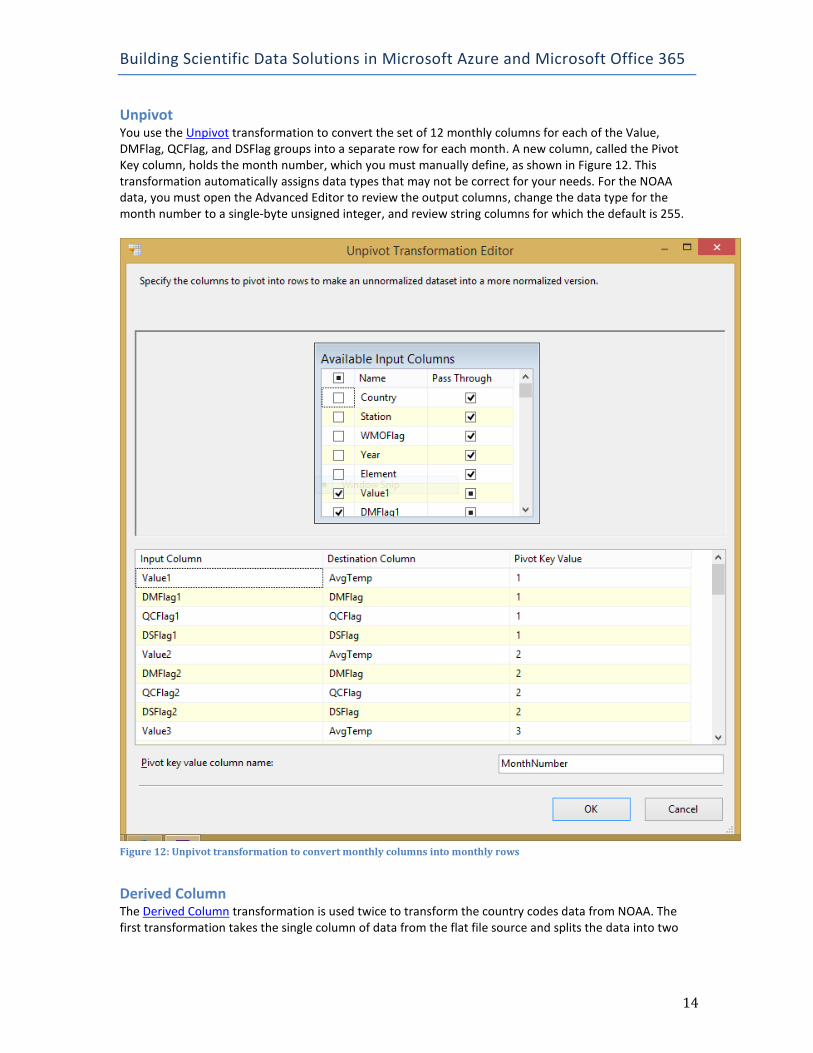
Unpivot You use the Unpivot transformation to convert the set of 12 monthly columns for each of the Value, DMFlag, QCFlag, and DSFlag groups into a separate row for each month. A new column, called the Pivot Key column, holds the month number, which you must manually define, as shown in Figure 12. This transformation automatically assigns data types that may not be correct for your needs. For the NOAA data, you must open the Advanced Editor to review the output columns, change the data type for the month number to a single-byte unsigned integer, and review string columns for which the default is 255.

Figure 12: Unpivot transformation to convert monthly columns into monthly rows

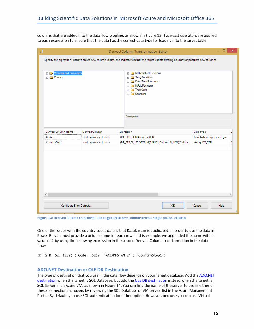
Derived Column The Derived Column transformation is used twice to transform the country codes data from NOAA. The first transformation takes the single column of data from the flat file source and splits the data into two

Building Scientific Data Solutions in Microsoft Azure and Microsoft Office 365

15

columns that are added into the data flow pipeline, as shown in Figure 13. Type cast operators are applied to each expression to ensure that the data has the correct data type for loading into the target table.

Figure 13: Derived Column transformation to generate new columns from a single-source column

One of the issues with the country codes data is that Kazakhstan is duplicated. In order to use the data in Power BI, you must provide a unique name for each row. In this example, we appended the name with a value of 2 by using the following expression in the second Derived Column transformation in the data flow: (DT_STR, 52, 1252) ([Code]==625? "KAZAKHSTAN 2" : [CountryStep1])

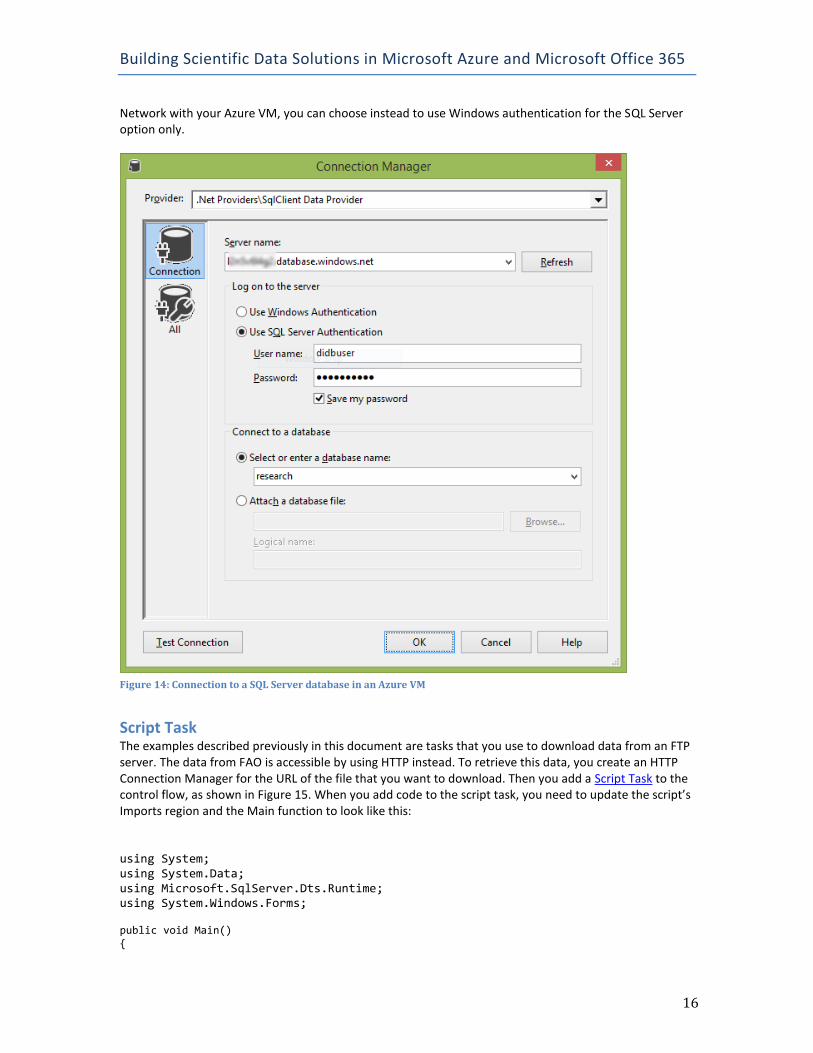
ADO.NET Destination or OLE DB Destination The type of destination that you use in the data flow depends on your target database. Add the ADO.NET destination when the target is SQL Database, but add the OLE DB destination instead when the target is SQL Server in an Azure VM, as shown in Figure 14. You can find the name of the server to use in either of these connection managers by reviewing the SQL Database or VM service list in the Azure Management Portal. By default, you use SQL authentication for either option. However, because you can use Virtual

Building Scientific Data Solutions in Microsoft Azure and Microsoft Office 365

16

Network with your Azure VM, you can choose instead to use Windows authentication for the SQL Server option only.

Figure 14: Connection to a SQL Server database in an Azure VM

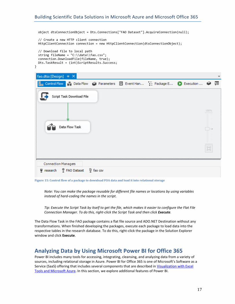
Script Task The examples described previously in this document are tasks that you use to download data from an FTP server. The data from FAO is accessible by using HTTP instead. To retrieve this data, you create an HTTP Connection Manager for the URL of the file that you want to download. Then you add a Script Task to the control flow, as shown in Figure 15. When you add code to the script task, you need to update the script’s Imports region and the Main function to look like this: using System; using System.Data; using Microsoft.SqlServer.Dts.Runtime; using System.Windows.Forms; public void Main() {

Building Scientific Data Solutions in Microsoft Azure and Microsoft Office 365

17

object dtsConnectionObject = Dts.Connections["FAO Dataset"].AcquireConnection(null); // Create a new HTTP client connection HttpClientConnection connection = new HttpClientConnection(dtsConnectionObject); // Download file to local path string fileName = "C:\\data\\fao.csv"; connection.DownloadFile(fileName, true); Dts.TaskResult = (int)ScriptResults.Success; }

Figure 15: Control flow of a package to download FOA data and load it into relational storage

Note: You can make the package reusable for different file names or locations by using variables instead of hard-coding the names in the script.

Tip: Execute the Script Task by itself to get the file, which makes it easier to configure the Flat File Connection Manager. To do this, right-click the Script Task and then click Execute.

The Data Flow Task in the FAO package contains a flat file source and ADO.NET Destination without any transformations. When finished developing the packages, execute each package to load data into the respective tables in the research database. To do this, right-click the package in the Solution Explorer window and click Execute.

Analyzing Data by Using Microsoft Power BI for Office 365 Power BI includes many tools for accessing, integrating, cleansing, and analyzing data from a variety of sources, including relational storage in Azure. Power BI for Office 365 is one of Microsoft’s Software as a Service (SaaS) offering that includes several components that are described in Visualization with Excel Tools and Microsoft Azure. In this section, we explore additional features of Power BI.

Building Scientific Data Solutions in Microsoft Azure and Microsoft Office 365

18

Creating a Power Pivot Model Power Pivot is a built-in add-in for Microsoft Excel 2013 (and available as a downloadable add-in for Excel 2010) that you use to store, model, and analyze large volumes of data. With Power Pivot, you can work with more data than an Excel workbook supports because it uses the same xVelocity in-memory columnar technology that SQL Server and Analysis Services use to compress data and optimize query executions. To get started, you can pull data from the relational storage in Azure into the Power Pivot model. However, rather than retrieve every row of data, you can apply filters to focus on a particular date range, such as 2001 to 2005 as shown in the subsequent examples, or to remove records with missing data, such as indicated by the -9999 value in the AvgTemp column of the NOAA data. In Power Pivot, you first open the Power Pivot interface by clicking the Manage button on the Power Pivot tab of the ribbon, and then go to the Get External Data section of the Power Pivot tab of the ribbon, and then choose one of the following options:

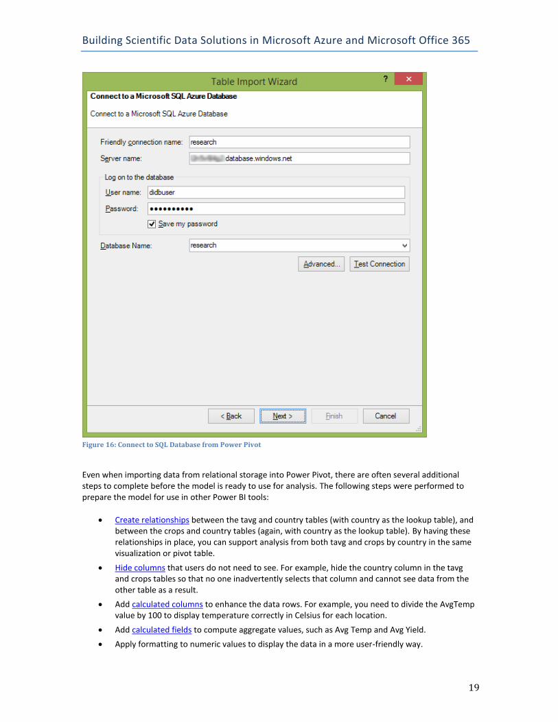
For SQL Database, click From Other Sources and then Microsoft SQL Azure. When you click Next, you provide the fully qualified server name (as shown in Figure 16), login credentials, and the name of the database.

For SQL Server in an Azure VM, click From Database and then From SQL Server. Type the name of the VM server and provide the SQL login.

Building Scientific Data Solutions in Microsoft Azure and Microsoft Office 365

19

Figure 16: Connect to SQL Database from Power Pivot

Even when importing data from relational storage into Power Pivot, there are often several additional steps to complete before the model is ready to use for analysis. The following steps were performed to prepare the model for use in other Power BI tools:

Create relationships between the tavg and country tables (with country as the lookup table), and between the crops and country tables (again, with country as the lookup table). By having these relationships in place, you can support analysis from both tavg and crops by country in the same visualization or pivot table.

Hide columns that users do not need to see. For example, hide the country column in the tavg and crops tables so that no one inadvertently selects that column and cannot see data from the other table as a result.

Add calculated columns to enhance the data rows. For example, you need to divide the AvgTemp value by 100 to display temperature correctly in Celsius for each location.

Add calculated fields to compute aggregate values, such as Avg Temp and Avg Yield.

Apply formatting to numeric values to display the data in a more user-friendly way.

Building Scientific Data Solutions in Microsoft Azure and Microsoft Office 365

20

Add a date dimension from Azure Marketplace (by author Boyan Penev), create a calculated column in tavg and in crops to generate a date key that you can use for relationships, and then create relationships between the date dimension and crops and between dates and tavg. The calculated column for the date looks like this:

=date([Year],right("00"&[MonthNumber],2),"01

Add a calculated column to the dates table to use in forecasting:

=Year & MonthOfYear

Click the MonthInCalendar column, then click Sort By Column to sort this data by the calculated column created in the previous step.

Select the YearKey column in the date dimension. Then, on the Advanced tab of the ribbon, click Summarize By, and then click Do Not Summarize to prevent this column from included in the calculations of values.

On the Design tab, with dates open as the current table, click Mark As Date Table to configure Excel to work with this table as dates.

Add a calculated column to the tavg table, set a Date data type on the column, and then use the following expression to create date column for use in forecasting in Power BI for Office 365: =date([Year],[MonthNumber],"01")

Visualizing Data in Power View After you have a Power Pivot data model prepared, you can insert a Power View report into the workbook. A Power View report can display multiple styles of visualizations, as shown in Figure 17. By combining different types of data sets in a single Power Pivot model and then using visualizations to filter and explore the model, you can discover any relationships that might exist between the data sources in scatter plots that display changes in the data over time with a play axis, or line charts that compare data categories over time. Furthermore, you can click an item such as a line or a legend element in one chart. Power View then applies a cross-filter, also known as highlighting, to other charts in the same report, allowing you to assess the selected item’s contribution to the overall measurement. You can also apply separate filters to the report, either to all items in the same report (by adding fields to the Filters/View pane) or to separate filters for each item. In Figure 17, the entire view is filtered to show data related to Belgium. The view includes three line charts to illustrate the average yield of various crops across multiple years, the average temperature for the same years, and the average monthly temperature by year. In the top left of the view, a scatter chart displays one bubble for each year to visualize the change in average production relative to average temperature by year. A play axis below the chart animates the scatter chart to display one bubble at a time, or you can view the historical trajectory of the bubbles by clicking one of them in the chart.

Building Scientific Data Solutions in Microsoft Azure and Microsoft Office 365

21

Figure 17: A Power View report containing four interactive and interconnected data visualizations

Publishing to Office 365 If you are signed into an Office 365 account, you can save your workbook to a Power BI site in the SharePoint Online library for others in your organization to view. You can also upload a document directly to the library. Either way, your next step is to enable the workbook for Power BI. You can also selectively add workbooks to use with Power BI Questions & Answers (Q&A). Another option for published workbooks is to schedule a daily or weekly data refresh as long as the data source is one that is supported. At the time of this writing, supported data sources include:

SQL Server

SQL Database

OData feeds, including SharePoint lists and Azure Marketplace, among others

On-premises data sources with a data management gateway connection

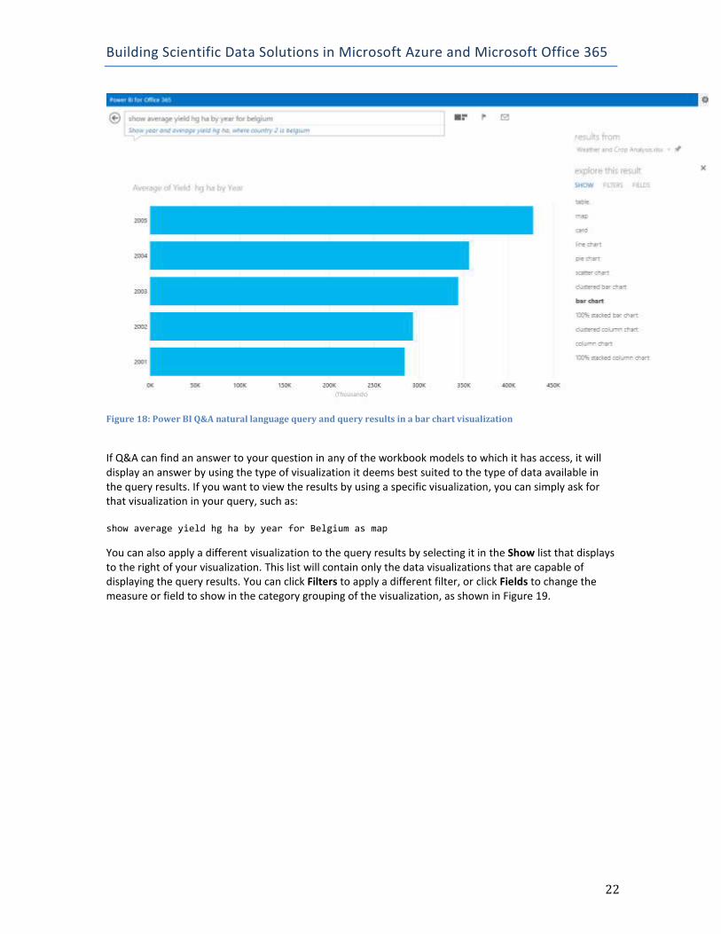
Querying the Data by using Power BI Q&A Power BI Q&A allows you to ask question of your data using natural language questions rather than by using the query language syntax typically associated with ad hoc reporting. If you have workbooks added to Q&A, you can click Ask With Power BI Q&A in the top right corner of screen from the Power BI site. Then, start typing a question in the Q&A question box (shown in Figure 18), such as: show average yield hg ha by year for Belgium

Building Scientific Data Solutions in Microsoft Azure and Microsoft Office 365

22

Figure 18: Power BI Q&A natural language query and query results in a bar chart visualization

If Q&A can find an answer to your question in any of the workbook models to which it has access, it will display an answer by using the type of visualization it deems best suited to the type of data available in the query results. If you want to view the results by using a specific visualization, you can simply ask for that visualization in your query, such as: show average yield hg ha by year for Belgium as map

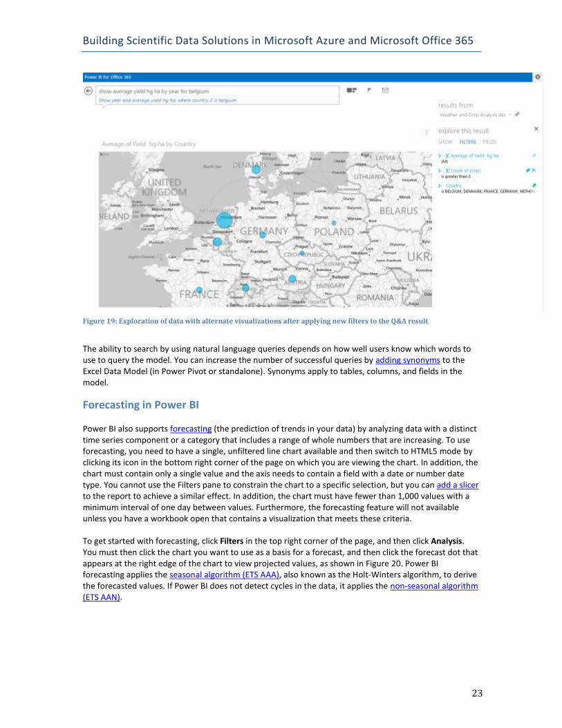
You can also apply a different visualization to the query results by selecting it in the Show list that displays to the right of your visualization. This list will contain only the data visualizations that are capable of displaying the query results. You can click Filters to apply a different filter, or click Fields to change the measure or field to show in the category grouping of the visualization, as shown in Figure 19.

Building Scientific Data Solutions in Microsoft Azure and Microsoft Office 365

23

Figure 19: Exploration of data with alternate visualizations after applying new filters to the Q&A result

The ability to search by using natural language queries depends on how well users know which words to use to query the model. You can increase the number of successful queries by adding synonyms to the Excel Data Model (in Power Pivot or standalone). Synonyms apply to tables, columns, and fields in the model.

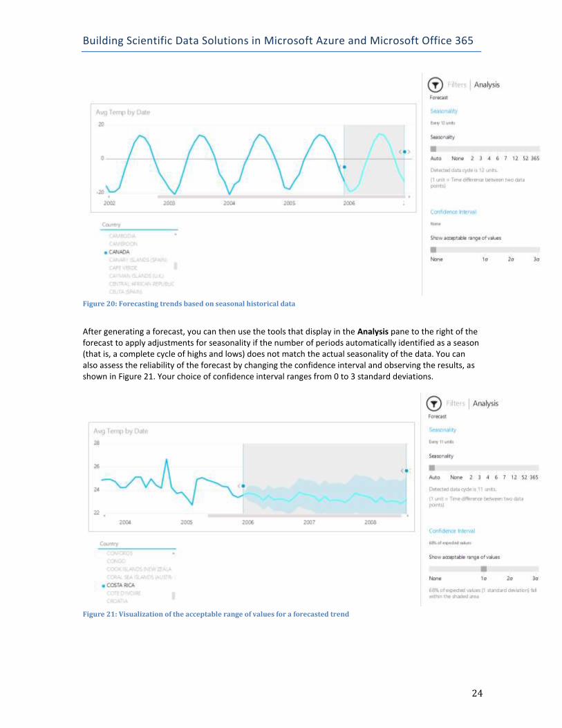
Forecasting in Power BI Power BI also supports forecasting (the prediction of trends in your data) by analyzing data with a distinct time series component or a category that includes a range of whole numbers that are increasing. To use forecasting, you need to have a single, unfiltered line chart available and then switch to HTML5 mode by clicking its icon in the bottom right corner of the page on which you are viewing the chart. In addition, the chart must contain only a single value and the axis needs to contain a field with a date or number date type. You cannot use the Filters pane to constrain the chart to a specific selection, but you can add a slicer to the report to achieve a similar effect. In addition, the chart must have fewer than 1,000 values with a minimum interval of one day between values. Furthermore, the forecasting feature will not available unless you have a workbook open that contains a visualization that meets these criteria. To get started with forecasting, click Filters in the top right corner of the page, and then click Analysis. You must then click the chart you want to use as a basis for a forecast, and then click the forecast dot that appears at the right edge of the chart to view projected values, as shown in Figure 20. Power BI forecasting applies the seasonal algorithm (ETS AAA), also known as the Holt-Winters algorithm, to derive the forecasted values. If Power BI does not detect cycles in the data, it applies the non-seasonal algorithm (ETS AAN).

Building Scientific Data Solutions in Microsoft Azure and Microsoft Office 365

24

Figure 20: Forecasting trends based on seasonal historical data

After generating a forecast, you can then use the tools that display in the Analysis pane to the right of the forecast to apply adjustments for seasonality if the number of periods automatically identified as a season (that is, a complete cycle of highs and lows) does not match the actual seasonality of the data. You can also assess the reliability of the forecast by changing the confidence interval and observing the results, as shown in Figure 21. Your choice of confidence interval ranges from 0 to 3 standard deviations.

Figure 21: Visualization of the acceptable range of values for a forecasted trend

Building Scientific Data Solutions in Microsoft Azure and Microsoft Office 365

25

Summary Microsoft Azure and Office 365 expand your options for scientific data analysis in the cloud, whether you choose to implement an IaaS or PaaS architecture or a hybrid architecture bridging the cloud and your on-premises resources. Azure and Office 365 enable you to focus on working with your data without the overhead of building and managing the necessary technical infrastructure. Simply provision a storage service, by using either SQL Database or an Azure VM hosting SQL Server, and then migrate your data into that storage by using a tool like SSIS. With the data cleansed and transformed, you can explore it with Power BI to discover correlations or assess data trends with forecasting tools, helping you uncover fresh insights.

© 2014 Microsoft Corporation. All rights reserved. Except where otherwise noted, content on this site is licensed under a Creative Commons Attribution-NonCommercial 3.0 License.