CARNEGIE ~ MELLONDepartment of Electrical and Computer Engineering~

Bulk Coupled Stability Analysis

of a

Finite Conducting Fluid Layer

in a

Tangentially Incident

Alternating Magnetic Field

Bulk Coupled Stability Analysis

of a

Finite Conducting Fluid Layer

in a

Tangentially Incident

Alternating Magnetic Field

A Thesis

Submitted to the Graduate School

In Partial Fulfillment of the Requirements

for the degree of

Master of Science

in

Electrical and Computer Engineering

by

Charles H. Winstead

Camegie Mellon University

Pittsburgh, PA

10 May 1991

Contents

1.0 Introduction

2.0

3.0

Derivation of Governing Equations

2.1 Equilibrium

2.2 Perturbation

2.3 Limiting Cases

Method of Solution

4

5

9

18

20

4.0 Results

4.1

4.2

4.3

4.4

Experimental Parameter Values

Solution of Benard Instability

Solution of the Electromechanical Model

Results of the Electrothermal Model

24

24

25

26

30

5.0 Conclusions 39

i

List of Figures

Figure 1:

Figure 2:

Figure 3:

Figure 4:

Figure 5:

Figure 6:

Figure 7:

Figure 8:

Figure 9:

Figure 10:

Figure 11:

Figure 12:

Figure 13:

Figure 14:

Figure 15:

Figure 16:

Figure 17:

Figure 18:

Figure 19:

Figure 20:

Fluid Layer Geometry in Equilibrium.

The Three Sets of Boundaries.

M vs ~ for Perfectly Conducting Boundaries, no Thermal Coupling.

~ vs ~ for Perfectly Conducting Boundaries, no Thermal Coupling.

M vs ~ for Mixed Boundaries, no Thermal Coupling.

~ vs ~ for Mixed Boundaries, no Thermal Coupling.

Equilibrium Temperature Profile for Perfectly Conducting Boundaries.

M vs ~ for a Thermally Coupled Fluid Layer bounded by Conductors.

Equilibrium Temperature Profile for the Inverted Mixed Boundaries.

M vs ~ for a Thermally Coupled Fluid Layer with Inverted Mixed Boundaries.

Equilibrium Temperature Profile for Modified Convection in Mixed Boundaries.

M vs ~ for both models using Mixed Boundaries and Modified Convection.

Growth Rates for the Electromechanical Model with Mixed Boundary Conditions.

Growth Rates for the Electrothermal Modal with Mixed Boundaries and

Modified Convection.

Velocity Stream Lines for Electromechanical Instability.

Velocity Stream Lines for Electrothermal Instability.

Magnetic Field Lines for Electromechanical Instability.

Magnetic Field Lines for Electrothermal Instability.

Lines of Constant Temperature for Electromechanical Instability.

Lines of Constant Temperature for Electrothermal Instability.

2

6

28

28

29

29

30

31

32

28

33

34

35

35

36

36

37

37

38

38

ii

Bulk Coupled Stability Analysis of a Conducting Fluid Layer

in a Tangentially Incident Alternating Magnetic Field

Abstract

A liquid metal layer under the influence of a tangentially incident altemating magnetic

field is known to pass from a region of bulk coupled stability to a region of bulk coupled

instability. A model of the instability based on electromechanical coupling accurately

predicts the magnitude of the applied magnetic field required to produce instability, but

predicts growth rates which are orders of magnitude slower than experimentally observed.

In the model developed here, thermal effects due to the ohmic heating that results from

induced eddy currents are added to the electromechanical model. A linearized stability

model is developed and reduces to a linear system of ordinary differential equations with

non-constant coefficients. A technique for solving these equations based on a fourth-order

Runge-Kutta method is implemented. The results of this analysis are then compared to

the previous results based upon a model without thermal effects. The model including

thermal effects predicts growth rates closer to observed values, but significantly alters the

predicted field magnitude necessary to initiate instability.

1.0 Introduction

A high frequency magnetic field incident upon a conducting medium induces eddy currents and creates

Lorentz forces. These forces have been used in both the shaping and mixing of liquid metals. Asai has

discussed the advantages of using magnetic forces for material processing.[1] Fugate has developed a

method capable of both predicting the shape of a levitated liquid metal given a distribution of source

currents, and prescribing the distribution of currents that will create a desired shape.[2] Fugate’s

development of the free movement method, which determines the shape of a conducting liquid under

magnetic forces, assumes that the conductivity is large enough to confine the induced currents to the

surface of the metal.

The problem considered in this analysis is the behavior of a liquid metal of finite conductivity under

the influence of a high frequency magnetic field. A magnetic field of angular frequency to tangentially

incident upon a metal with electrical conductivity ~ and permittivity p. will diffuse into the metal with a

skin depth defined by ~5 --- (2/to~tcr)~. The effects of the magnetic field on a motionless liquid will reach

approximately one or two skin depths into the metal, which for most liquid metals is on the order of

millimeters for a field applied at a frequency in the kHz range. The fact that the field is contained within

such a small distance prompted Fugate and others to model the effects as purely constrained to the surface.

However, when the liquid undergoes internal motion, the effects of the applied magnetic field penetrate

several skin depths into the metal. In addition, fluid motion could have significant effects in applications

involving the containment of cooling liquid metal, despite the fact that the motion is confined to within

few skin depths from the-surface. These phenomena of finite conducting systems justify an in-depth

study of the effect of an applied field on a finite conducting liquid metal.

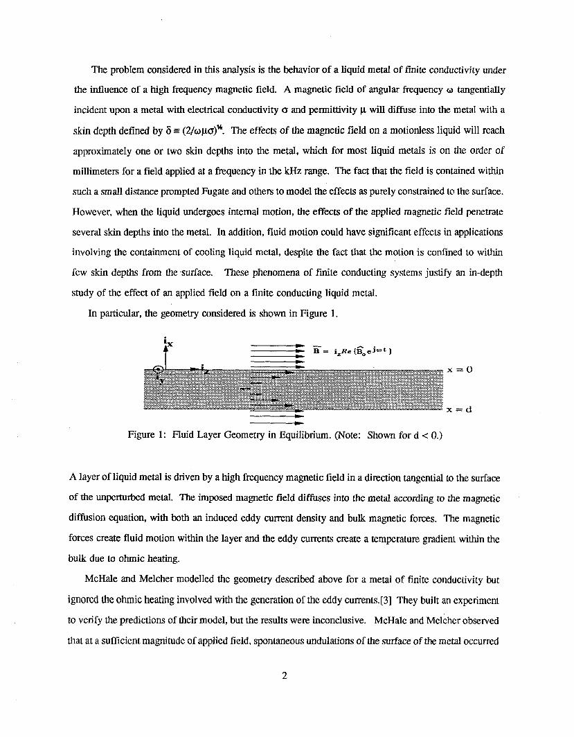
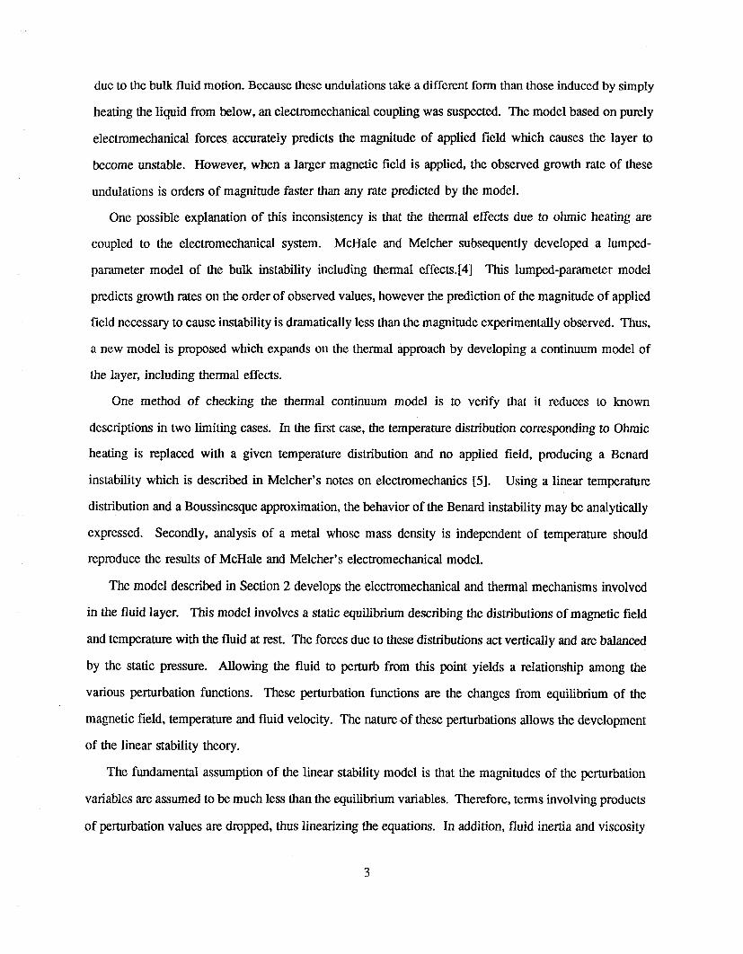
In particular, the geometry considered is shown in Figure 1.

Figure I: Fluid Layer Geometry in Equilbrium. (Note: llown for d ~ 0.)

x=O

x=d

A layer of liquid metal is driven by a high frequency magnetic field in a direction tangential to the surface

of the unperturbed metal. The imposed magnetic field diffuses into the metal according to the magnetic

diffusion equation, with beth an induced eddy current density and bulk magnetic forces. The magnetic

forces create fluid motion within the layer and the eddy currents create a temperature gradient within the

bulk due to ohmic heating.

McHale and Melcher modelled the geometry described above for a metal of finite conductivity but

ignored the ohmic heating involved with the generation of the eddy currents. [3] They built an experiment

to verify the predictions of their model, but the results were inconclusive. McHale and Melcher observed

that at a sufficient magnitude of applied field, spontaneous undulations of the surface of the metal occurred

2

due to the bulk fluid motion. Because these undulations take a different form than those induced by simply

heating the liquid from below, an electromechanical coupling was suspected. The model based on purely

electromechanical forces accurately predicts the magnitude of applied field which causes the layer to

become unstable. However, when a larger magnetic field is applied, the observed growth rate of these

undulations is orders of magnitude faster than any rate predicted by the model.

One possible explanation of this inconsistency is that the thermal effects due to ohmic heating are

coupled to the electromechanical system. McHale and Melcher subsequently developed a lumped-

parameter model of the bulk instability including thermal effects.[4] This lumped-parameter model

predicts growth rates on the order of observed values, however the prediction of the magnitude of applied

field necessary to cause instability is dramatically less than the magnitude experimentally observed. Thus,

a new model is proposed which expands on the thermal approach by developing a continuum model of

the layer, including thermal effects.

One method of checking the thermal continuum model is to verify that it reduces to known

descriptions in two limiting cases. In the first case, the temperature distribution corresponding to Ohmic

heating is replaced with a given temperature distribution and no applied fidd, producing a Benard

instability which is described in Melcher’s notes on electromechanics [5]. Using a linear temperature

distribution and a Boussinesque approximation, the behavior of the Benard instability may be analytically

expressed. Secondly, analysis of a metal whose mass density is independent of temperature should

reproduce the results of McHale and Melcher’s electromechanical model.

The model described in Section 2 develops the electromechanical and thermal mechanisms involved

in the fluid layer. This model involves a static equilibrium describing the distributions of magnetic field

and temperature with the fluid at rest. The forces due to these distributions act vertically and are balanced

by the static pressure. Allowing the fluid to perturb from this point yields a relationship among the

various perturbation functions. These perturbation functions are the changes from equilibrium of the

magnetic field, temperature and fluid velocity. The nature .of these perturbations allows the development

of the linear stability theory.

The fundamental assumption of the linear stability model is that the magnitudes of the perturbation

variables are assumed to be much less than the equilibrium variables. Therefore, terms involving products

of perturbation values are dropped, thus linearizing the equations. In addition, fluid inertia and viscosity

3

tend to dampen motions that occur at twice the frequency of the applied field, resulting in a ’time-

averaging’ property that justifies neglecting terms in the fluid motion equations that vary at twice the

frequency of the applied field. Finally, a form for the fluid velocity is used that assumes the variation in

the y and z directions is sinusoidal, prompted by the infinite nature of the geometry and the constant

equilibrium structure in these directions.

The result of the linear stability model is a linear set of ordinary non-constant coefficient complex

differential equations that are constrained by the boundary conditions imposed at the two surfaces x=0,

and x=d. A fourth order Runge-Kutta method is used to determine the coefficients in the linear

relationship between the functions and their derivatives evaluated at one surface and the functions and their

derivatives evaluated at the other surface. This relationship satisfies the given boundary conditions while

allowing internal fluid motion only for discrete combinations of applied field, growth rate, and wave

number. The result is a set of growth rate eigenvalues for any specified wave number and applied field,

or said another way, at a specified field, this results in the dispersion relation between growth rate and

wave number for each instability mode.

The organization of the development of the thermal continuum model follows. Section 2 details the

derivation of the governing equations; Section 2.1 describes equilibrium and Section 2.2 develops the

perturbation equations. Once a set of coupled equations are derived, Section 2.3 discusses the limiting

cases used to verify the model. Section 3 describes a method of solving these equations, results of which

are summarized in Section 4. Conclusions based on these results are presented in Section 5.

2.0 Derivation of Governing Equations

The equations that describe the behavior of a layer of liquid metal with finite conductivity driven by

a tangentially incident magnetic field are inherently non-linear. The method employed to solve them is

broken down into two steps. In the first step, a simple equilibrium structure is chosen, about which the

equations are linear and can be analytically solved. The behavior of the fluid is then allowed to deviate

from equilibrium, and the resulting non-linear equations govern the changes, or perturbations, from the

equilibrium. However, the magnitudes of these perturbations are assumed to be much less than those in

equilibrium. Therefore, the non-linear terms in the perturbation equations are neglected, and the resulting

equations analyzed using the properties of linear systems. While this approach is not exact, the hope is

4

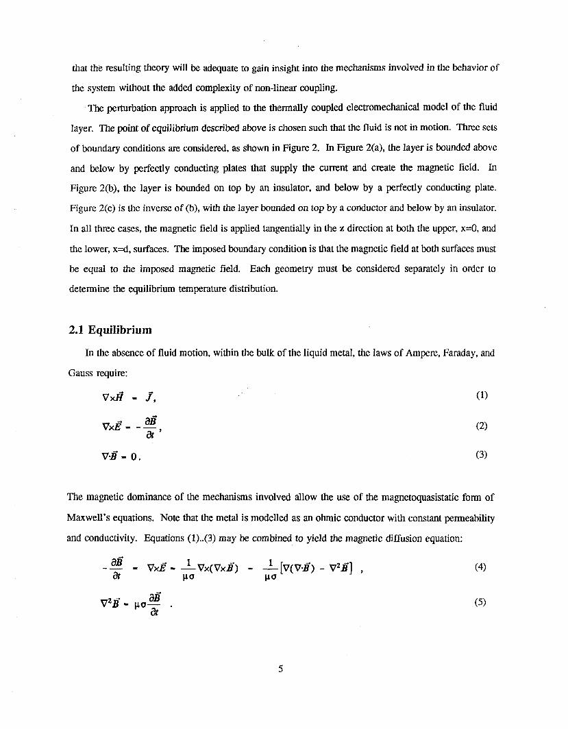
that the resulting theory will be adequate to gain insight into the mechanisms involved in the behavior of

the system without the added complexity of non-linear coupling.

The perturbation approach is applied to the thermally coupled electromechanical model of the fluid

layer. The point of equilibrium described above is chosen such that the fluid is not in motion. Three sets

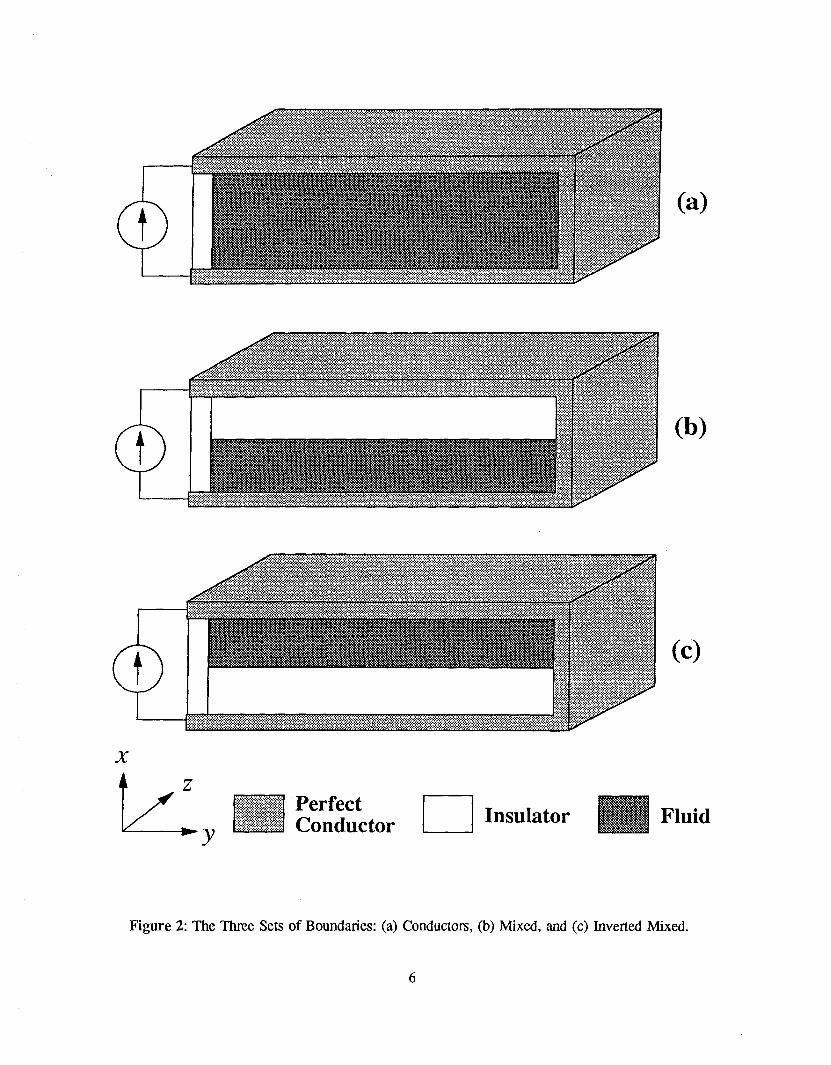
of boundary conditions are considered, as shown in Figure 2. In Figure 2(a), the layer is bounded above

and below by perfectly conducting plates that supply the current and create the magnetic field. In

Figure 2(b), the layer is bounded on top by an insulator, and below by a perfectly conducting plate.

Figure 2(c) is the inverse of (b), with the layer bounded on top by a conductor and below by an insulator.

In all three cases, the magnetic field is applied tangentially in the z direction at both the upper, x=0, and

the lower, x=d, surfaces. The imposed boundary condition is that the magnetic field at both surfaces must

be equal to the imposed magnetic field. Each geometry must be considered separately in order to

determine the equilibrium temperature distribution.

2.1 Equilibrium

In the absence of fluid motion, within the bulk of the liquid metal, the laws of Ampere, Faraday, and

Gauss require:

= j, " (1)

v×~ a# (2)at’

v.#- o. (3)

The magnetic dominance of the mechanisms involved allow the use of the magnetoquasistatic form of

Maxwell’s equations. Note that the metal is modelled as an ohmic conductor with comma-at permeability

and conductivity. Equations (1)..(3) may be combined to yield the magnetic diffusion equation:

V×/~ -- ~ Vx(Vx#) - _~1 [V(V./~) - V2~] (4)I.tO

(a)

(b)

(c)

.X

~z ~PerfectConductor ~Insulat°r WFluid~y

Figure 2: The Three Sets of Boundaries: (a) Conductors, 0a) Mixed, and (c) Inverted Mixed.

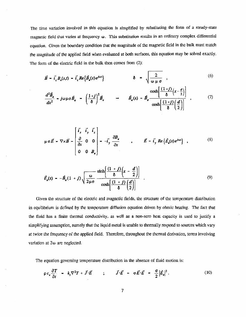
The time variation involved in this equation is simplified by substituting the form of a steady-state

magnetic field that varies at frequency ~. This substitution results in an ordinary complex differential

equation. Given the boundary condition that the magnitude of the magnetic field in the bulk must match

the magnitude of the applied field when evaluated at both surfaces, this equation may be solved exactly.

The form of the electric field in the bulk then comes from (2):

(6)

(7)

(8)

-- sinh[~(x - -~)] o(9)[

21~o cosh[ (1 + j) (~)]&

Given ~e stmcm~ of ~e electric ~d ma~etic fields, ~e stmc~re of ~e tem~ distribution

in equilib~um is defin~ by ~e mm~ramm di~sion equaaon driven by o~ic h~ting. ~e fact ~at

~e fluid h~ a fi~te ~e~M ~nductivi~, ~ wee as a non-~ro heat capaci~ is u~d to justi~ a

simplifying as~ption, n~ely ~at ~e liquid mete is unable ~ ~e~Ely res~nd to sources w~ch v~

at twice ~e fr~uency of ~e applied field. ~emfom, ~oughout ~e ~e~E derivation, te~s involving

variation at 2~ a~ neglected.

The equation governing temperature distribution in the absence of fluid motion is:

(10)

7

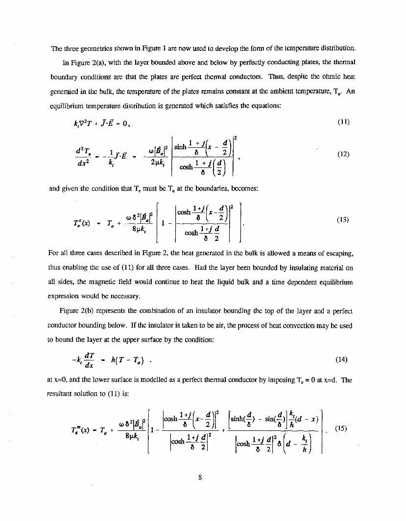
The three geometries shown in Figure 1 are now used to develop the form of the temperature distribution.

In Figure 2(a), with the layer bounded above and below by perfectly conducting plates, the thermal

boundary conditions are that the plates are perfect thermal conductors. Thus, despite the ohmic heat

generated in the bulk, the temperature of the plates remains constant at the ambient temperature, To. An

equilibrium temperature distribution is generated which satisfies the equations:

and given the condition that T, must be To at the boundaries, becomes:

cosh 1 +j d/~ 2

(12)

(13)

For all three cases described in Figure 2, the heat generated in the bulk is allowed a means of escaping,

thus enabling the use of (11) for all three cases. Had the layer been bounded by insulating material

all sides, the magnetic field would continue to heat the liquid bulk and a time dependent equilibrium

expression would be necessary.

Figure 2(b) represents the combination of an insulator bounding the top of the layer and a perfect

conductor bounding below. If the insulator is taken to be air, the process of heat convection may be used

to bound the layer at the upper surface by the condition:

-k, aT It( T - o) (14)

at x=0, and the lower surface is modelled as a perfect thermal conductor by imposing T¢ = 0 at x=d. The

(15)

resultant solution to (11) is:

8

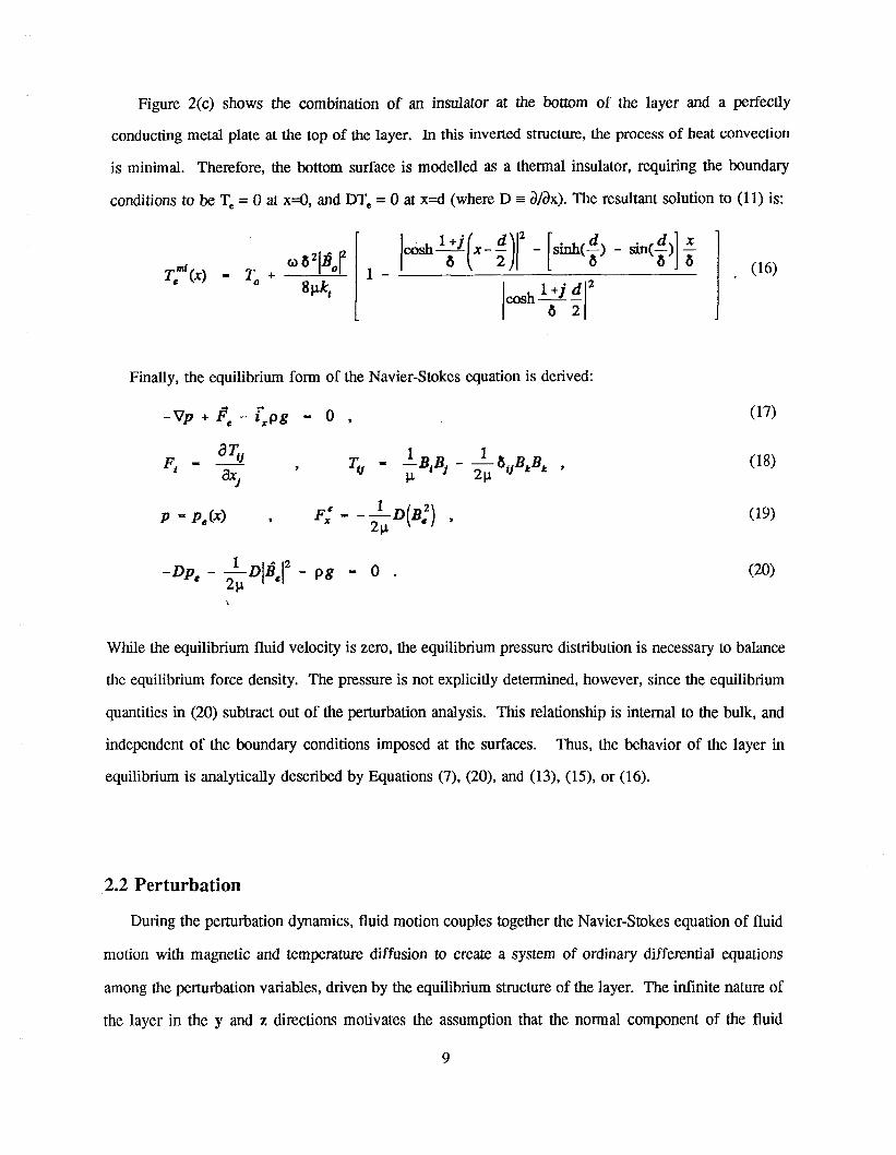
Figure 2(c) shows the combination of an insulator at the bottom of the layer and a perfectly

conducting metal plate at the top of the layer. In this inverted structure, the process of heat convection

is minimal. Therefore, the bottom surface is modelled as a thermal insulator, requiring the boundary

conditions to be T, = 0 at x=0, and DT~ = 0 at x=d (where D -- O/Ox). The resultant solution to (11)

(16)

Finally, the equilibrium form of the Navier-Stokes equation is derived:

(18)

1DB2 (20)

While the equilibrium fluid velocity is zero, the equilibrium pressure distribution is necessary to balance

the equilibrium force density. The pressure is not explicitly determined, however, since the equilibrium

quantities in (20) subtract out of the perturbation analysis. This relationship is internal to the bulk, and

independent of the boundary conditions imposed at the surfaces. Thus, the behavior of the layer in

equilibrium is analytically described by Equations (7), (20), and (13), (15),

2.2 Perturbation

During the perturbation dynamics, fluid motion couples together the Navier-Stokes equation of fluid

motion with magnetic and temperature diffusion to create a system of ordinary differential equations

among the perturbation variables, driven by the equilibrium structure of the layer. The infinite nature of

the layer in the y and z directions motivates the assumption that the normal component of the fluid

9

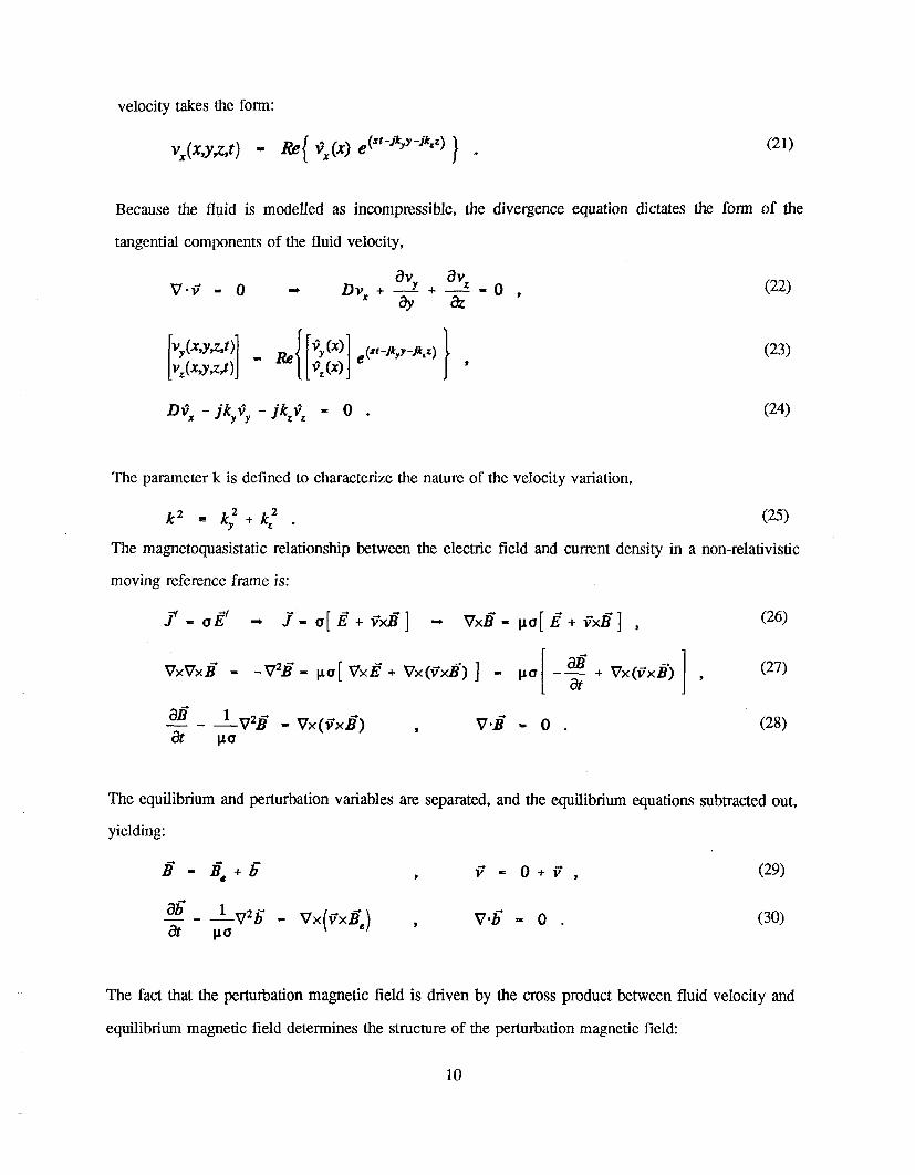
velocity takes the form:

vx(x,y,z,t ) .. (21)

Because the fluid is modelled as incompressible, the divergence equation dictates the form of the

tangential components of the fluid velocity,

av~,V’~ - 0 - /gv x + -- + -- - 0 (22)

ay az ’

(23)

The parameter k is defined to characterize the nature of the velocity variation,

The magnetoquasistatic relationship between the electric field and current density in a non-relativistic

moving reference frame is:

- 0 (28)

The equilibrium and perturbation variables are separated, and the equilibrium equations subtracted out,

yielding:

(29)

, v. r- o (30)

The fact that the perturbation magnetic field is driven by the cross product between fluid velocity and

equilibrium magnetic field determines the structure of the perturbation magnetic field:

10

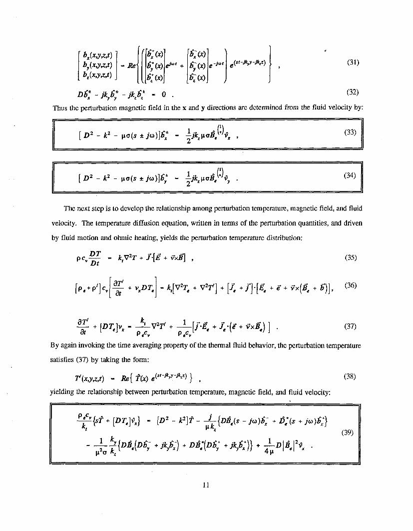
(31)

Thus the perturbation magnetic field in the x and y directions are determined from the fluid velocity by:

(33)

(~)

The next step is to develop the relationship among perturbation temperature, magnetic field, and fluid

velocity. The temperature diffusion equation, written in terms of the perturbation quantities, and driven

by fluid motion and ohmic heating, yields the perturbation temperature distribution:

O T t,,V2r + Y-[~ + ~’~#] , (35)PCv Dt

c [OT~+ vxDT. - kt[V2T.+ V2T¢] + [a~+ f]’[/~. + ~+ Vx(/~. + /~)], (36)

aT~ + [DTe]vx . k~ V2Tt + ll~__[f.ff, e ÷ .~.(~ + ~Tx/~)

(37)~t p eCv p .Cv

By again invoking the time averaging property of the thermal fluid behavior, the perturbation temperature

satisfies (37) by taking the form:

TC(x,y~,t) - Re{ ~(x) (s’-j~7-1~) } ,

yielding the relationship between perturbation temperature, magnetic field, and fluid velocity:

(38)

(39)

11

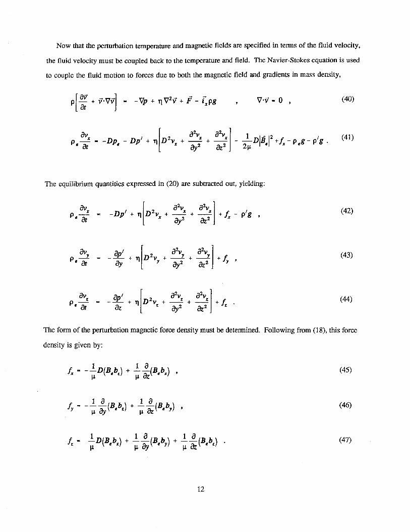
Now that the perturbation temperature and magnetic fields are specified in terms of the fluid velocity,

the fluid velocity must be coupled back to the temperature and field. The Navier-Stokes equation is used

to couple the fluid motion to forces due to both the magnetic field and gradients in mass density,

The equilibrium quantifies expressed in (20) are subtracted out, yidding:

D2v~, + c3y’--’---~ + Oz~ J + f,, - (42)

o~ + ’rl [ D21’y + a),2- + 0-:-:-:-~2 j + "f~ ’

The form of the perturbation magnetic force density must be determined. Following from (18), this force

density is given by:

(4.5)

(47)

12

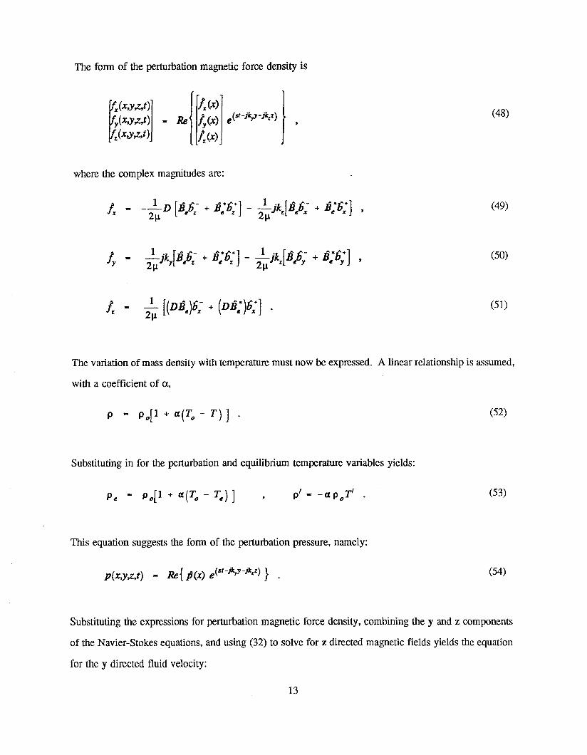
The form of the perturbation magnetic force density is

f,(~,y,z.,t)Ux,y,z,t)

(48)

where the complex magnitudes are:

(50)

(51)

The variation of mass density with temperature must now be expressed. A linear relationship is assumed,

with a coefficient of cq

p - poll + ~(ro - r)] (52)

Substituting in for the perturbation and equilibrium temperature variables yields:

p, - poll + .(to - r,)] , o’- -.Oor’ (53)

This equation suggests the form of the perturbation pressure, namely:

p(x,y~,t) - Re{ fl(x) (st-’%y-#~z) } (54)

Substituting the expressions for perturbation magnetic force density, combining the y and z components

of the Navier-Stokes equations, and using (32) to solve for z directed magnetic fields yields the equation

for the y directed fluid velocity:

13

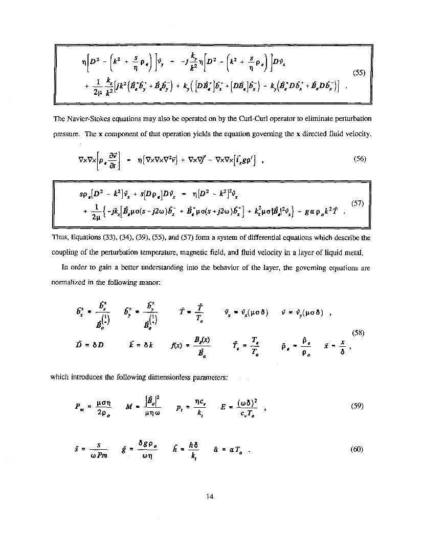
(55)

The Navier-Stokes equations may also be operated on by the Curl-Cud operator to eliminate perturbation

pressure. The x component of that operation yields the equation governing the x directed fluid velocity.

(57)

Thus, Equations (33), (34), (39), (55), and (57) form a system of differential equations which describe

coupling of the perturbation temperature, magnetic field, and fluid velocity in a layer of liquid metal.

In order to gain a better understanding into the behavior of the layer, the governing equations are

normalized in the following manor:

(58)

which introduces the following dimensionless parameters:

(59)

(60)

14

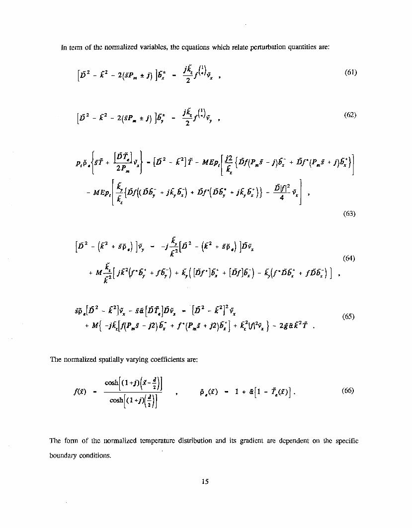
In term of the normalized variables, the equations which relate perturbation quantities are:

4 ’

(63)

(64)

(65)

The normalized spatially varying coefficients are:

cosh[(1 +j)(:¢--~)]

f(:~) " cosh[(l+j)(~)] ’ 15,.) - 1 + ~[1 - /~e(~)]. (66)

The form of the normalized temperature distribution and its gradient are dependent on the specific

boundary conditions.

15

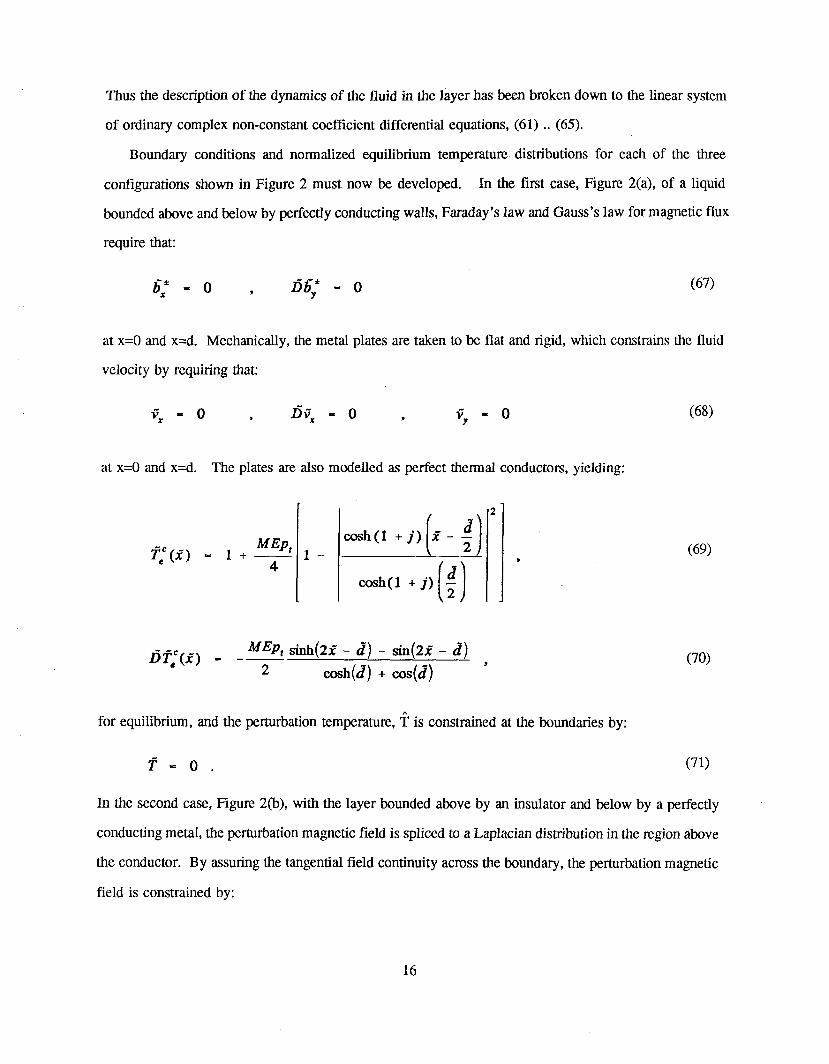
Thus the description of the dynamics of the fluid in the layer has been broken down to the linear system

of ordinary complex non-constant coefficient differential equations, (61) .. (65).

Boundary conditions and normalized equilibrium temperature distributions for each of the three

configurations shown in Figure 2 must now be developed. In the first case, Figure 2(a), of a liquid

bounded above and below by perfectly conducting walls, Faraday’s law and Gauss’s law for magnetic flux

require that:

at x=0 and x=d. Mechanically, the metal plates are taken to be flat and rigid, which constrains the fluid

velocity by requiring that:

at x=0 and x=d. The plates are also modelled as perfect thermal conductors, yielding:

(69)

z~[(:e) Me~,, ~a~(2e - d) - ~(2:e - d) (70)

÷ cos(a)

for equilibrium, and the perturbation temperature, ~ is constrained at the boundaries by:

(71)

In the second case, Figure 2(b), with the layer bounded above by an insulator and below by a perfectly

conducting metal, the perturbation magnetic field is spliced to a Laplacian distribution in the region above

the conductor. By assuring the tangential field continuity across the boundary, the perturbation magnetic

field is constrained by:

16

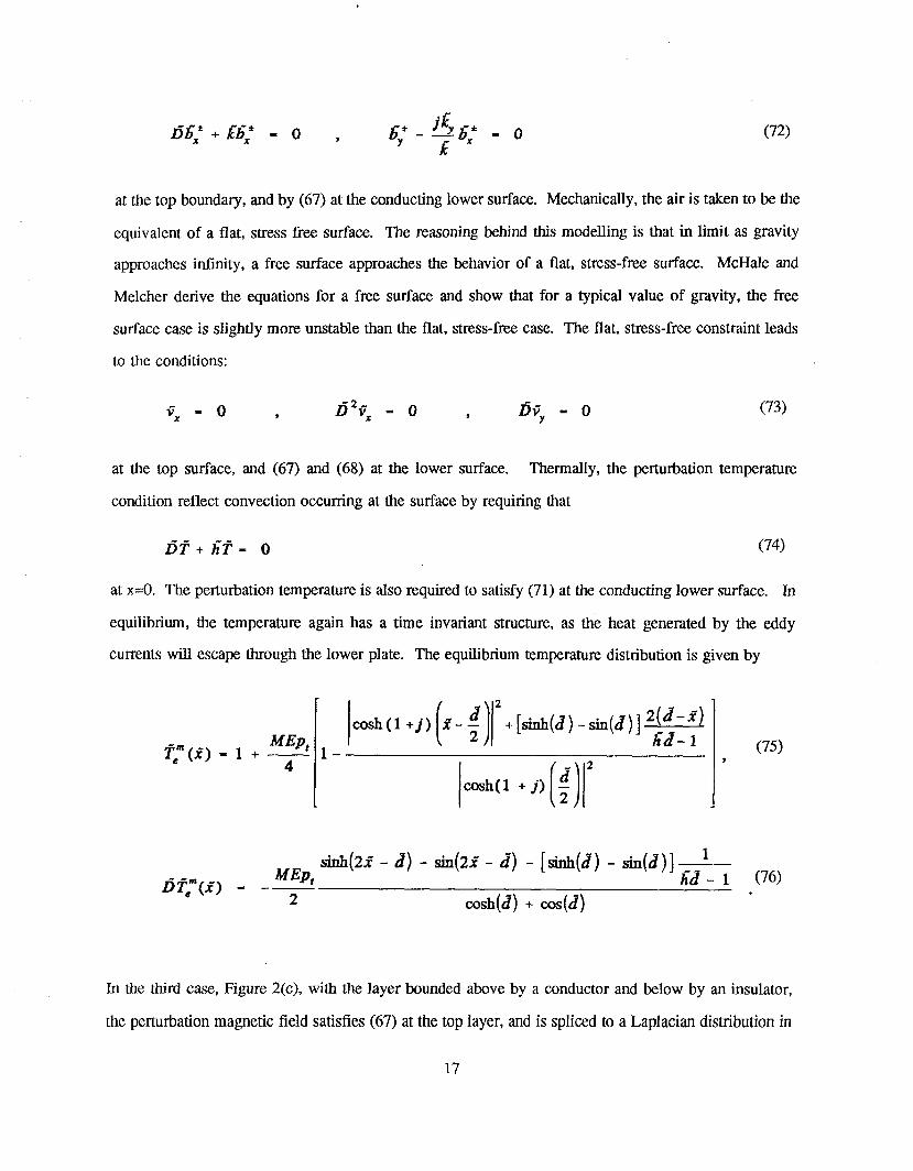
at the top boundary, and by (67) at the conducting lower surface. Mechanically, the air is taken to be the

equivalent of a fiat, stress free surface. The reasoning behind this modelling is that in limit as gravity

approaches infinity, a free surface approaches the behavior of a fiat, stress-free surface. McHale and

Melcher derive the equations for a free surface and show that for a typical value of gravity, the free

surface case is slightly more unstable than the fiat, stress-free case. The fiat, stress-free constraint leads

to the conditions:

~ - 0 , /~2#~ . 0 , /~Ty - 0 (73)

at the top surface, and (67) and (68) at the lower surface. Thermally, the perturbation temperature

condition reflect convection occurring at the surface by requiring that

(74)

at x=0. The perturbation temperature is also required to satisfy (71) at the conducting lower surface.

equilibrium, the temperature again has a time invariant structure, as the heat generated by the eddy

currents will escape through the lower plate. The equilibrium temperature distribution is given by

t- 1 + -4.

cosh ( 1(75)

sinh(2:~- d) - sin(2:~- d) -[sinh(d) - sin(d)]--MEpt /~d- 1 (76)

In the third case, Figure 2(c), with the layer bounded above by a conductor and below by an insulator,

the perturbation magnetic field satisfies (67) at the top layer, and is spliced to a Laplacian distribution

17

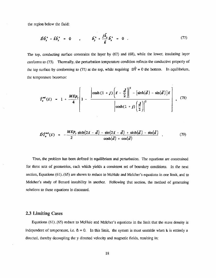
the region below the fluid:

The top, conducting surface constrains the layer by (67) and (68), while the lower, insulating layer

conforms to (73). Thermally, the perturbation temperature condition reflects the conductive property

the top surface by conforming to (71) at the top, while requiring D’~ = 0 the bottom. In equilibrium,

the temperature becomes:

~(~) = 1 + 4

_d(78)

1~,"(.~) MEp, sinh(22 - d) - sin(2:~ - d) + sirda(d) - sin(d) (79)

Thus, the problem has been defined in equilibrium and perturbation. The equations are constrained

for three sets of geometries, each which yields a consistent set of boundary conditions. In the next

section, Equations (61)..(65) are shown to reduce to McHale and Melcher’s equations in one limit, and

Melcher’s study of Benard instability in another. Following that section, the method of generating

solutions to these equations is discussed.

2.3 Limiting Cases

Equations (61)..(65) reduce to McHale and Melcher’s equations in the limit that the mass density

independent of temperature, i.e. ~ = 0. In this limit, the system is most unstable when k is entirely z

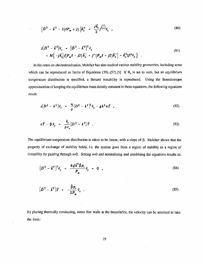
directed, thereby decoupling the y directed v~locity and magnetic fields, resulting in:

18

¯ " 1

T~ )(80)

+ M{ -j~=[f(P.#- j2)~x- + f*(P.g + j2)~’x+] + /~l]]z#~

In his notes on elecffomech~cs, Melcher h~ Mm s~died v~ous s~bility geome~es, ~cluding ~me

which c~ ~ reproduced ~ limits of Equations (39)..(57).[5] o i s ~t t o ~B, but ~ equi librium

tempera~ distribution is s~cifi~, a Benard ~stability is repBdu~d. Using ~e Boussinesque

approximation of keeping ~e equi~bfium m~s density cons~t in~ese equations, ~e following ~uatiom

result:

The equilibrium temperature distribution is taken to be linear, with a slope of I~. Melcher shows that the

property of exchange of stability holds, i.e. the system goes from a region of stability to a region of

instability by passing through s=0. Setting s---O and normalizing and combining the equations results in:

By placing thermally conducting, stress free walls at the boundaries, the velocity can be assumed to take

the form:

19

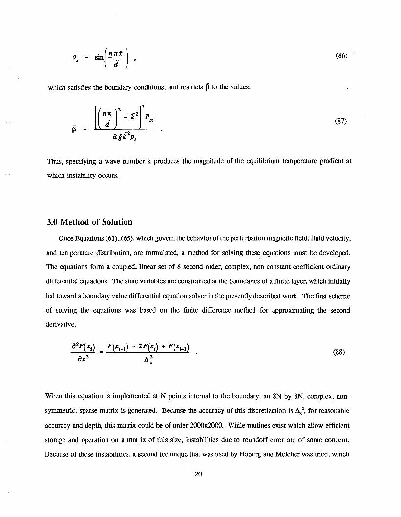
(86)

which satisfies the boundary conditions, and restricts ~ to the values:

(87)

Thus, specifying a wave number k produces the magnitude of the equilibrium temperature gradient at

which instability occurs.

3.0 Method of Solution

Once Equations (61)..(65), which govern the behavior of the perturbation magnetic field, fluid velocity,

and temperature distribution, are formulated, a method for solving these equations must be developed.

The equations form a coupled, linear set of 8 second order, complex, non-constant coefficient ordinary

differential equations. The state variables are constrained at the boundaries of a finite layer, which initially

led toward a boundary value differential equation solver in the presently described work. The first scheme

of solving the equations

derivative,

was based on the finite difference method for approximating the second

When this equation is implemented at N points internal to the boundary, an 8N by 8N, complex, non-

symmetric, sparse matrix is generated. Because the accuracy of this discretization is Ax2, for reasonable

accuracy and depth, this matrix could be of order 2000x2000. While routines exist which allow efficient

storage and operation on a matrix of this size, instabilities due to roundoff error are of some concem.

Because of these instabilities, a second technique that was used by Hoburg and Melcher was tried, which

20

involves a fourth order Runge-Kutta method.[6] Since Equations (61)..(65) take the form:

DyI - f~(x, yl,...,y,~) 1 < i ,:16 , (89)

the Runge Kutta method determines yi(x+h) given yi(x)

koi - hf~(x, yl ..... Yl~)

k~ - hf~x+ i,y~ ÷~,...,y~+ ~ ,

k=~ - hAx+py~ +~,...,yz~ +~ ,

1k

(9O)

The value yi(x) is then replaced with yi(x+d) and in this way the equations are integrated across the layer.

Because this system is linear, the relationship between Y at the boundary x=d and Y at x=0 may be

expressed as:

L r o - r~ (91)

By individually setting each y~ at x=0 to one with all others set to zero and integrating across the layer

to get Y at x=d, column i of matrix L is filled. The columns Yo and Yd are then transformed to vectors

whose specific forms are dependent on the form of the boundary conditions. Specifically, the upper half

of Yo is transformed into the combinations of state variables which are constrained to be zero at x=0,

while the lower half remains state variables which are left unconstrained at x=0. This transformation can

be represented as multiplying Yo by matrix R. Similarly, Yd is transformed by matrix Q, becoming

partitioned into a vector whose top half is a combination of state variables which are constrained to be

zero at x=d, and whose lower half are unconstrained at x=d.

For example, consider Equations (80) and (81), which McHale and Melcher investigated. The state

variables are:

21

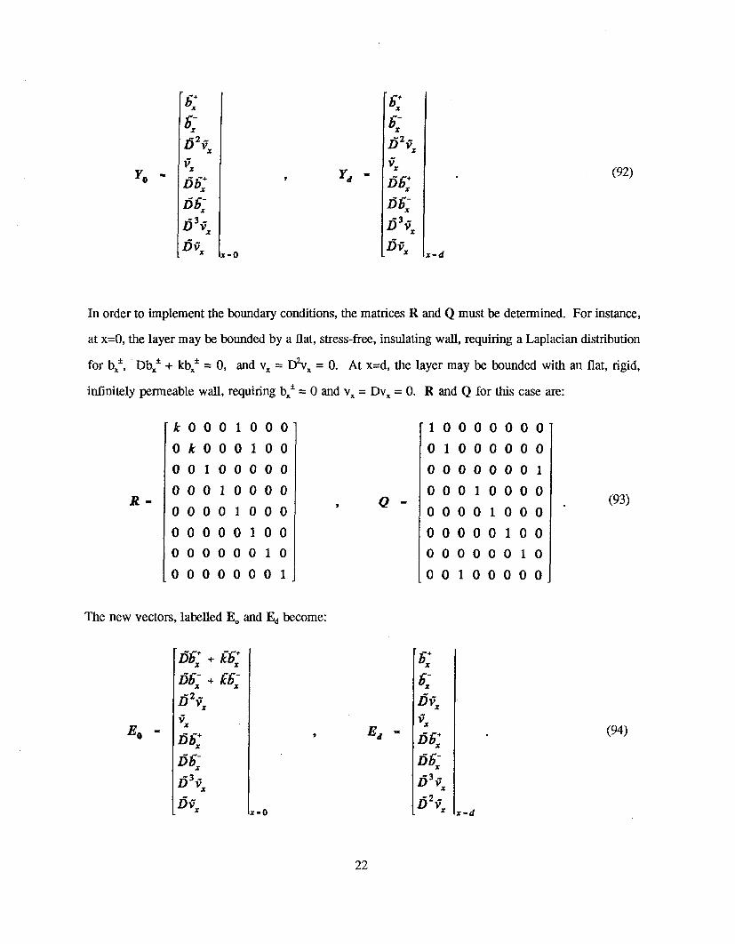
(92)

In order to implement the boundary conditions, the matrices R and Q must be determined. For instance,

at x=0, the layer may be bounded by a flat, stress-free, insulating wall, requiring a Laplacian distribution

for bx~, Db~ + kbx± = 0, and Vx = D~vx = 0. At x=d, the layer may be bounded with an fiat, rigid,

infinitely permeable wall, requiring bx± = 0 and v~ = Dvx = 0. R and Q for this case are:

k0001000

0k000100

00100000

00010000

00001000

00000100

00000010

00000001

10000000

01000000

00000001

00010000

00001000

00000100

00000010

00100000

(93)

The new vectors, labelled Eo and Ed become:

Ell Ed ’- (94)

22

4.0 Results

The results of the implementation of the solution method on Equations (61)..(65) are described in

section.

4.1 Experimental Parameter Values

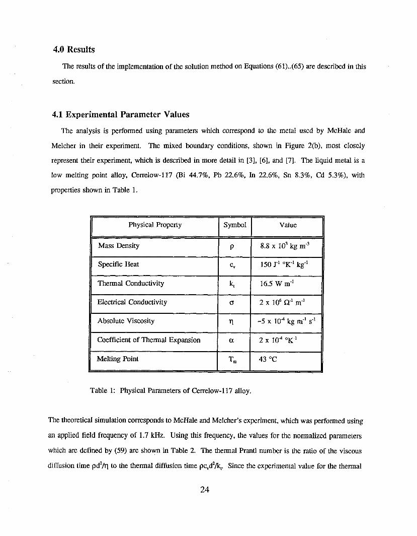
The analysis is performed using parameters which correspond to the metal used by McHale and

Melcher in their experiment. The mixed boundary conditions, shown in Figure 2(b), most closely

represent their experiment, which is described in more detail in [3], [6], and [7]. The liquid metal is a

low melting point alloy, Cerrelow-ll7 (Bi 44.7%, Pb 22.6%, In 22.6%, Sn 8.3%, Cd 5.3%), with

properties shown in Table 1.

Physical Property Symbol Value

Mass Density 9 8.8 x 103 kg m-3

Specific Heat cv 150 j-1 OK-1 kg-1

Thermal Conductivity kt 16.5 W m-~

Electrical Conductivity t~ 2 x 106 ~)~ -a

Absolute Viscosity rl -5 x 10~ kg m1 st

Coefficient of Thermal Expansion t~ 2 x 10-~ °K-1

Melting Point Tm 43 °C

Table 1: Physical Parameters of Cerrelow-117 alloy.

The theoretical simulation corresponds to McHale and Melcher’s experiment, which was performed using

an applied field frequency of 1.7 kHz. Using this frequency, the values for the normalized parameters

which are defined by (59) are shown in Table 2. The thermal Prantl number is the ratio of the viscous

diffusion time pd2/rl to the thermal diffusion time pcvd2/kt. Since the experimental value for the thermal

24

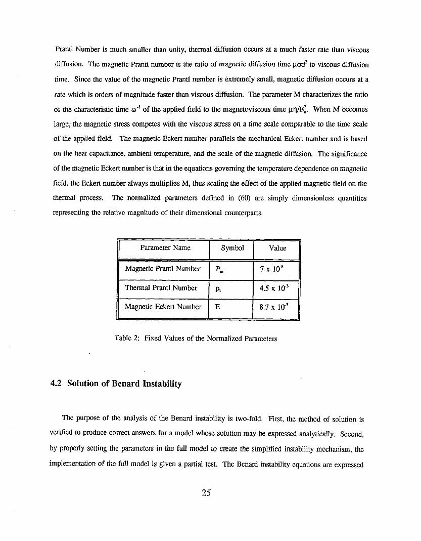
Pranfl Number is much smaller than unity, thermal diffusion occurs at a much faster rate than viscous

diffusion. The magnetic Prantl number is the ratio of magnetic diffusion lime gcrd2 to viscous diffusion

time. Since the value of the magnetic Prantl number is extremely small, magnetic diffusion occurs at a

rate which is orders of magnitude faster than viscous diffusion. The parameter M characterizes the ratio

of the characteristic time ~~ of the applied field to the magnetoviscous time grl/B.2. When M becomes

large, the magnetic stress competes with the viscous stress on a time scale comparable to the time scale

of the applied field. The magnetic Eckert number parallels the mechanical Eckert number and is based

on the heat capacitance, ambient temperature, and the scale of the magnetic diffusion. The significance

of the magnetic Eckert number is that in the equations governing the temperature dependence on magnetic

field, the Eckert number always multiplies M, thus scaling the effect of the applied magnetic field on the

thermal process. The normalized parameters def’med in (60) are simply dimensionless quantities

representing the relative magnitude of their dimensional counterparts.

Parameter Name Symbol Value

Magnetic Prantl Number Pm 7 x 10.8

Thermal Prantl Number Pt 4.5 x lffs

Magnetic Eckert Number E 8.7 x 10-~

Table 2: Fixed Values of the Normalized Parameters

4.2 Solution of Benard Instability

The purpose of the analysis of the Benard instability is two-fold. First, the method of solution is

verified to produce correct answers for a model whose solution may be expressed analytically. Second,

by properly setting the parameters in the full model to create the simplified instability mechanism, the

implementation of the full model is given a partial test. The Benard instability equations are expressed

25

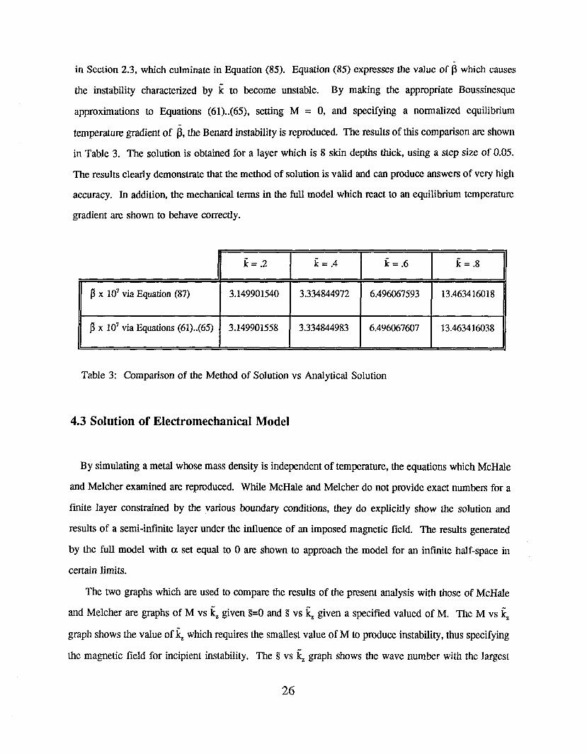
in Section 2.3, which culminate in Equation (85). Equation (85) expresses the value of I~ which causes

the instability characterized by ~ to become unstable. By making the appropriate Boussinesque

approximations to Equations (61)..(65), setting M = 0, and specifying a normalized equilibrium

temperature gradient of 1~, the Benard instability is reproduced. The results of this comparison are shown

in Table 3. The solution is obtained for a layer which is 8 skin depths thick, using a step size of 0.05.

The results clearly demonstrate that the method of solution is valid and can produce answers of very high

accuracy. In addition, the mechanical terms in the full model which react to an equilibrium temperature

gradient are shown to behave correctly.

~ x 107 via Equation (87) 3.149901540 3.334844972 6.496067593 13.463416018

~ X 107 via Equations (61)..(65) 3.149901558 3.334844983 6.496067607 13.463416038

Table 3: Comparison of the Method of Solution vs Analytical Solution

4.3 Solution of Electromechanical Model

By simulating a metal whose mass density is independent of temperature, the equations which McHale

and Melcher examined are reproduced. While McHale and Melcher do not provide exact numbers for a

finite layer constrained by the various boundary conditions, they do explicitly show the solution and

results of a semi-infinite layer under the influence of an imposed magnetic field. The results generated

by the full model with ¢x set equal to 0 are shown to approach the model for an infinite half-space in

certain limits.

The two graphs which are used to compare the results of the present analysis with those of McHale

and Melcher are graphs of M vs ~ given ~-0 and ~ vs ~ given a specified valued of M. The M vs ~

graph shows the value of f~ which requires the smallest value of M to produce instability, thus specifying

the magnetic field for incipient instability. The ~ vs ~ graph shows the wave number with the largest

26

growth rate for a given value of applied magnetic field, and depending on the sign of this growth rate,

whether or not the mode is stable.

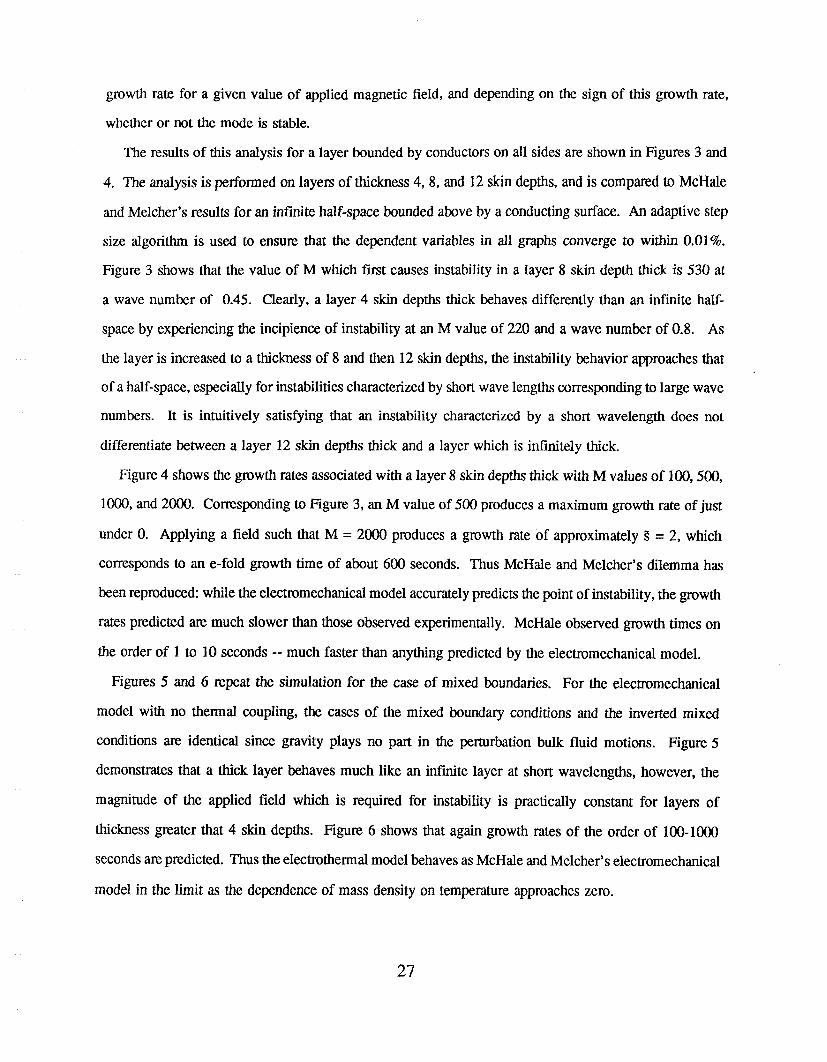
The results of this analysis for a layer bounded by conductors on all sides are shown in Figures 3 and

4. The analysis is performed on layers of thickness 4, 8, and 12 skin depths, and is compared to McHale

and Melcher’s results for an inlrmite half-space bounded above by a conducting surface. An adaptive step

size algorithm is used to ensure that the dependent variables in all graphs converge to within 0.01%.

Figure 3 shows that the value of M which first causes instability in a layer 8 skin depth thick is 530 at

a wave number of 0.45. Clearly, a layer 4 skin depths thick behaves differently than an infinite half-

space by experiencing the incipience of instability at an M value of 220 and a wave number of 0.8. As

the layer is increased to a thickness of 8 and then 12 skin depths, the instability behavior approaches that

of a half-space, especially for instabilities characterized by short wave lengths corresponding to large wave

numbers. It is intuitively satisfying that an instability characterized by a short wavelength does not

differentiate between a layer 12 skin depths thick and a layer which is infinitely thick.

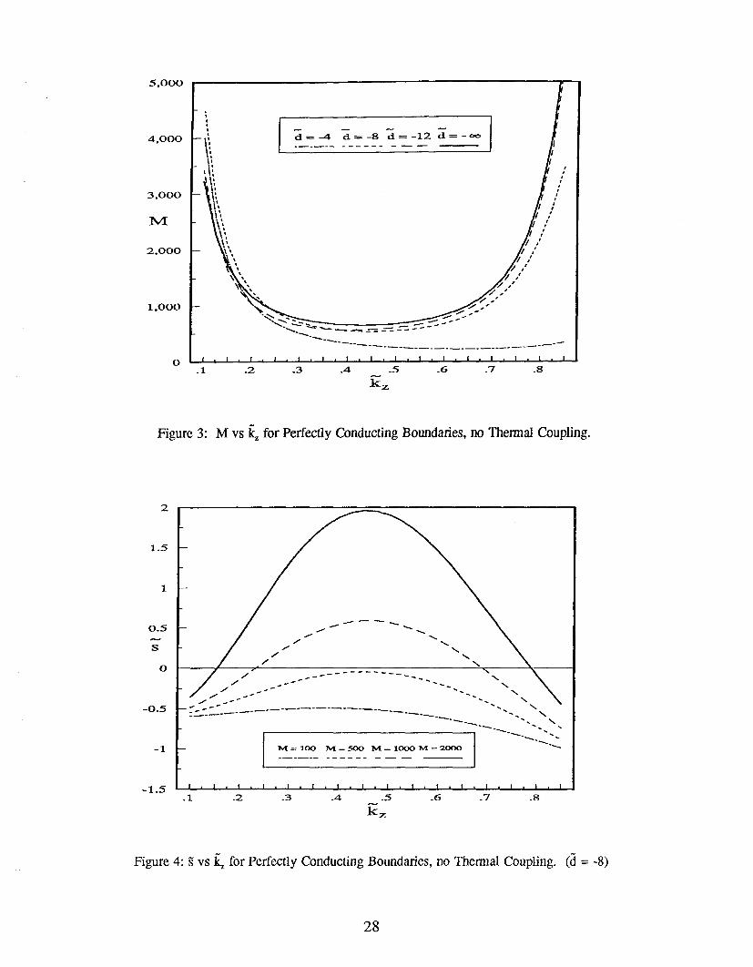
Figure 4 shows the growth rates associated with a layer 8 skin depths thick with M values of 100, 500,

1000, and 2000. Corresponding to Figure 3, an M value of 500 produces a maximum growth rate of just

under 0. Applying a field such that M = 2000 produces a growth rate of approximately ~ = 2, which

corresponds to an e-fold growth time of about 600 seconds. Thus McHale and Melcher’s dilemma has

been reproduced: while the electromechanical model accurately predicts the point of instability, the growth

rates predicted are much slower than those observed experimentally. McHale observed growth times on

the order of 1 to 10 seconds -- much faster than anything predicted by the electromechanical model.

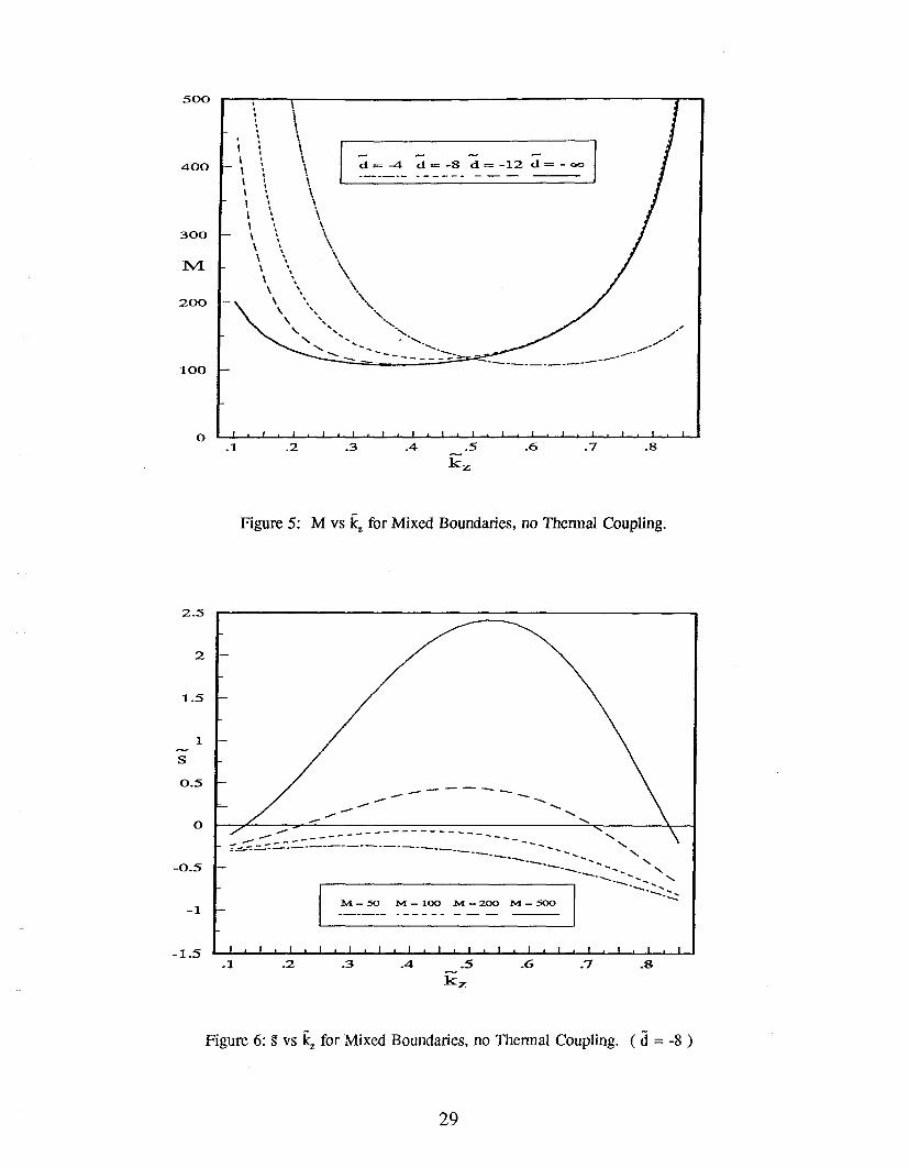
Figures 5 and 6 repeat the simulation for the case of mixed boundaries. For the electromechanical

model with no thermal coupling, the cases of the mixed boundary conditions and the inverted mixed

conditions are identical since gravity plays no part in the perturbation bulk fluid motions. Figure 5

demonstrates that a thick layer behaves much like an infinite layer at short wavelengths, however, the

magnitude of the applied field which is required for instability is practically constant for layers of

thickness greater that 4 skin depths. Figure 6 shows that again growth rates of the order of 100-1000

seconds are predicted. Thus the electrothermal model behaves as McHale and Melcher’s electromechanical

model in the limit as the dependence of mass density on temperature approaches zero.

27

5,000

4,000

3,OOO

M

2,000

1.000

0

Figure 3: M vs ~, for Perfectly Conducting Boundaries, no Thermal Coupling.

2

0.5

S

0

-1 M=IO0 M=ff~O0 M = i000 M = 2000

kz

Figure 4: ~ vs ~ for Perfectly Conducting Boundaries, no Thermal Coupling. (~ = -8)

28

500

400

300

M

200

100

kz

Figure 5: M vs 1~ for Mixed Boundaries, no Thermal Coupling.

2.5

2

1.5

1

0.5

0

-0.5

-1

-1.5

M=50 M=IO0 M=200

l . I . I . I , I , I , I , I , I , I , I , I . ! . I , I , I.1 .2 .3 .4 .5 .6 .7

kz

Figure 6: g vs ~ for Mixed Boundaries, no Thermal Coupling. ( ~ = -8

29

4.4 Solution of the Electrothermal Model

In the electromechanical model without thermal coupling, it is possible to analytically determine that

the critical condition for a given value of ~ occurs when fc is entirely z directed. This is demonstrated

by rearranging the governing equations into a single equation in % In this equation, all occurrences of

M are multiplied by ~; thus ~ essentially scales the value of the applied magnetic field. The added

complexity of the thermally coupled equations precludes such a method. However simulations of the

electrothermal process show that for a given value of [, the lowest value of M required for instability

occurs when ~ is entirely z directed. Therefore ~ is set to 0, which decouples the y directed velocity and

magnetic field from the temperature and x directed velocity and magnetic field, and temperature. This

realization reduces the order of the system from a set of 8 to a set of 5 second order differential equations.

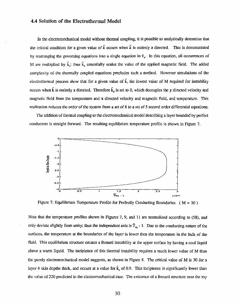
The addition of thermal coupling to the electromechanical model describing a layer bounded by perfect

conductors is straight forward. The resulting equilibrium temperature profile is shown in Figure 7.

-0.5

-1

-2

-2.5

-3

-3.5

0

Te.q - 1 xlO--#,

Figure 7: Equilibrium Temperature Profile for Perfectly Conducting Boundaries. ( M = 30

Note that the temperature profiles shown in Figures 7, 9, and 11 are normalized according to (58), and

only deviate slightly from unity; thus the independent axis is ff’,~ - l. Due to the conducting nature of the

surfaces, the temperature at the boundaries of the layer is lower then the temperature in the bulk of the

fluid. This equilibrium structure creates a Benard instability at the upper surface by having a cool liquid

above a warm liquid. The incipience of this thermal instability requires a much lower value of M than

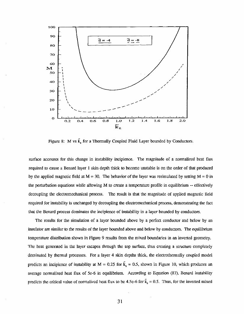
the purely electromechanicat model suggests, as shown in Figure 8. The critical value of M is 30 for a

layer 4 skin depths thick, and occurs at a value for ~ of 0.9. This incipience is significantly lower than

the value of 220 predicted in the electromechanical case. The existence of a Benard structure near the top

3O

1.00

90

80

70

6o

M~0

.40

30

20

10

00.2 0.4 0.6 0.8 1.0 1.2 1.4 1.6 1.8 2.0

Figure 8: M vs ~ for a Thermally Coupled Fluid Layer bounded by Conductors.

surface accounts for this change in instability incipience. The magnitude of a normalized heat flux

required to cause a Benard layer 1 skin depth thick to become unstable is on the order of that produced

by the applied magnetic field at M = 30. The behavior of the layer was resimulated by setting M = 0 in

the perturbation equations while allowing M to create a temperature profile in equilibrium -- effectively

decoupling the electromechanical process. The result is that the magnitude of applied magnetic field

required for instability is unchanged by decoupling the electromechanical process, demonstrating the fact

that the Benard process dominates the incipience of instability in a layer bounded by conductors.

The results for the simulation of a layer bounded above by a perfect conductor and below by an

insulator are similar to the results of the layer bounded above and below by conductors. The equilibrium

temperature distribution shown in Figure 9 results from the mixed boundaries in an inverted geometry.

The heat generated in the layer escapes through the top surface, thus creating a structure completely

dominated by thermal processes. For a layer 4 skin depths thick, the electrothermally coupled model

predicts an incipience of instability at M = 0.25 for ~ = 0.5, shown in Figure 10, which produces an

average normalized heat flux of 5e-6 in equilibrium. According to Equation (87), Benard instability

predicts the critical value of normalized heat flux to be 4.5e-6 for ~ = 0.5. Thus, for the inverted mixed

31

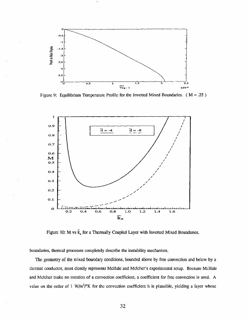
Figure 9: Equilibrium Temperature Profile for the Inverted Mixed Boundaries. ( M = .25

1

0.9

0.8

0.7

0.6

M0.5

0.4

0.3

0.2

0.1

0

II

!

~_ =_ ± ? = -~_ /’/

//

/

\ / /

0.2 0.4 0.6 0.8 1.0 1.2 1.4 1.6

Figure 10: M vs ~ for a Thermally Coupled Layer with Inverted Mixed Boundaries.

boundaries, thermal processes compIetely describe the instability mechanism.

The geometry of the mixed boundary conditions, bounded above by free convection and below by a

thermal conductor, most closely represents McHale and Melcher’s experimental setup. Because McHale

and Melcher make no mention of a convection coefficient, a coefficient for free convection is used. A

value on the order of 1 W/m:/°K for the convection coefficient h is plausible, yielding a layer whose

32

behavior is identical to the behavior of a layer bounded above by a perfect insulator. The temperature

prof’de in equilibrium is then simply the inverse of Figure 9, producing an equilibrium structure which is

very stable. An accurate M vs ~ plot becomes numerically difficult because the lowest value for M at

which instability occurs is on the order of 1000130, compared to a value of 106 for McHale and Melcher’s

electromechanical model.

A comparison of growth rates for the various thermal cases is inherently difficult due to the fact that

the point of instability has been significantly altered in each case. For example, in order to compare

growth rates for conducting boundaries, a value of M above 220 would be necessary. However, at

M = 220, the growth rate of the thermally coupled layer is already very large due to the fact that the

process of electrothermal coupling becomes unstable at M = 30. This difficulty is especially true for an

inverted set of mixed boundaries, with a range of critical M from 0.25 for the electrothermal model to 106

for the electromechanical model. The same phenomena occurs for the case of mixed boundaries, only

reversed; the electromechanical model becomes unstable at a much lower value of M than the prediction

of the thermally coupled model.

Figure 11:

o

-0.5

-1

-1.5

-2.5

-3

-3.5

-40

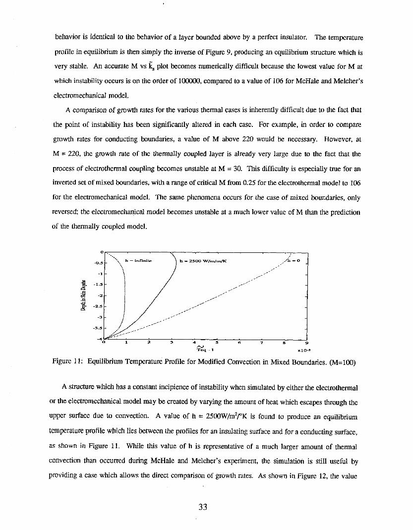
Equilibrium Temperature Profile for Modified Convection in Mixed Boundaries. (M=100)

A structure which has a constant incipience of instability when simulated by either the electrothermal

or the electromechanical model may be created by varying the amount of heat which escapes through the

upper surface due to convection. A value of h = 2500W/m2/°K is found to produce an equilibrium

temperature profile which lies between the profiles for an insulating surface and for a conducting surface,

as shown in Figure 11. While this value of h is representative of a much larger amount of thermal

convection than occurred during McHale and Melcher’s experiment, the simulation is still useful by

providing a case which allows the direct comparison of growth rates. As shown in Figure 12, the value

33

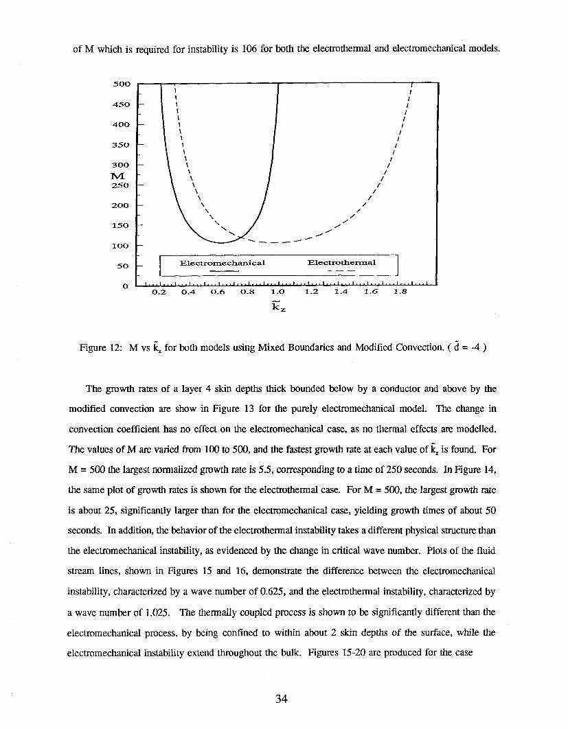
of M which is required for instability is 106 for both the electrothermal and electromechanical models.

500

450

400

350

30O

M250

200

150

1OO

5O

O

IIIII

/I/

//

!/

/

Electromechanical Electrothermal I

0.2 0.4 0.6 0.8 1 .O 1.2 1.4 1.6 1.8

kz

Figure 12: M vs ~ for both models using Mixed Boundaries and Modified Convection. ( ~ = -4

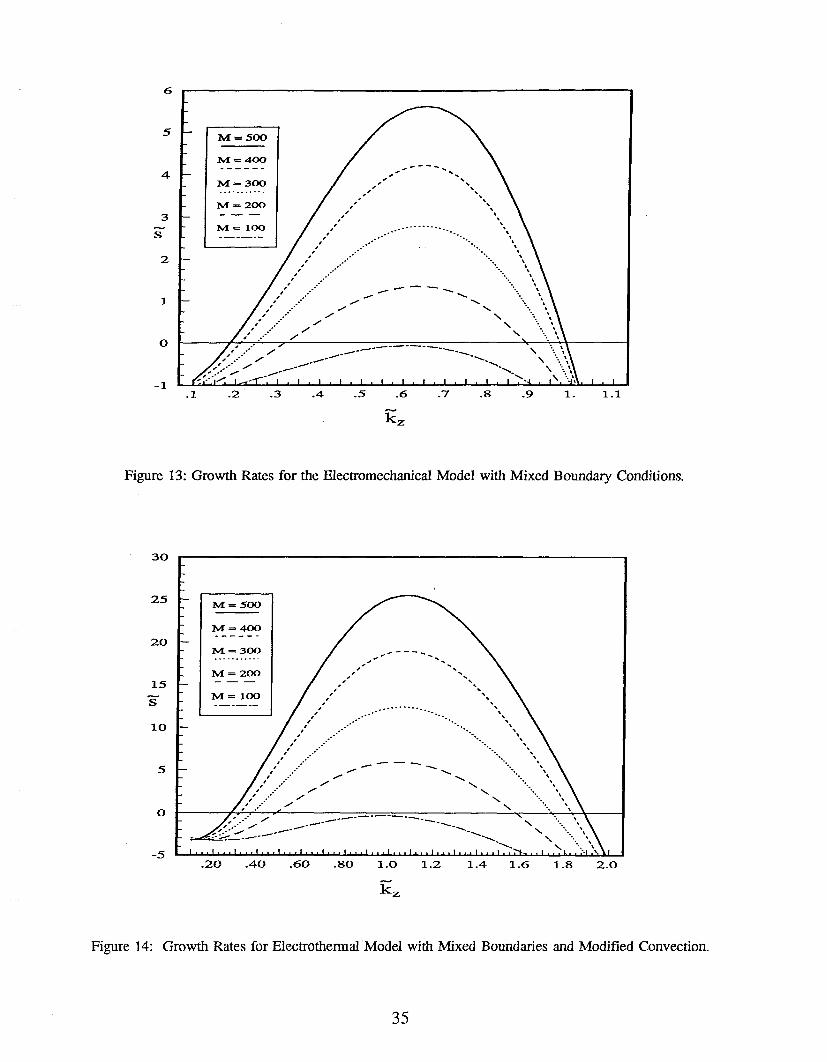
The growth rates of a layer 4 skin depths thick bounded below by a conductor and above by the

modified convection are show in Figure 13 for the purely electromechanical model. The change in

convection coefficient has no effect on the electromechanical case, as no thermal effects are modelled.

The values of M are varied from 100 to 500, and the fastest growth rate at each value of~ is found. For

M = 500 the largest normalized growth rate is 5.5, corresponding to a time of 250 seconds. In Figure 14,

the same plot of growth rates is shown for the electrothermal case. For M = 500, the largest growth rate

is about 25, significantly larger than for the electromechanical case, yielding growth times of about 50

seconds. In addition, the behavior of the electrothermal instability takes a different physical structure than

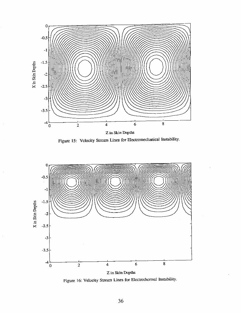
the electromechanical instability, as evidenced by the change in critical wave number. Plots of the fluid

stream lines, shown in Figures 15 and 16, demonstrate the difference between the electromechanical

instability, characterized by a wave number of 0.625, and the electrothermal instability, characterized by

a wave number of 1.025. The thermally coupled process is shown to be significantly different than the

electromechanical process, by being confined to within about 2 skin depths of the .surface, while the

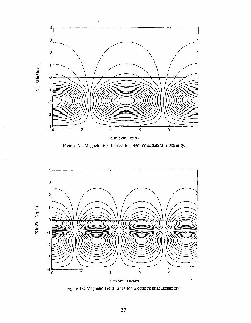
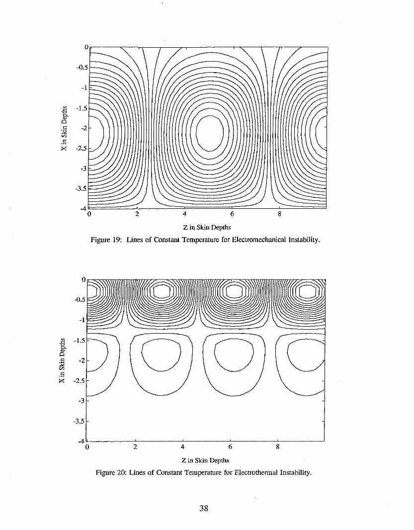
electromechanical instability extend throughout the bulk. Figures 15-20 are produced for the case

34

6

5

4

2

1

0

-1

Figure I3: Growth Rates for the Electromechanical Model with Mixed Boundary Conditions.

30

25

20

15

S

10

5

0

-5.20 .40 .60 .80 1.0 1.2 1.4 1.6 1.8 2.0

Figure 14: Growth Rates for Electrothermal Model with Mixed Boundaries and Modified Convection.

35

-0.5

-1

-3

-3.5

2 4 ; ~

Z in Skin Depths

Figure 15: Velocity Stream Lines for Electromechanical Instability.

0

-0.5

-1

-1.5

-2

-2.5

-3

-3.5

0 2 4 6 8

Z in Skin Depths

Figure 16: Velocity Stream Lines for Electrothermal Instability.

36

4

-2

-3

Figure 17:

4 6 8

Z in Skin Depths

Magnetic Field Lines for Electromechanical Instability.

-1

-2

-3

-4 i0 2 4 6 8

Z in Skin Depths

Figure 18: Magnetic Field Lines for Electrothermal Instability.

37

0

Figure 19:

2 4 6 8

Z in Skin Depths

Lines of Constant Temperature for Electromechanical Instability.

0

0 2 4 6 8

Z in Skin Depths

Figure 20: Lines of Constant Temperature for Electrothermal Instability.

38

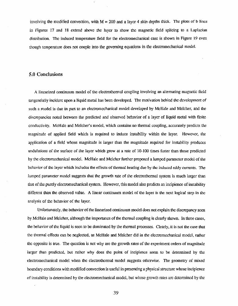
involving the modified convection, with M = 200 and a layer 4 skin depths thick. The plots of b lines

in Figures 17 and 18 extend above the layer to show the magnetic field splicing to a Laplacian

distribution. The induced temperature field for the electromechanical case is shown in Figure 19 even

though temperature does not couple into the governing equations in the electromechanical model.

5.0 Conclusions

A linearized continuum model of the electrothermal coupling involving an alternating magnetic field

tangentially incident upon a liquid metal has been developed. The motivation behind the development of

such a model is due in part to an electromechanical model developed by McHale and Melcher, and the

discrepancies noted between the predicted and observed behavior of a layer of liquid metal with finite

conductivity. McHale and Melcher’s model, which contains no thermal coupling, accurately predicts the

magnitude of applied field which is required to induce instability within the layer. However, the

application of a field whose magnitude is larger than the magnitude required for instability produces

undulations of the surface of the layer which grow at a rate of 10-100 times faster than those predicted

by the electromechanical model. McHale and Melcher further proposed a lumped parameter model of the

behavior of the layer which includes the effects of thermal heating due by the induced eddy currents. The

lumped parameter model suggests that the growth rate of the electrothermal system is much larger than

that of the purely electromechanical system. However, this model also predicts an incipience of instability

different than the observed value. A linear continuum model of the layer is the next logical step in the

analysis of the behavior of the layer.

Unfortunately, the behavior of the linearized continuum model does not explain the discrepancy seen

by McHale and Melcher, although the importance of the thermal coupling is clearly shown. In three cases,

the behavior of the liquid is seen to be dominated by the thermal processes. Clearly, it is not the case that

the thermal effects can be neglected, as McHale and Melcher did in the electromechanical model, rather

the opposite is true. The question is not why are the growth rates of the experiment orders of magnitude

larger than predicted, but rather why does the point of incipience seem to be determined by the

electromechanical model when the electrothermal model suggests otherwise. The geometry of mixed

boundary conditions with modified convection is useful in presenting a physical structure whose incipience

of instability is determined by the electromechanical model, but whose growth rates are determined by the

39

electrothermal coupling. The modified convection coefficient, however, does not explain the dilemma

proposed by McHale and Melcher, for without some extraordinary apparatus for heat transport, the layer

which was studied does not induce convection at such a large rate.

An analysis of the assumptions taken in the development of the continuum model should shed some

light on the proposed dilemma. In both equilibrium and perturbation, a time-averaging property was

assumed which allows terms which vary at twice the frequency of the applied field to be neglected. The

surface undulations which McHale and Melcher observed oscillated at a frequency of .5 to 2 Hz under

the application of a field at 2 kHz. This observation supports the assumption of the time averaging

property. The magnetoquasistatic form of Maxwell’s equations are used, thus neglecting the role of

displacement current. This assumption is well justified since the phenomenon of wave propagation is

negligible at frequencies in the kHz range. The variation of the fluid velocity in the directions tangential

to the surface of the layer is assumed to be sinusoidal, which is reasonable because the existence of finite

boundaries will serve only to discretize the allowable wave numbers.

The remaining assumption used in the development of the continuum model is that of linearity.

Specifically, all multiplication of perturbation quantities are neglected in the development of

Equations (61)..(65). This was done on the assumption that the perturbation quantities would be orders

of magnitude less than those in equilibrium. However, the non-linear coupling seems to account for a

significant aspect of the fluid behavior. Specifically, in explanation of McHale and Melcher’s dilemma,

a qualitative argument would be that despite the fact that the linear model predicts a very stable structure,

the non-linear coupling between the magnetic forces and fluid velocity cause instability at a value of

applied field predicted by the linear electromechanical model. Once fluid motion begins, the process of

Benard instability together with the non-linear coupling drive the instability at rate which is much larger

than predicted by either linear model. This explanation is supported by the fact that for a structure whose

incipience of instability is consistent between the electromechanical and the electrothermal models, the

thermally coupled model predicts much faster growth rates.

The implications of this conclusion are quite significant. With the addition of non-linear thermal

coupling necessary to accurately model the system, the prior assumption that the behavior of the layer is

dominated by a surface coupled model is shown to be unfounded. This analysis has shown that a

complicated, probably non-linear, thermally coupled bulk analysis is necessary to adequately describe the

fluid behavior. Future research will have to account for these non-linear effects to determine how other

systems of low frequency and finite conductivity behave.

4O

References

Shigeo Asai. Birth and recent activities of electromagnetic processing of materials.

ISIJ International, 29(12):981-992, 1989.

Fugate, David W. Two-dimensional surface-coupled modeling of electromagnetic

levitation of liquid metals. PhD thesis, Department of Electrical and Computer

Engineering, Camegie Mellon University. 1990.

McHale, E. J. & Melcher, J. R., Instability of a planar liquid in an alternating magnetic

field. Journal of Fluid Mechanics. vol 114 pp 27-40. 1982.

o McHale, E. J. & Melcher, J. R., Hydromagnetic instability of liquid metals in AC

magnetic fields, and augmentation of heat transfer. Electric Machines and

Electromechanics. 3:197-207. 1979.

Melcher, J.R. Notes on Continuum Electromechanics, 1st Ed. Chap 11.5. 1970.

° Hoburg, J. F. & Melclaer, J. R., Electrohydrodynamic mixing and instability by

co-linear field and conducting gradients. The Physics of Fluids. pp 903-911. June, 1977.

McHale, E. J. AC magnetohydrodynamic instability. PhD thesis, Department of Electrical

Engineering, Massachusetts Institute of Technology. 1977.