Blue Laws∗

Michael Burda

Humboldt Universität zu Berlin and CEPR

Philippe Weil

ECARES, ULB, CEPR and NBER

October

Abstract

This paper investigates the economics of ”blue laws” or restrictions onshop-opening hours, usually imposed on Sunday trading. In the presenceof communal leisure or ”ruinous competition” externalities, retail regu-lations can have real effects in a simple general equilibrium model. Welook for these effects in a panel of US states and in individual CPS datain the period -. We find that blue laws ) significantly reduce em-ployment both inside and outside the retail sector, ) have little effect onrelative annual compensation and labor productivity and ) do not signif-icantly affect retail prices. Employment reduction appears to come at thecost of part-time employment.Keywords: Blue laws, shop opening regulations, retail trade, employment.JEL Classification: D, J, L.

∗Seminar participants at Berkeley, Irvine, Stockholm (IIES), FU Berlin, Frankfurt/Oder,CERGE (Prague), INSEAD, Rostock, Tilburg, WZ Berlin, Cologne, Göttingen, Dortmund, Rauis-chholzhausen, Freiburg, EUI Florence, Zurich, Mannheim, Bonn, Dresden, Aarhus, the Stock-holm School of Economics, Koblenz, Hannover, and Frankfurt were the source of invaluablecomments. We are especially indebted to Katrin Kuhlmann for compiling the US blue lawdataset used in the empirical analysis, to Marco del Negro for data, and Silke Anger, KatjaHanewald, Antje Mertens, Stefan Profit, Katrin Rusch and Nicole Walter for research assistance.Thanks are also due the Haas School of Business, UC Berkeley and to CES Munich for hostingthe authors at various stages of the project.

Introduction

Most cultural and religious traditions have holidays and weekly days of rest toallow for leisure, family activities, or scholarly contemplation. While it is easy tothink of economic reasons why God might have commanded us to stop workingfrom time to time, it is not clear why He commanded us all to rest at the sametime. Indeed, standard models generally tell us little about when leisure shouldbe enjoyed. On the one hand, it is evidently desirable to coordinate leisure withour fellow humans; positive externalities can arise from resting or enjoying freetime collectively. This external effect may apply to members of an immediatefamily as well as to a community or nation at large. At the same time, negativeexternalities may result from coordinated leisure or synchronized economic ac-tivity. Anyone who has visited Central Park or the Jardin du Luxembourg on asunny weekend can appreciate this claim.

The dilemma of coordination applies most acutely to retail trade and otherconsumer service sectors: almost by definition, these activities require someto work while others do not. While the desynchronization of retail hours andproduction schedules reduces congestion in stores, it does so at the cost of re-duced coordination of leisure, posing elements of potential conflict in society.More generally, the recent acceleration of the trend towards a service economynecessarily implies that some must work while others consume or enjoy leisure.

The coordination of leisure time as a public policy concern is the subjectof the current paper. As a particular example, we investigate the theoreticalrationale and empirical effects of so-called “blue laws“ or restrictions on shopopening hours, usually imposed on Sunday trading, but also on evening tradingin a number of European countries. Although these laws have been abolishedin many US jurisdictions over the past three decades, they remain on the booksof a number of states in some form. In Canada and many European countries,these regulations retain greater legal importance and are considered relevant

Similarly, it is difficult to explain the existence of the weekend, which unlike days, monthsand years, has no basis in solar or lunar cycles, yet evidently coordinates activity all over theworld. For an exposition of the origins of the weekend, see Rybczynski ().

In the case of retail, goods themselves can be stored and held at home while shops areclosed; but the provision, marketing and sale of goods – the primary activities of the retail sector– cannot.

According to Laband and Heinbuch (), the origin of the term “blue laws“ is ambiguous.According to one source, the first codification New Haven Colony’s laws appeared on blue-colored paper; another account links “blue“ to the strictness of devotion with which these lawswere observed by North American Puritans.

for the policy debate concerning unemployment and job creation. The issue isalso relevant in the United States, where discussion of whether “quality time“ ispossible in two-earner families has once again surfaced.

While the regulation of shop opening times may enjoy support of the public,it has costs in terms of productive efficiency: a store forced to close earlier suf-fers from excess capacity, since real capital assets (floor space, inventory, checkout counters, cash) are not fully utilized. Opening-hour regulations are widelysuspected of repressing the development, if not the absolute level, of outputand employment in retail trade, banking and other personal service sectors.They may affect the labor force participation of females by restricting the avail-ability of part-time jobs. These efficiency losses must therefore be balancedagainst the putative advantages of coordinated leisure and other public policyobjectives.

To evaluate these issues, we construct a simple general equilibrium modelwith an explicit retail sector in which consumers value ”communal” or socialleisure (i.e., free time they spend with others) differently from solitary leisure.This introduces a shared leisure externality among economic agents which canserve as the rationale for the existence of blue laws. On the production side, weformalize the idea that blue laws might affect the technology of providing retailservices in the form of a Marshallian congestion externality, in which longeropening hours result in ”wasteful competition” by attenuating the average pro-ductivity of the representative retailer. Our model thus allows for both positive(synchronization) and negative (congestion) effects of blue laws. In the contextof that model, we explore the effects of shop-closing regulation on variablessuch as hours, relative prices, wages, and output in retail and manufacturing.While we do not address welfare explicitly, we are able to point out the costs ofsuch regulation in terms of jobs, output, and other observable variables, withwhich any putative gains from blue laws can be compared.

Using a unique data set of US states for the period -, we estimate theeffect of state shop-closing laws to relative employment, compensation, pro-ductivity, prices, value added and other variables. The large number of states,time periods, and law changes in the US allow estimation of the economic ef-fects of liberalization with more precision than when done with a single coun-try. This exercise is thus less feasible for the economies of Europe, which have

Putnam () has invoked the image of ”bowling alone” to describe the secular declineof communal and social activities conducted jointly with others. Among others, one reason forthe deterioration of social capital could be the increasing costliness of coordinating individuals’time schedules.

either rarely changed their laws or done so only recently. The exercise is com-plicated by the predictions of the model: if blue laws are implemented in thepublic interest, then they will not be exogenous in an equation predicting theireffects on observable outcomes. The careful choice of instruments enables usto avoid, in theory at least, simultaneous equation bias.

The paper is organized as follows. Section presents our model of coordi-nated leisure, which we use in Section to analyze the economic effects of bluelaws. The model’s predictions is confronted with US data in Section and theseresults are then discussed in the context of existing work on the subject. Theconclusion summarizes and outlines directions for future research.

A model of coordinated leisure

This section formulates the foundations of a theory of blue laws in the contextof a simple general equilibrium model. The effect of blue laws derives fromtwo externalities: coordinated leisure and retail congestion. This highly styl-ized model is a metaphor for the asynchronization of work and leisure timewhich occurs among economic agents as well as ”ruinous competition” stem-ming from search externalities among retailers. First, we examine optimal la-bor supply and consumption choice of households. We then turn to the firms’profit maximization problem, and characterize the regulated competitive equi-librium.

. Households, preferences and the structure of time

Consider an economy comprised of two types of households. The first type,manufacturing families (M-households), work in the manufacturing sector andproduce a single, nondurable intermediate good Y . The second type, retailfamilies (R-households) are in the business of retailing the output of the man-ufacturing sector to the entire economy, i.e., of transforming the intermediategood into a consumption good denoted by C . For simplicity, we assume thatfamilies cannot choose whether to be manufacturers or retailers. The familytype can thought of as representing a specific and observable ability at birth:some people are just born manufacturers, and others are born retailers. Con-sumers, however, are identical within families.

Economic activity takes place during the unit interval [,]. To focus atten-tion on one particular equilibrium, we assume that production of the manu-

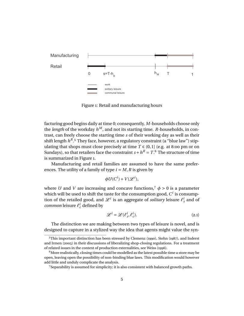
0 s=T-h h T 1

Manufacturing

Retail

RM

work

communal leisure

solitary leisure

Figure : Retail and manufacturing hours

facturing good begins daily at time 0; consequently, M-households choose onlythe length of the workday hM , and not its starting time. R-households, in con-trast, can freely choose the starting time s of their working day as well as theirshift length hR . They face, however, a regulatory constraint (a “blue law”) stip-ulating that shops must close precisely at time T ∈ (0,1] (e.g. at : pm or onSundays), so that retailers face the constraint s+hR

= T . The structure of timeis summarized in Figure .

Manufacturing and retail families are assumed to have the same prefer-ences. The utility of a family of type i = M ,R is given by

φU (C i )+V (L i ),

where U and V are increasing and concave functions, φ > 0 is a parameterwhich will be used to shift the taste for the consumption good, C i is consump-tion of the retailed good, and L

i is an aggregate of solitary leisure ℓis and of

common leisure ℓic defined by

Li=L (ℓi

s ,ℓic ). (.)

The distinction we are making between two types of leisure is novel, and isdesigned to capture in a stylized way the idea that agents might value the syn-

This important distinction has been stressed by Clemenz (), Stehn (), and Inderstand Irmen () in their discussions of liberalizing shop-closing regulations. For a treatmentof related issues in the context of production externalities, see Weiss ().

More realistically, closing times could be modelled as the latest possible time a store may beopen, leaving open the possibility of non-binding blue laws. This modification would howeveradd little and unduly complicate the analysis.

Separability is assumed for simplicity; it is also consistent with balanced growth paths.

chronization of leisure. People might enjoy differently time spent on an emptyand on a crowded beach; they might prefer going to the movies with othersthan alone. In our model, we envisage the possibility that consumers mightvalue idle time which they spend with people of their own type differently thanthe free time they spend with families of the other type. By a slight abuse oflanguage, we denote call the two types of leisure as solitary and common, withthe understanding that solitary leisure refers in our model to leisure time spentwith one’s own type, and common leisure is idle time spent with the other typeof household. In the absence of blue laws, the taste for common leisure intro-duces through preferences an externality in private consumption/leisure deci-sions.

Consistent with the balanced growth literature, we assume that

U (C ) = logC . (.)

As we will see discuss below, this specification makes labor supply in both sec-tors wage inelastic in our model. This simplification enables us to focus moresharply on the effects of leisure coordination by eliminating differences thatotherwise would stem from unequal wages across sectors. Furthermore, torule out corner solutions, we assume the usual Inada condition: V ′(0) =+∞.

The leisure aggregator function L (·, ·) is increasing and concave in each ofits arguments, and we assume that L (·, ·) exhibits constant returns to scale. Thereason for this specification is that it is required to nest within our frameworkthe standard consumption/leisure choice model, since the latter obtains in thespecial case L (ℓs ,ℓc ) = aℓs +bℓc with a,b > 0 which exhibits constant returnsto scale.

We assume that, while retail workers can shop on the job, manufacturinghousehold must shop after they stop working and before retailers close. Thisensures that M-households always choose, given T , a shift length hM

< T .

Thus the period between closing time hM in manufacturing and closing timeT in retail constitutes solitary leisure by manufacturing families. Furthermore,retail workers are assumed to be able to shop on the job. Finally, we assumethat both households face fixed costs of going to work that are large enough toguarantee that they work a solid block of time rather than disconnected shiftsthroughout the day.

The appendix briefly characterizes the elastic case.Their consumption would otherwise be zero, which cannot be optimal under our specifi-

cation for U (·) since the marginal utility of zero consumption is infinite.

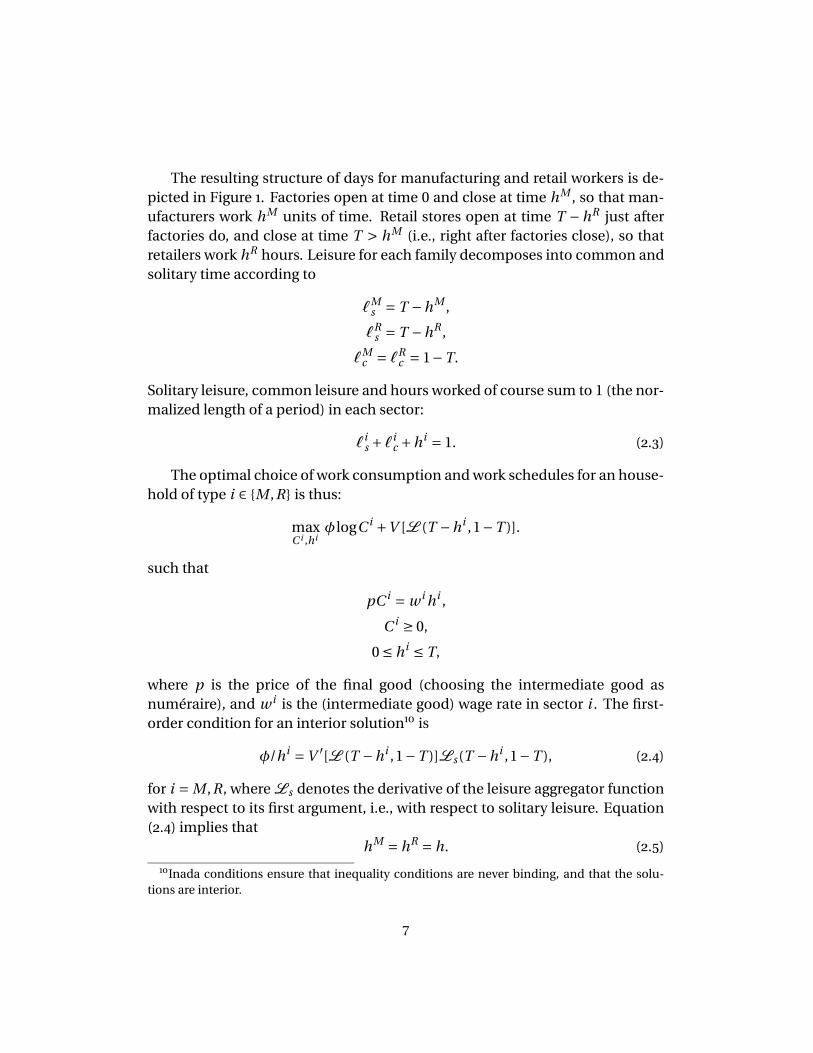
The resulting structure of days for manufacturing and retail workers is de-picted in Figure . Factories open at time 0 and close at time hM , so that man-ufacturers work hM units of time. Retail stores open at time T −hR just afterfactories do, and close at time T > hM (i.e., right after factories close), so thatretailers work hR hours. Leisure for each family decomposes into common andsolitary time according to

ℓMs = T −hM ,

ℓRs = T −hR ,

ℓMc = ℓR

c = 1−T.

Solitary leisure, common leisure and hours worked of course sum to 1 (the nor-malized length of a period) in each sector:

ℓis +ℓi

c +hi= 1. (.)

The optimal choice of work consumption and work schedules for an house-hold of type i ∈ {M ,R} is thus:

maxC i ,hi

φ logC i+V [L (T −hi ,1−T )].

such that

pC i= w i hi ,

C i≥ 0,

0 ≤ hi≤ T,

where p is the price of the final good (choosing the intermediate good asnuméraire), and w i is the (intermediate good) wage rate in sector i . The first-order condition for an interior solution is

φ/hi=V ′[L (T −hi ,1−T )]Ls(T −hi ,1−T ), (.)

for i = M ,R, where Ls denotes the derivative of the leisure aggregator functionwith respect to its first argument, i.e., with respect to solitary leisure. Equation(.) implies that

hM= hR

= h. (.)

Inada conditions ensure that inequality conditions are never binding, and that the solu-tions are interior.

The equality of optimal hours across the two sectors stems from the assump-tion that agents have the same preferences, and from restriction (.) whichensures, by making labor supply wage inelastic, that differing wages in manu-facturing and retail do not drive hours apart.

Equation (.) implies that hours h are a function of the taste parameter φand of the mandated closing time T . Given our assumptions on V and ℓ, it isstraightforward to show that a stronger taste for the consumption good alwaysleads consumers to work more. However, a relaxation in the mandated retailclosing time (a higher T ) has differing effects on hours worked depending onthe degree of substitutability between the two types of leisure in the aggregatorℓ. We postpone a discussion of these effects to the next section which exploresthe equilibrium effects of blue laws.

. Firms

We now turn to the production side of the economy, and describe how manu-facturing and retail firms operate.

.. Manufacturing

Manufacturing firms produce an intermediate (raw) good that is transformedby the retail sector into the final good consumed by our households. The man-ufacturing good Y is produced competitively with labor according to the lineartechnology

Y = hM . (.)

This linear technology implies that the wage rate in manufacturing, expressedin unit of the intermediate good, is constant and equal to 1:

w M= 1.

.. Retail

The retail good C is produced competitively by combining the manufacturinggood Y and labor according to a production function that exhibits private con-stant returns to scale in the intermediate good and hours:

C = AhR f (Y /hR ), (.)

where A > 0 is a multiplicative productivity term taken by the individual firm asgiven, and f (·) represents the production function in intensive form, with f ′

> 0and f ′′

< 0. Y can be thought of as inventories, or unpackaged and unretailedoutput. The decreasing marginal returns assumption captures the notion thatmore goods in the shops become increasingly difficult to sell without additionalmanpower, while low inventories with too many shopkeepers also result in lowlevels of service and value added per worker.

Firms maximize profits (in units of the manufacturing good numéraire)

p AhR f (Y /hR )−Y −wR hR .

The first-order condition for competitive profit maximization is thus

p A f ′(Y /hR ) = 1. (.)

Since returns to scale are constant from the point of view of the firm, and be-cause of perfect competition, the wage rate in retail is the excess of output perretail hour over factor payments to the manufacturing good input:

wR= p[A f (Y /hR )− (Y /hR ) f ′(Y /hR )]. (.)

While total factor productivity A is taken as given by individual retailingfirms, we allow for the possibility that it may depend negatively on the actionsof other agents in equilibrium via a Marshallian externality:

A = A(H R ), A′≤ 0. (.)

where H R represents the average number of hours worked in retail. We adoptthis specification in order to formalize and explore implications of the idea, ad-vanced most frequently by critics of deregulation, that longer opening hours inretail are counterproductive and attenuate productivity in that sector. Morespecifically, this externality is meant to capture “business poaching” or “ru-inous competition” which might arise from an inelastic supply of customersto the retail sector. For instance, we may think that A stands for the probabil-ity of making a successful contact with a customer. If the pool of customers isfixed but stores can vary opening hours, or more generally their search inten-sity, then A will depend negatively on the activity levels of all other retailers,holding own activity constant.

This “business-poaching” effect can be thought of as a congestion-type externality foundin matching and search models. See Diamond (), Pissarides ().

. Equilibrium

We have shown above that, because we have specified labor supply to be wageinelastic, hours are equal to h in both manufacturing and in retailing. Labormarket clearing, together with equations (.) and (.), then implies that equi-librium manufacturing output is

Y = h. (.)

Moreover, since all retail firms are identical, H R= hR in equilibrium. As

a result, using equations (.), (.) and (.), equilibrium retail output andconsumption are equal to

C = h A(h) f (1), (.)

while the equilibrium retail price and wage satisfy, from equations (.), (.),(.) and (.),

p =

1

A(h) f ′(1), (.)

wR=

f (1)− f ′(1)

f ′(1). (.)

The price of retail output thus depends negatively on hours, due to the conges-tion externality, while the retail wage rate in terms of the numeraire is constantand does not depend on the taste shifter φ or on blue laws T .

The economic effects of blue laws

In the model of the previous section, blue laws deprive consumers of choiceover the amount of communal leisure they can take. In doing so, they removethe preference-based leisure coordination externality. Our objective in this pa-per is however not to study the welfare case for blue laws or to characterizeoptimal blue laws. Instead, we wish to confront with the data the theoreticalpredictions our model makes about the effects of a relaxation of blue laws onhours, consumption and the price of the final good.

If hours were wage elastic and differed across sectors, the equilibrium p and wR would alsodepend on the input ratio Y /hR

= hM /hR which would be affected in equilibrium by a changein φ or T . The direction of this effect is ambiguous.

. Hours

We have argued in the previous section that a relaxation of the mandated retailclosing time (an increase in T ) which reduces common leisure ℓc , has differingeffects on hours worked depending on the degree of substitutability betweenthe two types of leisure in the leisure index ℓ.

Intuitively, the reduction in common leisure entailed by a postponement ofthe retail closing time induces workers to reduce solitary leisure if solitary andcommon leisure are complements. Since h = T −ℓs , this reduces hours. Bycontrast, when solitary leisure if solitary and common leisure are close substi-tutes, an increase in T , which reduces common leisure, raises solitary leisure.The magnitude of that increase depends on how valued common leisure is rel-ative to solitary leisure. If it is not very valuable, ℓs only needs to rise a little tosubstitute for the fall in ℓc , so that h = T −ℓs rises. If instead common leisureis valuable relative to solitary leisure, ℓs must rise a lot to compensate for thedecline in ℓc , so that hours h = T −ℓs rise.

To formalize this reasoning, it is useful to log-differentiate the first-ordercondition (.). This yields:

φ− h =−νL +Ls , (.)

where x ≡ d ln x/d x = d x/x denotes the log-differential of a variable x; L andLs are shorthand, respectively, for L (T −h,1−T ) and Ls(T −h,1−T ); and

ν=−

V ′′(L )L

V ′(L )> 0 (.)

is the Arrow-Pratt measure of concavity of the utility derived from the leisureindex (i.e., the elasticity of marginal utility).

The appendix establishes that constant returns to scale of the leisure aggre-gator ℓ implies that

L =λℓs + (1−λ)ℓc , (.)

while

Ls =−

1−λ

ρ(ℓs − ℓc ), (.)

where λ ∈ (0,1) is the elasticity of the leisure aggregator with respect to soli-tary leisure, and ρ > 0 denotes the elasticity of substitution between solitary andcommon leisure in the leisure aggregator.

T rises and ℓs falls.The former is a constant if L (·, ·) is Cobb-Douglas, and the latter is constant if ℓ(·, ·) is CES.

Using these two implications of constant returns to scale, we can rewrite thefirst-order condition (.) as

φ− h =−ν[λℓs + (1−λ)ℓc ]−1−λ

ρ(ℓs − ℓc ). (.)

To complete the characterization of the consumer optimum, we need tolog-differentiate the time budget constraint (.) to obtain

ℓs ℓs +ℓc ℓc +ℓhh = 0. (.)

Equations (.) and (.) constitute a system of two linear equations in twounknowns ℓs and h. Its solution depends on the taste shock φ and on changesin the blue law which can be measured directly by T or indirectly by ℓc =−(1−T )−1T . Thus, a relaxation of the blue laws, which forces retail stores to stayopen longer (T > 0), amounts to a mandated decrease in common leisure (ℓc <

0).The appendix provides a detailed solution of equations (.) and (.). It

confirms our intuition about the elasticities of solitary leisure and hours withrespect to the taste parameter and the blue law:

• Given blue laws, an increase in the taste for the consumption good alwaysreduces solitary leisure and raises hours: ∂ℓs/∂φ< 0 and ∂h/∂φ> 0 for allparameter values.

• When the elasticity of substitution between solitary and common leisureis low, a decrease in common leisure lowers solitary leisure and raiseshours: ∂ℓs/∂T < 0 and ∂h/∂T > 0 when ρ is close to zero.

• When the elasticity of substitution between solitary and common leisureis high, a reduction in common leisure raises solitary leisure: ∂ℓs/∂T > 0when ρ→+∞. The effect on hours depends, however, on λ, the elasticityof the leisure aggregator with respect to solitary leisure which measureshow valuable solitary leisure is (or, equivalently since ℓ exhibits constantreturns to scale, how little consumers care about common leisure):

– When common leisure is not very valuable to consumers relative tosolitary leisure (λ large), ℓs rises little to substitute for the fall in ℓc ,so that hours rise: ∂h/∂T > 0 when ρ→+∞ and λ→ 1.

– When common leisure is very valuable to consumers relative to soli-tary leisure (λ small), ℓs rises a lot to substitute for the fall in ℓc , sothat hours fall: ∂h/∂T < 0 when ρ→+∞ and λ→ 0.

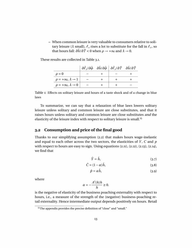
These results are collected in Table ..

∂ℓs/∂φ ∂h/∂φ ∂ℓs/∂T ∂h/∂T

ρ = 0 − + − +

ρ =+∞, λ→ 1 − + + +

ρ =+∞, λ→ 0 − + + −

Table : Effects on solitary leisure and hours of a taste shock and of a change in blue

laws

To summarize, we can say that a relaxation of blue laws lowers solitaryleisure unless solitary and common leisure are close substitutes, and that itraises hours unless solitary and common leisure are close substitutes and theelasticity of the leisure index with respect to solitary leisure is small.

. Consumption and price of the final good

Thanks to our simplifying assumption (.) that makes hours wage-inelasticand equal to each other across the two sectors, the elasticities of Y , C and pwith respect to hours are easy to sign. Using equations (.), (.), (.), (.),we find that

Y = h, (.)

C = (1−α)h, (.)

p =αh, (.)

where

α=−

A′(h)h

h≥ 0.

is the negative of elasticity of the business poaching externality with respect tohours, i.e., a measure of the strength of the (negative) business-poaching re-tail externality. Hence intermediate output depends positively on hours. Retail

The appendix provides the precise definition of “close” and “small.”

output moves with hours only if the “business poaching” externality is not toostrong (α< 1), while the price of retail goods rises or falls together with hours aslong as α> 0. In a more general model in the absence of externalities, the effecton regulation is likely to increase retail prices relative to the market allocation,which is always Pareto optimal.

Combining these results with those of the previous subsection, we concludethat, unless solitary and common leisure are close substitutes and the elasticityof the leisure index with respect to solitary leisure is small, a relaxation of bluelaws raises intermediate output and has the following effects:

• It raises final output consumption if the business poaching externality isnot too big.

• It increases the price of final output if there is a business poaching ex-ternality, with the magnitude of the effect depending positively of thestrength of the externality;

These results are important when contrasted to the public policy debateon shop-closing regulations. Stützel (, ) claimed that retail openinghours regulations do not have first-order effects on the real demand for finalgoods, because consumers respond to restrictions on shopping hours by sim-ply concentrating the purchases in a shorter time interval. This argument isfrequently advanced by trade unions and small shop owners to resist liberal-ization of shopping hours regulations. Equation (.) shows that “Stützel’s Para-dox” does not in general hold in our model. In point of fact, unless solitary andcommon leisure are close substitutes and the elasticity of the leisure index withrespect to solitary leisure is small, a relaxation of blue laws boosts retail outputeven in the presence of a small (but moderate) productivity externality.

It is interesting to note that recent surveys in Germany, Switzerland and Italy have revealedfears among consumers that deregulation of the currently severe shop closing regimes (by USstandards) would lead to price increases, which is consistent with the existence of a negativeretailer externality. See Ifo-Institut (, ).

These predictions can be compared with those of Gradus (), who studies a more con-ventional demand/supply framework with increasing returns at the firm level. He predicts adecrease in retail prices and margins resulting from regulation, as well as an increase in sales,and an ambiguous effect on employment. However, in his model, the socially optimal policy is hours (round the clock opening hours), which suggests that his model does not consider allgeneral equilibrium channels.

. The economic rationale for blue laws

Why would governments implement blue laws? Until now, we have sidesteppedthat question, primarily because we are more interested in the empirical ef-fects of blue laws on observable economic outcomes. The existence of shopclosing regulations might reflect lobbying efforts by retailers or trade unionists,or other groups interested in issues of coordination. They may even originatefor reasons which have little to do with the issues addressed in this paper. Inthis section we briefly characterize the optimum as seen from the perspectiveof a social planner who can explicitly account for consumption and produc-tion externalities assumed in the model. If private markets are unable to attainthis allocation for reasons of transactions or coordination costs, or if markets inshared leisure are ruled out, then blue laws might be seen as a second or thirdbest solution to the problem of societal coordination.

In the appendix, we sketch the social optimum in our economy, which issimply the solution to a maximization of the unweighted sum of the two house-holds’ utilities subject to the given resource constraints. Comparison of first or-der conditions for the planner and the decentralized market in the absence ofblue laws (T = 1) shows that the market replicates the planner’s optimum onlyby chance. One case is when γ= 0 and if T is chosen such that V M

2 =V M3 . Even

if it were in R-family’s interest to induce this outcome strategically, sufficient in-struments are generally unavailable to do so. Evidently, the failure of the marketto achieve the social optimum lies in the fact that conditions necessary for thefirst and second welfare theorems do not obtain. Communal leisure is a non-rival “good“ which is not traded in a market, presumably due to the difficulty inassigning property rights. Just as in the vision of Marshall, infinitesimally smalltraders do not internalize the congestion externality they inflict on each other.

One could imagine a number of institutions – clubs, religion and slavery forexample – which could solve the coordination problem at some level for somegroup of agents. Retailer’s associations, shopping malls and Wall-Marts mightbe thought of as attempts to solve the Marshallian externality. To the extentthat Pigovian taxes are unavailable, a shop closing regulation can be seen asan attempt for the state to move the economy towards more shared leisure orrestrained competition; it should be noted however, that one instrument willgenerally be inferior in achieving the planner’s objectives. To the extent that

Because the two representative families are thought of as stand-ins for an infinitely large setof atomistically small families, simple side payments will not be feasible. Some form of societalcoordination will be necessary.

coordination was undersupplied in the first place, blue laws achieve the firstbest only when γ = 0. More generally, when γ > 0, we are in a second bestworld, and the blue law regulation T will be insufficient for dealing with twodifferent market failures.

Evidence for economic effects of blue laws in US

states

. Empirical Strategy: An Overview

In this section, we entertain the hypothesis that restrictions on retail activity– here in the form of Sunday closing or ”blue laws” – have an effect on em-ployment, wages, retail prices, and other variables, and use data from the USstates to test those implications. The model elaborated in the preceding sec-tions allows us to identify qualitative predictions for the effects of blue laws onobservable variables. Under assumptions of separability of utility with respectto consumption and unit elasticity of utility with respect to consumption, theeffect of a deregulation (T > 0) can be summarized as follows:

• The strength of the common leisure externality determines the directionof the net effect of blue laws deregulation on employment.

• If the elasticity of substitution between solitary and common leisure (ρ)is low, a deregulation raises employment unambiguously.

• If the elasticity of substitution between solitary and common leisure (ρ) ishigh, the effect of deregulation will depend on how much the householdvalues solitary leisure given its overall valuation of leisure in utility (λ). Ifthis valuation is high - put differently, the valuation of common leisure islow - , hours rise in response to a deregulation; if it is low however, hourscan actually decline.

• The existence of the Marshallian congestion effect, summarized by γ, canbe tested by the reaction of retail price to employment. Since the modelin the text rules out income effects, employment and the price of valueadded in retail will move in the same direction. Note that in the standardmodel without externalities, retail prices are likely to rise in response toregulation.

• The real wage will move in the opposite direction to employment.

• Stützel’s Paradox - meaning that the volume of consumption is constantdespite a deregulation of opening hours - obtains on a set of measurezero. To the extent that hours increase, the relative price of retail shouldbe higher, meaning deregulated regimes will exhibit higher retail prices.

We now investigate these hypotheses from several different perspectiveson a number of data sets. Rather than specifying and estimating a struc-tural model, we focus on nonparametric, fixed-effect models (”difference-in-difference”) specifications which attribute all other temporal influences to asingle, common trend. The discussion of the last section suggests, however,that it may be necessary to take the issue of endogeneity of regime seriouslywhen attempting to identify the effects of the laws in aggregate date, sinceauthorities acting in the public interest are likely to implement regulations inthose regions in which the gain from harmonizing leisure are greatest. This willnecessitate a careful search for instruments, which can be guided by the predic-tions of the model. Finally, we examine the influence of blue laws on individuallabor market outcomes using the CPS (Current Population Survey of the US) toverify the effects of the model at the individual level.

. Blue Laws in the United States

The central element of the empirical analysis is a unique dataset of blue lawsregulation in the US states for the period -. The collection of thesedata involved a tedious review of state legislative records to identify and trackchanges in regulatory regimes. Because it is difficult to accommodate everynuance in state legislation, a set of eight dummy variables were defined overthe sample. Most important among these are the dummy variables SEV (se-vere), MOD (moderate) and MILD, which describe the law in place during theyear in a particular state. SEV describes a state regime in which Sunday sales isseverely regulated, with exemptions represent exceptions rather than the rule.Trade in food, tobacco, liquor as well as hardware, clothing and other goods areprohibited. MOD refers to regimes which exempt food explicitly from the SEV

The period for analysis stops in , to avoid complications that arise from the growing useof internet in retail activity.

Descriptive statistics of these variables can be found in the Appendix.

regime, while MLD adds a number of additional exceptions to food, includ-ing hardware, dry goods, or appliances, but continue to rule out trade in someproducts, especially alcoholic beverages. These dummy variables are definedincrementally, so all state-years with a value of for MOD also take the value of for MLD, etc. An extended set of additional laws were encoded for the analysisconsists of states with Sunday prohibition of motor vehicle sales (MVR), Sun-day closing regulations applying solely to large establishments (LBS), commonlabor restrictions prohibiting hiring on Sundays (CLR), and devolution of au-thority to regulate Sunday trading to local communities (LOC). Descriptives ofthese variables are displayed in Table .

In the complete sample of fifty US states (Washington DC was excluded)over the period -, .% of the state-year observations had some formof blue law on the books in the narrow sense, meaning either SEV, MOD or MLDequaling one; this rises considerably if one includes restrictions on motor vehi-cle sales (MVR: .% of all observations), devolution of regulatory discretion tolocal authorities (LOC: .% of all observations), limitation on large retail busi-nesses (LGB: .%) and common labor restrictions (CLR: .%). The last regula-tion is particularly interesting because it survives in some European countries(e.g. France) Both time and cross-sectional variation is clearly evident in thedata. An analysis of variance shows that while the legal variables do indeed ex-hibit some time variation, more than % of the total variance of the dummyvariables is due to between-state differences. At the same time, heterogeneityamong states within regions and over time appears to be significant, for exam-ple, in Vermont, Florida, Washington, Arkansas and Tennessee.

. Macroeconomic Evidence from the US states

In this section we examine the impact of blue laws on observable outcomes:employment, compensation, productivity, prices and related variables in a bal-anced panel of US states.

.. Data

A primary source of US state level aggregate data is the Regional Economic In-formation Service (REIS) of the Bureau of Economic Analysis, U.S. Departmentof Commerce. Also known as the Regional Economic Accounts, this data setconsists of annual observations of US states of annual full and part-time em-ployment, aggregate annual compensation of full and part time employment

and salaried employees, sectoral nominal and real value-added, and other vari-ables. These data were available for the SIC classification (retail trade in thebroad sense), while employment and total compensation per employee werealso available for at the three-digit level of sectoral disaggregation .The data areavailable respectively from - (employment and compensation) or - (REIS value added data). Subject to data availability, we construct a panelof the fifty US states over the period extending from -. Because manyvariables are available for only a subsample of this period or only sporadically,however, the estimation period will generally be shorter. Summary statisticsof the data used is presented in Table for the entire sample as well as thosestate-years with a value of for MLD, MOD, or SEV.

A second source of data used in studying the effects of blue laws on labormarkets involves the US Current Population Survey (CPS), the national labormarket survey which serves as the basis for the most important official US laborforce statistic measures. For outgoing March rotation groups in the period -, we constructed the following data generated by running state counts onCPS data and constructing the following estimates for each state i and year t :

• the proportion of all workers employed in retail (SIC , or in therevised enumeration)

• the proportion of all workers in part-time employment (self-reported, de-fined as less than x hours weekly)

• the proportion of all employed workers in both retail (SIC , in therevised enumeration) and part time

• the proportion of all employed workers employed in department storesand mail order business.

• the nominal hourly wage, in retail and in the overall economy.

Since these variables are used in the empirical analysis solely as regres-sands, sampling error is an issue of estimation efficiency, but not consistency.

.. An econometric model of the effects of blue laws: OLS estimates

We will consider the following reduced form statistical relationship implied bythe theoretical model, which determines the outcome of some variable of in-terest y in state i in sector j and in year t , yi j t , is given by the following linear

reduced form model:yi j t = a′xi j t +b′Ti t +εi j t (.)

where Ti t stands for a vector of blue law dummy variables, a and b denote co-efficient vectors, and xi j t is the value taken by state i for variable x in year t .Constants are suppressed for simplicity.

The first step in the empirical analysis consists of OLS estimates of (.) forFPT employment, FPT compensation, value added per FPT employed, value-added share, as well as labor market indicators extracted from the CPI. Employ-ment variables are expressed as natural logarithms of the fraction of the totalstate population. This normalization was preferred to one relative to an esti-mate of labor force or working age population for two reasons. First, consistentlabor force data from individual states are unavailable before the mid-s;second, a participation estimate based on working age population may neglectfull and part-time employment of teenagers and statutory retirees. The vectorx consists of time and regional fixed effects, which effectively means that analy-sis attributes deviations of state realizations of the variables of interest from theregional and temporal averages to the blue laws. As noted above, within statevariance is a modest component of total variance. Each line in the table repre-sents a single OLS regression of the variable of interest, where T is a compositedummy variable (BLUE) which takes the value if any of the blue law regimes isin place. The spatial nature of the data set and the differing proximity of statesimplies potential neighboring state effects. We control for these effects by con-structing a dummy BLUEREL, a weighted average of the simple blue law regimemeasure in contiguous states, using each state’s individual share in the totalborder with contiguous US states. Robust (that is, White-heteroskedasticityconsistent) standard errors are reported. To save space, we report only esti-mated coefficients and significance levels, as well as the F-statistic that all co-efficients on the blue law variables are jointly zero.

The first two columns of Table present the first set of empirical re-sults for the impact of blue laws on ”macro” US state FPT employment andsalary/compensation data. For full and part time salaried FPT employment,the results are uniform and negative, with the exception the apparel sector, withthe presence of a blue law restricting Sunday trade having between -. and -. log points on the log fraction of the population employed as a salary work-ers in three digit sectors. Blue laws are also negatively associated with overallsalaried employment, which is consistent with our theoretical model as well asa broader measure which includes the self-employed. Evaluated at the overall

sample mean for the fraction of state population in salaried FPT non-food re-tail employment (.%), the point estimate for overall non-food retail (-.)implies an average effect of . percentage points of the population, or about, jobs in the average US state over the period. The overall effect for salariedemployment (.% of the population) implied by our point estimate (-.)is .% or about , jobs per state. Blue laws are positively, albeit weakly,associated with wage outcomes in the same sectors, where the wage is mea-sured as annual compensation, less so when measured as retail hourly wagerelative to the state average. For non-food retail, the existence of a blue lawis associated with . log points lower annual compensation, measured rela-tive to average state compensation per FPE overall. This translates at samplemeans to .% less annual compensation relative to the state average, or about$ annually.

Table also presents estimated effects of blue laws on other GSP variablesfor the retail sector as well as the state retail variables estimated using the CPS.A central implication of the model, which discriminates it from a conventionalmarket economy in which the welfare theorems hold, is the effect of blue lawson the price of retail (the price of value added in the retail sector). The resultspresented in Table show a weak and negative association of Sunday closingwith retail prices. The price effect ranges to -. to -. log points, althoughthese are not always statistically significant. Blue laws are significantly asso-ciated with lower productivity and the share of value added in total state GSP(insignificantly). The OLS estimates on CPS data reveal that the blue law is as-sociated with . percentage points lower employment in retail (measured asa fraction of overall CPS employment) as well as in . percentage points lowerpart-time. Given the respective percentages in the sample (.% and .%),these are very large effects. It is interesting to note that while we estimate a sig-nificant relative wage hourly wage effect on retail, we do not estimate an overallreal wage effect.

.. Differentiated measures of blue laws

In Tables and we present estimates using more differentiated measures ofblue law regulations. The results are not qualitatively different from the simpleones, although it appears that the degree of severity of the law affects our vari-ables of interest in a nonlinear and possibly a non-monotonic fashion. For FPTemployment, the effect of the law in the mild form (MLD) is negative for theapparel sector, while the miscellaneous group is negative but not statistically

significant at conventional levels. For the MLD regime which allows trade infood and some other product, a significant impacts ranging from -. to -.

log points were estimated. In three three-digit sectors, a positive coefficienton MOD implies that a more extensive prohibition (except food) undoes somebut not all of this effect; for the others the negative effect is actually intensified.Only in home furnishings are we not able to reject the irrelevance of blue lawsfor employment.

For compensation, the differentiated treatment of blue laws strengthens thecase that relative compensation is higher in mild regimes. This is undone tosome extent as the law reaches maximal severity. Indeed, the sum of the pointestimates for MLD, MOD, and SEV is positive with only two exceptions (,building materials and garden equipment and , food and grocery stores).For the price variables, the effect of MLD is positive, more than offset by MOD,but then neutralized by the severe regime; this pattern holds for two indepen-dent sources of data (the GSP deflator for retail and a weighted average of SMSAconsumer price indexes constructed by Marco Del Negro). Overall, we cannotreject the hypothesis that the laws are neutral with respect to retail prices. Ourfindings for the CPI state aggregate data are consistent with those for the simpleblue law indicator, yet these effects appear to be highly nonlinear.

.. Endogeneity of Blue Laws and Instrumental Variable Estimation

Because a trend towards deregulation is evident in many states and becausesystematic differences exists between and within US regions, it is probably in-appropriate to assume an exogenous regulatory environment in the economet-ric estimation. While we eschewed an explicit welfare analysis, we argued in-formally that blue laws could represent the optimal choice of agents. In par-ticular, differing tastes for consumption φi , differing preferences for coordina-tion of leisure ρ or λ, or strong Marshallian effects in retail γ (perhaps becausethe business stealing effect is strong) could give rise to regulation restrictingopening hours. The problem is a common one: in democracies, public institu-tions, including regulatory regimes, tend to reflect the popular will, which canvary over time and space. In a panel context, endogeneity of policy may neveremerge over time, but could still be reflected between units in the data set; thepredominance of variance between states in the blue law dataset alerts us tothis potential problem. If blue laws are indeed endogenous, OLS estimates willsuffer from simultaneous equation bias.

To see this, suppose that the model is now

yi j t = a′xi j t +b′Ti t +ui j t +εi j t (.)

where ui j t is an unobservable taste variable. Blue laws themselves are deter-mined by

Ti j t = c ′xi j t +d ′zi t +eui j t (.)

where xt and zt represent factors which motivate state legislatures to pass bluelaws, and c and d are coefficient vectors. Because the vector xi j t appears inequation (.) as well, only zt , the excluded determinants of T , allow us to iden-tify statistically the elements of b. Most important of these factors is the ”taste”for retail, which was represented in the model as φ, which determines the mar-ginal utility of consumption. States with high values of φ (strong preferencesfor consumption) or are indifferent towards communal leisure or preferencesfor shopping while others are working, should be less likely to have blue laws(e < 0). Since tastes are unobservable, an econometrician estimating (.) usingOLS will necessarily include tastes in the error term, leading it to be correlatedwith T . If b < 0, estimates of it will be positively biased.

Our ability to estimate the effect of blue laws consistently will thus dependon the availability of instruments, that is, variables z which are correlated with,or causal for T but also orthogonal to u, i.e., uncorrelated with household tastesfor leisure and consumption? In effect, we seek factors which have led to the in-stitution of blue laws which are independent of direct impact on retail variablespredicted by the model. In particular, our strategy will be to isolate factors as-sociated with the existence of blue laws which are nevertheless independent ofthe determinants of retail outcomes, as predicted by mechanisms described inthe paper. These will tend to be those factors which limit a state’s ability to im-plement retail restrictions, or its desire to coordinate household activity, evenif its inhabitants would want these restrictions. From this perspective we con-sidered the following candidates for instruments:

• the log of state land area

• the log of state population

• urban density

• the fraction of Democrats in the state legislature (as fraction of the sumof Democrats and Republicans)

• weighted influence of adjacent states’ regimes, with weight adapted for”average distance to the border”

• religious affiliation, summarized by the US Census decennial survey ofChristian adherents.

The rationale for these instruments is as follows. Geographically vast statestend to be ethnically more diverse, suggesting less demand for coordinationand common leisure (who in southern California cares what northern Califor-nians are doing); at the same time, larger states present more difficulties in co-ordinating individual’s schedules as well. Holding land mass constant, morepopulated states will have more potential interactions (by sheer nature of thecombinatorics) and should exhibit greater demand.for leisure coordination, ce-teris paribus. Urban density (fraction of population living in urban areas) re-flects the expectation that cities are areas of more intense economic activitywith individuals who have a high valuation of their leisure time and thus needto shop on Sundays. The fraction of Democrats represents ”pro-labor” views,which are generally associated with ”more humane” work schedules. The in-fluence of regimes from neighboring states represents a restriction on a givenstates ability to conduct an independent blue law policy. Finally, Christian pop-ulation represents the demand for the blue law in order to enforce the Sabbathon Sundays.

The first stage regressions for the instruments are presented in the appen-dix. Without exception, the instruments have the sign we predict in the discus-sion above. Taken together with the fixed effects, the instruments are capable of”explaining” about % of the state-year variation in the simple blue law vari-able. Table presents IV estimates for simple models estimated by OLS in Table. These results are qualitatively consistent with the results presented above,but do not exhibit the same degree of statistical significance Employment issignificantly affected by blue laws, while wages and prices are not. The point es-timates for the effects on employment are from three to ten times larger than inthe OLS case. Productivity is negatively effected, which signals that economicefficiency is attenuated by regulations. The ”Marshallian” mechanism providedby our model is not supported by the evidence.

In Europe, labor unions actively defend not only Sunday closing but also end of day closing- for example in the shop closing law in German (Ladenschlußgesetz) requires store toclose after : pm as well as Sundays and public holidays, with only minor exceptions.

This is due to the use of IV estimation as well as robust standard error estimates which areclustered by US state.

. Microeconometric Evidence

.. Data

To provide some further independent validation of the effects we isolate, weemploy directly information contained in the CPS March rotation groups in theperiod -. By merging blue laws data with information on employed in-dividuals (including state of residence), it is possible to estimate the impact ofblue laws in reduced forms in which the individual observation is an individualin the CPS. The individual CPS data can thus provides ”independent” verifica-tion of the macro US state results.

For the pooled sample consisting of all March files from -, we con-sidered the following variables on individual workers in employment : () lognominal and () real weekly gross earnings, () log weekly hours () log nom-inal and () real hourly wages. We dropped all workers earning less than $

or more than $ per hour. In a standard ”Mincer-style” specification used forearnings equations, we regressed the log of the dependent variable on potentialexperience, its square, education in years and its square, sex, sex interactionswith all of the aforementioned covariates, sectoral dummies, occupationaldummies, and the regional and national time fixed effects. The blue laws wereincluded as the levels of the three state blue law variables MLD, MOD and SEV,plus an interaction of these three with affiliation with the retail sector - definedwithout eating and drinking establishments.

.. Results

The results support the conclusion that Sunday closing regulation affects la-bor market outcomes negatively. While the level effects of the dummies arerarely significant, they are strong and significant in their interaction with theblue laws. For example, we estimate that a retail worker in a SEV regime stateearns about log points less per week than a comparable worker in a state with-out any blue laws. As with the macro data, there appears to be a nonlinear ef-fect, with the effect initially negative, then less so, then finally strongly negative(the sum is frequently significantly different from zero at the .% level of sig-nificance). Workers in a SEV regime in retail work about half-an hour less thanin unregulated states. The net real wage effect is positive and significant, at .log points - although it decreases with the milder regimes and increases sharplyin the SEV regime. This is consistent with the macro results if the net effect ofblue laws is to concentrate employment in the form of full time employees, who

receive more lump sum compensation than their equivalent in part-time work-ers. The net result is to increase compensation per FPT employee, even whilehours and employment are declining.

. Summary of Results and Relation to Previous Work

The preponderance of the aggregative and individual evidence indicates thatblue laws have a significant negative effect on employment but a milder, am-biguous effect on relative and real wages. This is more strongly borne out bythe microeconometric evidence, which indicates that earnings are lower, ce-teris paribus, in blue law states but especially for those individuals working inthe narrowly defined retail sector. The effect appears to arise primarily from anegative effect on hours, but also real wages.

While the evidence for the evolution of full and especially part-time em-ployment appears incontrovertible, there is little robust evidence that shop-closing regulations reduces prices in US states, measured as the relative pricedeflator of retail sector output relative to overall state value-added. Our modelwould have allowed for this, and would also have predicted a negative effect ofblue laws on prices as long as inefficient business-stealing was curtailed in theprocess. Even if they did reduce prices, however, it would not be clear that theydid for reasons suggested by our model. Thus the evidence for the first type ofexternality survives, while second one finds little support. This stands in con-trast to existing research in this area: Tanguay et al. () find that prices in-creased at large department stores after deregulation in Quebec. Recent discus-sion of liberalization in Europe is accompanied by consumer fears that dereg-ulation will be associated with price increases.

While the theoretical literature on retail trading restrictions address a vari-ety of important issues, they have generally ignored macroeconomic, generalequilibrium effects on product and especially labor markets. Most work hasfocused on the effect of shop trading laws on retail industrial organization, orthe search-theoretic aspects of uniform closing times. De Meza () showsthat, in the Salop model with imperfect competition, shop regulation can ac-

A second interpretation is that retail’s contribution to national value-added is mismea-sured. If the quality of retail output improves over time, fixed current weight deflators willoverestimate price and underestimate quality changes. To the extent that regulation retardsimprovements in retail service quality and lower price changes are measured, regulation willbe ”credited” with keeping prices in stores down, although the quality of retail output will beinferior.

tually induce more competition and result in lower travel costs as well as lowerprices. In contrast, Clemenz () concludes that deregulation is associatedwith more search, better price information, while leading possibly to highershopping costs. Tanguay et al. () study the reaction of prices to shoppinghours liberalization when smaller stores are closer, but larger, cheaper storesare farther away. Morrison and Newman () show that smaller, inefficientfirms have the most to gain from retail operation restrictions. In a spirit similarto our model below, Bennett () provides an analysis of the peak load aspectsof shop opening times, invoking arguments by Becker (). Gradus ()studies the effects of shop liberalization using a partial equilibrium supply-demand model with parameters estimated from a Swedish study.

Conclusion

A fundamental problem in a society whose members value shared or commu-nal leisure is how to coordinate activity. Even with an explicit assignmentof property rights, it would be difficult to imagine trade in coordinated, sharedleisure. Yet mechanisms exist which could move an economy towards first-best;country clubs, athletic associations, traditional siestas, organized mass specta-tor sports and religion all represent potential vehicles of leisure synchroniza-tion. Yet in heterogeneous societies with widely different marginal valuationsof leisure and consumption, these mechanisms may not be sufficient; moralor ethical inducements such as religion might be more cost-effective. The so-cial value of religion will depend on the extent that leisure is coordinated, withlikely ”superstar” effects. In that sense, it may matter less whether the Sabbathis Friday, Saturday or Sunday, as long as we mostly agree that there is one, andkeep it.

While this concern appears less pronounced in the United States, it is an important elementof the European policy discussion. For example, in their extensive survey of shop-closing regu-lations, the Ifo-Institute paid particular attention to public opinion surveys placing more valueon ”social” free time on Saturdays compared to weekday evenings (Ifo-Institute : -).

Among other things, this may explain why the service sector is more developed in ethnicallyheterogenous economies (the US, Canada, UK) compared with more homogeneous societiesof northern Europe and Scandinavia.

Besides the public interest approach, the more cynical ”political economy” view of shopclosing laws would attribute regulation to special interest lobbying and regulatory capture. Ourstudy has distanced itself from this idea but our empirical results can be interpreted as showingthe consequences which can be expected from deregulation. For an interesting contribution to

The empirical evidence suggests however, that shop closing regulationsmay be a high price to pay for societal coordination, especially as the shadowvalue of time rises over time and makes search increasingly costly. The largeand significant effects on employment we estimate must be put be comparedwith any putative gains from synchronized leisure. European countries cur-rently debating the merits of deregulation of both product and labor marketderegulation should be consider significant increase in flexible employmentcreation linked to deregulated retailing. It is not coincidental that the retail sec-tor has the largest fraction of part-time workers in the US, and that the Nether-lands has enjoyed high growth in retail (especially part-time jobs) since dereg-ulating shop closing in the mid-s.

To our knowledge, this paper provides the first comprehensive analysis ofthe effects of blue laws on labor market outcomes in the United States. It shouldhowever be stressed that our results - while applicable to a retail sector in whichalmost a fifth of all workers is employed – can be applied to any service whichinhibits joint leisure on the part of agents, including travel agency, banking andinsurance brokerage, personal and health care services. The coordination of ac-tivity is a fundamental aspect of services, which now dominate growth in jobsand economic activity in most advanced economies of the world: some mustwork while others consume, enjoy leisure, or both. In a richer model, the prob-lem is likely to be aggravated by complementarities in utility between the two.

References

Batzer, E. () “Änderung des Ladenschlußgesetzes“? Ifo-Schnelldienst /,-.

Becker, G. () “A Theory of the Allocation of Time“ Economic Journal:-.

Bennett, R. () “Regulation of Services: Retail Trading Hours,“ in B.Twohill, ed., Government Regulation of Industry Conference Series Number ,Newcastle: Institute of Industrial Economics.

Clemenz, G. () “Non-sequential Consumer Search and the Conse-quences of a Deregulation of Trading Hours,“ European Economic Review:-.

De Meza, D. () “Is the Fourth Commandment Pareto Optimal“? Eco-nomic Journal : -.

this dimension of shop-closing regulation, see Thum and Weichenrieder ().

Euromonitor () (ed.) Retail Trade International Vol. - London.Gradus, R. () “The Economic Effects of Extending Shop Opening Hours“

Journal of Economics :-.Hamermesh, D. () Workdays, Workhours and Work Schedules, Kalama-

zoo: Upjohn Institute for Employment Research.Holmes, T. () ”The Effects of State Policies on the Location of Manu-

facturing: Evidence from the State Borders,” Journal of Political Economy :-.

Ifo-Institut für Wirtschaftsforschung () Überprüfung des Laden-schlußgesetztes vor dem Hintergrund der Erfahrungen im In- und Ausland (Anassessment of shop-closing regulation in the context of domestic and interna-tional experience). Report to the Federal Labor and Economics Ministries, Mu-nich, August.

Imgene, C. () “The Effect of ’Blue Laws’ on Consumer Expenditures atRetail,“ Journal of Macromarketing :-.

Inderst, R. and A.Irmen () ”Shopping Hours and Price Competition ”European Economic Review : -.

Kay, J. and C. Morris () “The Economic Efficiency of Sunday Trading Re-strictions,“ Journal of Industrial Economics :-.

Kay, J., C. Morris, S. Jaffer, and S. Meadowcroft () The Effects of Sun-day Trading:The Regulation of Retail Trading Hours. London: Institute of FiscalStudies Report Series No..

Knott, A. () Das Ladenschlußgesetz. Mögliche Auswirkungen einer Liber-alisierung auf den Einzelhandelssektor. Diplom-Thesis, Humboldt-Universitätzu Berlin.

Laband, D. and D. Heinbuch () Blue Laws: The History, Economics, andPolitics of Sunday-Closing Laws Lexington: Lexington Books.

Levitt, S. and J. Synder () ”The Impact of Federal Spending on HouseElection Outcomes,” Journal of Political Economy , -.

Morrison, S. and R. Newman () “Hours of Operation Restrictions andCompetition Among Retail Firms,“ Economic Inquiry :-.

Putnam, R. () ”Bowling Alone: America’s Declining Social Capital” Jour-nal of Democracy : -.

Rybczynski, W. () “Waiting for the Weekend,“ The Atlantic Monthly Au-gust.

Sanyal, K. and R. Jones () “The Theory of Trade in Middle Products,“American Economic Review .

SOU () Betänkande av års affarstidsutredning Affärstiderna :

Stehn, J. () “Das Ladenschlußgesetz – Ladenhüter des Einzelhandels“?Kieler Discussion Paper No. , January.

Stützel, W. () Volkswirtschaftliche Saldenmechanik: Ein Beitrag zurGeldtheorie. Tübingen: J.C.B. Mohr.

Tanguay, G. L. Vallée, and P. Lanoie () “Shopping Hours and Price Lev-els in the Retailing Industry: A Theoretical and Empirical Analysis,“ EconomicInquiry :-.

Thum, M. and A. Weichenrieder () “‘Dinkies’ and Housewives: The Reg-ulation of Shopping Hours,“ KYKLOS Vol. ():-.

Weiss, Y. () “Synchronization of Work Schedules,“ International Eco-nomic Review :-.

Appendix A Log-differentiation of model

This appendix shows how to log-differentiate the solitary/common leisuremodel of section .

A. Computation of L

Since L =L (ℓs ,ℓc ),

L =

Lsℓs

Lℓs +

Lcℓc

Lℓc .

Since the aggregator function L (ℓs ,ℓc ) exhibits constant returns to scale,

Lsℓs +Lcℓc =L , (A.)

so that if we define

λ=

Lsℓs

L,

with λ ∈ (0,1) because of property (A.) and the assumption that Li > 0, wehave

L =λℓs + (1−λ)ℓc , (A.)

which establishes equation (.) in the text.

A. Computation of Ls

Log-differentiating equation (A.) yields

λ(Ls + ℓs)+ (1−λ)(Lc + ℓc ) = L .

Using equation (A.) to eliminate L , this implies that

Ls = (1−λ)(Ls −Lc ).

Now the elasticity of substitution between solitary and common leisure in theaggregator function L (ℓs ,ℓc ) is, by definition,

ρ =−

ℓs − ℓc

Ls −Lc

> 0.

As a result, we conclude that

Ls =−

1−λ

ρ(ℓs − ℓc ), (A.)

which is equation (.) in the text.

A. Computation of ℓs and h

Equations (.) and (.) can be written in matrix form:(

θs −1

ℓs ℓh

)(

ℓs

h

)(

θc ℓc − φ

−ℓc ℓc

)

, (A.)

where

θs =λν+ (1−λ)/ρ > 0, (A.)

θc = (1−λ)(1/ρ−ν) = θs −ν. (A.)

The determinant of the matrix on the lefthand side of (A.) is

∆= θsℓh +ℓs > 0.

The solution of (A.) is

ℓs∆−1[(θcℓh −ℓc )ℓc −ℓhφ],

h∆−1[−(θsℓc +θcℓs)ℓc +ℓsφ].

The elasticities of solitary leisure and hours with respect to the taste shifterand solitary leisure are thus

∂(ℓs , h)

∂(φ, ℓc )=∆

−1

(

−ℓh ℓs

θcℓh −ℓc −(θsℓc +θcℓs)

)

= M .

M11 < 0 and M12 < 0 for all parameter values. Using the definition of θc andθs above, it is trivial to show that M21 > 0 if and only if

ρ <

(

ν+1

1−λ

ℓc

ℓh

)

−1

,

while M22 < 0 if and only if

θs =λν+ (1−λ)(1/ρ) > νℓs

ℓs +ℓc. (A.)

As ρ→∞, the last inequality is equivalent toλ> ℓs/(ℓs+ℓc ). For givenλ ∈ (0,1),inequality (A.) is always satisfied if ρ is close to 0.

These computations justify the characterization of the elasticities of solitaryleisure and hours with respect to the taste shock and common leisure given insubsection ..

Table 1. Summary statistics on variables employed Variable, Sector All observations Blue law observations

Mean Std.dev Max Min Mean Std.dev Max Min Employment (fraction of state population)All FPT employment 0.5090 0.0579 0.6631 0.3721 0.4963 0.0581 0.6594 0.3721

620 Total SIC retail 0.0820 0.0130 0.1197 0.0450 0.0784 0.0140 0.1197 0.0502

All FPT salary employees 0.4259 0.0497 0.5623 0.3077 0.4183 0.0495 0.5402 0.3077

620 Total SIC retail 0.0704 0.0123 0.1072 0.0385 0.0672 0.0132 0.1072 0.0389

620 Total SIC retail less 627 0.0490 0.0065 0.0755 0.0294 0.0483 0.0073 0.0755 0.0324 621 Building materials, garden equip. 0.0032 0.0009 0.0081 0.0006 0.0031 0.0010 0.0081 0.0016 622 General merchandise stores 0.0101 0.0018 0.0174 0.0057 0.0101 0.0016 0.0167 0.0057 623 Food and grocery stores 0.0111 0.0023 0.0207 0.0052 0.0111 0.0026 0.0207 0.0054 624 Car dealers and service stations 0.0090 0.0016 0.0158 0.0046 0.0085 0.0015 0.0158 0.0046 625 Apparel and accessory stores 0.0040 0.0010 0.0090 0.0013 0.0041 0.0010 0.0076 0.0020 626 Home furniture, furnishing stores 0.0028 0.0006 0.0057 0.0011 0.0028 0.0007 0.0057 0.0017 627 Eating and drinking places 0.0215 0.0067 0.0434 0.0061 0.0190 0.0066 0.0400 0.0061 628 Miscellaneous retail 0.0087 0.0022 0.0158 0.0041 0.0084 0.0024 0.0158 0.0041

Annual Compensation per FPT (as fraction of state average, in logs) 620 Total SIC retail 0.4840 0.0805 0.3279 0.8373 0.4877 0.0861 0.3279 0.7595

620 Total SIC retail salary employees 0.6378 0.0713 0.9119 0.4810 0.6482 0.0772 0.9119 0.4810

620 Total SIC retail less 627 0.7228 0.0702 0.9760 0.5506 0.7228 0.0759 0.9760 0.5506 621 Building materials, garden equip. 0.8855 0.0995 1.1973 0.6328 0.8945 0.1068 1.1883 0.6328 622 General merchandise stores 0.6095 0.0724 0.9259 0.4244 0.6047 0.0762 0.8482 0.4376 623 Food and grocery stores 0.6775 0.1062 0.9357 0.4253 0.6563 0.1001 0.9266 0.4253 624 Car dealers and service stations 0.9279 0.0729 1.2804 0.7018 0.9367 0.0781 1.2804 0.7523 625 Apparel and accessory stores 0.5586 0.0760 0.8243 0.3570 0.5755 0.0787 0.3600 0.8243 626 Home furniture, furnishing stores 0.8446 0.0809 1.1848 0.6324 0.8525 0.0891 1.1848 0.6324 627 Eating and drinking places 0.4377 0.0577 0.7344 0.3168 0.4502 0.0548 0.6210 0.3209 628 Miscellaneous retail 0.6778 0.0779 1.0783 0.5014 0.6983 0.0834 1.0783 0.5122

REIS-BEA-REA Prices (relative to state GSP deflator) GSP (value added) deflator SIC retail 1.0907 0.0748 1.4332 0.7065 1.1001 0.0707 1.2665 0.9552 State CPI (Del Negro) 1.1267 0.0615 1.2661 0.7573 1.1296 0.0526 1.2661 0.9582

Value Added share, Retail Nominal retail value added share 0.0935 0.0119 0.1186 0.0334 0.0932 0.0098 0.1186 0.0657 Real retail value added share 0.0858 0.0105 0.1126 0.0429 0.0850 0.0101 0.1126 0.0584

Productivity (real value added per capita)Real productivity retail 0.0854 0.0021 0.0910 0.0838 0.0855 0.0019 0.0910 0.0838CPS State count estimates 5.7255 1.5228 10.4088 2.8763 5.4789 1.5321 10.0075 2.8763

Employment indicators (percent) Workers employed in retail 17.8985 1.6175 23.0961 13.0370 17.4021 1.6621 23.0961 13.3909 Workers employed part-time 23.1049 3.1381 32.7192 15.6589 22.1579 2.8821 32.7192 15.6589 Workers part-time and retail 7.4018 1.1817 11.1009 3.8710 7.1645 1.0981 10.6099 4.0752 Workers in department stores 1.9258 0.5498 0.5319 3.6011 1.9673 0.5249 3.6011 0.5882 Nominal hourly wage in retail relative 0.7192 0.0596 0.9546 0.5491 0.7186 0.0648 0.9546 0.5491 to state average Real hourly wage in retail 7.2929 0.9253 11.3797 5.3301 7.3266 0.9202 10.5698 5.4640

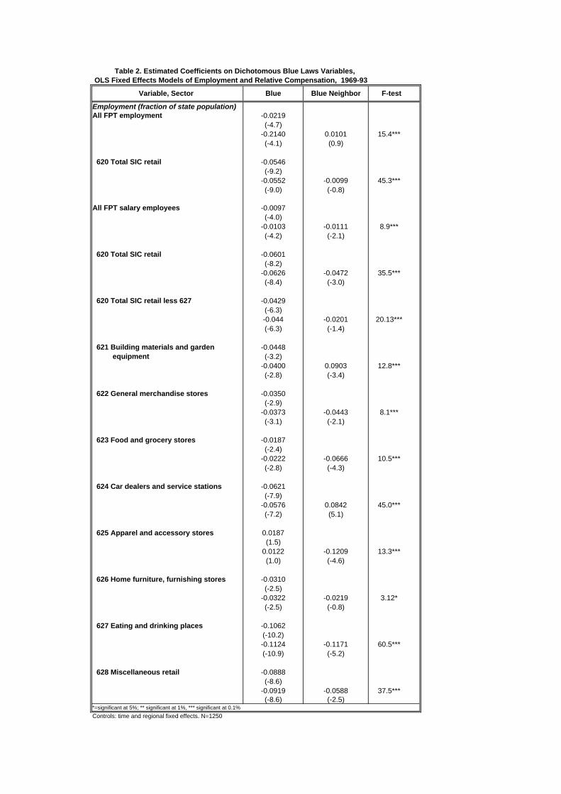
Table 2. Estimated Coefficients on Dichotomous Blue Laws Variables, OLS Fixed Effects Models of Employment and Relative Compensation, 1969-93

Employment (fraction of state population)All FPT employment -0.0219

(-4.7)-0.2140 0.0101 15.4***(-4.1) (0.9)

620 Total SIC retail -0.0546(-9.2)

-0.0552 -0.0099 45.3***(-9.0) (-0.8)

All FPT salary employees -0.0097(-4.0)

-0.0103 -0.0111 8.9***(-4.2) (-2.1)

620 Total SIC retail -0.0601(-8.2)

-0.0626 -0.0472 35.5***(-8.4) (-3.0)

620 Total SIC retail less 627 -0.0429(-6.3)-0.044 -0.0201 20.13***(-6.3) (-1.4)

621 Building materials and garden -0.0448 equipment (-3.2)

-0.0400 0.0903 12.8***(-2.8) (-3.4)

622 General merchandise stores -0.0350(-2.9)

-0.0373 -0.0443 8.1***(-3.1) (-2.1)

623 Food and grocery stores -0.0187(-2.4)

-0.0222 -0.0666 10.5***(-2.8) (-4.3)

624 Car dealers and service stations -0.0621(-7.9)

-0.0576 0.0842 45.0***(-7.2) (5.1)

625 Apparel and accessory stores 0.0187(1.5)

0.0122 -0.1209 13.3***(1.0) (-4.6)

626 Home furniture, furnishing stores -0.0310(-2.5)

-0.0322 -0.0219 3.12*(-2.5) (-0.8)

627 Eating and drinking places -0.1062(-10.2)-0.1124 -0.1171 60.5***(-10.9) (-5.2)

628 Miscellaneous retail -0.0888(-8.6)

-0.0919 -0.0588 37.5***(-8.6) (-2.5)

*=significant at 5%; ** significant at 1%, *** significant at 0.1% Controls: time and regional fixed effects. N=1250

Variable, Sector Blue Blue Neighbor F-test

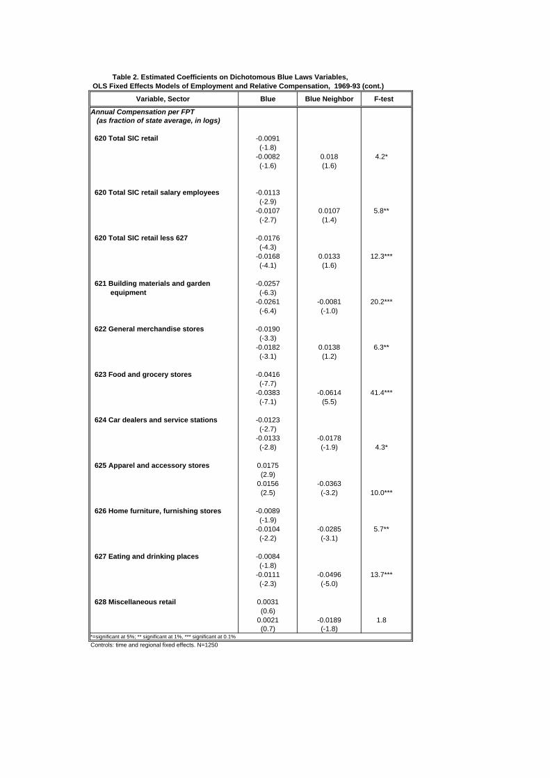
Table 2. Estimated Coefficients on Dichotomous Blue Laws Variables, OLS Fixed Effects Models of Employment and Relative Compensation, 1969-93 (cont.)

Annual Compensation per FPT (as fraction of state average, in logs)

620 Total SIC retail -0.0091(-1.8)

-0.0082 0.018 4.2*(-1.6) (1.6)

620 Total SIC retail salary employees -0.0113(-2.9)

-0.0107 0.0107 5.8**(-2.7) (1.4)

620 Total SIC retail less 627 -0.0176(-4.3)

-0.0168 0.0133 12.3***(-4.1) (1.6)

621 Building materials and garden -0.0257 equipment (-6.3)

-0.0261 -0.0081 20.2***(-6.4) (-1.0)

622 General merchandise stores -0.0190(-3.3)

-0.0182 0.0138 6.3**(-3.1) (1.2)

623 Food and grocery stores -0.0416(-7.7)

-0.0383 -0.0614 41.4***(-7.1) (5.5)

624 Car dealers and service stations -0.0123(-2.7)

-0.0133 -0.0178(-2.8) (-1.9) 4.3*

625 Apparel and accessory stores 0.0175(2.9)

0.0156 -0.0363(2.5) (-3.2) 10.0***

626 Home furniture, furnishing stores -0.0089(-1.9)

-0.0104 -0.0285 5.7**(-2.2) (-3.1)

627 Eating and drinking places -0.0084(-1.8)

-0.0111 -0.0496 13.7***(-2.3) (-5.0)

628 Miscellaneous retail 0.0031(0.6)

0.0021 -0.0189 1.8(0.7) (-1.8)

*=significant at 5%; ** significant at 1%, *** significant at 0.1% Controls: time and regional fixed effects. N=1250

Variable, Sector Blue Blue Neighbor F-test

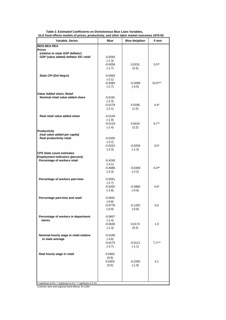
Table 2. Estimated Coefficients on Dichotomous Blue Laws Variables, OLS fixed effects models of prices, productivity, and other labor market outcomes 1976-93

REIS-BEA-REA Prices (relative to state GSP deflator) GSP (value added) deflator SIC retail -0.0043

(-1.3)-0.0059 0.0231 5.5**(-1.7) (3.3)

State CPI (Del Negro) -0.0063(-2.1)

-0.0083 -0.0289 10.6***(-2.7) (-4.5)

Value Added share, Retail Nominal retail value added share -0.0191

(-2.3)-0.0178 0.0185 4.4*(-2.1) (1.0)

Real retail value added share -0.0149(-1.9)

-0.0119 0.0416 6.7**(-1.4) (2.2)

Productivity (real value added per capita) Real productivity retail -0.0205

(-2.2)-0.0222 -0.0256 3.0*(-2.3) (-1.3)

CPS State count estimates Employment indicators (percent) Percentage of workers retail -0.4240

(-3.1)-0.4686 -0.6369 6.4**(-3.3) (-2.2)

Percentage of workers part-time -0.5051(-2.7)

-0.5252 -0.2880 4.6*(-2.8) (-0.9)

Percentage part-time and retail -0.0691(-0.8)

-0.0778 -0.1252 0.6(-0.9) (-0.8)

Percentage of workers in department -0.0657 stores (-1.4)

-0.0645 0.0174 1.0(-1.3) (0.2)

Nominal hourly wage in retail relative -0.0166 to state average (-3.6)

-0.0174 -0.0111 7.1***(-3.7) (-1.1)

Real hourly wage in retail 0.0463 (0.8)

0.0303 -0.2282 2.1(0.5) (-1.9)

*=significant at 5%; ** significant at 1%, *** significant at 0.1% Controls: time and regional fixed effects. N=1250

Variable, Sector Blue Blue Neighbor F-test

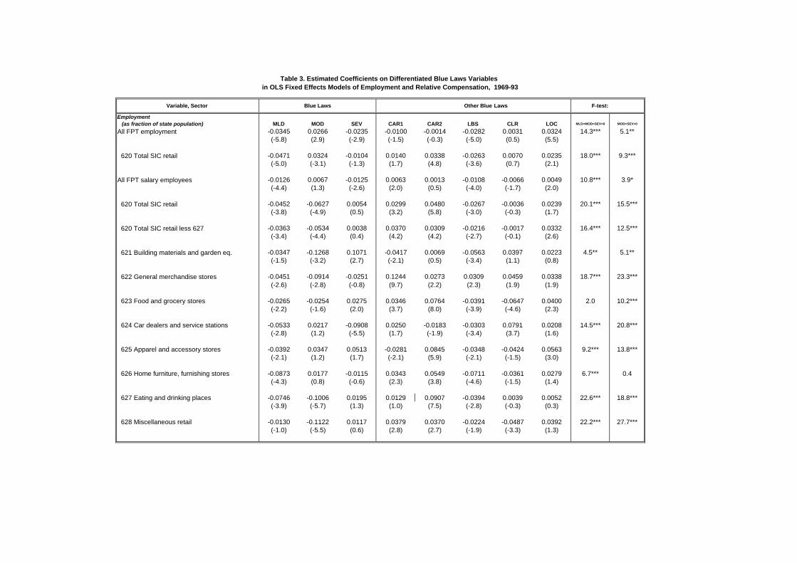
Table 3. Estimated Coefficients on Differentiated Blue Laws Variables in OLS Fixed Effects Models of Employment and Relative Compensation, 1969-93

Employment (as fraction of state population) MLD MOD SEV CAR1 CAR2 LBS CLR LOC MLD=MOD=SEV=0 MOD=SEV=0

All FPT employment -0.0345 0.0266 -0.0235 -0.0100 -0.0014 -0.0282 0.0031 0.0324 14.3*** 5.1**(-5.8) (2.9) (-2.9) (-1.5) (-0.3) (-5.0) (0.5) (5.5)

620 Total SIC retail -0.0471 0.0324 -0.0104 0.0140 0.0338 -0.0263 0.0070 0.0235 18.0*** 9.3***(-5.0) (-3.1) (-1.3) (1.7) (4.8) (-3.6) (0.7) (2.1)

All FPT salary employees -0.0126 0.0067 -0.0125 0.0063 0.0013 -0.0108 -0.0066 0.0049 10.8*** 3.9*(-4.4) (1.3) (-2.6) (2.0) (0.5) (-4.0) (-1.7) (2.0)

620 Total SIC retail -0.0452 -0.0627 0.0054 0.0299 0.0480 -0.0267 -0.0036 0.0239 20.1*** 15.5***(-3.8) (-4.9) (0.5) (3.2) (5.8) (-3.0) (-0.3) (1.7)

620 Total SIC retail less 627 -0.0363 -0.0534 0.0038 0.0370 0.0309 -0.0216 -0.0017 0.0332 16.4*** 12.5***(-3.4) (-4.4) (0.4) (4.2) (4.2) (-2.7) (-0.1) (2.6)

621 Building materials and garden eq. -0.0347 -0.1268 0.1071 -0.0417 0.0069 -0.0563 0.0397 0.0223 4.5** 5.1**(-1.5) (-3.2) (2.7) (-2.1) (0.5) (-3.4) (1.1) (0.8)

622 General merchandise stores -0.0451 -0.0914 -0.0251 0.1244 0.0273 0.0309 0.0459 0.0338 18.7*** 23.3***(-2.6) (-2.8) (-0.8) (9.7) (2.2) (2.3) (1.9) (1.9)

623 Food and grocery stores -0.0265 -0.0254 0.0275 0.0346 0.0764 -0.0391 -0.0647 0.0400 2.0 10.2***(-2.2) (-1.6) (2.0) (3.7) (8.0) (-3.9) (-4.6) (2.3)

624 Car dealers and service stations -0.0533 0.0217 -0.0908 0.0250 -0.0183 -0.0303 0.0791 0.0208 14.5*** 20.8***(-2.8) (1.2) (-5.5) (1.7) (-1.9) (-3.4) (3.7) (1.6)

625 Apparel and accessory stores -0.0392 0.0347 0.0513 -0.0281 0.0845 -0.0348 -0.0424 0.0563 9.2*** 13.8***(-2.1) (1.2) (1.7) (-2.1) (5.9) (-2.1) (-1.5) (3.0)

626 Home furniture, furnishing stores -0.0873 0.0177 -0.0115 0.0343 0.0549 -0.0711 -0.0361 0.0279 6.7*** 0.4(-4.3) (0.8) (-0.6) (2.3) (3.8) (-4.6) (-1.5) (1.4)

627 Eating and drinking places -0.0746 -0.1006 0.0195 0.0129 0.0907 -0.0394 0.0039 0.0052 22.6*** 18.8***(-3.9) (-5.7) (1.3) (1.0) (7.5) (-2.8) (-0.3) (0.3)

628 Miscellaneous retail -0.0130 -0.1122 0.0117 0.0379 0.0370 -0.0224 -0.0487 0.0392 22.2*** 27.7***(-1.0) (-5.5) (0.6) (2.8) (2.7) (-1.9) (-3.3) (1.3)

Variable, Sector Blue Laws Other Blue Laws F-test:

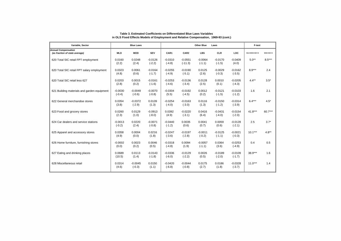
Table 3. Estimated Coefficients on Differentiated Blue Laws Variables in OLS Fixed Effects Models of Employment and Relative Compensation, 1969-93 (cont.)

Annual Compensation (as fraction of state average) MLD MOD SEV CAR1 CAR2 LBS CLR LOC MLD=MOD=SEV=0 MOD=SEV=0

620 Total SIC retail FPT employment 0.0160 0.0248 -0.0126 -0.0310 -0.0551 -0.0064 -0.0170 -0.0409 5.0** 8.5***(2.2) (2.4) (-2.2) (-4.8) (-11.3) (-1.1) (-1.5) (4.0)

620 Total SIC retail FPT salary employment 0.0323 0.0061 -0.0164 -0.0255 -0.0190 0.0125 -0.0029 -0.0162 8.9*** 2.4(4.8) (0.6) (-1.7) (-4.9) (-5.1) (2.6) (-0.3) (-3.5)

620 Total SIC retail less 627 0.0203 0.0015 -0.0161 -0.0253 -0.0136 0.0128 0.0010 -0.0205 4.4** 3.5*(2.8) (0.2) (-1.6) (-4.6) (-3.4) (2.5) (0.1) (-4.3)

621 Building materials and garden equipment -0.0030 -0.0049 -0.0070 -0.0304 -0.0192 0.0012 -0.0121 -0.0103 1.6 2.1(-0.4) (-0.6) (-0.8) (5.5) (-4.5) (0.2) (-1.5) (-1.2)

622 General merchandise stores 0.0354 -0.0372 0.0139 -0.0254 -0.0163 0.0116 -0.0150 -0.0314 6.4*** 4.5*(3.8) (-2.9) (1.3) (-4.0) (-3.0) (1.3) (-1.2) (-3.9)

623 Food and grocery stores 0.0260 0.0129 -0.0913 0.0392 -0.0220 0.0416 -0.0431 -0.0154 41.8*** 60.7***(2.3) (1.0) (-8.0) (4.9) (-3.1) (6.4) (-4.0) (-2.0)

624 Car dealers and service stations -0.0013 0.0220 -0.0071 -0.0440 0.0035 0.0041 0.0059 -0.0128 2.5 3.7*(-0.2) (2.4) (-0.8) (-1.2) (0.6) (0.7) (0.6) (-2.1)

625 Apparel and accessory stores 0.0358 0.0004 0.0216 -0.0247 -0.0197 -0.0011 -0.0125 -0.0021 10.1*** 4.8**(4.9) (0.0) (1.8) (-3.6) (-2.8) (-0.2) (-1.1) (-0.3)

626 Home furniture, furnishing stores -0.0002 0.0023 0.0046 -0.0318 0.0094 -0.0057 0.0364 -0.0253 0.4 0.5(0.0) (0.2) (0.5) (-4.8) (1.9) (-1.1) (3.6) (-4.9)

627 Eating and drinking places 0.0689 0.0113 -0.0143 -0.0336 -0.0129 0.0026 -0.0189 -0.0109 38.9*** 1.6(10.5) (1.4) (-1.8) (-6.0) (-2.2) (0.5) (-2.0) (-1.7)

628 Miscellaneous retail 0.0314 -0.0045 0.0150 -0.0420 -0.0044 0.0175 0.0186 -0.0328 11.0*** 1.4(4.6) (-0.3) (1.1) (-6.8) (-0.8) (2.7) (1.8) (-3.7)

F-test Other Blue Laws Variable, Sector Blue Laws

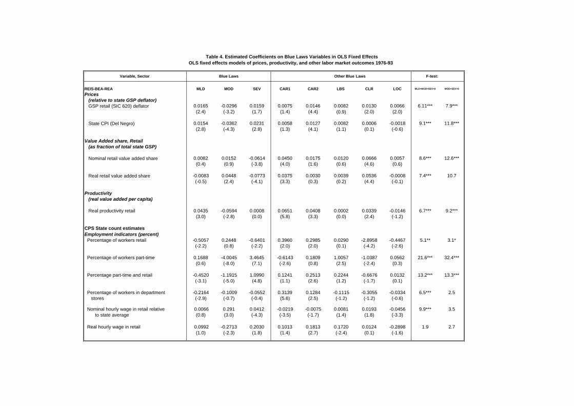
Table 4. Estimated Coefficients on Blue Laws Variables in OLS Fixed Effects OLS fixed effects models of prices, productivity, and other labor market outcomes 1976-93

REIS-BEA-REA MLD MOD SEV CAR1 CAR2 LBS CLR LOC MLD=MOD=SEV=0 MOD=SEV=0

Prices (relative to state GSP deflator) GSP retail (SIC 620) deflator 0.0165 -0.0296 0.0159 0.0075 0.0146 0.0082 0.0130 0.0066 6.11*** 7.9***

(2.4) (-3.2) (1.7) (1.4) (4.4) (0.9) (2.0) (2.0)

State CPI (Del Negro) 0.0154 -0.0362 0.0231 0.0058 0.0127 0.0082 0.0006 -0.0018 9.1*** 11.8***(2.8) (-4.3) (2.8) (1.3) (4.1) (1.1) (0.1) (-0.6)

Value Added share, Retail (as fraction of total state GSP)

Nominal retail value added share 0.0082 0.0152 -0.0614 0.0450 0.0175 0.0120 0.0666 0.0057 8.6*** 12.6***(0.4) (0.9) (-3.8) (4.0) (1.6) (0.6) (4.6) (0.6)

Real retail value added share -0.0083 0.0448 -0.0773 0.0375 0.0030 0.0039 0.0536 -0.0008 7.4*** 10.7(-0.5) (2.4) (-4.1) (3.3) (0.3) (0.2) (4.4) (-0.1)

Productivity (real value added per capita)

Real productivity retail 0.0435 -0.0594 0.0008 0.0651 0.0408 0.0002 0.0339 -0.0146 6.7*** 9.2***(3.0) (-2.8) (0.0) (5.8) (3.3) (0.0) (2.4) (-1.2)

CPS State count estimates Employment indicators (percent) Percentage of workers retail -0.5057 0.2448 -0.6401 0.3960 0.2985 0.0290 -2.8958 -0.4467 5.1** 3.1*

(-2.2) (0.8) (-2.2) (2.0) (2.0) (0.1) (-4.2) (-2.6)

Percentage of workers part-time 0.1688 -4.0045 3.4645 -0.6143 0.1809 1.0057 -1.0387 0.0562 21.6*** 32.4***(0.6) (-8.0) (7.1) (-2.6) (0.8) (2.5) (-2.4) (0.3)

Percentage part-time and retail -0.4520 -1.1915 1.0990 0.1241 0.2513 0.2244 -0.6676 0.0132 13.2*** 13.3***(-3.1) (-5.0) (4.8) (1.1) (2.6) (1.2) (-1.7) (0.1)

Percentage of workers in department -0.2164 -0.1009 -0.0552 0.3139 0.1284 -0.1115 -0.3055 -0.0334 6.5*** 2.5 stores (-2.9) (-0.7) (-0.4) (5.6) (2.5) (-1.2) (-1.2) (-0.6)

Nominal hourly wage in retail relative 0.0066 0.291 0.0412 -0.0219 -0.0075 0.0081 0.0193 -0.0456 9.9*** 3.5 to state average (0.8) (3.0) (-4.3) (-3.5) (-1.7) (1.4) (1.8) (-3.3)

Real hourly wage in retail 0.0992 -0.2713 0.2030 0.1013 0.1813 0.1720 0.0124 -0.2898 1.9 2.7(1.0) (-2.3) (1.8) (1.4) (2.7) (-2.4) (0.1) (-1.6)

F-test: Other Blue Laws Variable, Sector Blue Laws

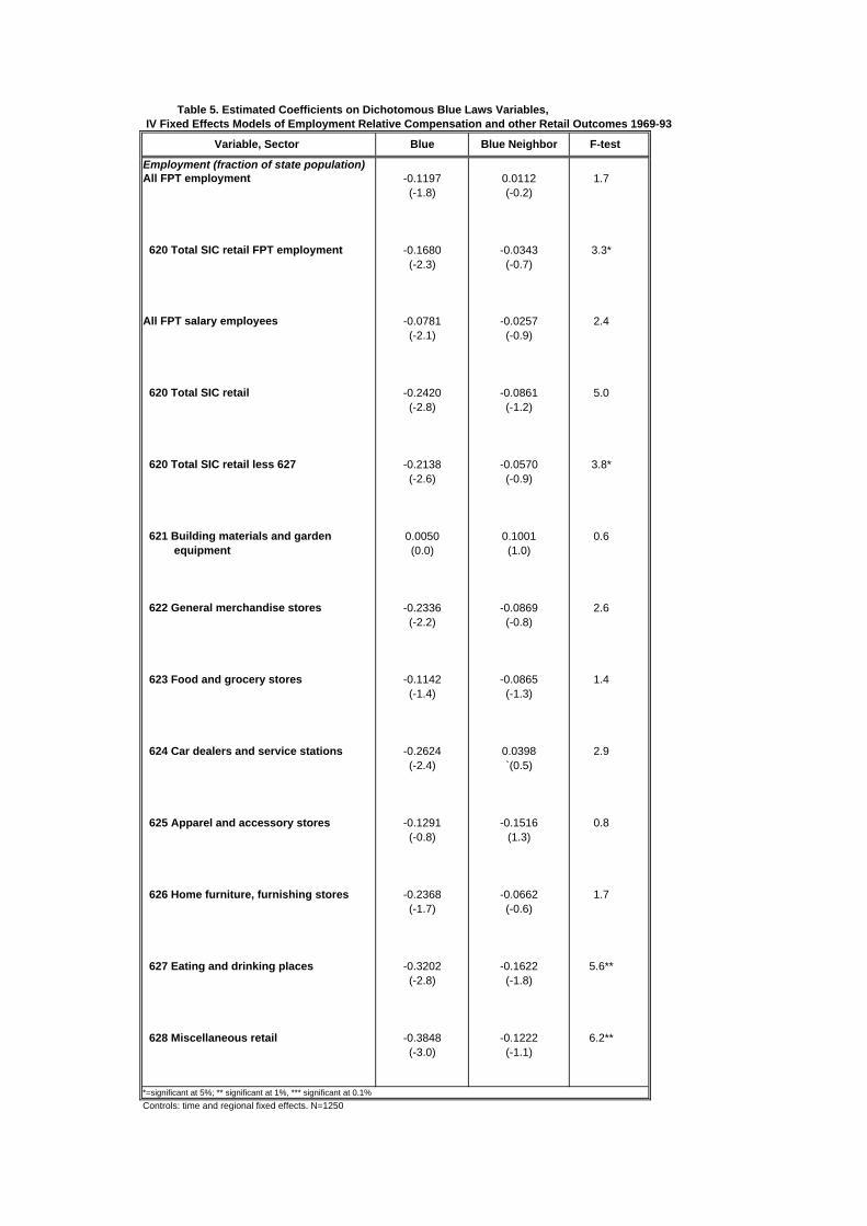
Table 5. Estimated Coefficients on Dichotomous Blue Laws Variables, IV Fixed Effects Models of Employment Relative Compensation and other Retail Outcomes 1969-93

Employment (fraction of state population)All FPT employment -0.1197 0.0112 1.7

(-1.8) (-0.2)

620 Total SIC retail FPT employment -0.1680 -0.0343 3.3*(-2.3) (-0.7)

All FPT salary employees -0.0781 -0.0257 2.4(-2.1) (-0.9)

620 Total SIC retail -0.2420 -0.0861 5.0(-2.8) (-1.2)

620 Total SIC retail less 627 -0.2138 -0.0570 3.8*(-2.6) (-0.9)

621 Building materials and garden 0.0050 0.1001 0.6 equipment (0.0) (1.0)

622 General merchandise stores -0.2336 -0.0869 2.6(-2.2) (-0.8)

623 Food and grocery stores -0.1142 -0.0865 1.4(-1.4) (-1.3)

624 Car dealers and service stations -0.2624 0.0398 2.9(-2.4) `(0.5)

625 Apparel and accessory stores -0.1291 -0.1516 0.8(-0.8) (1.3)

626 Home furniture, furnishing stores -0.2368 -0.0662 1.7(-1.7) (-0.6)

627 Eating and drinking places -0.3202 -0.1622 5.6**(-2.8) (-1.8)

628 Miscellaneous retail -0.3848 -0.1222 6.2**(-3.0) (-1.1)

*=significant at 5%; ** significant at 1%, *** significant at 0.1% Controls: time and regional fixed effects. N=1250

Variable, Sector Blue Blue Neighbor F-test

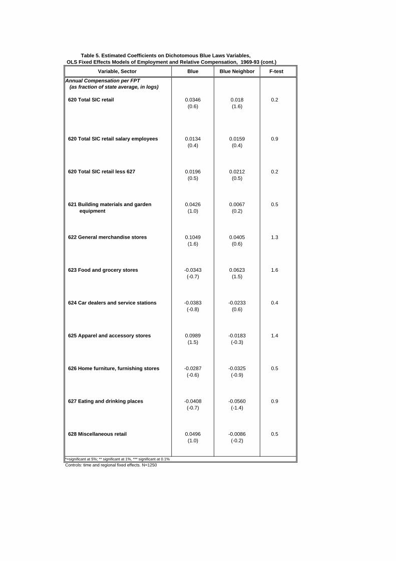
Table 5. Estimated Coefficients on Dichotomous Blue Laws Variables, OLS Fixed Effects Models of Employment and Relative Compensation, 1969-93 (cont.)

Annual Compensation per FPT (as fraction of state average, in logs)

620 Total SIC retail 0.0346 0.018 0.2(0.6) (1.6)

620 Total SIC retail salary employees 0.0134 0.0159 0.9(0.4) (0.4)

620 Total SIC retail less 627 0.0196 0.0212 0.2(0.5) (0.5)

621 Building materials and garden 0.0426 0.0067 0.5 equipment (1.0) (0.2)

622 General merchandise stores 0.1049 0.0405 1.3(1.6) (0.6)

623 Food and grocery stores -0.0343 0.0623 1.6(-0.7) (1.5)

624 Car dealers and service stations -0.0383 -0.0233 0.4(-0.8) (0.6)

625 Apparel and accessory stores 0.0989 -0.0183 1.4(1.5) (-0.3)

626 Home furniture, furnishing stores -0.0287 -0.0325 0.5(-0.6) (-0.9)

627 Eating and drinking places -0.0408 -0.0560 0.9(-0.7) (-1.4)

628 Miscellaneous retail 0.0496 -0.0086 0.5(1.0) (-0.2)

*=significant at 5%; ** significant at 1%, *** significant at 0.1% Controls: time and regional fixed effects. N=1250

Variable, Sector Blue Blue Neighbor F-test

Table 5. Estimated Coefficients on Dichotomous Blue Laws Variables, OLS fixed effects models of prices, productivity, and other labor market outcomes 1976-93

REIS-BEA-REA Prices (relative to state GSP deflator) GSP (value added) deflator SIC retail 0.0035 -0.0203 0.6

(0.1) (-0.8)

State CPI (Del Negro) -0.0181 -0.0318 1.0(-0.5) (-1.4)

Value Added share, Retail Nominal retail value added share 0.1449 0.0667 0.4

(0.9) (0.6)

Real retail value added share 0.1414 0.0870 0.6(1.0) (0.9)

Productivity (real value added per capita) Real productivity retail -0.2832 -0.1029 2.6

(-2.2) (-1.1)

Real productivity total state economy -0.4246 -0.1900 2.0(-1.9) (-1.2)

CPS State count estimates Employment indicators (percent) Percentage of workers retail -1.281 -0.8776 1.2

(-1.5) (-1.2)

Percentage of workers part-time 2.740 -0.679 0.8(1.2) (0.4)

Percentage part-time and retail -0.0498 -0.1169 0.0(-0.1) (-0.3)

Percentage of workers in department -0.2613 -0.0410 0.6 stores (-1.0) (-0.2)

Nominal hourly wage in retail relative -0.0108 -0.0138 0.2 to state average (-0.5) (-0.5)

Real hourly wage in retail -0.0584 -0.0512 1.2 (-1.2) (-1.1)

*=significant at 5%; ** significant at 1%, *** significant at 0.1% Controls: time and regional fixed effects. N=1250

Variable, Sector Blue Blue Neighbor F-test

Table 6. Blue Laws, Earnings and Employment in the March CPS, 1977-1993

MLD MOD SEV RTR*MLD RTR*MOD RTR*SEV MLD=MOD=SEV=0 MOD=SEV=0 RTR*MLD=RTR*MOD=RTR*SEV=0

RTR*MOD=RTR*SEV=0 N R²

Nominal weekly 0.005 0.011 -0.013 -0.016 0.076 -0.107 0.38 0.36 8.54*** 8.82*** 166236 0.464gross earnings (0.7) (0.6) (-0.7) (-1.1) (2.0) (-2,9)

Real weekly 0.012 -0.005 0.001 -0.019 0.078 -0.111 1.19 0.33 9.43*** 9.36 166236 0.421gross earnings (1.9) (-0.3) (0.1) (-1.3) (2.1) (-3,0)

Weekly hours 0.007 0.015 -0.015 -0.010 0.102 -0.119 1.15 0.63 9.32*** 11.67*** 159790 0.137(1.4) (1.1) (-1.1) (-0.9) (3.6) (-4.3)

Nominal hourly 0.005 -0.011 0.012 -0.036 -0.047 0.055 0.59 0.36 3.71* 1.88 159790 0.376wage (0.9) (-0,7) (0.8) (-2.8) (-1.5) (1.8)

Real hourly 0.006 -0.036 0.041 -0.040 0.016 -0.009 2.90* 3.57* 3.02* 0.47 159790 0.327wage (1.0) (-2.3) (2.6) (-3.0) (0.5) (-0.3)

*=significant at 5%; ***=significant at 1%; ***= significant at 0.1%

Dependent variable (in logs) OLS estimates of interaction of retail trade* with blue law: F-test:

FirstStageRegs.log----------------------------------------------------------------------------------------- log: C:\AtWork\Research\BlueLaws\2005AugBerlinFinale\FirstStageRegs.log log type: text opened on: 16 Sep 2005, 09:00:29

. reg blue region2-region8 y1970-y1993 larea lpop dems religion2 urban bluerel

Source | SS df MS Number of obs = 1250-------------+------------------------------ F( 37, 1212) = 30.23 Model | 144.998319 37 3.91887348 Prob > F = 0.0000 Residual | 157.104881 1212 .129624489 R-squared = 0.4800-------------+------------------------------ Adj R-squared = 0.4641 Total | 302.1032 1249 .241876061 Root MSE = .36003

------------------------------------------------------------------------------ blue | Coef. Std. Err. t P>|t| [95% Conf. Interval]-------------+---------------------------------------------------------------- region2 | .142984 .0496838 2.88 0.004 .0455083 .2404597 region3 | -.8660701 .0538176 -16.09 0.000 -.9716561 -.7604841 region4 | -.3482708 .0553645 -6.29 0.000 -.4568918 -.2396499 region5 | -.4125486 .0490918 -8.40 0.000 -.508863 -.3162342 region6 | -.268454 .0682078 -3.94 0.000 -.4022724 -.1346356 region7 | -.4770183 .06827 -6.99 0.000 -.6109587 -.3430779 region8 | -.4661851 .0703855 -6.62 0.000 -.604276 -.3280942 y1970 | -.047713 .0721033 -0.66 0.508 -.1891742 .0937483 y1971 | -.0500984 .0721028 -0.69 0.487 -.1915585 .0913617 y1972 | -.0696159 .0720867 -0.97 0.334 -.2110444 .0718126 y1973 | -.0709449 .0720873 -0.98 0.325 -.2123747 .070485 y1974 | -.1324361 .0727356 -1.82 0.069 -.2751377 .0102656 y1975 | -.1511024 .0727741 -2.08 0.038 -.2938797 -.0083252 y1976 | -.1989414 .0727336 -2.74 0.006 -.3416391 -.0562438 y1977 | -.2003362 .0727337 -2.75 0.006 -.343034 -.0576383 y1978 | -.1748881 .072267 -2.42 0.016 -.3166703 -.0331059 y1979 | -.1761744 .0722697 -2.44 0.015 -.3179619 -.0343869 y1980 | -.1632997 .0721488 -2.26 0.024 -.3048501 -.0217492 y1981 | -.163445 .072151 -2.27 0.024 -.3049997 -.0218902 y1982 | -.2263174 .0723477 -3.13 0.002 -.3682579 -.0843768 y1983 | -.2263662 .0723488 -3.13 0.002 -.3683091 -.0844234 y1984 | -.2024029 .0721877 -2.80 0.005 -.3440296 -.0607762 y1985 | -.2922748 .0724182 -4.04 0.000 -.4343537 -.1501959 y1986 | -.3316209 .0725644 -4.57 0.000 -.4739868 -.1892551 y1987 | -.3548831 .0726399 -4.89 0.000 -.4973971 -.2123691 y1988 | -.3557746 .072647 -4.90 0.000 -.4983024 -.2132468 y1989 | -.3553421 .0726461 -4.89 0.000 -.4978681 -.2128161 y1990 | -.3507816 .072623 -4.83 0.000 -.4932622 -.2083009 y1991 | -.3510695 .0726256 -4.83 0.000 -.4935553 -.2085837 y1992 | -.3752564 .072762 -5.16 0.000 -.5180099 -.2325029 y1993 | -.3757081 .0727658 -5.16 0.000 -.5184691 -.2329471 larea | -.0396257 .0172054 -2.30 0.021 -.0733814 -.00587 lpop | .1949255 .0174979 11.14 0.000 .1605961 .229255 dems | .4642864 .0808377 5.74 0.000 .305689 .6228837 religion2 | .0050572 .0011684 4.33 0.000 .0027649 .0073495 urban | -.0152149 .0012656 -12.02 0.000 -.0176979 -.0127318 bluerel | -.3172535 .0555771 -5.71 0.000 -.4262916 -.2082154 _cons | -.8864057 .2262548 -3.92 0.000 -1.3303 -.4425113------------------------------------------------------------------------------

. log close log: C:\AtWork\Research\BlueLaws\2005AugBerlinFinale\FirstStageRegs.log log type: text closed on: 16 Sep 2005, 09:00:39-----------------------------------------------------------------------------------------

Seite 1