Embed Size (px)
Citation preview

Discussion Papers
Diff erential Taxation and Firms' Financial LeverageEvidence from the Introduction of a Flat Tax on Interest Income
Frank Fossen und Martin Simmler
1190
Deutsches Institut für Wirtschaftsforschung 2012

Opinions expressed in this paper are those of the author(s) and do not necessarily reflect views of the institute. IMPRESSUM © DIW Berlin, 2012 DIW Berlin German Institute for Economic Research Mohrenstr. 58 10117 Berlin Tel. +49 (30) 897 89-0 Fax +49 (30) 897 89-200 http://www.diw.de ISSN print edition 1433-0210 ISSN electronic edition 1619-4535 Papers can be downloaded free of charge from the DIW Berlin website: http://www.diw.de/discussionpapers Discussion Papers of DIW Berlin are indexed in RePEc and SSRN: http://ideas.repec.org/s/diw/diwwpp.html http://www.ssrn.com/link/DIW-Berlin-German-Inst-Econ-Res.html
1
Differential taxation and firms’ financial leverage –
Evidence from the introduction of a flat tax on interest income1
Frank Fossen Martin Simmler2
Freie Universität Berlin, DIW Berlin
DIW Berlin and IZA
February 15, 2012
Abstract:
Tax competition for the mobile factor capital has led to a trend in many countries to levy
lower taxes on interest income, often introducing differential taxation between interest and
business income. In this study, we analyze the effect of such differential taxation on the debt
ratio of firms. We exploit a 2009 tax reform in Germany as a quasi‐experiment, which
introduced a flat final withholding tax and opened a gap of 18 percentage points between
the tax rate on income from unincorporated businesses and the new lower tax rate on
interest income. We apply a regression adjusted semi‐parametric difference‐in‐difference
matching strategy based on firm level panel data. In addition, we implement a more
structural approach with a tax rate differential, taking into account its endogeneity by using
instrumental variables. The results indicate that firms increase their leverage when the tax
rate on interest income decreases, albeit to a small degree.
Keywords: Income taxation, capital taxation, financial structure, leverage, matching
JEL Classification: H25, H24, G32
1 Acknowledgements: We would like to thank Jochen Bigus, Peter Haan, Jochen Hundsdoerfer, Viktor Steiner and participants at the Economic Policy Seminar and the FACTS Research Workshop at Freie Universität Berlin and at the Cluster Workshop at DIW Berlin for helpful and valuable comments. 2 Corresponding author, German Institute for Economic Research (DIW Berlin), 10108 Berlin, Germany, phone: +49 30 89789‐368, fax: +49 30 89789‐114, e‐mail: [email protected].

2
1 Introduction
Various countries have introduced flat rate taxes on capital income recently, typically with a
tax rate that is low in comparison to the progressive tax schedule applied to labor income and
other personal income sources. One reason for this trend may be international tax competition,
which incentivizes individual countries to tax the transnationally mobile factor capital more
lightly than more immobile factors such as labor (e.g. Devereux et al., 2008). We observe two
general approaches of how countries introduce low flat rate taxes on capital income. The first
approach is the Dual Income Tax (DIT) with its variants, as introduced primarily by Nordic
countries. The DIT is intended to treat all capital income the same, regardless of whether it
accrues from equity or credit capital. This gives rise to a practical problem, as it is difficult to
determine which part of the income of a firm’s owner-manager is capital income, which is
supposed to be taxed at the lower capital income tax rate, and which part is labor income, as
labor is supposed to be taxed at the higher labor income tax rate; usually, a normal return on
capital is assumed.
The second approach is the introduction of final withholding taxes on capital income, as
in Germany in 2009.3 Withholding taxes of the German type do not apply to business income
generated by unincorporated firms. This leads to a large gap (in Germany about 18.6
percentage points) between the tax rate on business income, which is taxed at the higher
personal income tax (PIT) rate for personal shareholders, and interest income, which is subject
to the lower final withholding tax.4 Thus, final withholding taxes avoid the practical problem
3 Similarly, Spain introduced a flat tax of 18% on interest income from instruments with a maturity of less than one year in 2007, and France implemented an optional flat tax on interest income with a rate of 18% in 2008. Other countries with this type of capital income taxes include Austria, the Czech Republic, Poland, and Portugal (OECD 2011, Table II.4). 4 Effectively, all equity income is taxed at a significantly higher rate than interest income. The tax on dividend income cumulates to a high rate that is similar to the tax rate on business income from unincorporated firms, because the corporate tax and the local business tax are not credited against the final withholding tax (see section 2).
of the DIT mentioned above, but at the cost of introducing differential taxation between
business income and interest income.
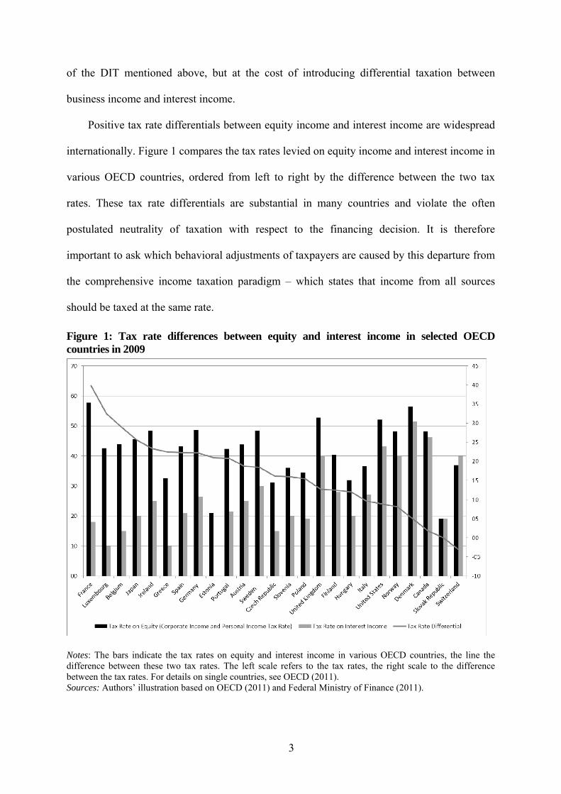
Positive tax rate differentials between equity income and interest income are widespread
internationally. Figure 1 compares the tax rates levied on equity income and interest income in
various OECD countries, ordered from left to right by the difference between the two tax
rates. These tax rate differentials are substantial in many countries and violate the often
postulated neutrality of taxation with respect to the financing decision. It is therefore
important to ask which behavioral adjustments of taxpayers are caused by this departure from
the comprehensive income taxation paradigm – which states that income from all sources
should be taxed at the same rate.
Figure 1: Tax rate differences between equity and interest income in selected OECD countries in 2009
Notes: The bars indicate the tax rates on equity and interest income in various OECD countries, the line the difference between these two tax rates. The left scale refers to the tax rates, the right scale to the difference between the tax rates. For details on single countries, see OECD (2011). Sources: Authors’ illustration based on OECD (2011) and Federal Ministry of Finance (2011).
3

4
When interest income is taxed at a lower rate than business income, we expect firms to
exploit this tax rate differential by increasing their debt ratios, i.e. total liabilities over total
assets. For example, an entrepreneur has incentives to reduce her equity stake in her business
in order to avoid the high tax on business income and invest her funds in the banking system
(or more generally the capital market) instead, where returns are taxed at the low tax rate on
interest income. Her business is then financed by the banking system in turn. We should thus
observe a higher debt ratio in the firm’s balance sheet.
This paper analyzes whether and how much firms adjust their financial structures in
reaction to differential taxation between business and interest income. Our hypothesis is that a
lower tax rate on interest income, relative to business income, increases the debt ratio.
To identify the effect, we exploit the introduction of the final withholding tax in
Germany in January 2009 as a quasi-experiment. As the tax gap between business and interest
income of 18.6 percentage points only opened up for personal shareholders, but not for
corporate shareholders, who are always taxed at the corporate tax rate regardless of their type
of income, the degree that this policy change affects a firm depends on the fraction of natural
persons in the ownership structure. This heterogeneity in exposure to the treatment between
firms allows us to identify the effect of the tax rate differential on the debt ratio chosen by
firms.
We apply a regression adjusted semi-parametric difference-in-difference matching
strategy based on firm level panel data to identify the effect of the differential taxation. This
approach accounts for a potential selection on observables as well as on time-invariant
unobservables and avoids functional form assumptions. In addition, we use a more structural
approach, where the debt ratio is modeled as a function of the effective tax rate differential,
which depends on the ownership structure, and other factors. This allows generalizing the
results and facilitates comparing them to extant literature. We use the instrumental variable
(IV) technique to account for potential endogeneity of the shareholder structure. As an
5
additional source of variation, we exploit local business tax rates, which differ across the more
than 10,000 German municipalities.
The results from the two approaches consistently indicate that a positive tax rate
differential between business income (high PIT rate) and interest income (low final
withholding tax rate) increases the debt ratio of firms, albeit only to a small degree. A cut in
the tax rate on interest income by 10 percentage points increases the debt ratio by 0.42
percentage points. Specifically, the introduction of the final withholding tax on capital income
in Germany in 2009 on average increased the debt ratio by about 1.4% relative to the average
debt ratio. We show that effects are stronger for smaller firms, firms that invest, firms not
carrying forward a loss from the previous year, and firms that do not appear to be constrained
on the credit market.
Our hypothesis, which states that a decrease in the personal tax rate on interest income
increases firms’ debt usage when the personal tax rate on business income remains constant,
is consistent with Miller (1977). He argues that the personal tax cost of interest income, which
was high relative to the personal tax cost of equity income in the USA at that time, could
explain why firms did not use more debt despite the tax benefits of interest deduction.5
Empirical evidence on the effect of differential taxation on the financial structure of
companies is scarce (see e.g. the survey of Graham, 2003). Using aggregate data, Gordon and
MacKie-Mason (1990) report that the debt ratios of corporations increased slightly in
response to the US Tax Reform Act of 1986, which increased the tax advantage of debt when
taking the personal tax into consideration. Graham (1999) and Alworth and Arachi (2001) rely
5 This tax benefits of debt result from the fact that interest expenses can be deducted from the tax base, whereas opportunity costs of equity cannot (see Graham, 2003, and Auerbach, 2002, for surveys, and Dwenger and Steiner, 2009, for a microdata study for Germany). The research question on how the corporate tax rate affects the use of debt financing as a tax shield differs from our research question on how a tax rate differential between equity returns and interest income affects the financing structure. As the corporate tax rate did not change between 2008 and 2009 in Germany, the general tax advantage of debt financing because of interest deduction remains constant in the period used in our main estimations and does not influence our analysis of changes in the debt ratio due to changes in the tax rate differential.

6
on heterogeneity between firms with respect to their payout policies to identify the effect of
personal taxation on the use of debt. They find a significant, positive effect of differential
taxation (defined as the difference between the tax rates on equity returns minus the tax rate
on interest income) on the ratio of debt/market value (Graham, 1999)6 and on the change of
the debt ratio (Alworth and Arachi, 2001). Studies that find that payout policies themselves
react to changes in taxation (Chetty and Saez, 2006; Jacob and Jacob, 2011) cast doubt on the
use of the payout ratio as identification strategy, however. Furthermore, firms that pay
dividends clearly differ from firms that do not, e.g. with respect to the (unobservable) degree
of financial constraints they face (Fazzari, Hubbard and Peterson, 1988, 2000). Using
international firm level data, Overesch and Voeller (2010) exploit variation in taxation
between European countries and find a significant negative effect of the tax rate on interest
income on the debt ratio of firms. Fuest and Weichenrieder (2002) use aggregated country
data and similarly find that lower taxes on personal interest income versus corporate income
decrease the share of corporate savings in total private savings. It remains an open question,
however, if the differences in firms’ debt policies found between the countries can be
interpreted as causal effects of taxation or at least partly stem from other differences between
the countries which cannot be completely controlled for.
This paper is structured as follows. In section 2 we describe how we exploit the 2009
German tax reform to identify the effect of differential taxation on the debt ratio. Section 3
details the empirical methodology, and section 4 introduces the individual firm panel data that
we use. In section 5 we present the results, while section 6 concludes the analysis.
6 In Graham (1999), the estimated coefficient is negative, because the tax rate differential is defined as the tax rate on interest income minus the tax rate on equity returns.
7
2 German tax reform as a quasi-experiment
To identify the effect of a tax rate differential between business income and interest income
on the debt ratio, we exploit the introduction of the flat final withholding tax in Germany in
January 2009 as a quasi-experiment. This reform substantially reduced the tax rate on interest
income for personal taxpayers in the highest PIT bracket from 44.3% PIT7 in 2008 to 26.4%
final withholding tax8 in 2009. In contrast, the top marginal tax rate on income from
unincorporated businesses remained unchanged at about 45% at the level of the personal
shareholder.9 Thus, the tax reform in 2009 led to a large gap of 18.6 percentage points
between the unchanged top marginal tax rate on business income and the new low flat tax rate
on interest income.
Similarly to the top marginal tax rate on business income, the top marginal cumulative
tax rate on dividends also remained nearly unchanged at about 49% at the shareholder level in
2009.10 Thus, taxation of equity returns did not change significantly in 2009, regardless of
whether they accrued from unincorporated businesses (business income) or corporations
(dividend income). So in principle the differential taxation effect we are investigating affects
both unincorporated businesses and corporations similarly. In the empirical analysis, we focus
on unincorporated partnership businesses for reasons we explain in section 4.
7 The rate of 44.3% refers to the marginal PIT rate of 42%, which was applicable for taxable income in the bracket between €52,152 (about US$ 73,000 on 1/1/2009) and €250,000 (US$351,000) in 2007-2008 and between €52,552 and €250,400 in 2009 for single tax filers (or double these amounts for married joint filers), plus the mandatory so-called solidarity surcharge. In 2007, a new top PIT bracket, the so called “rich tax”, above this bracket was introduced with a marginal PIT rate of 45% (47.5% including the solidarity surcharge). It became effective for business income one year later in January 2008. In the following, we assume that most shareholders of partnership businesses fall into the former top income tax bracket, but not into the new “rich tax” bracket, so we will use the marginal tax rate of 44.3% in our calculations. 8 The rate of 26.4% refers to 25% final withholding tax plus solidarity surcharge. 9 This rate refers to the PIT and solidarity surcharge rate of 44.6%, as explained above, plus the local business tax, which is largely credited against the PIT. If the local business tax rate, which is set by the municipality, is high, the local business tax cannot be credited completely, which explains the average rate of about 45%. 10 Before 2009, the tax rate on dividends was calculated as corporate tax + solidarity surcharge + local business tax + 50% dividend taxation rule for the PIT (shareholder-relief system); the last summand was replaced by the final withholding tax on the full dividend in 2009, which yields a similar tax rate for shareholders in the top PIT bracket.
8
Importantly, the large tax gap between business and interest income only opens up for
firms with natural persons as shareholders, who are subject to the PIT. Firms with exclusively
corporations as shareholders are unaffected by the introduction of the final withholding tax,
because corporate shareholders are always taxed at the tax rate for corporations of about
29.9%, regardless of whether they derive interest income or income from equity holdings.11
Therefore, the degree the introduction of the final withholding tax affects a firm depends on
the fraction of natural persons in the ownership structure. The larger the fraction of personal
shareholders as opposed to corporations, the higher the potential benefit from the reform. This
heterogeneity in exposure to the treatment allows us to identify the effect of the tax rate
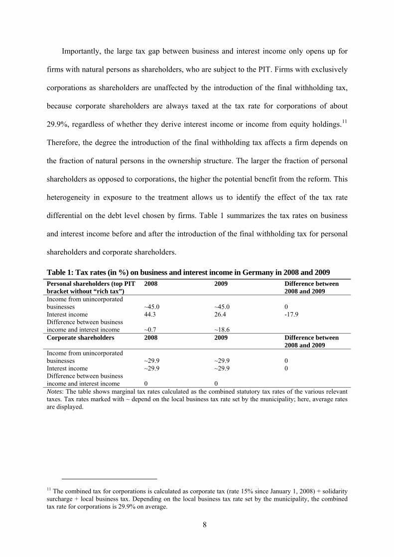
differential on the debt level chosen by firms. Table 1 summarizes the tax rates on business
and interest income before and after the introduction of the final withholding tax for personal
shareholders and corporate shareholders.
Table 1: Tax rates (in %) on business and interest income in Germany in 2008 and 2009 Personal shareholders (top PIT bracket without “rich tax”)
2008 2009 Difference between 2008 and 2009
Income from unincorporated businesses ~45.0 ~45.0 0 Interest income 44.3 26.4 -17.9 Difference between business income and interest income ~0.7 ~18.6 Corporate shareholders 2008 2009 Difference between
2008 and 2009 Income from unincorporated businesses ~29.9 ~29.9 0 Interest income ~29.9 ~29.9 0 Difference between business income and interest income 0 0 Notes: The table shows marginal tax rates calculated as the combined statutory tax rates of the various relevant taxes. Tax rates marked with ~ depend on the local business tax rate set by the municipality; here, average rates are displayed.
11 The combined tax for corporations is calculated as corporate tax (rate 15% since January 1, 2008) + solidarity surcharge + local business tax. Depending on the local business tax rate set by the municipality, the combined tax rate for corporations is 29.9% on average.
9
Another independent source of variation is the local business tax.12 Its rates vary not just
across the more than 10,000 municipalities in Germany, but also over time, because
municipalities are entitled to determine their own multipliers (local business tax rate = 0.035 *
multiplier/100) and change them at anytime.13 For personal shareholders of unincorporated
businesses, the local business tax is largely credited against the PIT. The marginal local
business tax burden that remains after crediting is calculated as
= [multiplier/100 – min(3.8; multiplier/100)*1.055]*0.035. (1)
Thus, if the multiplier equals 380*1.055=400.9, it is fully credited against the PIT (if the PIT
liability is sufficiently high); if it is higher, a positive tax burden remains; and if it is lower,
there is partial overcompensation (due to the solidarity surcharge that introduces the factor
1.055). Simulations using the microsimulation model BizTax for business taxation (Bach and
Fossen, 2008) indicate that in 2008, about a quarter of all unincorporated businesses in
Germany could not fully credit their local business tax against the PIT because the local
business tax multiplier was too high. In our sample, the distribution of the local business tax
burden for income from unincorporated businesses with exclusively natural persons as
shareholders has a mean of 0.12% and a standard deviation of 1.02; the minimum is -0.73%
and the maximum 3.11%. For the identification of the effect of the tax rate differential
between business income and interest income on the debt ratio, the important point is that the
higher the local business tax rate, the higher the combined tax rate on business income for
personal shareholders (which is 45% on average), and thus the larger the tax rate differential
introduced by the 2009 reform.
12 The German local business tax is a subject of research in the context of tax competition and fiscal equalization transfers (Buettner, 2006; Egger et al., 2010). 13 The uniform basic tax rate was reduced from 0.05 to 0.035 on January 1, 2008, along with other changes that partly offset this tax rate reduction. The local business tax is mostly a tax on profits, although some additions and reductions apply, e.g. financing expenses are partly added back to the local business tax base (Bach and Fossen, 2008). For companies operating in multiple municipalities, the total tax base is distributed according to an apportionment formula, and each municipality applies its multiplier to its allocated share. As we can only observe a company’s registered office, we can only use the multiplier associated with this location.

10
3 Methodology
3.1 Regression-adjusted semi-parametric difference-in-difference matching strategy
To analyze how the differential taxation of business and interest income affects the debt ratio
of firms, we use two different methodologies. The first approach is derived from the
evaluation literature; specifically, we implement a regression-adjusted semi-parametric
difference-in-difference matching strategy similar to Heckman et al. (1997). The second is a
more structural approach that is more comparable to the extant empirical literature on taxes
and corporate finance: We regress the debt ratio on the tax rate differential and control
variables (in first differences and accounting for the endogeneity of the tax rate differential).
In this section, we first describe the matching approach, and proceed with the more structural
approach in section 3.2.
The difference-in-difference matching technique has two main advantages. Firstly, it
accounts for potential selection on observables and on time-invariant unobservables, and,
secondly, it avoids reliance on functional form assumptions.
As explained above, we base our identification strategy on the share of natural persons in
a firm’s shareholder structure.14 We define treatment and control groups for matching as
follows. As the introduction of the final withholding tax in Germany in 2009 reduced the tax
rate on interest income for natural persons as shareholders, but not for corporations as
shareholders, firms belong to the treatment group when more than half of their equity is held
by natural persons in Germany. The control group consists of firms with more than half of
their equity held by corporations. We consider the cut-off point of 50% reasonable because
the majority of the shareholders in terms of equity held are likely to dominate the financing
14 The variation in local business tax rates is used in the second, more structural approach only.
11
decisions of the firm. However, the results are not very sensitive to different choices of this
threshold.
Matching methods solve the fundamental problem of the unobserved counter-factual: If
the same company could be observed both with and without the treatment (i.e. the reduction
of the tax rate on interest income on January 1, 2009), the causal effect of the treatment on the
outcome (i.e. the change in the debt ratio between 2008 and 2009) would simply be the
difference in the outcome. The idea of the matching method is to compare treated and control
companies that are sufficiently similar to derive the causal effect. One matches treatment and
control group observations on a set of all relevant variables X such that the conditional mean
independence assumption is fulfilled.15 If we used standard matching, in this application the
assumption would be that the expectation of the debt ratio would be identical for the treatment
and control groups in the absence of the tax reform, conditional on the matching variables.
As we have access to panel data, we are able to apply difference-in-difference matching
instead, which relies on the considerably less restrictive assumption that the expected change
in the debt ratio between 2008 and 2009 would be the same for the treatment and control
observations in the absence of the policy change. This accounts for potential unobserved time-
invariant differences between treatment and control groups, which might be correlated both
with treatment assignment and the debt ratio. Unexplained differences in the level of the debt
ratio between firms with different shareholder structures thus do not bias the results from
difference-in-difference matching.
A crucial requirement is that all relevant variables that affect treatment assignment and
the outcome are included in X for matching (ignorable treatment assignment assumption).
Based on the literature of organizational choice, we include the debt ratio (total liabilities/total
book assets), log firm size (balance sheet total in thousand euro), tangibility (ratio tangible
15 Stuart (2010), Caliendo and Kopeinig (2008) and Caliendo and Künn (2011) provide comprehensive overviews and an application of matching methods.
assets/total assets), log firm age (in years), the local business tax rate, as well as fifteen
industry dummy variables, to capture differences in diversifiable risk. For matching we use
the 2008 values of these variables, i.e. the values before the tax reform. In additional
specifications, we further add the ratio of EBITDA (earnings before interest, taxes,
depreciation and amortization) over total assets in X. In these estimations, a large number of
firms have to be excluded from the sample, however, because these firms only provide
balance sheet information and the required income statements are not available.
Since X includes various continuous variables, we use the estimated one-dimensional
propensity score to define proximity between observations. The propensity score is the
probability of receiving treatment, i.e. the probability of being a firm with more than half of
its equity held by personal shareholders, conditional on X. Rosenbaum and Rubin (1985)
show that conditioning on X is equivalent to conditioning on the propensity score. The
propensity score is estimated by running a logistic regression of the treatment indicator on X.
As distance measure we use the linear propensity score,16 which improves the balance
between the treatment and control groups (Rosenbaum and Rubin, 1985).
For matching treatment and control group observations, we use the semi-parametric
approach of kernel matching. For each treated firm, we assign a kernel-weighted outcome
average of the control group observations. The shorter the distance between a treated and a
non-treated observation, the greater is the weight. Due to its superiority in terms of efficiency,
we choose the Epanechnikov kernel (Cameron and Trivedi, 2006).17 To test the sensitivity of
our matching strategy, we also apply a 5-to-1 nearest neighbor caliper matching.18 This
strategy assigns the five closest control group observations to a treatment group observation.
12
16 This distance measure is given by , where ek is the propensity score for observation k. 17 As bandwidth parameter, we follow Heckman et al. (1997) and choose 0.06. 18 Matching strategies differ by their weighting functions. Heckman et al. (1997) and Smith and Todd (2005) advocate kernel matching.

13
The caliper prevents poor matches by ensuring that no observations are matched that are too
distant in terms of the linear propensity score. We apply a caliper of 0.25 standard deviations
of the estimated linear propensity score as proposed by Rosenbaum and Rubin (1985).19
We match control observations to the treated firms with replacement. This can improve
balance since control firms that are similar to multiple treated observations may be used
multiple times (Stuart, 2010). Furthermore, we restrict the analysis to the region of common
support, i.e. we drop treatment observations with a linear propensity score exceeding the
maximum or falling below the minimum linear propensity score of the control group.
The last feature of our matching strategy is the regression adjustment. Since matching
estimators can be rewritten as weighted regressions, it is also possible to include additional
control variables in the regression that potentially affect the outcome. Although this is not
necessary for consistency if the propensity score is modeled correctly, it improves the
efficiency of the regression. Moreover, Bang and Robbins (2005) show that regression-
adjusted matching estimators remain consistent if either the propensity score model or the
regression model is specified correctly. Thus, regression-adjusted matching can be considered
double-robust.
The dependent variable in the regression adjustment is the outcome variable, i.e. the
change in the debt ratio between 2008 and 2009. The regressor of main interest is the binary
treatment indicator that equals one for firms with more than half of their equity held by
persons, and zero otherwise. Additional covariates, all in first differences, are log firm size,
tangibility, log firm age, and EBITDA/total assets (the latter in some specifications only
because of missing values). Since tangibility and firm size might be affected by changes in the
19 Rosenbaum and Robin (1985) show that a caliper of 0.2 standard deviations removes 98% of the bias in a normally distributed covariate and propose 0.25 standard deviations of the linear propensity score as caliper.

financial structure, we include lagged values of these control variables, i.e. their changes
between 2007 and 2008.20
We use Huber-White heteroscedasticity robust standard errors in our analysis, not least
because estimated propensity scores are used for the weighting of the regression. There is
some evidence that using an estimated propensity score leads to an overestimation of the
variance of the estimated coefficients (Stuart, 2010) and thus yields conservative confidence
levels. We confirm this conjecture for our application, as we obtain generally smaller standard
errors in a robustness check when we use bootstrapping to estimate standard errors.
3.2 Structural approach
Our second, more structural approach has the advantage of being more directly comparable to
the extant empirical literature on taxation and finance because we estimate a coefficient of a
tax rate differential that may be compared across time and location contexts. Considering a
continuous tax rate differential instead of a binary treatment indicator also implies that we use
more information. Furthermore, in this approach we exploit additional variation through the
local business tax rate, which varies across the more than 10,000 municipalities in Germany.
The disadvantage in comparison to the semi-parametric matching approach is the necessity of
a functional form assumption.
We estimate linear approximations of the relationship between the debt ratio and the tax
rate differential of the form
ittiitdiffit
it
Xassetstotal
debttotal
, (2)
20 The results do not change when we use an IV approach instead, where we include the potentially endogenous change of these two control variables between 2008 and 2009 and use the twice-lagged levels as their IVs. In the specifications including the change in the ratio EBITDA/total assets, we also use its twice lagged level as its IV, as it might be endogenous as well.
14

where the dependent variable is the debt ratio of company i in year t, itdiff is the tax rate
differential between the tax rates on business income and interest income effective for i in t
(with coefficient ), Xit is a vector of control variables (with coefficient vector ), i and t
are unobserved firm- and time-specific effects, it is an idiosyncratic error term, and is a
constant. i could capture unobserved firm-specific costs of debt usage, for example, and t
reflects the influence of the business cycle, which is especially relevant in the period under
consideration because of the world-wide financial and economic crisis (although the effects
were not as severe in Germany as in other countries).
The firm-specific tax rate differential is calculated as a weighted difference between the
tax rates on business and interest income:
)(1
interestjt
businessjit
J
jjit
diffit
it
, (3)
where Jit is the number of shareholders and jit is the equity share of shareholder j in firm i in
year t. The statutory tax rates on business income jitbusiness and interest incomejt
interest depend
both on the type of shareholder j and the year t; most importantly, jtinterest was decreased in
2009 for personal, but not corporate shareholders, as explained in section 2.21 Furthermore,
jitbusiness depends on the local business tax rate levied in the municipality where firm i is
located (section 2).
As control variables, in Xit, we include non-tax determinants of the debt ratio, i.e. lagged
log firm size, lagged tangibility and log firm age. In some specifications, we additionally
include the ratio EBITDA/total assets, excluding firms with missing income statements from
the sample. To eliminate the unobserved firm-specific effects i, we estimate equation (2) in
21 Since we do not observe total income of shareholders, we follow Rajan and Zingales (1995) as well as Overesch and Voeller (2010) and assume for the calculation of the tax rate differential that personal shareholders are in the highest PIT bracket (without the “rich tax”, see section 2).
15

first differences. In additional estimations based on more than the two years 2008 and 2009,
we also include time dummy variables to control for the business cycle effects t.
A firm’s ownership structure, which is captured by the weights jit, may itself be affected
by taxes, which could lead to endogeneity of the tax rate differential (3). We account for this
potential endogeneity with an IV approach. The idea is similar to Gruber and Saez (2002). To
construct the instrument, we simulate the tax rate differentials in 2008 and 2009 that would
have prevailed had the shareholder structure remained unchanged since 2007; in other words,
we use ji,2007 in the calculation of i,2008diff,iv and i,2009
diff,iv to avoid introducing the potentially
endogenous weights ji,2009 that may have been affected by the tax reform (to be sure, we also
avoid ji,2008 which might partly anticipate the tax reform). We then use the difference
i,2009diff,iv - i,2008
diff,iv as the IV for the first differenced tax rate differentiali,2009diff - i,2008
diff.
There is no endogeneity of tax rates with respect to other firm characteristics such as a firm’s
profits because we use combined statutory tax rates, which provide sufficient variation.
As mentioned before, in our main estimations we use the years immediately prior to and
after the reform only, i.e. 2008 and 2009. In further estimations, we also use years back to
2004.22 In these latter estimations, we additionally control for the combined tax rate on
business income effective for firm i in year t. As our estimation sample is comprised of
partnership businesses that divide their income among and pass it through to the shareholders
(see section 4), the effective tax rate on business income again depends on the shareholder
structure:
businessjit
J
jjit
businessit
it
1
~ . (4)
16
22 The instrument for the change in the tax rate differential is calculated the same way in all the years, analogous to what we describe above for the change between 2008 (period t-1) and 2009 (period t), i.e. we use the twice lagged shareholder structure (ji,t-2) to simulate the tax rate differentials i,t-1
diff,iv and itdiff,iv.

The identifiers in this weighted sum are defined as above. This control variable is important
when including years both before and after 2008, because the statutory corporate income tax
rate (CIT) was decreased from 25% to 15% on January 1, 2008, which decreased jitbusiness
when shareholder j is a corporation. This control variable thus accounts for the effect of the
business income tax rate on the use of debt financing as a tax shield because of the
deductibility of interest payments from the tax base (see footnote 5). To avoid potential
endogeneity due to changing shareholder structures, we instrument businessit~ with a simulated
business tax rate ivbusinessit
,~ using the twice-lagged shareholder structure, completely analogous
to our instrument for the tax rate differential. When we base our estimations on 2008 and
2009 only, it is not necessary to separately control for the tax rate on business income, as it
did not change between these years and is thus included in the firm specific fixed effects i,
which are eliminated by first differencing the data.23
4 Individual firm panel data
The database for our study is the comprehensive financial statements collection Dafne
provided by Bureau van Dijk. The panel data contain individual balance sheets, income
statements and detailed ownership information for German firms. The main source for this
database is the official registrar of companies in Germany. Since 2006 the database has
covered nearly all publishing companies in Germany; these are firms with limited liability, as
they have to obey legal publication requirements.24 Before, primarily larger companies were
included in Dafne. In our baseline estimations, we use the years immediately prior to and after
23 Strictly speaking, this is only true when the shareholder structure remains constant between these two years. In our sample only about 2% of the firms exhibit any changes in their shareholder structure between 2007 and 2009. If we include the business income tax rate as a control variable in the estimations based on 2008 and 2009 only, it is insignificant and can thus be dropped from the final specification. 24 Corporations have to publish their financial statements according to §325 German Commercial Code. The same publication requirements apply also to unincorporated firms with limited liability (such as the legal form GmbH & Co. KG, which is explained further below).
17
18
the introduction of the final withholding tax, i.e. 2008 and 2009. In additional estimations, we
include all years back to 2004; there is no sufficient data for more recent years. We merge
local business tax rates provided by the Statistical Offices (2004-2009) to the database by
using the firms’ postal codes as provided in Dafne.
In this study we focus on partnership businesses, which represent a widespread and
important legal form in Germany. In 2009, partnerships accounted for 38% of aggregate
taxable turnover in Germany (Federal Statistical Office, 2011). They are comparable to S-
corporations in the United States. The main reason for our choice is that in addition to the tax
reform of interest on January 1, 2009, there was a business tax reform that came into effect
January 1, 2008, which primarily affected corporations; the most important change was a
reduction in the CIT rate from 25% to 15%. Therefore, for corporations it is more difficult to
disentangle potential delayed effects of the 2008 reform from the effects of the introduction of
the final withholding tax a year later.25 As in other countries, partnerships in Germany are not
legal entities and therefore not subject to the CIT. Instead, profits of partnerships are subject
to the PIT of the receiving shareholders according to the tax transparency principle (as
opposed to the deferral principle for corporations). In addition, partnerships are subject to the
local business tax at the firm level; the local business tax is largely credited against the PIT of
personal shareholders, however, as explained in section 2.
Changes in the taxation of incorporated and unincorporated businesses could influence
organizational choice, as suggested by the literature, which is mostly based on US data
(Gordon and MacKie-Mason 1994; Goolsbee, 1998, 2004).26 However, we observe only 32
25 The introduction of the final withholding tax in 2009 was also somewhat more complicated for corporations than for partnerships. First, the shareholder relief system for dividends was replaced with the final withholding tax (although this did not change the effective tax burden for shareholders in the highest PIT bracket, see footnote 10). Second, capital gains, which before 2009 were tax exempt when the equity was held for more than a year, became subject to the new final withholding tax if the equity was acquired on or after January 1, 2009. 26 Using time series data for 1900 to 1939, Goolsbee (1998) finds only small effects of taxes on the organizational form, whereas in Goolsbee (2004) he reports much larger effects based on cross-sectional data. Thoresen and Alstadsaetter (2008) find that the introduction of a Dual Income Tax increases the probability of

19
changes of the legal form from unincorporated to incorporated businesses and 81 changes
from incorporated to unincorporated business between 2007 and 2009 in our sample of 38,339
firms, so this adjustment channel does not seem to be relevant for our study. High costs
involved in changing legal forms in Germany may explain why we do not observe more
changes. Moreover, reorganization is often accompanied by the disclosure of hidden assets,
which firms may want to avoid.
We base our analyses on limited partnership firms with a limited liability company as
general partner (GmbH & Co. KG). About a third of all partnership firms in Germany
(without sole proprietorships) had this legal form in 2009 (Federal Statistical Office, 2011).
These firms have limited liability similar to corporations due to the limited liability company
as general partner. These partnerships are well represented in our database, because due to the
limited liability strict publication requirements apply for them that are very similar to those of
corporations.
From the estimation sample we exclude firms without corporate or personal shareholders
because of the different taxation rules for banks and trusts; where less than 75% of the
shareholders are domestic; or where less than 75% of the shareholder structure is observed.27
Further, we drop firms with liabilities above €20 million (about US$ 28 million on 1/1/2009),
as these firms are potentially affected by the interest ceiling rule, which was introduced in
January 2008 and limited the deductibility of net interest payments above one million euro
from the tax base (assuming an interest rate of 5%).28 Financial and holding companies are
excluded from the sample as well because of their different determinants of the debt ratio. The
incorporation for an active owner of a human capital intensive business. The reason is that in case of incorporation all income is subject to the relatively low tax rate on capital income, whereas otherwise income is split up into labor and capital income assuming a normal return on capital, which results in a higher overall tax burden. 27 In two robustness checks, we required that 60% (90%, resp.) of the shareholders structure be observed. The results did not change significantly. 28 In fact for 2008 the threshold of the interest ceiling rule amounts to three million euro, since the German government increased the threshold retroactively in spring 2009. Due to the retroactive change we only include firms with interest expenses below the lower threshold.
20
final estimation sample used in our main specifications comprises 76,678 firm-years in 2008
and 2009 and 125,368 firm-years over the larger time frame between 2004 and 2009.
The outcome variable, the debt ratio of the firms, is calculated as the ratio of total
liabilities/total book assets. In our estimations of the effect of differential taxation on the debt
ratio, we follow the extant literature and consider the following non-tax factors as control
variables (all monetary variables are deflated using the Consumer Price Index):
Firm size: The firm size may indirectly influence the financial structure as it might be a
proxy for the quality of information available to outside investors, because publication
requirements are linked to size criteria (Chan, Faff and Ramsay, 2005). Lower uncertainty due
to better information could increase the equity share since issuing equity is sensitive to
information. Thus, we control for firm size and measure it as the natural logarithm of the real
book value of total assets.
Age of the firm: According to the life cycle hypothesis (e.g. DeAngelo et al., 2006), older
firms are likely to have greater free cash flow. They may thus accumulate larger amounts of
retained earnings, which would decrease the debt ratio. We use the natural logarithm of the
firm age in years.
Tangibility: The extant literature suggests two opposing possible effects of tangibility on
the use of debt. Harris and Raviv (1990) as well as Almeida and Cambello (2007) find a
positive correlation between a company’s liquidation value (which is increasing in the
tangibility of a firm's assets) and the optimal debt level since a higher liquidation value
reduces costs for debt holders in comparison to equity holders. On the other side, DeAngelo
and Masulis (1980) argue that firms with a high share of tangible assets have higher
depreciation allowances and thus benefit from this non-debt tax shield, which reduces
incentives to use debt as a tax shield. We measure tangibility as the ratio tangible assets/total
book assets.
21
Profitability: As common in the literature (i.e. Rajan and Zingales, 1995, and Graham,
1999), we control for company’s profitability in some specifications. Our measure of
profitability is the ratio EBITDA/total book assets. As income statements are necessary to
calculate this variable, which are missing for most firms, we only include this variable in
additional specifications.
Loss in the previous year: A company that is carrying forward a loss can offset current
profits against these former losses and thus has lower incentives to make use of the
preferential taxation of interest income (Overesch and Voeller, 2010). In the estimations using
information from income statements we include a dummy variable that equals one if a firm
reported a loss in the previous year and zero otherwise.
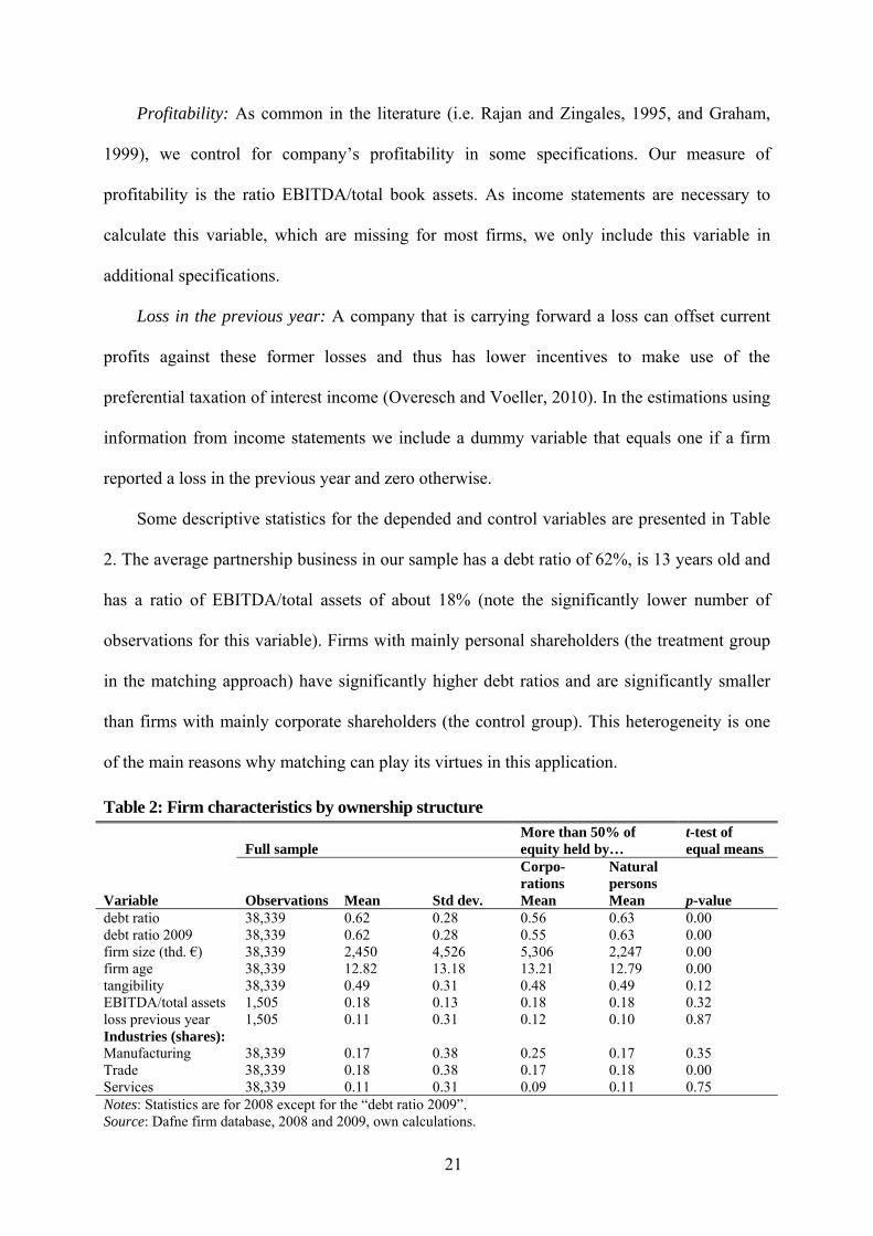
Some descriptive statistics for the depended and control variables are presented in Table
2. The average partnership business in our sample has a debt ratio of 62%, is 13 years old and
has a ratio of EBITDA/total assets of about 18% (note the significantly lower number of
observations for this variable). Firms with mainly personal shareholders (the treatment group
in the matching approach) have significantly higher debt ratios and are significantly smaller
than firms with mainly corporate shareholders (the control group). This heterogeneity is one
of the main reasons why matching can play its virtues in this application.
Table 2: Firm characteristics by ownership structure
Full sample More than 50% of equity held by…
t-test of equal means
Corpo-rations
Natural persons
Variable Observations Mean Std dev. Mean Mean p-value debt ratio 38,339 0.62 0.28 0.56 0.63 0.00 debt ratio 2009 38,339 0.62 0.28 0.55 0.63 0.00 firm size (thd. €) 38,339 2,450 4,526 5,306 2,247 0.00 firm age 38,339 12.82 13.18 13.21 12.79 0.00 tangibility 38,339 0.49 0.31 0.48 0.49 0.12 EBITDA/total assets 1,505 0.18 0.13 0.18 0.18 0.32 loss previous year 1,505 0.11 0.31 0.12 0.10 0.87 Industries (shares): Manufacturing 38,339 0.17 0.38 0.25 0.17 0.35 Trade 38,339 0.18 0.38 0.17 0.18 0.00 Services 38,339 0.11 0.31 0.09 0.11 0.75 Notes: Statistics are for 2008 except for the “debt ratio 2009”. Source: Dafne firm database, 2008 and 2009, own calculations.
22
Between 2008 and 2009, the mean debt ratio decreases slightly for firms where
corporations have the majority interest stake (the difference is significant at the 1% level), and
remains constant for firms with natural persons as the majority shareholders. This may
indicate that while there was a general trend towards a lower debt ratio in this time period,
presumably due to tighter credit conditions during the financial crisis, the firms in the
treatment group did not follow this trend and thus increased their debt ratio relative to the
control group. This is the expected direction of relative change in the debt ratios due to the
introduction of the final withholding tax. The following econometric analysis identifies a
causal effect and allows inference.
5 Empirical results
5.1 Matching quality
Before we report the results with respect to our research question, we first provide information
on the propensity score estimation and the matching quality. The results from the logistic
regression used to estimate the propensity score (see Table A-1 in the Appendix) reflect the
differences between firms with predominantly natural persons or corporations as shareholders,
as this distinction defines treatment and control groups. Firms in the treatment group, where
natural persons hold a majority interest stake, are smaller and slightly older on average and
have higher debt ratios than the firms in the control group, ceteris paribus. With respect to the
share of tangible assets, the groups do not differ significantly. Firms in the treatment group
are more often based in communities with lower local business tax rates. The industry
distribution differs between treatment and control groups as well. The significant differences
suggest that matching is important in this application to ensure that treatment and control
groups are sufficiently similar.

After having estimated the propensity score, we apply kernel matching to identify
suitable control observations for every firm in the treatment group. Imposing the common
support condition reduces the sample size only slightly, by 0.12%. To evaluate the matching
quality we refer to the standardized bias SBx for each variable in X, which is calculated as the
difference between the mean characteristic of the treated ( 1x ) and matched control firms ( 2x ),
standardized by the square root of the average of the variances in the two groups (Rosenbaum
and Rubin, 1985) and expressed as a percentage:
%
2
)(100
22
21
21 xx
x
xxSB
. (5)
After matching, SBx should not exceed about 5% for the key variables as a rule of thumb;
otherwise the mean difference is considered quite large and may indicate a lack of balancing
(Caliendo and Kopeinig, 2008). The standardized bias before and after kernel matching is
presented in Fehler! Ungültiger Eigenverweis auf Textmarke.. After matching the SBx
statistics are acceptable for all variables, in particular they are very low for the debt ratio and
the firm size, which exhibited large biases before matching. The mean absolute standardized
bias over all variables is below 5%, which indicates high matching quality.
Table 3: Standardized bias before and after matching Treatment group Control group Mean Mean Standardized bias in %
Variable Before matching
After matching
Before matching
After matching
local business tax rate 382% 384% 379% 4.12 4.99 debt ratio 0.63 0.56 0.63 25.23 - 1.12 log. firms size 6.83 7.69 6.84 61.37 - 0.67 log. firm age 2.12 2.16 2.09 3.78 4.08 tangibility 0.49 0.48 0.51 1.45 6.20 Industries (shares): Manufacturing 0.17 0.25 0.16 -20.36 1.42 Trade 0.18 0.17 0.17 1.98 1.79 Service 0.11 0.09 0.14 7.58 -7.28 Note: Statistics are for 2008. Source: Dafne firm database, 2008, own calculations.
23
24
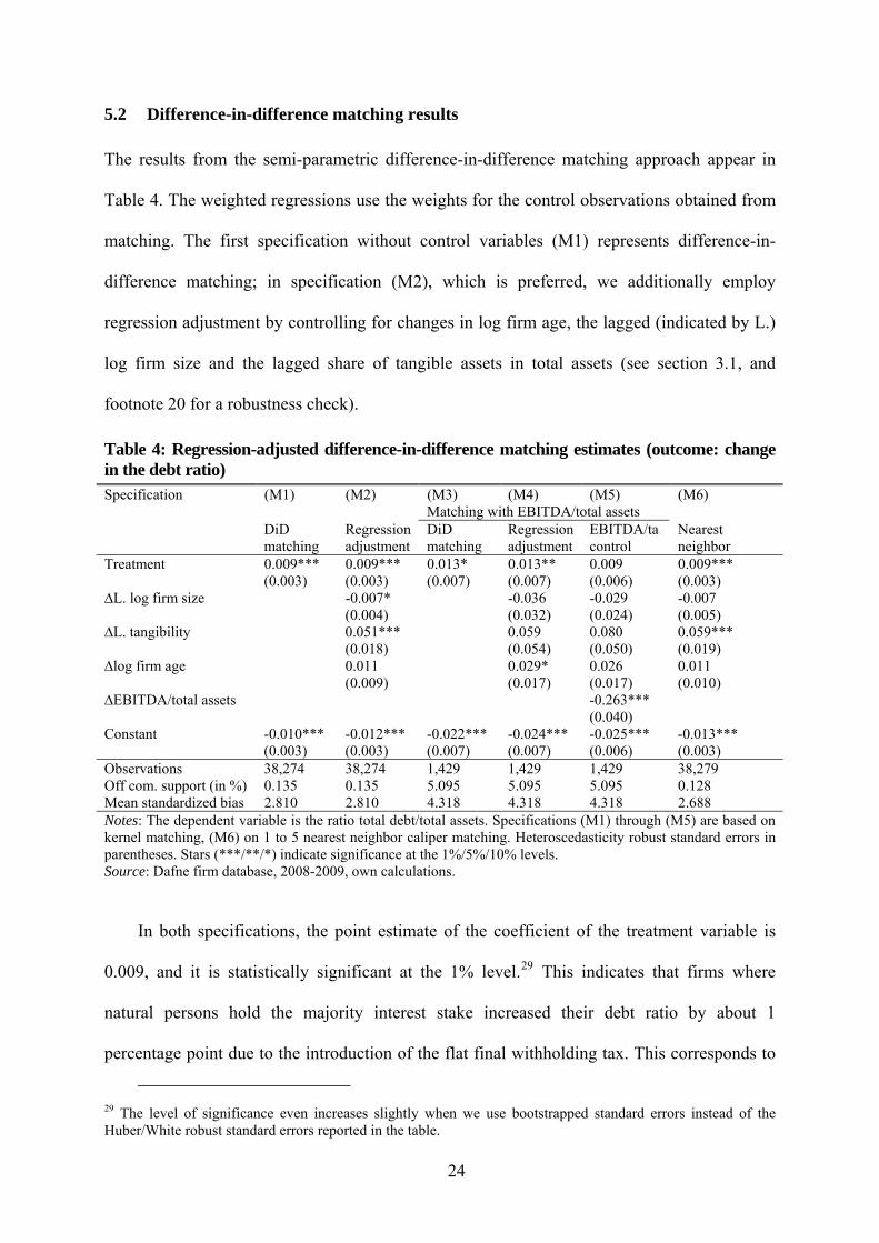
5.2 Difference-in-difference matching results
The results from the semi-parametric difference-in-difference matching approach appear in
Table 4. The weighted regressions use the weights for the control observations obtained from
matching. The first specification without control variables (M1) represents difference-in-
difference matching; in specification (M2), which is preferred, we additionally employ
regression adjustment by controlling for changes in log firm age, the lagged (indicated by L.)
log firm size and the lagged share of tangible assets in total assets (see section 3.1, and
footnote 20 for a robustness check).
Table 4: Regression-adjusted difference-in-difference matching estimates (outcome: change in the debt ratio) Specification (M1) (M2) (M3) (M4) (M5) (M6) Matching with EBITDA/total assets DiD
matching Regression adjustment
DiD matching
Regression adjustment
EBITDA/ta control
Nearest neighbor
Treatment 0.009*** 0.009*** 0.013* 0.013** 0.009 0.009*** (0.003) (0.003) (0.007) (0.007) (0.006) (0.003) ∆L. log firm size -0.007* -0.036 -0.029 -0.007 (0.004) (0.032) (0.024) (0.005) ∆L. tangibility 0.051*** 0.059 0.080 0.059*** (0.018) (0.054) (0.050) (0.019) ∆log firm age 0.011 0.029* 0.026 0.011 (0.009) (0.017) (0.017) (0.010) ∆EBITDA/total assets -0.263*** (0.040) Constant -0.010*** -0.012*** -0.022*** -0.024*** -0.025*** -0.013*** (0.003) (0.003) (0.007) (0.007) (0.006) (0.003) Observations 38,274 38,274 1,429 1,429 1,429 38,279 Off com. support (in %) 0.135 0.135 5.095 5.095 5.095 0.128 Mean standardized bias 2.810 2.810 4.318 4.318 4.318 2.688 Notes: The dependent variable is the ratio total debt/total assets. Specifications (M1) through (M5) are based on kernel matching, (M6) on 1 to 5 nearest neighbor caliper matching. Heteroscedasticity robust standard errors in parentheses. Stars (***/**/*) indicate significance at the 1%/5%/10% levels. Source: Dafne firm database, 2008-2009, own calculations.
In both specifications, the point estimate of the coefficient of the treatment variable is
0.009, and it is statistically significant at the 1% level.29 This indicates that firms where
natural persons hold the majority interest stake increased their debt ratio by about 1
percentage point due to the introduction of the flat final withholding tax. This corresponds to
29 The level of significance even increases slightly when we use bootstrapped standard errors instead of the Huber/White robust standard errors reported in the table.
25
an increase of 1.4% relative to the mean debt ratio in the treatment group of 63%. The
direction of the effect is consistent with our hypothesis. After the introduction of the flat final
withholding tax on interest income, personal shareholders can save taxes when investing in
the capital market instead of their own businesses, so they have an additional incentive to
finance their businesses with debt instead of equity. We discuss the effect size further in
section 5.4.
Specifications (M3), (M4), and (M5) provide robustness checks where we include the
ratio EBITDA/total assets, which captures profitability, as an additional variable in the set of
matching variables X. This reduces the sample size significantly, as profit and loss accounts
are not reported for most firms (as mentioned before). The standardized bias after matching
only changes marginally.30 Specification (M3) again is DiD matching without regression
adjustment, in specification (M4) we include the controls as in specification (M2), and in
specification (M5) we additionally use EBITDA/total assets in the regression adjustment. In
the three estimations, the point estimate of the coefficient of the treatment indicator remains
similar compared to the baseline specifications (M1) and (M2) (it lies within their confidence
intervals). It is significant in two of the three specifications, (M3) and (M4), although the
standard errors are much larger due to the strongly reduced sample size. As a further
sensitivity check, in specification (M6) we employ 1 to 5 nearest-neighbor caliper matching
instead of kernel matching (see section 3.1). The coefficient remains the same as in the
baseline estimations and is significant at the 1% level.
We also conduct placebo tests where we implement the same estimation approach as in
specifications (M1) and (M2), but act as if the reform had taken place in 2006 instead of 2009,
using the sample 2005-2006 instead of 2008-2009. We choose 2006 for the placebo test
because there were no other potentially relevant tax reforms in that year, whereas 2007 and
30 Results are available from the authors on request.
26
2008 saw the introduction of the rich tax (see footnote 7) and the CIT reform mentioned in
section 3.2. The coefficient of the placebo treatment dummy variable is not significantly
different from zero in both specifications (with and without regression adjustment), which is
reassuring as it indicates that there was no differential time trend between the treatment and
control groups.
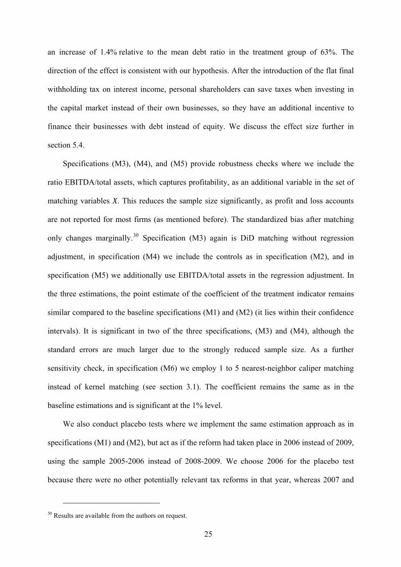
5.3 Structural approach
Table 5 shows the results from estimating the more structural equation (2) in first differences,
which includes the change in the tax rate differential between business income and interest
income as the key explanatory variable of interest; the dependent variable is the change in the
debt ratio. Specification (S1) uses data from 2008 and 2009, i.e. one year each before and
after the tax reform, while specification (S2) is based on the longer estimation period of 2004-
2009.31
We instrument the change in the tax rate differential with the change we would observe if
there had not been any modifications in the shareholder structure between 2007 and 2009 (see
section 3.2). As there are only few changes in the shareholder structure in the data, the
instrument is very strong, as indicated by the very large first stage F-statistics of the excluded
instrument and Shea’s Partial R2 at the bottom of the table. In specification (S2), we
additionally control for the change in the combined business tax rate to account for the
business tax reform of January 1, 2008, as mentioned before. The first stage statistics show
that the instrument for this control variable (which is analogous to the one just described) is
highly relevant as well.
The results from both specification show that a higher differential between the tax rate on
business income and the tax rate on interest income has a positive and significant effect on
31 We prefer specification (S1), as the wider time window might potentially take in more distortions from other events that the controls might not completely capture.
27
firms’ debt ratios with point estimates of 0.042 to 0.043. This indicates that a reduction of the
tax rate on interest income by 20 percentage points, while leaving the tax rate on business
income unchanged (which is similar to the introduction of the flat final withholding tax in
2009), increases the debt ratio by about 20*0.042 ≈ 0.84 percentage points for firms with
exclusively natural persons as shareholders, or 1.4% relative to the mean debt ratio of 62% in
the sample (the effect size is further discussed below).
Table 5: Results from IV estimations in first differences (dep. var.: change in the debt ratio) Specification (S1) (S2) Estimation period 2008-2009 2004-2009 ∆tax rate differential 0.042*** 0.043*** (0.012) (0.012) ∆L. tangibility 0.034*** 0.028*** (0.007) (0.005) ∆L. log firm size -0.007*** -0.008*** (0.002) (0.002) ∆log firm age 0.009*** 0.014*** (0.003) (0.003) ∆business income tax rate 0.123*** (0.040) year 2006 0.001 (0.017) year 2007 0.009* (0.005) year 2008 0.014*** (0.002) Constant -0.011*** -0.011*** (0.002) (0.002) Observations 38,339 62,769 1st stage F statistic (∆tax rate differential) 76,255 38,700 Shea’s Partial R2 (∆tax rate differential) 0.924 0.894 1st stage F stat. (∆business income tax rate) 8772 Shea’s Partial R2 (∆business income tax rate) 0.552 Notes: The dependent variable is the year-to-year change in the ratio total debt/total assets. ∆tax rate differential is the year-to-year difference in the tax rate differential between business and interest income. It is treated as endogenous; the simulated 1st differenced tax rate differential based on the twice-lagged ownership structure is used as the excluded instrument. ∆corporate tax rate is treated analogously. Heteroscedasticity robust standard errors in parentheses. Stars (***/**/*) indicate significance at the 1%/5%/10% levels. Source: Own calculations based on the financial accounts database Dafne 2004-2009.
We turn to the control variables next. The positive and significant coefficient of the tax
rate on business income in specification (S2) indicates that higher business income taxes
increase the debt ratio, as expected. This confirms that debt is used as a tax shield. Decreasing
the business income tax rate by 10 percentage points (which is similar to the business tax
reform of January 2008) increases the debt ratio by 1.3 percentage points.
28
The share of tangible assets in total assets (tangibility) has a positive and significant
coefficient in both specifications. A higher liquidation value of a firm seems to support the
use of debt, presumably due to better credit conditions; this effect seems to outweigh the
effect of higher depreciation allowances, which should reduce the incentive to use debt as a
tax shield. The coefficient for firm size has a negative sign, which is in line with the view that
larger firms, which are subject to stricter publication rules, find it easier to issue equity. For
the age of the firms, we expected a negative coefficient as older firms should have lower debt
ratios based on the lifecycle hypothesis, but this is not confirmed. A possible explanation for
the positive effect of age on the debt ratio could be that older firms have favorable credit
conditions because of their long-standing relationships with banks.
In specifications (S1) and (S2), tangibility and firm size enter equation (2) in lagged
form. As the first differences of these lagged variables may still be endogenous in the first
differenced equation, we conduct robustness checks with respect to these control variables
(see Table A-2 in the Appendix). Based on the 2008-2009 data, specification (S3) includes the
twice-lagged levels of the two variables in the first differenced equation, whereas (S4)
includes the contemporaneous first differences, but treats them as endogenous and uses the
twice-lagged levels as their instruments. Specifications (S6) and (S7) are analogous, but are
based on the longer observation period of 2004-2009. The point estimates obtained are
somewhat smaller, but not significantly different from the baseline estimates, so we conclude
that these are robust.
In specifications (S5) (for the short time window) and (S8) (for the longer time window),
we include two additional control variables in equation (2) to account for differences in
profitability: the ratio EBITDA/total assets and a dummy variable indicating if a firm reported
a loss in the previous year. Here our samples size shrinks significantly due to missing income
statements. Since EBITDA/total assets might be endogenous with respect to the finance
structure, we use its twice lagged level as instrument for the first differenced control variable.

29
Although this time the point estimates of the coefficient of the tax rate differential increase in
comparison to the baseline estimates, they are not significantly different, which again
confirms robustness. In a further robustness check we exploit international variation in global
ultimate ownership and find consistent results (Appendix B).
5.4 Discussion of the effect size
To assess if the results from the structural approach are consistent with those from the
difference-in-difference matching approach, we compare the estimated average effects of the
introduction of the flat tax on capital income in Germany in 2009. In the matching model, the
change in the debt ratio for the treated firms is given by the estimated coefficient, which
represents the treatment effect on the treated (0.9 percentage points in the baseline
estimations), while for the control observations it is zero. To obtain the mean change in the
debt ratio over all firms, we weight these effects by the shares of both groups in the sample
and obtain a weighted average increase in the debt ratio of 0.8 percentage points.
For the more structural approach the mean change in the debt ratio is calculated by
multiplying the estimated coefficient of the tax rate differential, i.e. 0.042 in the baseline
specification, with the mean change in this differential due to the introduction of the flat
withholding tax, which is 16.66%; this change is smaller than the nominal reduction of the tax
rate on interest income because of the weighs jit in equation (3), which reflect that only
natural persons as shareholders benefit from the tax reform. Thus, the mean increase in the
debt ratio in the sample due to the reform amounts to 0.74 percentage points based on this
approach.32
We conclude that both the matching and the structural approaches provide consistent
results, as the point estimates are similar and statistically not significantly different from each
32 It is unlikely that the local treatment effect identified in our IV estimation differs from the global effect because of the few changes in the shareholder structure.

30
other. A methodological implication beyond this application is that we validate the general
structural model with a semi-parametric event study: If the structural model were
misspecified, the estimate would be expected to be biased, while the matching estimate would
still be consistent; in this case, we would expect a significant difference between the two
estimates.
Our estimate from the structural model can be compared with the results from the
literature mentioned in the introduction to a limited extent. Alworth and Arachi (2001, Table
7) regress the change of the debt ratio on the level of a composite term of the tax rates on
interest income, dividends and capital gains. Their estimated coefficient of 0.034 implies that
a reduction of 20 percentage points in the tax rate on interest income leads to an increase of
the debt ratio by 0.68 percentage points every year, somewhat less than our estimated one-
time change of 0.84 percentage points. Their estimated ratio of the coefficients of the tax rates
on corporate income and on interest income is about 3 to 1, similar to our estimated ratio
(0.123 to 0.042).
Comparability with Graham (1999, Table 6) is limited because he uses debt to market
value as the dependent variable. Our result can best be related to one of his estimations, where
he uses the corporate tax rate and the personal tax penalty, i.e. a composite term of the tax
rates on interest income, dividends and capital gains, as separate independent variables. His
estimated coefficient for the composite term is -0.219; thus, a 20 percentage-points reduction
in the tax rate on interest income leads to an increase in the debt to market value of more than
4 percentage points, which is a much larger response than ours. As Graham runs this OLS
regression on a 1994 cross-section of data without accounting for firm-specific effects, a bias
in this estimate cannot be ruled out. Overesch and Voeller (2010, Table 4), who use the same
definition of the debt ratio as the dependent variable as we do, also estimate a much larger
coefficient for the tax rate on interest income of -0.56. However, the standard error of their
estimate of 0.27 is so large that our much more precisely estimated coefficient of the tax rate

31
differential of 0.042 is still included in their 95% confidence interval (the sign must be
switched for comparison because the tax rate on interest income is subtracted in our
differential). Note that these three studies rely on completely different identification strategies
than this paper (i.e. cross-country variation in tax codes or firms’ payout policies) and on data
for different countries.
Our estimated increase in the debt ratio by 1.4% in relative terms due the introduction of
the final withholding tax may seem quite small, given the strong incentives. A possible
explanation for the small reaction could be that some firms are financially constrained. As
mentioned, even before the tax reform, debt finance was tax favored (like in most other
countries), as it can be used as a tax shield due to the deduction of interest payments from the
tax base. Firms may thus have exploited this by increasing their debt ratios as much as
possible prior to and independent of the reform being implemented. If their optimization led
them into a corner solution before the reform, i.e. they could not increase their debt further
due to finance constraints, it is clear that they could not react to the additional incentive to use
debt introduced with the final withholding tax. This explanation seems especially plausible as
the tax reform was implemented during the financial crisis, when firms may have had
problems to obtain additional debt finance. Furthermore, we are measuring short-term effects.
If adjustment of the finance structure takes more than a year of time, we are not capturing the
full long-term effects. In the next section, we investigate effect heterogeneity, which provides
some support for these explanations.
5.5 Heterogeneous effects
We use variants of the baseline specification (S1) to investigate differences in the
responsiveness of the debt ratio to the tax rate differential by different types of firms (Table
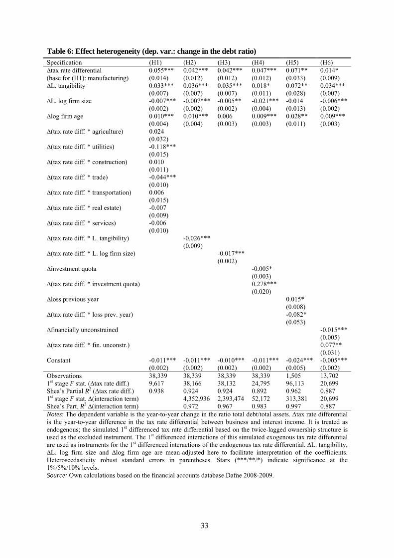
6). In specification (H1), we are interested in effect heterogeneity between industry classes.
To analyze these differences we include interaction terms of the tax rate differential with
32
dummy variables indicating that a firm belongs to i) agriculture, forestry, fishery, mining and
quarrying; ii) utilities; iii) construction; iv) trade; v) transportation, storage, information and
communication; vi) real estate and renting; and vii) services.33 The manufacturing sector
constitutes the base category. For the manufacturing sector, the estimated coefficient of the
tax rate differential is 0.055 and significant; this is a larger point estimate than that from the
pooled estimation (0.042). Firms active in utilities and trade exhibit significantly weaker
responses than manufacturing firms; perhaps for these industries, non-tax determinants of the
debt ratio are relatively more important. For the highly regulated and oligopolistic utilities
industry, the effect even goes in the other direction.
In specification (H2), we investigate whether firms with higher tangibility – and thus
higher depreciation allowances and a higher non-debt tax shield – respond less to the tax rate
differential. The results confirm this hypothesis, as the estimated coefficient of the interaction
term between the tax rate differential and the mean-adjusted firms’ tangibility is negative and
significant.
In specification (H3) we analyze whether the size of the firm matters for the debt
adjustment. A priori we had no clear expectation of the sign of the interaction term. On the
one hand, larger firms could react more strongly as adjusting the finance structure might
involve some fix costs, e.g. bank negotiations, such that only for large firms the tax benefit
exceeds the fixed adjustment costs. On the other hand, it is also possible that smaller firms are
more responsive, since personal shareholders, who benefit from the tax reform, may have
more influence on the finance structure of smaller firms due to their smaller number and
closer relationship to the firm. The estimated negative coefficient between the mean-adjusted
firm size and the tax rate differential suggests that the latter mechanism dominates.
33 As the change in the tax rate differential is treated as endogenous in the IV estimation, changes in its interaction terms are also endogenous. Therefore, the changes in the interactions of the IV for the tax rate differential are used as additional instruments. First stage statistics for the changes in the industry dummy interactions are satisfactory. They are not shown for brevity, but available from the authors on request. First stage statistics for the other specifications are provided at the bottom of the table.
33
Table 6: Effect heterogeneity (dep. var.: change in the debt ratio) Specification (H1) (H2) (H3) (H4) (H5) (H6) ∆tax rate differential 0.055*** 0.042*** 0.042*** 0.047*** 0.071** 0.014* (base for (H1): manufacturing) (0.014) (0.012) (0.012) (0.012) (0.033) (0.009) ∆L. tangibility 0.033*** 0.036*** 0.035*** 0.018* 0.072** 0.034*** (0.007) (0.007) (0.007) (0.011) (0.028) (0.007) ∆L. log firm size -0.007*** -0.007*** -0.005** -0.021*** -0.014 -0.006*** (0.002) (0.002) (0.002) (0.004) (0.013) (0.002) ∆log firm age 0.010*** 0.010*** 0.006 0.009*** 0.028** 0.009*** (0.004) (0.004) (0.003) (0.003) (0.011) (0.003) ∆(tax rate diff. * agriculture) 0.024 (0.032) ∆(tax rate diff. * utilities) -0.118*** (0.015) ∆(tax rate diff. * construction) 0.010 (0.011) ∆(tax rate diff. * trade) -0.044*** (0.010) ∆(tax rate diff. * transportation) 0.006 (0.015) ∆(tax rate diff. * real estate) -0.007 (0.009) ∆(tax rate diff. * services) -0.006 (0.010) ∆(tax rate diff. * L. tangibility) -0.026*** (0.009) ∆(tax rate diff. * L. log firm size) -0.017*** (0.002) ∆investment quota -0.005* (0.003) ∆(tax rate diff. * investment quota) 0.278*** (0.020) ∆loss previous year 0.015* (0.008) ∆(tax rate diff. * loss prev. year) -0.082* (0.053) ∆financially unconstrained -0.015*** (0.005) ∆(tax rate diff. * fin. unconstr.) 0.077** (0.031) Constant -0.011*** -0.011*** -0.010*** -0.011*** -0.024*** -0.005*** (0.002) (0.002) (0.002) (0.002) (0.005) (0.002) Observations 38,339 38,339 38,339 38,339 1,505 13,702 1st stage F stat. (∆tax rate diff.) 9,617 38,166 38,132 24,795 96,113 20,699 Shea’s Partial R2 (∆tax rate diff.) 0.938 0.924 0.924 0.892 0.962 0.887 1st stage F stat. ∆(interaction term) 4,352,936 2,393,474 52,172 313,381 20,699 Shea’s Part. R2 ∆(interaction term) 0.972 0.967 0.983 0.997 0.887 Notes: The dependent variable is the year-to-year change in the ratio total debt/total assets. ∆tax rate differential is the year-to-year difference in the tax rate differential between business and interest income. It is treated as endogenous; the simulated 1st differenced tax rate differential based on the twice-lagged ownership structure is used as the excluded instrument. The 1st differenced interactions of this simulated exogenous tax rate differential are used as instruments for the 1st differenced interactions of the endogenous tax rate differential. ∆L. tangibility, ∆L. log firm size and ∆log firm age are mean-adjusted here to facilitate interpretation of the coefficients. Heteroscedasticity robust standard errors in parentheses. Stars (***/**/*) indicate significance at the 1%/5%/10% levels. Source: Own calculations based on the financial accounts database Dafne 2008-2009.
34
It is possible that firms adjust their debt ratio primarily when they invest by financing the
investment predominantly by debt or equity. In specification (H4) we test this hypothesis by
including the mean-adjusted investment quota (defined as the ratio of the change in tangible
book assets/beginning-of-period stock of tangible book assets) and its interaction with the tax
rate differential. The results confirm the hypothesis that firms investing more also adjust their
capital structure more. As the investment quota is mean-adjusted, a firm with the mean
investment quota (which is 10% in our sample) has a coefficient of the tax rate differential of
0.047. If a firm’s investment quota is ten percentage points higher, the effect of the tax rate
differential is 0.1 * 0.278 = 0.0278 higher and thus amounts in total to 0.075. This may
suggest that the long-term effect of the introduction of the final withholding tax will be larger
than the estimated short-term effect, as firms subsequently invest over time and then may
simultaneously adjust their debt ratios.34
In specification (H5), we analyze whether firms that are carrying forward a loss respond
less to a change in the tax rate differential, as one would expect as these firms have reduced
tax incentives. The estimated coefficient of the interaction term between the dummy variable
indicating a loss in the previous year and the tax rate differential is significantly negative
indeed and amounts to -0.082. Consistently, the point estimate for the tax rate differential’s
coefficient for the remaining firms increases to 0.071. Thus firms that are carrying forward a
loss do not respond to the incentive created by the tax rate differential.
In the last specification (H6), we check whether financially unconstrained firms react
more strongly to a change in the tax rate differential. Similarly to van Binsbergen et al.
(2010), we classify those firms as financially unconstrained if the debt issuance or debt
reduction scaled by total assets exceeds the 66th percentile or if the equity issuance or
34 Since investment might be endogenous, we additionally use an IV approach to assess robustness. As the excluded instrument for an individual firm’s investment quota, we use the average investment quota of all firms within the same 3-digit industry (without the firm’s own investment quota). The coefficient of the interaction term is positive and significant again (0.925 with a standard error of 0.268). We report the OLS results in the table because the first stage statistics do not sufficiently support the strength of the instrument for investment.
35
reduction exceeds the 66th percentile. The estimated coefficient of the interaction term
between the dummy variable indicating a financially unconstrained firm and the tax rate
differential is 0.077 and significant. Thus, for unconstrained firms the effect of the tax rate
differential adds up to 0.091 (0.077 + 0.014), which is more than double the size of the
baseline estimate. This suggests that financially unconstrained firms indeed adjust their debt
ratios much more after tax changes than constrained firms, and that the small size of the
average effect is partly due to constrained firms, which cannot further increase their debt
ratios.
6 Conclusion
Various countries have implemented, or are considering implementing, flat rate taxes on
interest income. Typically the tax rate on interest income is low in comparison to marginal tax
rates on income generated by unincorporated businesses, as the latter type of income is subject
to a progressive personal income tax. The resulting tax rate differential creates additional
incentives to increase leverage, as business owners save taxes if they finance their business
with debt rather than equity and invest their funds in the capital market instead, e.g. the
banking system, where returns are taxed at the low tax rate on interest income. To estimate
how much firms adjust their behavior by increasing their debt usage due to these tax
incentives, we exploit the introduction of a flat final withholding tax in Germany in 2009 as a
quasi-experiment. This policy reform reduced the tax rate on interest income by 18 percentage
points. We use individual firm level panel data to identify the effect on the debt ratio.
In line with the hypothesis, the results from a difference-in-difference matching approach
indicate that partnership firms, where personal shareholders hold a majority equity stake,
increased their debt ratios (total liabilities/total assets) by 1.4% due to the introduction of the
final withholding tax. As our paper shows, this finding is consistent with the results from a
more structural approach where the debt ratio is modeled as a function of the tax rate

36
differential. The coefficient of the tax rate differential implies that a reduction of the tax rate
on interest income by 10 percentage points increases the debt ratio by 0.42 percentage points.
We find larger effects for smaller firms, firms that invest, firms not carrying forward a loss
from the previous year, and firms that do not appear to be financially constrained.
The rather small reaction of firms’ debt usage suggests that even a significant differential
between the tax rates on business and interest income does not seem to cause large distortions
through behavioral adjustment. Therefore, a flat tax on interest income, which can be
implemented comparably simply as a final withholding tax, may be a viable alternative to a
Dual Income Tax, which may be conceptually more appealing due to the equal treatment of
equity and debt, but which is more complicated to implement.
We estimate short-term effects within one year after the implementation of the tax
reform. It is possible that long-term effects are larger, as our analysis of heterogeneous effects
suggests that firms do not completely adjust their financial structure immediately, but rather
gradually when they decide how to finance new investment, and as during the financial crisis
credit may have been hard to obtain. Subsequent research should therefore be directed
towards estimating long-term effects. Another important avenue for future research is to
investigate how taxes on interest income affect investment behavior.

37
References
Almeida, Heitor and Murillo Campello (2007): Financial constraints, asset tangibility, and
corporate investment, Review of Financial Studies, 20(5), 1429-1460.
Alworth, Julian and Giampaolo Arachi (2001): The effect of taxes on corporate financing
decision: Evidence from a panel of Italien firms, International Tax and Public Finance, 8,
353-376.
Auerbach, Alan J. (2002): Taxation and corporate financial policy, in Alan Auerbach and
Martin Feldstein (eds), Handbook of Public Economics 3, Amsterdam: Elsevier North-
Holland, 1251-1292.
Austan Goolsbee (1998): Taxes, organizational form, and the deadweight loss of the corporate
income tax, Journal of Public Economics, 6, 143-152.
Austan Goolsbee (2004): The impact of corporate income tax: Evidence from state
organizational data, Journal of Public Economics, 88, 2283-2299.
Bach, Stefan and Frank Fossen (2008): Reforming the German local business tax – Lessons
from an international comparison and a microsimulation analysis, FinanzArchiv–Public
Finance Analysis, 64(2), 245-272.
Bang, Heejung and James Robbins (2005): Doubly robust estimation in missing data and
causal inference models, Biometrics, 61(4), 962-972
Buettner, Thiess (2006): The incentive effect of fiscal equalization transfers on tax policy,
Journal of Public Economics, 90, 477-497.
Caliendo, Marco and Sabine Kopeinig (2008): Some practical guidance for the
implementation of propensity score matching, Journal for Economic Surveys, 22(1), 31-
72.
Caliendo, Marco and Steffen Künn (2011): Start-up subsidies for the unemployed: Long-term
evidence and effect heterogeneity, Journal of Public Economics, 95(3-4), 311-331.

38
Cameron, A. Colin and Pravin K. Trivedi (2006): Microeconometrics, methods and
applications, Cambridge, UK: Cambridge University Press.
Chan, Howard, Robert Faff and Alan Ramsay (2005): Firm size and information content of
annual earnings announcements: Australian evidence, Journal of Business Finance and
Accounting, 32, 211-253.
Chetty, Ray and Emmanuel Saez (2006): The effects of the 2003 dividend tax cut on
corporate behavior: Interpreting the evidence, American Economic Review, 96(2), 124-
129.
DeAngelo, Harry, Linda DeAngelo and René M. Stulz (2006): Dividend policy and the
earned/contributed capital mix: A test of the life-cycle theory, Journal of Financial
Economics, 81 (2), 227-254.
DeAngelo, Harry and Ronald W. Masulis (1980): Optimal capital structure under taxation,
Journal of Financial Economics, 8, 3-29.
Devereux, Michael P., Ben Lockwood and Michela Redoano (2008): Do countries compete
over corporate tax rates? Journal of Public Economics, 92(5-6), 1210-1235.
Dwenger, Nadja and Viktor Steiner (2009): Financial leverage and corporate taxation:
Evidence from German corporate tax return data, DIW Discussion Paper 855, German
Institute for Economic Research.
Egger, Peter, Marko Koethenbuerger and Michael Smart (2010): Do fiscal transfers alleviate
business tax competition? Evidence from Germany, Journal of Public Economics, 94,
235-246.
Fazzari, Steven M., R. Glenn Hubbard and Bruce C. Petersen (1988): Financing constraints
and corporate investment, Brookings Papers on Economic Activity, 19(1), 141-195
Fazzari, Steven M., R. Glenn Hubbard and Bruce C. Petersen (2000):
Investment-cash flow sensitivities are useful: A comment on Kaplan and Zingales,
Quarterly Journal of Economics, 115(2), 695-705.

39
Federal Ministry of Finance (2006–2011): Die wichtigsten Steuern im internationalen
Vergleich (The most important taxes in international comparison), Berlin, Germany.
Federal Statistical Office (2011): Umsatzsteuerstatistik 2009 (VAT statistics 2009),
Wiesbaden, Germany.
Fuest, Clemens and Alfons Weichenrieder (2002): Tax competition and profit shifting: On the
relationship between personal and corporate tax rates, IFO-Studien, 48, 611-632.
Fuest, Clemens, Bernd Huber and Soren B. Nielson (2002): Why is the corporate tax rate
lower than the personal tax rate? The role of new firms, Journal of Public Economics, 87,
157-174.
Goolsbee, Austan (1998): Taxes, organizational form, and the deadweight loss of the
corporate income tax, Journal of Public Economics, 69, 143-152.
Goolsbee, Austan (2004): The impact of the corporate income tax: Evidence from state
organizational form data, Journal of Public Economics, 88, 2283-2299.
Gordon, Roger H. and Jeffrey K. MacKie-Mason (1990): Effects of the Tax Reform Act of
1986 on corporate financial policy and organizational form, in Joel Slemrod (ed.), Do
taxes matter? Cambridge: MIT Press, 91-131.
Gordon, Roger H. and Jeffrey K. MacKie-Mason (1994): Tax distortions to the choice of
organizational form, Journal of Public Economics, 55(2), 279-306.
Graham, John R. (1999): Do personal taxes affect corporate financing decisions? Journal of
Public Economics, 73, 147-185.
Graham, John R. (2003): Taxes and corporate finance: A review, Review of Financial Studies,
16, 1075-1129.
Gruber, Jon and Emmanuel Saez (2002): The elasticity of taxable income: Evidence and
implications, Journal of Public Economics, 84(1), 1-32.
Harris, Milton and Artur Raviv (1990): The theory of capital structure, Journal of Finance,
46, 297-355.

40
Heckman, James, Hidehiko Ichimura and Petra E. Todd (1997): Matching as an econometric
evaluation estimator: Evidence from evaluating a job training programme, Review of
Economic Studies, 64(4), 605-654.
Jacob, Marcus and Martin Jacob (2011): Taxation, dividends and share repurchases: Taking
evidence global, working paper available at SSRN: http://ssrn.com/abstract=1532674, last
accessed February 14, 2012.
Miller, Merton H. (1977): Debt and taxes, Journal of Finance, 32(2), 261-275.
OECD (2007): OECD economic surveys: Spain, 2007(1), Paris: OECD Publishing.
OECD (2011): OECD tax database,
http://www.oecd.org/document/60/0,3746,en_2649_34533_1942460_1_1_1_1,00.html,
last accessed January 22, 2012.
Overesch, Michael and Dennis Voeller (2010): The impact of personal and corporate taxation
on capital structure choices, Finanzarchiv–Public Finance Analysis, 66(3), 263-294.
Public Finances General Directorate (2009): The French tax system, situation as at 31. August
2009, Tax Policy Directorate,
http://www.impots.gouv.fr/portal/deploiement/p1/fichedescriptive_1006/fichedescriptive_
1006.pdf, last accessed January 23, 2012.
Rajan, Raghuram G. and Luigi Zingales (1995): What do we know about capital structure?
Some evidence from international data, Journal of Finance, 50, 1421-1460.
Rosenbaum, Paul R. and Donald B. Rubin (1985): Constructing a control group using
multivariate matched sampling methods that incorporate the propensity score, American
Statistician, 39, 33-38.
Smith, Jeffrey A. and Petra E. Todd (2005): Does matching overcome LaLonde’s critique of
nonexperimental estimators? Journal of Econometrics, 125(1-2), 305-353.
Statistical Offices of the Federation and the States (2004-2009): Statistik local (Local
statistics), Wiesbaden, Germany.

41
Stuart, Elizabeth A. (2010): Matching methods for causal inference: A review and a look
forward, Statistical Science, 25(1), 1-21.
Thoresen, Thor O. and Annette Alstadsaeter (2008): Shifts in organizational form under a
Dual Income Tax system, FinanzArchiv–Public Finance Analysis 66(4), 384-418.
Van Binsbergen, Jules H., John Graham and Jie Yang (2010): The cost of debt, NBER
Working Paper 16023, National Bureau of Economic Research.

42
Appendix A: Supplementary estimation results
Table A-1: Logistic regression of the propensity score (2008 data) Logit coefficient Std error local business tax rate -0.126*** (0.041) debt ratio 1.125*** (0.077) log firm size -0.495*** (0.017) log firm age 0.142*** (0.024) tangibility 0.122 (0.087) Industry dummy variables for: agriculture, forestry and fishing 0.834*** (0.312) mining and quarrying -0.937*** (0.221) manufacturing 0.261* (0.138) electricity and gas supply -0.018 (0.165) water supply -0.812*** (0.199) construction 1.133*** (0.159) wholesale and retail trade 0.537*** (0.140) transportation and storage 0.075 (0.155) information and communication -0.695*** (0.183) accommodation and food service activities 0.469** (0.215) real estate activities 1.225*** (0.140) professional, scientific and technical activities 1.015*** (0.147) administrative and support service activities 0.440*** (0.168) public administration and defense 0.753 (0.758) human health and social work activities -0.149 (0.233) Constant 5.094*** (0.239) Observations 38,339 Pseudo R2 0.093 Notes: The dependent variable is the treatment indicator. It equals one for firms with more than half of their equity held by personal shareholders and zero otherwise. Stars (***/**/*) indicate significance at the 1%/5%/10% levels. Source: Dafne 2008, own calculations.

43
Table A-2: Additional robustness checks (dep. var.: change in the debt ratio) Specification (S3) (S4) (S5) (S6) (S7) (S8) Estimation period 2008-2009 2004-2009 Treatment of control variables Twice
lagged levels as controls
Endoge-nous controls (with IV)
Incl. profita-bility (with IV)
Twice lagged levels as controls
Endoge-nous controls (with IV)
Incl. profita-bility (with IV)
∆tax rate differential 0.031** 0.035*** 0.054* 0.030** 0.031** 0.056* (0.012) (0.013) (0.031) (0.013) (0.014) (0.031) ∆L. tangibility 0.089*** 0.050* (0.029) (0.030) ∆L. log firm size -0.009 -0.015* (0.013) (0.009) ∆log firm age 0.006* -0.003 0.021 0.011*** -0.003 0.027** (0.004) (0.004) (0.013) (0.003) (0.004) (0.011) ∆corporate income tax rate 0.089** 0.041 0.076 (0.041) (0.032) (0.070) L2. tangibility -0.004** -0.007*** (0.002) (0.001) L2. log firm size -0.002*** -0.003*** (0.000) (0.000) ∆tangibility 0.209*** 0.269*** (0.056) (0.044) ∆log firm size 0.213*** 0.306*** (0.038) (0.043) ∆EBITDA/total assets -0.272*** -0.255*** (0.082) (0.072) ∆loss previous year 0.018** 0.015*** (0.008) (0.005) year 2006 0.006 0.010 0.082** (0.021) (0.024) (0.040) year 2007 0.007 -0.001 0.022*** (0.005) (0.005) (0.008) year 2008 0.011*** 0.005* 0.020*** (0.002) (0.003) (0.006) Constant 0.010** -0.005* -0.027*** 0.013*** -0.003 -0.027*** (0.004) (0.002) (0.005) (0.003) (0.003) (0.005) Observations 38,339 38,339 1,505 62,771 62,768 3,264 1st stage F stat. (∆tax rate diff.) 70,916 33,637 57,200 37,944 28,759 36,738 Shea’s P. R2 (∆tax rate diff.) 0.922 0.913 0.957 0.889 0.921 0.938 1st stage F statistic (∆tangibility) 24 19 Shea’s Partial R2 (∆tangibility) 0.004 0.003 1st stage F stat. (∆log firm size) 225 274 Shea’s Partial R2 (∆log firm size) 0.011 0.014 1st st. F stat. (∆EBITDA/tot. asts) 34 40 Shea’s P. R2 (∆EBITDA/tot. asts) 0.080 0.063 1st stage F statistic (∆CIT rate) 8655 8672 3151 Shea’s Partial R2 (∆CIT rate) 0.552 0.550 0.648 Notes: The dependent variable is the year-to-year change in the ratio total debt/total assets. ∆tax rate differential is the year-to-year difference in the tax rate differential between business and interest income. It is treated as endogenous; the simulated 1st differenced tax rate differential based on the twice-lagged ownership structure is used as the excluded instrument. ∆corporate tax rate is treated analogously. In specifications (S4) and (S7) ∆L. tangibility and ∆L. log firm size and in (S5) and (S8) ∆EBITDA/total assets are instrumented with the twice lagged levels. Heteroscedasticity robust standard errors in parentheses. Stars (***/**/*) indicate significance at the 1%/5%/10% levels. Source: Own calculations based on the financial accounts database Dafne 2003-2009.

44
Appendix B: Global ultimate owners
In this paper, we use firms’ immediate shareholder structures in our identification strategy.
One might argue that ultimate ownership matters; several companies may be stringed between
the firm and the ultimate owner in the ownership chain. Therefore, in a robustness check we
exploit international variation in global ultimate ownership and use an identification strategy
similar to that of Overesch and Voeller (2010). This approach makes use of the fact that
different global owners face different tax rates for interest income. Besides Germany in 2009,
France and Spain also significantly changed their taxes on interest income in 2007 and 2008.
Spain introduced a flat tax on capital income on January 1, 2007. Interest income from
instruments with a maturity of less than one year, which was taxed progressively as general
income before the reform (tax rate: between 15 and 45%), is taxed with a flat rate of 18% now
(OECD, 2007, p. 113). France implemented an optional flat tax on interest income with a rate
of 18% on January 1, 2008 (Public Finance General Directorate, 2009). Before the reform,
interest income was taxed as general income with a rate between 5.5% and 40%.
In our data, for many firms we observe the type and country of residence of the global
ultimate owner, who is defined as the ultimate shareholder who directly or indirectly holds
more than 50% of a firm’s equity. Using the sub-sample of firms with a natural person as the
global ultimate owner, we regress the debt ratio on the tax rate on interest income faced by
this ultimate owner and the control variables used before, again in first differences to account
for time-invariant firm effects.35 International interest tax rates are derived from publications
by the German Federal Ministry of Finance (2006-2011). Because of the potential
endogeneity of the ownership structure, we again apply an IV estimation; as the excluded
instrument we use the interest tax rate which would have prevailed if the location of the global
35 For comparability with the results presented above we only include unincorporated businesses in the sample. Furthermore, we only consider shareholders from countries where sufficient observations are present, i.e. Belgium, Cyprus, Czech Republic, Denmark, Finland, France, Great Britain, Greece, Germany, Ireland, Italy, Japan, Luxemburg, Netherlands, Norway, Poland, Spain, Sweden, Switzerland, and the United States.
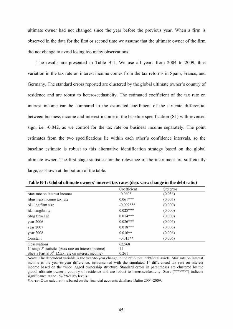
45
ultimate owner had not changed since the year before the previous year. When a firm is
observed in the data for the first or second time we assume that the ultimate owner of the firm
did not change to avoid losing too many observations.
The results are presented in Table B-1. We use all years from 2004 to 2009, thus
variation in the tax rate on interest income comes from the tax reforms in Spain, France, and
Germany. The standard errors reported are clustered by the global ultimate owner’s country of
residence and are robust to heteroscedasticity. The estimated coefficient of the tax rate on
interest income can be compared to the estimated coefficient of the tax rate differential
between business income and interest income in the baseline specification (S1) with reversed
sign, i.e. -0.042, as we control for the tax rate on business income separately. The point
estimates from the two specifications lie within each other’s confidence intervals, so the
baseline estimate is robust to this alternative identification strategy based on the global
ultimate owner. The first stage statistics for the relevance of the instrument are sufficiently
large, as shown at the bottom of the table.
Table B-1: Global ultimate owners’ interest tax rates (dep. var.: change in the debt ratio) Coefficient Std error ∆tax rate on interest income -0.060* (0.036)
∆business income tax rate 0.061*** (0.003)
∆L. log firm size -0.009*** (0.000)
∆L. tangibility 0.028*** (0.000)
∆log firm age 0.014*** (0.000)
year 2006 0.026*** (0.006)
year 2007 0.018*** (0.006)
year 2008 0.016** (0.006)
Constant -0.015** (0.006)
Observations 62,568 1st stage F statistic (∆tax rate on interest income) 11 Shea’s Partial R2 (∆tax rate on interest income) 0.261 Notes: The dependent variable is the year-to-year change in the ratio total debt/total assets. ∆tax rate on interest income is the year-to-year difference, instrumented with the simulated 1st differenced tax rate on interest income based on the twice lagged ownership structure. Standard errors in parentheses are clustered by the global ultimate owner’s country of residence and are robust to heteroscedasticity. Stars (***/**/*) indicate significance at the 1%/5%/10% levels. Source: Own calculations based on the financial accounts database Dafne 2004-2009.