Embed Size (px)
Citation preview
Business Complexity and Risk Management: Evidence fromOperational Risk Events in U.S. Bank Holding Companies∗
Anna Chernobai† Ali Ozdagli‡ Jianlin Wang§
September 2016
Abstract
Recent regulatory proposals tie the systemic importance of a financial institution to itscomplexity. However, we know little about how complexity affects a bank’s behavior, in-cluding its risk management. Using the gradual deregulation of banks’ nonbank activitiesduring 1996–1999 as a natural experiment, we show that the frequency and magnitude ofoperational risk events in U.S. bank holding companies have increased significantly with theirbusiness complexity. This trend is particularly strong for banks that were bound by regu-lations beforehand, especially for those with an existing Section 20 subsidiary, and weakerfor the other banks that were not bound and for nonbank financial institutions that werenot subject to the same regulations to begin with. These results reveal the darker side ofpost-deregulation diversification, which in earlier studies has been shown to lead to improvedstock and earnings performance. We use operational risk events as a risk management mea-sure because (i) the timing of the origin of each event is well identified, and can be yearsbefore it is materialized into a loss in the balance sheet, and (ii) the risk events can serveas a direct measure of materialized failures in risk management without being influencedby the confounding factors that drive asset prices, such as implicit government guarantees.Our findings have important implications for the regulation of financial institutions deemedsystemically important, a designation tied closely to their complexity by the Bank for Inter-national Settlements and the Federal Reserve.
Keywords: operational risk, bank holding companies, financial deregulation, Glass-Steagall Act, business complexity.
JEL Classification Numbers: G18, G20, G21, G32, L25.
∗We thank Azamat Abdymomunov, Suleyman Basak, Andrea Buffa, Mark Carey, Paul Willen, ChristopherFoote, Nicola Cetorelli, Linda Goldberg, Victoria Ivashina, Atanas Mihov, Joe Peek, and Eric Rosengren for usefuldiscussions at various stages of this paper. We thank seminar participants at the Federal Reserve Board andthe Federal Reserve Bank of Boston for helpful comments. We also thank Nicola Cetorelli for his generosity inproviding us with his complexity measure data. We thank IBM for providing us with operational risk data. Theviews expressed in this paper do not necessarily reflect those of the Federal Reserve Bank of Boston or the FederalReserve System.†Department of Finance, M.J. Whitman School of Management, Syracuse University, [email protected].‡Corresponding author. Research Department, Federal Reserve Bank of Boston, [email protected].§Research Department, Federal Reserve Bank of Boston, [email protected].
“The failure of large, complex, and interconnected financial firms can disrupt the
broader financial system and the overall economy, and such firms should be regulated
with that fact in mind.”
Ben S. Bernanke, former Chairman of the Federal Reserve System, June 16, 2010
1 Introduction
The recent financial crisis has catapulted the regulation of large, complex financial institutions
to the center of policy debate. Although regulators have recently proposed complexity as one
of the main criteria for the designation of a bank as systemically important, we have very little
evidence as to how complexity affects risk management in financial institutions. This issue is
further complicated by the lack of a clear definition of complexity. In this paper, we follow the
guidelines provided by the Bank for International Settlements (BIS), which describe complexity
as the activities of banks outside of the traditional business of banking and strictly separate it
from other measures such as interconnectedness and size.1 Moreover, the attempts to work around
and relax regulatory restrictions on bank activities have contributed to the creation of complex
financial systems of today (Gorton and Metrick, 2013). Based on these guidelines, we use the
gradual deregulation of banks’ nonbank activities in the United States between 1996 and 1999 as
a natural experiment that has led to increased complexity in the banking system.
We show that the frequency and magnitude of operational risk events in U.S. bank holding
companies (BHCs) have increased significantly following the deregulation. We find that this trend
is particularly strong for banks that had already engaged in regulated activities but were bound
by regulations, making them more likely to take advantage of the deregulation by increasing their
diversification into previously regulated activities, such as securities underwriting and dealing,
insurance agency and underwriting activities, and merchant banking. This result holds in com-
parison with both banks that did not engage in regulated activities before the deregulation and
with nonbank financial institutions that were never subject to these regulations in the first place.
1BIS scores a financial institution’s complexity using their notional amount of OTC derivatives, trading andAvailable for Sale (AFS) securities, and Level 3 assets (http://www.bis.org/bcbs/publ/d296.pdf). Recentproposals from the Federal Reserve also follow a similar direction (http://www.federalreserve.gov/newsevents/press/bcreg/20150720a.htm).
1
Our results suggest that the increased complexity due to expansion into nonbank business lines
leads to a deterioration of banks’ risk management and to higher operational risk.
Existing literature typically addresses questions about the effects of banks’ diversification by
using either balance sheet-based measures of performance or market-based measures of risk.2
While these measures are useful to answer certain questions studied in the literature, they may
suffer from identification problems when it comes to the study of banks’ risk management. Balance
sheet measures, such as return on assets (ROA), capture the risk after it is realized, whereas
empirical identification requires knowledge of the risk when the risk is actually taken, which may
be far in the past, as, for example, has been the case with the mortgage-backed securities in
the 2008 financial crisis.3 Market-based measures, such as bond yields and stock returns, not
only ignore the problem that investors are not fully aware of the risks taken by management
due to asymmetric information between managers and investors, but are also contaminated by
other confounding factors, such as implicit government guarantees associated with the systemic
importance of financial institutions, thereby inadequately representing risk. To circumvent these
problems, we use operational risk events as a risk management measure because (i) the timing
of the origin of operational risk events is well identified, and (ii) such risk events can serve as a
direct measure of materialized failures in the risk management process without being influenced
by the confounding factors driving asset prices.
The Basel II Capital Accord mandates that banks quantify and manage their operational risk,
which is defined as the risk of loss resulting from inadequate or failed internal processes, people,
systems, or external events (BCBS 2001b). Operational risk is diverse in nature with a wide range
of causes, including unauthorized transactions, fraud, technology and software failures, flawed
financial models and products, poor business practices, natural disasters and terrorism, employ-
ment issues and discrimination, and execution and delivery failures. In recent years, operational
risk has come to the foreground of banks’ risk management.4 The losses arising from operational
risk can be substantial. In a recent example, Deutsche Bank announced a $7.3 billion loss in
2See Goetz, Laeven, and Levine (2016) for a recent example.3See, for example, Kohn (2009). The average difference between the origination and realization date of our
BHC operational risk events is about four years with a standard deviation of around three years.4Quoting Thomas J. Curry, the Comptroller of the Currency, “Given the complexity of today’s banking markets
[...] the OCC deems operational risk to be high and increasing. [...] this is the first time [OCC supervisors] haveseen operational risk eclipse credit risk as a safety and soundness challenge. Rising operational risk concerns them,it concerns me, and it should concern you.” (May 16, 2012, http://www.occ.gov/news-issuances/speeches/2012/pub-speech-2012-77.pdf)
2
January 2016, attributed to its past wrongdoing, which includes colluding with other banks to
fix benchmark interest rates and violating international sanctions. The $6.2 billion trading fiasco
from JP Morgan Chase’s “London Whale” in 2012, Bernard Madoff’s $50 billion Ponzi scheme in
2008, and the $7.2 billion trading loss at Societe Generale in 2008 are just a few other examples
of the devastating nature of operational risk in recent years. De Fontnouvelle et al. (2006) show
that the regulatory capital charge of many banks for operational risk can exceed those for market
and credit risk.5 The Basel Accord requires that “banks should implement policies, procedures and
practices to manage operational risk commensurate with their size, complexity, activities and risk
exposure.” (BCBS 2014, p. 4).
In this study, we perform a difference-in-differences analysis, using as a natural experiment the
deregulation in the U.S. banking sector between the end of 1996 and the end of 1999 (the Gramm-
Leach-Bliley Act) that gradually relaxed the restrictions imposed under the Glass-Steagall Act
of 1933. We investigate the impact of organizational complexity on U.S. BHCs’ operational risk
and performance measures by noting that, compared with that of the other BHCs and nonbank
financial institutions, the regulatory environment before deregulation was likely to be more restric-
tive for BHCs that had already diversified into nonbank business lines, especially for those with
established Section 20 subsidiaries.6 To briefly summarize our key findings, we find that the BHCs
that are more likely to be constrained by the regulations face greater frequency and magnitude
of operational risk events. In other words, an increase in a BHC’s organizational complexity can
increase its exposure to operational risk. Moreover, our results show that the impact of complex-
ity on operational risk cannot be captured by considering bank size or other confounding factors
alone, as the deregulation-driven complexity effects remain robust even after controlling for size
and other bank-specific attributes and merger activity. Our results are also robust to various
model specifications and a comprehensive set of endogeneity tests.
At the heart of the policy debate lies the tradeoff between potential synergies and diversification
benefits from a financial institution’s involvement in multiple business lines versus the potential
risk management weaknesses generated by their increased complexity that can result in losses for
5De Fontnouvelle et al. (2006) report that banks allocate on average 15 percent of their risk capital to opera-tional risk. By more recent estimates, Ames, Schuermann, and Scott (2015) find that operational risk representsapproximately 10–30 percent of the total risk.
6In this paper, we use the terms bank, bank holding company, and financial holding company interchangeably.The term financial holding company generally replaced the term bank holding company after the Gramm-Leach-Bliley Act of 1999. See http://www.federalreserve.gov/boarddocs/rptcongress/glbarptcongress.pdf.
3
both the financial sector and the taxpayers. Papers as early as Diamond (1984) and Boyd and
Prescott (1986) emphasize that diversified banks benefit from cost efficiencies that can enhance
stability. Large financial conglomerates benefit from an implicit extension of “too-big-to-fail”
guarantees to their nonbank activities as well as additional opportunities to amass significant
market power (Kane 2000; Carow and Heron 2002). On the other hand, expansion of scope can
hinder the ability of a bank’s headquarters to monitor its subsidiaries (for example, Brickley,
Linck, and Smith 2003; Berger et al. 2005). The academic literature since the financial crisis also
reflects this tension. For example, Goetz, Laeven, and Levine (2013, 2016) find that geographic
diversification reduces a bank’s valuation as well as its risk. Regarding the diversification of
business lines, Neuhann and Saidi (2014) find that firms that borrow from universal banks have
higher sales growth and stock returns, while Focarelli, Marquez-Ibanez, and Pozzolo (2011) find
that these firms are also more likely to default.
We contribute to this debate by studying the effects of business diversification on operational
risk events and comparing them with the effects on market- and balance sheet-based performance
measures, such as market-to-book value and the mean and standard deviation of return on assets.
In particular, we show that, while these performance measures typically improve after deregulation
for banks that were constrained by the financial regulations, the operational risk of these banks
goes up, which is consistent with the operational risk model described in Basak and Buffa (2016).
Thus, any conclusion drawn from evaluating the impact of regulations on performance should
be interpreted with caution because any apparent performance benefit comes at the expense of
increased risk that is not immediately evident, generating a fault line that can threaten the whole
economy. Furthermore, some recent empirical literature highlights potential threats coming from
operational risk externalities in the form of intra-industry spillover effects (for example, Cummins,
Wei, and Xie 2011; Chernobai, Jorion, and Yu 2007), suggesting a systematic nature of this risk
in the financial sector. Because these spillovers are more likely to originate from the BHCs that
are more complex, such firms may warrant more stringent regulatory requirements for operational
risk.
This paper proceeds as follows. Section 2 reviews the relevant literature. Section 3 offers a
review of operational risk and its management principles. Section 4 reviews highlights of the reg-
ulatory background of the Glass-Steagall Act and its repeal. Section 5 discusses the development
4
of hypotheses that are then tested in Section 6. Section 7 offers concluding remarks.
2 Literature Review
Our study is closely related to the literature on bank complexity. Extant literature on banks’ com-
plexity lacks consensus on the definition of complexity and how it should be measured. One stream
of this literature focuses on organizational complexity. In a recent study that is closely related to
ours, Cetorelli, McAndrews, and Traina (2014) discuss the benefits and costs of banks’ organiza-
tional complexity, which they measure by the number and types of a BHC’s subsidiaries. They
show that BHCs’ average complexity increased steadily between 1990 and 2010. Liu, Norden, and
Spargoli (2015) examine the complexity of BHCs and find it to be inversely U-shaped in relation
to system risk and that increased complexity leads to an improved market-based performance.
Another strand of literature related to complexity focuses on the network of interconnected
financial firms. Allen and Gale (2000) develop a theoretical model of financial networks that
describes how networks influence systemic risk through financial contagion. In their model, in
a more densely interconnected financial network, the impact of negative shocks to individual
institutions on the rest of the economy is reduced because the losses of a distressed bank are
divided among a larger number of creditors. Similar positive effects of interconnectedness are
documented in Freixas, Parigi, and Rochet (2000), and a negative effect from the network of cross
exposures is documented in Caballero and Simsek (2013).7
Another stream of literature closely related to our paper studies the effects of deregulation
and diversification. Ashcraft and Schuermann (2008) document that diversification creates new
frictions across the newly established intermediaries. Stiroh and Rumble (2006) document that,
between 1997 and 2002, diversified BHCs experienced higher costs of increased exposure to volatile
non-interest activities, such as brokerage, advisory services, and underwriting, and may have had a
higher probability of default.8 Cetorelli, McAndrews, and Traina (2014) argue that the practice of
7Other papers on financial networks and interconnectedness, such as Acemoglu, Ozdaglar, and Tahbaz-Salehi(2015), Vivier-Lirimont (2006), and Leitner (2005), investigated the opposite, adverse effects of network complexityon financial firms and the economy. Gai, Haldane, and Kapadia (2011) studied a network model of interbank lendingand showed how greater complexity and concentration in the financial network amplifies systemic risk. Shin (2010)argued that securitization increased the complexity of the financial system by lengthening the intermediation chains,thus deteriorating financial stability.
8In their study, non-interest income includes fiduciary income, fees and service charges, trading revenue, and
5
cross-selling may expose multiple businesses to the same shocks that propagate across the many af-
filiates of the same organization, and that possible subsidies from explicit or perceived government
guarantees may distort incentives in failure resolution. Loutskina and Strahan (2011) find that
concentrated mortgage lenders have higher profits, which vary less systematically, and experienced
a smaller drop in stock prices during the financial crisis than their diversified counterparts.
Our study also contributes to the growing body of literature on operational risk. This literature
has made remarkable advances in the 15 years since the passage of the Basel II Capital Accord in
2001. First-generation studies on operational risk (around the early 2000s) explore static models
and examine actuarial-type modeling of operational risk in light of operational risk capital charge
estimation under the Capital Accord: a non-comprehensive list includes Cruz (2002), Chernobai,
Rachev, and Fabozzi (2007), Ebnother et al. (2003), and de Fontnouvelle et al. (2006). Rosenberg
and Schuermann (2006) examine the correlation structure between operational, credit, and market
risks and emphasize modeling difficulties arising from the heavy-tailed nature of operational risk.
Later studies on operational risk in the financial industry focus on the market-value impact and
the root causes of operational risk events (for example, Perry and de Fontnouvelle 2005; Cummins,
Lewis, and Wei 2006; Gillet, Hubner, and Plunus 2010; Biell and Muller 2013; Barakat, Chernobai,
and Wahrenburg 2014). The extant literature points to strong links between operational risk and
banks’ internal attributes (for example, Chernobai, Jorion, and Yu 2011; Abdymonumov and
Mihov 2015; Basak and Buffa 2016; Wang and Hsu 2013) and their external business environment
(for example, Chernobai, Jorion, and Yu 2011; Abdymomunov, Curti, and Mihov 2015; Cope,
Piche, and Walter 2012).
While the majority of extant empirical studies on operational risk document its effect on the
particular bank that experiences operational failures, there is a growing literature on operational
risk externalities that suggests a systemic nature of this risk in the financial sector. Our study
contributes to this literature by suggesting spillovers arising from the BHCs that are more com-
plex, which can call for regulators to impose more stringent requirements on such firms. Cummins,
Wei, and Xie (2011) find evidence that the equity-value effects from operational risk announce-
ments spill over to rival firms operating in the commercial banking, investment banking, and
insurance industries. Chernobai, Jorion, and Yu (2007) document that the doubly stochastic
the non-interest income reported under the ‘Others’ category.
6
Poisson assumption of the joint conditional arrival process of operational risk events industry-
wide fails, thus suggesting a systemic nature of operational risk. DTCC (2015) suggests that,
due to payment-system dependence, an initial operational risk failure may lead to a cascade of
systemwide disruptions and breakdowns. A relevant theoretical framework for illiquidity due to
disruptions in the interbank payment system was developed and tested empirically in Bech and
Garratt (2012). Jordan, Peek, and Rosengren (2000) showed that announcements of formal su-
pervisory enforcement actions9 imposed on large BHCs cause spillover effects in other rival banks
operating in the same geographical region and having similar portfolio exposures.
3 Background on Operational Risk Management
Traditionally, it has been a belief that financial services firms face three primary risks: credit
risk (or a risk of a counterparty’s default on a debt obligation), market risk (or systematic risk,
whose components include interest rate risk, equity risk, and commodity risk), and liquidity risk
(or the risk of inability to meet short-term obligations). This belief has been shaken by a sharp
increase in the incidence of operational risk and its often devastating consequences to a firm
and the economy, ranging from large monetary losses and shattered reputations to bankruptcy.
Hoffman (2002) reports that publicly announced large operational losses amounted to over $15
billion annually during 1980s and 1990s, and this figure represents only the tip of the iceberg,
with the true figure easily being “as high as 10 times this amount,” (Hoffman 2002, p. 26) once
the losses that are not visible publicly are accounted for.
International banking regulatory standards define operational risk as “the risk of loss resulting
from inadequate or failed processes, people and systems, or from external events” (BCBS 2001b).
This definition reflects the diverse nature of this risk. The Basel Committee classifies operational
risk into seven distinct event types:
1. Internal Fraud: Includes events intended to defraud, misappropriate property, or circumvent
regulations or company policy, involving at least one internal party, and are categorized into
unauthorized activity and internal theft and fraud.
9In their study, formal enforcement actions include cease and desist orders and written agreements issued bythe Office of the Comptroller of the Currency, the Federal Reserve System, and the Federal Deposit InsuranceCorporation.
7

2. External Fraud: Includes events intended to defraud, misappropriate property, or circum-
vent the law, by a third party, and are categorized into theft, fraud, and breach of system security.
3. Employment Practices and Workplace Safety: Includes events or acts inconsistent with
employment, health, or safety laws or agreements, and are categorized into employee relations,
safety of the environment, and diversity and discrimination.
4. Clients, Products, and Business Practices: Includes events related to failures to comply with
a professional obligation to clients, or arising from the nature or design of a product, including
disclosure and fiduciary practices, improper business and market practices, product flaws, and
advisory activities.
5. Damage to Physical Assets: Includes events leading to loss or damage to physical assets
from natural disasters, such as hurricanes, earthquakes, and floods, or man-made events, such as
terrorism and vandalism.
6. Business Disruption and System Failures: Includes events causing disruption of business or
system failures, including IT system failures and malfunctions.
7. Execution, Delivery, and Process Management: Includes events related to failed transaction
processing or process management occurring from relations with vendors and trade counterparties,
and are classified into transaction execution and maintenance, customer intake and documentation,
and account management.
The financial industry and regulatory authorities recently recognized operational risk as a
major standalone risk posing a serious threat to financial institutions’ stability globally (BCBS
2001a; OCC 2007; Curry 2012). The Basel Capital Accord (Basel II)10 explicitly separated oper-
ational risk from credit risk and market risk and laid out a set of specific regulatory standards.
Pillar I of the Accord outlines capital requirements under which banks are mandated to quantify
capital reserves at a high confidence level to serve as buffer capital against potential losses due to
operational risk on a one-year-ahead horizon. For U.S. banks, only the Advanced Measurement
Approach (AMA), which is a bottom-up, risk-sensitive, data-driven approach, is permitted. Pillar
10Basel II was replaced by Basel III in late 2009 (BCBS 2011). Basel III is a comprehensive set of reformmeasures aimed at strengthening the regulation, supervision, and risk management of the banking sector. Itsobjective is to enhance the banking sector’s ability to absorb shocks arising from financial and economic stress,improve risk management and governance, and improve banks’ transparency and disclosures (http://www.bis.org/bcbs/basel3.htm). Early versions of the Capital Accord include BCBS (1999 and 2001b). More recentguidelines are described in BCBS (2006).
8
II and Pillar III pertain to the supervisory review of capital adequacy and market disclosure prin-
ciples, respectively. The primary scope of application of the Accord is bank holding companies
that are the parent entities within a banking group, internationally active banks, and their sub-
sidiaries, including securities companies.11 For U.S. banks, the scope of application of the Basel
II guidelines is all holding companies that are the parent entities within a banking group and all
internationally active banks, with mandatory application to those banks with either consolidated
assets of $250 billion or more or total foreign exposure of $10 billion or more on their balance
sheets.
The 2010 Dodd-Frank Wall Street Reform and Consumer Protection Act includes operational
risk in stress testing through the Comprehensive Capital Analysis and Review (CCAR) framework.
The CCAR guidelines were issued by the Federal Reserve System in November 2010 to assess,
regulate, and supervise BHCs through a common, conservative approach to ensure that BHCs
“hold adequate capital to maintain ready access to funding, continue operations and meet their
obligations to creditors and counterparties, and continue to serve as credit intermediators, even
under adverse conditions” (BGFRS 2011, p. 2) and that “they have robust, forward-looking
capital planning processes that account for their unique risks” (BGFRS 2015, p. 5). Similarly, in
Europe, operational risk has been a mandatory constituent of the United Kingdom’s Prudential
Regulation Authority and European Banking Authority stress testing requirements since 2013
and 2009, respectively.12 Ratings agencies, such as Moody’s Investors Service, Morningstar, and
Fitch Ratings, recently also began to incorporate operational risk in assigning corporate financial
ratings (Moody’s Investors Service 2003; Morningstar 2015; Fitch Ratings 2004).
Unlike the credit and market risks, which have been shown in academic literature to be closely
linked to the macroeconomic environment, operational risk is of a more idiosyncratic nature (for
example, Chernobai, Jorion, and Yu 2011) and should therefore be more closely dependent on
(or be a consequence of) a firm’s internal environment, including the strength of governance
(for example, Perry and de Fontnouvelle 2005; Wang and Hsu 2013) and the quality of its risk
11In addition to the Basel requirements for banks, in Europe insurance companies are subject to similar mandatesunder the Solvency II framework, scheduled for implementation EU-wide since January 2016. In the hedge fundindustry, under the new SEC rules, in 2006, U.S. firms operating in the hedge fund industry were required to file duediligence reports (Form ADV) that disclosed information on hedge fund operational risk, including information oninadequate or failed internal processes, factual misrepresentations, and inconsistencies in statements and materialsprovided by hedge fund managers; see Brown et al. (2008), which studies the value of such disclosures.
12See http://www.bankofengland.co.uk/pra/Pages/supervision/activities/stresstesting.aspx andhttp://www.eba.europa.eu/risk-analysis-and-data/eu-wide-stress-testing.
9
management (for example, Barakat, Chernobai, and Wahrenburg 2014; Abdymomunov and Mihov
2015).
Yet, some anecdotal evidence suggests that failures in one type of operational risk are indica-
tive of broader weaknesses in other areas. Although the academic literature on the internal drivers
of operational risk is still sparse, existing studies support the view that the same idiosyncratic
metrics affect various types of operational risk similarly. For example, Chernobai, Jorion, and
Yu (2011) develop an econometric framework to examine the effects of internal factors on the
incidence of operational risk, and their results hold uniformly across different operational risk
event types, consistent with the theory that lack of internal control is the common root cause
of various operational risk events. According to Kieran Poynter, former U.K. chairman of Price-
WaterhouseCoopers, “Organizations with weak data security are generally also weak in terms of
wider risk management and governance.” (Poynter 2008) In another piece of anecdotal evidence,
the 2012 $6.2 billion trading loss of JP Morgan in the London Whale case has revealed significant
deficiencies in the bank’s overall risk management (Zeissler and Metrick 2014).
Among the seven event types, this paper focuses on four types that we believe are particularly
connected to failures in risk management that likely resulted from increased complexity. We
illustrate these event types with corresponding examples:13
Internal Fraud: A former vice president in Citibank’s private-banking section was charged in
1998 with defrauding the bank out of more than $10 million in 1993 by creating phony bank
accounts and using them to obtain loans. In another example, on June 23, 2010, subsidiaries of
Fidelity National Financial were ordered to pay $5.7 million in compensation for the role employees
played in a $30 million mortgage fraud scam.
External Fraud: In 1997, the Citibank unit of Citigroup discovered that it had been the victim
of loan fraud and had lost between $8 and $9 million. In another example, Allied Irish Bank sued
Bank of America and Citibank, alleging that they had provided John Rusnak with $200 million
through prime brokerage accounts, enabling him to engage in unauthorized trading, in an incident
that surfaced in February 2002.
Clients, Products, and Business Practices: Bank of America agreed to pay $460.5 million on
March 3, 2005, in settlement of a shareholder lawsuit that claims the third largest bank in the
13We also check the robustness of our results using all event types, see Tables A1–A3.
10
United States failed to conduct proper due diligence when it underwrote securities for WorldCom.
In another example, on October 25, 2013, the U.S. Federal Housing Finance Agency reached a
$5.1 billion settlement with JP Morgan, which allegedly overstated borrowers’ capacity to repay
loans underlying more than $33 billion of residential mortgage-backed securities that were sold to
Fannie Mae and Freddie Mac between 2005 and 2007.
Execution Delivery and Process Management: On May 23, 2008, clients of People’s United
Bank, based in Bridgeport, Connecticut, filed a class action lawsuit in New Haven Superior Court
against Bank of New York Mellon, related to a data breach that occurred on February 27, 2008.
In August 2008, BNY Mellon disclosed in a regulatory filing that it was notifying 12 million
customers about the security breach and would set aside $22 million for credit monitoring. In
another example, in June 2005 Bank of America reached a $1.5 million settlement for failing to
ensure proper storage of employee email correspondence related to its brokerage business.
These four event types are among those with the highest percentage of event counts with
“managerial action/inaction” and “lack of internal control” cited in our operational risk database
as the key contributing factors to operational failure (see Chernobai, Jorion, and Yu (2007) for
the detailed breakdown of contributing factors by event type). In the examples above, clearly not
every event is directly related to investment banking or occurred within the deregulated business
lines. However, our goal in this study is to capture any weakness in risk management that can
arise from weakening of managerial focus following the deregulation of the late 1990s. Since these
weaknesses can reveal themselves in any part of the business, we do not limit our attention to the
events that originated in the deregulated business lines.
4 Regulatory Background
The Glass-Steagall Act (GSA) of 1933 prohibited commercial banks from having securities affil-
iates, thus separating commercial and securities activities. It made it unlawful for commercial
banks to be affiliated with any company that is “engaged principally” in underwriting or dealing
in securities. The Act also prohibited securities firms from accepting deposits and from creating
interlocks of officers, directors, or employees between a commercial bank and any company “pri-
marily engaged” in securities underwriting or dealing. Certain securities were exempt from the
11
restrictions and were called “bank-eligible securities”; such securities included municipal general
obligation bonds, U.S. government bonds, private placements of commercial paper, and mortgage-
related securities (Barth, Brumbaugh, and Wilcox 2000).
In the years leading up to 1999 when the Act was repealed, its provisions were gradually
relaxed.14 The terms “engaged principally” and “primarily engaged” were not clearly defined in
the GSA. Because of this, in April 1987, the Federal Reserve allowed U.S. bank holding companies
to establish Section 20 investment banking subsidiaries that were allowed to underwrite certain
“bank-ineligible securities”: mortgage-related securities, municipal revenue bonds, and commercial
paper. Not all banks were eligible to set up such subsidiaries; special permission was granted by
the Federal Reserve on a case-by-case basis under Section 20 of the GSA. Such securities affiliates
were therefore termed “Section 20 subsidiaries.” In the beginning, the revenues from bank-ineligible
securities were capped at 5 percent of a Section 20 subsidiary’s gross revenue. This cap was raised
to 10 percent in September 1989, and then to 25 percent in December 1996. Lown et al. (2000)
show that in the six years between 1993 and 1998, bank holding companies increased their share
of the securities industry’s total revenue from 9 percent to more than 25 percent.
On November 12, 1999, the Gramm-Leach-Bliley Act (GLBA) was passed, repealing the GSA
and lifting the 25 percent cap.15 In addition to dissolving the boundaries between commercial
banking and investment banking, the GLBA also repealed the parts of the Bank Holding Company
Act of 1956 that separated commercial banking from the insurance business. Lown et al. (2000)
show that, in the five years between 1995 and 1999, bank holding companies increased their
annuity sales from around $10 billion to over $21 billion, accounting for roughly 15 percent of
total annuity sales nationwide during the same period (Association of Banks-In-Insurance 1999).
In sum, since the passage of the GLBA, bank holding companies have been able to engage in
a wide range of activities, including securities underwriting and dealing, insurance agency and
underwriting activities, and merchant banking.
14See Table 2 in Lown et al. (2000) for an overview of the dates of important deregulatory actions between 1987and 1998.
15Barth, Brumbaugh, and Wilcox (2000) offer three reasons for the repeal of the GSA. First, empirical researchhad found that the securities activities of commercial banks bore little responsibility for the banking failures aroundthe Great Depression. Second, since the Federal Reserve had permitted the establishment of Section 20 investmentbanking subsidiaries in the late 1990s, there was insufficient evidence that banking problems in subsequent yearswere attributable to the wider range of permitted activities. Third, technological advances reduced the costsof sharing data from one business with another, raising the expected profitability of cross-selling insurance andsecurities products to customers.
12
5 Hypotheses Development
More-complex organizations may face challenges in providing effective oversight. According to
Ashcraft and Schuermann (2008), diversification creates new frictions across the newly established
intermediaries. Stiroh and Rumble (2006) document that between 1997 and 2002, higher risk-
adjusted profits arising from revenue diversification in BHCs are typically offset by the costs of
increased exposure to volatile non-interest activities and may potentially increase the probability
of default. Specifically, the practice of cross-selling may expose multiple businesses to the same
shocks that propagate across the many affiliates of the same organization (Cetorelli, McAndrews,
and Traina 2014). When bank holding companies act as equity holders they have the incentive
to take risk beyond what is optimal, and this trend can be exacerbated by implicit government
guarantees, especially for banks perceived as too big to fail. The financial crisis of 2007–2009 has
vividly demonstrated that possible subsidies from explicit or perceived government guarantees
may distort incentives in failure resolution (Cetorelli, McAndrews, and Traina 2014).16 Loutskina
and Strahan (2011) find that concentrated mortgage lenders have higher profits, which vary less
systemically and experienced a smaller drop in stock prices during the financial crisis than their
diversified counterparts. In sum, existing literature documents a greater exposure to systemic and
idiosyncratic financial risk of more-diversified financial institutions. Extending this discussion to
operational risk, we expect operational risk in BHCs to increase with the greater complexity that
comes from increased diversification.
The measurement of complexity and finding an exogenous variation thereof is the main chal-
lenge in our paper. BIS describes complexity as the activities of banks outside of traditional
banking business, such as OTC derivatives, trading and AFS securities, and Level 3 assets, and
strictly separates this concept from the other measures, such as interconnectedness and size. How-
ever, the data for most of these variables are unavailable for our sample period. In particular,
information on trading assets (Schedule HC-D), such as U.S. Treasury securities, U.S. government
agency obligations (exclude mortgage-backed securities), securities issued by states and political
subdivisions in the U.S., derivatives with a positive fair value, and other trading assets, were
16Empirical literature suggests that bank holding companies may have motives other than profit maximizationin expanding into new activities. These include empire-building, over-diversification to protect firm-specific humancapital, corporate control problems, or managerial hubris and self-interest (Berger, Demsetz, and Strahan 1999;Milbourn, Boot, and Thakor 1999; Bliss and Rosen 2001; Houston, James, and Ryngaert 2001; Aggarwal andSamwick 2003).
13
not included in FR Y-9C reports until 1995, which is the middle of our pre-deregulation period.
Similarly, OTC derivatives (Schedule HC-L) were not included in FR Y9-C reports until 2009.
Likewise, other items, such as mortgage-backed securities, were not available until 2009. With
regard to AFS securities (Schedule HC-B), there exist items, such as other debt securities, that
were added in 2001. In sum, regulatory filings do not provide us with the means of comput-
ing a continuous time series variable to measure complexity that would also agree with the BIS
definition.
To address this challenge, we note that the gradual repeal of Glass-Steagall Act over the
period from 1996 to 1999 has opened up new possibilities for banks to expand into the previously
restricted non-bank business lines, leading to their increased complexity. As such, we identify those
BHCs that are more likely to be affected by the deregulations and distinguish them from the rest.
Although the repeal of the Glass-Steagall Act as a whole was a gradual process, consisting of a
series of deregulations that applied to all U.S. BHCs, we argue that the pre-1996 regulations were
more binding on those BHCs that were already diversified into nonbank activities before the 1996–
1999 deregulations. This is so because they were more likely to have had a stronger motivation
to expand further into nonbank business lines based on the investments they had already made
after the early deregulations in the late 1980s but had been unable to do under the then-existing
restrictions until the end of 1996. This consideration allows us to sort BHCs into two distinct
groups. The treatment group consists of pre-diversified BHCs and the control group consists of
BHCs that did not diversify before the end of 1996 but were otherwise similar to those in the
treatment group, conditional on other bank-specific controls.
In order to form treatment and control groups for the difference-in-differences analysis, we
examine the distribution of the Herfindahl-Hirschman Index (HHI) of BHCs’ industrial concen-
tration developed in Cetorelli, McAndrews, and Traina (2014) — our measure of organizational
diversity. The HHI is designed to measure industry concentration of an ultimate parent through-
out the time using subsidiary merger and acquisition information in each year. It is a count-based
index, taking a value of 1 if the BHC has only commercial banks and values smaller than 1 if
the BHC acquires nonbank subsidiaries operating in the remaining nine financial industries.17 For
17The remaining nine industry types are: asset manager, broker-dealer, financial technology, insurance broker, in-surance underwriter, investment company, real estate, savings bank/thrift/mutual, and specialty lender. Cetorelli,McAndrews, and Traina (2014) use the HHI as a measure of complexity. In their study, complexity is measuredby the degree of business diversification. We refrain from such a definition of complexity for the following reason:
14
each family tree i and year t, the HHI is computed as follows:
HHIit =10∑j=1
(nit,j
Nit
)2
, (1)
where nj is the number of subsidiaries of type j, j = 1, ..., 10, and N is the total number of
subsidiaries.
As shown in Figure 1, while we observe a continuous decline in the mean value of the HHI,
indicating a continuous expansion of our sample BHCs into the nonbank industries, the median
BHC in our sample did not start to diversify until after the deregulations at the end of 1996. This
gives us a natural definition of the treatment group as those BHCs that had an average HHI less
than 1 before the end of 1996. We therefore formulate our first hypothesis as follows:
Hypothesis H1: Following the deregulations from the end of 1996 to the end of 1999, pre-
diversified BHCs observed a greater increase in their operational risk than BHCs that did not
diversify.
One potential problem with this specification is that a BHC can have an HHI smaller than 1
before 1997 by only having subsidiaries in the industry type of savings bank and thrift, as these
are not among the business lines affected by the deregulations of 1996–1999. In other words, since
BHCs’ activities as savings bank and thrift organizations were largely allowed in the pre-1997
regulatory environment, the BHCs in our current treatment group were not necessarily bound
by the regulations before the deregulations, and this can potentially bias our estimation results.
Therefore, we enhance our treatment group by separating it into two subgroups: a group of BHCs
that had a Section 20 subsidiary before the repeal of the Glass-Steagall Act at the end of 1999
and a group of BHCs that contains the remaining high holders (that is, ultimate parents) in our
treatment group.18 According to Geyfman (2005), BHCs that did not participate in Section 20
activities exhibited lower market risk than BHCs with Section 20 subsidiaries although systemic
risk rose for all BHCs in the late 1980s and during the 1990s. Furthermore, Liu, Norden, and
Because the HHI is based on an equal-weighted, rather than a value-weighted, subsidiary count, in our study, theHHI is a measure of diversification. In our sample, following the repeal of the GSA, many nonbank subsidiariesbecame larger in size and revenue volume, thereby increasing the complexity of the parent, but their count, andtherefore the HHI of the parent, remained the same. As a result, a higher HHI gives rise to greater complexity,while the reverse is not always true.
18Restricting Section 20 ownership to before 1996 does not change the results.
15
Spargoli (2015) document that BHCs with Section 20 subsidiaries are more complex than BHCs
without such subsidiaries; in particular, their complexity increases post repeal of the GSA, while
the complexity of BHCs without such subsidiaries decreases. Consistent with the findings of Liu,
Norden, and Spargoli (2015), Lown et al. (2000) record that BHCs, through their Section 20
subsidiaries, increased their share of the securities industry’s total revenue from about 17 percent
to 27 percent and their share in underwriting business from about 5 percent to about 15 percent
between 1996 and 1998, when Section 20 subsidiaries made significant inroads in underwriting,
thanks to the 1996 loosening of the “ineligible” underwriting revenue restriction. In addition,
according to testimony by Governor Susan M. Phillips on March 20, 1997, “existing Section 20
subsidiaries have indicated that they have been able to expand their activities given the added
flexibility with respect to both staffing and revenue.”19
We collect information on Section 20 subsidiary owners by first following the appendix in
Cornett, Ors, and Tehranian (2002). We then check the complete merger and acquisition history
of these BHCs by hand through their records at the National Information Center (NIC) to identify
whether any of these BHCs had their Section 20 subsidiary acquired by the end of 1999 by another
high holder that did not own a Section 20 subsidiary beforehand.20
Because the 1996–1999 deregulations significantly relaxed the restrictions on Section 20 sub-
sidiaries’ activities, we expect that those BHCs that owned a Section 20 subsidiary would have
a much greater increase in their complexity due to their binding position before and during the
1996–1999 deregulations and, therefore, would experience greater levels of operational risk. This
leads us to the following second hypothesis:
Hypothesis H2: The increase in operational risk post-deregulation is more pronounced for
pre-diversified BHCs with Section 20 subsidiaries prior to 1999 than for pre-diversified BHCs with
other types of subsidiaries.
Empirical evidence documents positive equity market reaction to the passage of the Gramm-
19Consistent with this evidence, we find that the nonbank asset ratio (BHCP4778/BHCK2170) has increasedfrom about 5.6 percent to around 8.8 percent for the Section 20 owners, whereas the remaining BHCs expe-rienced a decrease from 2.3 percent to 1.9 percent in our regression sample. Similarly, non-interest income ratio(BHCK4079/(BHCK4079+BHCK4107)) has increased from 22 percent to 32 percent for Section 20 owners whereasthe remaining BHCs experienced an increase from 12 percent to 15 percent. While these measures are noisy proxiesfor the BIS definition, it is reassuring that they move in the direction we expected.
20The situation in which a BHC acquires only a Section 20 subsidiary of another BHC, instead of the whole highholder, is extremely rare.
16
Leach-Bliley Act in 1999: shareholders viewed the continuation of BHC expansion into nonbank
financial products and financial consolidation favorably, especially for BHCs with Section 20 sub-
sidiaries (Lown et al. 2000). Dismantling of the Glass-Steagall Act allowed banks to achieve
economies of scale associated with the fixed costs of collecting, processing, and assessing propri-
etary information (Narayanan, Rangan, and Rangan 2004) as well as distributing a wide range of
financial services at relatively low marginal costs, thereby increasing the profit margin. A com-
prehensive review of the literature on an increase in revenues due to diversification is provided
in Saunders and Cornett (2003). Stiroh and Rumble (2006) document that between 1997 and
2002, revenue diversification was associated with higher risk-adjusted profits for bank holding
companies. Cornett, Ors, and Tehranian (2002) examine the performance of 40 BHCs that set
up Section 20 subsidiaries between 1987 and 1997 and show that, based on accounting measures,
their increase in performance is attributable to increased revenue from the new line of business in
the three years following the establishment of the Section 20 subsidiary.
Additionally, as a result of the benefits of diversification, a broad banking company21 may
experience lower profit variance than a traditional banking company (Barth, Brumbaugh, and
Wilcox 2000). In particular, broad banking companies’ decline in lending activity can be offset
by an increase in their securities activity if the correlation of profits between different financial
activities is low. Furthermore, a reduction in the variance of profits decreases the likelihood of
default (Kwan and Laderman 1999), and so a more diversified banking company may pay lower
interest rates on its funds that are not covered by the federal safety net (Barth, Brumbaugh,
and Wilcox 2000). Gande, Puri, and Saunders (1999) also show that, consistent with increased
competition, a bank’s entry into a nonbank business improves information flow and results in a
significant reduction of underwriter spreads and ex ante yield spreads.
Alternatively, BHCs can experience a significant improvement in their balance sheet perfor-
mance as they become more complex, even as their risk management suffers significantly. This
is because while the gains of increased complexity, such as cross-selling of investment and com-
mercial banking services, are realized immediately, the losses associated with weaknesses in risk
management will take significant time to show up on balance sheet. For example, Jin and Myers
21In literature, the term “broad banking” refers to the activities of bank holding companies outside of the bankingbusinesses, as a result of the enactment of the Gramm-Leach-Bliley Act. See, for example, Barth et al. (2000).Therefore, the terms broad banking company and bank holding company are frequently used interchangeably.
17
(2006) argue that senior management can close their eyes to internal control failures when firms
are profitable and financially unconstrained. In sum, the increased risk-taking resulting from an
increase in a BHC’s organizational complexity can, in fact, be overlooked if one focuses only on
the BHC’s balance sheet performance.
Following prior literature (for example, Santos 2011 and Cornett, Ors, and Tehranian 2002),
we use the return on assets (ROA), market-to-book ratio, Z-score, and volatility of the ROA
as accounting-based and market-based performance and risk indicators for our sample of high
holders (see Table 1 for the definitions and construction of these variables). We formulate our
third hypothesis as follows:
Hypothesis H3: The increase (decrease) in accounting-based and market-based performance
(risk) measures post-deregulation is more pronounced for pre-diversified BHCs and BHCs with
Section 20 subsidiaries prior to 1999 than for non-diversified BHCs or pre-diversified BHCs with
other types of subsidiaries.
6 Empirical Results
6.1 Data and Sample Construction
In order to identify an exogenous variation in bank complexity, we take advantage of the changes
in the regulatory environment in the U.S. banking industry. We focus our analysis on U.S. bank
holding companies.
To construct our sample, we first follow the footsteps of Cetorelli, McAndrews, and Traina
(2014). For each of the U.S. public BHCs identified as an ultimate parent, Cetorelli, McAndrews,
and Traina’s method develops a complete family tree by taking an intersection of the market data
from four sources: the Center for Research in Security Prices (CRSP) U.S. Stock Database, the
regulatory accounting data from the Board of Governors of the Federal Reserve System, Consol-
idated Financial Statements for Bank Holding Companies (FR Y-9C), and financial institutions’
merger and acquisition (M&A) activity data from the SNL DataSource compiled by SNL Finan-
cial. The family tree is constructed by accounting for the subsidiaries acquired over time among
10 financial industries: bank, asset manager, broker-dealer, financial technology, insurance broker,
18
insurance underwriter, investment company, real estate, savings bank/thrift/mutual, and specialty
lender.
Second, this family tree can be then traced through time in order to calculate the Herfindahl-
Hirschman Index (HHI) of BHCs’ industrial concentration. We described the construction of
this variable in Section 5. We remind the reader that lower values of the HHI indicate a more
diversified firm, with HHI=1 being the least diversified BHC. Using the HHI for our BHCs, we
narrow down our sample to U.S. public BHCs that are high holders and that have engaged in at
least one M&A activity between 1988:Q1 and 2012:Q4, as recorded in the SNL M&A database.
This step yields a total of 1,059 BHCs with 42,053 bank-quarter observations during 1988:Q1–
2012:Q4. Here, two important aspects of our data are noteworthy. First, we focus our analysis
on high holders because we assume that strategic business decisions are made at the parent level
instead of at the subsidiary level. In addition, we exclude high holders that have no documented
M&A activity in any of the 10 financial industries until the end of our sample period because a)
the M&A database is necessary to construct a family tree and b) those high holders are likely
to be the BHCs that never diversified into nonbank business lines before or after the 1996–1999
deregulations, for certain endogenous reasons. Hence, adding such BHCs into our control group
would make our treatment and control group endogenously different from each other.
Third, we obtain operational risk information for our sample of high holders from the Financial
Institutions Risk Scenario Trends (IBM Algo FIRST) operational risk database marketed by
IBM. The database contains several decades of data collected worldwide on over 10,000 public
operational risk events, with the bulk of the data coming from after 1980. The majority of data
are from the United States, with about three quarters coming from financial institutions. The
database includes information on the dates of the occurrence of each event, along with its public
disclosure and settlement, the dollar impact of loss, event type, business line, contributory factors,
and a narrative of event details. The format of the data conforms to the Basel Accord’s definitions
of event types and business lines. The availability of the precise timing of an event’s origination
date is a key advantage of using the IBM Algo FIRST database for our analysis.22 Although
22The primary clientele of the IBM Algo FIRST database are risk management professionals, auditors, compliancepersonnel, and senior executives. Currently, around 100 financial institutions subscribe to the database. The datawere previously used in Barakat, Chernobai, and Wahrenburg (2014), Chernobai, Jorion, and Yu (2011), Cummins,Lewis, and Wei (2006), Dahen and Dionne (2010), De Fontnouvelle et al. (2006), Gillet, Hubner, and Plunus (2010),Rosenberg and Schuermann (2006), and Wang and Hsu (2013). Other studies (for example, Dutta and Perry 2006)used operational risk data collected from a Loss Data Collection Exercise (LDCE) conducted by the U.S. banking
19
the database is restricted to those events that are made public, rather than being a repository
of all internal operational events of financial services firms, we believe that the database is a fair
representation of the loss population and is appropriate for our study for the following reasons:
First, as explained in Chernobai, Jorion, and Yu (2011), there is a large variance in loss amounts,
with many losses being small in magnitude—some as small as $1, and the loss distribution is
similar to that typically observed for losses in banks’ internal databases (for example, lognormal),
thus reducing concerns about an upward bias of recorded losses. Second, in most cases the source
of the data is a third party (for example, a regulatory agency such as the SEC, FINRA, NASD,
NYSE, or FDIC, court decisions, affected customers, business partners, and shareholders) rather
than the firms themselves, thus mitigating concerns over self-selection bias.23
In the fourth step, we match the firms in the IBM Algo FIRST database with those in the
Compustat database by assigning an appropriate GVKEY to each operational risk event, following
Chernobai, Jorion, and Yu (2011). Specifically, we assign the historical GVKEY to each firm-event
around the event’s occurrence date in order to capture the actual timing of an operational failure
that has taken place.24 In total, our initial sample consists of 505 financial firms (including
both banks and nonbank firms) with 4,407 operational risk events that occurred from 1988:Q1 to
2012:Q4.
In the fifth step, we begin to construct the operational risk event sample for U.S. BHCs. We
start by linking each GVKEY to the corresponding identifier PERMCO within the CRSP/Compustat
Merged Database. Then, we obtain each PERMCO’s high holder RSSD ID by first mapping each
PERMCO to the corresponding RSSD ID through the PERMCO-RSSD ID links provided by
the Federal Reserve Bank of New York and then obtaining each RSSD ID’s high holder RSSD
ID through FR Y-9C filings and the Call Reports. This mapping process helps us locate 1,173
operational risk events under U.S. BHCs. For the GVKEYs with a missing high holder RSSD ID,
regulatory agencies (the Federal Reserve, the OCC, the FDIC, and the Office of Thrift Supervision); however,the data are limited to very few contributing institutions. Abdymomunov and Mihov (2015) used supervisoryoperational loss data from FR Y-14-Q filings; however, reporting institutions are limited to BHCs with $50 billionor more in total consolidated assets. Others (for example, Cope, Piche, and Walter 2012) used the ORX GlobalLoss Database; the data period begins in 2002 and is contributed by around 50 member institutions worldwide.
23Dyck, Morse, and Zingales (2014) examine occurrences of accounting fraud and argue that the probability ofgetting caught is the same for all firms, conditional on engaging in fraud.
24The information on the individual firms experiencing operational risk events is already provided in the IBMAlgo FIRST database. Unfortunately, the IBM Algo FIRST database does not keep track of the ultimate parentfirms back in history; in addition to individual firm names, it provides only the names of their current parent firms,which are updated regularly to account for any merger or acquisition activity.
20
we manually go through the IBM Algo FIRST database to match the events with their historical
high holder at the event’s occurrence date for our BHC sample. This exercise increases our sample
to 1,257 operational risk events.
In the sixth step, we merge the operational risk data with our complete BHC sample from FR
Y-9C filings. For a bank-quarter observation that does not have a publicly available operational
risk event recorded in IBM Algo FIRST, we treat this observation as having a zero event count
and loss, following Chernobai, Jorion, and Yu (2011). Of the 1,257 operational risk events in
our sample, 424 of them have their loss missing, with about 97 percent of these having their
missing losses marked as “unreported” in the database. In order to maximize the operational risk
information in our econometric models, we try to fill these missing values with the bank’s annual
median loss whenever possible from the operational risk events where the loss is available. If the
loss amount is still missing after this filling process, we then replace the missing values with zeros
so that we will at most underestimate the impact of these events. As a result of this procedure,
we successfully filled 324 of 424 missing losses with the available annual median values.25
Finally, our data of realized operational risk events end in 2012, but we truncate our sample
earlier, as not all risks taken by 2012 would have materialized by the end of our sample period. By
doing so, we acknowledge the delays between the time a risk is taken and the time it materializes.
In particular, we include only events that originated before the end of 2005. Following Chernobai,
Jorion, and Yu (2011), this truncation reduces concerns over downward bias in event counts during
the last several years of our sample period. IBM Algo FIRST codes the origination date of an event
as having occurred in the first quarter of a year if the information about the exact origination date
is uncertain. Therefore, we consolidate our quarterly data to an annual basis to remove spurious
spikes in the data in the first quarter of each year. This step yields our final sample of 8,745
bank-year observations within 968 high-holder BHCs over the sample period 1988–2005, of which
5,115 bank-year observations from 347 high holders have observations available before the end of
1996 and after 1999.
Figures 2 and 3 describe the distribution of annual event count and average loss, respectively,
using all BHCs available in our data. As illustrated in Figure 2, we observe that a pronounced
increase in operational risk frequency coincides with the deregulation period starting in 1996, with
25We also estimate our models without replacing the zeros with median values by keeping them as zeros instead.The results of our study are practically unchanged.
21
some leveling after 2001. Figure 3 shows spikes in the average loss amount per event, following
the major deregulations at the end of 1996 and 1999. These findings are consistent with our idea
that there is an increase in operational risk resulting from the growing complexity enabled by the
1996–1999 deregulations. To ensure that these trends are not driven by the number of BHCs in
our sample, we plot the frequency and severity of operational risk against the time series of high
holder count, as shown in Figures 2 and 3.
6.2 Econometric Framework: Difference-in-Differences Estimator
In this study, we rely on a difference-in-differences estimator to use the 1996–1999 deregulations
as a natural experiment in order to identify the impact of the exogenous change in organizational
complexity on BHCs’ operational risk and balance sheet performance. For each BHC, we specify
our baseline model as follows:
Opriskit = α + β Afterit + γ Diversifiedit
+λ Afterit ×Diversifiedit+∑K
k=1 δk Controlk,it + φ Bank FEi + εit,
(2)
where α is the intercept term, After is a dichotomous variable taking a value of 1 post-deregulation,
Diversified is also a dichotomous variable equal to 1 for diversified banks, the set Control is a
set of bank-level control variables described next, Bank FE consists of bank fixed effects, ε is
the residual term, and subscripts i and t refer to bank and time index. The dependent variable
Oprisk is a measure of operational risk — either operational risk frequency count (Count) or the
severity amount (either annual total loss LnLoss or average loss per event LnAvgLoss).26 In all
models, monetary values are adjusted for inflation using 2005 CPI.
We use market data from CRSP and regulatory accounting data from FR Y-9C to con-
struct bank-specific controls that are deemed to be important determinants of operational risk
events, following Chernobai, Jorion, and Yu (2011). These control variables include bank size
(LnTA), the cash-to-assets ratio (CashToTA), the Tier 1 ratio (Tier1R), profitability (ROE),
an excessive growth dummy (ExcessiveGrowth), and a dummy for a high dividend payout ratio
26As was explained at the end of Section 3, in our main models we omit operational risk events of types Employ-ment Practices and Workplace Safety, Damage to Physical Assets, and Business Disruption and System Failures.These events are unlikely to be directly affected by the failure in risk management due to increased complexity.
22
(HighDividend). Excessive growth is measured by excessive growth in liabilities: Moody’s In-
vestors Service (2002) and OCC (2001) show that aggressive growth strategies, especially growth in
liabilities, often accompany risk management deficiencies and management’s inability to effectively
sustain exceptional growth. A high dividends payout ratio is used to capture “troubled banks.”
Dividend payout may be restricted by the Office of the Comptroller of the Currency (OCC) for
banks experiencing large losses and identified by regulators as problem banks (OCC 2001; Collier
et al. 2003). Table 1 details the definition of variables we use in our difference-in-differences
econometric models.
Our main difference-in-differences analysis uses sample periods 1994–1996 and 2000–2002 for
pre- and post-regulation periods to effectively capture the impact of deregulations that became
effective between the end of 1996 and the end of 1999. To address the serial correlation problem
of performing difference-in-differences estimation directly on time series information, we follow
Bertrand, Duflo, and Mullainathan (2004) and average our sample during before (1994–1996) and
after (2000–2002) periods using the set of pre- and post-regulation periods in the main analysis.
We also present various robustness checks and falsification tests in the end to verify our main
specification and study results.
6.3 Sample Descriptive Statistics
Table 2 summarizes sample descriptive statistics of our key variables. An average BHC in our
sample has $1.31 billion in total assets with a market-to-book ratio of around 1.7. There is a
wide variability in the cash-to-assets ratio and Tier 1 ratio, ranging from around 0.02 to 0.28 and
from 0.04 to 0.29. In addition, 39 percent of the banks have excessive growth in liabilities, and 56
percent have an above-median dividend payout ratio relative to other BHCs within the previous
year.
Table 3 provides univariate mean differences and difference-in-differences in operational risk
(frequency and severity) for the treatment and control groups, along with their market and ac-
counting risk and performance measures (ROA, ROA volatility, market-to-book ratio, and Z-
score). As the table suggests, our operational risk measures are higher for the pre-diversified
BHCs than for the control group. ROA decreases slightly post-deregulation but the decrease is
smaller for the treatment group. The market-to-book ratio that serves as a proxy for bank growth
23
opportunities and the Z-score are higher on average for the pre-diversified BHCs, whereas volatil-
ity in ROA does not show a particular consistent trend. Nevertheless, the difference-in-differences
for the market-to-book ratio, Z-score and volatility in ROA are all positive. Overall, these uni-
variate tests suggest that, while the pre-diversified BHCs seem better off on their balance sheets
and market-based metrics in terms of higher growth opportunities and lower risk, this comes at
the expense of significantly higher operational risk.
6.4 Complexity and Operational Risk
Our main results are based on sample periods 1994–1996 and 2000–2002. Our difference-in-
differences analysis investigates the impact of the 1996–1999 deregulations on the number of
operational risk events that occurred in our sample high holders, by comparing the average values
from 1994–1996 and 2000–2002 to control for the serial correlation of error terms, as in Bertrand,
Duflo, and Mullainathan (2004). The results are summarized in Table 4. We begin with an
unconditional difference-in-differences regression with our treatment group defined by the BHCs
that have an average HHI less than 1 (Pre96HHI < 1) before the end of 1996 (Table 4, Model (1)).
The difference-in-differences interaction term enters our regression with a positive sign (0.243) and
is statistically significant at the 1 percent level. BHCs that made a move to enter into a nonbank
industry through M&A activity before 1996 experienced, on average, a 0.243 greater increase in
their event count than other BHCs, which experienced only a modest increase of 0.01 in their
event count. This increased likelihood of operational risk events for the pre-diversified BHCs is
robust to inclusion of the bank size (LnTA) variable in Model (2) and other bank-specific controls
in Model (3). The results thus lend support to our Hypothesis H1.
As discussed in Section 5, classifying firms as pre-diversified based on the HHI can have prob-
lems that cause an underestimation of the true effect of deregulation. The first issue is that the
HHI is based on merger and acquisition activities and therefore does not capture diversification
to other industries through organic growth. Secondly, some of the BHCs have diversified into the
business line of savings bank/thrift/mutual fund, whose activities were largely allowed before the
end of 1996. If such pre-deregulation diversification was the case, then BHCs may not have been
bound by the regulatory restriction before the end of 1996 and, therefore, may not have responded
to the 1996–1999 deregulations by subsequently increasing their complexity. By including these
24
BHCs in our treatment group, we may have introduced a downward bias into our DID estimates.
To address this concern, as per Hypothesis H2 we conduct a similar difference-in-differences anal-
ysis but refine our previous treatment group into two subgroups according to whether a BHC
owned a Section 20 subsidiary prior to the end of 1999 (Section20) or not (Non20HHI < 1).
This refinement is motivated by the fact that the Gramm-Leach-Bliley Act of December 1999, the
climax of the deregulations, effectively lifted the revenue cap restrictions on nonbank activities of
Section 20 subsidiaries.
As shown in Models (4)–(6) of Table 4, the impact of deregulation is indeed much higher
for the Section 20 owners once we single them out, as is evidenced by the greater magnitude
and statistical significance of the coefficients of the Section20 variable than of the Non20HHI<1
variable. Specifically, the increase in annual operational risk frequency for the Section 20 owners
on average is 1.5 times the increase for the control group. Moreover, the event count increase
of the remaining (non-Section 20) pre-diversified banks differs much less from the increase for
the banks that were not diversified before 1996, compared with the results we obtained in the
earlier models (about 0.24 vs. 0.05), although the difference is still statistically significant. When
we add the full set of bank-specific controls, as indicated by Model (6), the relative effect on
pre-diversified non-Section 20 BHCs becomes slightly higher (0.06 vs. 0.05), but it also loses its
statistical significance. The relative effect on Section 20 owners remains very similar in magnitude
and statistical significance.
Previous models used the annual count of operational risk events as the dependent variable.
We now turn to examining the dollar loss amount of operational risk events of our sample high
holders to see whether similar findings persist. We do so by estimating equivalent difference-in-
differences models to those in Table 4 but replacing our dependent variable with the annual total
loss (Table 5, Panel A) and annual average loss per event (Table 5, Panel B).
The results in Table 5 echo those from our frequency models. The columns are arranged in
the same manner as those in Table 4. The results from the loss amounts can be considered as
consistent with those we see from the event count. In particular, Table 5, Panel A, shows that the
pre-diversified banks (i.e., HHI< 1) observe an about 65 percent (exp(0.5) = 1.65) greater increase
in their total loss. Moreover, Models (4)–(6) show that, as before, most of the effect comes from
Section 20 owners. Table 5, Panel B, confirms these results for average loss per event in a given
25
year for each BHC.
Summarizing our key findings, based on our hypothesis that the Section 20 owners are most
likely to be those that increased their organizational complexity and expanded into the newly
allowed nonbank business lines during the deregulations due to their earlier, binding position at
the end of 1996 (Hypotheses H1 and H2), the “treatment effects” we observed in Tables 3–5 offer
compelling evidence that an increase in a BHC’s organizational complexity can increase its taking
on operational risk. Moreover, our results show that the impact of complexity on operational risk
we have observed so far cannot be captured by considering bank size or other confounding factors,
as the deregulation effects remain robust even after controlling for size and other bank-specific
variables.
6.5 Complexity and Performance Measures
As it may take many years for operational risk to materialize — from its origin until discovery
by management and settlement — a BHC can potentially improve its balance sheet performance
and its performance in the eyes of investors as it becomes more complex or diversified, while the
associated risks remain hidden. Thus, an interesting and important research question is whether
the increased operational risk-taking arising from greater organizational complexity can potentially
be concealed by a BHC’s balance sheet performance.
To shed light on this question, we repeat our analysis using several performance measures for
BHCs, including their return on assets, market-to-book ratio, Z-score, and the standard deviation
of return on assets. The results of these estimations are shown in Table 6.
Results in Table 6, Panels A and B, reveal a positive and statistically significant impact of the
deregulations on BHCs’ return on assets (ROA) and market-to-book ratio for the pre-diversified
BHCs as well as for the Section 20 owners, especially after controlling for the full set of bank-specific
characteristics (Models (3) and (6)). While the standard deviation of ROA increases somewhat
more for the firms in our treatment group, this difference is insignificant (and even negative) after
introducing controls (Panel C, Models (3) and (6)). When we compare the increase in the level and
standard deviation in ROA using BHCs’ Z-score, the treatment effect is statistically insignificant
after introducing controls, but it always goes in the same direction as ROA (Panel D).
26
These results imply that BHCs can indeed experience a significant improvement in their bal-
ance sheet performance without a significant increase in their balance sheet riskiness as they
become more complex, even as their risk management suffers significantly. These findings sup-
port our Hypothesis H3. The results are consistent with Jin and Myers (2006), who argue that
senior management can close their eyes to internal control failures when firms are profitable and
financially unconstrained. In sum, we conclude that the increased risk-taking resulting from an
increase in a BHC’s organizational complexity can, in fact, be overlooked if one focuses only on
the BHC’s balance sheet performance.
6.6 Robustness Tests
6.6.1 Results with Extended Sample Period 1988–2005
We use this section to present various robustness checks and falsification tests to verify our results
from the main analysis. To begin with, instead of using the sample of 1994–1996 vs. 2000–2002,
we use the full sample of 1988–1996 vs. 1997–2005 to construct the before and after periods
and perform a similar difference-in-differences estimation. The results are summarized in Tables
7–9. Table 7 focuses on operational risk frequency, while Table 8 focuses on annual total loss
(Panel A) and annual average loss (Panel B). The results in these tables demonstrate that our
earlier findings remain consistent for the most part. We note that, in most models, the R-squared
has dropped. Also, the key coefficients of the dummy variables and the interaction terms have
dropped in magnitude and significance, as expected. The results for performance measures —
ROA, volatility in ROA, market-to-book ratio, and Z-score — also remain qualitatively similar,
as depicted in Table 9.
6.6.2 Placebo Tests with Alternative Pre- and Post-Deregulation Periods
As a next step, we conduct two placebo tests for our difference-in-differences analysis by using
the same definitions of the treatment and control groups, but with different sample periods.
Specifically, we use the periods of 1991–1993 vs. 1994–1996 for the first placebo test and the
periods of 2000–2002 vs. 2003–2005 for the second one. The key idea is to check whether our
results from the DID analysis capture some forms of nonparallel time trend caused by omitted
27
time-variant variables, the Achilles heel of DID regression. If our findings are in fact driven by
such a time trend during our sample period, it is likely that a similar trend also exists right before
and after our regression periods. If this is the case, then our placebo tests should generate results
similar to those produced by our main difference-in-differences models described in Sections 6.4
and 6.5.27
The results from our placebo tests are shown in Tables 10–12 and Tables 13–15; Tables 10–12
display the results of our first placebo test (1991–1996), and Tables 13–15 display the results of
the second one (2000–2005). From the first placebo test, we pick up no significant results in any of
the re-specified models, thus mitigating endogeneity concerns over the interpretation of our earlier
difference-in-differences analysis. From the second placebo test, we observe a small decline in
operational risk events for all banks. This result is likely driven by the announcement of the Basel
II Capital Accord in February 2001 and the passage of the Sarbanes-Oxley Act in July 2002, both
of which are geared toward improved risk management. Moreover, we observe some (economically,
but not statistically) significant decline in the operational risk of pre-diversified banks and Section
20 owners relative to other banks, which suggests that the effect of increased complexity due to
the deregulations was temporary, possibly because of the new regulations mentioned above and/or
because these BHCs may have learned how to manage their increased complexity. Overall, the
results of our placebo tests help to mitigate concerns over endogeneity. In addition, they can
serve as effective robustness tests in support of our main findings on the impacts of the 1996–1999
deregulations.
6.6.3 Banks versus Nonbanks
In addition to our analysis among the high holders, we also re-estimate our key equations to make
a comparison between high holder bank holding companies and U.S. nonbank financial firms. This
analysis serves two purposes. First, since the nonbank financial companies were never subject to
banking regulations, their complexity would not have been affected by the deregulations, which
means they can serve as an alternative control group to test our main hypothesis. Second, this
analysis addresses the potential concern that the increase in operational risk we observed among
27Of the two placebo tests, the test of 1991–1993 vs. 1994–1996 is particularly interesting, as the year 1994coincides with the passage of the Riegle-Neal Interstate Banking and Branching Efficiency Act. We also provide amore detailed analysis of the potential impact of the Riegle-Neal Act on our DID estimation in Section 6.6.4.
28
the high holder BHCs is simply a by-product of the nature of nonbank business lines. For example,
because securities activities are inherently riskier than commercial banking activities (Boyd and
Graham 1986; Boyd, Graham, and Hewitt 1993), bank holding companies may elevate their risk
without experiencing a significant increase in their complexity by expanding into this line of
business.
Because our analysis so far has been based on RSSD IDs from FR Y-9C, which are not available
for the nonbank financial firms, we re-map the RSSD IDs of our sample high holders back to
their GVKEYs and construct the equivalent firm-specific controls for both the high holders and
nonbank financial firms, using Compustat. The definitions of the newly constructed variables are
included in Table 1. To further address the concern that different nonbank business lines can have
different risk levels by nature and that not all of the business lines were affected equally by the
deregulations, we restrict our nonbank control group to the securities firms (SIC codes 62xx) and
add a dummy variable for each of the remaining nonbank financial business lines: non-depository
credit institutions (SIC codes 61xx), insurance carriers (SIC codes 63xx), insurance agents, brokers
and services (SIC codes 64xx), real estate firms (SIC codes 65xx), and other investment offices
(SIC codes 67xx excluding 671x). We then include interaction terms for each of these nonbank
business line indicators with the After dummy term in our difference-in-differences regressions.
Tables 16–18 summarize the main findings. The key result here is that BHCs that are Section
20 subsidiary owners (Section20 = 1) experienced a substantially greater increase in operational
risk than their nonbank counterparts (SIC62 = 1, the control group), while changes in operational
risk for the non-Section 20 high holders (Non20BHC = 1) are similar to those of the nonbanks
(Tables 16 and 17). This finding reinforces our main argument about the increased operational
risk caused by the 1996–1999 deregulations by using an alternative control group, the nonbank
financial firms, that is not targeted by the banking deregulations. Perhaps more importantly, it
points to a higher level of operational risk stemming from increased complexity after the banking
and nonbank activities are combined, as shown by the significant increase in operational risk of the
Section 20 subsidiary owners and the insignificant results from the non-Section 20 high holders,
compared with their nonbank counterparts. In addition to the finding above, the coefficients of
the nonbank business lines with SIC codes 63xx and above are not significantly different from
those of the SIC 62xx control group in Tables 16 and 17.
29
6.6.4 Merger and Acquisition Activities with a Matched Sample by Size
Our robustness tests so far have left us with a remaining concern: the possibility that our findings
might be biased by certain time-variant unobservables residing within the period of our main DID
analysis (1994–1996 vs. 2000–2002) and cannot be detected by the two placebo tests. One most
likely case of such concern is the Riegle-Neal Interstate Banking and Branching Efficiency Act,
which was signed in 1994 and became fully effective in June 1997. The purpose of the Riegle-
Neal Act was to relax geographic limits on banks by allowing them to open branches and/or
acquire other banks across state lines. Merger activity surged in the banking sector following
the Act, as BHCs began to consolidate their no-longer-necessary banking subsidiaries across state
borders. An increase in banks’ efficiency and performance was observed at the same time, as
documented in Jayaratne and Strahan (1997). Although our first placebo test of 1991–1993 vs.
1994–1996 addresses the potential endogeneity coinciding with the passage of the Riegle-Neal Act,
the effective date of the Act overlaps with our main regression period. Therefore, a likely criticism
of our research could be that, to the extent that Section 20 subsidiary owners are substantially
larger in asset size than the other high holders, they also engage in significantly more and larger
M&A activities than the other banks. If this is the case, then the increase in operational risk during
the post-deregulation period we have captured may simply be attributable to the heightened M&A
activities in the banking sector allowed by the Riegle-Neal Act, instead of to the increased business
complexity enabled by the 1996–1999 deregulations, as we have argued.
To address this concern, we plot the M&A activities of our sample high holders in the banking
sector over the period of 1988–2005 using the Mergers and Acquisitions data provided by the
Federal Reserve Bank of Chicago. The Chicago Fed’s data set contains the complete banking
sector M&A records of our sample high holders since 1976 for all the acquirors existing in the FR
Y-9C data or Call Reports. In addition, it provides us the top holding company of the acquiror
for each M&A deal, along with the total assets of the acquiror and the target. For a few cases
where the total assets of the target are missing because the target did not report FR Y-9C or
Call Report information at the time of the M&A (for example, the target is a savings and loan
association), we estimated the total assets by using the change from the previous quarter in the
total assets of the acquiror. We then calculated an annual target assets ratio for each of our sample
high holders to measure the size of its banking sector M&A activities. This ratio is defined as the
30
sum of the assets of all targets from M&As in the current year divided by the total assets of the
high holder in the previous year. Figure 4 illustrates the banking sector M&A activities for all the
high holders in our main, balanced DID regression sample. Panel A shows the average number of
M&As per high holder, whereas Panel B describes the average target assets ratio.
As shown in Figure 4, we can see that there is indeed a surge of M&A activities that coincides
with the passage and effective dates of the Riegle-Neal Act around 1994 and 1997. However,
comparing the post-deregulation period (2000–2002) in our main DID analysis with the pre-
deregulation period (1994–1996), the banking sector M&A activities among the Section 20 owners,
on average, seem to decrease, whereas the average banking sector M&A activities seem to increase
slightly for the non-Section 20 high-holder group. Therefore, it is unlikely that the increased
operational risk we have captured from the Section 20 owners in the post-deregulation period is
attributable to the banking sector M&A activities at that time. If anything, the omitted M&A
activities seem to bias our main results downward.
To make sure we do not omit any time-variant characteristics associated with the M&A ac-
tivities, we add the number of banking sector M&As in each year as well as the corresponding
target assets ratio as two additional bank-specific controls. We also obtain the number of non-
bank M&As for each of our sample high holders from Thomson Reuters SDC Platinum to further
control for the potential impacts of nonbank M&As. We construct the number of nonbank M&As
by counting each high holder’s completed M&A deals in a given year in which a target is a U.S.
financial firm whose primary business line is not classified as commercial banks or bank holding
companies. We choose not to include the nonbank target assets ratio in our regressions because
over 50 percent of the M&As in our SDC sample have missing information on the total assets of
the target.
In addition to the M&A controls, we further construct a matched sample in order to address
the remaining endogeneity concern associated with the substantially larger size of the Section
20 owners even after controlling for our full set of bank-specific characteristics. We create such
matched sample by restricting the BHCs in our non-Section 20 group to those whose average total
assets over the pre-deregulation years (1994–1996) is greater than the minimum average assets of
the Section 20 group during the same period. This exercise yields a sample of 64 non-Section 20
high holders vs. 18 Section 20 owners. The minimum and median averaged assets for the non-
31
Section 20 group are $1.930 and $4.891 billion over the pre-deregulation years. The equivalent
minimum and median period averaged assets for the Section 20 owners are $1.920 and $59.865
billion. 28
The matched sample results are summarized in Tables A4–A6, Models (1)–(8).29 To begin
with, Models (1), (2), (4), and (5) of Tables A4 and A5 show that our results on operational risk
remain very similar in the matched sample analysis. For example, the pre-diversified high holders
in the matched sample have about 0.4 more events per year than the other high holders, whereas
this number for the Section 20 owners is about 1.4. In comparison, the corresponding numbers
from our original sample without matching are about 0.25 and 1.5. These results help alleviate the
concern that the increase in operational risk experienced by the Section 20 BHCs is driven by their
size, rather than their increased complexity. When adding in the full set of bank-specific controls,
including the newly introduced variables on M&A activities, our results on operational risk stay
robust and the estimated coefficients on the M&A controls remain statistically insignificant (Tables
A4 and A5, Models (3) and (6)). In addition, R2 values generally improve with the number of
controls included in the analysis as expected. In order to control for the potential affiliate mergers
caused by the Riegle-Neal Act as well as for the accumulated effects of M&As, we also conduct
alternative M&A analysis by excluding affiliate mergers in the banking sector and counting the
accumulated M&As for both banks and nonbanks during the previous three years (for each year
t, we accumulated the M&A information from year t-3 to year t-1). As shown by Models (7) and
(8) of Tables A4 and A5, our main conclusions on operational risk remain consistent even when
we observe certain significant impacts from M&As after controlling for the affiliate mergers in the
banking sector (Tables A4 and A5, Model (7)). Together, these results further reinforce our main
findings on operational risk and relieve the potential endogeneity concern of our DID analysis.
Compared with the results on performance measures from our original DID analysis, however, we
28We also tried alternative methods to form our matched sample, by using the 10 smallest Section 20 ownersin the pre-deregulation period and the 64 non-Section 20 high holders as described above, and by matching the18 largest non-Section 20 high holders in the pre-deregulation period with the 18 BHCs in our Section 20 group.The median averaged assets comparison for the 10 Section 20 and 64 non-Section 20 sample is $18.239 and $4.891billion over the pre-deregulation period, respectively. The median assets comparison for the 18 Section 20 and18 non-Section 20 sample is $59.865 and $14.193 billion, respectively. The regression results obtained from ouralternative matched samples are highly consistent with those we obtained from the original samples. We chooseto report the results from our original matched sample because it maximizes the number of observations in ourregressions.
29We also conduct the same analysis using our original, balanced DID sample for all the matched sample regres-sions and obtain consistent results with our main findings. We choose to skip these result tables for brevity, butthey are available upon request.
32
notice that the matched sample regressions fail to provide evidence of an improved performance
from the deregulations (Table A6, Panels A–D). Therefore, we should treat the argument of
improved bank performance from the growing complexity enabled by the 1996–1999 deregulations
with caution, even without taking the increased operational risk into consideration.
6.6.5 Media Coverage
Asides from the potential endogeneity related with size, another concern of our study lies in the
relation between median attention and operational risk event disclosure. In particular, Section
20 owners, being substantially large in size and usually deemed as systemically important by the
regulators, can naturally draw more attention from the public. This can in turn increase the
chance of their operational risk events being publicized. If there is a sudden increase of media
attention paid to the Section 20 owners during the 1996-1999 deregulations, it is possible that our
findings on operational risk can be driven by the disproportional change in media interest, instead
of an increase in complexity. However, given that the data source of the IBM Algo First database
relies heavily on regulatory reports and court resolutions, we do not expect a significant bias in
our study caused by potential changes in media attention. To address the remaining concerns
regarding an increasing public attention paid to the Section 20 BHCs, we introduce an additional
media attention control for a formal robustness check.
We construct our media attention variable by counting the number of news articles in the
Factiva business news database, where the headline or the first paragraph of the news mentions
the names of our sample high holders. To maximize our data quality, we manually search the
Factiva database using the historically accurate as well as multiple alternative names of a BHC
for each year, starting at the beginning of the pre-deregulation period (1994). Figure 5 illustrates
the annual median news count for each of the Section 20 and non-Section 20 group. We notice
that, in general, the Section 20 owners indeed attract more public attention compared to the
non-Section 20 BHCs, as indicated by their consistently higher level of news count. However, the
news number of the Section 20 owners does not seem to have a significant trend throughout the
time compared to the number of the other group. This situation holds even after we extend the
news count sample to right before the 2008 crisis. As a result, the median attention paid to the
Section 20 and non-Section 20 groups seems to satisfy the parallel trend assumption of the DID
33
estimator.
In addition to this evidence, we further include the news count as an additional control variable
into our DID regressions based on the matched sample for a formal robustness test. We note that
the inclusion of the news variable will likely introduce a downward bias to our estimates because
an increase in the number of public operational risk events can mechanically increase the news
count by construction. Therefore, the estimation results after controlling for the media attention
should be considered as a lower bound of the effects of complexity on operational risk.
The econometric results are depicted in Tables A4–A6, Model (9), in which the M&A controls
are the original ones we use in Model (6). As the tables suggest, while we observe a positive
and marginally statistically significant effect of the news count on the frequency of operational
risk events, in addition to the significant coefficients of the M&A activities, the economic and
statistical significance of our key DID estimates stay consistent (Table A4, Model (9)). In terms
of the total and average annual loss of operational risk, we find no significant impact coming from
the additional news and M&A controls and no qualitative change in our main findings (Table A5,
Model (9)). Our results on the performance measures from Section 6.6.4 also remain robust to the
inclusion of the media attention control (Table A6, Panels A–D). In sum, these findings reconcile
concerns over potential media reporting bias in our DID results.
6.6.6 Non-Section 20 Diversification and Insurance Deregulations
We use this section to study how our results are affected by the non-Section 20 BHCs that entered
the business of securities underwriting and dealing after the repeal of GSA as well as by the
insurance deregulations that occurred at the same time during our sample period. If a BHC from
the non-Section 20 group entered a deregulated industry during our post-deregulation period
(2000–2002), this BHC may have experienced a sudden increase in its complexity, which could
increase its operational risk and bias our results downward from the DID estimations. Therefore,
it is interesting for us to see whether this is indeed the case and, if so, to what degree our main
estimation results change.
National banks were allowed to sell insurance from small towns with a population of fewer
than 5,000 people in 1993, following an argument proposed by the Office of the Comptroller of
the Currency back in 1986. In 1995, national banks were allowed to sell annuities. In 1996,
34
both national and state-chartered banks were allowed to sell insurance through subsidiaries or
directly through bank branches. Compared with the regulatory changes on securities, the insurance
regulations never involved anything similar to a Section 20 subsidiary. Therefore, BHCs in both
our Section 20 and non-Section 20 groups were able to expand their insurance activities following
a corresponding deregulation. In addition, if such an expansion was conducted by obtaining
nonbank subsidiaries through M&As, it can be captured by our HHI-based treatment group as
well as by the additional M&A controls described in the previous section. Nevertheless, given
that the BHCs in our Section 20 group were larger and more diversified in general, it is possible
that they were more likely to develop their insurance business than were the high holders in our
non-Section 20 group. If this is the case, then part of the treatment effects we captured from the
1996–1999 deregulations among our Section 20 BHCs may have been contributed by their increased
complexity through nonbank expansion into insurance, instead of through nonbank expansion into
securities underwriting and dealing. Although this scenario does not change our conclusion that an
increase in bank complexity leads to an increase in operational risk, it matters regarding whether
we reached the conclusion in the way we intended. Therefore, it is important for us to see to what
extent our main results change after controlling for BHCs’ insurance activities.
In order to address the questions described above, we take advantage of the fact that BHCs are
required to report their income from investment banking, advisory, brokerage and underwriting,
and insurance since 2001 in FR Y-9C. This enables us to approximate whether a non-Section 20
BHC decided to make a significant expansion into securities underwriting and dealing after 1999
and whether a BHC has an active business line in insurance.30 Specifically, to control for the
non-Section 20 BHCs that began to expand into securities underwriting and dealing after 1999,
we drop any non-Section 20 BHC that had more than 1 percent of its total annual income from
securities underwriting and dealing in either 2001 or 2002, before re-estimating our main DID
model based on our original, balanced sample. This exercise yields a sample of 18 Section 20 high
holders vs. 255, instead of 329, non-Section 20 BHCs. To control for any BHC with an active
business line in insurance, we conduct a similar but separate robustness check by dropping any
BHC that had more than 1 percent of its total annual income from insurance commissions and fees
in either 2001 or 2002. This gives us a sample of 11 Section 20 high holders vs. 262 non-Section
30A BHC’s income from investment banking, advisory, brokerage and underwriting commissions and fees isreported in variable BHCKB490. A BHC’s income from insurance commissions and fees is reported in BHCKB494.These two variables are not available before 2001.
35
20 BHCs. Our choice of the 1 percent threshold is guided by the general disclosure threshold of
FR Y-9C in those years, when a BHC was required to report any source of income that made up
more than 1 percent of its total annual income under the category of other income for a given
year if that income source was not specifically requested elsewhere in that year’s FR Y-9C.
The results of our robustness checks are reported in Table A7. Compared with the main results
from our original analysis, as shown in Models (1), (4), and (7), the impact of the deregulations
on both operational risk frequency and severity increases after controlling for the non-Section 20
BHCs that began to expand into securities underwriting and dealing after 1999, as shown by
Models (2), (5), and (8). In comparison, Models (3), (6), and (9) show that the impact of the
deregulations on operational risk losses decreases, whereas the effect on operational risk event
frequency sharply increases after controlling for BHCs’ insurance activities, as shown in Models
(3), (6), and (9). Overall, the impacts of the deregulations remain substantial and statistically
significant. In short, the results of our robustness checks are consistent with those we obtained
from the main DID analysis.
7 Conclusion
We show that the frequency and magnitude of operational risk events have increased significantly
with bank complexity following the gradual deregulation of banks’ securities underwriting and
dealing activities during 1996–1999. This trend has been particularly strong for bank holding
companies that were constrained by the regulations, meaning those with existing Section 20 sub-
sidiaries, while weaker for the other banks that did not engage in extensive securities underwriting
and dealing activities and for nonbank financial institutions that were not subject to the same
regulations. These results reveal the darker side of post-deregulation diversification, which in
earlier studies was shown to lead to improved stock and earnings performance. Our findings have
important implications for the regulation of financial institutions deemed systemically important,
a designation tied closely to their complexity by the Bank for International Settlements and the
Federal Reserve.
We also show that traditional market- and balance sheet-based performance measures typically
improved following deregulations for the banks that had been the most constrained by financial
36
regulations restricting their securities underwriting and dealing activities, whereas their opera-
tional risk definitely increased. Consequently, any conclusion drawn from evaluating the impact
of regulations on performance should be interpreted with caution because the apparent perfor-
mance benefits come at the expense of increased risk that is not immediately apparent, generating
a fault line that can threaten the whole economy.
References
Abdymomunov, A., F. Curti, and A. Mihov. 2015. U.S. Banking Sector Operational Losses andthe Macroeconomic Environment. Federal Reserve Bank of Richmond, working paper.
Abdymomunov, A., and A. Mihov. 2015. Operational Risk and Risk Management Quality: Ev-idence from U.S. Bank Holding Companies. Federal Reserve Bank of Richmond, workingpaper.
Acemoglu, D., A. Ozdaglar, and A. Tahbaz-Salehi. 2015. Systemic Risk and Stability in FinancialNetworks. American Economic Review 105(2): 564–608.
Acharya, V., S. Davydenko, and I. Strebulaev. 2012. Cash Holdings and Credit Risk. Review ofFinancial Studies 25(12): 3572–3609.
Aggarwal, R.K., and A.A. Samwick. 2003. Why Do Managers Diversify Their Firms? AgencyReconsidered. Journal of Finance 58 (1): 71–118.
Allen, F., and D. Gale. 2000. Financial Contagion. Journal of Political Economy 108(1): 1–33.
Ames, M., T. Schuermann, and H. Scott. 2015. Bank Capital for Operational Risk: A Tale ofFragility and Instability. Journal of Risk Management in Financial Institutions 8(3): 227–243.
Ashcraft, A. B., and T. Schuermann. 2008. Understanding the Securitization of Subprime MortgageCredit. No. 318. Now Publishers Inc.
Association of Banks-In-Insurance. 1999. Annual Study of Leading Banks-In-Insurance. Associa-tion of Banks-In-Insurance.
Barakat, A., A. Chernobai, and M. Wahrenburg. 2014. Information Asymmetry around Opera-tional Risk Announcements. Journal of Banking and Finance 48: 152–179.
Barth, J.R., R.D. Brumbaugh, Jr., and J.A. Wilcox. 2000. The Repeal of Glass-Steagall and theAdvent of Broad Banking. OCC Economics Working Paper 2000-5.
Basak, S., and A.M. Buffa. 2016. A Theory of Operational Risk. Boston University, working paper.
Basel Committee on Banking Supervision (BCBS). 1999. A New Capital Adequacy Framework.
37
Bank for International Settlements, Basel, Switzerland.
Basel Committee on Banking Supervision (BCBS). 2001a. Consultative Document: OperationalRisk. Bank for International Settlements, Basel, Switzerland.
Basel Committee on Banking Supervision (BCBS). 2001b. Working Paper on the RegulatoryTreatment of Operational Risk. Bank for International Settlements, Basel, Switzerland.
Basel Committee on Banking Supervision (BCBS). 2006. International Convergence of CapitalMeasurement and Capital Standards. Bank for International Settlements, Basel, Switzerland.
Basel Committee on Banking Supervision (BCBS). 2011. Basel III: A Global Regulatory Frame-work for More Resilient Banks and Banking Systems. Bank for International Settlements,Basel, Switzerland.
Basel Committee on Banking Supervision (BCBS). 2014. Consultative Document: OperationalRisk -- Revisions to the Simpler Approaches. Bank for International Settlements, Basel,Switzerland.
Bech, M.L., and R.J. Garratt. 2012. Illiquidity in the Interbank Payment System Following Wide-Scale Disruptions. Journal of Money, Credit, and Banking 44(5): 903–930.
Berger, A.N., R.S. Demsetz, and P.E. Strahan. 1999. The Consolidation of the Financial ServicesIndustry: Causes, Consequences, and Implication for the Future. Journal of Banking andFinance 23: 135–194.
Bertrand, M., E. Duflo, and S. Mullainathan. 2004. How Much Should We Trust Differences-in-Differences Estimates? Quarterly Journal of Economics 119(1): 249–275.
Berger, A., N. Miller, M. Petersen, R. Rajan, and J. Stein. 2005. Does Function Follow Organi-zational Form? Evidence from the Lending Practices of Large and Small Banks. Journal ofFinancial Economics 76: 237–269.
Biell, L., and A. Muller. 2013. Sudden Crash or Long Torture: The Timing of Market Reactionsto Operational Loss Events. Journal of Banking and Finance 37(7): 2628–2638.
Bliss, R.T., and R.J. Rosen. 2001. CEO Compensation and Bank Mergers. Journal of FinancialEconomics 61: 107–138.
Board of Governors of the Federal Reserve System (BGFRS). 2011. Comprehensive Capital Anal-ysis and Review: Objectives and Overview. March 2011.
Board of Governors of the Federal Reserve System (BGFRS). 2015. Comprehensive Capital Anal-ysis and Review 2015: Assessment Framework and Results. March 2015.
Boyd, J.H., and S.L. Graham. 1986. Risk, Regulation, and Bank Holding Company Expansioninto Nonbanking. Federal Reserve Bank of Minneapolis, Quarterly Review.
Boyd, J.H., S.L. Graham, and R.S. Hewitt. 1993. Bank Holding Company Mergers with Non-Bank
38
Financial Firms: Effects on the Risk of Failure. Journal of Banking and Finance 17: 43–63.
Boyd, J.H., and E.C. Prescott. 1986. Financial Intermediary-Coalitions. Journal of EconomicTheory 38: 211–232.
Brickley, J., J. Linck, and C. Smith, Jr. 2003. Boundaries of the Firm: Evidence from the BankingIndustry. Journal of Financial Economics 70: 351–383.
Brown, S., W. Goetzmann, B. Liang, and C. Schwarz. 2008. Mandatory Disclosure and OperationalRisk: Evidence from Hedge Fund Registration. Journal of Finance 63(6): 2785–2815.
Caballero, R.J., and A.L.P. Simsek. 2013. Fire Sales in a Model of Complexity. Journal of Finance68(6): 2549–2587.
Carow, K.A., and R. Heron. 2002. Capital Market Reactions to the Passage of the FinancialServices Modernization Act of 1999. Quarterly Review of Economics and Finance 42: 465–485.
Cetorelli, N., J. McAndrews, and J. Traina. 2014. Evolution In Bank Complexity. Federal ReserveBank of New York Economic Policy Review 20(2): 85–106.
Chernobai, A., P. Jorion, and F. Yu. 2007. The Determinants of Operational Losses. SyracuseUniversity, working paper.
Chernobai, A., P. Jorion, and F. Yu. 2011. The Determinants of Operational Risk in U.S. FinancialInstitutions. Journal of Financial and Quantitative Analysis 46(6): 1683–1725.
Chernobai, A., S.T. Rachev, and F.J. Fabozzi. 2007. Operational Risk: A Guide to Basel II CapitalRequirements, Models and Analysis. John Wiley & Sons, Hoboken.
Collier, C., S. Forbush, D.A. Nuxoll, and J. O’Keefe. 2003. The SCOR System of Off-Site Moni-toring: Its Objectives, Functioning, and Performance. FDIC Banking Review 15: 17–32.
Cope, E.W., M.T. Piche, and J.S. Walter. 2012. Macroenvironmental Determinants of OperationalLoss Severity. Journal of Banking and Finance 36(5): 1362–1380.
Cornett, M.M., E. Ors, and H. Tehranian. 2002. Bank Performance Around the Introduction of ASection 20 Subsidiary. Journal of Finance 57(1): 501–521.
Cruz, M.G. 2002. Modeling, Measuring and Hedging Operational Risk. John Wiley & Sons, Chich-ester.
Cummins, J.D., C.M. Lewis, and R. Wei. 2006. The Market Value Impact of Operational LossEvents for US Banks and Insurers. Journal of Banking and Finance 30: 2605–2634.
Cummins, J.D., R. Wei, and X. Xie. 2011. Financial Sector Integration and Information Spillovers:Effects of Operational Risk Events on U.S. Banks and Insurers. Temple University, working
39
paper.
Curry, T.J. 2012. Remarks by Thomas J. Curry, Comptroller of the Currency, Before the ExchequerClub. May 16, 2012.
Dahen, H., and G. Dionne. 2010. Scaling Models for the Severity and Frequency of ExternalOperational Loss Data. Journal of Banking and Finance 34: 1484–1496.
Davis, J.L., E.F. Fama, and K.R. French. 2000. Characteristics, Covariances, and Average Returns:1929 to 1997. Journal of Finance 55(1): 389–406.
De Fontnouvelle, P., V. DeJesus-Rueff, J.S. Jordan, and E.S. Rosengren. 2006. Capital and Risk:New Evidence on Implications of Large Operational Losses. Journal of Money, Credit andBanking 38(7): 1819–1846.
Depository Trust & Clearing Corporation (DTCC). 2015. Understanding Interconnected Risks ToBuild A More Resilient Financial System: A White Paper to the Industry. October 2015.
Diamond, D.W. 1984. Financial Intermediation and Delegated Monitoring. Review of EconomicStudies 51: 393–414.
Dutta, K., and J. Perry. 2006. A Tale of Tails: An Empirical Analysis of Loss Distribution Modelsfor Estimating Operational Risk Capital. Federal Reserve Bank of Boston, Working Paper06–13.
Dyck, A., A. Morse, and L. Zingales. 2014. How Pervasive is Corporate Fraud? University ofChicago, working paper.
Ebnother, S., P. Vanini, A. McNeil, and P. Antolines. 2003. Operational Risk: A Practitioner’sView. Journal of Risk 5(3): 1–18.
Fama, E.F., and K.R. French. 1992. The Cross-Section of Expected Stock Returns. Journal ofFinance 47: 427–465.
Fitch Ratings. 2004. Operational Risk Management and Basel II Implementation: Survey Results.
Focarelli, D., D. Marquez-Ibanez, and A.F. Pozzolo. 2011. Are Universal Banks Better Underwrit-ers? Evidence from the Last Days of the Glass-Steagall Act. ECB Working Paper 1287.
Freixas, X., B.M. Parigi, and J.C. Rochet. 2000. Systemic Risk, Interbank Relations, and LiquidityProvision by the Central Bank. Journal of Money, Credit and Banking 32: 611-638.
Gai, P., A. Haldane, and S. Kapadia. 2011. Complexity, Concentration and Contagion. Journal ofMonetary Economics 58: 453–470.
Gande, A., M. Puri, and A. Saunders. 1999. Bank Entry, Competition, and the Market for Cor-porate Securities Underwriting. Journal of Financial Economics 54: 165–195.
Geyfman, V. 2005. Banks in the Securities Business: Market-Based Risk Implications of Section20 Subsidiaries. Federal Reserve Bank of Philadelphia, Working Paper No. 05–17.
Gillet, R., G. Hubner, and S. Plunus. 2010. Operational Risk and Reputation in the Financial
40
Industry. Journal of Banking and Finance 34(1): 224–235.
Goetz, M., L. Laeven, and R. Levine. 2013. Identifying the Valuation Effects and Agency Costsof Corporate Diversification: Evidence from the Geographic Diversification of U.S. Banks.Review of Financial Studies 26: 1787–1823.
Goetz, M., L. Laeven, and R. Levine. 2016. Does the Geographic Expansion of Banks ReduceRisk? Journal of Financial Economics 120(2): 346–362.
Hoffman, D.G. 2002. Managing Operational Risk: 20 Firmwide Best Practice Strategies. JohnWiley & Sons, New York.
Houston, J.F., C.M. James, and M.D. Ryngaert. 2001. Where Do Merger Gains Come From? BankMergers From the Perspective of Insiders and Outsiders. Journal of Financial Economics 60:285-331.
Jayaratne, J., and P.E. Strahan. 1997. The Benefits of Branching Deregulation. Federal ReserveBank of New York Economic Policy Review 3(4): 13–30.
Jin, L., and S.C. Myers. 2006. R2 Around the World: New Theory and New Tests. Journal ofFinancial Economics 79(2): 257–292.
Jordan, S.J., J. Peek, and E.S. Rosengren. 2000. The Market Reaction to the Disclosure of Super-visory Actions: Implications for Bank Transparency. Journal of Financial Intermediation 9:298–319.
Kane, E. 2000. Incentives for Banking Megamergers: What Motives Might Regulators Infer fromEvent-Study Evidence? Journal of Money, Credit, and Banking 32: 671–701.
Kohn, D.L. 2009. Comments on “Financial Intermediation and the Post-Crisis Financial System”.Speech at the Eighth BIS Annual Conference 2009, Financial System and MacroeconomicResilience: Revisited, Basel, Switzerland, June 25, 2009.
Kwan, S.H., and E.S. Laderman. 1999. On the Portfolio Effects of Financial Convergence — AReview of the Literature. Economic Review, Federal Reserve Bank of San Francisco, Number2: 18–31.
Leitner, Y. 2005. Financial Networks: Contagion, Commitment, and Private Sector Bailouts.Journal of Finance 60(6): 925–953.
Liu, F.H., L. Norden, and F. Spargoli. 2015. Why Banks Want to Be Complex. University ofGlasgow, working paper.
Loutskina, E., and P.E. Strahan. 2011. Informed and Uninformed Investment in Housing: TheDownside of Diversification. Review of Financial Studies 24(5): 1447–1480.
Lown, C.S., C.L. Osler, A. Sufi, and P.E. Strahan. 2000. The Changing Landscape of the FinancialServices Industry: What Lies Ahead? FRB of New York Economic Policy Review 6(4): 39–
41
55.
Milbourn, T.T., A.W.A. Boot, and A.V. Thakor. 1999. Megamergers and Expanded Scope: The-ories of Bank Size and Activity Diversity. Journal of Banking and Finance 23: 195–214.
Moody’s Investors Service. 2002. Moody’s RiskCalc Model for Privately-Held U.S. Banks. www.moodys.com.
Moody’s Investors Service. 2003. Moodys Analytical Framework for Operational Risk Managementof Banks. Moodys Investors Service Limited.
Morningstar. 2015. Operational Risk Assessments. Morningstar Credit Ratings, LLC.
Narayanan, R.P., K.P. Rangan, and N.K. Rangan. 2004. The Role of Syndicate Structure in BankUnderwriting. Journal of Financial Economics 72: 555–580.
Neuhann, D., and F. Saidi. 2014. Are Universal Banks Better Intermediaries? Cambridge Univer-sity, working paper.
Office of the Comptroller of the Currency (OCC). 2001. An Examiner’s Guide to Problem BankIdentification, Rehabilitation, and Resolution. www.occ.treas.gov.
Office of the Comptroller of the Currency (OCC). 2007. Regulatory Impact Analysis for Risk-BasedCapital Standards: Revised Capital Adequacy Guidelines. www.occ.treas.gov.
Perry, J., and P. de Fontnouvelle. 2005. Measuring Reputational Risk: The Market Reaction toOperational Loss Announcements. Federal Reserve Bank of Boston, working paper.
Poynter, K. 2008. Good Data Security Is Not Just a Matter of Technology. Financial Times, July16, 2008.
Rosenberg, J.V., and T. Schuermann. 2006. A General Approach to Integrated Risk Managementwith Skewed, Fat-Tailed Risks. Journal of Financial Economics 79: 569–614.
Santos, J.A.C. 2011. Bank Corporate Loan Pricing Following the Subprime Crisis. Review ofFinancial Studies 24(6): 1916–1943.
Saunders, A., and M. Cornett. 2003. Financial Institutions Management: A Risk ManagementApproach. Boston: McGraw-Hill/ Irwin, 4th edition.
Shin, H.S. 2010. Financial Intermediation and the Post-Crisis Financial System. Bank for Inter-national Settlements, Working Paper No. 304.
Stiroh, K.J., and A. Rumble. 2006. The Dark Side of Diversification: The Case of US FinancialHolding Companies. Journal of Banking and Finance 30: 2131–2161.
U.S. General Accounting Office (GAO). 1991. Bank Powers: Bank Holding Company SecuritiesSubsidiaries’ Market Activities Update. GAO/GGD-91-131.
Vivier-Lirimont, S. 2006. Contagion in Interbank Debt Networks. Universite Pantheon-Sorbonne,
42

working paper.
Wang, T., and C. Hsu. 2013. Board Composition and Operational Risk Events of Financial Insti-tutions. Journal of Banking and Finance 37: 2042–2051.
Zeissler, A.G., and A. Metrick. 2014. JPMorgan Chase London Whale D: Risk ManagementPractices. Yale Program on Financial Stability Case Study 2014-2D-V1.
43
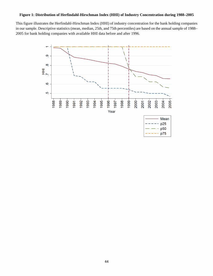
44
Figure 1: Distribution of Herfindahl-Hirschman Index (HHI) of Industry Concentration during 1988–2005
This figure illustrates the Herfindahl-Hirschman Index (HHI) of industry concentration for the bank holding companies in our sample. Descriptive statistics (mean, median, 25th, and 75th percentiles) are based on the annual sample of 1988–2005 for bank holding companies with available HHI data before and after 1996.
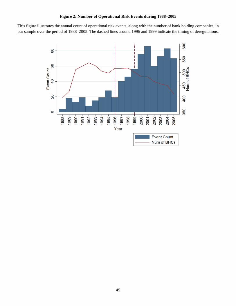
45
Figure 2: Number of Operational Risk Events during 1988–2005
This figure illustrates the annual count of operational risk events, along with the number of bank holding companies, in our sample over the period of 1988–2005. The dashed lines around 1996 and 1999 indicate the timing of deregulations.
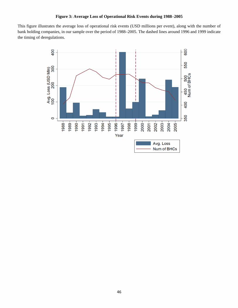
46
Figure 3: Average Loss of Operational Risk Events during 1988–2005
This figure illustrates the average loss of operational risk events (USD millions per event), along with the number of bank holding companies, in our sample over the period of 1988–2005. The dashed lines around 1996 and 1999 indicate the timing of deregulations.
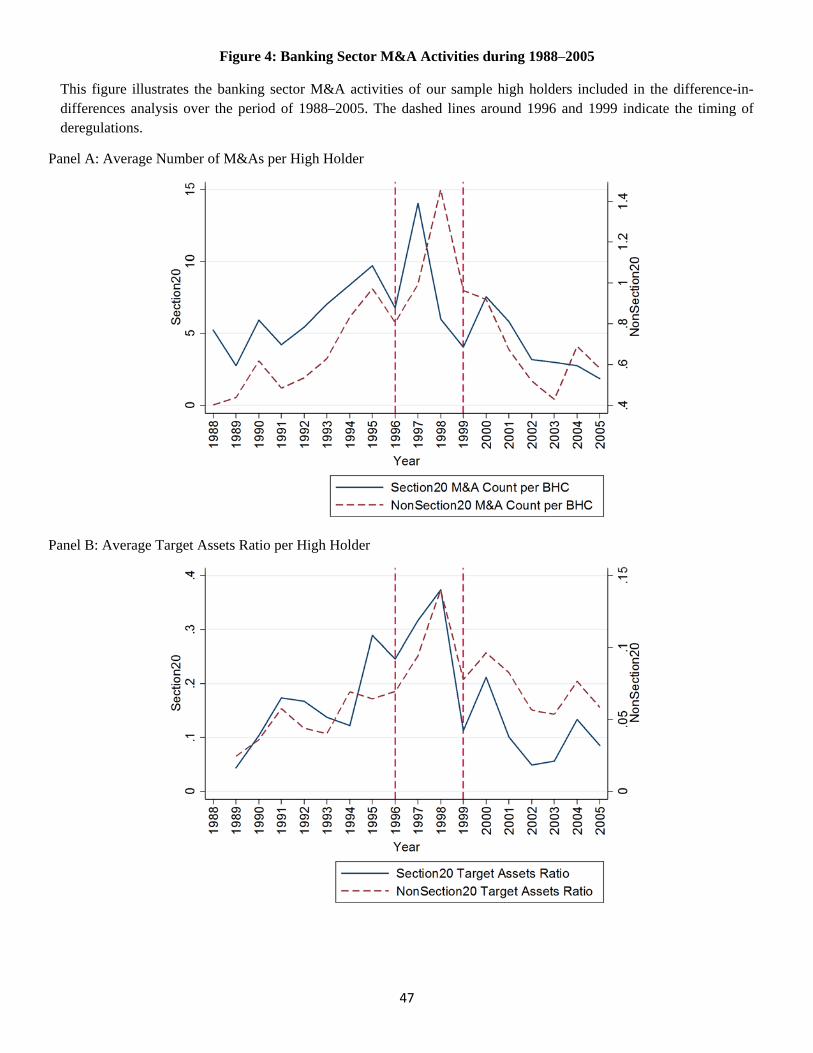
47
Figure 4: Banking Sector M&A Activities during 1988–2005
This figure illustrates the banking sector M&A activities of our sample high holders included in the difference-in-differences analysis over the period of 1988–2005. The dashed lines around 1996 and 1999 indicate the timing of deregulations.
Panel A: Average Number of M&As per High Holder
Panel B: Average Target Assets Ratio per High Holder
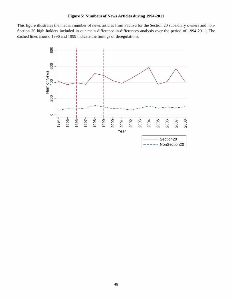
48
Figure 5: Numbers of News Articles during 1994-2011
This figure illustrates the median number of news articles from Factiva for the Section 20 subsidiary owners and non-Section 20 high holders included in our main difference-in-differences analysis over the period of 1994-2011. The dashed lines around 1996 and 1999 indicate the timings of deregulations.
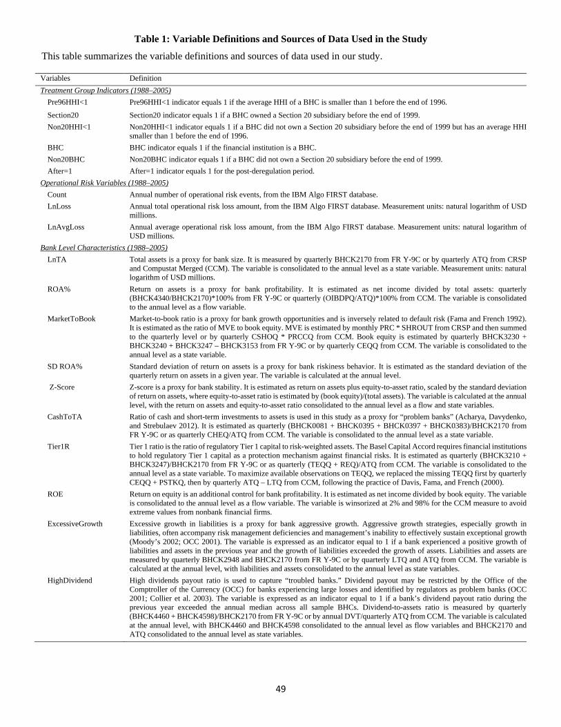
49
Table 1: Variable Definitions and Sources of Data Used in the Study
This table summarizes the variable definitions and sources of data used in our study. Variables Definition Treatment Group Indicators (1988–2005)
Pre96HHI<1 Pre96HHI<1 indicator equals 1 if the average HHI of a BHC is smaller than 1 before the end of 1996.
Section20 Section20 indicator equals 1 if a BHC owned a Section 20 subsidiary before the end of 1999. Non20HHI<1 Non20HHI<1 indicator equals 1 if a BHC did not own a Section 20 subsidiary before the end of 1999 but has an average HHI
smaller than 1 before the end of 1996. BHC BHC indicator equals 1 if the financial institution is a BHC. Non20BHC Non20BHC indicator equals 1 if a BHC did not own a Section 20 subsidiary before the end of 1999. After=1 After=1 indicator equals 1 for the post-deregulation period.
Operational Risk Variables (1988–2005) Count Annual number of operational risk events, from the IBM Algo FIRST database. LnLoss Annual total operational risk loss amount, from the IBM Algo FIRST database. Measurement units: natural logarithm of USD
millions. LnAvgLoss Annual average operational risk loss amount, from the IBM Algo FIRST database. Measurement units: natural logarithm of
USD millions. Bank Level Characteristics (1988–2005)
LnTA Total assets is a proxy for bank size. It is measured by quarterly BHCK2170 from FR Y-9C or by quarterly ATQ from CRSP and Compustat Merged (CCM). The variable is consolidated to the annual level as a state variable. Measurement units: natural logarithm of USD millions.
ROA% Return on assets is a proxy for bank profitability. It is estimated as net income divided by total assets: quarterly (BHCK4340/BHCK2170)*100% from FR Y-9C or quarterly (OIBDPQ/ATQ)*100% from CCM. The variable is consolidated to the annual level as a flow variable.
MarketToBook Market-to-book ratio is a proxy for bank growth opportunities and is inversely related to default risk (Fama and French 1992). It is estimated as the ratio of MVE to book equity. MVE is estimated by monthly PRC * SHROUT from CRSP and then summed to the quarterly level or by quarterly CSHOQ * PRCCQ from CCM. Book equity is estimated by quarterly BHCK3230 + BHCK3240 + BHCK3247 – BHCK3153 from FR Y-9C or by quarterly CEQQ from CCM. The variable is consolidated to the annual level as a state variable.
SD ROA% Standard deviation of return on assets is a proxy for bank riskiness behavior. It is estimated as the standard deviation of the quarterly return on assets in a given year. The variable is calculated at the annual level.
Z-Score Z-score is a proxy for bank stability. It is estimated as return on assets plus equity-to-asset ratio, scaled by the standard deviation of return on assets, where equity-to-asset ratio is estimated by (book equity)/(total assets). The variable is calculated at the annual level, with the return on assets and equity-to-asset ratio consolidated to the annual level as a flow and state variables.
CashToTA Ratio of cash and short-term investments to assets is used in this study as a proxy for “problem banks” (Acharya, Davydenko, and Strebulaev 2012). It is estimated as quarterly (BHCK0081 + BHCK0395 + BHCK0397 + BHCK0383)/BHCK2170 from FR Y-9C or as quarterly CHEQ/ATQ from CCM. The variable is consolidated to the annual level as a state variable.
Tier1R Tier 1 ratio is the ratio of regulatory Tier 1 capital to risk-weighted assets. The Basel Capital Accord requires financial institutions to hold regulatory Tier 1 capital as a protection mechanism against financial risks. It is estimated as quarterly (BHCK3210 + BHCK3247)/BHCK2170 from FR Y-9C or as quarterly (TEQQ + REQ)/ATQ from CCM. The variable is consolidated to the annual level as a state variable. To maximize available observations on TEQQ, we replaced the missing TEQQ first by quarterly CEQQ + PSTKQ, then by quarterly ATQ – LTQ from CCM, following the practice of Davis, Fama, and French (2000).
ROE Return on equity is an additional control for bank profitability. It is estimated as net income divided by book equity. The variable is consolidated to the annual level as a flow variable. The variable is winsorized at 2% and 98% for the CCM measure to avoid extreme values from nonbank financial firms.
ExcessiveGrowth Excessive growth in liabilities is a proxy for bank aggressive growth. Aggressive growth strategies, especially growth in liabilities, often accompany risk management deficiencies and management’s inability to effectively sustain exceptional growth (Moody’s 2002; OCC 2001). The variable is expressed as an indicator equal to 1 if a bank experienced a positive growth of liabilities and assets in the previous year and the growth of liabilities exceeded the growth of assets. Liabilities and assets are measured by quarterly BHCK2948 and BHCK2170 from FR Y-9C or by quarterly LTQ and ATQ from CCM. The variable is calculated at the annual level, with liabilities and assets consolidated to the annual level as state variables.
HighDividend High dividends payout ratio is used to capture “troubled banks.” Dividend payout may be restricted by the Office of the Comptroller of the Currency (OCC) for banks experiencing large losses and identified by regulators as problem banks (OCC 2001; Collier et al. 2003). The variable is expressed as an indicator equal to 1 if a bank’s dividend payout ratio during the previous year exceeded the annual median across all sample BHCs. Dividend-to-assets ratio is measured by quarterly (BHCK4460 + BHCK4598)/BHCK2170 from FR Y-9C or by annual DVT/quarterly ATQ from CCM. The variable is calculated at the annual level, with BHCK4460 and BHCK4598 consolidated to the annual level as flow variables and BHCK2170 and ATQ consolidated to the annual level as state variables.
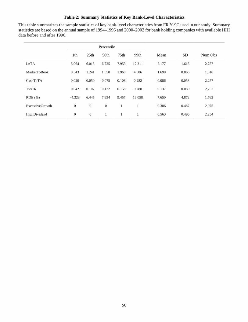
50
Table 2: Summary Statistics of Key Bank-Level Characteristics
This table summarizes the sample statistics of key bank-level characteristics from FR Y-9C used in our study. Summary statistics are based on the annual sample of 1994–1996 and 2000–2002 for bank holding companies with available HHI data before and after 1996.
Percentile
1th 25th 50th 75th 99th Mean SD Num Obs
LnTA 5.064 6.015 6.725 7.953 12.311 7.177 1.613 2,257 MarketToBook 0.543 1.241 1.558 1.960 4.686 1.699 0.866 1,816 CashToTA 0.020 0.050 0.075 0.108 0.282 0.086 0.053 2,257 Tier1R 0.042 0.107 0.132 0.158 0.288 0.137 0.059 2,257 ROE (%) -4.323 6.445 7.934 9.457 16.058 7.650 4.872 1,762 ExcessiveGrowth 0 0 0 1 1 0.386 0.487 2,075 HighDividend 0 0 1 1 1 0.563 0.496 2,254
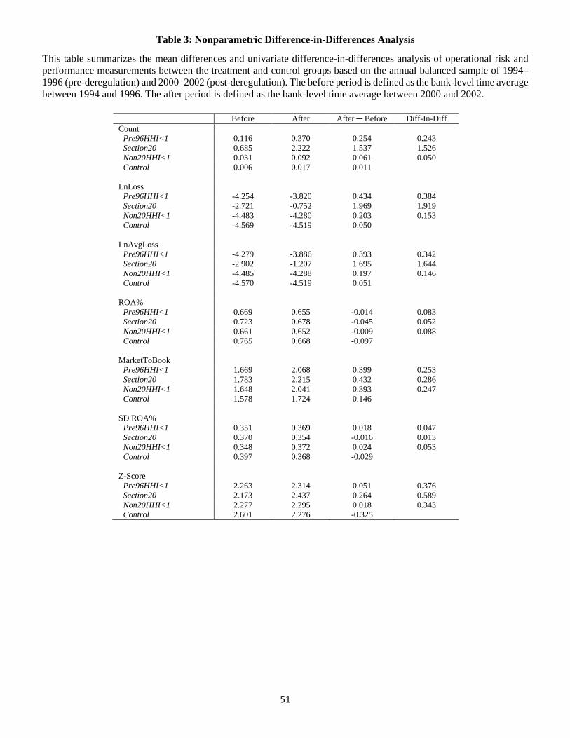
51
Table 3: Nonparametric Difference-in-Differences Analysis
This table summarizes the mean differences and univariate difference-in-differences analysis of operational risk and performance measurements between the treatment and control groups based on the annual balanced sample of 1994–1996 (pre-deregulation) and 2000–2002 (post-deregulation). The before period is defined as the bank-level time average between 1994 and 1996. The after period is defined as the bank-level time average between 2000 and 2002.
Before After After ─ Before Diff-In-Diff Count
Pre96HHI<1 0.116 0.370 0.254 0.243 Section20 0.685 2.222 1.537 1.526 Non20HHI<1 0.031 0.092 0.061 0.050 Control 0.006 0.017 0.011
LnLoss
Pre96HHI<1 -4.254 -3.820 0.434 0.384 Section20 -2.721 -0.752 1.969 1.919 Non20HHI<1 -4.483 -4.280 0.203 0.153 Control -4.569 -4.519 0.050
LnAvgLoss
Pre96HHI<1 -4.279 -3.886 0.393 0.342 Section20 -2.902 -1.207 1.695 1.644 Non20HHI<1 -4.485 -4.288 0.197 0.146 Control -4.570 -4.519 0.051
ROA%
Pre96HHI<1 0.669 0.655 -0.014 0.083 Section20 0.723 0.678 -0.045 0.052 Non20HHI<1 0.661 0.652 -0.009 0.088 Control 0.765 0.668 -0.097
MarketToBook
Pre96HHI<1 1.669 2.068 0.399 0.253 Section20 1.783 2.215 0.432 0.286 Non20HHI<1 1.648 2.041 0.393 0.247 Control 1.578 1.724 0.146
SD ROA%
Pre96HHI<1 0.351 0.369 0.018 0.047 Section20 0.370 0.354 -0.016 0.013 Non20HHI<1 0.348 0.372 0.024 0.053 Control 0.397 0.368 -0.029
Z-Score
Pre96HHI<1 2.263 2.314 0.051 0.376 Section20 2.173 2.437 0.264 0.589 Non20HHI<1 2.277 2.295 0.018 0.343 Control 2.601 2.276 -0.325
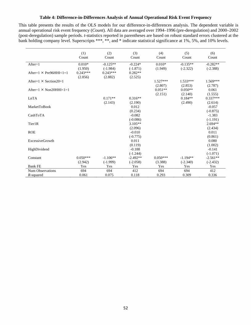
52
Table 4: Difference-in-Differences Analysis of Annual Operational Risk Event Frequency
This table presents the results of the OLS models for our difference-in-differences analysis. The dependent variable is annual operational risk event frequency (Count). All data are averaged over 1994–1996 (pre-deregulation) and 2000–2002 (post-deregulation) sample periods. t-statistics reported in parentheses are based on robust standard errors clustered at the bank holding company level. Superscripts ***, **, and * indicate statistical significance at 1%, 5%, and 10% levels.
(1) (2) (3) (4) (5) (6) Count Count Count Count Count Count
After=1 0.010* -0.125** -0.224* 0.010* -0.135** -0.282** (1.950) (-1.984) (-1.871) (1.949) (-2.322) (-2.388) After=1 Pre96HHI<1=1 0.243*** 0.243*** 0.282** (2.856) (2.882) (2.525) After=1 Section20=1 1.527*** 1.533*** 1.569*** (2.807) (2.853) (2.787) After=1 Non20HHI<1=1 0.051** 0.050** 0.061 (2.151) (2.140) (1.555) LnTA 0.171** 0.316** 0.184** 0.337*** (2.143) (2.190) (2.490) (2.614) MarketToBook 0.012 -0.057 (0.234) (-0.875) CashToTA -0.082 -1.383 (-0.086) (-1.191) Tier1R 3.105** 2.694** (2.096) (2.434) ROE -0.010 0.011 (-0.775) (0.861) ExcessiveGrowth 0.011 0.080 (0.119) (1.002) HighDividend -0.188 -0.141 (-1.244) (-1.071) Constant 0.050*** -1.106** -2.492** 0.050*** -1.194** -2.561** (2.942) (-1.999) (-2.058) (3.388) (-2.340) (-2.432) Bank FE Yes Yes Yes Yes Yes Yes Num Observations 694 694 412 694 694 412 R-squared 0.061 0.075 0.118 0.293 0.309 0.336
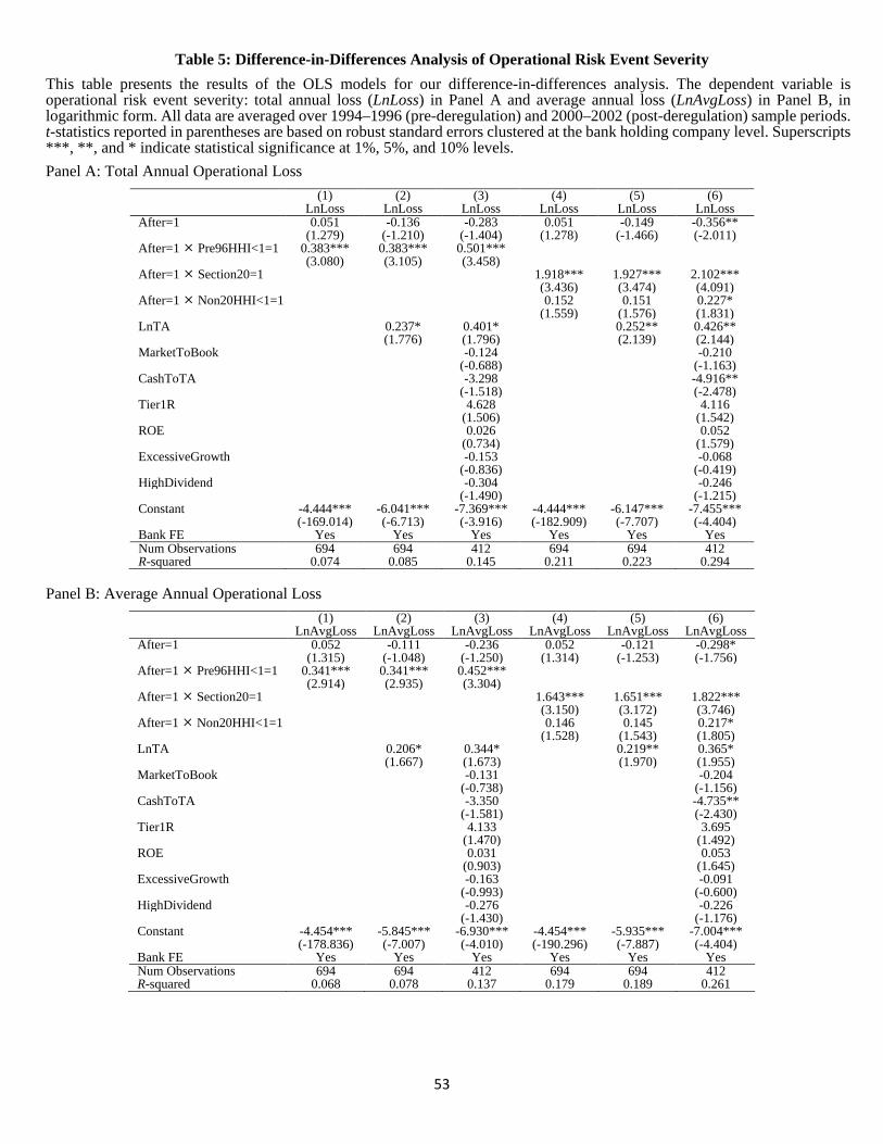
53
Table 5: Difference-in-Differences Analysis of Operational Risk Event Severity This table presents the results of the OLS models for our difference-in-differences analysis. The dependent variable is operational risk event severity: total annual loss (LnLoss) in Panel A and average annual loss (LnAvgLoss) in Panel B, in logarithmic form. All data are averaged over 1994–1996 (pre-deregulation) and 2000–2002 (post-deregulation) sample periods. t-statistics reported in parentheses are based on robust standard errors clustered at the bank holding company level. Superscripts ***, **, and * indicate statistical significance at 1%, 5%, and 10% levels. Panel A: Total Annual Operational Loss
(1) (2) (3) (4) (5) (6) LnLoss LnLoss LnLoss LnLoss LnLoss LnLoss After=1 0.051 -0.136 -0.283 0.051 -0.149 -0.356** (1.279) (-1.210) (-1.404) (1.278) (-1.466) (-2.011) After=1 Pre96HHI<1=1 0.383*** 0.383*** 0.501*** (3.080) (3.105) (3.458) After=1 Section20=1 1.918*** 1.927*** 2.102*** (3.436) (3.474) (4.091) After=1 Non20HHI<1=1 0.152 0.151 0.227* (1.559) (1.576) (1.831) LnTA 0.237* 0.401* 0.252** 0.426** (1.776) (1.796) (2.139) (2.144) MarketToBook -0.124 -0.210 (-0.688) (-1.163) CashToTA -3.298 -4.916** (-1.518) (-2.478) Tier1R 4.628 4.116 (1.506) (1.542) ROE 0.026 0.052 (0.734) (1.579) ExcessiveGrowth -0.153 -0.068 (-0.836) (-0.419) HighDividend -0.304 -0.246 (-1.490) (-1.215) Constant -4.444*** -6.041*** -7.369*** -4.444*** -6.147*** -7.455*** (-169.014) (-6.713) (-3.916) (-182.909) (-7.707) (-4.404) Bank FE Yes Yes Yes Yes Yes Yes Num Observations 694 694 412 694 694 412 R-squared 0.074 0.085 0.145 0.211 0.223 0.294
Panel B: Average Annual Operational Loss
(1) (2) (3) (4) (5) (6) LnAvgLoss LnAvgLoss LnAvgLoss LnAvgLoss LnAvgLoss LnAvgLoss After=1 0.052 -0.111 -0.236 0.052 -0.121 -0.298* (1.315) (-1.048) (-1.250) (1.314) (-1.253) (-1.756) After=1 Pre96HHI<1=1 0.341*** 0.341*** 0.452*** (2.914) (2.935) (3.304) After=1 Section20=1 1.643*** 1.651*** 1.822*** (3.150) (3.172) (3.746) After=1 Non20HHI<1=1 0.146 0.145 0.217* (1.528) (1.543) (1.805) LnTA 0.206* 0.344* 0.219** 0.365* (1.667) (1.673) (1.970) (1.955) MarketToBook -0.131 -0.204 (-0.738) (-1.156) CashToTA -3.350 -4.735** (-1.581) (-2.430) Tier1R 4.133 3.695 (1.470) (1.492) ROE 0.031 0.053 (0.903) (1.645) ExcessiveGrowth -0.163 -0.091 (-0.993) (-0.600) HighDividend -0.276 -0.226 (-1.430) (-1.176) Constant -4.454*** -5.845*** -6.930*** -4.454*** -5.935*** -7.004*** (-178.836) (-7.007) (-4.010) (-190.296) (-7.887) (-4.404) Bank FE Yes Yes Yes Yes Yes Yes Num Observations 694 694 412 694 694 412 R-squared 0.068 0.078 0.137 0.179 0.189 0.261
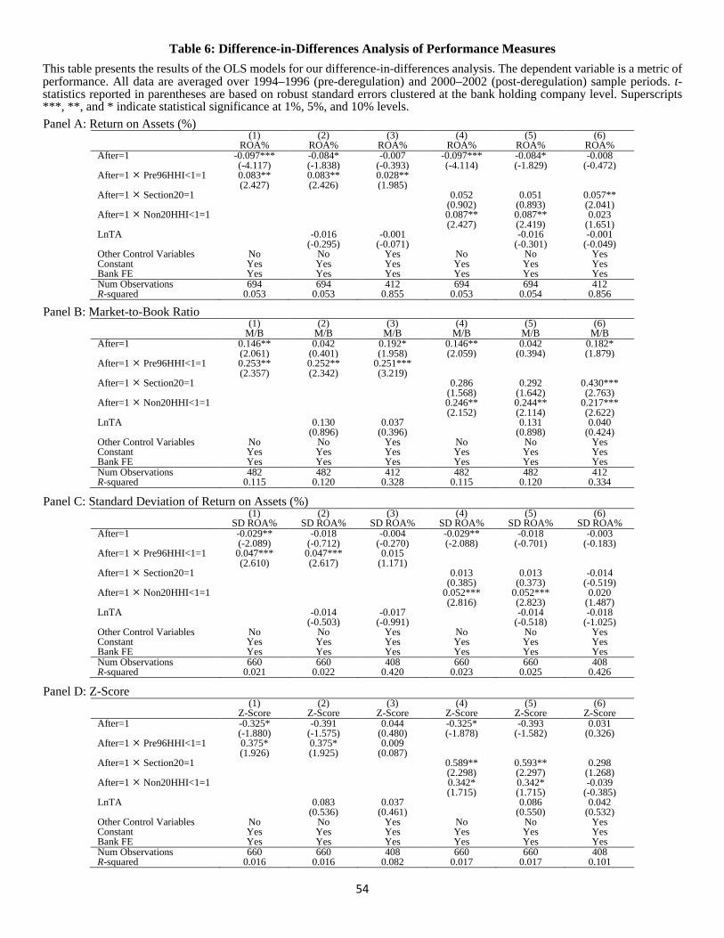
54
Table 6: Difference-in-Differences Analysis of Performance Measures This table presents the results of the OLS models for our difference-in-differences analysis. The dependent variable is a metric of performance. All data are averaged over 1994–1996 (pre-deregulation) and 2000–2002 (post-deregulation) sample periods. t-statistics reported in parentheses are based on robust standard errors clustered at the bank holding company level. Superscripts ***, **, and * indicate statistical significance at 1%, 5%, and 10% levels. Panel A: Return on Assets (%)
(1) (2) (3) (4) (5) (6) ROA% ROA% ROA% ROA% ROA% ROA% After=1 -0.097*** -0.084* -0.007 -0.097*** -0.084* -0.008 (-4.117) (-1.838) (-0.393) (-4.114) (-1.829) (-0.472) After=1 Pre96HHI<1=1 0.083** 0.083** 0.028** (2.427) (2.426) (1.985) After=1 Section20=1 0.052 0.051 0.057** (0.902) (0.893) (2.041) After=1 Non20HHI<1=1 0.087** 0.087** 0.023 (2.427) (2.419) (1.651) LnTA -0.016 -0.001 -0.016 -0.001 (-0.295) (-0.071) (-0.301) (-0.049) Other Control Variables No No Yes No No Yes Constant Yes Yes Yes Yes Yes Yes Bank FE Yes Yes Yes Yes Yes Yes Num Observations 694 694 412 694 694 412 R-squared 0.053 0.053 0.855 0.053 0.054 0.856
Panel B: Market-to-Book Ratio (1) (2) (3) (4) (5) (6) M/B M/B M/B M/B M/B M/B After=1 0.146** 0.042 0.192* 0.146** 0.042 0.182* (2.061) (0.401) (1.958) (2.059) (0.394) (1.879) After=1 Pre96HHI<1=1 0.253** 0.252** 0.251*** (2.357) (2.342) (3.219) After=1 Section20=1 0.286 0.292 0.430*** (1.568) (1.642) (2.763) After=1 Non20HHI<1=1 0.246** 0.244** 0.217*** (2.152) (2.114) (2.622) LnTA 0.130 0.037 0.131 0.040 (0.896) (0.396) (0.898) (0.424) Other Control Variables No No Yes No No Yes Constant Yes Yes Yes Yes Yes Yes Bank FE Yes Yes Yes Yes Yes Yes Num Observations 482 482 412 482 482 412 R-squared 0.115 0.120 0.328 0.115 0.120 0.334
Panel C: Standard Deviation of Return on Assets (%) (1) (2) (3) (4) (5) (6) SD ROA% SD ROA% SD ROA% SD ROA% SD ROA% SD ROA% After=1 -0.029** -0.018 -0.004 -0.029** -0.018 -0.003 (-2.089) (-0.712) (-0.270) (-2.088) (-0.701) (-0.183) After=1 Pre96HHI<1=1 0.047*** 0.047*** 0.015 (2.610) (2.617) (1.171) After=1 Section20=1 0.013 0.013 -0.014 (0.385) (0.373) (-0.519) After=1 Non20HHI<1=1 0.052*** 0.052*** 0.020 (2.816) (2.823) (1.487) LnTA -0.014 -0.017 -0.014 -0.018 (-0.503) (-0.991) (-0.518) (-1.025) Other Control Variables No No Yes No No Yes Constant Yes Yes Yes Yes Yes Yes Bank FE Yes Yes Yes Yes Yes Yes Num Observations 660 660 408 660 660 408 R-squared 0.021 0.022 0.420 0.023 0.025 0.426
Panel D: Z-Score (1) (2) (3) (4) (5) (6) Z-Score Z-Score Z-Score Z-Score Z-Score Z-Score After=1 -0.325* -0.391 0.044 -0.325* -0.393 0.031 (-1.880) (-1.575) (0.480) (-1.878) (-1.582) (0.326) After=1 Pre96HHI<1=1 0.375* 0.375* 0.009 (1.926) (1.925) (0.087) After=1 Section20=1 0.589** 0.593** 0.298 (2.298) (2.297) (1.268) After=1 Non20HHI<1=1 0.342* 0.342* -0.039 (1.715) (1.715) (-0.385) LnTA 0.083 0.037 0.086 0.042 (0.536) (0.461) (0.550) (0.532) Other Control Variables No No Yes No No Yes Constant Yes Yes Yes Yes Yes Yes Bank FE Yes Yes Yes Yes Yes Yes Num Observations 660 660 408 660 660 408 R-squared 0.016 0.016 0.082 0.017 0.017 0.101
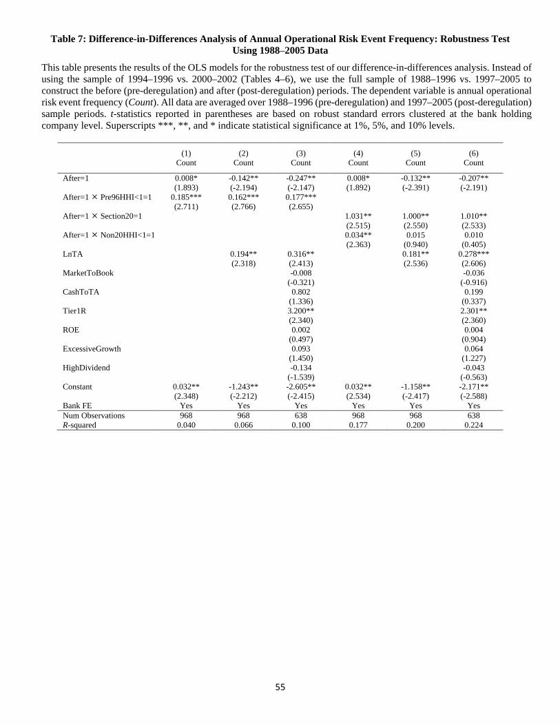
55
Table 7: Difference-in-Differences Analysis of Annual Operational Risk Event Frequency: Robustness Test Using 1988–2005 Data
This table presents the results of the OLS models for the robustness test of our difference-in-differences analysis. Instead of using the sample of 1994–1996 vs. 2000–2002 (Tables 4–6), we use the full sample of 1988–1996 vs. 1997–2005 to construct the before (pre-deregulation) and after (post-deregulation) periods. The dependent variable is annual operational risk event frequency (Count). All data are averaged over 1988–1996 (pre-deregulation) and 1997–2005 (post-deregulation) sample periods. t-statistics reported in parentheses are based on robust standard errors clustered at the bank holding company level. Superscripts ***, **, and * indicate statistical significance at 1%, 5%, and 10% levels.
(1) (2) (3) (4) (5) (6) Count Count Count Count Count Count
After=1 0.008* -0.142** -0.247** 0.008* -0.132** -0.207** (1.893) (-2.194) (-2.147) (1.892) (-2.391) (-2.191) After=1 Pre96HHI<1=1 0.185*** 0.162*** 0.177*** (2.711) (2.766) (2.655) After=1 Section20=1 1.031** 1.000** 1.010** (2.515) (2.550) (2.533) After=1 Non20HHI<1=1 0.034** 0.015 0.010 (2.363) (0.940) (0.405) LnTA 0.194** 0.316** 0.181** 0.278*** (2.318) (2.413) (2.536) (2.606) MarketToBook -0.008 -0.036 (-0.321) (-0.916) CashToTA 0.802 0.199 (1.336) (0.337) Tier1R 3.200** 2.301** (2.340) (2.360) ROE 0.002 0.004 (0.497) (0.904) ExcessiveGrowth 0.093 0.064 (1.450) (1.227) HighDividend -0.134 -0.043 (-1.539) (-0.563) Constant 0.032** -1.243** -2.605** 0.032** -1.158** -2.171** (2.348) (-2.212) (-2.415) (2.534) (-2.417) (-2.588) Bank FE Yes Yes Yes Yes Yes Yes Num Observations 968 968 638 968 968 638 R-squared 0.040 0.066 0.100 0.177 0.200 0.224
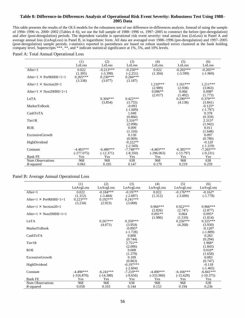
56
Table 8: Difference-in-Differences Analysis of Operational Risk Event Severity: Robustness Test Using 1988–2005 Data
This table presents the results of the OLS models for the robustness test of our difference-in-differences analysis. Instead of using the sample of 1994–1996 vs. 2000–2002 (Tables 4–6), we use the full sample of 1988–1996 vs. 1997–2005 to construct the before (pre-deregulation) and after (post-deregulation) periods. The dependent variable is operational risk event severity: total annual loss (LnLoss) in Panel A and average annual loss (LnAvgLoss) in Panel B, in logarithmic form. All data are averaged over 1988–1996 (pre-deregulation) and 1997–2005 (post-deregulation) sample periods. t-statistics reported in parentheses are based on robust standard errors clustered at the bank holding company level. Superscripts ***, **, and * indicate statistical significance at 1%, 5%, and 10% levels.
Panel A: Total Annual Operational Loss
(1) (2) (3) (4) (5) (6) LnLoss LnLoss LnLoss LnLoss LnLoss LnLoss After=1 0.022 -0.213*** -0.250** 0.022 -0.202*** -0.205** (1.305) (-3.398) (-2.251) (1.304) (-3.599) (-1.969) After=1 Pre96HHI<1=1 0.265*** 0.230*** 0.284*** (3.338) (3.077) (3.187) After=1 Section20=1 1.210*** 1.161*** 1.211*** (2.989) (2.938) (3.063) After=1 Non20HHI<1=1 0.096** 0.066 0.098* (2.017) (1.492) (1.773) LnTA 0.304*** 0.422*** 0.290*** 0.379*** (3.854) (3.755) (4.138) (3.841) MarketToBook -0.093 -0.125* (-1.609) (-1.797) CashToTA 1.049 0.378 (0.866) (0.359) Tier1R 3.316** 2.315* (2.098) (1.942) ROE 0.009 0.011 (1.316) (1.648) ExcessiveGrowth 0.130 0.097 (0.909) (0.780) HighDividend -0.222** -0.120 (-2.569) (-1.319) Constant -4.483*** -6.480*** -7.748*** -4.483*** -6.385*** -7.265*** (-277.075) (-12.371) (-8.350) (-296.063) (-13.797) (-9.231) Bank FE Yes Yes Yes Yes Yes Yes Num Observations 968 968 638 968 968 638 R-squared 0.061 0.105 0.147 0.179 0.219 0.259
Panel B: Average Annual Operational Loss
(1) (2) (3) (4) (5) (6) LnAvgLoss LnAvgLoss LnAvgLoss LnAvgLoss LnAvgLoss LnAvgLoss After=1 0.022 -0.184*** -0.197** 0.022 -0.176*** -0.162* (1.312) (-3.484) (-2.087) (1.312) (-3.600) (-1.778) After=1 Pre96HHI<1=1 0.223*** 0.192*** 0.241*** (3.234) (2.923) (3.068) After=1 Section20=1 0.966*** 0.922*** 0.966*** (2.826) (2.747) (2.877) After=1 Non20HHI<1=1 0.091** 0.064 0.095* (1.986) (1.510) (1.814) LnTA 0.267*** 0.359*** 0.256*** 0.325*** (4.071) (3.954) (4.268) (3.930) MarketToBook -0.095* -0.120* (-1.728) (-1.889) CashToTA 0.808 0.283 (0.744) (0.294) Tier1R 2.751** 1.968* (2.006) (1.843) ROE 0.008 0.010* (1.379) (1.658) ExcessiveGrowth 0.109 0.083 (0.863) (0.747) HighDividend -0.197*** -0.118 (-2.604) (-1.465) Constant -4.490*** -6.241*** -7.219*** -4.490*** -6.166*** -6.841*** (-316.870) (-14.388) (-9.656) (-333.960) (-15.629) (-10.375) Bank FE Yes Yes Yes Yes Yes Yes Num Observations 968 968 638 968 968 638 R-squared 0.058 0.103 0.144 0.153 0.194 0.236
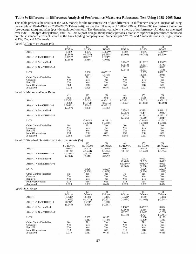
57
Table 9: Difference-in-Differences Analysis of Performance Measures: Robustness Test Using 1988–2005 Data
This table presents the results of the OLS models for the robustness test of our difference-in-differences analysis. Instead of using the sample of 1994–1996 vs. 2000–2002 (Tables 4–6), we use the full sample of 1988–1996 vs. 1997–2005 to construct the before (pre-deregulation) and after (post-deregulation) periods. The dependent variable is a metric of performance. All data are averaged over 1988–1996 (pre-deregulation) and 1997–2005 (post-deregulation) sample periods. t-statistics reported in parentheses are based on robust standard errors clustered at the bank holding company level. Superscripts ***, **, and * indicate statistical significance at 1%, 5%, and 10% levels. Panel A: Return on Assets (%)
(1) (2) (3) (4) (5) (6) ROA% ROA% ROA% ROA% ROA% ROA% After=1 0.002 -0.026 -0.064*** 0.002 -0.025 -0.062*** (0.108) (-0.757) (-3.285) (0.108) (-0.742) (-3.210) After=1 Pre96HHI<1=1 0.069** 0.065** 0.024** (2.554) (2.380) (2.033) After=1 Section20=1 0.114** 0.108** 0.051** (2.312) (2.197) (2.349) After=1 Non20HHI<1=1 0.061** 0.058** 0.019 (2.145) (2.001) (1.531) LnTA 0.036 0.039*** 0.035 0.038*** (1.184) (3.168) (1.165) (3.026) Other Control Variables No No Yes No No Yes Constant Yes Yes Yes Yes Yes Yes Bank FE Yes Yes Yes Yes Yes Yes Num Observations 968 968 638 968 968 638 R-squared 0.022 0.025 0.877 0.023 0.027 0.878
Panel B: Market-to-Book Ratio (1) (2) (3) (4) (5) (6) M/B M/B M/B M/B M/B M/B After=1 0.737*** 0.845*** 0.904*** 0.737*** 0.847*** 0.906*** (13.986) (11.751) (11.015) (13.977) (11.811) (11.093) After=1 Pre96HHI<1=1 0.208*** 0.229*** 0.312*** (2.797) (2.990) (4.497) After=1 Section20=1 0.359** 0.388** 0.446*** (2.257) (2.457) (2.932) After=1 Non20HHI<1=1 0.177** 0.196** 0.283*** (2.326) (2.519) (4.045) LnTA -0.145** -0.149** -0.148** -0.154** (-2.129) (-2.280) (-2.182) (-2.368) Other Control Variables No No Yes No No Yes Constant Yes Yes Yes Yes Yes Yes Bank FE Yes Yes Yes Yes Yes Yes Num Observations 730 730 638 730 730 638 R-squared 0.584 0.589 0.674 0.586 0.591 0.676
Panel C: Standard Deviation of Return on Assets (%) (1) (2) (3) (4) (5) (6) SD ROA% SD ROA% SD ROA% SD ROA% SD ROA% SD ROA% After=1 -0.002 -0.022 -0.066*** -0.002 -0.022 -0.066*** (-0.184) (-1.244) (-3.574) (-0.184) (-1.243) (-3.554) After=1 Pre96HHI<1=1 0.035*** 0.032*** 0.006 (2.864) (2.610) (0.529) After=1 Section20=1 0.035 0.031 0.010 (1.400) (1.233) (0.403) After=1 Non20HHI<1=1 0.034*** 0.032** 0.006 (2.808) (2.580) (0.467) LnTA 0.026 0.023* 0.026 0.023* (1.586) (1.871) (1.584) (1.832) Other Control Variables No No Yes No No Yes Constant Yes Yes Yes Yes Yes Yes Bank FE Yes Yes Yes Yes Yes Yes Num Observations 918 918 616 918 918 616 R-squared 0.023 0.032 0.404 0.023 0.032 0.404
Panel D: Z-Score (1) (2) (3) (4) (5) (6) Z-Score Z-Score Z-Score Z-Score Z-Score Z-Score After=1 -0.228* -0.309 -0.105 -0.228* -0.307 -0.103 (-1.675) (-1.471) (-0.971) (-1.674) (-1.463) (-0.944) After=1 Pre96HHI<1=1 0.284* 0.273* -0.018 (1.945) (1.959) (-0.267) After=1 Section20=1 0.438** 0.423** 0.054 (2.568) (2.568) (0.421) After=1 Non20HHI<1=1 0.255* 0.245* -0.033 (1.719) (1.724) (-0.481) LnTA 0.102 0.103 0.100 0.100 (0.813) (1.434) (0.800) (1.380) Other Control Variables No No Yes No No Yes Constant Yes Yes Yes Yes Yes Yes Bank FE Yes Yes Yes Yes Yes Yes Num Observations 918 918 616 918 918 616 R-squared 0.010 0.011 0.437 0.010 0.011 0.438
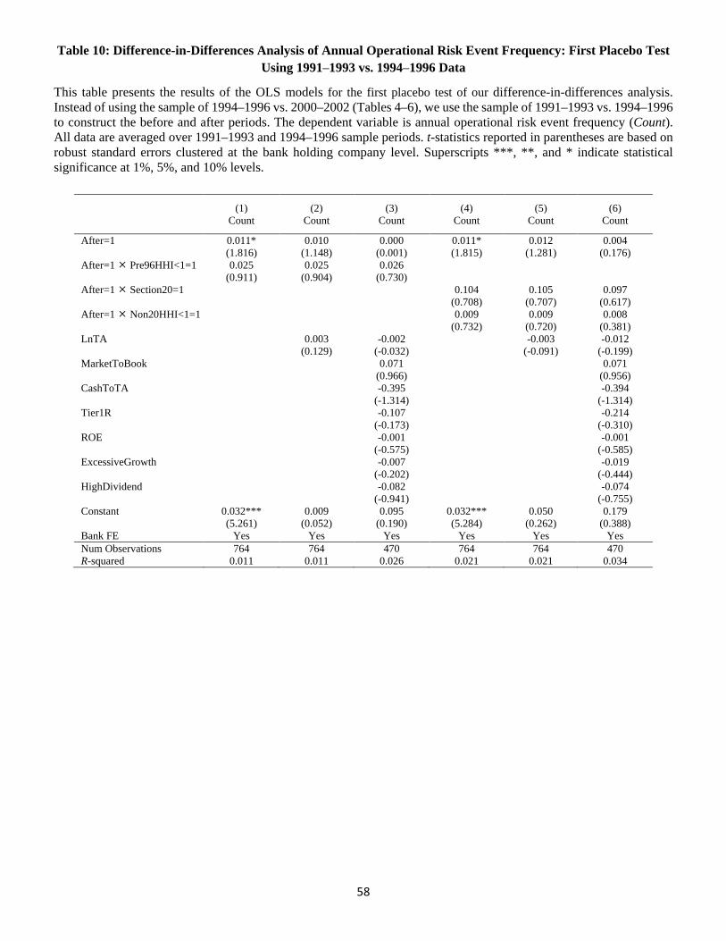
58
Table 10: Difference-in-Differences Analysis of Annual Operational Risk Event Frequency: First Placebo Test Using 1991–1993 vs. 1994–1996 Data
This table presents the results of the OLS models for the first placebo test of our difference-in-differences analysis. Instead of using the sample of 1994–1996 vs. 2000–2002 (Tables 4–6), we use the sample of 1991–1993 vs. 1994–1996 to construct the before and after periods. The dependent variable is annual operational risk event frequency (Count). All data are averaged over 1991–1993 and 1994–1996 sample periods. t-statistics reported in parentheses are based on robust standard errors clustered at the bank holding company level. Superscripts ***, **, and * indicate statistical significance at 1%, 5%, and 10% levels.
(1) (2) (3) (4) (5) (6) Count Count Count Count Count Count
After=1 0.011* 0.010 0.000 0.011* 0.012 0.004 (1.816) (1.148) (0.001) (1.815) (1.281) (0.176) After=1 Pre96HHI<1=1 0.025 0.025 0.026 (0.911) (0.904) (0.730) After=1 Section20=1 0.104 0.105 0.097 (0.708) (0.707) (0.617) After=1 Non20HHI<1=1 0.009 0.009 0.008 (0.732) (0.720) (0.381) LnTA 0.003 -0.002 -0.003 -0.012 (0.129) (-0.032) (-0.091) (-0.199) MarketToBook 0.071 0.071 (0.966) (0.956) CashToTA -0.395 -0.394 (-1.314) (-1.314) Tier1R -0.107 -0.214 (-0.173) (-0.310) ROE -0.001 -0.001 (-0.575) (-0.585) ExcessiveGrowth -0.007 -0.019 (-0.202) (-0.444) HighDividend -0.082 -0.074 (-0.941) (-0.755) Constant 0.032*** 0.009 0.095 0.032*** 0.050 0.179 (5.261) (0.052) (0.190) (5.284) (0.262) (0.388) Bank FE Yes Yes Yes Yes Yes Yes Num Observations 764 764 470 764 764 470 R-squared 0.011 0.011 0.026 0.021 0.021 0.034
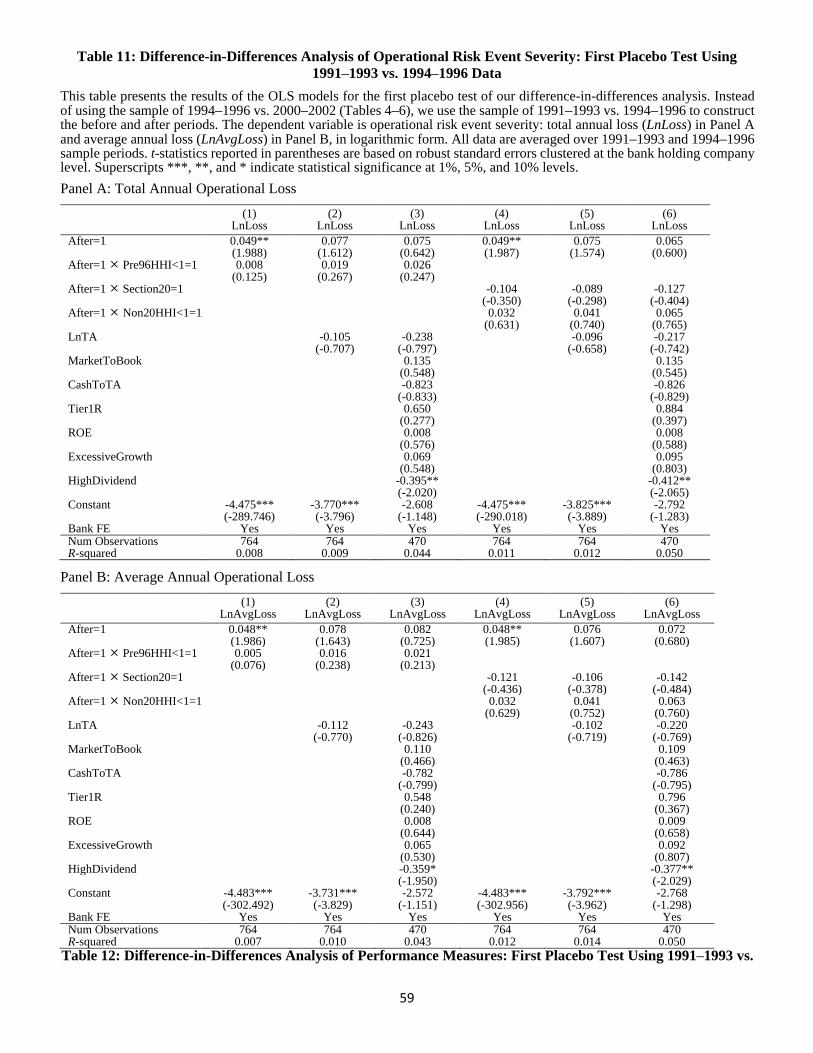
59
Table 11: Difference-in-Differences Analysis of Operational Risk Event Severity: First Placebo Test Using 1991–1993 vs. 1994–1996 Data
This table presents the results of the OLS models for the first placebo test of our difference-in-differences analysis. Instead of using the sample of 1994–1996 vs. 2000–2002 (Tables 4–6), we use the sample of 1991–1993 vs. 1994–1996 to construct the before and after periods. The dependent variable is operational risk event severity: total annual loss (LnLoss) in Panel A and average annual loss (LnAvgLoss) in Panel B, in logarithmic form. All data are averaged over 1991–1993 and 1994–1996 sample periods. t-statistics reported in parentheses are based on robust standard errors clustered at the bank holding company level. Superscripts ***, **, and * indicate statistical significance at 1%, 5%, and 10% levels. Panel A: Total Annual Operational Loss
(1) (2) (3) (4) (5) (6) LnLoss LnLoss LnLoss LnLoss LnLoss LnLoss After=1 0.049** 0.077 0.075 0.049** 0.075 0.065 (1.988) (1.612) (0.642) (1.987) (1.574) (0.600) After=1 Pre96HHI<1=1 0.008 0.019 0.026 (0.125) (0.267) (0.247) After=1 Section20=1 -0.104 -0.089 -0.127 (-0.350) (-0.298) (-0.404) After=1 Non20HHI<1=1 0.032 0.041 0.065 (0.631) (0.740) (0.765) LnTA -0.105 -0.238 -0.096 -0.217 (-0.707) (-0.797) (-0.658) (-0.742) MarketToBook 0.135 0.135 (0.548) (0.545) CashToTA -0.823 -0.826 (-0.833) (-0.829) Tier1R 0.650 0.884 (0.277) (0.397) ROE 0.008 0.008 (0.576) (0.588) ExcessiveGrowth 0.069 0.095 (0.548) (0.803) HighDividend -0.395** -0.412** (-2.020) (-2.065) Constant -4.475*** -3.770*** -2.608 -4.475*** -3.825*** -2.792 (-289.746) (-3.796) (-1.148) (-290.018) (-3.889) (-1.283) Bank FE Yes Yes Yes Yes Yes Yes Num Observations 764 764 470 764 764 470 R-squared 0.008 0.009 0.044 0.011 0.012 0.050
Panel B: Average Annual Operational Loss
(1) (2) (3) (4) (5) (6) LnAvgLoss LnAvgLoss LnAvgLoss LnAvgLoss LnAvgLoss LnAvgLoss After=1 0.048** 0.078 0.082 0.048** 0.076 0.072 (1.986) (1.643) (0.725) (1.985) (1.607) (0.680) After=1 Pre96HHI<1=1 0.005 0.016 0.021 (0.076) (0.238) (0.213) After=1 Section20=1 -0.121 -0.106 -0.142 (-0.436) (-0.378) (-0.484) After=1 Non20HHI<1=1 0.032 0.041 0.063 (0.629) (0.752) (0.760) LnTA -0.112 -0.243 -0.102 -0.220 (-0.770) (-0.826) (-0.719) (-0.769) MarketToBook 0.110 0.109 (0.466) (0.463) CashToTA -0.782 -0.786 (-0.799) (-0.795) Tier1R 0.548 0.796 (0.240) (0.367) ROE 0.008 0.009 (0.644) (0.658) ExcessiveGrowth 0.065 0.092 (0.530) (0.807) HighDividend -0.359* -0.377** (-1.950) (-2.029) Constant -4.483*** -3.731*** -2.572 -4.483*** -3.792*** -2.768 (-302.492) (-3.829) (-1.151) (-302.956) (-3.962) (-1.298) Bank FE Yes Yes Yes Yes Yes Yes Num Observations 764 764 470 764 764 470 R-squared 0.007 0.010 0.043 0.012 0.014 0.050
Table 12: Difference-in-Differences Analysis of Performance Measures: First Placebo Test Using 1991–1993 vs.
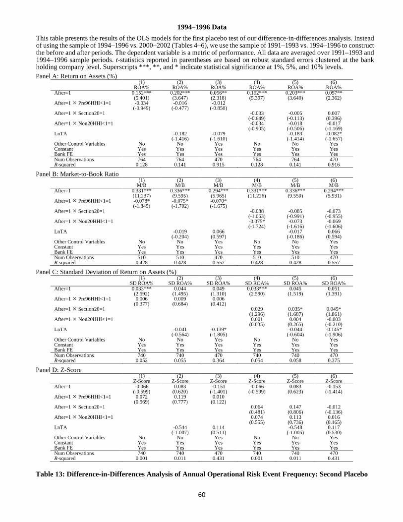
60
1994–1996 Data This table presents the results of the OLS models for the first placebo test of our difference-in-differences analysis. Instead of using the sample of 1994–1996 vs. 2000–2002 (Tables 4–6), we use the sample of 1991–1993 vs. 1994–1996 to construct the before and after periods. The dependent variable is a metric of performance. All data are averaged over 1991–1993 and 1994–1996 sample periods. t-statistics reported in parentheses are based on robust standard errors clustered at the bank holding company level. Superscripts ***, **, and * indicate statistical significance at 1%, 5%, and 10% levels. Panel A: Return on Assets (%)
(1) (2) (3) (4) (5) (6) ROA% ROA% ROA% ROA% ROA% ROA% After=1 0.152*** 0.202*** 0.056** 0.152*** 0.203*** 0.057** (5.401) (3.647) (2.318) (5.397) (3.640) (2.362) After=1 Pre96HHI<1=1 -0.034 -0.016 -0.012 (-0.949) (-0.477) (-0.850) After=1 Section20=1 -0.033 -0.005 0.007 (-0.649) (-0.113) (0.396) After=1 Non20HHI<1=1 -0.034 -0.018 -0.017 (-0.905) (-0.506) (-1.169) LnTA -0.182 -0.079 -0.183 -0.082* (-1.416) (-1.610) (-1.414) (-1.657) Other Control Variables No No Yes No No Yes Constant Yes Yes Yes Yes Yes Yes Bank FE Yes Yes Yes Yes Yes Yes Num Observations 764 764 470 764 764 470 R-squared 0.128 0.141 0.915 0.128 0.141 0.916
Panel B: Market-to-Book Ratio (1) (2) (3) (4) (5) (6) M/B M/B M/B M/B M/B M/B After=1 0.331*** 0.336*** 0.294*** 0.331*** 0.336*** 0.294*** (11.237) (9.595) (5.965) (11.226) (9.550) (5.931) After=1 Pre96HHI<1=1 -0.078* -0.075* -0.070* (-1.849) (-1.702) (-1.675) After=1 Section20=1 -0.088 -0.085 -0.073 (-1.063) (-0.991) (-0.955) After=1 Non20HHI<1=1 -0.075* -0.073 -0.069 (-1.724) (-1.616) (-1.606) LnTA -0.019 0.066 -0.017 0.066 (-0.204) (0.597) (-0.186) (0.594) Other Control Variables No No Yes No No Yes Constant Yes Yes Yes Yes Yes Yes Bank FE Yes Yes Yes Yes Yes Yes Num Observations 510 510 470 510 510 470 R-squared 0.428 0.428 0.557 0.428 0.428 0.557
Panel C: Standard Deviation of Return on Assets (%) (1) (2) (3) (4) (5) (6) SD ROA% SD ROA% SD ROA% SD ROA% SD ROA% SD ROA% After=1 0.033*** 0.044 0.049 0.033*** 0.045 0.051 (2.592) (1.495) (1.310) (2.590) (1.519) (1.391) After=1 Pre96HHI<1=1 0.006 0.009 0.006 (0.377) (0.684) (0.412) After=1 Section20=1 0.029 0.035* 0.045* (1.296) (1.687) (1.861) After=1 Non20HHI<1=1 0.001 0.004 -0.003 (0.035) (0.265) (-0.210) LnTA -0.041 -0.139* -0.044 -0.145* (-0.564) (-1.805) (-0.604) (-1.906) Other Control Variables No No Yes No No Yes Constant Yes Yes Yes Yes Yes Yes Bank FE Yes Yes Yes Yes Yes Yes Num Observations 740 740 470 740 740 470 R-squared 0.052 0.055 0.364 0.054 0.058 0.375
Panel D: Z-Score (1) (2) (3) (4) (5) (6) Z-Score Z-Score Z-Score Z-Score Z-Score Z-Score After=1 -0.066 0.083 -0.151 -0.066 0.083 -0.153 (-0.599) (0.620) (-1.401) (-0.599) (0.623) (-1.414) After=1 Pre96HHI<1=1 0.072 0.119 0.010 (0.569) (0.777) (0.122) After=1 Section20=1 0.064 0.147 -0.012 (0.481) (0.806) (-0.136) After=1 Non20HHI<1=1 0.074 0.113 0.016 (0.555) (0.736) (0.165) LnTA -0.544 0.114 -0.548 0.117 (-1.007) (0.511) (-1.005) (0.530) Other Control Variables No No Yes No No Yes Constant Yes Yes Yes Yes Yes Yes Bank FE Yes Yes Yes Yes Yes Yes Num Observations 740 740 470 740 740 470 R-squared 0.001 0.011 0.431 0.001 0.011 0.431
Table 13: Difference-in-Differences Analysis of Annual Operational Risk Event Frequency: Second Placebo
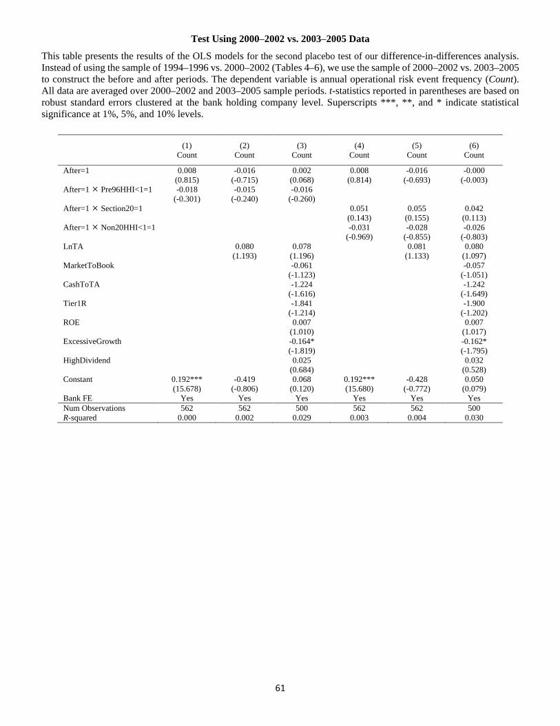
61
Test Using 2000–2002 vs. 2003–2005 Data
This table presents the results of the OLS models for the second placebo test of our difference-in-differences analysis. Instead of using the sample of 1994–1996 vs. 2000–2002 (Tables 4–6), we use the sample of 2000–2002 vs. 2003–2005 to construct the before and after periods. The dependent variable is annual operational risk event frequency (Count). All data are averaged over 2000–2002 and 2003–2005 sample periods. t-statistics reported in parentheses are based on robust standard errors clustered at the bank holding company level. Superscripts ***, **, and * indicate statistical significance at 1%, 5%, and 10% levels.
(1) (2) (3) (4) (5) (6) Count Count Count Count Count Count
After=1 0.008 -0.016 0.002 0.008 -0.016 -0.000 (0.815) (-0.715) (0.068) (0.814) (-0.693) (-0.003) After=1 Pre96HHI<1=1 -0.018 -0.015 -0.016 (-0.301) (-0.240) (-0.260) After=1 Section20=1 0.051 0.055 0.042 (0.143) (0.155) (0.113) After=1 Non20HHI<1=1 -0.031 -0.028 -0.026 (-0.969) (-0.855) (-0.803) LnTA 0.080 0.078 0.081 0.080 (1.193) (1.196) (1.133) (1.097) MarketToBook -0.061 -0.057 (-1.123) (-1.051) CashToTA -1.224 -1.242 (-1.616) (-1.649) Tier1R -1.841 -1.900 (-1.214) (-1.202) ROE 0.007 0.007 (1.010) (1.017) ExcessiveGrowth -0.164* -0.162* (-1.819) (-1.795) HighDividend 0.025 0.032 (0.684) (0.528) Constant 0.192*** -0.419 0.068 0.192*** -0.428 0.050 (15.678) (-0.806) (0.120) (15.680) (-0.772) (0.079) Bank FE Yes Yes Yes Yes Yes Yes Num Observations 562 562 500 562 562 500 R-squared 0.000 0.002 0.029 0.003 0.004 0.030
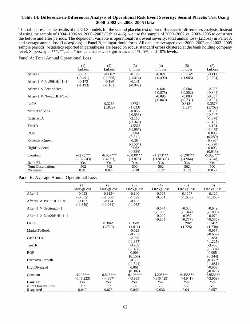
62
Table 14: Difference-in-Differences Analysis of Operational Risk Event Severity: Second Placebo Test Using 2000–2002 vs. 2003–2005 Data
This table presents the results of the OLS models for the second placebo test of our difference-in-differences analysis. Instead of using the sample of 1994–1996 vs. 2000–2002 (Tables 4–6), we use the sample of 2000–2002 vs. 2003–2005 to construct the before and after periods. The dependent variable is operational risk event severity: total annual loss (LnLoss) in Panel A and average annual loss (LnAvgLoss) in Panel B, in logarithmic form. All data are averaged over 2000–2002 and 2003–2005 sample periods. t-statistics reported in parentheses are based on robust standard errors clustered at the bank holding company level. Superscripts ***, **, and * indicate statistical significance at 1%, 5%, and 10% levels. Panel A: Total Annual Operational Loss
(1) (2) (3) (4) (5) (6) LnLoss LnLoss LnLoss LnLoss LnLoss LnLoss After=1 -0.021 -0.116* -0.129 -0.021 -0.114* -0.111 (-0.491) (-1.696) (-1.414) (-0.490) (-1.685) (-1.204) After=1 Pre96HHI<1=1 -0.173 -0.160 -0.141 (-1.193) (-1.101) (-0.942) After=1 Section20=1 -0.601 -0.584 -0.587 (-0.875) (-0.852) (-0.841) After=1 Non20HHI<1=1 -0.096 -0.083 -0.067 (-0.843) (-0.731) (-0.551) LnTA 0.326* 0.373* 0.318* 0.357* (1.829) (1.833) (1.827) (1.762) MarketToBook -0.056 -0.087 (-0.558) (-0.947) CashToTA -2.110 -1.978 (-1.340) (-1.187) Tier1R -4.556* -4.104 (-1.667) (-1.479) ROE 0.004 0.006 (0.211) (0.289) ExcessiveGrowth -0.364 -0.380* (-1.594) (-1.720) HighDividend 0.062 0.003 (0.384) (0.015) Constant -4.173*** -6.657*** -6.030*** -4.173*** -6.598*** -5.893*** (-137.543) (-4.903) (-3.873) (-138.303) (-4.964) (-3.848) Bank FE Yes Yes Yes Yes Yes Yes Num Observations 562 562 500 562 562 500 R-squared 0.015 0.020 0.038 0.027 0.032 0.050
Panel B: Average Annual Operational Loss
(1) (2) (3) (4) (5) (6) LnAvgLoss LnAvgLoss LnAvgLoss LnAvgLoss LnAvgLoss LnAvgLoss After=1 -0.023 -0.112* -0.140 -0.023 -0.110* -0.120 (-0.555) (-1.666) (-1.599) (-0.554) (-1.653) (-1.365) After=1 Pre96HHI<1=1 -0.187 -0.174 -0.153 (-1.350) (-1.261) (-1.065) After=1 Section20=1 -0.674 -0.658 -0.649 (-1.065) (-1.044) (-1.009) After=1 Non20HHI<1=1 -0.099 -0.087 -0.070 (-0.884) (-0.777) (-0.586) LnTA 0.304* 0.358* 0.296* 0.341* (1.729) (1.811) (1.726) (1.738) MarketToBook -0.023 -0.057 (-0.237) (-0.637) CashToTA -2.028 -1.881 (-1.387) (-1.225) Tier1R -3.959 -3.455 (-1.488) (-1.304) ROE 0.003 0.005 (0.150) (0.244) ExcessiveGrowth -0.332 -0.350* (-1.541) (-1.681) HighDividend 0.061 -0.005 (0.382) (-0.029) Constant -4.205*** -6.525*** -6.108*** -4.205*** -6.458*** -5.956*** (-145.223) (-4.867) (-3.995) (-146.425) (-4.941) (-3.969) Bank FE Yes Yes Yes Yes Yes Yes Num Observations 562 562 500 562 562 500 R-squared 0.019 0.023 0.040 0.036 0.041 0.057
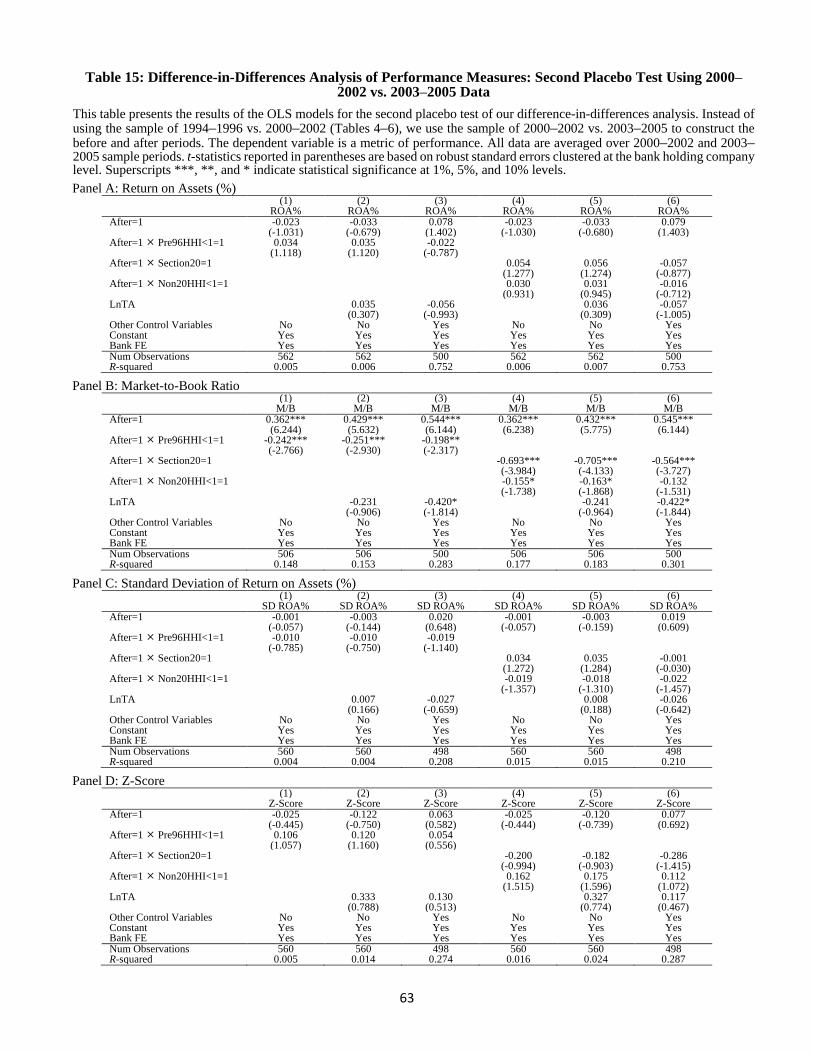
63
Table 15: Difference-in-Differences Analysis of Performance Measures: Second Placebo Test Using 2000–
2002 vs. 2003–2005 Data This table presents the results of the OLS models for the second placebo test of our difference-in-differences analysis. Instead of using the sample of 1994–1996 vs. 2000–2002 (Tables 4–6), we use the sample of 2000–2002 vs. 2003–2005 to construct the before and after periods. The dependent variable is a metric of performance. All data are averaged over 2000–2002 and 2003–2005 sample periods. t-statistics reported in parentheses are based on robust standard errors clustered at the bank holding company level. Superscripts ***, **, and * indicate statistical significance at 1%, 5%, and 10% levels. Panel A: Return on Assets (%)
(1) (2) (3) (4) (5) (6) ROA% ROA% ROA% ROA% ROA% ROA% After=1 -0.023 -0.033 0.078 -0.023 -0.033 0.079 (-1.031) (-0.679) (1.402) (-1.030) (-0.680) (1.403) After=1 Pre96HHI<1=1 0.034 0.035 -0.022 (1.118) (1.120) (-0.787) After=1 Section20=1 0.054 0.056 -0.057 (1.277) (1.274) (-0.877) After=1 Non20HHI<1=1 0.030 0.031 -0.016 (0.931) (0.945) (-0.712) LnTA 0.035 -0.056 0.036 -0.057 (0.307) (-0.993) (0.309) (-1.005) Other Control Variables No No Yes No No Yes Constant Yes Yes Yes Yes Yes Yes Bank FE Yes Yes Yes Yes Yes Yes Num Observations 562 562 500 562 562 500 R-squared 0.005 0.006 0.752 0.006 0.007 0.753
Panel B: Market-to-Book Ratio (1) (2) (3) (4) (5) (6) M/B M/B M/B M/B M/B M/B After=1 0.362*** 0.429*** 0.544*** 0.362*** 0.432*** 0.545*** (6.244) (5.632) (6.144) (6.238) (5.775) (6.144) After=1 Pre96HHI<1=1 -0.242*** -0.251*** -0.198** (-2.766) (-2.930) (-2.317) After=1 Section20=1 -0.693*** -0.705*** -0.564*** (-3.984) (-4.133) (-3.727) After=1 Non20HHI<1=1 -0.155* -0.163* -0.132 (-1.738) (-1.868) (-1.531) LnTA -0.231 -0.420* -0.241 -0.422* (-0.906) (-1.814) (-0.964) (-1.844) Other Control Variables No No Yes No No Yes Constant Yes Yes Yes Yes Yes Yes Bank FE Yes Yes Yes Yes Yes Yes Num Observations 506 506 500 506 506 500 R-squared 0.148 0.153 0.283 0.177 0.183 0.301
Panel C: Standard Deviation of Return on Assets (%) (1) (2) (3) (4) (5) (6) SD ROA% SD ROA% SD ROA% SD ROA% SD ROA% SD ROA% After=1 -0.001 -0.003 0.020 -0.001 -0.003 0.019 (-0.057) (-0.144) (0.648) (-0.057) (-0.159) (0.609) After=1 Pre96HHI<1=1 -0.010 -0.010 -0.019 (-0.785) (-0.750) (-1.140) After=1 Section20=1 0.034 0.035 -0.001 (1.272) (1.284) (-0.030) After=1 Non20HHI<1=1 -0.019 -0.018 -0.022 (-1.357) (-1.310) (-1.457) LnTA 0.007 -0.027 0.008 -0.026 (0.166) (-0.659) (0.188) (-0.642) Other Control Variables No No Yes No No Yes Constant Yes Yes Yes Yes Yes Yes Bank FE Yes Yes Yes Yes Yes Yes Num Observations 560 560 498 560 560 498 R-squared 0.004 0.004 0.208 0.015 0.015 0.210
Panel D: Z-Score (1) (2) (3) (4) (5) (6) Z-Score Z-Score Z-Score Z-Score Z-Score Z-Score After=1 -0.025 -0.122 0.063 -0.025 -0.120 0.077 (-0.445) (-0.750) (0.582) (-0.444) (-0.739) (0.692) After=1 Pre96HHI<1=1 0.106 0.120 0.054 (1.057) (1.160) (0.556) After=1 Section20=1 -0.200 -0.182 -0.286 (-0.994) (-0.903) (-1.415) After=1 Non20HHI<1=1 0.162 0.175 0.112 (1.515) (1.596) (1.072) LnTA 0.333 0.130 0.327 0.117 (0.788) (0.513) (0.774) (0.467) Other Control Variables No No Yes No No Yes Constant Yes Yes Yes Yes Yes Yes Bank FE Yes Yes Yes Yes Yes Yes Num Observations 560 560 498 560 560 498 R-squared 0.005 0.014 0.274 0.016 0.024 0.287
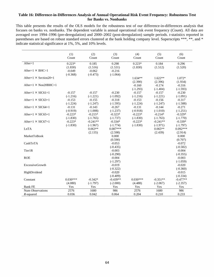
64
Table 16: Difference-in-Differences Analysis of Annual Operational Risk Event Frequency: Robustness Test for Banks vs. Nonbanks
This table presents the results of the OLS models for the robustness test of our difference-in-differences analysis that focuses on banks vs. nonbanks. The dependent variable is annual operational risk event frequency (Count). All data are averaged over 1994–1996 (pre-deregulation) and 2000–2002 (post-deregulation) sample periods. t-statistics reported in parentheses are based on robust standard errors clustered at the bank holding company level. Superscripts ***, **, and * indicate statistical significance at 1%, 5%, and 10% levels.
(1) (2) (3) (4) (5) (6) Count Count Count Count Count Count
After=1 0.223* 0.185 0.298 0.223* 0.184 0.296 (1.830) (1.516) (1.531) (1.830) (1.512) (1.520) After=1 BHC=1 -0.049 -0.062 -0.216 (-0.368) (-0.473) (-1.064) After=1 Section20=1 1.634** 1.622** 1.072* (2.390) (2.396) (1.934) After=1 Non20BHC=1 -0.160 -0.174 -0.316 (-1.293) (-1.404) (-1.593) After=1 SIC61=1 -0.157 -0.157 -0.230 -0.157 -0.157 -0.230 (-1.216) (-1.221) (-1.092) (-1.216) (-1.221) (-1.091) After=1 SIC63=1 -0.153 -0.155 -0.318 -0.153 -0.156 -0.317 (-1.224) (-1.247) (-1.595) (-1.224) (-1.247) (-1.588) After=1 SIC64=1 -0.131 -0.143 -0.267 -0.131 -0.144 -0.271 (-0.919) (-1.008) (-1.237) (-0.918) (-1.010) (-1.251) After=1 SIC65=1 -0.223* -0.215* -0.323* -0.223* -0.214* -0.329* (-1.830) (-1.765) (-1.737) (-1.830) (-1.763) (-1.770) After=1 SIC67=1 -0.223* -0.241** -0.334* -0.223* -0.241** -0.339* (-1.830) (-1.967) (-1.774) (-1.830) (-1.971) (-1.797) LnTA 0.063** 0.087*** 0.065** 0.092*** (2.135) (2.598) (2.439) (2.914) MarketToBook 0.000 0.000 (0.590) (0.707) CashToTA -0.053 -0.072 (-0.435) (-0.582) Tier1R -0.003 -0.004 (-0.290) (-0.355) ROE -0.004 -0.003 (-1.297) (-1.059) ExcessiveGrowth -0.019 -0.020 (-0.322) (-0.360) HighDividend -0.020 -0.015 (-0.409) (-0.334) Constant 0.030*** -0.342* -0.439** 0.030*** -0.351** -0.477**
(4.080) (-1.797) (-2.000) (4.488) (-2.067) (-2.357) Bank FE Yes Yes Yes Yes Yes Yes Num Observations 2576 1680 986 2576 1680 986 R-squared 0.036 0.042 0.064 0.204 0.210 0.233
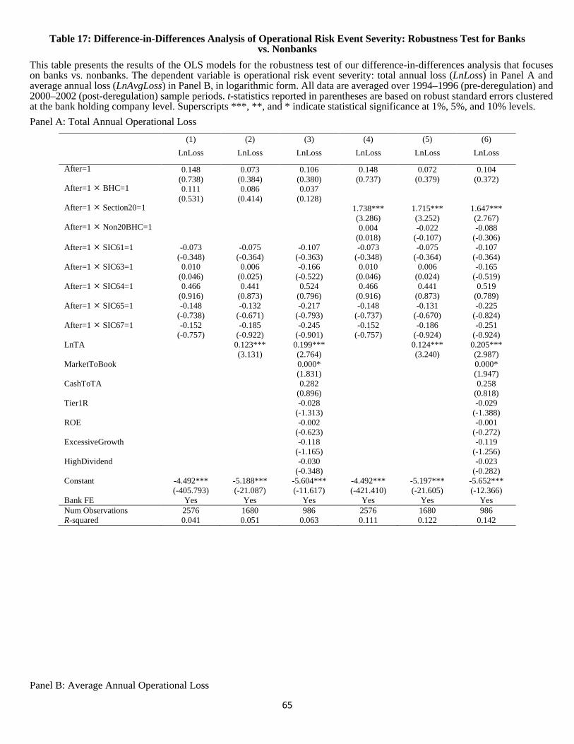
65
Table 17: Difference-in-Differences Analysis of Operational Risk Event Severity: Robustness Test for Banks vs. Nonbanks
This table presents the results of the OLS models for the robustness test of our difference-in-differences analysis that focuses on banks vs. nonbanks. The dependent variable is operational risk event severity: total annual loss (LnLoss) in Panel A and average annual loss (LnAvgLoss) in Panel B, in logarithmic form. All data are averaged over 1994–1996 (pre-deregulation) and 2000–2002 (post-deregulation) sample periods. t-statistics reported in parentheses are based on robust standard errors clustered at the bank holding company level. Superscripts ***, **, and * indicate statistical significance at 1%, 5%, and 10% levels. Panel A: Total Annual Operational Loss
(1) (2) (3) (4) (5) (6)
LnLoss LnLoss LnLoss LnLoss LnLoss LnLoss
After=1 0.148 0.073 0.106 0.148 0.072 0.104 (0.738) (0.384) (0.380) (0.737) (0.379) (0.372) After=1 BHC=1 0.111 0.086 0.037 (0.531) (0.414) (0.128) After=1 Section20=1 1.738*** 1.715*** 1.647*** (3.286) (3.252) (2.767) After=1 Non20BHC=1 0.004 -0.022 -0.088 (0.018) (-0.107) (-0.306) After=1 SIC61=1 -0.073 -0.075 -0.107 -0.073 -0.075 -0.107 (-0.348) (-0.364) (-0.363) (-0.348) (-0.364) (-0.364) After=1 SIC63=1 0.010 0.006 -0.166 0.010 0.006 -0.165 (0.046) (0.025) (-0.522) (0.046) (0.024) (-0.519) After=1 SIC64=1 0.466 0.441 0.524 0.466 0.441 0.519 (0.916) (0.873) (0.796) (0.916) (0.873) (0.789) After=1 SIC65=1 -0.148 -0.132 -0.217 -0.148 -0.131 -0.225 (-0.738) (-0.671) (-0.793) (-0.737) (-0.670) (-0.824) After=1 SIC67=1 -0.152 -0.185 -0.245 -0.152 -0.186 -0.251 (-0.757) (-0.922) (-0.901) (-0.757) (-0.924) (-0.924) LnTA 0.123*** 0.199*** 0.124*** 0.205*** (3.131) (2.764) (3.240) (2.987) MarketToBook 0.000* 0.000* (1.831) (1.947) CashToTA 0.282 0.258 (0.896) (0.818) Tier1R -0.028 -0.029 (-1.313) (-1.388) ROE -0.002 -0.001 (-0.623) (-0.272) ExcessiveGrowth -0.118 -0.119 (-1.165) (-1.256) HighDividend -0.030 -0.023 (-0.348) (-0.282) Constant -4.492*** -5.188*** -5.604*** -4.492*** -5.197*** -5.652***
(-405.793) (-21.087) (-11.617) (-421.410) (-21.605) (-12.366) Bank FE Yes Yes Yes Yes Yes Yes Num Observations 2576 1680 986 2576 1680 986 R-squared 0.041 0.051 0.063 0.111 0.122 0.142
Panel B: Average Annual Operational Loss
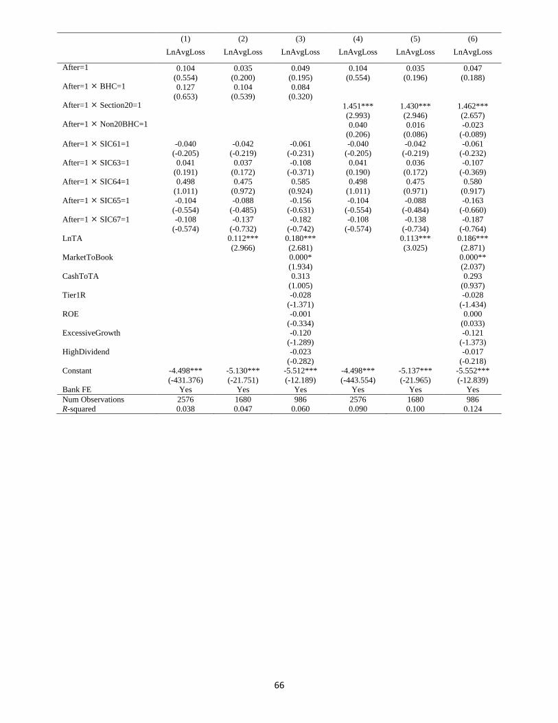
66
(1) (2) (3) (4) (5) (6)
LnAvgLoss LnAvgLoss LnAvgLoss LnAvgLoss LnAvgLoss LnAvgLoss
After=1 0.104 0.035 0.049 0.104 0.035 0.047 (0.554) (0.200) (0.195) (0.554) (0.196) (0.188) After=1 BHC=1 0.127 0.104 0.084 (0.653) (0.539) (0.320) After=1 Section20=1 1.451*** 1.430*** 1.462*** (2.993) (2.946) (2.657) After=1 Non20BHC=1 0.040 0.016 -0.023 (0.206) (0.086) (-0.089) After=1 SIC61=1 -0.040 -0.042 -0.061 -0.040 -0.042 -0.061 (-0.205) (-0.219) (-0.231) (-0.205) (-0.219) (-0.232) After=1 SIC63=1 0.041 0.037 -0.108 0.041 0.036 -0.107 (0.191) (0.172) (-0.371) (0.190) (0.172) (-0.369) After=1 SIC64=1 0.498 0.475 0.585 0.498 0.475 0.580 (1.011) (0.972) (0.924) (1.011) (0.971) (0.917) After=1 SIC65=1 -0.104 -0.088 -0.156 -0.104 -0.088 -0.163 (-0.554) (-0.485) (-0.631) (-0.554) (-0.484) (-0.660) After=1 SIC67=1 -0.108 -0.137 -0.182 -0.108 -0.138 -0.187 (-0.574) (-0.732) (-0.742) (-0.574) (-0.734) (-0.764) LnTA 0.112*** 0.180*** 0.113*** 0.186*** (2.966) (2.681) (3.025) (2.871) MarketToBook 0.000* 0.000** (1.934) (2.037) CashToTA 0.313 0.293 (1.005) (0.937) Tier1R -0.028 -0.028 (-1.371) (-1.434) ROE -0.001 0.000 (-0.334) (0.033) ExcessiveGrowth -0.120 -0.121 (-1.289) (-1.373) HighDividend -0.023 -0.017 (-0.282) (-0.218) Constant -4.498*** -5.130*** -5.512*** -4.498*** -5.137*** -5.552***
(-431.376) (-21.751) (-12.189) (-443.554) (-21.965) (-12.839) Bank FE Yes Yes Yes Yes Yes Yes Num Observations 2576 1680 986 2576 1680 986 R-squared 0.038 0.047 0.060 0.090 0.100 0.124

APPENDIX
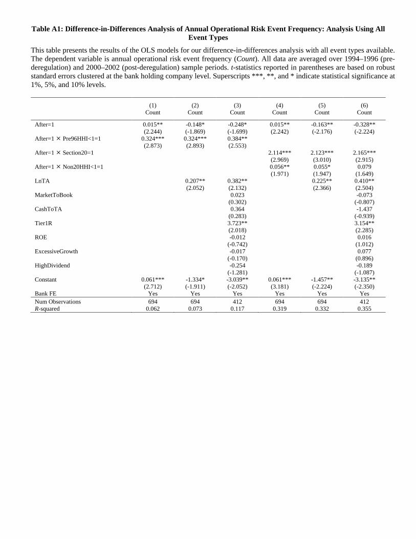
Table A1: Difference-in-Differences Analysis of Annual Operational Risk Event Frequency: Analysis Using All Event Types
This table presents the results of the OLS models for our difference-in-differences analysis with all event types available. The dependent variable is annual operational risk event frequency (Count). All data are averaged over 1994–1996 (pre-deregulation) and 2000–2002 (post-deregulation) sample periods. t-statistics reported in parentheses are based on robust standard errors clustered at the bank holding company level. Superscripts ***, **, and * indicate statistical significance at 1%, 5%, and 10% levels.
(1) (2) (3) (4) (5) (6) Count Count Count Count Count Count
After=1 0.015** -0.148* -0.248* 0.015** -0.163** -0.328** (2.244) (-1.869) (-1.699) (2.242) (-2.176) (-2.224) After=1 Pre96HHI<1=1 0.324*** 0.324*** 0.384** (2.873) (2.893) (2.553) After=1 Section20=1 2.114*** 2.123*** 2.165*** (2.969) (3.010) (2.915) After=1 Non20HHI<1=1 0.056** 0.055* 0.079 (1.971) (1.947) (1.649) LnTA 0.207** 0.382** 0.225** 0.410** (2.052) (2.132) (2.366) (2.504) MarketToBook 0.023 -0.073 (0.302) (-0.807) CashToTA 0.364 -1.437 (0.283) (-0.939) Tier1R 3.723** 3.154** (2.018) (2.285) ROE -0.012 0.016 (-0.742) (1.012) ExcessiveGrowth -0.017 0.077 (-0.170) (0.896) HighDividend -0.254 -0.189 (-1.281) (-1.087) Constant 0.061*** -1.334* -3.039** 0.061*** -1.457** -3.135** (2.712) (-1.911) (-2.052) (3.181) (-2.224) (-2.350) Bank FE Yes Yes Yes Yes Yes Yes Num Observations 694 694 412 694 694 412 R-squared 0.062 0.073 0.117 0.319 0.332 0.355
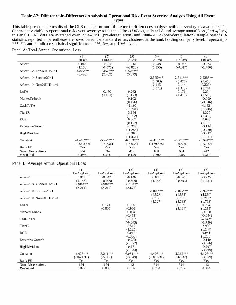
Table A2: Difference-in-Differences Analysis of Operational Risk Event Severity: Analysis Using All Event Types
This table presents the results of the OLS models for our difference-in-differences analysis with all event types available. The dependent variable is operational risk event severity: total annual loss (LnLoss) in Panel A and average annual loss (LnAvgLoss) in Panel B. All data are averaged over 1994–1996 (pre-deregulation) and 2000–2002 (post-deregulation) sample periods. t-statistics reported in parentheses are based on robust standard errors clustered at the bank holding company level. Superscripts ***, **, and * indicate statistical significance at 1%, 5%, and 10% levels. Panel A: Total Annual Operational Loss
(1) (2) (3) (4) (5) (6) LnLoss LnLoss LnLoss LnLoss LnLoss LnLoss After=1 0.048 -0.070 -0.181 0.048 -0.087 -0.274 (1.156) (-0.575) (-0.828) (1.155) (-0.817) (-1.480) After=1 Pre96HHI<1=1 0.456*** 0.457*** 0.576*** (3.426) (3.433) (3.879) After=1 Section20=1 2.535*** 2.541*** 2.638*** (5.083) (5.076) (5.410) After=1 Non20HHI<1=1 0.145 0.144 0.223* (1.371) (1.379) (1.764) LnTA 0.150 0.262 0.171 0.294 (1.051) (1.173) (1.416) (1.508) MarketToBook 0.102 -0.009 (0.476) (-0.046) CashToTA -2.107 -4.193* (-0.734) (-1.745) Tier1R 3.984 3.325 (1.302) (1.352) ROE 0.007 0.040 (0.177) (1.195) ExcessiveGrowth -0.233 -0.124 (-1.253) (-0.730) HighDividend -0.307 -0.232 (-1.431) (-1.051) Constant -4.413*** -5.427*** -6.513*** -4.413*** -5.570*** -6.624*** (-156.879) (-5.636) (-3.535) (-179.339) (-6.806) (-3.932) Bank FE Yes Yes Yes Yes Yes Yes Num Observations 694 694 412 694 694 412 R-squared 0.086 0.090 0.149 0.302 0.307 0.362
Panel B: Average Annual Operational Loss
(1) (2) (3) (4) (5) (6) LnAvgLoss LnAvgLoss LnAvgLoss LnAvgLoss LnAvgLoss LnAvgLoss After=1 0.048 -0.047 -0.146 0.048 -0.061 -0.225 (1.156) (-0.405) (-0.699) (1.155) (-0.593) (-1.237) After=1 Pre96HHI<1=1 0.400*** 0.400*** 0.513*** (3.214) (3.219) (3.672) After=1 Section20=1 2.161*** 2.165*** 2.267*** (4.578) (4.561) (4.869) After=1 Non20HHI<1=1 0.136 0.135 0.212* (1.327) (1.333) (1.713) LnTA 0.121 0.207 0.139 0.234 (0.899) (0.992) (1.194) (1.255) MarketToBook 0.084 -0.010 (0.411) (-0.054) CashToTA -2.367 -4.142* (-0.843) (-1.730) Tier1R 3.517 2.956 (1.225) (1.244) ROE 0.013 0.041 (0.355) (1.255) ExcessiveGrowth -0.233 -0.140 (-1.372) (-0.866) HighDividend -0.271 -0.207 (-1.344) (-0.999) Constant -4.426*** -5.241*** -6.081*** -4.426*** -5.362*** -6.176*** (-167.091) (-5.801) (-3.549) (-185.631) (-6.832) (-3.859) Bank FE Yes Yes Yes Yes Yes Yes Num Observations 694 694 412 694 694 412 R-squared 0.077 0.080 0.137 0.254 0.257 0.314
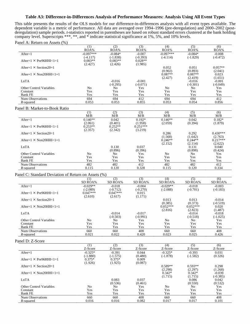
Table A3: Difference-in-Differences Analysis of Performance Measures: Analysis Using All Event Types This table presents the results of the OLS models for our difference-in-differences analysis with all event types available. The dependent variable is a metric of performance. All data are averaged over 1994–1996 (pre-deregulation) and 2000–2002 (post-deregulation) sample periods. t-statistics reported in parentheses are based on robust standard errors clustered at the bank holding company level. Superscripts ***, **, and * indicate statistical significance at 1%, 5%, and 10% levels. Panel A: Return on Assets (%)
(1) (2) (3) (4) (5) (6) ROA% ROA% ROA% ROA% ROA% ROA% After=1 -0.097*** -0.084* -0.007 -0.097*** -0.084* -0.008 (-4.117) (-1.838) (-0.393) (-4.114) (-1.829) (-0.472) After=1 Pre96HHI<1=1 0.083** 0.083** 0.028** (2.427) (2.426) (1.985) After=1 Section20=1 0.052 0.051 0.057** (0.902) (0.893) (2.041) After=1 Non20HHI<1=1 0.087** 0.087** 0.023 (2.427) (2.419) (1.651) LnTA -0.016 -0.001 -0.016 -0.001 (-0.295) (-0.071) (-0.301) (-0.049) Other Control Variables No No Yes No No Yes Constant Yes Yes Yes Yes Yes Yes Bank FE Yes Yes Yes Yes Yes Yes Num Observations 694 694 412 694 694 412 R-squared 0.053 0.053 0.855 0.053 0.054 0.856
Panel B: Market-to-Book Ratio (1) (2) (3) (4) (5) (6) M/B M/B M/B M/B M/B M/B After=1 0.146** 0.042 0.192* 0.146** 0.042 0.182* (2.061) (0.401) (1.958) (2.059) (0.394) (1.879) After=1 Pre96HHI<1=1 0.253** 0.252** 0.251*** (2.357) (2.342) (3.219) After=1 Section20=1 0.286 0.292 0.430*** (1.568) (1.642) (2.763) After=1 Non20HHI<1=1 0.246** 0.244** 0.217*** (2.152) (2.114) (2.622) LnTA 0.130 0.037 0.131 0.040 (0.896) (0.396) (0.898) (0.424) Other Control Variables No No Yes No No Yes Constant Yes Yes Yes Yes Yes Yes Bank FE Yes Yes Yes Yes Yes Yes Num Observations 482 482 412 482 482 412 R-squared 0.115 0.120 0.328 0.115 0.120 0.334
Panel C: Standard Deviation of Return on Assets (%) (1) (2) (3) (4) (5) (6) SD ROA% SD ROA% SD ROA% SD ROA% SD ROA% SD ROA% After=1 -0.029** -0.018 -0.004 -0.029** -0.018 -0.003 (-2.089) (-0.712) (-0.270) (-2.088) (-0.701) (-0.183) After=1 Pre96HHI<1=1 0.047*** 0.047*** 0.015 (2.610) (2.617) (1.171) After=1 Section20=1 0.013 0.013 -0.014 (0.385) (0.373) (-0.519) After=1 Non20HHI<1=1 0.052*** 0.052*** 0.020 (2.816) (2.823) (1.487) LnTA -0.014 -0.017 -0.014 -0.018 (-0.503) (-0.991) (-0.518) (-1.025) Other Control Variables No No Yes No No Yes Constant Yes Yes Yes Yes Yes Yes Bank FE Yes Yes Yes Yes Yes Yes Num Observations 660 660 408 660 660 408 R-squared 0.021 0.022 0.420 0.023 0.025 0.426
Panel D: Z-Score (1) (2) (3) (4) (5) (6) Z-Score Z-Score Z-Score Z-Score Z-Score Z-Score After=1 -0.325* -0.391 0.044 -0.325* -0.393 0.031 (-1.880) (-1.575) (0.480) (-1.878) (-1.582) (0.326) After=1 Pre96HHI<1=1 0.375* 0.375* 0.009 (1.926) (1.925) (0.087) After=1 Section20=1 0.589** 0.593** 0.298 (2.298) (2.297) (1.268) After=1 Non20HHI<1=1 0.342* 0.342* -0.039 (1.715) (1.715) (-0.385) LnTA 0.083 0.037 0.086 0.042 (0.536) (0.461) (0.550) (0.532) Other Control Variables No No Yes No No Yes Constant Yes Yes Yes Yes Yes Yes Bank FE Yes Yes Yes Yes Yes Yes Num Observations 660 660 408 660 660 408 R-squared 0.016 0.016 0.082 0.017 0.017 0.101
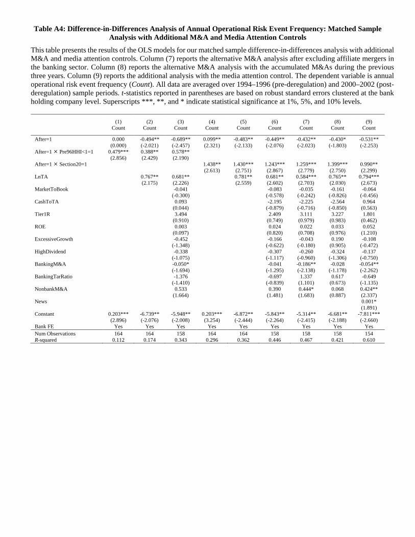
Table A4: Difference-in-Differences Analysis of Annual Operational Risk Event Frequency: Matched Sample Analysis with Additional M&A and Media Attention Controls
This table presents the results of the OLS models for our matched sample difference-in-differences analysis with additional M&A and media attention controls. Column (7) reports the alternative M&A analysis after excluding affiliate mergers in the banking sector. Column (8) reports the alternative M&A analysis with the accumulated M&As during the previous three years. Column (9) reports the additional analysis with the media attention control. The dependent variable is annual operational risk event frequency (Count). All data are averaged over 1994–1996 (pre-deregulation) and 2000–2002 (post-deregulation) sample periods. t-statistics reported in parentheses are based on robust standard errors clustered at the bank holding company level. Superscripts ***, **, and * indicate statistical significance at 1%, 5%, and 10% levels.
(1) (2) (3) (4) (5) (6) (7) (8) (9) Count Count Count Count Count Count Count Count Count
After=1 0.000 -0.494** -0.689** 0.099** -0.483** -0.449** -0.432** -0.430* -0.531** (0.000) (-2.021) (-2.457) (2.321) (-2.133) (-2.076) (-2.023) (-1.803) (-2.253) After=1 Pre96HHI<1=1 0.479*** 0.388** 0.578** (2.856) (2.429) (2.190) After=1 Section20=1 1.438** 1.430*** 1.243*** 1.259*** 1.399*** 0.990** (2.613) (2.751) (2.867) (2.779) (2.750) (2.299) LnTA 0.767** 0.681** 0.781** 0.681** 0.584*** 0.765** 0.794*** (2.175) (2.226) (2.559) (2.602) (2.703) (2.030) (2.673) MarketToBook -0.041 -0.083 -0.035 -0.161 -0.064 (-0.300) (-0.578) (-0.242) (-0.826) (-0.456) CashToTA 0.093 -2.195 -2.225 -2.564 0.964 (0.044) (-0.879) (-0.716) (-0.850) (0.563) Tier1R 3.494 2.409 3.111 3.227 1.801 (0.910) (0.749) (0.979) (0.983) (0.462) ROE 0.003 0.024 0.022 0.033 0.052 (0.097) (0.820) (0.708) (0.976) (1.210) ExcessiveGrowth -0.452 -0.166 -0.043 0.190 -0.108 (-1.348) (-0.622) (-0.180) (0.905) (-0.472) HighDividend -0.338 -0.307 -0.260 -0.324 -0.137 (-1.075) (-1.117) (-0.960) (-1.306) (-0.750) BankingM&A -0.050* -0.041 -0.186** -0.028 -0.054** (-1.694) (-1.295) (-2.138) (-1.178) (-2.262) BankingTarRatio -1.376 -0.697 1.337 0.617 -0.649 (-1.410) (-0.839) (1.101) (0.673) (-1.135) NonbankM&A 0.533 0.390 0.444* 0.068 0.424** (1.664) (1.481) (1.683) (0.887) (2.337) News 0.001* (1.891) Constant 0.203*** -6.739** -5.948** 0.203*** -6.872** -5.843** -5.314** -6.681** -7.811*** (2.896) (-2.076) (-2.008) (3.254) (-2.444) (-2.264) (-2.415) (-2.188) (-2.660) Bank FE Yes Yes Yes Yes Yes Yes Yes Yes Yes Num Observations 164 164 158 164 164 158 158 158 154 R-squared 0.112 0.174 0.343 0.296 0.362 0.446 0.467 0.421 0.610
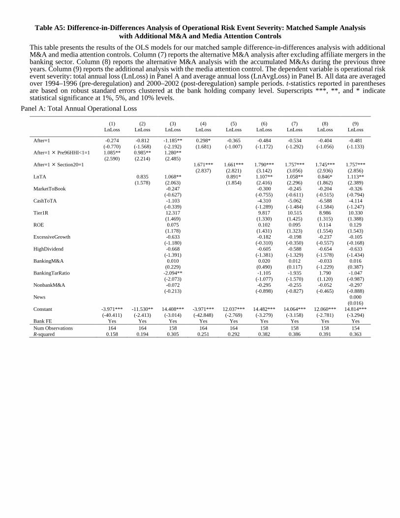
Table A5: Difference-in-Differences Analysis of Operational Risk Event Severity: Matched Sample Analysis with Additional M&A and Media Attention Controls
This table presents the results of the OLS models for our matched sample difference-in-differences analysis with additional M&A and media attention controls. Column (7) reports the alternative M&A analysis after excluding affiliate mergers in the banking sector. Column (8) reports the alternative M&A analysis with the accumulated M&As during the previous three years. Column (9) reports the additional analysis with the media attention control. The dependent variable is operational risk event severity: total annual loss (LnLoss) in Panel A and average annual loss (LnAvgLoss) in Panel B. All data are averaged over 1994–1996 (pre-deregulation) and 2000–2002 (post-deregulation) sample periods. t-statistics reported in parentheses are based on robust standard errors clustered at the bank holding company level. Superscripts ***, **, and * indicate statistical significance at 1%, 5%, and 10% levels.
Panel A: Total Annual Operational Loss
(1) (2) (3) (4) (5) (6) (7) (8) (9) LnLoss LnLoss LnLoss LnLoss LnLoss LnLoss LnLoss LnLoss LnLoss
After=1 -0.274 -0.812 -1.185** 0.298* -0.365 -0.484 -0.534 -0.404 -0.481 (-0.770) (-1.568) (-2.192) (1.681) (-1.007) (-1.172) (-1.292) (-1.056) (-1.133) After=1 Pre96HHI<1=1 1.085** 0.985** 1.280** (2.590) (2.214) (2.485) After=1 Section20=1 1.671*** 1.661*** 1.790*** 1.757*** 1.745*** 1.757*** (2.837) (2.821) (3.142) (3.056) (2.936) (2.856) LnTA 0.835 1.068** 0.891* 1.107** 1.058** 0.846* 1.113** (1.578) (2.063) (1.854) (2.416) (2.296) (1.862) (2.389) MarketToBook -0.247 -0.300 -0.245 -0.204 -0.326 (-0.627) (-0.755) (-0.611) (-0.515) (-0.794) CashToTA -1.103 -4.310 -5.062 -6.588 -4.114 (-0.339) (-1.289) (-1.484) (-1.584) (-1.247) Tier1R 12.317 9.817 10.515 8.986 10.330 (1.469) (1.330) (1.425) (1.315) (1.388) ROE 0.075 0.102 0.095 0.114 0.129 (1.178) (1.431) (1.323) (1.554) (1.543) ExcessiveGrowth -0.633 -0.182 -0.198 -0.237 -0.105 (-1.180) (-0.310) (-0.350) (-0.557) (-0.168) HighDividend -0.668 -0.605 -0.588 -0.654 -0.633 (-1.391) (-1.381) (-1.329) (-1.578) (-1.434) BankingM&A 0.010 0.020 0.012 -0.033 0.016 (0.229) (0.490) (0.117) (-1.229) (0.387) BankingTarRatio -2.094** -1.105 -1.935 1.790 -1.047 (-2.073) (-1.077) (-1.570) (1.120) (-0.987) NonbankM&A -0.072 -0.295 -0.255 -0.052 -0.297 (-0.213) (-0.898) (-0.827) (-0.465) (-0.888) News 0.000 (0.016) Constant -3.971*** -11.530** 14.408*** -3.971*** 12.037*** 14.482*** 14.064*** 12.060*** 14.814*** (-40.411) (-2.413) (-3.014) (-42.848) (-2.769) (-3.279) (-3.158) (-2.781) (-3.294) Bank FE Yes Yes Yes Yes Yes Yes Yes Yes Yes Num Observations 164 164 158 164 164 158 158 158 154 R-squared 0.158 0.194 0.305 0.251 0.292 0.382 0.386 0.391 0.363
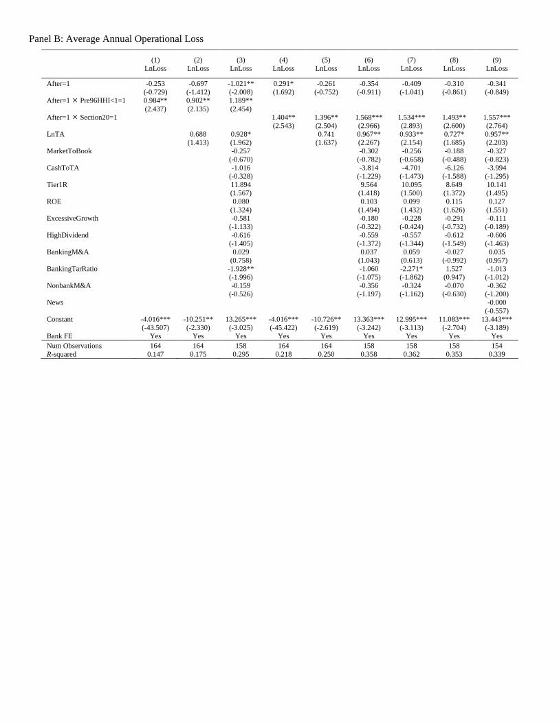
Panel B: Average Annual Operational Loss
(1) (2) (3) (4) (5) (6) (7) (8) (9) LnLoss LnLoss LnLoss LnLoss LnLoss LnLoss LnLoss LnLoss LnLoss
After=1 -0.253 -0.697 -1.021** 0.291* -0.261 -0.354 -0.409 -0.310 -0.341 (-0.729) (-1.412) (-2.008) (1.692) (-0.752) (-0.911) (-1.041) (-0.861) (-0.849) After=1 Pre96HHI<1=1 0.984** 0.902** 1.189** (2.437) (2.135) (2.454) After=1 Section20=1 1.404** 1.396** 1.568*** 1.534*** 1.493** 1.557*** (2.543) (2.504) (2.966) (2.893) (2.600) (2.764) LnTA 0.688 0.928* 0.741 0.967** 0.933** 0.727* 0.957** (1.413) (1.962) (1.637) (2.267) (2.154) (1.685) (2.203) MarketToBook -0.257 -0.302 -0.256 -0.188 -0.327 (-0.670) (-0.782) (-0.658) (-0.488) (-0.823) CashToTA -1.016 -3.814 -4.701 -6.126 -3.994 (-0.328) (-1.229) (-1.473) (-1.588) (-1.295) Tier1R 11.894 9.564 10.095 8.649 10.141 (1.567) (1.418) (1.500) (1.372) (1.495) ROE 0.080 0.103 0.099 0.115 0.127 (1.324) (1.494) (1.432) (1.626) (1.551) ExcessiveGrowth -0.581 -0.180 -0.228 -0.291 -0.111 (-1.133) (-0.322) (-0.424) (-0.732) (-0.189) HighDividend -0.616 -0.559 -0.557 -0.612 -0.606 (-1.405) (-1.372) (-1.344) (-1.549) (-1.463) BankingM&A 0.029 0.037 0.059 -0.027 0.035 (0.758) (1.043) (0.613) (-0.992) (0.957) BankingTarRatio -1.928** -1.060 -2.271* 1.527 -1.013 (-1.996) (-1.075) (-1.862) (0.947) (-1.012) NonbankM&A -0.159 -0.356 -0.324 -0.070 -0.362 (-0.526) (-1.197) (-1.162) (-0.630) (-1.200) News -0.000 (-0.557) Constant -4.016*** -10.251** 13.265*** -4.016*** -10.726** 13.363*** 12.995*** 11.083*** 13.443*** (-43.507) (-2.330) (-3.025) (-45.422) (-2.619) (-3.242) (-3.113) (-2.704) (-3.189) Bank FE Yes Yes Yes Yes Yes Yes Yes Yes Yes Num Observations 164 164 158 164 164 158 158 158 154 R-squared 0.147 0.175 0.295 0.218 0.250 0.358 0.362 0.353 0.339
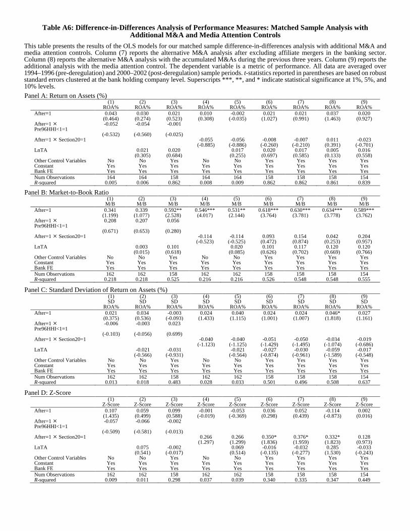
Table A6: Difference-in-Differences Analysis of Performance Measures: Matched Sample Analysis with Additional M&A and Media Attention Controls
This table presents the results of the OLS models for our matched sample difference-in-differences analysis with additional M&A and media attention controls. Column (7) reports the alternative M&A analysis after excluding affiliate mergers in the banking sector. Column (8) reports the alternative M&A analysis with the accumulated M&As during the previous three years. Column (9) reports the additional analysis with the media attention control. The dependent variable is a metric of performance. All data are averaged over 1994–1996 (pre-deregulation) and 2000–2002 (post-deregulation) sample periods. t-statistics reported in parentheses are based on robust standard errors clustered at the bank holding company level. Superscripts ***, **, and * indicate statistical significance at 1%, 5%, and 10% levels. Panel A: Return on Assets (%)
(1) (2) (3) (4) (5) (6) (7) (8) (9) ROA% ROA% ROA% ROA% ROA% ROA% ROA% ROA% ROA% After=1 0.043 0.030 0.021 0.010 -0.002 0.021 0.021 0.037 0.020 (0.464) (0.274) (0.523) (0.308) (-0.035) (1.027) (0.991) (1.463) (0.927) After=1 Pre96HHI<1=1
-0.052 -0.054 -0.001
(-0.532) (-0.560) (-0.025) After=1 Section20=1 -0.055 -0.056 -0.008 -0.007 0.011 -0.023 (-0.885) (-0.886) (-0.260) (-0.210) (0.391) (-0.701) LnTA 0.021 0.020 0.017 0.020 0.017 0.005 0.016 (0.305) (0.684) (0.255) (0.697) (0.585) (0.133) (0.558) Other Control Variables No No Yes No No Yes Yes Yes Yes Constant Yes Yes Yes Yes Yes Yes Yes Yes Yes Bank FE Yes Yes Yes Yes Yes Yes Yes Yes Yes Num Observations 164 164 158 164 164 158 158 158 154 R-squared 0.005 0.006 0.862 0.008 0.009 0.862 0.862 0.861 0.839
Panel B: Market-to-Book Ratio (1) (2) (3) (4) (5) (6) (7) (8) (9) M/B M/B M/B M/B M/B M/B M/B M/B M/B After=1 0.341 0.339 0.592** 0.546*** 0.531** 0.618*** 0.630*** 0.634*** 0.589*** (1.199) (1.077) (2.528) (4.017) (2.144) (3.764) (3.781) (3.778) (3.762) After=1 Pre96HHI<1=1
0.208 0.207 0.056
(0.671) (0.653) (0.280) After=1 Section20=1 -0.114 -0.114 0.093 0.154 0.042 0.204 (-0.523) (-0.525) (0.472) (0.874) (0.253) (0.957) LnTA 0.003 0.101 0.020 0.101 0.117 0.120 0.120 (0.015) (0.618) (0.085) (0.626) (0.702) (0.669) (0.766) Other Control Variables No No Yes No No Yes Yes Yes Yes Constant Yes Yes Yes Yes Yes Yes Yes Yes Yes Bank FE Yes Yes Yes Yes Yes Yes Yes Yes Yes Num Observations 162 162 158 162 162 158 158 158 154 R-squared 0.218 0.218 0.525 0.216 0.216 0.526 0.548 0.548 0.555
Panel C: Standard Deviation of Return on Assets (%) (1) (2) (3) (4) (5) (6) (7) (8) (9) SD
ROA% SD
ROA% SD
ROA% SD
ROA% SD
ROA% SD
ROA% SD
ROA% SD
ROA% SD
ROA% After=1 0.021 0.034 -0.003 0.024 0.040 0.024 0.024 0.046* 0.027 (0.375) (0.536) (-0.093) (1.433) (1.115) (1.001) (1.007) (1.818) (1.161) After=1 Pre96HHI<1=1
-0.006 -0.003 0.023
(-0.103) (-0.056) (0.699) After=1 Section20=1 -0.040 -0.040 -0.051 -0.050 -0.034 -0.019 (-1.123) (-1.125) (-1.429) (-1.495) (-1.074) (-0.686) LnTA -0.021 -0.031 -0.021 -0.027 -0.030 -0.059 -0.017 (-0.566) (-0.931) (-0.564) (-0.874) (-0.961) (-1.589) (-0.548) Other Control Variables No No Yes No No Yes Yes Yes Yes Constant Yes Yes Yes Yes Yes Yes Yes Yes Yes Bank FE Yes Yes Yes Yes Yes Yes Yes Yes Yes Num Observations 162 162 158 162 162 158 158 158 154 R-squared 0.013 0.018 0.483 0.028 0.033 0.501 0.496 0.508 0.637
Panel D: Z-Score (1) (2) (3) (4) (5) (6) (7) (8) (9) Z-Score Z-Score Z-Score Z-Score Z-Score Z-Score Z-Score Z-Score Z-Score After=1 0.107 0.059 0.099 -0.001 -0.053 0.036 0.052 -0.114 0.002 (1.435) (0.499) (0.588) (-0.019) (-0.369) (0.298) (0.439) (-0.873) (0.016) After=1 Pre96HHI<1=1
-0.057 -0.066 -0.002
(-0.509) (-0.581) (-0.013) After=1 Section20=1 0.266 0.266 0.350* 0.376* 0.332* 0.128 (1.297) (1.299) (1.836) (1.959) (1.823) (0.973) LnTA 0.075 -0.002 0.069 -0.016 -0.032 0.285 -0.033 (0.541) (-0.017) (0.514) (-0.135) (-0.277) (1.530) (-0.243) Other Control Variables No No Yes No No Yes Yes Yes Yes Constant Yes Yes Yes Yes Yes Yes Yes Yes Yes Bank FE Yes Yes Yes Yes Yes Yes Yes Yes Yes Num Observations 162 162 158 162 162 158 158 158 154 R-squared 0.009 0.011 0.298 0.037 0.039 0.340 0.335 0.347 0.449
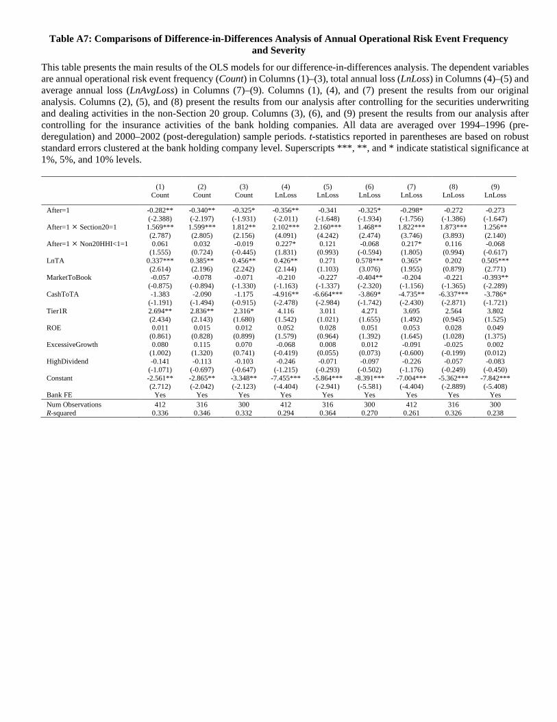
Table A7: Comparisons of Difference-in-Differences Analysis of Annual Operational Risk Event Frequency and Severity
This table presents the main results of the OLS models for our difference-in-differences analysis. The dependent variables are annual operational risk event frequency (Count) in Columns (1)–(3), total annual loss (LnLoss) in Columns (4)–(5) and average annual loss (LnAvgLoss) in Columns (7)–(9). Columns (1), (4), and (7) present the results from our original analysis. Columns (2), (5), and (8) present the results from our analysis after controlling for the securities underwriting and dealing activities in the non-Section 20 group. Columns (3), (6), and (9) present the results from our analysis after controlling for the insurance activities of the bank holding companies. All data are averaged over 1994–1996 (pre-deregulation) and 2000–2002 (post-deregulation) sample periods. t-statistics reported in parentheses are based on robust standard errors clustered at the bank holding company level. Superscripts ***, **, and * indicate statistical significance at 1%, 5%, and 10% levels.
(1) (2) (3) (4) (5) (6) (7) (8) (9) Count Count Count LnLoss LnLoss LnLoss LnLoss LnLoss LnLoss
After=1 -0.282** -0.340** -0.325* -0.356** -0.341 -0.325* -0.298* -0.272 -0.273 (-2.388) (-2.197) (-1.931) (-2.011) (-1.648) (-1.934) (-1.756) (-1.386) (-1.647) After=1 Section20=1 1.569*** 1.599*** 1.812** 2.102*** 2.160*** 1.468** 1.822*** 1.873*** 1.256** (2.787) (2.805) (2.156) (4.091) (4.242) (2.474) (3.746) (3.893) (2.140) After=1 Non20HHI<1=1 0.061 0.032 -0.019 0.227* 0.121 -0.068 0.217* 0.116 -0.068 (1.555) (0.724) (-0.445) (1.831) (0.993) (-0.594) (1.805) (0.994) (-0.617) LnTA 0.337*** 0.385** 0.456** 0.426** 0.271 0.578*** 0.365* 0.202 0.505*** (2.614) (2.196) (2.242) (2.144) (1.103) (3.076) (1.955) (0.879) (2.771) MarketToBook -0.057 -0.078 -0.071 -0.210 -0.227 -0.404** -0.204 -0.221 -0.393** (-0.875) (-0.894) (-1.330) (-1.163) (-1.337) (-2.320) (-1.156) (-1.365) (-2.289) CashToTA -1.383 -2.090 -1.175 -4.916** -6.664*** -3.869* -4.735** -6.337*** -3.786* (-1.191) (-1.494) (-0.915) (-2.478) (-2.984) (-1.742) (-2.430) (-2.871) (-1.721) Tier1R 2.694** 2.836** 2.316* 4.116 3.011 4.271 3.695 2.564 3.802 (2.434) (2.143) (1.680) (1.542) (1.021) (1.655) (1.492) (0.945) (1.525) ROE 0.011 0.015 0.012 0.052 0.028 0.051 0.053 0.028 0.049 (0.861) (0.828) (0.899) (1.579) (0.964) (1.392) (1.645) (1.028) (1.375) ExcessiveGrowth 0.080 0.115 0.070 -0.068 0.008 0.012 -0.091 -0.025 0.002 (1.002) (1.320) (0.741) (-0.419) (0.055) (0.073) (-0.600) (-0.199) (0.012) HighDividend -0.141 -0.113 -0.103 -0.246 -0.071 -0.097 -0.226 -0.057 -0.083 (-1.071) (-0.697) (-0.647) (-1.215) (-0.293) (-0.502) (-1.176) (-0.249) (-0.450) Constant -2.561** -2.865** -3.348** -7.455*** -5.864*** -8.391*** -7.004*** -5.362*** -7.842*** (2.712) (-2.042) (-2.123) (-4.404) (-2.941) (-5.581) (-4.404) (-2.889) (-5.408) Bank FE Yes Yes Yes Yes Yes Yes Yes Yes Yes Num Observations 412 316 300 412 316 300 412 316 300 R-squared 0.336 0.346 0.332 0.294 0.364 0.270 0.261 0.326 0.238