Embed Size (px)
Citation preview

ONLINE APPENDIX∗
BUSINESS CYCLES IN AN OIL ECONOMY
DRAGO BERGHOLTa,§, VEGARD H. LARSENa, AND MARTIN SENECAb
aNORGES BANK bBANK OF ENGLAND
JANUARY 2017
This appendix contains supplementary material not included in the paper. More detailsabout the model are provided in Section A, a description of the data used for estimationin Section B, a robustness analysis using an alternative OECD dataset in Section C, and aset of additional figures and tables referred to in the main text in Section D.
A THE MODEL
The model consists of two country blocks, referred to as home and foreign. With theexception of oil demand, the home block is a small scale version of its foreign counter-part, which represents the rest of the world. Our focus is on the limiting case where thehome economy’s relative size goes to zero, implying that the foreign block approximatesa closed economy. Here, we focus on the part of the home economy that is abstractedfrom in the main text.
A.1 HOUSEHOLDS
Consider household member h ∈ [0, 1] working in sector j ∈ c,m, s (manufacturing,services or oil supply). He maximizes expected lifetime utility, given in period t by
Wj,t(h) = Et∞∑s=t
βs−tZU,s
[(1− χC)ln (Ct(h)− χCCt−1)− χN
Lj,t(h)1+ϕ
1 + ϕ
].
Ct(h) denotes period t consumption while Lj,t(h) denotes hours worked for householdmember h. β is the subjective time discount factor. ZU,t is an intertemporal preferenceshock. We assume the existence of a complete set of tradable Arrow securities withineach economy. This makes consumption independent of the wage history, and household∗The views expressed are solely those of the authors and do not necessarily reflect those of Norges Bank,or the Bank of England or its committees.§Corresponding author: Drago Bergholt, Research Department, Norges Bank, P.O. Box 1179 Sentrum,0107 Oslo, Norway. E-mail address: [email protected].
1
member h’s consumption equals aggregate consumption. We drop the h-subscript when-ever possible from now on. Maximization of lifetime utility is subject to a sequence ofbudget constraints. The period t constraint takes the following form when measured inconsumption units:
Ct + P ir,tIt +BrH,t+1 + StB∗rF,t+1
≤ ΩtLt +RktKt +Dt − Tt +Rt−1BrH,tΠ
−1t +R∗t−1Υt−1StB∗rF,tΠ∗t
−1(A.1)
Aggregate consumption, investment, and domestic and foreign bond savings are denotedby Ct, It, and BrH,t+1 + StB∗rF,t+1 respectively. P i
r,t and St represent the real investmentprice and the real exchange rate. The income side consists of aggregate labor incomeΩtLt, capital income Rk
tKt, dividends from firms Dt, lump-sum taxes, and bond returns.The aggregate real wage rate, capital rental rate, and nominal rates on domestic and for-eign savings are denoted by Ωt,Rk
t ,Rt andR∗t respectively. Πt and Π∗t represent domesticand foreign (gross) consumer price inflation. Households face a premium in foreign bondmarkets given by Υt−1 = exp
(−εB NFAt−NFA
V A
)Z∗B,t, where NFAt
V A= St NFA
∗t
V Ais the net
foreign asset position (the sum of privately held foreign bonds and the sovereign wealthfund) in real terms and as a share of steady state value added. Z∗B,t captures deviationsfrom uncovered interest rate parity, referred to as risk premium shocks. Investments aresubject to a law of motion for aggregate capital. It involves investment adjustment costsand an investment efficiency shock ZI,t:
Kt+1 = (1− δ)Kt + ZI,t
[1−Ψ
(ItIt−1
)]It (A.2)
The adjustment cost is specified as Ψ(
ItIt−1
)= εI
2
(ItIt−1− 1)2
. Optimality conditionswith respect to Ct, BrH,t+1, B∗rF,t+1, Kt+1, and It, follow below:
Λt = ZU,t (1− χC)σ (Ct − χCCt−1)−σ (A.3)
Et(R−1t
)= βEt
(Λt+1
Λt
Π−1t+1
)(A.4)
Et(R∗t−1)
= βEt(
Λt+1
Λt
Π∗−1
t+1
St+1
StΥt
)(A.5)
Qt = βEt(
Λt+1
Λt
[Rkt+1 + (1− δ)Qt+1
])(A.6)
P ir,t = QtZI,t
[1−Ψ
(ItIt−1
)−Ψ′
(ItIt−1
)ItIt−1
]+ βEt
[Λt+1
Λt
Qt+1ZI,t+1Ψ′(It+1
It
)(It+1
It
)2]
(A.7)
Equation (A.3) equates the marginal utility of consumption with the shadow value of thebudget constraint. Equation (A.4) defines the optimal intertemporal consumption path
2

while foreign bond savings are defined by (A.5). Equation (A.6) determines Qt, thepresent marginal value of capital. Finally, (A.7) equates the relative price of investmentswith the gain of more capital tomorrow. The optimality conditions above are intertemporaland aggregate.
Sectoral (intratemporal) consumption and investment demand follow from the CESaggregators
Ct =[ξ
1νC
ν−1ν
m,t + (1− ξ)1ν C
ν−1ν
s,t
] νν−1
, (A.8)
and
It =
[$
1νi I
νi−1
νim,t + (1−$)
1νi I
νi−1
νis,t
] νiνi−1
, (A.9)
respectively:
Cm,tCs,t
=ξ
1− ξ
(Ps,tPm,t
)ν,
Im,tIs,t
=$
1−$
(Ps,tPm,t
)νi(A.10)
Thus, relative sector demand depends on the sector prices Pm,t and Ps,t. We exploit input-output data from Statistics Norway to parameterize the expenditure weights on manufac-tured goods; ξ and $.
Sectoral labor markets are similar to the labor market in Erceg, Henderson, and Levin(2000), but we assume that workers cannot move freely across sectors within the businesscycle. Denote by µj ∈ (0, 1) the measure of household members working in sector j(∑
j=m,s,c µj = 1). A competitive labor bundler buys hours from all the householdmembers employed in the sector in order to construct an aggregate labor service Nj,t.
Nj,t =
[(1
µj
) εw,t1+εw,t
∫µj
Lj,t (h)1
1+εw,t dh
]1+εw,t
,
where εw,t is referred to as a wage markup shock. Optimal demand for worker h-hours isgiven by
Lj,t (h) =1
µj
(Wj,t (h)
Wj,t
)− 1+εw,tεw,t
Nj,t =
(Wj,t (h)
Wj,t
)− 1+εw,tεw,t
Lj,t,
where Wj,t(h) (Wj,t) is the nominal worker-specific (sectoral) wage rate. Lj,t =Nj,tµj
is defined as average effective labor hours per worker in the sector. Each period, only afraction 1−θw of the workers can re-optimize wages. The remaining 1−θw workers indexwages according to the indexation ruleWj,t(h) = Wj,t−1(h)Πw,t (Πw,t = Πιw
t−1Π1−ιw). LetWj,t denote the optimal wage for those that re-optimize. It is common across workers andsatisfies
0 = Et∞∑s=t
(βθw)s−t ΛsLj,s(h)
Ps
[Wj,t
s−t∏i=1
Πw,s−i − (1 + εw,t)MRSj,s|t(h)Ps
]. (A.11)
3

MRSj,s|t (h) is the marginal rate of substitution (between consumption and labor) in pe-riod s, given a wage last set in period t. Finally, sectoral wages follow the following lawof motion:
Wj,t =
[θw
(Wj,t−1Πw,t
)− 1εw,t + (1− θw) W
− 1εw,t
j,t
]−εw,t.
This equation, combined with the wage setting equation, can be used to derive a sectoralNew Keynesian wage Phillips curve.
A.2 FIRMS
Output by domestic firm f in sector j ∈ c,m, s is given by
Yj,t (f) = ZAj,tXj,t (f)φj Nj,t (f)ψj Kj,t (f)1−φj−ψj − Φj. (A.12)
Here, Xj,t (f), Nj,t (f) andKj,t (f) are firm f ’s use of materials, labor and capital respec-tively. Φj is a fixed production cost that will be calibrated to ensure zero profit in steadystate. ZAj,t represents sector-specific productivity shocks. Intermediate trade is modeledas in Bouakez, Cardia, and Ruge-Murcia (2009) and Bergholt (2015), where Xj,t is acomposite of inputs produced in manufacturing and services:
Xj,t =
[ζ
1νj
j X
νj−1
νj
mj,t + (1− ζj)1νj X
νj−1
νj
sj,t
] νjνj−1
(A.13)
Firm f maximizes an expected stream of dividends given by Et∑∞
s=tZt,sPsDj,s (f),where Zt,s = βs−tΛs
ΛtPtPs
is the stochastic discount factor. Dividends and total costs are:
Dj,s (f) = PrHj,s (f)AHj,s (f) + P ∗rHj,s (f)A∗Hj,s (f)− TCrj,s (f)
TCrj,s (f) = P xrj,sXj,s (f) + Ωj,sNj,s (f) +Rk
sKj,s(f),
AHj,s(f) is total domestic absorption of the firm’s output, while A∗Hj,s(f) is the exported
counterpart. PrHj,s(f) =PHj,s(f)
Psand P ∗rHj,s (f) =
EsP ∗Hj,s(f)
Psare the associated real prices
in domestic currency, Es is the nominal exchange rate. Optimal factor demand follows:
Nj,t(f)
Xj,t(f)=ψjφj
P xrj,t
Ωj,t
, (A.14)
Kj,t(f)
Xj,t(f)=
1− φj − ψjφj
P xrj,t
Rkt
, (A.15)
Xmj,t(f)
Xsj,t(f)=
ζj1− ζj
(Ps,tPm,t
)νj(A.16)
Price setting is subject to monopolistic competition and sticky prices in a way analo-gous to the labor market. Firms set prices a la Calvo (1983), but exported goods are priced
4

in local currency (LCP). We denote by 1− θpj the probability of an optimal price change.Non-optimizing firms index prices according to rules PHj,t(f) = PHj,t−1(f)ΠHj,t (ΠHj,t =
ΠιpHj,t−1Π
1−ιpHj ) and P ∗Hj,t(f) = P ∗Hj,t−1(f)Π∗Hj,t (Π∗Hj,t = Π∗
ιp
Hj,t−1Π∗1−ιpHj ). Let PjH,t and
P ∗Hj,t be the optimal new prices. They are common across firms, and satisfy:
0 = Et∞∑s=t
θs−tpj Zt,sXHj,s (f)
[PHj,t
s−t∏i=1
ΠHj,s−i − (1 + εp,s)PsRMCj,s (f)
]
0 = Et∞∑s=t
θs−tpj Zt,sX∗Hj,s (f) Es
[P ∗Hj,t
s−t∏i=1
Π∗Hj,s−i − (1 + εp,s)PsRMCj,s (f)
] (A.17)
Our production technology implies that all firms face the same real marginal costRMCj,t:
RMCj,t =1
ZAj,t
(P xrj,t
φj
)φj (Ωj,t
ψj
)ψj ( Rkt
1− φj − ψj
)1−φj−ψj(A.18)
The staggered price setting structure combined with partial indexation implies thefollowing price dynamics:
PHj,t =
[θpj
(PHj,t−1ΠHj,t
)− 1εp,t + (1− θpj) P
− 1εp,t
Hj,t
]−εp,tP ∗Hj,t =
[θpj
(P ∗Hj,t−1Π∗Hj,t
)− 1εp,t + (1− θpj) P ∗
− 1εp,t
Hj,t
]−εp,tOne can combine these with the optimal pricing equations in order to derive New Key-nesian price Phillips curves for domestic goods and exports. Import prices (PFj,t) are setsimilarly, except that they are chosen by foreign firms with costs in foreign currency.
A.3 AGGREGATION
Each sector j ∈ m, s, c has a competitive bundler who combines individual goods intoa final aggregate good Aj,t. Aggregation is subject to a nested CES structure (exports areaggregated in the same way abroad):
AHj,t =
(∫ 1
0
AHj,t (f)1
1+εp,t df
)1+εp,t
AFj,t =
(∫ 1
0
AFj,t (f)1
1+ε∗p,t df
)1+ε∗p,t
Aj,t =
[α
1η
j AHj,tη−1η + (1− αj)
1η AFj,t
η−1η
] ηη−1
(A.19)
5
Domestically produced goods and imports at the sector level are denoted by AHj,t andAFj,t, respectively. The expenditure weight αj is defined as αj = 1 − (1 − ς)(1 − αj),where ς ∈ [0, 1] represents the relative population size of home and αj ∈ [0, 1] is thedegree of home bias. Cost minimization gives rise to a set of optimal demand schedules,expressed below in the limit as ς → 0:
AHj,t (f) =
(PHj,t(f)
PHj,t
)− 1+εp,tεp,t
AHj,t, AFj,t (f) =
(PFj,t(f)
PFj,t
)− 1+ε∗p,tε∗p,t
AFj,t,
AHj,t = αj
(PH,tPj,t
)−ηAj,t, AFj,t = (1− αj)
(PFj,tPj,t
)−ηAj,t
(A.20)
The final good Aj,t is used to cover demand for private and public consumption, invest-ments, and intermediate inputs:
Aj,t = Cj,t + Ij,t +Gj,t +Xjm,t +Xjs,t +Xjc,t
Our setup implies equal import shares across goods within sectors (e.g. Cj,t and Ij,t), butdifferent import shares across aggregate goods (such as Ct and It).
Market clearing at the firm level dictates that Yj,t (f) = AHj,t (f)+A∗Hj,t (f). Sectoralmarket clearing follows:1
Yj,t =
∫ 1
0
(AHj,t (f) + A∗Hj,t (f)
)df = AHj,t∆Hj,t + A∗Hj,t∆
∗Hj,t,
where sectoral output is defined as
Yj,t =
∫ 1
0
Yj,t(f) df = ZAj,tXφjj,tN
ψjj,tK
1−φj−ψjj,t − Φj.
Xj,t =∫ 1
0Xj,t(f) df , Nj,t =
∫ 1
0Nj,t(f) df , andKj,t =
∫ 1
0Kj,t(f) df represent total factor
use. Total hours worked, in contrast, is∫µjLj,t(h) dh = 1
µjNj,t∆wj,t = Lj,t∆wj,t.2 Hours
worked per person in the entire economy is Lt =∑J
j=1 µjLj,t.We note, for completeness, that all variables are measured per home capita. Firm
f ’s exports per foreign capita, denoted by A∗Hj,t (f), is linked to A∗Hj,t (f) by the identityA∗Hj,t (f) = 1−ς
ςA∗Hj,t (f). It follows that per capita absorption abroad is given by
A∗Hj,t = 0, A∗Fj,t = 0, and A∗Fj,t = A∗j,t
when ς → 0. This is the sense in which the foreign block approximates a closed economy.Finally we define real value added at the sector level in consumption units. It can be
1∆Hj,t =∫ 1
0
(PHj,t(f)PHj,t
)− 1+εp,tεp,t
df = 1 and ∆∗Hj,t =∫ 1
0
(P∗Hj,t(f)
P∗Hj,t
)− 1+εp,tεp,t
df = 1 hold up to first order.
2∆wj,t =∫ µjµj−1
(Wj,t(h)Wj,t
)− 1+εw,tεw,t
dh = µj holds up to first order.
6
written in three different, but model consistent ways:
V Aj,t = PrHj,tAHj,t + P ∗rHj,tA∗Hj,t − P x
rj,tXj,t
= Ωj,tNj,t +RktKj,t +Dj,t
= Prj,t (Cj,t + Ij,t +Gj,t) + TBj,t + Prj,t∑
l=m,s,c
Xjl,t − P xrj,tXj,t
(A.21)
The first line defines sectoral value added according to the output approach, i.e. as thevalue of gross output minus the value of intermediate inputs. The second line mea-sures value added according to the income approach, where Dj,t =
∫ 1
0Dj,t (f) df is the
sum of sectoral dividends. The last line uses the expenditure approach, where TBj,t =
P ∗rHj,tA∗Hj,t−PrFj,tAFj,t is the trade balance. The cross-sectoral balance for intermediate
inputs cancels out in the aggregate, non-oil economy. Thus, aggregate non-oil GDP is
GDP t =∑
j∈m,s
V Aj,t = Ct + P ir,tIt + P g
r,tGt + TBt + P xrc,tXc,t,
as in the main text. The private economy’s aggregate trade balance, TBt = TBm,t+TBs,t,contributes to the accumulation of privately held foreign bonds:
StB∗rF,t+1 = R∗t−1Υt−1StB∗rF,tΠ∗t−1 + TBt
The total net foreign asset position of home follows as the sum of private and publicsavings in international assets:
NFAt+1 = StB∗rF,t+1 + StSWF ∗t+1
This completes our model description.
7

B DATA
This section describes the dataset used for estimation of the DSGE model. All variablesare quarterly and cover the period 1995Q1-2015Q4. We use Norwegian data as observ-ables for the commodity exporter, and data from EU28 as observables for the foreigneconomy. The latter is substituted with the OECD in robustness checks. All raw data arepublicly available from EuroStat, OECD, Statistics Norway, the Federal Reserve Bankof St. Louis, and Norges Bank. A detailed overview of the data sources is provided inTable B.1.
The joint posterior distribution of our baseline model is guided by 19 observable timeseries. For each country we observe value added in services and manufacturing, privateand public consumption, private investments, wage inflation, core consumer price infla-tion (adjusted for taxes and energy), and the interest rate. Additional observables for theNorwegian economy are the import weighted exchange rate, petroleum output, and in-vestments in the petroleum sector. Our final observable variable is the Brent oil price. EUdata are measured in Euro while OECD data are measured in PPP adjusted U.S. dollars.We use aggregate value added data for the OECD. For Norway and EU28 we use the3-month interbank offered rate as the observable interest rate. For OECD we use a GDPweighted average of the interbank rates in the Euro area and the U.S. The wage rate inall countries is the hourly earnings rate in manufacturing, published by the OECD as partof the Main Economic Indicators. The observed exchange rate is the import weightedeffective exchange rate I44, published by Norges Bank.
EuroStat decomposes aggregate GDP into sectoral value added in 10 sectors: (i) agri-culture, forestry and fishing, (ii) manufacturing, (iii) construction, (iv) wholesale and re-tail trade, transport, accommodation and food service activities, (v) information and com-munication, (vi) financial and insurance activities, (vii) real estate, (viii) professional,scientific and technical activities; administrative and support service activities, (ix) publicadministration, defense, education, human health and social work, and (x) arts, entertain-ment and recreation; other service activities. We aggregate (i)-(iii) into a goods (manu-facturing) sector and (iv)-(viii) plus (x) into services, respectively. (ix) is used to calibratethe public sector.
The model variables are defined per capita as well as in terms of consumption goods.They are also measured in log deviation from trend. We accommodate these definitionsby constructing the observable domestic variables as follows (see Table B.1 for notation):
• V Aj,t =V AData
j,t
PDatacpi,tLF
Datat
• Ct =CDatat
PDatacpi,tLF
Datat
• Gt =GDatat
PDatacpi,tLF
Datat
• P ir,tIt =
IDatat
PDatacpi,tLF
Datat
• Πt =PDatat
PDatat−4
• Πw,t =WDatat
WDatat−4
• Rt =RDatat
400
• St =EDatat PData∗
cpi,t
PDatacpi,t
• Yo,t =Y Data
oil,t
LFDatat
• P irc,tIo,t =
IDataoil,t
PDatacpi,tLF
Datat
• P ∗o,t =PData
oil,t
PDatacpi,t
8
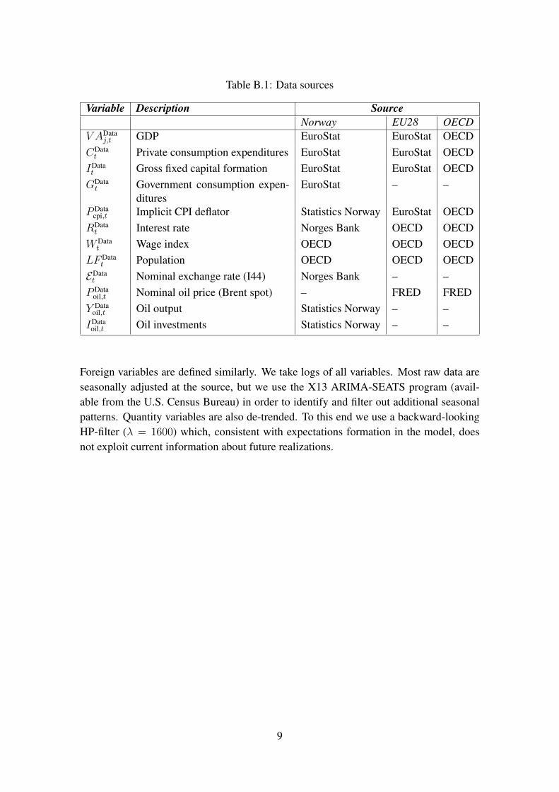
Table B.1: Data sources
Variable Description SourceNorway EU28 OECD
V ADataj,t GDP EuroStat EuroStat OECD
CDatat Private consumption expenditures EuroStat EuroStat OECD
IDatat Gross fixed capital formation EuroStat EuroStat OECDGDatat Government consumption expen-
dituresEuroStat – –
PDatacpi,t Implicit CPI deflator Statistics Norway EuroStat OECDRDatat Interest rate Norges Bank OECD OECD
WDatat Wage index OECD OECD OECD
LFDatat Population OECD OECD OECD
EDatat Nominal exchange rate (I44) Norges Bank – –PData
oil,t Nominal oil price (Brent spot) – FRED FREDY Data
oil,t Oil output Statistics Norway – –IData
oil,t Oil investments Statistics Norway – –
Foreign variables are defined similarly. We take logs of all variables. Most raw data areseasonally adjusted at the source, but we use the X13 ARIMA-SEATS program (avail-able from the U.S. Census Bureau) in order to identify and filter out additional seasonalpatterns. Quantity variables are also de-trended. To this end we use a backward-lookingHP-filter (λ = 1600) which, consistent with expectations formation in the model, doesnot exploit current information about future realizations.
9

C ROBUSTNESS ANALYSIS USING OECD DATA
The main analysis uses data from EU28 as proxy for the international economy. EU28accounts for 2/3 of Norway’s international trade, and harmonized data on sectoral valueadded are available for all EU28 members in addition to Norway. The main drawback ofthe EU data is that they cover less than a quarter of world GDP. This section, therefore,redo the analysis using OECD as proxy for the global economy. OECD data do notinclude sectoral variables, but they cover about 2/3 of global GDP. Details about the dataare reported in the data appendix.
C.1 VAR RESULTS
First, we re-estimate the VAR model in the paper. Impulse responses are shown in Fig-ure C.1 and Figure C.2, respectively. They are based on the same identification schemeas in the main paper. Qualitatively, we note similar responses as with EU28 data. Thatis, both the oil price shock and the international activity shock are associated with risingsectoral value added in all three sectors in Norway. The oil price shock is also associatedwith exchange rate appreciation. Quantitatively, we observe more persistent responses tothe oil price shock in the domestic economy when OECD data are used.
C.2 ESTIMATED DSGE PARAMETERS
Next, we estimate the DSGE model using OECD data. The model itself is left unchanged,as well as priors and the calibration. Prior and posterior parameters are reported in Ta-ble C.1. We emphasize a couple of observations: first, both the estimated oil demandelasticity and the volatility of international oil productivity shocks are higher than in themain analysis. Higher substitution elasticity implies smaller effects of oil price shocks inthe international economy (due to more substitution towards other goods). More volatileoil supply shocks imply the opposite. Second, most of the international shocks are lesspersistent when OECD data are used. This suggests that international shocks might playa smaller role for the domestic economy at long forecasting horizons, compared with theresults based on data from EU28. Most other parameters are fairly similar to those in themain text.
C.3 FILTERED PREDICTIONS
Figure C.3 compares OECD data with one step ahead predictions from the model. Thefit is largely comparable with that using EU data, although it deteriorates somewhat forpublic demand and the exchange rate. Measurement errors play, once again, only a minorrole.
10

C.4 FORECAST ERROR VARIANCE DECOMPOSITION
Figure C.4 reports the forecast error variance decomposition of mainland GDP. Comparedwith the baseline, we find that foreign shocks are more important in the short run. How-ever, both foreign macro shocks and the foreign oil supply shock are less dominant at longhorizons. At the 10 years horizon, the variance share accounted for by oil supply dropsfrom 33% to 19%. This number is still consistent with the view that oil price volatility isimportant for mainland GDP.
C.5 IMPULSE RESPONSES
Posterior impulse responses to an oil price shock are reported in Figure C.5 and Fig-ure C.6, respectively. They are largely comparable with those based on EU data. Quali-tatively, an oil price boom leads to lower activity abroad and higher activity in Norway.The shapes of the responses resemble closely those in the main analysis. Quantitatively,we see that most effects in OECD are slightly smaller, although the oil price dynamicsare largely unchanged. Also the Norwegian variables display somewhat smaller effects,consistent with the variance decomposition described above.
11

Figure C.1: International oil price shock
(a) Oil price (b) International output (c) Exchange rate
(d) Oil sector (e) Manufacturing (f) Services
Note: Impulse responses to a one standard deviation shock to the real oil price. Calculations are based on1000 draws from the posterior distribution. Median and 68 % credible bands.
Figure C.2: International activity shock
(a) Oil price (b) International output (c) Exchange rate
(d) Oil sector (e) Manufacturing (f) Services
Note: Impulse responses to a one standard deviation shock to international activity. Calculations are basedon 1000 draws from the posterior distribution. Median and 68 % credible bands.
12

Table C.1: Prior and posterior distributions
Prior Posterior domestic and oil Posterior foreign
Prior(P1,P2) Mode Mean 5%-95% Mode Mean 5%-95%
χC Habit B(0.70,0.10) 0.86 0.74 0.64-0.91 0.82 0.80 0.75-0.86εI Inv. adj. cost G(5.00,1.00) 5.83 6.18 5.20-7.16 4.96 5.23 4.43-6.00θw Calvo wages B(0.65,0.07) 0.80 0.75 0.68-0.81 0.84 0.83 0.79-0.87ιw Indexation, πw B(0.30,0.15) 0.42 0.48 0.31-0.63 0.37 0.42 0.28-0.56θpm Calvo manu. B(0.45,0.07) 0.55 0.57 0.51-0.62 0.57 0.53 0.47-0.58θps Calvo serv. B(0.65,0.07) 0.69 0.72 0.67-0.77 0.92 0.92 0.89-0.94ιp Indexation, πp B(0.30,0.15) 0.64 0.59 0.44-0.72 0.20 0.22 0.12-0.34ρr Smoothing, r B(0.50,0.10) 0.85 0.84 0.81-0.87 0.69 0.70 0.64-0.77ρπ Taylor, π N(2.00,0.20) 2.13 2.22 2.08-2.36 1.70 1.61 1.51-1.70ρde Taylor, ∆e N(0.10,0.05) 0.01 0.07 0.00-0.12 – – –ρy Taylor, gdp N(0.13,0.05) 0.13 0.17 0.11-0.23 0.12 0.10 0.05-0.15η H-F elasticity G(1.00,0.15) 0.62 0.63 0.57-0.69 – – –τy Fiscal, gdp N(0.00,0.15) 0.15 0.14 0.02-0.28 – – –τo Fiscal, swf N(0.00,0.15) 0.05 0.08 0.03-0.14 – – –ρg Fiscal, g B(0.50,0.15) 0.55 0.47 0.34-0.64 – – –εO Inv. adj. cost oil G(5.00,1.00) 6.00 5.69 4.65-6.55 – – –ς∗d Oil demand elast. G(0.30,0.15) – – – 0.55 0.53 0.43-0.64ς∗s Oil supply elast. G(0.30,0.15) – – – 0.01 0.01 0.00-0.02ρA Technology B(0.35,0.15) 0.37 0.42 0.31-0.55 0.71 0.74 0.66-0.83ρI Investment B(0.35,0.15) 0.43 0.32 0.17-0.47 0.47 0.50 0.41-0.59ρU Preferences B(0.35,0.15) 0.46 0.69 0.39-0.88 0.89 0.82 0.70-0.93ρW Wage markup B(0.35,0.15) 0.53 0.64 0.53-0.74 0.53 0.47 0.33-0.66ρM Price markup B(0.35,0.15) 0.87 0.88 0.83-0.94 0.74 0.71 0.65-0.78ρB UIP B(0.50,0.15) 0.95 0.94 0.92-0.96 – – –ρF Oil investment B(0.50,0.15) 0.71 0.80 0.70-0.89 – – –ρAo Oil supply B(0.50,0.15) 0.71 0.74 0.66-0.83 0.83 0.89 0.83-0.94σAm Sd tech. manu. IG(0.50,2.00) 1.22 1.26 1.01-1.49 0.52 0.53 0.33-0.72σAs Sd tech. serv. IG(0.50,2.00) 1.28 1.39 1.01-1.77 7.23 7.41 6.33-8.46σI Sd investment IG(0.50,2.00) 10.97 13.11 9.48-16.32 0.65 0.85 0.48-1.22σU Sd preferences IG(0.50,2.00) 5.97 4.22 2.32-7.61 1.14 1.12 0.77-1.47σG Sd government IG(0.50,2.00) 0.95 0.87 0.75-0.99 – – –σW Sd labor supply IG(0.10,2.00) 0.26 0.24 0.18-0.29 0.09 0.11 0.07-0.15σMm Sd markup manu. IG(0.10,2.00) 0.45 0.46 0.30-0.63 0.11 0.14 0.07-0.21σMs Sd markup serv. IG(0.10,2.00) 0.10 0.13 0.08-0.17 0.07 0.10 0.07-0.13σR Sd mon. pol. IG(0.02,2.00) 0.14 0.16 0.13-0.18 0.13 0.14 0.11-0.17σB Sd UIP IG(0.50,2.00) 0.24 0.25 0.20-0.29 – – –σF Sd oil inv. IG(0.50,2.00) 10.83 9.34 7.14-11.53 – – –σAo Sd oil supply IG(0.50,2.00) 2.69 2.89 2.50-3.26 7.24 6.31 4.53-8.07
Note: Posterior moments are computed from 5,000,000 draws generated by the Random Walk Metropolis-Hastings algo-rithm, where the first 4,000,000 are used as burn-in. B denotes the beta distribution, N normal, G gamma, and IG inversegamma. P1 and P2 denote the prior mean and standard deviation. For IG, P1 and P2 denote the prior mode and degreesof freedom, respectively. Shock volatilities are multiplied by 100 relative to the text.
13

Figu
reC
.3:D
ata
vers
uson
est
epah
ead
filte
red
estim
ates
(med
ian)
–O
EC
D
1995
2005
2015
−505
GD
P N
OR
WA
Y
1995
2005
2015
−10−505
VA
LUE
AD
DE
D M
. NO
RW
AY
1995
2005
2015
−4
−2024
VA
LUE
AD
DE
D S
. NO
RW
AY
1995
2005
2015
−4
−202
CO
NS
UM
PT
ION
NO
RW
AY
1995
2005
2015
−10010
INV
ES
TM
EN
T N
OR
WA
Y
1995
2005
2015
−202
PU
BLI
C D
EM
AN
D N
OR
WA
Y
1995
2005
2015
−202
WA
GE
INF
LAT
ION
NO
RW
AY
1995
2005
2015
−101
INF
LAT
ION
NO
RW
AY
1995
2005
2015
−0.
50
0.5
INT
ER
ES
T R
AT
E N
OR
WA
Y
1995
2005
2015
−10010
EX
CH
AN
GE
RA
TE
NO
RW
AY
1995
2005
2015
−10−505
OIL
OU
TP
UT
NO
RW
AY
1995
2005
2015
−20020
OIL
INV
ES
TM
EN
T N
OR
WA
Y
1995
2005
2015
−4
−202
GD
P O
EC
D
1995
2005
2015
−4
−202
CO
NS
UM
PT
ION
OE
CD
1995
2005
2015
−10−50
INV
ES
TM
EN
T O
EC
D
1995
2005
2015
−202
WA
GE
INF
LAT
ION
OE
CD
1995
2005
2015
−10123
INF
LAT
ION
OE
CD
1995
2005
2015
−0.
50
0.5
INT
ER
ES
T R
AT
E O
EC
D
1995
2005
2015
−50050100
BR
EN
T O
IL P
RIC
E
RA
W D
AT
AD
AT
A A
CC
OU
NT
ING
FO
R M
EA
SU
RE
ME
NT
ER
RO
RS
MO
DE
L
14

Figure C.4: Forecast error variance decomposition of mainland GDP
5 10 15 20 25 30 35 400
10
20
30
40
50
60
70
80
90
100
Horizon (quarters)
Var
ianc
e de
com
posi
tion
(%)
18.3%
21.2%
48.8%
11.3%0.4%
28.7%
17.4%
18.6%
16.5%
18.9%
0
10
20
30
40
50
60
70
80
90
100
Note: Forecast error variance decomposition of GDP in mainland Norway. Calculated at the posterior mean.Shocks are decomposed as follows: Domestic supply shocks (light blue), domestic demand shocks (darkblue), international supply shocks (light green), international demand shocks (dark green), and shocks inoil markets (light red). Numbers in white at the left and right hand side are decompositions at the 1- and40-quarter horizons, respectively.
Figure C.5: International responses to an international oil price shock – OECD data
5 10 15 20
−0.15
−0.1
−0.05
0
GDP
5 10 15 20
−0.1
−0.05
0
CONSUMPTION
5 10 15 20
−0.4
−0.3
−0.2
−0.1
0
INVESTMENT
5 10 15 20
−0.06
−0.04
−0.02
REAL WAGE
5 10 15 200
0.05
0.1
0.15
PRICE INFLATION
5 10 15 200
0.05
0.1
INTEREST RATE
5 10 15 20−0.2
−0.15
−0.1
−0.05
0
GDP MANUFACTURING
5 10 15 20
−0.15
−0.1
−0.05
0
GDP SERVICES
5 10 15 20
2468
101214
OIL PRICE
Note: Bayesian impulse responses of international variables to an international oil price shock (one standarddeviation). Mean (solid line) and 90% highest probability intervals (shaded area) based on every 1000thdraw from the posterior MCMC chain. Inflation and the interest rate are expressed in annual terms.
15

Figure C.6: Domestic responses to an international oil price shock – OECD data
5 10 15 20
0
0.1
0.2
0.3
GDP
5 10 15 20
0.2
0.4
0.6
CONSUMPTION
5 10 15 200.2
0.4
0.6
0.8
1
1.2
1.4INVESTMENT
5 10 15 20
−0.35
−0.3
−0.25
−0.2
TRADE BALANCE
5 10 15 20
0.1
0.2
0.3
0.4REAL WAGE
5 10 15 20
−0.15
−0.1
−0.05
0PRICE INFLATION
5 10 15 20
−0.1
−0.08
−0.06
−0.04
INTEREST RATE
5 10 15 20
−0.8
−0.7
−0.6
−0.5
−0.4
EXCHANGE RATE
5 10 15 20
−0.1
0
0.1
0.2
0.3
GDP MANUFACTURING
5 10 15 200
0.1
0.2
0.3
0.4
GDP SERVICES
5 10 15 200
5
10
GDP OIL
5 10 15 200
1
2
3
INVESTMENTS OIL
Note: Bayesian impulse responses of domestic variables to an international oil price shock (one standarddeviation). Mean (solid line) and 90% highest probability intervals (shaded area) based on every 1000thdraw from the posterior MCMC chain. All variables except value added and investments in oil are from themainland economy. Inflation and the interest rate are expressed in annual terms.
16

D ADDITIONAL FIGURES AND TABLES
Table D.1: Steady state ratios in the benchmark model
Description Data Model
C/VA Consumption share in aggregate GDP 0.38 0.39
I/VA Investment share in aggregate GDP 0.21 0.21
G/VA Public spending share in aggregate GDP 0.21 0.20
(A∗H +O)/VA Export share in aggregate GDP 0.48 0.48
AF/VA Import share in aggregate GDP 0.28 0.28
GDPo/VA Oil share in aggregate GDP 0.22 0.21
GDPm/VA Manufacturing share in aggregate GDP 0.29 0.33
GDPs/VA Service sector share in aggregate GDP 0.49 0.46
Io/I Oil share in aggregate investments 0.25 0.24
O/(A∗H +O) Oil share in aggregate exports 0.47 0.45
µm Share of labor force in manufacturing – 0.41
µs Share of labor force in services – 0.57
µo Share of labor force in oil sector – 0.02
Note: This table presents ratios in the non-stochastic steady state as implied by the baselinecalibration. Data refers to corresponding sample averages in the data.
17

Figu
reD
.1:S
moo
thed
shoc
ks(9
0%hi
ghes
tpro
babi
lity
dens
ities
)
1995
2005
2015
−2
−1012
εAm
1995
2005
2015
−202
εAs
1995
2005
2015
−202
εI
1995
2005
2015
−202
εU
1995
2005
2015
−202
εG
1995
2005
2015
−202
εW
1995
2005
2015
−2
−1012
εM
m
1995
2005
2015
−2
−101
εM
s
1995
2005
2015
−2
−1012
εR
1995
2005
2015
−202
εAo
1995
2005
2015
−202
εF
1995
2005
2015
−1012
ε∗ B
1995
2005
2015
−3
−2
−101
ε∗ Ao
1995
2005
2015
−1
−0.
50
0.51
ε∗ Am
1995
2005
2015
−1
−0.
50
0.51
ε∗ As
1995
2005
2015
−101
ε∗ I
1995
2005
2015
−2
−101
ε∗ U
1995
2005
2015
−101
ε∗ W
1995
2005
2015
−0.
6
−0.
4
−0.
20
0.2
0.4
ε∗ M
m
1995
2005
2015
−1
−0.
50
0.5
ε∗ M
s
1995
2005
2015
−101
ε∗ R
18
Figu
reD
.2:E
mpi
rica
l(bl
ack)
and
theo
retic
al(b
lue)
seco
ndm
omen
ts,d
omes
ticec
onom
y
01
23
45
−1
−0.
500.
51
gdpt−
j
gdpt
01
23
45
−1
−0.
500.
51
gdpm,t−j
01
23
45
−1
−0.
500.
51
gdps,t−j
01
23
45
−1
−0.
500.
51
ct−
j
01
23
45
−1
−0.
500.
51
i t−j
01
23
45
−1
−0.
500.
51
πw,t−j
01
23
45
−1
−0.
500.
51
πt−
j
01
23
45
−1
−0.
500.
51
rt−
j
01
23
45
−1
−0.
500.
51
∆et−
j
01
23
45
−1
−0.
500.
51
ot−
j
01
23
45
−1
−0.
500.
51i o,t−j
01
23
45
−1
−0.
500.
51
gdpm,t
01
23
45
−1
−0.
500.
51
01
23
45
−1
−0.
500.
51
01
23
45
−1
−0.
500.
51
01
23
45
−1
−0.
500.
51
01
23
45
−1
−0.
500.
51
01
23
45
−1
−0.
500.
51
01
23
45
−1
−0.
500.
51
01
23
45
−1
−0.
500.
51
01
23
45
−1
−0.
500.
51
01
23
45
−1
−0.
500.
51
01
23
45
−1
−0.
500.
51
gdps,t
01
23
45
−1
−0.
500.
51
01
23
45
−1
−0.
500.
51
01
23
45
−1
−0.
500.
51
01
23
45
−1
−0.
500.
51
01
23
45
−1
−0.
500.
51
01
23
45
−1
−0.
500.
51
01
23
45
−1
−0.
500.
51
01
23
45
−1
−0.
500.
51
01
23
45
−1
−0.
500.
51
01
23
45
−1
−0.
500.
51
01
23
45
−1
−0.
500.
51
ct
01
23
45
−1
−0.
500.
51
01
23
45
−1
−0.
500.
51
01
23
45
−1
−0.
500.
51
01
23
45
−1
−0.
500.
51
01
23
45
−1
−0.
500.
51
01
23
45
−1
−0.
500.
51
01
23
45
−1
−0.
500.
51
01
23
45
−1
−0.
500.
51
01
23
45
−1
−0.
500.
51
01
23
45
−1
−0.
500.
51
01
23
45
−1
−0.
500.
51
it
01
23
45
−1
−0.
500.
51
01
23
45
−1
−0.
500.
51
01
23
45
−1
−0.
500.
51
01
23
45
−1
−0.
500.
51
01
23
45
−1
−0.
500.
51
01
23
45
−1
−0.
500.
51
01
23
45
−1
−0.
500.
51
01
23
45
−1
−0.
500.
51
01
23
45
−1
−0.
500.
51
01
23
45
−1
−0.
500.
51
01
23
45
−1
−0.
500.
51
πw,t
01
23
45
−1
−0.
500.
51
01
23
45
−1
−0.
500.
51
01
23
45
−1
−0.
500.
51
01
23
45
−1
−0.
500.
51
01
23
45
−1
−0.
500.
51
01
23
45
−1
−0.
500.
51
01
23
45
−1
−0.
500.
51
01
23
45
−1
−0.
500.
51
01
23
45
−1
−0.
500.
51
01
23
45
−1
−0.
500.
51
01
23
45
−1
−0.
500.
51
πt
01
23
45
−1
−0.
500.
51
01
23
45
−1
−0.
500.
51
01
23
45
−1
−0.
500.
51
01
23
45
−1
−0.
500.
51
01
23
45
−1
−0.
500.
51
01
23
45
−1
−0.
500.
51
01
23
45
−1
−0.
500.
51
01
23
45
−1
−0.
500.
51
01
23
45
−1
−0.
500.
51
01
23
45
−1
−0.
500.
51
01
23
45
−1
−0.
500.
51
rt
01
23
45
−1
−0.
500.
51
01
23
45
−1
−0.
500.
51
01
23
45
−1
−0.
500.
51
01
23
45
−1
−0.
500.
51
01
23
45
−1
−0.
500.
51
01
23
45
−1
−0.
500.
51
01
23
45
−1
−0.
500.
51
01
23
45
−1
−0.
500.
51
01
23
45
−1
−0.
500.
51
01
23
45
−1
−0.
500.
51
01
23
45
−1
−0.
500.
51
∆et
01
23
45
−1
−0.
500.
51
01
23
45
−1
−0.
500.
51
01
23
45
−1
−0.
500.
51
01
23
45
−1
−0.
500.
51
01
23
45
−1
−0.
500.
51
01
23
45
−1
−0.
500.
51
01
23
45
−1
−0.
500.
51
01
23
45
−1
−0.
500.
51
01
23
45
−1
−0.
500.
51
01
23
45
−1
−0.
500.
51
01
23
45
−1
−0.
500.
51
ot
01
23
45
−1
−0.
500.
51
01
23
45
−1
−0.
500.
51
01
23
45
−1
−0.
500.
51
01
23
45
−1
−0.
500.
51
01
23
45
−1
−0.
500.
51
01
23
45
−1
−0.
500.
51
01
23
45
−1
−0.
500.
51
01
23
45
−1
−0.
500.
51
01
23
45
−1
−0.
500.
51
01
23
45
−1
−0.
500.
51
01
23
45
−1
−0.
500.
51
io,t
01
23
45
−1
−0.
500.
51
01
23
45
−1
−0.
500.
51
01
23
45
−1
−0.
500.
51
01
23
45
−1
−0.
500.
51
01
23
45
−1
−0.
500.
51
01
23
45
−1
−0.
500.
51
01
23
45
−1
−0.
500.
51
01
23
45
−1
−0.
500.
51
01
23
45
−1
−0.
500.
51
01
23
45
−1
−0.
500.
51
19

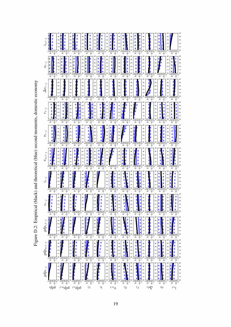
Figu
reD
.3:E
mpi
rica
l(bl
ack)
and
theo
retic
al(b
lue)
seco
ndm
omen
ts,d
omes
tican
dfo
reig
nec
onom
y
01
23
45
−1
−0.
500.
51
gdp∗ t−
j
gdpt
01
23
45
−1
−0.
500.
51
gdp∗ m,t−j
01
23
45
−1
−0.
500.
51
gdp∗ s,t−j
01
23
45
−1
−0.
500.
51
c∗ t−
j
01
23
45
−1
−0.
500.
51
i∗ t−j
01
23
45
−1
−0.
500.
51
π∗ w,t−j
01
23
45
−1
−0.
500.
51
π∗ t−
j
01
23
45
−1
−0.
500.
51
r∗ t−
j
01
23
45
−1
−0.
500.
51
p∗ ro,t−j
01
23
45
−1
−0.
500.
51
gdpm,t
01
23
45
−1
−0.
500.
51
01
23
45
−1
−0.
500.
51
01
23
45
−1
−0.
500.
51
01
23
45
−1
−0.
500.
51
01
23
45
−1
−0.
500.
51
01
23
45
−1
−0.
500.
51
01
23
45
−1
−0.
500.
51
01
23
45
−1
−0.
500.
51
01
23
45
−1
−0.
500.
51
gdps,t
01
23
45
−1
−0.
500.
51
01
23
45
−1
−0.
500.
51
01
23
45
−1
−0.
500.
51
01
23
45
−1
−0.
500.
51
01
23
45
−1
−0.
500.
51
01
23
45
−1
−0.
500.
51
01
23
45
−1
−0.
500.
51
01
23
45
−1
−0.
500.
51
01
23
45
−1
−0.
500.
51
ct
01
23
45
−1
−0.
500.
51
01
23
45
−1
−0.
500.
51
01
23
45
−1
−0.
500.
51
01
23
45
−1
−0.
500.
51
01
23
45
−1
−0.
500.
51
01
23
45
−1
−0.
500.
51
01
23
45
−1
−0.
500.
51
01
23
45
−1
−0.
500.
51
01
23
45
−1
−0.
500.
51
it
01
23
45
−1
−0.
500.
51
01
23
45
−1
−0.
500.
51
01
23
45
−1
−0.
500.
51
01
23
45
−1
−0.
500.
51
01
23
45
−1
−0.
500.
51
01
23
45
−1
−0.
500.
51
01
23
45
−1
−0.
500.
51
01
23
45
−1
−0.
500.
51
01
23
45
−1
−0.
500.
51
πw,t
01
23
45
−1
−0.
500.
51
01
23
45
−1
−0.
500.
51
01
23
45
−1
−0.
500.
51
01
23
45
−1
−0.
500.
51
01
23
45
−1
−0.
500.
51
01
23
45
−1
−0.
500.
51
01
23
45
−1
−0.
500.
51
01
23
45
−1
−0.
500.
51
01
23
45
−1
−0.
500.
51
πt
01
23
45
−1
−0.
500.
51
01
23
45
−1
−0.
500.
51
01
23
45
−1
−0.
500.
51
01
23
45
−1
−0.
500.
51
01
23
45
−1
−0.
500.
51
01
23
45
−1
−0.
500.
51
01
23
45
−1
−0.
500.
51
01
23
45
−1
−0.
500.
51
01
23
45
−1
−0.
500.
51
rt
01
23
45
−1
−0.
500.
51
01
23
45
−1
−0.
500.
51
01
23
45
−1
−0.
500.
51
01
23
45
−1
−0.
500.
51
01
23
45
−1
−0.
500.
51
01
23
45
−1
−0.
500.
51
01
23
45
−1
−0.
500.
51
01
23
45
−1
−0.
500.
51
01
23
45
−1
−0.
500.
51
∆et
01
23
45
−1
−0.
500.
51
01
23
45
−1
−0.
500.
51
01
23
45
−1
−0.
500.
51
01
23
45
−1
−0.
500.
51
01
23
45
−1
−0.
500.
51
01
23
45
−1
−0.
500.
51
01
23
45
−1
−0.
500.
51
01
23
45
−1
−0.
500.
51
01
23
45
−1
−0.
500.
51
ot
01
23
45
−1
−0.
500.
51
01
23
45
−1
−0.
500.
51
01
23
45
−1
−0.
500.
51
01
23
45
−1
−0.
500.
51
01
23
45
−1
−0.
500.
51
01
23
45
−1
−0.
500.
51
01
23
45
−1
−0.
500.
51
01
23
45
−1
−0.
500.
51
01
23
45
−1
−0.
500.
51
io,t
01
23
45
−1
−0.
500.
51
01
23
45
−1
−0.
500.
51
01
23
45
−1
−0.
500.
51
01
23
45
−1
−0.
500.
51
01
23
45
−1
−0.
500.
51
01
23
45
−1
−0.
500.
51
01
23
45
−1
−0.
500.
51
01
23
45
−1
−0.
500.
51
20

Figu
reD
.4:H
isto
rica
lvar
ianc
ede
com
posi
tion,
mai
nlan
dG
DP
1995
2005
2015
−505
εA,m
→gdp
1995
2005
2015
−505
εA,s→
gdp
1995
2005
2015
−505
εR→
gdp
1995
2005
2015
−505
εU→
gdp
1995
2005
2015
−505
εI→
gdp
1995
2005
2015
−505
εG→
gdp
1995
2005
2015
−505
εM
,m→
gdp
1995
2005
2015
−505
εM
,s→
gdp
1995
2005
2015
−505
εW
→gdp
1995
2005
2015
−505
ε∗ A,m
→gdp
1995
2005
2015
−505
ε∗ A,s→
gdp
1995
2005
2015
−505
ε∗ R→
gdp
1995
2005
2015
−505
ε∗ U→
gdp
1995
2005
2015
−505
ε∗ I→
gdp
1995
2005
2015
−505
ε∗ M
,m→
gdp
1995
2005
2015
−505
ε∗ M
,s→
gdp
1995
2005
2015
−505
ε∗ W
→gdp
1995
2005
2015
−505
ε∗ B→
gdp
1995
2005
2015
−505
ε∗ Ao→
gdp
1995
2005
2015
−505
εF→
gdp
1995
2005
2015
−505
εAo→
gdp
21

Figure D.5: Dynamics in domestic oil industry after an international oil price shock
20 40 60 80 1000
0.5
1
1.5
2
Yc
20 40 60 80 1000
1
2
3
Xc
20 40 60 80 100
0
1
2
Nc
20 40 60 80 100
0.20.40.60.8
11.2
Kc
20 40 60 80 1000
0.5
1
1.5
Io
20 40 60 80 1000
0.5
1
1.5
2
Qo
20 40 60 80 1000
0.5
1
P xr,c
20 40 60 80 100
0
1
2
3
Rkc
20 40 60 80 100
0.05
0.1
0.15
0.2
Yo
20 40 60 80 100
0.2
0.4
0.6
Fo
20 40 60 80 1000
0.2
0.4
0.6
Uo
20 40 60 80 100
0.2
0.4
0.6Fo
Note: Posterior mean impulse responses to an international oil price shock (one standard deviation). SeeFigure D.6 for details.
Figure D.6: An international oil price shock without the sovereign wealth fund
5 10 15 200
0.5
1
GDP
5 10 15 20
0
0.5
1
CONSUMPTION
5 10 15 200
0.5
1
1.5
2
INVESTMENT
5 10 15 20
−0.6
−0.4
−0.2
TRADE BALANCE
5 10 15 20
0.2
0.4
0.6REAL WAGE
5 10 15 20
−0.2
−0.1
0
0.1PRICE INFLATION
5 10 15 20
−0.1
0
0.1
INTEREST RATE
5 10 15 20
−0.8
−0.6
−0.4
−0.2
EXCHANGE RATE
5 10 15 20
0
0.5
1GDP MANUFACTURING
5 10 15 20
0.5
1
1.5
GDP SERVICES
5 10 15 200
5
10
GDP OIL
5 10 15 200
1
2
3
4
INVESTMENTS OIL
Note: Bayesian impulse responses to an international oil price shock (one standard deviation). Blue areasrepresent the baseline responses while gray dotted lines represent the counterfactual at the posterior mean.
22

Figure D.7: An international oil price shock without the supply chain
5 10 15 20
0
0.2
0.4
0.6
GDP
5 10 15 200
0.5
1
CONSUMPTION
5 10 15 200
0.5
1
1.5
2
INVESTMENT
5 10 15 20
−0.4
−0.3
−0.2
−0.1
0
TRADE BALANCE
5 10 15 200
0.2
0.4
0.6REAL WAGE
5 10 15 20
−0.2
−0.1
0
PRICE INFLATION
5 10 15 20
−0.15
−0.1
−0.05
0
INTEREST RATE
5 10 15 20
−0.8
−0.6
−0.4
−0.2
0
EXCHANGE RATE
5 10 15 20
0
0.2
0.4
0.6
GDP MANUFACTURING
5 10 15 20
0
0.2
0.4
0.6
0.8GDP SERVICES
5 10 15 200
5
10
GDP OIL
5 10 15 20
0
1
2
3
4
INVESTMENTS OIL
Note: Bayesian impulse responses to an international oil price shock (one standard deviation). Blue areasrepresent the baseline responses while gray dotted lines represent the counterfactual at the posterior mean.
Figure D.8: An international oil price shock without feedback to macro
5 10 15 20
0
0.2
0.4
0.6
GDP
5 10 15 20
0.2
0.4
0.6
0.8
1
CONSUMPTION
5 10 15 20
0.5
1
1.5
2
INVESTMENT
5 10 15 20
−0.4
−0.3
−0.2
−0.1
TRADE BALANCE
5 10 15 20
0.2
0.4
0.6REAL WAGE
5 10 15 20
−0.25
−0.2
−0.15
−0.1
−0.05
PRICE INFLATION
5 10 15 20
−0.15
−0.1
−0.05
INTEREST RATE
5 10 15 20
−0.8
−0.6
−0.4
−0.2
EXCHANGE RATE
5 10 15 20
0
0.2
0.4
0.6
GDP MANUFACTURING
5 10 15 20
0.2
0.4
0.6
0.8GDP SERVICES
5 10 15 200
5
10
GDP OIL
5 10 15 200
1
2
3
4
INVESTMENTS OIL
Note: Bayesian impulse responses to an international oil price shock (one standard deviation). Blue areasrepresent the baseline responses while gray dotted lines represent the counterfactual at the posterior mean.
23
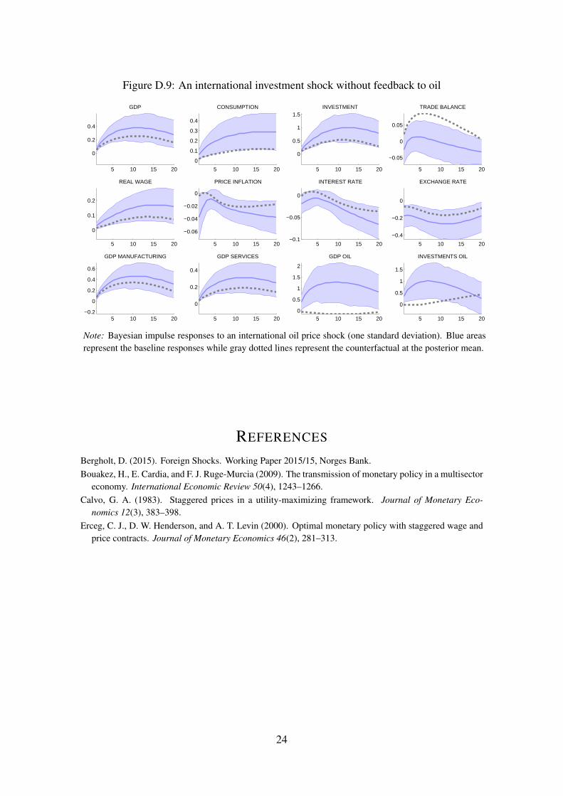
Figure D.9: An international investment shock without feedback to oil
5 10 15 20
0
0.2
0.4
GDP
5 10 15 20
0
0.1
0.2
0.3
0.4
CONSUMPTION
5 10 15 20
0
0.5
1
1.5INVESTMENT
5 10 15 20
−0.05
0
0.05
TRADE BALANCE
5 10 15 20
0
0.1
0.2
REAL WAGE
5 10 15 20
−0.06
−0.04
−0.02
0
PRICE INFLATION
5 10 15 20−0.1
−0.05
0
INTEREST RATE
5 10 15 20
−0.4
−0.2
0
EXCHANGE RATE
5 10 15 20−0.2
0
0.2
0.4
0.6
GDP MANUFACTURING
5 10 15 20
0
0.2
0.4
GDP SERVICES
5 10 15 200
0.5
1
1.5
2
GDP OIL
5 10 15 20
0
0.5
1
1.5
INVESTMENTS OIL
Note: Bayesian impulse responses to an international oil price shock (one standard deviation). Blue areasrepresent the baseline responses while gray dotted lines represent the counterfactual at the posterior mean.
REFERENCES
Bergholt, D. (2015). Foreign Shocks. Working Paper 2015/15, Norges Bank.Bouakez, H., E. Cardia, and F. J. Ruge-Murcia (2009). The transmission of monetary policy in a multisector
economy. International Economic Review 50(4), 1243–1266.Calvo, G. A. (1983). Staggered prices in a utility-maximizing framework. Journal of Monetary Eco-
nomics 12(3), 383–398.Erceg, C. J., D. W. Henderson, and A. T. Levin (2000). Optimal monetary policy with staggered wage and
price contracts. Journal of Monetary Economics 46(2), 281–313.
24