Business Efficiency - nationalparalegal.edunationalparalegal.edu/slides_new/Math/yk_9e/lesson3.pdf · Nearest Neighbor and Sorted Edges Algorithms Minimum-Cost Spanning Trees Kruskal’s

Chapter 2: Business Efficiency

Lesson Plan

Business Efficiency Visiting Vertices-Graph Theory Problem

Hamiltonian Circuits Vacation Planning Problem

Minimum Cost-Hamiltonian Circuit

Method of Trees

Fundamental Principle of Counting

Traveling Salesman Problem

Helping Traveling Salesmen Nearest Neighbor and Sorted Edges Algorithms

Minimum-Cost Spanning Trees

Kruskal’s Algorithm

Critical-Path Analysis

Mathematical Literacy in Today’s World, 9th ed.

For All Practical Purposes

© 2013 W. H. Freeman and Company


Business Efficiency

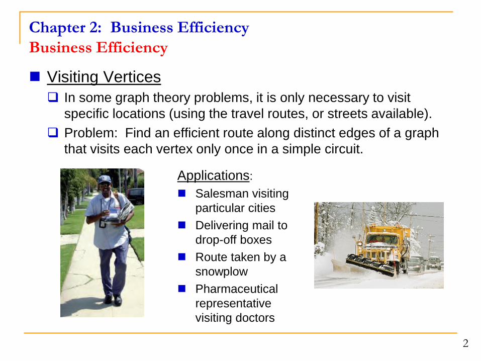
Visiting Vertices

In some graph theory problems, it is only necessary to visit

specific locations (using the travel routes, or streets available).

Problem: Find an efficient route along distinct edges of a graph

that visits each vertex only once in a simple circuit.

Applications:

Salesman visiting

particular cities

Delivering mail to

drop-off boxes

Route taken by a

snowplow

Pharmaceutical

representative

visiting doctors

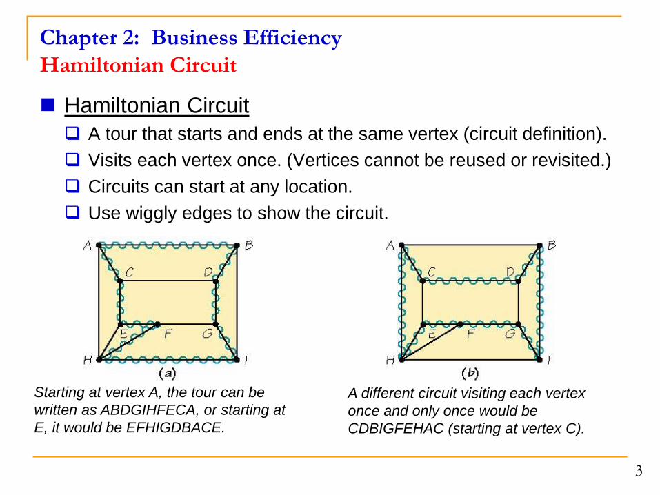
Hamiltonian Circuit

A tour that starts and ends at the same vertex (circuit definition).

Visits each vertex once. (Vertices cannot be reused or revisited.)

Circuits can start at any location.

Use wiggly edges to show the circuit.

Starting at vertex A, the tour can be

written as ABDGIHFECA, or starting at

E, it would be EFHIGDBACE.


Hamiltonian Circuit

A different circuit visiting each vertex

once and only once would be

CDBIGFEHAC (starting at vertex C).

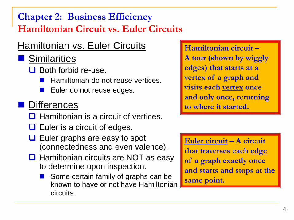
Hamiltonian vs. Euler Circuits

Similarities Both forbid re-use.

Hamiltonian do not reuse vertices.

Euler do not reuse edges.

Differences Hamiltonian is a circuit of vertices.

Euler is a circuit of edges.

Euler graphs are easy to spot (connectedness and even valence).

Hamiltonian circuits are NOT as easy to determine upon inspection.

Some certain family of graphs can be known to have or not have Hamiltonian

circuits.


Hamiltonian Circuit vs. Euler Circuits

Hamiltonian circuit –

A tour (shown by wiggly

edges) that starts at a

vertex of a graph and

visits each vertex once

and only once, returning

to where it started.

Euler circuit – A circuit

that traverses each edge

of a graph exactly once

and starts and stops at the

same point.


Hamiltonian Circuits

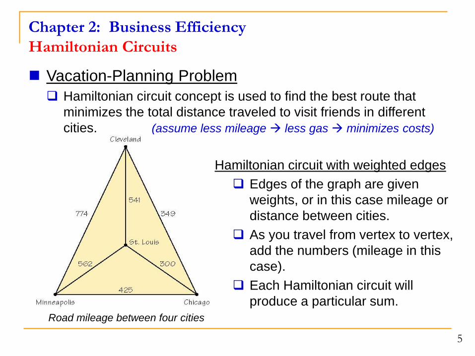
Vacation-Planning Problem

Hamiltonian circuit concept is used to find the best route that

minimizes the total distance traveled to visit friends in different

cities. (assume less mileage less gas minimizes costs)

Road mileage between four cities

Hamiltonian circuit with weighted edges

Edges of the graph are given

weights, or in this case mileage or

distance between cities.

As you travel from vertex to vertex,

add the numbers (mileage in this

case).

Each Hamiltonian circuit will

produce a particular sum.


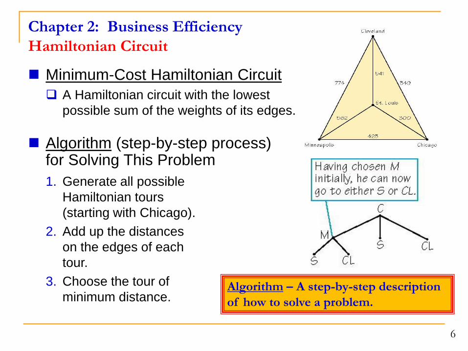
Hamiltonian Circuit

Algorithm – A step-by-step description

of how to solve a problem.

Minimum-Cost Hamiltonian Circuit

A Hamiltonian circuit with the lowest

possible sum of the weights of its edges.

Algorithm (step-by-step process) for Solving This Problem

1. Generate all possible

Hamiltonian tours

(starting with Chicago).

2. Add up the distances

on the edges of each

tour.

3. Choose the tour of

minimum distance.



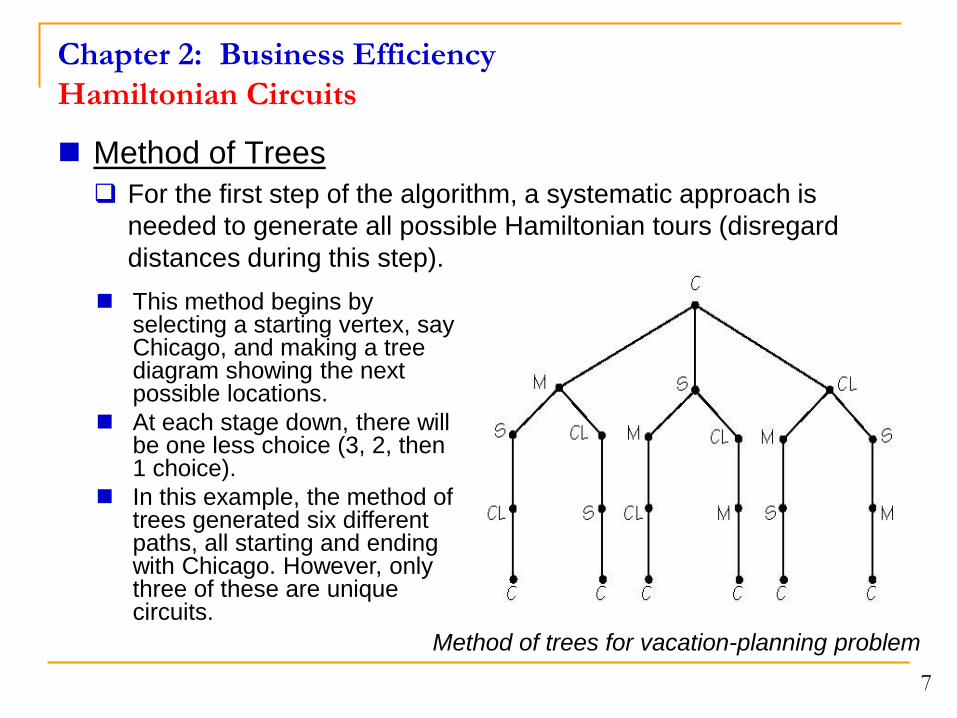
Method of trees for vacation-planning problem

Method of Trees

For the first step of the algorithm, a systematic approach is

needed to generate all possible Hamiltonian tours (disregard

distances during this step).

This method begins by selecting a starting vertex, say Chicago, and making a tree diagram showing the next possible locations.

At each stage down, there will be one less choice (3, 2, then 1 choice).

In this example, the method of trees generated six different paths, all starting and ending with Chicago. However, only three of these are unique circuits.



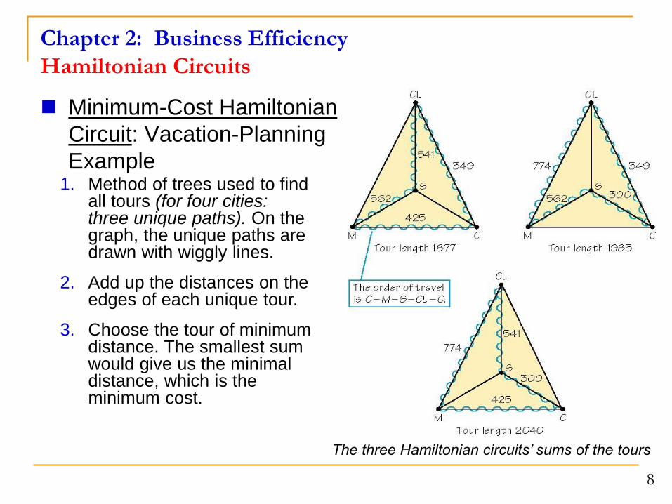
The three Hamiltonian circuits’ sums of the tours

Minimum-Cost Hamiltonian

Circuit: Vacation-Planning

Example 1. Method of trees used to find

all tours (for four cities: three unique paths). On the graph, the unique paths are drawn with wiggly lines.

2. Add up the distances on the edges of each unique tour.

3. Choose the tour of minimum distance. The smallest sum would give us the minimal distance, which is the minimum cost.


Hamiltonian Circuit

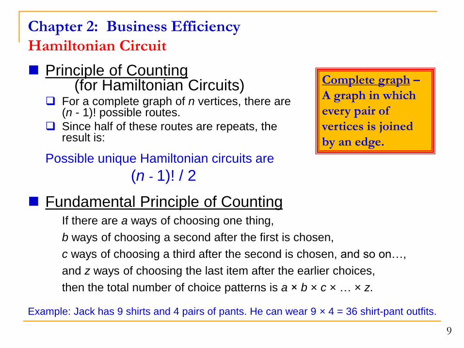
Principle of Counting (for Hamiltonian Circuits) For a complete graph of n vertices, there are

(n - 1)! possible routes.

Since half of these routes are repeats, the result is:

Possible unique Hamiltonian circuits are

(n - 1)! / 2

Complete graph –

A graph in which

every pair of

vertices is joined

by an edge.

Fundamental Principle of Counting If there are a ways of choosing one thing,

b ways of choosing a second after the first is chosen,

c ways of choosing a third after the second is chosen, and so on…,

and z ways of choosing the last item after the earlier choices,

then the total number of choice patterns is a × b × c × … × z.

Example: Jack has 9 shirts and 4 pairs of pants. He can wear 9 × 4 = 36 shirt-pant outfits.

Traveling Salesman Problem (TSP) Difficult to solve Hamiltonian circuits when the number of vertices

in a complete graph increases (n becomes very large).

This problem originated from a salesman determining his trip that minimizes costs (less mileage) as he visits the cities in a sales territory, starting and ending the trip in the same city.

There are many applications today: bus schedules, mail drop-offs, telephone booth coin pick-up routes, electric company meter readers, etc.

How can the TSP be solved? Computer programs can find the optimal route (not always

practical).

Heuristic methods can be used to find a “fast” answer, but does not guarantee that it is always the optimal answer.

Nearest neighbor algorithm

Sorted edges algorithm


Traveling Salesman Problem


Traveling Salesman Problem — Nearest Neighbor

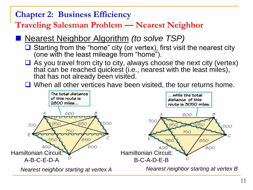
Nearest neighbor starting at vertex A

Nearest Neighbor Algorithm (to solve TSP) Starting from the “home” city (or vertex), first visit the nearest city

(one with the least mileage from “home”).

As you travel from city to city, always choose the next city (vertex) that can be reached quickest (i.e., nearest with the least miles), that has not already been visited.

When all other vertices have been visited, the tour returns home.

Nearest neighbor starting at vertex B

Hamiltonian Circuit:

A-B-C-E-D-A

Hamiltonian Circuit:

B-C-A-D-E-B


Traveling Salesman Problem — Sorted Edges

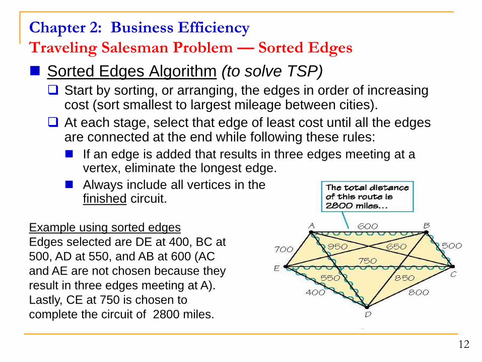
Sorted Edges Algorithm (to solve TSP) Start by sorting, or arranging, the edges in order of increasing

cost (sort smallest to largest mileage between cities).

At each stage, select that edge of least cost until all the edges are connected at the end while following these rules:

If an edge is added that results in three edges meeting at a vertex, eliminate the longest edge.

Always include all vertices in the finished circuit.

Example using sorted edges

Edges selected are DE at 400, BC at

500, AD at 550, and AB at 600 (AC

and AE are not chosen because they

result in three edges meeting at A).

Lastly, CE at 750 is chosen to

complete the circuit of 2800 miles.



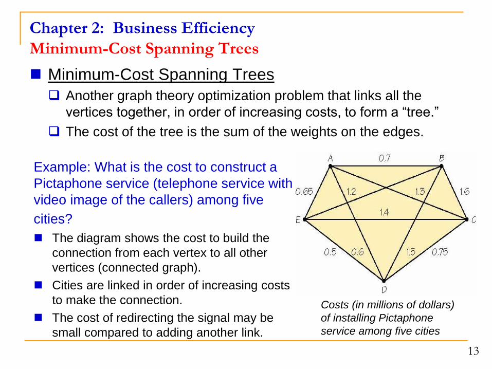
Costs (in millions of dollars)

of installing Pictaphone

service among five cities


Another graph theory optimization problem that links all the

vertices together, in order of increasing costs, to form a “tree.”

The cost of the tree is the sum of the weights on the edges.

Example: What is the cost to construct a

Pictaphone service (telephone service with

video image of the callers) among five

cities? The diagram shows the cost to build the

connection from each vertex to all other

vertices (connected graph).

Cities are linked in order of increasing costs

to make the connection.

The cost of redirecting the signal may be

small compared to adding another link.



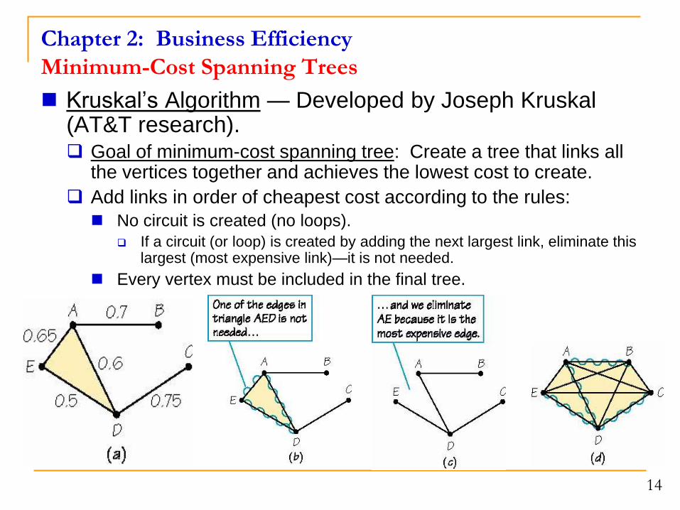
Kruskal’s Algorithm — Developed by Joseph Kruskal (AT&T research). Goal of minimum-cost spanning tree: Create a tree that links all

the vertices together and achieves the lowest cost to create.

Add links in order of cheapest cost according to the rules:

No circuit is created (no loops).

If a circuit (or loop) is created by adding the next largest link, eliminate this largest (most expensive link)—it is not needed.

Every vertex must be included in the final tree.


Critical Path Analysis

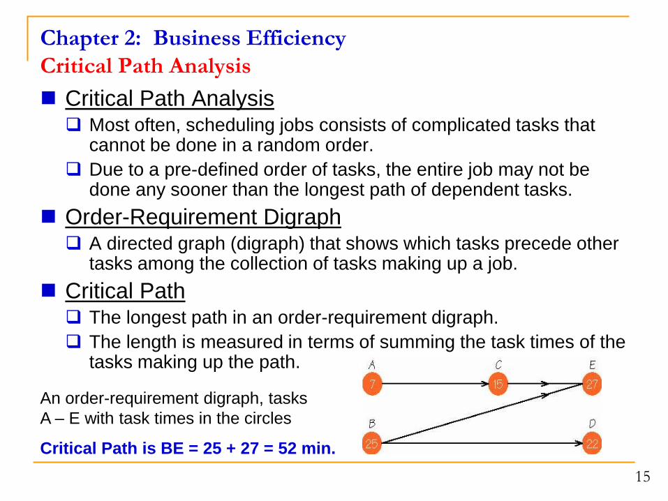
An order-requirement digraph, tasks

A – E with task times in the circles

Critical Path is BE = 25 + 27 = 52 min.

Critical Path Analysis Most often, scheduling jobs consists of complicated tasks that

cannot be done in a random order.

Due to a pre-defined order of tasks, the entire job may not be done any sooner than the longest path of dependent tasks.

Order-Requirement Digraph A directed graph (digraph) that shows which tasks precede other

tasks among the collection of tasks making up a job.

Critical Path The longest path in an order-requirement digraph.

The length is measured in terms of summing the task times of the tasks making up the path.

Documents

Business Efficiency - nationalparalegal.edunationalparalegal.edu/slides_new/Math/yk_9e/lesson3.pdf · Nearest Neighbor and Sorted Edges Algorithms Minimum-Cost Spanning Trees Kruskal’s