Embed Size (px)
Citation preview

NBER WORKING PAPER SERIES
BUSINESS IN A TIME OF SPANISH INFLUENZA
Howard Bodenhorn
Working Paper 27495http://www.nber.org/papers/w27495
NATIONAL BUREAU OF ECONOMIC RESEARCH1050 Massachusetts Avenue
Cambridge, MA 02138July 2020
I received no financial support for this research. The views expressed herein are those of the author and do not necessarily reflect the views of the National Bureau of Economic Research.
NBER working papers are circulated for discussion and comment purposes. They have not been peer-reviewed or been subject to the review by the NBER Board of Directors that accompanies official NBER publications.
© 2020 by Howard Bodenhorn. All rights reserved. Short sections of text, not to exceed two paragraphs, may be quoted without explicit permission provided that full credit, including © notice, is given to the source.

Business in a Time of Spanish InfluenzaHoward BodenhornNBER Working Paper No. 27495July 2020JEL No. N11
ABSTRACT
Mandated shutdowns of nonessential businesses during the COVID-19 crisis brought into sharp relief the tradeoff between public health and a healthy economy. This paper documents the short-run effects of shutdowns during the Spanish flu pandemic of 1918, which provides a useful counterpoint to choices made in 2020. The 1918 closures were shorter and less sweeping, in part because the US was at war and the Wilson administration was unwilling to let public safety jeopardize the war’s prosecution. The result was widespread sickness, which pushed some businesses to shutdown voluntarily; others operated shorthanded. Using hand-coded, high-frequency data (mostly weekly) this study reports three principal results. First, retail sales declined during the three waves of the pandemic; manufacturing activity slowed, but by less than retail. Second, worker absenteeism due to either sickness or fear of contracting the flu reduced output in several key sectors and industries that were not ordered closed by as much as 10 to 20% in weeks of high excess mortality. Output declines were the result of labor-supply rather than demand shocks. And, third, mandated closures are not associated with increases in the number or aggregate dollar value of business failures, but the number and aggregate dollar value of business failures increased modestly in weeks of high excess mortality. The results highlight that the tradeoff between mandated closures and economic activity is not the only relevant tradeoff facing public health authorities. Economic activity also declines, sometimes sharply, during periods of unusually high influenza-related illness and excess mortality even absent mandated business closures.
Howard BodenhornJohn E. Walker Department of EconomicsCollege of Business201-B Sirrine HallClemson UniversityClemson, SC 29634and [email protected]

1
“Business led me out sometimes to the other end of the town …
[and] it was a most surprising thing to see those streets, which were
usually thronged now grown desolate…I might sometimes have
gone the length of the whole street, I mean of the by-streets, and
seen nobody.” --Daniel Defoe, A Journal of the Plague Year
([1722]/1904, 19).
1. Introduction
One of the principal debates during the height of the COVID-19 crisis
in May 2020 concerned the tradeoff between the public health and economic
consequences of keeping non-essential businesses closed and people indoors.
Between February and April, after several weeks of lockdown and shelter-in-
place orders, the unemployment rate in the United States increased from a
near-historic low of 3.5% to 14.7%, or one not witnessed since the Great
Depression (BLS 2020). In April 2020 alone, nonfarm payrolls fell by 20.5
million – the leisure and hospitality (7.7 million) and retail (2.1 million) sectors
suffered the largest declines. Retail sales fell 16.4% and manufacturing output
declined 13.7%, each of which was the largest single monthly decline on record
(Torry 2020). In the first five months of 2020, more than 100,000 Americans
died from influenza-related complications (CDC 2020). The counterfactual is
hard to know, but in early January some epidemiological models predicted,
absent mandatory closings and social distancing measures, as many as 2.5
million excess deaths. Economists talk about tradeoffs. The decision to lock
down retail and manufacturing establishments in order to “flatten the curve”
was a tradeoff of enormous consequence.
In 1918 government officials at all levels also struggled with the
tradeoff between public health and a healthy economy. Woodrow Wilson’s
administration was concerned with a different tradeoff. It could wage total war

2
in Europe or it could quarantine army bases to stop the spread of the Spanish
flu. It chose to prosecute the war. The administration made the decision
knowing that either large numbers of young men would die of complications
from influenza in American military installations and on troop ships bound for
France, or more of them would die in trenches (Barry 2018). At the same time,
Philadelphia’s inept, corrupt, and much-maligned public health officials
delayed issuing quarantine orders and Philadelphians died at the highest rate
of any large US city. Wirth (2006, 322) recognizes, however, that the decisions
of the director of the city’s Department of Public Health, Dr. Wilmer Krusen,
were driven by his sense of balance between “public health with the city’s
desire for a robust economy.” Krusen’s choices now seem wrongheaded, but
in October 1918 the city’s leaders were under such intense pressure from
federal Liberty Loan administrators to meet the city’s sales quota and the war
department to keep the city’s shipyards open that his decision to lean toward
the robust economy may not have been as negligent as it appears in retrospect.
When the virus started to spread in autumn 1918, local public health
authorities responded with a number of traditional measures adopted during
previous polio and cholera epidemics: isolation of infected individuals,
quarantine of those having contact with infected individuals, surveillance of
at-risk populations (school students), disinfection and hygiene, targeted
closings, and public service announcements (Rosner 2010, 45). Municipal and
state public health officials closed schools, churches, theaters, restaurants, bars
and saloons; they shut down streetcars; they asked people to refrain from
nonessential travel of all kinds; they asked doctors who treated suspected cases
to report affected individuals and families to local officials; they limited
business hours. All of these measures took a toll on local businesses of all
kinds. Retail sales fell, sometimes precipitously (Garrett 2007). With public
transport shut down, employees’ commutes became more difficult. Worker
absenteeism increased. Manufacturing productivity declined.

3
People, of course, responded endogenously to the risk of venturing
out.1 Even those not afflicted refused to go out. In early October, prior to peak
mortality in Philadelphia, people were already avoiding each other; they were
isolating themselves. Barry (2018, 332) quotes one survivor: “We didn’t work.
Couldn’t go to work. Nobody came into work … they were all afraid.” Some
business owners did likewise. Grocers and dealers in all kinds of goods simply
closed up their stores, either because they were already ill or afraid that, if they
kept their stores open, they would become so. Thus, the virus created both
supply-side and demand-side effects. Worker absenteeism, whether among the
healthy or the sick, reduced production capabilities. As people refused to
venture out, sales of consumer goods declined. Sorting out the independent
supply- and demand-side effects is an empirical challenge.
This study assembles a wide variety of high-frequency qualitative and
quantitative data to shed light on the supply- and demand-side effects. Instead
of trying to identify the effects statistically through the use of exogenous
demand or supply shifters, the underlying hypothesis is that the federal
administration’s semi-nationalization of wartime production pushed much of
the US manufacturing sector to maintain operations in order to meet the
military’s needs. The production and sale of strictly civilian consumer goods
were not a federal priority. As a result, manufacturing and mining, especially
in war-related activities, were more likely to be affected by supply-side effects;
that is, declining manufacturing productivity and output were more likely to
be influenced by voluntary (fear) and involuntary (sickness) worker
absenteeism than from endogenous declines in demand. In the very short term,
however, civilian-oriented retail was more likely to be affected by endogenous
1 Economists have adapted standard epidemiological models of infectious disease spread to include behavioral responses to the risk of contracting the disease. A critical parameter in a standard SIRD (susceptible-infected-recovered-died) model of new infections, β, effectively accounts for the number of contacts an infected person has per day. Government mandates (shelter-in-place or closure orders) or individual decisions to self-isolate slow the rate of spread of the disease. A sufficiently large response will lead to the diseases dying out as the rate of new infections per infected person falls below one. Kermack and McKendrick (1927) develop the original SIR model as a system of differential equations; Fernandez-Villaverde and Jones (2020) provide a tractable extension that includes a time-varying β response parameter and a feedback effect that reduces the spread as people choose to avoid close contact with others.

4
demand shocks due to consumer illness or self-isolation than supply shocks
resulting from worker absenteeism.
Using hand-coded, high-frequency (mostly weekly) qualitative and
quantitative information, supplemented by narrative evidence, from a variety
of trade publications, this study documents the effects of the influenza
pandemic and mandated shutdowns, or nonpharmaceutical interventions, on
economic activity in several important economic sectors in the U.S. South. The
South is an informative case for several reasons: (1) the virus appeared early,
before officials were aware of its virulence and the salutary effects of mandated
closures; (2) the incidence of the flu varied across the region, from a maximum
weekly excess mortality rate of 200 per 100,000 population in Baltimore to 75
in Atlanta; (3) the South was home to several critical war-related industries,
including coal, cotton textiles, and lumber; and (4) the region’s business sector
was particularly hard hit by the virus, in that between 1915 and 1920 more
businesses failed in the South than in any other region and the failure rate on
a per capita basis exceeded the country’s other regions.2
The first set of results point to declines in both retail and
manufacturing activity in the weeks of unusually high influenza related deaths
that are attributable to both mandated closings and the sickness itself. The
independent effect of the influenza epidemic is evident during the two non-
peak waves of mortality that occurred after closing orders were lifted. Second,
quantitative evidence from the coal mining industry reveal almost pure supply-
side effects due to workers incapacitated by the disease through illness or a
reluctance to report to work for fear of catching it. Production in the South’s
principal coal fields in Kentucky and West Virginia declined by upwards of
15% at the height of the epidemic despite pressure from the US Fuel
Administration and War Department to meet the industry’s government-
established weekly output quotas. Third, narrative evidence from the region’s
textile- and lumber-producing regions points to equally large short-term
2 It is impossible at the moment to construct regional business failure rates because the principal sources of business failures did not provide estimates of the total number of businesses at risk at the regional level. See the discussion in Section 6 for further details concerning business failures.

5
declines of output. Declines in textile output are, like coal, almost purely labor-
supply driven, as the army needed uniforms and tent canvas. Declines in
lumber output, however, were due to a host of supply and demand-driven
factors. Finally, weekly reports of the number of business failures in the South
and elsewhere provide evidence that a rise in influenza-related mortality during
the pandemic was associated with an increased number of business failures.
The implementation of nonpharmaceutical interventions, as well as the
Armistice and immediate peace-time adjustments are, however, associated
with modest declines in the number of failures.
The evidence brings into sharp relief one feature of the tradeoff
between public health and a healthy economy. The COVID-19 debate focuses
on the economic costs of mandatory lockdowns and shelter-in-place orders.
Less discussion has focused on the economic costs of the counterfactual of
not locking down and not sheltering. History offers an object lesson. Any
comparison between 1918 and 2020 must be drawn carefully given advances
in medical practice, changes in the structure of the economy, and the inherent
differences between countries at war and peace. But wartime demands
militated against mandatory lockdowns and sheltering orders. One
consequence was that the Spanish flu virus was passed among workers and
several industries experienced epidemic outbreaks in their workplaces.
Productivity declined. Some of the South’s principal industries witnessed 25 to
50% worker absenteeism rates that reduced output by 10 to 20% for periods
between one and four weeks. Had it not been for federal administrators
pressuring these industries to maintain production in support of the war effort,
it is likely that the output declines would have been even larger. America’s
experience with the Spanish flu shows that any debate about health benefits
and economic costs of lockdowns and shelter-in-place orders must be
compared to a reasonable counterfactual in which more people die and the
economy still contracts. In short, the question is: how do we compare a 15%
unemployment rate and 100,000 deaths at the end of May 2020 to a “full-
employment” economy with a 7% sickness-induced absenteeism rate and,

6
perhaps, several multiples of the number of recorded deaths? The American
experience with the Spanish flu offers insights not answers.
2. The pandemic in the South
In late January 1918, Loring Miner, a country doctor in Haskell
County, Kansas, was called to treat several patients with what appeared to be
an unusual strain of seasonal influenza. The symptoms included a violent
headache and body aches, high fever, and a nonproductive cough, but he had
never before witnessed a flu that struck with such intensity. Its progress
through the body was rapid, and it killed, usually in short order. Within a
couple weeks, Miner lost dozens of patients. What was most distressing was
that those dying were the strongest, the heathiest, and the most robust young
men among those who came down with the flu. He contacted the U.S. Public
Health Service, but they offered him neither advice nor assistance (Barry 2018,
91-94).
At about the time Miner was confronted with an apparently new strain
of the influenza virus, several young men from Haskell County reported for
army basic training at Camp Funston in eastern Kansas. The weather that
winter was unusually cold and the quickly-constructed base did not provide
adequate shelter, heat, or outerwear. To keep the fresh recruits warm, as many
beds as possible were placed in each of the barracks and men huddled around
stoves. The first report of a flu-like sickness was reported on March 4. Within
weeks 1,100 men were admitted to the base hospital and thousands more were
treated in the infirmaries. Eventually, 237 men contracted pneumonia; 38 died.
Wartime exigencies and the need for men meant that Camp Funston supplied
a stream of potentially exposed or infected soldiers to the front lines in Europe,
where a particularly virulent and deadly strain of the influenza broke out,
spread, and was carried back to the US beginning in late summer 1918.
No one is sure whether the ‘Spanish flu’ originated in western Kansas
– some epidemiologists contend that it originated in China, Vietnam, or even
in the trenches in France – but at least one Nobel laureate who spent his life
studying influenza was convinced of its Kansas origins (Barry 2018, 98). When

7
it came back to the US, by way of troops returning from Europe through
Boston, it spread rapidly and killed at unprecedented rates. By mid-October
1918, when the typical influenza-pneumonia mortality rate would normally
have been about 2 per 100,000 per week, it rose above 94 in the 35 largest US
cities.3 Mortality rates remained above 10 through February 1919, or about
twice the median weekly mortality rate (Collins et al 1930, 2281 [Table 3]). A
second wave appeared in February 1920 when mortality rates briefly rose
above 28.
Figure 1 presents excess mortality rates in four representative southern
cities reported in Collins et al (1930), which mirror the experiences of other
major metropolitan areas, though there is substantial variation across cities.
Among southern cities, Baltimore experienced the highest excess mortality
rates, with a weekly peak of nearly 200 per 100,000 population. Southern cities
also reveal a range of experiences that accords with Collins et al’s (1930, 2301)
assertion that, while most people think of the pandemic as a singular, shared
event occurring in October and November 1918, the epidemic persisted, by
their accounting, for 31 weeks with a peak mortality on 19 October 1918.
Unusually high excess mortality rates continued, however, into March 1919.
While many cities experienced a second (some label it a third) peak in winter
1920, which on its own would qualify as an epidemic, it is dwarfed by the 1918
peak.
3 Epidemiological studies of the era combine influenza and pneumonia deaths because it was common for physicians to report influenza-related deaths as pneumonia.

8
Figure 1 Weekly excess mortality in four southern cities
Source: Collins et al (1930)
Southern officials responded to the appearance of the virus in much
the same way elected officials and health authorities elsewhere. Despite
published reports from Boston and New York about the seriousness of the
virus, when the first cases were reported in Wilmington, North Carolina, on
19 September 2018 the city’s public health commissioner assured residents that
it was probably a common flu and there was no call for unusual measures or
precautions (Cockrell 1996).4 Within a week, the city’s hospitals were
inundated with sick and dying patients. The virus radiated out from the port
city along the railroad lines. Within weeks, Kannapolis, a cotton mill town that
was home of Cannon Mills, located 30 miles north of Charlotte and with a
population of about 6,500 was thought to have had 2,000 cases of the flu.
Kannapolis’s three doctors, exhausted from overwork, begged for assistance.
Similar stories appear across the South. At Mississippi A&M College (now
4 Arkansas’ United States Public Health Service officer, James C. Geiger, is similarly quoted as having observed, on September 7, even after receiving reports of its virulence in Boston, that the obviously novel strain of the virus was a “simple, plain old-fashioned la grippe.” (Scott 1988, 320).
0
50
100
150
200
0
50
100
150
200
01jul
1916
01jul
1917
01jul
1918
01jul
1919
01jul
1920
01jul
1916
01jul
1917
01jul
1918
01jul
1919
01jul
1920
Baltimore Louisville
Memphis New Orleans
exce
ss m
orta
lity
per 1
0000
0
DateGraphs by cityno
Excess mortality in four southern cities

9
Mississippi State University) in Starkville, nearly all 1,800 students were
inducted into the army. More than half contracted the virus. By the time 36
died, the region’s US public health official noted that locals were near panic
(Barry 2018, 342-345).
Once southern municipal health authorities appreciated the
seriousness of the flu, they responded with a variety of measures aimed at
limiting the spread and mortality of the virus. Epidemiologists label them
nonpharmaceutical interventions (NPIs), which, when faced with a virus
without treatments or vaccines, are considered the most effective public health
responses. Schools, churches, dance halls, pool halls, saloons, and theatres
were closed. Retail store hours were shortened, usually to daylight hours to
limit after-work crowding when people shopped as they made their way home
(Woolley 1963). Even public funerals were suspended so that only immediate
family could mourn and still keep their distance from others.
< table 1 about here >
Table 1 reports the date of the first reported appearance of an
influenza case in select southern cities, the date the first NPI closure order was
issued, and the number of days any NPI was in effect. Markel et al (2007 and
supplementary online materials) report that although school and business
closure orders may have been issued on different dates, the orders were
sufficiently close in time that they cannot be studied separately using standard
statistical methods. That is, there were sometimes only a day or two between
an order to close schools and one to close certain businesses, so that it is
impossible to discern the independent effects of each with weekly or monthly
mortality data. There was about a two-week lag between the first reported
influenza case and the issuance of a closure order. The average length of

10
southern cities’ NPIs was 52 days. Louisville’s lockdown was the longest
among the city’s reported here; Memphis’s was likely the shortest.5
There is a general consensus in the epidemiological literature that
earlier and more comprehensive shutdown orders delayed peak mortality and
reduced peak and overall mortality, though the effects of non-pharmaceutical
interventions on overall mortality are smaller. Hatchett et al (2007) find that
cities with earlier and more interventions experienced peak mortality
approximately 50% lower than cities that did not intervene, but cumulative
excess mortality was reduced by about 20%. Bootsma and Ferguson (2007)
run simulations using a standard epidemiological transmission model and find
that short-term interventions, like those implemented in 1918, reduced total
mortality by 10 to 30%, but cities with longer more comprehensive NPIs
witnessed transmission rates 30 to 50% lower than other cities. Markel et al
(2007) and Barro (2020) use a larger sample of cities and find that cities with
earlier and broader bans on public gatherings experienced delayed peak
mortality, lower peak mortality rates, and lower total mortality. These studies
demonstrate a strong correlation between early and comprehensive closings.
They do not, however, address the potential tradeoff between economic losses
due to closings and the losses attributable to reduced economic activity
incidental to increased morbidity and mortality during a pandemic.
3. Economic consequences of the pandemic
Relying on narrative and anecdotal accounts, a number of histories of
the pandemic discuss its economic consequences at the macroeconomic and
the microeconomic levels. At the macro level is an account of Philadelphia’s
experience, which cites a contemporary Pennsylvania State Health
Commission report that estimated Philadelphia’s economic losses from the
pandemic in October 1918 alone to be $55 million, or about $27.50 per capita
5 Finger (2006) does not report the exact date of Memphis’ shutdown. He reports that by October 12, the city’s schools had been closed for a few days. I imputed Thursday, October 10 as the shutdown date, but it may have happened as early as Monday, October 7.

11
(Wirth 2006, 335).6 Although Philadelphia’s pandemic mortality experience
was worse than that experienced in any southern city, mortality rates were of
the same order of magnitude in Baltimore and New Orleans. Slosson (1930,
45) estimates that the total economic cost to the US of the 1918/19 pandemic
was $3 billion, or about 3.9% of gross domestic product (cited in McLaurin
1982).
At a less disaggregated level, a history of the epidemic in Paducah,
Kentucky finds that a local clothing manufacturer was forced to close for 10
days due to the high absenteeism rate among sick employees; a local newspaper
stopped publishing for more than a week for the same reason (Maupin 1975).
Local coal mines, too, suspended operations when worker absenteeism rose,
but the dollar value of any losses are not reported or estimated.
Whereas some businesses closed voluntarily as an endogenous
response to the outbreak, others were ordered closed by various municipal,
county, or state authorities. In the second week of October, North Carolina’s
state health commissioner imposed a ban on almost all social interactions that,
if strictly interpreted, would have closed nearly every business in the state. The
commissioner found it difficult to enforce his order, especially against small
businesses. When the board tried to enforce it against larger businesses, they
pushed back. Several large tobacco manufacturers appealed the closings to the
governor, but the governor refused to overturn the health officials’ orders.
Henry Pope, the federal Food and Drug Administration’s North Carolina
representative also protested the closing of a cottonseed oil mill because oil
was vital war materiel. Not every business resisted. When Shreveport’s health
authorities restricted business hours the president of the city’s Retail
Merchants’ Association asked businesses to comply. “The loss of a few
dollars,” he said, “is as nothing compared to the health of the people”
(McLaurin 1982, 7).
6 Wirth (2006) cites a newspaper clipping found in an archive as the source (Philadelphia Evening Bulletin, 31 October 1918), but I have not been able to locate any such report among the online records of the Pennsylvania Health Commission. The $27.50 estimate is equivalent to between $500 and $1,000 in constant 2020 dollars, depending on the conversion factor included at the Measuring Worth website (Williamson 2020).

12
Despite the reluctance of many businesses to shutter their doors,
Cockrell (1996, 314) writes that among those enterprises not forced to close
due to worker absenteeism, “many enterprises shut their doors voluntarily” for
a few weeks, at least, in response to the perceived danger. Following an
outbreak at a nearby military cantonment in early October, Shreveport
Louisiana’s theaters closed voluntarily rather than risk contributing to the
virus’s spread (McLaurin 1982). A study of Little Rock, Arkansas’ documents
the city’s quarantine order that closed schools, churches, and theaters, and
restricted retailers’ hours of operation, features Little Rock shared with other
cities. But the city’s health officials went farther when they prohibited
“bargain” sales to discourage crowds (Scott 1988, 331). While this last
restriction appears trifling at first blush, any late fall retail restriction threatened
the Christmas sales season, which was as important to some retailers then as
now.7
The COVID-19 outbreak has encouraged economists and economic
historians to document the consequences of epidemics and public health
responses to them. At a theoretical level, Eichenbaum et al (2020) extend a
standard epidemiological model of contagious disease to include the
interaction between economic choices and epidemic. Their results suggest that
people’s choices to reduce consumption and work to avoid contracting the
virus reduces the severity of the epidemic. It also necessarily reduces economic
activity by a nontrivial amount.
An early effort by an economist to document the costs of the pandemic
adds some quantitative analysis to the newspaper reports relied on by
historians. Garrett (2007) uses hand-collected reports from Little Rock and
Memphis and finds that retail businesses experienced substantial reductions in
sales during the pandemic. Smaller retailers in Little Rock reported sales
declines of 40 to 70 percent, and a department store reported a 50 percent
7 Dun’s Reports, which surveyed local business conditions in the pandemic era, repeatedly discussed holiday sales, especially at large department stores, as an indicator of the retail sector’s health. On 7 December 1918, for example, Dun’s published the following concerning Philadelphia’s retail sector: “With very great improvement in public health conditions, retail trade has assumed seasonable activity, the larger stores are crowded with holiday shoppers.”

13
decline. On October 19, near the epidemic’s peak, the reporter estimated that
Little Rock’s businesses were losing about $10,000 per day ($170,000 in 2019
dollars, or $2.60 per capita), mostly in spoilage of unsold goods, that would
not be realized when the quarantine was lifted. In Memphis, the city transit
authority reported that than 25 percent of their workers were out sick, and the
local phone company asked the public not to make unnecessary calls because
most of its operators were out sick.8
Most economic studies of the pandemic focus on its medium- to long-
term consequences. Brainerd and Siegler (2003) find a positive correlation
between states with high influenza mortality in 1918 and income growth over
the subsequent decade, which is consistent with the predictions of a standard
growth model in which the labor-capital ratio declines sharply. Barro et al
(2020) estimates suggest that US gross domestic product declined by 6% and
per capita consumption by 8%, which makes the pandemic the fourth costliest
event of the twentieth century behind the two world wars and the Great
Depression. Using a difference-in-differences approach Correia et al (2020)
find that the epidemic led to an average decrease in state-level manufacturing
output of 18% and an increase in bank loan charge-offs through 1923. They
also report that the adoption of more aggressive closings and social distancing
measures had a modest positive effect on economic activity in the years after
the epidemic. Lilley et al (2020), however, argue that once they control for
pre-existing trends the effect of non-pharmaceutical interventions studied by
Correia et al (2020) is “a noisy zero.” Finally, Almond (2006) finds that men
and women observed in 1960, 1970 and 1980 who were exposed to the virus
in utero exhibit lesser later-life attainments. They were 15% less likely to
graduate from high school, men’s wages were 5 to 9% lower, occupational
8 Back-of-the-envelope extrapolations from modern studies, assuming a 33% incidence rate for the Spanish flu rather than an average of 2.5% of a typical flu season, suggest per capita losses from lost work days during the pandemic between $6.75 and $13.10 in 1918, or about 0.9% to 1.8% of gross domestic product, which are of the same order of magnitude as contemporary estimates of retail sales losses (Akazawa et al 2003). The calculation does not account for changes in composition of the workforce over the twentieth century. Other studies suggest smaller losses in typical influenza years. See Thanner, et al (2011).

14
statuses were lower, poverty rates were higher, and they were more likely to
receive public support.
An exception of economists’ focus on medium- to long-term
consequences of the epidemic is Velde (2020). He looks at a number of
economic indicators at the monthly and, occasionally, weekly data in the
months surrounding the pandemic. Using standard time-series methodologies
(i.e., vector autoregressions) Velde finds that the epidemic and public health
interventions had small negative to zero effects on monthly retail sales,
employment, pig-iron production, and bank loans. Velde’s conclusion accords
with Arthur Burns and Wesley Claire Mitchell’s (1946) assessment that the
epidemic led to a modest, brief recession.
In a non-US context, Jordá et al (2020) find that major pandemics’
effects on real asset returns persist for as much as 40 years. Karlsson et al
(2014) uncover no discernible effects on earnings, but find that returns to
capital were reduced, and that poorhouse admissions increased in Sweden.
Percoco (2016) finds that in utero exposure to the virus among Italians reduced
later-life educational attainment. Guinmeau et al (2019) report negative effects
of exposure to the influenza on long-term health and labor productivity in São
Paulo, Brazil. Blickle (2020) finds that German regions experiencing higher
mortality rates had lower school spending and were more likely to vote for the
Nazis between 1925 and 1933.
Thus, existing research into the consequences of the pandemic reveal
a host of negative medium- and long-term consequences. This paper is closest
in spirit to Garrett’s (2007) in that it assesses the immediate impacts of the
virus and lockdowns on economic activity and Velde (2020) in the use of high-
frequency data. As Velde notes, the epidemic and NPIs were sufficiently short
that any assessment of its immediate and short-run impact requires high-
frequency (weekly or monthly) data. Although I make use of contemporary
narrative evidence, I also use high-frequency data on business activity, NPIs,
and excess mortality to investigate their supply-side and demand-side effects.
4. Data

15
The principal data on business conditions used here is hand-coded
from the source materials, mostly Bradstreet’s and Dun’s Review. Information on
city-level mortality was compiled by the public health service in the 1930s, and
information on business closings and quarantines comes from Bootsma and
Ferguson (2007) and Markel et al (2007).
4.1 Excess mortality
Collins et al (1930) reconstruct excess mortality for 35 large US cities
for which there is a continuous series of weekly mortality from influenza and
pneumonia from the onset of the pandemic in 1918. These two causes of death
are combined because most influenza victims die from pneumonia or
pneumonia-like complications that develop in consequence of the immune
system’s response to the viral infection. Prior to the pandemic, they report
monthly estimates of excess mortality calculated from data reported in
municipal and state health reports, as well as the US Census Bureau’s annual
Mortality Statistics.
The calculated excess mortality for the 31-week pandemic period are
relative to estimated median weekly death dates between 1910 and 1916, where
weekly rates prior to 1918 are inferred from plots of monthly data. Calculated
weekly excess mortality rates for the post-pandemic period are relative to
median rates between 1921 and 1927. To further smooth the median relatives,
Collins et al (1930) calculate excess mortality rates relative to the five-week
moving median weekly death rate. Thus, their excess mortality estimates are
calculated for city j in week t as:
𝐸𝐸𝐸𝐸𝐸𝐸𝐸𝐸𝐸𝐸𝐸𝐸 𝑚𝑚𝑚𝑚𝑚𝑚𝑚𝑚𝑚𝑚𝑚𝑚𝑚𝑚𝑚𝑚𝑚𝑚𝑗𝑗𝑗𝑗
= 𝑚𝑚𝑚𝑚𝑚𝑚𝑚𝑚𝑚𝑚𝑚𝑚𝑚𝑚𝑚𝑚𝑚𝑚𝑗𝑗𝑗𝑗
− � �15�
𝑗𝑗𝑗𝑗+2
𝑗𝑗𝑗𝑗−2𝑚𝑚𝐸𝐸𝑚𝑚𝑚𝑚𝑚𝑚𝑚𝑚 𝑚𝑚𝑚𝑚𝑚𝑚𝑚𝑚𝑚𝑚𝑚𝑚𝑚𝑚𝑚𝑚𝑚𝑚𝑗𝑗𝑗𝑗∈1910−16
The rates calculated in this way are the mortality data used in the analysis of
weekly data hereafter. Prior to September 1918, weekly rates are interpolated

16
from the city-level monthly rates reported in Collins et al (1930) using the
ipolate command in Stata.
4.2 Non-pharmaceutical interventions
Dates for which cities closed schools, churches, public transportation,
entertainment venues, and restricted the operating hours of some retail
businesses come primarily from Markel et al (2007) and Bootsma and
Ferguson (2007) and their online appendices. Table 1 lists the NPIs for the
seven large southern cities included in subsequent analyses (Atlanta, Baltimore,
Louisville, Memphis, Nashville, New Orleans, and Richmond), as well as for a
handful of smaller cities.
The first reports of influenza appeared in the second or third weeks of
September. Given that the onset of the epidemic is dated to the first week of
September in Boston, the virus appeared in southern cities in short order. Most
of the NPI orders were issued two to three weeks after the first influenza cases
were reported and most were rescinded in whole or in part by the last week of
October or first week in November.
The decision to allow public gatherings in early November probably
led to the second peak that appeared in most cities between late November
1918 and January 1919. When the Armistice was announced on 11 November,
for example, spontaneous public celebrations broke out in cities and towns
across the United States. People poured into the streets to celebrate, but this
kind of mingling was what the public health authorities had been trying to
avoid when they closed schools, churches, public transportation, and some
businesses. Health officers in Paducah, Kentucky and Little Rock, Arkansas,
in fact, attributed the late-November resurgence in reported cases and deaths
to the Armistice-day celebrations (Maupin 1975, Scott 1988). By the end of
November, conditions had deteriorated sufficiently in Arkansas that the state
health commissioners contemplated a second statewide shutdown.
The resurgence of the virus in late 1918 and early 1919 and its
reappearance in January and February 1920 did not elicit similar public health
responses affords the opportunity to estimate an endogenous public response

17
to the virus and disentangle its effects from the NPIs imposed during the peak
mortality weeks in October and November 1918. Relying exclusively on the
peak mortality period which coincided with closings and quarantines would
make separating their independent effect difficult. The second wave and winter
1920 resurgence unfolded without NPIs, which makes it possible to estimate
worker and consumer responses to the epidemic.
4.3 Business conditions
Descriptions of contemporary business conditions were drawn from
four principal sources, Bradstreet’s: A Journal of Trade, Finance, and Public Economy
(1917-1919), Dun’s Review: A Journal of Finance and Trade, Domestic and Foreign,
Coal Trade Journal (1918-1919), and Textile World Journal. Bradstreet’s and Dun’s
published weekly narrative summaries of local business conditions for a core
group of about 40 cities, which were supplemented by monthly reports for
another 20 to 30 cities. The narratives for major cities were usually several
paragraphs in length. Descriptions of business conditions in smaller cities were
usually one to two paragraphs in length. The descriptions often provided some
details of specific trades or manufacturing business. The retail narratives tend
to focus on grocers and department stores, but dry goods, hardware, and other
lines are addressed on occasion. Manufacturing narratives explore the range of
local industries.
Bradstreet’s reports are particularly useful because the first page of each
issue published summary assessments of current conditions in wholesale trade,
retailing, manufacturing, and debt collections in each city. With few
exceptions, conditions were summarized on a four-point scale: active, good,
fair, and slow (sometimes, quiet or dull). This study makes use of the retail and
manufacturing rankings.
4.4 Business failures
Business failures also point to potential effects of the Spanish flu
pandemic on business activity in the South. Information on business failures
comes from Dun’s, which considers a business closing as a failure if it was a

18
closing by an individual, firm, or corporation (presumably, meaning
proprietorship, partnership, or corporation) engaged in a business activity that
involved some loss to creditors.
Both Bradstreet’s and Dun’s provided weekly, monthly, quarterly, and
annual accounts of business failures. Both publications printed a weekly report
broken down by region. The regional analysis below uses the Dun’s accounts,
which reported the number of failures of large businesses (assets greater than
$5,000), as well as all business in four regions: East, South, West, and Pacific.9
The South in Dun’s is defined (approximately) as south of the Mason-Dixon
line and the Ohio River and east of the Mississippi River. Weekly accounts of
regional failures provide no information about industry or sector.
Each month Dun’s provided details on failures in three broad sectors
(manufacturing, retail, brokerage and finance), further delineated by principal
lines of business. The number of failures in the manufacturing sector, for
instance, is further subdivided into several categories including machinery
production, textiles, grain milling, and so on. The retail category is divided into
such categories as general stores, grocers, hotels and restaurants, liquor,
clothing, and dry goods. Sectoral reports include number of failures and their
total liabilities, but the monthly data is not reported at the regional level. Thus,
the analysis of business failures focuses on the weekly regional data. Monthly
sectoral data is used to illuminate the industrial composition and average size
of failing businesses.
5. Empirical approach and results
The 1918 pandemic is likely to have had both supply-side and demand-
side effects on local business and economic activity (Correia et al 2020). On
the supply side, cities that experienced a higher infection and mortality rates
likely experienced more pronounced negative labor-supply shocks. Illness-
driven absenteeism, mobility restrictions (i.e., shutting down public transport),
9 Dun’s choice to maintain the $5,000 nominal dollar value cutoff to distinguish between large and small business failures means that the average size of large failures declined because the overall price level more than doubled between 1914 and 1919. For this reason, I analyze all business failures rather than its large and small business components.

19
and self-isolation among workers affected businesses in all sectors, especially
manufacturing enterprises with time-sensitive war department contracts. On
the demand side, households may have reduced expenditures on consumer
goods that required substantial interpersonal contact, such as restaurants, bars,
and theaters. Moreover, uncertainty about short- and long-term employment
consequences of the pandemic may have depressed demand if the pandemic
reduced permanent income, recognizing that survivors may have anticipated
higher wages due to the disproportionate mortality among working-age men
(Brainerd and Siegler 2003). What follows is the analysis of several high-
frequency series designed to shed some light on these separate effects.
5.1 Retail and manufacturing reports and influenza incidence: narrative evidence
Although Bradstreet’s and Dun’s provided narrative descriptions of retail
and manufacturing activities in more than a dozen southern cities, to keep the
discussion tractable this section discusses the experiences of just three cities –
Baltimore, Memphis, and New Orleans – that capture the geographic and
economic diversity of the South. Baltimore was an important, upper-South
manufacturing center. Memphis’s principal business was cotton wholesaling
and little of its manufacturing, outside lumber, was considered vital to the war
effort. New Orleans was the entrepot for manufactured goods moving up and
agricultural goods moving down the Mississippi and Ohio rivers. The New
Orleans area also had a modest manufacturing base and an important seasonal
sugar manufacturing industry.
Turning first to assessments of the cities’ retail trades prior to the
outbreak, Dun’s and Bradstreet’s noted strong sales in all markets despite
wartime shortages of many consumer goods. Dun’s (28 September 1918), for
example, reported that Baltimore’s shopping districts were “busy” and some
retail stores already faced labor shortages due to the draft. A week earlier Dun’s
Memphis (21 September 1918) correspondent notes that labor was “scarce”
and the recent draft required the “larger use of female labor” in retail
establishments. Correspondents from all three cities reported that retail sales
continued to hold up well during the early stages of the pandemic. Dun’s

20
reports dated 12 October from Baltimore was that “fall business in … retail
lines has opened up briskly; from New Orleans, “retail transactions are holding
up well;” and from Memphis, “retail trade is exceeding expectations.”
Just one week later, the reports were much less optimistic. Dun’s (19
October 1918) reported that “owing to the continued influenza epidemic,”
Baltimore’s health authorities had shut down or restricted the hours of “most
retail establishments;” the news from New Orleans was that retail trade was
“far under average.” Bradstreet’s (19 October 1918) Memphis reporter noted
that the “epidemic of influenza also has had some effect, especially on retail
trade. Theaters and gathering places are closed;” it’s New Orleans assessment
was even less encouraging than Dun’s: “retail trade has been seriously interfered
with by the epidemic.”
By mid-November, the outlook in all three cities improved as fewer
new cases of the infections were reported and flu-related deaths declined.
Retail, in fact, appears to have recovered apace. Dun’s (23 November 1918)
positive reports included Baltimore’s, which read: ‘indications for retail trade
during the fall are viewed as being particularly bright, the average purchaser
apparently having more money to spend than ever before, and buying freely;”
but Bradstreet’s assessment of Baltimore on the same date read: “influenza has
entirely disappeared, but its effects on business are still apparent.” Dun’s
reported that retail in New Orleans compared favorably with a year earlier, and
in Memphis it was “proceeding satisfactorily.” By mid-December, holiday
shopping was in full swing and compared favorably to prior years.
< Table 2 about here >
Table 2 provides a date-by-city matrix summarizing my reading of the
narrative market analyses. Shaded cells signify that the analysis of a city’s
business activity made reference to the influenza epidemic using any term such
as influenza, epidemic, or sickness. Discussions most often used the term
“epidemic of influenza.” The letters inside each cell refer to closings or NPIs
(C), quarantines (Q), whether retail sales were believed to have been negatively
21
affected by the epidemic (S), and whether manufacturers faced epidemic-
related labor shortages (L). Distinguishing between epidemic-related and draft-
related shortages requires a close reading of the analyses. City market reports
throughout all of 1918 include repeated references to labor shortages, but most
are related to military inductions of young men and women except and until
the weeks surrounding peak epidemic mortality.
The table makes clear that the epidemic reduced retail sales in most
southern cities. Nearly every weekly report from Baltimore between mid-
October and late November makes reference to the epidemic. In five of the
seven weeks, there are discussions of slower than normal retail in one or more
lines of business, typically department stores or dry goods retailers. Summaries
of business activity in New Orleans mention the epidemic and lagging retail
sales in six of seven weeks. Reports from most southern cities refer to the
epidemic during the five weeks between 12 October and 9 November 1918.
Retail sales are below normal in a majority of cities in that five-week period.
Narrative accounts point to demand-driven declines, some of which resulted
from government-mandated closings or shortened business hours. The
residual decline in retail activity followed because at least some regular
customers were dead, sick, or self-isolating. The only report to mention that
retail suffered from a labor shortage was Dun’s report for Memphis on 19
October 1918, which read “retail distribution has suffered most … by
depletion of working forces.”
Table 2 also reveals that manufacturing activity was affected by
epidemic-related labor supply shortages, though labor shortages are less often
reported than epidemic-related retail sales declines. Correspondents reporting
on events in Baltimore, which was one of the southern cities hardest struck by
the epidemic, report epidemic-related labor shortages in three of the seven
weeks in which the epidemic was mentioned in either Bradstreet’s or Dun’s.
Charleston, Chattanooga, Nashville, and New Orleans are the other southern
cities that reported labor supply shortages in three of these seven weeks. Local
reports accord with Dun’s overall assessments of manufacturing conditions in
October and November 1918: “manufacturing activities … have been

22
appreciably curtailed” (19 October); “maintenance of the previous high rate of
production has been rendered impracticable … by the influenza epidemic” (26
October); and “the maintenance of full outputs, meanwhile, have been
rendered impracticable by the continuance of the influenza epidemic” (2
November). Other documentary sources (discussed below) make clear that
manufacturers across the South were forced to reduce production or, in some
cases, completely shut down production facilities because absenteeism rates
increased dramatically during the epidemic. Like retailers, some manufacturers
had to have witnessed reduced demand, though the narrative accounts suggest
that labor shortages played a larger role in decreased production than declining
demand. Thus, the narrative accounts point toward predominantly demand-
driven declines in retail, and labor supply-driven declines in manufacturing.
5.2 Retail and manufacturing summary conditions and influenza incidence
Bradstreet’s summary ratings (i.e., slow, fair, good, active) of retail and
manufacturing activity by city offer an opportunity to more systematically
investigate the epidemic’s impact on business activity in the South. The first
step involved matching southern cities with weekly ratings in Bradstreet’s that
also appear in Collins et al’s (1930) calculations of weekly excess influenza-
related deaths and either Bootsma and Ferguson’s (2007) or Markel et al’s
(2007) lists of cities with known NPI implementation dates. There are seven
cities that appear in all three – Atlanta, Baltimore, Louisville, Memphis,
Nashville, New Orleans, and Richmond. Richmond receives a summary rating
approximately monthly, though narrative reports appear in Bradstreet’s and
Dun’s more often. I used the narrative reports to develop ratings for weeks in
which Richmond does not receive a summary rating in Bradstreet’s.
City-level retail ratings take on one of four one-word descriptions –
slow (or dull), fair, good, and active (or very good). These words are coded on
a four-point scale in which slow equals one, fair equals two, good equals three,
and active equals four. The four-point rating is then plotted against city-level
excess mortality and the dates of the nonpharmaceutical interventions by city.
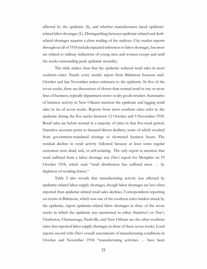
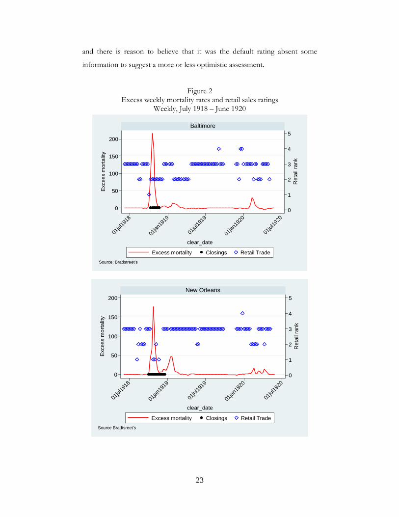
The result appears in Figure 2. The most common summary rating is “good,”
23
and there is reason to believe that it was the default rating absent some
information to suggest a more or less optimistic assessment.
Figure 2 Excess weekly mortality rates and retail sales ratings
Weekly, July 1918 – June 1920
0
1
2
3
4
5
Ret
ail r
ank
0
50
100
150
200
Exce
ss m
orta
lity
01jul
1918
01jan
1919
01jul
1919
01jan
1920
01jul
1920
Baltimore
Excess mortality Closings Retail Trade
clear_date
Source: Bradstreet's
0
1
2
3
4
5R
etai
l ran
k
0
50
100
150
200
Exce
ss m
orta
lity
01jul
1918
01jan
1919
01jul
1919
01jan
1920
01jul
1920
New Orleans
Excess mortality Closings Retail Trade
clear_date
Source Bradtsreet's

24
Figure 2 present the results for two of the South’s largest cities:
Baltimore and New Orleans. (Diagrams for five other cities appear in the
appendix.) The red line (left axis) plots the city-level excess mortality rate; the
blue diamonds (left axis) plot the weekly retail ratings; and the black circles on
the abscissa signify the weeks in which local health authorities ordered closings
of schools, churches, or businesses (NPIs). Excess mortality peaks in mid-
October across the South, with less deadly secondary outbreaks between
December 1918 and February 1919 and again in February 1920. The NPIs, as
Bootsma and Ferguson (2007) and Markel et al (2007) document, were
implemented as mortality moved toward the peak and stayed in place for a few
weeks.
A pattern that repeats across cities is that the retail ratings fall in weeks
when the local health authorities shut down high-risk businesses, namely
restaurants, bars, saloons, and theaters. A second feature is that the retail
ratings also decline during the secondary recurrences when no business
closings were mandated. It is likely that the declines in retail activity during the
second-wave outbreaks are endogenous demand-side responses; that is, people
who are sick or afraid of becoming so choose to avoid public spaces, including
retail spaces, with high risks of disease transmission. Narrative accounts, in
fact, remark on reduced activity in department stores, dry goods stores, and
other retailers selling nonessential goods. Grocers and pharmacies experienced
smaller sales declines.
Figure 3 presents a comparable diagram for manufacturing activities in
the same six southern cities. The red line plots excess mortality, the black
circles the implementation of NPIs, and the blue diamonds in the field the
summary ratings of manufacturing (slow = 1; fair = 2; good =3; active = 4).
The default rating was active, which may have been the result of war-time
demands, and there is less variation in the manufacturing than in the retail
ratings, especially in Atlanta, New Orleans, and Nashville. There is, however,
substantial variation in Baltimore, Louisville, and Memphis.

25
Figure 3 Excess weekly mortality rates and manufacturing activity ratings
Weekly, July 1918 – June 1920
To determine whether there is a statistical relationship between
Bradstreet’s retail and manufacturing ratings and the implementation of NPIs or
0
1
2
3
4
5
Mfg
rank
0
50
100
150
200Ex
cess
mor
talit
y
01jul
1918
01jan
1919
01jul
1919
01jan
1920
01jul
1920
Baltimore
Excess mortality Closings Mfg activity
clear_date
Source: Bradstreet's
0
1
2
3
4
5
Mfg
rank
0
50
100
150
200
Mfg
rank
01jul
1918
01jan
1919
01jul
1919
01jan
1920
01jul
1920
New Orleans
Excess mortality Closings Mfg activity
clear_date
Source: Bradstreet's

26
excess mortality rates, I estimated a seven-city panel fixed-effects logistic
regression equation of the following form:
𝑚𝑚 = log �𝑝𝑝
1 − 𝑝𝑝� = 𝛼𝛼𝑗𝑗 + 𝛽𝛽𝑁𝑁𝑁𝑁𝑁𝑁𝑗𝑗𝑗𝑗 + 𝛾𝛾𝐸𝐸𝐸𝐸𝐸𝐸𝑗𝑗𝑗𝑗 + 𝜀𝜀𝑗𝑗𝑗𝑗 ,
where p is the probability (=1) of a rating of 3 or better, zero otherwise; NPI
indexes those dates when a nonpharmaceutical intervention was in place; EMR
is the city-level excess mortality rate at time t in city j; α is a series of city fixed
effects, and ε is the error term. No other controls are included in the
regressions and the estimates can be viewed as causal only to the extent that
the city fixed effects capture all the relevant time-invariant influences, and the
city-invariant temporal effects are small. Though neither condition seems
likely, regressions at least point toward whether NPIs and endogenous
responses to excess mortality rates had independent effects on retail and
manufacturing activity.
< Table 3 about here >
Table 3 reports the summary statistics of the variables, the estimated
regression coefficients, and marginal effects. The retail ratings for the seven-
city panel are 3 or higher for 74.6% of the retail observations and 80.4% of the
manufacturing observations. In the period between 29 June 1918 and 27 May
1920, local health authorities issued closing orders (NPIs) for 10.2% of weeks.
Excess mortality is 7.9 per 100,000 on average, but the standard deviation
reveals what is evident in Figures 2 and 3, namely that the value is close to zero
except during the three outbreaks. The minimum value of excess mortality is
–5.9; the maximum is 215.7.
The regression coefficients and marginal effects are consistent with a
large, but statistically insignificant negative impact of nonpharmaceutical
interventions on both retail and manufacturing activity. The estimated
marginal effect of NPI in the retail regression suggests that mandated closings

27
reduced the probability of retail being rated “Good” or “Active” by 5.3%.
Mandated closings reduced the probability of manufacturing receiving the
same ratings by 4.5%.
The standard approach is to interpret coefficient (and marginal effects)
estimates evaluated at the mean, but in this case the mean of the excess
mortality rate may not be as informative as other values. A kernel density plot
of excess mortality, in fact, shows a distribution with a mass between –3 and
+3, and a long right tail (see Appendix Figure A.3). It may be easier to interpret
the marginal effect of the pandemic at a handful of critical points in the
distribution, which appear at the bottom of Table 3. There is a 55.2%
probability of observing a retail rating of “Good” or higher when the excess
mortality rate (EMR) is -5. The probability declines to 43.6% at an EMR of
+5, and 23.2% at an EMR of +25, the last of which is consistent with mortality
rates in all cities during the second- and third-wave outbreaks in early 1919 and
early 1920.
Turning to manufacturing ratings, the probability of observing a rating
of “Good” or higher declines by 4.5% when local authorities issued shutdown
orders. Evaluated at the same three points in the distribution used to analyze
the retail rankings, the estimates imply that the probability of observing a
“Good” or higher manufacturing rating is 51.9% when the EMR is –5. When
the EMR is +5, the probability declines to 47.1%, and falls to 37.6% when the
EMR is +25. The likelihood of observing the standard manufacturing rating
declines by about 12 percentage points when the excess mortality rate rises
from normal (=0) to second-wave (=25) levels.
Absent detailed worker- and firm-level data, it is difficult to translate a
12 percentage-point decline in probability of observing a “Good” rating into
economic costs. Estimates of modern data and some back-of-the-envelope
calculations might offer some sense of the costs, at least to an order of
magnitude. First, about one-third of the population was infected by the
Spanish flu, which is about ten times the incidence of influenza-like illness in
a typical flu season and case fatality rates in 1918 were about 25 times greater
than is typical (i.e., 2.5% case fatality in 1918 versus 0.1% in a typical flu season)

28
(Taubenberger and Morens 2006; Akazawa et al 2003). Second, Akazawa et al
(2003) estimate that the incremental effect of contracting an influenza-like
illness in a typical flu season translates into an additional 1.3 days per person
missed at work with a per person cost in 2019 dollars of about $250 (≈ $3 - $6
in 1918, see Williamson 2020). If the greater virulence and morbidity
associated with the Spanish flu is consistent with 10 times as many days missed
and the average daily manufacturing wage was (conservatively) $3.25 in 1918
and per-worker manufacturing income was (conservatively) $810 in 1918, then
the economic cost of the pandemic in lost work days was 5.2% of gross per-
worker income or 5.7% of per-capita gross domestic product.10 Descriptions
of three critical southern industries that follow in subsequent sessions point to
many manufacturing workers missing two to three weeks of work due to
worker sickness, self-isolation, or mandated shutdowns. The pandemic took a
substantial toll on manufacturing output, which was mostly labor-supply
driven.
5.3 ‘Conditions in the mines have been tragic’: Labor supply and coal production
Coal mining was risky in many dimensions: explosions, mine collapses,
debilitating later-life black lung disease. An under-appreciated danger to a
collier’s well-being was the risk of contracting an infectious disease. In 1830s
England, John Snow, a founder of modern epidemiology, treated cholera
victims at the Killingworth Colliery outside Newcastle, and believed that poor
sanitary conditions in mines helped spread the disease (Johnson 2006). It was
conducive, too, to the spread of the flu. Once the influenza pandemic passed,
Metropolitan Life Insurance Company found that 6.2% of all the coal miners
it insured between the ages of 25 and 45 died. By comparison, 3.3% of all
insured industrial workers in that age group died, which was comparable to the
death rates in hard-hit army camps (Metropolitan Life 1920, Barry 2018, 362).
Coal mining demanded strong backs and close contact, which put the most
10 Estimates are derived from following estimates available at Williamson (2020): production worker hourly compensation in 1918 = $0.36; per capita GDP = $732.35. If we assume a nine-hour workday in 1918 and a 250-day work year, per worker gross income is $810.

29
susceptible demographic group – young men – at particular risk. But coal was
vital to the war effort. Even as mine managers and federal officials watched
the death toll mount in the South’s coal fields, it’s digging went on.
Because of coal’s importance, the United States Fuel Administration,
after surveying individual mines in the principal coal-producing regions,
established quotas as a percentage of seasonally adjusted maximum daily
output. The Fuel Administration’s target was 2.1 million tons per day between
1 April and 30 September 1918, and 1.97 million tons per day between 1
October 1918 and 31 March 1919 (Coal Trade Journal, 7 August 1918, 974). The
United States Geological Survey was given the task of surveying firms and
collating the statistics. Beginning 6 April 1918, a trade journal published weekly
summaries of coal production by region. As part of the report it also published,
in tabular form, reasons for the shortfall from targeted production. The table
listed the estimated percent of any shortfall (most weeks the mines reported
less than maximum or required output) attributed to rail car shortages, labor
shortages, strikes, mine disability (disruptions due to required maintenance or
safety concerns), and lack of market. During the war the last listed cause was
almost always zero, given industrial and military fuel demands; strikes were
rare in wartime coal fields. A shortage of able-bodied men due to the draft
created a persistent baseline labor shortage, but this was built into the Fuel
Administration’s capacity estimates. The epidemic, on the other hand, created
acute short-term shortages. Men stayed home because they were sick. Some
surely stayed home because they feared contracting the virus.
Weekly values of output, labor shortage percentages, along with total
US production, and rail car loadings by 123 principal coal-carrying railroads
were collected from Coal Trade Journal. On seven reporting dates between 8
June and 20 July 1918, for example, the government reported that coal
production across the US fell short of estimated capacity by 17.4% of expected
output, on average. Nearly 7.3% of the aggregate shortfall was attributable to
rail car shortages, 4.9% to labor shortages, less than 0.1% to strikes, 3.6% to
mine disability, and 0.2% to lack of a market.

30
Coal production is a particularly useful to gauge the magnitude of
supply-side effects of the pandemic because changes in output, given the
government’s military needs, will be almost completely labor-supply driven
rather than firms responding endogenously to changes in demand. The
percentage of output lost due to “lack of market” remains zero, in fact, until
after the Armistice and does not rise above 5% until 4 January 1919, nearly
two months after the Armistice.
Figure 4 Percent coal mining capacity lost to labor shortages
April 1918 – March 1919 Kentucky’s principal mining regions
Figures 4 and 5 plot the percentage of capacity lost attributable to labor
shortages for the South’s two principal coal regions in Kentucky and West
Virginia (graphs for Southwest Virginia and Northern Alabama are similar).
With the exception of Kentucky’s Western Region, which was centered on
Paducah, Kentucky, and the North Alabama Region, the South’s mining
districts are in a triangle approximately defined by Charleston (WV), Knoxville
(TN), and Lexington (KY). The lines in each graph provide the estimated
percentage losses due to labor shortages for the major mining regions within
0
10
20
30
40
50
perc
ent
10feb
1918
21may
1918
29au
g191
8
07de
c191
8
17mar1
919
date
Hazard NE WestS App No mkt
Kentucky regionspercent capacity lost attributable to labor shortage

31
each state. The diamonds plot the losses attributable to no market, and the
vertical line signifies 19 October 1918, which Collins et al (1930) identify as
the national average peak of the influenza epidemic. Though the Coal Trade
Journal (30 October 1918) reported that the Spanish flu was “a little slow in
reaching the rural districts,” its effects were substantial.
Figure 5 Percent coal mining capacity lost to labor shortages
April 1918 – March 1919 West Virginia’s principal mining regions
Pessimism reigned in late October concerning the short- and long-
term consequences of the epidemic. On 30 October the Journal’s account of
the Louisville coal market opened with the somber observation that
“conditions in the mines have been tragic” over the past two weeks. Some
mines were entirely shut down; many others were operating at 50% of capacity.
West Virginia’s Kanawha district mines reported 733 work hours lost, or about
14% of usual, the previous week. In its discussion of the Baltimore market,
the Journal (30 October 1918) reported that “not only are many miners too ill
to work, but the death list is creating a permanent shortage [of skilled mine
labor].” Equally bleak reports appeared until early December, after which the
0
10
20
30
40
50
perc
ent
10feb
1918
21may
1918
29au
g191
8
07de
c191
8
17mar1
919
date
Newriver Pocahontas VolatileFairmont Cumberland No mkt
West Virginia regionsPercent capacity lost attributable to labor shortage

32
Journal’s discussions of market conditions focused on the anticipated short-
term consequences of the peace, many of which foresaw (not inaccurately) an
industry wracked by excess supply, falling prices, and worker layoffs.
Using the data reported to the Fuel Administration, it is possible to
generate some back-of-the-envelope estimates of output lost to influenza
morbidity and mortality. On 28 September 1918, prior to the virus’ appearance
in the mines, the agency reported it had rated weekly capacity for the eleven
southern mining districts to be 3.97 million tons. Most of the districts reached
between 85 and 94% of their targets. All regions reported some output lost to
labor problems between 0.8 and 7.2% of the target. Weighted by each region’s
rated capacity, the labor-related shortfall for the week of 28 September was
5.2% of maximum output, which is about average for the pre-pandemic
period. Once the pandemic appeared in the mining districts, labor-related
losses roughly tripled. For the week of 19 October, labor-related losses were
15.2% of rated capacity and 15.5% for the following week. For the first week
in November labor-related losses rose to 18.8% of capacity. Barry (2018, 349)
reports that about half of heavy industry labor absenteeism was voluntary,
driven by fear of getting sick. If miners responded at the same rates, then about
7 to 10% percent of coal capacity shortfalls was due to workers choosing to
self-isolate. Regardless of the cause of worker absenteeism, a rapid,
unanticipated loss of 10 to 15% of weekly output for three to four weeks
presented logistical and financial challenges for the coal mining industry, the
US Fuel Administration, and the war effort.
The Coal Trade Journal also noted on several occasions that railroads
that served the coal region were also operating short-handed and at reduced
capacity, sometimes by as much as one-third to one-half. On 26 October, for
example, the Journal reported that the Baltimore & Ohio Railroad, which
ordinarily loaded between 2,000 and 2,500 coal cars per week in the southern
mining districts, had been able to load only 1,000 to 1,500 in the past two
weeks because between 40 and 50% of its workers were out sick. These output
reductions are also purely labor supply-side effects: there was no endogenous
demand-side decline in rail car demand to the epidemic. Military and industrial

33
enterprise demands for coal and rail services had, if anything, only increased
in the last months of war. General Pershing, in fact, had personally asked
miners and mine operators to step up; his war machine needed at least 900,000
more tons of coal per month than they had been using in order to prosecute
the war. A columnist in the Coal Trade Journal responded confidently: “He will
get it” (Coal Trade Journal, 30 October 1918). He may have, but only through
the near-heroic efforts of healthy miners willing to report to work.
5.4 ‘A demoralizing effect upon the industry’: Influenza and southern textiles
In 1918 textile mills represented one of the more important pieces of
the South’s industrial base. The industry was located along the eastern foothills
of the Appalachian Mountains from Danville, Virginia through the Carolinas
into northeast Georgia. The South Carolina Upcountry, for example, was
home to about three-quarters of the state’s 170 cotton textile mills, which
operated more than 4.9 million spindles, with a total invested capital of $100
million, value of annual output of $217 million, employed more than 48,000
hands, and paid more than $28.3 million in wages (South Carolina
Commissioner 1918, 55). Thus, when the pandemic appeared in South
Carolina, its cotton mills accounted for more than half of all capital invested
in manufacturing plant and equipment, more than two-thirds of the value of
the state’s industrial output, and nearly two-thirds of all industrial employment
and wages paid to manufacturing workers.
Before the pandemic appeared in the southern textile region, the war
had already made itself felt. A South Carolina report noted that military
inductions had pulled many young men from the mills. “Women who remain
at home,” wrote the state labor commissioner, “keep the home fires burning,
many of them taking up the burden of the family support, and doing so with
great willingness” (South Carolina Commissioner 1918, 4). The commissioner
purposefully struck a patriotic tone, of course, but the facts belie his assertion.
It was true that between 1916 and 1918 the state’s mills increased the real dollar
value of output by about 40% and that the number of males employed by the
mills declined by about 4,500, but the number of females employed also

34
decreased by nearly 400 hands. Fewer textile mill operatives were working
more.
The second war-related influence was the government’s demand for
uniforms and tent canvas. By September 1918 cotton mills across the South
were operating at full capacity. Before the war Dan River Mills, in Danville,
Virginia, typically operated a single 9-hour shift on weekdays. If demand was
unusually large it might run a second shift until large orders were filled. As the
war neared its end in 1918, Dan River was operating three shifts, which kept
its plants operating 24 hours a day (Smith 1960). The Cannon Mills in
Kannapolis, North Carolina, too, operated close to capacity filling orders for
military-grade textiles (Vanderburg 2013). At least through the Armistice and
perhaps beyond, there was no notable decline in demand for cotton textiles
manufactured in the South. Any pandemic-related effect operated through the
labor-supply channel.
Although the industry’s trade journals did not detail the consequences
of the pandemic with the level of detail found in the coal trade journals,
narrative accounts provide some evidence on the timing and magnitude of its
supply-side effects. On 12 October, a Philadelphia jobber returned from a trip
through the South and reported that many mills were “severely handicapped
by the influenza epidemic;” one mill was so short-handed that it was running
just 20 of 300 spinning frames (Textile World Journal, 12 October 1918, 28). A
report dated 9 October from Raleigh, North Carolina, informed the
magazine’s readers that infection rates were so high that some mills were
shutting down voluntarily to slow it’s spread; the report further predicted that
several plants in the Carolinas were closed and likely to remain so for the
“duration of the epidemic” (Textile World Journal, 19 October 1918, 69).
Independent reports from 26 October noted that the epidemic spread “with
alarming quickness” in the mill villages; that about half the regions mills were
either closed or employee absenteeism had been “disastrous;” that mills that
shut down tended to remain so for up to two weeks; and mills that continued
to operate did so with “25 to 50 per cent of their normal complement of help”
(Textile World Journal, 26 October 1918, 67, 73, 83).
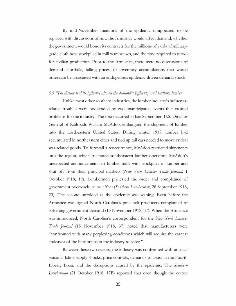
35
By mid-November mentions of the epidemic disappeared to be
replaced with discussions of how the Armistice would affect demand, whether
the government would honor its contracts for the millions of yards of military-
grade cloth now stockpiled in mill warehouses, and the time required to retool
for civilian production. Prior to the Armistice, there were no discussions of
demand shortfalls, falling prices, or inventory accumulations that would
otherwise be associated with an endogenous epidemic-driven demand shock.
5.5 “The disease had its influence also on the demand”: Influenza and southern lumber
Unlike most other southern industries, the lumber industry’s influenza-
related troubles were bookended by two unanticipated events that created
problems for the industry. The first occurred in late September, U.S. Director
General of Railroads William McAdoo, embargoed the shipment of lumber
into the northeastern United States. During winter 1917, lumber had
accumulated in northeastern cities and tied up rail cars needed to move critical
war-related goods. To forestall a reoccurrence, McAdoo restricted shipments
into the region, which frustrated southeastern lumber operators. McAdoo’s
unexpected announcement left lumber mills with stockpiles of lumber and
shut off from their principal markets (New York Lumber Trade Journal, 1
October 1918, 19). Lumbermen protested the order and complained of
government overreach, to no effect (Southern Lumberman, 28 September 1918,
23). The second unfolded as the epidemic was waning. Even before the
Armistice was signed North Carolina’s pine belt producers complained of
softening government demand (15 November 1918, 37). When the Armistice
was announced, North Carolina’s correspondent for the New York Lumber
Trade Journal (15 November 1918, 37) noted that manufacturers were
“confronted with many perplexing conditions which will require the earnest
endeavor of the best brains in the industry to solve.”
Between these two events, the industry was confronted with unusual
seasonal labor-supply shocks, price controls, demands to assist in the Fourth
Liberty Loan, and the disruptions caused by the epidemic. The Southern
Lumberman (21 October 1918, 17B) reported that even though the cotton

36
harvesting season was winding down, white and black sharecroppers, who had
realized high prices for their cotton, were not yet “drifting back to the
sawmills.” In late September, rising production costs and price ceilings made
lumber milling unprofitable for some (Southern Lumberman, 5 October 1918,
24). The region’s lumbermen were taking an active role in the Liberty Loan,
“many of them devoting all of their time to it” Several of the region’s
manufacturers and wholesalers placed either fearmongering or patriotic-
themed, whole-page advertisements in industry trade journals encouraging
people to buy bonds (see Figure 6). At the same time, the influenza “made
itself felt” across the South (Southern Lumberman, 21 October 1918, 17B).
< Figure 6 about here >
The earliest reference in a trade journal to influenza disrupting the
South’s timber and lumber industry appears in early October, at which time a
writer in Southern Lumberman opined: “If the Spanish flu is really Spanish in its
origin, Spain is abundantly getting even with us for what happened twenty
years ago” (Southern Lumberman, 5 October 1918, 23). From then through mid-
November, bi-weekly assessments of the market for North Carolina-grade
pine note the impact of the epidemic. On 14 October, the outbreak was
“raging” and interfered with business (Southern Lumberman, 19 October 1918).
Two weeks later both Southern Lumberman and New York Lumber Trade Journal
reported that sickness was so widespread among mill owners, managers, and
workers that many sawmills were shut down.
Although pine lumber producers in Virginia and the Carolinas
experienced labor-supply shocks, the industries they served were also hard hit
by the virus, which sent ripples through the industry. Furniture factories in
Fayetteville, North Carolina suspended operations due to worker absenteeism
and cancelled orders of better-grade pine. The principal consumers of North
Carolina-grade pine in 1918, however, were makers of wooden boxes used to
ship war materiel to France. At the peak of the epidemic in Baltimore, the
government ordered its box makers to make coffins instead. But box makers

37
could not meet the need because box factory workers were out sick and orders
for box-grade lumber lagged (Southern Lumberman, 26 October 1918 and 2
November 1918). Just as the region’s railroads loaded fewer coal cars than
usual due to worker sickness, at the height of the epidemic pine shipments out
of Norfolk, Virginia were hindered because barge and ship crews were out sick
(Southern Lumberman, 12 October 1918).
Unlike coal and textiles, industries in which supply-side effects
dominated, the South’s lumber millers were buffeted by both demand and
supply shocks. Employees missed work and shipments of low-grade pine
slowed because the government’s war planners determined that stockpiles in
the Northeast were already sufficient. Moreover, the only alternative to rail
transport of its production – shipping on barges through the port at Norfolk
– suffered its own debilitating labor-supply shortages.
6. Southern business failures during the pandemic
Both Dun’s and Bradstreet’s commented repeatedly on the declining
number of business failures during the war, a trend evident in Figure 7. The
plots detail the total number of business failures each week between December
1914 and June 1920 in the four regions used by Dun’s to aggregate and report
the data.
Because Dun’s did not report the number of businesses at risk, it is
impossible to calculate a business failure rate, but the South’s experience stands
out on a per capita basis. The East and Midwest were more populous than the
South and, after the large number of failures in early 1915, the number of
failures in the East, Midwest, and South are comparable. In late June 1916, for
instance, there were 71 failures in the East region, 64 in the Midwest, and 74
in the South. Further, there is no obvious break in any of the series after 26
September 1918 (delineated in the graph), when the pandemic emerged in the
eastern US, or on the announcement of the Armistice five weeks later on 11
November 1918.

38
Figure 7 Business failures by region
December 1914 – June 1920 Source: Dun’s
To determine whether different timing of the pandemic outbreak,
nonpharmaceutical interventions, and the armistice had any effect on regional
failures I estimate a panel fixed effects negative binomial (count) model of
failures in the four regions. The estimated equation takes the following form:
𝑓𝑓𝑚𝑚𝑚𝑚𝑚𝑚𝑗𝑗𝑗𝑗 = 𝛼𝛼 + 𝛽𝛽1𝐸𝐸𝐸𝐸𝐸𝐸𝑗𝑗𝑗𝑗 + 𝛽𝛽2𝑁𝑁𝑚𝑚𝑚𝑚𝑚𝑚𝐸𝐸𝑚𝑚𝑚𝑚𝐸𝐸𝑗𝑗𝑗𝑗 + 𝛽𝛽3�𝑁𝑁𝑚𝑚𝑚𝑚𝑚𝑚𝐸𝐸𝑚𝑚𝑚𝑚𝐸𝐸𝑗𝑗𝑗𝑗 × 𝐸𝐸𝐸𝐸𝐸𝐸𝑗𝑗𝑗𝑗�
+ 𝛽𝛽4𝑁𝑁𝑁𝑁𝑁𝑁𝑗𝑗𝑗𝑗 + 𝛽𝛽5 𝐴𝐴𝑚𝑚𝑚𝑚𝑚𝑚𝐸𝐸𝑚𝑚𝑚𝑚𝐸𝐸𝐸𝐸𝑗𝑗 + 𝛽𝛽6𝑚𝑚𝑚𝑚𝐸𝐸𝑚𝑚𝑚𝑚𝑗𝑗 + 𝛾𝛾𝑗𝑗 + 𝜖𝜖𝑗𝑗𝑗𝑗 ,
Where the dependent variable is the regional failures measured as
integer count data. Pandemic is an indicator variable that takes the value of
one under one of three definitions. The preferred definition is that used by
Markel et al (2007), who define the onset of the pandemic for each US city of
more than 100,000 residents in 1918 as the date at which the excess influenza-
pneumonia mortality rate exceeded twice the baseline rate. I dated the
0
100
200
300
0
100
200
300
01jul
1914
01jul
1916
01jul
1918
01jul
1920
01jul
1914
01jul
1916
01jul
1918
01jul
1920
East Midwest
Pacific South
Failu
res
DateSource: Dun's (various issues), 1915-1920
December 1914 - June 1920Business failures

39
beginning as the average of the dates for the cities in each of the four regions
(see Appendix Table A1 for dating by city and region), and the end as the date
at which the excess mortality rate falls below twice the baseline rate for four
or more consecutive weeks. A second definition (Pandemic 2) takes a value of
one for the period between 26 September 1918 and 30 June 1920. A third
definition (Pandemic 3) takes a value of one for every date after 26 September
1928 through the end of the sample.
NPI is an indicator variable that equals one during the average
mandated closure dates by region. There is regional variation in dates because
NPIs were imposed later (albeit earlier relative to the initial influenza reports)
and kept in place longer in the Pacific region than elsewhere. Armistice is an
indicator variable that equals one after 11 November 1918. For regional
EMR’s, I use the excess mortality rates of one representative city for each
region: Albany for the East, Richmond for the South, Omaha for the Midwest,
and Portland for the Pacific. The choice of city should make little difference.
The correlation between the Richmond data, for instance, and every southern
city in the Collins et al (1930) data, with the exception of Atlanta, has a
correlation coefficient of 0.90 or higher. The model is estimated as a panel
region fixed-effects model. The estimates are qualitatively the same with or
without the linear trend variable.
Estimated coefficients on the interaction between Pandemic and
excess mortality rate can be thought of as a type of continuous treatment
difference-in-differences effect, where the treatment is the regional excess
mortality rate, interacted with one of three “post” periods of interest (as in
Fang et al 2020). The excluded period includes all dates prior to the outbreak
of the pandemic, and for certain periods after the pandemic, depending on its
specific definition.
< Table 4 about here >
Table 4 provides summary statistics for the four-region panel. The
average week saw 63 business failures, though there was substantial regional

40
and temporal variation. The South, for instance, experienced more than 300
failures in early 1915. Weekly average excess mortality was 2.59 per 100,000,
but as Appendix Figure A1 makes clear, the mass of the distribution was
centered on zero with a long right tail. Given EMR’s non-normal distribution
and because negative numbers are a natural realization, the data is transformed
using the inverse hyperbolic sine function, which approximates the natural log
transformation for positive realizations; it maps zero into zero, and transforms
negative values into negative values absent an arbitrary adjustment, as is
customarily done with log transformations (Bellemare and Wichman 2019 note
that there are subtleties to interpreting estimated coefficients from
transformed as elasticities). Nonpharmaceutical interventions were in effect
during 6% of the sample dates. By the narrowest (and preferred) definition,
the pandemic raged for 10% of the dates, or about 28 weeks. This definition
is closest to Cross et al’s (1930) dating; by their estimates, the pandemic
persisted for 31 weeks after 12 September 1918. Alternative definitions date
the pandemic for nearly one-third of the sample dates, as does the Armistice
variable.
< Table 5 about here>
Table 5 presents incidence rate ratios (IRRs) from the panel negative
binomial regressions. Estimated incidence ratios imply that a one-unit increase
in the excess mortality rate (i.e., one more influenza-related death per week
above the baseline per-pandemic rate) increased the business failure rate by a
factor of approximately 1.03, or about 3 percent, across all specifications. In
column (2) the interaction term between the Pandemic and EMR variable
implies that, for a one-unit increase in excess mortality, the number of business
failures decreased by a factor 0.94 or about 6% during the pandemic proper.
It is notable that the implementation of nonpharmaceutical interventions, for
a few weeks, and the announcement of the Armistice, up to the end of June
1920 at least, are associated with a decrease in the number of business failures.
Under alternative definitions of the pandemic, the effect of the Armistice is

41
positive but insignificant, which may be due to the near concurrence of dates
for Pandemic 3 and Armistice.
The bottom line is that neither nonpharmaceutical interventions nor
the Armistice had much effect on business failures in the weeks (or months)
surrounding the pandemic. It is possible that the decline in business failures
during the pandemic and the mandated closures may be a consequence of
courts being closed, as well as businesses, which may have delayed bankruptcy
filings by a few weeks.
A second question that arises with respect to business failures is the
sectoral composition of failures. During COVID-19 lock downs in 2020 retail,
travel, and restaurants experienced large sales declines. It is useful to
understand what happened during the Spanish flu pandemic, knowing that
public health authorities closed mostly high-contact, nonessential businesses
such as taverns, theaters, restaurants, and so on. Dun’s parsed its monthly
failure reports into three broad categories: manufacturing, retail, and finance.
It further subdivided each category into more narrowly-defined sectors. In
manufacturing it reported data for machinery, textiles, milling, and others, as
well as an aggregate numbers and liabilities for manufacturing. In retail Dun’s
reported separate accounts for general stores, grocers, dry goods, liquor and
tobacco, hotels and restaurants, and clothing, among others, as well as all retail
failures and their aggregate liabilities. Dun’s failure accounts did not parse
failures by region and sector, but there is no reason to think that the sectoral
composition of urban retail in the South would have differed markedly from
other regions. Southern manufacturing, however, was different; textiles and
agricultural and natural resource processing, such as tobacco, cottonseed oil,
and lumber were the region’s principal manufacturing industries.
Figure 8 presents the aggregate number of failures and real liabilities
per failure for the manufacturing and retail sectors. (Liabilities per failure are
adjusted for inflation using the Warren-Pearson index and manufacturing
liabilities are divided by 10 to simplify the graph.) As is evident in the regional
data, business failures declined from the outbreak of the First World War up
to the postwar recession that began in the second half of 1920. There is no

42
obvious break in the aggregate number of failures around the pandemic in mid-
September 1918. Average liabilities per failure, on the other hand, appears to
increase around the pandemic in both manufacturing and retail.
Figure 8 Business failures and liabilities per failure, 1916-1920
To better understand the causes of failures, I estimate negative
binomial regressions on the count failure data and OLS regressions on
aggregate sectoral liabilities on the fine-grained sector definitions using
monthly data. The results cannot be interpreted as causal in nature; rather, they
are designed to serve as a preliminary investigation of different sectoral
responses to the pandemic and mandated closures. For each sector, I estimate
regressions of the following general form:
𝑚𝑚𝑗𝑗𝑗𝑗 = 𝛼𝛼 + 𝛽𝛽1 𝑁𝑁𝑚𝑚𝑚𝑚𝑚𝑚𝐸𝐸𝑚𝑚𝑚𝑚𝐸𝐸𝑗𝑗 + 𝛽𝛽2 𝑁𝑁𝑁𝑁𝑁𝑁𝑗𝑗 + 𝛽𝛽3𝐴𝐴𝑚𝑚𝑚𝑚𝑚𝑚𝐸𝐸𝑚𝑚𝑚𝑚𝐸𝐸𝐸𝐸𝑗𝑗 + 𝛽𝛽4 𝑚𝑚𝑚𝑚𝐸𝐸𝑚𝑚𝑚𝑚
+ 𝐸𝐸𝑗𝑗𝑗𝑗 ,
The outcome variable, y, is either count failure data or the natural log
of liabilities per failure. Pandemic is measured as either the inverse hyperbolic
0
500
1000
1500
Num
ber o
f fai
lure
s
12mar1
916
25jul
1917
07de
c191
8
20ap
r1920
Date
Manufacturing Retail
Business failures
0
2000
4000
6000
8000
Dol
lar l
iabi
litie
s
12mar1
916
25jul
1917
07de
c191
8
20ap
r1920
02se
p192
1
Date
Manufacturing/10 Retail
Liabilities per failure

43
sine of national average excess mortality as reported in Cross et al (1930) or as
a dummy variable equal to one between September 1918 and March 1919.
Nonpharmaceutical interventions (NPI) is a noisy dummy variable equal to
one between October and December 1918, which captures the approximate
dates of business shutdowns in the US; they occurred about two weeks later
and lasted about a month longer in the Pacific region. Because NPIs cannot
be accurately captured with national data, any estimated coefficient on NPI
will be attenuated. Armistice is a dummy variable equal to one after November
1918. The regressions also include a linear trend.
Table 6 provides the summary statistics for the count failure data
sample. Retail enterprises reported more failures than manufacturing
enterprises. In a typical month 252 manufacturing establishments closed; 626
retailers did so. Nearly 200 grocers failed each month on average, compared
to just 17 machine shops.
Table 7 reports incidence rate ratios from negative binomial
regressions on the monthly failure count data by narrow sector, as well as the
broader manufacturing and retail categories. Generally, the regressions explain
only a small fraction of the variance for manufacturing failures; they explain
substantially more of the variance in retail establishment failures. Among the
principal manufacturing sectors, pandemic-era events are associated with
modest and mostly insignificant effects on enterprise failures.
In the retail sector (Panel B), there is some limited evidence of an
association between pandemic events and business failures. The exponentiated
constants imply that there was an average of 130.3 failures of general stores
each month and 322.3 grocery failures. The incidence ratios on the inverse
hyperbolic sine of excess mortality in a majority of the regressions, as well as
for the overall retail sector, are consistent with an increase in failures of about
1 to 5% for a one arcsin-point increase in excess mortality (∆EMR ≈ 1.2); an
increase consistent with a pandemic-like spike in mortality increases failures by
about a factor of 3, or about 3 to 15%. General stores, clothing, and dry goods
– all of which might be considered sellers of nonessential consumer goods –
suffered the largest increase in failures. Grocers and liquor stores experienced

44
lesser effects. Mandated closings (NPIs) had consistently large and negative
effects on contemporaneous retail failures, which, again, might be a
consequence of the courts, too, having closed during the pandemic. The
announcement of peace in November is not associated with an increase in
business failures among either manufacturers or retailers.
< Table 8 about here >
Table 8 provides summary statistics for the aggregate liabilities of
failing firms for the same sectors included in the count data. The average
aggregate real monthly liabilities of failing machine shops were just less than
$500,000; the highest monthly aggregate exceeded $1.7 million. The average
aggregate liabilities of monthly failures in the retail sector was about $300,000;
the liabilities of liquor store failures were less, grocery failures more.
< Table 9 about here >
Table 9 presents coefficient estimates from OLS regressions of the
natural log of real monthly liabilities on the natural log of the excess mortality
rate, an NPI dummy, and an Armistice dummy. The log-arcsin specification
means that the estimates can be loosely interpreted as the elasticity of failed
business liabilities with respect to the excess mortality rate (Bellemare and
Wichman 2019). The estimated elasticities are not large and only three are
statistically significant at the 5% level. It is interesting, however, that the
elasticities for all manufacturing and all retail establishments are significant and
imply that a 10% increase in excess mortality leads to a 5.7% increase in the
liabilities of failing manufacturing firms and a 4.0% increase in the liabilities of
failing retail firms. There is no discernible pattern to the coefficients on NPI
or Armistice. If, instead, we are interested in the average size of failing firms,
a 10% increase in excess mortality leads to a statistically significant increase in
the average size of failing manufacturers of 5.2%; the effect on average retail
failures is smaller (1.8%) and insignificant (results not tabulated).

45
Overall, the evidence on business failures suggests that neither the
pandemic nor government-mandated closures had a marked effect on business
failures. Increases in the excess mortality rate is associated with a modest
increase in the number of failures. No narrow sector of the economy, such a
leisure or entertainment, appears to have experienced an adverse effect. That
is, despite mandated closures of restaurants, taverns, and theaters, among other
businesses, failure rates in these lines of business did not increase. The absence
of a discernible effect may be due to several factors: noncompliance with
closure orders; the relative brevity of the closures; and that many sectors of
the economy continued to operate at something as close to capacity as
possible, given the labor supply shocks due to sick and fearful workers not
showing for work, during a period when the US government was committed
to prosecuting total war in Europe fully aware of its domestic consequences.
7. Concluding comments
In his depiction of London’s 1854 cholera epidemic, during which the
Golden Square section of the city witnessed more than 500 deaths in ten days,
John Snow, one of the founders of modern epidemiology, observed that the
death rate would have been much higher had it not been for the “flight of the
population” (quoted in Johnson 2006, 169). Still-healthy residents picked up
and left. Some tradesmen closed down their storefronts; the ones who stayed
open sent their families away. “The most afflicted streets,” Snow wrote, “were
deserted by more than three-quarters of their inhabitants.” Unlike cholera
outbreaks, which tend to be localized, the Spanish flu afforded no place to run.
The virus killed in major cities and small towns. Even mining camps in remote
Kentucky coal fields sometimes buried 10% or more of their residents (Barry
2018). With nowhere to run from the flu, the only protection was to hide – or,
in modern terms, to self-isolate.
It is hard to determine how many people self-isolated or for how long
during the Spanish flu epidemic. Epidemiological models that incorporate
endogenous responses imply nontrivial responses to COVID-19, which
necessarily reduces infections and deaths. Daniel Defoe and John Snow

46
recognized this effect long before it was the object of mathematically rigorous
exercises. This study finds that the effects of pandemic-induced closings,
sickness, and self-isolation on business were substantial, if short-lived. Some
coal mines and textile mills, for example, continued to operate with worker
absenteeism rates of 20 to 50%; output declined, for a few weeks at least, by
an estimated 10 to 15%. These values are consistent with Barro at al’s (2020)
estimates, which place the Great Pandemic as the fourth most economic costly
event of the twentieth century. Their estimates point to a 6% decline in GDP
and 8% decline in consumption. A simple back-of-the-envelope calculation
using the values reported here – four weeks (=8% of the work-year) times 50%
loss of worker wages due to absenteeism – points to a 4% loss in aggregate
per-worker income in large sectors of the southern economy. Thus, the effects
of the pandemic documented here are of the same order of magnitude as
theirs. More importantly, perhaps, is the finding that the losses were due
primarily not to mandated business closures, which were short lived, easily
evaded and narrowly targeted, but to the widespread incidence of influenza
and the resulting reduction in labor hours. Lockdowns are economically costly
in the short term, but so too are spikes in influenza-related morbidity and
mortality.

47
References
Akazawa, Manabu, Jody L. Sindelar, and A. David Paltiel. 2003. Economic
costs of influenza-related work absenteeism. Value in Health 6(2), 107-
115.
Alabama Department of Public Health (ADPH). 2017. 1918 influenza in
Alabama timeline. Available at
https://www.alabamapublichealth.gov/pandemicflu/1918-influenza-
timeline.html. Accessed May 2020.
Almond, Douglas. 2006. Is the 1918 influenza pandemic over? Journal of Political
Economy 114(4), 672-712.
Bainbridge, Judy. 2019. How the 1918 Spanish flu pandemic gripped
Greenville, South Carolina. Greenville News (5 January 2019).
Barro, Robert J., J. F. Ursúa, and J. Weng. 2020. The coronavirus and the great
influenza pandemic: lessons from the Spanish flu for the coronavirus’s
potential effects on mortality and economic activity. NBER wp 26866.
Barry, John M. 2018. The Great Influenza: The Story of the Deadliest Pandemic in
History. New York: Penguin Books.
Bellemare, Marc F. and Casey J. Wichman. 2019. Elasticities and the inverse
hyperbolic sine transformation. Working paper, University of
Minnesota.
Blickle, Kristian. 2020. Pandemic change cities: municipal spending and voter
extremism in German, 1918-1933. Federal Reserve Bank of New York Staff
Reports No. 921. GET PERMISSION TO CITE THIS
Bootsma, Martin C. J., and Neil M. Ferguson. 2007. The effect of public health
measures on the 1918 influenza pandemic in U.S. cities. Proceedings of
the National Academy of Sciences 104(18), 7588-7593.
Bradstreet’s: A Journal of Trade, Finance, and Public Economy. 1917-1919. New York:
Bradstreet Company.
Brainerd, E. and M. V. Siegler. 2003. The economic effects of the 1918
influenza epidemic. CEPT Discussion Papers 3791.

48
Bureau of Labor Statisics (BLS). 2020. The employment situation – April 2020.
Available at https://www.bls.gov/news.release/pdf/empsit.pdf.
Accessed 10 May 2020.
Burns, Arthur F. and Wesley Claire Mitchell. 1946. Measuring Business Cycles.
New York: National Bureau of Economic Research.
Center for Disease Control (CDC). 2020. COVID-19 forecasts. Available at
https://www.cdc.gov/coronavirus/2019-ncov/covid-
data/forecasting-us.html. Accessed 10 May 2020.
Coal Trade Journal. 1918-1919. New York.
Cockrell, David L. A blessing in disguise: the influenza pandemic of 1918 and
North Carolina’s medical and public health communities. North
Carolina Historical Review 73(3), 309-327.
Collins, Selwyn D., W. H. Frost, Mary Gover, and Edgar Sydenstricker. 1930.
Mortality from influenza and pneumonia in 50 large cities of the
United States, 1910-1929. Public Health Reports 45(39), 2277-2330.
Correia, Sergio, Stephan Luck, and Emil Verner. 2020. Pandemics depress the
economy, public health interventions do not: evidence from the 1918
flu. Working paper. Available at https://ssrn.com/abstract=3561560.
Culver, Gregory K. 1991. The impact of the Spanish influenza epidemic on
the Jackson Purchase. Filson Club Historical Quarterly 65(4), 487-504.
Defoe, Daniel. 1904 (1772). A Journal of the Plague Year. London and New York:
The Chesterfield Society.
Dun’s Review: A Journal of Finance and Trade, Domestic and Foreign. 1916-1919. New
York: R. G. Dun & Company, The Mercantile Agency.
Eichenbaum, M. S., S Rebelo, and M. Trabandt. 2020. The macroeconomics
of epidemics. NBER wp 26882.
Fang, Hanming, Long Wag, and Yang Yang. 2020. Human mobility
restrictions and the spread of the novel coronavirus (2019-NCov) in
China. NBER working paper no. 26906.
Fernández-Villaverde, Jesús and Charles I. Jones. 2020. Estimating and
simulating a SIRD model of COVID-19 for many countries, states,
and cities. NBER wp #.

49
Finger, Michael. 2011. The return of the Spanish lady? Memphis: The City
Magazine (Nov/Dec 2011). Available at
https://memphismagazine.com/features/the-return-of-the-spanish-
lady/. Accessed May 2020.
Garrett, Thomas A. 2007. Economic effects of the 1918 influenza pandemic:
implications for a modern-day pandemic. Federal Reserve Bank of St.
Louis. Available at www.stlouisfed.org/community/other_pubs.html.
Accessed April 2020.
Guimbeau, Menon, and Aldo Musacchio. 2020. The Brazilian bombshell? The
long-term impact of the 1918 influenza pandemic the South American
way. NBER wp 26929.
Johnson, Steven. 2006. The Ghost Map: The Story of London’s Most Terrifying
Epidemic – and How it Changed Science, Cities, and the Modern World. New
York: Riverhead Books.
Jordá, Osca, Sanjay R. Singh, and Alan M. Taylor. 2020. Longer-run economic
consequences of pandemics. NBER wp 26934.
Karlsson, Martin, Therese Nilsson, and Stefan Pichler. 2014. The impact of
the 1918 Spanish flu epidemic on economic performance in Sweden:
an investigation into the consequences of an extraordinary mortality
shock. Journal of Health Economics 36(1), 1-19.
Kermack, William O. and A. G. McKendrick. 1927. A contribution to the
mathematical theory of epidemics, part I. Proceedings of the Royal Society
of London, Series A 115(772), 700-721.
Lilley, Andrew, Matthew Lilley, and Gianluca Rinaldi. 2020. Public health
interventions and economic growth: revisiting the Spanish flu
evidence. Working paper, Harvard University. Available at
https://ssrn.com/abstract=3590008.
Markel, Howard, et al. 2007. Nonpharmaceutical interventions implemented
by US cities during the 1918-1919 influenza pandemic. JAMA 298(6),
644-654.
Markel, Howard, et al. 2007. Nonpharmaceutical interventions implemented
by US cities during the 1918-1919 influenza pandemic. Appendices

50
and supplementary materials. (Includes dates of school and business
closures, etc.). Available at:
http://chm.med.umich.edu/research/nonpharmaceutical-
interventions-implemented-by-us-cities-during-the-1918-1919-
influenza-pandemic/
Markel, Howard, et al. 2007. Nonpharmaceutical interventions implemented
by US cities during the 1918-1919 influenza pandemic. Appendices
and supplementary materials. (Includes dates of school and business
closures, etc.). Available at:
https://web.archive.org/web/20090927163944/http:/www.cdc.gov/
ncidod/dq/1918_flu_supp.htm
Maupin, Judith Ann. 1975. The Spanish influenza epidemic in West Kentucky.
Jackson Purchase Historical Society 3(1), 44-55.
McLaurin, Ann. 1982. The influenza epidemic of 1918 in Shreveport. North
Louisiana Historical Association Journal 13, 1-14.
Metropolitan Life Insurance Company. 1920. Statistical Bulletin.
Percoco, Marco. 2016. Health shocks and human capital accumulation: the
case of the Spanish flu in Italian regions. Regional Studies 50(9), 1496-
1508.
Plaspohl, Sara S., Betty T. Dixon, and Nyssa Owen. 2016. The effect of the
1918 Spanish influenza pandemic on mortality rates in Savannah,
Georgia. Georgia Historical Quarterly 100(3), 332-339.
Rosner, David. 2010. Spanish flu, or whatever it is…: the paradox of public
health in a time of crisis. Public Health Reports 125(Supplement 3), 38-
47.
Scott, Kim Allen. 1988. Plague on the homefront: Arknasas and the great
influenza epidemic of 1918. Arkansas Historical Quarterly 47(4), 311-344.
Slosson, Preston William. 1930. The Great Crusade and After. New York:
Macmillan Company.
Smith, Robert S. 1960. Mill on the Dan: A History of Dan River Mills, 1882-1950.
Durham, N.C.: Duke University Press.

51
South Carolina Commissioner of Agriculture, Commerce and Industries. 1918.
Tenth Annual Report of the Commissioner of Agriculture, Commerce and
Industries: Labor Division. Columbia: Gonzales & Bryan, State Printers.
Taubenberger, Jeffrey K. and David M. Morens. 2006. 1918 influenza: the
mother of all pandemics. Emerging Infectious Diseases 12(1), 15-22.
Textile World Journal: A Journal of News, Market Reports and Technical Information.
1918-1919. New York Textile World Journal Company.
Thanner, Meredith H., Jonathan M. Links, Martin I. Melzner, James J.
Scheulen, and Gabor D. Kelen. 2011. Understanding estimated worker
absenteeism rates during an influenza pandemic. American Journal of
Disaster Medicine 6(2), 89-105.
Torry, Harriet. 2020. Stores, factories hit by lockdown. Wall Street Journal (16
May, A1).
Vanderburg, Timothy W. 2013. Cannon Mills and Kannapolis: Persistent Paternalism
in a Textile Town. Knoxville: University of Tennessee Press.
Velde, François R. 2020. What happened to the US economy during the 1918
influenza pandemic? A view through high-frequency data. Working
paper, Federal Reserve Bank of Chicago.
Wheelock, David C. 2020. What can we learn from the Spanish flue pandemic
of 1918-19 for COVID-19. Federal Reserve Bank of St. Louis Economic
Synopses 30, 1-4.
Williamson, Samuel H. 2020. Seven ways to compute the relative value of a
U.S. dollar amount, 1790 to present. Available at
https://www.measuringworth.com/calculators/uscompare/relativev
alue.php.
Wirth, Thomas. 2006. Urban neglect: the environment, public health, and
influenza in Philadelphia, 1915-1919. Pennsylvania History: A Journal of
Mid-Atlantic Studies 73(3), 316-342.
Woolley, Ivan M. 1963. The 1918 Spanish influenza pandemic in Oregon.
Oregon Historical Quarterly 64(3), 246-258.

52
Table 1 Nonpharmaceutical interventions in southern cities
City First case date
First intervention
date
Intervention days
Source
Atlanta, GA
10/7 29 Bootsma (2007) Baltimore, MD 9/18 10/9 43 Markel (2007)
Birmingham, AL 9/24 10/9 48 Markel (2007) Greenville, SC 9/17 10/7 28 Bainbridge (2019) Huntsville, AL 9/28 10/7
ADPH (2017)
Little Rock, AR 9/20 10/6 29 Scott (1988), Finger (2011) Louisville, KY 9/13 10/7 145 Markel (2007) Memphis, TN 9/25 10/10 20 Finger (2011) Nashville, TN 9/21 10/7 55 Markel (2007)
New Orleans, LA 9/10 10/8 78 Markel (2007) Paducah, KY 9/18 10/8 35 Maupin (1975)
Richmond, VA 9/21 10/6 60 Markel (2007) Shreveport, LA 9/27 10/8 38 McLaurin (1982)
Washington, DC 9/11 10/3 64 Markel (2007) Wilmington, NC 9/19 10/10 by year end Cockrell (1996)

53
Table 2 Dun's and Bradstreet’s notes of epidemic and its effects
Oct 12 Oct 19 Oct 26 Nov 2 Nov 9 Nov 16 Nov 23
Baltimore C S L C C S L S L S S Richmond S L S L S Lynchburg Wheeling S S L S S
Wilmington S Charleston S L S L C S L S Louisville L C S Memphis C S C L S L Q S S L Nashville C S L S L
Chattanooga L S L S S L Atlanta C C S S S
Birmingham L New Orleans S L S C S L S C S L S
Mobile C S L S
Sources: B, 651 B, 667 B, 682 B, 699 B, 715 B, 731 B, 747 D,726 D, 743 D, 757 D, 771 D, 785 D, 799 D, 813
Notes: S = retail/wholesale sales affected; L = mfg labor affected; C = business closings; Q = quarantine, partial or complete; Green shades = influenza mentioned Sources: Key B = Bradstreet’s (1918), page number; D = Dun’s (1918), page number.

54
Table 3 Business activity ratings, nonpharmaceutical interventions, and excess mortality
Summary statistics
Logit regressions
Dependent variables Mean
Retail marginal effects
Manufacturing marginal effects
(Std dev)
Retail rating (0/1) 0.746
(0.436)
Manufacturing rating 0.804
(0.397)
Independent variables
NPI 0.102
-0.229 -0.053 -0.188 -0.045 (0.304)
(0.448)
(0.510)
Excess mortality 7.909
-0.047 -0.011 -0.019 -0.005 (20.946)
(0.011)**
(0.007)**
Pr(rating=1|ERM)
EMR = -5
0.552
0.519
EMR = 0
0.494
0.495
EMR = 5
0.436
0.471
EMR = 25
0.232
0.376
Observations
457
420
Notes: clustered standard errors in parentheses. ** implies p-value<0.001 Sources: Author's calculations from data described in text

55
Table 4 Summary statistics for business failure negative binomial regression sample (1) (2) (3) (4) VARIABLES Average Std Dev Min Max Failures 63.48 40.96 9 306 NPI 0.06 0.23 0 1 Excess mortality 2.59 11.12 -3.75 165.56 ln(Excess mortality) 0.55 1.23 -2.03 5.80 Pandemic 0.10 0.31 0 1 Pandemic 2 0.27 0.44 0 1 Pandemic 3 0.32 0.47 0 1 Armistice 0.30 0.46 0 1
Number of obs 1144
Number of regions 4 Sources: Dun's (various issues), 1915-1920.

56
Table 5 Incidence ratios from negative binomial regressions (1) (2) (3) (4) VARIABLES Failures Failures Failures Failures Pandemic Pandemic Pandemic 2 Pandemic 3
arcsinh(EMR) 1.026** 1.035** 1.031** 1.032**
[0.008] [0.009] [0.010] [0.010] Pandemic 0.973 1.111 0.782** 0.771**
[0.046] [0.072] [0.034] [0.061] arcsinh(EMR)*Pandemic 0.936** 0.998 0.991
[0.022] [0.016] [0.016] NPI 0.883* 0.954 0.983 0.981
[0.050] [0.059] [0.056] [0.058] Armistice 0.895** 0.887** 1.068 1.115
[0.027] [0.027] [0.044] [0.080] Constant 49.227** 49.490** 51.163** 49.480**
[3.037] [3.058] [3.189] [3.065]
Observations 1,140 1,140 1,140 1,140 Number of rno 4 4 4 4 Notes: all regressions include a linear time trend. ** p<0.01, * p<0.05, + p<0.1 Pandemic: East = 26 September 1918 - 15 May 1919 Midwest = 2 October 1918 - 15 May 1919 Pacific = 5 October 1918 - 28 May 1919 South = 28 September 1918 - 30 January 1919 Pandemic 2: All regions 26 September 1918 - 31 March 1920 Pandemic 3: All regions = all dates after 26 September 1918

57
Table 6 Summary statistics for sectoral business failures VARIABLES Mean Std Dev Min Max Machinery 17.23 5.52 9.00 36.00 Textiles 33.68 16.48 6.00 77.00 Milling 23.78 12.09 3.00 51.00 General 67.45 39.90 21.00 192.00 Grocer 196.75 82.08 90.00 365.00 Hotels 38.48 12.32 18.00 71.00 Liquor 43.20 27.24 5.00 98.00 Clothing 57.92 34.71 13.00 201.00 Dry goods 34.13 23.47 8.00 121.00 All mfg 252.08 84.72 121.00 418.00 All retail 626.62 288.54 280.00 1,494.00 ln(EMR) 0.54 2.13 -2.58 6.36 Pandemic 0.45 0.50 0.00 1.00 Armistice 0.40 0.49 0.00 1.00 NPI 0.05 0.22 0.00 1.00 obs 60
Source: Dun's (various issues), 1916-1920

58
Table 7 Negative binomial regressions on monthly business failures by sector
Panel A: Manufacturing establishments, all manufacturing and all retail VARIABLES Machinery Textiles Milling All mfg
All retail
arcsinh(EMR) 1.012 1.013 0.971 0.995
1.015
(0.023) (0.033) (0.028) (0.016)
(0.016) NPI 0.937 0.700 0.448* 0.840
0.670**
(0.204) (0.218) (0.144) (0.129)
(0.100) Armistice 0.939 0.560* 1.304 0.773*
0.814
(0.149) (0.131) (0.290) (0.088)
(0.090) Constant 16.944** 41.544** 38.718** 347.091**
1,039.577**
(1.551) (4.935) (4.264) (21.529)
(62.553)
Pseudo R-sq 0.00122 0.0444 0.0713 0.0784
0.110 log likelihood -184.1 -240.1 -214.4 -322.8
-372.9
chi-sq 0.450 22.33 32.93 54.90
91.84
Panel B: Retail establishments General Grocer Hotel Liquor Clothing Dry goods
arcsinh(EMR) 1.054* 0.989 0.978 1.014 1.036 1.026
(0.022) (0.013) (0.012) (0.013) (0.027) (0.034) NPI 0.661* 0.694** 0.977 0.788 0.545* 0.479*
(0.136) (0.088) (0.128) (0.110) (0.140) (0.160) Armistice 1.090 0.812* 0.908 0.568** 0.739 1.125
(0.164) (0.075) (0.081) (0.053) (0.138) (0.279) Constant 130.353** 322.294** 56.568** 94.432** 94.256** 60.177**
(10.398) (16.168) (2.661) (4.059) (9.298) (7.455)
Observations 60 60 60 60 60 60 Pseudo R-sq 0.131 0.151 0.152 0.287 0.0938 0.0713 log likelihood -256.7 -293.2 -197.3 -198.5 -259.5 -241 chi-sq 77.12 104 70.79 159.7 53.74 37.01 ** p<0.01, * p<0.05

59
Table 8 Summary statistics for OLS regressions of aggregate liabilities of failing firms by sector VARIABLES Mean Std Dev Min Max ln(Machinery) 12.66 0.96 9.99 14.38 ln(Textiles) 12.11 0.80 9.95 13.22 ln(Milling) 11.41 0.93 8.58 13.22 ln(General) 12.64 0.76 10.61 14.31 ln(Grocers) 13.24 0.49 12.14 14.24 ln(Hotels) 12.34 0.81 10.52 14.16 ln(Liquor) 11.84 0.98 9.09 13.28 ln(Clothing) 12.44 0.78 10.58 14.17 ln(Dry goods) 12.24 1.09 10.31 14.99 ln(All mfg) 15.02 0.52 13.81 16.19 ln(All retail) 14.95 0.58 13.83 16.24 ln(EMR) 0.54 2.13 -2.58 6.36 Pandemic 0.45 0.50 0.00 1.00 Armistice 0.40 0.49 0.00 1.00 NPI 0.05 0.22 0.00 1.00
obs 54
Sources: Dun's (various issues), 1916-1920.

60
Table 9 OLS regression coefficients on natural log of monthly aggregate real dollar value of liabilities Panel A: Manufacturing enterprises, all manufacturing, and all retail VARIABLES Machinery Textiles Milling All Mfg
All Retail
arcsinh(EMR) 0.136 0.038 -0.005 0.057*
0.040*
(0.072) (0.029) (0.051) (0.023)
(0.017) NPI 0.293 0.190 -0.806 0.110
-0.234
(0.506) (0.363) (0.542) (0.146)
(0.129) Armistice -0.007 -0.562* 1.293** -0.164
-0.045
(0.356) (0.254) (0.393) (0.142)
(0.097) trend -0.000 -0.001** -0.002** -0.001**
-0.001**
(0.000) (0.000) (0.000) (0.000)
(0.000) Constant 12.609** 13.028** 12.626** 15.642**
15.853**
(0.230) (0.110) (0.173) (0.109)
(0.082)
R-squared 0.125 0.702 0.440 0.633 0.828 Panel B: Retail enterprises
(5) (6) (7) (8) (9) (10) General Grocer Hotels Liquor Clothing Dry goods
arcsinh(EMR) 0.085* 0.034 0.016 0.006 0.012 0.012
(0.032) (0.018) (0.051) (0.041) (0.041) (0.060) NPI -0.599** -0.532* 0.786 0.090 -0.280 -0.109
(0.167) (0.255) (0.416) (0.272) (0.402) (0.583) Armistice 0.562** 0.083 -0.505 -0.598** -0.213 0.363
(0.198) (0.143) (0.363) (0.208) (0.287) (0.382) trend -0.002** -0.001** -0.001 -0.001** -0.001** -0.002**
(0.000) (0.000) (0.000) (0.000) (0.000) (0.000) Constant 13.883** 13.974** 12.935** 13.116** 13.389** 13.723**
(0.130) (0.068) (0.213) (0.122) (0.173) (0.204)
Observations 54 54 54 54 54 54 R-squared 0.708 0.720 0.406 0.781 0.569 0.515 Robust standard errors in parentheses
** p<0.01, * p<0.05

61
Figure 6: Fourth Liberty Loan advertisement
Southern Lumberman (21 October 1918)

62
Appendix figures and tables Figure A.1 Excess mortality, retail rankings, and NPIs Five southern cities
012345
Ret
ail r
ank
012345
Ret
ail r
ank
050
100150200
Exce
ss m
orta
lity
050
100150200
Exce
ss m
orta
lity
01jul
1918
01jan
1919
01jul
1919
01jan
1920
01jul
1920
01jul
1918
01jan
1919
01jul
1919
01jan
1920
01jul
1920
01jul
1918
01jan
1919
01jul
1919
01jan
1920
01jul
1920
Atlanta Louisville Memphis
Nashville Richmond
Excess mortality Closings Retail Trade
clear_date
Graphs by cityno

63
Figure A2. Excess mortality, manufacturing rankings, and NPIs Five southern cities
012345
Mfg
rank
012345
Mfg
rank
050
100150200
Exce
ss m
orta
lity
050
100150200
Exce
ss m
orta
lity
01jul
1918
01jan
1919
01jul
1919
01jan
1920
01jul
1920
01jul
1918
01jan
1919
01jul
1919
01jan
1920
01jul
1920
01jul
1918
01jan
1919
01jul
1919
01jan
1920
01jul
1920
Atlanta Louisville Memphis
Nashville Richmond
Excess mortality Closings Mfg activity
clear_date
Graphs by cityno

64
Figure A.3 Kernel density of excess mortality rates
0.1
.2.3
.4de
nsity
-10 0 10 20 30Excess mortality rate
Seven southern cities (June 1918 - June 1920)Excess mortality rate

65
Table A.1 Dates for spanish flu events Panel A: Relevant dates for first cases, mortality acceleration, and NPIs by region and city City State Population Region First Case Mortality
Acceleration First NPI NPI
days
Albany NY 113344 east 27sep1918 06oct1918 09oct1918 47 Boston MA 748060 east 04sep1918 12sep1918 25sep1918 50 Buffalo NY 506775 east 24sep1918 28sep1918 10oct1918 49 Cambridge MA 109694 east 04sep1918 11sep1918 25sep1918 49 Fall River MA 120485 east 09sep1918 16sep1918 26sep1918 60 Lowell MA 112759 east 09sep1918 16sep1918 27sep1918 59 New Haven CT 162537 east 14sep1918 23sep1918 15oct1918 39 New York NY 5620048 east 05sep1918 29sep1918 18sep1918 73 Newark NJ 414524 east 06sep1918 30sep1918 10oct1918 33 Philadelphia PA 1823779 east 27aug1918 25sep1918 03oct1918 51 Pittsburgh PA 588343 east 04sep1918 27sep1918 04oct1918 53 Providence RI 237595 east 08sep1918 17sep1918 06oct1918 42 Rochester NY 295750 east 22sep1918 06oct1918 09oct1918 54 Syracuse NY 171717 east 12sep1918 18sep1918 07oct1918 39 Worcester MA 179754 east 09sep1918 12sep1918 27sep1918 44 Chicago IL 2701705 midwest 17sep1918 28sep1918 26sep1918 68 Cincinnati OH 401247 midwest 24sep1918 04oct1918 06oct1918 123 Cleveland OH 769841 midwest 20sep1918 07oct1918 05oct1918 99 Columbus OH 237031 midwest 20sep1918 06oct1918 11oct1918 147 Dayton OH 152559 midwest 20sep1918 05oct1918 30sep1918 156 Denver CO 256491 midwest 17sep1918 27sep1918 06oct1918 151 Grand Rapids MI 137634 midwest 23sep1918 02oct1918 19oct1918 62 Indianapolis IN 314194 midwest 22sep1918 30sep1918 07oct1918 82 Kansas City MO 324410 midwest 20sep1918 26sep1918 26sep1918 170 Milwaukee WI 457147 midwest 14sep1918 06oct1918 11oct1918 132 Minneapolis MN 380582 midwest 21sep1918 06oct1918 12oct1918 116 Omaha NB 191601 midwest 18sep1918 04oct1918 05oct1918 140 St Louis MO 772897 midwest 23sep1918 07oct1918 08oct1918 143 St Paul MN 234698 midwest 21sep1918 02oct1918 06nov1918 28 Toledo OH 243164 midwest 21sep1918 13oct1918 15oct1918 102 Los Angeles CA 576673 pacific 27sep1918 06oct1918 11oct1918 154 Oakland CA 216261 pacific 01oct1918 08oct1918 12oct1918 127 Portland OR 258288 pacific 02oct1918 07oct1918 11oct1918 162 San Francisco CA 506676 pacific 24sep1918 07oct1918 18oct1918 67 Seattle WA 315312 pacific 24sep1918 01oct1918 06oct1918 168 Spokane WA 104437 pacific 28sep1918 09oct1918 10oct1918 164 Baltimore MD 733826 south 18sep1918 29sep1918 09oct1918 43 Birmingham AL 178806 south 24sep1918 30sep1918 09oct1918 48 Greenville SC 23127 south 17sep1918
07oct1918 28

66
Little Rock AR 65142 south 20sep1918
06oct1918 29 Louisville KY 234891 south 13sep1918 01oct1918 07oct1918 145 Memphis TN 162351 south 23sep1918
10oct1918 20
Nashville TN 118342 south 21sep1918 06oct1918 07oct1918 55 New Orleans LA 387219 south 10sep1918 01oct1918 08oct1918 78 Paducah KY 24735 south 18sep1918
08oct1918 35
Richmond VA 171667 south 21sep1918 29sep1918 06oct1918 60 Shreveport LA 43874 south 27sep1918
08oct1918 38
Washington DC 437571 south 11sep1918 23sep1918 03oct1918 64 Wilmington NC 33372 south 19sep1918
10oct1918
Panel B: Regional averages East
05sep1918 26sep1918 25sep1918 49
Midwest
19sep1918 02oct1918 04oct1918 112 Pacific
26sep1918 05oct1918 12oct1918 140
South
16sep1918 28sep1918 07oct1918 54
Sources: Markel et al (2007).