Embed Size (px)
Citation preview
Business Intelligence:
OLAP, Data Warehouse, and
Column Store
1
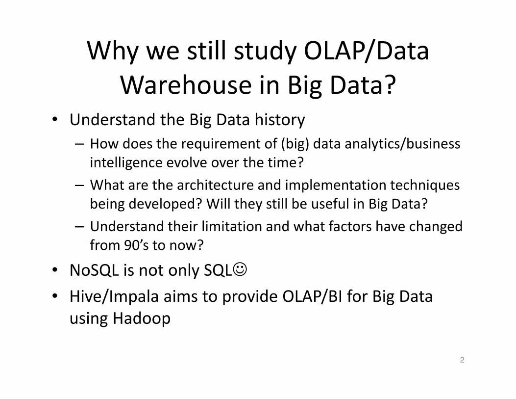
Why we still study OLAP/Data
Warehouse in Big Data?• Understand the Big Data history
– How does the requirement of (big) data analytics/business
intelligence evolve over the time?
– What are the architecture and implementation techniques
being developed? Will they still be useful in Big Data?
– Understand their limitation and what factors have changed
from 90’s to now?
• NoSQL is not only SQL☺
• Hive/Impala aims to provide OLAP/BI for Big Data
using Hadoop
2
Highlights
• OLAP
– Multi-relational Data model
– Operators
– SQL
• Data warehouse (architecture, issues,
optimizations)
• Join Processing
• Column Stores (Optimized for OLAP workload)
3
Let’s get back to the root in 70’s:
Relational Database
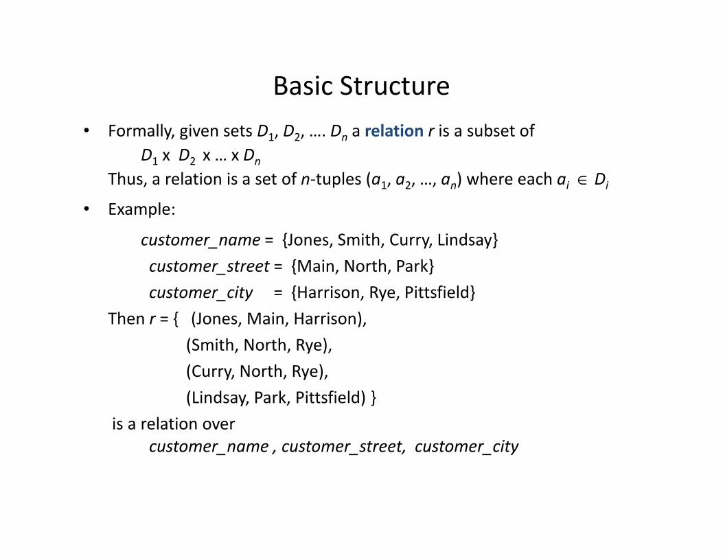
Basic Structure
• Formally, given sets D1, D2, …. Dn a relation r is a subset of
D1 x D2 x … x Dn
Thus, a relation is a set of n-tuples (a1, a2, …, an) where each ai ∈ Di
• Example:
customer_name = {Jones, Smith, Curry, Lindsay}
customer_street = {Main, North, Park}
customer_city = {Harrison, Rye, Pittsfield}
Then r = { (Jones, Main, Harrison),
(Smith, North, Rye),
(Curry, North, Rye),
(Lindsay, Park, Pittsfield) }
is a relation over
customer_name , customer_street, customer_city
Relation Schema
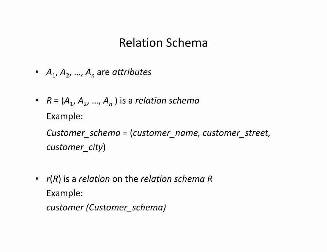
• A1, A2, …, An are attributes
• R = (A1, A2, …, An ) is a relation schema
Example:
Customer_schema = (customer_name, customer_street,
customer_city)
• r(R) is a relation on the relation schema R
Example:
customer (Customer_schema)
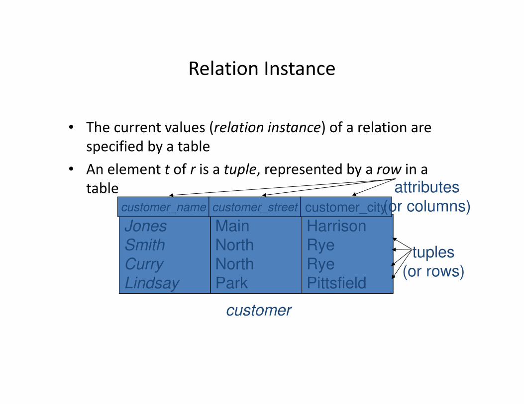
Relation Instance
• The current values (relation instance) of a relation are
specified by a table
• An element t of r is a tuple, represented by a row in a
table
Jones
Smith
Curry
Lindsay
customer_name
Main
North
North
Park
customer_street
Harrison
Rye
Rye
Pittsfield
customer_city
customer
attributes
(or columns)
tuples
(or rows)
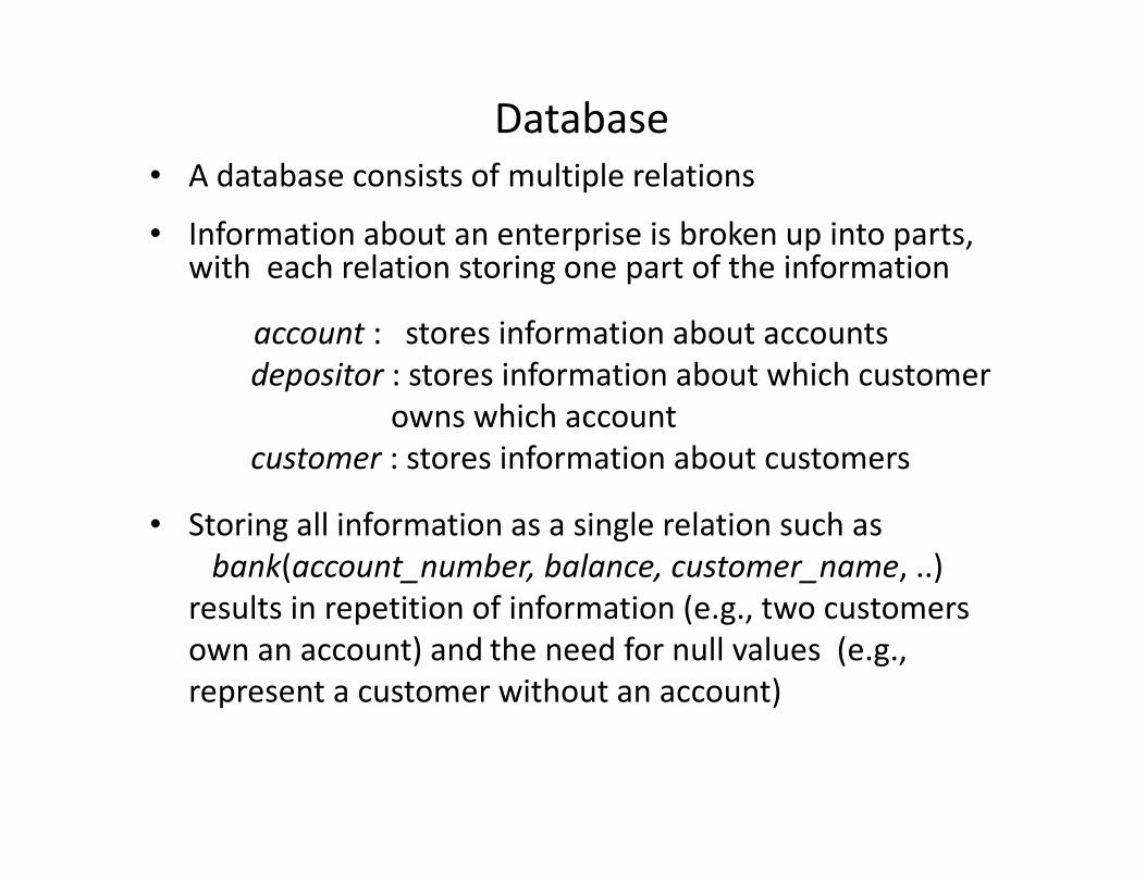
Database
• A database consists of multiple relations
• Information about an enterprise is broken up into parts, with each relation storing one part of the information
account : stores information about accounts
depositor : stores information about which customer
owns which account
customer : stores information about customers
• Storing all information as a single relation such as
bank(account_number, balance, customer_name, ..)
results in repetition of information (e.g., two customers
own an account) and the need for null values (e.g.,
represent a customer without an account)
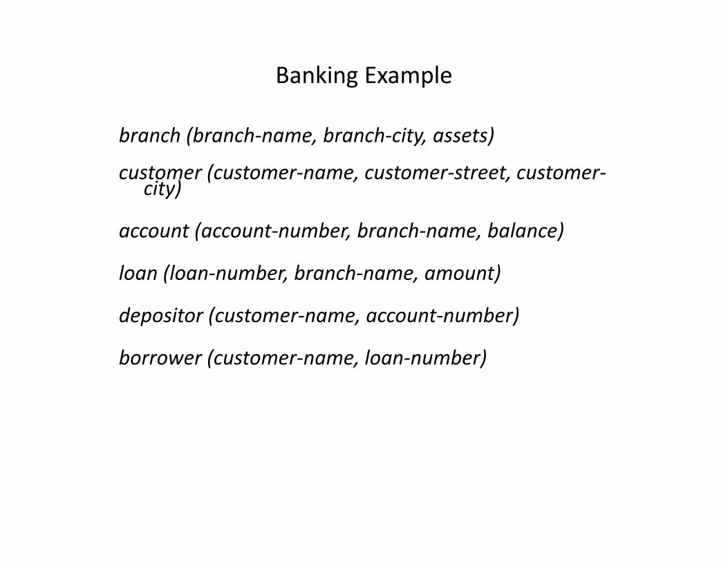
Banking Example
branch (branch-name, branch-city, assets)
customer (customer-name, customer-street, customer-city)
account (account-number, branch-name, balance)
loan (loan-number, branch-name, amount)
depositor (customer-name, account-number)
borrower (customer-name, loan-number)
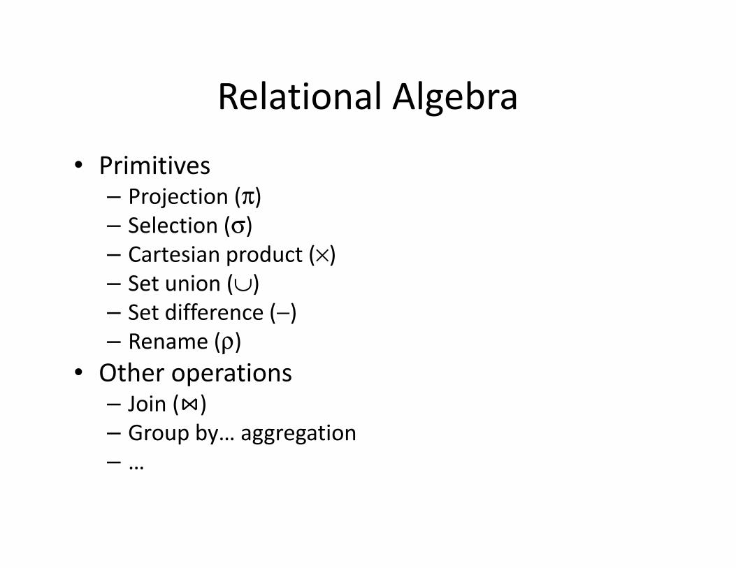
Relational Algebra
• Primitives– Projection (π)
– Selection (σ)
– Cartesian product (×)
– Set union (∪)
– Set difference (−)
– Rename (ρ)
• Other operations– Join (⋈)
– Group by… aggregation
– …
What happens next?
• SQL
• System R (DB2), INGRES, ORACLE, SQL-Server,
Teradata
– B+-Tree (select)
– Transaction Management
– Join algorithm
11
In early 90’s:
OLAP & Data Warehouse
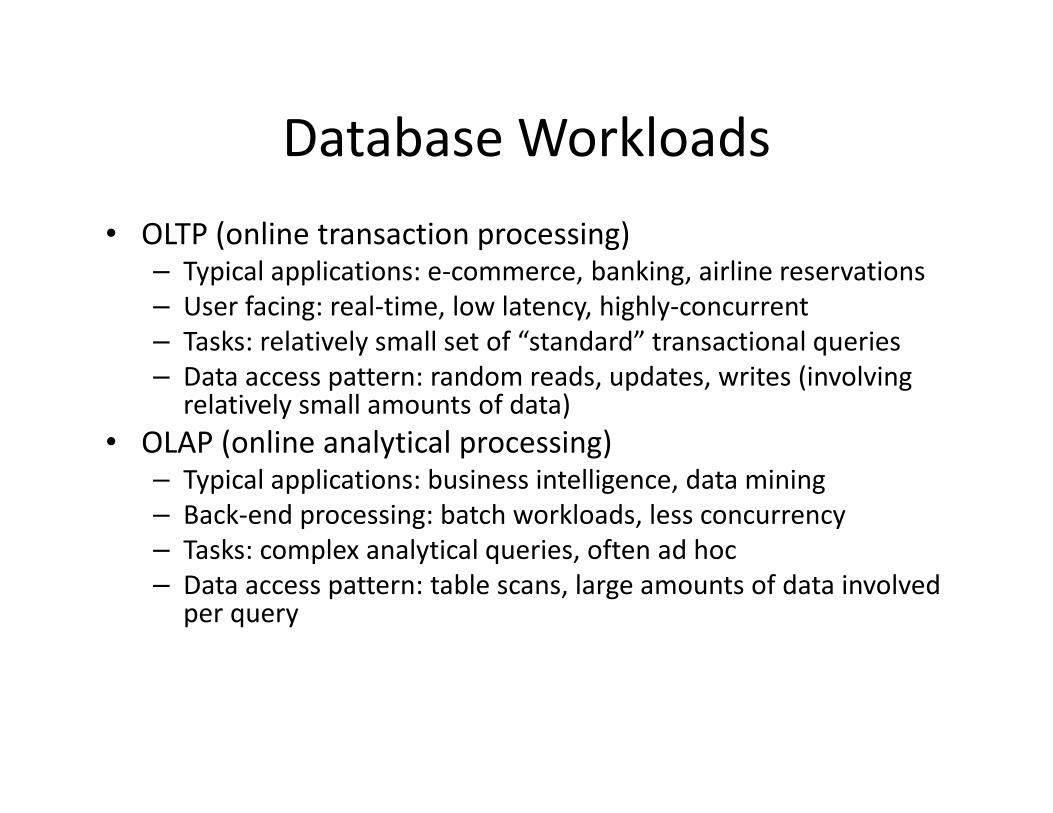
Database Workloads
• OLTP (online transaction processing)– Typical applications: e-commerce, banking, airline reservations
– User facing: real-time, low latency, highly-concurrent
– Tasks: relatively small set of “standard” transactional queries
– Data access pattern: random reads, updates, writes (involving relatively small amounts of data)
• OLAP (online analytical processing)– Typical applications: business intelligence, data mining
– Back-end processing: batch workloads, less concurrency
– Tasks: complex analytical queries, often ad hoc
– Data access pattern: table scans, large amounts of data involved per query
14
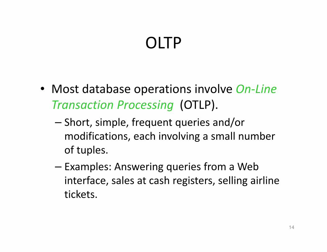
OLTP
• Most database operations involve On-Line
Transaction Processing (OTLP).
– Short, simple, frequent queries and/or
modifications, each involving a small number
of tuples.
– Examples: Answering queries from a Web
interface, sales at cash registers, selling airline
tickets.
15
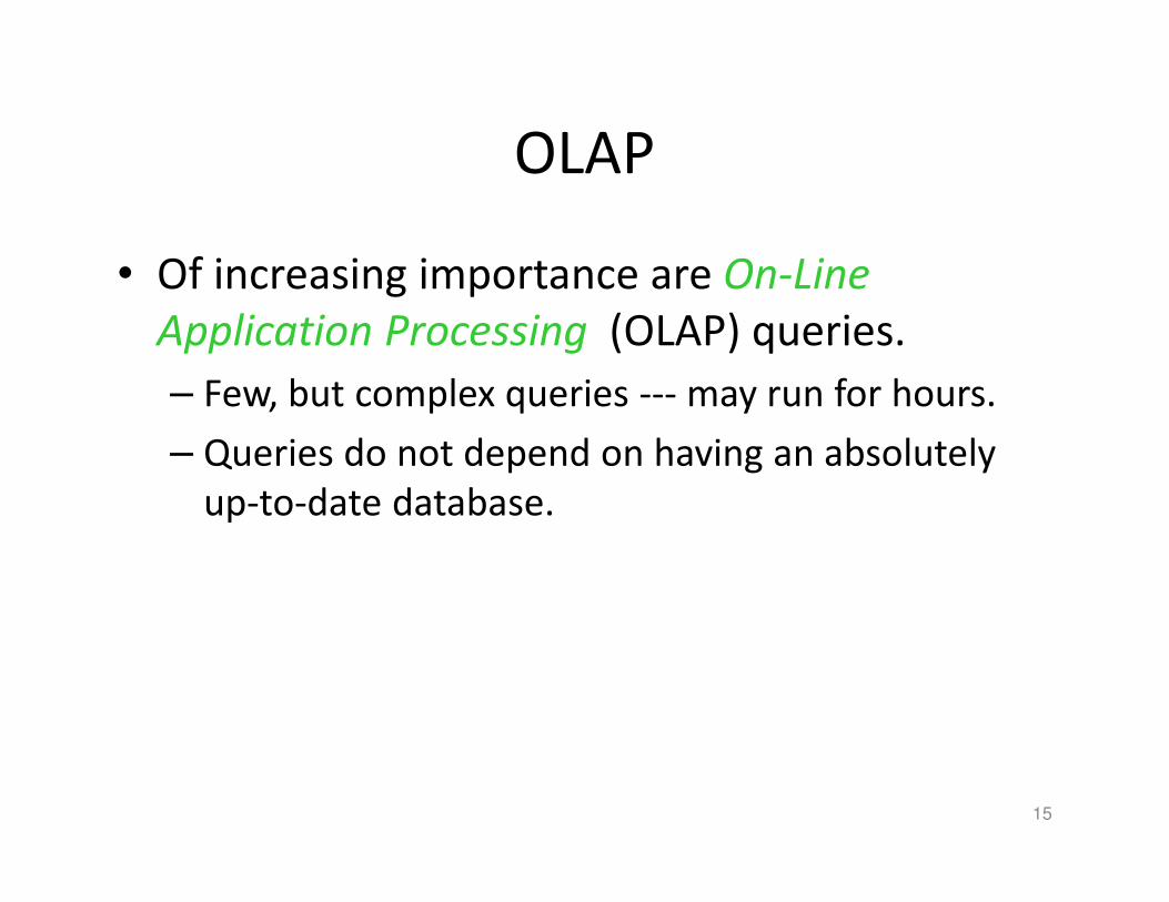
OLAP
• Of increasing importance are On-Line
Application Processing (OLAP) queries.
– Few, but complex queries --- may run for hours.
– Queries do not depend on having an absolutely
up-to-date database.
16
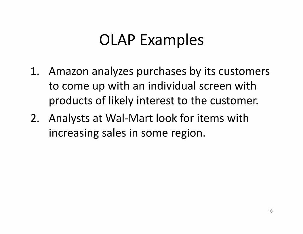
OLAP Examples
1. Amazon analyzes purchases by its customers
to come up with an individual screen with
products of likely interest to the customer.
2. Analysts at Wal-Mart look for items with
increasing sales in some region.
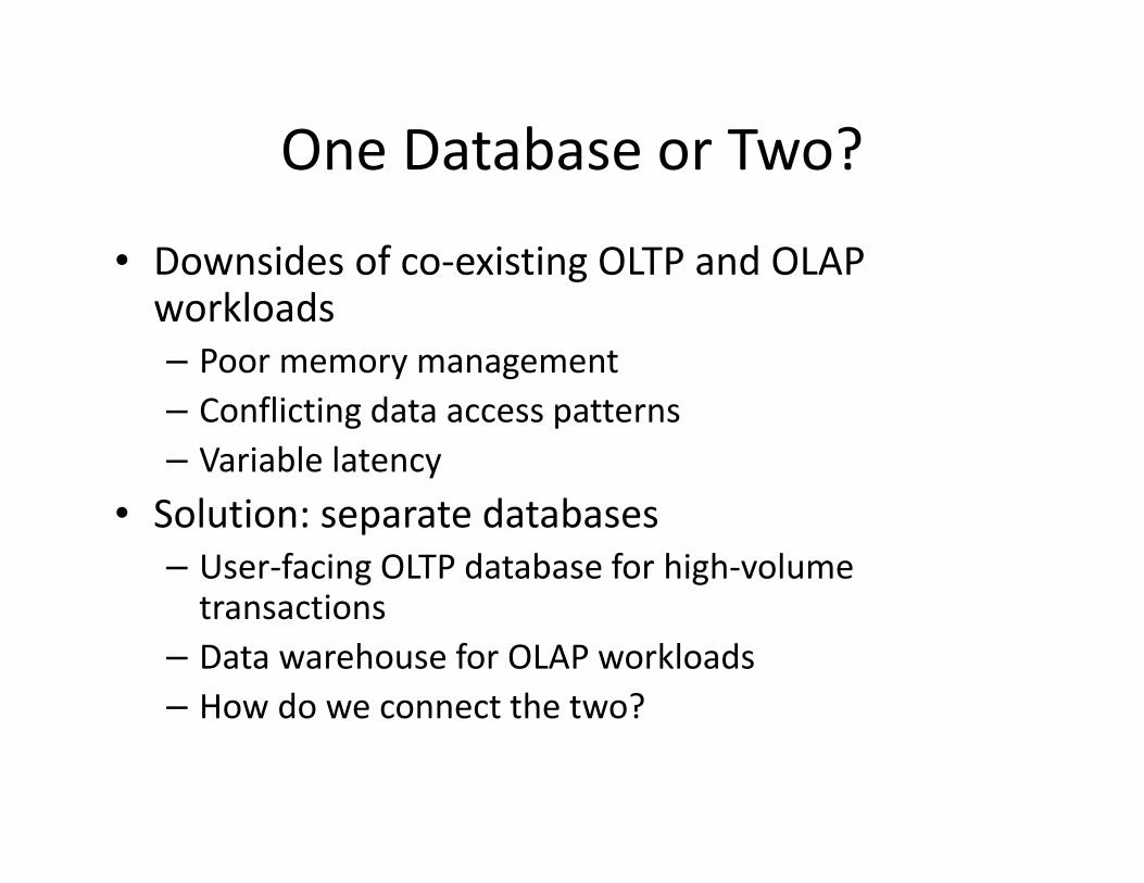
One Database or Two?
• Downsides of co-existing OLTP and OLAP workloads
– Poor memory management
– Conflicting data access patterns
– Variable latency
• Solution: separate databases
– User-facing OLTP database for high-volume transactions
– Data warehouse for OLAP workloads
– How do we connect the two?
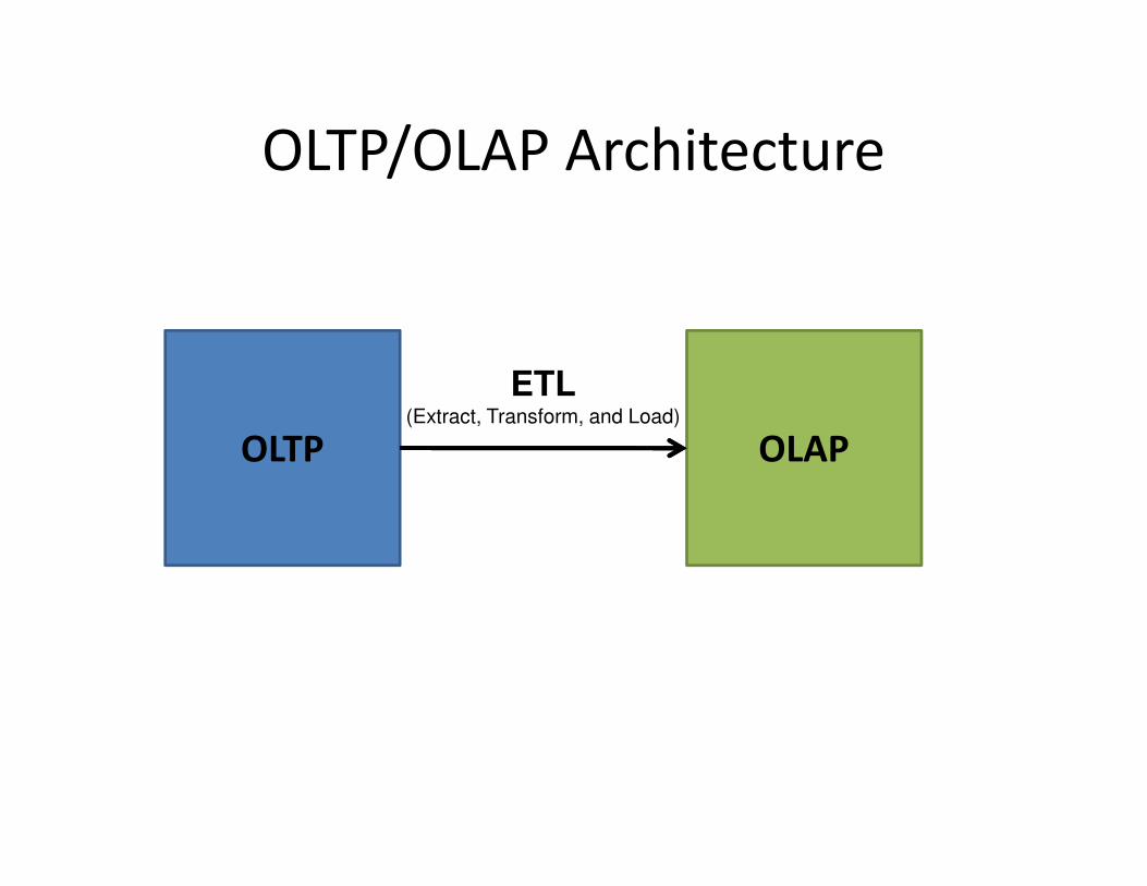
OLTP/OLAP Architecture
OLTP OLAP
ETL(Extract, Transform, and Load)
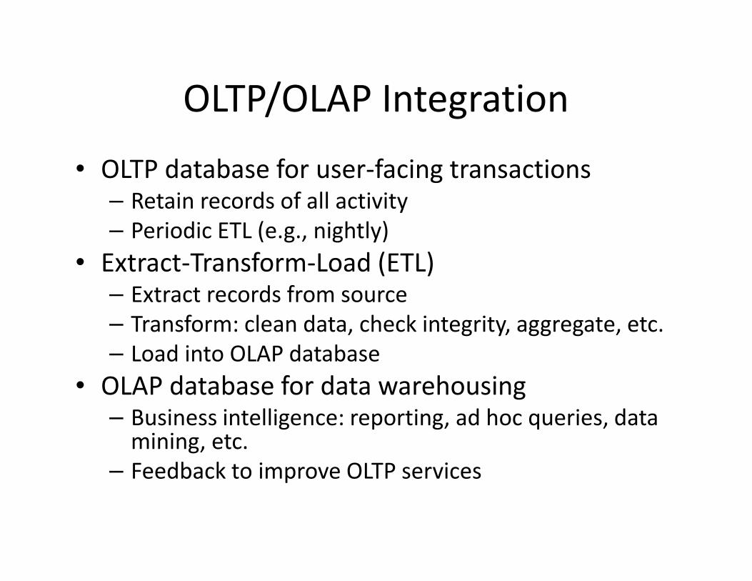
OLTP/OLAP Integration
• OLTP database for user-facing transactions– Retain records of all activity
– Periodic ETL (e.g., nightly)
• Extract-Transform-Load (ETL)– Extract records from source
– Transform: clean data, check integrity, aggregate, etc.
– Load into OLAP database
• OLAP database for data warehousing– Business intelligence: reporting, ad hoc queries, data
mining, etc.
– Feedback to improve OLTP services
20
The Data Warehouse
• The most common form of data integration.
– Copy sources into a single DB (warehouse) and try
to keep it up-to-date.
– Usual method: periodic reconstruction of the
warehouse, perhaps overnight.
– Frequently essential for analytic queries.
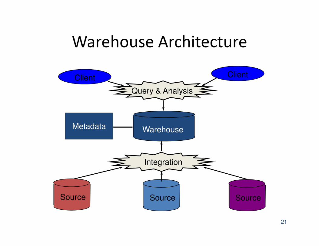
Warehouse Architecture
21
Client Client
Warehouse
Source Source Source
Query & Analysis
Integration
Metadata
22
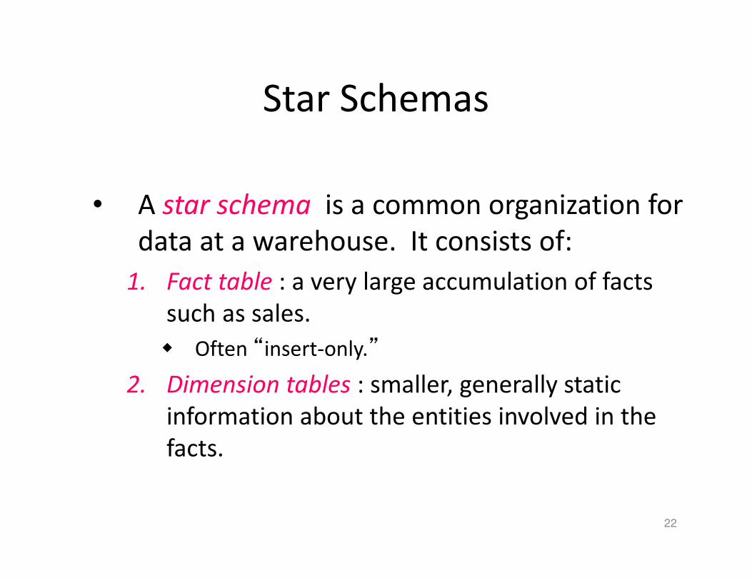
Star Schemas
• A star schema is a common organization for
data at a warehouse. It consists of:
1. Fact table : a very large accumulation of facts
such as sales.
� Often “insert-only.”
2. Dimension tables : smaller, generally static
information about the entities involved in the
facts.
23
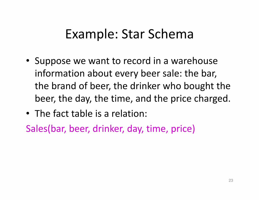
Example: Star Schema
• Suppose we want to record in a warehouse
information about every beer sale: the bar,
the brand of beer, the drinker who bought the
beer, the day, the time, and the price charged.
• The fact table is a relation:
Sales(bar, beer, drinker, day, time, price)
24
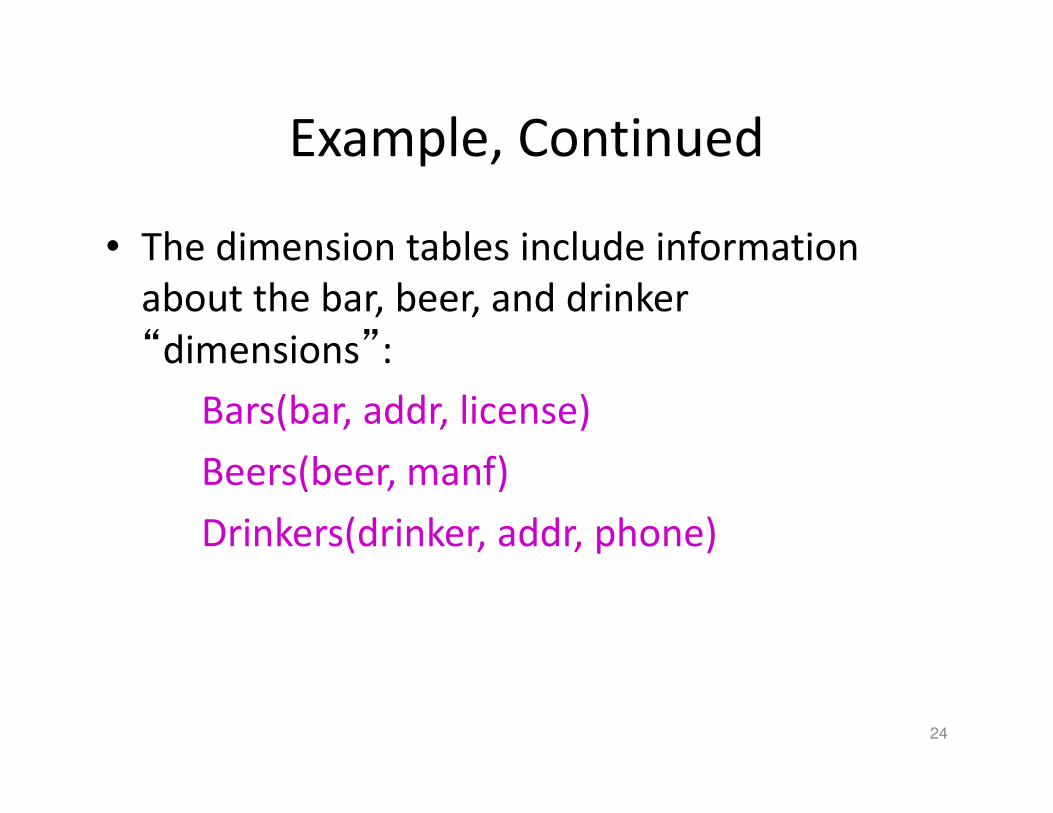
Example, Continued
• The dimension tables include information
about the bar, beer, and drinker
“dimensions”:
Bars(bar, addr, license)
Beers(beer, manf)
Drinkers(drinker, addr, phone)
25
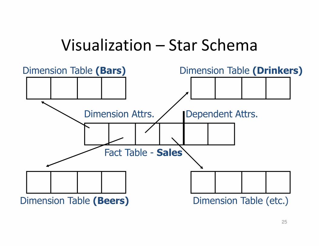
Visualization – Star Schema
Dimension Table (Beers) Dimension Table (etc.)
Dimension Table (Drinkers)Dimension Table (Bars)
Fact Table - Sales
Dimension Attrs. Dependent Attrs.
26
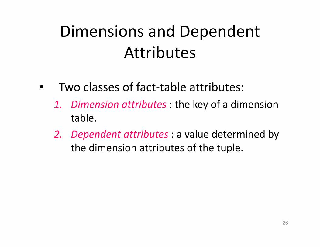
Dimensions and Dependent
Attributes
• Two classes of fact-table attributes:
1. Dimension attributes : the key of a dimension
table.
2. Dependent attributes : a value determined by
the dimension attributes of the tuple.
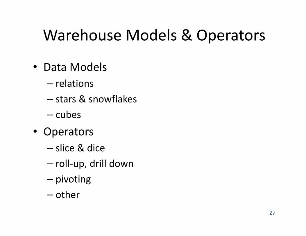
Warehouse Models & Operators
• Data Models
– relations
– stars & snowflakes
– cubes
• Operators
– slice & dice
– roll-up, drill down
– pivoting
– other
27
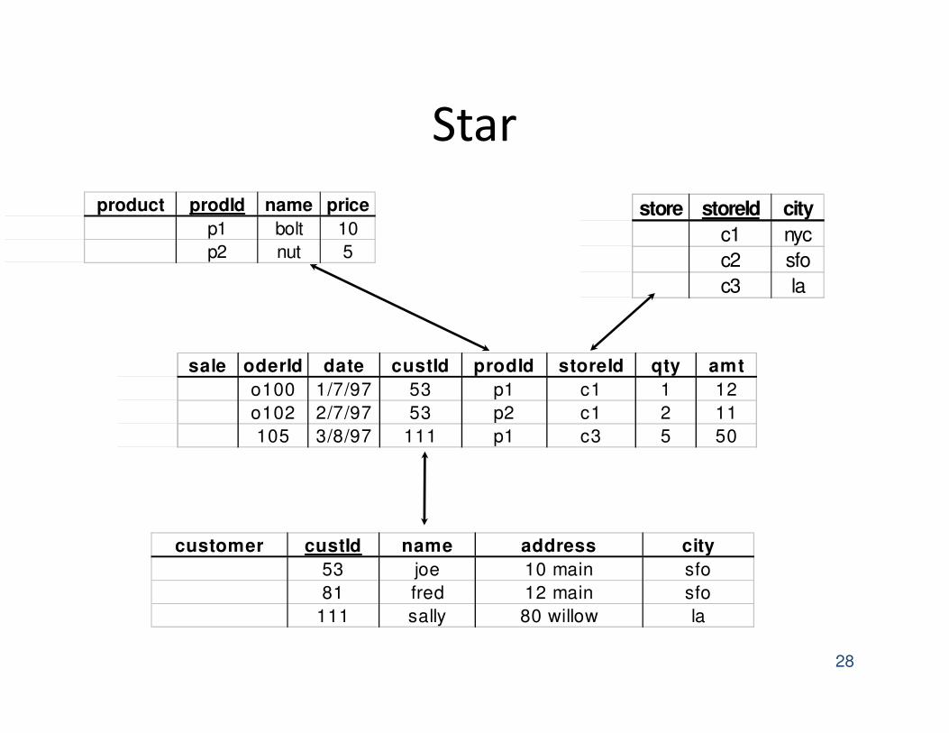
Star
28
customer custId name address city
53 joe 10 main sfo
81 fred 12 main sfo
111 sally 80 willow la
product prodId name price
p1 bolt 10
p2 nut 5
store storeId city
c1 nyc
c2 sfo
c3 la
sale oderId date custId prodId storeId qty amt
o100 1/7/97 53 p1 c1 1 12
o102 2/7/97 53 p2 c1 2 11
105 3/8/97 111 p1 c3 5 50
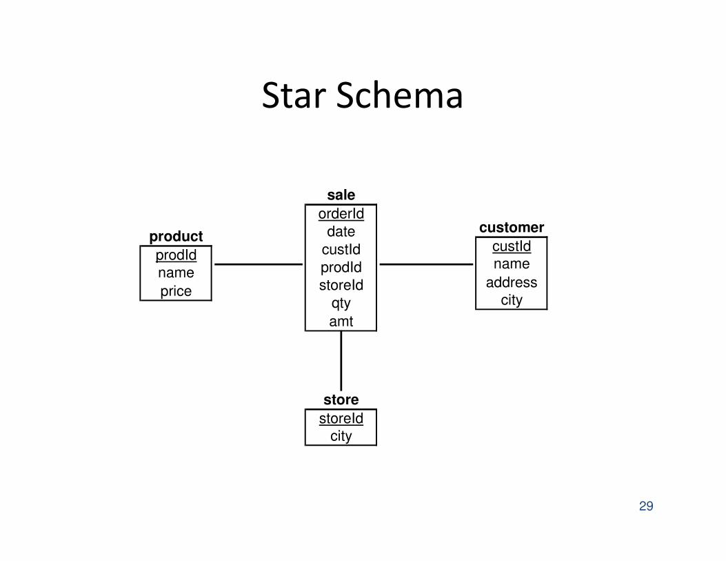
Star Schema
29
sale
orderId
date
custId
prodId
storeId
qty
amt
customer
custId
name
address
city
product
prodId
name
price
store
storeId
city
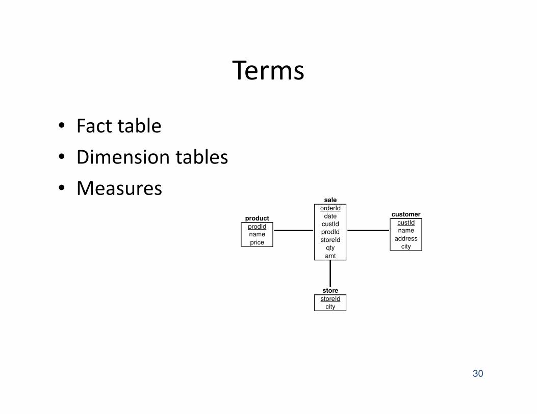
Terms
• Fact table
• Dimension tables
• Measures
30
sale
orderId
date
custId
prodId
storeId
qty
amt
customer
custId
name
address
city
product
prodId
name
price
store
storeId
city
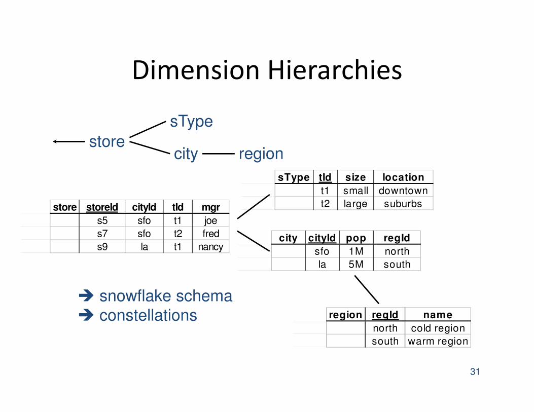
Dimension Hierarchies
31
store storeId cityId tId mgr
s5 sfo t1 joe
s7 sfo t2 fred
s9 la t1 nancycity cityId pop regId
sfo 1M north
la 5M south
region regId name
north cold region
south warm region
sType tId size location
t1 small downtown
t2 large suburbs
store
sType
city region
� snowflake schema
� constellations
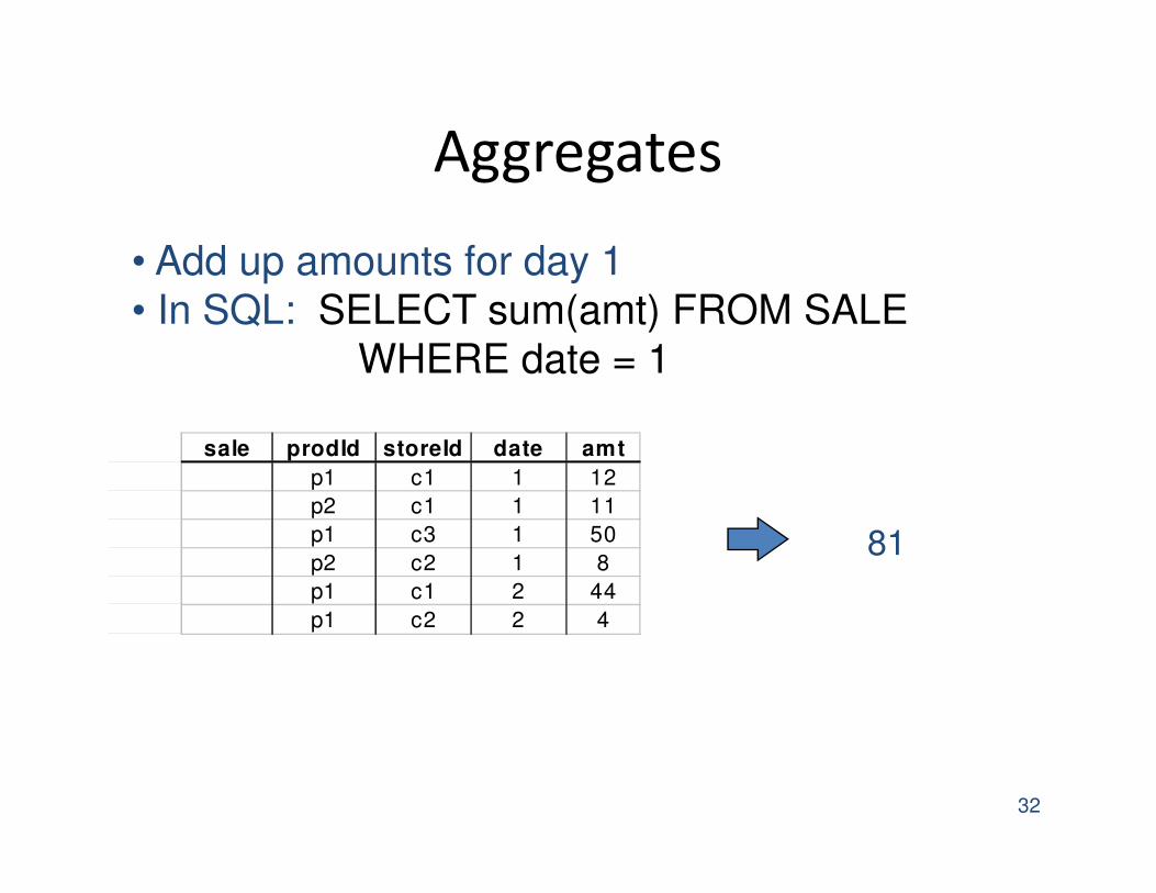
Aggregates
32
sale prodId storeId date amt
p1 c1 1 12
p2 c1 1 11
p1 c3 1 50
p2 c2 1 8
p1 c1 2 44
p1 c2 2 4
• Add up amounts for day 1
• In SQL: SELECT sum(amt) FROM SALE
WHERE date = 1
81
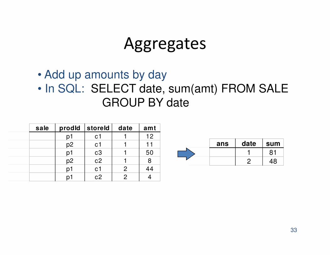
Aggregates
33
sale prodId storeId date amt
p1 c1 1 12
p2 c1 1 11
p1 c3 1 50
p2 c2 1 8
p1 c1 2 44
p1 c2 2 4
• Add up amounts by day
• In SQL: SELECT date, sum(amt) FROM SALE
GROUP BY date
ans date sum
1 81
2 48
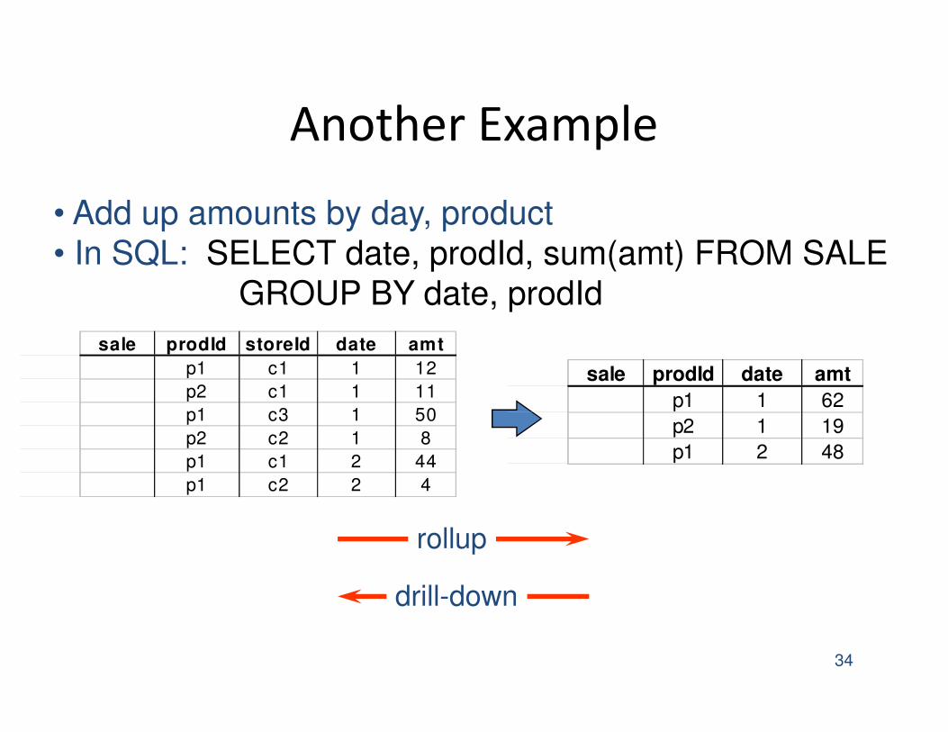
Another Example
34
sale prodId storeId date amt
p1 c1 1 12
p2 c1 1 11
p1 c3 1 50
p2 c2 1 8
p1 c1 2 44
p1 c2 2 4
• Add up amounts by day, product
• In SQL: SELECT date, prodId, sum(amt) FROM SALE
GROUP BY date, prodId
sale prodId date amt
p1 1 62
p2 1 19
p1 2 48
drill-down
rollup
ROLAP vs. MOLAP
• ROLAP:
Relational On-Line Analytical Processing
• MOLAP:
Multi-Dimensional On-Line Analytical
Processing
35
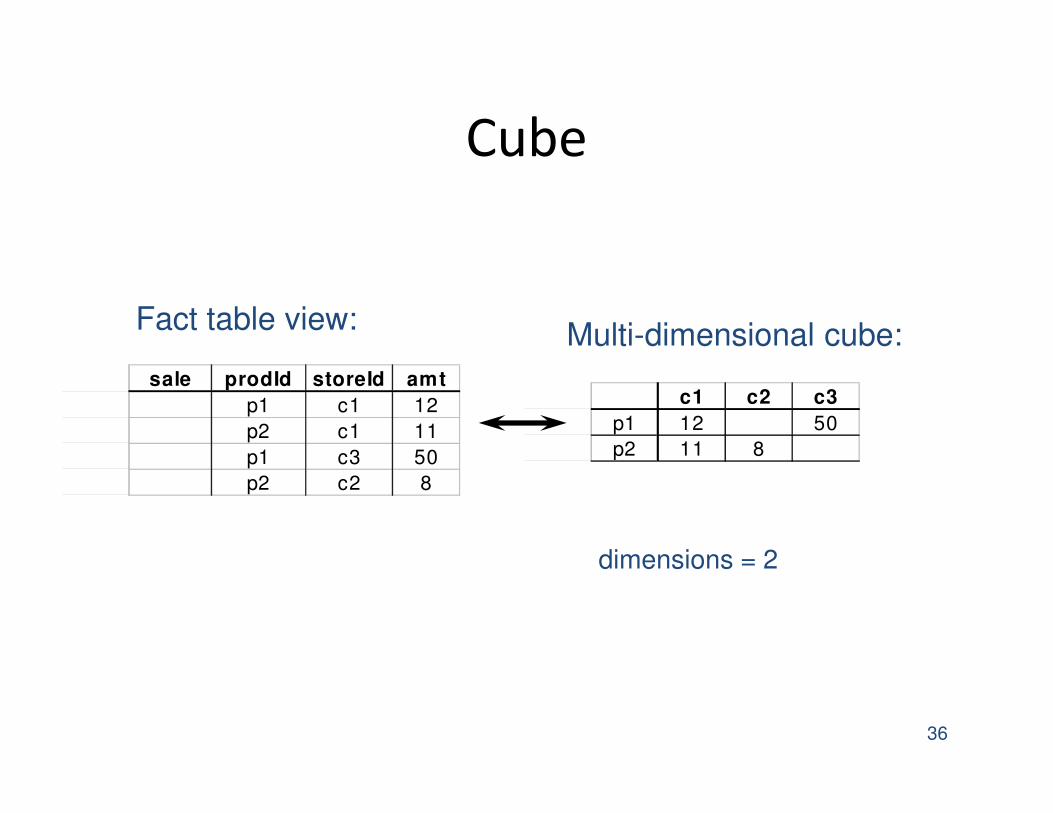
Cube
36
sale prodId storeId amt
p1 c1 12
p2 c1 11
p1 c3 50
p2 c2 8
c1 c2 c3
p1 12 50
p2 11 8
Fact table view:Multi-dimensional cube:
dimensions = 2
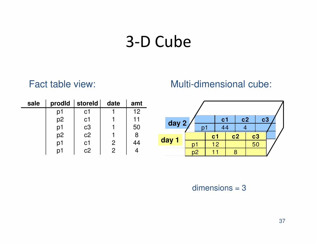
3-D Cube
37
sale prodId storeId date amt
p1 c1 1 12
p2 c1 1 11
p1 c3 1 50
p2 c2 1 8
p1 c1 2 44
p1 c2 2 4
day 2c1 c2 c3
p1 44 4
p2 c1 c2 c3
p1 12 50
p2 11 8
day 1
dimensions = 3
Multi-dimensional cube:Fact table view:
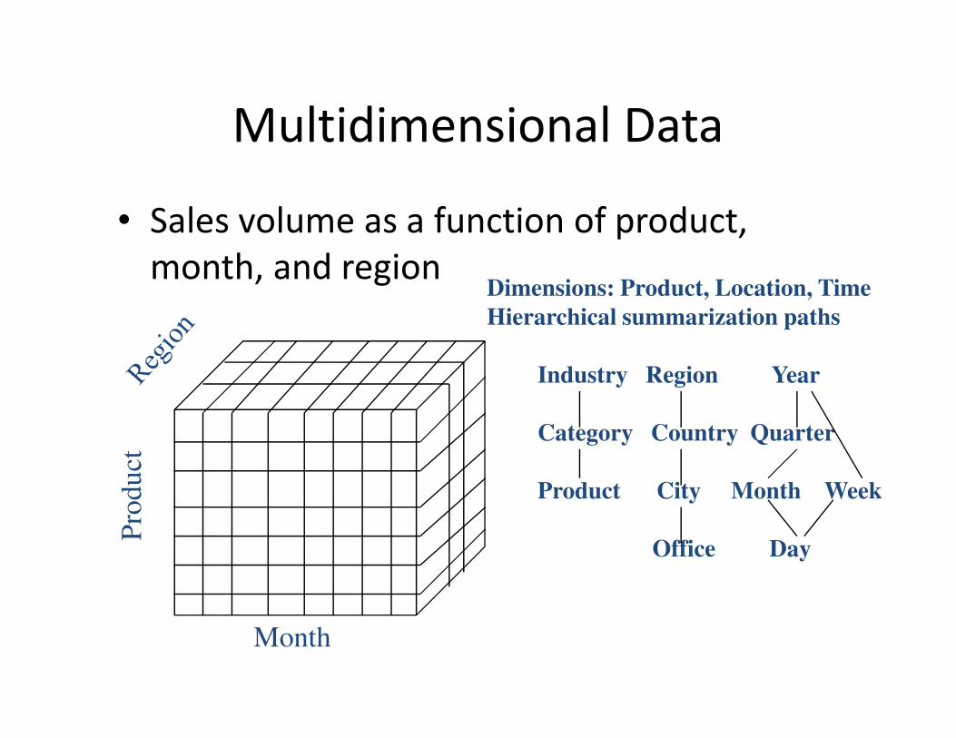
Multidimensional Data
• Sales volume as a function of product,
month, and region
Pro
duct
Month
Dimensions: Product, Location, Time
Hierarchical summarization paths
Industry Region Year
Category Country Quarter
Product City Month Week
Office Day
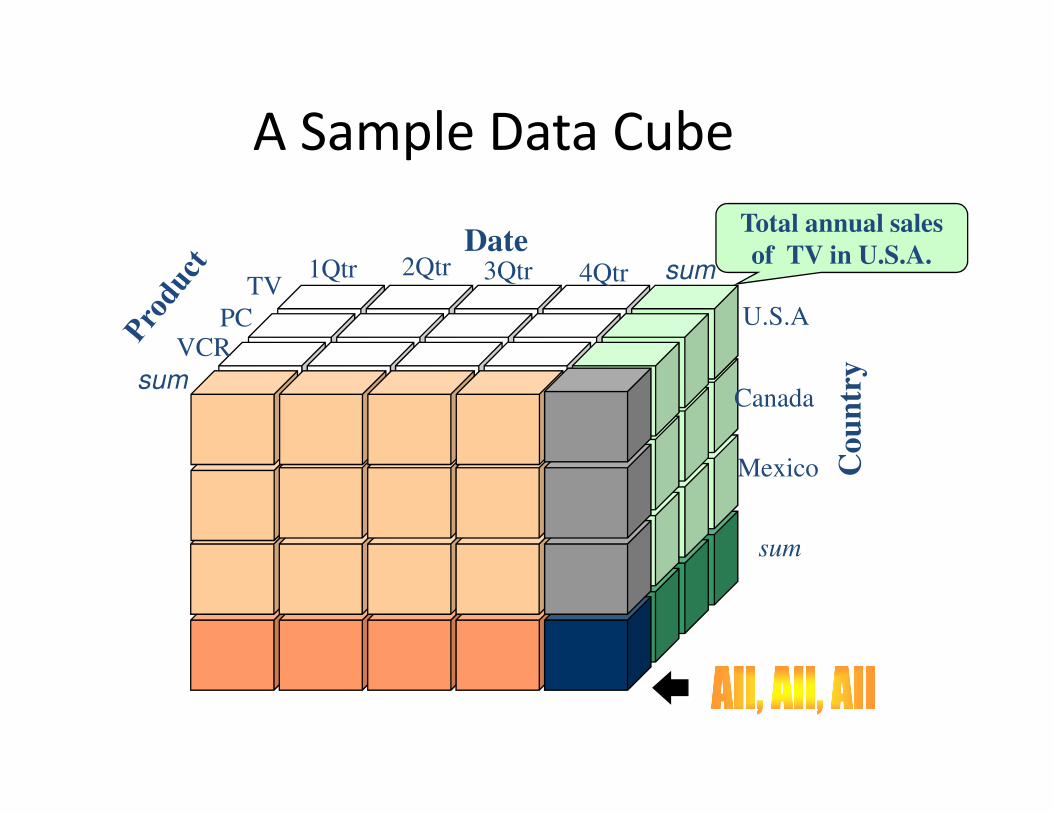
A Sample Data Cube
Total annual sales
of TV in U.S.A.Date
Cou
ntr
ysum
sumTV
VCRPC
1Qtr 2Qtr 3Qtr 4Qtr
U.S.A
Canada
Mexico
sum
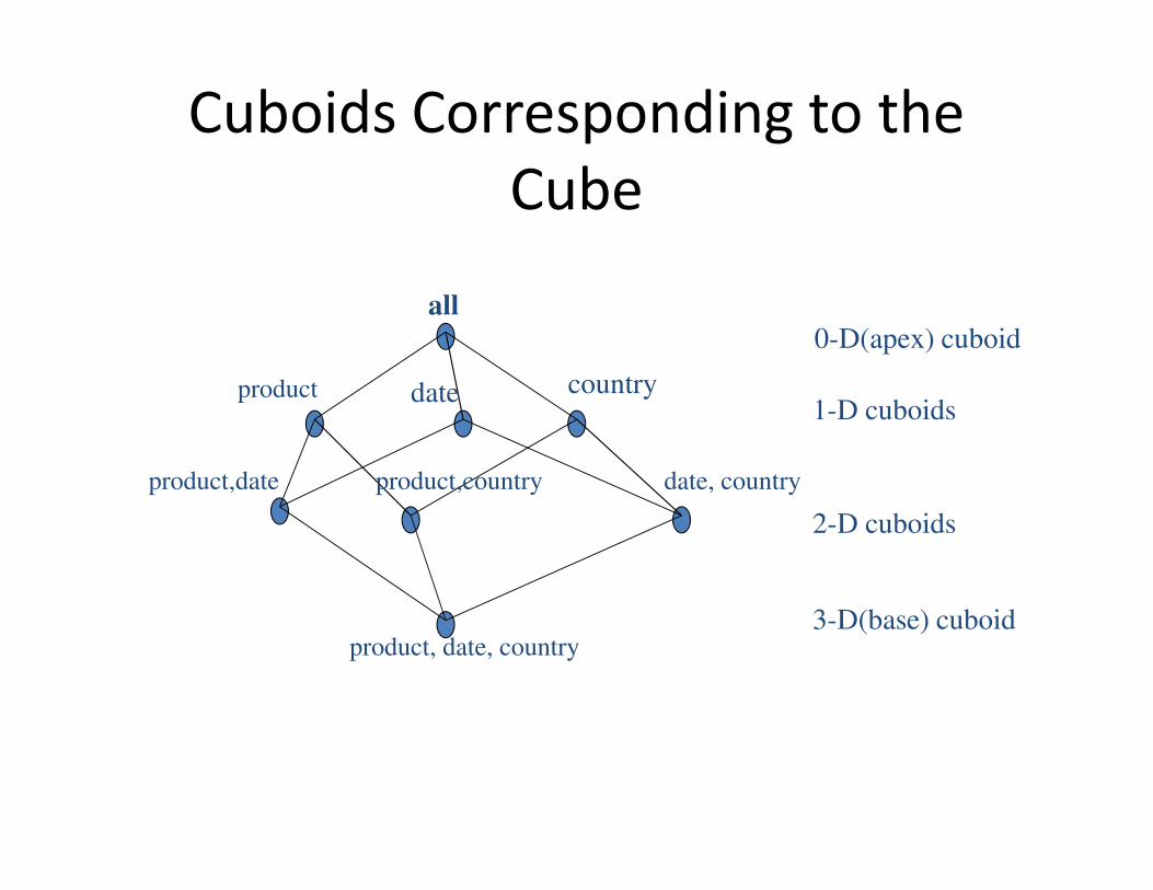
Cuboids Corresponding to the
Cube
all
product date country
product,date product,country date, country
product, date, country
0-D(apex) cuboid
1-D cuboids
2-D cuboids
3-D(base) cuboid
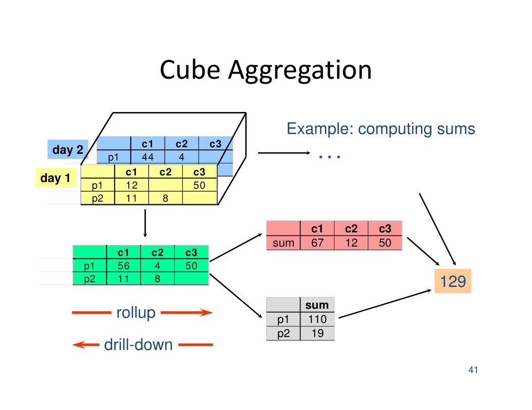
Cube Aggregation
41
day 2c1 c2 c3
p1 44 4
p2 c1 c2 c3
p1 12 50
p2 11 8
day 1
c1 c2 c3
p1 56 4 50
p2 11 8
c1 c2 c3
sum 67 12 50
sum
p1 110
p2 19
129
. . .
drill-down
rollup
Example: computing sums
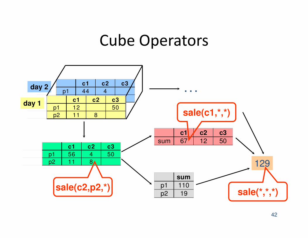
Cube Operators
42
day 2c1 c2 c3
p1 44 4
p2 c1 c2 c3
p1 12 50
p2 11 8
day 1
c1 c2 c3
p1 56 4 50
p2 11 8
c1 c2 c3
sum 67 12 50
sum
p1 110
p2 19
129
. . .
sale(c1,*,*)
sale(*,*,*)sale(c2,p2,*)
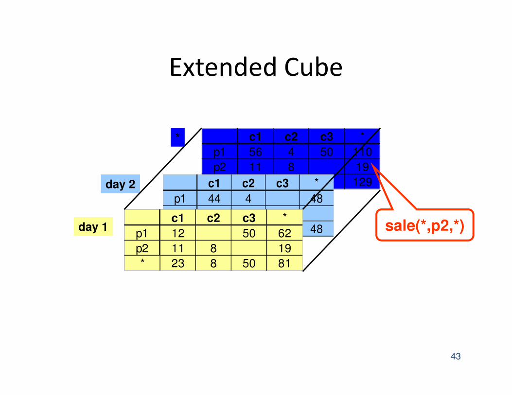
Extended Cube
43
c1 c2 c3 *
p1 56 4 50 110
p2 11 8 19
* 67 12 50 129day 2 c1 c2 c3 *
p1 44 4 48
p2
* 44 4 48c1 c2 c3 *
p1 12 50 62
p2 11 8 19
* 23 8 50 81
day 1
*
sale(*,p2,*)
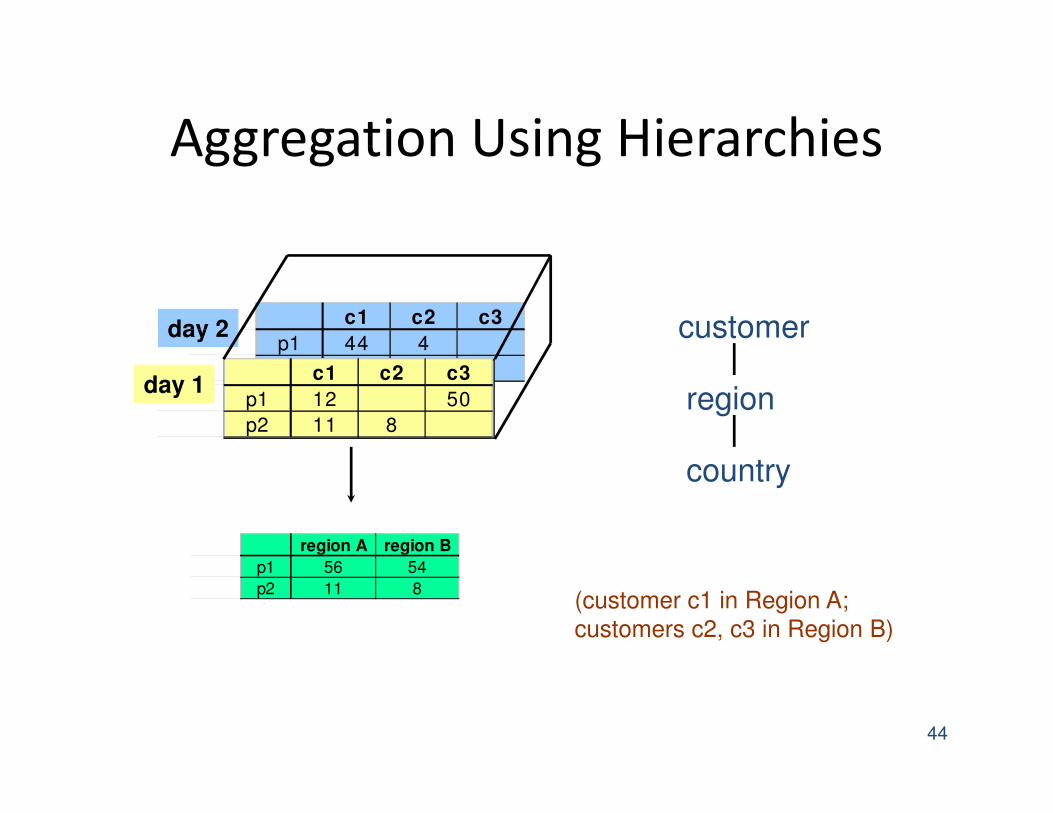
Aggregation Using Hierarchies
44
day 2c1 c2 c3
p1 44 4
p2 c1 c2 c3
p1 12 50
p2 11 8
day 1
region A region B
p1 56 54
p2 11 8
customer
region
country
(customer c1 in Region A;
customers c2, c3 in Region B)
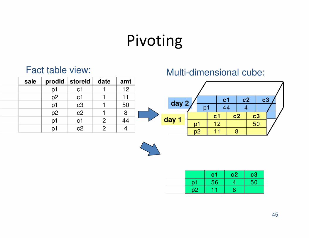
Pivoting
45
sale prodId storeId date amt
p1 c1 1 12
p2 c1 1 11
p1 c3 1 50
p2 c2 1 8
p1 c1 2 44
p1 c2 2 4
day 2c1 c2 c3
p1 44 4
p2 c1 c2 c3
p1 12 50
p2 11 8
day 1
Multi-dimensional cube:Fact table view:
c1 c2 c3
p1 56 4 50
p2 11 8
46
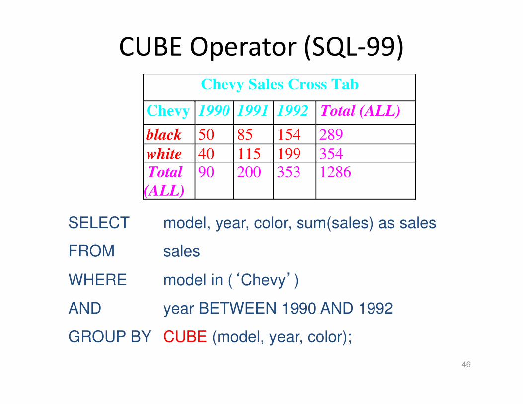
CUBE Operator (SQL-99)
Chevy Sales Cross Tab
Chevy 1990 1991 1992 Total (ALL)
black 50 85 154 289
white 40 115 199 354
Total
(ALL)
90 200 353 1286
SELECT model, year, color, sum(sales) as sales
FROM sales
WHERE model in (‘Chevy’)
AND year BETWEEN 1990 AND 1992
GROUP BY CUBE (model, year, color);
47
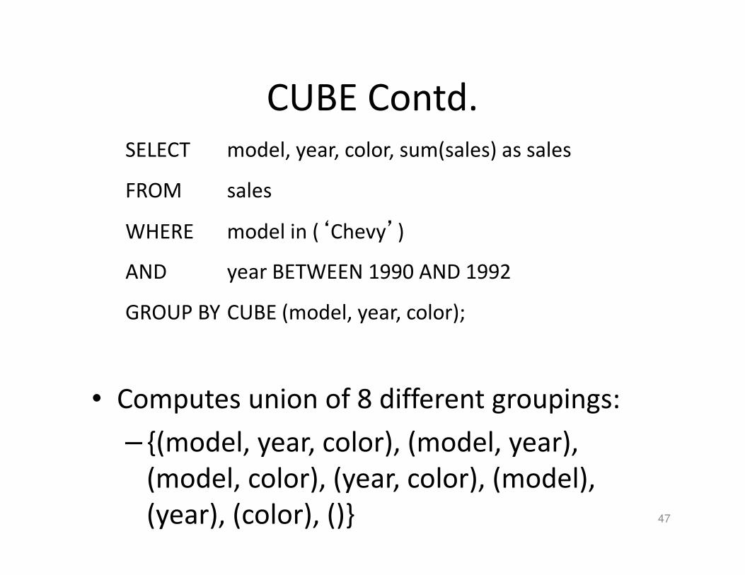
CUBE Contd.
SELECT model, year, color, sum(sales) as sales
FROM sales
WHERE model in (‘Chevy’)
AND year BETWEEN 1990 AND 1992
GROUP BY CUBE (model, year, color);
• Computes union of 8 different groupings:
– {(model, year, color), (model, year),
(model, color), (year, color), (model),
(year), (color), ()}
48
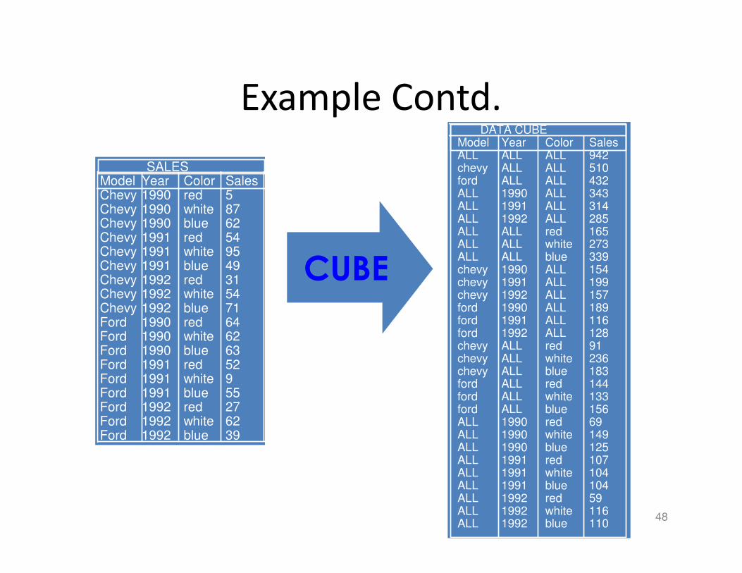
Example Contd.
CUBE
SALES Model Year Color Sales Chevy 1990 red 5 Chevy 1990 white 87 Chevy 1990 blue 62 Chevy 1991 red 54 Chevy 1991 white 95 Chevy 1991 blue 49 Chevy 1992 red 31 Chevy 1992 white 54 Chevy 1992 blue 71 Ford 1990 red 64 Ford 1990 white 62 Ford 1990 blue 63 Ford 1991 red 52 Ford 1991 white 9 Ford 1991 blue 55 Ford 1992 red 27 Ford 1992 white 62 Ford 1992 blue 39
DATA CUBE Model Year Color Sales ALL ALL ALL 942 chevy ALL ALL 510 ford ALL ALL 432 ALL 1990 ALL 343 ALL 1991 ALL 314 ALL 1992 ALL 285 ALL ALL red 165 ALL ALL white 273 ALL ALL blue 339 chevy 1990 ALL 154 chevy 1991 ALL 199 chevy 1992 ALL 157 ford 1990 ALL 189 ford 1991 ALL 116 ford 1992 ALL 128 chevy ALL red 91 chevy ALL white 236 chevy ALL blue 183 ford ALL red 144 ford ALL white 133 ford ALL blue 156 ALL 1990 red 69 ALL 1990 white 149 ALL 1990 blue 125 ALL 1991 red 107 ALL 1991 white 104 ALL 1991 blue 104 ALL 1992 red 59 ALL 1992 white 116 ALL 1992 blue 110
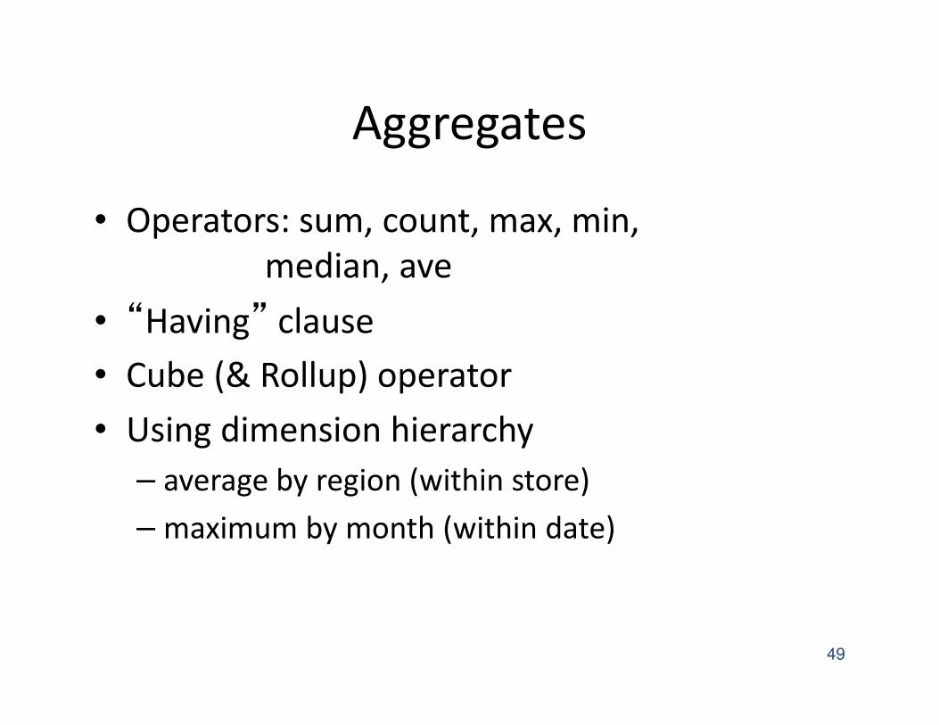
Aggregates
• Operators: sum, count, max, min,
median, ave
• “Having” clause
• Cube (& Rollup) operator
• Using dimension hierarchy
– average by region (within store)
– maximum by month (within date)
49
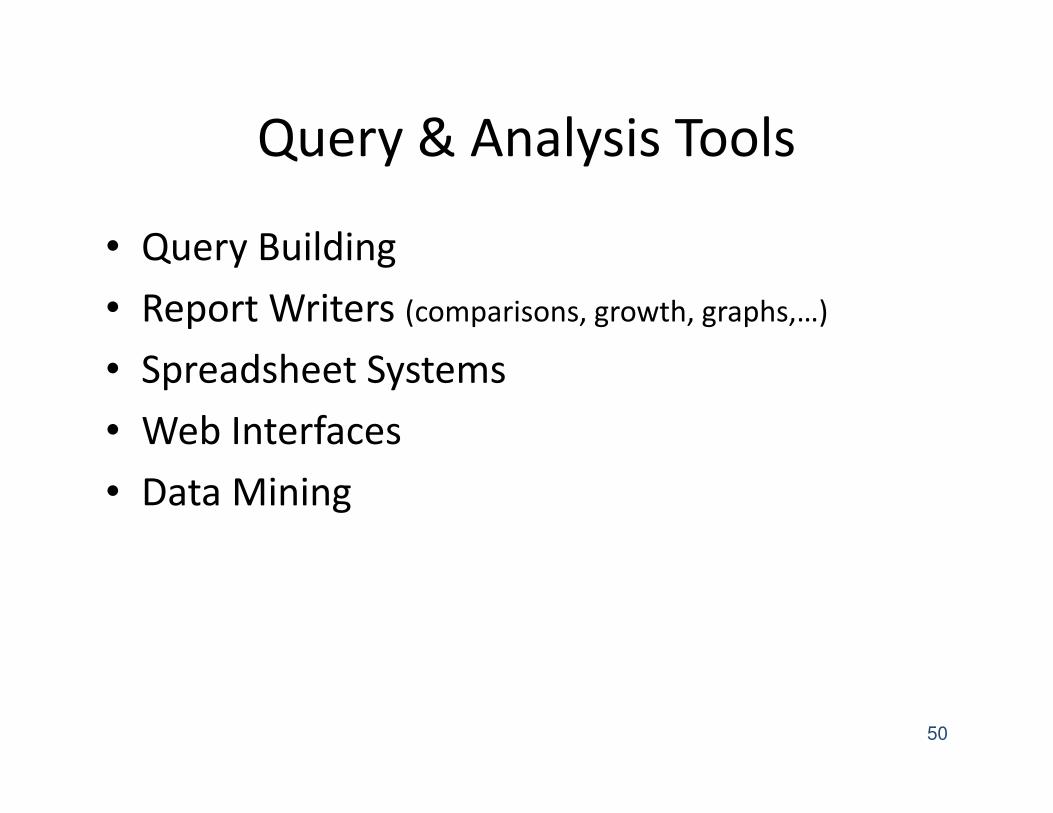
Query & Analysis Tools
• Query Building
• Report Writers (comparisons, growth, graphs,…)
• Spreadsheet Systems
• Web Interfaces
• Data Mining
50
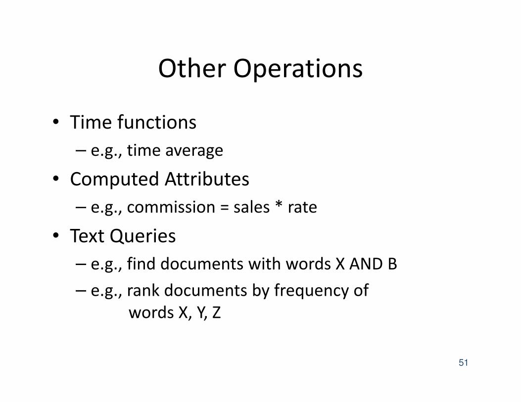
Other Operations
• Time functions
– e.g., time average
• Computed Attributes
– e.g., commission = sales * rate
• Text Queries
– e.g., find documents with words X AND B
– e.g., rank documents by frequency of
words X, Y, Z
51
Data Warehouse Implementation
Implementing a Warehouse
• Monitoring: Sending data from sources
• Integrating: Loading, cleansing,...
• Processing: Query processing, indexing, ...
• Managing: Metadata, Design, ...
53
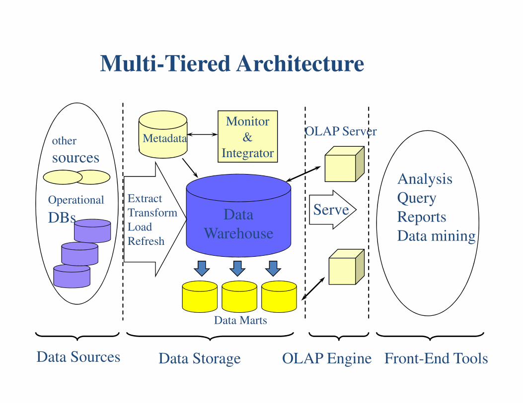
Multi-Tiered Architecture
Data
Warehouse
Extract
Transform
Load
Refresh
OLAP Engine
Analysis
Query
Reports
Data mining
Monitor
&
Integrator
Metadata
Data Sources Front-End Tools
Serve
Data Marts
Operational
DBs
other
sources
Data Storage
OLAP Server
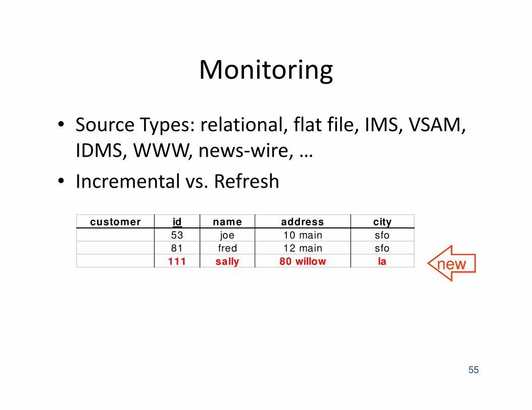
Monitoring
• Source Types: relational, flat file, IMS, VSAM,
IDMS, WWW, news-wire, …
• Incremental vs. Refresh
55
customer id name address city
53 joe 10 main sfo
81 fred 12 main sfo
111 sally 80 willow la new
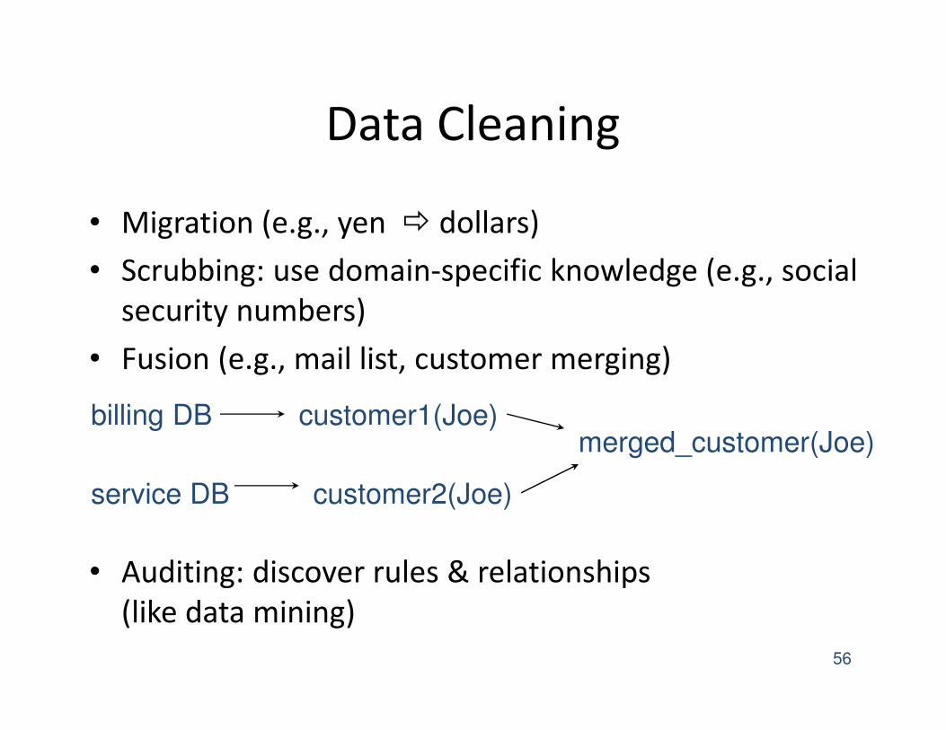
Data Cleaning
• Migration (e.g., yen � dollars)
• Scrubbing: use domain-specific knowledge (e.g., social
security numbers)
• Fusion (e.g., mail list, customer merging)
• Auditing: discover rules & relationships
(like data mining)
56
billing DB
service DB
customer1(Joe)
customer2(Joe)
merged_customer(Joe)
Loading Data
• Incremental vs. refresh
• Off-line vs. on-line
• Frequency of loading
– At night, 1x a week/month, continuously
• Parallel/Partitioned load
57

OLAP Implementation
Derived Data
• Derived Warehouse Data
– indexes
– aggregates
– materialized views (next slide)
• When to update derived data?
• Incremental vs. refresh
59
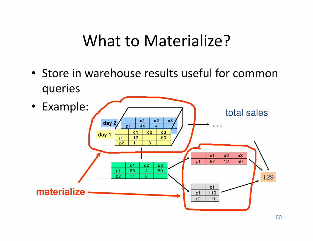
What to Materialize?
• Store in warehouse results useful for common
queries
• Example:
60
day 2c1 c2 c3
p1 44 4
p2 c1 c2 c3
p1 12 50
p2 11 8
day 1
c1 c2 c3
p1 56 4 50
p2 11 8
c1 c2 c3
p1 67 12 50
c1
p1 110
p2 19
129
. . .
total sales
materialize
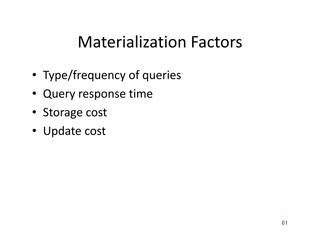
Materialization Factors
• Type/frequency of queries
• Query response time
• Storage cost
• Update cost
61
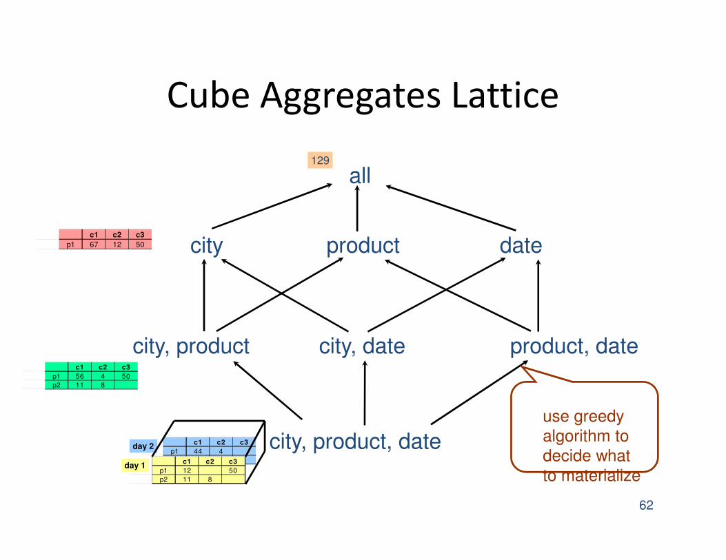
Cube Aggregates Lattice
62
city, product, date
city, product city, date product, date
city product date
all
day 2c1 c2 c3
p1 44 4
p2 c1 c2 c3
p1 12 50
p2 11 8
day 1
c1 c2 c3
p1 56 4 50
p2 11 8
c1 c2 c3
p1 67 12 50
129
use greedy
algorithm to
decide what
to materialize
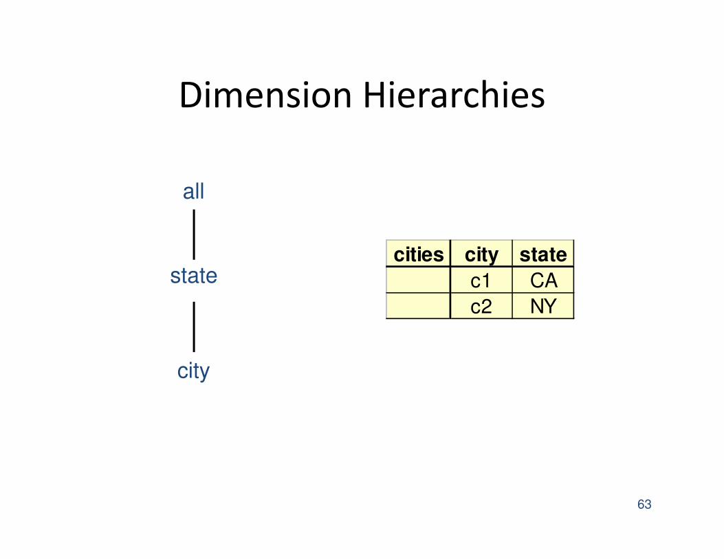
Dimension Hierarchies
63
all
state
city
cities city state
c1 CA
c2 NY
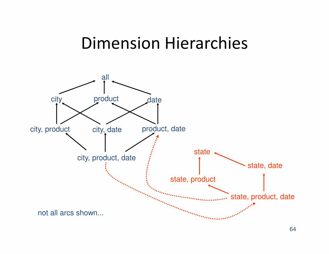
Dimension Hierarchies
64
city, product
city, product, date
city, date product, date
city product date
all
state, product, date
state, date
state, product
state
not all arcs shown...
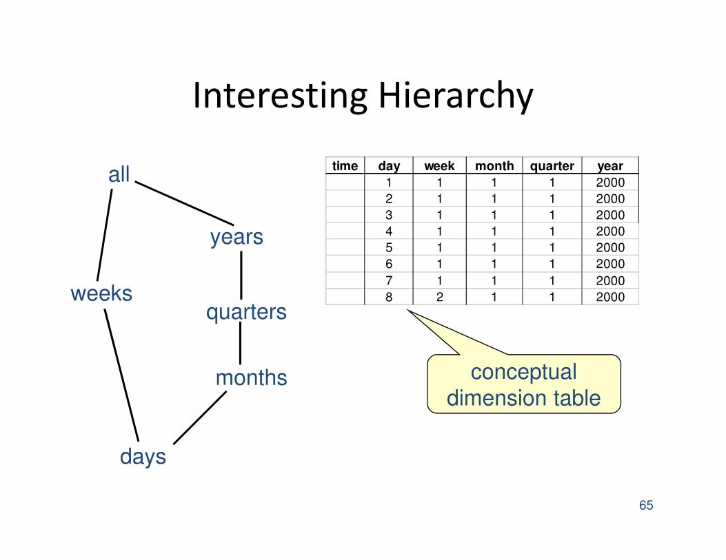
Interesting Hierarchy
65
all
years
quarters
months
days
weeks
time day week month quarter year
1 1 1 1 2000
2 1 1 1 2000
3 1 1 1 2000
4 1 1 1 2000
5 1 1 1 2000
6 1 1 1 2000
7 1 1 1 2000
8 2 1 1 2000
conceptual
dimension table
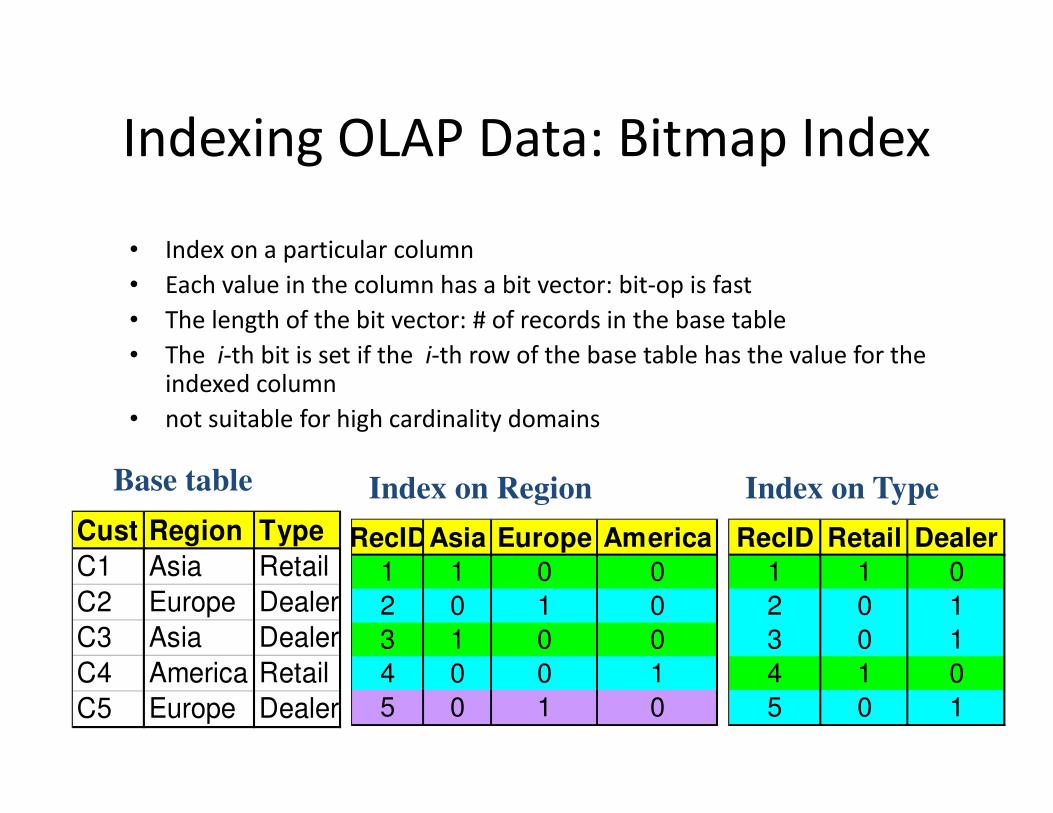
Indexing OLAP Data: Bitmap Index
• Index on a particular column
• Each value in the column has a bit vector: bit-op is fast
• The length of the bit vector: # of records in the base table
• The i-th bit is set if the i-th row of the base table has the value for the indexed column
• not suitable for high cardinality domains
Cust Region Type
C1 Asia Retail
C2 Europe Dealer
C3 Asia Dealer
C4 America Retail
C5 Europe Dealer
RecID Retail Dealer
1 1 0
2 0 1
3 0 1
4 1 0
5 0 1
RecIDAsia Europe America
1 1 0 0
2 0 1 0
3 1 0 0
4 0 0 1
5 0 1 0
Base table Index on Region Index on Type

Join Processing
Join
• How does DBMS join two tables?
• Sorting is one way...
• Database must choose best way for each
query
Schema for Examples
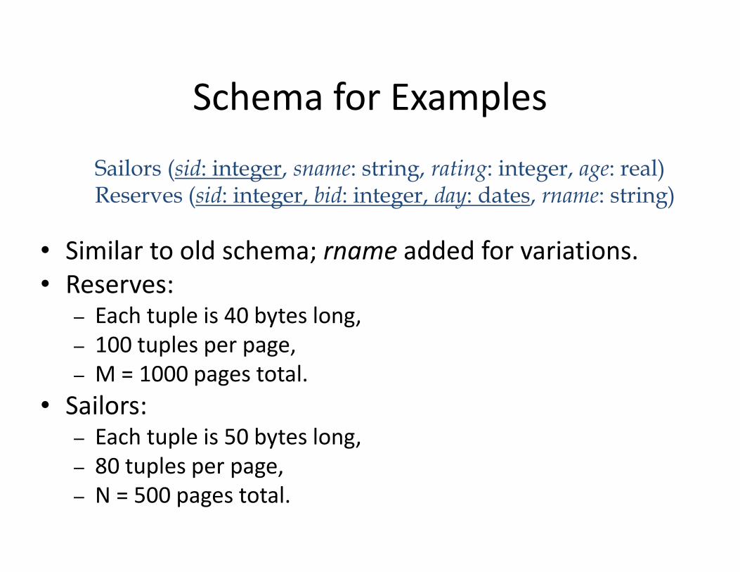
• Similar to old schema; rname added for variations.
• Reserves:– Each tuple is 40 bytes long,
– 100 tuples per page,
– M = 1000 pages total.
• Sailors:– Each tuple is 50 bytes long,
– 80 tuples per page,
– N = 500 pages total.
Sailors (sid: integer, sname: string, rating: integer, age: real)Reserves (sid: integer, bid: integer, day: dates, rname: string)
Equality Joins With One Join Column
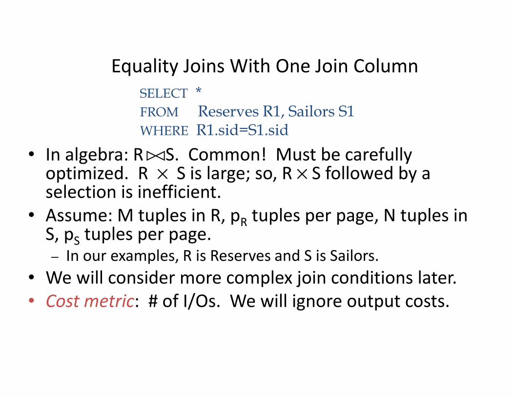
• In algebra: R S. Common! Must be carefully optimized. R × S is large; so, R × S followed by a selection is inefficient.
• Assume: M tuples in R, pR tuples per page, N tuples in S, pS tuples per page.– In our examples, R is Reserves and S is Sailors.
• We will consider more complex join conditions later.
• Cost metric: # of I/Os. We will ignore output costs.
SELECT *FROM Reserves R1, Sailors S1WHERE R1.sid=S1.sid
><
Simple Nested Loops Join
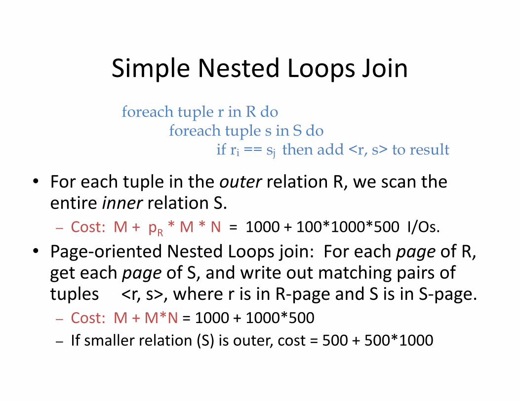
• For each tuple in the outer relation R, we scan the entire inner relation S.
– Cost: M + pR * M * N = 1000 + 100*1000*500 I/Os.
• Page-oriented Nested Loops join: For each page of R, get each page of S, and write out matching pairs of tuples <r, s>, where r is in R-page and S is in S-page.
– Cost: M + M*N = 1000 + 1000*500
– If smaller relation (S) is outer, cost = 500 + 500*1000
foreach tuple r in R doforeach tuple s in S do
if ri == sj then add <r, s> to result
Block Nested Loops Join
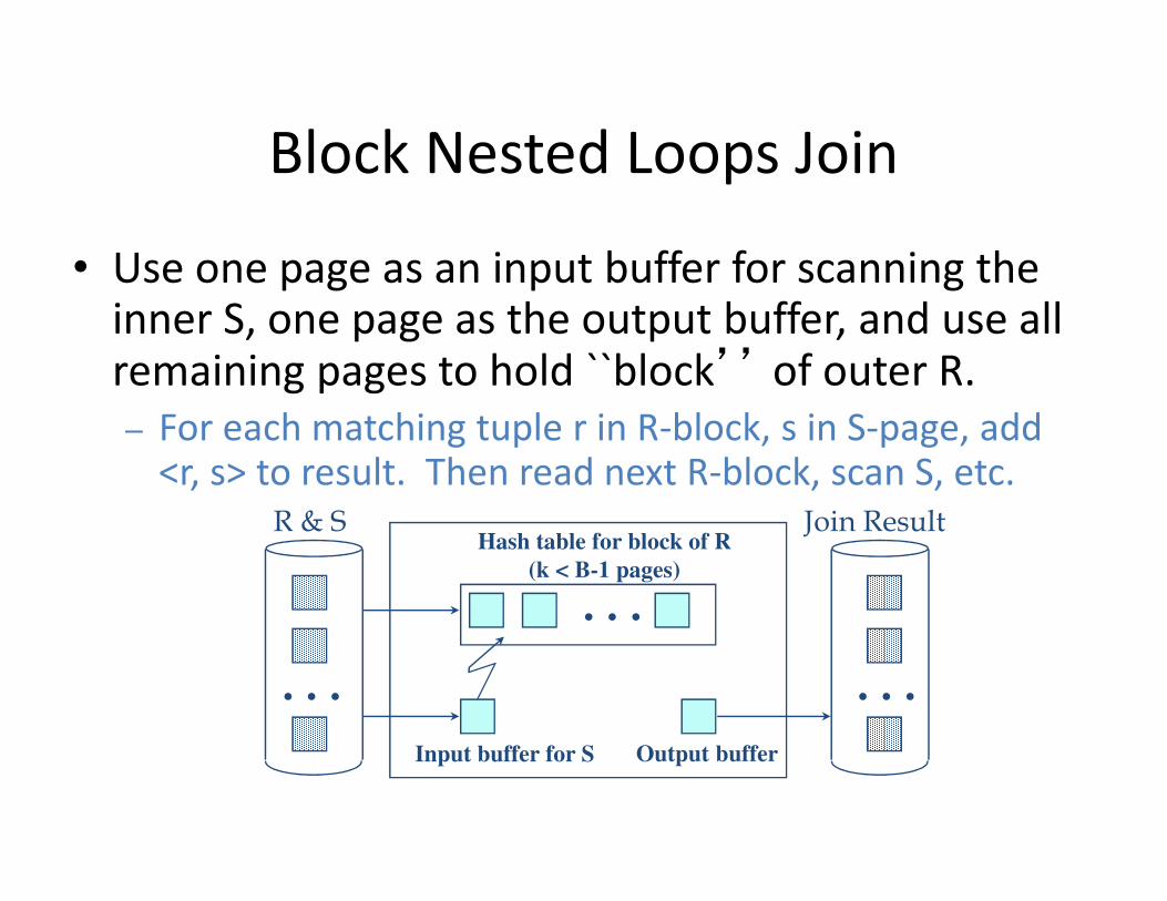
• Use one page as an input buffer for scanning the inner S, one page as the output buffer, and use all remaining pages to hold ``block’’ of outer R.
– For each matching tuple r in R-block, s in S-page, add <r, s> to result. Then read next R-block, scan S, etc.
. . .
. . .
R & SHash table for block of R
(k < B-1 pages)
Input buffer for S Output buffer
. . .
Join Result
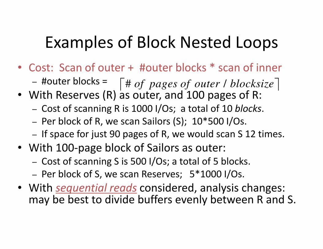
Examples of Block Nested Loops
• Cost: Scan of outer + #outer blocks * scan of inner– #outer blocks =
• With Reserves (R) as outer, and 100 pages of R:– Cost of scanning R is 1000 I/Os; a total of 10 blocks.
– Per block of R, we scan Sailors (S); 10*500 I/Os.
– If space for just 90 pages of R, we would scan S 12 times.
• With 100-page block of Sailors as outer:– Cost of scanning S is 500 I/Os; a total of 5 blocks.
– Per block of S, we scan Reserves; 5*1000 I/Os.
• With sequential reads considered, analysis changes: may be best to divide buffers evenly between R and S.
# /of pages of outer blocksize
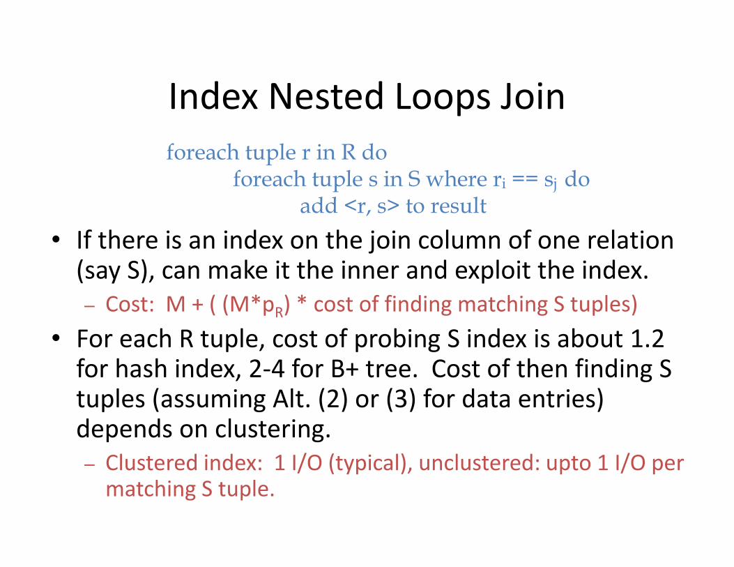
Index Nested Loops Join
• If there is an index on the join column of one relation (say S), can make it the inner and exploit the index.
– Cost: M + ( (M*pR) * cost of finding matching S tuples)
• For each R tuple, cost of probing S index is about 1.2 for hash index, 2-4 for B+ tree. Cost of then finding S tuples (assuming Alt. (2) or (3) for data entries) depends on clustering.
– Clustered index: 1 I/O (typical), unclustered: upto 1 I/O per matching S tuple.
foreach tuple r in R doforeach tuple s in S where ri == sj do
add <r, s> to result
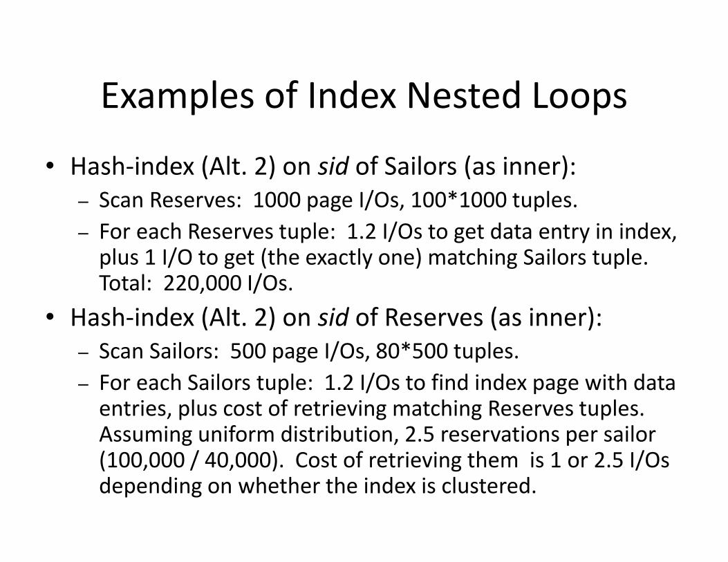
Examples of Index Nested Loops
• Hash-index (Alt. 2) on sid of Sailors (as inner):
– Scan Reserves: 1000 page I/Os, 100*1000 tuples.
– For each Reserves tuple: 1.2 I/Os to get data entry in index, plus 1 I/O to get (the exactly one) matching Sailors tuple. Total: 220,000 I/Os.
• Hash-index (Alt. 2) on sid of Reserves (as inner):
– Scan Sailors: 500 page I/Os, 80*500 tuples.
– For each Sailors tuple: 1.2 I/Os to find index page with data entries, plus cost of retrieving matching Reserves tuples. Assuming uniform distribution, 2.5 reservations per sailor (100,000 / 40,000). Cost of retrieving them is 1 or 2.5 I/Os depending on whether the index is clustered.
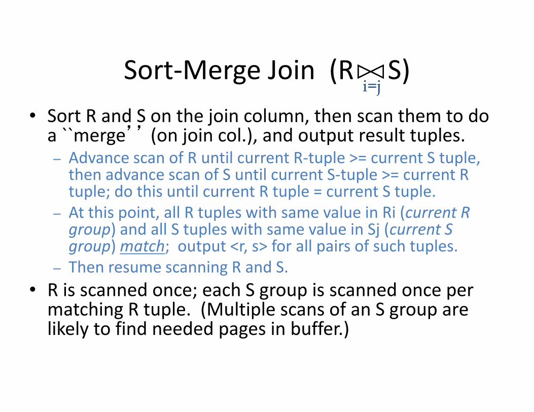
Sort-Merge Join (R S)
• Sort R and S on the join column, then scan them to do a ``merge’’ (on join col.), and output result tuples.– Advance scan of R until current R-tuple >= current S tuple,
then advance scan of S until current S-tuple >= current R tuple; do this until current R tuple = current S tuple.
– At this point, all R tuples with same value in Ri (current R group) and all S tuples with same value in Sj (current S group) match; output <r, s> for all pairs of such tuples.
– Then resume scanning R and S.
• R is scanned once; each S group is scanned once per matching R tuple. (Multiple scans of an S group are likely to find needed pages in buffer.)
><i=j
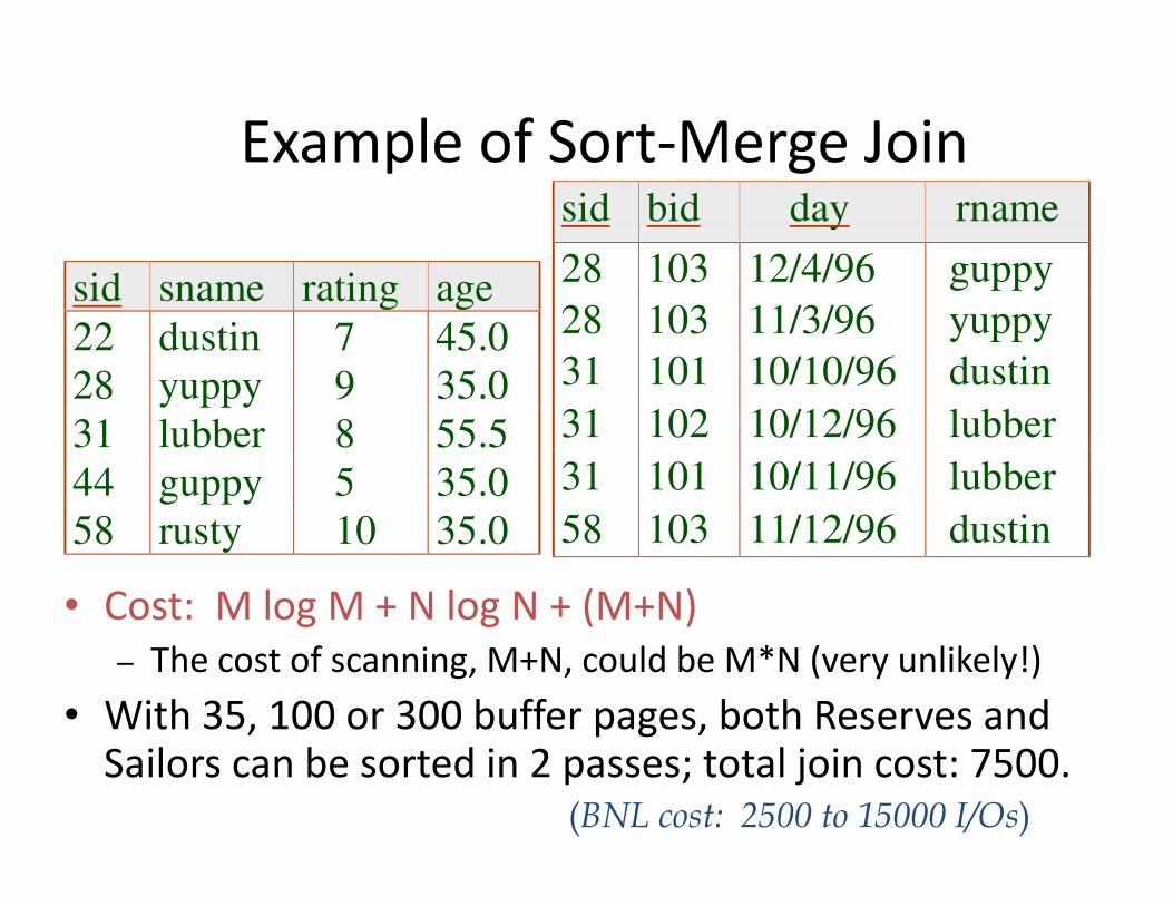
Example of Sort-Merge Join
• Cost: M log M + N log N + (M+N)
– The cost of scanning, M+N, could be M*N (very unlikely!)
• With 35, 100 or 300 buffer pages, both Reserves and Sailors can be sorted in 2 passes; total join cost: 7500.
sid sname rating age
22 dustin 7 45.0
28 yuppy 9 35.0
31 lubber 8 55.5
44 guppy 5 35.0
58 rusty 10 35.0
sid bid day rname
28 103 12/4/96 guppy
28 103 11/3/96 yuppy
31 101 10/10/96 dustin
31 102 10/12/96 lubber
31 101 10/11/96 lubber
58 103 11/12/96 dustin
(BNL cost: 2500 to 15000 I/Os)
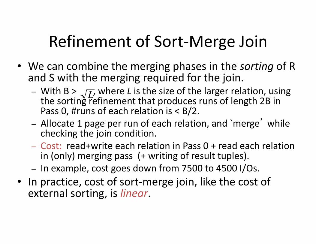
Refinement of Sort-Merge Join
• We can combine the merging phases in the sorting of R and S with the merging required for the join.– With B > , where L is the size of the larger relation, using
the sorting refinement that produces runs of length 2B in Pass 0, #runs of each relation is < B/2.
– Allocate 1 page per run of each relation, and `merge’ while checking the join condition.
– Cost: read+write each relation in Pass 0 + read each relation in (only) merging pass (+ writing of result tuples).
– In example, cost goes down from 7500 to 4500 I/Os.
• In practice, cost of sort-merge join, like the cost of external sorting, is linear.
L
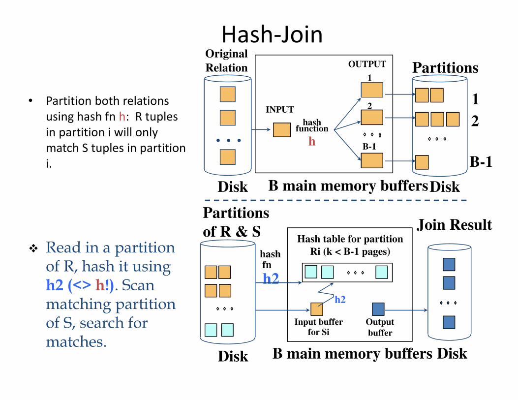
Hash-Join
• Partition both relations
using hash fn h: R tuples
in partition i will only
match S tuples in partition
i.
� Read in a partition of R, hash it using h2 (<> h!). Scan matching partition of S, search for matches.
Partitions
of R & S
Input bufferfor Si
Hash table for partition
Ri (k < B-1 pages)
B main memory buffersDisk
Output
buffer
Disk
Join Result
hashfn
h2
h2
B main memory buffersDiskDisk
Original
Relation OUTPUT
2INPUT
1
hashfunction
h B-1
Partitions
1
2
B-1
. . .
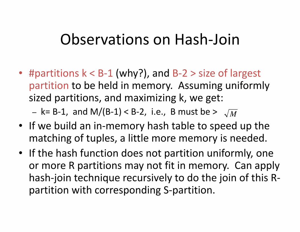
Observations on Hash-Join
• #partitions k < B-1 (why?), and B-2 > size of largest partition to be held in memory. Assuming uniformly sized partitions, and maximizing k, we get:
– k= B-1, and M/(B-1) < B-2, i.e., B must be >
• If we build an in-memory hash table to speed up the matching of tuples, a little more memory is needed.
• If the hash function does not partition uniformly, one or more R partitions may not fit in memory. Can apply hash-join technique recursively to do the join of this R-partition with corresponding S-partition.
M
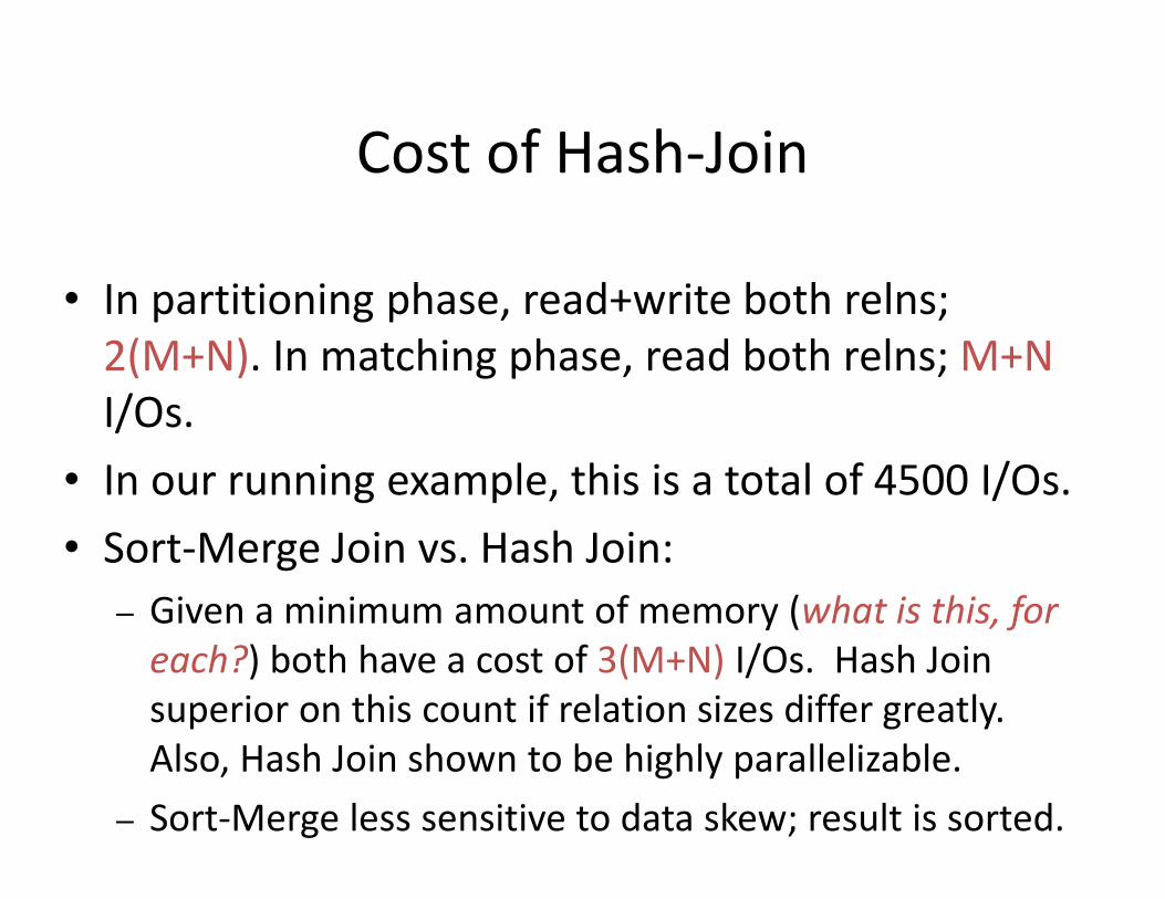
Cost of Hash-Join
• In partitioning phase, read+write both relns;
2(M+N). In matching phase, read both relns; M+N
I/Os.
• In our running example, this is a total of 4500 I/Os.
• Sort-Merge Join vs. Hash Join:
– Given a minimum amount of memory (what is this, for
each?) both have a cost of 3(M+N) I/Os. Hash Join
superior on this count if relation sizes differ greatly.
Also, Hash Join shown to be highly parallelizable.
– Sort-Merge less sensitive to data skew; result is sorted.
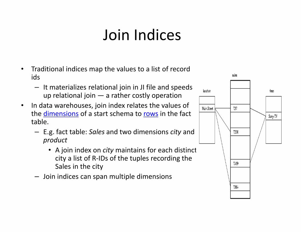
Join Indices
• Traditional indices map the values to a list of record ids
– It materializes relational join in JI file and speeds up relational join — a rather costly operation
• In data warehouses, join index relates the values of the dimensions of a start schema to rows in the fact table.
– E.g. fact table: Sales and two dimensions city and product
• A join index on city maintains for each distinct city a list of R-IDs of the tuples recording the Sales in the city
– Join indices can span multiple dimensions
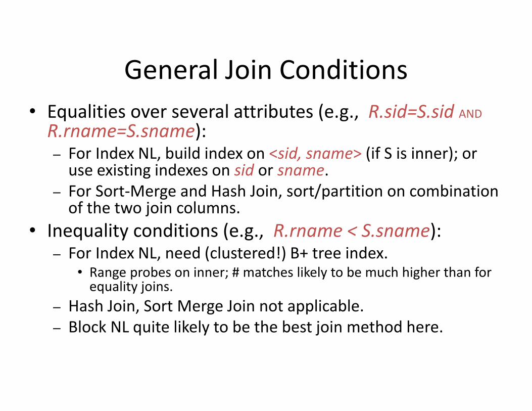
General Join Conditions
• Equalities over several attributes (e.g., R.sid=S.sid AND
R.rname=S.sname):– For Index NL, build index on <sid, sname> (if S is inner); or
use existing indexes on sid or sname.
– For Sort-Merge and Hash Join, sort/partition on combination of the two join columns.
• Inequality conditions (e.g., R.rname < S.sname):– For Index NL, need (clustered!) B+ tree index.
• Range probes on inner; # matches likely to be much higher than for equality joins.
– Hash Join, Sort Merge Join not applicable.
– Block NL quite likely to be the best join method here.
An invention in 2000s:
Column Stores for OLAP
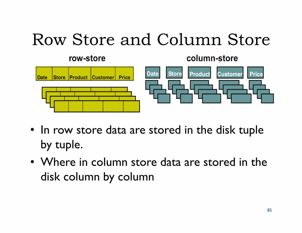
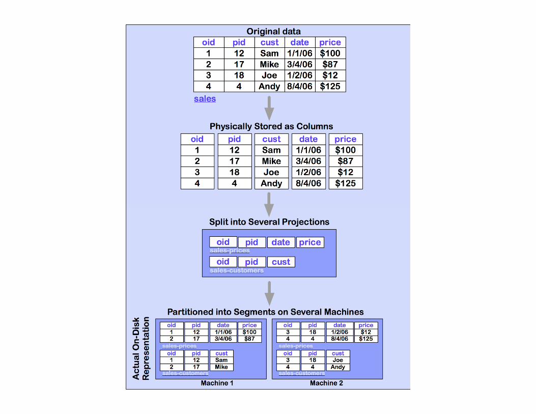
Row Store and Column Store
• In row store data are stored in the disk tuple by tuple.
• Where in column store data are stored in the disk column by column
85
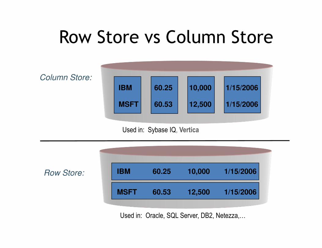
Row Store vs Column Store
IBM 60.25 10,000 1/15/2006
MSFT 60.53 12,500 1/15/2006
Row Store:
Used in: Oracle, SQL Server, DB2, Netezza,…
IBM 60.25 10,000 1/15/2006
MSFT 60.53 12,500 1/15/2006
Column Store:
Used in: Sybase IQ, Vertica
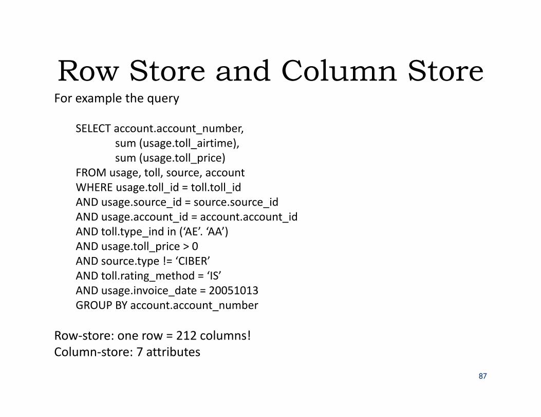
Row Store and Column StoreFor example the query
SELECT account.account_number,
sum (usage.toll_airtime),
sum (usage.toll_price)
FROM usage, toll, source, account
WHERE usage.toll_id = toll.toll_id
AND usage.source_id = source.source_id
AND usage.account_id = account.account_id
AND toll.type_ind in (‘AE’. ‘AA’)
AND usage.toll_price > 0
AND source.type != ‘CIBER’
AND toll.rating_method = ‘IS’
AND usage.invoice_date = 20051013
GROUP BY account.account_number
Row-store: one row = 212 columns!
Column-store: 7 attributes
87
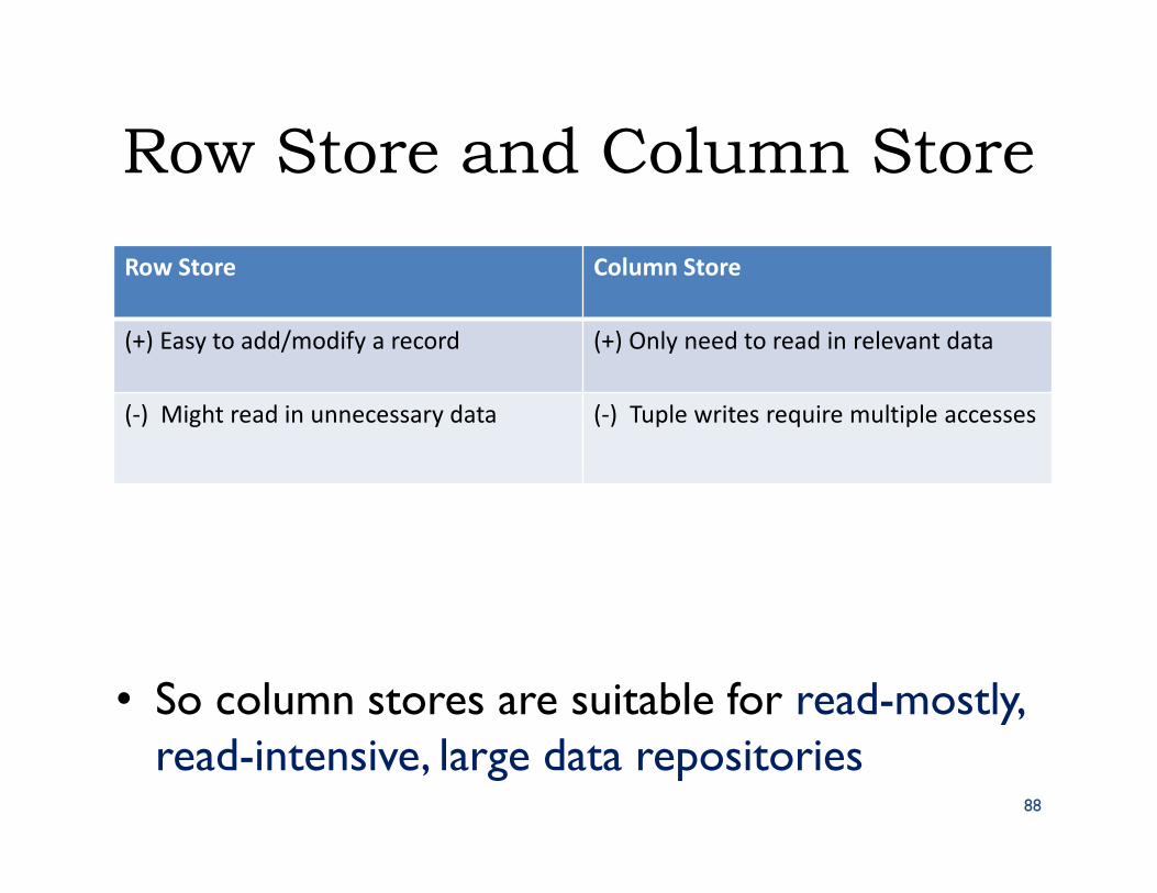
Row Store and Column Store
• So column stores are suitable for read-mostly, read-intensive, large data repositories
Row Store Column Store
(+) Easy to add/modify a record (+) Only need to read in relevant data
(-) Might read in unnecessary data (-) Tuple writes require multiple accesses
88
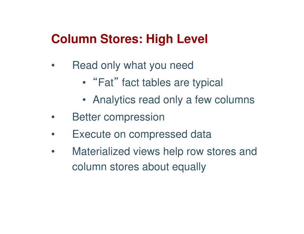
Column Stores: High Level
• Read only what you need
• “Fat” fact tables are typical
• Analytics read only a few columns
• Better compression
• Execute on compressed data
• Materialized views help row stores and
column stores about equally
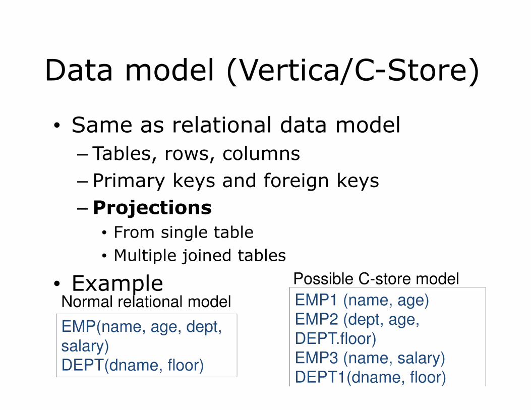
Data model (Vertica/C-Store)
• Same as relational data model
– Tables, rows, columns
– Primary keys and foreign keys
– Projections
• From single table
• Multiple joined tables
• ExampleEMP1 (name, age)
EMP2 (dept, age,
DEPT.floor)
EMP3 (name, salary)
DEPT1(dname, floor)
EMP(name, age, dept,
salary)
DEPT(dname, floor)
Normal relational model
Possible C-store model
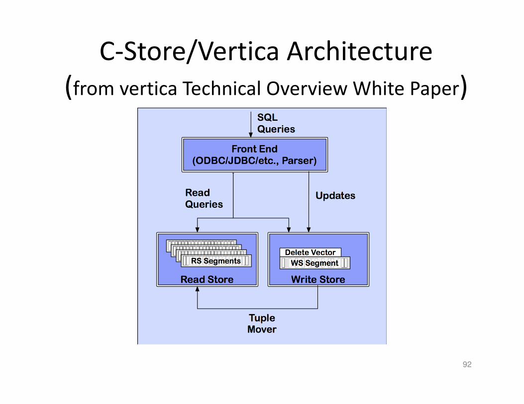
C-Store/Vertica Architecture
(from vertica Technical Overview White Paper)
92
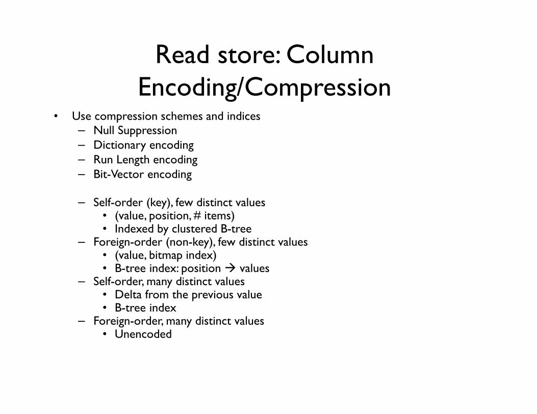
Read store: Column Encoding/Compression
• Use compression schemes and indices– Null Suppression– Dictionary encoding– Run Length encoding– Bit-Vector encoding
– Self-order (key), few distinct values• (value, position, # items)• Indexed by clustered B-tree
– Foreign-order (non-key), few distinct values• (value, bitmap index)• B-tree index: position � values
– Self-order, many distinct values• Delta from the previous value• B-tree index
– Foreign-order, many distinct values• Unencoded
Compression
• Trades I/O for CPU
– Increased column-store opportunities:
– Higher data value locality in column stores
– Techniques such as run length encoding far more useful
94
Write Store
• Same structure, but explicitly use (segment, key) to identify records– Easier to maintain the mapping – Only concerns the inserted records
• Tuple mover– Copies batch of records to RS
• Delete record– Mark it on RS– Purged by tuple mover
How to solve read/write conflict
• Situation: one transaction updates the record X, while another transaction reads X.
• Use snapshot isolation
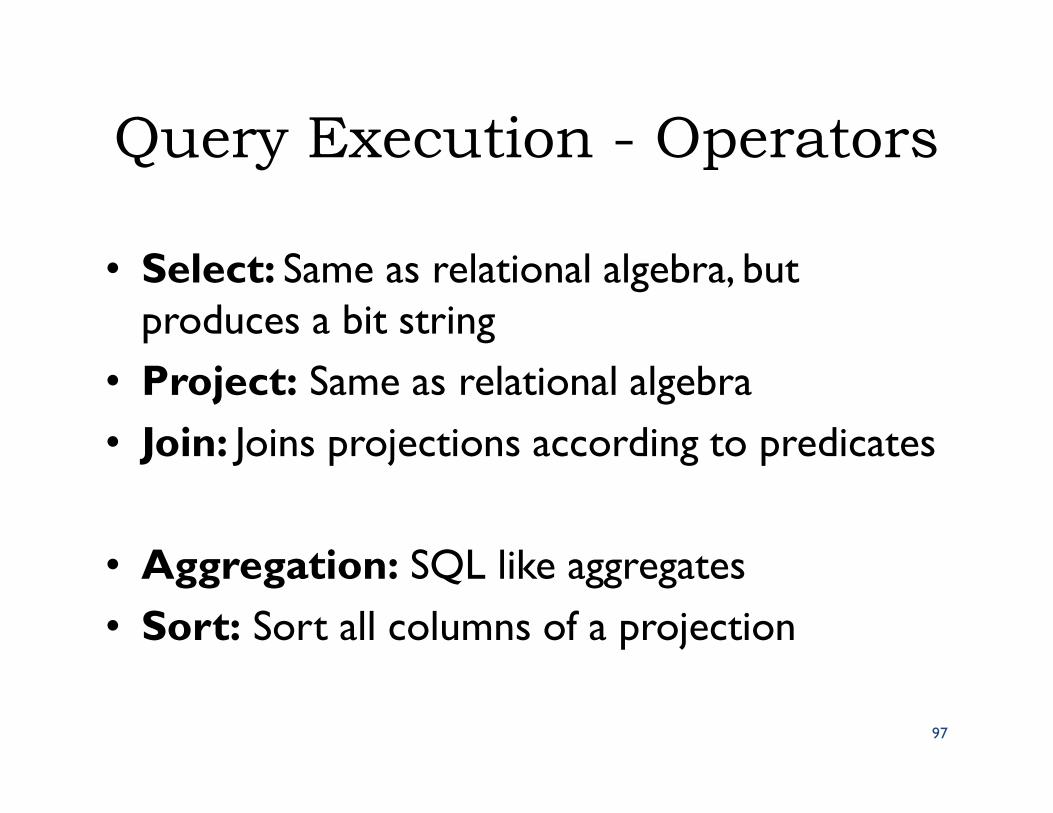
Query Execution - Operators
• Select: Same as relational algebra, but produces a bit string
• Project: Same as relational algebra
• Join: Joins projections according to predicates
• Aggregation: SQL like aggregates
• Sort: Sort all columns of a projection
97
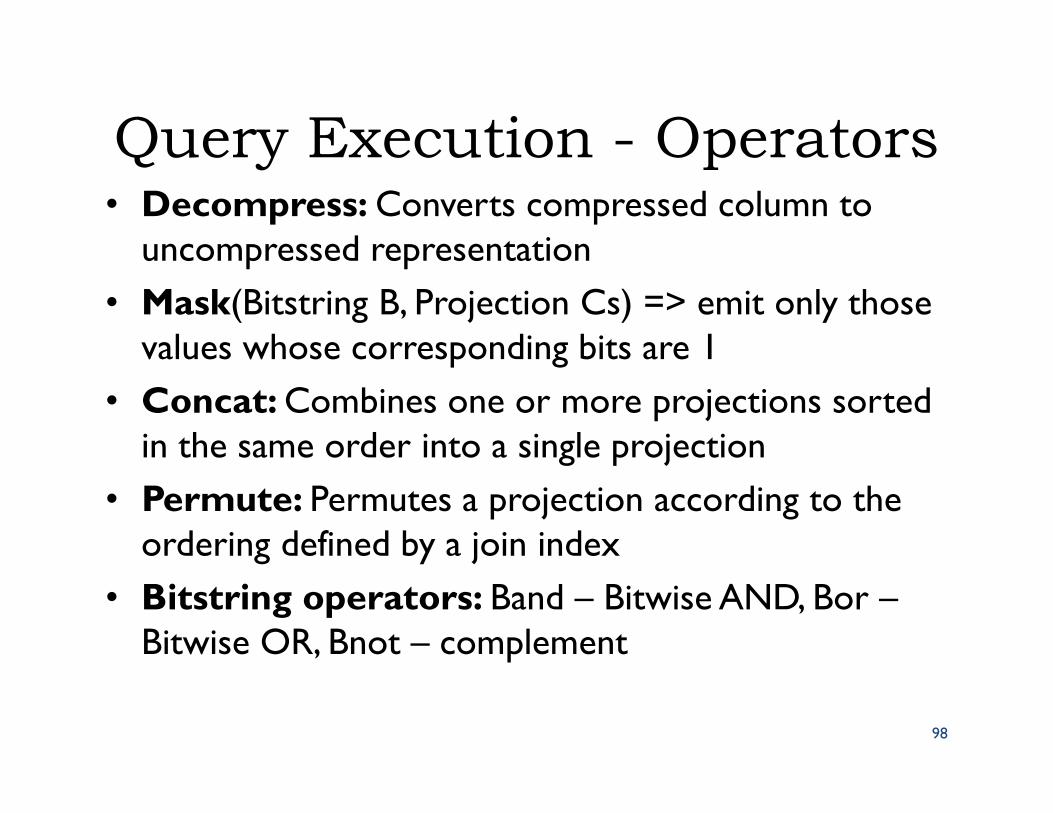
Query Execution - Operators• Decompress: Converts compressed column to
uncompressed representation
• Mask(Bitstring B, Projection Cs) => emit only those values whose corresponding bits are 1
• Concat: Combines one or more projections sorted in the same order into a single projection
• Permute: Permutes a projection according to the ordering defined by a join index
• Bitstring operators: Band – Bitwise AND, Bor –Bitwise OR, Bnot – complement
98
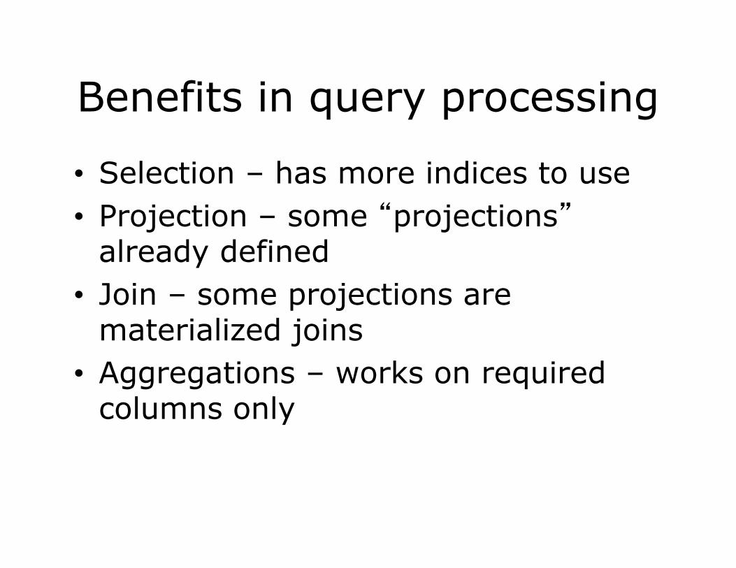
Benefits in query processing
• Selection – has more indices to use
• Projection – some “projections”already defined
• Join – some projections are materialized joins
• Aggregations – works on required columns only
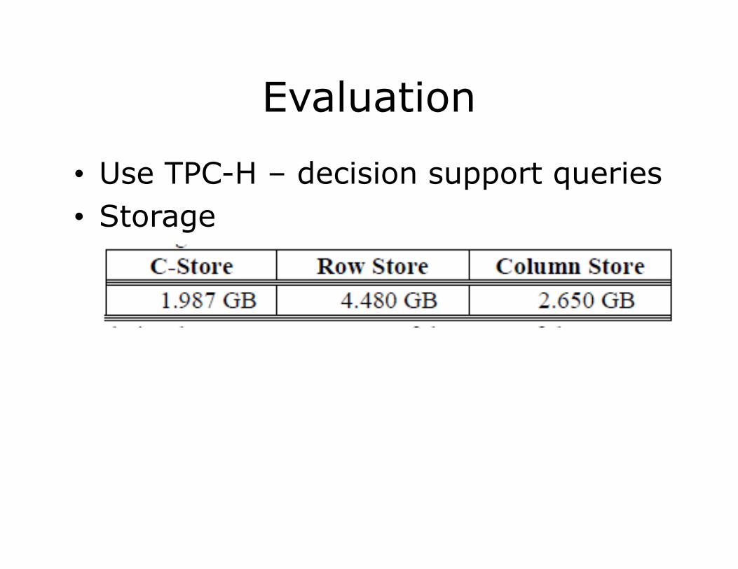
Evaluation
• Use TPC-H – decision support queries
• Storage
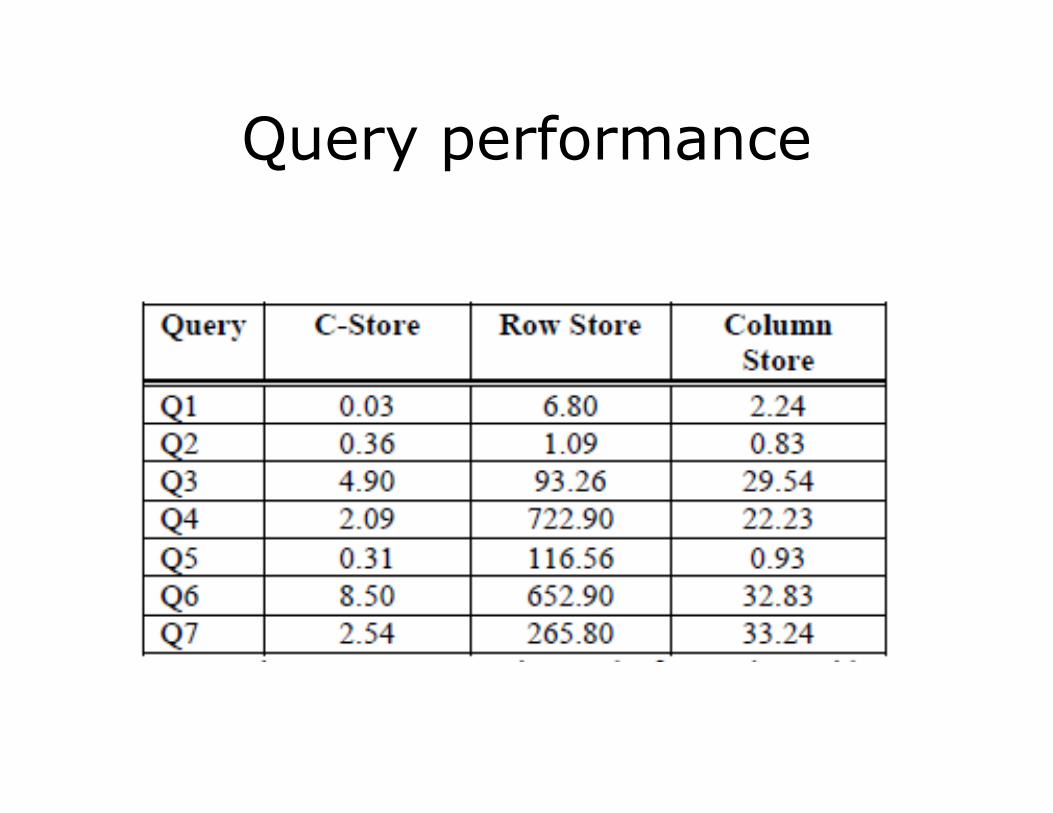
Query performance
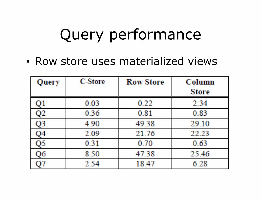
Query performance
• Row store uses materialized views
Summary: the performance gain
• Column representation – avoids reads of unused attributes
• Storing overlapping projections – multiple orderings of a column, more choices for query optimization
• Compression of data – more orderings of a column in the same amount of space
• Query operators operate on compressed representation
Google’s Dremel:
Interactive Analysis of Web-Scale Datasets
104
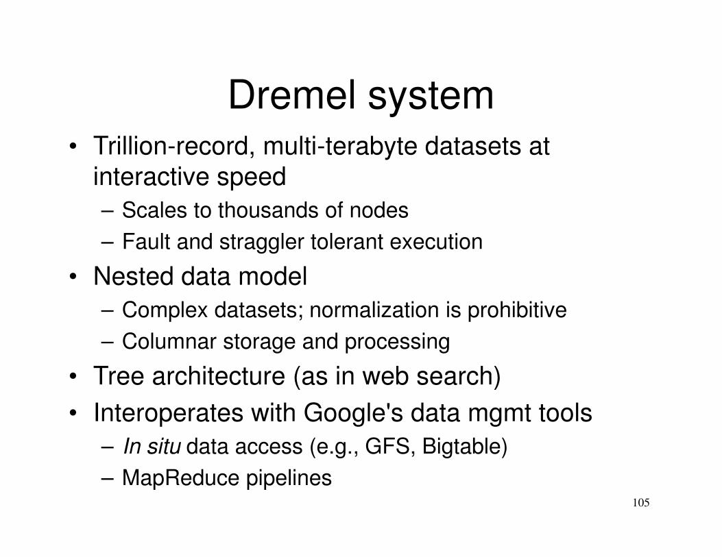
Dremel system• Trillion-record, multi-terabyte datasets at
interactive speed
– Scales to thousands of nodes
– Fault and straggler tolerant execution
• Nested data model
– Complex datasets; normalization is prohibitive
– Columnar storage and processing
• Tree architecture (as in web search)
• Interoperates with Google's data mgmt tools
– In situ data access (e.g., GFS, Bigtable)
– MapReduce pipelines105
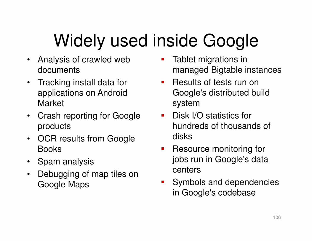
Widely used inside Google
106
• Analysis of crawled web
documents
• Tracking install data for
applications on Android
Market
• Crash reporting for Google
products
• OCR results from Google
Books
• Spam analysis
• Debugging of map tiles on
Google Maps
� Tablet migrations in
managed Bigtable instances
� Results of tests run on
Google's distributed build
system
� Disk I/O statistics for
hundreds of thousands of
disks
� Resource monitoring for
jobs run in Google's data
centers
� Symbols and dependencies
in Google's codebase
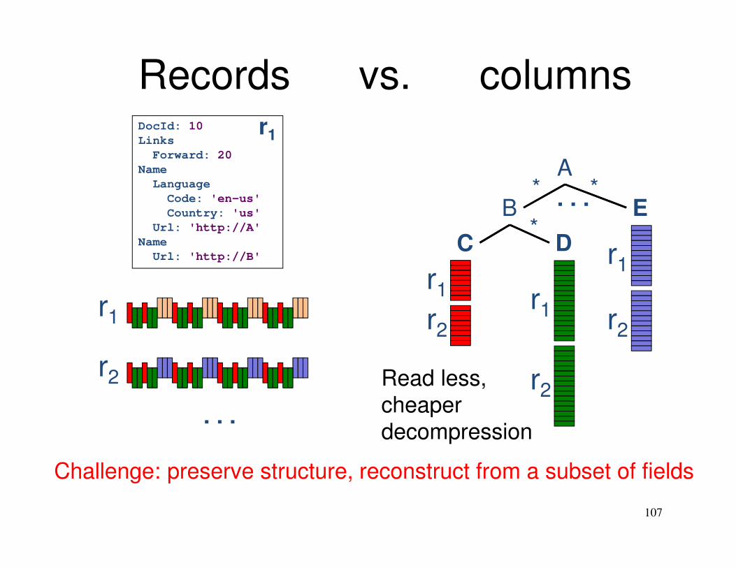
Records vs. columns
107
A
B
C D
E*
*
*
. . .
. . .
r1
r2
r1
r2
r1
r2
r1
r2
Challenge: preserve structure, reconstruct from a subset of fields
Read less,
cheaper
decompression
DocId: 10
Links
Forward: 20
Name
Language
Code: 'en-us'
Country: 'us'
Url: 'http://A'
Name
Url: 'http://B'
r1
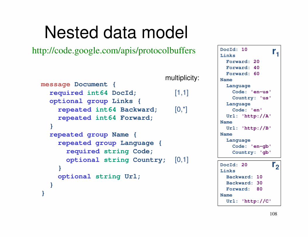
Nested data model
108
message Document {
required int64 DocId; [1,1]optional group Links {
repeated int64 Backward; [0,*]repeated int64 Forward;
}
repeated group Name {
repeated group Language {
required string Code;
optional string Country; [0,1]}
optional string Url;
}
}
DocId: 10
Links
Forward: 20
Forward: 40
Forward: 60
Name
Language
Code: 'en-us'
Country: 'us'
Language
Code: 'en'
Url: 'http://A'
Name
Url: 'http://B'
Name
Language
Code: 'en-gb'
Country: 'gb'
r1
DocId: 20
Links
Backward: 10
Backward: 30
Forward: 80
Name
Url: 'http://C'
r2
http://code.google.com/apis/protocolbuffers
multiplicity:
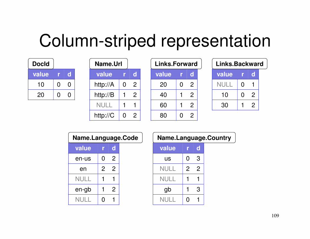
Column-striped representation
value r d
10 0 0
20 0 0
109
value r d
20 0 2
40 1 2
60 1 2
80 0 2
value r d
NULL 0 1
10 0 2
30 1 2
DocId
value r d
http://A 0 2
http://B 1 2
NULL 1 1
http://C 0 2
Name.Url
value r d
en-us 0 2
en 2 2
NULL 1 1
en-gb 1 2
NULL 0 1
Name.Language.Code Name.Language.Country
Links.BackwardLinks.Forward
value r d
us 0 3
NULL 2 2
NULL 1 1
gb 1 3
NULL 0 1
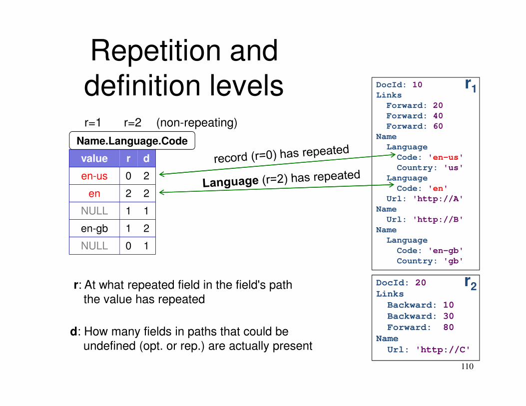
Repetition and
definition levels
110
DocId: 10
Links
Forward: 20
Forward: 40
Forward: 60
Name
Language
Code: 'en-us'
Country: 'us'
Language
Code: 'en'
Url: 'http://A'
Name
Url: 'http://B'
Name
Language
Code: 'en-gb'
Country: 'gb'
r1
DocId: 20
Links
Backward: 10
Backward: 30
Forward: 80
Name
Url: 'http://C'
r2
value r d
en-us 0 2
en 2 2
NULL 1 1
en-gb 1 2
NULL 0 1
Name.Language.Code
r: At what repeated field in the field's path
the value has repeated
d: How many fields in paths that could be
undefined (opt. or rep.) are actually present
r=2r=1 (non-repeating)
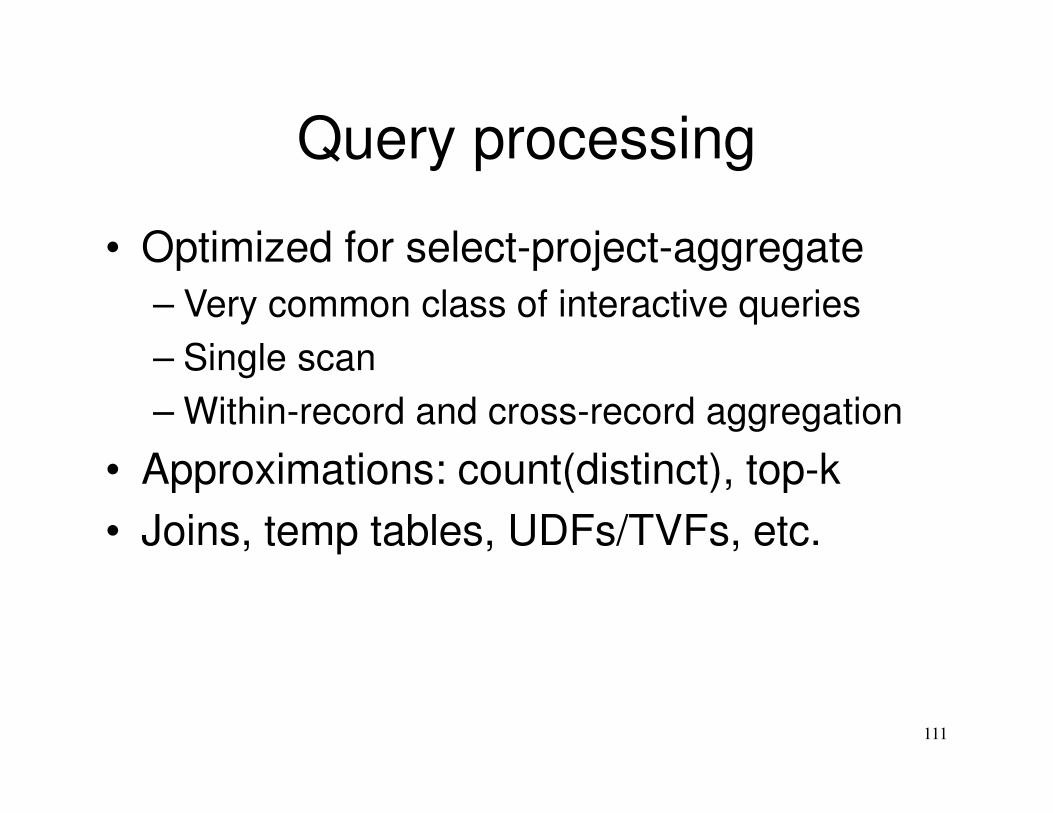
Query processing
• Optimized for select-project-aggregate
– Very common class of interactive queries
– Single scan
– Within-record and cross-record aggregation
• Approximations: count(distinct), top-k
• Joins, temp tables, UDFs/TVFs, etc.
111
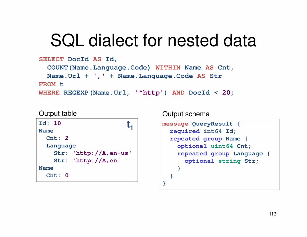
SQL dialect for nested data
112
Id: 10
Name
Cnt: 2
Language
Str: 'http://A,en-us'
Str: 'http://A,en'
Name
Cnt: 0
t1
SELECT DocId AS Id,
COUNT(Name.Language.Code) WITHIN Name AS Cnt,
Name.Url + ',' + Name.Language.Code AS Str
FROM t
WHERE REGEXP(Name.Url, '^http') AND DocId < 20;
message QueryResult {
required int64 Id;
repeated group Name {
optional uint64 Cnt;
repeated group Language {
optional string Str;
}
}
}
Output table Output schema
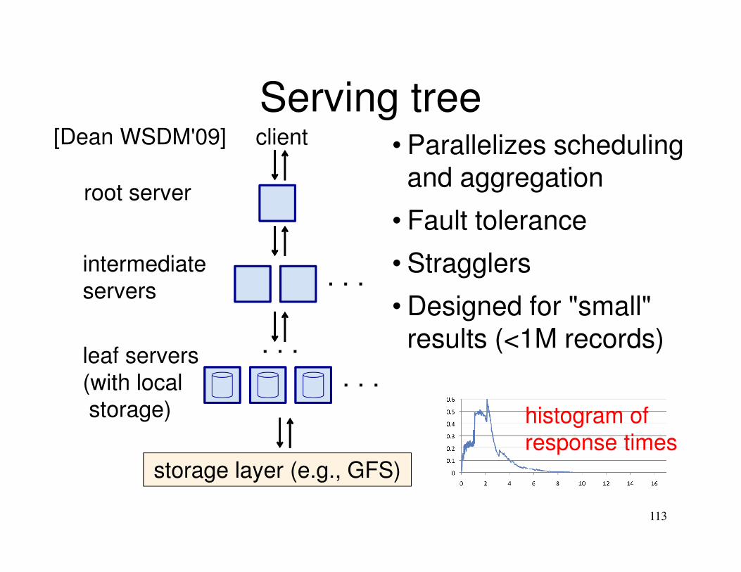
Serving tree
113
storage layer (e.g., GFS)
. . .
. . .
. . .leaf servers
(with local
storage)
intermediate
servers
root server
client • Parallelizes scheduling and aggregation
• Fault tolerance
• Stragglers
• Designed for "small" results (<1M records)
[Dean WSDM'09]
histogram of
response times
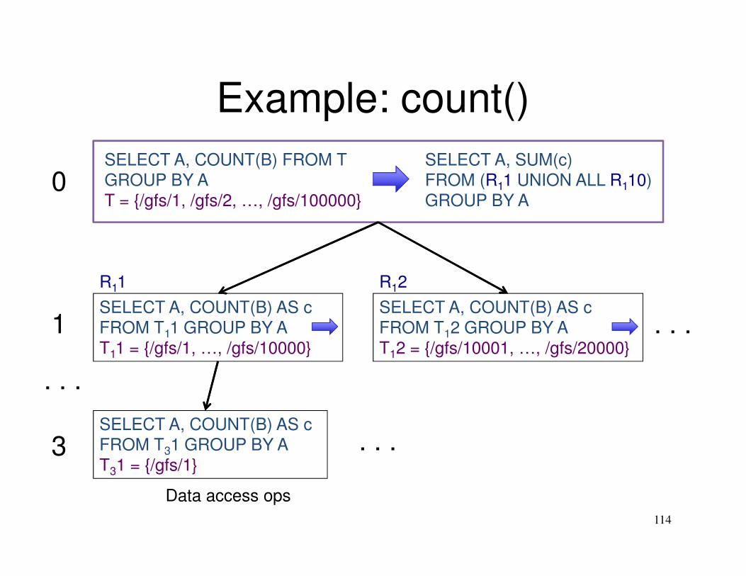
Example: count()
114
SELECT A, COUNT(B) FROM T
GROUP BY A
T = {/gfs/1, /gfs/2, …, /gfs/100000}
SELECT A, SUM(c)
FROM (R11 UNION ALL R110)
GROUP BY A
SELECT A, COUNT(B) AS c
FROM T11 GROUP BY A
T11 = {/gfs/1, …, /gfs/10000}
SELECT A, COUNT(B) AS c
FROM T12 GROUP BY A
T12 = {/gfs/10001, …, /gfs/20000}
SELECT A, COUNT(B) AS c
FROM T31 GROUP BY A
T31 = {/gfs/1}
. . .
0
1
3
R11 R12
Data access ops
. . .
. . .
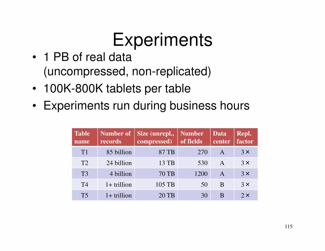
Experiments
Table
name
Number of
records
Size (unrepl.,
compressed)
Number
of fields
Data
center
Repl.
factor
T1 85 billion 87 TB 270 A 3×
T2 24 billion 13 TB 530 A 3×
T3 4 billion 70 TB 1200 A 3×
T4 1+ trillion 105 TB 50 B 3×
T5 1+ trillion 20 TB 30 B 2×
115
• 1 PB of real data(uncompressed, non-replicated)
• 100K-800K tablets per table
• Experiments run during business hours
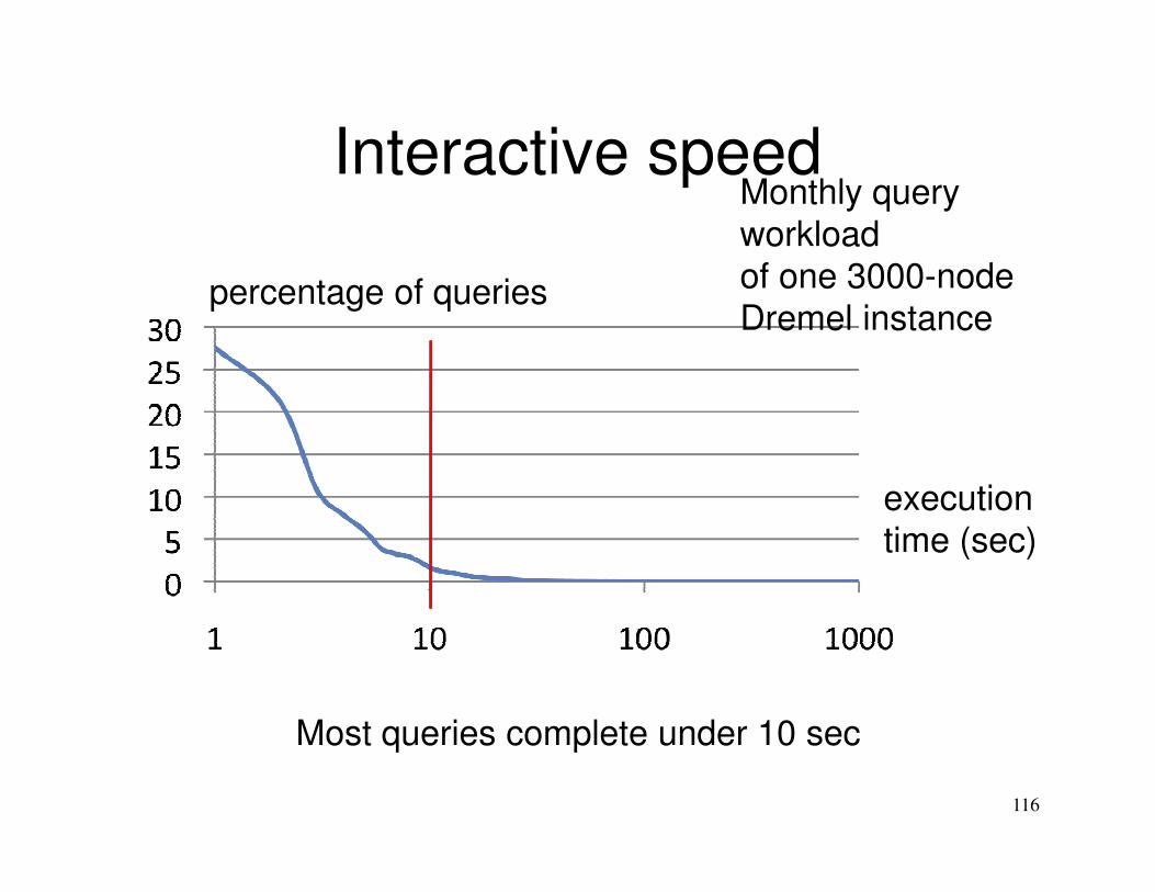
Interactive speed
116
execution
time (sec)
percentage of queries
Most queries complete under 10 sec
Monthly query
workload
of one 3000-node
Dremel instance
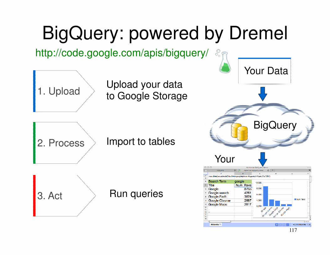
BigQuery: powered by Dremel
117
http://code.google.com/apis/bigquery/
1. Upload
2. Process
Upload your datato Google Storage
Import to tables
Run queries3. Act
Your Data
BigQuery
Your Apps
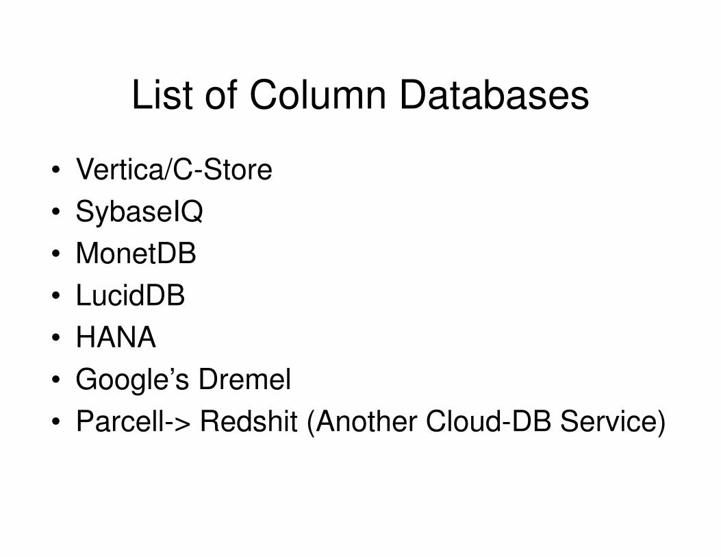
List of Column Databases
• Vertica/C-Store
• SybaseIQ
• MonetDB
• LucidDB
• HANA
• Google’s Dremel
• Parcell-> Redshit (Another Cloud-DB Service)
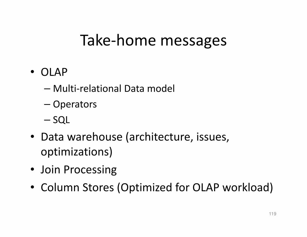
Take-home messages
• OLAP
– Multi-relational Data model
– Operators
– SQL
• Data warehouse (architecture, issues,
optimizations)
• Join Processing
• Column Stores (Optimized for OLAP workload)
119


![[Materi] Data Warehouse, Data Mart, OLAP, Dan Data Mining](https://img.pdfslide.net/doc/110x75/577c7cf61a28abe0549cc769/materi-data-warehouse-data-mart-olap-dan-data-mining.jpg)