Copyright © 2012 by Humberto Brea-Solís, Ramon Casadesus-Masanell, and Emili Grifell-Tatjé

Working papers are in draft form. This working paper is distributed for purposes of comment and discussion only. It may not be reproduced without permission of the copyright holder. Copies of working papers are available from the author.

Business Model Evaluation: Quantifying Walmart’s Sources of Advantage Humberto Brea-Solís Ramon Casadesus-Masanell Emili Grifell-Tatjé

Working Paper

13-039 November 6, 2012

Business Model Evaluation:

Quantifying Walmart’s Sources of Advantage*

November 6, 2012

Humberto Brea-Solís† Ramon Casadesus-Masanell‡ Emili Grifell-Tatjé§

A B S T R A C T

In recent years, the concept of the business model has received substantial attention in the strategy literature, where a number of qualitative approaches to describe, represent, and evaluate business models have been proposed. We contend that while helpful to understand a firm’s overall logic of value creation and capture, qualitative methods must be complemented with quantitative analyses. The development of quantitative methods for the study of business models, however, has trailed that of their qualitative peers. In this paper, we develop an analytical framework based on the theory of index numbers and production theory to provide quantitative insight on the link between a firm’s business model choices and their ultimate profit consequences. We apply the method to Walmart. Using evidence from annual reports, research papers, case studies, and books for the period of 1972-2008, we build a qualitative representation of Walmart’s business model. We then map that representation to an analytical model that quantifies Walmart’s sources of competitive advantage over a 36-year period. Although Walmart’s business model remained the same during the years of our study, we find that the different CEOs pulled a number of business model levers differently, which partly explains the variation in Walmart’s performance throughout the years. Under Sam Walton, the company’s performance improved due mainly to the adoption of new technologies as well as low prices obtained from vendors. David Glass’s tenure was characterized by business model choices aimed at increasing volume such as building new stores, increasing product variety, everyday low prices (EDLP), and high-powered incentives for store managers. Input and output prices played a smaller role under David Glass than under Sam Walton. Finally, Lee Scott loosened EDLP and modified Walmart’s human resource practices by offering better benefits and wages to associates in response to growing social pressure. Overall, our analysis suggests that the effectiveness of a particular business model depends not only on its design (its levers and how they relate to one another) but, most importantly, on its implementation (how the business model levers are pulled).

* For helpful comments, we thank C.A.K Lovell from the University of Queensland (Australia) and seminar participants at the XI European Workshop of Efficiency and Productivity Analysis in Pisa and the III DEMO June Workshop, Economics of Organizations, Corporate Governance and Competitiveness, Barcelona. Brea-Solís thanks l’Agència de Gestió d’Ajuts Universitaris i de Recerca de la Generalitat de Catalunya for financial support. Casadesus-Masanell thanks the HBS Division of Research. Grifell-Tatjé thanks the Spanish Ministry of Science and Technology (ECO2010-21242-C03-01) and the Generalitat de Catalunya (2009SGR 1001) for financial support. † HEC Management School, ULg. ‡ Harvard Business School. § Business Department, Universitat Autònoma de Barcelona.

1

1. Introduction

In recent years the strategy field has become increasingly interested in the study of

business models.1 Although the expression was introduced long ago by Peter Drucker,2

academic work on business models began just a decade ago in the context of the Internet

boom, where entrepreneurs were asked to explain how their ventures would create value (the

wedge between customer willingness to pay and supplier willingness to sell, see

Brandenburger and Stuart, 1996) and how value would be captured as profit. Indeed, the most

common definition of business model is “the logic of the firm, the way it operates, and how it

creates and captures value for its stakeholders.”3

Casadesus-Masanell and Ricart (2008, 2010, 2011) and Casadesus-Masanell and Zhu

(2010) operationalize this notion by decomposing business models into two fundamental

elements: choices—such as policies, assets, and governance of policies and assets—and the

consequences of these choices. The causal links between choices and consequences help

explain the logic of the firm, how it creates and captures value for its stakeholders. These

authors also propose a methodology to represent business models qualitatively.

While business model representations help improve an analyst’s understanding of a

firm’s value logic, the methodology proposed offers little guidance on how the causal links

between choices and consequences can be quantified. Without quantification, a detailed study

of a firm’s business model is incomplete because there is often too much freedom on how to

interpret relationships between firm choices (such as low prices, heavy investment in

technology, or high-powered incentives for managers) and their consequences (such as

volume, bargaining power with suppliers, or a culture of frugality).

In this paper we propose a novel approach to quantify the link between a firm’s choices

and their consequences and, ultimately, for gaining a better understanding of the virtues and

weaknesses of a firm’s business model. The method builds on recent advances in production

theory and index numbers by Grifell-Tatjé and Lovell (1999, 2008, 2012) and relates business

model choices to profit variations over time. Its starting point is the observation that profits

raise and fall for two reasons: changes in either prices or quantities. In particular, a firm’s

profits could increase for any of the following reasons: (a) selling goods at higher prices; (b)

paying less for inputs, such as labor or capital; (c) selling more goods while holding constant

2

their cost markup; or (d) using fewer inputs per unit of good produced/sold. Note that (a) and

(b) are related to prices whereas (c) and (d) are related to quantities. Our method quantifies

how much of a firm’s profit variation is due to price and how much is due to quantity effects.

These two effects, in turn, are determined through business model choices.

[INSERT FIGURE 1 ABOUT HERE]

Indeed, the key to our approach is the realization that, at heart, business models create

and capture value by acting on prices and volumes. For instance, Ryanair—a company that

competes through a generic low-cost strategy—has made business model choices, such as

flying to secondary airports or the use of a standardized fleet of 737s, that have led to lower

input prices. Likewise, Ryanair has chosen to maximize the number of seats in its aircraft by

offering coach service only and removing the kitchenette, which has led to larger volumes.

Thus, a quantification Ryanair’s profit variation over time due to prices and to volumes shall

provide valuable information on how the firm’s business model works.

As noted, the analytical framework that we propose combines the theory of index

numbers and production theory, uses publicly available information about realized prices and

volumes, and has two levels of analysis.4 The first level uses index numbers to produce an

aggregated estimate of the price and quantity effects.5 In particular, we build Bennet-type

indicators for prices and quantities of inputs (e.g., labor and capital) and outputs (e.g., final

products).6 The price effect obtained through index numbers is useful to quantify, for example,

the impact of business model policies that affect prices of inputs and outputs (e.g., product

range or new supply sources) on profits. The quantity effect, in turn, captures the impact of

policies that affect quantity (e.g., hiring more staff or investment in larger stores) on the

bottom line.

The second level of analysis builds on new developments in production theory to

decompose the quantity effect into an operational efficiency effect, a technological change

effect, and an activity effect. To do this, we build on well-established techniques in production

theory. This requires the assembly of a dataset that records information about other firms in

the industry. We use production frontiers as reference points for computing the operational

efficiency, technological change, and activity effects.

3

The operational efficiency effect measures how much profit variation over time is due to

better use of input quantities; that is, how close the firm is to the production possibility

frontier. The technological progress effect captures profit variation caused by the introduction

of technological improvements that allow firms to produce with fewer inputs. Conceptually,

technological progress corresponds to an expansion of the production possibility frontier. The

activity effect measures how much the variation of profits over time is due to sales volume and

the volume of inputs employed. This corresponds to a movement along the production

possibility frontier. Our method quantifies these three effects. The additional level of detail

obtained helps us better understand how a firm’s choices leading to growth contribute to

higher profits. It also helps us explore the effects of technological progress and the firm’s

efforts to achieve higher efficiency levels.

One important advantage of our approach is that it uses widely available accounting

data—of the focal firm and main competitors—and can therefore be applied broadly. If fine-

grained proprietary data are available, the framework can be refined further to deliver more

nuanced, less aggregated quantifications. To demonstrate how the method can be applied to

aggregate data to produce insights on how a firm’s business model operates, we apply the

methodology to study the evolution of Walmart’s business model since its IPO in 1971

through 2008.

Walmart constitutes an ideal setting to apply our approach and demonstrate its value

because: (i) there is a wealth of qualitative information about the company, which allows us to

build a detailed business model representation, and (ii) being a public company, the

accounting data that we need for the analysis are readily available. The company began

operations in 1962, when Sam Walton and his brother Bud failed to persuade Ben Franklin—

Sam Walton’s franchisor at the time—to open discount retail stores in rural America. The

unlikely success of this business venture had profound consequences worldwide. Fishman

(2006) points out that Walmart’s influence is felt everywhere, even in countries where there

are no Walmart stores. Indeed, Walmart alters other retailers’ business practices, provokes

changes in product features, affects urban space, sets industry standards, changes market

structure, and influences the consumer habits of millions of people worldwide. Walmart’s

sales in 2010, worth $420 billion, placed the company as the 25th largest economy in the world

if its sales were likened to a country’s GDP.

4

Using evidence from annual reports, research papers, case studies, and books on

Walmart, we describe the company’s business model choices over time. We then build a

quantitative model that can be used to determine the effect of Walmart’s choices on its

competitive advantage. For the quantitative analysis, we construct a dataset that includes the

largest firms in the American discount retailing industry to define—using methods developed

in the literature on production theory—a best practice production frontier. Specifically, we use

labor and capital as inputs, and value added as the measure of output. We compute the effect

of operational efficiency, new technological improvements, level of activity, and prices on

Walmart’s profits during the period 1972-2008. During this period Walmart had three CEOs:

Sam Walton (until 1988), David Glass (from 1988 to 2000), and Lee Scott (from 2000).

We find that input and output prices, technological progress, and the level of activity

played different roles across the three CEOs. Under Sam Walton (1972-1988), Walmart

deepened its policy of everyday low prices (EDLP), which led to negative output price effects.

These were somewhat offset by favorable input price concessions obtained from vendors.

While price reductions to customers hurt profits, more favorable purchase prices from vendors

had a substantial positive effect. The analysis also reveals that under Sam Walton, Walmart

increased its profits substantially through the adoption of new technology (such as investment

on a satellite system, uniform product codes, or automated distribution centers) that pushed the

production possibility frontier outward. Finally, the activity effect—variations in the volume

of outputs and inputs that led to economies of scale, changes in the product mix and changes

in the input mix—explains the remainder profit variation during this period.

More than 100% of profit variation under David Glass (1988-2000) is explained by the

activity effect. Thus Walmart’s success during this period was due, primarily, to business

model choices aimed at increasing volume such as building new stores, increasing product

variety, setting low prices, and implementing high-powered incentives for store managers.

Technological improvements explain only a small fraction of the company’s profit variation

over this period. Output and input price effects played substantially smaller roles than during

Sam Walton’s tenure.

Our analysis reveals that Lee Scott (2000-2008) loosened EDLP and cost controls.

Indeed, value added per dollar sold and input prices—labor costs, mainly—were on the rise

5

under his tenure. Finally, our study indicates that by the early 1980s Walmart had become the

most efficient discount retailer in the United States (U.S.), a position it held through the end of

our sample. Thus, for most of the years of analysis Walmart was on the production possibility

frontier; only early during Sam Walton’s tenure profit variation was partly explained by gains

in operational effectiveness.

The rest of the paper is organized as follows. In Section 2 we review the literature on

business models. In Section 3, we describe and discuss Walmart’s most important business

model choices. In Section 4 we present our method for quantifying the relationships between

choices and consequences to connect the business model choices to data. In Section 5 we

describe the dataset for the analysis. Section 6 presents the results. Section 7 concludes with a

discussion of the advantages and drawbacks of our method.

2. The Concept of Business Model

The notion of business model is recent in the scholarly literature. In the 1990s, as new

ways of doing business that subverted established logics of value creation and value capture

emerged, practitioners employed the phrase to describe the ways in which untried e-business

ventures were to operate (Chesbrough and Rosenbloom, 2002; Magretta, 2002). The term was

thus used to describe a wide diversity of novel, heterodox e-commerce firms.

While helpful to refer to “the logic of the firm,” the notion is not free from controversy.

Porter (2001), for instance, has described the term as imprecise. This ambiguity has prompted

many attempts to establish its boundaries and define its components. Mäkinen and Seppänen

(2007) observe that most of these attempts were carried out in isolation from one another,

which partially explains the current state of fragmentation in definitions. Magretta (2002)

considers the terms “strategy” and “business model” not clearly separated and suggests that

concerted efforts to define them should be made. More recently, Lecocq, Demil, and Ventura

(2010) argued that the business model concept shows features of a research program based on

Lakatos’s viewpoint of scientific progress. In particular, the business model research program

has a “hard core” (fundamental assumptions concerning an object), a set of “protective

hypotheses” (hypotheses that are being debated and/or tested but do not yet constitute

generally accepted assumptions), and it is “dynamic.” Nevertheless, the authors claim that the

theorization stage is still in its infancy and, to make progress, it is necessary to operationalize

6

the concept. They conclude that new developments should aim at determining how business

models must be observed, qualified, and measured.

Despite these objections, the concept of a business model is useful for integrating

different, related elements. To Chesbrough and Rosenbloom (2002), for instance, a business

model is a device that establishes a link between technological development and economic

innovation. Hedman and Kalling (2003) regard the notion as an integrative concept that

connects the resource-based view and the industrial organization perspectives on strategy. And

Amit and Zott (2001) propose a unifying definition “that captures the value creation from

multiple sources.”

Although there are myriad definitions of “business model,” for the most part they are

similar. Magretta (2002), for example, defines it as a description of how the parts of a business

fit together. Hedman and Kalling (2003) characterize the concept as a description of the key

components of a business. The idea of business models composed of a predetermined

collection of elements seems to be hovering over most definitions. Several studies have

attempted to provide a definitive list of what a business model should include. Morris et al.

(2005) and Hedman and Kalling (2003) examine diverse suggestions for the components of a

business model. The range spans between three and eight elements. Morris et al (2005)

suggest a business model concept that answers six questions and has three different levels,

while Hedman and Kalling (2003) suggest seven components. The vocabulary employed to

describe these components differs considerably from definition to definition, reflecting the

lack of consensus among researchers.

In this study, we employ the conceptual framework developed by Casadesus-Masanell

and Ricart (2010). According to this view, a business model is composed of two types of

elements: choices made by the management and the consequences of these choices. There are

three types of choices: policies, assets, and governance of assets and policies. Policy choices

refer to courses of action that the firm adopts for all aspects of its operation. Examples include

opposing the emergence of unions; locating plants in rural areas; encouraging employees to fly

tourist class, providing high-powered monetary incentives, or airlines using secondary airports

as a way to cut their costs. Asset choices refer to decisions about tangible resources, such as

manufacturing facilities, a satellite system for communicating between offices, or an airline’s

7

use of a particular aircraft model. Governance choices refer to the structure of contractual

arrangements that confer decision rights over policies or assets. For example, a given business

model may contain (as a choice) the use of certain assets such as a fleet of trucks, which leads

onto a governance choice for the firm as to whether it should own the fleet or lease it from a

third party. Consequences can be flexible or rigid. The flexibility of a consequence is

determined by how fast it changes as the choices that produced it vary.

Casadesus-Masanell and Ricart’s framework is simple, flexible, and bridges industrial

organization and the resource-based view, two alternative perspectives for the study of

competitive advantage. According to the resource-based view, what determines a firm’s

success is control over valuable, rare, and imperfectly imitable resources (Barney, 1991). The

industrial organization perspective, developed by Porter (1980, 1985), portrays the firm as a

collection of activities on which competitive advantage resides. This author describes two

generic strategies (low cost and differentiation) that translate into homonymous types of

competitive advantage. Casadesus-Masanell and Ricart (2010) and Zott and Amit (2010)

recognize the importance of activities (policies) and assets as descriptors of a firm’s business

model. And, by incorporating the governance of assets and policies, Casadesus-Masanell and

Ricart (2010) also consider insights from transaction cost economics.

The framework has two important additional elements. First, there is the idea that

consequences are sometimes rigid—meaning that some choices made by the firm have a

cumulative effect. This provides the “longitudinal dimension” explicitly sought by Hedman

and Kalling (2003). The second element is the inclusion of causal relationships between

choices and consequences. Choices produce consequences. Furthermore, consequences may

create other consequences, or enable choices. The causal loop diagram is the device proposed

to represent business models.7 A feedback loop occurs when the consequences of some

choices also make these same choices possible. Virtuous cycles are “feedback loops that in

every iteration strengthen some components of the model.”8 This second element can also be

found in the dynamic RCOV framework developed by Lecocq, Demil, and Warnier (2006).

These authors identify three different components to every business model: resources and

competencies (RC), internal and external organization (O), and a value proposition (V). These

components are linked creating virtuous cycles.

8

The level of detail in each business model depends on the objectives of the practitioner

or researcher. It is important to bear in mind the tradeoff between tractability and realism

mentioned by Casadesus-Masanell and Larson (2009) when choosing the degree of precision

in the representation. Casadesus-Masanell and Ricart (2008, 2010) describe two methods of

simplifying a business model representation. One is aggregation, which consists of grouping

choices and consequences into larger constructs. The other is decomposability, which refers to

the analysis of parts of a business model that are not related to other choices and

consequences. In what follows, we make use of aggregation and decomposability.

3. Walmart’s Business Model

In this section we build a qualitative business model representation for Walmart. Toward

this end, we have gathered and analyzed publicly available information on the company—

facts disclosed in its annual reports (years 1971-2008), academic papers, case studies, and

books.9 A detailed description of Walmart’s business model is the starting point for the

empirical analysis of Sections 4, 5, and 6.

Several papers and books claim to have established the key to Walmart’s success as if it

was due to a single silver bullet. Consistent with Porter (1996), our view is that what explains

the firm’s superb performance is an integrated set of choices. After reviewing the literature we

have identified eight distinctive categories of choices (the levers) that define the generic

discount retail business model: pricing, pressure over vendors, investment in technology,

human resource practices, expansion policies, product selection, cost consciousness, and

customer service.

Walmart’s performance has been impressive. Figure 2 presents the evolution of real

profits. In 2008 profits were nearly $1.8 billion 1970 dollars, 436 times greater what the

company earned in 1972. The compound annual growth rate was 17.82% for a 38-year period.

Moreover, value added increased from $29.52 million constant dollars in 1971 to $17.14

billion in 2008. Additionally, average productivity grew by 2%.

[INSERT FIGURE 2 ABOUT HERE]

9

3.1 Levers defining the discount retail business model

We first review the most important levers used by discount retailers in their operations

(the categories of choices as defined in Porter’s value chain—see Porter, 1985). Firms make

particular choices to configure each of these levers (see Porter and Siggelkow, 2008).

Different choices generate different consequences. Therefore, a particular set of choices

affects the success or failure of a business model.

1. Pricing. Discount retailers determine the prices of their merchandise and whether or

not to price discriminate.

2. Pressure over vendors. Discount retailers choose how much pressure to exert over

vendors to obtain favorable terms and conditions. They also look to build mutually beneficial

partnerships with suppliers with the goal to create more value.

3. Investment in technology. Discount retailers choose how different tasks are

executed. At one extreme, they may incorporate the latest technologies in their daily processes

(investments in satellite systems, uniform product codes, RFID…) and, at the other, may

follow “artisanal” procedures (e.g. manual inventory systems).

4. Human resource practices. Discount retailers set different policies that characterize

their relationships with employees: compensation policies, power of incentives, screening of

new employees, and so on.

5. Expansion policies. Discount retailers choose whether to locate their stores in rural,

suburban, or urban areas and the rate at which new stores are added to the company.

6. Product selection. Discount retailers must choose the mix of goods they sell: private

labels vs. national brands, selection of product categories, and selection within categories.

7. Cost consciousness. Discount retailers seek to minimize overhead expenditures to

boost profits. However not all retailers do it the same way or with the same intensity. For

example, some have lavish headquarters while others choose austere offices.

8. Customer service. Discount retailers choose how to treat their customers. Some

retailers create a family atmosphere where customers are welcomed to the premises and

10

persuaded to buy certain articles or actively handheld. Others offer more leeway and only

interact directly with customers if they demand information. The “customer service” lever also

includes store appearance, customer support, return policy, and complaint management.

[INSERT FIGURE 3 ABOUT HERE]

In what follows, we describe how the different Walmart CEOs pulled these levers (i.e.,

configured their activities) during their respective tenures. We note that while these eight

levers did not change throughout the history of the company (as Walmart remained a

traditional discount retailer), different leaders made dissimilar choices for some of the levers.

3.2 Business model choices under Sam Walton

Sam Walton and his brother Bud franchised several Ben Franklin variety stores in the

early forties. Walton wanted more freedom in the administration of these stores and when Ben

Franklin rejected his idea of big stores in small towns, Walton decided to create his own chain.

The first Walmart store opened in 1962 in Roger, Arkansas. Walton was CEO and Chairman

almost uninterruptedly from 1962 to his retirement in 1988—Walton ceded his position as

CEO to Ronald Mayer, a former Executive Vice President of Administration and Finance, in

1974. Walton resumed control in 1976—and tailored Walmart following his beliefs on how to

run a discount retailing business. Walton also travelled across the U.S. and abroad searching

for innovative practices to copy; he found many, but usually implemented them differently.

Walton’s original vision is reflected in the choices he made for the levers described above.

1. Pricing. Early in his career, Walton realized that by setting low prices, he could

boost sales growth by much more than the percent reduction in markup. When he entered the

discount retailing business, he applied this principle obsessively, always trying to beat the

competition on this dimension. He dubbed this choice: “Everyday low prices (EDLP).” The

main difference with other retailers was that Walmart always offered its merchandise at the

lowest price possible instead of offering promotional discounts. This choice created a low-

price reputation for Walmart which increased sales volume as well as reduced the need of

frequent advertisement.

11

2. Pressure over vendors. While Walmart developed a reputation for bargaining hard

with its vendors, the concept of “vendor partnership” was developed under Walton. The idea

was to strengthen the business relationship between Walmart and its vendors by exchanging

information about sales and inventory levels thus creating more value by cutting transaction

costs and increasing efficiency. Walmart strategically located its own distribution centers to

solve the replenishment problem that the company faced in its early days. This allowed the

firm to save money by obtaining discounts from vendors for bulk purchasing. In addition,

EDLP resulted in huge sales volume and Walmart quickly became a major distribution

channel for many of its vendors. In 1985, no vendor accounted for more than 2.8% of the

company’s total purchases.

3. Investment in technology. Ronald Mayer, Walmart’s CEO from 1974 to 1976, was a

strong advocate for the use of technology to reduce costs. Upon his return to the helm of the

company, Walton adopted Mayer’s ideas. Walmart was an early adopter of uniform product

codes (UPC) at the point of sale which allowed Walmart to know the location of every item at

all times. The roll out of UPCs began in 1983 and ended in 1988, two years ahead of Kmart (at

the time, a company larger than Walmart). Walmart’s satellite system was set up in 1983 at a

cost of $20 million. Walmart’s investments in technology helped enhance communication

between headquarters, stores, and vendors. Inventory costs decreased and inbound logistics

became more efficient.

4. Human resource practices. Walton’s view of human resource practices at Walmart is

manifest in the following quote: “If you want the people in the stores to take care of the

customers, you have to make sure you’re taking care of the people in the stores.”10 Indeed,

under Walton, Walmart was recognized as one of the 100 best companies to work for in

America. The company put in place a diverse array of high-powered incentives to attract

talent, especially store managers. Initially, Walton lured talent from other companies by

offering them a percentage of the profits made by the store. Later, when Walmart went public,

a stock ownership plan was set up. After some years, recruitment was mainly from within the

company.

5. Expansion policies. According to Walton, an important determinant of Walmart’s

success was its location choices: “Our key strategy was to put good-sized stores into little one-

12

horse towns which everybody else was ignoring.”11 At least as important was Walmart’s

method of geographic expansion. Walmart started in rural areas in the southern region of the

country, grew by building stores close to existing distribution centers, and then expanded to

other regions. Walmart would always push from the inside out rather than making long jumps

and later backfilling. The main advantage of this policy was the development of a dense

distribution network that allowed the firm to spread costs and exploit economies of density.

6. Product selection. Walmart sought to project an image “as the competitive, one-stop

shopping center for the entire family where customer satisfaction is always guaranteed.”12

Consequently, the company extended the product categories offered in the stores by including

jewelry, shoes, photo labs, and pharmacies, as well as automotive centers. Early forays in

groceries were undertaken under Walton. The company offered national brands and for some

products (such as apparel, health and beauty care, and dog food) also had private brand

offerings. Various retail formats were tested to attract customers with specific needs. These

alternative retail formats had more limited product selection across categories. The most

successful of these ventures was Sam’s Club, a warehouse club that targeted customers who

purchased wholesale quantities. Another significant aspect of Walmart’s product selection was

the “Buy American” program, set up in 1985, to sell American products and reduce the U.S.

trade deficit.

7. Cost consciousness. Walton emphasized cost cutting as one of the pillars of

Walmart’s culture. This was accomplished through the systematic elimination of superfluous

expenses. Many accounts exist of how tightly Walmart controlled costs. For example,

managers (including Sam Walton) shared hotel rooms and walked instead of taking taxis,

whenever this was possible. Likewise, Walmart made it a practice to call its vendors collect.

8. Customer service. Walmart implemented policies aiming to create a friendly

shopping environment where customers felt they were part of a family. Walton reminded all

employees in 1989 that customers should be treated as guests. Walmart began formally

implementing the “Aggressive Hospitality” program in 1984:13 customers were received by

“people greeters” and they enjoyed benefits such as extended opening hours, free parking, no-

hassle refund and exchange policies, speedy checkout lanes, wider aisles, and clean stores.

The company sponsored social programs in the communities where the firm was present.

13

3.3 Walmart under Glass and Scott

David Glass (1988-2000)

Walton stepped down as CEO in 1988. His successor, David Glass, had joined

Walmart in 1976 where he served as CFO, COO, and President prior to his appointment as

CEO. Walton remained involved with the company until his death in 1992. If Walton was the

visionary leader, David Glass was the operational wizard who expanded his vision to

transform the company into the world’s largest discount retailer. Glass continued to use the

business model inherited from Walton, but pulled some levers differently.

One of the most important aspects of Glass’s tenure was a more intense use of

technology. Walmart invested heavily in information technologies to link stores with vendors.

These investments boosted customers’ satisfaction (by reducing stockouts) and simultaneously

decreased inventory costs.

Glass also strengthened pressure over vendors. As the company grew, vendors became

increasingly dependent on Walmart. For example, in 1987 10% of Procter & Gamble’s (P&G)

sales went through Walmart. However, P&G represented less than 3% of Walmart’s total

revenue. This pressure was so intense, that many vendors chose to outsource production to

low-wage countries. Relatedly, Glass discontinued the “Buy American Program.”

There were also changes in product selection. During the Glass years, Walmart

expanded the use of private brands. Walmart developed these brands to offer opening price

points—the lowest price available in the store for an item—to customers.14 The use of private

brands was well aligned with the Walmart’s pricing lever (EDLP, just as under Walton).

Walmart also moved decisively to include groceries in its product offering through

Supercenters.15 A supercenter was a discount store combined with a grocery store and other

small departments. When Walton left the company there were three supercenters; after Glass

left the company, the number of supercenters had reached 721.

Under Glass, Walmart continued Walton’s growth strategy in the U.S. and opened

stores in all fifty states. The number of stores increased from 1,364 in 1988 to 3,989 in 2000.

However, there were also changes in the geographic expansion policies he had inherited from

Walton. Specifically, Glass built more of its stores in suburban locations, which implied more

14

competition and forced even lower prices. Walmart also invested heavily abroad. In 2000, a

fourth of all Walmart stores were located outside the U.S.

While human resource practices did not change much, the company became the largest

private employer in U.S. and the largest retailer in Mexico and Canada. As a consequence,

Walmart’s human resource practices were under increased public scrutiny.

Lee Scott (2000-2008)

Lee Scott became Walmart’s CEO in January 2000. With the exception of human

resource practices, Scott did not significantly alter the configuration of Walmart’s business

model levers. However, he had to wrestle with important changes in the external environment.

At the same time, Walmart’s size made it particularly vulnerable for criticism. Moreover,

Kmart’s 2002 bankruptcy affected public perception of the company in profound ways.

During Scott’s early tenure as CEO, Walmart faced a number of criticisms regarding

its human resource practices. Claims were made that the company mistreated non-managerial

workers by paying them low wages and providing poor benefits. The company was also

accused of favoring men over women in a lawsuit filed in 2001.16 Furthermore, Walmart

opposed two attempts at unionization (meat cutters in Jacksonville, Texas in 2000 and workers

from a Quebec Walmart store in 2005). As a consequence of these challenges, the company

offered improved health benefits to employees and implemented new job and salary structures

for non-managerial workers.

Walmart continued to build new stores in the U.S., but the main source of growth came

from the international stores.17 Likewise, Scott transformed many existing discount stores into

supercenters, which altered the merchandise mix by further expanding into groceries. At the

same time, Sam’s Club faced increased competition from Costco which surpassed Sam’s in

sales volume. Sam’s Club tested several defensive strategies (such as offering luxury item and

focusing on business customers exclusively) with mixed results.

To increase margins, Scott expanded Walmart’s global sourcing activities. Specifically,

the company began to manage its global procurement directly instead of relying on third

parties. This measure sought to further reduce vendors’ prices. Relatedly, Walmart’s

investment in technology deepened the company’s leadership in managing vendor inventories.

15

Finally, during this period Walmart intensified its philanthropic activities and its efforts

to improve its public image. The company assisted New Orleans following hurricane Katrina,

became largest charitable contributor in the U.S., invested heavily in advertising, and created a

webpage to fend off criticism.

4. Quantifying the Effect of Business Model Choices

We now present a method that relies on the theory of index numbers and production

theory to assess the impact of Walmart’s choices on the evolution of profits over time. The

purpose of index numbers is to aggregate information (see endnote 4). Production theory

allows us to study the effect of technical change, operating efficiency, and the level of activity

on profit. Contrary to neoclassical approaches to the analysis of the firm, our framework does

not require the assumption of profit maximization.18 The method that we propose has two

levels of analysis. The first level uses publicly available information on Walmart’s prices and

quantities to explain variation in profits through index numbers. The price effect measures the

impact of Walmart’s policies affecting input and output prices on profits. The quantity effect

measures the impact of decisions on output or input quantities on profits. Recently,

Boussemart et al. (2012) present a method that uses index number theory to compare profits

between different firms. Hence, index numbers are useful not only to evaluate the

effectiveness of a particular business models and its implementation but also to understand

interactions among competitors.

The second level of analysis decomposes the quantity effect. To do this, we introduce

concepts like the set of production possibilities and the production possibility frontier.

Production theory allows us to explain the quantity effect using well-known economic

performance measurement concepts. This level of detail helps us understand how Walmart’s

growth policies contributed to higher profits. In addition, we can explore the effects on profits

of technological progress and efforts to achieve higher efficiency levels. The empirical

application of this second layer of analysis requires the construction of a dataset with

information about other firms in the retailing industry.

The rest of this section provides technical details on both levels of analysis.

16

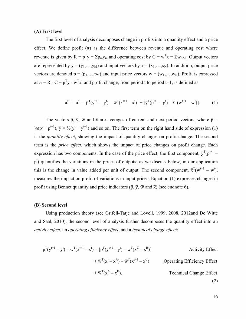
(A) First level

The first level of analysis decomposes change in profits into a quantity effect and a price

effect. We define profit (π) as the difference between revenue and operating cost where

revenue is given by R = pTy = Σpmym and operating cost by C = wTx = Σwnxn. Output vectors

are represented by y = (y1,…,yM) and input vectors by x = (x1,…,xN). In addition, output price

vectors are denoted p = (p1,…,pM) and input price vectors w = (w1,…,wN). Profit is expressed

as π = R - C = pTy - wTx, and profit change, from period t to period t+1, is defined as

πt+1 - πt = [pT(yt+1 – yt) – wT(xt+1 – xt)] + [yT(pt+1 – pt) – xT(wt+1 – wt)]. (1)

The vectors p, y, w and x are averages of current and next period vectors, where p =

½(pt + pt+1), y = ½(yt + yt+1) and so on. The first term on the right hand side of expression (1)

is the quantity effect, showing the impact of quantity changes on profit change. The second

term is the price effect, which shows the impact of price changes on profit change. Each

expression has two components. In the case of the price effect, the first component, yT(pt+1 –

pt) quantifies the variations in the prices of outputs; as we discuss below, in our application

this is the change in value added per unit of output. The second component, xT(wt+1 – wt),

measures the impact on profit of variations in input prices. Equation (1) expresses changes in

profit using Bennet quantity and price indicators (p, y, w and x) (see endnote 6).

(B) Second level

Using production theory (see Grifell-Tatjé and Lovell, 1999, 2008, 2012and De Witte

and Saal, 2010), the second level of analysis further decomposes the quantity effect into an

activity effect, an operating efficiency effect, and a technical change effect:

pT(yt+1 – yt) – wT(xt+1 – xt) = [pT(yt+1 – yt) – wT(xC – xB)] Activity Effect

+ wT(xt – xA) – wT(xt+1 – xC) Operating Efficiency Effect

+ wT(xA – xB). Technical Change Effect (2)

17

We represent the technology available at time t by that period’s production possibility

frontier Ft and it convex hull h(Ft), the set of feasible input/output combinations given Ft. See

Figure 4.

[INSERT FIGURE 4 ABOUT HERE]

Input vectors xA, xB, and xC are theoretical. Specifically, xA is the efficient amount of

input needed to produce the realized output level yt with technology Ft; xB is the efficient

amount of input needed to produce the realized output level yt with technology Ft+1; and xC is

the efficient amount of input needed to produce the realized output level yt+1 with technology

Ft+1.

[INSERT FIGURE 5 ABOUT HERE]

Figure 5 (which is for the case M = N = 1) is helpful to understand the decomposition.

The activity effect measures how much variation in profits is due to changes in sales volume

and change in the volume of inputs employed (using efficiently the latest available technology

in the retailing industry). This corresponds to a movement along the production possibility

frontier of period t+1 and is indicated by the arrow connecting operating-efficient vectors (xB,

yt) and (xC,yt+1). The activity effect contributes to or detracts from profit depending on

whether the change in outputs exceeds or falls short of the corresponding change in the

efficient quantities of inputs, with the changes being evaluated at Bennet output and input

prices,  p and w. Grifell-Tatjé and Lovell (1999) have shown that in a situation with multiple

outputs and inputs, the activity effect also reflects changes in the mixes of outputs and inputs.

The operating efficiency effect measures the change in the difference between the chosen

amount of inputs to produce the observed level of output and the efficient amount of inputs

needed to produce that level of output. To produce a cost valuation of the operating efficiency

of the firm, we multiply these differences in inputs by the Bennet input price index, w.

The technical change effect measures the change in the efficient amount of inputs

needed to produce output yt when moving from technology Ft to technology Ft+1. To produce a

monetary valuation that we can relate to the evolution of profits, we multiply the change in

18

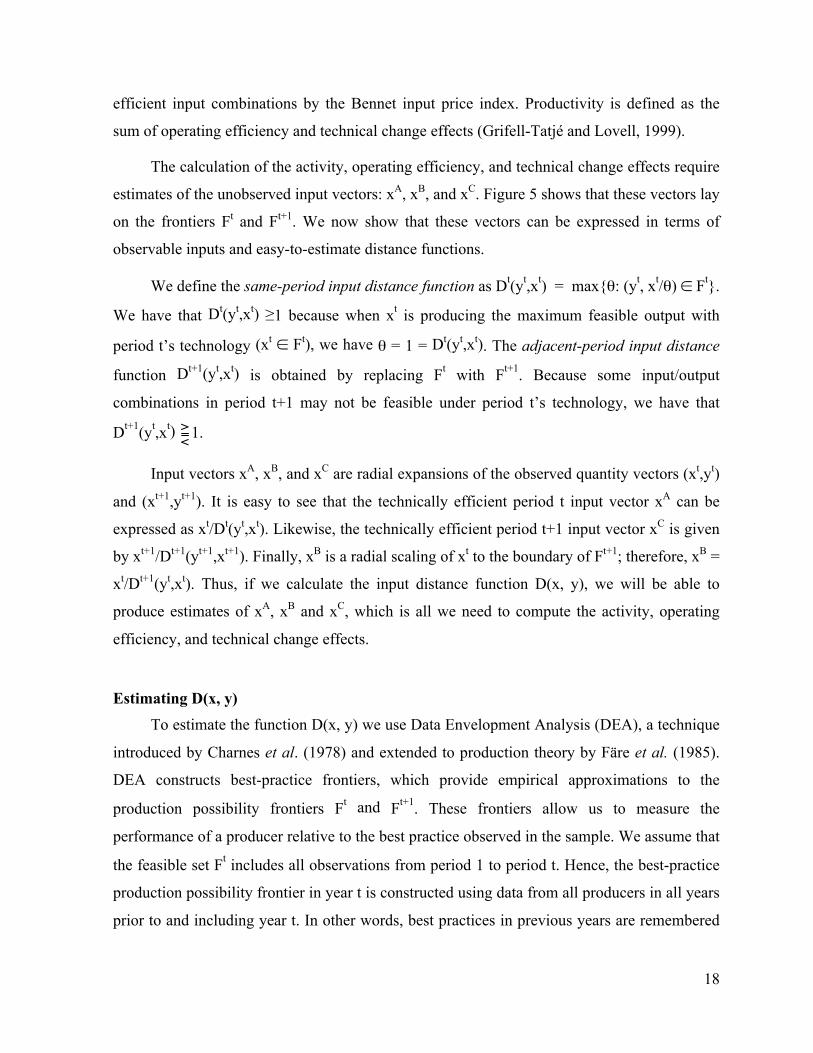
efficient input combinations by the Bennet input price index. Productivity is defined as the

sum of operating efficiency and technical change effects (Grifell-Tatjé and Lovell, 1999).

The calculation of the activity, operating efficiency, and technical change effects require

estimates of the unobserved input vectors: xA, xB, and xC. Figure 5 shows that these vectors lay

on the frontiers Ft and Ft+1. We now show that these vectors can be expressed in terms of

observable inputs and easy-to-estimate distance functions.

We define the same-period input distance function as Dt(yt,xt) = max{θ: (yt, xt/θ) ∈ Ft}.

We have that Dt(yt,xt) ≥1 because when xt is producing the maximum feasible output with

period t’s technology (xt ∈ Ft), we have θ = 1 = Dt(yt,xt). The adjacent-period input distance

function Dt+1(yt,xt) is obtained by replacing Ft with Ft+1. Because some input/output

combinations in period t+1 may not be feasible under period t’s technology, we have that

Dt+1(yt,xt) >=<1.

Input vectors xA, xB, and xC are radial expansions of the observed quantity vectors (xt,yt)

and (xt+1,yt+1). It is easy to see that the technically efficient period t input vector xA can be

expressed as xt/Dt(yt,xt). Likewise, the technically efficient period t+1 input vector xC is given

by xt+1/Dt+1(yt+1,xt+1). Finally, xB is a radial scaling of xt to the boundary of Ft+1; therefore, xB =

xt/Dt+1(yt,xt). Thus, if we calculate the input distance function D(x, y), we will be able to

produce estimates of xA, xB and xC, which is all we need to compute the activity, operating

efficiency, and technical change effects.

Estimating D(x, y) To estimate the function D(x, y) we use Data Envelopment Analysis (DEA), a technique

introduced by Charnes et al. (1978) and extended to production theory by Färe et al. (1985).

DEA constructs best-practice frontiers, which provide empirical approximations to the

production possibility frontiers Ft and Ft+1. These frontiers allow us to measure the

performance of a producer relative to the best practice observed in the sample. We assume that

the feasible set Ft includes all observations from period 1 to period t. Hence, the best-practice

production possibility frontier in year t is constructed using data from all producers in all years

prior to and including year t. In other words, best practices in previous years are remembered

19

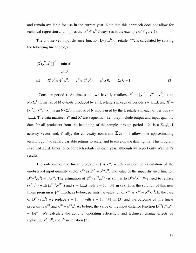
and remain available for use in the current year. Note that this approach does not allow for

technical regression and implies that xA ≧ xB always (as in the example of Figure 5).

The unobserved input distance function Dt(yt,xt) of retailer ‘o’, is calculated by solving

the following linear program:

[Dt(y

ot,x

ot)]

-1 = min φA

φA,λS

s.t Xs λs ≤ φA xot, yot ≤ Ys λs, λs ≥ 0, Σi λi = 1. (3)

Consider period t. At time s ≤ t we have Is retailers; Ys = [y

1s,...,yos,...,y

Is] is an

M×Σst=1Is matrix of M outputs produced by all Is retailers in each of periods s = 1,...,t, and X

s =

[x1s

,...,xos,...,xIs] is an N×Σs

t=1Is matrix of N inputs used by the Is retailers in each of periods s =

1,...,t. The data matrices Ys and Xs are sequential, i.e., they include output and input quantity

data for all producers from the beginning of the sample through period t; λs is a Σst=1Is×1

activity vector and, finally, the convexity constraint Σiλi = 1 allows the approximating

technology Ft to satisfy variable returns to scale, and to envelop the data tightly. This program

is solved Σst=1Is times, once for each retailer in each year, although we report only Walmart’s

results.

The outcome of the linear program (3) is φA, which enables the calculation of the

unobserved input quantity vector xoA as xoA = φoAxot. The value of the input distance function

Dt(yot,xot) = 1/φoA. The estimation of Dt+1(yt+1,xt+1) is similar to Dt(yt,xt). We need to replace

(xot,yot) with (xot+1,yot+1) and s = 1,...,t with s = 1,...,t+1 in (3). Thus the solution of this new

linear program is φoC which, as before, permits the valuation of xoC as xoC = φoCxt+1. In the case

of Dt+1(yt,xt) we replace s = 1,...,t with s = 1,...,t+1 in (3) and the outcome of this linear

program is φoB and xoB = φoBxt. As before, the value of the input distance function Dt+1(yot,xot)

= 1/φoB. We calculate the activity, operating efficiency, and technical change effects by

replacing xA, xB, and xC in equation (2).

20

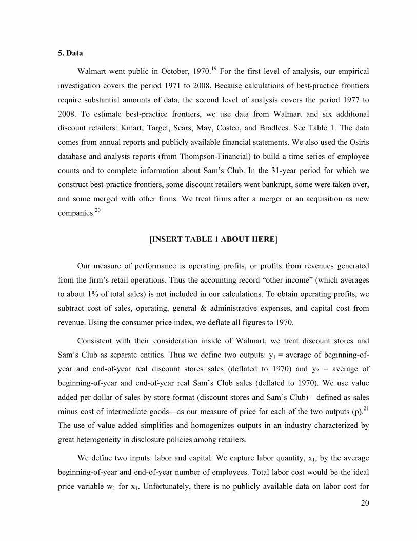
5. Data

Walmart went public in October, 1970.19 For the first level of analysis, our empirical

investigation covers the period 1971 to 2008. Because calculations of best-practice frontiers

require substantial amounts of data, the second level of analysis covers the period 1977 to

2008. To estimate best-practice frontiers, we use data from Walmart and six additional

discount retailers: Kmart, Target, Sears, May, Costco, and Bradlees. See Table 1. The data

comes from annual reports and publicly available financial statements. We also used the Osiris

database and analysts reports (from Thompson-Financial) to build a time series of employee

counts and to complete information about Sam’s Club. In the 31-year period for which we

construct best-practice frontiers, some discount retailers went bankrupt, some were taken over,

and some merged with other firms. We treat firms after a merger or an acquisition as new

companies.20

[INSERT TABLE 1 ABOUT HERE]

Our measure of performance is operating profits, or profits from revenues generated

from the firm’s retail operations. Thus the accounting record “other income” (which averages

to about 1% of total sales) is not included in our calculations. To obtain operating profits, we

subtract cost of sales, operating, general & administrative expenses, and capital cost from

revenue. Using the consumer price index, we deflate all figures to 1970.

Consistent with their consideration inside of Walmart, we treat discount stores and

Sam’s Club as separate entities. Thus we define two outputs: y1 = average of beginning-of-

year and end-of-year real discount stores sales (deflated to 1970) and y2 = average of

beginning-of-year and end-of-year real Sam’s Club sales (deflated to 1970). We use value

added per dollar of sales by store format (discount stores and Sam’s Club)—defined as sales

minus cost of intermediate goods—as our measure of price for each of the two outputs (p).21

The use of value added simplifies and homogenizes outputs in an industry characterized by

great heterogeneity in disclosure policies among retailers.

We define two inputs: labor and capital. We capture labor quantity, x1, by the average

beginning-of-year and end-of-year number of employees. Total labor cost would be the ideal

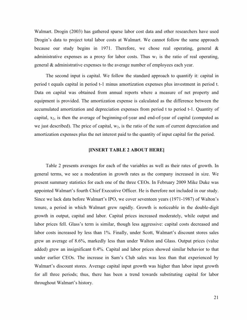
price variable w1 for x1. Unfortunately, there is no publicly available data on labor cost for

21

Walmart. Drogin (2003) has gathered sparse labor cost data and other researchers have used

Drogin’s data to project total labor costs at Walmart. We cannot follow the same approach

because our study begins in 1971. Therefore, we chose real operating, general &

administrative expenses as a proxy for labor costs. Thus w1 is the ratio of real operating,

general & administrative expenses to the average number of employees each year.

The second input is capital. We follow the standard approach to quantify it: capital in

period t equals capital in period t-1 minus amortization expenses plus investment in period t.

Data on capital was obtained from annual reports where a measure of net property and

equipment is provided. The amortization expense is calculated as the difference between the

accumulated amortization and depreciation expenses from period t to period t-1. Quantity of

capital, x2, is then the average of beginning-of-year and end-of-year of capital (computed as

we just described). The price of capital, w2, is the ratio of the sum of current depreciation and

amortization expenses plus the net interest paid to the quantity of input capital for the period.

[INSERT TABLE 2 ABOUT HERE]

Table 2 presents averages for each of the variables as well as their rates of growth. In

general terms, we see a moderation in growth rates as the company increased in size. We

present summary statistics for each one of the three CEOs. In February 2009 Mike Duke was

appointed Walmart’s fourth Chief Executive Officer. He is therefore not included in our study.

Since we lack data before Walmart’s IPO, we cover seventeen years (1971-1987) of Walton’s

tenure, a period in which Walmart grew rapidly. Growth is noticeable in the double-digit

growth in output, capital and labor. Capital prices increased moderately, while output and

labor prices fell. Glass’s term is similar, though less aggressive: capital costs decreased and

labor costs increased by less than 1%. Finally, under Scott, Walmart’s discount stores sales

grew an average of 8.6%, markedly less than under Walton and Glass. Output prices (value

added) grew an insignificant 0.4%. Capital and labor prices showed similar behavior to that

under earlier CEOs. The increase in Sam’s Club sales was less than that experienced by

Walmart’s discount stores. Average capital input growth was higher than labor input growth

for all three periods; thus, there has been a trend towards substituting capital for labor

throughout Walmart’s history.

22

6. Results

Table 3 presents our decomposition of profit variation.22 Columns 3 and 4 show the

results of the first level of analysis (equation 1), the decomposition of change in profit into

aggregated price and quantity effects. Of course, the sum of these two columns equals column

2. The results from the second level of analysis (equation 2) are shown in columns 5, 6, and 7.

There, we decompose the quantity effect into the activity, operating efficiency, and technical

change effects. These three effects add up to column 4, the quantity effect. Table 4 gives

further detail on the price effect by breaking it down by outputs and inputs. Table 5 gives

similar additional detail on the quantity effect.

In general terms we observe an increase in the values of the components of profit

change, although the series are steady. The price effect is generally negative, and the quantity

effect is positive, as expected (see the aggregate information at the end of Table 3). The

quantity effect more than compensated for the price effect, so the resulting change in profit

was positive. A closer look to the quantity effect in Table 5 reveals that the output quantity

effect grew faster than the input quantity effect. On the other hand, Table 4 shows that the

output price effect was generally negative during Walton’s and Glass’s tenure, but positive

under Scott. Capital input prices decreased, while labor prices increased (with the exception of

Walton’s years). In summary (last row of Table 4), the change in capital prices decreased costs

by $341.24 million (constant 1970 dollars) while labor prices increased costs by $1,134.84

million over the period 1972-2008. Finally, the productivity and activity effects were mostly

positive.

Sam Walton 1972-1988:

Walmart registered increasing real profits during Sam Walton’s tenure.23 The price

effect was insignificantly negative, while the quantity effect was notably positive. Table 4

reveals that the output price effect was in general negative, which implies a reduction in value

added per item sold. The input price effect was also negative, which is consistent with cost

consciousness and the human resource practices as applied by Walton. Since the price effect

is defined as the difference between output price effect and input prices effect, then for some

years the firm enjoyed positive price effects because it did not pass on all the savings obtained

by controlling costs to customers. Negative output price effects are associated with EDLP,

23

pressure over vendors, and investing in technology. It was precisely during this period when

Walmart computerized the management of inventories, deployed the UPC system, and set up

its satellite system.

The activity effect was generally positive, with the exception of the period 1983 to 1985.

A negative activity effect means, in this context, that the increase in efficient inputs costs

exceeded that of value added. This negative activity effect was compensated by a positive

productivity change in those years.

The productivity effect was initially negative due to operational inefficiencies that were

later corrected. The company enjoyed positive technical change during Walton’s last four

years. In aggregate, improvements in productivity were more important than increments in

activity levels in explaining the quantity effect. In Figure 3 we observe that five levers are

linked to the activity effect and only one to technical change. Our empirical results show that

technology was the most important lever during Walton’s years. It accounted for more than

58.20% of the change in profits. The company was not only operationally efficient but it also

innovated, and pushed outwards the boundaries of the production possibility frontier.

The year 1981 was special, as reflected in Tables 3, 4 and 5 (for the period 1980-1981).

This year Walmart made its first major acquisition: Kuhn’s Big K stores. Sam Walton made

the following statement referring to this event: “But we’d never bitten off anything close to

this size before, and we didn’t know what it would be like trying to digest it” (Walton, 1992,

p. 197). This acquisition mainly affected the output price and the price of capital. The year

1986 was also exceptional due to an increase in sales of 41% (in nominal terms). This increase

is the second largest of the complete series (the largest increase in sales occurred in 1972-1973

period).

David Glass 1988-2000: Contrary to Walton’s era, change in profit during Glass’s period was due mainly to the

activity effect. The company experienced few technological improvements and no changes in

efficiency levels (observe David Glass’s subtotal row in Table 3). When Glass left, Walmart’s

sales were 12 times greater than when Walton stepped down. The analysis reveals that Glass’s

secret of success was his emphasis in all levers related to the activity effect while keeping

24

Walmart operationally efficient. Table 5 reveals that output and input quantities were all

positive during Glass’s years. Output quantities grew faster than input quantities. In Table 4 it

can be observed that the output price effect was mainly negative (as in the case of Walton),

while the input prices of capital and labor followed different trends. Specifically, the labor

input price effect was positive (in aggregate terms), contrary to what had happened in the

previous period. Labor prices therefore increased under Glass’s administration, a result of

changes in human resource practices. On the other hand, the capital input price effect was

negative for the whole period.

As described in Section 3, David Glass pulled some business model levers differently

than Sam Walton. Glass discontinued the “Buy American” campaign, opening the doors to

overseas suppliers. He also spurred the expansion of the company by deploying new retail

formats and building new stores in the U.S. and abroad. The main difference between Walton

and Glass was in the decomposition of the quantity effect. Walton’s years were characterized

by the importance of technology, while in Glass’s years the main component was the activity

effect. Another difference comes from the fact that in Glass’s last years, output prices effect

increased (the only exception being the last year of Glass’s tenure).24

Three years (1991, 1995, and 1997) deserve separate discussion. In 1991, the price

effect decreased substantially (although the activity effect more than compensated for it). In

December 1990, Walmart completed the acquisition of McLane (a company that provided and

distributed goods to different retail stores, including Walmart). Also at that time, Walmart was

fully deploying Sam’s Club nationwide.25 Both Sam’s Club and McLane had lower markups

than Walmart. This explains why the value added of the company decreased substantially in

1991. The strong positive activity effect in 1991 is explained by the fact that Sam’s Club and

McLane had higher sales volumes relative to the amount of inputs used. Sam’s Club was a no-

frills store where items were sold in bulk.

Walmart had a difficult year in 1995. In prior years, sales were growing at rates greater

than 20% but in 1995 the growth rate was only 13%. The company was investing heavily

outside the U.S. with mixed results. Sam’s Club was not performing as expected. In 1993 the

warehouse franchise registered $14.7 billion in sales (current dollars), one year later that

figure was $19 billion; in 1995, Sam’s Club reported $19.068 billion in sales. The growth rate

25

was below inflation. Walmart’s 1996 annual report states that the company was refocusing

Sam’s Club strategy. However, Table 5 reveals that the output quantity effect for Sam’s Club

never recovered the growth levels prior to 1995.

The price effect became positive after 1997. Table 4 reveals that the output price effect

(which used to be negative) was positive at that time. Several systems that improved inventory

management and a change in the merchandise mix were implemented during those years and

these improvements reduced the cost of sales.26 Despite Walmart obtaining higher value added

per dollar sold, the activity effect remained strong although smaller than in previous years.

Lee Scott 2000-2008:

Scott’s tenure was characterized by a moderation in growth rates. Walmart’s profit

increased not only because of changes in activity levels, but also because of productivity

improvements due to technical change (see subtotal in Table 3). The company enjoyed

substantial technical progress and the price effect had a similar negative impact as in the

previous period. Nevertheless, the output price effect (Table 4) changed sign, becoming

positive. This result signals a laxer implementation of EDLP. However, the labor input price

effect was the component that showed the most striking shift. Labor prices increased

significantly during this period. Company records relate increases to insurance and payroll-

related costs.27 Our analysis indicates that out of all the levers “pulled differently” by Lee

Scott as described in Section 3, it was changes in human resource practices that had the largest

effect on Walmart’s performance.

Table 5 reveals that the importance of Sam’s Club (in terms of contribution to profits)

diminished during this time. Under Glass’s administration, Sam’s Club contributed $820

million to profits. Under Scott’s tenure, it was only $392.9 million. The company applied

different measures to mend Sam’s performance but, these polices did not deliver the desired

results.

The year 2003 deserves separate analysis. McLane was sold that year for $1.5 billion

and the company recorded extraordinary income of $151 million after taxes. Walmart sold

McLane because it did not fit with its core business. McLane sales in 2002 were $14.9 billion,

26

so its influence on the company’s financials was substantial. The components of profit change

most affected by this sale were output quantities and prices.

The last year of the series shows negative change in real profits. In current dollars,

Walmart registered an increase in profits. However, profit grew less than inflation. The main

reason for the poor performance was a disappointing year for Sam’s Club and the negative

impact of the exchange rate for international operations.

Scott followed the lead of Walton and Glass. By 2000, however, Walmart was no longer

invisible. It was a giant charged with underpaying workers and other questionable aggressive

practices. Abroad, the company found able competitors that emulated its strategy. Scott had to

manage Walmart in a much more hostile and difficult environment than his antecessors. When

Walton was leading, Kmart was the rival to beat. Under Scott, Walmart became the target.

7. Conclusions

The aim of this paper has been to contribute to the extant literature on business models.

We have argued that business models are composed of levers and that a central task of the top

management team is to choose on how to configure (i.e., pull) each lever. Part of the reason

why we often observe heterogeneity of performance of companies with similar business

models is that management has chosen to configure business model levers differently. Overall,

our analysis suggests that the effectiveness of a particular business model depends not only on

its design (what levers are part of the business model) but, most importantly, on its

implementation (how each lever is configured).

The literature is rich in theoretical frameworks that help analysts describe business

models qualitatively, but little progress has been made in developing micro-founded methods

to quantify business model performance. Ours is a first step in this direction. The method we

propose provides a clear assessment of the impact of a company’s choices on profits. We rely

on theory of index numbers and production theory. Production theory provides the

fundamentals required to define and quantify concepts central to strategy such as productivity,

technical change, or operating efficiency in the context of economic performance assessment.

These are linked to consequences of firm choices and are naturally used as explanatory

variables of profit change, our measure of performance. One strength of our approach is that

27

we do not assume that firms maximize profits as none of our derivations relies on this

assumption (which is controversial in strategy).

Books, journal articles, case studies, and TV documentaries have presented diverse

descriptions for how from humble beginnings Sam Walton built Walmart, the world’s most

successful discount retailer. We have constructed a business model representation based on

these sources as well as information published by the company, and have quantified the effect

of business model choices by the first three CEOs on Walmart’s performance.

Overall, we have found that the price effect has been mostly negative but the quantity

effect has been positive. Essentially, the company grew by selling more goods at very low

prices. Under Sam Walton, investments in technology and improvements in efficiency had the

largest effect on Walmart’s profit growth. With David Glass, it was increases in activity

levels: the firm created a vast network of discount stores, supercenters and neighborhood

markets in the U.S. and abroad to reach ever-larger numbers of consumers, it expanded its

selection of goods by including groceries in its stores, and exerted pressure over its vendors

which allowed the company to reduce prices and boost sales volume. In more recent years,

Walmart’s human resource practices were the target of criticism which put pressure on Lee

Scott to raise salaries and improve benefits to associates.

One important limitation of our analysis is that although we have included Walmart’s

competitors in building the production possibility frontier, we have not considered explicitly

the effects of interactions with competitors on Walmart’s profitability over time. For

tractability reasons, we have not looked at explicit interactions between competitors and we

leave this issue for further research. However, we should also say that the fact that Walmart

chose to operate in dispersed, rural locations also meant that it interacted less with other

discount retailers. Walton acknowledged in his memoirs that this strategy shielded Walmart

from competition.

Our research has revealed that in the years 1971 to 2008 Walmart’s business model

remained that of a traditional discount retailer. While the first three CEOs pulled Walmart’s

business model levers differently, these did not change. Perhaps the most important challenge

currently faced by Michael Duke (CEO since 2009) is deciding whether to continue Walmart’s

traditional business model (and consider pulling levers differently) or to come up with a

28

different, original set of levers that fundamentally redefines what it means to compete in

discount retail. For example, how important should the online channel be to Walmart and what

should the company do to have a competitive advantage in that space? Or should Walmart be

active in banking and provide credit to customers and suppliers? Or should Walmart’s adopt

elements of multi-sided platforms in addition to those of a merchant? It is our hope that the

method that we have presented in this paper can help inform attempts by the company to

innovate in its business model and to quantify the effects of such innovations.

References

Amit, R., & Zott, C. (2001). “Value creation in e-business.” Strategic Management Journal, 22, 493-520.

Baden-Fuller, C., I. MacMillan, B. Demil, X. Lecocq. (2008). “Special Issue Call for Papers: Business Models.” Long Range Planning.

Balk, B. M. (2008). “Searching for the holy grail of index number theory.” Journal of Economic and Social Measurement 33(1), 19-25.

Barbaro, M., & Gills, J. (2005). “Wal-Mart at The Forefront of The Hurricane Relieve”. Washington Post. September 6.

Barney, J. (1991). “Firm resources and sustained competitive advantage.” Journal of Management, 17(1), 99-120.

Basker, E. & Pham Hoang, V. (2008). “Wal-Mart as a catalyst to US-China trade.” Working Paper: Available at SSRN: http://ssrn.com/abstract=987583

Basker, E. (2005). “Selling a cheaper mousetrap: Wal-Mart’s effect on retail prices.” Journal of Urban Economics 58(2), 203-229.

_______ (2005b). “Job creation or destruction? Labor Market Effects of Wal-Mart Expansion.” Review of Economics and Statistics, 87(1), 174-183.

Basker, E., & Noel, M. (2007). “The Evolving Food Chain: Competitive Effects of Wal-Mart’s Entry into The Supermarket Industry.” Journal of Economics and Management Strategy, 18(4), 977-1009.

Basker, E., Klimek, S., & Pham Hoang, V. (2008). “Supersize it: The growth of retail chains and the rise of the 'big box' retail format.” Department of Economics, University of Missouri, Working Papers: 0809.

Bennet, T. L. (1920). “The theory of measurement of changes in cost of living.” Journal of the Royal Statistical Society, 83, 455–462.

Bonacich, E., & Wilson, J. (2006). “Global Production and Distribution: Wal-Mart’s Global Logistics Empire (with Special Reference to The China / Southern California Connection).” In S. D. Brunn (Ed.), Wal-Mart World (2006). New York: Routledge Taylor & Francis Group.

29

Boussemart, J.-Ph., Demil, B., Deville, A., La Villarmois, O., Lecocq, X., Leleu, H. (2012). “Explaining the Profit Differential between Two Firms.” Working Paper. University of Lille 3 and IÉSEG School of Management.

Bradley, S. & Ghemawat P. (2002) “Wal*Mart stores, inc.” Harvard Business School. Case 794-024.

Brandenburger, A. & Stuart H. W. (1996) “Value-Based Business Strategy” Journal of Economics & Management Strategy, 5(1), 5-24.

Burt, S., & Sparks, L. (2006). “ASDA: Wal-Mart in the United Kingdom.” Wal-Mart World (2006). New York: Routledge Taylor & Francis Group.

Casadesus-Masanell, R., & Feng Zhu (2010). “Strategies to fight ad-sponsored rivals.” Management Science, 56(9), 1484-1499.

Casadesus-Masanell, R., & Larson, T. (2009). “Competing through business models (D).” Harvard Business School, Case 710-410.

Casadesus-Masanell, R., & Ricart, J. E. (2008). “Competing through business models (A).” Harvard Business School, Case 708-452.

_________, ________. (2010). “From strategy to business model and onto tactics.” Special Issue on Business Models, Long Range Planning 43(2), 195-215.

_________, ________. (2011). “How to Design a Winning Business Model.” Harvard Business Review 89(1-2), 100-107.

Caves, D. W., Christensen, L. R., & Diewert, W. E. (1982). “The economic theory of index numbers and the measurement of input, output, and productivity.” Econometrica, 50(6), 1393-1414.

Charnes, A., Cooper, W. W., & Rhodes, E. (1978). “Measuring the efficiency of decision making units.” European Journal of Operational Research, 2(6), 429-444.

Chesbrough, H., & Rosenbloom, R. (2002). “The role of the business model in capturing value from innovation: evidence from Xerox corporation’s technology spin-off companies.” Industrial and Corporate Change, 11(3), 529-555.

Cyert, R.M. and Hedrick, L.H. (1972), “The theory of the firm: past, present and future; an interpretation,” Journal of Economic Literature 10(2), 398-412.

Davis, H. S. (1955), Productivity Accounting. Philadelphia: University of Pennsylvania Press. De Witte, K., and D. S. Saal (2010), “Is a Little Sunshine All We Need? On the Impact of

Sunshine Regulation on Profits, Productivity and Prices in the Dutch Drinking Water Sector,” forthcoming Journal of Regulatory Economics.

Diewert, W. E. (2005). “Index number theory using differences rather than ratios.” American Journal of Economics and Sociology, 64(1), 347–395.

Drogin, R. (2003). “Statistical analysis of gender Patterns in Wal-Mart workforce.” Dube, A., & Jacobs, K. (2004). “Hidden cost of Wal-Mart jobs use of safety net programs by

Wal-Mart workers in California.” University of California-Berkeley, Labor Center. Unpublished paper.

Dube, A., & Wertheim, S. (2005). “Wal-Mart and job quality-what do we know, and should we care?” Prepared for Presentation at Center for American Progress,

30

Dunnett, J., & Arnold, S. J. (2006). Falling prices, happy faces: organizational culture at Wal-Mart. Wal-mart world (). New York: Routledge Taylor & Francis Group.

Eilon, S,. B. Gold and J. Soesan (1976), “An Integrated Steel Plant,” in (Ed. Eilon, S,. B. Eilon, S., B. Gold and J. Soesan (1975), “A Productivity Study in a Chemical Plant,” Omega

3:3, 329-43. Färe, R., S. Grosskopf, B. Lindgren and P. Roos (1994). Productivity developments in

Swedish hospitals: a Malmquist output index approach. Data Envelopment Analysis: Theory, Methodology and Applications. Boston: Kluwer Academic Publishers.

Färe, R., S. GrossKopf and C.A.K. Lovell (1985). “The Measurement of Efficiency of Production.” Kluwer-Nijhoff Publishing: Boston-Dordrecht-Lancaster.

Fisher, I. (1911). “The purchasing power of money,” Reprinted 1971 by Augustus M. Kelley Publishers: New York.

Fishman, C. (2006). The Wal-Mart effect. New York: The Penguin Press. Genescà-Garrigosa, E. & Grifell-Tatjé, E. (1992),” "Profits and Total Factor Productivity: A

Comparative Analysis," Omega. The International Journal of Management Science, 20(5/6), 553-568.

Ghemawat, P. (1989). “Wal-Mart Stores' Discount Operations.” Harvard Business School. Case 387-018

Ghemawat, P., Mark, K., & Bradley, S. P. (2004). “Wal-Mart Stores in 2003.” Harvard Business School. Case 704-430.

Gilchrist, R.R., (1971). “Managing for Profit. The Added Value Concept.” London: George Allen and Unwin LTD.

Global Insight Inc., (2005). The Economic Impact of Wal-Mart. Gold, B. (1971). Explorations in Managerial Economics. Productivity, Costs, Technology and

Growth. Basic Books Inc: New York. Graff, T. O. (1998). “The locations of Wal-Mart and Kmart supercenters: contrasting

corporate strategies.” Professional Geographer, 50(1), 46-57. Graff, T. O. and Ashton D. (1994) “Spatial diffusion of Wal-Mart: contagious and reverse

hierarchical elements.” Professional Geographer, 46(1), 19-29. Grifell-Tatje, E., & Lovell, C. A. K. (1995). “A note on the Malmquist Productivity Index.”

Economic Letters, 47(2), 169-175. _________, ________. (1999). “Profits and productivity.” Management Science, 45(9), 1177-

1193. _________, ________. (2008). “Productivity at the post: its drivers and its distribution.”

Journal of Regulatory Economics, 33(2), 133-158. _________, ________. (2012). “The Economics of Business Performance,” forthcoming

Cambridge University Press. Hausman, J., & Leibtag, E. (2007). “Consumer benefits from increased competition in

shopping outlets: measuring the effect of Wal-Mart.” Journal of Applied Econometrics, 22(7), 1157-1177.

Hedman, J., & Kalling, T. (2003). “The Business Model Concept: Theoretical Underpinnings and Empirical Illustrations.” European Journal of Information Systems, 12(1), 49.

31

Holmes, T. (2008). “The diffusion of Wal-Mart and economies of density.” NBER Working Paper: 13783.

Jia, P. (2008). “What Happens When Wal-Mart Comes To Town: An Empirical Analysis Of The Discount Retailing Industry.” Econometrica, 76(6), 1263-1316.

Johnson, H. T. (1975), “Management Accounting in an Early Integrated Industrial: E. I. DuPont de Nemours Powder Company, 1903-1912,” Business History Review 49:2 (Summer), 184-204.

________ (1978). “Management Accounting in an Early Multidivisional Organization: General Motors in the 1920s,” Business History Review 52:4 (Winter), 490-517.

Kendrick, J., & Creamer, D. (1961). Measuring Company Productivity: A Handbook with Case Studies. New York: Conference Board.

Kurosawa, K. (1975). “An Aggregate Index for the Analysis of Productivity and Profitability,” Omega. The International Journal of Management Science 3:2, 157-68.

___________ (1991), Productivity Measurement and Management at the Company Level: The Japanese Experience. Amsterdam: Elsevier.

Lecocq, X., Demil, B., & Ventura, J. (2010). “Business model as a research program in strategic management: an appraisal based on Lakatos.” M@n@gment, 13(4), 214-225.

Lecocq, X. Demil, B., & Warnier, V. (2006). “Le Business Model, un Outil d’Analyse Strategique,” L’Expansion Management Review, 123, 50-59.

Magretta, J. (2002). “Why business models matter.” Harvard Business Review. Mäkinen, S., & Seppänen, M. (2007). “Assessing business models with taxonomical research

criteria.” Management Research News, 30(10), 735-748. Malmquist, S. (1953). “Index numbers and indifference surfaces.” Trabajos De Estadística,

4(2), 209-242. Miller, D. M. (1984). “Profitability = Productivity + Price Recovery,” Harvard Business

Review 62:3 (May/June), 145-53. Miller, D.M., & Rao, P.M., (1989). “Analysis of profit-linked total factor productivity

measurement models at firm level,” Management Science, 35(6), 757-767. Morris, M., Schindehutte, M., & Allen, J. (2005). “The entrepreneur's business model: toward

a unified perspective.” Journal of Business Research, 58(6), 726-735. Nissim, D., and S. H. Penman (2001), “Ratio Analysis and Equity Valuation: From Research

to Practice,” Review of Accounting Studies 6:1 (March), 109-54. Oberholzer-Gee, F. (2006). “Wal-Mart's Business Environment.” Harvard Business School.

Case 706-453. Porter, M. (1980). The competitive strategy, techniques for analyzing industries and

competitors. New York: The Free Press. ________ (1985). Competitive advantage, creating and sustaining a superior performance.

New York: The Free Press. ________ (1996). “What Is Strategy?” Harvard Business Review, Nov. Dec., 61-78. ________ (2001). “Strategy and the Internet.” Harvard Business Review. Vol. 79, No. 3,

March. 63-78.

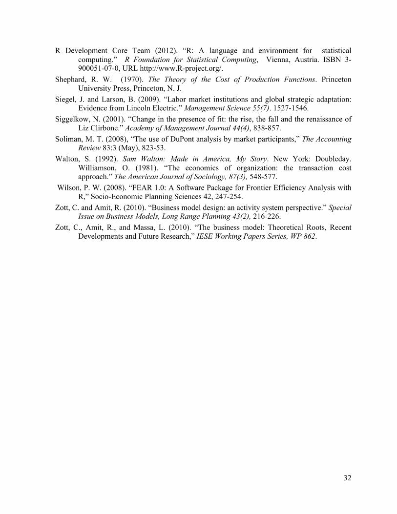
32

R Development Core Team (2012). “R: A language and environment for statistical computing.” R Foundation for Statistical Computing, Vienna, Austria. ISBN 3-900051-07-0, URL http://www.R-project.org/.

Shephard, R. W. (1970). The Theory of the Cost of Production Functions. Princeton University Press, Princeton, N. J.

Siegel, J. and Larson, B. (2009). “Labor market institutions and global strategic adaptation: Evidence from Lincoln Electric.” Management Science 55(7). 1527-1546.

Siggelkow, N. (2001). “Change in the presence of fit: the rise, the fall and the renaissance of Liz Clirbone.” Academy of Management Journal 44(4), 838-857.

Soliman, M. T. (2008), “The use of DuPont analysis by market participants,” The Accounting Review 83:3 (May), 823-53.

Walton, S. (1992). Sam Walton: Made in America, My Story. New York: Doubleday. Williamson, O. (1981). “The economics of organization: the transaction cost approach.” The American Journal of Sociology, 87(3), 548-577.

Wilson, P. W. (2008). “FEAR 1.0: A Software Package for Frontier Efficiency Analysis with R,” Socio-Economic Planning Sciences 42, 247-254.

Zott, C. and Amit, R. (2010). “Business model design: an activity system perspective.” Special Issue on Business Models, Long Range Planning 43(2), 216-226.

Zott, C., Amit, R., and Massa, L. (2010). “The business model: Theoretical Roots, Recent Developments and Future Research,” IESE Working Papers Series, WP 862.

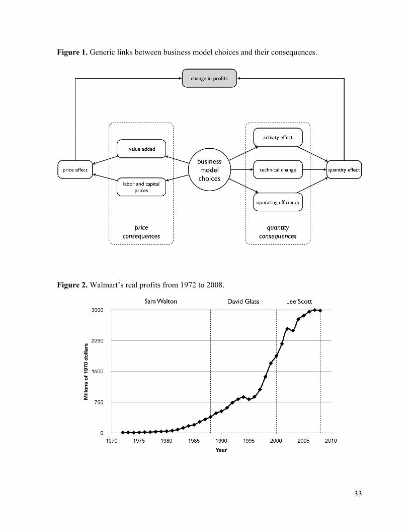
33

Figure 1. Generic links between business model choices and their consequences.

Figure 2. Walmart’s real profits from 1972 to 2008.

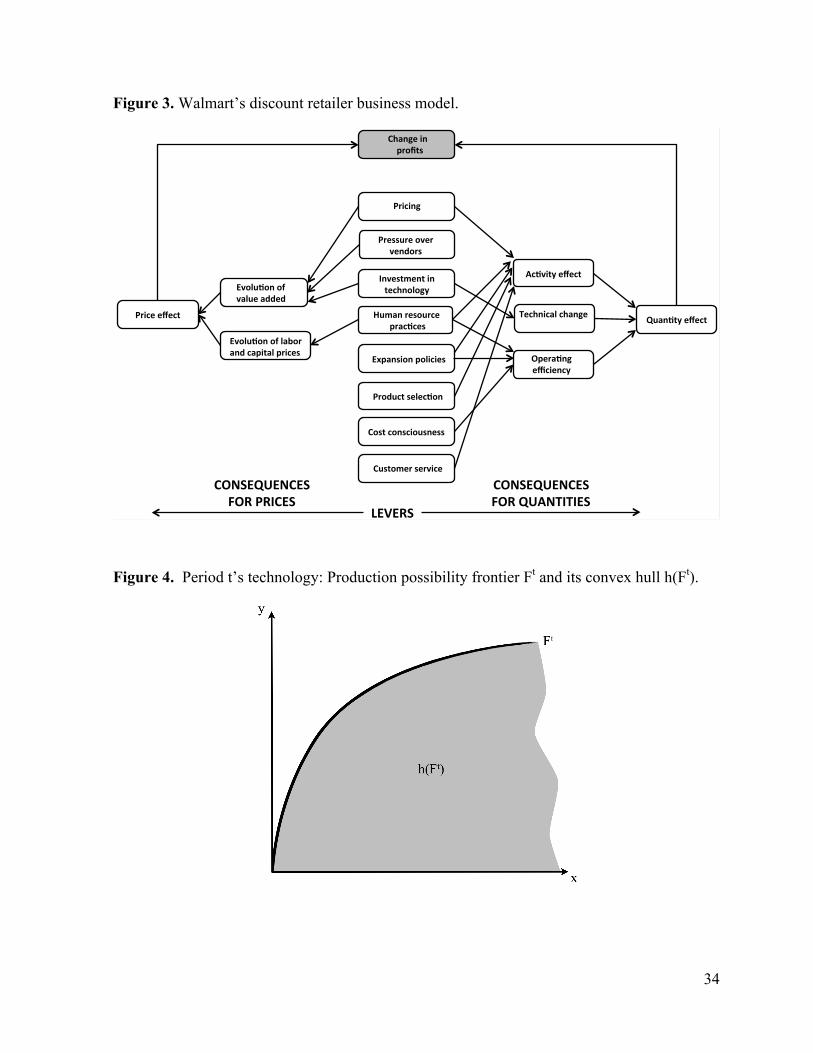
34

Figure 3. Walmart’s discount retailer business model.

Figure 4. Period t’s technology: Production possibility frontier Ft and its convex hull h(Ft).

!!!Change!in!!!!!!!!!profits!

Evolu3on!of!value!added!

Price!effect! Human!resource!!prac3ces!

Investment!in!technology!

Pressure!over!vendors!

Expansion!policies!

Product!selec3on!

Pricing!

Opera3ng!efficiency!

Technical!change!

Ac3vity!effect!

Quan3ty!effect!Evolu3on!of!labor!and!capital!prices!

LEVERS!

CONSEQUENCES!!FOR!PRICES!

CONSEQUENCES!!FOR!QUANTITIES!

Cost!consciousness!

Customer!service!

35

Figure 5. Decomposition of quantity effect for the case M = N = 1.

The activity effect is captured by the arrow connecting (xB,yt) and (xC,yt+1).

The operating efficiency effect is proportional to the difference between the distance from (xt,yt) to (xA,yt) and the distance from (xt+1,yt+1) to (xC,yt+1).

The technical change effect is represented by the arrow connecting (xA,yt) and (xB,yt).

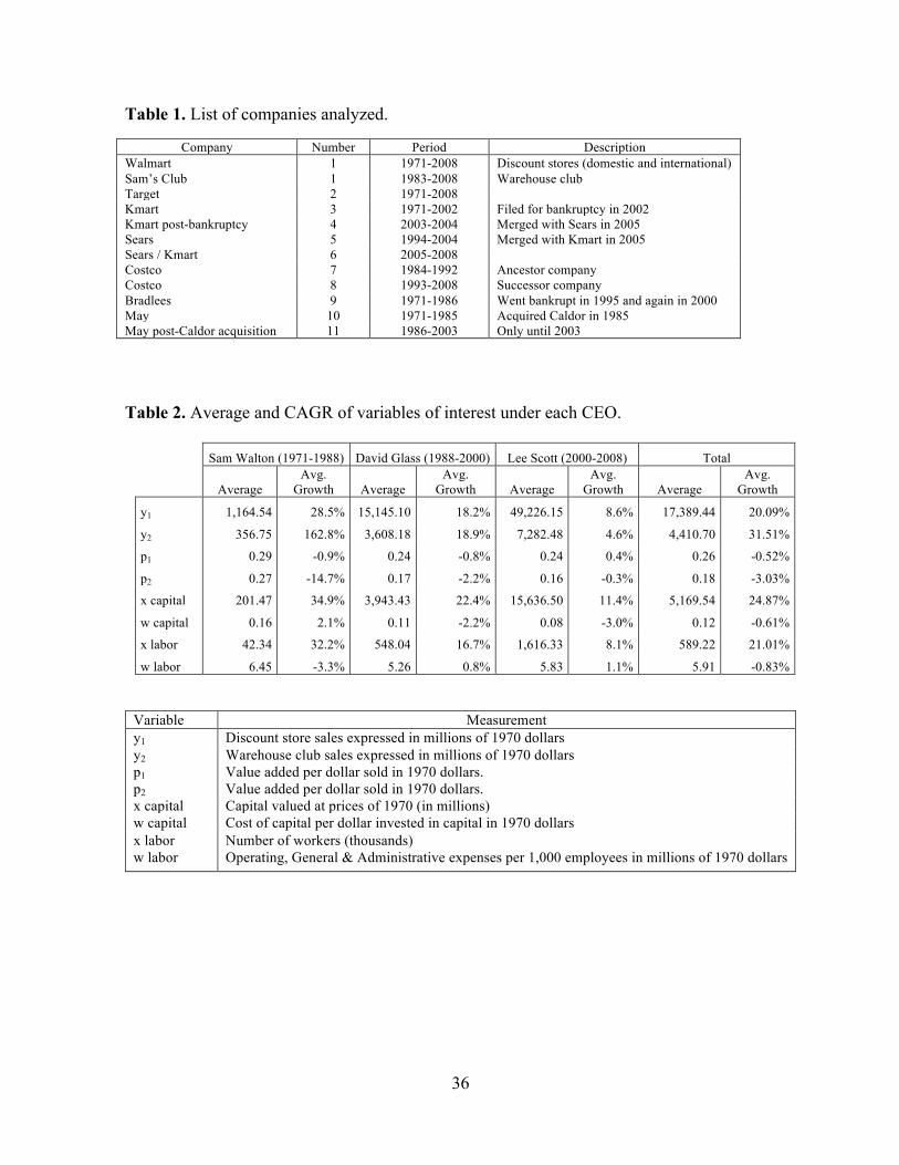
36

Table 1. List of companies analyzed.

Company Number Period Description Walmart 1 1971-2008 Discount stores (domestic and international) Sam’s Club 1 1983-2008 Warehouse club Target 2 1971-2008 Kmart 3 1971-2002 Filed for bankruptcy in 2002 Kmart post-bankruptcy 4 2003-2004 Merged with Sears in 2005 Sears 5 1994-2004 Merged with Kmart in 2005 Sears / Kmart 6 2005-2008 Costco 7 1984-1992 Ancestor company Costco 8 1993-2008 Successor company Bradlees 9 1971-1986 Went bankrupt in 1995 and again in 2000 May 10 1971-1985 Acquired Caldor in 1985 May post-Caldor acquisition 11 1986-2003 Only until 2003

Table 2. Average and CAGR of variables of interest under each CEO.

Sam Walton (1971-1988) David Glass (1988-2000) Lee Scott (2000-2008) Total

Average

Avg. Growth Average

Avg. Growth Average

Avg. Growth Average

Avg. Growth

y1 1,164.54 28.5% 15,145.10 18.2% 49,226.15 8.6% 17,389.44 20.09%

y2 356.75 162.8% 3,608.18 18.9% 7,282.48 4.6% 4,410.70 31.51%

p1 0.29 -0.9% 0.24 -0.8% 0.24 0.4% 0.26 -0.52%

p2 0.27 -14.7% 0.17 -2.2% 0.16 -0.3% 0.18 -3.03%

x capital 201.47 34.9% 3,943.43 22.4% 15,636.50 11.4% 5,169.54 24.87%

w capital 0.16 2.1% 0.11 -2.2% 0.08 -3.0% 0.12 -0.61%

x labor 42.34 32.2% 548.04 16.7% 1,616.33 8.1% 589.22 21.01%

w labor 6.45 -3.3% 5.26 0.8% 5.83 1.1% 5.91 -0.83%

Variable Measurement y1 Discount store sales expressed in millions of 1970 dollars y2 Warehouse club sales expressed in millions of 1970 dollars p1 Value added per dollar sold in 1970 dollars. p2 Value added per dollar sold in 1970 dollars. x capital Capital valued at prices of 1970 (in millions) w capital Cost of capital per dollar invested in capital in 1970 dollars x labor Number of workers (thousands) w labor Operating, General & Administrative expenses per 1,000 employees in millions of 1970 dollars

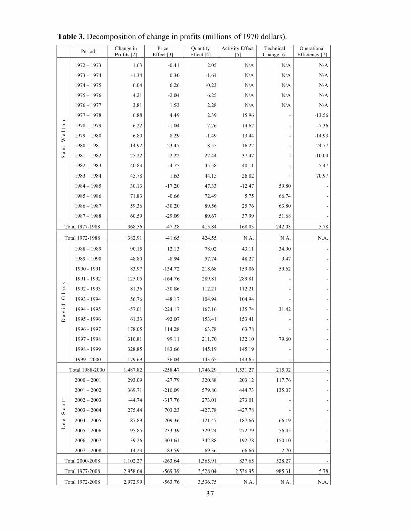
37

Table 3. Decomposition of change in profits (millions of 1970 dollars). Period Change in

Profits [2] Price

Effect [3] Quantity Effect [4]

Activity Effect [5]

Technical Change [6]

Operational Efficiency [7]

Sa

m W

alt

on

1972 – 1973 1.63 -0.41 2.05 N/A N/A N/A

1973 – 1974 -1.34 0.30 -1.64 N/A N/A N/A

1974 – 1975 6.04 6.26 -0.23 N/A N/A N/A

1975 – 1976 4.21 -2.04 6.25 N/A N/A N/A

1976 – 1977 3.81 1.53 2.28 N/A N/A N/A

1977 – 1978 6.88 4.49 2.39 15.96 - -13.56

1978 – 1979 6.22 -1.04 7.26 14.62 - -7.36

1979 – 1980 6.80 8.29 -1.49 13.44 - -14.93

1980 – 1981 14.92 23.47 -8.55 16.22 - -24.77

1981 – 1982 25.22 -2.22 27.44 37.47 - -10.04

1982 – 1983 40.83 -4.75 45.58 40.11 - 5.47

1983 – 1984 45.78 1.63 44.15 -26.82 - 70.97

1984 – 1985 30.13 -17.20 47.33 -12.47 59.80 -

1985 – 1986 71.83 -0.66 72.49 5.75 66.74 -

1986 – 1987 59.36 -30.20 89.56 25.76 63.80 -

1987 – 1988 60.59 -29.09 89.67 37.99 51.68 -

Total 1977-1988 368.56 -47.28 415.84 168.03 242.03 5.78

Total 1972-1988 382.91 -41.65 424.55 N.A. N.A. N.A.

Da

vid

Gla

ss

1988 – 1989 90.15 12.13 78.02 43.11 34.90 -

1989 – 1990 48.80 -8.94 57.74 48.27 9.47 -

1990 - 1991 83.97 -134.72 218.68 159.06 59.62 -

1991 - 1992 125.05 -164.76 289.81 289.81 - -

1992 - 1993 81.36 -30.86 112.21 112.21 - -

1993 - 1994 56.76 -48.17 104.94 104.94 - -

1994 - 1995 -57.01 -224.17 167.16 135.74 31.42 -

1995 - 1996 61.33 -92.07 153.41 153.41 - -

1996 - 1997 178.05 114.28 63.78 63.78 - -

1997 - 1998 310.81 99.11 211.70 132.10 79.60 -

1998 - 1999 328.85 183.66 145.19 145.19 - -

1999 - 2000 179.69 36.04 143.65 143.65 - -

Total 1988-2000 1,487.82 -258.47 1,746.29 1,531.27 215.02 -

Le

e S

co

tt

2000 – 2001 293.09 -27.79 320.88 203.12 117.76 -

2001 – 2002 369.71 -210.09 579.80 444.73 135.07 -

2002 – 2003 -44.74 -317.76 273.01 273.01 - -

2003 – 2004 275.44 703.23 -427.78 -427.78 - -

2004 – 2005 87.89 209.36 -121.47 -187.66 66.19 -

2005 – 2006 95.85 -233.39 329.24 272.79 56.45 -

2006 – 2007 39.26 -303.61 342.88 192.78 150.10 -

2007 – 2008 -14.23 -83.59 69.36 66.66 2.70 -

Total 2000-2008 1,102.27 -263.64 1,365.91 837.65 528.27 -

Total 1977-2008 2,958.64 -569.39 3,528.04 2,536.95 985.31 5.78

Total 1972-2008 2,972.99 -563.76 3,536.75 N.A. N.A. N.A.

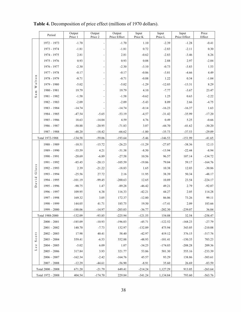
38

Table 4. Decomposition of price effect (millions of 1970 dollars).

Period Output Price 1

Output Price 2

Output Price Effect

Input Price K

Input Price L

Input Price Effect

Price Effect

Sa

m W

alt

on

1972 – 1973 -1.70 - -1.70 1.10 -2.39 -1.28 -0.41

1973 - 1974 -1.81 - -1.81 0.72 -2.83 -2.11 0.30

1974 - 1975 2.81 - 2.81 -0.62 -2.83 -3.46 6.26

1975 - 1976 0.93 - 0.93 0.08 2.88 2.97 -2.04

1976 - 1977 -2.30 - -2.30 -3.10 -0.73 -3.83 1.53

1977 - 1978 -0.17 - -0.17 -0.86 -3.81 -4.66 4.49

1978 - 1979 -0.71 - -0.71 -0.88 1.22 0.34 -1.04

1979 - 1980 -5.02 - -5.02 -1.29 -12.03 -13.31 8.29

1980 - 1981 19.79 - 19.79 4.10 -7.77 -3.67 23.47

1981 – 1982 -1.58 - -1.58 -0.62 1.25 0.63 -2.22

1982 – 1983 -2.09 - -2.09 -5.43 8.09 2.66 -4.75

1983 – 1984 -14.74 - -14.74 -0.14 -16.23 -16.37 1.63

1984 – 1985 -47.54 -5.65 -53.19 -4.57 -31.42 -35.99 -17.20

1985 – 1986 18.63 -14.04 4.59 4.76 0.49 5.25 -0.66

1986 – 1987 -50.88 -20.95 -71.83 3.07 -44.70 -41.62 -30.20

1987 – 1988 -48.20 -18.42 -66.62 -1.80 -35.73 -37.53 -29.09

Total 1972-1988 -134.58 -59.06 -193.64 -5.46 -146.53 -151.99 -41.65

Da

vid

Gla

ss

1988 – 1989 -10.51 -15.72 -26.23 -11.29 -27.07 -38.36 12.13

1989 – 1990 -35.59 4.21 -31.38 -8.50 -13.94 -22.44 -8.94

1990 – 1991 -20.69 -6.89 -27.58 10.56 96.57 107.14 -134.72

1991 – 1992 -85.45 -20.13 -105.59 -19.86 79.04 59.17 -164.76

1992 – 1993 2.39 -21.22 -18.83 1.65 10.38 12.03 -30.86

1993 – 1994 -25.56 27.72 2.16 11.95 38.39 50.34 -48.17

1994 – 1995 -101.19 -99.45 -200.63 12.65 10.89 23.54 -224.17

1995 – 1996 -90.75 1.47 -89.28 -46.42 49.21 2.79 -92.07

1996 – 1997 109.95 6.38 116.33 -42.21 44.27 2.05 114.28

1997 – 1998 169.32 3.05 172.37 -12.80 86.06 73.26 99.11

1998 – 1999 144.05 41.71 185.75 19.50 -17.41 2.09 183.66

1999 – 2000 -188.06 -14.97 -203.03 -36.77 -202.30 -239.07 36.04

Total 1988-2000 -132.09 -93.85 -225.94 -121.55 154.08 32.54 -258.47

Le

e S

co

tt

2000 – 2001 -185.09 -10.93 -196.03 -45.71 -122.52 -168.23 -27.79

2001 – 2002 140.70 -7.73 132.97 -132.89 475.94 343.05 -210.08

2002 – 2003 17.98 40.41 58.40 -42.97 419.12 376.15 -317.76

2003 – 2004 559.41 -6.53 552.88 -48.93 -101.41 -150.35 703.23

2004 – 2005 -5.02 6.09 1.07 -34.25 -174.03 -208.28 209.36

2005 – 2006 317.84 3.93 321.77 53.86 501.30 555.16 -233.39

2006 – 2007 -162.34 -2.42 -164.76 45.57 93.29 138.86 -303.61

2007 – 2008 -12.29 -44.61 -56.90 -8.91 35.60 26.69 -83.59

Total 2000 – 2008 671.20 -21.79 649.41 -214.24 1,127.29 913.05 -263.64

Total 1972 – 2008 404.54 -174.70 229.84 -341.24 1,134.84 793.60 -563.76

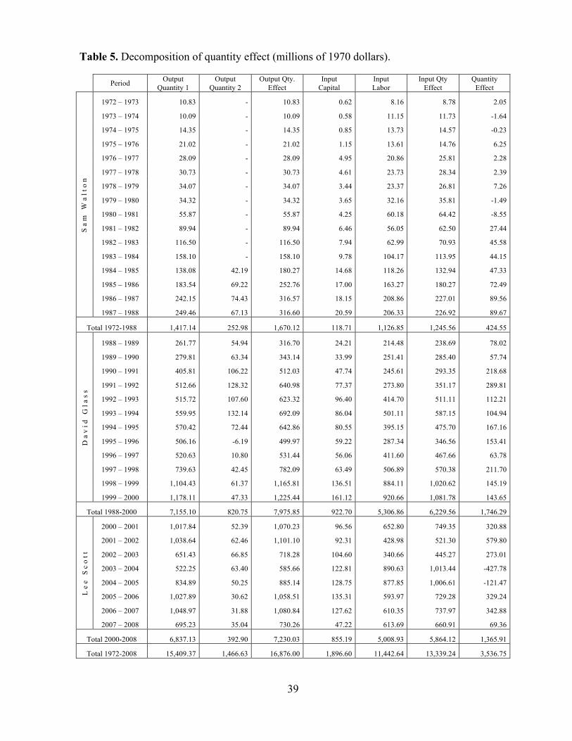
39

Table 5. Decomposition of quantity effect (millions of 1970 dollars).

Period Output Quantity 1

Output Quantity 2

Output Qty. Effect

Input Capital

Input Labor

Input Qty Effect

Quantity Effect

Sa

m W

alt

on

1972 – 1973 10.83 - 10.83 0.62 8.16 8.78 2.05

1973 – 1974 10.09 - 10.09 0.58 11.15 11.73 -1.64

1974 – 1975 14.35 - 14.35 0.85 13.73 14.57 -0.23

1975 – 1976 21.02 - 21.02 1.15 13.61 14.76 6.25

1976 – 1977 28.09 - 28.09 4.95 20.86 25.81 2.28

1977 – 1978 30.73 - 30.73 4.61 23.73 28.34 2.39

1978 – 1979 34.07 - 34.07 3.44 23.37 26.81 7.26

1979 – 1980 34.32 - 34.32 3.65 32.16 35.81 -1.49

1980 – 1981 55.87 - 55.87 4.25 60.18 64.42 -8.55

1981 – 1982 89.94 - 89.94 6.46 56.05 62.50 27.44

1982 – 1983 116.50 - 116.50 7.94 62.99 70.93 45.58

1983 – 1984 158.10 - 158.10 9.78 104.17 113.95 44.15

1984 – 1985 138.08 42.19 180.27 14.68 118.26 132.94 47.33

1985 – 1986 183.54 69.22 252.76 17.00 163.27 180.27 72.49

1986 – 1987 242.15 74.43 316.57 18.15 208.86 227.01 89.56

1987 – 1988 249.46 67.13 316.60 20.59 206.33 226.92 89.67

Total 1972-1988 1,417.14 252.98 1,670.12 118.71 1,126.85 1,245.56 424.55

Da

vid

Gla

ss

1988 – 1989 261.77 54.94 316.70 24.21 214.48 238.69 78.02

1989 – 1990 279.81 63.34 343.14 33.99 251.41 285.40 57.74

1990 – 1991 405.81 106.22 512.03 47.74 245.61 293.35 218.68

1991 – 1992 512.66 128.32 640.98 77.37 273.80 351.17 289.81

1992 – 1993 515.72 107.60 623.32 96.40 414.70 511.11 112.21

1993 – 1994 559.95 132.14 692.09 86.04 501.11 587.15 104.94

1994 – 1995 570.42 72.44 642.86 80.55 395.15 475.70 167.16

1995 – 1996 506.16 -6.19 499.97 59.22 287.34 346.56 153.41

1996 – 1997 520.63 10.80 531.44 56.06 411.60 467.66 63.78

1997 – 1998 739.63 42.45 782.09 63.49 506.89 570.38 211.70

1998 – 1999 1,104.43 61.37 1,165.81 136.51 884.11 1,020.62 145.19

1999 – 2000 1,178.11 47.33 1,225.44 161.12 920.66 1,081.78 143.65

Total 1988-2000 7,155.10 820.75 7,975.85 922.70 5,306.86 6,229.56 1,746.29

Le

e S

co

tt

2000 – 2001 1,017.84 52.39 1,070.23 96.56 652.80 749.35 320.88

2001 – 2002 1,038.64 62.46 1,101.10 92.31 428.98 521.30 579.80

2002 – 2003 651.43 66.85 718.28 104.60 340.66 445.27 273.01

2003 – 2004 522.25 63.40 585.66 122.81 890.63 1,013.44 -427.78

2004 – 2005 834.89 50.25 885.14 128.75 877.85 1,006.61 -121.47

2005 – 2006 1,027.89 30.62 1,058.51 135.31 593.97 729.28 329.24

2006 – 2007 1,048.97 31.88 1,080.84 127.62 610.35 737.97 342.88

2007 – 2008 695.23 35.04 730.26 47.22 613.69 660.91 69.36

Total 2000-2008 6,837.13 392.90 7,230.03 855.19 5,008.93 5,864.12 1,365.91

Total 1972-2008 15,409.37 1,466.63 16,876.00 1,896.60 11,442.64 13,339.24 3,536.75

40

Appendix: A Review of the Literature on Walmart

Books, research articles and even documentaries have been made about Walmart. The

aspects analyzed in these sources vary considerably, as do the standpoints of the authors. This

section does not intend to be an exhaustive literature review on the subject of Walmart; we

merely concentrate on the most relevant works for our research.

One of the most important sources about Walmart’s business model consists of the

books written by insiders like Sam Walton and Don Soderquist (former COO). In his memoirs,

Walton offers his viewpoint on how he built Walmart. Walton dwelt on the history of the

company and gave insight into his decision-making process. Obviously, both Soderquist and

Walton portrayed the company in a good light, and gave advice for future entrepreneurs.

Some of the works available are compilations of research articles written by authors

from distinct fields of study. “Wal-Mart World” by Stanley Brunn (2006) and “Wal-Mart, The

face of twenty-first century capitalism” by Nelson Lichtenstein (2006) are examples of this

literature. Several issues are covered in these books ranging from human resource policies to

zoning.

Other authors attempt to explain Walmart’s success by recognizing particular strategies

employed by the giant of Bentonville. “The Walmart Effect” by Charles Fisher and “Walmart

Triumph” by Robert Slater are examples. Harvard Business School has published several

business case studies on Walmart (Ghemawat, 1989 and 2007; Bradley & Ghemawat, 2002;

Ghemawat, Mark & Bradley, 2004 and Oberholzer-Gee, 2006). In this literature, the authors

provide facts about the company, describe strategies pursued by the firm, and list challenges

and opportunities for future years.

One of the best-known facts about Walmart is its obsession with low prices. “Always

low prices, always” was the company’s slogan for many years. EDLP is defined “as fixing low

prices so the customers could be sure that these prices won’t change erratically by frequent

promotional activities.”28,29 Several studies have been carried out in an attempt to demonstrate

that Walmart does indeed charge low prices. Basker (2005) finds that Walmart’s presence in a

given geography lowers prices between 1.5-3% in the short run and 7-13% in the long run.

Walmart itself appointed the company Global Insight to conduct a study of the economic

41

impact of Walmart’s operations. The results, presented in 2005, showed that Walmart

contributed to lowering the prices of food-at-home (9.1%) and commodities (4.2%) and to the

decline of overall consumer prices (3.1%) between 1985 and 2004. Basker & Noel (2009)

analyze how prices change in a community when Walmart opens a supercenter (discount store

plus groceries). Walmart prices were 10% lower than its competitors, according to the results

of the study. In addition, competing stores reduce their prices by between 1% to 1.2%.

Of course, a reputation for low prices could mean a reputation for low quality products

as well. According to Hausman and Leibtag (2007), the Bureau of Labor Statistics (BLS) in

the United States considers that customers do not receive the same quality service when

shopping at Walmart as in other retail stores. The BLS justifies the price gap by this alleged

difference in service quality. Following this reasoning, Basker (2005b) conducted a study to

determine whether Walmart sells inferior goods in the strictly economic sense. She finds that,

ceteris paribus, a 1% reduction in personal disposable income increases Walmart’s revenue by

0.5%.30 This researcher offers two explanations for these results. On the one hand, it could be

that the majority of households view shopping at Walmart as an inferior activity. On the other

hand, it may be that the subset of households that hold this view has greater elasticity of

demand.

Another topic discussed is the relationship between Walmart and its employees. We

have to make a distinction between supervisory/managerial ranks and non-managerial

workers. Bradley & Ghemawat (2002) explain that store managers remuneration is based on

store sales and profits. In the case of non-managerial workers, besides their salaries, they

benefit from a profit-sharing plan to which managers also have access.

One of the issues usually analyzed is whether Walmart creates jobs or destroys them.

Two studies, Basker (2005b) and Global Insight (2005), find that Walmart presence increased

the number of jobs available in the communities where the company placed its stores.

However, several authors have raised the concerns about the quality of these new jobs.

Greenhouse (2003) reported that the average pay of a sales clerk at Walmart in 2003

was $8.50 per hour, or about $14,000 a year. This amount was $1,000 below the poverty line

for a family of three. Furthermore, in a 2005 presentation given by Arindrajit Dube and Steve

Wertheim (University of California at Berkeley, Labor Center), it was reported that Walmart’s

42

workers’ wages were 12.4% lower than those earned by other workers in the retail industry

and 14.5% less than the wages paid to employees working in large retail in general.

The secrecy of Walmart’s labor costs was partially broken as a by-product of

proceedings in a court case. In June 2001, six workers filed a lawsuit against Walmart, in what

has become the largest class-action lawsuit in United States. As part of the collection of

evidence for the case, Professor Richard Drogin was appointed to answer questions raised by

the plaintiffs. Walmart submitted valuable information about workers’ remuneration. In

February 2003, Drogin presented his conclusions.

Drogin (2003) found that although women made up more than two-thirds of the total

workforce from 1996 to 2001, they were disproportionately employed in low-earning

positions. Furthermore, women working in similar positions to men earned 5% to 15% less

than men, after controlling for factors like such as seniority, status, and store. Drogin stated

that the disparity increases if performance is included in the study. The company defended

itself against this accusation by claiming that women were less likely to apply for managerial

positions because these positions required constant moving between cities (as reported in

Oberholzer-Gee, 2006). Nevertheless, a highly feminized workforce was coherent with what

was explained by Fishman (2006). The author suggests that the management conceived the

Walmart workforce as mainly housewives trying to earn a supplementary income for their

families. From this perspective, workers clearly needed their spouses' income and the

healthcare benefits to survive. Dube and Jacobs (2004) made the claim that when workers

cannot cover their basic needs with their spouses’ income and healthcare benefits, they have to

rely on public assistance. These authors tried to measure the Walmart effect on the public

accounts of the state of California.31 Hausman and Leibtag (2007) suggest that, when

measuring the welfare effects of Walmart, however, its influence on prices should be included

in order to gain a complete understanding. They state that the company’s low prices more than

compensate for its low wages, making the net effect positive.

Besides prices and wages, some papers analyze the expansion patterns followed by

Walmart. The idea behind these studies is that Walmart’s expansion patterns helped the

company reduce costs and compete effectively against its rivals. However, Walmart's presence

in some communities implied problems such as urban sprawl.

43

Basker (2005) estimates that each new Walmart store accounts for the failure of 4

small stores and 0.7 medium size stores after 5 years of entry. Although this appears to be a

general trend in the retail sector between 1977 to 2002, the number of “mom-and-pop” stores

fell by nearly 40%, and the number of small chains by 75% (Basker et al., 2008). A study

carried out by Jia (2008) reported that Walmart’s expansion accounts for approximately 40-

50% of the variation in the net number of small stores and 30-40% for all other discount

stores.

According to Graff and Ashton (1994), Walmart followed neighborhood expansion

diffusion and reverse hierarchical diffusion. This means that the company expanded to

locations that were a short distance from its current facilities. The main advantage of this

expansion policy is the development of a dense distribution network. Graff (1998) claims that

this density allowed Walmart to spread the advertisement costs and reduce distribution costs.

This idea is explored by Holmes (2008). Both authors, Holmes and Graff, affirm that the

introduction of the “supercenter format” in the late 1980s followed the same path of expansion

as the initial discount stores. Holmes (2008) claims that “Walmart never jumped to some far

off location to later fill in the area in the inside out” (p. 1). The downside of the “economies of

density” in the retail industry is the cannibalization of the sales by the older stores. Walmart

estimates that this effect represents 1% of the sales of the stores in 2006 and 1.5% in 2007 and

2008.32,33

The internationalization of Walmart is a new topic that has been explored recently.

According to Burt and Spark (2006), three phases can be distinguished in the international

expansion of the firm. Firstly, the company opened stores in adjacent markets such as Mexico

and Canada. Then it started the “flag-planting phase,” during which the firm started new

businesses in a wide range of countries. Some of the new ventures were successful, as in the

case of China, and others did not go well (e.g. Indonesia, Hong Kong, and South Korea).

There was also stagnation in Germany, Argentina, and Brazil due to regulatory pressure or

other barriers. Finally, in the third phase, the company decided to invest carefully, purchasing

already successful chains like ASDA in the United Kingdom and Seiyu in Japan.

Another benefit of internationalization is its impact on the supply chain. China has

played a major role in Walmart’s expansion as a supplier of cheap goods for sale. Basker and

44

Pham Hoang (2008) explore this issue and emphasize that Walmart’s imports from China

accounted for 15% of total US imports of goods from that country. These authors conclude

that the combination of low trade barriers and high investment in technology are the main

causes of Walmart’s growth. According to their calculations, 60% of Walmart’s growth is

explained by technological innovation and the other 40% is explained by the reduction of

input costs due primarily to tariff reductions and changes in sourcing.

The one-stop-shopping effect is an additional element that has been analyzed in the

literature about Walmart. Basker, Klimek and Hoang Van (2008) demonstrate that there is a

complementary relationship between the economies of scale and scope that benefit Walmart

and other big box retailers. The hypothesis is that as the companies increase the number of

stores, they gain economies of scale. In addition, these companies offer a broader assortment

of products generating economies of scope. The larger diversity of products attracts customers

who want to avoid the transport costs inherent in buying at several stores. This situation is

known as the “one-stop-shopping effect” or economies of scale on the demand side due to

savings in transport costs (Basker et al., 2008). These authors find that, for every store opened,

a retail company adds an additional product line to an existing store. Furthermore, when the

company incorporates a new line in its current stores, this action entails the opening of 400

new stores competing in more than 8,000 new markets.

Endnotes

1 The recent Long Range Planning special issue on business models (April 2010) received more than 80 submissions and attracted contributions from scholars such as David Teece and Nobel prize winning practitioner Muhammad Yunus. Zott, Amit and Massa (2010) review the growing literature in management on business models. 2 Drucker, Peter, The Practice of Management, Harper and Row Publishers, 1954. A Google search for “Business Model” in October 2012 yielded 31.1 million hits. 3 See Long Range Planning call for papers for the Special Issue on “Business Models” by Charles Baden-Fuller, Ian MacMillan, Benoît Demil, and Xavier Lecocq. 4 The theory of index numbers studies different ways in which information may be aggregated. Government statistics departments use index numbers to better understand economic performance and its evolution. The roots of this theory can be traced back to the 19th century. Fisher (1911) made important early developments and Balk (2008) provides an updated revision of the theory.

45

5 Davis (1955) was a pioneer in proposing this scheme, which was followed by Kendrick and Creamer (1961) and Kendrick (1984). Other researchers such as Genescà and Grifell-Tatjé (1992), Kurosawa (1975, 1991), Miller (1984); and Miller and Rao (1989) present further developments. 6 Bennet (1920) advocates using the arithmetic mean of price and quantities to evaluate change. We follow this approach because Diewert (2005) has shown that the Bennet indicators have a set of properties that make them superior to the traditional Laspeyres and Paasche indicators. 7 Choices are represented using bold and underlined fonts; rigid consequences are in boxes and flexible consequences are shown in plain text. The arrows connecting choices and consequences are those provided by theories explaining causal relationships. 8 Casadesus-Masanell and Ricart (2008), p. 9. 9 For this section of the paper we consulted several research articles: Barbaro and Gills (2005), Basker and Pham Hoang (2008), Basker, (2005a,b), Basker and Noel (2007), Basker, Klimek, and Pham Hoang (2008) Bonacich and Wilson (2006), Bradley and Ghemawat (2002), Burt and Sparks (2006), Drogin (2003), Dube and Jacobs (2004), Dube and Wertheim (2005), Dunnett and Arnold (2006), Fishman (2006), Ghemawat (1989), Ghemawat, Mark and Bradley (2004), Global Insight Inc., (2005), Graff (1998), Graff and Ashton (1994), Hausman and Leibtag (2007), Holmes (2008), Jia (2008) and Oberholzer-Gee (2006). In the appendix, we discuss the literature on Walmart reviewed for this paper. 10 Walton (1992, p. 80). 11 Walton (1992, p. 109). 12 Walmart Annual Report (1975, p. 2). 13 Elements of “Aggressive Hospitality” had been applied earlier on a non-formal basis. 14 Walmart also offered premium brands such as “Sam’s American Choice,” which were manufactured in the U.S. 15 This was an important change in Walmart’s merchandising mix. Food items have lower markups than products traditionally sold by discount retailers. 16 The U.S. Supreme Court rejected the class-action lawsuit in June 20, 2011. The Court denied that the lawsuit fulfilled the requirements of a “class-action rules.” See Liptak, Adam (2011). 17 Some of these business ventures failed (e.g. Germany and Korea) which might have encouraged Walmart to change course towards a more painstaking international expansion as related by Burt and Spark (2006). 18 Although we use production theory, we bypass the very restrictive assumptions embedded in neoclassical microeconomics and, thus, the methodology that we present is applicable to a broad set of institutional contexts. Cyert and Hedrick (1972) characterize this issue correctly when they state: “The unmodified neoclassical approach is characterized by an ideal market with firms for which profit maximization is the single determinant of behavior” (p. 400) and also “Many papers are based on…modifications of the neoclassical method. They extend the model to deal with real-world issues not faced by the simple text-book models, but retain the a priori character, in that all of the detail added is descriptive of the environment,” (p. 401). 19 See http://walmartstores.com/aboutus/297.aspx 20 In the case of Costco, the company merged with Price in the year 1993. We therefore treat Costco as two separate firms, one prior to the merger and other after the merger. Kmart filed for bankruptcy in 2002. The successor company survived for two years before merging with Sears. Each circumstance was treated as a separate case (three firms). May Department Stores was treated as two separate companies, one before the acquisition of Caldor and the other after the acquisition. We include information about May only until 2003. Kmart, Target and May had multiple retail formats during the period of study. The financial information on these businesses is not separated from the discount retailing activities. We do not consider this a problem, as all these activities are in the same line of business. The same is not true for Sears which had a very broad spectrum of businesses besides retailing (e.g. Dean Witter, Allstate Insurance Company, Coldwell Banker among others). For this reason, it was essential to analyze the merchandise part only. Fortunately, Sears discloses information on each division separately. We therefore include only the retail part of Sears.

46

21 We do not have information about the value added amount for each type of retail format, discount and warehouse club at Walmart. However, we know the total sales and the operating profit obtained by each branch for every year in the sample. We assume that the value added is distributed in the same way as the income variable is distributed each year. 22 Our computations were programmed in the statistical package R. For calculating the input distance functions, we used the package FEAR (Frontier Efficiency Analysis for R) made by Paul Wilson. 23 The only exception was the period 1973-1974 (see Table 4). The explanation for this fall in profits was the adoption of the LIFO method of costing inventory. The accounting change resulted in a reduction in earnings of 1.8 million 1970 dollars in real terms, although the company profits grew if measured in current dollars. 24Output prices are measured as value added per dollar of sales. 25 When Walton left the CEO position in 1988, there were 105 Sam’s Club stores; by 1991 that number was 205. See the development of the output quantity effect for Sam’s Club in Table 5. 26 See Walmart Annual Report 1998, page 5; Walmart Annual Report 27 Walmart applied a new pay structure for U.S. workers in 2004. 28 Wal-Mart. “Annual Report 2006.” 2006., p21. 29 Nevertheless, sometimes the company carries out promotional activities, such as Rollback prices. This activity consists of cutting prices even further for prolonged periods of time, sometimes indefinitely. 30 This is an upper boundary. The author claims that a more realistic figure is 0.7%. 31 Dube and Jacobs (2004) used Drogin’s data plus other sources to calculate the effect of Walmart’s presence on the public accounts of California. The researchers concluded that Walmart finances its operations with public money. Walmart’s annual cost to California tax-payers was $86 million dollars, distributed into $32 million for health-related benefits and $54 million in other assistance during the year the study was conducted. They estimate that Walmart’s employees use 40% more public healthcare money than the average families of all retail employees. The author claims that Walmart’s effect on public finances may have been underestimated. For instance, not all the people who are eligible for public assistance apply for it. Dube and Jacobs (2004) comment, that in a program broadcasted by PBS, it was reported that Walmart gave their employees a 1-800 number to determine their eligibility. So, if Walmart instructs its employees on how to obtain public assistance, the total effect would be greater than that reported in the study. 32 Wal-Mart. “Annual Report 2006.” 2006, p22. 33 Wal-Mart. “Annual Report 2008.” 2008, p13.