Embed Size (px)
Citation preview
Business Statistics 41000:
Simple Linear Regression
Drew D. Creal
University of Chicago, Booth School of Business
March 7 and 8, 2014
1

Class information
I Drew D. Creal
I Email: [email protected]
I Office: 404 Harper Center
I Office hours: email me for an appointment
I Office phone: 773.834.5249
http://faculty.chicagobooth.edu/drew.creal/teaching/index.html
2
Course schedule
I Week # 1: Plotting and summarizing univariate data
I Week # 2: Plotting and summarizing bivariate data
I Week # 3: Probability 1
I Week # 4: Probability 2
I Week # 5: Probability 3
I Week # 6: In-class exam and Probability 4
I Week # 7: Statistical inference 1
I Week # 8: Statistical inference 2
I Week # 9: Simple linear regression
I Week # 10: Multiple linear regression
3
Outline of today’s topics
I. Motivation: why regression?
II. The simple linear regression model
III. Interpretation of the regression parameters
IV. Regression as a model of P(Y = y |X = x)
V. Estimation of the regression parameters
VI. Plug-in prediction
V. Confidence Intervals and Hypothesis Tests for theRegression Parameters
VIII. Fits, residuals, and R-squared
IX. Application: The Market Model
4
Motivation: why regression?
5
Motivation: why regression?
Regression is a useful tool for many reasons.
The most important are:
I Prediction/forecasting
I Measuring dependence (e.g. correlation) betweenvariables.
6
Motivation: why regression?
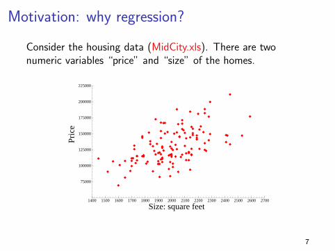
Consider the housing data (MidCity.xls). There are twonumeric variables “price” and “size” of the homes.
1400 1500 1600 1700 1800 1900 2000 2100 2200 2300 2400 2500 2600 2700
75000
100000
125000
150000
175000
200000
225000
Size: square feet
Pric
e
7
Motivation: why regression?
I Consider only the data on housing prices.
I For the moment, assume we do not observe house sizes.
I After Lectures # 3-7, we recognize that our sample ofn = 128 homes is exactly that....a sample.
I What if we are interested in learning about the populationand want to account for sampling uncertainty?
I After all, we could have observed a different sample ofhouses.
I How could we model the price of a house usingprobability?
8

Motivation: why regression?
We can define a r.v. Yi to be the price of the i -th house!
It is a r.v. because before the house is sold we do not knowhow much it will sell for.
We treat our data (y1, y2, . . . , yn) as the outcome of asequence of r.v.’s (Y1,Y2, . . . ,Yn).
We can model this data with an i.i.d. Normal model.
p(y1, y2, . . . , yn) = p(y1) ∗ p(y2) ∗ · · · ∗ p(yn)
In other words, each observation is a normal r.v.
p(yi) = N(µ, σ2)
9
Motivation: why regression?
Suppose you are going to sell your house in this city.
You are interested in the average price µ of a house.
I Following Lectures #7-8, we can perform statisticalinference for the parameters of interest, e.g. E[Y ] = µ.
I For example, we could use x as an estimator of µ.
I We can use x to predict what the house Yi will sell for.
But, we are ignoring information about house sizes!!
We are currently only looking at the marginal distribution P(Y = y).
10
Motivation: why regression?
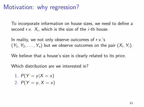
To incorporate information on house sizes, we need to define asecond r.v. Xi , which is the size of the i -th house.
In reality, we not only observe outcomes of r.v.’s(Y1,Y2, . . . ,Yn) but we observe outcomes on the pair (Xi ,Yi).
We believe that a house’s size is clearly related to its price.
Which distribution are we interested in?
1. P(Y = y |X = x)
2. P(Y = y ,X = x)
11

Motivation: why regression?
Which distribution are we interested in?
1. P(Y = y |X = x)
2. P(Y = y ,X = x)
Since we believe that a house’s size is clearly related to itsprice, we think that P(Y = y |X = x) 6= P(Y = y).
KEY POINT: Regression provides a simple way to model theconditional distribution of Y given X = x .
This allows us to incorporate our information on house sizes.
It may help us improve our prediction of house prices.
12
Simple Linear Regression
(NOTE: The term “simple” linear regression means we are looking at a relationship
between two variables. In Lecture # 10, we will do multiple linear regression (one y ,
lots of x ’s). )
13

Simple Linear Regression
When doing regression, we care about the conditionaldistribution P(Y = y |X = x) = p(y |x).
We use the following terminology:
I Y is the dependent variable.
I X is the independent variable, the explanatory variable, orsometimes just the regressor.
14
Simple Linear Regression
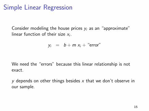
Consider modeling the house prices yi as an “approximate”linear function of their size xi .
yi = b + m xi + “error”
We need the “errors” because this linear relationship is notexact.
y depends on other things besides x that we don’t observe inour sample.
15
Simple Linear Regression
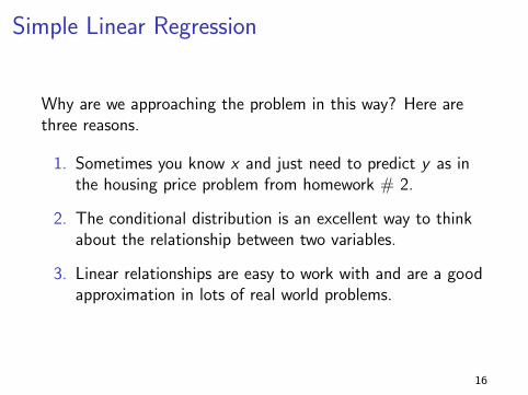
Why are we approaching the problem in this way? Here arethree reasons.
1. Sometimes you know x and just need to predict y as inthe housing price problem from homework # 2.
2. The conditional distribution is an excellent way to thinkabout the relationship between two variables.
3. Linear relationships are easy to work with and are a goodapproximation in lots of real world problems.
16
Simple Linear Regression
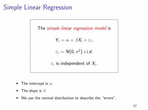
The simple linear regression model is
Yi = α + βXi + εi .
εi ∼ N(0, σ2) i.i.d.
εi is independent of Xi .
I The intercept is α.
I The slope is β.
I We use the normal distribution to describe the “errors”.
17
Simple Linear Regression: Remarks
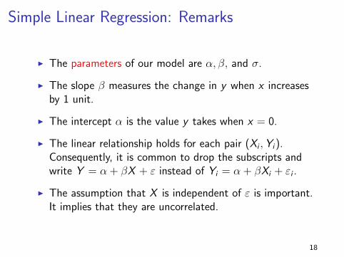
I The parameters of our model are α, β, and σ.
I The slope β measures the change in y when x increasesby 1 unit.
I The intercept α is the value y takes when x = 0.
I The linear relationship holds for each pair (Xi ,Yi).Consequently, it is common to drop the subscripts andwrite Y = α + βX + ε instead of Yi = α + βXi + εi .
I The assumption that X is independent of ε is important.It implies that they are uncorrelated.
18
Simple Linear Regression: Remarks
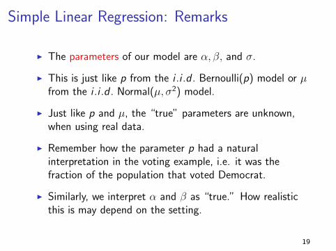
I The parameters of our model are α, β, and σ.
I This is just like p from the i .i .d . Bernoulli(p) model or µfrom the i .i .d . Normal(µ, σ2) model.
I Just like p and µ, the “true” parameters are unknown,when using real data.
I Remember how the parameter p had a naturalinterpretation in the voting example, i.e. it was thefraction of the population that voted Democrat.
I Similarly, we interpret α and β as “true.” How realisticthis is may depend on the setting.
19
Interpretation of the regression
parameters α, β, and σ
20
IMPORTANT
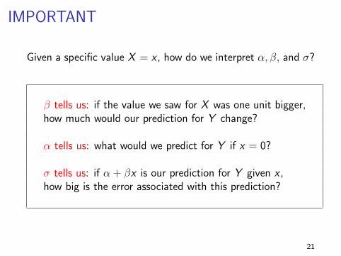
Given a specific value X = x , how do we interpret α, β, and σ?
β tells us: if the value we saw for X was one unit bigger,how much would our prediction for Y change?
α tells us: what would we predict for Y if x = 0?
σ tells us: if α + βx is our prediction for Y given x ,how big is the error associated with this prediction?
21
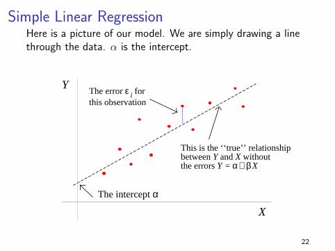
Simple Linear RegressionHere is a picture of our model. We are simply drawing a linethrough the data. α is the intercept.
X
YThe error ε i for this observation
This is the ‘‘true’’ relationship between Y and X without the errors Y = α+ β X
The intercept α
22
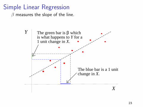
Simple Linear Regressionβ measures the slope of the line.
X
Y
The blue bar is a 1 unit change in X.
The green bar is β whichis what happens to Y for a1 unit change in X.
23
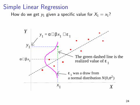
Simple Linear RegressionHow do we get y1 given a specific value for X1 = x1?
X
Y
x1
y1
y1 = α+ β x1 + ε 1
The green dashed line is therealized value of ε 1
α+ β x1
ε 1 was a draw froma normal distribution N(0,σ2)
24
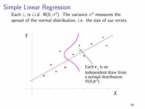
Simple Linear RegressionEach εi is i.i.d. N(0, σ2). The variance σ2 measures thespread of the normal distribution, i.e. the size of our errors.
X
Y
Each ε i is an independent draw from a normal distribution N(0,σ2)
25
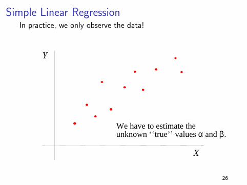
Simple Linear RegressionIn practice, we only observe the data!
X
Y
We have to estimate the unknown ‘‘true’’ values α and β.
26
Simple Linear Regression
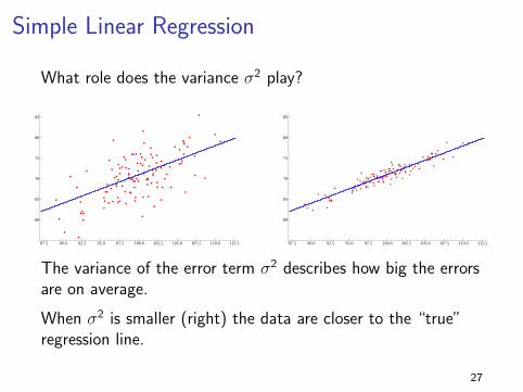
What role does the variance σ2 play?
87.5 90.0 92.5 95.0 97.5 100.0 102.5 105.0 107.5 110.0 112.5
60
65
70
75
80
85
87.5 90.0 92.5 95.0 97.5 100.0 102.5 105.0 107.5 110.0 112.5
60
65
70
75
80
85
The variance of the error term σ2 describes how big the errorsare on average.
When σ2 is smaller (right) the data are closer to the “true”regression line.
27
Simple Linear Regression
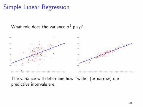
What role does the variance σ2 play?
87.5 90.0 92.5 95.0 97.5 100.0 102.5 105.0 107.5 110.0 112.5
60
65
70
75
80
85
87.5 90.0 92.5 95.0 97.5 100.0 102.5 105.0 107.5 110.0 112.5
60
65
70
75
80
85
The variance will determine how “wide” (or narrow) ourpredictive intervals are.
28
Regression as a model of P(Y = y |X = x)
29
Simple Linear Regression
Regression looks at the conditional distribution of Y given X .
Instead of coming up with a story for the joint distributionp(x , y):
What do I think the next (x , y) pair will be?
Regression just talks about the conditional distribution p(y |x):
Given a value for x , what will the next y be?
30

Regression as a model of P(Y = y |X = x)
Our model is:
Y = α + βX + ε ε ∼ N(0, σ2)
where ε is independent of X .
Regression is a model for the conditional distributionP(Y = y |X = x).
What are the mean and variance of the conditionaldistribution?
I E[Y |X = x ]
I V[Y |X = x ]
31
Regression as a model of P(Y = y |X = x)
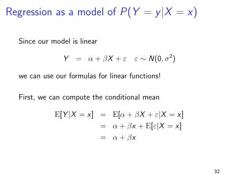
Since our model is linear
Y = α + βX + ε ε ∼ N(0, σ2)
we can use our formulas for linear functions!
First, we can compute the conditional mean
E[Y |X = x ] = E[α + βX + ε|X = x ]
= α + βx + E[ε|X = x ]
= α + βx
32
Regression as a model of P(Y = y |X = x)
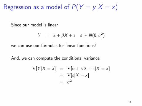
Since our model is linear
Y = α + βX + ε ε ∼ N(0, σ2)
we can use our formulas for linear functions!
And, we can compute the conditional variance
V[Y |X = x ] = V[α + βX + ε|X = x ]
= V[ε|X = x ]
= σ2
33
Regression as a model of P(Y = y |X = x)
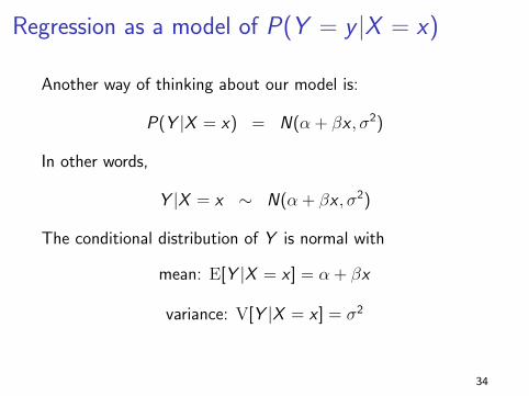
Another way of thinking about our model is:
P(Y |X = x) = N(α + βx , σ2)
In other words,
Y |X = x ∼ N(α + βx , σ2)
The conditional distribution of Y is normal with
mean: E[Y |X = x ] = α + βx
variance: V[Y |X = x ] = σ2
34
Prediction using P(Y = y |X = x)
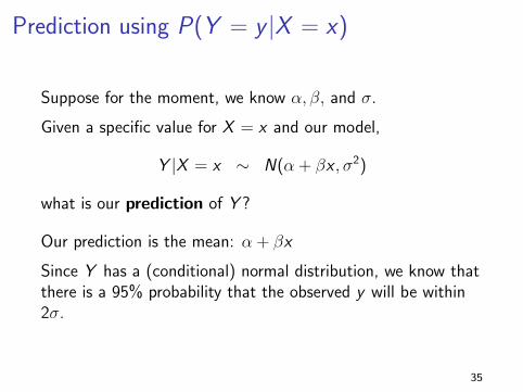
Suppose for the moment, we know α, β, and σ.
Given a specific value for X = x and our model,
Y |X = x ∼ N(α + βx , σ2)
what is our prediction of Y ?
Our prediction is the mean: α + βx
Since Y has a (conditional) normal distribution, we know thatthere is a 95% probability that the observed y will be within2σ.
35
Prediction using P(Y = y |X = x)
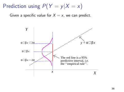
Given a specific value for X = x , we can predict.
X
Y
x
α+ β x
y = α+ β xα+ β x + 2σ
α+ β x − 2σThe red line is a 95% predictive interval, i.e. the ‘‘empirical rule’’.
36
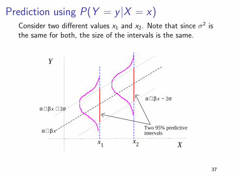
Prediction using P(Y = y |X = x)Consider two different values x1 and x2. Note that since σ2 isthe same for both, the size of the intervals is the same.
X
Y
x1
α+ β x
α+ β x + 2σ
α+ β x − 2σ
x2
Two 95% predictive intervals
37

Prediction using P(Y = y |X = x)
Important.
1. The width of the prediction interval produced fromP(Y = y |X = x) will (typically) be smaller thanP(Y = y).
2. The variance of the conditional distributionP(Y = y |X = x) cannot be larger than the variance ofP(Y = y).
3. Using information on X will help us predict Y .
4. We can see this visually on the house price data (nextslide).
38
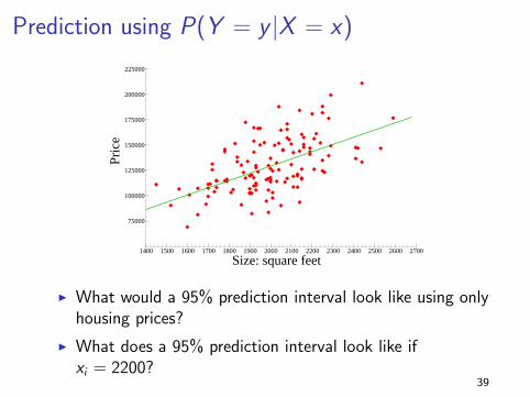
Prediction using P(Y = y |X = x)
1400 1500 1600 1700 1800 1900 2000 2100 2200 2300 2400 2500 2600 2700
75000
100000
125000
150000
175000
200000
225000
Size: square feet
Pric
e
I What would a 95% prediction interval look like using onlyhousing prices?
I What does a 95% prediction interval look like ifxi = 2200?
39
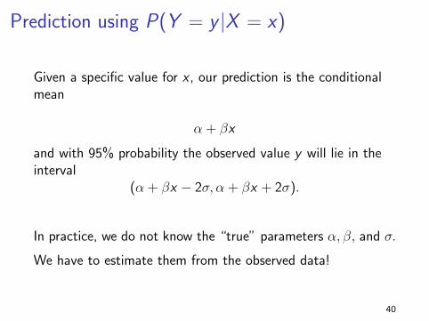
Prediction using P(Y = y |X = x)
Given a specific value for x , our prediction is the conditionalmean
α + βx
and with 95% probability the observed value y will lie in theinterval
(α + βx − 2σ, α + βx + 2σ).
In practice, we do not know the “true” parameters α, β, and σ.
We have to estimate them from the observed data!
40
Estimation of the regression
parameters α, β, and σ
41
Estimates
In Lectures #7 and #8, we investigated two models:
I i .i .d . Bernoulli(p) model with unknown parameter p.
I i .i .d . Normal(µ, σ2) model with unknown parameter µ.
We chose estimators and considered the sampling distributionsof the estimators.
I For the i .i .d . Bernoulli(p) model, we used p as anestimator of the unknown parameter p.
I For the i .i .d . Normal(µ, σ2) model, we used x as anestimator of the unknown parameter µ.
The goal in this section is to find estimators for α, β, and σ.
42
Estimates
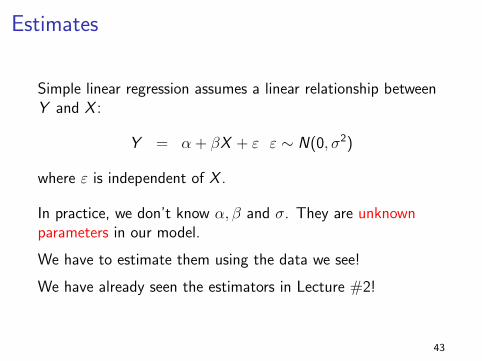
Simple linear regression assumes a linear relationship betweenY and X :
Y = α + βX + ε ε ∼ N(0, σ2)
where ε is independent of X .
In practice, we don’t know α, β and σ. They are unknownparameters in our model.
We have to estimate them using the data we see!
We have already seen the estimators in Lecture #2!
43
Linear regression formulas
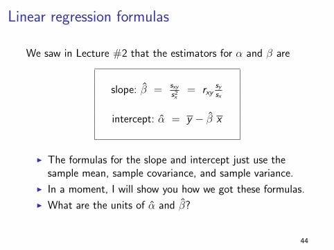
We saw in Lecture #2 that the estimators for α and β are
slope: β = sxys2x
= rxysysx
intercept: α = y − β x
I The formulas for the slope and intercept just use thesample mean, sample covariance, and sample variance.
I In a moment, I will show you how we got these formulas.
I What are the units of α and β?
44
Estimates
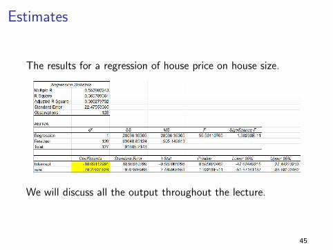
The results for a regression of house price on house size.
We will discuss all the output throughout the lecture.
45
How do we interpret the estimates?
You can (and should!) interpret β as saying “a house that is1000 square feet larger sells for about $70,000 more”.
You probably should not interpret α as saying “the price of ahouse of size zero is -$10,000”. Are there any houses of sizezero in our data?
Would we want to use this data to predict the price of an8,000 square foot mansion?
46

Estimates
Given our estimates of α and β, these determine a newregression line
y = α + βx
which is called the fitted regression line.
Remember that due to sampling error, our estimate α is notgoing to be exactly equal to α and our estimate β is not goingto be exactly equal to β.
Consequently, the fitted regression line is not going to beexactly equal to the “true” regression line:
y = α + βx
47
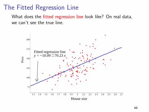
The Fitted Regression LineWhat does the fitted regression line look like? On real data,we can’t see the true line.
1.3 1.4 1.5 1.6 1.7 1.8 1.9 2 2.1 2.2 2.3 2.4 2.5 2.6 2.7
75
100
125
150
175
200
Pric
e
House size
Fitted regression line y = −10.09 + 70.23 x
48
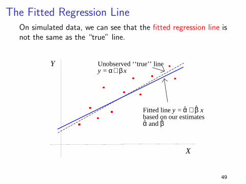
The Fitted Regression LineOn simulated data, we can see that the fitted regression line isnot the same as the “true” line.
X
Y
Fitted line y = α + β x based on our estimates α and β
Unobserved ‘‘true’’ liney = α+ β x
49
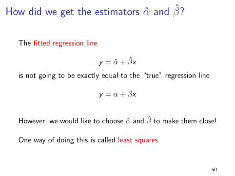
How did we get the estimators α and β?
The fitted regression line
y = α + βx
is not going to be exactly equal to the “true” regression line
y = α + βx
However, we would like to choose α and β to make them close!
One way of doing this is called least squares.
50

Linear regression formulas
Define the residual as ei = yi − (α + βxi). The residual is thedistance between the observed yi and the corresponding pointon our fitted line α + βxi .
(NOTE: We will discuss these concepts in more detail further below.)
α and β are the least squares estimates of α and β.
Using calculus we can show that the estimates α and βminimize the function
SSR =n∑
i=1
(yi − α− βxi
)2where SSR stands for the sum of squared residuals.
51

Estimates
What do the residuals look like?
1.3 1.4 1.5 1.6 1.7 1.8 1.9 2 2.1 2.2 2.3 2.4 2.5 2.6 2.7
75
100
125
150
175
200
Pric
e
House size
Fitted regression line y = −10.09 + 70.23 x
Three different residualsei = yi + 10.09 − 70.23 xi
52

Linear regression formulas
Our estimate of σ is just the sample standard deviation of theresiduals ei .
se =
√∑ni=1 e2in−2 =
√∑ni=1(yi−α−βxi)
2
n−2
I Here we divide by n − 2 instead of n − 1 for the sametechnical reasons (to get an unbiased estimator).
I se just asks, “on average, how far are our observed valuesyi away from the line we fitted?”
53
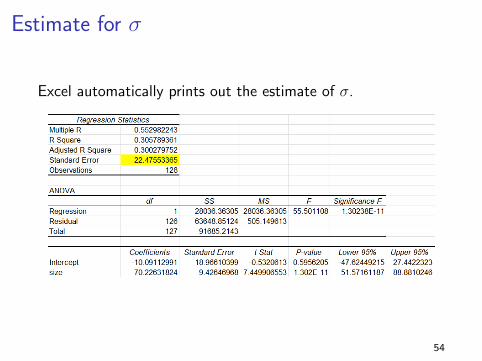
Estimate for σ
Excel automatically prints out the estimate of σ.
54
Plug-in prediction
55
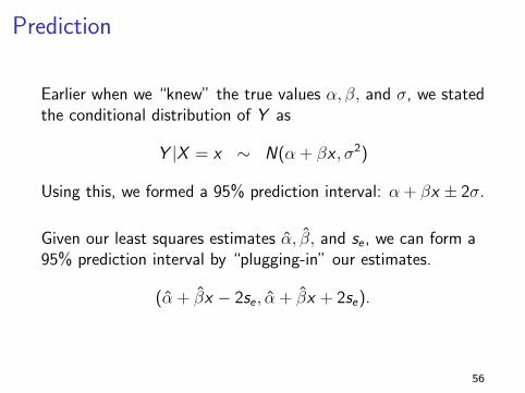
Prediction
Earlier when we “knew” the true values α, β, and σ, we statedthe conditional distribution of Y as
Y |X = x ∼ N(α + βx , σ2)
Using this, we formed a 95% prediction interval: α + βx ± 2σ.
Given our least squares estimates α, β, and se , we can form a95% prediction interval by “plugging-in” our estimates.
(α + βx − 2se , α + βx + 2se).
56
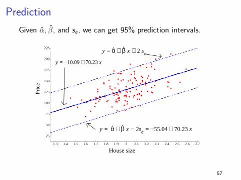
Prediction
Given α, β, and se , we can get 95% prediction intervals.
1.3 1.4 1.5 1.6 1.7 1.8 1.9 2 2.1 2.2 2.3 2.4 2.5 2.6 2.7
25
50
75
100
125
150
175
200
225
Pric
e
House size
y = −10.09 + 70.23 x
y = α + β x − 2se = −55.04 + 70.23 x
y = α + β x + 2 se
57
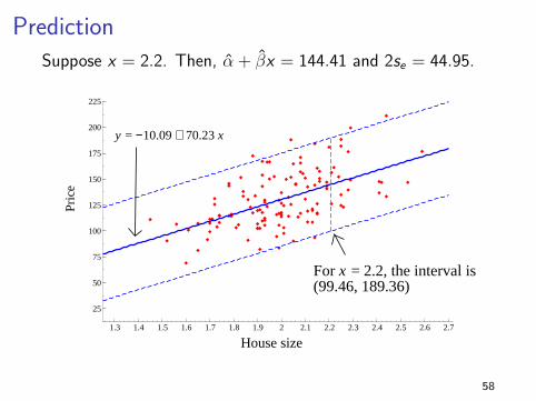
PredictionSuppose x = 2.2. Then, α + βx = 144.41 and 2se = 44.95.
1.3 1.4 1.5 1.6 1.7 1.8 1.9 2 2.1 2.2 2.3 2.4 2.5 2.6 2.7
25
50
75
100
125
150
175
200
225
Pric
e
House size
y = −10.09 + 70.23 x
For x = 2.2, the interval is(99.46, 189.36)
58

Summary: estimators and prediction
Unknown parameter estimatorα α
β βσ se
Given a value for x , the 95% plug-in predictive interval is
α + βx ± 2se
59
Confidence Intervals and Hypothesis
Tests for α, β, and σ
60
Sampling distributions for α and β
Thus far, we have assumed that there exists a “true” linearrelationship
Y = α + βX + ε ε ∼ N(0, σ2)
for unknown parameters α, β, and σ.
I have shown you the formulas for our estimators α, β, and se .
Remember that our estimators are random variables. Why??
61
Sampling distributions for α and β
Recall that we view our estimators α, β and se as randomvariables.
For each possible sample of data that you might observe, youwill likely have different values for α, β, and se .
Sampling error!
For example, there may be many possible samples on houseprices and sizes that you could take resulting in differentvalues for α, β, and se .
62

The Sampling Distribution of an Estimator
The sampling distribution of an estimator is aprobability distribution that describes allthe possible values we might see if we could“repeat” our sample over and over again; i.e., if wecould see other potential samples from thepopulation we are studying.
63
Sampling distributions for α and β
When we view α, β, and se as estimators, they are randomvariables and each will have their own sampling distribution.
It can be shown that (when n is large) the samplingdistributions for α and β are both normal distributions (due tothe CLT).
I won’t derive the mathematical details of the samplingdistributions here like I did for p and x in Lecture #7.
Nevertheless, we can construct standard errors and buildconfidence intervals for the “true” unknown parameters α, β,and σ just like we did for p and µ in Lectures #7 and #8.
64
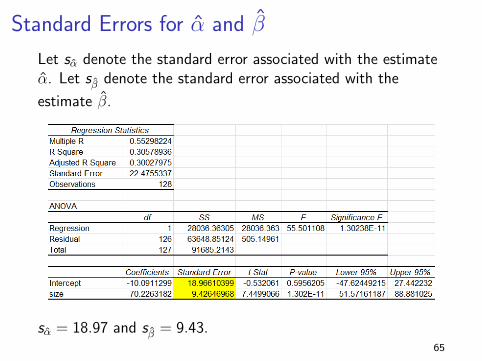
Standard Errors for α and β
Let sα denote the standard error associated with the estimateα. Let sβ denote the standard error associated with the
estimate β.
sα = 18.97 and sβ = 9.43.65
ASIDE: Unbiasedness
As a side note, it can also be shown that α and β are unbiased:
E[α|X ] = α
E[β|X ] = β
Intuitively, our estimate can turn out to be too big or toosmall, but it is not “systematically” too high or too low. Wewill recover the true value on average.
(NOTE: The expectation (or average) is being taken over hypothetical random
samples we might observe from the model.)
66
Confidence Intervals for α and β
We can also build confidence intervals for α and β.
In practice, you will often see confidence intervals for α and βconstructed using the Student’s t distribution instead of thestandard normal.
The reasoning behind this is the same as when we“standardized” the estimator x in Lecture #8.
Again, we are “standardizing” the estimators α and β tocompute the test statistic. This means we are dividing themby the standard errors sα and sβ, which need to be estimatedfrom the data.
67
Confidence Intervals
The 95% confidence interval for α is
α± tval ∗ sα
where tval = T.INV(0.05, n − 2) (NOTE: in Excel)
The 95% confidence interval for β is
β ± tval ∗ sβ
where tval = T.INV(0.05, n − 2) (NOTE: in Excel)
Remember that if n > 30, the tval is roughly 2.68
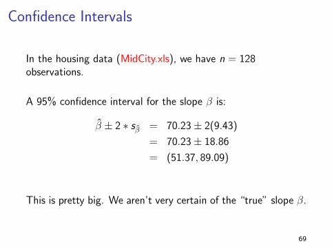
Confidence Intervals
In the housing data (MidCity.xls), we have n = 128observations.
A 95% confidence interval for the slope β is:
β ± 2 ∗ sβ = 70.23± 2(9.43)
= 70.23± 18.86
= (51.37, 89.09)
This is pretty big. We aren’t very certain of the “true” slope β.
69
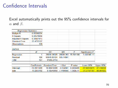
Confidence Intervals
Excel automatically prints out the 95% confidence intervals forα and β.
70
ASIDE: Normality Assumption of ε
Normality of the errors ε in the linear equationY = α + βX + ε is not a crucial assumption.
When the sample size n is large, the sampling distributions ofthe estimators α and β will still be (approximately) normaldistributions.
This is because α and β are just averages of y and x and wecan apply the Central Limit Theorem.
Even if ε is not normal, the confidence intervals will be
95% C.I. for α : α± 2 ∗ sα
95% C.I. for β : β ± 2 ∗ sβ
71
Hypothesis Tests for α and β
Using the sampling distributions of the estimators α and β, wecan also perform hypothesis tests.
Let H0 : α = α0 or H0 : β = β0 be a null hypothesis in whichyou are interested (α0 and β0 are just numbers).
In practice, we construct the test statistics using the“standardized” values.
Consequently, we use the Student’s t distribution as thesampling distribution of our test statistics.
72
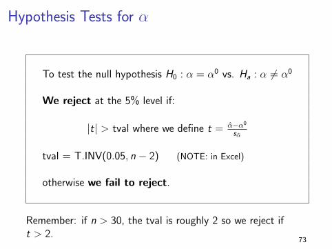
Hypothesis Tests for α
To test the null hypothesis H0 : α = α0 vs. Ha : α 6= α0
We reject at the 5% level if:
|t| > tval where we define t = α−α0
sα
tval = T.INV(0.05, n − 2) (NOTE: in Excel)
otherwise we fail to reject.
Remember: if n > 30, the tval is roughly 2 so we reject ift > 2.
73
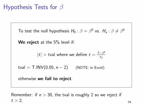
Hypothesis Tests for β
To test the null hypothesis H0 : β = β0 vs. Ha : β 6= β0
We reject at the 5% level if:
|t| > tval where we define t = β−β0
sβ
tval = T.INV(0.05, n − 2) (NOTE: in Excel)
otherwise we fail to reject.
Remember: if n > 30, the tval is roughly 2 so we reject ift > 2. 74
Hypothesis Tests for β
IMPORTANT: The null hypothesis that:
H0 : β = 0
plays a very important role in regression analysis.
Why?
Remember, the conditional distribution of Y is
Y |X = x ∼ N(α + βx , σ2)
Consequently, if β = 0 then the conditional distribution of Ydoes not depend on X . This means that the random variablesY and X are independent (at least according to our model)!!
75
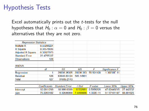
Hypothesis Tests
Excel automatically prints out the t-tests for the nullhypotheses that H0 : α = 0 and H0 : β = 0 versus thealternatives that they are not zero.
76
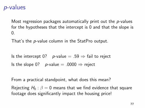
p-values
Most regression packages automatically print out the p-valuesfor the hypotheses that the intercept is 0 and that the slope is0.
That’s the p-value column in the StatPro output.
Is the intercept 0? p-value = .59 ⇒ fail to reject
Is the slope 0? p-value = .0000 ⇒ reject
From a practical standpoint, what does this mean?
Rejecting H0 : β = 0 means that we find evidence that squarefootage does significantly impact the housing price!
77
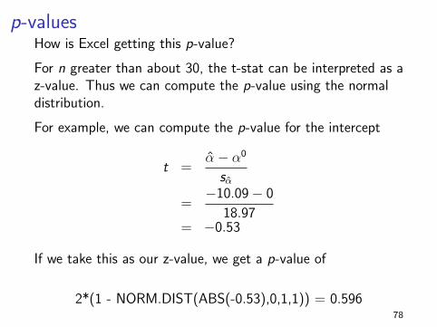
p-valuesHow is Excel getting this p-value?
For n greater than about 30, the t-stat can be interpreted as az-value. Thus we can compute the p-value using the normaldistribution.
For example, we can compute the p-value for the intercept
t =α− α0
sα
=−10.09− 0
18.97= −0.53
If we take this as our z-value, we get a p-value of
2*(1 - NORM.DIST(ABS(-0.53),0,1,1)) = 0.59678
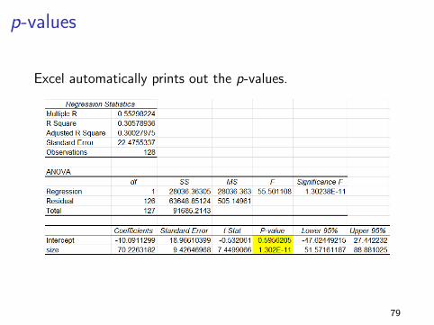
p-values
Excel automatically prints out the p-values.
79
Fits, residuals, and R-squared
80
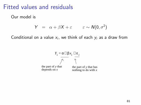
Fitted values and residuals
Our model is
Y = α + βX + ε ε ∼ N(0, σ2)
Conditional on a value xi , we think of each yi as a draw from
Yi = α+ β xi + ε i
the part of y that depends on x
the part of y that has nothing to do with x
81
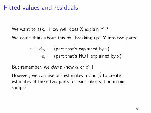
Fitted values and residuals
We want to ask, “How well does X explain Y”?
We could think about this by “breaking up” Y into two parts:
α + βxi (part that’s explained by x)
εi (part that’s NOT explained by x)
But remember, we don’t know α or β !!
However, we can use our estimates α and β to createestimates of these two parts for each observation in oursample.
82
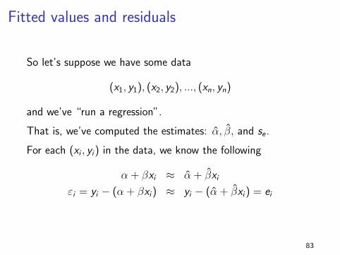
Fitted values and residuals
So let’s suppose we have some data
(x1, y1), (x2, y2), ..., (xn, yn)
and we’ve “run a regression”.
That is, we’ve computed the estimates: α, β, and se .
For each (xi , yi) in the data, we know the following
α + βxi ≈ α + βxi
εi = yi − (α + βxi) ≈ yi − (α + βxi) = ei
83
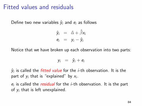
Fitted values and residuals
Define two new variables yi and ei as follows
yi = α + βxi
ei = yi − yi
Notice that we have broken up each observation into two parts:
yi = yi + ei
yi is called the fitted value for the i -th observation. It is thepart of yi that is “explained” by xi .
ei is called the residual for the i -th observation. It is the partof yi that is left unexplained.
84
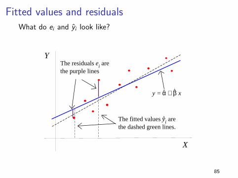
Fitted values and residualsWhat do ei and yi look like?
X
Y
y = α + β x
The residuals ei are the purple lines
The fitted values yi are the dashed green lines.
85
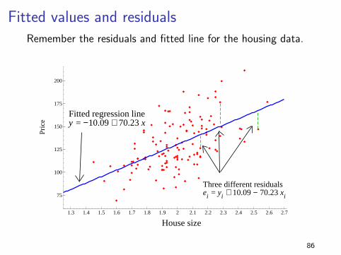
Fitted values and residualsRemember the residuals and fitted line for the housing data.
1.3 1.4 1.5 1.6 1.7 1.8 1.9 2 2.1 2.2 2.3 2.4 2.5 2.6 2.7
75
100
125
150
175
200
Pric
e
House size
Fitted regression line y = −10.09 + 70.23 x
Three different residualsei = yi + 10.09 − 70.23 xi
86
Least squares interpretation
We stated earlier that α and β are often called the leastsquares estimates of α and β.
The line we are fitting through the data is the “best fitting”line because α and β are chosen to minimize the function
SSR =n∑
i=1
(yi − α− βxi
)2where SSR stands for the sum of squared residuals.
A by-product of this is that by construction our residuals eiwill have “nice properties.”
87
Properties of the residual
Two important properties of the residuals ei are:
I The sample mean of the residuals equals zero:e = 1
n
∑ni=1 ei = 0.
I The sample correlation between the residuals e and theexplanatory variable x is zero: cor(e, x) = 0.
Let’s see what this looks like graphically on the housing data.
88
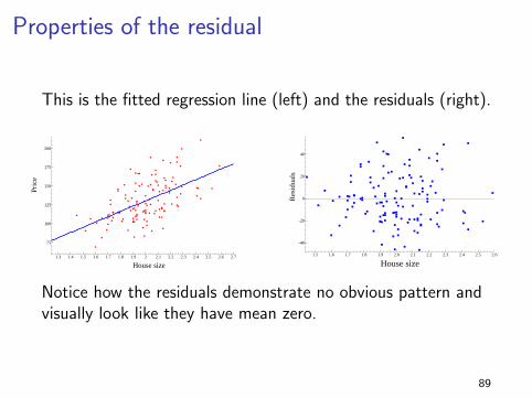
Properties of the residual
This is the fitted regression line (left) and the residuals (right).
1.3 1.4 1.5 1.6 1.7 1.8 1.9 2 2.1 2.2 2.3 2.4 2.5 2.6 2.7
75
100
125
150
175
200
Pric
e
House size
1.5 1.6 1.7 1.8 1.9 2.0 2.1 2.2 2.3 2.4 2.5 2.6
-40
-20
0
20
40
Res
idua
ls
House size
Notice how the residuals demonstrate no obvious pattern andvisually look like they have mean zero.
89
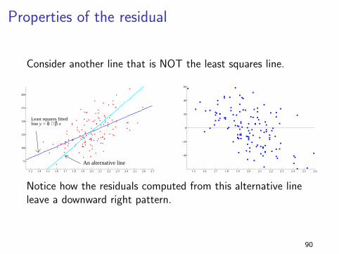
Properties of the residual
Consider another line that is NOT the least squares line.
1.3 1.4 1.5 1.6 1.7 1.8 1.9 2.0 2.1 2.2 2.3 2.4 2.5 2.6 2.7
75
100
125
150
175
200
Least squares fitted line y = α + β x
An alternative line1.5 1.6 1.7 1.8 1.9 2.0 2.1 2.2 2.3 2.4 2.5 2.6
−40
−20
0
20
40
60
Notice how the residuals computed from this alternative lineleave a downward right pattern.
90
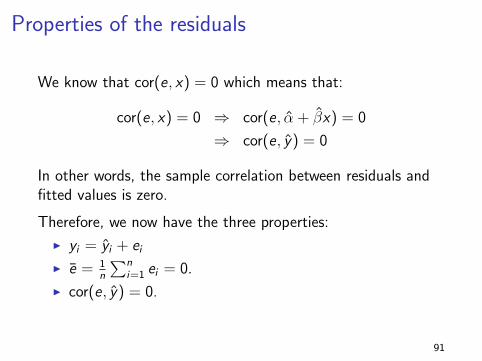
Properties of the residuals
We know that cor(e, x) = 0 which means that:
cor(e, x) = 0 ⇒ cor(e, α + βx) = 0
⇒ cor(e, y) = 0
In other words, the sample correlation between residuals andfitted values is zero.
Therefore, we now have the three properties:
I yi = yi + eiI e = 1
n
∑ni=1 ei = 0.
I cor(e, y) = 0.
91
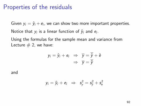
Properties of the residuals
Given yi = yi + ei , we can show two more important properties.
Notice that yi is a linear function of yi and ei .
Using the formulas for the sample mean and variance fromLecture # 2, we have:
yi = yi + ei ⇒ y = y + e
⇒ y = y
and
yi = yi + ei ⇒ s2y = s2y + s2e
92
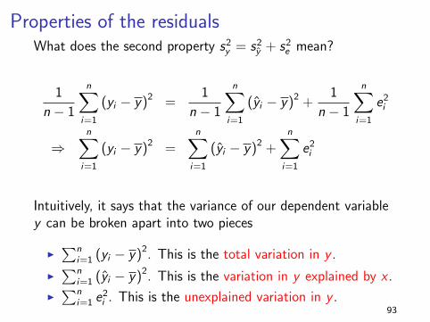
Properties of the residualsWhat does the second property s2y = s2y + s2e mean?
1
n − 1
n∑i=1
(yi − y)2 =1
n − 1
n∑i=1
(yi − y)2 +1
n − 1
n∑i=1
e2i
⇒n∑
i=1
(yi − y)2 =n∑
i=1
(yi − y)2 +n∑
i=1
e2i
Intuitively, it says that the variance of our dependent variabley can be broken apart into two pieces
I∑n
i=1 (yi − y)2. This is the total variation in y .
I∑n
i=1 (yi − y)2. This is the variation in y explained by x .
I∑n
i=1 e2i . This is the unexplained variation in y .
93
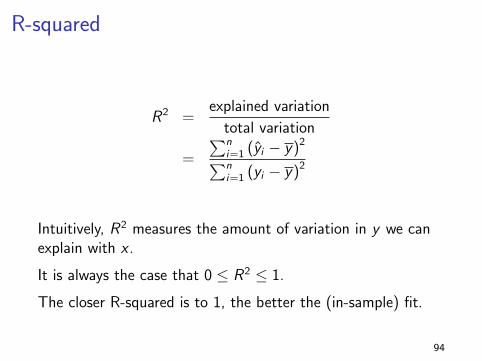
R-squared
R2 =explained variation
total variation
=
∑ni=1 (yi − y)2∑ni=1 (yi − y)2
Intuitively, R2 measures the amount of variation in y we canexplain with x .
It is always the case that 0 ≤ R2 ≤ 1.
The closer R-squared is to 1, the better the (in-sample) fit.
94
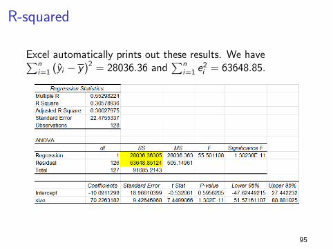
R-squared
Excel automatically prints out these results. We have∑ni=1 (yi − y)2 = 28036.36 and
∑ni=1 e2
i = 63648.85.
95
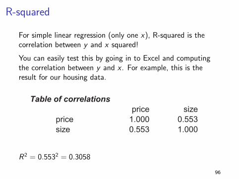
R-squared
For simple linear regression (only one x), R-squared is thecorrelation between y and x squared!
You can easily test this by going in to Excel and computingthe correlation between y and x . For example, this is theresult for our housing data.
Table of correlations
price size
price 1.000 0.553
size 0.553 1.000
R2 = 0.5532 = 0.3058
96
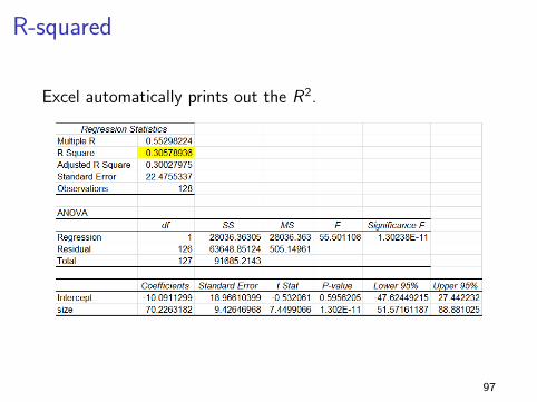
R-squared
Excel automatically prints out the R2.
97

Application: The Market Model
98
The Market Model
In finance, a popular model is to regress stock returns againstreturns on some market index, such as the S&P 500.
The slope of the regression line, referred to as “beta”, is ameasure of how sensitive a stock is to movements in themarket.
Usually, a beta less than 1 means the stock is less risky thanthe market, equal to 1 same risk as the market and greaterthan 1, riskier than the market.
99
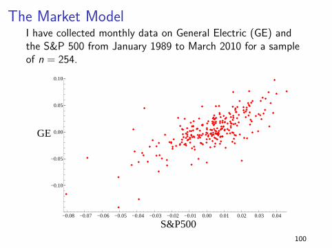
The Market ModelI have collected monthly data on General Electric (GE) andthe S&P 500 from January 1989 to March 2010 for a sampleof n = 254.
−0.08 −0.07 −0.06 −0.05 −0.04 −0.03 −0.02 −0.01 0.00 0.01 0.02 0.03 0.04
−0.10
−0.05
0.00
0.05
0.10
GE
S&P500100
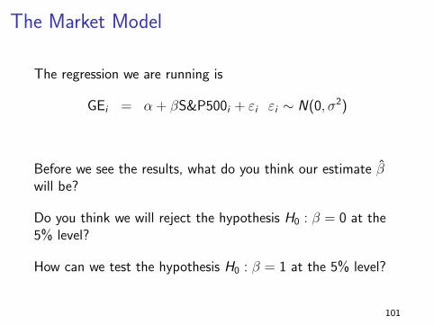
The Market Model
The regression we are running is
GEi = α + βS&P500i + εi εi ∼ N(0, σ2)
Before we see the results, what do you think our estimate βwill be?
Do you think we will reject the hypothesis H0 : β = 0 at the5% level?
How can we test the hypothesis H0 : β = 1 at the 5% level?
101
The Market Model
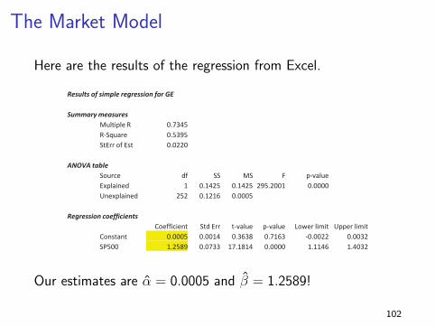
Here are the results of the regression from Excel.
Results of simple regression for GE
Summary measures
Multiple R 0.7345
R-Square 0.5395
StErr of Est 0.0220
ANOVA table
Source df SS MS F p-value
Explained 1 0.1425 0.1425 295.2001 0.0000
Unexplained 252 0.1216 0.0005
Regression coefficients
Coefficient Std Err t-value p-value Lower limit Upper limit
Constant 0.0005 0.0014 0.3638 0.7163 -0.0022 0.0032
SP500 1.2589 0.0733 17.1814 0.0000 1.1146 1.4032
Our estimates are α = 0.0005 and β = 1.2589!
102
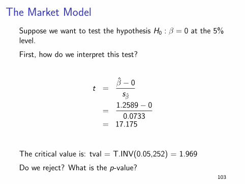
The Market Model
Suppose we want to test the hypothesis H0 : β = 0 at the 5%level.
First, how do we interpret this test?
t =β − 0
sβ
=1.2589− 0
0.0733= 17.175
The critical value is: tval = T.INV(0.05,252) = 1.969
Do we reject? What is the p-value?103
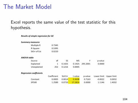
The Market Model
Excel reports the same value of the test statistic for thishypothesis.
Results of simple regression for GE
Summary measures
Multiple R 0.7345
R-Square 0.5395
StErr of Est 0.0220
ANOVA table
Source df SS MS F p-value
Explained 1 0.1425 0.1425 295.2001 0.0000
Unexplained 252 0.1216 0.0005
Regression coefficients
Coefficient Std Err t-value p-value Lower limit Upper limit
Constant 0.0005 0.0014 0.3638 0.7163 -0.0022 0.0032
SP500 1.2589 0.0733 17.1814 0.0000 1.1146 1.4032
104

The Market Model
Suppose we want to test the hypothesis H0 : β = 1 at the 5%level.
First, how do we interpret this test?
t =β − 1
sβ
=1.2589− 1
0.0733= 3.53
The critical value is: tval = T.INV(0.05,252) = 1.969
Do we reject the hypothesis?105
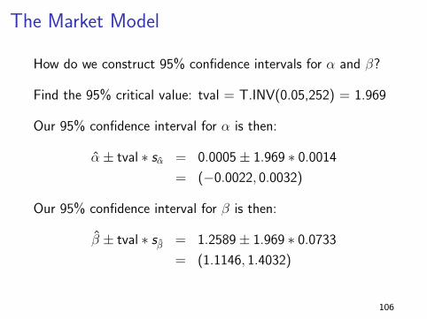
The Market Model
How do we construct 95% confidence intervals for α and β?
Find the 95% critical value: tval = T.INV(0.05,252) = 1.969
Our 95% confidence interval for α is then:
α± tval ∗ sα = 0.0005± 1.969 ∗ 0.0014
= (−0.0022, 0.0032)
Our 95% confidence interval for β is then:
β ± tval ∗ sβ = 1.2589± 1.969 ∗ 0.0733
= (1.1146, 1.4032)
106
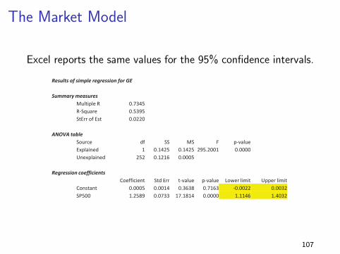
The Market Model
Excel reports the same values for the 95% confidence intervals.
Results of simple regression for GE
Summary measures
Multiple R 0.7345
R-Square 0.5395
StErr of Est 0.0220
ANOVA table
Source df SS MS F p-value
Explained 1 0.1425 0.1425 295.2001 0.0000
Unexplained 252 0.1216 0.0005
Regression coefficients
Coefficient Std Err t-value p-value Lower limit Upper limit
Constant 0.0005 0.0014 0.3638 0.7163 -0.0022 0.0032
SP500 1.2589 0.0733 17.1814 0.0000 1.1146 1.4032
107
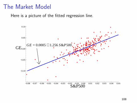
The Market ModelHere is a picture of the fitted regression line.
−0.08 −0.07 −0.06 −0.05 −0.04 −0.03 −0.02 −0.01 0.00 0.01 0.02 0.03 0.04 0.05
−0.10
−0.05
0.00
0.05
0.10
GE
S&P500
GE = 0.0005 + 1.256 S&P500
108

The Market ModelHere is a picture of the residuals.
−0.08 −0.07 −0.06 −0.05 −0.04 −0.03 −0.02 −0.01 0.00 0.01 0.02 0.03 0.04
−0.075
−0.050
−0.025
0.000
0.025
0.050
0.075
ei
S&P500
109


![©2014 Check Point Software Technologies Ltd. 41000 Introduction [Confidential] For designated groups and individuals](https://img.pdfslide.net/doc/110x75/56649ea25503460f94ba60ac/2014-check-point-software-technologies-ltd-41000-introduction-confidential.jpg)