Embed Size (px)
Citation preview

Business Statistics: A First Course, 5e © 2009 Prentice-Hall, Inc. Chap 12-1
Correlation and Regression
Business Statistics: A First Course, 5e © 2009 Prentice-Hall, Inc.. Chap 12-2
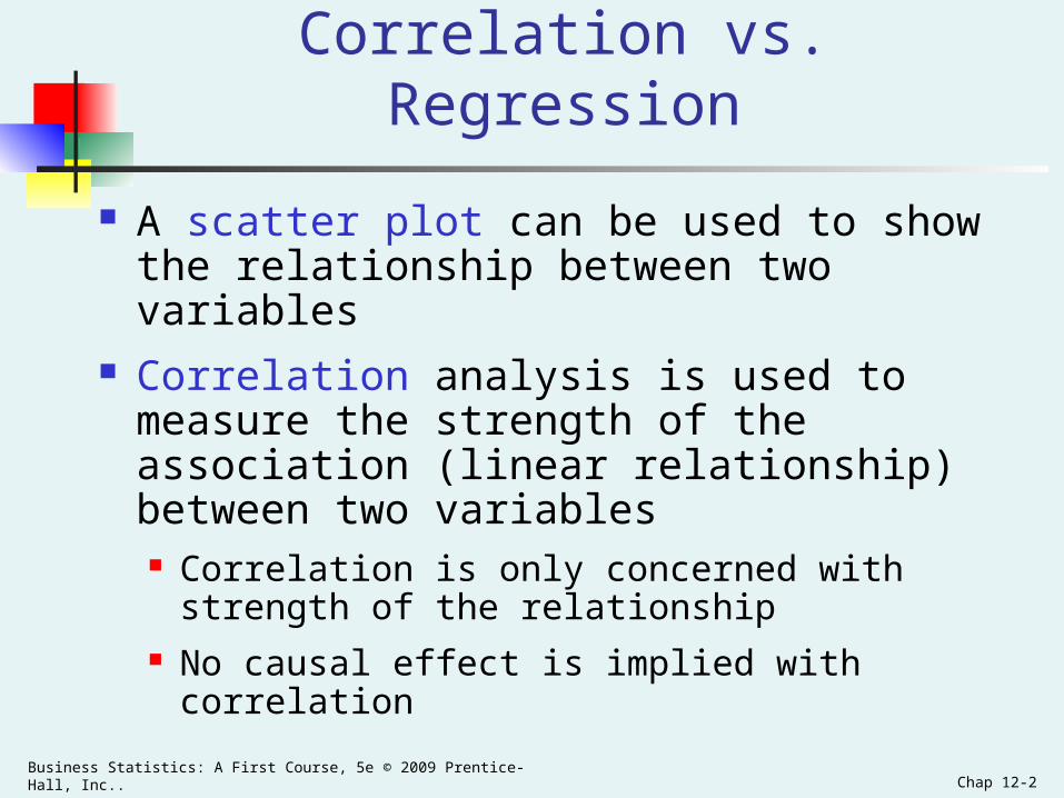
Correlation vs. Regression
A scatter plot can be used to show the relationship between two variables
Correlation analysis is used to measure the strength of the association (linear relationship) between two variables Correlation is only concerned with strength of the
relationship No causal effect is implied with correlation

Business Statistics: A First Course, 5e © 2009 Prentice-Hall, Inc.. Chap 12-3
Introduction to Regression Analysis
Regression analysis is used to: Predict the value of a dependent variable based on
the value of at least one independent variable Explain the impact of changes in an independent
variable on the dependent variable
Dependent variable: the variable we wish to predict or explain
Independent variable: the variable used to predict or explain the dependent
variable

Business Statistics: A First Course, 5e © 2009 Prentice-Hall, Inc.. Chap 12-4
Simple Linear Regression Model
Only one independent variable, X
Relationship between X and Y is described by a linear function
Changes in Y are assumed to be related to changes in X

Business Statistics: A First Course, 5e © 2009 Prentice-Hall, Inc. Chap 3-5
Scatter Plots of Sample Data with Various Coefficients of Correlation
Y
X
Y
X
Y
X
Y
X
r = -1 r = -.6
r = +.3r = +1
Y
Xr = 0

Business Statistics: A First Course, 5e © 2009 Prentice-Hall, Inc.. Chap 12-6
Types of Relationships
Y
X
Y
X
Y
Y
X
X
Linear relationships Curvilinear relationships
Business Statistics: A First Course, 5e © 2009 Prentice-Hall, Inc.. Chap 12-7
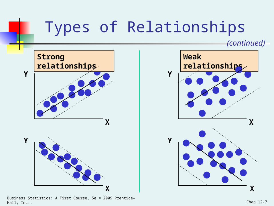
Types of Relationships
Y
X
Y
X
Y
Y
X
X
Strong relationships Weak relationships
(continued)

Business Statistics: A First Course, 5e © 2009 Prentice-Hall, Inc.. Chap 12-8
Types of Relationships
Y
X
Y
X
No relationship
(continued)

Business Statistics: A First Course, 5e © 2009 Prentice-Hall, Inc.. Chap 12-9
ii10i εXββY Linear component
Simple Linear Regression Model
Population Y intercept
Population SlopeCoefficient
Random Error term
Dependent Variable
Independent Variable
Random Error component

Business Statistics: A First Course, 5e © 2009 Prentice-Hall, Inc.. Chap 12-10
(continued)
Random Error for this Xi value
Y
X
Observed Value of Y for Xi
Predicted Value of Y for Xi
ii10i εXββY
Xi
Slope = β1
Intercept = β0
εi
Simple Linear Regression Model
Business Statistics: A First Course, 5e © 2009 Prentice-Hall, Inc.. Chap 12-11
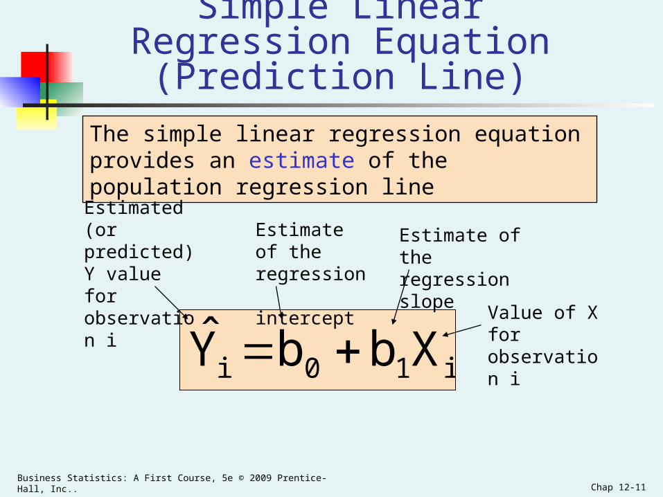
i10i XbbY
The simple linear regression equation provides an estimate of the population regression line
Simple Linear Regression Equation (Prediction Line)
Estimate of the regression
intercept
Estimate of the regression slope
Estimated (or predicted) Y value for observation i
Value of X for observation i

Business Statistics: A First Course, 5e © 2009 Prentice-Hall, Inc.. Chap 12-12
b0 is the estimated mean value of Y
when the value of X is zero
b1 is the estimated change in the mean
value of Y as a result of a one-unit change in X
Interpretation of the Slope and the Intercept

Business Statistics: A First Course, 5e © 2009 Prentice-Hall, Inc.. Chap 12-13
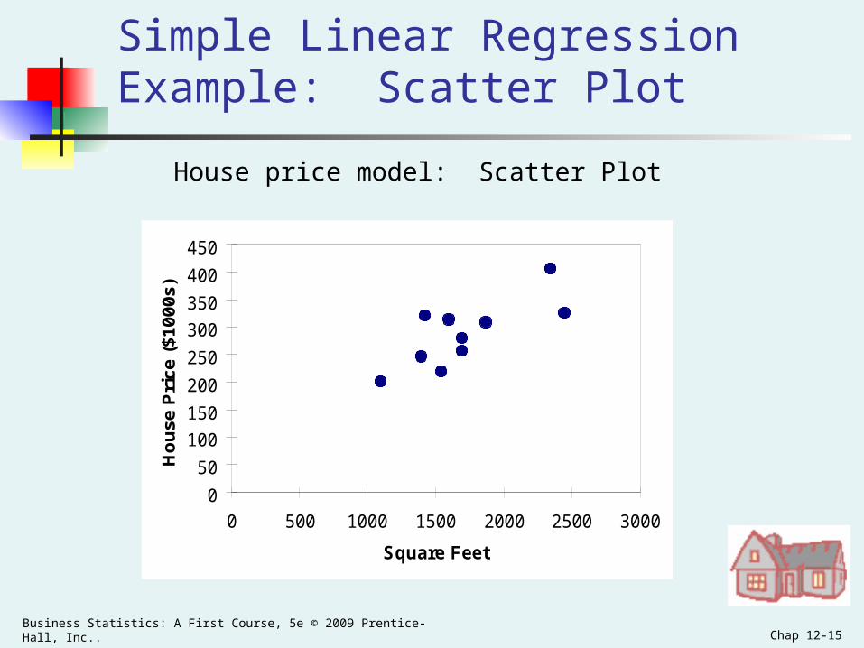
Simple Linear Regression Example
A real estate agent wishes to examine the relationship between the selling price of a home and its size (measured in square feet)
A random sample of 10 houses is selected Dependent variable (Y) = house price in $1000s Independent variable (X) = square feet

Business Statistics: A First Course, 5e © 2009 Prentice-Hall, Inc.. Chap 12-14
Simple Linear Regression Example: Data
House Price in $1000s(Y)
Square Feet (X)
245 1400
312 1600
279 1700
308 1875
199 1100
219 1550
405 2350
324 2450
319 1425
255 1700
Business Statistics: A First Course, 5e © 2009 Prentice-Hall, Inc.. Chap 12-15
0
50
100
150
200
250
300
350
400
450
0 500 1000 1500 2000 2500 3000
Square Feet
Ho
use
Pri
ce (
$100
0s)
Simple Linear Regression Example: Scatter Plot
House price model: Scatter Plot

Business Statistics: A First Course, 5e © 2009 Prentice-Hall, Inc.. Chap 12-16
Simple Linear Regression Example: Using Excel

Business Statistics: A First Course, 5e © 2009 Prentice-Hall, Inc.. Chap 12-17
Simple Linear Regression Example: Excel Output
Regression Statistics
Multiple R 0.76211
R Square 0.58082
Adjusted R Square 0.52842
Standard Error 41.33032
Observations 10
ANOVA df SS MS F Significance F
Regression 1 18934.9348 18934.9348 11.0848 0.01039
Residual 8 13665.5652 1708.1957
Total 9 32600.5000
Coefficients Standard Error t Stat P-value Lower 95% Upper 95%
Intercept 98.24833 58.03348 1.69296 0.12892 -35.57720 232.07386
Square Feet 0.10977 0.03297 3.32938 0.01039 0.03374 0.18580
The regression equation is:
feet) (square 0.10977 98.24833 price house

Business Statistics: A First Course, 5e © 2009 Prentice-Hall, Inc.. Chap 12-18
Simple Linear Regression Example: Minitab Output
The regression equation is
Price = 98.2 + 0.110 Square Feet Predictor Coef SE Coef T PConstant 98.25 58.03 1.69 0.129Square Feet 0.10977 0.03297 3.33 0.010 S = 41.3303 R-Sq = 58.1% R-Sq(adj) = 52.8% Analysis of Variance Source DF SS MS F PRegression 1 18935 18935 11.08 0.010Residual Error 8 13666 1708Total 9 32600
The regression equation is:
house price = 98.24833 + 0.10977 (square feet)

Business Statistics: A First Course, 5e © 2009 Prentice-Hall, Inc.. Chap 12-19
0
50
100
150
200
250
300
350
400
450
0 500 1000 1500 2000 2500 3000
Square Feet
Ho
use
Pri
ce (
$100
0s)
Simple Linear Regression Example: Graphical Representation
House price model: Scatter Plot and Prediction Line
feet) (square 0.10977 98.24833 price house
Slope = 0.10977
Intercept = 98.248
Business Statistics: A First Course, 5e © 2009 Prentice-Hall, Inc.. Chap 12-20
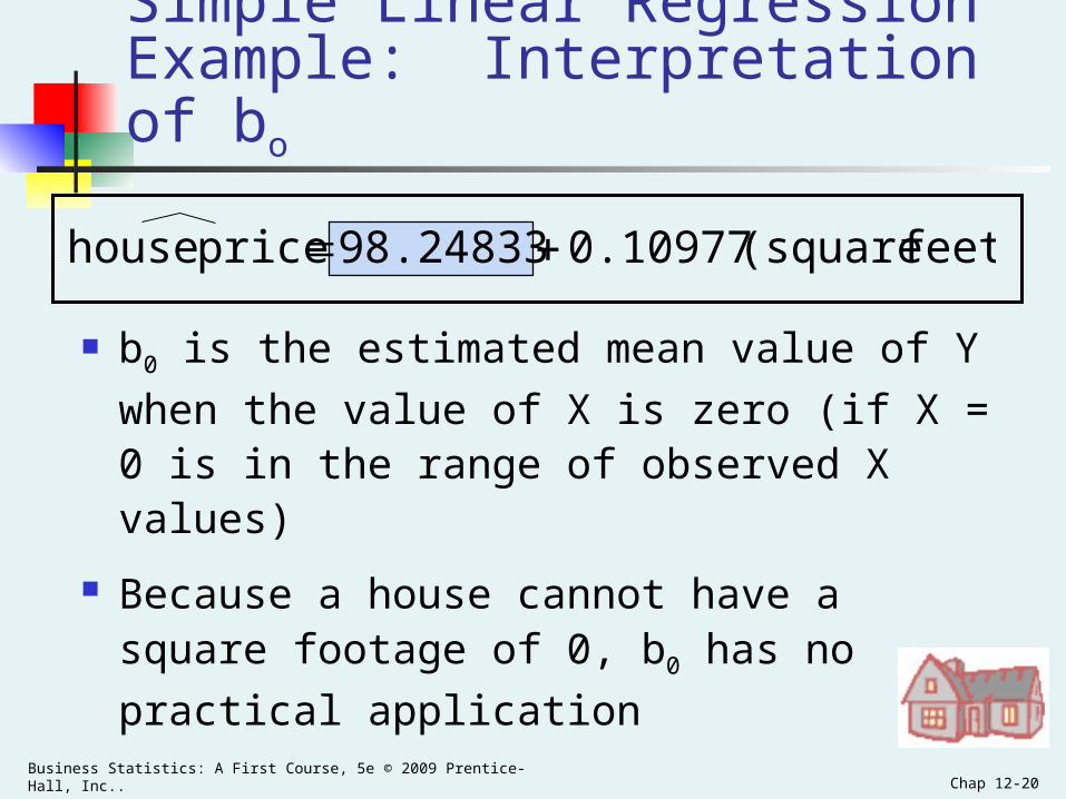
Simple Linear Regression Example: Interpretation of bo
b0 is the estimated mean value of Y when the
value of X is zero (if X = 0 is in the range of observed X values)
Because a house cannot have a square footage of 0, b0 has no practical application
feet) (square 0.10977 98.24833 price house

Business Statistics: A First Course, 5e © 2009 Prentice-Hall, Inc.. Chap 12-21
Simple Linear Regression Example: Interpreting b1
b1 estimates the change in the mean
value of Y as a result of a one-unit increase in X Here, b1 = 0.10977 tells us that the mean value of a
house increases by 0.10977($1000) = $109.77, on average, for each additional one square foot of size
feet) (square 0.10977 98.24833 price house

Business Statistics: A First Course, 5e © 2009 Prentice-Hall, Inc.. Chap 12-22
317.85
0)0.1098(200 98.25
(sq.ft.) 0.1098 98.25 price house
Predict the price for a house with 2000 square feet:
The predicted price for a house with 2000 square feet is 317.85($1,000s) = $317,850
Simple Linear Regression Example: Making Predictions