Embed Size (px)
Citation preview

BUSINESS STATISTICS Assignment Submitted to Dr.R Venkata Muni Reddy 9/24/2009
Alliance Business School
Submitted By
GROUP 2:
Abhishek Modi (09PG266)
Ayushee Singh (09PG251)
Kanika Setia (09PG261)
Paras Kumar (09PG271)
Rohit Tomar (09PG281)
Sugandha Huria (09PG291)

Business Statistics September 24, 2009
Alliance Business School, Bangalore Page 2
INTRODUCTION AND BASIC CONCEPTS
Statistics is a mathematical science pertaining to the collection, analysis, interpretation or
explanation, and presentation of data. Statisticians improve the quality of data with the design of
experiments and survey sampling. Statistics also provides tools for prediction and forecasting
using data and statistical models. Statistics is applicable to a wide variety of academic
disciplines, including natural and social sciences, government, and business.
Statistical methods can be used to summarize or describe a collection of data; this is called
descriptive statistics. This is useful in research, when communicating the results of experiments.
In addition, patterns in the data may be modeled in a way that accounts for randomness and
uncertainty in the observations, and are then used to draw inferences about the process or
population being studied; this is called inferential statistics. Inference is a vital element of
scientific advance, since it provides a prediction (based in data) for where a theory logically
leads. To further prove the guiding theory, these predictions are tested as well, as part of the
scientific method. If the inference holds true, then the descriptive statistics of the new data
increase the soundness of that hypothesis. Descriptive statistics and inferential statistics (a.k.a.,
predictive statistics) together comprise applied statistics.
There is also a discipline called mathematical statistics, which is concerned with the theoretical
basis of the subject
Statistics is about gaining information from sets of data. Sometimes you want to represent a lot
of complicated information from a large data set in a way that is easily understood. This is called
descriptive statistics.
Statistics is about gaining information from sets of data. Sometimes you want to represent a lot
of complicated information from a large data set in a way that is easily understood. This is called
descriptive statistics.
An example of this is the so-called worm plot used in cricket: over the cause of a cricket match
there can be many hundreds of balls and runs. In the worm plot depicted below, England‘s
performance is described by the blue line and the West Indies‘ by the green line. You can see at a

Business Statistics September 24, 2009
Alliance Business School, Bangalore Page 3
glance that, although there was variation in the run rate, England consistently scored at a higher
rate than the West Indies, and so won the match.
Although some information has been lost - you don't know for instance from which balls in the
overs runs were taken - this summary graph clearly displays all of the meaningful information.
The human mind is very visual, and this is why graphics, such as graphs or pie charts, are very
good for conveying statistical information.
The other branch of statistics is called inference statistics. This used to obtain information about
a large set of data from a smaller sample. Think of opinion polls. Here, the statistician randomly
selects a group of people, a thousand say, and asks them about their opinion, for example
whether or not they like the current government. It is then assumed that the opinion of the sample
reflects the opinions of people as a whole.
To be able to do statistics, you first have to learn how to collect, handle and represent data.
USE OF STATISTICAL DATA
Probability theory
Statistics is intimately linked to probability theory. You can use statistics to work out the
probability, the chance that a certain event will occur: if you want to know the chance that your
holiday plane will crash, you think of how many planes usually crash within a year. Since this
number is very small, you deduce that the chance of your plane crashing is small also. You've
done a very simple statistical analysis of the data concerning plane crashes and used it to work
out a probability.
But things also work the other way around: you can use abstract probabilities to help you with
your stats. Say for example you want to test whether a die that is used in a casino is fair. To do

Business Statistics September 24, 2009
Alliance Business School, Bangalore Page 4
this, you throw the die a great number of times and record the outcomes. You then reason like
this: if the die is fair, then each number should be equally likely. There are six numbers, so each
number should come up in 1/6 of the cases. If this is the case, you decide that it is fair.
This example shows how the abstract theory of probability can help to evaluate real-life
statistics. And this is why probability theory belongs to the basic tool set of a statistician.
So who, apart from opinion pollsters and professional gamblers, uses statistics? Here are a few
examples:
Medicine
Stats and probability theory are absolutely essential in medicine as they are used to test new
drugs and work out the chance that patients develop side effects from the drugs. Tests are
performed on large groups of animals or people and stats are the tool needed to evaluate the tests.
It's essential to get it right, for obvious reasons. Even doctors and nurses who don't perform the
tests themselves need to be well-versed in stats to understand the results and advise their patients
accurately.
Stats and probability theory are also used to assess the risk from things like tobacco and alcohol,
and to see how a certain gene affects people. How likely is it that a person with that gene
develops a certain illness or characteristic?
Medical research cannot do without statistics.
Social and natural sciences
On the face of it, sciences like psychology, sociology or biology do not seem to have much to do
with maths or stats. But all of these have one thing in common: they are based on observations of
the world around us. A psychologist might want to observe people with a certain mental illness, a
biologist the behavior of a virus, and a sociologist a possible link between criminality and drug
abuse. To evaluate these observations, scientists need descriptive statistics. They need to know
how to best collect data and how to represent them in a meaningful way. To interpret the data,
they need inference statistics.

Business Statistics September 24, 2009
Alliance Business School, Bangalore Page 5
The financial world
A very important thing in the financial world is risk assessment: what is the probability, or risk,
of a company going bankrupt, or the interest rates going up? What is the risk of investing in a
company, or of taking on a mortgage? The insurance industry is based on the idea of risk: the
chance of your house burning down is quite small, but if it does happen, you lose everything.
The insurance company exactly balances the risk of fire with the cost of a fire. They decide what
premium to charge you, so that they still make a profit even though they sometimes pay out huge
amounts.
A good understanding of risk and how it can be described using statistics and probability, is
essential for anyone working in the financial world. Employers in this area often value
mathematicians and statisticians just as highly as people with an economics background.
Politics
Politics is very much about strategy. How should an election campaign be fought? How should a
government deal with other powers? How much money should the health service receive? To
find a good strategy, politicians need to understand public opinion, know about the structure of
society and assess risks. The government employs many statisticians to help them with this. They
can conduct and evaluate a census, and work out the risk of there being an epidemic, or of the
world economy plunging.
During the cold war, game theory, which is closely related to probability theory, was used to
decide whether the US strategy - arming itself to the teeth to deter an attack from the USSR -
was effective.
Reliability theory in manufacturing
When you produce a product, be it a car or a light bulb, you want to know how reliable it is. To
find out, you take a sample of your light bulbs or cars and test them. Just as in an opinion poll,
you can use statistical methods to gain information about the quality of your product from this
sample. Reliability theory has become a very important branch within statistics.
Business Statistics September 24, 2009
Alliance Business School, Bangalore Page 6
Law
Statistics is often used in the courts. Say a DNA sample has been taken from a crime scene. What
is the chance that a defendant matches this DNA even though he or she is innocent?
In fact, the use of statistics in court can be very tricky, because people are easily confused by it.
A few years ago, a woman called Sally Clark was jailed for the murder of her two children. She
said that they both died of cot death, but the jury was told by an "expert witness" that the
probability of two children dying of cot death in the same family is extremely low, so they
decided that she must have killed them. But this reasoning is flawed. This was recognized later
and the woman was eventually released.
All of us
Everyday life is full of statistics that we need to understand. Politicians and commercial
organizations use stats to convince us to vote for them or buy their products. We need stats to
understand the risks involved in taking a certain medicine or making financial decisions. A basic
grasp of statistics means that you don't have to rely on someone else to make up your mind about
these things. You don‘t need to be an expert — a little basic knowledge can go a long way in
understanding the numbers you are bombarded with every day.
Business Statistics:
The word ‗statistics‘ is derived from the Latin word ‗status‘ meaning a political state. In those
days, therefore, statistics was simply the collection of numerical data by the state or kings. Now,
statistics is the scientific method of analyzing quantitative information. It includes methods of
collection, classification, description and interpretation of data. It simply refers to numerical
description of the quantitative aspects of a phenomenon.
Definition: By statistics we mean aggregate of facts affected to a marked extent by multiplicity
of causes numerically expressed, enumerated or estimated according to reasonable standards of
accuracy, collected in a systematic manner for a predetermined purpose and placed in relation to
each other. Or it can also be defines as a science of collection, presentation, analysis and
interpretation of numerical data.
Raw Data Raw data represent numbers and facts in the original format in which data have been collected
Example for raw data: Z
Business Statistics September 24, 2009
Alliance Business School, Bangalore Page 7
Frequency Distribution
Frequency Distribution is a summarized table in which raw data are arranged into classes and
frequencies. It is called grouped data. The grouped data can be classified into two. They are
discrete data and continuous data.
Discrete data Discrete data can take only certain specific values that are whole numbers. Example: Number of
classrooms in a school, number of students in a class. Discrete numbers cannot take fractional
values.
Continuous data
Continuous data can take any numerical value within a specific interval e.g. height in
centimeters; weight in kilograms; income in rupees.
Sources of Data
There are two basic sources of collecting the data. They are (i) Primary source and (ii) Secondary
source. If the data are collected from primary source, it is called primary data. The data collected
from the secondary sources are called the secondary data.
Primary data
Data collected for the first time for a specific purpose is called primary data. They are original in
character. They are collected by individuals or institutions or government for research purpose or
policy decisions. Example: Data collected in a population census by the office of the census
commissioner.
Secondary Data
These data are not originally collected. They are obtained from published or unpublished
sources. Published sources are reports and official publications like annual reports of the bank,
population census, Economic survey of India; unpublished sources are the Government records,
studies made by research institutions. Example for the secondary data: Census data used by
research scholars. The census data are primary to the office of the census commissioner who
collected it and for others it is a secondary data.
Classification of Data
Classification is the process of arranging the collected data into classes and to subclasses
according to their common characteristics. Classification is the grouping of related facts into
classes. E.g. sorting of letters in post office

Business Statistics September 24, 2009
Alliance Business School, Bangalore Page 8
Types of classification
There are four types of classification. They are
(i) Geographical classification
(ii) Chronological classification
(iii) Qualitative classification
(iv) Quantitative classification
Types of Data
Two types of data: qualitative and quantitative. The way we typically define them, we call data
'quantitative' if it is in numerical form and 'qualitative' if it is not. Notice that qualitative data
could be much more than just words or text. Photographs, videos, sound recordings and so on,
can be considered qualitative data.
The quantitative types argue that their data is 'hard', 'rigorous', 'credible', and 'scientific'. The
qualitative proponents counter that their data is 'sensitive', 'nuanced', 'detailed', and 'contextual'.
The fact that qualitative and quantitative data are intimately related to each other. All
quantitative data is based upon qualitative judgments; and all qualitative data can be
described and manipulated numerically. For instance, think about a very common quantitative
measure in social research -- a self esteem scale. The researchers who develop such instruments
had to make countless judgments in constructing them: how to define self esteem; how to
distinguish it from other related concepts; how to word potential scale items; how to make sure
the items would be understandable to the intended respondents; what kinds of contexts it could
be used in; what kinds of cultural and language constraints might be present; and on and on. The
researcher who decides to use such a scale in their study has to make another set of judgments:
how well does the scale measure the intended concept; how reliable or consistent is it; how
appropriate is it for the research context and intended respondents; and on and on. Believe it or
not, even the respondents make many judgments when filling out such a scale: what is meant by

Business Statistics September 24, 2009
Alliance Business School, Bangalore Page 9
various terms and phrases; why is the researcher giving this scale to them; how much energy and
effort do they want to expend to complete it, and so on. Even the consumers and readers of the
research will make lots of judgments about the self esteem measure and its appropriateness in
that research context. What may look like a simple, straightforward, cut-and-dried quantitative
measure is actually based on lots of qualitative judgments made by lots of different people.
Quantitative and qualitative data are two types of data.
Qualitative data Qualitative - or categorical measurement expressed not in terms of numbers, but
rather by means of a natural language description. In statistics it is often used interchangeably
with "categorical" data.
For example: favourite colour = "blue"
height = "tall"
Although we may have categories, the categories may have a structure to them. When there is
not a natural ordering of the categories, we call these nominal categories. Examples might be
gender, race, religion, or sport.
When the categories may be ordered, these are called ordinal variables. Categorical variables
that judge size (small, medium, large, etc.) are ordinal variables. Attitudes (strongly disagree,
disagree, neutral, agree, strongly agree) are also ordinal variables, however we may not know
which value is the best or worst of these issues. Note that the distance between these categories is
not something we can measure.
Quantitative data
Quantitative -- or numerical measurement expressed not by means of a natural language
description, but rather in terms of numbers. However, not all numbers are continuous and
measurable -- for example social security number -- even though it is a number it is not
something that one can add or subtract.
For example: favourite colour = "450 nm"
height = "1.8 m"

Business Statistics September 24, 2009
Alliance Business School, Bangalore Page 10
Quantitative data always are associated with a scale measure.
Probably the most common scale type is the ratio-scale. Observations of this type are on a scale
that has a meaningful zero value but also have an equidistant measure (i.e., the difference
between 10 and 20 is the same as the difference between 100 and 110). For example a 10 year-
old girl is twice as old as a 5 year-old girl. Since you can measure zero years, time is a ratio-scale
variable. Money is another common ratio-scale quantitative measure. Observations that you
count are usually ratio-scale (e.g., number of widgets).
A more general quantitative measure is the interval scale. Interval scales also have a equidistant
measure. However, the doubling principle breaks down in this scale. A temperature of 50
degrees Celsius is not "half as hot" as a temperature of 100, but a difference of 10 degrees
indicates the same difference in temperature anywhere along the scale. The Kelvin temperature
scale, however, constitutes a ratio scale because on the Kelvin scale zero indicates absolute zero
in temperature, the complete absence of heat. So one can say, for example, that 200 degrees
Kelvin is twice as hot as 100 degrees Kelvin.

Business Statistics September 24, 2009
Alliance Business School, Bangalore Page 11
GRAPHICAL REPRESENTAION OF DATA

Business Statistics September 24, 2009
Alliance Business School, Bangalore Page 12

Business Statistics September 24, 2009
Alliance Business School, Bangalore Page 13

Business Statistics September 24, 2009
Alliance Business School, Bangalore Page 14

Business Statistics September 24, 2009
Alliance Business School, Bangalore Page 15

Business Statistics September 24, 2009
Alliance Business School, Bangalore Page 16

Business Statistics September 24, 2009
Alliance Business School, Bangalore Page 17
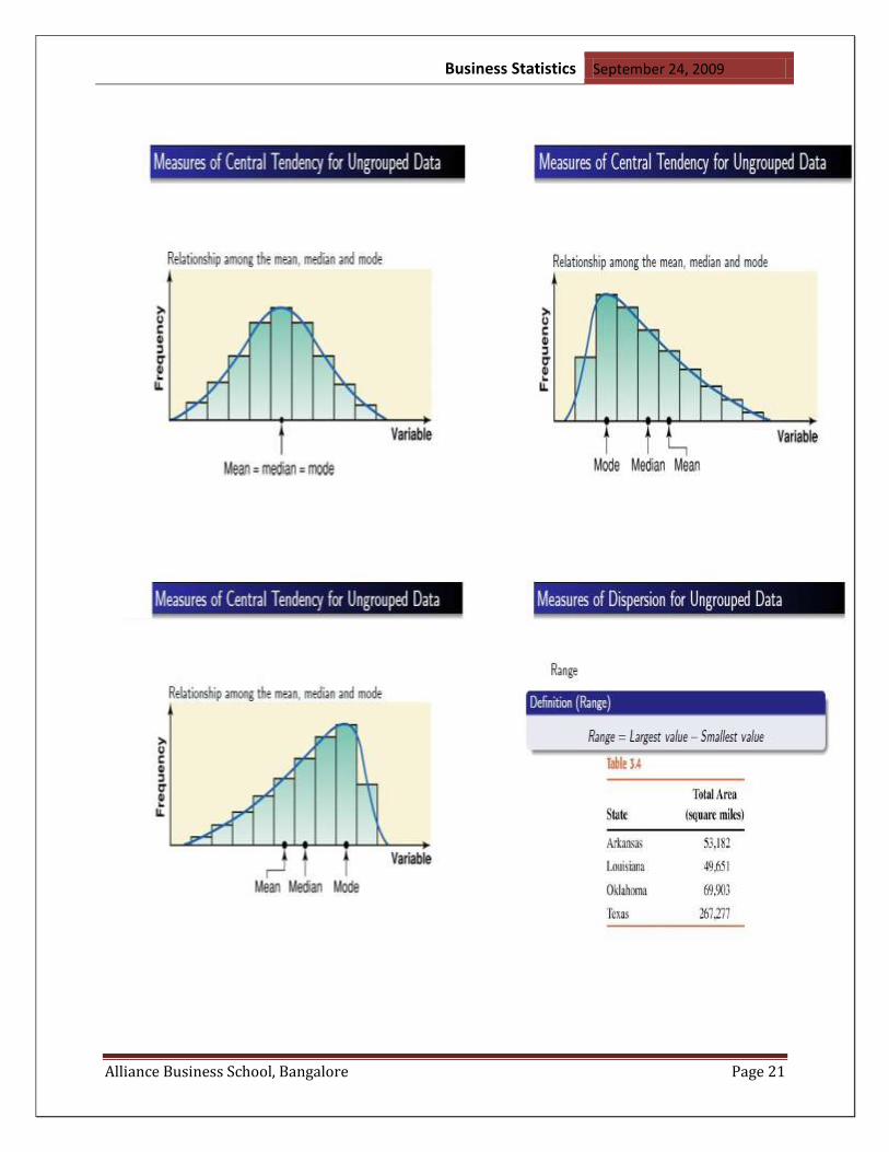
MEASURES OF CENTRAL TENDENCY
In analyzing, statistical data, it is often useful to have numbers describe the complete set of data.
―Measures of central tendency‖ are used because they represent centralized or middle values of
the data. These measures of central tendency are called the ―mean,‖ ―median,‖ and ―mode.‖
The ―mean‖ is a number that represents an ―average‖ of a set of data. It is found by adding the
elements in the set and then dividing that sum by the number of elements in the set.
Definition: The ―mean‖ of a set of data is the sum of the elements in the set divided by the
number of elements in the set.
Figure 1.1: Mean

Business Statistics September 24, 2009
Alliance Business School, Bangalore Page 18
Analysis of Mean in this example:
The mean temperature is greater than all of the daily temperatures except one, . Thus, is
not a very good representation of the average of the set of data? Extremely high or low values,
such as , affect the mean.
It must be pointed out that because the temperature is not a good representation of the set of
data, possibly the mean is not always the best average. This opens the door to introducing the
―median‖ and ―mode‖ as averages that sometimes are better representations.

Business Statistics September 24, 2009
Alliance Business School, Bangalore Page 19
The mode is the number that occurs most often in a set of data
A set of data may have more than one mode. For example, in {2, 3, 3, 4, 6, 6}, 3 and 6 are
both modes for the set of data. For a set in which there are two modes, it is sometimes said
to be bimodal, a set of three modes, trimodal, and so on. If no number occurs more often
than the other numbers, then a set of data has
no mode.

Business Statistics September 24, 2009
Alliance Business School, Bangalore Page 20
Median: The ―median‖ is the middle number of a set of data when the numbers are arranged in
increasing order.
2nd Example for MEDIAN:
If a set of data contains an even number of elements, the median is the value halfway
between the two middle elements. In other words, when there are an even number of
elements in a set of data, the median is found by determining the mean of the two middle
elements.
Business Statistics September 24, 2009
Alliance Business School, Bangalore Page 21

Business Statistics September 24, 2009
Alliance Business School, Bangalore Page 22
The Variance:
The variance of a set of observations is the average squared deviation of the data points from
their mean .This measure of dispersion reflects the values of all the measurements.
Solution of the above example :

Business Statistics September 24, 2009
Alliance Business School, Bangalore Page 23
Standard Deviation: A set of observations is the (positive) square root of the variance of set. the
standard deviation for a normal distribution is the distance along the horizontal axis between the
mean and either horizontal coordinate for which the curve changes concavity.

Business Statistics September 24, 2009
Alliance Business School, Bangalore Page 24

Business Statistics September 24, 2009
Alliance Business School, Bangalore Page 25

Business Statistics September 24, 2009
Alliance Business School, Bangalore Page 26
Example

Business Statistics September 24, 2009
Alliance Business School, Bangalore Page 27
Example
Business Statistics September 24, 2009
Alliance Business School, Bangalore Page 28
Probability
Basic concepts:
Independent Events
Two events are independent if the following are true:
* P(A|B) = P(A)P(A|B) = P(A)
* P(B|A) = P(B)P(B|A) = P(B)
* P(A AND B) = P(A) ⋅ P(B)P(A AND B) = P(A) ⋅ P(B)
If AA and BB are independent, then the chance of AA occurring does not affect the chance of
BB occurring and vice versa. For example, two roles of a fair die are independent events. The
outcome of the first roll does not change the probability for the outcome of the second roll. To
show two events are independent, you must show only one of the above conditions. If two events
are NOT independent, then we say that they are dependent.
Sampling may be done with replacement or without replacement.
* With replacement: If each member of a population is replaced after it is picked, then that
member has the possibility of being chosen more than once. When sampling is done with
replacement, then events are considered to be independent, meaning the result of the first pick
will not change the probabilities for the second pick.
* Without replacement: When sampling is done without replacement, then each member of a
population may be chosen only once. In this case, the probabilities for the second pick are
affected by the result of the first pick. The events are considered to be dependent or not
independent.
If it is not known whether AA and BB are independent or dependent, assume they are dependent
until you can show otherwise.
Mutually Exclusive Events
AA and BB are mutually exclusive events if they cannot occur at the same time. This means that
AA and BB do not share any outcomes and P(A AND B) =0.

Business Statistics September 24, 2009
Alliance Business School, Bangalore Page 29
For example:
Suppose the sample space S = {1, 2, 3, 4, 5, 6, 7, 8, 9, 10}S = {1, 2, 3, 4, 5, 6, 7, 8, 9, 10}. Let A
= {1, 2, 3, 4, 5}, B = {4, 5, 6, 7, 8}A = {1, 2, 3, 4, 5}, B = {4, 5, 6, 7, 8}, and C = {7, 9}C = {7,
9}. A AND B= {4,5}A AND B ={4, 5}. P(A AND B) =P(A AND B) = 2/10 and is not equal to
0. Therefore, AA and BB are not mutually exclusive. AA and CC do not have any numbers in
common so P (A AND C) = 0. Therefore, AA and CC are mutually exclusive. If it is not known
whether A and B are mutually exclusive, assume they are not until you can show otherwise.
No overlap in Venn diagram
Equally Likely Cases:
The out comes are said to be equally likely or equally probable if none of them is expected to
occur in preference to other. That is the probability of the occurrence of all the probable events is
threw same and equal. Thus 1) in tossing of a coin, if all the out comes, viz., {H, T} are equally
likely then the coin is unbiased. The probability of getting a head or a tail in tossing a coin is
both ½.
The probability that the experiment results in a successful outcome (S) is:
P(S) = (Number of successful outcomes) / (Total number of equally likely outcomes ) = r / n
Consider the following experiment. An urn has 10 marbles. Two marbles are red, three are green,
and five are blue. If an experimenter randomly selects 1 marble from the urn, what is the
probability that it will be green?
In this experiment, there are 10 equally likely outcomes, three of which are green marbles.
Therefore, the probability of choosing a green marble is 3/10 or 0.30.

Business Statistics September 24, 2009
Alliance Business School, Bangalore Page 30
Example:
A coin is tossed three times. What is the probability that it lands on heads exactly one time?
The correct answer is (D). If you toss a coin three times, there are a total of eight possible
outcomes. They are: HHH, HHT, HTH, THH, HTT, THT, TTH, and TTT. Of the eight possible
outcomes, three have exactly one head. They are: HTT, THT, and TTH. Therefore, the
probability that three flips of a coin will produce exactly one head is 3/8 or 0.375.
Union and intersection
The probability that Events A or B occur is the probability of the union of A and B. The
probability of the union of Events A and B is denoted by P(A ∪ B) .
The probability that Events A and B both occur is the probability of the intersection of A and B.
The probability of the intersection of Events A and B is denoted by P(A ∩ B). If Events A and B
are mutually exclusive, P(A ∩ B) = 0.
Additive and multiplication Rule
Rule of Multiplication:
The probability that Events A and B both occur is equal to the probability that Event A occurs
times the probability that Event B occurs, given that A has occurred.
P (A ∩ B) = P (A) P (B|A)
Example:
An urn contains 6 red marbles and 4 black marbles. Two marbles are drawn without replacement
from the urn. What is the probability that both of the marbles are black?
Let A = the event that the first marble is black; and let B = the event that the second marble is
black. We know the following:
In the beginning, there are 10 marbles in the urn, 4 of which are black. Therefore, P (A) =
4/10.
After the first selection, there are 9 marbles in the urn, 3 of which are black. Therefore, P
(B|A) = 3/9.
Therefore, based on the rule of multiplication:
P(A ∩ B) = P(A) P(B|A)
P(A ∩ B) = (4/10)*(3/9) = 12/90 = 2/15

Business Statistics September 24, 2009
Alliance Business School, Bangalore Page 31
Rule of Addition:
The probability that Event A and/or Event B occur is equal to the probability that Event A occurs
plus the probability that Event B occurs minus the probability that both Events A and B occur.
P(A ∪ B) = P(A) + P(B) - P(A ∩ B))
Example
A student goes to the library. The probability that she checks out (a) a work of fiction is 0.40, (b)
a work of non-fiction is 0.30, , and (c) both fiction and non-fiction is 0.20. What is the
probability that the student checks out a work of fiction, non-fiction, or both?
Solution: Let F = the event that the student checks out fiction; and let N = the event that the
student checks out non-fiction. Then, based on the rule of addition:
P(F ∪ N) = P(F) + P(N) - P(F ∩ N)
P(F ∪ N) = 0.40 + 0.30 - 0.20 = 0.50
Conditional probability
The probability that Event A occurs, given that Event B has occurred, is called a conditional
probability. The conditional probability of Event A, given Event B, is denoted by the symbol P
(A|B).
In addition one de_nes the conditional probability P (AB) (read P of A given B) as
P (AB) = P (A\B)
Example
A six-sided die is thrown. What is the probability that the number thrown is prime, given that it
is odd.
The probability of obtaining an odd number is 3/6 = ½. Of these odd numbers, 2 of them are
prime (3 and 5).
P(prime | odd)=P(prime and odd) =2/6=2/3.

Business Statistics September 24, 2009
Alliance Business School, Bangalore Page 32
RANDOM VARIABLES AND
PROBABILITY DISTRIBUTION:
What is a random variable? In many experiments the outcomes of the experiment can be
assigned numerical values. For instance, if you roll a die, each outcome has a value from 1
through 6. If you ascertain the midterm test score of a student in your class, the outcome is again
a number. A random variable is just a rule that assigns a number to each outcome of an
experiment. These numbers are called the values of the random variable. We often use letters
like X, Y and Z to denote a random variable.
Here are some examples
Examples
1. Experiment: Select a mutual fund; X = the number of companies in the fund portfolio.
The values of X are 2, 3, 4, ...
2. Experiment: Select a soccer player; Y = the number of goals the player has scored
during the season.
The values of Y are 0, 1, 2, 3, ...
3. Experiment: Survey a group of 10 soccer players; Z = the average number of goals
scored by the players during the season.
The values of Z are 0, 0.1, 0.2, 0.3, ...., 1.0, 1.1, ...
Types of random variable:
Discrete and Continuous Random Variables
A discrete random variable can take on only specific, isolated numerical values, like the
outcome of a roll of a die, or the number of dollars in a randomly chosen bank account. Discrete
random variables that can take on only finitely many values (like the outcome of a roll of a die)
are called finite random variables. Discrete random variables that can take on an unlimited
number of values (like the number of stars estimated to be in the universe) are infinite discrete
random variables.
A continuous random variable, on the other hand, can take on any values within a continuous
range or an interval, like the temperature in Central Park, or the height of an athlete in
centimeters.
Business Statistics September 24, 2009
Alliance Business School, Bangalore Page 33
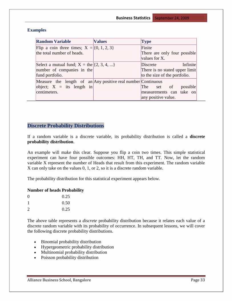
Examples
Random Variable Values Type
Flip a coin three times; X =
the total number of heads.
{0, 1, 2, 3} Finite
There are only four possible
values for X.
Select a mutual fund; X = the
number of companies in the
fund portfolio.
{2, 3, 4, ...} Discrete Infinite
There is no stated upper limit
to the size of the portfolio.
Measure the length of an
object; X = its length in
centimeters.
Any positive real number Continuous
The set of possible
measurements can take on
any positive value.
Discrete Probability Distributions
If a random variable is a discrete variable, its probability distribution is called a discrete
probability distribution.
An example will make this clear. Suppose you flip a coin two times. This simple statistical
experiment can have four possible outcomes: HH, HT, TH, and TT. Now, let the random
variable X represent the number of Heads that result from this experiment. The random variable
X can only take on the values 0, 1, or 2, so it is a discrete random variable.
The probability distribution for this statistical experiment appears below.
Number of heads Probability
0 0.25
1 0.50
2 0.25
The above table represents a discrete probability distribution because it relates each value of a
discrete random variable with its probability of occurrence. In subsequent lessons, we will cover
the following discrete probability distributions.
Binomial probability distribution
Hypergeometric probability distribution
Multinomial probability distribution
Poisson probability distribution

Business Statistics September 24, 2009
Alliance Business School, Bangalore Page 34
Binomial Probability
The binomial probability refers to the probability that a binomial experiment results in
exactly x successes. For example, in the above table, we see that the binomial probability
of getting exactly one head in two coin flips is 0.50.
Given x, n, and P, we can compute the binomial probability based on the following
formula:
Binomial Formula. Suppose a binomial experiment consists of n trials and results in x
successes. If the probability of success on an individual trial is P, then the binomial
probability is:
b(x; n, P) = nCx * Px * (1 - P)
n - x
Example 1
Suppose a die is tossed 5 times. What is the probability of getting exactly 2 fours?
Solution: This is a binomial experiment in which the number of trials is equal to 5, the
number of successes is equal to 2, and the probability of success on a single trial is 1/6 or
about 0.167. Therefore, the binomial probability is:
b(2; 5, 0.167) = 5C2 * (0.167)2 * (0.833)
3
b(2; 5, 0.167) = 0.161
Cumulative Binomial Probability
A cumulative binomial probability refers to the probability that the binomial random variable
falls within a specified range (e.g., is greater than or equal to a stated lower limit and less than or
equal to a stated upper limit).
For example, we might be interested in the cumulative binomial probability of obtaining 45 or
fewer heads in 100 tosses of a coin (see Example 1 below). This would be the sum of all these
individual binomial probabilities.
b(x < 45; 100, 0.5) =
b(x = 0; 100, 0.5) + b(x = 1; 100, 0.5) + ... + b(x = 44; 100, 0.5) + b(x = 45; 100, 0.5)
Business Statistics September 24, 2009
Alliance Business School, Bangalore Page 35
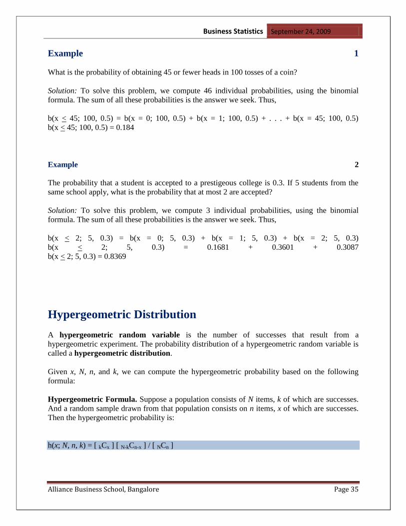
Example 1
What is the probability of obtaining 45 or fewer heads in 100 tosses of a coin?
Solution: To solve this problem, we compute 46 individual probabilities, using the binomial
formula. The sum of all these probabilities is the answer we seek. Thus,
b(x < 45; 100, 0.5) = b(x = 0; 100, 0.5) + b(x = 1; 100, 0.5) + . . . + b(x = 45; 100, 0.5)
b(x < 45; 100, 0.5) = 0.184
Example 2
The probability that a student is accepted to a prestigeous college is 0.3. If 5 students from the
same school apply, what is the probability that at most 2 are accepted?
Solution: To solve this problem, we compute 3 individual probabilities, using the binomial
formula. The sum of all these probabilities is the answer we seek. Thus,
b(x < 2; 5, 0.3) = b(x = 0; 5, 0.3) + b(x = 1; 5, 0.3) + b(x = 2; 5, 0.3)
b(x < 2; 5, 0.3) = 0.1681 + 0.3601 + 0.3087
b(x < 2; 5, 0.3) = 0.8369
Hypergeometric Distribution
A hypergeometric random variable is the number of successes that result from a
hypergeometric experiment. The probability distribution of a hypergeometric random variable is
called a hypergeometric distribution.
Given x, N, n, and k, we can compute the hypergeometric probability based on the following
formula:
Hypergeometric Formula. Suppose a population consists of N items, k of which are successes.
And a random sample drawn from that population consists on n items, x of which are successes.
Then the hypergeometric probability is:
h(x; N, n, k) = [ kCx ] [ N-kCn-x ] / [ NCn ]

Business Statistics September 24, 2009
Alliance Business School, Bangalore Page 36
The hypergeometric distribution has the following properties:
The mean of the distribution is equal to n * k / N .
The variance is n * k * ( N - k ) * ( N - n ) / [ N2 * ( N - 1 ) ] .
Example 1
Suppose we randomly select 5 cards without replacement from an ordinary deck of playing
cards. What is the probability of getting exactly 2 red cards (i.e., hearts or diamonds)?
Solution: This is a hypergeometric experiment in which we know the following:
N = 52; since there are 52 cards in a deck.
k = 26; since there are 26 red cards in a deck.
n = 5; since we randomly select 5 cards from the deck.
x = 2; since 2 of the cards we select are red.
We plug these values into the hypergeometric formula as follows:
h(x; N, n, k) = [ kCx ] [ N-kCn-x ] / [ NCn ]
h(2; 52, 5, 26) = [ 26C2 ] [ 26C3 ] / [ 52C5 ]
h(2; 52, 5, 26) = [ 325 ] [ 2600 ] / [ 2,598,960 ] = 0.32513
Thus, the probability of randomly selecting 2 red cards is 0.32513.
Poisson Distribution
A Poisson random variable is the number of successes that result from a Poisson experiment.
The probability distribution of a Poisson random variable is called a Poisson distribution.
Given the mean number of successes (μ) that occur in a specified region, we can compute the
Poisson probability based on the following formula:
Poisson Formula. Suppose we conduct a Poisson experiment, in which the average number of
successes within a given region is μ. Then, the Poisson probability is:
P(x; μ) = (e-μ
) (μx) / x!
where x is the actual number of successes that result from the experiment, and e is approximately
equal to 2.71828.

Business Statistics September 24, 2009
Alliance Business School, Bangalore Page 37
The Poisson distribution has the following properties:
The mean of the distribution is equal to μ .
The variance is also equal to μ .
Example 1
The average number of homes sold by the Acme Realty company is 2 homes per day. What is
the probability that exactly 3 homes will be sold tomorrow?
Solution: This is a Poisson experiment in which we know the following:
μ = 2; since 2 homes are sold per day, on average.
x = 3; since we want to find the likelihood that 3 homes will be sold tomorrow.
e = 2.71828; since e is a constant equal to approximately 2.71828.
We plug these values into the Poisson formula as follows:
P(x; μ) = (e-μ
) (μx) / x!
P(3; 2) = (2.71828-2
) (23) / 3!
P(3; 2) = (0.13534) (8) / 6
P(3; 2) = 0.180
Thus, the probability of selling 3 homes tomorrow is 0.180 .
Continuous probability distribution
a probability distribution is called continuous if its cumulative distribution function is
continuous, which means that it belongs to a random variable X for which Pr[ X = x ] = 0 for all x
in R.
Another convention reserves the term continuous probability distribution for absolutely
continuous distributions. These distributions can be characterized by a probability density
function: a non-negative Lebesgue integrable function f defined on the real numbers such that
Discrete distributions and some continuous distributions (like the devil's staircase) do not admit
such a density.

Business Statistics September 24, 2009
Alliance Business School, Bangalore Page 38
The Normal Equation
Normal distributions model (some) continuous random variables. Strictly, a Normal random
variable should be capable of assuming any value on the real line, though this requirement is
often waived in practice. For example, height at a given age for a given gender in a given racial
group is adequately described by a Normal random variable even though heights must be
positive.
A continuous random variable X, taking all real values in the range is said to follow a
Normal distribution with parameters µ and if it has probability density function
This probability density function (p.d.f.) is a symmetrical, bell-shaped curve, centred at its
expected value µ. The variance is .
Many distributions arising in practice can be approximated by a Normal distribution. Other
random variables may be transformed to normality.
The simplest case of the normal distribution, known as the Standard Normal Distribution, has
expected value zero and variance one. This is written as N(0,1).
Examples
Example 1
An average light bulb manufactured by the Acme Corporation lasts 300 days with a standard
deviation of 50 days. Assuming that bulb life is normally distributed, what is the probability that
an Acme light bulb will last at most 365 days?

Business Statistics September 24, 2009
Alliance Business School, Bangalore Page 39
Solution: Given a mean score of 300 days and a standard deviation of 50 days, we want to find
the cumulative probability that bulb life is less than or equal to 365 days. Thus, we know the
following:
The value of the normal random variable is 365 days.
The mean is equal to 300 days.
The standard deviation is equal to 50 days.
We enter these values into the Normal Distribution Calculator and compute the cumulative
probability. The answer is: P( X < 365) = 0.90. Hence, there is a 90% chance that a light bulb
will burn out within 365 days.
Uniform Distribution
Uniform distributions model (some) continuous random variables and (some) discrete random
variables. The values of a uniform random variable are uniformly distributed over an interval.
For example, if buses arrive at a given bus stop every 15 minutes, and you arrive at the bus stop
at a random time, the time you wait for the next bus to arrive could be described by a uniform
distribution over the interval from 0 to 15.
A discrete random variable X is said to follow a Uniform distribution with parameters a and b,
written X ~ Un(a,b), if it has probability distribution
P(X=x) = 1/(b-a)
where
x = 1, 2, 3, ......., n.
A discrete uniform distribution has equal probability at each of its n values.
A continuous random variable X is said to follow a Uniform distribution with parameters a and
b, written X ~ Un(a,b), if its probability density function is constant within a finite interval [a,b],
and zero outside this interval (with a less than or equal to b).
The Uniform distribution has expected value E(X)=(a+b)/2 and variance {(b-a)2}/12.
Example

Business Statistics September 24, 2009
Alliance Business School, Bangalore Page 40
SAMPLING AND SAMPLING DISTRIBUTION
Sampling: The process of inferring something about a large group of elements by studying
only a part of it is known as sampling. The collection of all elements about which some reference
is to be made is called the population.
Sampling Distribution: Sampling theory is the study of relationship between a population
and samples drawn from the population, and it is applicable to random sample only. We will
discuss how to estimate the true value of the population parameters (population mean, population
standard deviation and population proportion,…etc) by using sample statistic like sample mean,
sample standard deviation, sample proportion,…etc and to find the limits of accuracy of
estimates based on samples.
The Sampling distribution of a sample statistic calculated from a sample of an
measurements is the probability distribution of a statistic.
Eg : If x has been calculated from a sample of n = 25 measurements selected from a
population with mean µ=0.3 and standard deviation Sigma= 0.005, the sampling
distribution provides information about the behavior (mean) of in repeated sampling.
-if you continue to take samples of data and compute every possible combination of samples (i.e.
all permutations or combinations) of size n then the sample statistics/point estimators can have
their own distribution.
-so each sample statistic/point estimator will have its own distributions with its own mean,
variance, and standard deviation.
-we we know what type of distribution this is we can make probability statements from it and
assess how close the point estimates are to the population parameters (i.e. how close _
x is to μ)
1. Sampling Distribution – the probability distribution of any particular sampling statistic.
2. Law of Large Numbers – if we draw observations from a population with a finite mean
μ at random, as we increase the number of observations we draw the value of the sample mean (_
x ) gets closer and closer to the population mean.

Business Statistics September 24, 2009
Alliance Business School, Bangalore Page 41
-note that this makes sense b/c as you increase the size of your sample it gets closer to the size of
the population. So it begins to look more and more like the population itself. For this reason the
mean should approach the population mean.
3. Sampling Distribution of _
x - this is the probability distribution of all possible values of
a sample mean given a certain size sample n.
Ex:
-Suppose we have a distribution as follows:
If we want to create a sampling distribution we
would take samples of size n, let‘s say 15
from the distribution to the right and from
each sample obtain a mean, variance,
and standard deviation.
…..continue with process for all possible samples of size 15. If we do this we can take the
values from each sample and create its own distribution as shown below.
Graphically:
-notice now we have a distribution of sample means.
This distribution is created from the means of each
sample and it has its own variance and standard
deviation. Note that they should be much
smaller than the distribution sampled from since we created it from the sample means of the data.
x
15 20 25
Sample 2-
has own_
x
, s2, & s
Sample1-
has own_
x
, s2, & s
_
x
20

Business Statistics September 24, 2009
Alliance Business School, Bangalore Page 42
4. Characteristics of the Sampling Distribution of _
x
a. E (_
x ) = μ so the mean of all values of _
x should be the population mean μ
b. Standard Deviation of _
x - called the standard error of the mean it tells us how close our
estimates of the mean are to the actual mean.
i. finite population value – σ _
x = )1/()( NnN * (σ / n )
ii. infinite population - σ _
x = σ / n
note: σ = population variance, N = population size, n = sample size; must still use the infinite
population estimate if n/N < 5% of the population size.
Notice what happens to the distribution of p� as the sample size grows larger…
CENTRAL LIMIT THEOREM
When choosing n and it is a SRS we can assume that the sampling distribution of _
x ~N as N gets
larger and larger. If it is greater than 30 we assume it is Normal.
-if the population is normal, then the sampling distribution must be normal and this rule does not
apply. This is for any size of sample.
-as n increases the variance and standard deviation get tighter and there is a higher probability
that the sample means is within a certain distance of the actual population mean.
Business Statistics September 24, 2009
Alliance Business School, Bangalore Page 43
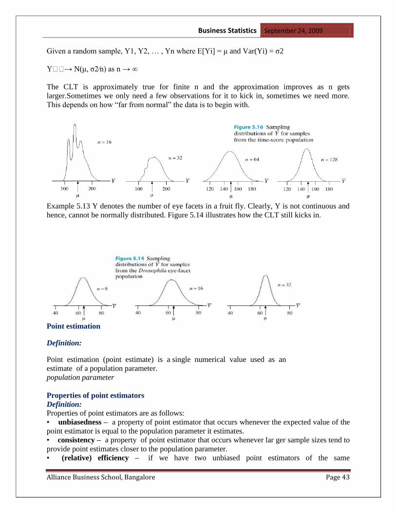
Given a random sample, Y1, Y2, … , Yn where E[Yi] = μ and Var(Yi) = σ2
→ N(μ, σ2⁄n) as n → ∞
The CLT is approximately true for finite n and the approximation improves as n gets
larger.Sometimes we only need a few observations for it to kick in, sometimes we need more.
This depends on how ―far from normal‖ the data is to begin with.
Example 5.13 Y denotes the number of eye facets in a fruit fly. Clearly, Y is not continuous and
hence, cannot be normally distributed. Figure 5.14 illustrates how the CLT still kicks in.
Point estimation
Definition:
Point estimation (point estimate) is a single numerical value used as an
estimate of a population parameter.
population parameter
Properties of point estimators
Definition: Properties of point estimators are as follows:
• unbiasedness – a property of point estimator that occurs whenever the expected value of the
point estimator is equal to the population parameter it estimates.
• consistency – a property of point estimator that occurs whenever lar ger sample sizes tend to
provide point estimates closer to the population parameter.
• (relative) efficiency – if we have two unbiased point estimators of the same

Business Statistics September 24, 2009
Alliance Business School, Bangalore Page 44
population parameter, the point estimator with the smaller variance is said to have gr eater
efficiency than the other.
Usually, we do not know the population mean and standard deviation. Our goal is to estimate
these numbers. The standard way to accomplish this is to use the sample mean and standard
deviation as a best guess for the true population mean and standard deviation. We call this "best
guess" a point estimate.
A Point Estimate is a statistic that gives a plausible estimate for the value in question.
Example:
x is a point estimate for
s is a point estimate for
A point estimate is unbiased if its mean represents the value that it is estimating.
Interval Estimates: An interval estimator (or confidence interval) is a formula that tells us how
to use sample data to calculate an interval that estimates a population parameter. An alternative is
that a certain interval contains the true mean.
Interval Estimates Example: Plugging in the values, the confidence interval is
72.34< <77.66 is the 95% confidence interval for
So there is a 95% probability that this interval contains the true mean
Confidence Intervals
We are not only interested in finding the point estimate for the mean, but also determining how
accurate the point estimate is. The Central Limit Theorem plays a key role here. We assume
that the sample standard deviation is close to the population standard deviation (which will
almost always be true for large samples). Then the Central Limit Theorem tells us that the
standard deviation of the sampling distribution is
2.66)(752.66)-(75
.95)16
2.131(5)X
16
2.131(5)-X( P

Business Statistics September 24, 2009
Alliance Business School, Bangalore Page 45
We will be interested in finding an interval around x such that there is a large probability that the
actual mean falls inside of this interval. This interval is called a confidence interval and the large
probability is called the confidence level.
Example
Suppose that we check for clarity in 50 locations in Lake Tahoe and discover that the average
depth of clarity of the lake is 14 feet. Suppose that we know that the standard deviation for the
entire lake's depth is 2 feet. What can we conclude about the average clarity of the lake with a
95% confidence level?
Solution
We can use x to provide a point estimate for . How accurate is x as a point estimate? We
construct a 95% confidence interval for as follows. We draw the picture and realize that we
need to use the table to find the z-score associated to the probability of .025 (there is .025 to the
left and .025 to the right).
We arrive at z = -1.96. Now we solve for x:
x - 14 x - 14
-1.96 = =
2/ 0.28
Hence
x - 14 = -0.55
We say that 0.55 is the margin of error.
We have that a 95% confidence interval for the mean clarity is
(13.45,14.55)
In other words there is a 95% chance that the mean clarity is between 13.45 and 14.55.

Business Statistics September 24, 2009
Alliance Business School, Bangalore Page 46
In general if zc is the z value associated with c% then a c% confidence interval for the mean is
Example
1000 randomly selected Americans were asked if they believed the minimum wage should be
raised. 600 said yes. Construct a 95% confidence interval for the proportion of Americans who
believe that the minimum wage should be raised.
Solution:
We have
p = 600/1000 = .6 zc = 1.96 and n = 1000
We calculate:
Hence we can conclude that between 57 and 63 percent of all Americans agree with the proposal.
In other words, with a margin of error of .03 , 60% agree.
Confidence Interval for a Mean When the Population Standard Deviation is
Unknown
When the population is normal or if the sample size is large, then the sampling distribution will
also be normal, but the use of s to replace is not that accurate. The smaller the sample size the
worse the approximation will be. Hence we can expect that some adjustment will be made based
on the sample size. The adjustment we make is that we do not use the normal curve for this
approximation. Instead, we use the Student t distribution that is based on the sample size. We
proceed as before, but we change the table that we use. This distribution looks like the normal
distribution, but as the sample size decreases it spreads out. For large n it nearly matches the
normal curve. We say that the distribution has n - 1 degrees of freedom.

Business Statistics September 24, 2009
Alliance Business School, Bangalore Page 47
Example
Suppose that we conduct a survey of 19 millionaires to find out what percent of their income the
average millionaire donates to charity. We discover that the mean percent is 15 with a standard
deviation of 5 percent. Find a 95% confidence interval for the mean percent. Assume that the
distribution of all charity percents is approximately normal.
Solution
We use the formula:
(Notice the t instead of the z and s instead of s)
We get
15 tc 5 /
Since n = 19, there are 18 degrees of freedom. Using the table in the back of the book, we have
that
tc = 2.10
Hence the margin of error is
2.10 (5) / = 2.4
We can conclude with 95% confidence that the millionaires donate between
12.6% and 17.4% of their income to charity.

Business Statistics September 24, 2009
Alliance Business School, Bangalore Page 48
Confidence Intervals for Proportions and
Choosing the Sample Size
A Large Sample Confidence Interval for a Population Proportion
Recall that a confidence interval for a population mean is given by
Confidence Interval for a Population Mean
zc s
x
We can make a similar construction for a confidence interval for a population proportion.
Instead of x, we can use p and instead of s, we use , hence, we can write the
confidence interval for a large sample proportion as
Confidence Interval Margin of Error for a Population Proportion
Example
1000 randomly selected Americans were asked if they believed the minimum wage should be
raised. 600 said yes. Construct a 95% confidence interval for the proportion of Americans who
believe that the minimum wage should be raised.

Business Statistics September 24, 2009
Alliance Business School, Bangalore Page 49
Solution:
We have
p = 600/1000 = .6 zc = 1.96 and n = 1000
We calculate:
Hence we can conclude that between 57 and 63 percent of all Americans agree with the proposal.
In other words, with a margin of error of .03 , 60% agree.
Calculating n for Estimating a Mean
Example
Suppose that you were interested in the average number of units that students take at a two year
college to get an AA degree. Suppose you wanted to find a 95% confidence interval with a
margin of error of .5 for knowing = 10. How many people should we ask?
Solution
Solving for n in
Margin of Error = E = zc /
we have
E = zc
zc
=
E
Squaring both sides, we get

Business Statistics September 24, 2009
Alliance Business School, Bangalore Page 50
We use the formula:
Example
A Subaru dealer wants to find out the age of their customers (for advertising purposes). They
want the margin of error to be 3 years old. If they want a 90% confidence interval, how many
people do they need to know about?
Solution:
We have
E = 3, zc = 1.65
but there is no way of finding sigma exactly. They use the following reasoning: most car
customers are between 16 and 68 years old hence the range is
Range = 68 - 16 = 52
The range covers about four standard deviations hence one standard deviation is about
52/4 = 13
We can now calculate n:
Hence the dealer should survey at least 52 people.

Business Statistics September 24, 2009
Alliance Business School, Bangalore Page 51
Finding n to Estimate a Proportion
Example
Suppose that you are in charge to see if dropping a computer will damage it. You want to find
the proportion of computers that break. If you want a 90% confidence interval for this
proportion, with a margin of error of 4%, How many computers should you drop?
Solution
The formula states that
Squaring both sides, we get that
zc2
p(1 - p)
E2 =
n
Multiplying by n, we get
nE2 = zc
2[p(1 - p)]
This is the formula for finding n.
Since we do not know p, we use .5 ( A conservative estimate)
We round 425.4 up for greater accuracy
We will need to drop at least 426 computers. This could get expensive.

Business Statistics September 24, 2009
Alliance Business School, Bangalore Page 52
Probability Sampling
A probability sample is one in which each member of the population has an equal chance of
being selected - there are four main types of probability sample. The decision as to which
sample to use is dependent upon the nature of the research aim, the desired level of accuracy in
the sample and the availability of a good sampling frame, money and time.
1. Simple Random Sampling
2. Systematic Sampling
3. Stratified Sampling
4. Cluster Sampling
1) Simple Random Sampling
Put simply, this method is where we select a group of people for a study from a larger group i.e.
from a population. Each individual is chosen randomly by chance, and therefore each person has
the same chance as any other of being selected. The easiest way of selecting a sample using this
method is to first obtain a complete sampling frame. Once this has been achieved, each person
within the frame should be allocated a unique reference number starting at one. The size of the
sample must be decided and then that many numbers should be selected, from the table of
random numbers. If the sampling frame consists of 500 people, three digit numbers must be
selected from the random number table, similarly if the highest identifying number on the
sampling frame is a two digit number e.g. 50 you must select two digit numbers from the random
number table. If, as in the example below, the numbers are five digits, simply decide on any two
digits (e.g. first two or last two) and stick to this for the rest of the procedure.
Example
Random Numbers;
Select numbers from every third column and every row. If a number
comes up twice or is larger than the population number, discard it.
Be sure to stick to the pattern of movement through the table.
87456 34098 88900 11128
87456 34098 88900 64554
45666 77789 82276 12555
22333 45767 87900 99989
2) Systematic Sampling
Systematic sampling is very similar to simple random sampling, except instead of selecting
random numbers from tables, you move through the sample frame picking every nth name.

Business Statistics September 24, 2009
Alliance Business School, Bangalore Page 53
In order to do this, it is necessary to work out the sampling fraction. This is done by dividing the
population by the desired sample.
Example
For a population of 100,000 and a desired sample of 2,000, the sampling fraction is 2/100 or
1/50. This means that you would select one person out of every fifty in the population. With
this method, with the sampling fraction of 1/50, the starting point must be within the first 50
people in your list.
This method does bring about a problem worth highlighting. If you used a sampling frame
which is arranged by gender or marital status, problems could occur i.e. if the list was arranged;
Husband/Wife/Husband/Wife etc. and if every tenth person was to be interviewed, there would
be an increased chance of males being selected. This is known as periodicity – if this exists in
the frame it is necessary to either mix up the cases or use Simple Random Sampling.
3) Stratified Sampling
Stratified sampling is a modification of Simple Random Sampling and Systematic Sampling and
is designed to produce a more representative and thus more accurate sample. A stratified sample
is obtained by taking samples from each sub-group of a population. These could be, for
example, age, gender or marital status. The rationale here is to choose 'stratification variables'
that have a major influence on the survey results.
For example, in a lifestyle survey 'age' is likely to have a key effect on 'lifestyle' and you might
want to ensure your sample contains the correct proportion of residents from each age group.
Remember, stratification in this way will only be possible when selecting the sample if the (in
this case) age of the resident is known on the sampling frame.
Having selected the variable, such as age or gender, you need to order the sampling frames into
groups according to the category, and then use systematic sampling to select the appropriate
proportion of people within each variable.
4) Cluster Sampling
This technique is perhaps the most economical of those looked at so far, particularly if face-to-
face interviewing is to be used. As its name suggests, it is a combination of several different
samples. The entire population is divided into groups, or clusters and a random sample of these
clusters are selected. Following that, smaller 'clusters' are chosen from within the selected
clusters.
Multistage cluster sampling is often used when a random sample would produce a list of subjects
so widely scattered geographically that surveying them would prove to be far too expensive. It
should, however, be noted that sampling errors are larger when using cluster sampling.

Business Statistics September 24, 2009
Alliance Business School, Bangalore Page 54
Example
Stage 1: Define population - (say) adults 16+ living in the South East of England.
Stage 2: Select (say) 100 electoral wards from the SE at random
Stage 3: Select a member of smaller areas (e.g. EDS) from within each selected ward.
Stage 4: Interview all residents within the smaller areas (alternatively, select a sample
from the each smaller area.
Non-Probability Sampling
For quantitative surveys, probability sampling should be our preferred approach where possible.
It allows randomness to drive the selection and allows estimates of the accuracy of survey
findings to be obtained. The most likely situation for non-probability sampling to be needed is
when there is either no sampling frame or the population is so widely dispersed that cluster
sampling would be too inefficient. Non-probability techniques are cheaper than probability
sampling, and are often used in exploratory studies e.g. for hypothesis generation. There are five
main non-probability sampling techniques;
1. Purposive Sampling
2. Quota Sampling
3. Convenience Sampling
4. Snowball Sampling
5. Self-Selection
1) Purposive Sampling
Purposive sampling is a method where the participants are selected by the researcher
subjectively. The researcher will pick a sample that he/she believes is representative to the
population of interest. Respondents are not selected randomly but by using the judgment of the
interviewers.
2) Quota Sampling
Quota Sampling is perhaps most commonly used in face-to-face interviewing. Interviewers on
the street are usually looking for a specific type of respondent – age, gender are the most
frequently used 'quota controls'. Quotas are given to interviewers and are organized so that the
final sample is representative of the population. It is impossible to estimate the accuracy of the
sample because it is not random.
3) Convenience Sampling
Similar to quota sampling, convenience sampling is a technique often used in face-to-face
interviewing. A convenience sample is when the interviewer simply stops anyone in the street or
knock on doors asking anyone to participate and interviewing anyone willing to help. It is hard
to draw any meaningful conclusions from the results obtained due to the lack of randomness,
meaning the likelihood of bias is high.

Business Statistics September 24, 2009
Alliance Business School, Bangalore Page 55
4) Snowball Sampling
This approach is often used when trying to interview hard to reach groups such as unemployed
people or Black or Minority Ethnic residents.. You initially contact a few potential respondents,
interview them and then ask if they know of anybody else with the same characteristics you are
looking for.
5) Self-Selection
This technique is self-explanatory – respondents themselves decide whether to take part in the
survey or not.
INFERENCES BASED ON A SINGLE SAMPLE :TESTS
OF HYPOTHESIS
Hypothesis Test
Setting up and testing hypotheses is an essential part of statistical inference. In order to formulate
such a test, usually some theory has been put forward, either because it is believed to be true or
because it is to be used as a basis for argument, but has not been proved, for example, claiming
that a new drug is better than the current drug for treatment of the same symptoms.
In each problem considered, the question of interest is simplified into two competing claims /
hypotheses between which we have a choice; the null hypothesis, denoted H0, against the
alternative hypothesis, denoted H1. These two competing claims / hypotheses are not however
treated on an equal basis: special consideration is given to the null hypothesis.
We have two common situations:
1. The experiment has been carried out in an attempt to disprove or reject a particular
hypothesis, the null hypothesis, thus we give that one priority so it cannot be rejected
unless the evidence against it is sufficiently strong. For example,
H0: there is no difference in taste between coke and diet coke against
H1: there is a difference.
2. If one of the two hypotheses is 'simpler' we give it priority so that a more 'complicated'
theory is not adopted unless there is sufficient evidence against the simpler one. For
example, it is 'simpler' to claim that there is no difference in flavour between coke and
diet coke than it is to say that there is a difference.

Business Statistics September 24, 2009
Alliance Business School, Bangalore Page 56
The hypotheses are often statements about population parameters like expected value and
variance; for example H0 might be that the expected value of the height of ten year old boys in
the Scottish population is not different from that of ten year old girls. A hypothesis might also be
a statement about the distributional form of a characteristic of interest, for example that the
height of ten year old boys is normally distributed within the Scottish population.
The outcome of a hypothesis test test is "Reject H0 in favour of H1" or "Do not reject H0".
Null Hypothesis
The null hypothesis, H0, represents a theory that has been put forward, either because it is
believed to be true or because it is to be used as a basis for argument, but has not been proved.
For example, in a clinical trial of a new drug, the null hypothesis might be that the new drug is
no better, on average, than the current drug. We would write
H0: there is no difference between the two drugs on average.
We give special consideration to the null hypothesis. This is due to the fact that the null
hypothesis relates to the statement being tested, whereas the alternative hypothesis relates to the
statement to be accepted if / when the null is rejected.
The final conclusion once the test has been carried out is always given in terms of the null
hypothesis. We either "Reject H0 in favour of H1" or "Do not reject H0"; we never conclude
"Reject H1", or even "Accept H1".
If we conclude "Do not reject H0", this does not necessarily mean that the null hypothesis is true,
it only suggests that there is not sufficient evidence against H0 in favor of H1. Rejecting the null
hypothesis then, suggests that the alternative hypothesis may be true.
Alternative Hypothesis
The alternative hypothesis, H1, is a statement of what a statistical hypothesis test is set up to
establish. For example, in a clinical trial of a new drug, the alternative hypothesis might be that
the new drug has a different effect, on average, compared to that of the current drug. We would
write
H1: the two drugs have different effects, on average.
The alternative hypothesis might also be that the new drug is better, on average, than the current
drug. In this case we would write
H1: the new drug is better than the current drug, on average.

Business Statistics September 24, 2009
Alliance Business School, Bangalore Page 57
The final conclusion once the test has been carried out is always given in terms of the null
hypothesis. We either "Reject H0 in favour of H1" or "Do not reject H0". We never conclude
"Reject H1", or even "Accept H1".
If we conclude "Do not reject H0", this does not necessarily mean that the null hypothesis is true,
it only suggests that there is not sufficient evidence against H0 in favor of H1. Rejecting the null
hypothesis then, suggests that the alternative hypothesis may be true.
Simple Hypothesis
A simple hypothesis is a hypothesis which specifies the population distribution completely.
Examples
1. H0: X ~ Bi(100,1/2), i.e. p is specified
2. H0: X ~ N(5,20), i.e. µ and are specified
Composite Hypothesis
A composite hypothesis is a hypothesis which does not specify the population distribution
completely.
Examples
1. X ~ Bi(100,p) and H1: p > 0.5
2. X ~ N(0, ) and H1: unspecified
Type I Error
In a hypothesis test, a type I error occurs when the null hypothesis is rejected when it is in fact
true; that is, H0 is wrongly rejected.
For example, in a clinical trial of a new drug, the null hypothesis might be that the new drug is
no better, on average, than the current drug; i.e.
H0: there is no difference between the two drugs on average.
A type I error would occur if we concluded that the two drugs produced different effects when in
fact there was no difference between them.

Business Statistics September 24, 2009
Alliance Business School, Bangalore Page 58
The following table gives a summary of possible results of any hypothesis test:
Decision
Reject H0 Don't reject H0
Truth
H0 Type I Error Right decision
H1 Right decision Type II Error
A type I error is often considered to be more serious, and therefore more important to avoid, than
a type II error. The hypothesis test procedure is therefore adjusted so that there is a guaranteed
'low' probability of rejecting the null hypothesis wrongly; this probability is never 0. This
probability of a type I error can be precisely computed as
P(type I error) = significance level =
The exact probability of a type II error is generally unknown.
If we do not reject the null hypothesis, it may still be false (a type II error) as the sample may not
be big enough to identify the falseness of the null hypothesis (especially if the truth is very close
to hypothesis).
For any given set of data, type I and type II errors are inversely related; the smaller the risk of
one, the higher the risk of the other.
A type I error can also be referred to as an error of the first kind.
Type II Error
In a hypothesis test, a type II error occurs when the null hypothesis H0, is not rejected when it is
in fact false. For example, in a clinical trial of a new drug, the null hypothesis might be that the
new drug is no better, on average, than the current drug; i.e.
H0: there is no difference between the two drugs on average.
A type II error would occur if it was concluded that the two drugs produced the same effect, i.e.
there is no difference between the two drugs on average, when in fact they produced different
ones.

Business Statistics September 24, 2009
Alliance Business School, Bangalore Page 59
A type II error is frequently due to sample sizes being too small.
The probability of a type II error is generally unknown, but is symbolized by and written
P(type II error) =
A type II error can also be referred to as an error of the second kind.
Test Statistic
A test statistic is a quantity calculated from our sample of data. Its value is used to decide
whether or not the null hypothesis should be rejected in our hypothesis test.
The choice of a test statistic will depend on the assumed probability model and the hypotheses
under question.
Critical Value(s)
The critical value(s) for a hypothesis test is a threshold to which the value of the test statistic in a
sample is compared to determine whether or not the null hypothesis is rejected.
The critical value for any hypothesis test depends on the significance level at which the test is
carried out, and whether the test is one-sided or two-sided.
Critical Region
The critical region CR, or rejection region RR, is a set of values of the test statistic for which the
null hypothesis is rejected in a hypothesis test. That is, the sample space for the test statistic is
partitioned into two regions; one region (the critical region) will lead us to reject the null
hypothesis H0, the other will not. So, if the observed value of the test statistic is a member of the
critical region, we conclude "Reject H0"; if it is not a member of the critical region then we
conclude "Do not reject H0".

Business Statistics September 24, 2009
Alliance Business School, Bangalore Page 60
Significance Level
The significance level of a statistical hypothesis test is a fixed probability of wrongly rejecting
the null hypothesis H0, if it is in fact true.
It is the probability of a type I error and is set by the investigator in relation to the consequences
of such an error. That is, we want to make the significance level as small as possible in order to
protect the null hypothesis and to prevent, as far as possible, the investigator from inadvertently
making false claims.
The significance level is usually denoted by
Significance Level = P(type I error) =
Usually, the significance level is chosen to be 0.05 (or equivalently, 5%).
P-Value
The probability value (p-value) of a statistical hypothesis test is the probability of getting a value
of the test statistic as extreme as or more extreme than that observed by chance alone, if the null
hypothesis H0, is true.
It is the probability of wrongly rejecting the null hypothesis if it is in fact true.
It is equal to the significance level of the test for which we would only just reject the null
hypothesis. The p-value is compared with the actual significance level of our test and, if it is
smaller, the result is significant. That is, if the null hypothesis were to be rejected at the 5%
significance level, this would be reported as "p < 0.05".
Small p-values suggest that the null hypothesis is unlikely to be true. The smaller it is, the more
convincing is the rejection of the null hypothesis. It indicates the strength of evidence for say,
rejecting the null hypothesis H0, rather than simply concluding "Reject H0' or "Do not reject
H0".
Power
The power of a statistical hypothesis test measures the test's ability to reject the null hypothesis
when it is actually false - that is, to make a correct decision.
In other words, the power of a hypothesis test is the probability of not committing a type II error.
It is calculated by subtracting the probability of a type II error from 1, usually expressed as:
Power = 1 - P(type II error) =

Business Statistics September 24, 2009
Alliance Business School, Bangalore Page 61
The maximum power a test can have is 1, the minimum is 0. Ideally we want a test to have high
power, close to 1.
One-sided Test
A one-sided test is a statistical hypothesis test in which the values for which we can reject the
null hypothesis, H0 are located entirely in one tail of the probability distribution.
In other words, the critical region for a one-sided test is the set of values less than the critical
value of the test, or the set of values greater than the critical value of the test.
A one-sided test is also referred to as a one-tailed test of significance.
The choice between a one-sided and a two-sided test is determined by the purpose of the
investigation or prior reasons for using a one-sided test.
Example
Suppose we wanted to test a manufacturer‘s claim that there are, on average, 50 matches in a
box. We could set up the following hypotheses
H0: µ = 50, against
H1: µ < 50 or H1: µ > 50
Either of these two alternative hypotheses would lead to a one-sided test. Presumably, we would
want to test the null hypothesis against the first alternative hypothesis since it would be useful to
know if there is likely to be less than 50 matches, on average, in a box (no one would complain if
they get the correct number of matches in a box or more).
Yet another alternative hypothesis could be tested against the same null, leading this time to a
two-sided test:
H0: µ = 50, against
H1: µ not equal to 50
Here, nothing specific can be said about the average number of matches in a box; only that, if we
could reject the null hypothesis in our test, we would know that the average number of matches
in a box is likely to be less than or greater than 50.

Business Statistics September 24, 2009
Alliance Business School, Bangalore Page 62
Two-Sided Test
A two-sided test is a statistical hypothesis test in which the values for which we can reject the
null hypothesis, H0 are located in both tails of the probability distribution.
In other words, the critical region for a two-sided test is the set of values less than a first critical
value of the test and the set of values greater than a second critical value of the test.
A two-sided test is also referred to as a two-tailed test of significance.
The choice between a one-sided test and a two-sided test is determined by the purpose of the
investigation or prior reasons for using a one-sided test.
Example
Suppose we wanted to test a manufacturer‘s claim that there are, on average, 50 matches in a
box. We could set up the following hypotheses
H0: µ = 50, against
H1: µ < 50 or H1: µ > 50
Either of these two alternative hypotheses would lead to a one-sided test. Presumably, we would
want to test the null hypothesis against the first alternative hypothesis since it would be useful to
know if there is likely to be less than 50 matches, on average, in a box (no one would complain if
they get the correct number of matches in a box or more).
Yet another alternative hypothesis could be tested against the same null, leading this time to a
two-sided test:
H0: µ = 50, against
H1: µ not equal to 50
Here, nothing specific can be said about the average number of matches in a box; only that, if we
could reject the null hypothesis in our test, we would know that the average number of matches
in a box is likely to be less than or greater than 50.

Business Statistics September 24, 2009
Alliance Business School, Bangalore Page 63
T-TEST
The t-test assesses whether the means of two groups are statistically different from each other.
This analysis is appropriate whenever you want to compare the means of two groups.
Example: Sam hypothesizes that people who are allowed to sleep for only four hours will score
significantly lower than people who are allowed to sleep for eight hours on a cognitive skills test.
He brings sixteen participants into his sleep lab and randomly assigns them to one of two groups.
In one group he has participants sleep for eight hours and in the other group he has them sleep
for four. The next morning he administers the SCAT (Sam's Cognitive Ability Test) to all
participants. (Scores on the SCAT range from 1-9 with high scores representing better
performance).
SCAT scores
8 hours sleep
group (X) 5 7 5 3 5 3 3 9
4 hours sleep
group (Y) 8 1 4 6 6 4 1 2
X (x-Mx)2 y (y - My)
2
5 0 8 16
7 4 1 9
5 0 4 0
3 4 6 4
5 0 5 4
3 4 4 0
3 4 1 9
9 16 2 4
x=40 (x-
Mx)2=32
y=32 (y-
My)2=46
Mx=5
My=4

Business Statistics September 24, 2009
Alliance Business School, Bangalore Page 64
Interpretation: Sam's hypothesis was not confirmed. He did not find a significant difference
between those who slept for four hours versus those who slept for eight hours on cognitive test
performance.
One Sample t-test
A one sample t-test is a hypothesis test for answering questions about the mean where the data
are a random sample of independent observations from an underlying normal distribution N(µ,
), where is unknown.
The null hypothesis for the one sample t-test is:
H0: µ = µ0, where µ0 is known.
That is, the sample has been drawn from a population of given mean and unknown variance
(which therefore has to be estimated from the sample).
This null hypothesis, H0 is tested against one of the following alternative hypotheses, depending
on the question posed:
H1: µ is not equal to µ
H1: µ > µ
H1: µ < µ

Business Statistics September 24, 2009
Alliance Business School, Bangalore Page 65
Two Sample t-test
A two sample t-test is a hypothesis test for answering questions about the mean where the data
are collected from two random samples of independent observations, each from an underlying
normal distribution:
When carrying out a two sample t-test, it is usual to assume that the variances for the two
populations are equal, i.e.
The null hypothesis for the two sample t-test is:
H0: µ1 = µ2
That is, the two samples have both been drawn from the same population. This null hypothesis is
tested against one of the following alternative hypotheses, depending on the question posed.
H1: µ1 is not equal to µ2
H1: µ1 > µ2
H1: µ1 < µ2
Z Test
Description
The Z-test compares sample and population means to determine if there is a significant
difference.
It requires a simple random sample from a population with a Normal distribution and where
the mean is known.
Calculation
The z measure is calculated as:
z = (x - ) / SE
where x is the mean sample to be standardized, (mu) is the population mean and
SE is the standard error of the mean.
SE = / SQRT(n)

Business Statistics September 24, 2009
Alliance Business School, Bangalore Page 66
where is the population standard deviation and n is the sample size.
The z value is then looked up in a z-table. A negative z value means it is below the population
mean (the sign is ignored in the lookup table).
Discussion
The Z-test is typically with standardized tests, checking whether the scores from a particular
sample are within or outside the standard test performance.
The z value indicates the number of standard deviation units of the sample from the population
mean.
Comparing a Population Proportion to a Sample Proportion (Z-test)
Used to compare a proportion created by a random sample to a proportion originating from or
thought to represent the value for the entire population. As an example, to make sure your
random sample of 100 subjects is not biased regarding a person‘s sex, you could compare the
proportion of women in the sample to the known proportion of women in the underlying
population as reported in census data or by some other reliable source.
Example: Historical data indicates that about 10% of your agency's clients believe they were
given poor service. Now under new management for six months, a random sample of 110 clients
found that 15% believe they were given poor service.
Pu = .10
Ps = .15
n = 110
Assumptions
Independent random sampling
Nominal level data
Large sample size
State the Hypothesis
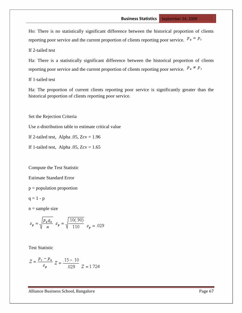
Business Statistics September 24, 2009
Alliance Business School, Bangalore Page 67
Ho: There is no statistically significant difference between the historical proportion of clients
reporting poor service and the current proportion of clients reporting poor service.
If 2-tailed test
Ha: There is a statistically significant difference between the historical proportion of clients
reporting poor service and the current proportion of clients reporting poor service.
If 1-tailed test
Ha: The proportion of current clients reporting poor service is significantly greater than the
historical proportion of clients reporting poor service.
Set the Rejection Criteria
Use z-distribution table to estimate critical value
If 2-tailed test, Alpha .05, Zcv = 1.96
If 1-tailed test, Alpha .05, Zcv = 1.65
Compute the Test Statistic
Estimate Standard Error
p = population proportion
q = 1 - p
n = sample size
Test Statistic

Business Statistics September 24, 2009
Alliance Business School, Bangalore Page 68
Decide Results of Null Hypothesis
If a 2-tailed test was used
Since the test statistic of 1.724 did not meet or exceed the critical value of 1.96, there is
insufficient evidence to conclude there is a statistically significant difference between the
historical proportion of clients reporting poor service and the current proportion of clients
reporting poor service.
If a 1-tailed test was used
Since the test statistic of 1.724 exceeds the critical value of 1.65, you can conclude the
proportion of current clients reporting poor service is significantly greater than the historical
proportion of clients reporting poor service.
Comparing Proportions From Two Independent Samples
(Z-test)
Used to compare two proportions created by two random samples or two subgroups of one
random sample.
EXAMPLE: A survey was conducted of students from the Princeton public school system to
determine if the incidence of hungry children was consistent in two schools located in lower-
income areas. A random sample of 80 elementary students from school A found that 23% did not
have breakfast before coming to school. A random sample of 180 elementary students from
school B found that 7% did not have breakfast before coming to school.
Assumptions
Independent random sampling
Nominal level data
Large sample size

Business Statistics September 24, 2009
Alliance Business School, Bangalore Page 69
State the Hypothesis
Ho: There is no statistically significant difference between the proportion of students in
school A not eating breakfast and the proportion of students in school B not eating
breakfast.
Ha: There is a statistically significant difference between the proportion of students in
school A not eating breakfast and the proportion of students in school B not eating
breakfast.
Set the Rejection Criteria
Use z-distribution table to estimate critical value
Alpha.05, Zcv = 1.96
Compute the Test Statistic
Estimate of Standard Error
where and
Test Statistic

Business Statistics September 24, 2009
Alliance Business School, Bangalore Page 70
Decide Results of the Null Hypothesis
Since the test statistic 3.721 exceeds the critical value of 1.96, you conclude there is a
statistically significant difference between the proportion of students in school A not
eating breakfast and the proportion of students in school B not eating breakfast.
The F-distribution is formed by the ratio of two independent chi-square variables divided by their
respective degrees of freedom.
Since F is formed by chi-square, many of the chi-square properties carry over to the F
distribution.
The F-values are all non-negative
The distribution is non-symmetric
The mean is approximately 1
There are two independent degrees of freedom, one for the numerator, and one for the
denominator.
There are many different F distributions, one for each pair of degrees of freedom.
F-Test
The F-test is designed to test if two population variances are equal. It does this by comparing the
ratio of two variances. So, if the variances are equal, the ratio of the variances will be 1.
If the null hypothesis is true, then the F test-statistic given above can be simplified
(dramatically). This ratio of sample variances will be test statistic used. If the null hypothesis is

Business Statistics September 24, 2009
Alliance Business School, Bangalore Page 71
false, then we will reject the null hypothesis that the ratio was equal to 1 and our assumption that
they were equal.
There are several different F-tables. Each one has a different level of significance. So, find the
correct level of significance first, and then look up the numerator degrees of freedom and the
denominator degrees of freedom to find the critical value.
You will notice that all of the tables only give level of significance for right tail tests. Because
the F distribution is not symmetric, and there are no negative values, you may not simply take
the opposite of the right critical value to find the left critical value. The way to find a left critical
value is to reverse the degrees of freedom, look up the right critical value, and then take the
reciprocal of this value. For example, the critical value with 0.05 on the left with 12 numerator
and 15 denominator degrees of freedom is found of taking the reciprocal of the critical value
with 0.05 on the right with 15 numerator and 12 denominator degrees of freedom.
Assumptions / Notes
The larger variance should always be placed in the numerator
The test statistic is F = s1^2 / s2^2 where s1^2 > s2^2
Divide alpha by 2 for a two tail test and then find the right critical value
If standard deviations are given instead of variances, they must be squared
When the degrees of freedom aren't given in the table, go with the value with the larger
critical value (this happens to be the smaller degrees of freedom). This is so that you are
less likely to reject in error (type I error)
The populations from which the samples were obtained must be normal.
The samples must be independent
EXAMPLE:
If we are not interested in whether one method is better compared to another, but were simply
trying to determine if the variances of were the same or different, we would need to use a 2-
tailed test. For instance, assume we made two sets of measurements of ethanol concentration in a
sample of vodka using the same instrument, but on two different days. On the first day, we found
a standard deviation of s1 = 9 ppm and on the next day we found s2 = 2 ppm. Both datasets
comprised 6 measurements. We want to know if we can combine the two datasets, or if there is a
significant difference between the datasets, and that we should discard one of them.
As usual, we begin by defining the null hypothesis, H0: σ12 = σ2
2, and the alternate hypothesis,
HA: σ12 ≠ σ2
2. The "≠" sign indicates that this is a 2-tailed test, because we are interested in both
cases: σ12 > σ2
2 and σ1
2 < σ2
2. For the F-test, you can perform a 2-tailed test by multiplying the

Business Statistics September 24, 2009
Alliance Business School, Bangalore Page 72
confidence level P by 2, so from a table for a 1-tailed test at the P = 0.05 confidence level, we
would perform a 2-tailed test at P = 0.10, or a 90% confidence level.
For this dataset, s2 > s1, Fcalc = s12/ s2
2 = 9
2/2
2 = 20.25. The tabulated value for ν = 5 at 90%
confidence is F5,5 = 5.050. Since Fcalc > F5,5, we reject the null hypothesis, and can say with 90%
certainty that there is a difference between the standard deviations of the two methods.
Tables for other confidence levels can be found in most statistics or analytical chemistry
textbooks. Be careful when using these tables, to pay attention to whether the table is for a 1- or
a 2-tailed test. In most cases, tables are given for 2-tailed tests, so you can divide by 2 for the 1-
tailed test. For the F-test, always ensure that the larger standard deviation is in the numerator, so
that F ≥ 1.
EXAMPLE 2:
In this example we test the equality of the variances of two data sets that belong to a normal
distribution. We start this example by creating 3 waves of different statistics. The first pair (data1
and data2) have the same variance but different means. The second pair (data2 and data3) have
the same mean but different variance. To create the data execute the commands:
Make/n=100 data1=100+gnoise(3)
Make/n=80 data2=80+gnoise(3)
Make/N=90 data3=80+gnoise(4)
Comparing the variance of two waves using a two-tailed hypothesis
To run the test execute the command:
StatsFTest/T=1/Q data1,data2
The results of the test appear in the F-Test table:
n1 100
Mean1 99.8754
Stdv1 3.39174
degreesOfFreedom1 99
n2 80
Mean2 79.6029
Stdv2 3.10709
degreesOfFreedom2 79
F 1.19162
lowCriticalValue 0.659763
highCriticalValue 1.53104

Business Statistics September 24, 2009
Alliance Business School, Bangalore Page 73
P 0.418974
Accept 1
The F statistic is within the critical range so the two-tailed hypothesis of equal variances is
accepted.
Testing in the case of unequal variances (two tails test)
To run the test execute the following command:
StatsFTest/T=1/Q data1,data3
The results of the test appear in the F-Test table:
n1 100
Mean1 99.8754
Stdv1 3.39174
degreesOfFreedom1 99
n2 80
Mean2 80.5489
Stdv2 4.43966
degreesOfFreedom2 79
F 0.583641
lowCriticalValue 0.659763
highCriticalValue 1.53104
P 0.0112429
Accept 0
The rejection of H0 in this case is pretty sensitive to the choice of significance. It is apparent
from the P-value that it would have been accepted if alpha was set to 0.01.
One-tail testing for the same data
First H0: the variance of the first sample is greater than the variance of the second. To run the test
execute the command:
StatsFTest/T=1/Q/TAIL=1 data1,data3
n1 100
Mean1 99.8754
Stdv1 3.39174
degreesOfFreedom1 99

Business Statistics September 24, 2009
Alliance Business School, Bangalore Page 74
n2 80
Mean2 80.5489
Stdv2 4.43966
degreesOfFreedom2 79
F 0.583641
Critical 0.70553
P 0.00562143
Accept 0
H0 is rejected here as one would expect. Similarly,
StatsFTest/T=1/Q/TAIL=2 data1,data3
n1 100
Mean1 99.8754
Stdv1 3.39174
degreesOfFreedom1 99
n2 80
Mean2 80.5489
Stdv2 4.43966
degreesOfFreedom2 79
F 0.583641
Critical 1.4289
P 0.00562143
Accept 1
Here the F is smaller than the critical value so the two-tailed hypothesis can't be rejected.
Chi-Square Test
Chi-square is a statistical test commonly used to compare observed data with data we would
expect to obtain according to a specific hypothesis. For example, if, according to Mendel's laws,
you expected 10 of 20 offspring from a cross to be male and the actual observed number was 8
males, then you might want to know about the "goodness to fit" between the observed and
expected. Were the deviations (differences between observed and expected) the result of chance,
or were they due to other factors. How much deviation can occur before you, the investigator,
must conclude that something other than chance is at work, causing the observed to differ from
the expected. The chi-square test is always testing what scientists call the null hypothesis, which
states that there is no significant difference between the expected and observed result.

Business Statistics September 24, 2009
Alliance Business School, Bangalore Page 75
The formula for calculating chi-square ( 2) is:
2= (o-e)
2/e
That is, chi-square is the sum of the squared difference between observed (o) and the expected
(e) data (or the deviation, d), divided by the expected data in all possible categories.
For example, suppose that a cross between two pea plants yields a population of 880 plants, 639
with green seeds and 241 with yellow seeds. You are asked to propose the genotypes of the
parents. Your hypothesis is that the allele for green is dominant to the allele for yellow and that
the parent plants were both heterozygous for this trait. If your hypothesis is true, then the
predicted ratio of offspring from this cross would be 3:1 (based on Mendel's laws) as predicted
from the results of the Punnett square (Figure B. 1).
Figure B.1 - Punnett Square. Predicted offspring from cross
between green and yellow-seeded plants. Green (G) is dominant
(3/4 green; 1/4 yellow).
To calculate 2 , first determine the number expected in each category. If the ratio is 3:1 and the
total number of observed individuals is 880, then the expected numerical values should be 660
green and 220 yellow.
Chi-square requires that you use numerical values, not percentages or ratios.
Then calculate 2 using this formula, as shown in Table B.1. Note that we get a value of 2.668
for 2. But what does this number mean? Here's how to interpret the
2 value:
1. Determine degrees of freedom (df). Degrees of freedom can be calculated as the number of
categories in the problem minus 1. In our example, there are two categories (green and yellow);
therefore, there is I degree of freedom.
2. Determine a relative standard to serve as the basis for accepting or rejecting the hypothesis.
The relative standard commonly used in biological research is p > 0.05. The p value is the
probability that the deviation of the observed from that expected is due to chance alone (no other

Business Statistics September 24, 2009
Alliance Business School, Bangalore Page 76
forces acting). In this case, using p > 0.05, you would expect any deviation to be due to chance
alone 5% of the time or less.
3. Refer to a chi-square distribution table (Table B.2). Using the appropriate degrees of 'freedom,
locate the value closest to your calculated chi-square in the table. Determine the closestp
(probability) value associated with your chi-square and degrees of freedom. In this case (2=2.668), the p value is about 0.10, which means that there is a 10% probability that any
deviation from expected results is due to chance only. Based on our standard p > 0.05, this is
within the range of acceptable deviation. In terms of your hypothesis for this example, the
observed chi-squareis not significantly different from expected. The observed numbers are
consistent with those expected under Mendel's law.
Step-by-Step Procedure for Testing Your Hypothesis and Calculating Chi-Square
1. State the hypothesis being tested and the predicted results. Gather the data by conducting the
proper experiment (or, if working genetics problems, use the data provided in the problem).
2. Determine the expected numbers for each observational class. Remember to use numbers, not
percentages.
Chi-square should not be calculated if the expected value in any category is less than 5.
3. Calculate 2 using the formula. Complete all calculations to three significant digits. Round off
your answer to two significant digits.
4. Use the chi-square distribution table to determine significance of the value.
a. Determine degrees of freedom and locate the value in the appropriate column.
b. Locate the value closest to your calculated 2 on that degrees of freedom df row.
c. Move up the column to determine the p value.
5. State your conclusion in terms of your hypothesis.
a. If the p value for the calculated 2 is p > 0.05, accept your hypothesis. 'The deviation is
small enough that chance alone accounts for it. A p value of 0.6, for example, means that
there is a 60% probability that any deviation from expected is due to chance only. This is
within the range of acceptable deviation.
b. If the p value for the calculated 2 is p < 0.05, reject your hypothesis, and conclude that
some factor other than chance is operating for the deviation to be so great. For example, a
p value of 0.01 means that there is only a 1% chance that this deviation is due to chance
alone. Therefore, other factors must be involved.

Business Statistics September 24, 2009
Alliance Business School, Bangalore Page 77
The chi-square test will be used to test for the "goodness to fit" between observed and expected
data from several laboratory investigations in this lab manual.
Table 1
Calculating Chi-Square
Green Yellow
Observed (o) 639 241
Expected (e) 660 220
Deviation (o - e) -21 21
Deviation2 (d2) 441 441
d2/e 0.668 2
2 = d
2/e = 2.668 . .
Table 2 Chi-Square Distribution
Degrees
of
Freedom
(df)
Probability (p)
0.95 0.90 0.80 0.70 0.50 0.30 0.20 0.10 0.05 0.01 0.001
1 0.004 0.02 0.06 0.15 0.46 1.07 1.64 2.71 3.84 6.64 10.83
2 0.10 0.21 0.45 0.71 1.39 2.41 3.22 4.60 5.99 9.21 13.82
3 0.35 0.58 1.01 1.42 2.37 3.66 4.64 6.25 7.82 11.34 16.27
4 0.71 1.06 1.65 2.20 3.36 4.88 5.99 7.78 9.49 13.28 18.47
5 1.14 1.61 2.34 3.00 4.35 6.06 7.29 9.24 11.07 15.09 20.52
6 1.63 2.20 3.07 3.83 5.35 7.23 8.56 10.64 12.59 16.81 22.46
7 2.17 2.83 3.82 4.67 6.35 8.38 9.80 12.02 14.07 18.48 24.32
8 2.73 3.49 4.59 5.53 7.34 9.52 11.03 13.36 15.51 20.09 26.12
9 3.32 4.17 5.38 6.39 8.34 10.66 12.24 14.68 16.92 21.67 27.88
10 3.94 4.86 6.18 7.27 9.34 11.78 13.44 15.99 18.31 23.21 29.59
Nonsignificant Significant

Business Statistics September 24, 2009
Alliance Business School, Bangalore Page 78
COMPARING POPULATION MEANS AND
PROPORTIONS
Sampling Distribution of the Differences between the Two Sample Means for Independent
Samples
When one wants to estimate the difference between two population means from independent
samples, then one will use a t-interval to calculate a confidence interval. If the sample variances
are not very different, one can use the pooled 2-sample t-interval.
Step 1. Find with df = n1 + n2 - 2.
Step 2. The endpoints of the (1 - ) 100% confidence interval for - is:
the degrees of freedom of t are n1 + n2 - 2.
Continuing from the previous example, give a 99% confidence interval for the difference
between the mean time it takes the new machine to pack ten cartons and the mean time it takes
the present machine to pack ten cartons.
Step 1. = 0.01, = t0.005 = 2.878, where the degrees of freedom are 18.
Step 2.
The 99% confidence interval is (-2.01, -0.17).
Interpret the above result:
We are 99% confident that - is between -2.01 and -0.17.

Business Statistics September 24, 2009
Alliance Business School, Bangalore Page 79
Paired samples:
The sample selected from the first population is related to the corresponding sample from the
second population.
When we use paired data we are looking at the difference of μ1 vs. μ2 - we write it μ1 - μ2 = μd. A
helpful chart for determining our hypothesis is:
Hypothesis Paired sample hypothesis p-value
H0: μ1 - μ2 = some hypothesized
value
H0: μd = some hypothesized
value
H0: μ1 - μ2 ≥ some hypothesized
value
Ha: μd > some hypothesized
value
area under the curve to the
right of the calculated t
H0: μ1 - μ2 ≤ some hypothesized
value
Ha: μd < some hypothesized
value
area under the curve to the
left of the calculated t
H0: μ1 - μ2 ≠ some hypothesized
value
Ha: μd ≠ some hypothesized
value
1) 2(area to the right oft) if t
is positive, or
2) 2( area to the left of t) if t
is negative
Trace metals in drinking water affect the flavor and an unusually high concentration can pose a
health hazard. Ten pairs of data were taken measuring zinc concentration in bottom water and
surface water. Does the data suggest that the true average concentration in the bottom water
exceeds that of surface water?
Location
1 2 3 4 5 6 7 8 9 10
Zinc
concentration
in
bottom water
.430 .266 .567 .531 .707 .716 .651 .589 .469 .723
Zinc
concentration
in
surface water
.415 .238 .390 .410 .605 .609 .632 .523 .411 .612

Business Statistics September 24, 2009
Alliance Business School, Bangalore Page 80
Paired t-Procedure:
Assumptions:
1. Paired samples
2. The differences of the pairs follow a normal distribution or the number of pairs is
large (note here that if the number of pairs is < 30, we need to check whether the
differences are normal, but we do not need to check for the normality of each
population)
Hypothesis:
Ho: - = 0
Ha: - 0
OR
Ho: - = 0
Ha: - < 0
OR
Ho: - = 0
Ha: - > 0
t-statistic:
Let = - ,
degrees of freedom = n - 1
where n denotes the number of pairs.
Paired t-interval:

Business Statistics September 24, 2009
Alliance Business School, Bangalore Page 81
An Example for the Paired t-Test
To perform a paired t-test for the previous trace metal example:
Assumptions:
1. Is this a paired sample?
Yes.
2. Is this a large sample?
No.
3. Since the sample size is not large enough (less than 30), we need to check whether the
differences follow a normal distribution.
F-test to compare Two Population Variances
In Lesson 10 I promised to show you how to statistically compare the variances of two
quantitative variables. We use the F-test to do this. When we test the equality of variances the
hypotheses of interest are:
Ho: 12 - 2
2 = 0
Ha: 12 - 2
2 0
An Example to Compare Two Population Variances
We return to the data on packaging time from Lesson 10. We are going to determine if it is
reasonable to assume that the two machines have equal population variances. Recall that the data
are given as:
New Machine Old Machine
42.1 41.3 42.4 43.2 41.8 42.7 43.8 42.5 43.1 44.0
41.0 41.8 42.8 42.3 42.7 43.6 43.3 43.5 41.7 44.1
= 42.14, s1 = 0.683 = 43.23, s2 = 0.750

Business Statistics September 24, 2009
Alliance Business School, Bangalore Page 82
Linear regression
Introduction to linear regression
Linear regression analyzes the relationship between two variables, X and Y. For each subject (or
experimental unit), you know both X and Y and you want to find the best straight line through
the data. In some situations, the slope and/or intercept have a scientific meaning. In other cases,
you use the linear regression line as a standard curve to find new values of X from Y, or Y from
X.
The term "regression", like many statistical terms, is used in statistics quite differently than it is
used in other contexts. The method was first used to examine the relationship between the
heights of fathers and sons. The two were related, of course, but the slope is less than 1.0. A tall
father tended to have sons shorter than himself; a short father tended to have sons taller than
himself. The height of sons regressed to the mean. The term "regression" is now used for many
sorts of curve fitting.
Prism determines and graphs the best-fit linear regression line, optionally including a 95%
confidence interval or 95% prediction interval bands. You may also force the line through a
particular point (usually the origin), calculate residuals, calculate a runs test, or compare the
slopes and intercepts of two or more regression lines.
In general, the goal of linear regression is to find the line that best predicts Y from X. Linear
regression does this by finding the line that minimizes the sum of the squares of the vertical
distances of the points from the line.
Note that linear regression does not test whether your data are linear (except via the runs test). It
assumes that your data are linear, and finds the slope and intercept that make a straight line best
fit your data.
Definitions
a) A scatterplot is a graph of paired X and Y values
b) A linear relationship is one in which the relationship between X and Y can best be
represented by a straight line.
c) A curvilinear relationship is one in which the relationship between X and Y can best be
represented by a curved line.
d) A perfect relationship exists when all of the points in the scatter plot fall exactly on the line
(or curve). An imperfect relationship is one in which there is a relationship, but not all
points fall on the line (or curve).
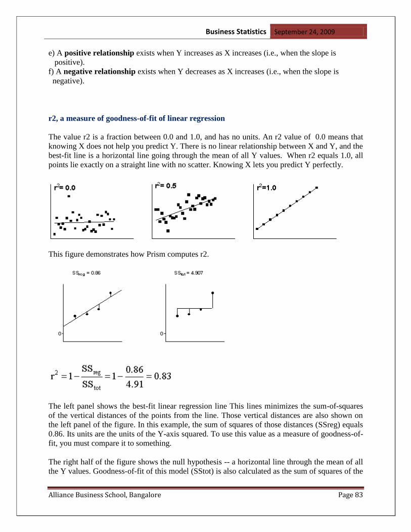
Business Statistics September 24, 2009
Alliance Business School, Bangalore Page 83
e) A positive relationship exists when Y increases as X increases (i.e., when the slope is
positive).
f) A negative relationship exists when Y decreases as X increases (i.e., when the slope is
negative).
r2, a measure of goodness-of-fit of linear regression
The value r2 is a fraction between 0.0 and 1.0, and has no units. An r2 value of 0.0 means that
knowing X does not help you predict Y. There is no linear relationship between X and Y, and the
best-fit line is a horizontal line going through the mean of all Y values. When r2 equals 1.0, all
points lie exactly on a straight line with no scatter. Knowing X lets you predict Y perfectly.
This figure demonstrates how Prism computes r2.
The left panel shows the best-fit linear regression line This lines minimizes the sum-of-squares
of the vertical distances of the points from the line. Those vertical distances are also shown on
the left panel of the figure. In this example, the sum of squares of those distances (SSreg) equals
0.86. Its units are the units of the Y-axis squared. To use this value as a measure of goodness-of-
fit, you must compare it to something.
The right half of the figure shows the null hypothesis -- a horizontal line through the mean of all
the Y values. Goodness-of-fit of this model (SStot) is also calculated as the sum of squares of the

Business Statistics September 24, 2009
Alliance Business School, Bangalore Page 84
vertical distances of the points from the line, 4.907 in this example. The ratio of the two sum-of-
squares values compares the regression model with the null hypothesis model. The equation to
compute r2 is shown in the figure. In this example r2 is 0.8248. The regression model fits the
data much better than the null hypothesis, so SSreg is much smaller than SStot, and r2 is near
1.0. If the regression model were not much better than the null hypothesis, r2 would be near zero.
You can think of r2 as the fraction of the total variance of Y that is "explained" by variation in X.
The value of r2 (unlike the regression line itself) would be the same if X and Y were swapped.
So r2 is also the fraction of the variance in X that is "explained" by variation in Y. In other
words, r2 is the fraction of the variation that is shared between X and Y.
In this example, 84% of the total variance in Y is "explained" by the linear regression model.
That leaves the rest of the vairance (16% of the total) as variability of the data from the model
(SStot)
The best fitting regression line: Least squares criterion
The formula for the least squares regression line is: Y Y Y ′ = b X + a
The most common version of the formula for the slope constant in least
squares regression is:
The ―Y‖ subscript on bY indicates that this is the slope for the regression of Y on X—that is for
the equation that allows prediction of Y-values from X-values.
SS is shorthand for the sum of the squared deviations about the
mean. The ―X‖ subscript indicates that it is the ―sum of squares‖ for the X-scores that we need.
The Regression Equation
[Standard notation: The data are pairs of independent and dependent variables {(xi,yi): i=1,...,n}.
The fitted equation is written is the predicted value of the response
obtained by using the equation. The residuals are the differences between the observed and the
predicted values . They are always calculated as (observed-predicted),
never the other way 'round.]

Business Statistics September 24, 2009
Alliance Business School, Bangalore Page 85
There are two primary reasons for fitting a regression equation to a set of data--first, to describe
the data; second, to predict the response from the carrier. The rationale behind the way the
regression line is calculated is best seen from the point-of-view of prediction. A line gives a good
fit to a set of data if the points are close to it. Where the points are not tightly grouped about any
line, a line gives a good fit if the points are closer to it than to any other line. For predictive
purposes, this means that the predicted values obtained by using the line should be close to the
values that were actually observed, that is, that the residuals should be small. Therefore, when
assessing the fit of a line, the vertical distances of the points to the line are the only distances that
matter. Perpendicular distances are not considered because errors are measured as vertical
distances, not perpendicular distances.
The simple linear regression equation is also called the least squares regression equation. Its
name tells us the criterion used to select the best fitting line, namely that the sum of the squares
of the residuals should be least. That is, the least squares regression equation is the line for which
the sum of squared residuals is a minimum.
It is not necessary to fit a large number of lines by trial-and-error to find the best fit. Some
algebra shows the sum of squared residuals will be minimized by the line for which
This can even be done by hand if need be.
When the analysis is performed by a statistical program package, the output will look something
like this.
A straight line can be fitted to any set of data. The formulas for the coefficients of the least
squares fit are the same for a sample, a population, or any arbitrary batch of numbers. However,

Business Statistics September 24, 2009
Alliance Business School, Bangalore Page 86
regression is usually used to let analysts generalize from the sample in hand to the population
from which the sample was drawn. There is a population regression equation,
0 + 1 X
and
Yi = 0 + 1 Xi + i,
where 0 and 1 are the population regression coefficients and i
is a random error peculiar to the i-th observation. Thus, each response is expressed as the sum of
a value predicted from the corresponding X, plus a random error.
The sample regression equation is an estimate of the population regression equation. Like any
other estimate, there is an uncertainty associated with it. The uncertainty is expressed in
confidence bands about the regression line. They have the same interpretation as the standard
error of the mean, except that the uncertainty varies according to the location along the line. The
uncertainty is least at the sample mean of the Xs and gets larger as the distance from the mean
increases. The regression line is like a stick nailed to a wall with some wiggle to it. The ends of
the stick will wiggle more than the center. The distance of the confidence bands from the
regression line is
,
where t is the appropriate percentile of the t distribution, se is the standard error of the estimate,
and x* is the location along the X-axis where the distance is being calculated. The distance is
smallest when x* = . These bands also
estimate the population mean value of Y
for X=x*.

Business Statistics September 24, 2009
Alliance Business School, Bangalore Page 87
There are also bands for predicting a single response at a particular value of X. The best estimate
is given, once again, by the regression line. The distance of the prediction bands from the
regression line is
.
For large samples, this is essentially tse, so the standard error of the estimate functions like a
standard deviation around the regression line.
The regression of X on Y is different
from the regression of Y on X. If
one wanted to predict lean body
mass from muscle strength, a new
model would have to be fitted
(dashed line). It could not be
obtained by taking the original
regression equation and solving for
strength. The reason is that in terms
of the original scatterplot, the best
equation for predicting lean body
mass minimizes the errors in the
horizontal direction rather than the
vertical. For example,
The regression of Strength
on LBM is
Strength = -13.971 + 3.016 LBM .
Solving for LBM gives
LBM = 4.632 + 0.332 Strength .
However, the regression of LBM on Strength is
LBM = 14.525 + 0.252 Strength .
The standard error of estimate:
There are in fact two such measures:
The variance error of estimate, and the standard error of estimate
The latter is the square root of the former. The standard error of estimate is to the least squares
regression line what the standard deviation is to the mean of a distribution.

Business Statistics September 24, 2009
Alliance Business School, Bangalore Page 88
The conceptual formula for the standard deviation of a distribution of Y-scores is given by:
The conceptual formula for the standard error of estimate when estimating Y given X is very
Similar.
Linear regression is used to predict a Y score from a score on X. Bear in mind the
following:
1) The relationship between X and Y must be linear. If the relationship is not linear,
prediction will not be very accurate.
2) Normally, we are not interested in predicting Y scores that are already known.
We derive our regression equation with sample data that consists of paired X and
Y scores, but use the equation to predict Y scores when only X values are given.
Because we use data collected from a sample to make these predictions, it is vital
to have a representative sample when deriving a regression equation.
3) A regression equation is properly used only for the range of the variables on
which it was based. We do not know whether the relationship between X and Y
continues to be linear beyond the range of sample values.
4) Prediction is most accurate if the data have the property of homoscedasticity—
i.e., if the variability of the Y scores is constant at all points along the regression
line.
5) When X and Y are both normally distributed and the number of paired scores is
large, the data in a bivariate frequency distribution often produce a so-called
bivariate normal distribution. When you have such a distribution, the standard
error of estimate can be used in the same way we used the standard deviation of
a normal distribution. That is, we could say that about 68% of the scores in the
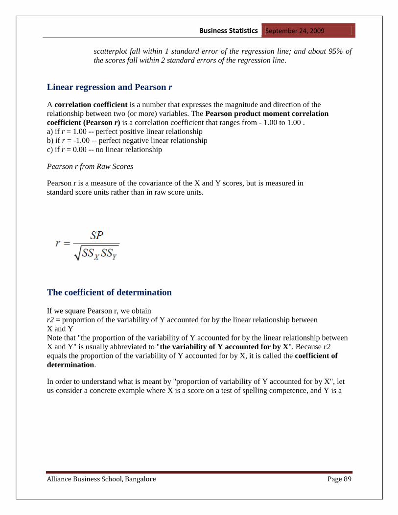
Business Statistics September 24, 2009
Alliance Business School, Bangalore Page 89
scatterplot fall within 1 standard error of the regression line; and about 95% of
the scores fall within 2 standard errors of the regression line.
Linear regression and Pearson r
A correlation coefficient is a number that expresses the magnitude and direction of the
relationship between two (or more) variables. The Pearson product moment correlation
coefficient (Pearson r) is a correlation coefficient that ranges from - 1.00 to 1.00 .
a) if r = 1.00 -- perfect positive linear relationship
b) if r = -1.00 -- perfect negative linear relationship
c) if r = 0.00 -- no linear relationship
Pearson r from Raw Scores
Pearson r is a measure of the covariance of the X and Y scores, but is measured in
standard score units rather than in raw score units.
The coefficient of determination
If we square Pearson r, we obtain
r2 = proportion of the variability of Y accounted for by the linear relationship between
X and Y
Note that "the proportion of the variability of Y accounted for by the linear relationship between
X and Y" is usually abbreviated to "the variability of Y accounted for by X". Because r2
equals the proportion of the variability of Y accounted for by X, it is called the coefficient of
determination.
In order to understand what is meant by "proportion of variability of Y accounted for by X", let
us consider a concrete example where X is a score on a test of spelling competence, and Y is a
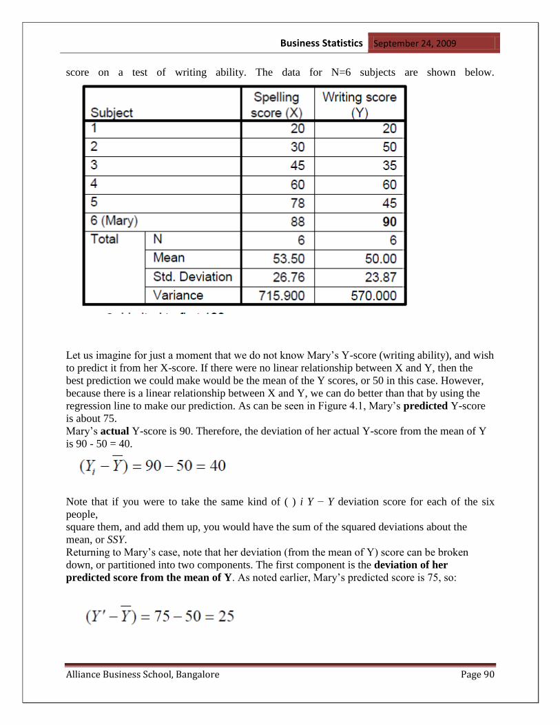
Business Statistics September 24, 2009
Alliance Business School, Bangalore Page 90
score on a test of writing ability. The data for N=6 subjects are shown below.
Let us imagine for just a moment that we do not know Mary‘s Y-score (writing ability), and wish
to predict it from her X-score. If there were no linear relationship between X and Y, then the
best prediction we could make would be the mean of the Y scores, or 50 in this case. However,
because there is a linear relationship between X and Y, we can do better than that by using the
regression line to make our prediction. As can be seen in Figure 4.1, Mary‘s predicted Y-score
is about 75.
Mary‘s actual Y-score is 90. Therefore, the deviation of her actual Y-score from the mean of Y
is 90 - 50 = 40.
Note that if you were to take the same kind of ( ) i Y − Y deviation score for each of the six
people,
square them, and add them up, you would have the sum of the squared deviations about the
mean, or SSY.
Returning to Mary‘s case, note that her deviation (from the mean of Y) score can be broken
down, or partitioned into two components. The first component is the deviation of her
predicted score from the mean of Y. As noted earlier, Mary‘s predicted score is 75, so:

Business Statistics September 24, 2009
Alliance Business School, Bangalore Page 91
The second component of the deviation of Mary‘s actual score from the mean of Y is the
deviation of her actual score from her predicted score:

Business Statistics September 24, 2009
Alliance Business School, Bangalore Page 92
CORRELATION
Definitions: Correlation is a statistical technique that is used to measure a relationship
between two variables. Correlation requires two scores from each individual (one score from
each of the two variables)
Distinguishing Characteristics of Correlation
Correlation procedures involve one sample containing all pairs of X and Y scores
Neither variable is called the independent or dependent variable
Use the individual pair of scores to create a scatterplot
Sum of Product Deviations
In the past you have used the sum of squares or SS to measure the amount of variation or
variability for a single variable The sum of products or SP provides a parallel procedure for
measuring the amount of covariation or covariability between two variables

Business Statistics September 24, 2009
Alliance Business School, Bangalore Page 93
Covariance
A measure of the linear association between variables
Positive indicates positive linear relationship
Negative indicates a negative linear relationship
Values close to zero indicates no linear relationship
It is dependent upon the units of measurement for x and y variables
Height in inches would give a larger covariance than height in feet; even with same
degree of association
So the magnitude of the covariance is not significant
Covariance Formula

Business Statistics September 24, 2009
Alliance Business School, Bangalore Page 94
Covariance Example
Correlation Coefficient Formula 1

Business Statistics September 24, 2009
Alliance Business School, Bangalore Page 95
Correlation Coefficient Formula 2
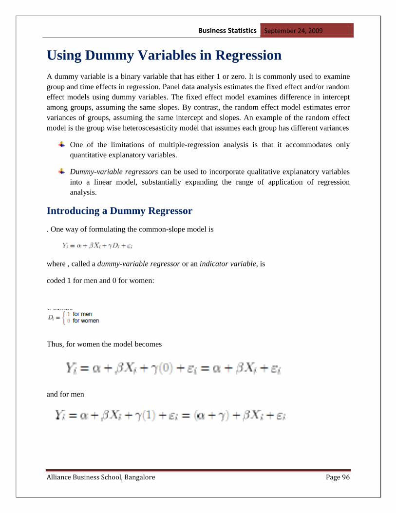
Business Statistics September 24, 2009
Alliance Business School, Bangalore Page 96
Using Dummy Variables in Regression
A dummy variable is a binary variable that has either 1 or zero. It is commonly used to examine
group and time effects in regression. Panel data analysis estimates the fixed effect and/or random
effect models using dummy variables. The fixed effect model examines difference in intercept
among groups, assuming the same slopes. By contrast, the random effect model estimates error
variances of groups, assuming the same intercept and slopes. An example of the random effect
model is the group wise heteroscesasticity model that assumes each group has different variances
One of the limitations of multiple-regression analysis is that it accommodates only
quantitative explanatory variables.
Dummy-variable regressors can be used to incorporate qualitative explanatory variables
into a linear model, substantially expanding the range of application of regression
analysis.
Introducing a Dummy Regressor
. One way of formulating the common-slope model is
where , called a dummy-variable regressor or an indicator variable, is
coded 1 for men and 0 for women:
Thus, for women the model becomes
and for men

Business Statistics September 24, 2009
Alliance Business School, Bangalore Page 97
How and Why Dummy Regression Works
Interpretation of parameters in the additive dummy-regression model: gives the difference in
intercepts for the two regression lines.Because these regression lines are parallel, also represents
the constant separation between the lines — the expected income advantage accruing to men
when education is held constant.
If men were disadvantaged relative to women, then would be negative.
gives the intercept for women, for whom = 0.
is the common within-gender education slope.
Figure 3 reveals the fundamental geometric ‗trick‘ underlying the coding of a dummy regressor:
We are, in fact, fitting a regression plane to the data, but the dummy regressor is defined only at
the values zero and one

Business Statistics September 24, 2009
Alliance Business School, Bangalore Page 98
Many Categories

Business Statistics September 24, 2009
Alliance Business School, Bangalore Page 99
EXAMPLE 2
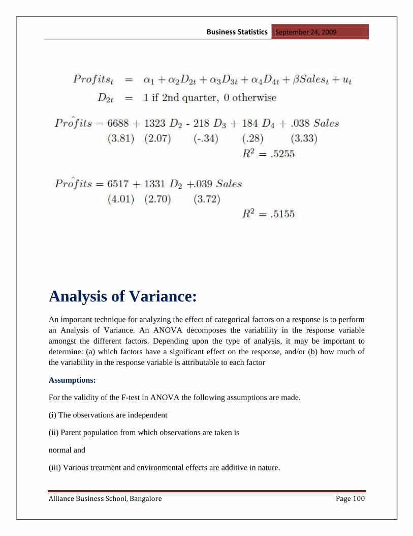
Business Statistics September 24, 2009
Alliance Business School, Bangalore Page 100
Analysis of Variance:
An important technique for analyzing the effect of categorical factors on a response is to perform
an Analysis of Variance. An ANOVA decomposes the variability in the response variable
amongst the different factors. Depending upon the type of analysis, it may be important to
determine: (a) which factors have a significant effect on the response, and/or (b) how much of
the variability in the response variable is attributable to each factor
Assumptions:
For the validity of the F-test in ANOVA the following assumptions are made.
(i) The observations are independent
(ii) Parent population from which observations are taken is
normal and
(iii) Various treatment and environmental effects are additive in nature.

Business Statistics September 24, 2009
Alliance Business School, Bangalore Page 101
One way Classification:
Let us suppose that N observations xij , i = 1, 2, …… k ;j = 1,2….ni) of a random variable X are
grouped on some basis,into k classes of sizes n1, n2 , …..nk respectively
exhibited below
Test Procedure:
The steps involved in carrying out the analysis are:
1) Null Hypothesis:
The first step is to set up of a null hypothesis
H0: 1 = 2 = …= k
Alternative hypothesis H1: all i ‗ s are not equal (i = 1,2,…,k)
2) Level of significance : Let : 0.05

Business Statistics September 24, 2009
Alliance Business School, Bangalore Page 102
3) Test statistic:
Various sum of squares are obtained as follows.
a) Find the sum of values of all the (N) items of the given data. Let this grand total represented
by ‗ G‘ .Then correction factor
b) Find the sum of squares of all the individual items (xij)and then the Total sum of squares
(TSS) is
c) Find the sum of squares of all the class totals (or each treatment total) Ti (i:1,2,….k) and then
the sum of squares between the classes or between the treatments
(SST) is
Where ni (i: 1,2,…..k) is the number of observations in the ith class or number of observations
received by ith treatment
d) Find the sum of squares within the class or sum of squares due to error (SSE) by subtraction.
SSE = TSS - SST
4) Degrees of freedom (d.f):
The degrees of freedom for total sum of squares (TSS) is (N1). The degrees of freedom for SST
is (k1) and the degrees of freedom for SSE is (Nk)
5) Mean sum of squares:
The mean sum of squares for treatments is and meansum of squares for error is
6) ANOVA Table
The above sum of squares together with their respective degrees of freedom and mean sum of
squares will be summarized in the following table.

Business Statistics September 24, 2009
Alliance Business School, Bangalore Page 103
Calculation of variance ratio:
Variance ratio of F is the ratio between greater variance and smaller variance, thus
F = Variance between the treatments Variance within the treatment = MST/MSE
If variance within the treatment is more than the variance between the treatments, then numerator
and denominator should be interchanged and degrees of freedom adjusted accordingly.
7) Critical value of F or Table value of F:
The Critical value of F or table value of F is obtained from F table for (k-1, N-k) d.f at 5% level
of significance.
8) Inference:
If calculated F value is less than table value of F, we may accept our null hypothesis H0 and say
that there is no significant difference between treatments. If calculated F value is greater than
table value of F, we reject our H0 and say that the difference between treatments is significant.

Business Statistics September 24, 2009
Alliance Business School, Bangalore Page 104
Example 1:
SQUARES

Business Statistics September 24, 2009
Alliance Business School, Bangalore Page 105

Business Statistics September 24, 2009
Alliance Business School, Bangalore Page 106

Business Statistics September 24, 2009
Alliance Business School, Bangalore Page 107

Business Statistics September 24, 2009
Alliance Business School, Bangalore Page 108

Business Statistics September 24, 2009
Alliance Business School, Bangalore Page 109

Business Statistics September 24, 2009
Alliance Business School, Bangalore Page 110

Business Statistics September 24, 2009
Alliance Business School, Bangalore Page 111
EXAMPLE

Business Statistics September 24, 2009
Alliance Business School, Bangalore Page 112

Business Statistics September 24, 2009
Alliance Business School, Bangalore Page 113

Business Statistics September 24, 2009
Alliance Business School, Bangalore Page 114
Time series
Introduction: Arrangement of statistical data in chronological order i.e., in accordance with
occurrence of time, is known as ―Time Series‖. Such series have a unique important place in the
field of Economic and Business statistics. An economist is interested in estimating the likely
population in the coming year so that proper planning can be carried out with regard to food
supply, job for the people etc.
Similarly; a business man is interested in finding out his likely sales in the near future, so that the
businessman could adjust his production accordingly and avoid the possibility of inadequate
production to meet the demand. In this connection one usually deal with statistical data, which
are collected, observed or recorded at successive intervals of time. Such data are generally
referred to as‗time series‘.
Definition: A time series is a set of statistical observations arranged in chronological order.A
time series may be defined as a collection of readings belonging to different time periods, of
some economic variable or composite of variables. A time series is a set of observations of a
variable usually at equal intervals of time. Here time may be yearly, monthly, weekly, daily or
even hourly usually at equal intervals of time. Hourly temperature reading, daily sales, monthly
production are examples of time series
Components of Time series:
The components of a time series are the various elements which can be segregated from the
observed data. The following are the broad classification of these components.

Business Statistics September 24, 2009
Alliance Business School, Bangalore Page 115
In time series analysis, it is assumed that there is a multiplicative relationship between these four
components. Symbolically, Y = T S C I Where Y denotes the result of the four elements; T
= Trend ; S = Seasonal component; C = Cyclical components; I = Irregular component .In the
multiplicative model it is assumed that the four components are due to different causes but they
are not necessarily independent and they can affect one another.
Another approach is to treat each observation of a time
series as the sum of these four components. Symbolically
Y = T + S+ C+ I
The additive model assumes that all the components of the time series are independent of one
another.
1) Secular Trend or Long - Term movement or simply Trend
2) Seasonal Variation
3) Cyclical Variations
4) Irregular or erratic or random movements (fluctuations)
Secular Trend:
It is a long term movement in Time series. The general tendency of the time series is to increase
or decrease or stagnate during a long period of time is called the secular trend or simply trend.
Population growth, improved technological progress, changes in consumers taste are the various
factors of upward trend. We may notice downward trend relating to deaths, epidemics, due to
improved medical facilities and sanitations. Thus a time series shows fluctuations in the upward
or downward direction in the long run.
Methods of Measuring Trend:
Trend is measured by the following mathematical methods.
1. Graphical method
2. Method of Semi-averages
3. Method of moving averages
4. Method of Least Squares
Graphical Method:
This is the easiest and simplest method of measuring trend. In this method, given data must be
plotted on the graph, taking time on the horizontal axis and values on the vertical axis. Draw a
smooth curve which will show the direction of the trend. While fit ting a trend line the following
important points should be noted to get a perfect trend line.
The curve should be smooth.
As far as possible there must be equal number of points above and below the trend line.
The sum of the squares of the vertical deviations from the trend should be as small as
possible.

Business Statistics September 24, 2009
Alliance Business School, Bangalore Page 116
If there are cycles, equal number of cycles should be
above or below the trend line.
In case of cyclical data, the area of the cycles above and below should be nearly equal.

Business Statistics September 24, 2009
Alliance Business School, Bangalore Page 117
EXAMPLE
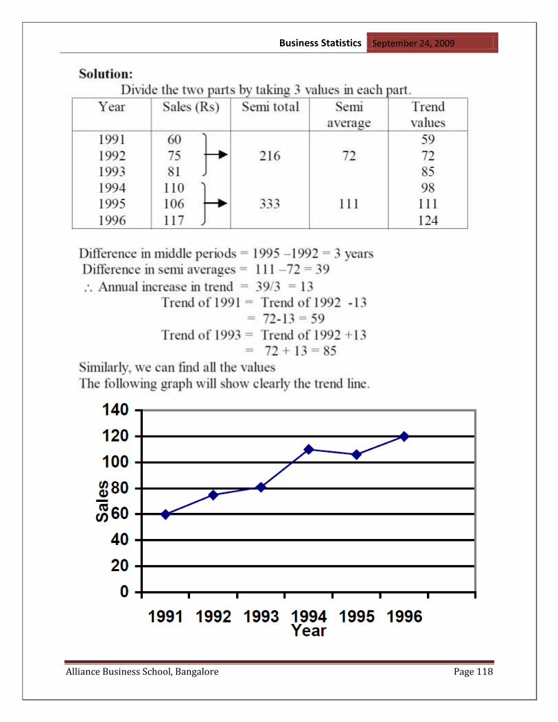
Business Statistics September 24, 2009
Alliance Business School, Bangalore Page 118

Business Statistics September 24, 2009
Alliance Business School, Bangalore Page 119
Merits:
1. It is simple and easy to calculate
2. By this method every one getting same trend line.
3. Since the line can be extended in both ways, we can find the later and earlier estimates.
Demerits:
1. This method assumes the presence of linear trend to the values of time series which may not
exist.
2. The trend values and the predicted values obtained by this method are not very reliable.

Business Statistics September 24, 2009
Alliance Business School, Bangalore Page 120
EXAMPLE
Even Period of Moving Averages:
When the moving period is even, the middle period of each set of values lies between the two
time points. So we must center the moving averages.
The steps are
Find the total for first 4 years and place it against the middle of the 2nd and 3rd year in
the third column.
Leave the first year value, and find the total of next four-year and place it between the 3rd
and 4th year.

Business Statistics September 24, 2009
Alliance Business School, Bangalore Page 121
Continue this process until the last value is taken.
Next, compute the total of the first two four year totals and place it against the 3rd year in
the fourth column.
Leave the first four years total and find the total of the next two four years‘ totals and
place it against the fourth year.
This process is continued till the last two four years‘ total is taken into account.
Divide this total by 8 (Since it is the total of 8 years) and put it in the fifth column.
These are the trend values.
EXAMPLE The production of Tea in India is given as follows. Calculate the Four-yearly moving averages

Business Statistics September 24, 2009
Alliance Business School, Bangalore Page 122
Merits:
The method is simple to understand and easy to adopt as compared to other methods.
It is very flexible in the sense that the addition of a few more figures to the data, the
entire calculations is not changed. We only get some more trend values.
Regular cyclical variations can be completely eliminated by a period of moving average
equal to the period of cycles
It is particularly effective if the trend of a series is very irregular.
Demerits:
It cannot be used for forecasting or predicting future trend,which is the main objective of
trend analysis
The choice of the period of moving average is sometimes subjective.
Moving averages are generally affected by extreme values of items.
It cannot eliminate irregular variations completely.
METHOD OF LEAST SQUARE:

Business Statistics September 24, 2009
Alliance Business School, Bangalore Page 123
EXAMPLE

Business Statistics September 24, 2009
Alliance Business School, Bangalore Page 124

Business Statistics September 24, 2009
Alliance Business School, Bangalore Page 125

Business Statistics September 24, 2009
Alliance Business School, Bangalore Page 126
Merits:
Since it is a mathematical method, it is not subjective so it eliminates personal bias of the
investigator.
By this method we can estimate the future values. As well as intermediate values of the
time series.
By this method we can find all the trend values.
Demerits:
It is a difficult method. Addition of new observations makes recalculations.
Assumption of straight line may sometimes be misleading since economics and business
time series are not linear.
It ignores cyclical, seasonal and irregular fluctuations.
The trend can estimate only for immediate future and not for distant future.
XBAR

Business Statistics September 24, 2009
Alliance Business School, Bangalore Page 127
Graphics Commands XBAR CHART DATAPLOT Reference Manual March 11, 1997 2-273
XBAR CHART
PURPOSE
Generates a mean control chart.
DESCRIPTION
An xbar (or mean) control chart is a data analysis technique for determining if a measurement
process has gone out of statistical control. The xbar chart is sensitive to shifts in location in the
measurement process.
It consists of:
Vertical axis = the mean for each sub-group.
Horizontal axis = sub-group designation.
In addition, horizontal lines are drawn at the overall mean and at the upper and lower control
limits. The distribution of the response variable is assumed to be normal. This assumption is the
basis for calculating the upper and lower control limits.
SYNTAX
XBAR CHART <y> <x> <SUBSET/EXCEPT/FOR qualification>
where <y> is the response (= dependent) variable (containing the raw data values);
<x> is an independent variable (containing the sub-group identifications);
and where the <SUBSET/EXCEPT/FOR qualification> is optional.
EXAMPLES
XBAR CHART Y X
XBAR CHART Y X SUBSET X > 2
NOTE
The attributes of the 4 traces can be controlled by the standard LINES, CHARACTERS, BARS,
and SPIKES commands. Trace 1 is the response variable, trace2 is the mean line, and traces 3
and 4 are the control limits. Some analysts prefer to draw the response variable as a spike or
character rather than a connected line.
DEFAULT
None
SYNONYMS
XBAR CONTROL CHART, MEAN CONTROL CHART, MEAN CHART, X CHART,
AVERAGE CONTROL CHART, and
AVERAGE CHART are synonyms for XBAR CHART.
RELATED COMMANDS
R CHART = Generates a range control chart.
S CHART = Generates a standard deviation control chart.
P CHART = Generates a p control chart.

Business Statistics September 24, 2009
Alliance Business School, Bangalore Page 128
NP CHART = Generates a Np control chart.
U CHART = Generates a U control chart.
C CHART = Generates a C control chart.
Q CONTROL CHART = Generates a Quesenberry style control chart.
CHARACTERS = Sets the types for plot characters.
LINES = Sets the types for plot lines.
SPIKES = Sets the on/off switches for plot spikes.
BARS = Sets the on/off switches for plot bars.
PLOT = Generates a data or function plot.
LAG PLOT = Generates a lag plot.
4-PLOT = Generates 4-plot univariate analysis.
MEAN PLOT = Generates a mean versus subset plot.
APPLICATIONS
Quality Control
IMPLEMENTATION DATE
88/2
XBAR CHART Graphics Commands
2-274 March 11, 1997 DATAPLOT Reference Manual
PROGRAM
SKIP 25
READ GEAR.DAT DIAMETER BATCH
.
LINE SOLID SOLID DOT DOT
TITLE AUTOMATIC
X1LABEL GROUP-ID
Y1LABEL MEAN
X CHART DIAMETER BATCH
1 2 3 4 5 6 7 8 9 10
0.99
0.995
1
1.005
1.01
XBAR CHART DIAMETER BATCH
GROUP-ID
MEAN XBAR

Business Statistics September 24, 2009
Alliance Business School, Bangalore Page 129

Business Statistics September 24, 2009
Alliance Business School, Bangalore Page 130