Embed Size (px)
Citation preview

Volume 8, Number 2 Print ISSN 1944-656X
Online ISSN 1944-6578
BUSINESS STUDIES JOURNAL
Editor
Dr. Marty Ludlum
University of Central Oklahoma
The official journal of the Academy for
Business Studies, an Affiliate of the
Allied Academies
The Business Studies Journal is owned and published by Jordan Whitney Enterprises, Inc.
Editorial content is under the control of the Allied Academies, Inc., a non-profit association of
scholars, whose purpose is to support and encourage research and the sharing and exchange of
ideas and insights throughout the world.
Authors execute a publication permission agreement and assume all liabilities. Neither
Jordan Whitney Enterprises nor Allied Academies is responsible for the content of the
individual manuscripts. Any omissions or errors are the sole responsibility of the
authors. The Editorial Board is responsible for the selection of manuscripts for
publication from among those submitted for consideration. The Publishers accept final
manuscripts in digital form and make adjustments solely for the purposes of pagination
and organization.
The Business Studies Journal is owned and published by Jordan Whitney Enterprises,
Inc., PO Box 1032, Weaverville, NC 28787, USA. Those interested in communicating
with the Journal, should contact the Executive Director of the Allied Academies at
Copyright 2016 by Jordan Whitney Enterprises, Inc., USA

EDITORIAL REVIEW BOARD
Ismet Anitsal Bill Christensen
Tennessee Tech University Dixie State University
Suzanne Lay Steven V. Cates
Colorado Mesa University Kaplan University
Jeffrey Barnes M. Meral Anitsal
Southern Utah University Tennessee Tech Universty
Ramaswamy Ganesan Lewis Hershey
King Saud University Fayetteville State University
Jeff Jewell Marvin P. Ludlum
Lipscomb University University of Central Oklahoma
Vivek Shankar Natarajan Sanjay Rajagopal
Lamar University Western Carolina University
Durga Prasad Samontaray David Smarsh
King Saud University Trident University International
Cazimir Barczyk James Frost
Purdue University Calumet Idaho State University
Gerald Calvasina
Southern Utah University

TABLE OF CONTENTS
COMMUNITY INVOLVEMENT AND THE HOMETOWN EFFECT: A FACTOR IN FAMILY BUSINESS
EXPANSION PATTERNS…………………………………………………………………………………………1
Marilyn Young, The University of Texas at Tyler
John James Cater III, The University of Texas at Tyler
A JOURNEY FROM A SERVICE LEARNING PROJECT TO AN ACADEMIC-COMMUNITY
COLLABORATION EFFORT……………………………………………………………………………………..9
Minh Huynh, Southeastern Louisiana University
DOES TRANSFORMATION LEADERSHIP PROMOTE INNOVATION PRACTICES IN E-
COMMERCE?.........................................................................................................................................................30
Dr. Joe Ilsever, University of the Fraser Valley
Omar Ilsever, Our Lady of the Lake University
IMPLIED VERSUS REALIZED VOLATILITY OF S&P 500: EFFECTS OF STOCK MARKET
FACTORS………………………………………………………………………………………………………...36
Andrey Kudryavtsev, The Max Stern Yezreel Valley Academic College
WHAT IS WRONG WITH INDIAN CORPORATE GOVERNANCE? : A CASE STUDY OF FAILURE OF
KINGFISHER AIRLINES………………………………………………………………………………………...46
Siva Prasad Ravi, Thompson Rivers University
THE KEY INDICATORS OF GOODWILL IMPAIRMENT WRITE-OFFS……………………………………63
Karen Sherrill, Sam Houston State University
FOUR PROOFS IN OPTION PRICING………………………………………………………………………….72
Garland Simmons, Stephen F. Austin State University
THE LECTURE/LAB COMBINATION COURSE: AN INNOVATIVE WAY TO TEACH A LARGE
WRITING COURSE…………………………………………………………………………………………...…88
Dr. Carol S. Wright, Stephen F. Austin State University
A MODEL OF BUSINESS PERFORMANCE IN THE US AIRLINE INDUSTRY: HOW CUSTOMER
COMPLAINTS PREDICT THE PERFORMANCE?.............................................................................................96
Sule Birim, Manisa Celal Bayar University
M. Meral Anitsal, Tennessee Tech University
İsmet Anitsal, Tennessee Tech University
DESIGN OF PROCEDURAL CONSTRAINTS: CASE STUDY BASED ON PARTICIPANT OBSERVATION
REGARDING MANAGEMENT OF EMPLOYEE CREATIVITY……………………………………………112
Masato Fujii, Kobe University
EXPLORING GREEN ENERGY PRODUCTION AND SUPPLY CHAIN ISSUES………………………….123
Kelly Weeks, Lamar University
ACCEPTABLE CHEATING BEHAVIORS?.......................................................................................................139
Wendy C. Bailey, Troy University
S. Scott Bailey, Troy University
Connie Nott, Troy University
Business Studies Journal Volume 8, Number 2, 2016
1
COMMUNITY INVOLVEMENT AND THE HOMETOWN
EFFECT: A FACTOR IN FAMILY BUSINESS
EXPANSION PATTERNS
Marilyn Young, The University of Texas at Tyler
John James Cater III, The University of Texas at Tyler
ABSTRACT
The purpose of this study was to examine community involvement among family businesses
as related to their growth and expansion. One success factor may be their strong community
relationships and reputation, since owners believe that the local hometown is part of their success
and want to “give back.” The family businesses interviewed were very active in their communities
and had a strong sense of community values. These activities include donations, sponsorships,
serving on boards of directors, and others. It is possible that family businesses involved in the
local community will become dependent on the hometown and, therefore, not venture outside the
local geographic area. These firms may perceive that their success is centered in a single
geographical area and still remaining successful. We propose that family business involvement
and close community ties could ultimately affect their growth and expansion efforts. This
qualitative study is based upon interviews with seven small businesses.
INTRODUCTION
Family businesses tend to be involved in their local communities, which include
memberships in civic groups, churches, schools, and other nonprofit organizations. Past studies
have shown that family business success factors include having quality products and services,
product differentiation strategies, and the founder’s intent and vision. However, another success
factor may be the strong ties to the hometown and the local reputation of the firm. Therefore, the
purpose of this study is to examine community involvement among family businesses and its
effect on growth patterns and expansion.
It is often said that many small businesses and family-owned firms tend to be close to their
communities. These strong ties include involvement in nonprofit organizations and memberships
in civic groups, such as Rotary International, Chambers of Commerce, and Better Business
Bureaus. Other participation and support include religious, educational, civic, and other
institutions.
The primary focus of this study was to examine the importance of the “hometown” effect
as it relates to social responsibility and growth strategies. Although much research has been
conducted regarding social responsibility and business strategies, this study examines community
involvement as an important aspect of family business success. This research effort consists of
personal interviews with firms that represent a variety of businesses. These firms were selected
from the following industries: general retail, furniture, auto repair, restaurant, health foods,
convenience, and auto parts.

Business Studies Journal Volume 8, Number 2, 2016
2
Specifically, this research asked the following questions:
1. What types of community activities do family businesses support and participate?
2. How important is local community involvement to the family businesses and what types of
community values exist.
3. Are these strong ties to the hometown and local area related to business expansion and
growth?
SURVEY OF LITERATURE
The literature supports the idea that family businesses desire to be involved their
communities. Also, much of the literature shows how family businesses are involved in the
community in terms of “giving back,” the importance of social responsibility, and motives for
community support. However, no studies have related family firms that remain in the local area
and choose not to expand due to their ties to the local community culture, values, and
relationships.
Community Relationships
One study examined several factors involved in business and community involvement. The
research was a qualitative study of 52 small- to medium-sized enterprises (SMEs) in Australia and
examined motives, methods, and obstacles toward community participation (Madden, Schaife, &
Crissman, 2006).
The SMEs preferred to avoid cash gifts but desired to support local causes. A major motive
was a genuine belief that business organizations should support community causes. By the same
token, the community expected that the enterprises would play an active part in the community. In
addition, the firms indicated that this community participation would benefit their businesses.
(Madden, Schaife, & Crissman, 2006).
A recent study examined small businesses and their interests in nonprofit collaboration
(Zatepillina-Monacell, 2015). In utilizing interviews and focus groups, the researcher concluded
that small businesses were interested in serving on nonprofit boards. Specifically, these small
businesses wanted to support those nonprofit organizations that helped and provided assistance to
the needs of the community. Moreover, the small businesses were interested in long-term
partnerships with nonprofit organizations that focused on local community issues.
Family Business Growth
Factors affecting growth and strategic planning in the small business literature are
widespread. Eddleston et al. (2013) analyzed factors in strategic planning and argued the
importance of analyzing strategic planning efforts in light of different generations. They
suggested that growth, strategic planning, and succession planning are affected by the
management of first, second, or generations beyond (Eddleston, Kellermanns, Floyd, Crittenden,
& Crittenden, 2013). However, research studies on success factors and growth strategies are
limited when community involvement is involved.
Hamelin (2013) suggested that financing capacity might be explained in growth patterns
between family and non-family businesses. Further, he indicated that family involvement could
intentionally limit their growth. It is possible that this involvement could lead to atypical
behavior, and thus these businesses may implement conservative growth patterns. In addition, he

Business Studies Journal Volume 8, Number 2, 2016
3
pointed out that firm financing capacity, as well as and other factors, could limit growth (Hamlin,
2013).
Community Culture
Astrachan (1988) recognized early on the importance of the community related to small
business success while examining a family firm case study. He reported that when small
businesses are in harmony and/or compatible with the local culture, a higher level of morale and
long-term productivity may follow. Ideally, family firms tend to be more congruent with the
community culture. The family firms may have a strong sense of community and, therefore,
encourage employees to be involved in local committees. The owner in the study believed that
the company would be a substantial asset to the city and the community and pointed out that the
community should even own and control the stock in the local institution (Astrachan, 1988).
After interviewing a successful four-generation family business, Karofsky (2001)
suggested that public service involvement was important and deeply engrained in the family
culture. In his interview, Grossman of Massachusetts further indicated that a challenge existed
for individuals while balancing a family, career, and community participation.
Small Businesses and Support of Community
The enlightened self-interest model of business and social responsibility suggests that
businesses can realize significant benefits through socially responsible behavior (Besser &
Miller, 2004). They stated the roles of small businesses in the community have received limited
attention in the business social responsibility literature. Yet, they found that supporting the
community was an important strategy for business success. In other words, a good public image
was perceived to be important for business success. This finding was true for both non-risky and
risky support.
Community Influence on Family Business Involvement
Family businesses appear to have significant ties to the community which, therefore,
could explain their lack of expansion (Fitzgerald, Haynes, Schrank, & Danes, 2010). In
surveying family businesses, researchers found that social and economic factors affecting the
community may contribute to business performance and responsible actions. The National
Family Business Survey reported that family businesses with positive attitudes toward local
communities were more likely to serve in leadership positions and contribute to the community.
Further, they found that family businesses were willing to accept leadership positions and
contribute in the form of technical expertise and financial assistance when the economy was at
risk.
Success and Social Responsibility
Besser (1999) examined the relationship between the success of small businesses and
social responsibility of firms in Iowa. He found that small businesses in small towns reported
high levels of commitment and support for the community. He defined social responsibility as a
commitment and support for the community. In using multiple regression analysis, he showed
that helpful corporate citizenship was also good for the businesses. He concluded, “As a result of
their positive net association with business success, commitment to the community and

Business Studies Journal Volume 8, Number 2, 2016
4
providing support for the community may be considered strategies for business success”
(Bessler, 1999, p. 27). In addition, his findings showed an interdependency between businesses
and their local communities.
In addition, Bessler (2012) examined motivations of small business regarding their
contribution to the community. In analyzing the consequences for their involvement in the
community, he stated, “The town where they do business is their home. Their personal well-
being, and, often, the success of their business are inextricably linked to the overall welfare of
the community” (Bessler (2012, p. 131).
Another study gave credence to the fact that small businesses are motivated to be socially
responsible. Udayaskankar (2008) reported that small- and medium-sized firms comprise 90% of
the worldwide business population. Although it has been suggested that given their smaller scale,
access to resources and lower visibility, smaller firms were less likely to participate in social
responsible initiatives. While examining different motivations of firms, he found that both very
small and very large firms were equally motivated. Moreover, medium-sized firms were the least
motivated, which illustrates that a U-shaped relationship between firm size and social
responsibility participation occurs. However, he pointed out that when broad categories of
businesses are sampled, caution should be taken.
Reciprocated Community Support
In a study of 800 small businesses in small towns in Iowa, researchers reported findings
regarding reciprocity between small businesses and the community. In particular, entrepreneurs
who made contributions to their community perceived themselves to be successful. In addition,
the study showed that the interaction effect of an entrepreneur's service to the community and
reciprocated by community support of the business was the single most significant determinant
of business success among many variables and respondent characteristics. Moreover, an
important finding was the belief that individuals who felt successful expect to expand (Kilkenny,
Nalbarte, & Besser, 1999).
Regional Influences on Startups
Bird (2014) investigated how regional factors impacted family and non-family startups.
The study was based on longitudinal data and showed economic factors, such as population and
regional growth, to be primarily associated with the number of non-family start-up businesses.
However, factors related to regional embeddedness, such as pre-existing small family businesses
and favorable community attitudes toward small businesses, were more strongly associated with
the number of family start-ups. They suggested that this regional factor was an important area for
family business and start-up research.
Survival of Family Firms
Santarelli and Lotti (2015) found problems of growth and succession to be a major cause
in family firm closures. In addition, they reported small family firms that had reached 30 years
in existence had a very high risk of sudden exit. Likewise, this potential risk increased with the
age of the firm.
Business Studies Journal Volume 8, Number 2, 2016
5
METHODS OF RESEARCH
This research effort consisted of personal interviews with seven family businesses to
examine their perceptions on many factors. For this study, we focused, in particular, on the
understanding of family businesses and their relationships and partnerships with local
community activities. The questionnaire was carefully developed with input from other studies.
The questionnaire was designed to obtain open-ended answers and organized into the following
general categories: Firm history and description, challenges, family dynamics, expansion
patterns, and succession plans. Initially, interviewing was conducted with one of the owner
during the spring, 2015; however, interviews were repeated with different family members in
order to obtain more in-depth experiences.
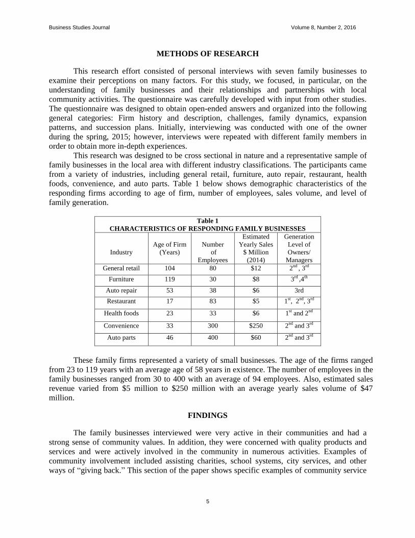
This research was designed to be cross sectional in nature and a representative sample of
family businesses in the local area with different industry classifications. The participants came
from a variety of industries, including general retail, furniture, auto repair, restaurant, health
foods, convenience, and auto parts. Table 1 below shows demographic characteristics of the
responding firms according to age of firm, number of employees, sales volume, and level of
family generation.
Table 1
CHARACTERISTICS OF RESPONDING FAMILY BUSINESSES
Industry
Age of Firm
(Years)
Number
of
Employees
Estimated
Yearly Sales
$ Million
(2014)
Generation
Level of
Owners/
Managers
General retail 104 80 $12 2nd
, 3rd
Furniture 119 30 $8 3rd
,4th
Auto repair 53 38 $6 3rd
Restaurant 17 83 $5 1st, 2
nd, 3
rd
Health foods 23 33 $6 1st and 2
nd
Convenience 33 300 $250 2nd
and 3rd
Auto parts 46 400 $60 2nd
and 3rd
These family firms represented a variety of small businesses. The age of the firms ranged
from 23 to 119 years with an average age of 58 years in existence. The number of employees in the
family businesses ranged from 30 to 400 with an average of 94 employees. Also, estimated sales
revenue varied from $5 million to $250 million with an average yearly sales volume of $47
million.
FINDINGS
The family businesses interviewed were very active in their communities and had a
strong sense of community values. In addition, they were concerned with quality products and
services and were actively involved in the community in numerous activities. Examples of
community involvement included assisting charities, school systems, city services, and other
ways of “giving back.” This section of the paper shows specific examples of community service

Business Studies Journal Volume 8, Number 2, 2016
6
participation by family businesses in their hometown. These finding led to the following
proposition:
Family business involvement with their close community relationships and
hometown could ultimately affect their growth and expansion efforts.
Community Involvement
One major community involvement activity was the association with religious
institutions. One restaurant owner stated, “We are very involved in church activities. Many
people come in after church, since the restaurant is next door. We have done a lot of business
with them for years and know the pastors.”
Also, these businesses have a close relationship with educational institutions, since many
were raised in their local communities and went to area schools. Also, companies mentioned that
their friends and relatives also went to the hometown schools. In fact, many owners started they
started working in the family businesses after school.
Community Awareness
Another example of community involvement was having local community leaders serve
on their boards of directors. One individual indicated that a hometown doctor was on the boards
of directors of his organization. Another owner stated, “This community is our home, and our
customers are our neighbors. We want to give quality service to our customers.”
Customer Care
An auto repair shop owner wanted their hometown customers to feel comfortable and,
therefore, created an atmosphere that does not resemble a “typical auto repair shop.” For
example, the shop is very clean and professional. The owners wanted the waiting room to have
the feel of a doctor’s office or car dealership. Therefore, in caring for the customers, the waiting
room now has a television set and coffee bar. The owners believed that they are indeed a credit
to the community. In particular, they perceived their success to be a prime example of diligence,
hard work, and strong family values.
Giving Back
The importance of the hometown and community involvement is illustrated by one
family business owner who believes in the “generosity to the community.” For instance, this
business has made major strides toward creating hometown values by sending underprivileged
kids to camp and donating property to a church.
Community Values and Success
One firm indicated that hometown people expect more from their businesses. He
indicated that people from the hometown believe their service is “great.” The family business
owners instilled in all family members community values and defined such values as “doing
what is right for the community.”

Business Studies Journal Volume 8, Number 2, 2016
7
Another family business supported a volunteer fire department in the hometown and later
raised money for a new fire truck. According to family members, the founder instilled family
values and believed that the family has a responsibility to the community. Similarly, the next
generation of family members also indicated they are instilling these same community values in
their children. In fact, the second generation donated land near the local school to the fire
department.
DISCUSSION
This research focuses on reasons why some family firms grow and add multiple outlets
across a geographic area, while others remain in one location with little change or growth. It is
often said that family firms have strong ties to their communities. The research found the family
business involvement in a variety of community service activities, including participation in
nonprofit organizations and memberships, civic groups, and others.
Factors that may affect family firm growth include the desire of founder(s) and the
propensity to take a risk. In addition, quality products and service, differentiation strategies, and
others are important. However, family firm leaders believe that the local community is part of their
success and thus desire to give back to the local community with donations, sponsorships, and
other activities. In conclusion, a success factor of the family businesses is the local reputation and
involvement with the hometown.
This research suggests that family firms with strong ties to the community values may not
venture outside the city. They may perceive that their success is geographically centered and thus
remain successful in their hometown. The literature and personal interviews show that local
owners believe that the local communities are part of their success and want to “give back.”
This study contributes to the literature regarding entrepreneurial expansion. Many small
business have grown across the U.S. while other operations never progressed beyond their
hometowns. The hometown proposition is based on established literature regarding the nature of
community involvement and is an important step in understanding growth strategies in family
firms and small businesses. It is possible that these close relationships are an important factor in
the decision to stay in the local community and, therefore, not to expand.
A decision to expand may depend on many factors, such as the type of business entity,
community involvement, and the founder’s mission and vision. Also, family dynamics may be a
factor in this proposition which would include size of family and number of family members in the
firm. Other factors affecting expansion include geographic location, including the neighboring
states, economic factors, and population growth.
LIMITATIONS AND FUTURE RESEARCH
The study suggests that further analysis is warranted. In addition, several questions have
emerged from this study. Since the research was designed to be exploratory in nature and based
on a sample of seven small businesses, future research would do well to assess the nature of
community involvement with other industrial classifications. Future research could examine
other limiting factors affecting growth patterns, since this research focuses only one factor
related to expansion.
These factors could include generation level, education of family leaders, and the nature of
the industry. A more comprehensive survey of family businesses would give credence to the
proposition that community involvement in the hometown may be a factor in lack of expansion.

Business Studies Journal Volume 8, Number 2, 2016
8
As a final point, it would be interesting to connect growth patterns with family dynamics and level
of generations.
REFERENCES
Astrachan, J.H. (1988). Family firm and community culture. Family Business Review, 1(2), 165-189.
Besser, T.L. (2012). The consequences of social responsibility for small business owners in small towns. Business
Ethics, 21(2), 129-139.
Besser, T.L. & Miller, N, J. (2004). The risks of enlightened self-interest: Small businesses and support for
community. Business & Society, 43(4), 398-426.
Besser, T. L. (1999). Community involvement and the perception of success among small business operators in
small towns. Journal of Small Business Management, 37(4), 16.
Besser, T. & Miller, N. (2013). Community matters: successful entrepreneurship in remote rural US locations. The
International Journal of Entrepreneurship and Innovation, 14(1), 15-27, 13.
Bird, M. & Wennberg, K. (2014). Regional influences on the prevalence of family versus non-family start-ups.
Journal of Business Venturing, 29(3), 421-436.
Eddleston, K.A., Kellermanns, F.W., Floyd, S.W., Crittenden, V.L., & Crittenden, W.F. (2013). Planning for
growth: Life stages differences in family firms. Entrepreneurship Theory & Practice, 47(5), 1177-1203.
Fitzgerald, H, G., Haynes, G. W., Schrank H. L., & Danes, S. M. (2010). Socially responsible processes of small
family business owners: Exploratory evidence from the National Family Business Survey. Journal of
Small Business Management, 48(4), 524-551.
Hamelin, A. (2013). Influence of family ownership on small business growth. Evidence from French SMEs. Small
Business Economics, 41(3), 563-579.
Karofsky, P.I. (2001). A success story: President of four-generation family business talks about strategy, Giving
back” and gubernatorial aspirations. Family Business Review, 159-167.
Kilkenny, M., Nalbarte, L., & Besser, T. (1999). Reciprocated community support and small town-small business
success. Entrepreneurship & Regional Development, 11(3), 231.
Madden, K., Scaife, W. & Crissman, K. (2006). How and why small to medium size enterprises (SMEs) engage
with their communities: An Australian study. International Journal of Nonprofit & Voluntary Sector
Marketing, 11(1), 49-60.
Niehm, L.S., Swinney, J. & Miller, J. J. (2008). Community Social Responsibility and the Consequences for Family
Business Performance. Journal of Small Business Management, 48(3), 331-350.
Santarelli, E., & Lotti, F. (2005). The survival of family firms: The importance of control and family ties.
International Journal of the Economics of Business, 12(2), 183-192.
Udayasankar, K. (2008). Corporate social responsibility and firm size. Journal of Business Ethics, 83(2), 167-175.
Zatepillina-Monacell, O. (2015). Small Business — Nonprofit collaboration: Locally owned businesses want to take
their relationships with community-based NPSs to the next level. Journal of Nonprofit & Public Sector
Marketing, 27(2), 216-237.

Business Studies Journal Volume 8, Number 2, 2016
9
A JOURNEY FROM A SERVICE LEARNING PROJECT
TO AN ACADEMIC-COMMUNITY COLLABORATION
EFFORT
Minh Huynh, Southeastern Louisiana University
ABSTRACT
The primary goal of this paper is to share our experience in coordinating a service
learning project for our classes that later it turned into an academic-community collaboration
effort. In this paper, we describe the background of the project and its progression from a
student-centered design work to faculty-led development and implementation of a database
application for a local food pantry. The project culminates in the delivery of a fully-functional
multiuser database application that has been successfully deployed and used at the front-end
operation of the local food pantry. In the conclusion, we offer our reflection in this journey and
its meanings to all who involved in the project.
INTRODUCTION
As educators are moving into the 21st century, there is a push for extending classroom
learning opportunity beyond the boundary of a college campus. One of the approaches is the
effort to bridge concepts learned in a classroom setting to practices in a real-world context. The
ultimate goal is perhaps to prepare our students as real-world ready as possible. Real-world ready
(RWR) implies that students would understand and acquire the global skill set necessary to
compete in the careers they will enter after graduation regardless of their discipline (Real-World
Ready QEP, 2015). Recognizing this important goal, our university has chosen the Real-World
Ready initiative as the topic for the Quality Enhancement Plan (QEP) in the next five years.
QEP is a mandatory component of the Southern Association of Colleges and Schools (SACS)
reaffirmation process. It describes a course of actions for enhancing student learning at our
university. As a result, the RWR activities/practices have been encouraged across our campus.
Under our QEP, some of the resources, supports, and incentives have been set aside exclusively
for initiating, undertaking, monitoring, and assessing these RWR activities. Faculty, students,
administrators, and the local community partners have worked together to build and sustain the
culture of RWR at our university. One of the requirements for the launch of our QEP is that it
has to be from the bottom up. The faculty members as well as students have to be vested in the
whole process. Naturally, we as educators must practice what we preach. This is one of the
motivations for us to write this paper and to share our experience in the journey from leading a
service learning project to engaging in academic-community collaboration.
In the field of Information Systems (IS), educators are often frustrated in their attempts to
demonstrate the power and relevance of their discipline in a classroom setting (Resier and Bruce,
2008). Increasingly, educators in particular those in business disciplines have tried in different
ways to connect their academic courses to the real-world experiences (Andrews, 2007). Several
in the field of IS (Chuang and Chen, 2013; Reiser and Bruce, 2008; Hoxmeier and Lenk, 2003;
Petkova, 2012) have done this via service learning projects. All of these articles focused on the
work done by students in their carefully designed service learning projects. Almost all of these

Business Studies Journal Volume 8, Number 2, 2016
10
articles reported on the success of these projects. In this paper, we also intended to report our
experience in coordinating a two semester service learning project for students in our IS classes,
but along with the success were some of the challenges and limitations that we encountered.
Eventually, we had to lead the project ourselves in an academic-community collaboration effort
so that we could deliver a fully functional database application for a local non-profit
organization.
In sum, this paper is aimed at sharing our journey going from a service learning project to
an academic-community collaboration effort. In it, we describe two main phases. The 1st phase
involved the student-focused service learning project and the 2nd
phase centered on the faculty-
led collaboration effort that ended with the solution to meet a specific need of a local non-profit
organization. The first section introduces the context of the project. Next, we discuss the 1st
phase of the project. The discussion includes the following parts: conducting the site visit and
observation, identifying the bottlenecks and issues, documenting the manual processes,
conceptualizing the need and proposing a solution. It is then followed with the description of the
work done by students, the class activities, and the deliverables at the end of the 1st phase. The
next section deals with the 2nd
phase of the project. Here, we highlight the challenges as well as
the limitations inherent in a service learning project that led us to engage in an academic-
community collaboration effort. This section includes the discussion of our development work
for the multiuser client-server database application. The final section concludes the paper with
our reflection on the work that had been accomplished and its meaning to all who had involved
in the project.
PROJECT BACKGROUND
The Project Site
The site of this project is the local food pantry that was established in 1987. The motto of
this food pantry is to reach out to the hungry in the local community. Its mission is to alleviate
hunger for the people and families that it serves throughout the local parish. The staff is
passionate in providing their clients with the basic necessity of food and in giving them a helping
hand in their time of crisis. This food pantry is a local, volunteer, non-profit organization that
provides free groceries to over 40,000 members of the local community every year. The clients
are those in desperate need of food assistance. Its warehouse and distribution site is located in a
convenient business complex about two miles from our university. Its operation hours are from 1
pm - 4 pm on Tuesday and Thursday. The food pantry's focus is to distribute a nutritional
balance of food as well as implement nutritional education through the food that it distributes. It
does this by distributing groceries once a month to applicants who qualify based on the poverty
guideline from the federal government. Each individual or family who qualifies receives a
variety of food items such as canned goods, tomato sauce, pasta, macaroni and cheese, cereal,
grits, and other items when available. In the recent years, the food pantry has been able to
handout cookies, meat, soup, tuna, fruit and other nutritious items.
The Request for Help and the Launch of a Service Learning Project
One of the staff at the pantry was an alumnus from our College of Business. She worked
as the office manager at the pantry. She came to us with a request for help to improve the
pantry’s operation. Specifically relevant to us was her request to help with the client application

Business Studies Journal Volume 8, Number 2, 2016
11
process. She asked us whether we could do something to help improve the efficiency and
accuracy of the clients’ information. The clients are the food recipients who come to the pantry
for food once a month. For years, the pantry had relied on the paper-based file system to handle
its clients. Although the paper application had worked in the past, as the number of clients grew,
it became a challenge to handle and process many applications given a limited number of staff.
After the initial meeting with the office manager, we saw that this request for assistance
could be a good opportunity for coordinating a service learning project. We identified two IS
courses that were particularly matched well with the nature of the request. One was the system
analysis and design (SAD) course and the other the database management course. As a result, we
decided to accept the request for help and turn it into a two semester long service learning
project. As shown in the literature, we found that service-learning pedagogy extends traditional
classroom learning into the field by integrating meaningful community service with in-classroom
activities (Cauley, et al., 2001; Rhoads, 1998). By integrating the service learning component
into the project, we allowed our students the opportunity to work with a local organization to
provide services related to the academic content and at the same time to apply concepts and
techniques learned in a real-world context. This has been an effective pedagogy as demonstrated
in Tan and Phillips’ (2005) work on incorporating service learning into computer science
courses.
1ST
PHASE: THE SERVICE LEARNING PROJECT
Conducting Site Visits, Interviews and Observations
Upon receiving the request to help, we mapped the needed work to two of the IS courses
with the focus on the database development and management. In the first semester, we engaged
our students in the SAD course and in the second semester our students in the database
management course. We divided our students into teams. They took turn to visit the local food
pantry and to observe the working process there in order to gain an in-depth understanding of
what need to be done. We allowed them to talk to staff and obtain necessary artifacts in order to
do the analysis. We asked them to take note on what they observed at the site. At the end of the
site visit, we would sit down and debrief. Table 1 below was the summary of our plan for the
major activities that we used as an overall guide for the entire project.

Business Studies Journal Volume 8, Number 2, 2016
12
Identifying the Bottlenecks and Issues
During the site visit, students observed the working process and interviewed with staff,
they quickly learned of several bottlenecks and issues with this paper-based system. One, staff
had to fill out the application for the client again and again every year even though most of the
time the information remained the same. Two, the process of filling out the application by hand
was time-consuming. Hence, it caused a long line of people waiting in the queue. Often, there
was not enough space for everyone to be inside so the clients had to wait outside. This was not
desirable especially during the heat of the mid-summer. Three, some of the writing was scripted
quickly and consequently they were often incomprehensible. In such a case, it was difficult to
read what was on these applications. Therefore, staff had to guess the information and sometime
their guess was not accurate. Four, it was very tedious to create any reports when all the
information was stored on the paper. The pantry staff had a hard time to tabulate the data to
provide the required reports to the government agencies, its funding agencies, and its food
suppliers. Five, the paper applications might get misplaced or lost. All the information had to be
recaptured. Finally, it was very difficult to prevent and detect abusers/fraud. For instance, the
husband and wife could fill out two different applications or same person might be claimed in
multiple households. Those were among the major inefficiencies and bottlenecks that students
were able to identify.

Business Studies Journal Volume 8, Number 2, 2016
13
Documenting the Manual Processes
There were two core processes that were the focus of our study. The first one was the
annual re-certification process that takes places once a year in July and the other was the process
of handling clients who come to the site to pick up food once a month. For many years, the
pantry had relied on the paper-based process to capture and manage its client information. The
bottleneck was especially keen during the month of July when clients need to be re-qualified.
The reason is because clients have to bring in their documents and proof of income to be
recertified for eligibility to receive food. This re-certification occurred once a year. During this
time, the line was particularly long and the staff was often under stress to do multiple tasks at
once. As the clients bring in their proof of income and identification for recertification, staff at
the front desk would fill out the application by hand for them. Then, they would verify the
information with the documents provided by the clients. Next, they would issue the food and
have the client sign the sheet. The whole manual sequence was a time-consuming and arduous
process for both the staff and the clients.
After the re-certification in July, the application was filed in a cabinet. In the following
months, when the clients came back to pick up food, staff would search and retrieve the
application from the file cabinet and would have the clients check the information, sign and date
it to affirm that they had picked up the food for the month. The application was then put back in
the cabinet according to the alphabetical order. When next month came, the same process started
all over again. Occasionally, the applications were misplaced; therefore, staff had to rewrite
another application for clients. This created duplicate applications.
Conceptualizing the Need and Proposing a Possible Solution
From the data collected from the site visit and the interview with staff, students were able
to apply the first step in system analysis. That was to understand the existing process, identify the
bottlenecks, and engaged in the process of requirement analysis. As observed by students, one of
the urgent needs was to deal with the manual process in which staff had to fill out the client’s
application, then store it in a cabinet, and retrieve it when clients come pick up their food. The
identified need was essentially to build a database application to handle and process the client
applications with the hope of overcoming some of the bottlenecks and issues that the staff
encountered in the manual process.
They further understood that this system would be used by volunteers who come only
once a month. One of the challenges was that most of the volunteers were retired individual and
were not computer savvy. This means the system would have to be user-friendly, easy to learn,
fairly simple to use, and relatively stable.
Students’ Work on the Specification, Conceptual Design, Documentation, and Prototype
Students from the SAD class brought back with them samples of actual applications and
some other related documents for study. They started using the artifacts collected and drawing on
their field notes and observation from the site visit to put together the basic system specification.
In the first semester, students were able to deliver the conceptual design of the database and the
documentation of the process. In the second semester, students in the Database Management
class began to develop the database prototype based on the conceptual design from the previous
semester. Students applied their knowledge in Entity-Relationship diagram (ERD) to turn the

Business Studies Journal Volume 8, Number 2, 2016
14
conceptual design into a prototype. Students chose Microsoft Access as their platform to develop
a functional prototype. The prototype as being developed could perform basic tasks such as
capturing the information using forms and displaying the information in forms and generating
few simple reports. This first database prototype however was not ready to be used by the food
pantry because it still lacked the functionalities and did not have the real data to work with.
Deliverables
After two semesters of work, students were able to develop the prototype and provide
technical documentations for the database application design and development. This service
learning project was no doubt a good learning opportunity for students. The work was definitely
rooted in the context of the real world. Being able to apply what they learned in class and applied
the knowledge to help a local non-profit organization was one of the major benefits in doing a
service learning project. In this particular project, students in both classes were exposed to the
real world setting. From such a setting, they identified a problem and proposed a solution. More
impressive was that they were able to develop and deliver a functional prototype.
It was not an easy process because of the complex and messy nature in the real-world
setting as well as the constraints in time, resources, and knowledge. Students did learn a great
deal not only about the system analysis and the database design aspects but also about servicing a
real need and giving back to the community. In this sense, our service learning provided what
Furco (1996) described as a "balanced pedagogy". That is service learning helps students
develop a sense of personal responsibility while serving the needs of a local community. In this
respect, the benefits from our service learning project were in alignment with the literature.
More importantly, the real world setting helps to expose students to the uncertainty and
complexity of managing daily business operations that were difficult to experience from reading
the textbook and listening to a lecture (Govekar and Meenakshi, 2007; Weis, 2000). Again, the
observed benefits of service learning in our project appeared to connect to those identified in the
literature. They include personal gains such as greater civic engagement, confidence, and student
satisfaction, and increased academic performance as reflected by increased grade-point average,
retention and degree completion rates, and the development of professional skills such as
leadership, communications, critical thinking, and conflict resolution (Astin and Sax, 1998;
Berson and Younkin, 1998; and Toncar et al., 2006).
Challenges Encountered
Although the prototype worked and it proved the concepts, it did not have all the features
needed in order to be deployed in the actual operation at the local food pantry. To turn the
prototype into a fully functional database, further work was needed. However, the complexity of
such work was beyond the course level. Furthermore, the work required in the testing,
implementation, and maintenance phases would be much more extensive than one semester
database class could handle. Finally, the process of getting the real data into the database was a
real challenge. It only took time but also had to deal with the legibility issue as well as privacy
issues. Therefore, the constraints in time, knowledge, and resources make it difficult for students
in a normal IS class to actually turn the prototype database application into an actual system to
be used at the food pantry. As a result, we decided to end the service learning project after two
semesters and initiated the 2nd
phase of the project. Despite all the challenges, we recognized that
this work opened up a unique opportunity for faculty to get involved and to make contribution.
Business Studies Journal Volume 8, Number 2, 2016
15
Therefore, we decided to transition the project up from the service learning to an academic-
community collaboration effort. That was the beginning of the 2nd
phase of our journey.
2ND
PHASE: THE ACADEMIC-COMMUNITY COLLABORATION EFFORT
Limitations in a Service Learning Project
As described earlier, the service learning project work laid the foundation for the
development of the database at the local food pantry, but it needed substantial work in order for
the database application to be deployed in the actual operation. To turn the prototype into a fully
functional application would require much more intensive and advanced work. More
specifically, knowledge of programming in Visual Basics was necessary to provide capabilities
to the user interface. The incorporation of advanced features in forms and reports were needed so
that they could deliver more functionality. More sophisticated queries had to be constructed in
order to obtain needed information for the required reports. The actual database should also
support multiuser. This would require the knowledge of server, SQL, as well as the
understanding of client-server architecture. All of these knowledge and expertise were beyond
the scope of our students in the IS classes. As a result, it was our turn to lead the effort and
actually practice what we teach.
The Academic–Community Collaboration Effort
This idea of an academic-community collaboration project is inspired by the
philosophical underpinning of community-engaged research that entails a collaborative
partnership between academic researchers and the community (Ross, et al., 2010).
Collaborations between academic researchers and community groups are not new. A wide range
of research projects has been carried out based on such collaborations (Huynh, et al., 2012).
Academic-community collaborations are becoming popular as evidenced in a number of
publications in academic journals (e.g. Lennett and Colton, 1999; Viswanathan et al., 2004;
Hillier and Koppisch, 2005; Peterson et al., 2006). All of the work was voluntary-based. Like
students in a service learning project, the faculty members also wanted to give back to the
community and to provide technical expertise to help a local community in need. We followed
the strategy for academic-community collaboration as proposed in the paper entitled “Strategy
for academic-community collaboration: Enabled and Supported by the Development of an Open-
source web service” by Huynh, et al. (2012). This strategy was drawn from the two conceptual
frameworks: the asset-based community development (Kretzmann and McKnight, 1997) and the
value chain analysis (Porter and Millar, 1985). In the following section, we are going to share
our experience in this academic-community collaboration project that involved a team consisted
of faculty and selected students as well as staff at the local food pantry.
Motivated and guided by these conceptual frameworks, one of the faculty members took
the leading role. He organized a small team of people who were willing to help and to learn. A
few capable students were recruited to work closely with him. He became the main person to
work with the local food pantry staff. At this point, the service learning project had essentially
transitioned into an academic-community collaboration project. The project at this point was
driven by the need of a local organization and was taken on and led by a faculty member to
achieve the goal of bringing the database application into reality. Therefore, the main focus in
Business Studies Journal Volume 8, Number 2, 2016
16
this 2nd
phase was to redesign the prototype and develop it into a fully functional database
application so that the database application could actually be used at the local food pantry.
Developing a Fully Functional Standalone Database Application
Based on the service learning project, we analyzed more in-depth on the requirements to
make the database application deployable at the local food pantry. Here were what we came up
with the requirements.
We needed to have an Add form that was structured similar to the paper form. This would be familiar to
the staff so they could enter the data correctly.
We needed the ability to print the form so that staff does not need to use the pre-printed form. Our printed
form had to include everything on the pre-printed form and should look closely similar to the pre-
printed form.
We needed to provide a View form where the staff could retrieve an application and the display should
have all the information required for verification.
We needed to allow the staff to update the client’s information.
We needed to handle record duplication by building in the integrity rule and condition.
We needed ways to pull the data and create the reports for the local food pantry.
All of these required more advanced knowledge and skill in Microsoft Access.
Furthermore, we needed to use more advanced features in form and report and learned about
Visual Basic programming in order to do those requirements above. As a result, we were able to
embed the Visual Basic codes inside our forms to handle the needed operations. We also created
more complicated queries to pull data, aggregate them, and organize them into needed reports
and extract information that the local food pantry need. At the end, we were able to deliver a
fully functional database application.
More technical details on this development of the fully functional database application
were presented in the appendix A and B of this paper. In the Appendix A, we displayed the
following:
The ERD for the database that we used to create our tables in the database;
The Add form that we designed to add new client to our database;
The printed form that we generated based on the information in the database;
A sample of the distribution report that we used to allow clients to sign when they come to pick up their
food;
A sample of the Visual Basic code that we embedded in the form to support the pantry’s operation;
The advance queries that we designed to pull data and generate reports as required.
Transitioning from a standalone application to a multiuser client-server database
application
In the previous section, we described the work involved in taking the prototype and
turning it into a fully functional database application. Although it worked, the application was
still limited because it was standalone. This meant the database could not be shared. Each of the
PC would house its own database and application. Therefore, it was difficult to operate when
there was more than one person to input data or process the clients’ applications. This was a
problem especially in July of each year when the pantry went through the process of re-certifying

Business Studies Journal Volume 8, Number 2, 2016
17
its clients. With the standalone database application, each of the computers had its own database.
Whatever was added and updated was stored in that specific database on a respective computer.
At the end, we would have to merge all these different databases into one master database. This
merging process was not simple to do. Therefore, we realized that we needed to have a multiuser
database. It had to be in sync so that multiple users could use the database application
concurrently. This need led us into the next step of turning the standalone database application
into a multiuser client-server database application. This was much more challenging to do
because we would have to bring in a server and set up a local area network.
Therefore, our project team set out to redesign/enhance/develop the standalone database
application and turned it a multiuser application based on client-server architecture. In this
process, we chose to set up our own network. Within this local network were a server, a wireless
router, printers, and other laptops as shown in Figure 1. Since we were familiar with Ubuntu, we
installed Ubuntu server operating system on a server laptop. Along with Ubuntu, we also
installed mySQL, which is the database engine on the server. We also used phpmyadmin to
manage the database and the tables. In the set up, we had to modify our tables on Microsoft
Access accordingly so that they were compatible when we imported them into mySQL on the
server. Figure 1 depicts the setup of the multiuser environment at the local food pantry.
Figure 1
THE SET UP OF THE CLIENT SERVER DATABASE SYSTEM AT THE FOOD PANTRY
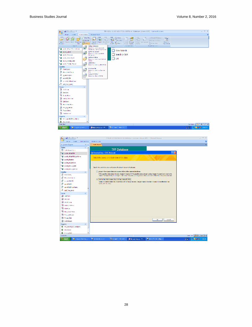
Setting up the Open Database Connectivity on the Client PCs
Once, we had all the tables in the database on the server. The next thing we did was to
modify the Access database on the client laptops. We downloaded the ODBC (Open Database
Connectivity) driver on each of the laptops and set up the ODBC to connect to the database on
the server. Once, the ODBC connection was established, we ran the Microsoft database
application and linked to the tables on the server. All the tables were no longer local but actually
were linked to those tables on the server. Since the tables were on the server, they were
supported in a multiuser environment. This meant multiple users could access the tables,
manipulate, update, and operate at the same time. This greatly enhanced the operation of the
database application. Highlights on the multiuser set up were presented in the Appendix B.
There, we displayed the basic set up of a multiuser client-server database application. Appendix
B includes the screen captures of the following:
Business Studies Journal Volume 8, Number 2, 2016
18
Set up ODBC (Open Database Connectivity) on a client PC;
Add system DSN and configure it;
Connect from MS Access to database on a server via ODBC;
Set Machine Data Source and select a database.
Current Implementation and Usage of the Database Application
At the presence, we are still using the system. In particular, during July, when the local
food pantry is set up to recertify its clients, we would come in and set up four laptop stations to
handle four clients separately but concurrently. If the client is an existing client, then all we need
to do is to pull their record up from the database, update the information, and print out the
application. If the client is the first-time applicant, then we would enter his/her information into
the database and print out the application. Over the years, most of the clients were already in the
database; hence, the recertification process has gone very smoothly with the use of the multiuser
database application. It has been a big relief because gone are the line that extended outside of
the distribution site, the long wait that the clients had to go through, and the stress that the staff
had to face in the manual re-qualifying process.
For months other than July, we set up two laptops with the database applications. One is
used for entering new client information and the other is for viewing and printing existing
clients. At the end of the month, we would come on site and gather these databases and merge
them for use in the next month. We also run reports for the local food pantry and generate the list
of households for sign in. Prior to the computer database, each client had to write his/her
household information including name, gender, number of people in the household, and sign.
Now, we provide the list and the client just looks for his/her name in alphabetical order and then
sign at the designated space next to their name. The process is much more efficient. At the end of
the month, the office manager also uses the information on the list to tabulate how many people
had been served breaking down by gender, race, age, etc.
DISCUSSION
Although teaching the technical skills required of Information Systems (IS) graduates is a
straightforward process, it is far more difficult to prepare students in a normal classroom
environment for the challenges after they graduate and start working in a real world context (Hall
and Johnson, 2012). This is the reason for us to launch the multi-semester project for our
students to work on. As described, the project was based on a real need of the local food pantry.
Students had worked closely with the pantry. They also had to learn the techniques and
methodologies needed to do the project. The emphasis was placed on the application of these
concepts learned in meeting the need of the local food pantry. As a result, students had to follow
systematically the steps involved from doing the analysis to design and development of a
prototype. When the service needed and the course content could be matched, service learning is
appropriate because service performed was a direct application of content and skills learned in
the classroom as shown in this case.
At the end of the two semesters, students were able to finish their required work.
However, while their finished work satisfied the course requirements, it could not fully function
to support the actual operation at the food pantry. The project could have been stopped at this
point, but it did not in this case. A faculty saw this as an opportunity to make contribution and
give back to the community. The faculty led the initiative and had turned the service learning

Business Studies Journal Volume 8, Number 2, 2016
19
project into an academic-community collaboration effort. The goal was to further develop the
prototype into a fully functional database application for a local food pantry to use. In the paper,
we have recounted the details of the journey from our first response to the need of a local
community organization to the initiating and launching of a service learning project and
eventually to the undertaking of the development and implementation of a fully functional
database for use. From our account, we hope to encourage more educators to take on the
opportunities such as service learning projects and academic-community collaboration work.
Although they require time, effort, and extra work, they are meaningful to everyone who involve.
We have learned much from this journey and would like to offer our reflection on what all these
mean to us.
CONCLUSION
Technology constantly advances at an amazing rate. As new technology emerges, it also
brings upon new capabilities. This is particularly evident in the area of information technology
(IT). As we all have seen, the landscape of computer has moved from PC to laptop, to netbook,
then tablets, smartphone, and now wearable gadgets in a relatively short span of time. The good
news is that despite all these changes, technology nowadays is becoming smaller, faster, more
prevalent and powerful, but most importantly it is much more affordable to everyday users. As
we look around, it is hard not to notice that advance in IT has been the key driver for so many
changes in our life and at work. This is why in a typical IS class; we tend to focus much attention
on the newest and latest technology and its impacts. We would spend time to study and analyze
cases where trends such as cloud computing, mobile platform, virtualization, artificial
intelligence, and social media technology help shape our businesses. We try to demonstrate the
power of IT by showing our students how systems like transaction processing systems (TPS),
management information systems (MIS), decision support systems (DSS), and even executive
information systems (ESS) have been used by successful businesses such as Walmart, Bank of
America, GM, etc. Ironically, we tend to neglect those who are not at the bleeding edge. The
question that we should ask ourselves is “What about those small local non-profit
organizations?” These organizations are often underfunded and neglected in terms of using
technology. In the context of the digital divide, these organizations represent the ones being left
behind the technology trend.
Looking at the technology from the digital divide perspective helps us to become more
balanced and sensitive to needs of those have-nots. Indeed, there are many of such have-not
organizations like the local food pantry in this paper who are in desperate need of assistance.
They provide real services to the needy in the community, but at the same time they also need a
lot of help. There are many ways to map and match the resources in the community to the local
needs. Service learning projects and academic-community collaboration effort are two of the
examples where the local resources can be mapped and matched with the needs in a local
community. More importantly, these works are now counted and valued as indicated in the
guideline and expectation set forward by the accreditation bodies such as AACSB and SACS .
In recent years, both AACSB and SACS have emphasized on relevance and impact in
higher education. A journey from a service learning project to an academic community
collaboration effort such as the one described here is based on real world setting. It involves
experiential learning in which students as well as faculties have opportunities to learn, apply, and
practice in a setting authentic to their discipline. Such an initiative could offer a practical
approach to address and meet the requirements for relevance and impact as recommended by the
Business Studies Journal Volume 8, Number 2, 2016
20
higher education accreditation bodies. Moreover, it could serve as an effective pedagogical
approach that connects academic course work with real-world experiences. Series of extensive
activities could be designed and integrated so that students could see the relevance in their
learning and apply their knowledge appropriately in an authentic setting, and at the same time
make a positive impact on a community.
REFLECTION
It is such a refreshing experience and a great opportunity for students, faculty, as well as
a local organization to engage in a carefully match up service learning projects and academic-
community collaboration work. As described in this paper, this is one of the most rewarding and
meaningful ways for those participants to demonstrate the power and relevance of IT in a
classroom setting and at the same time to meet a real need of a local community. First of all, for
students, they learned about the system analysis and design. They understood the concepts in
database design and development. The service learning project provided a real world context in
which they had the opportunity to apply their knowledge and skills. This connection is crucial in
bringing the real world relevance to the classroom learning. Secondly, the faculty members were
able to teach their subject in a meaningful way. They not only taught just IT related concepts but
also exposed their students to the real world needs and gave them the opportunity to give back to
the community. Going beyond the service learning project, the faculty member himself engaged
in a more advanced level through the academic-community collaboration. He took on the role of
a practitioner as he played the leading role in the collaboration effort. The work made real
contribution and created positive impacts in the community. Such academic-community
collaboration was equivalent to a professional development where he could learn new skills,
apply his expertise, share his knowledge with students, and contribute his work to the needs of a
community. The experience helped enriching classroom teaching and stimulate student learning.
At the same time, the faculty was also practicing what he teaches. He was in their field where he
could actually help solving a problem or meeting a need of a local community. Essentially, it was
a unique opportunity for him to serve and to give back to the community. Although this required
time and commitment, at the end, the reward was a feeling of accomplishment for doing
something valuable, meaningful, and making a positive impact on a local community. Finally,
for the local community such as the food pantry in this case, they had their needs met. As a result
of the collaboration with students and faculty member, they received a fully functional database
application. Their work could be done much more efficient and accurate with the computer-
based system. At the end, they could focus more on fulfilling their mission -- That is “to alleviate
hunger for the people and families that it serves throughout the local Parish”. Indeed, this
initiative created a win-win situation for all who had involved in the work.
REFERENCES
Andrews, C, (2007). Service-learning: Applications and Research in Business. Journal of Education for Business,
19-26.
Astin, A. W., & Sax, L. J. (1998). How undergraduates are affected by service participation. Journal of College
Student Development, 39(3), 251-263.
Berson, J. S., & W. F. Younkin. (1998). Doing well by doing good: A study of the effects of a service-learning
experience on student success. In American Society of Higher Education. Miami, FL.
Chuang, K. W. C., & Chen, K. C. (2013). Designing service learning project in systems analysis and design course.
Academy of Educational Leadership Journal. 17(2), 47-60.

Business Studies Journal Volume 8, Number 2, 2016
21
Furco, Andrew. (1996). Service-Learning: A Balanced Approach to Experiential Education. Expanding Boundaries:
Service and Learning. Washington DC: Corporation for National Service, 2-6.
Govekar, M. A., & Meenakshi R. (2007). Service learning: Bringing real-world education into the B-school
classroom. Journal of Education for Business, 83(1), 3-10.
Hall, L. and Johnson, R. (2012). Chapter 7 Preparing IS Students for Real World Interaction with End Users
Through Service Learning: A Proposed Organizational Mode," in Innovative strategies and approaches for
end user computing advancements , edited by Ashish Dwivedi and Steve Clarke, IGI Global, 356 pages
Hillier, A. and Koppisch, D. (2005). Community activists and university researchers collaborating for affordable
housing: Dual perspectives on the experience. Journal of Poverty, 9(4), 27–48.
Hoxmeier, J. & Lenk, M. M. (2003). Service-learning in Information Systems courses: Community Projects That
Make a Difference. Journal of Information Systems Education, 14(1), 91-100.
Huynh, Minh; Chitrakar, Nilesh, Kwok, Ron (2012). Strategy for Academic-Community Collaboration: Enabled and
Supported by the Development of an Open-Source Web Service. PACIS 2012 Proceedings. Pager 18.
Kretzmann, J.P. and McKnight, J.L. (1997). Building Communities from the Inside Out: A PathToward Finding and
Mobilizing a Community's Assets. ACTA Publications, Illinois.
Lennett, J. and Colton, M. E. (1999). A winning alliance: Collaboration of advocates and researchers on the
Massachusetts Mothers Survey. Violence Against Women, 5(10), 1118–1139.
Petkova, O. (2012). Reflections on service-learning projects in Information Systems project management and
implementation course. In Information Systems Educators Conference. New Orleans, LA.
Peterson, D., Minkler, M., Vásquez, V.B. and Baden, A.C. (2006). Community-based participatory research as a
tool for policy change: A case study of the Southern California Environmental Justice Collaborative.
Review of Policy Research, 23(2), 339–353.
Porter, M.E. and Millar, V.E. (1985). How information gives you competitive advantage. Harvard Business Review,
63(4), 149-174.
Real-World Ready QEP Southeastern Louisiana University. (2015, February 2). Retrieved from
http://www.southeastern.edu/resources/qep/QEPSoutheastern.pdf
Reiser, S. L., and Bruce, R. F., Service Learning Meets Mobile Computing, ACM Southeast Regional Conference
2008, 344-350.
Rhoads, R. A. (1998). Academic service-learning: A counternormative pedagogy. In Academic Service Learning: A
Pedagogy of Action and Reflection, edited by Robert A. Rhoads and Jeffrey P. F. Howard. San Francisco:
Jossey-Bass
Ross, L.F., Loup, A., Nelson R.M., Botkin J.R., Kost R., Smith G.R., Gehlert S. (2010). The challenges of
collaboration for academic and community partners in a research partnership: points to consider. Journal of
Empirical Research on Human Research Ethics. 5(1), 19-31.
Tan, J., & Phillips, J. (2005). Incorporating service learning into Computer Science courses. Journal of the
Consortium for Computing Sciences in Colleges, 20(4), 57-62.
Toncar, M. F., Reid, J. S., Burns, D. J., Anderson, C. E., & Nguyen, H. P. (2006). Uniform assessment of the
benefits of service learning: The development, evaluation, and implementation of the Seleb Scale. Journal
of Marketing Theory and Practice, 14(3), 223-38.
Viswanathan, M., Ammerman, A., Eng, E., Gartlehner, G., Lohr, K.N., Griffith, D., Rhodes, S.,Samuel-Hodge, C.,
Maty, S., Lux, L., Webb, L., Sutton, S. F., Swinson, T., Jackman, A. and Whitener, L. (2004). Community-
Based Participatory Research: Assessing the Evidence. Evidence Report/Technology Assessment No. 99
(prepared by RTI University of North Carolina Evidence-Based Practice Center under Contract No. 290–
02–0016), AHRQ Publication 04-E022–2, Rockville, MD, Agency for Healthcare Research and Quality.
Weis, W. L. (2000). Service-learning in Business curricula: Walking the talk. National Society for Experiential
Education Quarterly, 11-16.

Business Studies Journal Volume 8, Number 2, 2016
22
APPENDIX A
The following figures provide the core elements in the database application including: the
Entity-Relationship Diagram, the interface of the input form, samples of the application and
report, examples of codes and queries.
Figure A1
ENTITY-RELATIONSHIP DIAGRAM FOR THE LOCAL FOOD PANTRY DATABASE

Business Studies Journal Volume 8, Number 2, 2016
23
Figure A2
THE INTERFACE OF THE INPUT FORM

Business Studies Journal Volume 8, Number 2, 2016
24
Figure A3
A PRINT-OUT SAMPLE OF THE APPLICATION
Figure A4
A SAMPLE OF A REPORT
Figure A5
EXAMPLE OF VISUAL BASIC CODES

Business Studies Journal Volume 8, Number 2, 2016
25
Figure A6
EXAMPLE OF QUERIES

Business Studies Journal Volume 8, Number 2, 2016
26
APPENDIX B
The following figures illustrate how to set up the ODBC to allow connection from
Microsoft Access to the database on the server.
Figure B1
SET UP ODBC ON THE CLIENT PC

Business Studies Journal Volume 8, Number 2, 2016
27
Figure B2
ADD SYSTEM DSN AND CONFIGURE IT
Figure B3
CONNECT FROM MS ACCESS TO DATABASE ON THE SERVER VIA ODBC
Business Studies Journal Volume 8, Number 2, 2016
28

Business Studies Journal Volume 8, Number 2, 2016
29
Figure B4
TAB MACHINE DATA SOURCE AND SELECT THE DATABASE

Business Studies Journal Volume 8, Number 2, 2016
30
DOES TRANSFORMATION LEADERSHIP PROMOTE
INNOVATION PRACTICES IN E-COMMERCE?
Dr. Joe Ilsever, University of the Fraser Valley
Omar Ilsever, Our Lady of the Lake University
ABSTRACT
Organizations face many challenges in today’s dynamic business environment
(Gumusluoglu & Ilsev, 2009). Rapid technological changes, shortened product life cycles and
globalization have made it necessary for organizations to be more creative and innovative to
survive, compete, grow and lead (Gumusluoglu & Ilsev, 2009). Therefore, innovation is a key
factor in organizations’ ability to create a sustainable competitive advantage as well as for the
success of strong economies in the 21st century (Eisenbeiss, Boerner & Knippenberg, 2008).
Evidently, it has been suggested that leadership is among the most important factors affecting
innovation (Gumusluoglu & Ilsev, 2009). A number of studies have shown that transformational
leadership positively influences organizational innovation (Gumusluoglu & Ilsev, 2009).
However, limited studies have discussed how other leadership styles such as transactional and
laissez-faire leadership may be utilized and may be more beneficial for organizations to adapt
for innovative practices. Without such initiatives, companies could fall into product dormancy
and loss of market share.
INTRODUCTION
This paper will critically assess the three leadership styles and determine if
transformational leadership does indeed promote innovation practices or if other leadership
styles such as transactional leaders or laissez faire leaders would be more beneficial for
organizations to implement, for future success in innovation. In the following sections, a critical
assessment of both transformational and transactional leadership, as well as laissez faire
leadership will be conducted. The last section will determine which style would be more
appropriate for organizations to adapt and whether transformational leadership is a better fit for
innovation.
CRITICAL REVIEW: TRANSFORMATIONAL LEADERSHIP ON
ORGANIZATIONAL INNOVATION
Transformational leadership defined by Gumusluoglu & Ilsev (2009) are leaders who
“transform followers” personal values and self-concepts, move them to higher levels of needs
and aspirations and raise the performance expectations of their followers.” This leadership style
has four main components: idealized influence, inspirational motivation, intellectual stimulation,
and individualized consideration (Bass, Jung, Avolio & Berson, 2003). Tichy & Devanna (1990)
highlight the transforming effect these leaders can have on organizations as well as on
individuals. By defining the need for change, creating new visions and mobilizing commitment
to these visions, leaders can ultimately transform the organization (Ticky & Devanna, 1990).
Gumusluoglu & Ilsev (2009) further state that transformational leadership is an important
determinant of organizational innovation and should be implemented by managers to promote

Business Studies Journal Volume 8, Number 2, 2016
31
strong innovation practices in organizations. Those in favor of transformational leadership in
organizations argue that these types of leaders effectively increase commitment from employees
and elevate higher level needs such as self-actualization and self-esteem (Bass, 1990). As a
result, employees are highly motivated, which can be an important driver of both employee
creativity and firm innovation (Gumusluoglu & Ilsev, 2009). Essentially, transformational
leaders encourage their employees to identify new approaches to problem solving as well as
looking at old problems in new ways (Gumusluoglu & Ilsev, 2009). Under these positive
environments, employees are more likely to be engaged in innovative ideas (Oke, Munshi, &
Walumbwa, 2009). Overall, researchers tend to agree on the role of transformational leadership
of top management in enhancing quality management (Berson & Linton, 2005). However, there
is little agreement regarding the role of transformational leadership at lower levels of the
organization (Berson & Linton, 2005). For example, Dean and Bowen (1994) suggest that
quality management practices could be seen as substitutes to leadership. In other words,
instituting effective quality management practices diminishes the need for transformational
leadership at lower levels of a firm (Sousa and Voss, 2002).
TRANSACTIONAL LEADERSHIP ON ORGANIZATION INNOVATION
Transactional leadership is the style of leadership that is most often seen in businesses
and organizations today (Humphreys, 2001). Transactional leadership is usually characterized by
the factors of “contingent reward and management-by-exception” (Bass, 1990). The key to
transactional leadership is the exchange between the leader and the follower (Humphreys, 2001).
They influence each other in ways that both receive something of value. They are said to be
mutually dependent upon one another (Humphreys, 2001). Transactional leadership theories are
all founded on the idea that leader-follower relations are based on a series of exchanges or
implicit bargains between leaders and followers (Hartog, Muijen & Koopman, 1997).
Oke et al. 2009 suggest that “transactional leaders are likely to contribute to innovative
processes and activities by clarifying what performance standards are required and how needs
would be satisfied.” Essentially, transactional leaders contribute to the innovation process by
encouraging people to perform in a desired way by motivating them through rewards and
punishment (Gumusluoglu & Ilsev, 2009). The transactional leader has clear performance
expectations, goals, and paths that link achievement of the goals to rewards (Hartog et al, 1997).
However, Bass et. al (2003) & Humphreys (2001) also discuss how a transactional leader
can have a negative impact on organizational innovation if they are constant reprimanding or
disapproving of actions taken by employees. Contingent reprimand has a negative impact on
employee performance, meaning they are less likely to want to achieve the desired result by its
leaders. (Bass et. Al, 2003, Humphreys, 2001.)
LAISSEZ-FAIRE LEADERSHIP ON ORGANIZATIONAL INNOVATION
Both transformational and transactional leaders are active leaders. They actively
intervene and try to prevent problems. When researching these two active forms of leadership,
they are often contrasted with extremely passive laissez-faire leadership (Hartog et al, 1997).
Laissez faire leadership describes passive leaders who are reluctant to influence subordinates or
give direction (Deluga, 1990). They generally refrain from participating in-group or individual
decision-making and to a large extent, abdicate their leadership role (Deluga, 1990).
Subordinates are given considerable freedom of action and, therefore, seem likely to maximize
Business Studies Journal Volume 8, Number 2, 2016
32
their power and influence (Gumusluoglu & Ilsev, 2009). This is a leader who is “relatively
inattentive, indifferent, frequently absent, and un-influential” (Gumusluoglu & Ilsev, 2009). As
stated by Hartog et al, (1997) laissez-faire leadership is an inappropriate way to lead. However,
Hartog et al, (1997) also states, “one could probably define situations in which highly active
leadership is not necessary and may not even be desirable.” For instance, in their substitutes for
leadership theory Kerr & Jermier (1978) propose several subordinate, task, and, organization
characteristics that could reduce the importance of leadership (Hartog et al, 1997). A less active
role of leaders could also lead to 'empowerment' of followers (Hartog et al, 2007). However, in
the long run this type of leadership would not be beneficial. Thus, this leadership style is
ineffective in organizations that are wanting to be innovative in their ideas and approaches. In
addition, laissez-faire leadership has shown strong negative relationships with various leadership
criteria (Hinkin & Schriesheim, 2008).
TRANSFORMATIONAL, TRANSACTIONAL, LAISSEZ-FAIRE LEADERSHIP:
WHAT LEADERSHIP STYLE WORKS?
Although transformational and transactional leadership are distinct leadership styles,
contrasting transactional and transformational leadership does not imply that the models are
unrelated (Hartog et al, 1997). Burns (1978) thought of the two types of leadership as being at
opposite ends of a continuum (Hartog et al, 1997). Bass (1985) however viewed them as separate
dimensions, this means a leader can be both transactional and transformational (Hartog et al,
1997). In fact, both are necessary for organizational performance, and the best leaders are both
transformational and transactional (Oke et. al 2009). However as both work in different ways to
motivate employees, and neither are substitutable, Bass et al (2003) suggest that transformational
leadership is more likely to reflect social values and to emerge in times of distress and change
while transactional leadership are more likely to be observed in a well-ordered society.
Hartog et al. (1997) states that while transactional leadership motivates subordinates to
perform as expected, the transformational leader typically inspires followers to do more than
originally expected (Hartog et al, 1997). Bass (1990) further argues that the leadership
continuum ranges from complete non-leadership, which he believes to be laissez-faire at one
extreme end to the very active leader, which he views as transformational leadership. Other
transformational leadership theorists (e.g., Burns, 1978; Bass, 1985; Bass and Avolio, 1994)
have argued the same, stating that leadership styles can be placed on a continuum in terms of
leader pro-activity and effectiveness (Berson & Linton, 2005). At the bottom end of this
continuum or range is laissez-faire leadership (Berson & Linton, 2005). In the middle range is
transactional leadership behavior and at the top is transformational (Berson & Linton, 2005).
This range implies that transformational leadership is more proactive and ultimately more
effective than transactional and laissez faire leadership in terms of motivating followers to
achieve higher performance (Berson & Linton, 2005).
Organizational innovation in Gumusluoglu & Ilsev (2009) study is defined as the
“tendency of the organization to develop new or improved products and services and its success
in bringing those products and services to the market.” Therefore, leaders must display attributes
that promote innovation and innovation practices in order to be both successful in product
development and marketing. Overall, transactional leaders tend to get results by thinking more
about specific goals, work skills, work assignments and various reward relationships and offering
reward relationships to employees (Oke et. al 2009). Alternatively, transformational leaders

Business Studies Journal Volume 8, Number 2, 2016
33
place greater emphasis upon intellectual capability and creativity by providing the emotional
support that encourages employees to excel (Oke et. al 2009).
Furthermore, Oke et al. (2009) suggest that the “transactional form of leadership, through
its focus on management, clear structures, formal systems, reward and discipline is likely to be
more effective in the implementation stage of innovation than transformational leadership.”
Transformational leadership style is more appropriate to foster the creative innovation process
than the transactional leadership style, since the creative endeavor requires risk-taking,
experimentation, change and challenges to the status quo (Oke et al, 2009).
In regards to laissez-faire leadership, subordinates compete for the power and influence
abdicated by the laissez faire leader, meaning there is a lack of leadership, resentment, intense
competition and manipulation between employees and management, which in turn does not
foster innovation practices or growth, especially for organizations in today’s technology driven
work environment (Deluga, 1990). Therefore, organizations that want to be successful in
innovation implementation must consider alternate leadership styles such as transformational
leadership to have a positive influence and strong impact on organizational innovation
(Gumusluoglu & Ilsev, 2009).
IS TRANSFORMATIONLAL LEADERSHIP A BETTER FIT FOR INNOVATION?
Humphreys (2001), states that there is little question that advancing technologies will
impact the traditional view of leadership and that emerging technologies will have greater
implications on effective leadership behaviors and leadership paradigms. Therefore, it makes
sense that organizations should implement transformational leaders, as they promote innovation
practices and utilize the most appropriate leadership qualities for this day and age; where
continual change is driven by escalating technological advancement (Humphreys, 2001).
Furthermore, Bass (1990) indicates that transformational leadership can lead to substantial
organizational rewards. Transformational leadership has also been positively correlated to leader
effectiveness ratings, leader and follower satisfaction, follower efforts, and overall organizational
performance (Humphreys, 2008).
Transformational leadership is evidently the better leadership style that enhances
innovation within an organization. Using charisma, transformational leaders instill admiration,
respect, and loyalty and emphasize a sense of mission (Gumusluoglu & Ilsev, 2009). They also
build a one-to-one relationship with his or her followers and understand their individual needs,
skills and aspirations (Gumusluoglu & Ilsev, 2009). Thus, transformational leaders meet the
emotional needs of each employee (Bass, 1990). By inspirational motivation, the leader
articulates an exciting vision of the future, shows the followers the ways to achieve the goals,
and expresses his or her belief that they can do it (Gumusluoglu & Ilsev, 2009). In addition to its
effect on the tendency of organizations to innovate, transformational leadership also has a
positive impact on the market success of the innovations (Gumusluoglu & Ilsev, 2009). By
articulating a strong vision of innovation and displaying a sense of power and confidence, this
leader will strive to ensure the market success of the innovation (Gumusluoglu & Ilsev, 2009)
Furthermore, in addition to the internal roles, transformational leadership has been suggested to
be effective in playing external roles such as boundary spanning, entrepreneuring and
championing, which might be important both for understanding the needs of the market and
marketing the innovation successfully (Gumusluoglu & Ilsev, 2009).

Business Studies Journal Volume 8, Number 2, 2016
34
CONCLUSION
To remain competitive in today’s rapidly changing work environment, organizations
must continually develop leaders who will support innovation and emerging technology
(Humphreys, 2001). Transformational leaders promote higher performance in organizational
units that are open to change and are flexible, in other words, in an innovative climate
(Gumusluoglu & Ilsev, 2009). Therefore, transformational leadership is ideal in organizations
that want to innovate successfully. Transformational leaders do not settle for current states but
articulate an appealing and challenging future vision (Eisenbeiss et al, 2008). Transformational
leaders also display unconventional and creative behavior and serve as role models for
innovation (Eisenbeiss et al, 2008). Overall, transactional and laissez-faire leadership do not
articulate the qualities needed for a good leader in innovative organizations. Although a
transactional leader may be useful in the implementation stage of innovation, it is apparent that
the transformational leader’s style is more catered to that of innovation. Additionally, for
organizations to be successful in their innovation practices, strong and dedicated leadership is
key, therefore laissez faire leadership would not be acceptable in innovative organizations.
Transformational leaders promote innovative practices and are essential in organizational
innovation (Gumusluoglu & Ilsev, 2009). Therefore, the presence of transformational leaders
will strongly assist in an organizations ability to successfully innovate in today’s changing
business environment.
REFERENCES
Avolio, B.J., Bass, B.M. (1993). Transformational Leadership and Organizational Culture. Public Administration
Quarterly, 17(1), 112-121.
Balsano, T., Goodrich, N., Lee, R., Miley, J., Morse, T., & Roberts, D. (2008, November). Identify Your Innovation
Enablers And Inhibitors. Research Technology Management, 51(6), 23-33.
Bureaucracy. (2001). Dictionary of Human Resource Management, Retrieved June 14, 2009, from Business Source
Premier database.
Cohn, J., Katzenbach, J., & Vlak, G. (2008). Finding and Grooming Breakthrough Innovators. Harvard Business
Review, 86(12), 62-69.
De Cremer, D. (2006). Affective and motivational consequences of leader self-sacrifice: The moderating effect of
autocratic leadership. The Leadership Quarterly,17,79-93.
Educating Innovative Leaders: Lessons in Processes and Performance. (2006). Chief Learning Officer, Retrieved
June 8, 2009, from Business Source Premier database.
Gabris, G., Grenell, K., Ihrke, D., & Kaatz, J. (1999). Managerial innovation as affected by administrative
leadership and policy boards. Public Administration Quarterly, 23(2), 223-249.
Gronn, P. (1999). A realist view of leadership. Paper presented at the educational leaders for the new millenium-
leaders with soul. ELO-AusAsia. On-line Conference.
Hartog, D., Van Muijen, J., & Koopman, P. (1997). Transactional versus transformational leadership: An analysis of the MLQ. Journal of Occupational & Organizational Psychology, 70(1), 19-34.
Jenssen, J., & Jørgensen, G. (2004). How Do Corporate Champions Promote Innovations? International Journal of
Innovation Management, 8(1), 63-86.
Minett, D., Yaman, H. R., Denizci, B. (2009). Leadership styles and ethical decision making in hospitality
management. International Journal of Hospitality Management.
Oke, A., Munshi, N., & Walumbwa, F. (2009). The Influence of Leadership on Innovation Processes and Activities.
Organizational Dynamics, 38(1), 64-72.
Topalian, A. (2000). The Role of Innovation Leaders in Developing Long-Term Products. International Journal of
Innovation Management, 4(2), 149.

Business Studies Journal Volume 8, Number 2, 2016
35
Vecchio, R., Justin, J., & Pearce, C. (2008). The utility of transactional and transformational leadership for
predicting performance and satisfaction within a path-goal theory framework. Journal of Occupational &
Organizational Psychology, 81(1), 71-82.
Weber, M. (1947). The Theory of Social and Economic Organization. Translated by A.M. Henderson & Talcott
Parsons, The Free Press.

Business Studies Journal Volume 8, Number 2, 2016
36
IMPLIED VERSUS REALIZED VOLATILITY OF S&P
500: EFFECTS OF STOCK MARKET FACTORS
Andrey Kudryavtsev, The Max Stern Yezreel Valley Academic College
ABSTRACT
This study analyzes the ability of the implied volatility index (VIX) to incorporate
available contemporary stock market information, which is relevant for the volatility forecasts.
Employing a number of market factors positively correlated with actual future market volatility,
namely, historical (past) market volatility, general stock market trading volume and significant
stock market returns, it documents that VIX is positively correlated with them, but on the other
hand, does not manage to account for them fully and immediately, or in other words, under-
reacts to relevant market information. One of the possible explanations for this finding may be
that investors' tend to be "anchored" towards (or over-affected by) the recent implied volatility
measures, causing VIX to be relatively sticky and relatively less affected by relevant market
factors, compared to the realized future volatility.
Keywords: Anchoring; Historical Volatility; Implied Volatility; Under-Reaction;
Volatility Forecasts; VIX.
JEL Classification Codes: D80, D84, G12, G14, G17.
INTRODUCTION
Volatility is a fundamental characteristic of financial markets. Although a derived
number, describing the propensity of prices to fluctuate, it plays an important role in options
pricing and in any simple characterization of market dynamics. Therefore, much effort has been
invested in forecasting stock market volatility. The two sources of information most widely
employed in future volatility forecasts are the historical (realized) volatility measures and
implied volatility measures.
The most commonly used measure of implied volatility is the Volatility Index (VIX)
introduced by Whaley (1993) and launched by the Chicago Board Options Exchange (CBOE) in
1993. VIX is based on the prices of S&P 500 index options, providing thereby a benchmark for
the expected future market volatility over the next month. The index is calculated in real-time
and is continuously disseminated throughout each trading day. VIX is widely followed and has
been cited in hundreds of news articles in leading financial publications. Since VIX represents an
implied measure of expected future volatility, it has been labeled the investors’ 'fear gauge' (see
Whaley, 2000; 2008). According to this interpretation, though there are other factors affecting
this index, in most cases, high VIX reflects increased investors' fear and low VIX suggests
complacency. Whaley (2008) documents negative correlation between daily S&P 500 index
returns and VIX changes, and interprets it as indicating that changes in the VIX are partially
driven by investors demanding portfolio insurance in times of high current market volatility.
The previous financial literature tends to conclude that implied volatility measures tend to
outperform realized volatility measures in forecasting future volatility. Latane and Rendleman
(1976), Chiras and Manaster (1978), and Beckers (1981) provide early assessments of implied
volatility forecast quality. They find that implied volatilities offer better estimates of future
Business Studies Journal Volume 8, Number 2, 2016
37
return volatility than ex-post standard deviations calculated from historical returns data. More
recently, Jorion (1995) finds that implied volatilities from currency options outperform volatility
forecasts from historical price data. Christensen and Prabhala (1998), Christensen and Strunk-
Hansen (2002), and Fleming (1998) find that implied volatility forecasts dominate historical
volatility in terms of ex-ante forecasting power. Blair, Poon and Taylor (2001) show that
historical prices (even intraday prices) do not provide much incremental information compared
to the information given by VIX; moreover, VIX provides the best out-of-sample forecasts of
realized volatility. Jiang and Tian (2005) deem the information content of the VIX volatility
forecast superior to alternative implied volatility measures as well as forecasts based on
historical volatility.
Another related issue discussed in the previous literature is the "absolute" accuracy of
implied volatility measures in predicting future stock market volatility. Chernov (2001) notes
that implied volatilities are generally higher than realized ones. Christensen and Prabhala (1998),
Christensen and Strunk-Hansen (2002) and Fleming (1998) document that implied volatility
forecasts are upwardly biased. Carr and Wu (2009) and Bollerslev, Tauchen and Zhou (2009)
conclude that typically the spot VIX computed from option prices embeds volatility risk
premium and exceeds realized volatility.
Yet, a question that has not been raised in the previous literature is whether implied
volatility measures, and VIX, in particular, fully and immediately incorporate current stock
market information that is relevant for volatility forecasts. The present study makes an attempt to
fill this gap by examining effect of historical market volatility, market trading volume and
significant stock market returns on the ratio of VIX and the subsequently realized market
volatility. In this context, it documents that VIX, though correctly reacts to these relevant factors,
does not manage to fully forecast their effects on future market volatility. This kind of under-
reaction demonstrated by VIX may be possibly attributed to investors' general tendency to be
"anchored"1 towards current variable or index values, which may cause the expectations with
respect to a given variable or index to be relatively sticky and not to account completely for all
relevant information.
The rest of the paper is structured as follows: Section 2 describes the data sample and the
volatility estimation procedure. Section 3 comprises the research hypothesis and the results.
Section 4 concludes.
DATA DESCRIPTION AND VOLATILITY ESTIMATES
The present research employs the daily quotes of VIX and S&P 500 (the underlying
index) for the period from January 1990 to December 2012 (overall, 5,797 trading days)
extracted from www.finance.yahoo.com. For the sampling period, the daily log close-to-close
returns on S&P 500 are calculated.
For every 22 consecutive trading days, roughly representing one trading month, the
volatility of S&P 500 returns is calculated as a standard deviation of daily returns. In order to
make the resulting figures commensurable with the VIX quotes, denoting the one-month-ahead
implied volatility of S&P 500 expressed in percent and in yearly terms, they are multiplied by
100 and then by 202. To summarize, for every 22 consecutive trading days, the realized monthly
market volatility is calculated as:

Business Studies Journal Volume 8, Number 2, 2016
38
20*100*22
)(22
1
2
22,1
22,1
t
t rr
V (1)
where: tr is the S&P 500 log return on day t; and 22,1r is the average S&P 500 daily return over
days 1 to 22.3
In this way, for each trading day t, it is possible to define the last month's (past or
historical) volatility ( tPV ) and the next month's (future) volatility ( tFV ) as:
1,22 ttt VPV and 22,1 ttt VFV (2)
Table 1 reports the basic descriptive statistics over the sampling period of VIX quotes, of
the subsequently realized actual market volatility, calculated according to formula (2), and of the
ratio of the two, calculated for each trading day t as:
t
t
tFV
VIXVR (3)
where: tVR represents the implied-to-realized Volatility Ratio.
Table 1
DESCRIPTIVE STATISTICS OF THE IMPLIED AND THE REALIZED MARKET VOLATILITY
MEASURES AND THEIR RATIO
Statistics Implied and realized volatility measures
VIX Realized Volatility
(FV)
Volatility Ratio (VR)
Mean
Median
Standard Deviation
Maximum
Minimum
20.45
18.88
8.13
80.86
9.31
20.23
17.32
12.09
110.95
5.97
1.12
1.08
0.32
2.76
0.26
The Table shows that, though the mean VIX and FV measures are quite close to each
other (20.45 and 20.23, respectively), VIX, ranging from 9.31 to 80.86 with a standard deviation
of 8.13, is less volatile than the subsequently realized market volatility, ranging from 5.97 to
110.95 with a standard deviation of 12.09. The volatility ratio has a relatively low standard
deviation of 0.32, indicating that contemporaneous VIX and FV measures tend not to deviate too
much from each other, or in other words, that VIX represents a reasonable forecast of one-
month-ahead market volatility.
In order to verify the latter inference, Table 2 presents the results of a simple regression
model predicting the next month's market volatility based on the current value of VIX, namely:
ttt VIXFV 10 (4)
where: tVIX represents the day-t closing value of VIX.

Business Studies Journal Volume 8, Number 2, 2016
39
Table 2
THE PREDICTIVE ABILITY OF VIX WITH RESPECT TO THE SUBSEQUENTLY REALIZED
ACTUAL MARKET VOLATILITY (DEPENDENT VARIABLE – FV)
Explanatory variables Regression coefficients (t-statistics)
Intercept
VIX
***-3.227 (-11.79)
***1.147 (92.21)
Adjusted R-Squared 0.595 Asterisks denote 2-tailed p-values: ***p<0.01
As it might be expected, the coefficient estimate for tVIX is positive (1.147) and highly
significant. The adjusted R-squared of this simple regression model is also impressively high
(0.595), demonstrating that, consistently with the previous literature, VIX represents a high-
quality forecast of the future market volatility.
RESEARCH HYPOTHESIS AND RESULTS
The previous Section's results confirm that VIX represents a good forecast of the future
stock market volatility. But is VIX able to fully and immediately incorporate current stock
market information that is relevant for the volatility forecasts? The major goal of this study is to
answer this question. In this respect, I hypothesize that investors, when forming their estimates
of the "correct" contemporaneous implied volatility, should be probably over-affected by recent
implied volatility measures, causing VIX to be relatively sticky and under-react to relevant
information.
In this context, first of all (in Subsection 3.1) three contemporaneous market factors that
are highly correlated with the realized future market volatility are established, and furthermore
(in Subsection 3.2) a test for their effects on VIX and on the ratio of VIX and the subsequently
realized market volatility is carried.
Market factors correlated with future market volatility
Stock market volatility may be affected by a very wide range of market factors. The
present study concentrates on three of them, with the final goal of testing if VIX is able to fully
and immediately reflect them, or in other words, if these factors systematically affect the ratio of
VIX and the subsequently realized market volatility. These factors include:
Past (Historical) Market Volatility
The previous literature dealing with stock volatility clearly indicates that market volatility
over different periods of time is positively autocorrelated and that past volatility may serve a
good (though slightly worse than implied volatility) forecast of future volatility (e.g., Fleming,
1998; Blair et al., 2001; Jiang & Tian, 2005). Therefore, the realized future market volatility
( tFV ) may be expected to be positively correlated with the respective past market volatility
( tPV ).
Market Trading Volume
Trading volume activity, in general, is recognized to be a reflection of heterogeneous
investors’ expectations (e.g., Copeland, 1976; Pfleiderer, 1984; Varian, 1985). Karpoff (1986)

Business Studies Journal Volume 8, Number 2, 2016
40
demonstrates that trading volume has essentially two causes – dispersion in prior expectations
and idiosyncratic interpretations of information events. He also shows that the increase in trading
volume is positively correlated with the information “surprise”. On the other hand, the new
incoming information is also one of the major causes of stock price volatility. Thus, an increased
trading volume in a stock market is usually a result of an increased flow of information and may
serve a hint for increased subsequent market volatility. For each trading day t in the sampling
period, the abnormal market trading volume ( tAVol ), with respect to the previous trading month,
is calculated as:
):(
):(
122
122
tt
ttt
tVolVolStDev
VolVolAverageVolAVol (5)
where: tVol represents the total day-t trading volume in S&P 500 stocks.4
In the light of the aforesaid, tFV may be expected to be positively correlated with tAVol .
Substantial Stock Market Returns
Similarly to the abnormally high daily trading volumes, substantial daily changes (both
rises and falls) in the stock market index may be a result of important information arriving at the
market, and may serve an indication for the increased future market volatility. Similarly to
Fabozzi and Francis (1977) and Kliger and Kudryavtsev (2010), this study defines the days of
substantial changes in S&P 500 as the days when the absolute value of S&P 500 return was
larger than half standard deviation of S&P 500 returns measured over the total sampling period.
The "substantial" dummy variable ( tSDum ) is defined to be equal to 1 for the days with
substantial S&P 500 returns (overall, 2,717 trading days), and 0 for the rest of the sampling
period days (overall, 3,080 trading days). In the light of the aforesaid, tFV may be expected to
be positively correlated with tSDum .
First of all, the effects of the three aforementioned variables' contemporaneous values on
the subsequent month's market volatility are verified. For this purpose, three linear regressions of
the following format are performed:
ttt FactorFV 10 (6)
where: tFactor refers to tPV , tAVol and tSDum , respectively, for each of the three regressions.
Table 3 presents the regressions' results, and most notably the highly significant
coefficient estimates of 0.731, 0.593 and 6.160 for the past market volatility, the abnormal
market trading volume, and the "substantial" dummy, respectively. Thus, as expected, the three
factors are positively correlated with the subsequently realized stock market volatility, and
represent its significant predictors. One more thing to note is that, in line with the previous
literature, the predictive power of VIX with respect to the future volatility, as expressed by the
adjusted R-squared of regression (4) (0.595 – see Table 2) is higher than that of the past volatility
(0.535).

Business Studies Journal Volume 8, Number 2, 2016
41
Table 3
THE EFFECTS OF THREE MARKET FACTORS ON SUBSEQUENT MARKET VOLATILITY
(DEPENDENT VARIABLE – FV)
Explanatory
variables
Regression
coefficients
(t-statistics)
Explanatory
variables
Regression
coefficients
(t-statistics)
Explanatory
variables
Regression
coefficients
(t-statistics)
Intercept
PV
***5.459
(25.69)
***0.731
(81.61)
Intercept
AVol
***20.206
(127.39)
***0.593
(4.66)
Intercept
SDum
***17.342
(82.29)
***6.160
(20.01)
Adjusted
R-Squared
0.535 Adjusted
R-Squared
0.004 Adjusted
R-Squared
0.064
Asterisks denote 2-tailed p-values: ***p<0.01
Reaction of VIX to Market Factors and its Ability to Reflect Them
After establishing positive and significant correlation of the three aforementioned market
factors with the future market volatility, the next step is to verify if VIX, that, according to the
previous literature and the results in Section 2, represents a high-quality forecast of the future
volatility, properly reacts to these factors. Three linear regressions are run, which are similar to
regressions (6), but with VIX instead of FV as a dependent variable, that is:
ttt FactorVIX 10 (7)
Table 4 reports the regressions' results. The coefficient estimates of 0.596, 0.176 and
5.177 for the past market volatility, the abnormal market trading volume, and the "substantial"
dummy, respectively are lower than the respective based on regression (6), but are still highly
significant. So it appears that though VIX is affected by the market factors more weakly than the
future volatility is, it is still positively and significantly correlated with the factors, suggesting
that investors correctly take them into account. Another finding interesting in itself is the
extremely high goodness-of-fit (0.786) of the regression of VIX on PV, indicating that the
realized historical volatility is by far the most important factor affecting implied volatility.
Table 4
THE EFFECTS OF THREE MARKET FACTORS ON VIX (DEPENDENT VARIABLE – VIX)
Explanatory
variables
Regression
coefficients
(t-statistics)
Explanatory
variables
Regression
coefficients
(t-statistics)
Explanatory
variables
Regression
coefficients
(t-statistics)
Intercept
PV
***8.386
(87.03)
***0.596
(145.83)
Intercept
AVol
***20.443
(191.41)
**0.176
(2.05)
Intercept
SDum
***18.023
(129.75)
***5.177
(25.51)
Adjusted
R-Squared
0.786 Adjusted
R-Squared
0.001 Adjusted
R-Squared
0.101
Asterisks denote 2-tailed p-values: **p<0.05; ***p<0.01
Business Studies Journal Volume 8, Number 2, 2016
42
So, by now, the (quite not surprising) results confirm that VIX represents a strong
predictor of the one-month-ahead market volatility and correctly reacts to relevant market
factors. At this stage, however, the study arrives at its main question, namely: "Is VIX able to
fully and immediately incorporate current stock market information that is relevant for the
volatility forecasts?"
In this respect, it may be expected that VIX, though positively correlated with the
relevant market factors, should not be able to account for them fully and immediately, or in other
words, should under-react to relevant information. This expectation is based on the well-
documented people's tendency to form their estimates for different categories, starting from a
particular available, and often irrelevant, value and insufficiently adjusting their final judgments
from this starting value. This tendency represents a simplifying decision-making rule, known as
anchoring (or anchoring bias), and may cause the expectations with respect to a given variable
or index to be relatively sticky and not to account completely for all relevant information. In
other words, it may cause people to be "anchored" towards the current value of the variable or
index.
The term "anchoring" was introduced in one of the most cited ever studies by Tversky
and Kahneman (1974). They argue that in many situations people make estimates by considering
an initial value that they adjust upwards or downwards to yield a final estimate. Such
adjustments are often insufficient, leaving judgments biased in the direction of the initial
"anchor" value. In what is probably the best-known demonstration of this effect, Tversky and
Kahneman (1974) first ask their research participants whether the percentage of African nations
in the United Nations (target number) is higher or lower than an arbitrary number (the anchor)
which is randomly determined by spinning a wheel of fortune (e.g., 65% or 10%). The
participants are then asked to give their best estimate of this percentage. The absolute judgments
are assimilated to the provided anchor value so that the mean estimate of participants who have
received the high anchor is 45%, compared to 25% for participants who have received the low
anchor.
The anchoring effects have proved to be a truly ubiquitous phenomenon that has been
observed in general knowledge questions (e.g., Jacowitz & Kahneman, 1995; Strack &
Mussweiler, 1997; English, 2008), probability assessments (e.g., Plous, 1989; Chapman &
Johnson, 1994), legal judgment (e.g., Markovsky, 1988; Chapman & Bornstein, 1996), and a
number of other fields. There is also a continuously growing body of literature documenting the
effects of anchoring on different aspects of economics and finance, including, for example, real-
estate pricing (Northcraft & Neale, 1987), buyers' and sellers' behavior (Galinsky & Mussweiler,
2001), auctions (Beggs & Graddy, 2009), advertising (Biswas & Burton, 1993), technical
analysis (Zielonka, 2004), and general stock market analysis (Fischer & Statman, 2000;
Kudryavtsev & Cohen, 2010a, 2010b). Gruen and Gizycki (1993) use anchoring to explain the
widely-observed anomaly that forward discounts do not properly explain subsequent exchange
rate movements. They argue that anchoring phenomenon may be relevant to the "sticky prices"
that are so talked about by macroeconomists. So long as past prices are taken as suggestions of
new prices, the new prices will tend to be close to the past prices. The more ambiguous the value
of a commodity, the more important a suggestion is likely to be, and the more important
anchoring is likely to be for price determination.
Adopting the idea by Gruen and Gizycki (1993), this study suggests that investors, when
forming their estimates of the "correct" contemporaneous implied volatility, may be "anchored"
towards the recent implied volatility measures, causing VIX to be relatively sticky and under-
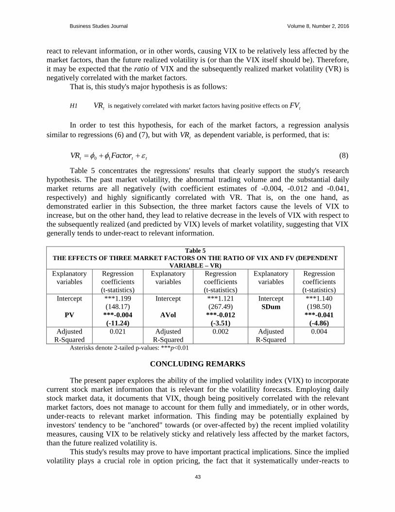
Business Studies Journal Volume 8, Number 2, 2016
43
react to relevant information, or in other words, causing VIX to be relatively less affected by the
market factors, than the future realized volatility is (or than the VIX itself should be). Therefore,
it may be expected that the ratio of VIX and the subsequently realized market volatility (VR) is
negatively correlated with the market factors.
That is, this study's major hypothesis is as follows:
H1 tVR is negatively correlated with market factors having positive effects on tFV
In order to test this hypothesis, for each of the market factors, a regression analysis
similar to regressions (6) and (7), but with tVR as dependent variable, is performed, that is:
ttt FactorVR 10 (8)
Table 5 concentrates the regressions' results that clearly support the study's research
hypothesis. The past market volatility, the abnormal trading volume and the substantial daily
market returns are all negatively (with coefficient estimates of -0.004, -0.012 and -0.041,
respectively) and highly significantly correlated with VR. That is, on the one hand, as
demonstrated earlier in this Subsection, the three market factors cause the levels of VIX to
increase, but on the other hand, they lead to relative decrease in the levels of VIX with respect to
the subsequently realized (and predicted by VIX) levels of market volatility, suggesting that VIX
generally tends to under-react to relevant information.
Table 5
THE EFFECTS OF THREE MARKET FACTORS ON THE RATIO OF VIX AND FV (DEPENDENT
VARIABLE – VR)
Explanatory
variables
Regression
coefficients
(t-statistics)
Explanatory
variables
Regression
coefficients
(t-statistics)
Explanatory
variables
Regression
coefficients
(t-statistics)
Intercept
PV
***1.199
(148.17)
***-0.004
(-11.24)
Intercept
AVol
***1.121
(267.49)
***-0.012
(-3.51)
Intercept
SDum
***1.140
(198.50)
***-0.041
(-4.86)
Adjusted
R-Squared
0.021 Adjusted
R-Squared
0.002 Adjusted
R-Squared
0.004
Asterisks denote 2-tailed p-values: ***p<0.01
CONCLUDING REMARKS
The present paper explores the ability of the implied volatility index (VIX) to incorporate
current stock market information that is relevant for the volatility forecasts. Employing daily
stock market data, it documents that VIX, though being positively correlated with the relevant
market factors, does not manage to account for them fully and immediately, or in other words,
under-reacts to relevant market information. This finding may be potentially explained by
investors' tendency to be "anchored" towards (or over-affected by) the recent implied volatility
measures, causing VIX to be relatively sticky and relatively less affected by the market factors,
than the future realized volatility is.
This study's results may prove to have important practical implications. Since the implied
volatility plays a crucial role in option pricing, the fact that it systematically under-reacts to

Business Studies Journal Volume 8, Number 2, 2016
44
relevant contemporaneous information suggests that the options may be systematically
mispriced. Awareness of this fact may, therefore, open new profit opportunities for stock market
investors, and in the end, help to eliminate this mispricing and make stock markets more
efficient.
Potential directions for further research may include analyzing other factors that may
affect both the implied and the subsequently realized volatility, and also performing similar
studies with intraday data.
ENDNOTES
1 Anchoring (anchoring bias) (Tversky & Kahneman, 1974) refers to people's tendency to form their
estimates for different categories, starting from a particular available, and often irrelevant, value and
insufficiently adjusting their final judgments from this starting value.
2 The factor of 20 is intended to make the mean realized volatility roughly equal to the mean value of VIX
(this represents, in fact, a conversion of the volatility figures from daily to yearly terms, taking into account
the VIX calculation formulae, as well). It should be noted that this multiplication is made only for the sake
of conveniently presenting the comparison between the expected and the realized volatility, and does not
qualitatively affect the empirical results of this study.
3 Alternatively, in line with a number of previous studies of market volatility (e.g., Schwert, 1989, Schwert
& Seguin, 1990), the monthly volatility of S&P 500 is calculated as a sum of squared daily returns over the
month. The results with respect to this study's hypothesis (available upon request from the author) are
qualitatively similar to those reported in the paper.
4 For this study's sample, abnormal market trading volume of S&P 500 stocks ranges from -8.836 to 8.281,
with the mean of 0.040 and the standard deviation of 1.247.
REFERENCES
Beckers, S. (1981). Standard Deviations Implied in Option Prices as Predictors of Future Stock Price Variability.
Journal of Banking and Finance, 5, 363–381.
Beggs, A. & K. Graddy (2009). Anchoring Effects: Evidence from Art Auctions. American Economic Review, 99,
1027-1039.
Biswas, A. & S. Burton (1993). Consumer Perceptions of Tensile Price Claims in Advertisements: An Assessment
of Claim Types across Different Discount Levels. Journal of the Academy of Marketing Science, 21, 217–
229.
Blair, B.J., S.H. Poon & S.J. Taylor (2001). Forecasting S&P 100 Volatility: The Incremental Information Content
of Implied Volatilities and High-Frequency Index Returns. Journal of Econometrics, 105, 5–26.
Bollerslev T., G. Tauchen & H. Zhou (2009). Expected Stock Returns and Variance Risk Premia. Review of
Financial Studies, 22, 4463-4492.
Carr, P. & L. Wu (2009). Variance Risk Premiums. Review of Financial Studies, 22, 1311-1341.
Chapman, G. B. & B. H. Bornstein (1996). The More You Ask for, the More You Get: Anchoring in Personal Injury
Verdicts. Applied Cognitive Psychology, 10, 519–540.
Chapman, G.B. E.J. Johnson (1994). The Limits of Anchoring. Journal of Behavioral Decision Making, 7, 223–242.
Chernov, M. (2001). Implied Volatilities as Forecasts of Future Volatility, Time-Varying Risk Premia, and Returns
Variability. Columbia Business School, Working Paper.
Chiras, D.P. & S. Manaster (1978). The Information Content of Option Prices and a test of Market Efficiency.
Journal of Financial Economics, 6, 213–234.
Christensen, B.J. & N.R. Prabhala (1998). The Relation between Realized and Implied Volatility. Journal of
Financial Economics, 50, 125–150.
Christensen, B.J. & C. Strunk-Hansen (2002). New Evidence on the Implied-Realized Volatility Relation. European
Journal of Finance, 8, 187–205.
Copeland, T.E. (1976). A Model of Asset Trading Under the Assumption of Sequential Information Arrival. Journal
of Finance, 31, 1149-1168.
English, B. (2008). When Knowledge Matters—Differential Effects of Available Knowledge in Standard and Basic
Anchoring Tasks. European Journal of Social Psychology, 38, 896-904.

Business Studies Journal Volume 8, Number 2, 2016
45
Fabozzi, F.J. & J.C. Francis (1977). Stability Tests for Alphas and Betas over Bull and Bear Market Conditions.
Journal of Finance, 32, 1093-1099.
Fisher, K.L. & M. Statman (2000). Cognitive Biases in Market Forecasts. Journal of Portfolio Management, 27, 72-
81.
Fleming, J. (1998). The Quality of Market Volatility Forecasts implied by S&P 100 Index Option Prices. Journal of
Empirical Finance, 5, 317–345.
Galinsky, A.D. & T. Mussweiler (2001). First Offers as Anchors: The Role of Perspective-Taking and Negotiator
Focus. Journal of Personality and Social Psychology, 81, 657–669.
Gruen, D.K. & M.C. Gizycki (1993). Explaining Forward Discount Bias: Is It Anchoring? Princeton University
Woodrow Wilson School Discussion Paper in Economics, 164.
Jacowitz, K.E. & D. Kahneman (1995). Measures of Anchoring in Estimation Tasks. Personality and Social
Psychology Bulletin, 21, 1161–1166.
Jorion, P. (1995). Predicting Volatility in the Foreign Exchange Market. Journal of Finance, 50, 507–528.
Jiang, G.J. & Y.S. Tian (2005). The Model-Free Implied Volatility and Its Information Content. Review of Financial
Studies, 18, 1305–1342.
Karpoff, J.M. (1986). A Theory of Trading Volume. Journal of Finance, 41, 1069-1087.
Kliger, D. & A. Kudryavtsev (2010). The Availability Heuristic and Investors' Reaction to Company-Specific
Events. Journal of Behavioral Finance, 11, 50-65.
Kudryavtsev, A. & G. Cohen (2010a). Anchoring and Pre-Existing Knowledge in Economic and Financial Settings.
American Journal of Social and Management Sciences, 1, 164-180.
Kudryavtsev, A. & G. Cohen (2010b). Illusion of Relevance: Anchoring in Economic and Financial Knowledge.
International Journal of Economics and Research, 1, 86-101.
Latane, H.A. & R.J. Rendleman (1976). Standard Deviations of Stock Price Ratios Implied in Option Prices. Journal
of Finance, 31, 369–381.
Markovsky, B. (1988). Anchoring Justice. Social Psychology Quarterly, 51, 213-224.
Northcraft, G.B. & M.A. Neale (1987). Experts, Amateurs, and Real Estate: An Anchoring-and-Adjustment
Perspective on Property Pricing Decisions. Organizational Behavior and Human Decision Processes, 39,
84–97.
Pfleiderer, P. (1984). The Volume of Trade and the Variability of Prices: A Framework for Analysis in Noisy
Rational Expectations Equilibria. Stanford University, Working Paper.
Plous, S. (1989). Thinking the Unthinkable: The Effects of Anchoring on Likelihood Estimates of Nuclear War.
Journal of Applied Social Psychology, 19, 67–91.
Strack, F. & T. Mussweiler (1997). Explaining the Enigmatic Anchoring Effect: Mechanisms of Selective
Accessibility. Journal of Personality and Social Psychology, 73, 437–446.
Tversky, A. & D. Kahneman (1974). Judgment under Uncertainty: Heuristics and Biases. Science, 185, 1124-1131.
Varian, H.R. (1985). Divergence of Opinion in Complete Markets: A Note. Journal of Finance, 40, 309-317.
Whaley, R.E. (1993). Derivatives on Market Volatility: Hedging Tools Long Overdue. Journal of Derivatives, 1, 71-
84.
Whaley, R.E. (2000). The Investor Fear Gauge. Journal of Portfolio Management, 26, 12-17.
Whaley, R.E. (2008). Understanding VIX. Working Paper, Vanderbilt University.
Zielonka, P. (2004). Technical Analysis as the Representation of Typical Cognitive Biases. International Review of
Financial Analysis, 13, 217-225.
Business Studies Journal Volume 8, Number 2, 2016
46
WHAT IS WRONG WITH INDIAN CORPORATE
GOVERNANCE? : A CASE STUDY OF FAILURE OF
KINGFISHER AIRLINES
Siva Prasad Ravi, Thompson Rivers University
ABSTRACT
Corporate Governance failures and corporate frauds have become a recurring
phenomenon in India. While greed and dishonesty of individuals are at the heart of the corporate
frauds, major part of the blame must also go to the inadequate policy implementation and
corruption. India has emerged as the fourth largest economy in the world in terms of Purchase
Power Parity in the world and Indian corporate sector is growing at a faster rate. Foreign
Direct Investment inflows into India are on the raise during last two years. However the weakest
link in India’s efforts to become an ‘Economic superpower’ appears to be the poor corporate
governance practices in India. On paper, India has one of the best legal frameworks for
corporate governance in the world. But on ground the reality is somewhat different. The latest to
join the already long list of corporate governance failures and frauds is Kingfisher Airlines
(KFA). This paper analyses the failure of Kingfisher airlines and subsequent events from the
corporate governance perspective.
Keywords: Corporate Governance, Economic Super Power, Kingfisher Airlines, Frauds,
Legal framework
INTRODUCTION
Corporate Governance failures are not new to India. No month passes without a minor or
major corporate scandal. In fact poor corporate governance has become the hallmark of many
Indian corporations. The list of corporate governance failures in the recent past is too long,
Satyam Computers, Sahara, Reebok India, Vodafone, Diageo, Axis bank, Saradha Chit funds,
Ranbaxy (NUJS, 2015; Bhattacharya, 2013) to name a few and now Kingfisher airlines. The
irony of the matter is India on paper has a legal frame work that can be compared with Sarbanes
– Oxley act of US. In fact Indian law on Corporate Governance has drawn very heavily from
Sarbanes – Oxley act and has been continuously improved by committees chaired by eminent
people from industry, Rahul Bajaj (1997), Kumar Mangalam Birla (2000), Naresh Chandra
Committee (2002), Narayan Murthy Committee (2003) and Naresh Chandra Committee (2009).
The question that arises then is, why corporate governance failures occur in India with an
unending regularity? This paper is an attempt to answer this question by analyzing the latest
failure of corporate governance at the Kingfisher Airlines.
The rest of the paper is structured as follows. The second section explains the
methodology, the third section discusses what corporate governance is?, the fourth section
describes the brief history if Indian corporate governance, fifth section discusses the case of
Kingfisher Airlines, the sixth section is discussion and findings as to why the corporate
governance mechanisms failed in case of KFA, the sixth section concludes the paper.
Business Studies Journal Volume 8, Number 2, 2016
47
METHODOLOGY
This study is based on the case study approach. Corporate governance failures have many
factors that are mostly qualitative in Nature. Kingfisher airlines failure is a complicated case that
cannot be analysed by a few quantitative factors. Case study approach allows researchers to deal
multiple factors and stakeholders in a comprehensive manner (Lee, 1989), in areas like
Corporate Governance. Case study research can be used in theory testing (Darke and Shanks,
1997). The present study analyzed the failure of Kingfisher Airlines from the lens of Corporate
Governance.
CORPORATE GOVERNANCE
Corporations have come into existence as a novel way of pooling financial resources to
undertake capital intensive endeavors and enterprises, which were beyond the reach of an
individual or few individuals. In the present-day context, corporations world over have become
the engines of economic growth. According to Hansmann et al. (2004) all corporations have five
common characteristics, they are ownership by shareholders (investors), limited liability,
transferrable shares, separate legal personality of the corporation and delegated management by
board of directors. The distinguishing characteristic of corporations is separation of ownership
and control. In a modern corporation, large number of owners known as shareholders contribute
the capital but do not manage the business. Owners (shareholders), employ professional
managers (CEO and top management), who are experts in different functional areas of business,
to manage the business activities on their behalf. Thus a relationship of principal and agent
comes into existence between the shareholders (Principals) and Managers (agents). The
managers are compensated for their skills with salaries, bonuses and stock options etc. The
agents have a fiduciary responsibility to the principals and are expected to work in their best
interests and create wealth for the owners. However this does not always happen. As managers
take all the decisions, they are in apposition to take decisions in their own interest and not for the
benefit of the owners, which often is referred to as ‘Managerial opportunism’. To prevent
managerial opportunism, corporations establish mechanisms, which are collectively called as
‘corporate governance mechanisms’. According to Mayer, corporate governance has been
traditionally associated with principal- agent relationship problem, caused by separation of
ownership and management. Corporate governance brings in line the interests of the investors
and mangers and ensures that the companies are run for the benefit of investors (Mayer, 1997).
Three internal corporate governance mechanisms, namely concentration of shareholders, board
of directors, and managerial compensation, and one external corporate governance mechanism
mechanisms namely market for corporate control have evolved over time, to control the
opportunistic behavior of mangers (Hitt et al.).
According to Schapiro (2009), chairperson, Securities and Exchange Commission (SEC),
USA "Corporate governance is about maintaining an appropriate balance of accountability
between three key players: the corporation's owners, the directors whom the owners elect, and
the managers whom the directors select”. According to Sir Adrian Cadbury, corporate
governance is “the system by which business corporations are directed and controlled’.
According to OECD “The corporate governance structure specifies the distribution of rights and
responsibilities among different participants in the corporation, such as the board, managers,
shareholders and other stakeholders, and spells out the rules and procedures for making decisions
on corporate affairs. By doing this, it also provides the structure through which the company

Business Studies Journal Volume 8, Number 2, 2016
48
objectives are set, and the means of attaining those objectives and monitoring performance
(OECD, 2004)". Securities and Exchange Board of India (SEBI) defines corporate governance as
the “acceptance by management of the inalienable rights of shareholders as the true owners of
the corporation and of their own role as trustees on behalf of the shareholders. It is about
commitment to values, about ethical business conduct and about making a distinction between
personal & corporate funds in the management of a company”. According to Thompson (2009),
corporate governance refers to all the policies, procedures, systems and controls used for setting
and controlling the direction of corporations and managing the relationships between all the
stakeholders of a corporation. Stakeholders include shareholders, managers, board of directors,
employees, customers, and also the society.
The importance of corporate governance can be gauged from the findings of a Harvard
Business School study, that ‘The Economist’ did not publish any editorials on Corporate
governance till 1998, but published more than 20 each year starting from the year 2002 and
2003, and this number is increasing with each passing year (Coglianese, 2004).
INDIAN CORPORATE GOVERNANCE
Corporate governance in India has evolved in three different phases. The first phase is
during the British colonial rule, the second one is after independence till the start of economic
reforms in 1990, and the last phase is after 1990s. During the colonial days, the corporate
governance was not really heard off. In the second phase, 1947-1990, the shareholders other than
promoters of the company, had no say in management of the company. Government’s control
over corporations is complete and for companies with government protection, there were
virtually no threats of takeover. Public financial institutions that normally held a large chunk of
shares in majority of the corporations and nominated their officers to the boards, but did not
show any interest in management or corporate governance. All this resulted in a very week form
of corporate governance and political influence on corporations.
The third phase of the corporate governance in India coincides with the economic
reforms initiated by Indian Government in 1990s. The capital market and corporate governance
reforms started with the revision of age old Indian Company Act, followed by establishing
Securities and Exchange Board of India (SEBI), modeled on SEC of US, in 1992 and
dismantling many government controls known as license – permit raj. The most important
reform was facilitating the foreign direct investment, by replacing the draconian Foreign
Exchange Regulation Act (FERA) with Foreign Exchange Mechanism Act (FEMA). The Indian
rupee was made convertible on the current account resulting in the exchange rate being
determined by the market, subject to intervention by the apex bank, if needed. These reforms
have brought the Indian corporate governance model close to Anglo American Model (Reed,
2002).
CORPORATE GOVERNANCE FAILURE - CASE OF KING FISHER AIRLINES (KFA)
Notwithstanding the improvements made in corporate governance law and framework in
India as result of the recommendations of all these committees, corporate governance failures
have become pretty common in India. The latest and one of the largest corporate frauds is
Kingfisher Airlines
Vijay Mallya, became the Chairman of United Breweries Limited (UB Ltd), a successful
company producing alcoholic beverages started by his father, at a very young age of 28 years in

Business Studies Journal Volume 8, Number 2, 2016
49
1983. Over years Mallya was very successful and acquired a number of companies in diverse
industries that included Berger paints, Best and Crompton, Mangalore Chemicals and Fertilizers
and Asian Age, a newspaper group apart from many companies in liquor industry. The group
under the leadership of Mallya has grown into a multinational conglomerate of 60 companies,
with an annual turnover of US $ 11 Billion during 1998-1999. United Spirits, most profitable
company of the group that produces alcoholic beverages, has made history with 18 of their
brands selling more than one million cases each year and four of their brands selling more than
10 million cases. It has become the largest alcoholic beverage company in India and the second
largest company in the world (United Spirits, 2016). King Fisher beer, undoubtedly the most
popular beer, has 50% market share of the Indian beer market. Mallya has also been chairman of
a number of other companies including multinational companies like Sanofi India (Formerly
Hoechst AG) and Bayer CropScience. Apart from his companies, Mallya co-owns Sahara Force
India, a Formula One team, owns Indian Premier League Cricket Team Royal Challengers, I-
League soccer teams Mohun Bagan AC and East Bengal FC (The Guardian, 2009). He is also an
independent politician, elected as Member of Parliament to Rajya Sabha, the Indian upper house
of Parliament, since 2002. He is well known for his successful bids at some prominent auctions
worldwide, in which he acquired the sword of Tippu Sultan the famous ruler of Mysore, from his
home province of Karnataka, who died fighting British forces for £ 175, 000 and also another 30
items belonging to him. He also acquired wire rimmed spectacles, pocket watch and other items
of Mahatma Gandhi, Father of Indian Nation, for $ 1.8 million, from an auction in US.
(Mallyainparliment, 2011). Mallya was known as ‘King of Good Times’ for his flamboyant
lifestyle.
Kingfisher Airlines (KFA), an Indian airline company was promoted by Mallya in 2003
and made its maiden flight on May 09, 2005 from Mumbai to Delhi. As part of the economic
liberalization initiated in 1991, Government of India liberalized the government controlled
aviation sector and opened it to private sector with its ‘open skies policy’. This attracted many
companies like Damania Airways, East-West (1991-1996), Jet Airways, Air Deccan and
Modiluft, a joint venture between Modis and Lufthansa of Germany. Most of these airlines were
operating in the domestic routes, due to restrictions placed by Government of India. KFA’s
headquarters was located at Andheri, Mumbai, India. UB Ltd, the holding company, is an Indian
conglomerate with operations in alcoholic beverages, real estate, chemicals and fertilizers among
others. KFA’s strategy was to offer premium, high quality service to Indian passengers and was
not intended to compete with low cost airliners that have come up. Their philosophy was
reflected by the statement made by Mallya, “This is a world class experience, all at an affordable
price. We are not a low-cost carrier and we do not be intended to be one”. KFA started its
operations with four Airbus A- 320-200 aircrafts in 2005 that were wet leased. Wet lease implies
that the lessor provides aircraft, complete crew, maintenance and Insurance (CMAI) to the
lessee.
Mallya was the Chairman and Managing Director, since its incorporation. The board
members included Ravindra Nath Nedungadi, Diwan Arun Nanda, GN Bajpai, Naresh Trehan,
Piyush Mankad, Subhash Gupte (Vice Chairman) ),Arun Ganguly, MS Kapur (since 2012), and
Srinivasulu Reddy. Gopinath of Air Deccan and Tennis player Vijaya AritRaj joined the borad
after 2007. V Bharat has served as the secretary of the company since 2102. However Vijay
Amritraj and Ganguly resigned from the board in 2012. The capital structure of the airliner from
2002 to 2013 was as follows. Subhash Gupte was a former Chairman and managing director of

Business Studies Journal Volume 8, Number 2, 2016
50
AIR India, MS Kapur was the former chairman of Vijya Bank. They came on to KFA board in
2012 and resigned from the board in 2014.
Table 1
CAPITAL STRUCTURE OF KING FISHER AIRLINES 2002 -2013 Period Instrument Authorized
Capital
Issued
Capital
- P A I D U P -
From To ₹ (Rs. cr) ₹ (Rs. cr) Shares (nos) Face
Value
Capital
in ₹ (Rs)
crores
2012 2013 Equity Share 1650 808.72 808722990 10 808.72
2011 2012 Equity Share 1650 577.65 577647274 10 577.65
2010 2011 Equity Share 1650 497.78 497779223 10 497.78
2009 2010 Equity Share 900 265.91 265908883 10 265.91
2008 2009 Equity Share 400 265.91 265908883 10 265.91
2007 2008 Equity Share 400 135.8 135798503 10 135.8
2006 2007 Equity Share 150 135.47 135470118 10 135.47
2005 2006 Equity Share 125 98.18 98182007 10 98.18
2004 2005 Equity Share 60 31.06 1501298 1 0.15
2003 2004 Equity Share 32 30.39 1537160 100 15.37
2002 2003 Equity Share 10 10 200000 100 2
Source: Dian Global Solutions Limited, 2016, www.moneycontro.com,2016; Economic Times, 2016; and Bombay
Stock Exchange, 2016.
KFA, by offering premium services, eye catching promotions using Bollywood movie
actresses, was able to attract a number of air passengers and by 2006 has become the second
largest carrier in India, in terms of numbers. The quality of service satisfied many customers who
were unhappy with airlines operated by government and also the other low cost airliners. As a
full service airliner, KFA served quality food and beverages on all routes and was the only
airliner in India at that time that offered first class service on domestic routes. Trained and
helpful ground and air crew helped in developing a good reputation. KFA could create a distinct
identity of its own with their differentiation strategy in Indian market. KFA soon became
synonymous with ‘five star’ air travel, in India and also has become the first airliner to provide
live in-flight entertainment on domestic routes. By 2007, KFA was flying to 255 destinations
with 41 aircrafts and carried 17.5 million passengers.
Mallya considered Jet Airways as his major competitor. Jet Airways has been promoted
by Mr. Goyal, who had a lot of industry experience having worked with many major airlines in
Europe. Jet airways has been operating profitably for few years and then it made a bid and

Business Studies Journal Volume 8, Number 2, 2016
51
acquired the ailing Air Sahara in 2006 and later renamed it as JetLite. Mallya too made an
unsuccessful bid for Air Sahara. In order to take away the market share from Jet, KFA offered
many upgrades vouchers to corporate clients and others if they switched to KFA and for some
time it appeared that this strategy is working (Livemint.com, 2016). Jet airways has international
operations too. That is one area KFA could not get into due to the government policy.
As on September 2007, KFA was serving 34 destinations with 37 aircrafts that included
four A-319, twelve A-320, six A-321 and 12 ATR 72. KFA needed additional aircrafts as they
wanted to increase the number of routes. The company had ambitious expansion plans and
placed orders for 35 ATR aircraft for delivery by 2010, 51 A-320 aircrafts to be delivered by
2014 and 50 wide bodied aircraft for delivery between 2008 and 2018. The carrier also wanted to
fly international. But to go international, as per Government of India policy, Indian airline
companies needed to be operating for a minimum period of 5 years and also required to own
more than 20 aircrafts. Towards the end of 2007, KFA in order to meet this requirement decided
to acquire 46% of ‘Air Deccan’ another low cost airliner, to compete with other low cost carriers
and most importantly to be able to open international operations.
Air Deccan was in existence for more than five years and this acquisition would allow
KFA to fly on international routes. To facilitate this, a reverse merger was engineered, first Air
Deccan acquiring KFA and few months later the merged airline becoming KFA again. KFA also
hoped that the acquisition would save ₹ 300 crore ($60 million) annually and also increase the
fleet strength to 71. This acquisition was financed with ₹ 550 crore ($110 million) from the
group’s holding company UB Ltd. This move surprised many industry watchers as both these
airlines are operating at different ends of the spectrum, KFA with differentiation strategy and Air
Deccan with cost leadership strategy. However, this acquisition helped KFA become a large
airliner with 77 aircrafts, operating 412 domestic flights daily and carrying 10.9 million
passengers annually. Captain Gopinath, the founder of Air Deccan and Vijay Amritraj, a well-
known international tennis player joined the Board of Directors of the new KFA. In 2008 KFA
got permission to fly international and their first international flight was from Bangalore to
London in September 2008.
Unfortunately, increasing passenger numbers however did not translate into profits for
KFA. In fact, KFA’s troubles started right from the start of its operations in 2005. It is also a
well-known fact that the fixed costs for airlines are very high. Fuel expenditure accounted for
50% of aviation firm’s operating costs. In 2005, the oil prices were soaring at nearly $75 per
barrel. In 2006 KFA approached IDBI Bank with a proposal for a loan of ₹ 900 crore (US $180
million) for purchasing new aircrafts for the carrier. However the credit committee of the IDBI
bank, decided not to approve the loan considering the fact that the airline industry is capital
intensive, highly competitive and that KFA is a new company. For 2005, KFA had a revenue of
₹ 305.55 crore ($ 61 million), Interest on borrowed funds was ₹ 10.21 crores ($ 2 million) and
the net loss was ₹ 19.53 crores ($ 4 million). In 2006 the revenue increased three fold to ₹ 989.12
crores ($197.8 million), but interest payment grew to ₹ 25.57 ($ 5.11 Million) crores and net loss
has grown to an alarming ₹ 272.44 crores ($54.4 million). Though the acquisition of Air Deccan
helped the fledging airliner starting its international operations, it has created an operational
problem in domestic market, that of managing two different entities in the same corporation, one
with a premium service and the second one an economy service.
In the years that followed, the interest and debt of the KFA have skyrocketed. By March
2008, the debt stood at ₹ 934 crore ($186.8 million). By 2008, the crude oil prices world over
rose to nearly $140 a barrel and according to the estimate of International Air Transport
Business Studies Journal Volume 8, Number 2, 2016
52
Association, the world airline industry collectively suffered a loss of $ 5.2 billion. The industry
was going through one of the most difficult period and it was not different for India or KFA. The
main competitor of KFA, Jet Airways also suffered a loss during these years, but could
overcome the crisis as it had been operating profitably in the previous few years.
KFA published its combined financial statements in 2009, which reflected a phenomenal
growth in sales to the tune of $1.1 billion, but unfortunately the losses too followed in same
proportion, to the tune of $0.8 billion. In 2009 KFA board of directors approved a resolution to
raise ₹ 500 crore (US $ 100 Million) by using Global Deposit Receipts (GDRs) and also other
means. Further they approved raising another ₹ 500 Crore ($100 Million) by issuing rights shares
to existing shareholders. But, by end of 2009 the net-worth of the company has become negative.
KFA has started a restructuring program and laid off 100 pilots. They also increased the fuel
surcharge. However these measures could not stop the downward slide of the KFA.
Surprisingly, in 2009, IDBI approved a loan of ₹ 950 crore ($190 million) in spite of
turning down the same request in 2006. During the ensuing period the airliner has managed to
get massive loans from different banks for its operations as follows. IDBI loan is particularly
interesting, as it comes to light that the huge loan was sanctioned at lightning speed, within one
month, after Mallya had a meeting with IDBI Chief Yogesh Aggarwal. One of the conditions of
the loan requires Kingfisher Airlines to deposit the tax deducted from employees to the tune of
Rs 100 crore with authorities. KFA did not comply with this requirement but still managed to get
the loan (NDTV, 2016). Mallya approached a number of other banks between 2008 and 2010
and managed to get huge amount of loans from a number of banks. Surprisingly these banks
provided the loans to KFA by taking the company’s ‘brand value’ into consideration and seven
trademarks as collateral. They included Fly Kingfisher (Label Mark and Word), Flying Models
of Kingfisher, Fly the Good Times, Funliner and Kingfisher, which were valued by global
consultancy firm Grant & Thronton. In 2012, Director General Civil Aviation (DCGA) of India
valued these trademarks at ₹ 3,008 crores ($601 million). Many market watchers speculated that
this reversal of decision has more to do with political and other influences, read as corruption,
rather than sound business case. The brand value is dependent on the firm performance and
growth and by 2014, the value of these assets have come down and currently the value is
estimated at paltry Rs 6 crore ($1.2 million).
According information provided by Government of India, Minister of Finance (in 2011),
KFA pledged its brand to the banks for ₹ 4100 crore ($820 million). Apart from this Mallya was
supposed to have given personal guarantee of ₹ 248.07 crores ($ 49.5 million) and the holding
company UB Ltd provided a corporate guarantee for ₹ 1601.43 crores ($320 million). According
to the minister’s statement made in Indian parliament, Mallya had also provided collateral
security to the tune of ₹ 5,238.59 crore ($1.4 billion) in the form of real estate, Kingfisher House
in Mumbai and Kingfisher villa in Goa, ground support equipment, computers, office furniture
and aircrafts of the company and all assets owned by Mallya, valued at nearly ₹ Rs 277 crores
($55.4 million).

Business Studies Journal Volume 8, Number 2, 2016
53
Table 2
BANK LOANS TO KFA 2008 TO 2010 Ser# Bank Amount in Indian
Rupees (₹ ) Crores
Amount in
US $
Year Collateral Security
1 State Bank of India 1,600 $212 million 2010 Trademarks and
Goodwill
2 IDBI Bank 800 $106 million 2009 Trademarks
3 Punjab National Bank 800 $106 million 2010 Trademarks
4 Bank of India 650 $130 million 2010 Trademarks
5 Bank of Baroda 550 $110 million 2010 Trademarks
6 United bank of India 430 $86 million 2010 Trade marks
7 Central Bank 410 $82 million 2010 Sales proceeds and lease
rents to be deposited an
escrow account
8 UCO Bank 320 $64 million 2010 Trade marks
9 Corporation Bank 310 $62 million Trade marks
10 State Bank of Mysore 150 $30 million Trade marks
11 Indian Overseas Bank 140 $28 million 2008 Two Helicopters
12 Federal Bank 90 $18 million Trade marks
13 Punjab and Sindh Bank 60 $12 million 2010 Kingfisher House,
Mumbai
14 Axis Bank 60 $12 million 2010 Trade marks
15 Three other banks (Vijaya
Bank and others)
603 $120 million 2010 Trade marks
Source: Compiled from different sources
By the end of year 2010 KFA had an accumulated debt of ₹ 7000 crores ($1.4 billion)
and suffered a loss of ₹ 1608 crores ($320 million). For the lending banks the loans to KFA have
become nonperforming assets. Notwithstanding this KFA announced new flights to Europe. In
September, 2010, Mallya appointed Sanjay Aggarwal as new CEO of the beleaguered airline.
According to the audit report for 2010-11 the accumulated losses of the company were more than
50% of the net worth of the company. The airliner approached the lending banks to restructure
the debt. In spite of KFA piling up losses wiping out all its assets, Mallya drew salaries of ₹ s
33.46 crore ($6.5 million) for years 2010 and 2011. The share prices of the company from 2006
to 2015 are as follows:
Table 3
SHARE PRICES OF KFA Ser # Year High Low
1 2006 140.70 (28 Dec 2006) 68.00 (19 July 2006)
2 2007 316.60 ( 18 Dec 2007) 91.30 (05 April 2007)
3 2008 284.50 (01 Jan 2008) 29.10 ( 17 Dec 2008)
4 2009 68.75 (02 Jun 2009) 49.60 (06 Nov 2009)
5 2010 86.80 (10 Nov 2010) 41.55( 20 May 2010)
6 2011 66.85 (03 Jan 2010) 19.65 (11 Nov 2010)
7 2012 29.15 ( 07 Feb 2012) 7.40 (10 Aug 2012)
8 2013 15.16 ( 02 Jan 2013) 3.88 (16 Dec2013)
9 2014 3.46 (02 Jun 2012) 1.28 ( 27 Nov 2014)
10 1.34 (01 Dec 2014) No transactions after 1 Dec 2014.
Source: Compiled from Yahoo Finance

Business Studies Journal Volume 8, Number 2, 2016
54
In November 2010 consortium of banks led by State Bank of India, the largest lender
restructured the KFA debt for the first time. According to the agreement reached the banks
converted ₹ 1355 crores ($271 million) into equity at a premium of 61% to the market price of
around ₹ 80 ($14). Further they extended the period of repayment to nine years and also offered
a moratorium of two years on loans, cut interest rates and also sanctioned fresh loans. Prior to
this the market regulator SEBI had two restrictions on such conversions. First, only 10% or less
of debt could be converted into equity by banks. The second is that the price of conversion must
be an average market price of previous 30 days or six months. During 2010 SEBI relaxed these
provisions and the banks were able to convert a large part of their loans to KFA into equity at a
premium. On November 25, the KFA board approved the recast package.
Finally on September 28, 2011 KFA decided to exit the low-cost part of their business in
India. But by this time, the troubles for KFA started mounting. By December 2011, KFA had
outstanding dues of ₹ 93 Crore ($18.5 million) to Mumbai International Airport Pvt. Ltd.
Meanwhile Service Tax department froze 11 bank accounts of KFA for nonpayment of ₹ 70
Crore ($14 million), which was partially lifted after KFA made partial payments. Income Tax
department froze some of KFA’s accounts resulting in cancellation of many flights, for want of
working capital. The airliner started operating on a truncated schedule, losing a number of
profitable routes. KFA could not settle it dues with private operators and suffered another blow
when IATA asked its members not to book KFA tickets from March 08, 2012.
Finally, in 2012 King Fisher airlines was grounded. The Income Tax department attached
KFA’s (International Air Transport association) IATA collection bank account in March and
after that KFA could not and did not make any payments to employees including salaries. KFA
employees protested delays in salary payment. Vijay Amritraj, respected tennis player and
independent director on the board resigned, followed by Anil Kumar Ganguly another
independent director leaving KFA with only three board members. On March 20, 2012, KFA
suspended all its international operations. On March 27, the airline suspended operations from
Hyderabad, Kolkata, Bhubaneshwar, patina and Lucknow, bringing the number of flights to 120
from 400. Employees including pilots, were not paid salaries for many months and after many
protests, they received partial salary dues for few months in April 2012. In May and June the
same year again, pilots went on strike for non-receipt of salaries, resulting cancellation of further
flights. Mallya tried hard to get some form of intervention by Government but the minister for
civil aviation ruled out any bailout by Government. Again in October 2012, employees went on
go on strike for non-payment of salaries and KFA declares partial lockout. In October, 2012,
Director General Civil Aviation (DGCA) issued show-cause notice to KFA asking why its
license should not be cancelled and finally on October 20, 2012 the license of KFA was
suspended. In December 2012 the company’s license got cancelled. In 2013 the KFA’s flying
permits were withdrawn. The company suffered a loss of ₹ 4000 crore ($ 800 million) in 2012-
13 taking accumulated losses to ₹ 16, 023 crore ($3.2 billion) and by 2013 the net worth of the
company has fallen to negative (– ₹ 12, 919 crore (2.54 billion)).
Resignation of independent directors Amritraj and Ganguly in 2012, have left the board
without independent director, which is in violation of the government norms for listed
companies. In order to meet the requirements of listing norms, the company appointed MS
Kapur, a banker, Lalit Bashin, reputed corporate lawyer and Shrikant Ruparel, former MD of
Kolhapur Sugar Mills, as independent directors on March 28, 2012. Mr. Subhah Gupte was the
vice chairman of KFA and earlier he was the former Chairman and Managing Director of Air
India, MS Kapur was the former Chairman and managing Director of Vijaya Bank, one of the
Business Studies Journal Volume 8, Number 2, 2016
55
lenders. Ravi had a long association with UB Ltd from 1990. Three directors Ravi Nedungadi,
Subhas Gupte and MS Kapur Resigned from the board on 01 April 2014.
The consortium of banks have approached UB Ltd, the holding company and guarantor to
banks, to repay the loans of ₹ 6.493 crore ($1.2 billion). Mallya promised to repay the loans,
once he completed the sale of 35% of his stake in United Spirits limited, one of the UB Ltd
companies to Diageo Plc, for nearly ₹ 5000 crore ($1 billion). At the same time Mallya
continued his efforts to revive the airline by meeting banks and civil aviation authorities, without
success. State Bank chairman felt that KFA needed ₹ 2000 crores ($400 million) to revive but no
bank or international investor was willing to invest. Director General Civil Aviation asked the
company to clear all dues including salaries of employees, before making any application for
revival of the license. Three senior executives resigned from KFA in June 2013.
Finally, convinced that all their efforts are going in vain, in 2014, United Bank of India
declared Mallya as ‘willful defaulter’, followed by State Bank of India and Punjab National
Bank. Mallya has challenged these declarations in various courts. Banks also started acting on
his collateral securities. In 2015, the consortium of banks have taken over the prestigious
Kingfisher House in Mumbai valued at Rs 100 crores. CEO Sanjay Aggarwal resigned his
position on February 2014.
Mallya has been accused of Money laundering. He is reported to have acquired a large
number of properties in all continents of the world. However Mallya reportedly did not have any
major properties in India, according his declaration to Rajya Sabha, the upper house of the
parliament. As of November 2015, the principle amount due was ₹ 5000 crores ($1 billion) and
the interest on loans amounted to ₹ 4,091 crores ($800 million). Mallya lobbied with the banks
for waiver of interest or lowering interest rate without success. The banks asked Mallya to pay
all principal and put the interest in an escrow account. Banks were not willing to take any
chances with Mallya and also as Mallya has assets in excess of this amount all over the world.
Bank officials are also wary of the onetime settlement due to the irregularities noticed in the
books of accounts of other Mallya companies. At the end of 2015 Mallya is fighting 27 cases in
courts and 22 of them pertain to KFA. According the union finance minister, Government of
India, the loan amount owned by KFA stood at ₹ 9,091.40 crore ($ 1.85 billion) at the end of
November 2015. Meanwhile Diageo Plc, alleged that Mallya diverted his funds from United
Spirits Ltd to other businesses and he was made to resign his position as Chairman of United
Spirits Limited. Mallya was reported to have got a golden parachute of $ 75 million, to be paid
over next 5 years by Diageo Plc, for a non-competing agreement he signed with them. Market
observers felt that Mallya got out of United Spirits limited on very good terms, but more than
two million shareholders of the company are not so lucky and are still stuck in KFA. In
December 2015, CBI, the premier investigating agency of government of India questioned
Mallya about his role in the suspected conspiracy between him and some of IDBI bank officials.
The consortium of banks have taken over possession of more than nine trademarks of KFA in
2016 including “ Kingfisher” Label, “Flying Models” and “Fly the Good Times”. However
experts feel that there will be no takers for these trademarks, of a defunct company.
KFA could not pay its suppliers and airport authorities. Mumbai International Airport
auctioned Mallya’s private jet for ₹ 22 lakhs ($42000), to recover some of the dues. DGCA after
KFA default asked all airlines to disclose the dues they owe to suppliers like oil companies and
also to the government. These details are not available publicly. KFA as on March 07, 2012 has
outstanding dues over ₹ 425 crore ($85million) To Hindustan petroleum Corporation (HPCL).
Yogesh Agarwal, the then Chairman and four members BK Batra, OV Bundelu, R Bansal and

Business Studies Journal Volume 8, Number 2, 2016
56
SKV Srinivasan of credit committee are being investigated by CBI for their role in sanctioning
loan to KFA. The CEO Sanjay Aggarwal has submitted his resignation on February 14, 2014 but
it was finally approved by the board on 12 Feb 2015.
As it stands today KFA has a total debt of $1.3 Billion. State Bank of India managed to
get Rs 155 crore ($31 million) out of the loaned amount ₹ 1,623 Crore ($324 million). The value
of KFA assets pledged to various banks for ₹ 4000 crore ($800 million) is only ₹ 6 crore ($1.2
million) as of now. There are no takers for the ‘Kingfisher’ trademarks, the SBI accepted as
security for the loans. This is only a tiny fraction of the amount Mallya owned to the banks. CBI
asked the banks to lodge a FIR about the fraud, but no bank has come forward so far to file the
complaint with the investigation agency. The investigation agency says, it cannot proceed if
banks do not file a complaint of fraud with them.
In March 2016, banks apprehending that Mallya might fly out of the country, were
preparing to approach Supreme Court to attach his passport. But Mallya flew out of country to
UK on March 02, 2016. Surprisingly the Central Bureau of Investigation (CBI), Government of
India which had earlier issued an arrest warrant if he tried to leave country on October 16, 2015,
changed it on November 24, 2015 asking immigration authorities merely to report, if Mallya is
travelling abroad. This facilitated his leaving the country, fueling allegations that some powerful
persons in corridors of power facilitated his leaving the country. CBI tried to justify the change
by saying that the first order was issued ‘erroneously’. The head office of the organization said
that their Mumbai office made a mistake by ticking a wrong box in the form initially, a mistake
which they said was corrected in the second notice. CBI further clarified that Mallya went abroad
at least 6 times between November 2015 and February 2016 and always returned and according
them Mallya also made himself available to questioning by CBI on December 9, 10 and 12,
2015, hence they did not find it necessary to arrest him (Indian Express, 2016).
Industry watchers and legal experts feel that Banks may never be able to recover the
loans (Manish, 2015). Further according to CBI and banks, Mallya has laundered a large portion
of the loans he received from banks by transferring them to the other firms owned by him and
recording the transactions as ‘repayments of inter corporate deposits’, which Mallya vehemently
denied.
Could KFA have been saved? Undoubtedly Kingfisher Airlines was dream child of
Flamboyant Mallya. In fact the inauguration of the airliner coincided with birth day of Mallya’s
son Siddarth. Many industry analysts feel that Mallya had great dreams for this airliner, which he
thought would catapult him into world’s richest list. However that did not happen for many
reasons. To begin with like everything he did, Mallya wanted a business that is highly visible,
but did not understand the intricacies of running a complicated business like airlines. The next
important issue is lack of a clear vision and a supporting business strategy. KFA’s business
strategy was clouded. Mallya wanted to emulate successful airlines like South West of US but
did not follow their strategy. He always wanted to offer differentiated service and succeeded to a
great extent initially though at great cost, but his acquisition of Air Deccan defies all the logic in
the context of his strategy to make KFA different. Offering first class and inflight entertainment
on domestic routes was not a wise business move. The longest routes in India are less than three
hours duration and many industry experts are skeptical about the benefits of inflight
entertainment to the fledging airline.
Mallya also wanted to vanquish KFA’s main competitor, Jet airways at any cost. This
single point obsession according to industry experts resulted in many questionable decisions.
Mallya could have tried to save the company by taking in an experienced partner. But he did not

Business Studies Journal Volume 8, Number 2, 2016
57
want to lose the control of KFA, it is believed. At one point another Industrial power house of
India the TATAs were supposed to have made an offer to buy majority stake at ₹ 30 during
2011, which was not accepted. Mallya it is believed has approached Mukesh Ambani of Reliance
group, but had not been able to evoke any interest. Subrato Roy of Sahara group also was
supposed to have expressed interest. But none of these materialized and according to reports and
analysts, Mallya’s ego, unwillingness to lose control or being a minority stakeholder were the
main reasons (Bazmi & Nayyar, 2011).
DISCUSSION AND FINDINGS ON CORPORATE GOVERNANCE ISSUES
Board of Directors
Indian Company act and legal framework requires that at least half the directors must be
outside directors. The board of directors KFA comprised of insiders and outside independent
directors on paper, as stipulated by SEBI guidelines. However the board was dominated by the
Chairman and Managing director Mallya all along. It is clear that the board did not have any say
in the control of the airliner and Mallya was controlling all activities. It is clear that the
composition of board was to meet the requirements of SEBI and related legal framework in letter
but not in spirit. Indian corporate governance law has many stringent requirements like Sarbanes
– Oxley Act. Clause 49, was introduced into the Indian corporate law in order to provide
transparency in financial reporting. Surprisingly for a company of this size there are only four
directors at many times and one associate director including Mallya. Obviously the board has
clearly failed to exercise their oversight on the actions of executives and in their fiduciary duty to
the shareholders. This clearly shows in matters of corporate governance, implementation of the
law in spirit is more important than having a robust legal framework. Surprisingly the Board
members may or may not hold any shares in KFA as per the company policy on shareholding
policy.
Effect on Employees
All employees including pilots lost their jobs. They were not paid salaries for months in
spite of going on strike many times. As of 2012, KFA owed ₹ 300 Crores ($60 million) in
salaries to 3000 employees (Chowdhury, 2016). Employee’s provident fund was deducted but
not deposited with the Provident fund organization, as legally required. Employee Income Tax
deducted at source has not been deposited with Income Tax authorities and adding insult to
injury. Employees of KFA started getting notices from Income Tax department to pay taxes.
Employees are protesting and have appealed to the government and Supreme Court of India to
help them in getting their dues. Employees are now demanding that Diageo Plc. which acquired
53.4% stake in United Spirits pay their dues before they settle their $ 75 million deal with
Mallya. On 07 March 2016, Debt recovery tribunal barred Mallya from accessing $75 million
due from Diageo, until loan default cases are settled. But legal experts doubt the enforceability of
this order (NDTV, 2016). Employees Provident Fund Organization (EPFO), formed an
investigation team to look into the related issues on March 15, 2016, again a knee jerk reaction,
and a case of too late and too little. EPFO’s argument that none of the employee unions have
filed a complaint is seen as an attempt to cover-up their failure, since employees are agitating on
salaries and PF from 2012 onwards. Except for salaries, all other issues were avoidable, if the

Business Studies Journal Volume 8, Number 2, 2016
58
authorities in Provident Fund and Income Tax acted in right time, which again leads to the
problem of implementation of laws of land by government officials.
Executive Compensation
Executives, CEO and top Management team are paid huge salaries and perks to motivate
them to create wealth through firm performance and in the best interest of shareholders, who are
the owners. As Managing Director Mallya, has rewarded himself with salaries of ₹ 25 crore ($
5million) per year from 2008 to 2011. By Indian standards it a princely pay, as many well
performing company CEOs do not make one tenth of this amount. This executive compensation
is all the more difficult to explain, considering the fact that the employees of KFA have not been
paid their salaries and other dues for a number of months starting from 2012. Independent
director responsible for audit should have disclosed such irregularities but there is no evidence
that it was done.
Effect on Shareholders
In all such failures the most affected group of stakeholders are shareholders. Shareholders
of KFA lost everything. The share price of KFA has come from a high of ₹ 307 ($60.5) during
2007 to a low of ₹ 1.5 in 2012. The trading of the shares of this company on the Bombay stock
Exchange has ceased from 2012 and there is no liquidity for KFA’s share anymore. Small
shareholders are the worst affected. Under the present circumstances there is no light seen at the
end of the tunnel or even the end of the tunnel. Even the shareholders of parent company UB Ltd
lost 75% of their share value. In 2011 the share price of UB Ltd moved from a high of ₹
315($63) to a low of ₹ 82 ($14). Apart from this banks converted a substantial part of debt into
equity at a substantially higher premium then the market price. As large block shareholders after
this conversion, instead of being in control, they are at a disadvantage and loss. As it stands the
whole equity holding of banks has to be written off as loss (Bamzai & Nayyar, 2011)
Role of Banks
The role of the banks in granting the loans to KFA seems questionable in many cases.
For example banks provided loans, accepting trademarks (Kingfisher airlines) as security, in
spite of the opposition from some of their own (bank’s) board members. The estimated values of
these trademarks now are ₹ 6 Crores ($1.2 million). Accepting trademarks as security may be an
accepted practice for banks in developed countries, but not common in India. None of the banks
reflect capitalized brand value in their balance sheets. Indian Banks are normally considered very
conservative. Bank of India, another bank provided ₹ 308 crores ($61 million) loan, by accepting
air conditioners in the offices, tractors, boarding pass printers and even folding chairs. The way
the loans have been provided clearly indicates that the banks did not carry out a thorough ‘due
diligence’ check and calling to question their risk assessment practices, lending credence that
corruption and political influence could have played a major role. As usual the Indian
government reacted to the situation now on March 15, 2016, giving directions to banks that in
future, promoters taking loans will be personally responsible for the corporate loans. It is
doubtful, if such a measure will stand the legal tests.

Business Studies Journal Volume 8, Number 2, 2016
59
The Brand Issue
Kingfisher airlines brand that has been provided as a security to the banks was registered
as a separate trade mark, though derived from mother brand Kingfisher beer. Kingfisher brand is
owned by UB Ltd, registered as a brand pertaining to alcoholic beverages. UB Ltd maintains that
this brand has not been hypothecated to any one of the lenders. Kingfisher airlines brand is a
separate entity. It is unlikely that this issue will be settled any time soon. However under the
present circumstances it is unlikely that anyone will be interested in buying Kingfisher airline
bank. SBICAP Trustee Co. Ltd, a subsidiary of SBI sought an ‘expression of interest’ from
parties interested in acquiring these assets failed to get any response. Experts in brand
management are of the opinion that banks may never be able to monetize Kingfisher airline
brand, as the mother brand represents a totally different product. Many experts also feel that a
brands value is dependent on the performance of the company and going by that yardstick,
Kingfisher airlines brand is unlikely to attract any buyers (Indian Express, 2016)
Property as Bank Guarantee
Mallya according to reports provided ‘personal’ guarantee to SBI and Punjab National
Bank by mortgaging Kingfisher Villa in Goa, his family home and Kingfisher House in Mumbai,
which houses his corporate offices of UB Ltd. But the value of the properties is so merger that
one wonders how commercial banks have extended such huge loans on such properties.
Kingfisher house has become an irrecoverable property, as it is owned by UB Ltd and not by
Mallya. The bank has now approached the court. Indian Overseas bank was given two
helicopters as guarantee for ₹ 108 crores (21 million). It is believed that these two helicopters are
not in flying condition. Central Bank of India provided ₹ 410 crores ($81 million) with a
guarantee by KFA that the sales proceeds will be deposited with them in an escrow account, but
soon after KFA ceased operations.
Conversion of Debt into Equity
This is another debatable issue. In the case of KFA banks paid 61% premium on the share
price of November 2010. The share price was dropping and the banks were aware of that.
Though this allows the banks to convert their nonperforming assets into a performing asset, it is
fraught with danger as in the case of KFA. Banks may get the shareholding, but there is no
guarantee that it will lead to a turnaround in a badly managed firm. Banks in most cases may not
have the required expertise to be active on the management side of the business. The more
important challenge that comes up is if the banks decide to sell away their shares. This may
destabilize the management of the company and if the present management is not willing to play
by rules, they may approach courts. Indian courts are clogged with cases and the matters may
drag on for a long time. Meanwhile if the company performance goes down, the banks will be
badly hit. SEBI has since modified their policy and formula about conversion of debt into equity
after the KFA experience, asking banks to negotiate the price with management. This again is a
knee jerk reaction many market watchers suspect that this may not work either in the Indian
context. Certainly SEBI cannot make policies on such important issues on trial and error basis
(Business Standard., 2015).

Business Studies Journal Volume 8, Number 2, 2016
60
Effect on Suppliers
KFA owed a lot of amount to Mumbai Airport towards service charges. Mumbai
International Airport auctioned Mallya’s private jet to recover their dues, but could get only ₹ 22
lakhs ($44, 000), a meager amount compared to the dues. KFA as on March 07, 2012 has
outstanding dues over ₹ 425 crore ($85 million) to Hindustan petroleum Corporation (HPCL).
DGCA after KFA default asked all airlines to disclose the dues they owe to suppliers like oil
companies and also to the government. These details are not available publicly. Again this action
by the regulator is too late and of no consequence at this stage.
Market for Corporate Control
India does not have a great market for corporate control. No other company has shown
interest in acquiring or reviving the failed airliner. Aviation sector is high risk sector and not
many takers will be there to venture into an airline which has net worth in negative and brand
value in taters and is also facing a number of court cases. The airline has taken most of its
aircrafts on wet lease. Without fixed assets (aircrafts) of their own airlines will not be able attract
buyers. In a country like India, where bureaucratic processes, nexus between business houses and
politicians rule the roost, in the best of times, it is difficult to takeover other companies. In a case
like KFA, it is safe to imagine that no other company will come forward and if anyone would
come forward, expect government to provide a bailout. Under the present circumstances, that is
not a possibility.
Ethics in Business
In spite of all this Mallya is reported to have spent a fortune on his birthday party on
December 18, 2015. He was also reportedly spent ₹ 76.39 crore ($15.5 million) on acquiring
players for his IPL team Royal Challengers from 2013 to 2016, while the KFA employees were
not paid salaries for months amounting to ₹ 350 crore ($t0 million). His excesses also include
purchase of a race horse called ‘Air support’, for ₹ 4 crore ($0.8 million), for his stable. The
other acquisitions by Mallya include, Indian Empress, a yacht with a helipad for $98 million
from a Qatari Shaik in 2006, Spycar F1 team for € 90 million in 2007. He also owns another
vintage yacht built in 1906, three planes, a Boeing 727, Gulfstream and a Halker 700. He is also
reported to have acquired one island in Lakshdweep and an Island in Europe of coast of Monte
Carlo for 750 crores ($150 million) in 2009. These extravagances call for ethical and moral
questions apart from legal questions.
CONCLUSION
KFA is a case of collective failure of the system in India. Such recurring failures can
have a serious effect on the efforts of Indian Economy and may seriously dent the aspirations of
India to become an economic super power. India on paper has corporate legal framework that is
as good as US Sarbanes – Oxley Act. They have created organizations like SEBI modelled on
SEC of US. But unlike in US, the problem is with implementation. This case brings into
question the Banking practices of India. Collectively the nonproductive assets of Indian public
banks have been estimated at $120 billion in 2016. This is not possible in developed countries
and many developing countries. Host of factors like political nepotism, outright corruption

Business Studies Journal Volume 8, Number 2, 2016
61
facilitate the many questionable practices of Indian Banking sector. In all recent corporate
governance failures in India, the only end result and common theme is blame game. In KFA case
also the blame game has begun between ruling party and opposition parties. Banks blame
political influence and politicians blame the banks for lack of due diligence. The issue is
complicated by the fact that many CEO appointments in banks are normally political
appointments. Market watch dogs keep changing the policies, for example SEBI’s change of
policy of conversion of debt to equity by banks at premium resulted in lending banks paying
61% premium to KFA. The investigating agencies like CBI are hampered by politicians and
loopholes in the legal system. For example CBI says its investigations in KFA case are hampered
by the fact that none of the banks have registered official complaints, which they say is
prerequisite for continuing with investigation. All the players knew that there is a good chance
that Mallya may leave the country, but nobody took the initial step of approaching the court. By
the time they decided to move the court, Mallya already left the country. Not many people are
convinced by the explanation given by CBI as to why the arrest warrant at airports to arrest
Mallya has been withdrawn and changed to only providing immigration, in case he left. The
Indian judiciary is independent, effective and respected but they are drowned in the number of
pending cases which runs into millions. Even presuming that the banks indeed file cases I courts,
it may take years or even decades before the cases are decided. The case KFA is so complicated
and considering the fact that on paper Mallya does not own any property of his own India, as per
the records available with Rajya Sabha of Indian Parliament, it may be impossible that the banks
will be able to achieve anything.
The only solution to this recurring problem in India is to provide teeth to the watch dog
organizations like SEBI, grant more powers to investigating agencies like CBI, ensuring more
accountability from public banks, strengthen the other supervisor institutions, and decongest
courts and bringing culprits to swift justice. The corporations must be made to follow the
corporate governance practices both in letter and spirit.
REFERENCES
Bamzai. S. & Nayyar,D. (2011). Price of Vanity Management, India Today, Retrieved February 20, 2016 from
http://indiatoday.intoday.in/story/kingfisher-airlines-bailout-vijay-mallya-in-crisis/1/160579.html.
Bhattacharya A.K. (2012). Corporate Governance Failure at Ranbaxy, Retrieved February 15, 2015 from
http://www.business-standard.com/article/opinion/corporate-governance-failure-at-ranbaxy-
113060900607_1.html
BSE India, (2016). Retrieved February 10, 2016 from http://www.bseindia.com/xml-
data/corpfiling/AttachHis/Kingfisher_Airlines_Ltd1_100811.pdf.
Business Standard, (2015). Debt conversion into equity, Retrieved January 20, 2016 from http://www.business-
standard.com/article/opinion/debt-conversion-into-equity-115032601313_1.html
Chowdhury, A. (2016). Economic Times, Kingfisher Airlines owes 3000 employees Rs 300 crore in salary,
Retrieved January 25, 2016 from http://articles.economictimes.indiatimes.com/2016-03-
10/news/71382430_1_kingfisher-airlines-kingfisher-employees-vijay-mallya
DNA India, (2016). Kingfisher employees to move Supreme Court, Retrieved January 15, 2016 from
http://www.dnaindia.com/money/report-now-ex-kingfisher-employees-to-move-sc-seeking-dues-from-
vijay-mallya-2188392.
DNA India, (2010). Banks compromise deal with Vijay Mallya may be a non-starter, Retrieved January 20, 2016
from http://www.dnaindia.com/money/report-banks-compromise-deal-with-vijay-mallya-may-be-a-non-
starter-2188230.
Darke, P. & Shanks, G. (1997). "User Viewpoint Modelling: Understanding and Representing User Viewpoints
During Requirements Definition," Information Systems Journal, (7:3), 1997.

Business Studies Journal Volume 8, Number 2, 2016
62
Economic Times, (2015). Kingfisher Airlines Ltd, Retrieved January 10, 2016 from
http://economictimes.indiatimes.com/kingfisher-airlines-ltd/capitalstructure/companyid-276.cms.
Hindustan Times, (2016). Pressure mounts on Mallya, Retrieved April 01, 2016 from,
http://www.hindustantimes.com/business/pressure-mounts-on-mallya-banks-seize-trademarks-of-
kingfisher-airlines/story-2Kn7YaIKSmQs2oo4MccMMP.html. Indian Express, (2016). Once upon a time there was a king Vijay Mallya, Retrieved April 10, 2016 from
http://indianexpress.com/article/india/india-news-india/sunday-story-once-upon-a-time-there-was-a-king-
vijay-mallya/#sthash.69BnvC1I.dpuf.
Indian Express, (2016). Lookout notice against Vijay Mallya, Retrieved March 30, 2016 from
http://indianexpress.com/article/india/india-news-india/first-lookout-notice-against-vijay-mallya-was-a-
mistake-cbi/#sthash.tl4CHwLM.dpuf.
Indian Express, (2016). CBI probes how banks took Brand Kingfisher as collateral, Retrieved March 30, 2016 from
http://indianexpress.com/article/business/companies/cbi-probes-how-banks-took-brand-kingfisher-as-
collateral/.
Lee, A.S. (1989). Case Studies as Natural Experiments, Human Relations, (42:2), 1989, pp. 117-137.
Mallyainparliment, (2011). About Vijay Mallya Rajya Sabha MP, Retrieved March 13, 2016 from
http://www.mallyainparliament.in/about.htm.
NUJS, (2012). Nine major Incidents, Retrieved March 30, 2016 from http://startup.nujs.edu/blog/9-major-
incidences-in-indian-corporate-legal-sector-in-2012-that-you-must-read-about-before-interviews/ .
NDTV, (2016). Ex-employees of Kingfisher hold protests, Retrieved March 30, 2016 from
http://profit.ndtv.com/news/corporates/article-ex-employees-of-kingfisher-airlines-hold-protest-seek-dues-
1285514.
NDTV, (2016). CBI Details how Kingfisher ‘Misused’ Rs 900 – crore loan from IDBI, Retrieved March 30, 2016
from http://www.ndtv.com/india-news/cbi-details-how-kingfisher-misused-900-crore-loan-from-idbi-
1285297.
Reuters, (2014). Government rejects Vijay Mallya as Kingfisher Airlines director, Retrieved March 20, 2016 from
http://in.reuters.com/article/india-kingfisher-airlines-idINKCN0JF34320141201.
The Guardian. (2009). The force is strong with this one, Retrieved March 30, 2016 from
http://www.theguardian.com/sport/2009/mar/29/vijay-mallya-formula-1.
Times of India, (2016). Banks decide to start recovery of Kingfisher Airlines loans, Retrieved March 22, 2016 from
http://timesofindia.indiatimes.com/business/india-business/Banks-decide-to-start-recovery-of-Kingfisher-
Airlines-loans/articleshow/18469293.cms.
United Spirits, (2016). USL at a Glance, Retrieved March 12, 2016 from http://www.unitedspirits.in/aboutus.aspx. www.datapedia.com, (n.d). Directors of Kingfisher, http://www.datapedia.co/corporate-directory/in/list-of-directors-
kingfisher-airlines-limited-l85110KFA1995plc018045.
www.moneycontrol.com, (2015). Kingfisher Airlines Capital structure, Retrieved January 10, 2016 from
http://www.moneycontrol.com/financials/kingfisherairlines/capital-structure/KFA02.
www.Livemint.com, (2016), How Kingfisher Airline Floored Vijay Mallya, Retrieved March 15, 2016 from
http://www.livemint.com/Companies/LFg1OtbDqCjTdK980JrRhP/The-airline-that-grounded-an-empire-
Kingfisher-Airlines-and.html.
Yahoo Finance, (2015). Retrieved March 30, 2016 from
https://in.finance.yahoo.com/q/hp?s=KFA.BO&a=5&b=12&c=2006&d=2&e=23&f=2016&g=d&z=66&y=3
30.

Business Studies Journal Volume 8, Number 2, 2016
63
THE KEY INDICATORS OF GOODWILL IMPAIRMENT
WRITE-OFFS
Karen Sherrill, Sam Houston State University
ABSTRACT
When a firm acquires another firm it generally pays more than the fair value of the
target firm. This is due to the expectation of synergies being obtained from the acquisition.
Simply put, the combination of firm A and firm B is expected to be greater than the value of firm
A plus the value of firm B.
From an accounting perspective this amount paid above the fair value is called goodwill
and is considered an asset on the balance sheet. Since 2001, goodwill is considered a perpetual
asset meaning that, theoretically it can continue to have value for perpetuity. However, the
goodwill is required to be assessed on an annual basis to determine if the asset still has value, in
other words if the synergies of the acquisition are being realized.
If it is deemed to have lost value a goodwill impairment write-off must be taken. This
impacts the firm’s earnings from an accounting position. It is not a change in cash flows.
However, investors view a goodwill impairment write-off as a short term negative event, thus if
an investor could determine which firms that have goodwill will be taking an impairment in the
near future, they can short the stock and generate a positive return.
This paper examines which factors contribute to the probability that a firm will be
required to take an impaired goodwill write-off. The paper uses a Probit regression model to
estimate the marginal effect of nineteen variables thought to be key determinants of the
likelihood for the need of a goodwill impairment write-off. These variables are comprised of firm
performance factors, firm specific characteristics, and an indicator of the general business cycle.
This analysis finds that momentum, book-to-market equity, goodwill age, and a lengthy
prior economic state of contraction are the key predictors of an impending goodwill impairment
write-off.
INTRODUCTION
Goodwill impairment write-offs have been shown to have a significant negative impact
on stock prices in the short term (Hirschey and Richardson, 2003; Bens and Heltzer, 2005; Li
and Meeks, 2006) however, in the long term there is a positive impact on stock prices after
goodwill impairments (Cheng, Peterson, and Sherrill, 2015). Thus it would be helpful to
understand the likelihood of a company taking a goodwill impairment write-off in order to
develop trading strategies based on this likelihood and subsequent expected stock price decline.
This paper examines firm performance factors, firm characteristic variables, and general
economic data to determine the impact different factors have on the probability that a goodwill
impairment write-off is forthcoming.
This impairment write-off impact can be substantial, as in the case of e-Bay in 2007. E-
Bay acquired Skype in 2005 for $2.6B. In 2007 a goodwill impairment write-off of $1.39B was
taken. Due to this, the total operating expenses increased considerably. Consequently, the net
income was only $348M vs. the previous year’s net income of $1.1B. E-Bay’s earnings per share
were 25 cents compared with 79 cents the previous year. Without the impairment charge of
Business Studies Journal Volume 8, Number 2, 2016
64
$1.39B, the earnings per share would have been close to $1.25. In early December of 2007, e-
Bay’s stock price was $33.19. In January of 2008, after the goodwill impairment write-off was
announced in the results, the stock price dropped to $26.89. This was a 19% decline in the stock
price in one month.
Goodwill is an intangible asset that represents the difference between what an acquiring
firm pays for a target company during an acquisition and the book value of the target firm.
Simply put, this is the premium a company pays for a firm during an acquisition. This goodwill
can be a substantial portion of the acquisition price. The mean goodwill to purchase price ratio is
55 percent (Shalev, 2009; Lys, Vincent, and Yehuda, 2011). With the adoption of rule SFAS 141
in 2001, a firm that acquires another firm, regardless of whether the target firm is public or
private, is required to list this goodwill as an intangible asset on the balance sheet. Thus, almost
all acquisitions result in goodwill being brought onto the balance sheet. Consequently, in 2011
67% of U.S. based public firms listed on a major exchange, excluding financial firms and
utilities, carried a positive goodwill balance.
Since the accounting rule changes implemented in 2001, goodwill is no longer considered
a wasting asset. Theoretically goodwill could remain on a balance sheet forever. Accordingly it
is no longer depreciated or amortized over time. Instead, companies are required to assess their
balance sheet goodwill on an annual basis and determine if the goodwill is still adding value or if
it has become an impaired asset. If it is deemed impaired it must be written-off immediately.
Since the decision is now binary, impaired or not impaired, I am using a limited dependent
variable model, specifically a Probit regression model, to assess the probability that a company
will be taking a goodwill impairment write-off. This model uses the marginal effects of each
variable to analyze the amount that each factor contributes to the overall probability of a
goodwill impairment write-off.
This model examines eight factors that can impact a firm’s decision of whether an
impairment write-off is required. Variables are constructed to proxy for these eight factors. One
of the factors is examined categorically, thus separating it into 12 separate variables and
expanding the number of variables to 19. Only firms with a positive goodwill amount on the
balance sheet are included in this analysis.
DISCUSSION OF MODEL
The Model
Given the new accounting guidelines a firm is required to examine any balance sheet
goodwill once a year and assess whether the goodwill is impaired, if so the amount of goodwill
deemed impaired must be written off. If it is not deemed impaired then no action need be taken.
The goodwill that is not impaired remains on the balance sheet. Accordingly, I use a binary
variable, IMPAIR to indicate if an impairment write-off occurred in year y. It takes a value of
one if a write-off occurred and a value of zero if a write-off was not required.
The purpose of the model is to determine which factors contribute to the likelihood of an
impairment being required and the level of impact of each of the factors. Thus a Probit binary
choice model is employed with IMPAIR being the dependent variable. The independent
variables are the factors that are being analyzed to determine if they have statistically significant
and economically relevant impact on the likelihood of the firm taking a goodwill impairment
write-off.

Business Studies Journal Volume 8, Number 2, 2016
65
Specifically the following regression model is estimated:
P(IMPAIR =1) = Φ (α + β1GA+ β2Cont1 + β3Cont2 + β4Cont3 + β5Cont4 + β6ont5 +
β7Cont6 + β8Cont7 + β9Cont8 + β10Cont9 + β11Cont10 + β12Cont11 + β13Cont12 + β14mom +
β15chrev + β16chebit + β17lnsize + β18lbtm + β19age + ε)
(1)
The Data
The data for goodwill, assets, book equity, impairment write-offs, income, and revenue
are from Compustat via WRDS. The data for individual firms’ stock returns and the data for
computing market equity are from the Center for Research in Security Prices, (CRSP) again via
WRDS. The National Bureau of Economic Research data is used to determine whether the
economy is in a state of contraction or expansion.
All data is for U.S. based firms only. Only public firms listed on the New York Stock
exchange, the American Stock exchange, or the NASDAQ are included. Utilities and financial
institutions are excluded from this model. Utilities are highly regulated and therefore acquisitions
follow different rules. Financial firms manage their balance sheets differently so they are
excluded as well. I exclude these firms based on their Standard Industrial Classification, (SIC)
codes. SIC codes 6000-6999 (financials) and SIC codes 4900-4999 (utilities) are excluded.
The timeframe of data is from the beginning of fiscal year 2002 to the end of fiscal year
2011 and all years are measured by the firm’s fiscal year start and end dates. The new accounting
rules regarding the recording and handling of goodwill were implemented with a start date of
fiscal year 2002, so this ensures that all data used in this model is reflective of the new
accounting standards. Firms must have a positive amount of goodwill on their balance sheet to be
included in this study. If a firm’s goodwill balance changes, only the firm years where there is a
positive goodwill balance is included in the study. This provides 15,590 firm year observations.
The Regressors
Regressors are one of three types; firm performance indicators, firm characteristic
variables, and general economic indicators. The firm characteristic variables are size, book-to-
market equity, level of goodwill, and age of goodwill. The firm performance indicators are
change in revenue, change in earnings, and momentum. The general economic indicator is the
number of months of contraction.
Size is included in this model to determine if the smaller firms are more likely to have
impairment write-offs than larger firms. The size, or market capitalization is measured as the
number of shares outstanding of common stock at the end of fiscal year y times the price per
share on the last day of the month of the last month in the fiscal year of year y. Closing price is
used if available, if it is not available an average of the bid and ask prices is used. The size is
scaled by taking the natural log of size.
Similarly book-to-market equity is used to determine if growth firms are more likely to
have impairment write-offs than value firms, or vice versa. Book equity is calculated as the total

Business Studies Journal Volume 8, Number 2, 2016
66
assets minus the total liabilities plus the balance sheet deferred taxes and income tax credit minus
the preferred stock liquidating value. This is consistent with previous literature, (Fama and
French, 2008). The book equity is divided by the size variable to obtain the book-to-market
equity ratio. All values are obtained at the end of the fiscal year. Again the book-to-market value
is scaled by taking the natural log of the ratio.
The goodwill characteristics used are the age and amount of the balance sheet goodwill.
Goodwill is not a wasting asset, in other words it stays on the balance sheet until it is deemed
impaired and then it is expensed. Theoretically goodwill could remain on the balance sheet
forever if the expected synergies of the acquisition are recognized. Thus the goodwill balance
generally remains constant over time unless it is deemed impaired and is written off, or if further
acquisitions are undertaken. This model attempts to determine if the risk of impairment increases
as the goodwill ages. To determine the age of the goodwill, the difference between goodwill at
the end of fiscal year y is compared to the goodwill at the end of fiscal year y-1, if at least 95%
of the goodwill is still on the balance sheet it is given an age of one year. This is done for
subsequent years. As long as at least 95% of the previous year’s goodwill remains on the balance
sheet the age is incremented. When an impairment write-off occurs, the age in the year of the
write-off is set to the last calculated age and then the age counter is reset to zero. Therefore the
age variable will be an integer between zero and ten years. No impairments can occur in year
zero.
This study only includes firms that carry some positive amount of goodwill on the
balance sheet as there cannot be goodwill impairment if there is no goodwill. Another goal of the
model is to determine if a greater amount of goodwill results in a greater likelihood that it will be
deemed impaired. The amount of goodwill is scaled by the firm’s assets to create a relative
measure for comparison. Both the goodwill level and the level of assets are measured at the end
of the fiscal year.
The firm performance variables are change in revenue, change in earnings, and
momentum, which is the previous twelve month’s stock price performance. With an acquisition a
firm generally expects to increase their revenue by the additional revenue of the acquired firm
and by any revenue synergies from the new combined entity. Thus intuitively, an increase in
revenue indicates a successful merger and would make an impairment write-off less likely.
Revenue is measured at the end of the fiscal year and the change in revenue is determined by
subtracting revenue of year y-1 from year y. Therefore an increase in revenue will be seen as a
positive number.
Likewise earnings are measured at the end of the fiscal year and changes in earnings are
calculated as earnings in year y minus earnings in year y-1 so that an increase in earnings shows
as a positive number. Earnings are measured before income taxes, (EBIT). And again, earnings
are expected to increase post-merger as cost synergies are realized, therefore intuitively an
increase in year over year EBIT would be expected to have a negative impact on the probability
of impairment.
The third performance indicator is the momentum or the overall stock return for the firm
in the prior twelve months. The cumulative compound return is calculated for the twelve months
prior to the end of fiscal year y.
The final factor is a variable used to indicate the general economic condition or business
cycle. The economy is either expanding or contracting. Intuitively, in a contracting economy it
would be expected that more firms would find they needed to take an impairment write-off. To
test this, the variable CONT is created. This takes a value of zero to twelve. Each month of the

Business Studies Journal Volume 8, Number 2, 2016
67
twelve months prior to the end of fiscal year y gets a value of one or zero, one if the economy is
in a state of contraction and zero if it is expanding. These values are summed at the end of the
twelve month period. For example, if each of the twelve months prior to end of fiscal year y were
in a state of contraction, the value for the variable CONT would be 12. The higher the value of
CONT, the longer the economy has been in a contraction. Consequently the higher the number
for CONT, the greater the likelihood of the need for an impairment. This variable is treated as a
categorical variable, making 12 separate values for CONT. This allows for examination of each
economic state individually.
The variables total return, total market return, goodwill/assets, change in revenue, change
in earnings, size, and book-to-market equity are all Winsorized at the 1% level on both the upper
and lower ends. The observations are not truncated, but any values greater than the 99th
percentile or less than the 1st percentile are set to the closet value within the accepted range. This
removes the most extreme outliers. The mean and standard deviation of each of the regressors is
included in Table 1. These are shown separately for the two cases of IMPAIR; IMPAIR = 1 and
IMPAIR =0.
Table 1
KEY VARIABLE SAMPLE MOMENTS No Goodwill Impairment Goodwill Impairment Write-off
(n = 13,888) (n =1,702)
Variable Mean SD Mean SD
Firm Characteristics
Log of Size 13.26 1.91 13.23 1.93
Log of Book-to-market ratio -7.84 .87 -7.72 .88
Goodwill scaled by assets .57 .78 .69 .85
Age of goodwill 3.07 2.25 4.82 2 .36
Performance Characteristics
Year on year revenue change 238.17 830.78 107.65 737.85
Year on year earnings change 36.83 172.85 2.04 171.36
Momentum .19 .55 -.10 .54
Business Cycle
Contraction 1.66 3.55 3.69 4.82
ECONOMETRIC RESULTS
After running the Probit regression model, equation (1), I first test the joint significance
of the regressors using the log-likelihood ratio test to ensure that the model does provide some
explanatory power for the probability of IMPAIR being one. The hypothesis is as follows:
HO: β1GA = β2Cont1 = … = β19age = 0
HA: at least one βi ≠ 0

Business Studies Journal Volume 8, Number 2, 2016
68
The log likelihood value of the complete model is -4619.725. The log likelihood value of
the constrained model, where the regressors are set to zero, is -5375.1489. The equation for the
log-likelihood ratio test is as follows:
[ ( ̃) ( ̂)]
(2)
where ( ̃) is the value of the constrained likelihood function, and ( ̂) is the value of the
unconstrained likelihood function. In this case, the likelihood ratio value is 1510.85. The critical
value for chi-squared with k =19 is 36.19. Clearly, 1510.85 is greater than 36.19, so the null
hypothesis is rejected. Thus, the regressors are jointly significant at the 99% confidence level.
The coefficient estimates from the regression are listed in Table 2, along with the
standard errors, the t-statistics and the p-values. Eight of the regressors are individually
significant at the 99% confidence level. The categorical variable CONT is only individually
significant for three levels of contraction, 7 months, 11months, and 12 months. A Probit
regression was estimated with the same variables as equation (1) with the exception that CONT
was not a categorical variable, but was treated as a continuous variable. In this case, CONT
offered virtually no explanatory power for the likelihood of impairment. By treating it as a
categorical variable, certain levels of contraction do indeed show a high statistical and economic
significance for predicting an impairment write-off. Thus the variable is kept as a categorical
variable in this study even though many of the categories provide no statistically significant
results.
Table 2
MODEL ESTIMATION
Regressor Coefficient Std. Error t-stat
Probability >|t___ ______________________
Intercept -.079 .151 -0.52 .601
GA .098 .018 5.50 .000
Cont -1 -.185 .175 -1.05 .292
Cont-2 -.281 .177 -1.59 .112
Cont-3 .121 .210 .58 .565
Cont-4 -.203 .185 -1.10 .273
Cont-5 -.153 .156 -0.98 .327
Cont-6 -.067 .202 -0.33 .742
Cont-7 .232 .054 4.26 .000
Cont-8 -.063 .147 -0.43 .670
Cont-9 .234 .165 1.41 .158
Cont-10 .011 .134 0.08 .937
Cont-11 .301 .050 6.02 .000
Cont-12 .237 .082 2.89 .004
mom -.613 .036 -16.98 .000
chrev -.000 .000 -3.57 .000
chebit -.000 .000 -1.95 .051
lnsize .010 .009 1.13 .258
lbtm .245 .020 12.16 .000
age .149 .006 23.99 .000
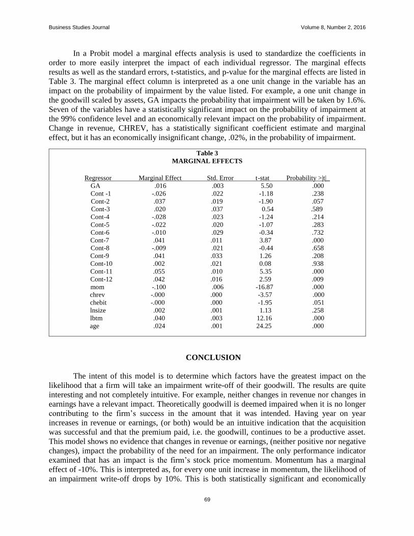
Business Studies Journal Volume 8, Number 2, 2016
69
In a Probit model a marginal effects analysis is used to standardize the coefficients in
order to more easily interpret the impact of each individual regressor. The marginal effects
results as well as the standard errors, t-statistics, and p-value for the marginal effects are listed in
Table 3. The marginal effect column is interpreted as a one unit change in the variable has an
impact on the probability of impairment by the value listed. For example, a one unit change in
the goodwill scaled by assets, GA impacts the probability that impairment will be taken by 1.6%.
Seven of the variables have a statistically significant impact on the probability of impairment at
the 99% confidence level and an economically relevant impact on the probability of impairment.
Change in revenue, CHREV, has a statistically significant coefficient estimate and marginal
effect, but it has an economically insignificant change, .02%, in the probability of impairment.
Table 3
MARGINAL EFFECTS
Regressor Marginal Effect Std. Error t-stat Probability >|t|_
GA .016 .003 5.50 .000
Cont -1 -.026 .022 -1.18 .238
Cont-2 .037 .019 -1.90 .057
Cont-3 .020 .037 0.54 .589
Cont-4 -.028 .023 -1.24 .214
Cont-5 -.022 .020 -1.07 .283
Cont-6 -.010 .029 -0.34 .732
Cont-7 .041 .011 3.87 .000
Cont-8 -.009 .021 -0.44 .658
Cont-9 .041 .033 1.26 .208
Cont-10 .002 .021 0.08 .938
Cont-11 .055 .010 5.35 .000
Cont-12 .042 .016 2.59 .009
mom -.100 .006 -16.87 .000
chrev -.000 .000 -3.57 .000
chebit -.000 .000 -1.95 .051
lnsize .002 .001 1.13 .258
lbtm .040 .003 12.16 .000
age .024 .001 24.25 .000
CONCLUSION
The intent of this model is to determine which factors have the greatest impact on the
likelihood that a firm will take an impairment write-off of their goodwill. The results are quite
interesting and not completely intuitive. For example, neither changes in revenue nor changes in
earnings have a relevant impact. Theoretically goodwill is deemed impaired when it is no longer
contributing to the firm’s success in the amount that it was intended. Having year on year
increases in revenue or earnings, (or both) would be an intuitive indication that the acquisition
was successful and that the premium paid, i.e. the goodwill, continues to be a productive asset.
This model shows no evidence that changes in revenue or earnings, (neither positive nor negative
changes), impact the probability of the need for an impairment. The only performance indicator
examined that has an impact is the firm’s stock price momentum. Momentum has a marginal
effect of -10%. This is interpreted as, for every one unit increase in momentum, the likelihood of
an impairment write-off drops by 10%. This is both statistically significant and economically

Business Studies Journal Volume 8, Number 2, 2016
70
relevant. Of all the regressors analyzed, momentum is the factor with the biggest impact on the
likelihood of impairment.
The variables with the next largest impact on the need for impairment are the CONT11
and CONT12 variables. These represent a period of 11 months and 12 months of contraction for
the prior twelve month period. They impact the likelihood of impairment by 5.5% and 4.2%
respectively. Again these are both statistically significant and economically relevant results. This
implies that some of the key components of the need for an impairment write-off are outside the
control of the firm. A contraction of 7 months is also relevant and significant, with a 4.1%
impact. Since this variable was categorized into 12 unique variables it can be seen that the
contraction period length is not statistically significant until the longer periods. This is an
intuitive result as the goodwill impairment assessment requires that the fair value of the reporting
unit be used in the assessment along with the book value of the goodwill. Thus, the assessment
includes a relative measure for the reporting unit value and an absolute measure for the goodwill
value. Consequently, a lengthy contraction period would be expected to negatively impact the
fair value of the reporting unit, yet it would have no impact on the absolute value of the
goodwill, making impairment more likely.
Of the firm characteristic variables the most impactful is the book-to-market equity value,
lBTM. A one unit increase in lBTM drives a 4% increase in the probability of impairment. This
suggests that value firms, (firms with high book-to-market equity) are more likely to take
impairment than growth firms. Yet the size of the firm has no statistically significant impact on
the probability of impairment.
For the firm characteristics related to the goodwill itself, the age of the goodwill is more
impactful to the likelihood of it being written down than the amount. The age of the goodwill,
AGE, has a 2.4% impact on the probability while the amount of goodwill, GA, has only a 1.6%
impact.
This model suggests that firms with the highest potential of an impending goodwill
impairment write-off are value firms that have negative momentum in their stock price and have
goodwill that has been on the balance sheet for the largest number of years. The model also
suggests that the likelihood of impairment increases as the length of the economic contraction
increases. Thus investors may want to consider short strategies for value firms with aged
goodwill when making investment choices in a contracting economic state.
REFERENCES
Bartov, E., F. W. Lindahl and W. E. Ricks. (1998). Stock Price Behavior Around Announcements of Write-Offs.
Review of Accounting Studies 3, 327-346.
Bens, Daniel A., and Wendy Heltzer, (2005). The Information Content and Timeliness of Fair Value Accounting:
An Examination of Goodwill Write-offs Before, During and After Implementation of SFAS 142. Working
Paper, University of Chicago.
Cheng, Ying Mei, David Peterson, and Karen Sherrill. (2012). Admitting Mistakes Pays: The Long Term Impact of
Goodwill Impairment Write-offs on Stock Prices. Journal of Economics and Finance. 2015.
Fama, Eugene F., and Kenneth French, (2008). Dissecting Anomalies. Journal of Finance 63, 1653–1678.
Hirschey, M., and V. Richardson. (2003). Investor Underreaction to Goodwill Write-Offs. Financial Analysts
Journal, 2003, 75-84.
Li K. and G. Meeks. (2006). The impairment of purchased goodwill: effects on market value. Working Paper,
University of Cambridge.

Business Studies Journal Volume 8, Number 2, 2016
71
Lys, Thomas, Linda Vincent, and Nir Yehuda. (2011). The Nature and Implications of Acquisition Goodwill.
Working paper, Northwestern University.
National Bureau of Economic Research. (2012). U.S. Business Cycle Expansions and Contractions.
http://www.nber.org/cycles.html.
Shalev, Ron. (2009). The Information Content of Business Combination Disclosure Level. Accounting Review,
84(1), 239-270.

Business Studies Journal Volume 8, Number 2, 2016
72
FOUR PROOFS IN OPTION PRICING
Garland Simmons, Stephen F. Austin State University
ABSTRACT
Many very good finance students will get to graduate school unprepared to read a logical
proof, and yet logical proof is the essential tool that is required to produce finance theory. This
paper is designed to help these students to learn how to read and understand logical proofs. To
this end, four original proofs in option pricing theory are presented. Much attention is given to
the logic of the material conditional: what it means to say, if A is true then B must be true. Four
different proof techniques are studied: direct proof, contrapositive proof, proof by contradiction
(reductio ad absurdum), and proof by cases. An appendix is also provided that sketches out the
historical development of attitudes toward theorem and proof work.
Were one to only count the number of finance journal articles published, one would
conclude that finance is in large part an empirical discipline. Nevertheless, the large, important
ideas in finance do not come from empirical studies. They come instead from theorem and proof
work. Moreover, it also true that empirical work is not often successful in speaking to the quality
of finance theory. Consider the famous case of the Sharpe (1964), Lintner (1965) Capital Asset
Pricing Model, the CAPM, a theory produced by methods of theorem and proof that has been the
subject of many, many empirical tests, yet none of these tests have been decisive.
Empirical testing of financial pricing models is often justified because some of the
economic assumptions on which the logical derivations of asset pricing models depend are
unrealistic: economic assumptions nominated only in the hopes that empirical, testable results
could be obtained, not for any other reason. Freidman (1953) champions such a positive
approach to model building, maintaining that what matters is the empirical tests of model
predictions, not the realism of the economic assumptions. But decisive empirical testing of
financial models is difficult to come by. As a case in point, the empirical testing of CAPM
results that had been counted upon to sit as judge and jury concerning the validity of theory is
itself called into serious question.
So perhaps Friedman (1953) is wrong. Perhaps the understanding that we seek as to why
security prices in financial markets behave as they do can only come from logically derived
models, like the CAPM and like the Black Scholes (1973) Option Pricing Model. If so, what is
needed by those who study finance is not better econometrics but a closer attention to the logical
derivation of theoretical results. To this end, this paper is about logical foundations of proof.
The study of the propositions and the proofs that follow are motivated by the earlier work of
Merton (1973) and of Jarrow & Turnbull (2000).
ARBITRAGE AND OPTION PRICING
Underlying assets (stocks, bonds, commodities, and so forth) trade in financial markets.
The price of each underlying fluctuates as supply and demand conditions dictate. Investors who
purchase these underlying are said to take a long position in the underlying. In this paper the
symbol S(t) designates the market value of a long position in an underlying as of time period t.
If an investor purchases one share of General Electric common stock (GE) today for $30 per
Business Studies Journal Volume 8, Number 2, 2016
73
share, one could use the notation of this paper and write an equation: S(t) = $30 in order to
describe this transaction. This notation is capable of being more specific in regard to time. If the
time period of this purchase were today, then in a timeline one might describe the time of
purchase as t = 0. In the notation of this paper one puts these ideas of time and dollar size
together and writes: S(0) = $30. The future is unknown by investors, but perhaps it will be true
that one period from now (T = 1) that the investor who today (t = 0) had purchased one share of
GE for $30 sees one period from now that the market price of GE has increased to $40 per share.
One could write this future value of a long position in GE as S(T) = $40. In the logical proofs of
this paper, the results are not specific to any specific underlying or any specific future time
period, so the symbol S(0) refers to the market value of a long position in some quantity of some
underlying today where t = 0, and the symbol S(T) refers to the market value of a long position
in that same underlying as of some point on a timeline T periods from now.
Contracts for the delivery of underlying also trade in financial markets. These too have
market prices and these contract prices also fluctuate as market conditions change. The future
value of these contracts are each a function of the future value of their corresponding underlying
asset. There are different kinds of contracts for delivery that reference an underlying: futures
contracts, forward contracts, swap contracts, and option contracts. No matter the kind of contract,
terms of delivery always include a future delivery time, a delivery place, a delivery price, and
whether or not delivery is to be done at the option of the party who purchased the contract.
Futures contracts, forward contracts, and most kinds of swap contracts have no option feature.
In this paper the problem at hand is that of option pricing. In this regard, there are four
kinds of options relevant to the proofs of this paper: European call options, American call
options, European put options and American put options. Surprisingly to the uninitiated, the
modifying terms American and European do not refer to geography in any way. These modifying
terms instead define contractual provisions in option contracts. More about this is found below.
A European call option gives any purchaser of the contract, a right, but not an obligation,
to call for delivery of the underlying on the expiry date = T and pay K dollars to the seller of the
European call option at expiry for this underlying. Should the purchaser of a call option choose
to compel delivery then that purchaser is said to exercise the option. This future date T, the
expiry day of the contract, and the delivery price K, commonly called the exercise price, are both
known by both buyer and seller of the call option at time t = 0, the day this call option is sold by
the seller of the call to the buyer of the call.
A purchaser of a European call option is said to have the long position. The long position
on the expiry day of the European call option must make a decision whether or not to exercise
the option to command delivery of the underlying. Exercise is not required: the long position is
not required to command delivery of the underlying and pay to the seller the exercise price K.
But, if the long position does not exercise, then the call option expires worthless. Even so, the
seller of the call option, the short position, keeps the money that was paid by the long position
for the call option.
The price paid by the long position for the European call option is written c(0). The
future value at expiry for the long position is c(T). The future value at expiry of the long position
in a European call option is: c(T) = Max [ S(T) - K, 0 ]. The price received by the short position
for the sale of the European call option is symbolized with a negative - c(0) and the
corresponding future value is written with a negative: - c(T) = - Max [ S(T) - K, 0 ].
Consider a specific example to see how a European call option works. Suppose that the
long position buys a call option today t = 0 on an underlying, one share of GE common stock.
Business Studies Journal Volume 8, Number 2, 2016
74
Currently, at the time of purchase, the underlying, GE common stock is worth $30 per share.
Therefore, given this as an assumption for this example, S(0) = $30. In this example assume as a
given that the exercise price K which is agreed to under the terms of the contract is equal to $34
per share and also assume as given that the expiry date of the contract is one period from today.
So by these assumptions T =1 and K = $34.
The future price of GE common stock at T = 1 is unknown at present, so S(T) = ? But, if
at expiry, one period from now, GE is worth more than K, then the long position should choose
to exercise their option which then would compel the seller of the call option to deliver the
underlying and accept in payment the exercise price K = $34, thereby producing a payoff at
expiry equal to $6 = $40 - $34 = S(T) - K. On the other hand, if a year from now at expiry the
underlying GE trades at a price equal to or less than K, say S(T) = $32 instead of S(T) = $40,
then the long position should permit the option contract to expire worthless and no payoff at
expiry will be generated. The seller of the call option, the short position, keeps the price paid for
the European call option, c(0), no matter what, even when the option contract expires worthless.
The delivery terms of American call option contracts differ from European call option
contracts in only one respect: the long position in the American call may choose to exercise at
any time after the American call is purchased up until the expiry day is over (0 < t ≤ T). The
price paid by the long position for the American call option is symbolized C(0). The future value
of the long position in a American call option is designated: C(t) = Max [ S (t) - K, 0 ]. The price
received by the short position for the sale of the American call option is symbolized - C(0) and
the corresponding future value: - C(t) = - Max [ S(t) - K, 0 ].
Put option contracts are different from call option contracts. A European put option for
the delivery of an underlying gives the purchaser of the put (the long position), a right, but not an
obligation, to sell the underlying asset at expiry in for K dollars. Should the long position of a
European put choose to compel the sale of the underlying then that option is said to be exercised.
This future date T, the expiry day of the contract, and the delivery price K, commonly called the
exercise price, are both known by both buyer and seller of the put option contract at time t = 0,
the day a put option is sold.
On the expiry day of the European put option contract, the long position must make a
decision whether or not to exercise the option. Exercise is not required: the long position is not
required to make delivery of the underlying and receive from the seller of the put option the
exercise price K. But, if the long position does not exercise the option at expiry, day T, then the
contract expires and becomes worthless. Even so, the seller of the put option, the short position
keeps the money that was paid by the long position for the put.
The price paid by the long position for the European put option contract is written p (0).
The future value at expiry for the long position is p(T). The future value at expiry of the long
position in a European put option is: p(T) = Max [ K - S(T), 0 ]. The price received by the short
position for the sale of a European put option is symbolized with a negative sign – p(0). The
corresponding future value is also written as a negative number: - p(T) = - Max [ K - S(T), 0 ].
Consider a specific example to see how a European put option works. Suppose that the
long position buys a put option today t = 0 on an underlying, one share of GE common stock.
The price of this European put option is equal to p(0) at t = 0. Currently, at the time of purchase
of this put, the underlying, GE common stock is worth $30 per share. Therefore, for this
example, S(0) = $30. In this example assume as a given that the exercise price K is equal to $34
per share and also assume as given that the expiry date of the contract is one period from today.
So T =1 and K = $34.

Business Studies Journal Volume 8, Number 2, 2016
75
The future price of GE common stock at T = 1 is unknown at present. But, if at expiry,
one period from now, GE is worth less than K, say for the sake of this example S(T) = $25 then
the long position will choose to exercise their option which compels the seller of the option to
purchase the underlying for the exercise price K. Should this state of the world obtain, the long
position produces a payoff at expiry: $9 = $34 - $25 = K - S(T). On the other hand, if one period
from now at expiry GE trades at a price equal to or greater than K, then the long position will
permit the put to expire worthless. The short position keeps the price paid for the European put
option, p(0) no matter what, even if this put expires worthless.
The delivery terms of American put option contracts differ from European put option
contracts in only one respect: the long position in the American put may choose to exercise at
any time after the put is purchased until the expiry day is past (0 < t ≤ T). The price paid by the
long position for the American put option is symbolized P(0). The future value of the long
position in a American put option is designated: P(t) = Max [ K - S(t), 0 ]. The price received by
the short position for the sale of the American put option is written as a negative: - P(0) and the
corresponding future value is also negative: - P(t) = - Max [K - S(t), 0].
The proofs of this paper, in addition to the notions of call and put options discussed
above, make use of four additional concepts from finance: portfolios, synthetic positions, the
Law of One Price, and arbitrage. A portfolio is a collection of assets owned by an investor.
Some portfolios contain only a single asset, but portfolios can and often do contain many assets.
Some assets are held by investors as long positions: for example, underlying assets purchased in
the hope that they will produce income and/ or capital gains, purchased call options, and
purchased put options. Ceteris paribus, the long position in the call option desires the underlying
to increase in value, while the owner of the put option desires the underlying decline. Other
assets may be held within a portfolio as short positions. For example, an investor known as a
short-seller borrows an underlying asset, sells it, and then later repurchases it in hopes that the
underlying asset declines in value. Other short positions include selling a call option or selling a
put option. The short position in the call option benefits from a decline in the value of the
underlying, but the short position in the put option benefits from an increase in the value of the
underlying. To understand the content of an investor’s portfolio, one must know the market value
of each asset contained by the portfolio and which assets are held as long positions and which are
held as short positions.
Portfolios can also contain synthetic positions. A synthetic position is a portfolio of long
and short positions that produces future values that are equal to the future value of another asset
in every possible future state of the world. Consider an investor who wishes to create a synthetic
position that will produce a future value on some expiry date equal to the future value of an
underlying asset on that same date. If this underlying produces no income prior to expiry, then
this investor can solve this problem of replicating the future value of an underlying by taking
positions in three assets: purchase a European call on the underlying, sell a European put on the
same underlying with the same exercise price and the same expiry as the call, and purchase a risk
free asset with future value equal to the exercise price of the call and the put at expiry. This
portfolio thus created by the investor is a synthetic position. It produces the same future value of
the underlying at expiry in every possible state of the world.
The Law of One Price holds that assets and portfolios which have identical future values
in every possible state of the world must also have identical price. Take two assets, say General
Electric common stock and Wal-Mart common stock, if these two assets were to produce the
same future values in every possible state of the world, then, by the Law of One Price, they both

Business Studies Journal Volume 8, Number 2, 2016
76
must sell for the same price. Since they do not produce identical future values, they sell for
different prices. Now consider the example above, the investor who creates a synthetic position
in an underlying. Since this synthetic position (a long position in a call, a short position in a put,
and a long position in a risk free asset) replicates the future values of the underlying, the Law of
One Price holds that the price of the synthetic position must equal the price of the underlying.
In markets where investors are permitted to trade at no cost, the Law of One Price should
hold. To see why, consider the opposite case. What if the Law of One Price does not hold true?
Consider two assets, both with identical future values in every possible state of the world. Yet
one of the assets has a higher price than the other. If this were true, then two things happen: first,
investors simultaneously buy the cheaper of the two and take a short position in the more
expensive, and then second, at some future point in time, close both positions -- sell the long
position and use the proceeds of this sale to cover the short position. This first action of buying
low and selling high produces a positive cash flow to the investor. This second action of selling
the long position and covering the short produces a zero cash flow. This investment strategy is
ended with the investor making a risk free profit in the first step and getting out of the market in
the second step at no cost. With no investment the investor has generated a risk free profit, and
has done so with no risk. No matter which way the market moves before the investor exits in step
two, the future values of the long and short positions offset each other, so the net result is zero
gain or loss. That is why there is no risk. So if the Law of One Price fails, investors make money
with no net investment and no risk. If markets are working properly, in equilibrium, the Law of
One Price holds true. In properly functioning markets, investors will compete with one another to
buy the cheaper asset, thereby driving its price up; and sell the higher priced, thereby driving its
price down. This continues until equilibrium is reached: assets with identical future values in
every possible state trade at the same price.
Consider an investor who creates a synthetic position that mimics an underlying. (The
underlying of this example produces no income prior to expiry.) This synthetic position is
constructed so that it produces a future value at expiry exactly equal to the future value of an
underlying. The synthetic position is itself a portfolio containing three assets: a long position in a
European call option for the delivery of an underlying, a short position in a European put option
for delivery of the same underlying and with equal an exercise price equal to that of the call, and
a risk free investment large enough to produce a future value equal to this common exercise
price. The left-hand side of the equation below describes this future value of the synthetic
position at expiry and the right-hand side describes the future value of expiry of the underlying.
The first term of the left-hand side is the future value of the long-position in the European call,
the second, the future value of the short-position in the European put, and the third term is the
future value of the risk free investment:
Max [ S(T) – K, 0 ] – Max [ K – S(T), 0 ] + K = S(T)
No matter the value of S(T) or K the synthetic position produces a future value equal to
the future value of the underlying. To see this let the exercise price K = $34 and let S(T) vary
from $1 to $100. In every case the left-hand side of the equation above equals the right-hand
side: in every case, at expiry, the future value of the synthetic position equals the future value of
the underlying.
Now consider the consequences of the illustration of the previous paragraph for
equilibrium in capital markets. There are only two possible cases to be considered. Case one: if
Business Studies Journal Volume 8, Number 2, 2016
77
the price of the synthetic position is equal to the price of the underlying, then there is no
incentive to prefer one over another because all of the possible the future values at expiry for the
synthetic position are equal to those of the underlying. So the risk and the possible returns for
both investments are exactly the same. Case two: if the price of the synthetic position is not equal
to the price of the underlying, then investors should prefer a long position in the cheaper
alternative and also prefer a short position in the more expensive choice. In equilibrium prices
adjust such that the price of the synthetic position equals the price of the underlying.
The ability of investors to create synthetic positions using call and put options and risk
free investments is closely related to the concept of arbitrage. Arbitrage has three essential
properties. If an investor can construct a portfolio that costs nothing, has no risk, and yet
produces a profit, then this investor has successfully executed an arbitrage strategy, and the
profits of this strategy are known as arbitrage profits. Synthetic positions are created by investors
in order to generate arbitrage profits. If the price of the synthetic position is not equal to the price
of the underlying, then arbitrage profits are available. On the other hand, if the price of the
synthetic position is equal to the price of the underlying, then no arbitrage profits are available.
Although investors have a personal interest in arbitrage, academicians look at the
consequences of the ability of investors to generate arbitrage profits in order to explain how and
why prices for call and put options behave as they do. Black and Scholes (1973) in work later
recognized with a Nobel Prize in economics devised a logical argument connecting synthetic
positions and arbitrage to option pricing. They show that calls and puts are priced such that no
opportunities for arbitrage profits exist. Their argument remains influential in the later proofs of
other scholars who work in option pricing. The proofs of this paper continue in that tradition.
SOME LOGICAL BACKGROUND
Theorem and proof work answers the question why one should believe that something is
true, even in the absence of empirical data analysis. A logical proof is always concerned with
how the truth of one statement affects the truth of another statement. A proof argument is a
collection of statements where the proposition to be proven is the conclusion. The statements that
justify the conclusion are called premises. Given the truth of the premises, a proof is a guarantee
of the truth of the conclusion. Clear thinking in a logical proof first lays bare the justification for
a conclusion, the premise statements that describe what is known or what is assumed to be true
about reality. If each of the premise statements leading up to the conclusion is true, then the
conclusion must also be true. On the other hand, if one or more than one of these premise
statements are false, then the conclusion may be true or it may be false.
Some statements that can be used in proof arguments are necessarily true, true in every
possible state of the world. Aristotle distinguishes between de dicto necessity and de re
necessity. Statements that are necessarily true de re are true by virtue of definition. Consider the
balance sheet equation as a first example, total assets equal total debt plus total equity. Consider
now de re necessity. As a second example, the statement – the market portfolio contains all risky
assets – is true as a matter of de re necessity. Why is this so? One of the essential properties of
the market portfolio is that it contains all risky assets, essential in the sense that if this property is
removed from this concept, the market portfolio, then its meaning is destroyed. (Whatever might
remain after this portfolio is reduced can be something else, but it is no longer possible for this
something else to be the market portfolio). Statements which are true as a matter of de re
necessity are immune to any empirical efforts which might be mounted to disprove them. So, one
can say that whether or not the value of the market portfolio can be measured with empirical
Business Studies Journal Volume 8, Number 2, 2016
78
means, there is, both as a matter of concept and as a matter of fact, such a thing called the market
portfolio. The same kinds of things can be said of the efficient set, systematic and unsystematic
risk. These proof-generated concepts found in CAPM theory all are defined by their essential
properties which obtain in every possible state of the world, including those of the real world. In
this way it can be said that these theoretical objects exist both in theory and in reality as a matter
of de re necessity.
By contrast, the matter of de dicto necessity is concerned with logical entailment, the
relationship of the conclusion of an argument to the premises of that argument. As a second
example of de dicto necessity, consider a logical consequence of the CAPM made famous by
Roll (1977): given that the CAPM is true, the market portfolio is mean-variance efficient. This
statement is true de dicto, for if the assumptions under which the CAPM is logically derived are
all true, then it must be the case that the market portfolio is mean-variance efficient. The only
legitimate way to deny the mean-variance efficiency of the market portfolio is to also deny the
truth of one or more of the assumptions underlying the CAPM. Denial of the dictum, the
conclusion, always entails denial of one (or more than one) of the premise statements used in
order to justify the conclusion.
These two notions de re and de dicto necessity do not exhaust the concept of necessity.
There are statements which are necessarily true that are not true as a matter of definition and not
true in the same way that a conclusion which follows of necessity from its premises is true.
Consider the following statement as an example – at present, human beings command limited
economic resources. One would be hard put to posit a state of the world where this statement is
false. If one claims that this statement is true in every possible state of the world, then one claims
that this statement is necessarily true.
Some arguments produce conclusions that rest on assumptions contained within the
premises that make sense in the real world, but some do not. Unrealistic assumptions put the
conclusion in question. Belief is a matter of choice. This choice to believe or to refuse to believe
is described in modern philosophy in connection with the notion of a warranted belief. Plantinga
(1993) describes three essential properties of what is meant by this concept, a warranted belief.
First, for a belief that a statement is true to be warranted this statement must be true. Second, the
person considering this statement must believe that it is true. And third, this person must be
justified in believing it to be true. This first requirement is a matter of truth or falsehood, the
second a matter of opinion, the third a matter of evidence. The strength of an individual’s
opinion concerning the truthfulness of some statement varies with the quantity and quality of
evidence available and their interpretation of that evidence.
PROOFS IN OPTION PRICING
Consider the proof below, a direct proof which moves from an assumption, step-by-step,
to a conclusion. The first statement, labeled Result I, is the proposition to be proven true by the
proof argument which follows it. Thus it is claimed that the proposition is true de dicto, which
means that it must be true in the same states of the world where all of the premises contained in
the proof argument justifying this conclusion are first true.
This Result I is a specific kind of statement, a material conditional. Material conditional
statements are of the form if A is true, then B must be true. The A part is called the hypothesis of
the material conditional, and the B part is called the consequent of the material conditional. The
hypothesis of Result I below is a conjunction that has two parts, first that the price of an
underlying is equal to zero and second that no arbitrage profits are possible. And the consequent

Business Studies Journal Volume 8, Number 2, 2016
79
of the proposition below is also a conjunction of two parts, first that the price of an American
call option written on that underlying asset is equal to zero and second that the future value of the
underlying is equal also equal to zero.
Result I
If S(0) = 0 and if there are no arbitrage profits, then C(0) = 0 and S(0 < t ≤ T) = 0.
Proof
By hypothesis we are only considering circumstances where two things are both true:
S(0) = 0 and there are no arbitrage profits. The truth of these two sentences require that C(0) = 0.
Why? Investors in their desire to create arbitrage profits, create a two asset portfolio purchasing
S(0) and selling C(0). Recall, by hypothesis we are considering only cases where S(0) is equal to
zero. Should it also be true that C(0) is equal to zero, then there are no arbitrage profits. At t = 0
this two asset portfolio neither produces cash inflows nor requires cash outlays. By construction
in every future time period until expiry the potential payoff of this two asset portfolio is equal to
S(t) – Max [ S(t) – K, 0 ]. By definition, when no arbitrage profits are available to a portfolio
which initially costs nothing, the potential payoffs in every possible state of the world of that
same portfolio must also equal zero. This is only the case when S(0 < t ≤ 0) = 0 and C(0) = 0.
QED
Does it matter that we do not know the exact nature of underlying and the American call
option that are bought and sold by an investor? No it does not. The proof argument is very
general; it applies to anyone. Does it matter that we do not know who this investor is? Again, the
proof argument is very general, it applies to anyone. Does it matter that investors can buy and
sell without hindrance? Yes. The proof argument is driven by the assumption that there is no
hindrance to buying and selling that would stop investors from taking advantage of arbitrage
opportunities. If this is not so then the proof argument falls apart.
Below one finds an explanation of a second proof, another proposition of option pricing
theory. In this next proof the student is invited to see the connections between a finance concept,
arbitrage, and two additional logical concepts: logical equivalence and the contrapositive
statement of a material conditional. Before going on to the next proof, the concept of arbitrage is
reconsidered.
Arbitrage occurs if the Law of One Price is violated. Consider this Law of One Price
which says that if two investments produce identical future cash flows in every possible state-of-
the-world, then these two investments must have the same prices. If this law is violated, then
investors will by the cheap asset and short the expensive asset thereby creating arbitrage profits.
Arbitrage profits a risk free and without any net investment cost. It is easy to see that if arbitrage
profits could frequently be generated then traders could become immensely wealthy without
taking any risk and without investing any money. One of the major themes of modern finance
theory is that prices in capital markets will move so that arbitrage profits become non-existent.
After all when traders buy the cheap asset of the arbitrage and short the expensive asset they are
driving up the price of the cheap asset and down the price of the expensive one, so arbitrage
opportunities should be fleeting.
In the proof below the main idea is that the prices of call options and the underlying
assets on which these call options are written must move in such a way as to eliminate any
opportunities for arbitrage. In this proof there exists a call option written on an underlying asset.

Business Studies Journal Volume 8, Number 2, 2016
80
The purchaser of this call option, prior to contract expiration, has the right to purchase the
underlying asset referred to in the contract for a price equal to K. The price of this American call
option today is equal to C(0), the contractual exercise price is equal to K, and the price of the
underlying asset today is equal to S(0). Prior to the expiration of the option contract, the writer of
the call option will pay the purchaser on demand an amount equal to max [0, S(0) - K] which is
the maximum of two numbers, zero or the current value of the underlying asset less the exercise
price.
As with the proof above, this proposition below is a material conditional. As you
remember, material conditional statements are of the form: if A is true, then B must be true. The
A part is called the hypothesis of the material conditional, and the B part is called the consequent
of the material conditional. The hypothesis of the proposition below is: there are no arbitrage
opportunities. The consequent is: C(0) ≥ Max [ S(0) – K, 0 ]. This proposition is rewritten as the
contrapositive statement of this material conditional statement.
Result II
If there are no arbitrage opportunities, then C(0) ≥ Max [ S(0) – K, 0 ].
Proof
Rewrite the proposition above in the contrapositive: If C(0) < Max [ S(0) – K, 0 ] then
there are arbitrage opportunities. By hypothesis of the contrapositive statement one may say that
we are only considering cases where it is true that: C (0) < Max [ S(0) – K,0 ]. See if arbitrage
exists in these circumstances by trying to create arbitrage profits:
(1) Immediately borrow an amount of money = C(0).
(2) Immediately buy C(0) with the borrowed money. Net investment is equal to zero.
(3) Exercise immediately and receive S(0) - K.
(4) Sell S(0) - K.
(5) Immediately repay loan. Investment positions are closed – thus there is no risk.
Profit is equal to S(0) - K - C(0) which is positive when C(0) < S(0) - K. An arbitrage
profit has been created in these circumstances. Why? Net investment of zero produces a risk free
profit. This is what is meant by arbitrage. The contrapositive has been shown to be a true
statement. By logical equivalence it must also be that the original proposition is also a true
statement.
QED
The contrapositive of the material conditional has the form: If the negation of B is true,
then the negation of A must be true. B is written: C(0) ≥ Max [ S(0) – K, 0 ]. The negation of B
is what must be true when B itself is false. So the negation of B is written: C(0) < Max [ S(0) –
K, 0 ]. Now consider A: there are no arbitrage opportunities. The negation of A is what must be
true when A itself is false. So, the negation of A: there are arbitrage opportunities. Putting all this
together for the proof work below, one may write the contrapositive of the proposition statement
like this: If C(0) < Max [ S(0) – K, 0 ] then there are arbitrage opportunities.
When two statements are logically equivalent to one another they each have identical
meanings, even though they may appear to not mean the same thing at all. The material
conditional statement, IF A is true, then B must be true, is logically equivalent to its

Business Studies Journal Volume 8, Number 2, 2016
81
corresponding contrapositive statement, If not B is true, then not A must be true. This means that
the two statements (IF A is true, then B must be true) and (If not B is true, then not A must be
true) have identical meanings in every possible circumstance. Why is this important? If one
proves that the contrapositive is true, then one has also proven that the other is true too. The
application here to this proof above is straightforward. In the proof above, the proposition: If
there are no arbitrage opportunities, then C(0) ≥ Max [ S(0) – K, 0 ] is logically equivalent to If
C(0) < Max [ S(0) – K, 0 ] then there are arbitrage opportunities. Since the contrapositive is
proven true then so is the original proposition proven to be true.
A proof by contradiction (reductio ad absurdum) works on the negation of a proposition
that one wishes to prove to be true. If one can prove that the negation is false then it must also be
that the original proposition is true. In this way, Result III below works on the negation of a
material conditional (if A is true, then B is true). The negation of a material conditional can be
written is several ways. The proof below writes the negation of if A is true then B is true as a
conjunction: A is true and B is false. Specifically, consider the negation of the proposition: there
are no arbitrage opportunities and c(0) S(0) + p(0) - B(0,T) K. This proposition and its
negation cannot both be true, and yet one must be true. If the negation is true then the original
proposition above must be false. On the other hand, if the negation is false, then the original
proposition above must be true. The task at hand is to show that this original proposition is true.
This will be accomplished in the proof below by showing that the negation of this original
proposition is false. This approach to proof is known as proof by contradiction.
Result III
If there are no arbitrage opportunities then c(0) = S(0) + p(0) - B(0,T) K.
Proof
The negation: there are no arbitrage opportunities and c(0) S(0) + p(0) - B(0,T) K. This
is proven to be false if one could show that either there are arbitrage opportunities and either c(0)
> S (0) + p(0) - B(0,T) K or that there are arbitrage opportunities and c(0) < S(0) + p(0) - B(0,T)
K. If c(0) > S (0) + p(0) - B(0,T) K, then one can create an arbitrage portfolio, one which
produces a positive cash inflow initially at t = 0 and a zero cash outflow at expiry, t = T. That is
to say this portfolio requires no net investment and yet produces an immediate risk free cash
inflow and no cash outflows, ever. It is now our task to prove that we can create this arbitrage.
To do this we have to demonstrate how a portfolio can be created which will require no net
investment and produce a net cash inflow with no risk. We create this arbitrage by doing the
following. Initially, at t = 0, sell c(0) and buy [ S(0) + p(0) - B(0,T) K ]. This gives us a positive
cash inflow when c(0) > S(0) + p(0) - B(0,T) K. So when we sell the call and buy the synthetic
position there is then no net investment required and a risk free positive cash flow is generated.
At expiry, t = T, one of only two things can happen. It will either be true that S(T) > K or that
S(T) ≤ K. First, let’s evaluate the future values of our portfolio that is created at time period zero
under the assumption that S(T) > K.
Case I
If S (T) > K, then the portfolio that we created will produce the following future values at
expiry, t = T. The equation of future values written below is ordered in the following manner: the

Business Studies Journal Volume 8, Number 2, 2016
82
future value of the short position in the call, the future value of the long position in the
underlying, the future value of the long position in the put, and the last term on the left-hand side
of the equation below is the future value of the short position in a risk free asset.
[ - S (T) + K ] + S (T) + 0 - K = 0.
So, If S(T) > K, then the portfolio that we created will produce on net a zero future value.
And at expiry, t = T, we, the owners of this portfolio, will no longer be obligated in anyway, we
will no longer have any investment positions open. As a result the profits generated at t = 0 are
kept safe.
Case II
If S(T) ≤ K, then the same portfolio that we created initially at t = 0 will produce the
following (different) future values at expiry, t = T. Again, the equation of future values written
below is ordered in the following manner: the future value of the short position in the call, the
future value of the long position in the underlying, the future value of the long position in the
put, and the last term on the left-hand side of the equation below is the future value of the short
position in a risk free asset.
0 + S(T) + [ K - S(T) ] - K = 0.
So, If S(T) ≤ K, the future value of the portfolio is equal to zero in Case II. As a result the
profits generated at t = 0 are kept safe. Either Case I or II must obtain. In both cases arbitrage
profits are kept safe. Therefore, the negation statement: there are no arbitrage opportunities and
c(0) S(0) + p(0) - B(0,T) K is shown to be false. Clearly, there are arbitrage opportunities when
c(0) S(0) + p(0) - B(0,T) K. Since the negation is shown to be false, the original proposition is
proven true.
QED
Result IV below is a direct proof that uses the proof by cases technique. The cases that
are employed to drive a proof are mutually exclusive of one another, and any listing of these
cases is exhaustive. Too see how this approach might work, consider the sentence x is not equal
to y. Such consideration would likely focus on two separate cases. In the first case x is less than
y and in the second case x is greater than y. There is no third case because the first two are
mutually exclusive of one another and, taken together, exhaustive.
Result IV
If there are no arbitrage opportunities then c(0) = S(0) + p(0) - B(0,T) K
Proof
The concept of “no arbitrage” admits to an essential property: portfolios that have zero
present values produce zero future values in every future state of the world. The portfolio that we
choose to consider is a short position in a European call, a long position in the underlying, a long
position in a European put, and a short position in a risk free asset:

Business Studies Journal Volume 8, Number 2, 2016
83
-c(0) + S(0) + p(0) - B(0,T) K
This portfolio produces a zero future value in every future state. To see this consider
Cases I and II below.
Case I
Consider future states of the world where S(T) > K.
If S(T) > K, then the portfolio that we created will produce the following future values at
expiry, t = T. The equation of future values written below is ordered in the following manner:
the future value of the short position in the call, the future value of the long position in the
underlying, the future value of the long position in the put, and the last term on the left-hand side
of the equation below is the future value of the short position in a risk free asset.
[ - S(T) + K ] + S(T) + 0 - K = 0.
So, If S(T) > K, the future value of the portfolio is equal to zero in Case I.
Case II
Consider future states of the world where S(T) ≤ K.
If S(T) ≤ K, then the same portfolio that we created initially at t = 0 will produce the
following (different) future values at expiry, t = T. Again, the equation of future values written
below is ordered in the following manner: the future value of the short position in the call, the
future value of the long position in the underlying, the future value of the long position in the
put, and the last term on the left-hand side of the equation below is the future value of the short
position in a risk free asset.
0 + S(T) + [ K - S(T) ] - K = 0.
So, If S(T) ≤ K, the future value of the portfolio is equal to zero in Case II. Either Case I
or II must obtain. In both cases the future values are equal to zero. Given that there are no
arbitrage opportunities it is also the case that the present value of the portfolio under
consideration is equal to zero.
-c(0) + S(0) + p(0) - B(0,T) K = 0
If there are no arbitrage opportunities then c(0) = S(0) + p(0) - B(0,T) K.
QED.
CONCLUSION
Theorem and proof work answers the question why one should believe that something is
true. A logical proof is an argument that justifies belief in a proposition. There are different kinds
of logical proof. A direct proof moves from an assumption step-by-step to a conclusion that must
be true if the initial premises are first true. A proof by contradiction (reductio ad absurdum)
works on the negation of a proposition that one wishes to prove to be true. If one can prove that

Business Studies Journal Volume 8, Number 2, 2016
84
the negation is false then it must also be that the original proposition is true. A proof of a
material conditional by the proof of its contrapositive equivalent is used when direct proof is
difficult. A proof by cases approach divides a difficult proposition into separate, mutually
exclusive parts so that the proof of this difficult proposition can also be divided.
REFERENCES
Black, F. and M. Scholes (1973). The Pricing of Options and Corporate Liabilities. Journal of Political Economy,
81(3), 637-654.
Fama, E. F., and K. R. French (1996). The CAPM is Wanted, Dead or Alive. Journal of Finance, 51(5), 1947-1958.
Fama, E. F., and K. R. French (1992). The Cross-Section of Expected Stock Returns. Journal of Finance, 47(2),
427-465.
Friedman, M. (1953). Essays in Positive Economics. Chicago, Illinois: The University of Chicago Press.
Heath, Sir Thomas (1956). The Thirteen Books of EUCLID’S ELEMENTS Translated From the Text of Heiberg
With Introduction and Commentary ( 2nd
Edition). NewYork: Dover Press.
Hume, D. (1777). Enquiry Concerning Human Understanding (Third edition). Selby-Bigge, L.A. & P.H. Nidditch
eds.: London: Oxford University Press, 1975.
Jarrow, R. and S. Turnbull (2000). Derivative Securities Second Edition. Cincinnati, Ohio: South-Western College
Publishing, a division of Thompson Learning.
Levy, M., and R. Roll (2010). The Market Portfolio May Be Mean/Variance Efficient After All. Review of
Financial Studies, 23(6), 2464-2491.
Lintner, J. (1965). The Valuation of Risk Assets and the Selection of Risky Investments in Stock Portfolios and
Capital Budgets. Review of Economics and Statistics, 47(4), 13-37.
Merton, R. C. (1973). Theory of Rational Option Pricing. Bell Journal of Economics and Management Science,
4(1), 141-183.
Malcom, N. (1967). Wittgenstein, in Paul Edwards, ed.: Encyclopedia of Philosophy Vol. VIII. Macmillan Co.,
New York.
Plantinga, A. (1993). Warrant and Proper Function. London: Oxford University Press.
Plantinga, A. (1974). The Nature of Necessity. London: Oxford University Press.
Rubinstein, M., (1976). The Valuation of Uncertain Income Streams and the Prices of Options. Bell Journal of
Economics, Autumn 7(2), 407-425.
Roll, R. (1977). A Critique of the Asset Pricing Theory’s Tests; Part I. On Past and Potential Testability of
Theory. Journal of Financial Economics, 4(2), 129-176.
Sharpe, W. F. (1964). Capital Asset Prices: A Theory of Market Equilibrium Under Conditions of Risk. Journal of
Finance, 19(3), 425-442.
Wilkerson, T. E. (1976). Kant’s Critique of Pure Reason. London: Oxford University Press.

Business Studies Journal Volume 8, Number 2, 2016
85
APPENDIX
Ancient Greek philosophers preferred (and some insisted) that each step in an argument
be verified by way of empirical data analysis. In this connection both English words theorem and
theater are derived from the same ancient Greek word theoros. This word from the classical
Greek refers to a showing or to a demonstration. This word theoros was borrowed by Greek
geometers of Euclid’s day, who insisted that logical proofs of geometric propositions must begin
and end with a demonstration, a showing of the equivalence between logical results and physical
reality. The foundation of every acceptable logical proof for these geometers was an axiom
structure thought to be nothing more than an accurate description of physical reality, the truth of
which is beyond dispute. Authors of geometric proof of the time of Euclid named their
conclusion a theoros only if two standards were met. First, the logical steps in the reasoning
process must have been shown to be without defect; and second, the concluding statement of the
proof must have been verified by empirical measurement. Such a practice of demanding a
demonstration in the real-world of theoretical propositions was to these ancients a safeguard
against error.
Even apart from geometry, a poor connection between logic and empirical reality in
either the premises of an argument or in its conclusion rendered the reputation of that argument
tenuous. Even before Aristotle began a systematic study of logic, scholars knew that meaningless
results could be achieved with an application of a flawless logic to a foundation of flawed first
principles. Plato, among the first of the western philosophers to know that the method of an
argument can be known and studied separately from its contents, did not approve of sophists –
those who entertained in ancient Athens by creating seemingly logical arguments which
produced absurd results, which were contradicted by real-world experience. Sophists were able
to produce these entertaining arguments because they built them atop an axiom set which
contained a contradiction.
To defend logical argument from the manipulation of sophists, Plato and his
contemporaries classified arguments into two categories. Demonstration proofs were those based
in premises well-connected to physical reality. Dialectic proofs were not constrained by
empirically verifiable premises. Plato insisted that neither demonstration proofs nor dialectic
proofs contain a contradiction.
Demonstration proofs because of their strong connections to empirical reality were
thought by the great philosophers of ancient Athens to be superior to dialectical proofs.
Demonstration proofs were declared to be true always, immune from fallacy with regard to both
form and content. By contrast, dialectical arguments were considered to be provisionally true and
not immune from a contradiction which might come from a later discovery.
Euclid was very much concerned about the missing empirical connections for two of his
ten axioms used to create plane geometry. To mitigate the possible mistakes associated with
employing these two questionable axioms in theorem and proof work, Euclid was driven to
derive as many theorems as he could without relying upon either the parallel line axiom or the
axiom which states that a line segment can be extended to any length. The reluctance of Euclid to
employ these two axioms was caused by an inability to demonstrate in the real-world that they
are in fact true statements.
In fact, it was the replacement of these same two axioms which troubled Euclid and the
willingness to interpret the notion of the line of Euclid’s work as something other than a straight-
line in a plane that produced Non-Euclidian geometries, initially the separate work of three
mathematicians – Gauss, Lobatchevsky, and Bolyai. Scholars, including Gottlob Frege, Bertrand
Business Studies Journal Volume 8, Number 2, 2016
86
Russell, and Alfred North Whitehead, responded to the creation of these Non-Euclidian
geometries by doubting the ability of anyone to devise a single, unique axiom structure capable
of adequately describing reality. Thus the advent of Non-Euclidian geometry caused many
scholars to permit the divorce of mathematical space from physical space. If these two spaces are
separate concepts, then the knowing of physical space is beyond the reach of pure
mathematicians and at the same time irrelevant to their explanations of mathematical spaces. It
was left to the mathematician Kurt Gödel to cast doubt upon the mathematician’s ability to
adequately describe the workings of mathematical spaces alone.
Prior to these mathematical advances, during the Enlightenment, David Hume and James
Stuart Mill a rebelled against the notion that methods of theorem and proof could produce a
coherent theory capable of describing a physical-material world. Hume held that there could be
no such thing as logical proof. He believed that no proof argument could be understood in the
same way by different individuals and he also doubted the ability of anyone to reason by way of
a valid logical argument from an axiom structure to conclusions that could actually explain how
the real world works. So Hume opposed the work of Euclid, and he also opposed the latter works
of Galileo and of Newton, both famous during the Enlightenment for describing the workings of
the physical universe as they reasoned from an axiom structure consisting of natural laws. It was
Hume’s position that they were mistaken: there could be no such thing as causal necessity used
to explain the consistent behavior of a solar system nor could there be any such thing as logical
necessity used to explain the working of a geometric argument and the connection of that
argument to the real world.
Immanuel Kant reacted to Hume’s work. Kant’s position was that there are necessary
truths and that theorem and proof work could be useful approach in scientific research.
However, in Kant’s view, there were limits to what theorem and proof work could accomplish.
In these limits Kant sought to deny the medieval rationalism of St. Thomas Aquinas and of St.
Anselm of Canterbury, both of whom claimed to have proven with the methods of theorem and
proof alone the existence of God. It was Kant’s view that rationalism, a belief that reason alone
is capable of accurately describing what is beyond the reach of our senses, was flawed. Kant
believed that the ability of human beings to accurately describe reality with theorem and proof
was limited to matters that are understood in reference to a possible experience which someone
might have in the real world.
However, Kant did not go on to heap praise on empirical data analysis. It was his view
that empirical reality could not be understood as it really is by human experience. Instead, those
who analyze data, perceive it and organize it according to the dictates of basic preexisting
categories of the human mind. Because this process of analysis is both involuntary and
subjective, it is not within the power of anyone to see clearly empirical reality. If Kant is right
about this, then the practice of science is very difficult indeed.
Right or not, one of the vital contributions of Kant to the problem of knowing is in
terminology. Kant used two broad categories to identify statements. In describing what is
analytic, Kant followed after the work of Leibniz, who held that a valid definition of a concept
may be had by a complete listing of its essential properties. Kant agreed that theorem and proof
methods may employ analytic statements (definitions) even though these statements are immune
to experimental investigation. Knowledge of analytic statements is always a priori.
Kant classified all statements that are not analytic as synthetic. A synthetic statement is a
description of a concept in its relation to empirical reality. Kant accepted that some synthetic
Business Studies Journal Volume 8, Number 2, 2016
87
statements are knowable in the absence of experience – knowable a priori, but knowledge of
others - the synthetic a posteriori - are not understood without real world experience.
By contrast, those who are Logical positivists demand that all statements which describe
reality be justified a posteriori – be justified only after the empirical evidence is evaluated.
Logical positivism admits belief in necessary truths only in regard to language that defines or
refers to empirical objects. Beyond this limited admission, experience remains a prerequisite for
knowing the real world.
A foundational belief of logical positivism is that only a theoretical conclusion which is
connected to what can be observed in the real world could have any meaning. Therefore,
theoretical conclusions which are not referenced to physical reality should be out-of-bounds, not
worthy of scientific consideration. This is the famous verification principle of logical positivism,
attributed by Malcom (1967) to Wittgenstein, a twentieth-century philosopher who studied the
connection of language to reality.
Such a demand for verification could be a mistake. Sir Karl Popper (1959) argued that
this demand for empirical verification can never be met. Popper’s position was that verification
is an unworkable plan in any scientific program, for to verify theory with real-world data is a
matter of comparing every possible observed value to its corresponding predicted value, clearly
an impossible task when the number of possible outcomes and corresponding predictions is
large.
Popper proposed an alternative to the verification principle that would yet permit the
evaluation of theoretical predictions against real-world data. Popper’s alternative is known as
falsification, a search for empirical counterexamples in an attempt to prove a theory wrong.
Unlike the demand for verification, a search for counter-examples need not go on forever. It can
end when a sufficient number of counterexamples to theoretical predictions are found. At this
point the theory is falsified and then abandoned.
Popper’s doctrine of falsification also imposed requirements upon a theory. Popper held
that in scientific work it must be the case that theoretical predictions can be measured and
compared against actual outcomes. Much of the current discussion in philosophy of science is
concerned with how old theories are adjusted to accommodate the finding of counter-examples,
and how much evidence against a theory is to be tolerated before it is considered obsolete and
overthrown in its entirety. In any case, the existences of these empirical counter-examples are
only made possible when actual outcomes can be compared to the predictions of a theory. But
not all theories are subject to being analyzed in this way. If theoretical predictions cannot be
well-measured empirically, then they cannot be compared to actual outcomes. These theories
then have no empirical content. They cannot be verified, they cannot be falsified, and such is
arguably the case with the asset pricing models of financial economics.

Business Studies Journal Volume 8, Number 2, 2016
88
THE LECTURE/LAB COMBINATION COURSE:
AN INNOVATIVE WAY TO TEACH A LARGE
WRITING COURSE
Dr. Carol S. Wright, Stephen F. Austin State University
ABSTRACT
The lecture/lab combination class as an alternative to teaching a large section format of a
writing-intensive class, however this format has its own special challenges. This paper will
present a multiple case study of two courses and how the lecture/lab format is administered.
Findings can be used to inform administrators and instructors when offering a large section class
that involves an extensive amount of interaction between instructor and students. Examining the
unique course delivered at this university enabled the researcher to identify some significant
areas of practice beneficial for other instructors to utilize in their own course designs. Instructors
must be able to maintain a relationship with their students so that they can best deliver course
material effectively. Each class and each student is different and it is important that the instructor
is able to identify the needs and abilities of the students enrolled in their classes. The use of TAs
can be beneficial, but it is important that the instructor be involved in the class assignments to
accurately assess learning.
It is likely that universities will continue to offer large classes at various levels, but there
must be a balance between budget allocations and student learning. As the class size increases,
the chances of the class being taught as a lecture style course will increase and cause the
instructors to lose their ability to connect with students. Students are more likely to feel detached
from the subject matter if they have fewer opportunities to interact with the material being
presented.
INTRODUCTION
Change is good, or so the saying goes. Using the excuse that this is the way it has always
been done, will not hold up in an argument. Sometimes changing the way a course is delivered is
beneficial, and sometimes this change is necessitated because of budget cuts. The budget is often
a popular issue at educational institutions because administrators are worried about what the next
legislative session will decide about governmental support. Colleges have become creative in
how they have approached budget shortages by offering more online classes, cutting back staff,
eliminating programs, and teaching more students in each class.
One solution, teaching more students in a class, creates a unique environment for teachers
and students. It might not be an ideal situation, but if an educational institutional is forced to
increase class size, the lecture/lab combination class may be a suitable alternative.
Moshiri and Cardon (2014) experienced problems with class sizes at their own
institution. From 2008 to 2013, the actual class size in the business communications courses
more than doubled because the university experienced a 20% reduction in its state funding. The
possibility of other institutions facing similar budget cuts could cause other classes to increase in
size. Based on this possibility, administrators and instructors of all classes should be informed
about approaches to increased class sizes.
Business Studies Journal Volume 8, Number 2, 2016
89
Purpose Statement
The purpose of this paper is to present the lecture/lab combination class as an innovative
alternative to teaching a large section format of a writing-intensive class. Specifically, it will
look at instructor and student perceptions of how the course functions at one particular
university. Information gained from the study can be used to inform others who may be
considering a unique approach to teaching a larger class that involves an extensive amount of
interaction between instructor and students.
Significance of the Research
When universities promote their small classes, parents think the students receive more
attention, students feel more engaged, and instructors believe the classes are more manageable.
Yet, monetary issues have always been a consideration in scheduling classes and may cause
some institutions to consider increasing their class sizes. When a university struggles with its
budget, more classes are likely to be offered in the large lecture format. However, larger classes
deter establishing relationships between teacher and student, and among students, which is one
component to building critical thinking skills (Tierney, 2011). Not all courses may be suitable for
a lecture delivery method.
Institutions of higher education must weigh the possible effects of larger classes as
Tierney (2011) warns that “distance learning begins in the fifth row” (p. 64) which causes
instructors to strive to make connections in the larger classes. If more classes are offered in the
large lecture format, research needs to address the issues involved.
ATTRIBUTES OF LARGE CLASSES
Traditionally, college classes have been taught by the lecture method. In this way,
students are passive because they are dependent on the teacher to transmit knowledge
(McKeachie, 1969), and there is little interaction between students and teachers when the
instructor is viewed as the so-called sage on the stage. However, as classes begin to increase in
size, simply preparing a test can become time-consuming because photocopying and physical
distribution are more complex. In addition, because of close seating arrangements, extra care
must be taking to deter cheating (McKeachie, 1969). Some of the concerns cited by students
included excessive noise in the classroom, difficulty concentrating during class time, and a
feeling of being neglected by the instructor (Leufer, 2007). Kryder (2002) also noted that
preparing for her large-section course meant there was more rigor in the course causing her to
prepare her material sooner which created fewer opportunities for spontaneity during the class.
Examples of Large Classes at the University Level
Several studies have been published reporting on experiences teaching larger classes but
few have been conducted at the post-secondary level. Chapman and Ludlow (2010) completed a
longitudinal study of student evaluations and noted a negative relationship between larger classes
and student perception about learning. They found that increasing class sizes created a burden to
learning for both students and instructors. Additionally, another five-year study of undergraduate
students found that students in large classes were less likely to pass exams (De Paola & Scoppa,
Business Studies Journal Volume 8, Number 2, 2016
90
2011). Specifically, the researchers noted that “an increase of 50 students in a class size reduces
the probability of passing an exam by about 9 percentage points” (p. 1064).
Examples of Large Classes in Business Communication Courses
Rieber (2004) studied an innovative way Business Communication courses were
delivered. Facing budget constraints, the department hired professional teaching assistants (TAs)
to help evaluate, grade, and comment on student papers. Similarly, Kryder’s (2002) institution
increased its enrollment one year to 100 students with one teacher and two professional TAs for
each class. The class time was extended to add a 50-minute discussion class taught by a TA.
Consequently, this additional discussion class only had 25 students per class, simulating the
smaller class format. The study found that more than 90% of the students liked the model for
their large lecture classes. Although the new format was successful, Kryder warned, “I do not
recommend this as a preferred format for teaching, nor does my program” (2002, p. 89).
Cockburn-Wootten and Cockburn (2011) experimented with a large lecture class with 75
and 300 students in a course. Students were put into peer groups called Lecture Learning Groups,
which allowed the larger class to be diminished to smaller groups to encourage the sharing of
ideas. The activities during the semester were designed to apply communication skills that
promoted lifelong learning skills and critical thinking.
RESEARCH METHOD
The research sites included two classes from a mid-sized university who offered Business
Communication courses in a large section format. A case study was used to produce an in-depth
interpretation of the unique situation of offering a writing intensive course in a large-section
format. This course was offered in the large section format as a lecture course with a required
additional lab course for the writing component. Under the assumption that larger class sizes will
cause the course to morph, these cases were considered innovative in their offerings.
Each case was studied in its own environment as the researcher visited each case study
location to interview participants, collect artifacts, and observe classroom interactions. The two
different classes were studied independently, then compared as a multiple-case study to produce
more reliable and generalizable results. Interview participants consisted of the business
communication instructors of the course and a focus group of three to five students taking the
class. In addition, the courses were observed during an actual classroom meeting to examine both
instructor and students’ behaviors and the actual delivery of the course. Artifacts, in the form of
papers distributed in class and course syllabi, were used to verify information to aid in
triangulation.
FINDINGS
A study of business communication courses in the United States found that almost 58%
of courses were offered with 21-30 students per course section (Russ, 2009). Russ noted that
instructors of business communication courses preferred smaller class sizes than what they were
actually assigned: 17.3% of instructors actually taught courses with more than 31 students, but
only 2.4% preferred doing so. Most instructors (70%) preferred less than 20 students in a course.
Similarly, the study by Moshiri and Cardon (2014) found that 98% of instructors believed the
class size should be less than 30 students.

Business Studies Journal Volume 8, Number 2, 2016
91
This business communication course under study was a junior level course that met once-
a-week in a traditional face-to-face format with enrollment over 140 students. Students were
required to also enroll in a lab section of the course at also met once a week and enrolled 26 to
30 students. Instruction for the course was done in the large lecture course, but writing and other
hands-on activities were completed in the lab section. The course consisted of the two-hour
lecture class in the large section and a 1-hour lab in the smaller section.
Case 1 – Professor Mary
In some ways, Mary believed that the larger classes were beneficial because she felt the
business communication curriculum could be tedious when teaching writing. She believed
having more students in the classroom introduced more perspectives when students were able to
share their experiences during classroom discussion. When asked about advantages of the larger
class, one member of the focus group seemed to understand the value of having other students to
ask questions to help in understanding.
Mary saw the main disadvantage of larger classes as their impersonal nature. She stated
that because of the larger class, students were less likely to ask questions in the larger lecture
course and would save their questions for the smaller lab class. The students acknowledged that
they often would not ask questions during the large class. However, the lab instructors were
often unable to answer the questions because they did not attend the lecture class.
Both Mary and the students agreed that smaller classes were better. Mary stated, “I seem
like I have a more positive experience from an instructor’s standpoint.” One student agreed that
the relationship formed in the smaller classes helped in understanding the material; “I think I am
more likely to get an A in small classes because I actually form a relationship with the
professor.”
Case 2 – Professor Cathy
Cathy did not see an advantage to the instructor to teach the class in a larger section
format, instead believed that money dictated the larger classes. She was very comfortable
speaking to large groups, but felt the students needed the attention that the smaller lab provided.
Cathy added that students often had the misperception that they only needed to attend their lab
class, so she struggled with attendance in the large lecture course.
Although she admitted she had no facts to support her opinion, Cathy believed that
students performed better in the smaller sections. Cathy said, “I know this is a model that we
probably have to do, but I really prefer the small class.” Previously, the class had about 35
students in each section and Cathy taught and graded everything herself. Six years earlier, the
university changed to the lecture-lab combination format. Now, Cathy still taught the lecture
course, and a teaching assistant graded for her lecture course. She added, “When you look at it, I
have a wonderful job. All I do is I go in and say a few words, and the lab instructors grade
everything.” But she laments, “Again, I don’t know the students very well.” Students in the focus
group stated that their upper level courses were usually smaller, so it was unusual to have a class
so large at this level.
Cathy said the biggest disadvantage to the larger class was that she did not know the
students. This is contrary to the reason she began teaching, which was the enjoyment she got
from student interaction. On providing feedback, students stated that the lab instructors provided
extensive feedback to improve, but some students noted that some instructors were not as strict.
Business Studies Journal Volume 8, Number 2, 2016
92
The students believed there was consistency between what Cathy said and the lab instructors did,
however their complaints seemed to be inconsistency between lab instructors. Apparently, some
lab instructors were stricter in their grading requirements. Cathy informed students that grading
was left to the lab instructors’ discretions, so she avoided intervening.
One obstacle that she had to overcome was test administration, because Cathy had to be
careful about handing out the exact amount of tests resorting to handing out tests as students
walk in the door. Cathy said there were some coordination issues to consider when the lecture
and lab were different courses. She joked she had to “make sure I have covered the chapter
before their assignment is due” in the lab.
DISCUSSION
The two courses studied were three-hour courses that were split between a 2-hour lecture
and 1-hour lab. The lecture courses were offered as late afternoon courses that met once a week,
and students also enrolled for a once-a-week individual lab course.
Both instructors believed that smaller classes were better for students and the larger
format was not ideal. They acknowledged that budget constraints were what forced the larger
classes, so they understood the need. Students also viewed smaller classes as more beneficial.
Both instructors cited the impersonal nature of the larger class as the main disadvantage of the
large section format. Students acknowledged that they were less likely to talk in the larger class;
instead saving their questions for their smaller lab class.
Both Cathy and Mary relied heavily on their lab instructors for writing instruction.
Although both provided instruction on writing in the lecture, they deferred grading and remedial
instruction to their lab instructors. Grading in the labs was stringent, and students seemed to
begrudge the heavy emphasis on grammar and felt that grading was not always consistent across
lab instructors.
Whether the time spent in lab was beneficial seemed to differ. The focus groups for
Cathy’ class felt that the lab time was rushed. They stated that the oral presentations were very
time consuming. The focus group from Mary’s class said they did not spend their entire
scheduled class time in the lab, and students knew they would be dismissed early if they did not
ask questions. Mary knew classes were not meeting their required times and addressed this with
instructors, but the issue continued.
CONCLUSIONS, IMPLICATIONS, AND RECOMMENDATIONS
The teaching of undergraduate Business Communications courses in the large section
format is not common as shown in Russ’ (2009) study and Moshiri and Cardon’s (2014) studies
that 98% of classes have fewer than 50 students. The delivery of this course was unique because
it was delivered in the lecture-lab combination format with over 140 students.
Not surprising, the instructor was influential in class presentation. Both Cathy and Mary
believed that students learned more in the smaller classes, although they did not have research to
support their statements. However, they believed that there was value in keeping the lab sections
smaller. Instructors and student focus groups all commented that getting to know students was
harder in the larger classes, and students acknowledged that they were less likely to ask questions
in the large class. Larger classes were also more likely to be noisy and distracting for the learning
environment as discussed by Leufer (2007), and Mary and Cathy’ classes also had a lot of noise

Business Studies Journal Volume 8, Number 2, 2016
93
and movement within the room. Students could easily be distracted from the lesson in these
classes.
Although each of the instructors had the ability to alter the class if needed, with so many
students in a class, it would be difficult to stop and remediate each time a students expressed
difficulty with a subject. Cathy admitted that care had to be taken to ensure material was covered
in the lecture class to prepare the students for the lab class. These increases in course rigor
supported the findings by Kryder (2002). In congruence with McKeachie (1969), Cathy also said
that test administration was difficult with so many students in the room.
The instructors studied provided examples as what may be the more successful practice
to teach writing. The students appeared to be visual learners and liked to be given clear
instructions on what is expected of them. Providing the examples with clear instructions helped
with writing because it provided guidelines to follow.
TAs can be helpful in managing the larger classes, and both instructors used TAs to some
extent. Cathy seemed to rely heavily on TAs to answer questions and grade assignments, so she
was less familiar with students’ individual strengths and weaknesses. Mary was able to stay
connected with her students because she still taught a smaller lab class.
Instructors attempted to foster a dialog during classroom presentation, and some students
interacted in class. However, all students in the focus groups expressed reluctance to ask
questions in the larger classes, and students with lab courses were more likely to save their
questions for their lab instructor.
The teaching of the lecture/lab combination course at this university followed
McKeachie’s (1969) suggestion of teaching the large class in the large format some of the time
(lecture), then in smaller sections at other times (labs). McKeachie also discussed the budget
constraints acknowledged during the interviews of participants was likely the reason for teaching
courses in the larger sections.
Following Tierney’s (2011) stance that, “distance learning begins in the fifth row” (p.
64), the University adapted to larger classes by offering the lab classes, which allowed increased
opportunities for interactions. Similarly, Kryder’s (2002) study reviewed a Business
Communication course that was forced to increase its enrollment because of high demand. As a
part of this increased enrollment, it added the lab course and used TAs to support the instructor.
The course had positive feedback from students, but Kryder maintained that neither she nor her
department recommended the larger class as more beneficial. The lecture-lab design was
instituted because of budget constraints, but the instructors acknowledged that it was not an ideal
learning situation.
Both instructors viewed the large classes as necessary but not necessarily as effective,
which is similar to Russ’ (2009) study and Moshiri and Cardon’s (2014) study. This lecture/lab
combination course delivery does not appear to be common to other universities as it was not
addressed in either of the studies.
Implications
Examining the unique course delivered at this university enabled the researcher to
identify some significant areas of practice beneficial for other instructors to utilize in their own
course designs. Instructors must be able to maintain a relationship with their students so that they
can best deliver course material effectively. Each class and each student is different and it is
important that the instructor is able to identify the needs and abilities of the students enrolled in

Business Studies Journal Volume 8, Number 2, 2016
94
their classes. The use of TAs can be beneficial, but it is important that the instructor be involved
in the class assignments to accurately assess learning.
It is likely that universities will continue to offer large classes at various levels, but there
must be a balance between budget allocations and student learning. As the class size increases,
the chances of the class being taught as a lecture style course will increase and cause the
instructors to lose their ability to connect with students. Students are more likely to feel detached
from the subject matter if they have fewer opportunities to interact with the material being
presented.
The lecture-lab course allowed for mass-delivery of content in the lecture course, but it
provided the small-class atmosphere from the lab course and provided the students opportunities
to interact with their instructors and receive the feedback necessary to improve their learning
experiences. Students acknowledged that their lecture classes were large and intimidating, but
the lab class provided a comfortable atmosphere to seek feedback.
Recommendations for Further Study
Expanding the study to include other types of schools in other states would provide
additional situations that would provide more insight into teaching large classes. Studying more
classes would further strengthen the generalizations that can be made from the study. A
longitudinal study over several semesters could provide a more detailed description of course
deliveries as changes are likely to occur between terms. This would show how instructors
adapted their courses based on feedback provided from students in course evaluations.
Recommendations for Practice
The recommendations for practice propose that administrators try to offer courses in as
small a class size as economically possible. Most instructors realize the importance of the
interactions necessary for effective learning and, as found by Tierney (2011), building
relationships between student and instructor helps to build critical thinking skills. Most students
are more comfortable in classroom discussions when the class is smaller; therefore these
relationships are more likely in the smaller classes. Smaller classes also allow more flexibility in
course delivery and provide more opportunity for instructor feedback.
The use of TAs can aid in classroom management, but they must be used strategically to
ensure that the instructor stays informed on students’ needs and abilities. Limiting TAs to
marking assignments, entering grades, and taking attendance can relieve instructors of tedious
duties. Even if a TA is allowed to grade assignments, the instructor should still review each
paper before a final grade is entered.
REFERENCES
Chapman, L., & Ludlow, L. (2010). Can downsizing college class sizes augment student outcomes? An investigation
of the effects of class size on student learning. The Journal of General Education, 59(2), 105-123.
Cockburn-Wootten, C., & Cockburn, T. (2011). Unsettling assumptions and boundaries: Strategies for developing a
critical perspective about business and management communication. Business Communication Quarterly,
74 (1), 45-59. doi: 10.1177/1080569910395563
De Paola, M., & Scoppa, V. (2011). The effects of class size on the achievement of college students. The
Manchester School, 79(6), 1061-1079. doi:10.111/j.1467-9957.2010.02208.x
Kryder, L. G. (2002). Large lecture format: Some lessons learned. Business Communication Quarterly, 65(1), 88-93.
Business Studies Journal Volume 8, Number 2, 2016
95
Leufer, T. (2007). Students' perceptions of the learning experience in a large class environment. Nursing Education
Perspectives, 28(6), 322-326.
McKeachie, W. J. (1969). Teaching tips: A guidebook for the beginning college teacher. Lexington, MA: D. C.
Heath and Company.
Moshiri, F., & Cardon, P. (2014). The state of business communication classes: A national survey. Business and
Professional Communication Quarterly, 77 (3), 312-329. doi:10.1177.2329490614538489
Rieber, L. J. (2004, January/February). Using professional teaching assistants to support large group business
communication classes. Journal of Education for Business, 79(3), 176-178.
Russ, T. L. (2009). The status of the business communication course at U.S. colleges and universities. Business
Communication Quarterly, 72(4), 395-413. doi:10.1177/1080569909349524
Tierney, W. G. (2011). Creating a meaningful college experience in an era of streamlining. Chronicle of Higher
Education, 57(39), A64.
Business Studies Journal Volume 8, Number 2, 2016
96
A MODEL OF BUSINESS PERFORMANCE IN THE US
AIRLINE INDUSTRY: HOW CUSTOMER COMPLAINTS
PREDICT THE PERFORMANCE?
Sule Birim, Manisa Celal Bayar University
M. Meral Anitsal, Tennessee Tech University
İsmet Anitsal, Tennessee Tech University
ABSTRACT
Customers are one of the most important assets in many sectors, including the airline
industry, since they are a revenue source for the firms. When customers have unpleasant
experiences with airline companies, they are likely to complain. Through an in-depth literature
review, this conceptual study investigates customer complaints’ effect on the US domestic airline
industry’s business performance. In the proposed model, leading factors surrounding customer
complaints are examined and then the complaints are linked to business performance. Customer-
service quality, service fees, and important events are analyzed as predictors of customer
complaints. Customer-service quality indicators considered are involuntary-denied-boardings,
on-time percentage, flight delays, cancellations, diversions, and mishandled baggage. Service
fees explored are those for baggage, cancellation and airfare. Important events identified are
economic downturns and fuel-price spikes.
INTRODUCTION
The airline industry deals with not only increasing operational costs and changing
customer demands, but also fluctuating trends worldwide (D’Alessandro & Kletzel, 2013). These
challenging conditions make the airline industry a complex sector to investigate. For example,
following times of durable demand and reasonably decent profits for airline carriers, demand can
become fragile and financial indicators become unfavorable (Accenture, 2007). Such situations
illustrate the airline industry’s quickly changing conditions.
The airline industry’s changing environment can be understood by considering the last 25
years. In the early 1990s, wars in the Middle East and the global financial crisis resulted in a
decline in air travel, thus reducing the industry’s size (Rhoades & Waguespack Jr, 1998, 2004).
After this downturn period, the industry’s profit levels increased in the late 1990s (Harris, 2014).
However, in the beginning of the 21st century, the 9/11 terrorist attacks created concerns about
passenger safety. As a result, the US airline industry’s volume declined by 25 percent, followed
by increased unit costs and financial problems (Belobaba, 2005; Gowrisankaran, 2002).
According to the Bureau of Transportation Statistics' (2014) operating revenue data, the airline
industry fully recovered in 2004 from the negative effects of 9/11. Between 2004 and 2007, the
industry’s operating revenue gradually increased with an annual growth rate of 7 percent
(Wagner, 2014). Yet as a result of the 2008 worldwide financial crisis, the industry’s revenues
dramatically decreased from 2008 until the mid 2011s (Bureau of Transportation Statistics,
2014).
The US airline industry has not only faced economic downturns, but also changing fuel
prices. Based on the Energy Administration Information’s (EIA) data (2014), fuel prices peaked
Business Studies Journal Volume 8, Number 2, 2016
97
in late 2005, 2008 and 2011. These price changes are considered critical factors that may have an
impact on US airline industry’s operation (Avro, 2012; Waguespack & Rhoades, 2014). One of
this study’s aims is to investigate the effects of these peaks on the airline industry’s performance.
The airline industry became very competitive after the US Congress passed the 1978
deregulation law, which removed entry barriers to the industry, thus making entering the industry
easy (Kole & Lehn, 1999). During the two years following deregulation, 31 new airlines entered
the industry (A. Johnston & Ozment, 2011). However, this pattern did not last long. In the
second half of the 1980s, especially during the recession in the early 1980s, many airline
companies either closed or merged with other carriers (Borenstein, 1992; Kahn, 1988). Carriers
continued failing after the 1990s’ recession. Between 1990 and 1994, the airline industry
recorded a loss of $20 billion, and major airlines such as Pan American and Eastern closed down
(Wagner, 2014). Over the last 15 years, 10 major carriers merged with 4 major airlines due to
economic difficulties. For example, Northwest joined Delta, and AirTran joined Southwest
(CNNmoney, 2014).
As discussed earlier, in the airline industry’s highly fluctuating atmosphere, successful
performance is a difficult to achieve. Thus, understanding the key factors affecting business
performance is vital. In order to face such challenges as global economic downturns, fuel price
changes, and growing competition, it is necessary to focus on customers’ needs and wants as
well as perceptions of service quality (D’Alessandro & Kletzel, 2013; Mccutcheon, 2013).
Airline passengers are not always happy with the industry. Since the early 1980s,
passengers have filed complaints about airline carriers with the Department of Transportation
(DOT). The last 17 years’ complaint numbers reported in Air Travel Consumer Reports (DOT
(Department of Transportation), 2014) revealed that during periods of financial well-being and
increased air travel, the number of complaints peak. For example, in 1999, the recovery time
after the economic crisis of the early 1990s, the number of complaints reported to the DOT
reached the highest level. In the mid-2000s, just before the financial crisis of 2000-2001 and the
terrorist attacks of 9/11, the number of complaints reached the second-highest level. In 2007, just
before the 2008 financial crisis, while the airline sector experienced economic wellbeing again
and complaints seem to reach another high level. Finally, after the recovery from the 2008-2011
economic downturn, the number of complaints peaked again in 2012.
Recently, ancillary service fees in the airline industry have also received considerable
attention. Since 2007, airline companies have charged fees for some previously free services
(Tuzovic, Simpson, Kuppelwieser, & Finsterwalder, 2014; Waguespack & Rhoades, 2014). The
services for which carriers charge ancillary fees include extra baggage (or in some cases, all
baggage); seat alignment; food; reservation changes; and priority boarding (Higgins, 2010;
Martin, 2011; Stellin, 2010). Ancillary fees are of interest because they provide airline
companies substantial amounts of revenue. When ancillary service fees were introduced in 2007,
air carriers earned $2.45 billion in additional revenue, while in 2013 that amount increased to
$31.5 billion (IdeaWorks, 2014). While these fees generate significant revenue for the airlines,
customers are not necessarily satisfied with those fees (McCartney, 2008). As these fees increase
so do customer complaints about them (Thornton, 2003; Tuzovic et al., 2014). Because ancillary
fees are extra costs, customers may want to avoid them or may expect extra quality service in
return.
According to the literature, the antecedents of business performance are customer service
and customer complaints (Dresner & Xu, 1995; Steven, Dong, & Dresner, 2012). However, the
impact of economic downturns and service fees on consumer complaints and business
Business Studies Journal Volume 8, Number 2, 2016
98
performance have not been investigated enough. Studies have examined the relationship between
customer-service elements (such as mishandled baggage reports, involuntary denied boardings,
delays, cancellations) and customer complaints (Behn & Riley, 1999; Dresner & Xu, 1995; Sim,
Song, & Killough, 2010; Steven et al., 2012). These studies linked customer complaints to
financial performance. Furthermore, several studies have explored how economic trends have
influenced the airline industry’s quality and customer complaints (Rhoades & Waguespack Jr,
1998, 2000, 2005, 2008, 2004; Waguespack & Rhoades, 2014). According to these studies, as
the economy evolves and fuel prices change, service quality and customer complaints fluctuate.
However, to the best of our knowledge, the effects of economic trends and fuel costs on
customer complaints have not been statistically analyzed.
Furthermore, ancillary airline service fees have been discussed in various contexts in both
popular business media (Higgins, 2010; Martin, 2011; McCartney, 2008; Stellin, 2010;
Thornton, 2003) and in scholarly articles (Ancarani, Gerstner, Posselt, & Radic, 2009; Gila E.
Fruchter, Gerstner, & Dobson, 2010; Tuzovic et al., 2014). However, to the best of our
knowledge, the effects of the airlines’ ancillary service fees on customer complaints have not
been empirically studied.
This study’s purpose is to propose a model about business performance’s antecedents in
the US airline industry, focusing on domestic flights. Based on the proposed model, this research
discusses the effects of customer service, service fees, and important events (economic
recessions and fuel-price changes) on business performance based on customer complaints. First,
the proposed model links customer service, service fees, and important events to customer
complaints. Then, the model links customer complaints to business performance.
A MODEL OF BUSINESS PERFORMANCE
After the deregulation in 1978, the US airline industry became very sensitive to the
global environment’s ups and downs, such as changing customer needs, economic recessions,
terrorist attacks, and changing fuel prices. This industry has also dealt with financial challenges,
such as high operational costs and low profit margins (Sim et al., 2010). Focusing on customer
needs seems a feasible option for handling the difficulties and enhancing performance indicators,
such as operating revenue, net income, and revenue passenger miles. The proposed model in this
paper analyzes customer complaints in an effort to enhance business performance (Figure 1). The
literature review is in three parts. The first part discusses the proposed antecedents of customer
complaints including customer service, service fees, and important events. The second part
explores the business performance’s antecedent, customer complaints. The last part discusses the
model’s outcome variable, business performance. Each of the model’s constructs is discussed in
depth.
REVIEW OF LITERATURE
Customer Service Quality
Customer service quality is an essential factor for customers in choosing a service
provider (Blodgett, 1995). The literature has proposed two types of service quality: technical and
functional (Parasuraman, Zeithaml, & Berry, 1985). Technical service quality pertains to what is
delivered to the customer, whereas functional service quality involves personal interactions
during delivery (Parasuraman et al., 1985). In terms of the airline industry, technical service

Business Studies Journal Volume 8, Number 2, 2016
99
quality includes involuntarily denied boardings, on-time arrival percentage, flight delays,
cancellations, diversions, and mishandled baggage.
Customer service quality has been studied in various contexts, including customer
satisfaction, customer complaints, and business performance. Babakus, Bienstock and Scotter
(2004) investigated the relationship between perceived service quality, customer satisfaction, and
retail store performance. They found that perceived service quality has a significant positive
impact on customer satisfaction and that customer satisfaction has a significant positive impact
on store performance.
Examining the connection between service failures measured by flight delays in the
airline industry and customer satisfaction, Anderson, Baggett and Widener (2009) found that
those failures negatively affect customer satisfaction. They also investigated how this
relationship changes according to who is responsible for the service failure. If the air carrier is
responsible for flight delay, satisfaction levels are much lower than if external conditions such as
weather cause the delay. Brady and Cronin (2001) investigated service quality as a mediator
between customer orientation and customer satisfaction. Their empirical study involved
customers of auto lubrication centers, amusement parks, and video rental stores. Their results
showed that customer orientation positively affects service quality and that service quality
positively influences customer satisfaction. Yee, Yeung, and Edwin Cheng (2010) studied the
link between service quality and customer satisfaction by surveying customers of various high-
contact shops in Hong Kong. They also found that service quality has a positive influence on
customer satisfaction.
Park, Robertson and Wu (2004) studied three aspects of customer service in the airline
industry: service expectation, service perception, and service value. Their study of Korean airline
passengers found that passengers’ expectations of service negatively influence satisfaction,
meaning if passengers have high expectations they will have lower satisfaction levels. They also
found a positive relationship between service perception and satisfaction; if passengers perceive
service quality is high, they will likely be more satisfied. Lastly, service value was found to be
positively related to satisfaction, implying that when airline customers receive high value from
the services, they are more satisfied.
Several studies focused on the relationship between customer service and customer
complaints in the airline industry. Dresner and Xu (1995) investigated the link between customer
service, customer satisfaction, and firm performance. They used on-time arrival, mishandled
baggage, and involuntary denied boardings (ticket oversales) to measure customer service
quality. They used customer complaints to measure customer satisfaction on the basis of DOT
data from 1988 through 1990. Higher levels of customer service quality (higher number of on-
time flights, lower amount of mishandled baggage, and lower number of oversales) were found
to be positively related to higher numbers of complaints. Complaints were found to be negatively
related to firm performance, implying that as the number of complaints increase, firm
performance decreases. (Behn & Riley, 1999) also used the same variables for customer service
that Dresner and Xu (1995) used with one additional different variable, the revenue load factor,
which indicates how crowded a flight is. They found customer service elements as predictors of
the number of complaints. Additionally, they found that as the number of complaints rises, the
air carrier’s financial performance (measured by operating income and revenue) declines. (Behn
& Riley, 1999) also used quarterly data from DOT between 1988 and 1996. Steven et al. (2012)
investigated the link between customer service, complaints and business performance. They used
the number of flight cancellations to measure customer service quality in addition to using

Business Studies Journal Volume 8, Number 2, 2016
100
Dresner and Xu’s (1995) customer service variables. Higher levels of customer service were
found to predict lower levels of customer complaints. Customer complaints were also found to
negatively influence performance with the moderating role of competition, meaning if
competition is high, customer complaints’ effect on performance is higher.
Figure 1
A MODEL OF BUSINESS PERFORMANCE IN AIRLINE INDUSTRY
The relationship between customer service and customer complaints has also been
studied in the restaurant sector. Chang, Khan and Tsai (2012) investigated how service failures
affect customer complaints by surveying customers of five different restaurants. Different types
of service failures lead to different types of complaints. For example, old and unclean food
results in more complaints. Susskind (2005) studied how unpleasant service experiences affected
complaint behavior among customers of a mall’s food court. They found restaurants’ compliant-
handling efforts are positively associated with customer satisfaction.
Some studies of the US airline industry used customer complaints to measure customer
satisfaction (Behn & Riley, 1999; Dresner & Xu, 1995; Steven et al., 2012). On the other hand,
some of the studies saw customer complaints as reflections of service quality (Rhoades &
Waguespack Jr, 2000, 2005; Sim et al., 2010). Since controversy exists in the literature about
what customer complaints reflect, this study uses customer complaints as a variable instead of
regarding them as the measure of another variable.
The service customers receive during their interactions with firms affects customers’
future behaviors toward those firma. Based on previous studies, the customers who receive

Business Studies Journal Volume 8, Number 2, 2016
101
unpleasant or below-expectation service are unlikely to be satisfied. Also, unsatisfactory
customer service triggers customer complaints. For instance, a customer complained to
Consumer Affairs about the cancellation of his direct flight at 9:45 a.m. from Miami to D.C.
(Consumer Affairs, 2015). The company offered another flight at 8:15 p.m., meaning the
customer lost an entire work day. After the customer contacted the company, a morning flight
with a layover was arranged to arrive at 1.30 p.m., meaning half a work day was lost. That
customer was very unsatisfied and complained. Because firms do not like to have complaints,
they should increase their attention paid to customer service in order to lower the number of
complaints. Customer-service quality in the airline industry is expected to be associated with
customer complaints because customers who do not receive the desired service are more likely to
complain about the service or the firm. A customer whose luggage was lost and who complained,
saying that the firm, whose advertisements claim it is customer oriented, could not even handle
baggage. Based both on the assumption that dissatisfied passengers are more likely to complain
and on the evidence provided by the literature, the first proposition involves the connection
between customer service quality and the number of customer complaints:
P1 Customer service quality will be negatively related to customer complaints.
Service Fees
Ancillary service fees are the charges added to the core product’s price for extra services
(Ancarani et al., 2009). These fees are commonly used in various industries, including the hotel
(Martin, 2011), banking, telecom, package delivery, retail, and airline industries (Thornton,
2003). This study focuses on the ancillary service fees in the US airline industry. Almost every
carrier in this industry imposes several ancillary fees for services including baggage, seat
selection (Macguire, 2014), reservation cancellation (ticket change), priority boarding (Hobica,
2014), entertainment, food, and pets’ air travel (Ellis, 2014).
Based on the literature review, research exploring service fees has not been extensive.
The first references to ancillary service fees in the pricing literature focused on unfair pricing and
price differentiation. Herrmann, Xia, Monroe, and Huber, (2007) investigated the link between
the perception of price fairness and satisfaction among car owners who bought cars from major
dealerships in Germany. When dealerships’ prices are perceived as fair, customers are more
likely to be satisfied with the service. In a conceptual study, Cox (2011) proposed that
differential pricing may result in negative customer reactions (e.g., regarding the situation as
unfair) unless companies explain pricing strategies or sustain goodwill with customers. Cox
observed Amazon’s customers who experience various prices for different customer segments.
Over the last several years, service fees have been addressed in the literature. Ancarani et
al. (2009) explored how the following fees affect prices consumers pay: cancellation fees in the
hotel and airline industries, restocking fees in the retail industry, nonrefundable shipping and
handling fees in the online retail industry, and cover charges in the restaurant industry. When
not applied separately, these fees are bundled into the total price, which is much higher in the
investigated sectors. For example, if airlines do not charge cancellation fees, airfare is more
expensive. As another example, Fruchter and Gerstner (1999) investigated the effect of full
refunds without a restocking fee. They concluded that without a restocking fee (full
compensation of returns) the total price is higher than when a restocking fee is charged.
Non-refundable fees for cancellations, restocking, and shipping were studied in the price
partitioning literature before the ancillary service fees became popular. Hess, Chu and Gerstner's

Business Studies Journal Volume 8, Number 2, 2016
102
(1996) study of price partitioning revealed that full-price compensation for product returns in the
retail sector may result in consumers with no intention of using the product when buying it in the
first place. The study also investigated how nonrefundable shipping fees proportional with the
product’s price in online retailing helps to reduce the number of refunds. This study found that
non-refundable cancellation fees are charged to discourage customers’ frequent buying, using
and returning merchandise without genuine interest to own. In another study, Morwitz,
Greenleaf, Johnson, and Morwitz (1998) proposed that firms offer non-refundable service fees
such as shipping and handling in retailing and gratuities in restaurants to decrease costs for
consumers and increase demand. When this proposal was tested in an auction experiment, the
results showed that the perceived total cost decreases when certain fees are charged separately
because consumers may not correctly perceive the total cost (i.e., base price and additional
prices). This incorrect perception leads to increased demand. This finding contradicts Ancarani et
al.'s (2009) and Fruchter and Gerstner's (1999) findings, which stated that separating service fees
from the base price actually reduces costs for consumers, showing that customers may not
perceive the fees as financially favorable.
Xia and Monroe (2004) investigated the effect of additional fees on college students’
purchase intention when shopping for a PC. They found that customers are more likely to buy an
item when there is one additional fee (shipping and handling). However, two additional fees
lessen purchase intention. Xia and Monroe also found that as the number of additional fees
increases, the store’s perceived trustworthiness decreases. These results suggest that a high
number of supplementary fees may have negative effects on both consumer reactions and on
companies’ business performance. This finding may have implications for the airline industry,
which charges ancillary fees for baggage, cancellations, priority boarding, and even food. Such
fees may evoke unpleasant feelings among airline customers.
Chung and Petrick (2012) studied ancillary service fees in a price fairness context by
investigating consumer responses to price changes and extra fees. Surveying US domestic airline
passengers, they found that when the passengers perceive price changes and extra fees as unfair,
they are more likely to have unpleasant emotions such as anger, stress, and disappointment, in
turn leading- to complaints.
O’Connell and Warnock-Smith (2013) studied how international airline customers
perceive ancillary service fees. Based on their survey, customers’ acceptance level of ancillary
fees seemed low, suggesting that customers may not have pleasant feelings about those fees. In
Tuzovic et al.’s (2014) study of the link between ancillary airline service fees and US domestic
airline customers’ behavior, entertainment fees were found to have the highest acceptability
whereas baggage fees have the lowest acceptability. In terms of behavioral outcomes, this study
found that ancillary service fees lead to anger, which in turn leads to customer complaints.
Revenue gained from service fees has risen substantially since 2007. IdeaWorks (2014)
showed that revenue gained from airline service fees rose more than 300% between 2007 and
2014. Yet, customers’ attitude towards these fees is not clear enough in the literature. Some
studies have suggested that when the prices are regarded as unfair, negative customer emotions
and behaviors result (Chung & Petrick, 2012; Cox & Lyn, 2001; Herrmann et al., 2007). Studies
have also found that service fees are not generally acceptable to customers (O’Connell &
Warnock-Smith, 2013; Tuzovic et al., 2014). Based on these studies, a logical assumption is that
customers may not welcome ancillary service fees and that increasing service fees may have a
negative impact on customers. Therefore, based on the above discussion, the following
proposition is offered:
Business Studies Journal Volume 8, Number 2, 2016
103
P2 Service fee costs are positively related to customer complaints.
Important Events
One of the main purposes of this study is to explore how important events (e.g., economic
downturns, terrorist attacks, and increased fuel prices) affect not only the airline industry but also
customer reactions, such as complaints. In the US airline industry’s history, deregulation in 1978
was a major event that aimed to enhance consumers’ wellbeing by eliminating entry barriers to
the industry and by allowing intense competition among carriers (Borenstein, 1992). From the
consumers’ perspective, after the deregulation more of the following were available: seats,
cheaper plane tickets, and frequent-flyer programs (Federal Aviation Administration, 1999).
Since 1978 deregulation, air fares declined 30 percent for domestic flights (Federal Aviation
Administration, 1999). These results make it reasonable to think that deregulation has been
advantageous for the customer. However, airlines’ service quality has declined since
deregulation, although no empirical studies support this claim (Rhoades & Waguespack, 2000).
Studies have noted the historical pattern of customer complaints in the US airline
industry. Rhoades et al. (1998) investigated annual customer complaint rates between 1987 and
1996. These rates were calculated using the total number of complaints reported to the DOT
divided by the total number of flights. Results showed complaint rates declined between 1987
and early 1990s. The sharpest decline was at the beginning of the 1990s, when the severe effects
of a global financial crisis were experienced. This finding suggests that the financial crisis did
not negatively affect customer-complaint rates. At the end of the 1990s, the airline industry
experienced a very successful period with very high levels of air traffic and great numbers of
passengers; but this situation caused the industry to work above its limits, leading to increased
customer complaints (Rhoades & Waguespack Jr, 2004). The DOT data reveals that the number
of customer complaints more than doubled between 1998 and 2000 and that complaints
increased 20.24% between 1999 and 2000.
Another important event, the September 11, 2001 attacks, had a substantial economic
impact on the airline industry. Furthermore, based on the National Bureau of Economic Research
(2014), the US had been facing an economic recession for a couple of months before those
attacks. As a result of those attacks, passenger demand drastically declined and US air carriers
faced noticeably higher costs (Gowrisankaran, 2002).
The effect of these important events on customer complaints in the US airline industry
has also been studied. For example, Rhoades and Waguespack (2004) observed how the rates of
customer complaints, late arrivals, oversales, and mishandled baggage changed between 1987
and 2002. These rates rapidly declined during the years of the financial crisis. For example, the
customer complaints dropped 5% from 1990 to 1991 and another 8% from 2000 to 2001. The
main explanation for these drops is the passenger load factor. During crises, there were fewer
passengers to complain or to oversell, and fewer passengers made being on time easier for air
carriers b (Rhoades & Waguespack Jr, 2004). Another study examined customer complaints per
departure from 1996 to 2004 (Rhoades & Waguespack Jr, 2005). Complaint rates declined for
three years after 2001. These results suggest, as did those of Rhoades and Waguespack's(2004)
study, that the rate of these problems declined after 2001. To determine if this pattern also
applied to the 2007 crisis, Waguespack and Rhoades (2014) used a rating system similar to the
one Rhoades and Waguespack (2004) used and called it a “disquality index.” They found that the
disquality rating declined between 2008 and 2011, during the Great Recession’s economic

Business Studies Journal Volume 8, Number 2, 2016
104
difficulties. The main reason for this result is the decreased number of passengers causing less
passenger enplanements during this period. Similarly, after the introduction of baggage fees in
2007, the decreased number of complaints about mishandled baggages is due to the decrease in
the amount of checked baggage (Waguespack & Rhoades, 2014).
Fuel price changes are also important events for the airline industry. Hayashi and Trapani
(1987) investigated how fuel cost changes influenced ticket prices, capacity, load factor, and
number of passengers during 1971, 1976, 1977 and 1979. While they did not have an impact on
air fares, increased fuel prices led to a decline in both capacity and passenger demand with a rise
in load factor. In another study Oum, Fu and Zhang (2009) analyzed the effects of fuel prices,
9/11, and economic recessions on international air traffic measured by revenue passenger
kilometers between 1990 and 2010. They found that a 10% increase in oil prices led to a 0.6%
decrease (a significant difference) in air traffic. Other important events (i.e., the 9/11 attacks and
economic recessions) also resulted in a decline in air traffic. Contradicting Hayashi and Trapani's
(1987) findings, Oum et al. (2009) explained that declining air traffic resulted from increasing air
fares. A report of the United States Government Accountability Office (GAO) (2014) supports
the findings of previous studies about the link between fuel prices and air traffic. The report
discusses increasing fuel prices’ role in reducing the hours passengers flew.
The general view in the literature about important events, such as economic recessions
and fuel price spikes, is that they have an impact on air traffic. This impact is reflected in
decreased passenger demand and decreased miles or hours passengers fly. Decreased air traffic
during an economic recession or a fuel price spike can be explained by various passenger
reactions to these events. For example, during an economic recession, people may feel
economically insecure and may want to limit their spending on flying. In turn, air carriers may
offer fewer flying schedules during recessions for economic reasons. All these situations may
reduce passenger demand or miles flown. When fuel prices increase, air fares are expected to
increase, too (Helfand, 2012; Thisdell, 2011). Increased air fares may also result in low
passenger demand. This study examines the influence of important events, such as economic
recessions and fuel price spikes, on customer complaints. In studies focused on the relationship
between customer complaints and economic recessions (Rhoades & Waguespack Jr, 2005, 2004;
Waguespack & Rhoades, 2014), all the researchers found a decline in customer complaints
during economic crises as a result of reduced passenger traffic. While sources generally agree
that spikes in fuel price lead to reduced passenger traffic (Hayashi & Trapani, 1987; Oum et al.,
2009; United States Government Accountability Office, 2014), no study, to the best our
knowledge, has investigated the link between fuel price changes and customer complaints. As
previously stated, studies have explained that when the number of enplaned passengers declines
so do the number of customer complaints (Rhoades & Waguespack Jr, 2005, 2004; Waguespack
& Rhoades, 2014), mainly because airports and planes are less crowded, leaving fewer people to
complain. Thus, if passenger numbers decrease during an important event such as an economic
recession or a fuel price spike, it is logical to assume that customer complaints also decrease.
Based on this assumption, we propose that economic recessions and increased fuel prices lead to
decreased customer complaints. Based on the literature and on the stated assumption, the
following proposition is offered:
P3 Important events are negatively related to customer complaints.

Business Studies Journal Volume 8, Number 2, 2016
105
Customer Complaints
According to Best and Andreasen (1977), complaint process can be defined as the
procedure whereby customers complain to a service provider about their dissatisfaction with
services. These researchers also proposed a three-stage life cycle for complaints:
Perception of a problem, voicing of a complaint, resolution of the complaint (p.701)
The last stage of this cycle implies the necessity for a company to resolve customer
complaints because unresolved complaints may lead to unwanted outcomes, such as reduced
business performance. In terms of financial performance, obtaining new customers is more
expensive than retaining existing ones (Fornell & Wernerfelt, 1987). In competitive
environments, such as the airline industry’s, a cost-effective method of retaining customers may
be considering customer complaints.
Few studies have examined customer complaints’ influence on business performance.
Instead, complaints have been primarily investigated from the perspective of complaint
management. For example, complaint management’s effect on customer satisfaction (Davidow,
2003; Goodman, 1999; Zairi, 2000) and the link between customer satisfaction and financial
performance (Banker & Mashruwala, 2007; Ittner & Larcker, 1998; Wiele, Boselie, & Hesselink,
2002) have been well documented. Examining complaint management’s effect on financial
performance based on profits, R. Johnston (2001) found that effective complaint management
may result in enhanced financial performance.
The link between customer complaints and business performance in the airline industry
has been investigated in several studies because customer-complaint data are publicly available
through DOT. Examining the relationship between the number of complaints and the air carriers’
profitability, Dresner and Xu (1995) found that as the number of complaints increased,
profitability decreased. Riley, Pearson and Trompeter (2003) investigated the effects of customer
dissatisfaction, measured by customer complaints, on the air carriers’ financial performance,
measured by stock returns. They found a negative relationship between complaints and stock
returns, indicating that increasing customer complaints lead to diminishing stock returns. (Behn
& Riley, 1999) also studied the association between customer complaints and business
performance. They used three indicators of business performance — operating income, revenue
and expenses — and found that complaints are negatively associated with operating income and
revenue, while positively associated with expenses. Sim et al. (2010) used return on investment
(ROA) and return on assets (ROA) to measure future financial performance and found that
higher numbers of customer complaints predict lower values of ROA and ROS in the airline
industry. Similarly, Steven et al. (2012) studied the link between customer complaints and
profitability and showed that customer complaints negatively predict profitability in the airline
industry.
Among the unhappy customers, only four percent complain (Plymire, 1991) a huge
portion of unsatisfied customers who do not voice their concerns. As Sim et al. (2010) found,
airline customers who voice their complaints to DOT are a minor percent of unhappy customers,
who must be very angry and who may not be willing to use the service or company they are
unsatisfied with again. If the angry customers stop using the service, the air carrier’s business
performance may decline. Given this logic, it is not surprising that studies have found a negative
association between customer complaints and financial performance in the airline industry.
Indeed, airline managers also think that pleasing customers will help reducing customer

Business Studies Journal Volume 8, Number 2, 2016
106
switching behavior, hence improving performance measures. For example, in response to Delta
Airlines’ offering more routes in the Northwestern United States, Alaska Airlines launched a
program called “Alaska Beyond” in 2015. Clancy (2015) reported that Alaska Airlines
substantially improved in-flight services related to comfort, food, and entertainment in hopes of
reducing complaints, though the impact of this program on customer retention and business
performance has yet to be seen.
This study proposes that revenue passenger miles as well as operating income and
operating revenue are business performance indicators. Revenue passenger miles, “the basic
measure of production” in the airline industry (American Airlines, 2014), are calculated using
the number of passengers multiplied by the distance flown (Bureau of Transportation Statistics,
2014). Based on the literature review, the following proposition is developed for this study:
P4 Customers complaints are negatively related to business performance.
DISCUSSION
In this research, leading factors related to the US airline industry’s business performance
have been discussed. Customer service quality, service fees, and important events linked to
business performance have been thoroughly investigated.
In examining the relationship between customer service quality, customer complaints,
and business performance, studies have found relationships among the three variables (Behn &
Riley, 1999; Dresner & Xu, 1995; Sim et al., 2010; Steven et al., 2012). Our proposed model
supports the literature’s general idea about those relationships. Although Parast and Fini (2010)
did not find a direct relationship between customer service quality and business performance,,
they did find that on-time arrivals do not affect profitability, probably because on-time arrivals’
direct effect on performance was measured. As several studies showed and as this study has
proposed, customer service quality may have an indirect effect through complaints about
business performance.
This study’s two main contributions to the literature are two variables, service fees and
important events, which are discussed as the customer complaints’ precursors. Service fees are
significant for the airline industry because substantial amounts of air carriers’ revenue are from
service fees. A few studies have examined service fees’ indirect effect on customer complaints in
various industries. However, service fees’ direct effect on customer complaints has not been
discussed to the best of our knowledge. Thus, the impact of this important part of airline
companies’ revenue on customer complaints is one of this study’s main topics. Several
newspaper articles have noted that customers are unhappy about service fees. This dissatisfaction
is discussed in this study’s literature review.
In this study, important events, including economic downturns and increased fuel prices,
are also considered as precursors of the airline industry’s customer complaints. Economic
downturns are difficult for customers because they must limit their spending in certain sectors.
Our proposition is that customer complaints are reduced during recessions because of the
reduced number of passengers. This proposition supports the findings of several studies that
investigated complaint numbers during economic recessions (Rhoades & Waguespack Jr, 2005,
2008; Waguespack & Rhoades, 2014). As Waguespack and Rhoades (2014) indicated, during
economic recessions fewer people are in airports, leading to reduced wait times at airport gates,
reduced passenger-boarding time, and more available seats. As a result, passengers are more
Business Studies Journal Volume 8, Number 2, 2016
107
satisfied and tend to complain less. Also, as the number of passengers diminishes, fewer people
are available to complain; thus, fewer complaints are not surprising.
Another major proposition in this study is that customer complaints negatively affect
business performance. Complaining customers are just a small portion of all dissatisfied
customers (Plymire, 1991). This small portion may be the most dissatisfied. Not surprisingly,
complaints may lead to diminished performance since complaining customers are so unhappy
about the service that they may no longer do business with the company. Another reason
complaints may decrease business performance is that unsatisfied customers may engage in
“word of mouth” behavior (Sim et al., 2010), sharing their unpleasant experiences with other
people. In turn, this behavior may affect other customers’ purchase intentions. The idea of
customer complaints reducing business performance has managerial implications for the airline
industry. To increase performance, managers should heed customer complaints and the main
reasons for them. The DOT receives complaints in several categories, which managers can
examine to understand customers’ main concerns. For example, DOT data reveal that between
2007 and 2014, people mostly complained about flight delays, customer service, and mishandled
baggage. Therefore, airline managers monitor these areas and find ways to satisfy their
customers. Another managerial implication of this study is that to decrease customer complaints
and, in turn, increase business performance, customer-service quality should be monitored
carefully and improvements should be made regarding such problems as over sales, late arrivals,
cancellations, and mishandled baggage.
FUTURE RESEARCH AVENUES
Although this study analyzes the relationship between complaints and business
performance, it does not consider market competition. On the other hand, some studies have
analyzed competition’s effect in the airline industry. For example, Steven et al. (2012) explored
competition as a moderator in the link between customer complaints and performance. Results
showed that when competition is intense, the customer complaints’ effect on profitability
increases. However, when competition is low, customer complaints have the reverse effect with
profitability decreasing. Mazzeo (2003) studied the competition’s effect on customer-service
quality by measuring on-time performance. In high competition he found that the number of
delayed flights decreases, while in low competition that number increases. Both of these studies
showed that when competition is low or non-existent, customers, even if they complain, must
choose from the existing air carriers. Therefore, customer complaints’ effect on business
performance may be less adverse. Also aware of this situation, the carriers may choose not to pay
enough attention to flight delays. Thus, competition’s effect on the relationship between
customer complaints and business performance should be considered in future studies. Also,
competition’s effect on the number of complaints could be studied since in a high-competition
environment, customers may have high expectations, which may affect their evaluation of air
carriers.
This study concentrated on and provides a general picture of the US airline industry.
Future studies should consider whether the proposed model is relevant in the international airline
industry, thus providing an opportunity to determine the generalizability of this study’s results.
Future studies could test the model for the entire US airline industry or for each carrier
separately. Testing the model for each carrier separately would provide the opportunity to
determine the strength of relationships for each specific carrier. Future research could also
consider different business-performance measurements, such as profitability ratio (operating
Business Studies Journal Volume 8, Number 2, 2016
108
revenue over operating cost) (Steven et al., 2012), return on assets versus return on sales (Sim et
al., 2010), percentage changes in revenues and expenses, and gross profit over assets (Behn &
Riley, 1999). One or more of these variables may also be used to indicate business performance
in future studies.
For proposed models in future studies, data on customer service and complaints are
available from the Department of Transportation (DOT) while business-performance data are
available from the Bureau of Transportation. It should be noted that the DOT always uses
statistics for the carriers “that have at least one percent of total domestic scheduled-service
passenger revenues,” while the Bureau of Transportation’s statistics include all the carriers.
Future studies may consider the differences in data from different organizations while testing the
model.
REFERENCES
Accenture. (2007). Achieving high performance in the airline industry defining high performance. Retrieved
September 12, 2014, from
http://www.accenture.com/SiteCollectionDocuments/PDF/Accenture_Airline_High_Performance.pdf
American Airlines. (2014). Basic measurements in the airline business. Retrieved September 12, 2014, from
http://www.aa.com/i18n/amrcorp/corporateInformation/facts/measurements.jsp
Ancarani, F., Gerstner, E., Posselt, T., & Radic, D. (2009). Could higher fees lead to lower prices? Journal of
Product & Brand Management, 18(4), 297–305. http://doi.org/10.1108/10610420910972828
Anderson, S. W., Baggett, L. S., & Widener, S. K. (2009). The impact of service operations failures on customer
satisfaction: evidence on how failures and their source affect what matters to customers. Manufacturing &
Service Operations Management, 11(1), 52–69. http://doi.org/10.1287/msom.1070.0193
Avro, S. R. (2012). Charting the dramatic gas price rise of the last decade. Retrieved November 11, 2014, from
http://www.energytrendsinsider.com/2012/03/14/charting-the-dramatic-gas-price-rise-of-the-last-decade/
Babakus, E., Bienstock, C., & Scotter, J. Van. (2004). Linking perceived quality and customer satisfaction to store
traffic and revenue growth. Decision Sciences, 35(4), 713–737. http:// /doi/10.1111/j.1540-
5915.2004.02671.x/full
Banker, R., & Mashruwala, R. (2007). The moderating role of competition in the relationship between nonfinancial
measures and future financial performance. Contemporary Accounting Research, 24(3), 763–793.
http://doi.org/10.1506/car.24.3.4
Behn, B., & Riley, R. (1999). Using nonfinancial information to predict financial performance: The case of the US
airline industry. Journal of Accounting, Auditing & Finance, 14, 29–56.
http://doi.org/10.1177/0148558X9901400102
Belobaba, P. (2005, November 3). Impacts of 9/11 on US airline performance. MIT ICAT. Retrieved from
http://web.mit.edu/airlines/news/news_new_documents_files/Belobaba-Impacts-911-Nov-3-20051.pdf
Best, A., & Andreasen, A. (1977). Consumer response to unsatisfactory purchases: A survey of perceiving defects,
voicing complaints, and obtaining redress. Law and Society Review, 11(4), 701–742.
Blodgett, J. (1995). The effects of customer service on consumer complaining behavior. Journal of Services
Marketing, 9(4), 31–42.
Borenstein, S. (1992). The evolution of US airline competition. The Journal of Economic Perspectives, 6(2), 45–73.
Brady, M. K., & Cronin, J. J. (2001). Customer orientation: Effects on customer service perceptions and outcome
behaviors. Journal of Service Research, 3(3), 241–251. http://doi.org/10.1177/109467050133005
Bureau of Transportation Statistics. (2014). Financial data for US carriers. Retrieved October 10, 2014, from
http://www.rita.dot.gov/bts/data_and_statistics/by_mode/airline_and_airports/airline_financials.html
Chang, J., Khan, M. A., & Tsai, C.-T. (Simon). (2012). Dining occasions, service failures and customer complaint
behaviours: an empirical assessment. International Journal of Tourism Reseacrh, 14, 601–615.
Chung, J. Y., & Petrick, J. F. (2012). Price fairness of airline ancillary fees: An attributional approach. Journal of
Travel Research, 52(2), 168–181. http://doi.org/10.1177/0047287512457261
Clancy, A. (2015). Alaska Airlines launches new customer service effort. Retrieved October 1, 2015, from
http://www.statesman.com/news/travel/alaska-airlines-launches-new-customer-service-effo/nkgYD/
Business Studies Journal Volume 8, Number 2, 2016
109
CNNmoney. (2014). The runway to the final four. Retrieved November 11, 2014, from
http://money.cnn.com/infographic/news/companies/airline-merger/
Consumer Affairs (2015), American Airlines. Retrieved October 1, 2015, from,
http://www.consumeraffairs.com/travel/american_airlines.htm
Cox, J. L. (2011). Can differential prices be fair ? Journal of Product & Brand Management, 10(5), 264 - 275.
doi:10.1108/10610420110401829
D’Alessandro, P., & Kletzel, J. (2013). Experience Radar 2013, Lessons learned from the Airline Industry.
Experience Radar, 5(October).
Davidow, M. (2003). Organizational responses to customer complaints: What works and what doesn’t. Journal of
Service Research, 5(3), 225–250. http://doi.org/10.1177/1094670502238917
DOT (Department of Transportation). (2014). Air travel consumer report archive. Retrieved October 10, 2014, from
http://www.dot.gov/airconsumer/air-travel-consumer-report-archive
Dresner, M., & Xu, K. (1995). Customer service , customer satisfaction , and corporate performance. Journal of
Business Logistics, 16(1), 23–40.
EIA (Energy Information Administration). (2014). Gasoline and diesel fuel update. Retrieved November 11, 2014,
from http://www.eia.gov/petroleum/gasdiesel/
Ellis, J. E. (2014, March). Airline fees are fueling carriers’ profits. Bloomberg Businessweek Airlines’. Retrieved
from http://www.businessweek.com/printer/articles/190605-airline-fees-are-fueling-carriers-profits
Federal Aviation Administration. (1999). Twenty Years of Deregulation: 1978 to 1998. Washington, DC. Retrieved
from http://libraryonline.erau.edu/online-full-text/books-online/Dereg.pdf
Fornell, C., & Wernerfelt, B. (1987). Defensive marketing strategy by customer complaint management: A
theoretical analysis. Journal of Marketing Research, 24(4), 337–346.
Fruchter, G. E., & Gerstner, E. (1999). Selling with “Satisfaction Guaranteed.” Journal of Service Research, 1(4),
313–323. http://doi.org/10.1177/109467059914003
Fruchter, G. E., Gerstner, E., & Dobson, P. W. (2010). Fee or free? How much to add on for an add-on. Marketing
Letters, 22(1), 65–78. http://doi.org/10.1007/s11002-010-9112-3
Goodman, J. (1999). Basic facts on customer complaint behavior and the impact of service on the bottom line.
Competitive Advantage, 1–5. Retrieved November 11, 2014, from http://www.talent-
technologies.com/new/wp-content/uploads/2010/06/a-complaint-is-a-gift.pdf
Gowrisankaran, G. (2002). Competition and regulation in the airline industry. FRBSF Economic Letter, 1, 1–4.
Retrieved November 12, 2014, from http://ideas.repec.org/a/fip/fedfel/y2002ijan18n2002-01.html
Harris, A. (2014). The history of airline industry. Retrieved November 11, 2014, from
http://traveltips.usatoday.com/history-airline-industry-100074.html
Hayashi, P. M., & Trapani, J. M. (1987). The impact of energy costs on domestic airline passenger travel. Journal of
Transport Economics and Policy, 73-86.
Helfand, C. L. (2012). High gas prices raising airline ticket costs. Retrieved October 11, 2014, from
http://washington.cbslocal.com/2012/03/01/high-gas-prices-raising-airline-ticket-costs-curbing-holiday-travel/
Herrmann, A., Xia, L., Monroe, K. B., & Huber, F. (2007). The influence of price fairness on customer satisfaction:
an empirical test in the context of automobile purchases. Journal of Product & Brand Management, 16(1), 49–
58. http://doi.org/10.1108/10610420710731151
Hess, J., Chu, W., & Gerstner, E. (1996). Controlling product returns in direct marketing. Marketing Letters, 307–
317.
Higgins, M. (2010, November 30). Dodging those pesky airline fees. The New York Times. Retrieved October 21,
2014 from http://www.nytimes.com/2010/12/05/travel/05pracfees.html?_r=0
Hobica, G. (2014). Airline fee chart. Retrieved November 21, 2014 from
http://www.airfarewatchdog.com/blog/3801087/airline-fee-chart/
Hurley, R. (1998). Customer Service Behavior in Retail Settings: A Study of the Effect of Service Provider
Personality. Journal of the Academy of Marketing Science, 26(2), 115–127.
IdeaWorks. (2014). 2013 Airline ancillary revenue lifts to $ 31 . 5 billion – Up nearly 1200 % Since 2007. Retrieved
December 17, 2014 from http://www.ideaworkscompany.com/wp-content/uploads/2014/07/Press-Release-89-
Ancillary-Revenue-Top-10.pdf
Ittner, C., & Larcker, D. (1998). Are nonfinancial measures leading indicators of financial performance? An analysis
of customer satisfaction. Journal of Accounting Research, 36, 1–35.
Johnston, A., & Ozment, J. (2011). Concentration in the Airline industry: Evidence of economies of scale? Journal
of Transportation Management, 59-74.
Johnston, R. (2001). Linking complaint management to profit. International Journal of Service Industry

Business Studies Journal Volume 8, Number 2, 2016
110
Management, 12(1), 60–69.
Kahn, B. A. E. (1988). Surprises of Airline Deregulation. The American Economic Revies, 78(2), 316–322.
Kole, S., & Lehn, K. (1999). Deregulation and the adaptation of governance structure: The Case of the US Airline
Industry. Journal of Financial Economics, 52, 79–117.
Macguire, E. (2014, February 18). “Hidden” airline charges: Dirty tricks or customer choice? CNN Travel.
Retrieved November 28, 2014 from http://www.cnn.com/2012/07/10/travel/airline-charges/index.html
Martin, H. (2011, September 22). Will a mint on pillow cost you ? Los Angeles Times. Retrieved November 21,
2014 from http://articles.latimes.com/print/2011/sep/22/business/la-fi-hotel-fees-20110922
Mazzeo, M. (2003). Competition and service quality in the US airline industry. Review of Industrial Organization,
22, 275–296. Retrieved October 25, 2014 from http://link.springer.com/article/10.1023/A:1025565122721
McCartney, S. (2008, November 25). What it costs an Airline to fly your luggage. The Wall Street Journal.
Retrieved December 22, 2014 from http://online.wsj.com/news/articles/SB122757025502954613#printMode
Mccutcheon, R. (2013). Airline performance depends on improving customer service. Retrieved November 11,
2014, from http://usblogs.pwc.com/industrialinsights/2013/11/01/airline-performance-depends-on-improving-
customer-service/
Morwitz, V. G., Greenleaf, E. A., Johnson, E. J., & Morwitz, G. (1998). Divide to and prosper: Consumers’
reactions to partitioned prices, Journal of Marketing Research, 35(4), 453–463.
O’Connell, J. F., & Warnock-Smith, D. (2013). An investigation into traveler preferences and acceptance levels of
airline ancillary revenues. Journal of Air Transport Management, 33, 12–21.
Oum, T., Fu, X., & Zhang, A. (2009). Air transport liberalization and its impacts on airline competition and air
passenger traffic. International Transport Forum. Retrieved December 4, 2014, from
http://www.jstor.org/stable/40904912.
Parast, M. M., & Fini, E. (Ellie) H. (2010). The effect of productivity and quality on profitability in US airline
industry. Managing Service Quality: An International Journal, 20(5), 458–474.
http://doi.org/10.1108/09604521011073740
Parasuraman, A., Zeithaml, V. A., & Berry, L. L. (1985). Model service its quality and implications for future
reseacrh. Journal of Marketing, 49(4), 41–50.
Park, J.-W., Robertson, R., & Wu, C.-L. (2004). The effect of airline service quality on passengers’ behavioural
intentions: a Korean case study. Journal of Air Transport Management, 10(6), 435–439.
http://doi.org/10.1016/j.jairtraman.2004.06.001
Plymire, J. (1991). Complaints as opportunities. Journal of Consumer Marketing, 8(2), 39–43.
http://doi.org/10.1108/07363769110035009
Rhoades, D. L., & Waguespack Jr, B. (1998). Service quality in the US airline industry: progress and problems.
Managing Service Quality: An International Journal, 8(5), 306–311. Retrieved from
http://dx.doi.org/10.1108/09604529810235763
Rhoades, D. L., & Waguespack Jr, B. (2000). Judging a book by it’s cover: the relationship between service and
safety quality in US national and regional airlines. Journal of Air Transport Management, 6.
Rhoades, D. L., & Waguespack Jr, B. (2005). Strategic imperatives and the pursuit of quality in the US airline
industry. Managing Service Quality: An International Journal, 15(4), 344–356.
http://doi.org/10.1108/09604520510606826
Rhoades, D. L., & Waguespack Jr, B. (2008). Twenty years of service quality performance in the US airline
industry. Managing Service Quality: An International Journal, 18(1), 20–33.
http://doi.org/10.1108/09604520810842821
Rhoades, D. L., & Waguespack Jr, B. P. (2004). Service and safety quality in US airlines: pre and post September
11th. Managing Service Quality: An International Journal, 14(4), 307–316.
http://doi.org/10.1108/09604520410546842
Riley, R., Pearson, T., & Trompeter, G. (2003). The value relevance of non-financial performance variables and
accounting information: the case of the airline industry. Journal of Accounting and Public Policy, 22(3), 231–
254. http://doi.org/10.1016/S0278-4254(03)00021-8
Sim, K. L., Song, C. J., & Killough, L. N. (2010). Service quality, service recovery, and financial performance: an
analysis of the US airline industry. Advances in Management Acoounting, 18, 27–53.
Stellin, S. (2010, March 1). Taxes and fees grow for air travelers. The New York Times. Retrieved January 5, 2015
from
http://www.nytimes.com/2010/03/02/business/02fees.html?adxnnl=1&pagewanted=print&adxnnlx=14182312
43-hGmJaNpiP+XzjNx+7I/Qvg

Business Studies Journal Volume 8, Number 2, 2016
111
Steven, A. B., Dong, Y., & Dresner, M. (2012). Linkages between customer service, customer satisfaction and
performance in the airline industry: Investigation of non-linearities and moderating effects. Transportation
Research Part E: Logistics and Transportation Review, 48(4), 743–754.
http://doi.org/10.1016/j.tre.2011.12.006
Susskind, A. M. (2005). A content analysis of consumer complaints, remedies, and repatronage intentions regarding
dissatisfying service experiences. Journal of Hospitality & Tourism Research, 29(2), 150–169.
http://doi.org/10.1177/1096348004273426
Thisdell, D. (2011). Oil price fueling fears for airlines. Flight Global. Retrieved December 23, 2014 from,
http://www.flightglobal.com/news/articles/oil-price-fueling-fears-for-airlines-353458/
Thornton, E. (2003, September). Fees ! Fees ! Fees ! Bloomberg Businessweek Magazine. Retrieved October 23,
2014, from http://www.businessweek.com/stories/2003-09-28/fees-fees-fees
Tuzovic, S., Simpson, M. C., Kuppelwieser, V. G., & Finsterwalder, J. (2014). From “free” to fee: Acceptability of
airline ancillary fees and the effects on customer behavior. Journal of Retailing and Consumer Services, 21(2),
98–107. http://doi.org/10.1016/j.jretconser.2013.09.007
United States Government Accountability Office. (2014). Impact of Fuel Price Increases on the Aviation Industry. Retrieved December 4, 2014, from http://www.gao.gov/assets/670/666128.pdf
Wagner, R. (2014, August 28). The History of Airline Industry. eHow. Retrieved December 12, 2014, from
http://www.ehow.com/about_5439085_history-airline-industry.html
Waguespack, B. P., & Rhoades, D. L. (2014). Twenty five years of measuring airline service quality or why is
airline service quality only good when times are bad? Research in Transportation Business & Management,
10, 33–39. http://doi.org/10.1016/j.rtbm.2014.06.001
Wiele, T. Van Der, Boselie, P., & Hesselink, M. (2002). Empirical evidence for the relationship between customer
satisfaction and business performance. Managing Service Quality: An International Journal, 12(3), 184–193.
http://doi.org/10.1108/09604520210429259
Xia, L., & Monroe, K. B. (2004). Price partitioning on the Internet. Journal of Interactive Marketing, 18(4), 63–73.
http://doi.org/10.1002/dir.20017
Yee, R. W. Y., Yeung, A. C. L., & Edwin Cheng, T. C. (2010). An empirical study of employee loyalty , service
quality and firm performance in the service industry. International Journal of Production Economics, 124(1),
109–120. http://doi.org/10.1016/j.ijpe.2009.10.015
Zairi, M. (2000). Techniques Managing customer dissatisfaction through effective complaints management systems.
The TQM Magazine, 12(5), 331–337. http://dx.doi.org/10.1108/09544780010341932
Business Studies Journal Volume 8, Number 2, 2016
112
DESIGN OF PROCEDURAL CONSTRAINTS: CASE
STUDY BASED ON PARTICIPANT OBSERVATION
REGARDING MANAGEMENT OF EMPLOYEE
CREATIVITY
Masato Fujii, Kobe University
ABSTRACT
In the business environment, employee creativity has been regarded as a critical resource
that contemporary companies should possess. With regard to this, researchers have investigated
the mechanism of creativity and clarified the management of creativity. In the creativity
literature, numerous studies have focused on employees’ intrinsic motivation. In addition, these
studies have argued that constraints tend to inhibit employee creativity since they decrease
intrinsic motivation. Conversely, some studies have found that constraints can enhance employee
creativity since they facilitate idea generation and the best use of resources, thereby increasing
intrinsic motivation. Therefore, since constraints have been shown to have paradoxical effects on
creativity, the present study focuses on procedural constraints and investigates how to design
them in order to enhance employee creativity.
This study employs a single-case study approach based on participant observation at a
vocational advertising school in Japan. This particular school has fostered numerous students
who have gone on to win student awards for television commercials. On the basis of participant
observation, this study found that teachers positioned procedural constraints as useful tools that
promoted idea generation, evaluation, and improvement. In addition, the teachers explained why
the students should follow these procedures to facilitate their understanding. In this case, the
teachers’ use of procedural constraints enhanced students’ creativity instead of inhibiting it. The
implication of this study is that managers can design procedural constraints and utilize them as
tools to promote employees creativity.
INTRODUCTION
In the business environment, employee creativity has been regarded as a critical resource
that contemporary companies should possess. With regard to this issue, researchers have
investigated the mechanism of creativity and clarified the management of creativity. In the
creativity literature, numerous studies have focused on employees’ intrinsic motivation.
Moreover, these studies have argued that constraints tend to inhibit employee creativity and
decrease intrinsic motivation, thus requiring a reduction of constraints in an organizational
context. Conversely, some studies have shown that constraints can enhance employee creativity,
thus requiring the promotion of constraints in an organizational context. Therefore, since
constraints have been shown to have paradoxical effects on creativity, the present study focuses
on procedural constraints and examines how to design them to enhance employee creativity.
Business Studies Journal Volume 8, Number 2, 2016
113
This study utilizes a single-case study approach based on participant observation at a
vocational advertising school in Japan. This particular school, which dates back to more than two
decades, has fostered numerous students who have gone on to win student awards for television
commercials. On the basis of participant observation, this study found that teachers positioned
procedural constraints as useful tools that promoted idea generation, evaluation, and
improvement. Overall, the teachers’ use of procedural constraints enhanced students’ creativity
instead of inhibiting it.
THEORETICAL BACKGROUND
Importance and Definition of Creativity
In recent years, the subject of employee creativity has gained considerable attention in
management research (Anderson, Potočnik, & Zhou, 2014). In previous studies, employee
creativity has been regarded as the first step toward organizational innovation (Amabile, 1988),
because employee creativity is necessary in new product development or generating new
business model. Although managers have attempted to promote employee creativity, they have
struggled to facilitate such creativity. Moreover, researchers have had difficulty clarifying how to
manage employee creativity. For these reasons, the present study focuses on the management of
creativity.
The definition of employee creativity is one of the problems in creativity research. In her
pioneering research, Amabile (1996) conceded that it was very difficult to define employee
creativity. Furthermore, Anderson, Potočnik, and Zhou (2014) revealed that there remains a lack
of general agreement regarding the definition of creativity. Although those problems have
remained, Runco and Jaeger (2012) argued that creativity requires the two essential elements of
originality and effectiveness, and the elements were supported by other studies (Amabile, 1988;
Shalley, Zhou, & Oldham, 2004; Sternberg & Lubart, 1999). In particular, in the business field,
the effectiveness of an idea is important because ideas that are too novel are difficult to apply to
existing products or services. Thus, employee creativity has to fulfill the criteria of novelty and
usefulness.
On the basis of the two elements mentioned above, previous studies attempted to capture
employee creativity. Considering the definition of creativity, a majority of researchers focus on
ideas that are novel and useful (e.g., Amabile, 1988). Other researchers focus on the process of
generating ideas. (e.g., Zhang & Bartol, 2010). This study focuses on the idea itself because
practitioners require to understand not how to engage in a creative endeavor but how to produce
novel and useful ideas. In consideration of what has been iterated above, employee creativity is
defined as the production of ideas or solutions that are novel and useful (Amabile, 1996).
Intrinsic Motivation and Constraints
In the creativity literature, intrinsic motivation is the most important factor that facilitates
employee creativity (Amabile, 1988, 1996). Numerous researchers have investigated factors that
promote or decrease employees’ intrinsic motivation. These factors have been defined as social

Business Studies Journal Volume 8, Number 2, 2016
114
and contextual factors and have been classified in terms of individual, job, team, and
organizational levels. In particular, previous studies have defined factors that decrease intrinsic
motivation as external constraints. Thus, the present paper clarifies the effects of constraints on
employee creativity.
Constraints are defined as “factors that are intended to control or could be perceived as
controlling the individual’s performance on the task in a particular instance” (Amabile, 1996, p.
92). According to this definition, constraints have a negative connotation. Since the general
theories of creativity understand that a constraint is the opposite of freedom, Amabile (1996)
concluded that constraints kill employee creativity. Conversely, some studies have clarified that
constraints can enhance employee creativity (Andrews & Farris, 1972; Bear & Oldham, 2006;
Unsworth & Clegg, 2010). According to these findings, it is apparent that constraints have mixed
effects on employee creativity. Therefore, the present study defines the mixed effects as the
paradox of constraints on creativity.
In the next section, this study reviews the mechanism that inhibits employee creativity
and the mechanism that enhances employee creativity. Through the review of these mechanisms,
the objective is to consider the paradox of procedural constraints.
The Mechanism that Inhibits Employee Creativity
As mentioned above, the intrinsic motivation perspective has dominated the creativity
literature. In addition, previous studies on employee creativity have focused on the importance of
intrinsic motivation for creativity (Amabile, 1988; Shalley, 1991; Shalley & Oldham, 1997).
Thus, the mechanism that inhibits creativity is based on motivation theories. In other words, this
literature has argued that employees tend to generate creative ideas/solutions when they have
high intrinsic motivation and that constraints inhibit employee creativity.
Next, this paper considers the mechanism in more detail. To promote employees’
intrinsic motivation, organizations or managers must maintain their employees’ autonomy and
self-determination. However, constraints have been shown to have negative effects on autonomy
(Amabile, Schatzel, Moneta, & Kramer, 2004; Hennessey & Amabile, 1998; Shalley, Zhou, &
Oldham). Furthermore, these studies have argued that constraints violate employees’ need for
autonomy; thus, constraints inhibit employee creativity. Studies have also shown that constraints
have negative effects on self-determination (Freedman & Phillips, 1985) and make employees’
thinking and behavior more rigid (Deci & Ryan, 1987). As a result, it becomes extremely
difficult to generate new ideas when constraints undermine creativity. Therefore, studies have
suggested that managers remove constraints and utilize the motivational approach, which is
based on the idea that freedom is one of the main conditions in which employees expand their
creativity.
The Mechanism that Enhances Employee Creativity
The creativity literature has considered that constraints inhibit employee creativity since
they undermine intrinsic motivation. However, some studies have shown that constraints can
Business Studies Journal Volume 8, Number 2, 2016
115
enhance employee creativity. Thus, this section describes the mechanism that enhances
employee creativity.
Although many studies based on the motivational approach insist that it is difficult to
produce novel, useful ideas under certain constraints, some studies have argued that it is more
difficult to produce such ideas without constraints. Ward (1994) and Ward, Patterson, Sifonis,
Dodds, and Saunders (2002) clarified the tendency to follow the path of least resistance.
According to this theory, employees tend to be uncreative when they are given free rein to
generate ideas. In other words, employees generate ideas in the quickest, easiest manner
available when there are no constraints.
In addition, the total lack of constraints means there is no clear goal in the organization.
The absence of such a goal can result in lower performance (Hirst, Van Knippenberg, & Zhou,
2009). Locke and Latham (1990) argued that goal setting is an effective motivational technique.
Thus, constraints can be considered factors that facilitate intrinsic motivation and the best use of
employees’ resources. Roskes (2015) argued that constraints encourage employees to focus their
resources more effectively. Furthermore, constraints have also been shown to inspire novel
solutions (Stokes, 2001). Li (1997) argued that constraints help describe the problem and clarify
the aims, methods, rules, and standards, all of which promote employee creativity.
Based on the previous discussion, the present study revisits the paradox of constraints. In
the creativity literature, numerous studies have investigated the effects of constraints on
creativity, which has produced mixed results. However, it is possible to improve creativity by
reducing and promoting constraints. For example, constraints never reduce employees’ intrinsic
motivation when they impose some constraints on their work. Instead, constraints help
employees generate new ideas while maintaining their self-determination and autonomy. In the
following section, this study reviews specific constraints to clarify their overall effects on
employee creativity.
Time, Resource, and Procedural Constraints
Previous studies have shown that time, resources, and procedures are the main constraints
that influence employee creativity (e.g., Rosso, 2011). Thus, this section reviews the specific
constraints and explores how they facilitate employee creativity. First, the present study clarifies
the effects of time constraints on creativity. Amabile (1996) argued that time pressure makes it
difficult to explore another approach and generally results in the use of a status quo approach.
Gruber and Davis (1988) conducted a case study of the doctoral dissertation process and stated
that “creative work is not a matter of milliseconds, minutes, or even hours, but of months, years,
and decades” (p. 265). Furthermore, Andrew and Smith (1996) investigated the negative
relationship between time pressure and employee creativity. In contrast, some studies have
investigated the positive effects of time pressure. Andrews and Farris (1972) found a positive
relationship, moreover Bear and Oldham (2006) found a curvilinear relationship between time
pressure and employee creativity. In addition, longitudinal studies have found similar effects on
creativity (Amabile, Hadley, & Kramer, 2002; Ohly, Sonnentag, & Pluntke, 2006).
Next, the present study clarifies the effects of resource constraints on creativity. Amabile
(1998) argued that resource constraints have negative effects on creativity since the lack of

Business Studies Journal Volume 8, Number 2, 2016
116
resources makes employees feel uncomfortable and unable to be creative. In addition, numerous
studies have shown that innovation requires financial resources (Camisón-Zornoza, Lapiedra-
Alcamí, Segarra-Ciprés, & Boronat-Navarro, 2004). Conversely, some studies have clarified the
positive effects of resource constraints. Shalley and Gilson (2004) argued that resource
constraints encourage employees to find novel approaches and solutions. Moreover, Moreau and
Dahl (2005) found that individuals generate novel solutions when they have limited resources.
Finally, this study examines the effects of procedural constraints. De Alencar and De
Bruno-Faria (1997) clarified that routine tasks tend to inhibit employee creativity, moreover
Choi, Anderson, and Veillette (2009) found that task standardization negatively affects employee
creativity when employees have high levels of creative ability. To the contrary, some studies
have clarified the positive effects of procedural constraints. Sutton and Hargadon (1996) showed
that procedures help generate novel ideas, moreover Gilson, Mathieu, Shalley, and Ruddy (2005)
found that employees generate more creative ideas when they have certain routines.
To sum up, time, resource, and procedural constraints have paradoxical effects on
creativity. However, depending on the situation, such constraints can still enhance creativity. The
following section considers the need to design constraints despite the paradox.
Need to Design Procedural Constraints
In the creativity literature, some studies have found a way to avoid falling into the
paradox of constraints by considering their balance. Tatikonda and Rosenthal (2000) argued that
successful product development requires a balance between firmness (i.e., applying a formal
process) and flexibility (i.e., allowing leeway). In addition, Joyce (2009) found that too many
constraints inhibit creativity and that too few constraints also inhibit creativity. Furthermore,
Rosso (2011) concluded that managers need to find the right balance of constraints to promote
team creativity. This perfect balance of constraints is referred to as the “sweet spot of creativity”
(Onarheim & Biskjaer, 2015). However, it is difficult to find this sweet spot since the balance of
constraints is constantly changing. Particularly in relation to time and resource constraints, it is
more difficult to clarify the sweet spot because time and resources are limited in organizations,
and the balance is quantitative.
With regard to procedural constraints, organizations can design their work procedures or
routines by themselves. Moreover, in terms of the sweet spot of procedural constraints, the
balance is qualitative. In other words, managers can determine what type of constraint can
enhance employee creativity. In previous studies, some researchers focused on the effect of
design constraints and discussed their importance (Caniëls & Rietzschel, 2015). However, few
studies have examined how to design procedural constraints. Based on the above, this study
presents the following research question:
RQ How can managers design procedural constraints to enhance employee creativity without
inhibiting it?

Business Studies Journal Volume 8, Number 2, 2016
117
METHODS
This study employs a single case study approach based on participant observation. This
approach is characterized by two points. First, it allows the study to understand management
practice holistically and comprehensively (Yin, 1984). Second, it enables the study to explore
and develop new theories (Yin, 1984). Thus, the present study argues that it is reasonable to
employ a case study methodology to explore the design of procedural constraints.
In this study, participant observation was conducted eight times (from June to August
2015) at a vocational advertising school in Japan. From 1996 to 2015, this particular school has
fostered numerous students who have gone on to win student awards for television commercials.
Thus, it is apparent that the school has successfully supported creativity. This author participated
in lectures at the school (as a student) and eventually produced a television commercial that won
a student award (the bronze medal). Furthermore, this author conducted semi-structured
interviews with the teachers and attempted to clarify the intent behind their teaching methods. Of
the abovementioned resources, the most prominent sources of data included participant
observation (as a student) and data collection through the interviews.
This study adopts a positon of social constructionism to reveal the nuances of the
management of creativity. In previous studies that conducted participant observation, many
researchers tried to understand the social reality in more detail from the standpoint of social
constructionism (Whyte, 1943). Thus, the author of this study also adopted the same perspective
to clarify the reality. Furthermore, the author intended to describe the case thickly and continue
to introspect in order to understand the social reality because for this study, the author collected
and interpreted date all by himself.
CASE SYNOPSIS
This study chose a vocational advertising school as the object of study. The school,
founded by a business company that specializes in the production of television commercials,
offers weekly lectures that focus on creative, successful advertising approaches. By hiring
creative directors in the advertising field, the school aims to produce future employees who will
find success as television commercial directors, copy writers, and creative directors of television
programs. Thus, the school recognizes that winning awards is an important indicator of whether
the school can produce high-quality individuals.
In this participant observation, this author was involved in the special curriculum
(consisting of lectures by two teachers) that aimed to produce a television commercial that could
win the student award. One of the teachers presented lectures three times, and the other teacher
offered lectures five times. These eight lectures focused on how to understand the critical
features of the products, how to generate critical ideas that describe the features, and how to
refine these ideas.
Business Studies Journal Volume 8, Number 2, 2016
118
RESULTS
Based on the participant observation, this study reveals the procedural constraints and
their design. First, the school imposed procedural constraints during the following two processes:
1) attempting to understand the features of the products; and 2) evaluating and improving ideas.
Regarding the first process, the teachers stated, “If you determine the product’s features, then
you should ask two questions. First, what is the product? Second, what does the product give
you?” Initially, this procedural constraint appears to restrict the way of thinking. However, when
producing advertisements, this is essential for understanding the features of the products,
especially since effective advertisements must describe the critical points of the products through
novel descriptions. Thus, this procedural constraint promoted efficient and effective thinking.
With regard to the second process, the teachers stated, “Your ideas need to be evaluated
according to three categories. The first category is ‘commonplace’ ideas. The second category is
‘make sense’ ideas. The third category is ‘incomprehension’ ideas. The good ideas from the
advertisement fall in the second category. So, you should brush up your ideas from the first
category to the second category and maintain your ideas not for the third category, but for the
second category.” At first, this procedural constraint appears to restrict the method of evaluating
and improving ideas. However, when producing advertisements, this is essential for describing
novel ideas and for producing clear and useful ideas. Thus, this procedural constraint promoted
an efficient, effective method of evaluating and improving ideas.
Second, this study describes the design of the procedural constraints. In the school, the
teachers repeatedly argued the importance of following procedures. For example, the teachers
stated, “If you aim to win the award, then you should comply with the procedures” and “These
procedures improve your ideas since they can help you focus on the important points and
generate good ideas.” Furthermore, when the teacher found the ideas of one student to be
somewhat boring, he stated, “It is not a good idea because you didn’t follow the procedures.”
Thus, teachers positioned these procedural constraints as useful tools that promoted idea
generation, idea evaluation, and idea improvement. In addition, the teachers explained why
students should follow these procedures to utilize the constraints as useful tools. In other words,
the vocational advertising school designed the procedural constraints as useful tools to enhance
student creativity. As a result, the school produced two students who went on to win the gold and
bronze medals for their television commercials.
DISCUSSION
Why Procedural Constraints Enhance Creativity
Based on this study’s participant observation, procedural constraints can promote
employee creativity. Such constraints can make it easier for employees to focus on the important
points of idea generation, idea evaluation, and idea improvement as well as the efficient,
effective use of resources. Previous studies have clarified the mechanism of constraints that can
enhance employee creativity. For instance, Sutton and Hargadon (1996) showed that procedures
support employee creativity, moreover Gilson et al. (2005) found that employees generate more
Business Studies Journal Volume 8, Number 2, 2016
119
ideas when they have certain routines. Furthermore, Sagiv, Arieli, Goldenberg, and Goldschmidt
(2010) argued that constraints allow employees to understand tasks. In addition, Rosso (2014)
showed that constraints help define employees’ tasks. As mentioned above, the findings of this
study are consistent with those of previous studies. In the following section, this study discusses
how to design procedural constraints that enhance employee creativity without inhibiting it.
How to Design Procedural Constraints that Enhance Employee Creativity without
Inhibiting It
This study clarified the design of procedural constraints through participant observation.
In the vocational advertising school, the teachers positioned the procedural constraints as useful
tools. In addition, they explained why the students should follow the constraints. As a result, the
students understood that if they aimed to generate novel, useful ideas, they should follow the
procedural constraints, even if such constraints restricted their ways of thinking.
In the creativity literature, constraints inhibit employee creativity since they decrease
intrinsic motivation (e.g., Amabile, 1988; Shalley, 1991; Shalley & Oldham, 1997). However
this study clarified that design constraints can prevent them from inhibiting creativity. Moreover,
by positioning procedural constraints as useful tools, they can encourage employees to follow
them. In this regard, such constraints do not decrease intrinsic motivation. Furthermore, since
employees understand that these design constraints do not disturb their idea generation, these
constraints improve their overall creativity. Therefore, managers should design and utilize
procedural constraints to enhance the creativity of their employees.
CONCLUSION
This study conducted a participant observation at a vocational advertising school to
investigate the design of procedural constraints. The results of this study show that managers
should position procedural constraints as useful tools to generate novel ideas among their
employees. In addition, managers should explain why their employees should follow the tools to
increase their understanding of the merits of the procedural constraints. This design enhances
employee creativity by imposing certain constraints in order to improve idea generation and the
best use of resources.
Based on the findings, this study includes theoretical and practical implications.
Theoretically, this study argues the negative and positive effects of constraints. Previous studies
indicated that constraints have paradoxical effects on employee creativity. However, through
participant observation, the present study clarifies a design that solves this paradox. Practically,
this study clarifies the specific design of procedural constraints that promote employee creativity.
In the management context, numerous managers understand the need for creativity, but they do
not understand the management of creativity. Thus, this study includes practical implications for
business managers who aim to enhance their employees’ creativity.
Although this study includes the aforementioned implications, there are several
limitations. First, this study is based on a single case study. Future studies should be based on
comparative case studies. Second, this study conducted a participant observation at a vocational
Business Studies Journal Volume 8, Number 2, 2016
120
school. There could be differences between a business organization and a school even if the
school primarily focuses on creativity. Third, the author of this study interpreted data all by
himself. The author participated in a vocational advertising school as a student and later
conducted semi-structured interviews with the teachers. Thus, there are concerns regarding the
process of interpretation because the same person collected and interpreted the data. In
participant observation, other researchers have had the same concern; they overcame the concern
by thinking from the standpoint of social constructionism. According to social constructionism, a
researcher should understand social practice by thick description and continued introspection.
Hence, the author of this study also tried to describe thicker and introspect.
Therefore, future studies should investigate the design of procedural constraints for
business organizations. Finally, future studies should include detailed investigations about
various procedural constraints in organizational contexts. All these possible studies would
greatly contribute to the management of employee creativity.
REFERENCES
Amabile, T. M. (1988). A model of creativity and innovation in organizations. In B. M. Staw & L. L. Cummings
(Eds.), Research in organizational behavior, Vol. 10: (pp. 123-167).
Amabile, T. M. (1996). Creativity in Context. Boulder, CO: Westview.
Amabile, T. M. (1998). How to kill creativity. Harvard Business Review, 76(5), 77-87.
Amabile, T. M., Hadley, C. N., & Kramer, S. J. (2002). Creativity under the gun. Harvard Business Review, 80, 52-
63.
Amabile, T. M., Schatzel, E. A., Moneta, G. B., & Kramer, S. J. (2004). Leader behaviors and the work environment
for creativity: Perceived leader support. The Leadership Quarterly, 15(1), 5-32.
Anderson, N., Potočnik, K., & Zhou, J. (2014). Innovation and creativity in organizations: A state-of-the-science
review, prospective commentary, and guiding framework. Journal of Management, 40(5), 1297-1333.
Andrews, F. M., & Farris, G. F. (1972). Time pressure and performance of scientists and engineers: A five-year
panel study. Organizational Behavior and Human Performance, 8(2), 185-200.
Andrews, J., & Smith, D. C. (1996). In search of the marketing imagination: Factors affecting the creativity of
marketing programs for mature products. Journal of Marketing Research, 33(2), 174-187.
Baer, M., & Oldham, G. R. (2006). The curvilinear relation between experienced creative time pressure and
creativity: Moderating effects of openness to experience and support for creativity. Journal of Applied
Psychology, 91(4), 963-970.
Camisón-Zornoza, C., Lapiedra-Alcamí, R., Segarra-Ciprés, M., & Boronat-Navarro, M. (2004). A meta-analysis of
innovation and organizational size. Organization Studies, 25(3), 331-361.
Caniëls, M. C., & Rietzschel, E. F. (2015). Organizing creativity: Creativity and innovation under constraints.
Creativity and Innovation Management, 24(2), 184-196.
Choi, J. N., Anderson, T. A., & Veillette, A. (2009). Contextual inhibitors of employee creativity in organizations
the insulating role of creative ability. Group & Organization Management, 34(3), 330-357.
De Alencar, E. M. L. S., & De Bruno-Faria, M. F. (1997), Characteristics of on organizational environment which
stimulate and inhibit creativity. The Journal of Creative Behavior, 31(4), 271–281.
Deci, E. L., & Ryan, R. M. (1987). The support of autonomy and the control of behavior. Journal of Personality and
Social Psychology, 53(6), 1024-1037.
Freedman, S. M., & Phillips, J. S. (1985). The effects of situational performance constraints on intrinsic motivation
and satisfaction: The role of perceived competence and self-determination. Organizational Behavior and
Human Decision Processes, 35(3), 397-416.
Gilson, L. L., Mathieu, J. E., Shalley, C. E., & Ruddy, T. M. (2005). Creativity and standardization: Complementary
or conflicting drivers of team effectiveness?. Academy of Management Journal, 48(3), 521-531.

Business Studies Journal Volume 8, Number 2, 2016
121
Gruber, H., & Davis, S. (1988). Inching our way up Mount Olympus: The evolving systems approach to creativity.
In R. Sternberg (Ed.), The nature of creativity (pp. 243-270). New York: Cambridge University Press.
Hennessey, B. A., & Amabile, T. M. (1998). Reality, intrinsic motivation, and creativity. American Psychologist,
53(6), 676-679.
Hirst, G., Van Knippenberg, D., & Zhou, J. (2009). A cross-level perspective on employee creativity: Goal
orientation, team learning behavior, and individual creativity. Academy of Management Journal, 52(2),
280-293.
Joyce, C. K. (2009). The blank page: Effects of constraint on creativity. (Doctoral dissertation, Thesis, University of
California, Berkeley). Retrieved from http://papers.ssrn.com/sol3/papers.cfm?abstract_id=1552835
Li, J. (1997). Creativity in horizontal and vertical domains. Creativity Research Journal, 10(2-3), 107-132.
Locke, E. A., & Latham, G. P. (1990). Work motivation and satisfaction: Light at the end of the tunnel.
Psychological Science, 1(4), 240-246.
Moreau, C. P., & Dahl, D. W. (2005). Designing the solution: The impact of constraints on consumers' creativity.
Journal of Consumer Research, 32(1), 13-22.
Ohly, S., Sonnentag, S., & Pluntke, F. (2006). Routinization, work characteristics and their relationships with
creative and proactive behaviors. Journal of Organizational Behavior, 27(3), 257-279.
Onarheim, B. & Biskjaer, M.M. (in press). Balancing constraints and the sweet spot as coming topics for creativity
research. In L. Ball (Ed.), Creativity in design: Understanding, capturing, supporting.
Roskes, M. (2015). Constraints that help or hinder creative performance: A motivational approach. Creativity and
Innovation Management, 24(2), 197-206.
Rosso, B. D. (2011). Creativity and constraint: Exploring the role of constraint in the creative processes of new
product and technology development teams (Doctoral dissertation, The University of Michigan). Retrieved
from https://deepblue.lib.umich.edu/handle/2027.42/89692
Rosso, B. D. (2014). Creativity and constraints: Exploring the role of constraints in the creative processes of
research and development teams. Organization Studies, 35(4), 551-585.
Runco, M. A., & Jaeger, G. J. (2012). The standard definition of creativity. Creativity Research Journal, 24(1), 92-
96.
Sagiv, L., Arieli, S., Goldenberg, J., & Goldschmidt, A. (2010). Structure and freedom in creativity: The interplay
between externally imposed structure and personal cognitive style. Journal of Organizational Behavior,
31(8), 1086-1110.
Shalley, C. E. (1991). Effects of productivity goals, creativity goals, and personal discretion on individual creativity.
Journal of Applied psychology, 76(2), 179.
Shalley, C. E., & Gilson, L. L. (2004). What leaders need to know: A review of social and contextual factors that
can foster or hinder creativity. The Leadership Quarterly, 15(1), 33-53.
Shalley, C. E., & Oldham, G. R. (1997). Competition and creative performance: Effects of competitor presence and
visibility. Creativity Research Journal, 10(4), 337-345.
Shalley, C. E., Zhou, J., & Oldham, G. R. (2004). The effects of personal and contextual characteristics on
creativity: Where should we go from here?, Journal of Management, 30(6), 933-958.
Sternberg, R.J., & Lubart, T.I. (1999). The concept of creativity: Prospects and paradigms. In R. J. Sternberg (Ed.),
Handbook of creativity (pp. 3-15). New York: Cambridge University Press, Cambridge.
Stokes, P. D. (2001). Variability, constraints, and creativity: Shedding light on Claude Monet. American
Psychologist, 56(4), 355-359.
Sutton, R. I., & Hargadon, A. (1996). Brainstorming groups in context: Effectiveness in a product design firm.
Administrative Science Quarterly, 41(4), 685-718.
Tatikonda, M. V., & Rosenthal, S. R. (2000). Successful execution of product development projects: Balancing
firmness and flexibility in the innovation process. Journal of Operations Management, 18(4), 401-425.
Unsworth, K. L., & Clegg, C. W. (2010). Why do employees undertake creative action?. Journal of Occupational
and Organizational Psychology, 83(1), 77-99.
Ward, T. B. (1994). Structured imagination: The role of category structure in exemplar generation. Cognitive
Psychology, 27(1), 1-40.

Business Studies Journal Volume 8, Number 2, 2016
122
Ward, T. B., Patterson, M. J., Sifonis, C. M., Dodds, R. A., & Saunders, K. N. (2002). The role of graded category
structure in imaginative thought. Memory & Cognition, 30(2), 199-216.
Whyte, W. F. (1943). Street corner society. Chicago, IL: University of Chicago Press.
Yin, R. K. (1984). Case study research. Beverly Hills, CA: Sage.
Zhang, X., & Bartol, K. M. (2010). The influence of creative process engagement on employee creative performance
and overall job performance: a curvilinear assessment. Journal of Applied psychology, 95(5), 862-773.
Business Studies Journal Volume 8, Number 2, 2016
123
EXPLORING GREEN ENERGY PRODUCTION AND
SUPPLY CHAIN ISSUES
Kelly Weeks, Lamar University
ABSTRACT
Logistics plays a large role in each person’s life. It allows people a means to travel from
place to place, receive goods or services, conduct business, and acquire energy. All these aspects
are highly important to citizens and the community; however, these things come with a cost.
Most logistical methods are not environmentally friendly and thereby causing many challenges
and problems. These are detailed and analyzed in this study to find green solutions.
This study examines environmental performance in terms of air emissions and climate
temperature changes as well as the types of energy sources being utilized. This is an effort to
detail the current state of non-green environmental usage and effects and then to propose
alternatives from available opportunities.
An empirical investigation was conducted on the perceptions of managers at various
companies. This was an effort to gauge insight into the effects each of these may have upon
sustainability, green and environmental issues. After statistical analyses, it appears that there is
indeed proof that offers some optimism to increasing green initiatives at the corporate level.
INTRODUCTION
In the simplest terms possible “Greening” simply equates to making more
environmentally friendly. Supply chain management (SCM) is a combination of the logistic
activities of material management and physical distribution, as well as marketing, sales, finance,
strategic planning and information technology (IT). Much of this study will focus on logistical
activities but other areas will play an important supporting and secondary role as well.
Although interest is growing in the so-called greening of logistics, relatively few
empirical studies have dealt with environmental issues in logistics. This research will analyze the
areas of energy transportation and the different modes of transportation of goods. It will then
discuss various problems of each and research means of resolving the harmful effects of each,
which are both many and serious according to (Moore, 2008).
The first goal of this research is to fully analyze the current state of the environment’s
level of pollution and associated climate change due to logistical systems. Secondly, this
research will discuss current energy usage and production by types. Next, it will proceed to
analyze carbon emissions and climate temperature changes over historical periods of times.
Production sources of energy will be discuses next followed by green logistics and supply chain
issues. This study will briefly attempt to show that a competitive advantage is feasible through
green means. In closing will be a discussion and conclusion section. In essence, this research will
scrutinize what will be the effects (benefits) on the environment if logistic modes switch to green
energy alternatives. The impact of this research will include aspects of statewide, national, and
international information.
Finally, in an effort to gain insight from both a managerial and academic perspective, a
questionnaire was administered. The survey focused on issues of energy efficiency, supply chain
coordination, local fuel usage, sustainability, supply costs, bioenergy usage, and total costs.
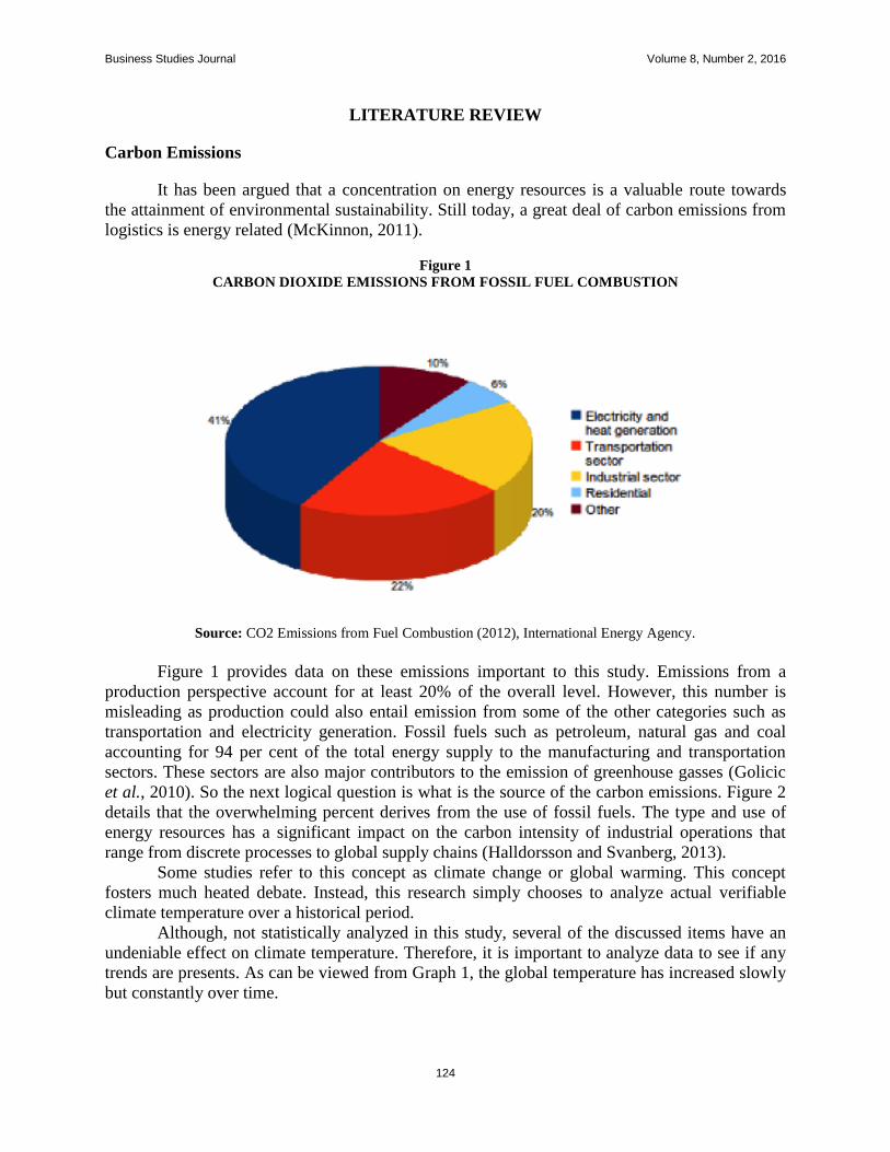
Business Studies Journal Volume 8, Number 2, 2016
124
LITERATURE REVIEW
Carbon Emissions
It has been argued that a concentration on energy resources is a valuable route towards
the attainment of environmental sustainability. Still today, a great deal of carbon emissions from
logistics is energy related (McKinnon, 2011).
Figure 1
CARBON DIOXIDE EMISSIONS FROM FOSSIL FUEL COMBUSTION
Source: CO2 Emissions from Fuel Combustion (2012), International Energy Agency.
Figure 1 provides data on these emissions important to this study. Emissions from a
production perspective account for at least 20% of the overall level. However, this number is
misleading as production could also entail emission from some of the other categories such as
transportation and electricity generation. Fossil fuels such as petroleum, natural gas and coal
accounting for 94 per cent of the total energy supply to the manufacturing and transportation
sectors. These sectors are also major contributors to the emission of greenhouse gasses (Golicic
et al., 2010). So the next logical question is what is the source of the carbon emissions. Figure 2
details that the overwhelming percent derives from the use of fossil fuels. The type and use of
energy resources has a significant impact on the carbon intensity of industrial operations that
range from discrete processes to global supply chains (Halldorsson and Svanberg, 2013).
Some studies refer to this concept as climate change or global warming. This concept
fosters much heated debate. Instead, this research simply chooses to analyze actual verifiable
climate temperature over a historical period.
Although, not statistically analyzed in this study, several of the discussed items have an
undeniable effect on climate temperature. Therefore, it is important to analyze data to see if any
trends are presents. As can be viewed from Graph 1, the global temperature has increased slowly
but constantly over time.

Business Studies Journal Volume 8, Number 2, 2016
125
Figure 2
HUMAN SOURCES OF CARBON DIOXIDE
Source: Le Quéré, C. et al. (2013). The global carbon budget 1959-2011.
2.2 Climate Temperature
Graph 1
GLOBAL TEMPERATURES OVER A 122-YEAR PERIOD
Source: NASA 2002 surface temperature summation.

Business Studies Journal Volume 8, Number 2, 2016
126
Energy
Production of energy is the process of (Halldorsson and Svanberg, 2013). Energy is a
source of power that is produced through using different technologies such as solar, wind, or
combustion. Various energy carriers (biomass, crude oil, sunlight, coal, natural gas, wind)
transform this energy to a consumable form of (electricity, vehicle fuel, heat, etc.…). This paper
will not delve into specifics on coal vs. solar for instance as much has already been written on
each of the various energy methods.
Figure 3 breaks down the means by which the U.S. generates electricity for consumption.
It becomes clear fossil fuels dominant the current used source and renewable means are a
negligible 13.2%. Table 1 provides a means of comparison to benchmark the U.S. with other
countries in this regard. While the U.S. is not quite the largest user of fossil fuels, percent-wise, it
is far from the leader or even in the middle of the pack. Recent evidence ranks "reduced costs
due to energy efficiency" as the second highest potential "sustainability benefit" for
organizations, only superseded by improved brand reputation (Haanes et al., 2011). However,
this sole work needs supporting research to confirm results. Therefore:
Hypothesis 1 As energy efficiency (EE) improves, overall, total costs (TC) will be reduced.
An examination of respondents will also try and confirm if brand reputation is indeed
regarded as having the highest “potential” over reduced costs. Clearly, as the U.S is economic
superpower, there is room for industry improvement. As a supplemental, Appendix A, is
attached to show a state-by-state comparison. This will allow, among other things, a means to
determine where efforts could begin.
Figure 3
U.S. 2014 ELECTRICITY GENERATION BY TYPE
Source: U.S. Energy and Information Administration. 2016.
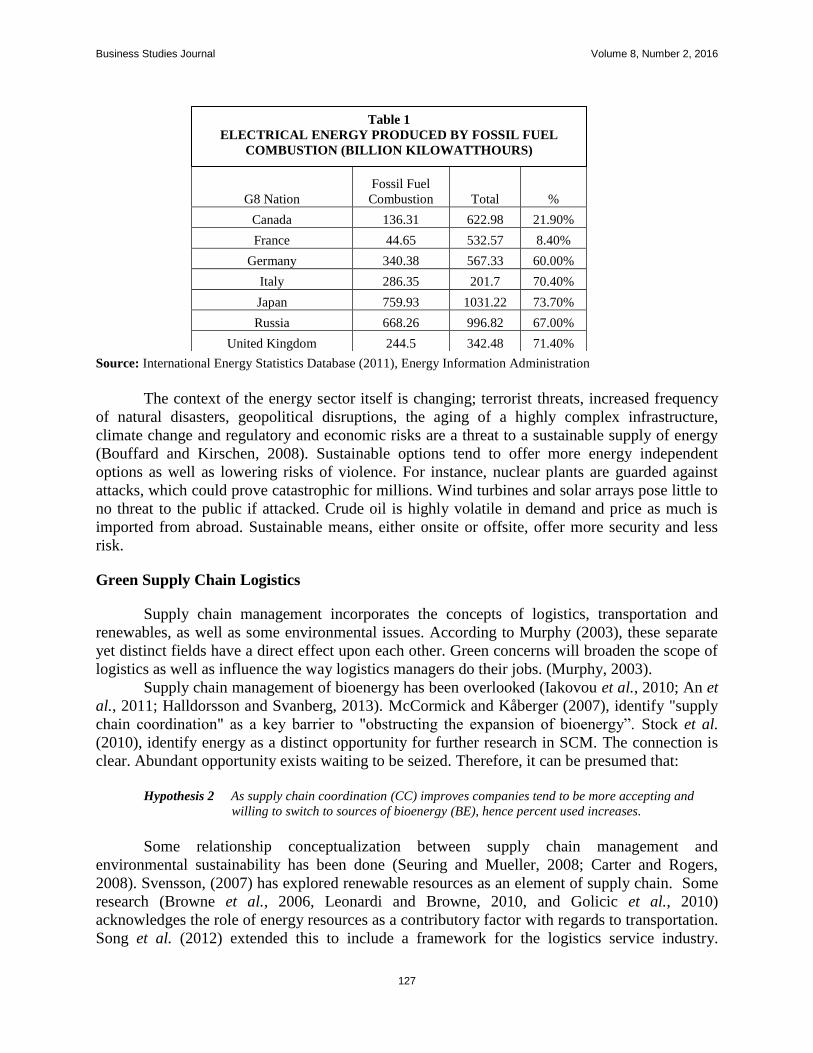
Business Studies Journal Volume 8, Number 2, 2016
127
Source: International Energy Statistics Database (2011), Energy Information Administration
The context of the energy sector itself is changing; terrorist threats, increased frequency
of natural disasters, geopolitical disruptions, the aging of a highly complex infrastructure,
climate change and regulatory and economic risks are a threat to a sustainable supply of energy
(Bouffard and Kirschen, 2008). Sustainable options tend to offer more energy independent
options as well as lowering risks of violence. For instance, nuclear plants are guarded against
attacks, which could prove catastrophic for millions. Wind turbines and solar arrays pose little to
no threat to the public if attacked. Crude oil is highly volatile in demand and price as much is
imported from abroad. Sustainable means, either onsite or offsite, offer more security and less
risk.
Green Supply Chain Logistics
Supply chain management incorporates the concepts of logistics, transportation and
renewables, as well as some environmental issues. According to Murphy (2003), these separate
yet distinct fields have a direct effect upon each other. Green concerns will broaden the scope of
logistics as well as influence the way logistics managers do their jobs. (Murphy, 2003).
Supply chain management of bioenergy has been overlooked (Iakovou et al., 2010; An et
al., 2011; Halldorsson and Svanberg, 2013). McCormick and Kåberger (2007), identify "supply
chain coordination" as a key barrier to "obstructing the expansion of bioenergy”. Stock et al.
(2010), identify energy as a distinct opportunity for further research in SCM. The connection is
clear. Abundant opportunity exists waiting to be seized. Therefore, it can be presumed that:
Hypothesis 2 As supply chain coordination (CC) improves companies tend to be more accepting and
willing to switch to sources of bioenergy (BE), hence percent used increases.
Some relationship conceptualization between supply chain management and
environmental sustainability has been done (Seuring and Mueller, 2008; Carter and Rogers,
2008). Svensson, (2007) has explored renewable resources as an element of supply chain. Some
research (Browne et al., 2006, Leonardi and Browne, 2010, and Golicic et al., 2010)
acknowledges the role of energy resources as a contributory factor with regards to transportation.
Song et al. (2012) extended this to include a framework for the logistics service industry.
G8 Nation
Fossil Fuel
Combustion Total %
Canada 136.31 622.98 21.90%
France 44.65 532.57 8.40%
Germany 340.38 567.33 60.00%
Italy 286.35 201.7 70.40%
Japan 759.93 1031.22 73.70%
Russia 668.26 996.82 67.00%
United Kingdom 244.5 342.48 71.40%
Table 1
ELECTRICAL ENERGY PRODUCED BY FOSSIL FUEL
COMBUSTION (BILLION KILOWATTHOURS)

Business Studies Journal Volume 8, Number 2, 2016
128
Although some research has begun in this broad field, it is far from abundant or sufficient. The
challenges of energy supply chains vary, depending on technology and mode of energy
production (solar, biomass, wind, water).
With current oil (energy) volatility, finite supplies, and emerging technologies, the
present is not only a feasible time but an optimal one for a transition to more sustainable
methods. Many of the producers of green technology, such as Toyota, “have failed to recognize
the mass-market appeal of their vehicles and its significant contribution to a cleaner environment
and to less dependency on oil” (Bockmam, 2009). Organizations realize that a strong supporting
logistics function is an important organizational offering from both the commercial and the
consumer perspective (Sarkis, 2004).
Competitive Advantages
Firms can increase their competitive advantage as a result of a stronger triple bottom line,
(composed of social, economic, and environmental issues or people, planet, and profit)
propositions are created from a natural-resource-based view of the firm perspective that is
supported using accounting theory, management strategy, green logistics and supply chain
literatures (Markley 2007). Other countries have begun realizing the importance of green
logistics and energy (Jiang, 2007). Research in this area could indeed help the entire country and
world but, more importantly, it would pave a way to improve local communities and economies.
Hence, additional studies in these areas would be a natural extension of existing programs for the
emerging field of green logistics. Take for instance a study done by Ranta and Korpinen (2011),
in which they found using local fuels actually lowered supply costs as well as making supply
more sustainable. This proved to be an ideal situation. So,
Hypothesis 3 As the overall percent of local fuels (LF) used increases, supply costs (SC) will decrease.
Hypothesis 4 As the overall percent of local fuels (LF) used increases, overall sustainability (ST)
improves (meaning sources of fuels tend to be green).
Rogers et al. (2007) conclude that accessibility of petroleum-based fuels still makes these
economically feasible over alternative sources of energy, and such "access to plentiful and
inexpensive fuels has been an important part of building successful supply chains". Rogers et al.
(2007) further concluded that supply chains have been built on the assumption that "petroleum-
based fuel would be inexpensive and plentiful for a long time". Christopher (2010) stresses the
same urgency: "When many of today's supply chains were originally designed, the cost of oil
was a fraction of what it is today". Competitive advantage potentials not only exist, they are
becoming more easily created. This is due to numerous factors such as higher gasoline prices,
lower costs of alternate energy sources such as solar and wind, and governmental incentive
programs for “green” initiatives.
METHODOLOGY
Questionnaire Design and Measure
The survey item was designed to obtain responses on a five-point Likert scale. A score of
3 represents average. A score of 1 represents very poor while 2 being poor. A score of 4 is
classified as very good and 5 is excellent. Actual, quantifiable data is excruciating limited in this

Business Studies Journal Volume 8, Number 2, 2016
129
type field. This may be one reason more research in this area has not been previously done.
Therefore, perceptions of observed or suspected benefits were asked. This was one reason the
survey was sent to a tactical or strategic level manager, so they would have the expertise and
knowledge on which to draw upon for these type questions.
Questionnaires were emailed when there was an option to do so. The remaining surveys
were mailed via United State Postal Service (USPS) to the operational manager at each facility.
Each questionnaire included a self-addressed, postage paid return envelope.
Sampling and Data Collection
This study utilized primary data collection methods for sourcing. Data was collected from
various types of industries located in the United States, Mexico and Canada using the survey
instrument that was developed.
These individual companies’ emails addresses were collected through a few various
means. However, all came via the Internet. A partial list of the companies was found via Google
searches, and some from the website Kellysearch.com. Others were found through ThomasNet.
The combined population size is over two thousand companies. However, it was not, in all cases,
possible to know with certainty if a certain company was involved in environmentalism or
sustainability on any level. Therefore, some surveys may have been sent to companies who did
not respond due to an inability to answer.
A total of 1000 surveys were mailed to various firms throughout the United States,
Mexico and Canada. 128 surveys were returns. Fortunately, only 2 of the 128 were found to be
unusable. This brought the effective sample response rate to 12.6%. Other supply chain related
studies have found response rates typically to be much, much higher than 12.6% (Swink et al.,
2007; Devaraj et al., 2007; Koufteros et al., 2005; Rosenzweig et al., 2003). This may be due to
several factors, among them was no prior personal relationship with any of the firms being
surveyed and that no contact was made at any time via the telephone with any firms. This could
have potentially increased the viable response rate. If an answer was illegible, then that
questionnaire was added to the unusable stack.
Tables 2 and 3 show a profile of respondents as well as some brief demographic
descriptors. Approximately 75% of those who answered the survey were mid to upper
management, had more than 6 years’ experience, and possessed a Bachelor’s degree or higher.
Therefore, it is felt these individuals should be knowledgeable in regards to the information
asked of them, as was expected.

Business Studies Journal Volume 8, Number 2, 2016
130
Table 2
RESPONDENT CHARACTERISTICS
Position % of
respondents
Years
Experience
% of
respondents
Age
Group
% of
respondents
Highest
Education
Level
Completed
% of
respondents
Upper
Management 12.8 <5 years 5.9 <30 years 2.2
High
School 15.8
Mid
Management 62.5 6-10 years 30.5
30-39
years 22.6 Associates 7.7
Other 22.2 11-15
years 43.7
40-49
years 43.5 Bachelor 38.9
No response 2.5 16-20
years 10.7
50-59
years 22.6 Graduate 24.7
>21 years 6.8 >60 years 2.6 Post
Graduate 6.2
No
response 2.4
No
response 6.5 Other 2.9
No
response 3.8
Table 3
DEMOGRAPHIC PROFILE OF RESPONDING COMPANIES
Size of
Company
base on
labor force
% of
respondents
Size of
Company
base on
market
capital
% of
respondents
Region of
Responding
Company
% of
respondents
Company
Public or
Private
% of
respondents
<50 2.5 >$1M 0.4 Northeast 13.93 Public 43.7
50-100 13.8 $1-5M 6.2 Northwest 12.19 Private 46.8
100-200 32.5 $5-10M 9.4 Central 14.43 No
response 9.5
200-500 38.6 $10-25M 27.7 Southwest 14.93
>500 8.1 $25-100M 32.7 Southeast 12.69
No response 4.6 >$100M 18.9 Canada 31.34
No response 4.8 No response 0.5
Reliability and Validity
Confirmatory factor analysis (CFA) was used to test the latent variables. Confirmatory
factor analysis was chosen since it provides a more demanding testing of theory compared to that
of exploratory factor analysis (EFA), yet it extends the results generated from the EFA to those
presented in the measurement model. Also, CFA allows the researcher to evaluate a priori
relationships whereas EFA does not require a priori specifications for theorized relationships
prior to model testing. CFA permits the indicators to load only on certain pre-selected factors,
while EFA permits the data and statistical technique to determine the measurement model (Hair
et al., 1998).
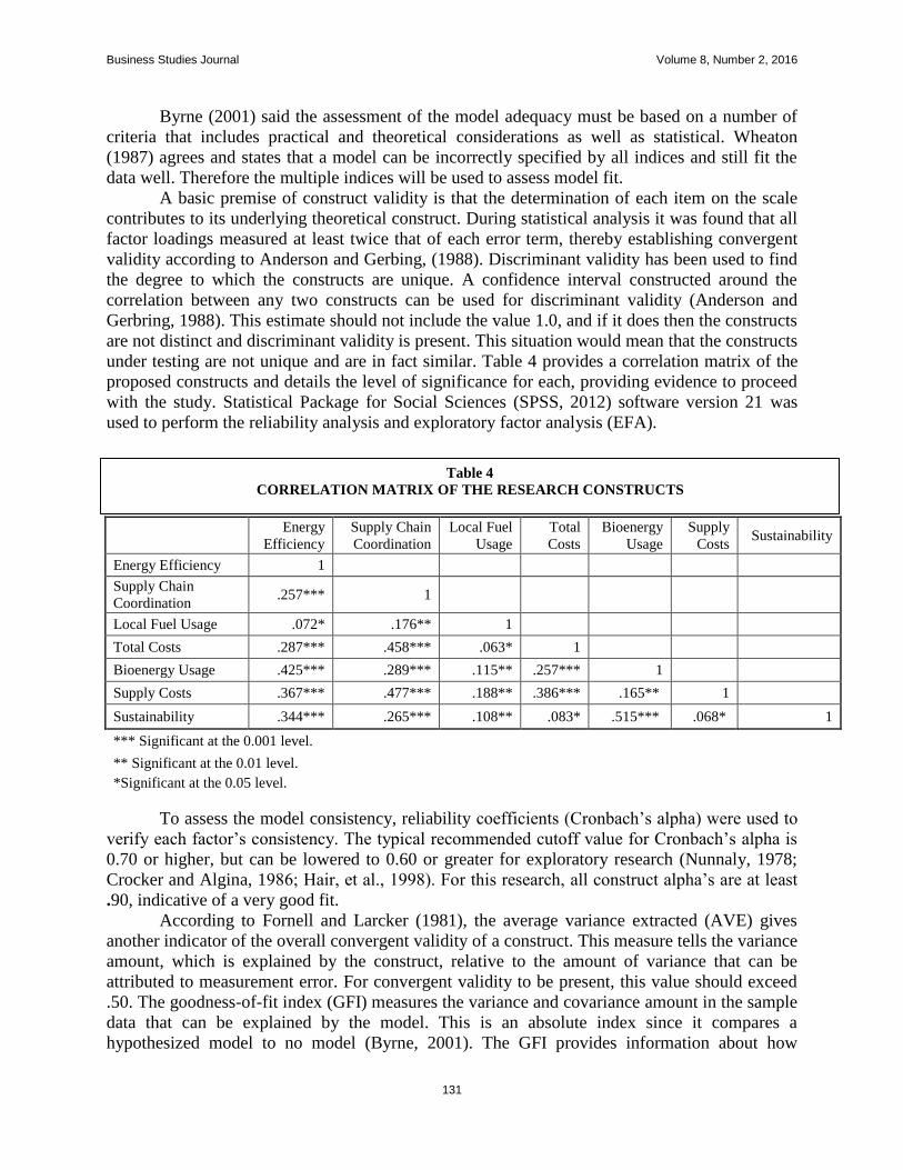
Business Studies Journal Volume 8, Number 2, 2016
131
Byrne (2001) said the assessment of the model adequacy must be based on a number of
criteria that includes practical and theoretical considerations as well as statistical. Wheaton
(1987) agrees and states that a model can be incorrectly specified by all indices and still fit the
data well. Therefore the multiple indices will be used to assess model fit.
A basic premise of construct validity is that the determination of each item on the scale
contributes to its underlying theoretical construct. During statistical analysis it was found that all
factor loadings measured at least twice that of each error term, thereby establishing convergent
validity according to Anderson and Gerbing, (1988). Discriminant validity has been used to find
the degree to which the constructs are unique. A confidence interval constructed around the
correlation between any two constructs can be used for discriminant validity (Anderson and
Gerbring, 1988). This estimate should not include the value 1.0, and if it does then the constructs
are not distinct and discriminant validity is present. This situation would mean that the constructs
under testing are not unique and are in fact similar. Table 4 provides a correlation matrix of the
proposed constructs and details the level of significance for each, providing evidence to proceed
with the study. Statistical Package for Social Sciences (SPSS, 2012) software version 21 was
used to perform the reliability analysis and exploratory factor analysis (EFA).
Energy
Efficiency
Supply Chain
Coordination
Local Fuel
Usage
Total
Costs
Bioenergy
Usage
Supply
Costs Sustainability
Energy Efficiency 1
Supply Chain
Coordination .257*** 1
Local Fuel Usage .072* .176** 1
Total Costs .287*** .458*** .063* 1
Bioenergy Usage .425*** .289*** .115** .257*** 1
Supply Costs .367*** .477*** .188** .386*** .165** 1
Sustainability .344*** .265*** .108** .083* .515*** .068* 1
*** Significant at the 0.001 level.
** Significant at the 0.01 level.
*Significant at the 0.05 level.
To assess the model consistency, reliability coefficients (Cronbach’s alpha) were used to
verify each factor’s consistency. The typical recommended cutoff value for Cronbach’s alpha is
0.70 or higher, but can be lowered to 0.60 or greater for exploratory research (Nunnaly, 1978;
Crocker and Algina, 1986; Hair, et al., 1998). For this research, all construct alpha’s are at least
.90, indicative of a very good fit.
According to Fornell and Larcker (1981), the average variance extracted (AVE) gives
another indicator of the overall convergent validity of a construct. This measure tells the variance
amount, which is explained by the construct, relative to the amount of variance that can be
attributed to measurement error. For convergent validity to be present, this value should exceed
.50. The goodness-of-fit index (GFI) measures the variance and covariance amount in the sample
data that can be explained by the model. This is an absolute index since it compares a
hypothesized model to no model (Byrne, 2001). The GFI provides information about how
Table 4
CORRELATION MATRIX OF THE RESEARCH CONSTRUCTS

Business Studies Journal Volume 8, Number 2, 2016
132
closely the models fitted compare to one of a perfect fit (Maruyama, 1998). GFI’s NFI’s, and
CFI’s should all be close to .9 for an indication of excellent fit.
Hair et al. (1998) tell that reliability determines the extent to which an observed manifest
variable measures the concept is supposed to measure. The composite reliability measure should
exceed .50 to be considered good. Average variance extracted (AVE) is one measure of overall
validity shown in the table. The AVE is defined as “the sum of squared loading of a scaled
divided by the number of items per scale (Fornell and Larcker, 1981). The AVE value should
exceed .5 to be considered a very good fit. Garver and Mentzer (1999) recommend using a root
mean square error of approximation (RMSEA) .8 or below. However, Hu and Bentler (1999) and
Browne and Cudeck (2003) provide evidence that the RMSEA must be .06 or below for an
acceptable level of fit. As evidenced by Table 5 all statistical finding are well within range for
good fit.
Energy
Efficiency
Supply
Chain
Coordination
Local
Fuel
Usage
Total
Costs
Bioenergy
Usage
Supply
Costs Sustainability
Goodness of Fit (GFI) 0.928 0.975 0.955 0.937 0.978 0.963 0.967
Root mean square
error of
approximation
(RMSEA) 0.058 0.045 0.048 0.052 0.054 0.049 0.05
Normed fit index
(NFI) 0.905 0.931 0.927 0.918 0.935 0.932 0.937
Comparative fit index
(CFI) 0.924 0.96 0.948 0.93 0.962 0.955 0.958
p-value 0.00464 0.00388 0.00435 0.00445 0.00371 0.00429 0.00315
Average Variance
Extracted (AVE) 0.688 0.714 0.735 0.77 0.695 0.73 0.795
Composite Reliability 0.9 0.96 0.93 0.91 0.96 0.94 0.95
Cronbach's Alpha 0.9195 0.9678 0.9348 0.9232 0.9715 0.9454 0.9472
Table 6 provides several goodness-of- fit statistics to judge how well the model explains
the observed data from the aspects of: absolute fit, incremental fit, and parsimonious fit (Tanaka,
1993; Maruyama, 1998). The absolute fit measures of GFI, AGFI, and the Normed chi-square
indicate a good fit of the model to the data (Bentler and Bonnet, 1980; Bagozzi and Yi, 1988).
Table 5
MODEL INDICES
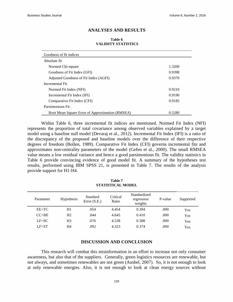
Business Studies Journal Volume 8, Number 2, 2016
133
ANALYSES AND RESULTS
Table 6
VALIDITY STATISTICS
Goodness of fit indices
Absolute fit
Normed Chi-square 1.3200
Goodness of Fit Index (GFI) 0.9398
Adjusted Goodness of Fit Index (AGFI) 0.9370
Incremental Fit
Normed Fit Index (NFI) 0.9210
Incremental Fit Index (IFI) 0.9190
Comparative Fit Index (CFI) 0.9185
Parsimonious Fit
Root Mean Square Error of Approximation (RMSEA) 0.5280
Within Table 6, three incremental fit indices are mentioned. Normed Fit Index (NFI)
represents the proportion of total covariance among observed variables explained by a target
model using a baseline null model (Devaraj et al., 2012). Incremental Fit Index (IFI) is a ratio of
the discrepancy of the proposed and baseline models over the difference of their respective
degrees of freedom (Bollen, 1989). Comparative Fit Index (CFI) governs incremental fits and
approximates non-centrality parameters of the model (Gefen et al., 2000). The small RMSEA
value means a low residual variance and hence a good parsimonious fit. The validity statistics in
Table 6 provide convincing evidence of good model fit. A summary of the hypotheses test
results, performed using IBM SPSS 21, is presented in Table 7. The results of the analysis
provide support for H1-H4.
Table 7
STATISTICAL MODEL
Parameter Hypothesis Standard
Error (S.E.)
Critical
Ratio
Standardized
regression
weights
P-value Supported
EE>TC H1 .054 4.454 0.394 .000 Yes
CC>BE H2 .044 4.645 0.410 .000 Yes
LF>SC H3 .076 4.538 0.388 .000 Yes
LF>ST H4 .092 4.323 0.374 .000 Yes
DISCUSSION AND CONCLUSION
This research will combat this misinformation in an effort to increase not only consumer
awareness, but also that of the suppliers. Generally, green logistics resources are renewable, but
not always, and sometimes renewables are not green (Ausbel, 2007). So, it is not enough to look
at only renewable energies. Also, it is not enough to look at clean energy sources without

Business Studies Journal Volume 8, Number 2, 2016
134
applications. Once green methods are identified as viable, there should be a seamless transition
to implement these methods into society.
Rao (2004), found that education of the public can prove to be beneficial with regard to
change. He asserts that the public often, through informal channels, exerts pressure and influence
on the polluters of the environment. A recent report from the BLS (2014), Figure 4, provides
hope of moving to more environmental and sustainable energy means. The study finds solar use
increasing at 200% and other “green” methods showing positive gains, although much smaller.
Although renewable resources have been referred to in a positive vein in this paper,
further understanding of these in a SCM context must consider the negative effects these may
have on the wider system, such as noise, visual intrusion, health and safety, water pollution, and
traffic generation (Allen et al., 1998). Another issue that must be dealt with is supply risk, in
which a key component is dependency
Stock et al. (2010), identify energy as a distinct opportunity for further research in SCM.
This reinforces this papers findings that present day pollution, carbon emissions, and climate
temperatures are increasing while use of fossils fuels is increasing in volume, if not percent.
Therefore, energy remains an elusive opportunity for advancement of “green” ideals that will be
environmentally helpful and arguably productively and financially beneficial to industry.
Future studies could focus on many different aspects. One of which might be climate
temperature. According to Graph 1, it appears that in the 1970’s this temperature began to
sharply increase and continues to do so. Investigation could be done to provide a solid corollary
between greening of energy and production, sustainability, environmentalism, etc… and
lowering of the climate temperature.
Figure 4
U.S. ELECTRIC POWER SECTOR JOBS IN GENERATION BY ENERGY SOURCE (JAN 2011-JUNE
2014)
Source: Bureau of Labor Statistics (BLS) Quarterly Census of Employment and Wages

Business Studies Journal Volume 8, Number 2, 2016
135
REFERENCES
Allen, J., Browne, M., Hunter, A., Biyd, J. and Palmer, H. (1998). Logistics management and costs of biomass fuel
Supply. International Journal of Physical Distribution & Logistics Management, 28(6), 463-477.
An, H., Wilhelm, W.E. and Searcy, S.W. (2011). Biofuel and petroleum-based fuel supply chain research: a
literature review. Biomass and Bioenergy, 35(9), 3763-3774.
Anderson, G. W., & Gerbing, D.W. (1988). Structural equation modeling in practice: A review and recommend two-
step approach. Psychological Bulletin, 103(3), 411-423.
Ausbel, Jesse H. (2007). Renewable and nuclear heresies. International Journal of Nuclear Governance, Economy
and Ecology, 1(3), 229-243.
Bagozzi, R. P., & Yi, Y. (1988). On the evaluation of structural equation models. Academy of Marketing Science
Journal, 16(1), 74-94.
Bentler, P.M., & Bonnet, D.G. (1980). Significance tests and goodness of fit in the analysis of covariant structures.
Psychological Bulletin, 88(3), 588–606. BLS (2014). Bureau of Labor Statistics Quarterly
Census of Employment and Wages.
http://www.bls.gov/cew/data.htm
Bockmam, Shel, Razzouk, Nabil, Sirotnik, Barbara (2009). Going Green - From Left to Center Stage: An Empirical
Perspective. Journal of American Academy of Business, 14(2), 8-9.
Bollen, K. A. (1989). A new increment fit index for general structural equation models. Sociological Methods and
Research, 17(3), 303-316.
Bouffard, F. and Kirschen, D.S. (2008). Centralised and distributed electricity systems. Energy Policy, 36(12), 4504-
4508.
Browne, M., Allen, J. and Rizet, C. (2006). Assessing transport energy consumption in two product supply chains.
International Journal of Logistics: Research & Applications, 9(3), 237-252.
Browne, M., & Cudeck, R., (2003). Alternative ways of assessing model fit. In: Bollen, K.A., Long, J.S. (Eds.),
Testing Structural Equation Models. Sage Publications, London, U.K.
Byrne, B.M. (2001). Structural equation modeling with AMOS: Basic concepts, applications, and programming.
Mahwah, NJ: Lawrence Erlbaum Associates.
Carter, C.R. and Rogers, D.S. (2008). A framework of sustainable supply chain management: moving toward new
Theory. International Journal of Physical Distribution & Logistics Management, 38(5), 360-387.
Christopher, M. (2010). Logistics and Supply Chain Management: Creating Value-Added Networks, Financial
Times/Prentice Hall, Harlow.
Crocker, L., & Algina, L. (1986). Introduction to classical and modern test theory. Fort Worth, TX, Harcourt,
Brace, Jovanovich.
Devaraj, S., Krajewski, L., & Wei, J. C. (2007). Impact of eBusiness technologies on operational performance: The
role of production information integration in the supply chain. Journal of Operations Management, 25(6),
1199-1216.
Devaraj, S., Vaidyanathan, G., & Mishra, A. N. (2012). Effect of purchase volume flexibility and purchase mix
flexibility on e-procurement performance: An analysis of two perspectives. Journal of Operations
Management, 30(7-8), 509.
Energy Information Administration (2011). International Energy Statistics Database.
Fornell, C., & Larcker, D.F. (1981). Evaluating structural equation models with observable variables and
measurement error. Journal of Marketing Research 18(1), 39-50.
Garver, M. S., & Mentzer, J. T. (1999). Logistics research methods: Employing structural equation modeling to test
for construct validity. Journal of Business Logistics, 20(1), 33-57.
Gefen, D., Straub, D.W., & Boudreau, M.C. (2000). Structural equation modeling and regression: guidelines for
research practice. Communications of AIS, 4 (7), 71–78.
Golicic, S., Boerstler, C. and Ellram, L.M. (2010). Greening transportation in the supply chain. MIT Sloan
Management Review, 51(2), 47-55.
Haanes, K., Balagopal, B., Arthur, D., Kong, M.T., Velken, I., Kruschwitz, N. and Hopkins, M.S. (2011). First
Look: The Second Annual Sustainability & Innovation Survey. MIT Sloan Management Review, 52(2), 77-
83.
Halldórsson, Á., & Svanberg, M. (2013). Energy resources: Trajectories for supply chain management. Supply
Chain Management, 18(1), 66-73.

Business Studies Journal Volume 8, Number 2, 2016
136
Hair, J., J.F., Anderson, R.E., Tatham, R.L., & Black, W.C. (1998). Multivariate Data Analysis. Upper Saddle
River, NJ, Prentice Hall.
Iakovou, E., Karagiannidis, A., Vlachos, D., Toka, A. and Malamakis, A. (2010). Waste biomass-to-energy supply
chain management: a critical synthesis. Waste Management, 30(10) 1860-1870.
International Energy Agency (2012). CO2 Emissions from Fuel Combustion.
Jiang, Kejun, Zhu, Songli, Shrestha, Ram M.(2007). Analysis of policy options for promotion of clean and energy
efficient technologies in the transport sector in Beijing. International Journal of Environment & Pollution.
30(1) 59.
Koufteros, X., Vonderembse, M., & Jayaram, J. (2005). Internal and external integration for product development:
The contingency effects of uncertainty, equivocality, and platform strategy. Decision Sciences, 36(1), 97-
133.
Leonardi, J. and Browne, M. (2010). A method for assessing the carbon footprint of maritime freight transport:
European case study and results. International Journal of Logistics Research and Applications, 13(5), 349-
358.
Markley, Melissa J., Davis, Lenita (2007). Exploring future competitive advantage through sustainable supply
chains. International Journal of Physical Distribution & Logistics Management. 37(9), 763.
Maruyama, G.M., (1998). Basics of Structural Equation Modeling. Sage Publishers, Thousand Oaks, CA.
McCormick, K. and Kåberger, T. (2007). Key barriers for bioenergy in Europe: economic conditions, know-how
and institutional capacity, and supply chain co-ordination", Biomass and Bioenergy, 31(7), 443-452.
McKinnon, A.C. (2011). Developing a decarbonisation strategy for logistics, in Waterson, B. (Ed.), Proceedings of
the 16th Annual Logistics Research Network Conference, “Smarter Logistics: Innovation for Efficiency,
Performance and Austerity", held 7-9 September 2011 at the University of Southampton, Southampton.
Moore, Kelly, Neu Gebauer, Romain, Lurmann, Fred, Hall, Jane (2008). Ambient Ozone Concentrations Cause
Increased Hospitalizations for Asthma in Children: An 18-Year Study in Southern California.
Environmental Health Perspectives. 116(8), 1063.
Murphy, Paul R., Poist, Richard F. (2003). Green perspectives and practices: A comparative logistics study. Supply
Chain Management. 8(2), 122.
NASA (2002). Surface temperature summation. http://data.giss.nasa.gov/gistemp/2002/
NEI (2015). Nuclear Energy Institute. State Electricity Generation Fuel Shares.
Nunnaly, J. C. (1978). Psychometric Theory. New York, McGraw-Hill.
Quéré, C. Le, et al. The global carbon budget 1959–2011. Earth System Science Data, 5.1(2013), 165-185.
Ranta, T. and Korpinen, O.J. (2011). How to analyse and maximise the forest fuel supply availability to power
plants in Eastern Finland. Biomass and Bioenergy, 35(5), 1841-1850.
Rao, P. (2004). Greening production: A south-east asian experience. International Journal of Operations &
Production Management, 24(3), 289-320.
Rogers, Z., Kelly, T.G., Rogers, D.S. and Carter, C.R. (2007). Alternative fuels: are they achievable? International
Journal of Logistics: Research & Application, 10(3), 269-82.
Rosenzweig, E. D., Roth, A. V., & Dean, James W., Jr. (2003). The influence of an integration strategy on
competitive capabilities and business performance: An exploratory study of consumer products
manufacturers. Journal of Operations Management, 21(4), 437-456.
Sarkis, Joseph, Meade, Laura M., Talluri, Srivnas (2004). E-logistics and the natural environment. Supply Chain
Management. 9(3/4), 303.
Seuring, S. and Mueller, M. (2008). From a literature review to a conceptual framework for sustainable supply chain
management. Journal of Cleaner Production, 16(15), 1699-1710.
Song, M., Wang, S., Jiang, Z., Yang, J. and Wang, Y. (2012). Will environmental logistics be promoted by changing
industrial structure? A quantitative analysis from 1978 to 2007 in China", Supply Chain Management: An
International Journal, 17(1), 5-14.
SPSS, (2012). IBM Corp. IBM SPSS Statistics for Macintosh, Version 21.0. Armonk, NY: IBM Corp.
Stock, J.R., Boyer, S.L. and Harmon, T. (2010). Research opportunities in supply chain management. Journal of the
Academy of Marketing Science, 38, 32-41.
Svensson, G. (2007). Aspects of sustainable supply chain management (SSCM): conceptual framework and
empirical example. Supply Chain Management: An International Journal, 12(4), 262-266.
Swink, M., Narasimhan, R., & Wang, C. (2007). Managing beyond the factory walls: Effects of four types of
strategic integration on manufacturing plant performance. Journal of Operations Management, 25(1), 148-
164.

Business Studies Journal Volume 8, Number 2, 2016
137
Tanaka, J.S. (1993). Multifaceted conceptions of fit in structural equation models. In: Bollen, K.A., Long, J.S.
(Eds.), Testing Structural Equation Models. Sage Publishers, Newbury Park, CA.
U.S. Energy and Information Administration (2016).
http://www.eia.gov/electricity/monthly/epm_table_grapher.cfm?t=epmt_1_01
Wheaton, B. (1987). Assessment of fit in overidentified models with latent variables. Sociological Methods &
Research 12, 118-154.

Business Studies Journal Volume 8, Number 2, 2016
138
Appendix A
PERCENT ELECTRICITY GENERATED WITHIN THE BORDERS OF EACH STATE
State Nuclear Coal Natural
Gas Petroleum Hydro Geothermal Solar/PV Wind Biomass/Other
Alabama 27.5 31.5 32.2 0.1 6.5 0 0 0 2.2
Alaska 0 9.2 49.3 12.8 24.9 0 0 2.5 1.3
Arizona 28.8 38 24.3 0.1 5.5 0 2.8 0.4 0.2
Arkansas 23.5 53.9 15.7 0 4.2 0 0 0 2.6
California 8.6 0.4 60.5 0 8.2 6.4 5 7 3.9
Colorado 0 60.3 22.5 0 2.8 0 0.5 13.6 0.2
Connecticut 47.1 2.5 43.6 1.5 1.1 0 0 0 4.2
Delaware 0 11.3 84.9 2.1 0 0 0.8 0.1 0.8
District of
Columbia 0 0 100 0 0 0 0 0 0
Florida 12.1 22.6 61.6 0.2 0.1 0 0.1 0 3.4
Georgia 25.9 36.1 32.4 0.1 2 0 0.1 0 3.4
Hawaii 0 15.1 0.3 69.4 0.8 2.5 0.5 5.9 5.4
Idaho 0 0.6 16.4 0 60.4 0.3 0 18.3 3.9
Illinois 48.4 43.2 2.9 0 0.1 0 0 5 0.5
Indiana 0 83.3 12.4 0.1 0.3 0 0.1 3 0.7
Iowa 7.3 60 2.6 0.1 1.3 0 0 28.5 0.3
Kansas 17.1 57.5 3.5 0.1 0 0 0 21.7 0.1
Kentucky 0 93.2 2.7 0.1 3.4 0 0 0 0.6
Louisiana 16.6 23.4 55.8 0 1 0 0 0 3
Maine 0 0.6 33.7 2.3 25 0 0 8.3 30.1
Maryland 37.7 46.3 6.9 1.3 4.3 0 0.3 0.9 2.4
Massachusetts 18.5 9.4 58.5 3.2 1.6 0 1.3 0.7 6.7
Michigan 29.5 51 11.9 0.1 0.7 0 0 3.7 3
Minnesota 22.4 50.2 6.8 0.1 0.9 0 0 15.9 3.6
Mississippi 18.5 19.6 59.2 0 0 0 0 0 2.7
Missouri 10.5 82.6 4.5 0.1 0.8 0 0 1.3 0.1
Montana 0 53.7 1.8 0.1 37.1 0 0 6.5 0.9
Nebraska 25.5 63.2 1.1 0.1 3 0 0 6.9 0.2
Nevada 0 18.1 63.1 0 6.7 8.3 2.8 0.8 0.1
New Hampshire 51.9 6.7 22.4 1.5 6.9 0 0 2.1 8.4
New Jersey 46.7 3.8 45.7 0.7 -0.3 0 1 0 2.3
New Mexico 0 63.4 27.1 0.2 0.4 0.1 1.7 7 0.1
New York 31.6 3.4 39.6 1.6 18.4 0 0.1 2.9 2.5
North Carolina 31.8 38.7 22.4 0.3 4 0 0.7 0 2.1
North Dakota 0 75.1 0.2 0.1 7 0 0 17.6 0.1
Ohio 12.1 67.7 18.2 0.2 0.3 0 0 0.9 0.6
Oklahoma 0 42.6 38 0 2 0 0 16.9 0.5
Oregon 0 5.3 21.2 0 58.5 0.3 0.1 12.7 1.9
Pennsylvania 35.5 36.2 23.9 0.3 1 0 0 1.6 1.5
Rhode Island 0 0 94.7 1.5 0.1 0 0.3 0.1 3.3
South Carolina 54 29.8 11.6 0.3 2 0 0 0 2.3
South Dakota 0 23.3 3.6 0.1 47.7 0 0 25.3 0
Tennessee 34.5 44.7 7.8 0.2 11.3 0 0 0.1 1.3
Texas 9 33.9 47.3 0 0.1 0 0.1 9 0.5
Utah 0 76.3 19 0.1 1.5 1.2 0 1.5 0.4
Vermont 72.3 0 0 0.2 16.1 0 0.4 4.4 6.6
Virginia 39.1 27 27 1.5 0 0 0 0 5.5
Washington 8.2 5.8 9.8 0 68.2 0 0 6.3 1.7
West Virginia 0 95.5 0.8 0.2 1.7 0 0 1.8 0
Wisconsin 15.5 62.3 13.2 0.1 3.4 0 0 2.6 2.8
Wyoming 0 87.7 1.6 0.1 1.7 0 0 8.9 0
Source: ABB Velocity Suite / Energy Information Administration. 2015

Business Studies Journal Volume 8, Number 2, 2016
139
ACCEPTABLE CHEATING BEHAVIORS?
Wendy C. Bailey, Troy University
S. Scott Bailey, Troy University
Connie Nott, Troy University
ABSTRACT
The investigation of academic dishonesty is timely, relevant and important to the global
business environment. There appears to be a link between acceptance of academic dishonesty
and ethical business decisions. Student attitudes towards academic dishonesty have been widely
studied across cultures in the last decade. International (Vietnamese) and domestic students
differ in their acceptance of specific forms of academic dishonesty. A total of 621 business
students responded to our survey. Respondents were either domestic or international and
graduate or undergraduate students. They responded to five statements and two questions about
academic dishonesty. Analysis of contingency tables indicated that international and
undergraduate students a higher acceptance for specific forms of cheating and that there is more
difference by gender among the international students.
INTRODUCTION
Business student cheating conjures up deep concerns since business leaders have been
known to act unethically (Smyth, Davis, and Knoncke, 2009). Chapman and Lipton (2004) refer
to cheating as a “widespread, insidious and global problem”. “There is an increased need for
business schools to address academic dishonesty because what students learn as acceptable
behavior in the classroom impacts their expectations of what is acceptable professionally.” Iyer
and Eastman (2006 p. 102). Obviously, academic dishonesty has importance far beyond the
academic setting and is being researched because of its global importance.
This study addresses the gap identified by Lupton, Chapman and Weiss (2000 p. 232)
when they stated “To date, there is little cross national cheating research”. Lin and Wen (2007)
also mention that more studies of Asian students are needed, since Asians are participating in the
workforce and a propensity to cheat could carry on into their careers.
We add to the literature on academic dishonesty and on cross national differences as well
as differences by class level and gender. We report on the acceptance level of specific forms of
academic dishonesty by international students, domestic students, graduate and undergraduate
students. Comparisons of male and female acceptance levels add to the gender literature on this
topic. A total of 621 students from one US public university responded to identical self-reported
statements and questions in English. There were 237 graduate students and 379 undergraduate
students. Of these, 217 were in international classes and 399 were in domestic classes, while 356
were female and 254 were male.
Business Studies Journal Volume 8, Number 2, 2016
140
LITERATURE REVIEW
Three broad research topics are relevant to this topic, academic dishonesty: 1) gender
differences, 2) international and domestic differences and 3) undergraduate and graduate student
differences.
Gender differences were explored in the late 20th
century primarily in the United States.
Earlier studies during this period seemed to indicate that there were gender differences, while
later studies (possibly as women participated more in many activities outside the home) showed
fewer statistically significant differences between the male and female perceptions of academic
dishonesty. Early conjecture by several authors raised several possible explanations for the
reported gender differences; the most common was attributed to variations in the male and
female socialization process. More recent studies demonstrate a convergence in attitude, possibly
because the academic environment is equalizing for men and women.
“Gender differences have been widely studied, but results are mixed as to whether there
truly are differences between men and women due to sex socialization” (Bailey and Bailey,
2011). The two articles by Bailey and Bailey (2011) include a detailed discussion of 20th
century
literature relating to gender differences as well as a more comprehensive summary of several
early 21st century international studies.
Lupton, Chapman and Weiss (2000) reported doing an extensive literature search on
cross national cheating research. There were only three articles that included international
comparisons. Since 2001 there has been increasing interest in how students from different
cultures view academic dishonesty. The three articles reported here are representative of wide
spread interest in international attitudes and comparisons.
Research by Jurdi, Hage and Chow (2011) surveyed 321 students in a Canadian
university in 2007, but disagreed with the previous discussions based on gender and age as
subgroups.
Chapman and Lipton (2004) focused on cross national differences in beliefs about
cheating when they compared US and Hong Kong students. They surveyed 443 US students and
622 Hong Kong students.
Lupton, Chapman and Weiss (2000) compared attitudes, perceptions and tendencies
toward cheating between undergraduate business students. They surveyed 443 US students and
192 students in Poland.
Lin and Wen (2007) document the results from a 2068 Taiwanese students surveyed on
four domains of academic dishonesty.
Iyer and Eastman’s (2006) article contained a comprehensive literature review on studies
comparing responses to academic dishonesty questions between business and non-business
students. They summarized multiple authors as finding that “younger, immature students cheat
more than do older, mature students; juniors and seniors cheat less than do freshmen or
sophomores; older students are more likely to view scenarios of academic dishonesty as serious
offenses; the ethics of graduate business students are similar to those of undergraduates, despite
graduate students perceiving themselves as more ethical than undergraduates.” (Bailey, Bailey
and Nott, 2014).
Rakovski and Levy (2007) found that graduate students were less likely than
undergraduates to participate in cheating. Iyer and Eastman (2006) also reported lower self-
reported cheating among graduate students. In addition they found no support for the hypothesis
that non-business students engage in lower levels of academic dishonesty than business students.

Business Studies Journal Volume 8, Number 2, 2016
141
This study adds to the literature on academic dishonesty in three areas. Our contingency
table analysis of the survey responses show significant differences in students in different
countries, in different levels of class work and of different genders.
METHODOLOGY
All students surveyed were attending classes at a single university in the United States
(domestic) or in Vietnam (international). The students were attending undergraduate or graduate
business classes. Table 1 shows the level of class work and the gender breakdown of the students
surveyed.
Table 1
DESCRIPTION OF SAMPLE RESPONDENTS
All Nationality Domestic International All students
surveyed
621 399 217
Undergraduates 379 187 192 Graduates 237 212 25 Males 254 158 96 Females 356 239 117
The survey had two parts. The first set of statements portrayed an academic situation
where another student was cheating on an exam using prohibited notes. The analysis of the
student responses to these five statements are reported in “International Students Do View
Cheating Differently” (Bailey, Bailey and Nott, 2014).
The two additional questions on the survey were: 1. Which of the following behaviors do you personally feel is acceptable and shouldn't constitute an academic
honesty violation? (Check all that apply).
2. Which of the following do you feel you might do if you felt there would be no legal or academic repercussions
from it? (Check all that apply).
The possible responses to these two questions were: 1. Copying short passages or a few sentences from a book, periodical, or the internet without providing a citation
2. Copying short passages or a few sentences from a book, periodical, or the internet and providing a citation, but
not using quotation marks
3. Giving a friend or acquaintance hints about what is included on an exam that you took already but they haven't
taken yet
4. Giving a friend or acquaintance copies of questions which were included on an exam that you took already but
they haven't taken yet
5. Taking an exam for another person
6. Using notes on an exam when you are not supposed to
7. Asking a classmate for an answer on an assignment or exam
8. Copying an answer from another classmate without them knowing about it
9. Turning in copies of solutions you found on the internet for solved problems as your own
10. Using a published test bank or instructor's manual to take tests or do graded homework
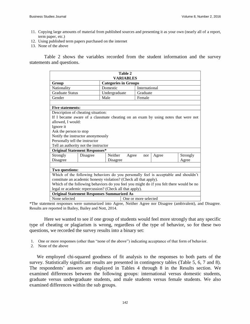
Business Studies Journal Volume 8, Number 2, 2016
142
11. Copying large amounts of material from published sources and presenting it as your own (nearly all of a report,
term paper, etc.)
12. Using published term papers purchased on the internet
13. None of the above
Table 2 shows the variables recorded from the student information and the survey
statements and questions.
Table 2
VARIABLES
Group Categories in Groups
Nationality Domestic International
Graduate Status Undergraduate Graduate
Gender Male Female
Five statements:
Description of cheating situation:
If I became aware of a classmate cheating on an exam by using notes that were not
allowed, I would:
1. Ignore it
2. Ask the person to stop
3. Notify the instructor anonymously
4. Personally tell the instructor
5. Tell an authority not the instructor
Original Statement Responses*
Strongly
Disagree
Disagree Neither Agree nor
Disagree
Agree Strongly
Agree
Two questions:
1. Which of the following behaviors do you personally feel is acceptable and shouldn’t
constitute an academic honesty violation? (Check all that apply).
2. Which of the following behaviors do you feel you might do if you felt there would be no
legal or academic repercussion? (Check all that apply).
Original Statement Responses Summarized As
None selected One or more selected
*The statement responses were summarized into Agree, Neither Agree nor Disagree (ambivalent), and Disagree.
Results are reported in Bailey, Bailey and Nott, 2014.
Here we wanted to see if one group of students would feel more strongly that any specific
type of cheating or plagiarism is wrong, regardless of the type of behavior, so for these two
questions, we recorded the survey results into a binary set:
1. One or more responses (other than “none of the above”) indicating acceptance of that form of behavior.
2. None of the above
We employed chi-squared goodness of fit analysis to the responses to both parts of the
survey. Statistically significant results are presented in contingency tables (Table 5, 6, 7 and 8).
The respondents’ answers are displayed in Tables 4 through 8 in the Results section. We
examined differences between the following groups: international versus domestic students,
graduate versus undergraduate students, and male students versus female students. We also
examined differences within the sub groups.

Business Studies Journal Volume 8, Number 2, 2016
143
RESULTS
A summary of the results of Question 1 is in the table below. Question 2 had very similar
results except as shown in Table 7. Broadly, there were statistically significant results between
all groups, and between most sub groups within the groups. Detailed results and descriptions are
shown in the remainder of this section.
Table 3
SIGNIFICANT RESULTS FOR QUESTION 1
There are
differences
between these
sub groups
P values
for Question
#1
Group
All Domestic,
International
.000
All Undergraduate,
Graduate
.000
Undergraduate
Students
Domestic,
International
.000
Graduate Students Domestic,
International
.000
Domestic Students Undergraduate,
Graduate
.000
International
Students
Undergraduate,
Graduate
.000
International
Students
Male,
Female
.037
Female Domestic,
International
.032
Male Domestic,
International
.001
More international students are inclined to accept some form of academic dishonesty. That
is true for both international graduate and undergraduate students. Among the international
students there is a difference in view between males and females with females indicating that say
than none of the behaviors are acceptable more often. The significant results are summarized in
Table 4 - 6.

Business Studies Journal Volume 8, Number 2, 2016
144
Table 4
STATISTICALLY SIGNIFICANT CHI-SQUARED RESULTS FOR QUESTION 1
Question 1: Which of the following behaviors do you personally feel is acceptable and
shouldn't constitute an academic honesty violation? (Check all that apply).
All None checked Some checked Total
Domestic 176 225 401
International 59 161 220
Chi sqr = 17.6 p-value = 0.000
Undergraduate None checked Some checked Total
Domestic 15 173 188
International 53 139 192
Chi sqr = 24.9 p-value = 0.000
Graduate None checked Some checked Total
Domestic 161 52 213
International 6 22 28
Chi sqr = 34.1 p-value = 0.000
When the students are first grouped by class level with undergraduate and graduate
students as separate groups, there are differences in attitudes between domestic and international
students. Graduate domestic students tend to view all of the behaviors as unacceptable at a much
higher rate than graduate international students, but the reverse is true at the undergraduate level.
Domestic students tend to feel none of the behaviors are acceptable at a much higher rate
than international students. This is true among female domestic students and among male
domestic students as separate groups. International female students tend to feel none of the
behaviors are acceptable at a much higher rate than international male students (Table 5).
Very significant differences in undergraduate to graduate comparisons are consistent
across genders. For both females and males the graduate students voiced a higher level of non
tolerance for any form of academic dishonesty. Among the international students there is a
difference between females and males with more males being inclined to tolerate some forms of
academic dishonesty (Tables 5 and 6).
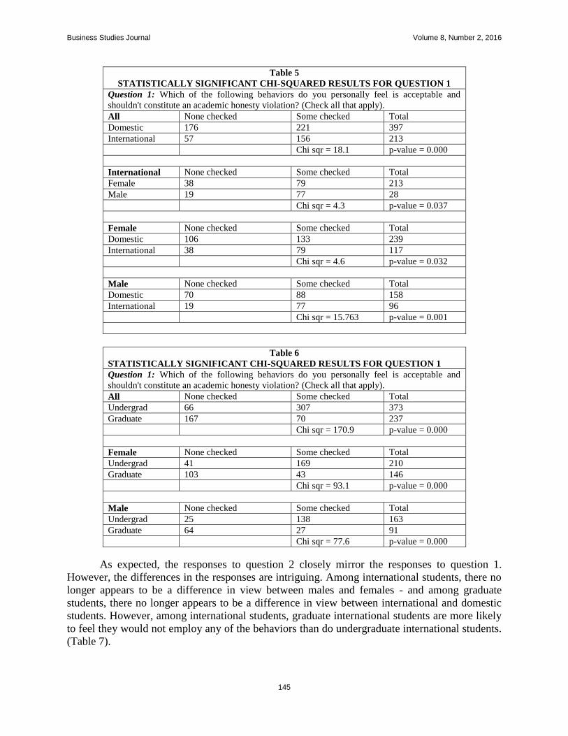
Business Studies Journal Volume 8, Number 2, 2016
145
Table 5
STATISTICALLY SIGNIFICANT CHI-SQUARED RESULTS FOR QUESTION 1
Question 1: Which of the following behaviors do you personally feel is acceptable and
shouldn't constitute an academic honesty violation? (Check all that apply).
All None checked Some checked Total
Domestic 176 221 397
International 57 156 213
Chi sqr = 18.1 p-value = 0.000
International None checked Some checked Total
Female 38 79 213
Male 19 77 28
Chi sqr = 4.3 p-value = 0.037
Female None checked Some checked Total
Domestic 106 133 239
International 38 79 117
Chi sqr = 4.6 p-value = 0.032
Male None checked Some checked Total
Domestic 70 88 158
International 19 77 96
Chi sqr = 15.763 p-value = 0.001
Table 6
STATISTICALLY SIGNIFICANT CHI-SQUARED RESULTS FOR QUESTION 1
Question 1: Which of the following behaviors do you personally feel is acceptable and
shouldn't constitute an academic honesty violation? (Check all that apply).
All None checked Some checked Total
Undergrad 66 307 373
Graduate 167 70 237
Chi sqr = 170.9 p-value = 0.000
Female None checked Some checked Total
Undergrad 41 169 210
Graduate 103 43 146
Chi sqr = 93.1 p-value = 0.000
Male None checked Some checked Total
Undergrad 25 138 163
Graduate 64 27 91
Chi sqr = 77.6 p-value = 0.000
As expected, the responses to question 2 closely mirror the responses to question 1.
However, the differences in the responses are intriguing. Among international students, there no
longer appears to be a difference in view between males and females - and among graduate
students, there no longer appears to be a difference in view between international and domestic
students. However, among international students, graduate international students are more likely
to feel they would not employ any of the behaviors than do undergraduate international students.
(Table 7).

Business Studies Journal Volume 8, Number 2, 2016
146
Table 7
STATISTICALLY SIGNIFICANT CHI-SQUARED RESULTS FOR QUESTION 2
Question 2: Which of the following behaviors do you feel you might do if you felt there
would be no legal or academic repercussions from it? (Check all that apply).
International None checked Some checked Total
Undergrad 0 192 192
Graduate 9 19 28
Chi sqr = 64.3 p-value = 0.000
CONCLUSION AND RECOMMENDATIONS FOR FUTURE RESEARCH
“American educators should understand that it is very likely that their non-American
students (at home or abroad) have a different perception of what is or is not cheating. Further, the
non-American students and a U.S. educator may also have very different perspectives concerning
the role instructors should play in the prevention of cheating.” (Lupton, Chapman, Weiss, 2000,
p. 235). We continue on the early direction of research which was primarily US-based and
studying characteristics, attributes and situations of the students. We add to the current research
which is looking at students across cultures and across education levels. Since 2000 there have
been several studies that document the differences between students at one international site or
country, but the topic has not been fully explored. Our results quantitatively validate the
perceived difference in international students that has been observed by instructors as they teach
in different countries.
We also looked at the self-reported opinions of students towards academic dishonesty and
found less difference in domestic male and female students but statistically significant
differences between international students and domestic students and between graduate and
undergraduate students. Also, similar to Iyer and Eastman (2006), we found some evidence to
suggest gender differences do exist, but lessen as students proceed to graduate status.
The scope of this survey is narrow. It could improve with additional questions. It would be
interesting to expand the survey questions to query “why,” in order to identify student reasoning.
In the future, we would like to expand our survey to include other forms of academic dishonesty.
Just as many current studies are reporting, we found that there are differences in the
perceptions and tolerance of students from different countries. International students appear more
tolerant of academic dishonesty than their domestic counterparts. The gender-based analysis of
the responses produced no surprises. There are more gender-related differences among the
international students and fewer differences among domestic graduate students.
REFERENCES
Bailey, W. C. & S. Scott Bailey (2011). A Comparison of Attitudes Towards Cheating Between Domestic &
International Students. International Journal of Business Research, 11(3), 26-37.
Bailey, W. C. & S. Scott Bailey (2011). Do Online and Lecture Students View Cheating Differently? Review of
Business Research, 11(3), 37-47.
Bailey, W. C., S. Scott Bailey & Connie Nott (2014). International Students Do View Cheating Differently.
International Journal of Business Research, 14(1) 134-143.
Chapman, Kenneth J. & Robert A. Lupton (2004). Academic Dishonesty in a Global educational market: a
comparison of Hong Kong and American university business students. The International Journal of
Educational Management, 18(6/7), 425-435.
Iyer, Rajesh & Jacqueline Eastman (2006). "Academic Dishonesty: Are Business Students Different From Other
College Students?” Journal of Education for Business, 82(2), 101-110.

Business Studies Journal Volume 8, Number 2, 2016
147
Jurdi, R., H.S. Hage, & H.P.H. Chow (2011). Academic dishonesty in the Canadian classroom: Behaviours of a
sample of university students. The Canadian Journal of Higher Education, 41(3), 1-35. Retrieved January
10th
, 2014 from http://search.proquest.com/docview/921581103?accountid=38769
Lin, C. S., & L.M. Wen (2007). Academic dishonesty in higher education--a nationwide study in Taiwan. Higher
Education, 54(1), 85-97. Retrieved January 10th
, 2014 from doi:http://dx.doi.org/10.1007/s10734-006-
9047-z. 2007.
Lupton, Robert A., Kenneth J. Chapman & John E. Weiss (2000). A Cross-National Exploration of Business
Students’ Attitudes, Perceptions, and Tendencies towards Cheating, Journal of Education for Business,
75(4), 231 - 235.
Rakovski, Carter C. & Elliott S. Levy (2007). Academic Dishonesty: Perceptions of Business Students. College
Student Journal, 41(2), 466-481.
Smyth, Lynnette S., James R. Davis & Charles O. Knoncke (2009). Students' Perceptions of Business Ethics: Using
Cheating as a Surrogate for Business Situations. Journal of Education for Business, 84(4), 229-239.