BV0056-11 TR Cover2004.qxd 23-03-2004 13:33 Page 1 ...Vibration Measurement A/S, DK-2850 Nærum, Denmark. Editor: Harry K. Zaveri bv005611.book Page iii Tuesday, March 23, 2004 12:46

TECHNICAL REVIEW

Beamforming

HEADQUARTERS: DK-2850 Nærum · DenmarkTelephone: +45 4580 0500 · Fax: +45 4580 14 05www.bksv.com · [email protected]

BV

0056

–11

ISSN

000

7–26

21

No.1 2004

BV0056-11_TR_Cover2004.qxd 23-03-2004 13:33 Page 1

Previously issued numbers ofBrüel & Kjær Technical Review1 – 2002 A New Design Principle for Triaxial Piezoelectric Accelerometers

Use of FE Models in the Optimisation of Accelerometer DesignsSystem for Measurement of Microphone Distortion and Linearity from Medium to Very High Levels

1 – 2001 The Influence of Environmental Conditions on the Pressure Sensitivity of Measurement MicrophonesReduction of Heat Conduction Error in Microphone Pressure Reciprocity CalibrationFrequency Response for Measurement Microphones – a Question of ConfidenceMeasurement of Microphone Random-incidence and Pressure-field Responses and Determination of their Uncertainties

1 – 2000 Non-stationary STSF1 – 1999 Characteristics of the Vold-Kalman Order Tracking Filter1 – 1998 Danish Primary Laboratory of Acoustics (DPLA) as Part of the National

Metrology OrganisationPressure Reciprocity Calibration – Instrumentation, Results and UncertaintyMP.EXE, a Calculation Program for Pressure Reciprocity Calibration of Microphones

1 – 1997 A New Design Principle for Triaxial Piezoelectric AccelerometersA Simple QC Test for Knock SensorsTorsional Operational Deflection Shapes (TODS) Measurements

2 – 1996 Non-stationary Signal Analysis using Wavelet Transform, Short-time Fourier Transform and Wigner-Ville Distribution

1 – 1996 Calibration Uncertainties & Distortion of Microphones.Wide Band Intensity Probe. Accelerometer Mounted Resonance Test

2 – 1995 Order Tracking Analysis1 – 1995 Use of Spatial Transformation of Sound Fields (STSF) Techniques in the

Automative Industry2 – 1994 The use of Impulse Response Function for Modal Parameter Estimation

Complex Modulus and Damping Measurements using Resonant and Non-resonant Methods (Damping Part II)

1 – 1994 Digital Filter Techniques vs. FFT Techniques for Damping Measurements (Damping Part I)

2 – 1990 Optical Filters and their Use with the Type 1302 & Type 1306 Photoacoustic Gas Monitors

1 – 1990 The Brüel & Kjær Photoacoustic Transducer System and its Physical Properties

2 – 1989 STSF — Practical Instrumentation and ApplicationDigital Filter Analysis: Real-time and Non Real-time Performance

1 – 1989 STSF — A Unique Technique for Scan Based Near-Field Acoustic Holography Without Restrictions on Coherence

(Continued on cover page 3)

bv005611.book Page i Tuesday, March 23, 2004 12:46 PM

TechnicalReviewNo. 1 – 2004

bv005611.book Page ii Tuesday, March 23, 2004 12:46 PM

Contents

Beamforming .......................................................................................................... 1J.J. Christensen and J. Hald

Copyright © 2004, Brüel & Kjær Sound & Vibration Measurement A/SAll rights reserved. No part of this publication may be reproduced or distributed in any form, or by any means, without prior written permission of the publishers. For details, contact: Brüel & Kjær Sound & Vibration Measurement A/S, DK-2850 Nærum, Denmark.

Editor: Harry K. Zaveri

bv005611.book Page iii Tuesday, March 23, 2004 12:46 PM

1

Beamforming

by J.J. Christensen and J. Hald

AbstractThis article explains the basic principles of Beamforming, including the main per-formance parameters Resolution and Sidelobe Level. Special attention is given tothe influence of array design and to cross-spectral beamforming. Different arraydesigns, including Brüel & Kjær’s newly patented wheel array design, are describedand compared, and the basic principle of Brüel & Kjær’s geometry optimisationmethod is outlined. A new, improved version of cross-spectral beamforming usedin Beamforming Software Type 7768 is introduced and its benefits are verified. Thearticle also provides some guidelines for performing good measurements andfinally, describes a set of measurements representing typical applications.

RésuméCet article traite succintement du concept d’imagerie par formation de faisceaux, etnotamment des principaux paramètres essentiels aux performances de l’antenneque sont la Résolution et le Niveau de lobe latéral. Une attention toute particulièreest portée sur l’influence de la forme de l’antenne et sur la formation de faisceauxpar approche interspectrale. Diverses conceptions d’antennes, dont l’antenne circu-laire Brüel & Kjær nouvellement brevetée, y sont présentées et comparées; les prin-cipes fondamentaux de la méthode propriétaire d’optimisation géométrique y sontsoulignés. Une nouvelle version amendée de l’approche interspectrale implémen-tée dans le Logiciel Beamforming Software Type 7768 est également présentée etses avantages sont vérifiés. Cet article inventorie par ailleurs les points contribuantà la réalisation de mesures de qualité, pour conclure par la description d’une sériede mesures se rapportant à des applications typiques.

ZusammenfassungDieser Artikel erläutert die Grundprinzipien des Beamforming einschließlich derHauptparameter Auflösung und Nebenmaxima (Sidelobe Level). Besondere Auf-merksamkeit wird dem Einfluss der Array-Konstruktion und dem Beamformingnach dem Kreuzspektrum-Verfahren gewidmet. Es werden verschiedene Array-

bv005611.book Page 1 Tuesday, March 23, 2004 12:46 PM

2

Konstruktionen beschrieben und verglichen, darunter Brüel & Kjærs patentiertesWheel Array. Außerdem wird das Grundprinzip der Geometrieoptimierung vonBrüel & Kjær skizziert. Eine neue verbesserte Version des in der BeamformingSoftware Typ 7768 verwendeten Beamforming nach dem Kreuzspektrum-Verfah-ren wird vorgestellt und dessen Vorteile nachgewiesen. Der Artikel enthält auchRichtlinien zur Durchführung guter Messungen und beschreibt eine Serie von Mes-sungen, die typische Anwendungen repräsentieren.

IntroductionPlanar Near-field Acoustical Holography (NAH) is an established technique forefficient and accurate noise source location [1, 2]. NAH can provide high-resolu-tion source maps on a planar source surface from measurements taken over a regu-lar rectangular grid of points close to the source. The measurement grid mustcapture the major part of the sound radiation into a half space and therefore com-pletely cover the noise source plus approximately a 45º solid angle. The grid spac-ing must be less than half a wavelength at the highest frequency of interest. Thus,the number of measurement points gets very high when the source is much largerthan the wavelength, which always occurs at sufficiently high frequencies. Thesame problem arises when for some reason it is not possible to measure close tothe source. Then, because of the required 45º coverage angle, the measurementarea must be very large. In these cases, beamforming is an attractive alternative.

Beamforming is an array-based measurement technique for sound-source loca-tion from medium to long measurement distances. Basically, the source location isperformed by estimating the amplitudes of plane (or spherical) waves incidenttowards the array from a chosen set of directions. The angular resolution isinversely proportional to the array diameter measured in units of wavelength, sothe array should be much larger than wavelength to get a fine angular resolution. Atlow frequencies, this requirement usually cannot be met, so here the resolution willbe poor. Unlike NAH, beamforming does not require the array to be larger than thesound source. For typical, irregular array designs, the beamforming method doesnot allow the measurement distance to be much smaller than the array diameter. Onthe other hand, the measurement distance should be kept as small as possible toachieve the finest possible resolution on the source surface.

An important difference between beamforming and NAH is that beamformingcan use irregular array geometries, for example, random array geometries. The useof a discrete set of measurement points on a plane can be seen as a spatial sampling


3

of the sound field. NAH requires a regular, rectangular grid of points in order toapply a 2D spatial DFT. Outside the near-field region, such a regular grid will sup-press spatial aliasing effects very well, if the grid spacing is just less than half awavelength. When the grid spacing exceeds half a wavelength, spatial aliasingcomponents quickly get very disturbing. Irregular arrays on the other hand canpotentially provide a much smoother transition: spatial aliasing effects can be keptat an acceptable level up to a much higher frequency with the same average spatialsampling density. This indicates why beamforming can measure up to high fre-quencies with a fairly low number of microphones.

Theory

Delay-And-Sum Beamforming for Infinite Focus DistanceThe principle of Beamforming is best introduced through a description of the basicDelay-and-Sum beamformer. As illustrated in Fig. 1, we consider a planar array ofM microphones at locations rm (m = 1, 2, …, M) in the xy-plane of our coordinatesystem. When such an array is applied for Delay-and-Sum Beamforming, themeasured pressure signals pm are individually delayed and then summed [3]:

Fig. 1. (a) A microphone array, a far-field focus direction, and a plane wave incident from thefocus direction. (b) A typical directional sensitivity diagram with a main lobe in the focus direc-tion and lower sidelobes in other directions

Plane wave

– �

�

(a) 040009(b)

–90º

– 60º

– 30º0º

30º

60º

90º

10 dB

20 dB

30 dBSidelobe Main lobe


4

(1)

where wm are a set of weighting or shading coefficients applied to the individualmicrophone signals. The individual time delays ∆m are chosen with the aim ofachieving selective directional sensitivity in a specific direction, characterisedhere by a unit vector �. This objective is met by adjusting the time delays in such away that signals associated with a plane wave, incident from the direction �, willbe aligned in time before they are summed. Geometrical considerations (Fig. 1)show that this can be obtained by choosing:

(2)

where c is the propagation speed of sound. Signals arriving from other far-fielddirections will not be aligned before the summation, and therefore they will notadd up coherently. Thus, we have obtained a directional sensitivity, as illustratedin Fig. 1(b).

The frequency domain version of eq. (1) for the Delay-and-Sum beamformeroutput is:

(3)

Here, x is the temporal angular frequency, k ≡ –k� is the wave number vector of aplane wave incident from the direction � in which the array is focused (see Fig. 1),and k = x/c is the wave number. In eq. (3) an implicit time factor equal to e jxt isassumed. Because k ≡ –k�, we can write B(k, x) instead of B(�, x).

Through our choice of time delays ∆m(�), or equivalently of the “preferred”wave number vector k ≡ –k�, we have “tuned” the beamformer on the far-fielddirection �. Ideally, we would like to measure only signals arriving from that direc-tion, in order to get a perfect localisation of the sound sources. To investigate, howmuch “leakage” we will get from plane waves incident from other directions, wenow assume a plane wave incident with a wave number vector k0 different from thepreferred k ≡ –k�, Fig. 2. The pressure measured by the microphones will then be:

(4)

which, according to eq. (3), will give the following output from the beamformer:

b � t,( ) wmm 1=

M

∑ pm t ∆m �( )–( )=

∆m

� rm⋅c

--------------=

B � x,( ) wmPm x( )ejx∆m �( )–

m 1=

M

∑ wmPm x( )ejk rm⋅

m 1=

M

∑= =

Pm x( ) P0ejk0 rm⋅–

=


5

(5)

Here, the function W,

(6)

is the so-called Array Pattern. It has the form of a generalised spatial DFT of theweighting function w, which equals zero outside the array area. In the case of uni-form shading, wm ≡ 1, the array pattern, eq. (6), depends only on the array geome-try. In the following we shall mainly be concerned with uniform shading and will

Fig. 2. A plane wave, with wave number vector k0, incident from a direction different from thefocus direction �. For a planar array the beamformer output, eq. (5), is a function of the differ-ence K of the projections and of the wave number vectors k0 and k onto the planedefined by the array

k0 k

≡ – �

�

–

040010^ ^

^

B � x,( ) P0 wmej k k0–( ) rm⋅

P0W k k0–( )≡m 1=

M

∑=

W K( ) wmejK rm⋅

m 1=

M

∑≡


6

consequently omit the wm term from the equations. The effect of non-uniformshading is discussed in “Regular Arrays” on page 19.

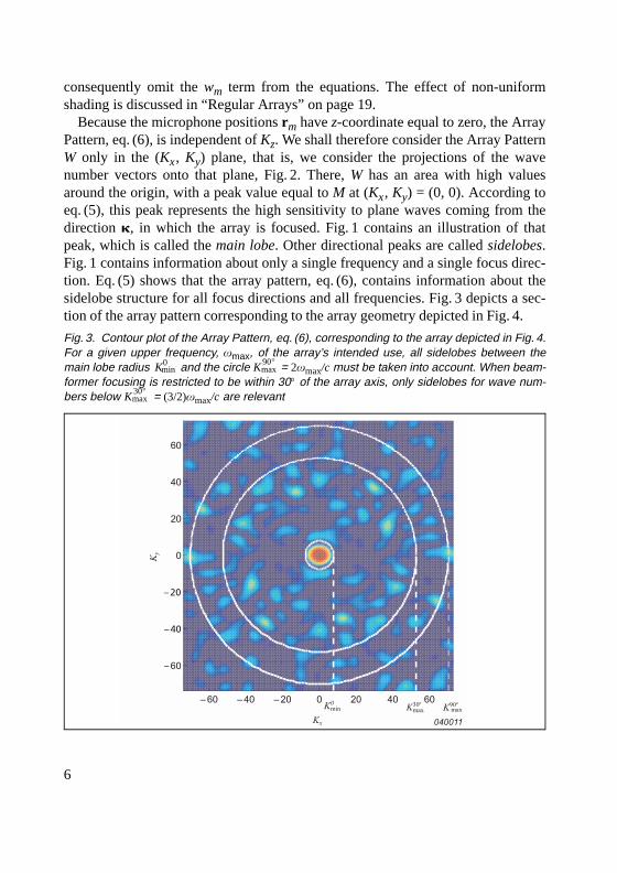
Because the microphone positions rm have z-coordinate equal to zero, the ArrayPattern, eq. (6), is independent of Kz. We shall therefore consider the Array PatternW only in the (Kx, Ky) plane, that is, we consider the projections of the wavenumber vectors onto that plane, Fig. 2. There, W has an area with high valuesaround the origin, with a peak value equal to M at (Kx, Ky) = (0, 0). According toeq. (5), this peak represents the high sensitivity to plane waves coming from thedirection �, in which the array is focused. Fig. 1 contains an illustration of thatpeak, which is called the main lobe. Other directional peaks are called sidelobes.Fig. 1 contains information about only a single frequency and a single focus direc-tion. Eq. (5) shows that the array pattern, eq. (6), contains information about thesidelobe structure for all focus directions and all frequencies. Fig. 3 depicts a sec-tion of the array pattern corresponding to the array geometry depicted in Fig. 4.

Fig. 3. Contour plot of the Array Pattern, eq. (6), corresponding to the array depicted in Fig. 4.For a given upper frequency, xmax, of the array’s intended use, all sidelobes between themain lobe radius and the circle = 2xmax/c must be taken into account. When beam-former focusing is restricted to be within 30° of the array axis, only sidelobes for wave num-bers below = (3/2)xmax/c are relevant

K0min K

90°max

K30°max

–

– 40

– 20


7

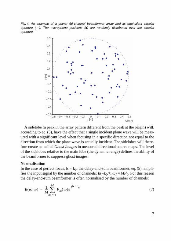
A sidelobe (a peak in the array pattern different from the peak at the origin) will,according to eq. (5), have the effect that a single incident plane wave will be meas-ured with a significant level when focusing in a specific direction not equal to thedirection from which the plane wave is actually incident. The sidelobes will there-fore create so-called Ghost Images in measured directional source maps. The levelof the sidelobes relative to the main lobe (the dynamic range) defines the ability ofthe beamformer to suppress ghost images.

NormalisationIn the case of perfect focus, k = k0, the delay-and-sum beamformer, eq. (5), ampli-fies the input signal by the number of channels: B(–k0/k, x) = MP0. For this reasonthe delay-and-sum beamformer is often normalised by the number of channels:

(7)

Fig. 4. An example of a planar 66-channel beamformer array and its equivalent circularaperture (---). The microphone positions (● ) are randomly distributed over the circularaperture

B � x,( ) 1M----- Pm x( )e

jk rm⋅

m 1=

M

∑=


8

ResolutionThe resolution of a beamformer describes its ability to distinguish waves incidentfrom directions close to each other. When focusing on sources in the far field, res-olution is the smallest angular separation between two plane waves that allowsthem to be separated, and for sources at a finite distance a practical definition ofresolution is the minimum distance between two sources such that they can be sep-arated.

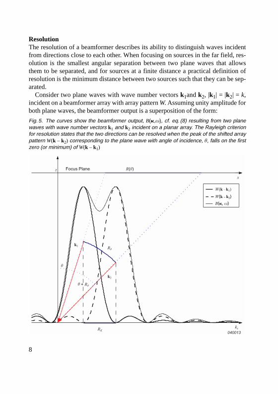
Consider two plane waves with wave number vectors k1and k2, |k1| = |k2| = k,incident on a beamformer array with array pattern W. Assuming unity amplitude forboth plane waves, the beamformer output is a superposition of the form:

Fig. 5. The curves show the beamformer output, B(�,x), cf. eq. (8) resulting from two planewaves with wave number vectors k1 and k2 incident on a planar array. The Rayleigh criterionfor resolution states that the two directions can be resolved when the peak of the shifted arraypattern W(k – k2) corresponding to the plane wave with angle of incidence, h, falls on the firstzero (or minimum) of W(k – k1)

( – )

(�, x)

h

h h

h

h


9

B(�, x) = W(k – k1) + W(k – k2) (8)

cf. eq. (5). The Rayleigh criterion [3] states that the two directions can be justexactly resolved when the peak of W(k – k2) falls on the first zero of W(k – k1), cf.Fig. 5. Assuming that the required angular separation between k1and k2 is small, itcan be shown (see “Appendix: Resolution” on page 47) that at finite distance, z,the minimum resolvable source separation in the radial direction, R(h), is givenby:

(9)

where RK is the main lobe width in the array pattern and h is the off-axis angle.The value of RK is, according to the Rayleigh criterion, given by the first null(minimum), K0

min, of the array pattern: RK = K0min. The exact value depends on the

positions of all the array microphones through eq. (6), but a good general estimatecan be calculated by considering the limiting cases where we have an infinitenumber of transducers uniformly distributed over a line segment of length D or acircular disc with radius D/2. In other words, we imagine we are able to sample thesound field at all points within an area (aperture) instead of only at a few discretepositions. In this continuous case we should use an integral expression for thearray pattern, eq. (6), the aperture smoothing function:

(10)

where d = 1 for the line segment, d = 2 for the circular aperture and w(r) is now acontinuous shading function. In the case of uniform shading, eq. (10) can be evalu-ated to, J1 being the Bessel function of order 1 [3]:

(11)

(12)

From eq. (11) and eq. (12) we find that the first zero in the array pattern corre-sponding to the line segment and the circular aperture occurs at:

(13)

R h( )zRK

k--------- 1

cos3h

-------------=

W K( ) 1

2p( )d-------------- w r( )e

jK r⋅d

dr

r D 2⁄<∫=

W Kx( )KxD 2⁄( )sin

Kx 2⁄------------------------------ ,= d 1=

W K( ) pDK

--------J1 KD 2⁄( ),= K Kx2

Ky2

+ ,= d 2=

Kmin0

a2pD------=


10

where a =1 for the linear aperture and a ≈ 1.22 for the circular aperture. Now,using the fact that the wave number k is related to the wavelength, k, by k = 2p/kwe obtain by insertion into eq. (9) the desired expression for beamformer resolu-tion:

(14)

For on-axis incidence, h = 0, the resolution is given by:

(15)

We notice that the resolution is proportional to the wavelength and becomes bet-ter with larger aperture size, but worse with increasing array to object distance.This relation is not limited to acoustics; the reader may be familiar with the fact thatthe ability of an optical camera to resolve details depends on the lens diameter andthe distance to the object.

Comparing the on-axis and general off-axis resolution, eq. (15) and eq. (14), wenotice that the ratio between them is given by:

(16)

This ratio is depicted in Fig. 6 and we observe that for angles of incidence morethan 30° off-axis, the resolution becomes more than 50% greater than the on-axisresolution. For this reason the useful beamformer opening angle is in practicerestricted to 30°.Fig. 6. The variation of the ratio between off-axis and on-axis resolution as given by eq. (16)

R h( ) a

cos3h

------------- zD----k=

RAxis a zD----

k=

R h( )RAxis-------------- 1

cos3h

-------------=

h

h


11

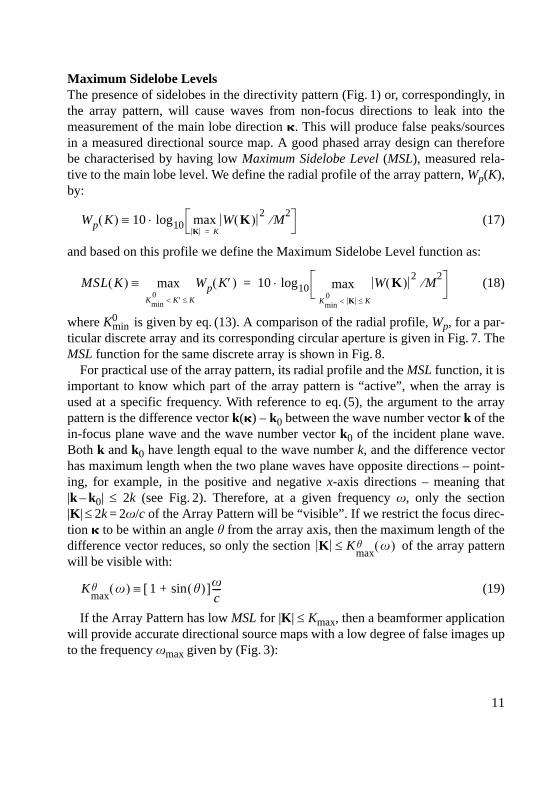
Maximum Sidelobe LevelsThe presence of sidelobes in the directivity pattern (Fig. 1) or, correspondingly, inthe array pattern, will cause waves from non-focus directions to leak into themeasurement of the main lobe direction �. This will produce false peaks/sourcesin a measured directional source map. A good phased array design can thereforebe characterised by having low Maximum Sidelobe Level (MSL), measured rela-tive to the main lobe level. We define the radial profile of the array pattern, Wp(K),by:

(17)

and based on this profile we define the Maximum Sidelobe Level function as:

(18)

where K0min is given by eq. (13). A comparison of the radial profile, Wp, for a par-

ticular discrete array and its corresponding circular aperture is given in Fig. 7. TheMSL function for the same discrete array is shown in Fig. 8.

For practical use of the array pattern, its radial profile and the MSL function, it isimportant to know which part of the array pattern is “active”, when the array isused at a specific frequency. With reference to eq. (5), the argument to the arraypattern is the difference vector k(�) – k0 between the wave number vector k of thein-focus plane wave and the wave number vector k0 of the incident plane wave.Both k and k0 have length equal to the wave number k, and the difference vectorhas maximum length when the two plane waves have opposite directions – point-ing, for example, in the positive and negative x-axis directions – meaning that|k – k0| ≤ 2k (see Fig. 2). Therefore, at a given frequency x, only the section|K| ≤ 2k = 2x/c of the Array Pattern will be “visible”. If we restrict the focus direc-tion � to be within an angle h from the array axis, then the maximum length of thedifference vector reduces, so only the section of the array patternwill be visible with:

(19)

If the Array Pattern has low MSL for |K| ≤ Kmax, then a beamformer applicationwill provide accurate directional source maps with a low degree of false images upto the frequency xmax given by (Fig. 3):

Wp K( ) 10 log10 maxK K=

W K( ) 2M

2⁄⋅≡

MSL K( ) maxKmin

0K ′ K≤<

Wp K′( )≡ 10 log10 maxKmin

0K< K≤

W K( ) 2M

2⁄⋅=

K Khmax

x( )≤

Khmax

x( ) 1 h( )sin+[ ]xc----≡


12

(20)

As an example, if the beamformer will be focused on directions � not more than30° off-axis, then the upper limiting frequency becomes xmax(30º) = 2/3Kmaxc(Fig. 3). We notice the general relation:

(21)

Fig. 7. Comparison of the aperture smoothing function, eq. (12), for a circular aperture andthe radial array pattern profile of eq. (18) for a “circular” 66-channel discrete array with thesame diameter (Fig. 4). The aperture smoothing function of the uniformly shaded circularaperture represents the, theoretically, best sidelobe suppression attainable. Due to the finitenumber of points sampled with the discrete array, the sidelobe levels are much higher. Themain lobe widths of the discrete array and the equivalent circular aperture are nearly identicalas this quantity is determined by the aperture size

Khmax

xmax( ) Kmax xmax h( )Kmaxc

1 h( )sin+-------------------------=⇒=

xmax 30°( ) 43---xmax 90°( )=


13

Eq. (19) is a linear relation between frequency x and the highest array patternwave number that is active at that frequency. The argument K ofthe MSL function, eq. (18), is exactly an upper limiting wave number in the arraypattern, so therefore it is straightforward to use as argument in theMSL function. Thereby we have expressed the MSL as a function of frequency x:

. In order to calculate the MSL at a given frequency, one needs tospecify the maximum focusing angle h. We have chosen to always show or specifythe worst case , that is, no restriction on focus direction.

Cross-spectral Formulation with Exclusion of AutospectraFor stationary sound fields it is natural to operate with averaged cross- and auto-spectra, and it turns out that exclusion of autospectra in beamforming calculations

Fig. 8. The sidelobe level profile, Wp, eq. (17) and the maximum sidelobe level functionMSL(K), eq. (18), for the array depicted in Fig. 4. The functions are extracted from the corre-sponding array pattern of Fig. 3

K Khmax x( )=

K Khmax x( )=

MSL[K hmax x( )]

MSL[K 90°max x( )]


14

is advantageous in several respects. The average power output from the Delay-and-Sum beamformer can be derived from eq. (3):

(* indicates complex conjugate) (22)

where we have introduced the cross-spectrum matrix:

We may split eq. (22) into an autospectrum part and a cross-spectrum part:

(23)

Here, the autospectra Cmm will contain self-noise from the individual channels,such as wind-noise and electronic noise from the data acquisition hardware. Forthat reason it would be desirable to omit the first sum in eq. (23). Ideally, the cross-spectra Cnm, m ≠ n, are not affected by the self-noise, because the self-noise in onechannel is generally incoherent with the self-noise in any other channel. Underthat condition, averaging will suppress contributions from self-noise in the cross-spectra. We can assess the effect of excluding the autospectra by considering theplane wave response of the cross-spectral beamformer. For a plane wave withwave number vector k0 and amplitude P0 the pressure recorded by the mth micro-phone is Pm = P0exp(–jk0rm). Insertion of this in eq. (22) leads to the followingexpression for the beamformer power output:

(24)

where we have introduced the Power Array Pattern:

V � x,( ) B � x,( ) 2≡ Pm x( )Pn* x( )ejk rm rn–( )⋅

m n, 1=

M

∑=

Cnm x( )m n, 1=

M

∑ ejk rm rn–( )⋅

=

Cnm x( ) Pm x( )Pn* x( )≡

V � x,( ) Cmmm 1=

M

∑ Cnmejk rm rn–( )⋅

m n≠

M

∑+=

V � x,( ) P02

ej– k0 rm rn–( )⋅

ejk rm rn–( )⋅

m n, 1=

M

∑=

P02

ej k k0–( ) rm rn–( )⋅

m n, 1=

M

∑= = P02U k k0–( )


15

(25)

In a similar way we see that the self-term-free versions of the power array pat-tern, eq. (25), and the cross-spectral beamformer response, eq. (23):

(26)

are for plane waves related by:

V ′(�, x) = |P0|2U ′(k – k0) (27)

Thus, removal of the autospectral terms from the cross-spectral beamformer,eq. (23), corresponds to omitting the self-terms from the definition of the powerarray pattern, eq. (25). Provided the reduced array pattern U ′ has lower sidelobelevel than U, we can therefore reduce the level of ghost images in cross-spectralbeamformer output by omitting the autospectra.

Comparing the definitions of the array pattern U and the reduced version U ′ wefind that:

U ′(K) = U(K) – M (28)

The main lobe is therefore reduced from M2 (for U) to M2 – M (for U ′), and thehighest sidelobe is reduced from M2·10MSL/10 to M2·10MSL/10 – M. Assuming firstthat U ′ does not become negative, this leads to the following Maximum SidelobeLevel for U ′:

which is easily shown to be always smaller (better) than MSL. As an example, forthe 66-channel array depicted in Fig. 4, the MSL equals –9.5 dB over a wide fre-quency range. Over that frequency range MSL ′ equals –10.1 dB, meaning that thehighest sidelobe has been reduced by 0.6 dB (Fig. 8). At lower frequencies the gainis bigger. If the power array pattern U contains values less than M, then thereduced array pattern U ′ will have areas with negative values. The worst case iswhen U has a null. In that case the minimum value of U ′ equals –M, which willhave the same effect as a sidelobe with amplitude equal to M. Such a sidelobe willnot affect MSL ′ as long as M is smaller than M2·10MSL/10 – M. This condition has

U K( ) W K( ) 2≡ ejK rm rn–( )⋅

m n, 1=

M

∑=

U′ K( ) ejK rm rn–( )⋅

m n≠

M

∑≡ and V′ � x,( ) Cnmejk rm rn–( )⋅

m n≠

M

∑≡

MSL′ 10 log10M

210⋅

MSL 10⁄M–

M2

M–-----------------------------------------------

⋅ 10 log10M 10

MSL 10⁄⋅ 1–M 1–

------------------------------------------ ⋅= =


16

been fulfilled for all the arrays that we have been designing. Additionally, thisworst-case condition will not occur, when only array geometries without redun-dant spacing vectors are used.

Finite Focus DistanceUp to now we have only considered the resolution of incoming plane waves, cor-responding to point sources at infinite distance. The time delays ∆m of eq. (2) werechosen with the aim of aligning in time the signals of a plane wave arriving fromthe far-field direction � before the summation of the Delay-And-Sum beamform-ing, eq. (1). Use of a plane wave for calculation of the delays corresponds to focus-ing of the array at infinite distance in the chosen direction. To focus on a pointsource at a finite distance, the delays should align in time the signals of a sphericalwave radiated from the focus point.

The expression for Delay-And-Sum beamforming for focusing at a point r at afinite distance becomes:

(29)

Here we have replaced the delays, eq. (2), with the form:

(30)

where rm(r) ≡ |r – rm| is the distance from microphone m to the focus point, Fig. 9.The near-field version of eq. (23) for the beamformer power output appears as:

(31)

Cross-spectral Imaging FunctionEq. (31) for finite-distance beamforming contains no compensation for the factthat different positions on the assumed source plane have different distances to thearray transducers and therefore are attenuated by different amounts. For a singlesource at ri, a possible correction could be to replace the cross-spectrum matrix bythe scaled version Cnmrm(ri)rn(ri). The introduction of a scaled cross-spectrummatrix is, however, an ad-hoc correction with uncontrolled effects. A soundapproach can be achieved by assuming a model where the recorded sound field isgenerated by a monopole distribution. For each position on the source plane the

B r x,( ) Pm x( )ej– x∆m r( )

m 1=

M

∑=

∆m r( )r rm r( )–

c-------------------------=

V r x,( ) Cmmm 1=

M

∑ Cnmejx ∆n r( ) ∆m r( )–[ ]

m n≠

M

∑+=


17

estimated source strength reflects how well the sound field from a monopole pointsource at that position fits the sound field measured by the array.

Let rm, m = 1, …, M, be the transducer coordinates and let r be the position of amonopole. The pressure, Pm, recorded by the mth transducer is then given byPm(r) ≡ P0vm(r) = P0v(rm – r), where P0 is the source strength and v(r) is the steer-ing vector given by:

v(r) = e–jk|r |/|r | (32)

and the cross-spectrum, , between channel m and n is:

(33)

where a is a real amplitude coefficient. Then we define an error function, E(a, r),between the model cross-spectra and the measured cross-spectra, Cnm:

(34)

As shown in “Appendix: The Cross-spectral Imaging Function” on page 43, theminimisation of this error function corresponds to the maximisation of the Cross-spectral Imaging Function defined by:

Fig. 9. In near-field focusing, spherical waves emitted by a monopole source at the focuspoint r are assumed. Signal delays are computed according to eq. (30)

Cmodnm

Cmodnm P*

n Pm av*n

r( )vm r( )= =

E a r,( ) Cnm Cmodnm–

2Cnm av*

nr( )vm r( )–

2

m n, 1=

M

∑=m n, 1=

M

∑=


18

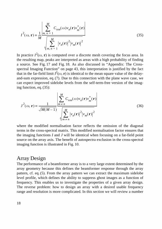
(35)

In practice I2(x, r) is computed over a discrete mesh covering the focus area. Inthe resulting map, peaks are interpreted as areas with a high probability of findinga source. See Fig. 17 and Fig. 18. As also discussed in “Appendix: The Cross-spectral Imaging Function” on page 43, this interpretation is justified by the factthat in the far-field limit I2(x, r) is identical to the mean square value of the delay-and-sum expression, eq. (7). Due to this connection with the plane wave case, wecan expect improved sidelobe levels from the self-term-free version of the imag-ing function, eq. (35):

(36)

where the modified normalisation factor reflects the omission of the diagonalterms in the cross-spectral matrix. This modified normalisation factor ensures thatthe imaging functions I and J will be identical when focusing on a far-field pointsource on the array axis. The benefit of autospectra exclusion in the cross-spectralimaging function is illustrated in Fig. 10.

Array DesignThe performance of a beamformer array is to a very large extent determined by thearray geometry because this defines the beamformer response through the arraypattern, cf. eq. (5). From the array pattern we can extract the maximum sidelobelevel profile, which defines the ability to suppress ghost images as a function offrequency. This enables us to investigate the properties of a given array design.The reverse problem: how to design an array with a desired usable frequencyrange and resolution is more complicated. In this section we will review a number

I2

x r,( ) 1M-----

Cnm x( )vn r( )v*m

r( )m n, 1=

M

∑

vn r( ) 2vm r( ) 2

m n, 1=

M

∑--------------------------------------------------------------------≡

J2

x r,( ) 1

M M 1–( )----------------------------

Cnm x( )vn r( )v*m

r( )m n≠

M

∑

vn r( ) 2vm r( ) 2

m n≠

M

∑--------------------------------------------------------------≡


19

of array designs including both previously published, regular and irregular arraydesigns and novel, numerically optimised array geometries, Fig. 11.

As we shall see below, the maximum sidelobe levels can be improved by shad-ing, i.e., application of a smooth spatial window function. This improvement is,however, obtained at the expense of decreased resolution ability.

Regular ArraysThe simplest example of a regular array is the uniform line array (ULA), which isa one-dimensional linear array with equidistant microphone spacing. Though weare mainly interested in planar arrays, this array is well suited to demonstrate anumber of important features of regular beamformer arrays. The microphone coor-

Fig. 10. Comparison of the output of three different beamforming algorithms for a configura-tion with two incoherent 3 kHz monopole sources of equal strength. The data were generatedusing the array shown in Fig. 4. In the legend I refers to the full cross-spectral imaging func-tion, eq. (35), J is the cross-spectral imaging function, eq. (36), which excludes the autospec-tra, and B is the delay-and-sum algorithm, eq. (29). All curves are normalised to 0 dB atmaximum


20

dinates, xm, of a ULA with microphone spacing d and M ≡ 2M½+1 microphonescan be written as:

xm = (m – M½)d, m = 0, …, M – 1 (37)

In the case of uniform shading, the corresponding array pattern [3] can be evaluatedto:

(38)

We notice that eq. (38) is a periodic function of K, the period equalling 2p/d. Inaddition to the main lobe at K = 0, the ULA array pattern exhibits repetitions of themain lobe, so-called grating lobes, at the positions K = p(2p/d), p = ±1, ±2, …,Fig. 12(a).

Fig. 11. Examples of regular and irregular array configurations. (a) 65-ch. cross-array, (b) 64-ch. grid array, (c) 66-ch. optimised random array, (d) 66-ch. Archimedean spiral array, (e) 66-ch. optimised wheel array, (f) 66-ch. optimised half-wheel array

y [m

]

(c)

(e)

040019�

0.2

0

−0.2

−0.2x [m]

0.20

y [m

]

(a)

0

−0.5−0.5

x [m]0 0.5

0.5(b)

y [m

]

−0.5 0 0.5x [m]

−0.4

−0.2

0

0.2

0.4

x [m]

y [m

]

−0.5 0 0.50

0.2

0.4

0.6

0.8

1(f)

−0.5 0 0.5−0.5

x [m]

0

0.5

y [m

]

−0.4 −0.2 0 0.2 0.4x [m]

−0.4

−0.2

0

0.2

0.4

y [m

]

(d)

W K( ) MKd 2⁄( )sinKd 2⁄( )sin

--------------------------------=


21

Fig. 12. Graph (a) illustrates the side-lobe structure of a regular array with grid spacing d. Inaddition to the main lobe at K = 0, grating lobes occur at Kx = ± 2pKN, KN = p/d, where p is apositive integer. Also shown is the wave number vector k0 at incidence angle 30°, and thefocus direction wave number vector k in the direction –30°. In any case |k| = |k0| = k and wechoose a frequency such that k = 2KN. The projection kx

0 of k0 onto the x-axis equals theNyquist wave number KN, and for this reason both the main lobe and the grating lobe at 2KNcontributes when beamforming is performed in the entire visible region (indicated by thegreen line) –KN < kx < 3KN, where kx is the projection of k on to the x-axis. In the resultingdirectional source map (b) a ghost source is seen at h = –30° in addition to the true source ath = 30°. The directional source map (c) illustrates the situation for on-axis incidence at thesame frequency

0– 2

–

(a)

040021

(b)

– 90º

– 60º

– 30º0º

30º

60º

90º10 dB

20 dB30 dB

(c)

– 90º

– 60º

– 30º0º

30º

60º

90º

10 dB

20 dB

30 dB

040022


22

Plots of the ULA array pattern are depicted in Fig. 13 for both uniform shadingand shading with a Hamming window. Comparing the two curves we see that theeffect of the windowing is to lower the sidelobe levels and broaden the main lobe,that is, the dynamic range of the beamformer is improved at the cost of resolution.

Spatial AliasingWhen sampling a time domain signal with a constant sampling rate fs = 1/Ts, thehighest frequency that can be unambiguously reconstructed is given by theNyquist frequency, fN = fs/2 = 1/(2Ts), or the corresponding angular frequency,xN = 2pfN = p/Ts with a period of TN = 2Ts [4]. Similarly, when spatially samplinga signal with a sampling interval equal to d, then the spatial Nyquist angular fre-quency (the Nyquist wave number) is KN = p/d with a period length equal to 2d.Plane waves with wavelength shorter than kmin = 2d therefore cannot be unambig-

Fig. 13. Plot of the array pattern for a uniform linear array with uniform shading and with aHamming window applied. The effect of the window is to lower the sidelobes at the expenseof widening the main lobe

(m – 1)


23

uously reconstructed from the spatial samples, implying that the highest frequencyfmax with sufficient sampling density is:

(39)

In general, time signals with frequencies f ± pfs, p = 1, 2, …, cannot be distin-guished when sampled with a sampling frequency fs = 2fN, and therefore they willall contribute when we estimate the content of, for example, the frequency f. Simi-larly, plane waves with angular frequencies K ± pKs, p = 1, 2, …, on the measure-ment plane cannot be distinguished when sampled with a spatial angular samplingfrequency Ks = 2KN, and consequently they will all contribute when we estimatethe content of any one of them in a spatially sampled sound field.

Typically, when aliasing occurs in the processing of a time domain signal, thenthere is a frequency component f > fN that is under-sampled and will contribute at asingle frequency f + pfs in the “visible frequency range”, – fN ≤ f + pfs ≤ fN, p beingan integer. The term “visible” means that only frequency components in that rangewill be estimated and used. Aliasing in beamforming happens in the same way, buthere the “visible wave number range” is controlled by the beamforming algorithmand will not be restricted in the same way to –KN ≤ K + pKs ≤ KN. As stated ineq. (19), the visible range will be up to –2k ≤ K + pKs ≤ 2k, and therefore there maybe several aliased components. The effect is that an angle h of plane wave inci-dence will contribute at several aliased angles ha. This is illustrated in Fig. 12(a)where we consider measurement with a regular array with grid spacing d at a tem-poral frequency equal to twice the maximum frequency, eq. (39), for the array. Thewave number vector k0 of a plane incident wave is therefore twice as long as theNyquist wave number: |k0| = k = 2KN, KN = p/d. We consider a plane wave incidentin the xz-plane at an angle 30° from the array axis, meaning that the projection of k0on the array plane has length equal to the Nyquist wave number: kx

0 = –KN.According to eq. (5), the output from the beamformer will be given byB(kx, x) = P0W(kx – kx

0) when we focus on a plane wave incident with wave numbervector k with x-component kx. When focusing is scanned over all possible incidentplane waves with wave number vectors k in the xz-plane, |k| = k, then kx will scanthe interval from –k = –2KN to k = 2KN, meaning that the argument Kx = kx – kx

0 tothe array pattern will scan the interval from –KN = p/d to 3KN = 3p/d. By inspectionof the array pattern in Fig. 12(a) we see that maximum output will be obtained bothat the main lobe (Kx = 0) for kx = kx

0 = – KN and at the first grating lobe (Kx = 2KN)for kx = –kx

0 = KN. In the resulting directional source map, Fig. 12(b), the planewave incident at h = +30° contributes also as an aliasing component at ha = –30°.

fmaxc

kmin---------- c

2d------= =


24

For on-axis incidence at the same frequency, the resulting directional source map iseven more confusing since in addition to the main lobe, two grating lobes of thearray pattern at Kx = ±2KN are included, Fig. 12(c).

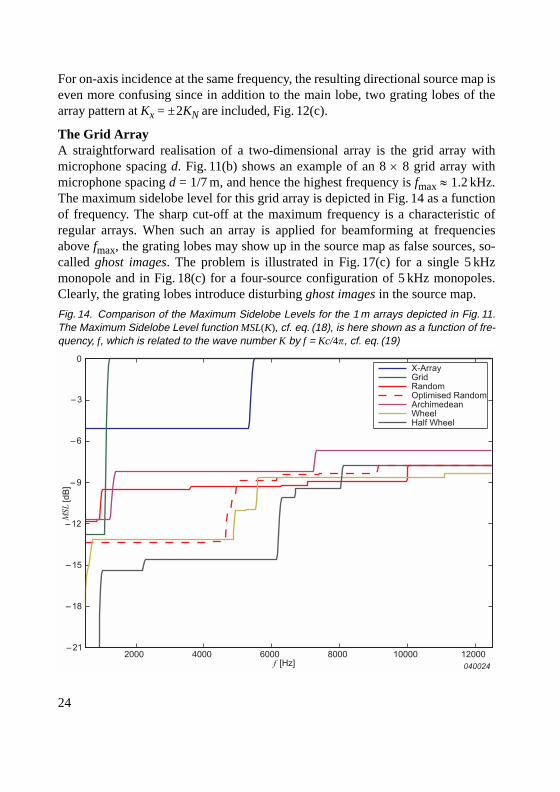
The Grid ArrayA straightforward realisation of a two-dimensional array is the grid array withmicrophone spacing d. Fig. 11(b) shows an example of an 8 × 8 grid array withmicrophone spacing d = 1/7 m, and hence the highest frequency is fmax ≈ 1.2 kHz.The maximum sidelobe level for this grid array is depicted in Fig. 14 as a functionof frequency. The sharp cut-off at the maximum frequency is a characteristic ofregular arrays. When such an array is applied for beamforming at frequenciesabove fmax, the grating lobes may show up in the source map as false sources, so-called ghost images. The problem is illustrated in Fig. 17(c) for a single 5 kHzmonopole and in Fig. 18(c) for a four-source configuration of 5 kHz monopoles.Clearly, the grating lobes introduce disturbing ghost images in the source map.

Fig. 14. Comparison of the Maximum Sidelobe Levels for the 1 m arrays depicted in Fig. 11.The Maximum Sidelobe Level function MSL(K), cf. eq. (18), is here shown as a function of fre-quency, f, which is related to the wave number K by f = Kc/4p, cf. eq. (19)


25

The Cross-arrayThe grid array can only be designed for higher frequencies by decreasing the gridspacing. For a fixed aperture size this is costly in terms of transducers and theresulting array may lose its acoustic transparency. With a given number of trans-ducers and desired aperture size, an efficient way of constructing a regular arraywith large usable bandwidth is the cross-array, Fig. 11(a), which is a combinationof two uniform linear arrays. If D is the aperture size and M is the number of trans-ducers, the microphone spacing is approximately D/( – 1) in the grid array andapproximately 2D/(M –1) in the cross-array. Thus the maximum frequency is afactor ( + 1)/2 higher for the cross-array than for the grid array.

The cross-array array pattern exhibits high sidelobes along the directions definedby the constituting line arrays and good sidelobe suppression in all other directions,Fig. 17(a). In beamforming source reconstruction using the cross-array, the“ridges” protruding from the position of each source may interfere constructivelyand produce ghost images, Fig. 18(a).

Cross-array Beamforming AlgorithmThe ghost-image problem caused by the structure of the array pattern can to someextent be circumvented by processing each line array separately and then combin-ing the results [5]. Formally, the source mapping is obtained by taking the geomet-ric mean BX-array(r, x) of the beamformer outputs B1(r, x), B2(r, x) from the twoHanning weighted line arrays:

(40)

The result is a much improved sidelobe structure for single-source focusing,Fig. 17(b). Problems with ghost images for multi-source configurations cannot,however, be avoided, Fig. 18(b). Resolution is degraded compared to standardDelay-and-Sum or Cross-spectral beamforming because of the applied Hanningweighting.

Irregular ArraysThe major limitation of regular arrays is the previously described aliasing problemintroduced by the repeated sampling spacing. This severe aliasing, producingghost images of the same level as the true sources, can be avoided when the arraygeometry is totally non-redundant, that is, no difference vector between any twotransducer positions is repeated. For non-redundant arrays, which typically have

M

M

BX-array r x,( ) B1 r x,( )B2 r x,( )=


26

an irregular or random geometry, the sidelobe structure does not exhibit the sharpcut-off frequency we have encountered for the regular arrays. Instead, the arraypatterns of irregular arrays have, in general, gradually increasing maximumsidelobe levels, Fig. 14.

In general, irregular (non-redundant) arrays outperform traditional regular arraydesigns, but it is difficult to find out how the design should me made (or modified)to obtain high performance. Therefore, when designing irregular arrays for a givenfrequency range, one often resorts to a tedious trial and error cycle. The perform-ance of parametric irregular arrays, for example, array geometries based on one orseveral concentric logarithmic spirals [6], or on an Archimedean spiral [7],Fig. 11(d), are easier to investigate because the range of a single or a few parame-ters can be tested systematically. In many cases, though, the MSL as a function ofthe relevant design parameter(s) exhibits highly erratic behaviour.

Another complication with irregular arrays is that, due to their complicatedgeometry, the transducer support structure can be difficult to realise. Both the sup-port structure and the cabling are complicated and, as a consequence, operation in apractical measurement situation is difficult or tedious. Also, the need for high reso-lution at large measurement distances can only be met with relatively large dimen-sions of the arrays. Thus, an array with a diameter of several metres is oftenrequired. In connection with outdoor applications it is therefore of practical impor-tance that the array construction allows for easy assembly and disassembly at thesite of use, and for easy transport.

Optimised ArraysAn alternative approach to the problem of designing irregular arrays with a well-controlled performance is to use numerically optimised array geometries. Specifi-cally, an array can be optimised to a given frequency range by adjusting the trans-ducer coordinates so that the maximum sidelobes are minimised over thefrequency range of the array’s intended use:

(41)

where Kmax is determined by the desired upper frequency and applied openingangle, cf. “Maximum Sidelobe Levels” on page 11. In the optimisation process thetransducer coordinates are subject to certain geometrical constraints. Naturally, thetransducer positions must not overlap, and we must also require that the positions

minimise rm{ }

MSL K( ) for K Kmax<


27

are confined within an area of linear dimension D, for example, a disc with diame-ter D or a box with side length D.

The simplest example of an optimised planar array geometry is the optimisedrandom array. Fig. 11(c) shows the result of optimising the random array of Fig. 4according to eq. (41) with a Kmax corresponding to fmax = 5 kHz, Kmax =Kmax

90° ( 2p⋅fmax), cf. eq. (19). The geometry of the resulting array still looks ran-dom, but when comparing the sidelobe levels before and after optimisation,Fig. 14, it is noticed that the sidelobe levels are reduced by several dB for frequen-cies below fmax. The optimisation method thus provides an efficient and well-con-trolled method for decreasing the sidelobe levels over a given frequency range.

Brüel & Kjær Wheel ArrayBy optimising a random array, a beamformer with excellent performance can beachieved. From a practical point of view the random array is, however, difficultboth to manufacture and operate, due to its complicated geometry. Also, the opti-misation of a random array is numerically very demanding because of the largenumber of free variables.

Fig. 15 shows an example of a patented [8] Wheel Array design that is the resultof an optimisation with the geometrical constraint that the transducers are confinedto a set of tilted linear spokes. The patented design consists of typically an oddnumber N of identical line arrays arranged around a centre as spokes in a wheel,with identical angular spacing between the spokes. All spokes are tilted the sameangle away from radial direction. The geometry is invariant under a rotationn⋅360°/N around the centre, n being any integer.

Fig. 15. Wheel Array. All spokes are tilted the same angle away from radial direction, hereillustrated by a lateral offset d

X

d

040025


28

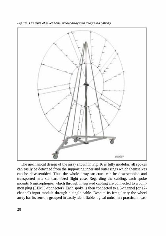
The mechanical design of the array shown in Fig. 16 is fully modular: all spokescan easily be detached from the supporting inner and outer rings which themselvescan be disassembled. Thus the whole array structure can be disassembled andtransported in a standard-sized flight case. Regarding the cabling, each spokemounts 6 microphones, which through integrated cabling are connected to a com-mon plug (LEMO-connector). Each spoke is then connected to a 6-channel (or 12-channel) input module through a single cable. Despite its irregularity the wheelarray has its sensors grouped in easily identifiable logical units. In a practical meas-

Fig. 16. Example of 90-channel wheel array with integrated cabling


29

urement situation, which requires channel detection, calibration and occasionallydetection of hardware faults, this is a great advantage.

A variant of the wheel array is the half-wheel array, intended for measurementsabove a fully reflective ground/floor. In the half-wheel array, the spoke tilt angle iszero because the array design is required to be symmetric with respect to theground floor, Fig. 11(f).

Comparison of the MSL-curves of a wheel array with other arrays with the samechannel count and diameter shows that the wheel array performs better than the tra-ditional regular arrays, Fig. 14. The optimised random array performs slightly bet-ter than the wheel array but, as mentioned above, this type of array is difficult tooperate. Summarising, the wheel array combines high performance with easy oper-ation and manufacturing.

InstrumentationA complete PULSE-based beamforming system consists of the following maincomponents:

• A beamforming array structure with transducers, cabling and optional Webcamera.

• A PULSE front-end system

• PULSE data acquisition software including Data Recorder Type 7701 con-trolled by the Acoustic Test Consultant Type 7761

• A beamforming calculation module Type 7768

• For display of the results, Noise Source Identification Type 7752 is used

A complete configuration list is given in the Product Data for Type 7768.

Beamformer ArraysThere are several possibilities for beamformer array structures, including patentedwheel arrays, traditional cross and grid arrays as well as other irregular array types(logarithmic spirals, Archimedean spirals). For optimal performance, we recom-mend one of our patented wheel types of array: see “Brüel & Kjær Wheel Array”on page 27.

The structures can be full arrays or “half arrays”, where mirror-ground condi-tions can be utilised. A special possibility is flush-mounted microphones, whichcan be beneficial in wind-tunnel applications or at high frequencies to avoid dif-fraction in the microphones and in the support structure.


30

TransducersTwo types of array microphones are ideal for beamforming measurements. ArrayMicrophone Type 4935 is ideal for measurement below 5 kHz, Type 4935-W001extends the frequency range up to 10 kHz, and finally Array Microphone Type4944 A is ideal for measurements up to 20 kHz and for array types with flush-mounted microphones. Both microphone types support IEEE 1451.4 Transducer

Fig. 17. Contour plots showing simulation results of source reconstruction using the arraysdepicted in Fig. 11 applied with different beamforming algorithms. All data sets are normalisedto 0 dB at maximum and the dynamic range is 15 dB. In the simulations, a 5 kHz monopolewas placed in front of the array centre at 1 m distance. (a) and (b) show the results for thecross array, Fig. 11(a), using delay-and-sum and Hanning weighted cross-array beamforming,respectively [“Cross-array Beamforming Algorithm” on page 25]. (c) – (f) show the results ofdelay-and-sum beamforming for the grid array, the optimised random array, the Archimedeanspiral array and the wheel array depicted in Fig. 11(b) – (e). (g) – (i) illustrate the outcome ofapplying cross-spectral beamforming with autospectra exclusion to the optimised randomarray, the Archimedean spiral array and the wheel array, respectively


31

Electronic Data Sheet, which allows automatic transfer of the transducers’ serialnumbers and sensitivity data to be used directly in the application. Calibration canbe performed on six microphones in parallel using the special pistonphone adaptor

Fig. 18. Contour plots showing simulation results of source reconstruction using the arraysdepicted in Fig. 11 applied with different beamforming algorithms. All data sets are normalisedto 0 dB at maximum and the dynamic range is 15 dB. In the simulations, four 5 kHz monopoleswere placed in front of the array at 1m distance. Green asterisks indicate the source posi-tions. (a) and (b) show the results for the cross array, Fig. 11(a), using delay-and-sum andHanning weighted cross-array beamforming, respectively [“Cross-array Beamforming Algo-rithm” on page 25]. (c) shows delay-and-sum beamforming with the grid array, and (d) – (f)give the results of using cross-spectral beamforming with the optimised random array, theArchimedean spiral array and the wheel array. The last row illustrates a mirror-ground situa-tion. (g) represents delay-and-sum beamforming using the cross-array, while (h) and (i) showthe corresponding results for the half-wheel array, Fig. 11(f), using mirror-ground delay-and-sum beamforming (h) and mirror-ground cross-spectral beamforming (i)


32

WA 0728, and the system automatically detects which channels are being cali-brated.

Other transducers such as hydrophones for underwater applications can also beused.

Data Acquisitions System and Beamforming CalculationsData acquisition is performed using PULSE hardware and software. The measure-ment process is controlled by PULSE Acoustic Test Consultant (ATC) Type 7761and involves use of PULSE Data Recorder Type 7701. ATC provides fast and easysetup of multichannel array systems, including automatic channel detection, paral-lel multichannel calibration, real-time level monitoring and on-line determinationof channel status. The measured time data is stored in a PULSE database (based onMicrosoft® SQL Server™), from which it can be retrieved for beamforming calcu-lations using Type 7768.

When searching in large databases, measurements can be identified according touser-defined criteria based on meta-data stored with the measurement data.

From each measurement it is possible to perform multiple calculations, forexample, by focusing on specific parts of the test object or on specific frequencybands. Also, it is possible to choose whether the calculation is performed with thefree-field or mirror-ground algorithm (see Fig. 22 for a screen dump of the Calcula-tion Setup dialog). Three different types of calculations are available: Stationary,Quasi-stationary and Non-stationary. The first two methods are based on the cross-spectral imaging function described in “Cross-spectral Imaging Function” onpage 16. When “Stationary” is selected, the cross-spectra are averaged over theentire selected time interval before being applied in the cross-spectral imagingfunction with autospectrum exclusion, eq. (36). When “Quasi-stationary” isselected, the same procedure is performed in a number of subintervals whereapproximate stationarity can be assumed. This method is useful for the analysis of,for example, slow run-ups where the sound field can be assumed approximatelystationary in narrow RPM intervals. With “Non-Stationary” selected, a time-domain beamforming calculation is performed in the following way: First an FFTis performed on the full selected time record length. Then the near-field Delay-and-Sum algorithm eq. (29) (normalised by the channel count) is applied for each FFTline. Finally, the frequency domain results are converted into time-domain usinginverse FFT. The resulting time data can then be averaged in time intervals or, if atachometer signal has been recorded, in angle-, tacho-, or RPM-intervals.


33

To display the result of a calculation using Noise Source Identification softwareType 7752, simply drag and drop it into a display window. The display windowcontains both a map and a spectral view of the result.

These views are aligned, so the map always represents the frequency rangeselected by a delta-cursor in the spectrum, and the spectrum always shows the datafor the selected cursor point on the map. Additionally, extensive display manage-ment tools are available, including zoom, scroll, tilt, rotate, and animation. Differ-ent calculations can be displayed in separate display windows for comparison, or inthe same display for a complete 3D result.

Practical Aspects of Designing and Using Beamformer ArraysWhen designing an array for beamforming and when performing practical meas-urements, a number of practical aspects must be taken into account. These includethe lower and upper frequency limitations of the array design, the MSL of the arraydefining its dynamic range, the array diameter, the measurement distance, the spa-tial resolution and the size of the mapping area. As will be explained below, thesequantities are highly interconnected. The relations are summarised and illustratedin Table 1.

The Maximum Sidelobe Level (MSL) defines the dynamic range in the ability ofthe array to separate sources in different directions (see “Maximum Sidelobe Lev-els” on page 11). If, for example, the MSL is equal to –12 dB for frequencies up to5 kHz and focusing within an angle of 30° from the axis, then within these limita-tions ghost images of a source in a single direction will always be suppressed by atleast 12 dB relative to the strength of the real source. Other sources, which are not12 dB weaker than the first source, will therefore not be hidden by the ghost imagesof the first source. The MSL is an important parameter when choosing an arraydesign. Conversely, when interpreting results obtained by a given array, it is impor-tant to be aware of its MSL.

The acoustical environment, such as reflections and disturbing sources, must beconsidered when choosing an appropriate array design. A fully reflective floor canbe exploited beneficially by using an array designed for the mirror-ground situa-tion, for example, a half wheel, Fig. 11(f), and by applying a mirror-ground algo-rithm to the recorded signals. Other reflections will significantly disturb themeasurement if the reflected contributions are within the dynamic range of thearray, that is, if they are dampened relative to the direct contribution by less thanthe array’s MSL. Strong disturbing sources or reflections behind a planar arrayshould be avoided, as the array cannot distinguish a source behind the array from


34

its mirror image in the array plane. Sources behind the array will show up in thesource map as image sources located in front of the array.

For many array designs there is no strict upper limit on the usable frequencyrange, because the MSL is slowly increasing with frequency for a given appliedopening angle. In the case of regular arrays, however, the presence of grating lobesimposes a rather strict upper frequency limit. We can illustrate this by consideringthe MSL of the grid array, Fig. 14, with grid spacing d. This MSL-curve shows a

Table 1. Beamformer properties at 30º opening angle

Array

30

z

040029

30

T

040030

Frequency range for chosen threshold T

fmax 30°( ) 43--- fT=

fmin 30°( ) cD----=

Resolution at distance z

Area covered at distance zL = 1.15z

R 1,22 zD----k=


35

sharp cut-off at the spatial angular sampling frequency Ks = 2KN = 2p/d, which fora 90° maximum off-axis focusing angle corresponds to a maximum frequencyequal to fmax(90°) = Kmaxc/4p, see eq. (20). According to eq. (21), the maximumfrequency for 30º off-axis angle is then given by fmax(30°) = (4/3) fmax(90°). For thearray in question, with grid spacing d = 1/7 m, this means that when applied with itsmaximum 90º opening angle, we must restrict ourselves to frequencies belowfmax(90°) = 1.2 kHz, whereas the same array can be used up to fmax(30°) = 1.6 kHzif the maximum off-axis angle is reduced to 30º. The MSL-curve for irregulararrays does not have a sharp cut-off at a well-defined frequency. Instead the MSLdeteriorates gradually with increasing frequency, Fig. 14. In this case, choosing athreshold level T can identify the upper usable frequency fT (Table 1). The thresh-old level, T, should be chosen as the acceptable overall MSL, and in practical meas-urement situations a threshold level of T = –10 dB or lower should be preferred.The threshold frequency fT is then the upper usable frequency at 90º off-axis angle,and at 30º maximum off-axis angle we have:

fmax(30°) = (4/3) fT (42)

The lower usable frequency of a beamformer array cannot be inferred from thearrays MSL-curve. Instead, considerations about the obtainable resolution at finitedistance can give a useful number. A beamformer array relies on the phase differ-ences between the signals recorded by its transducers to determine the angle ofincidence of an incoming sound field. For wavelengths larger than the array aper-ture the phase differences become too small for the beamformer to effectivelyidentify the angle of incidence, and as a consequence the ability to resolve differ-ent sources will be poor. We can determine a minimum frequency, fmin, by therequirement that when applying the beamformer array with a 30º maximum off-axis angle it must be possible to resolve two maximally separated monopoles withfrequency fmin. Here, maximum separation means that the distance between thetwo sources is 2tan(30°)z ≈ 1.15z which is the linear size of the focus area at dis-tance z for an opening angle of 30º around the axis. Then, referring to eq. (15) witha = 1.22, the lower frequency for an array with diameter D is determined from1.15z = 1.22(z/D)[c/fmin(30°)], or

fmin(30°) ≈ c/D (43)

In many cases, however, the resolution will be too poor at frequencies as low asgiven by eq. (43).


36

Application ExamplesThe application examples given in here represent noise source location problems,where beamforming is an attractive measurement method.

A Vehicle in a Test HallThe first example is measurement of the noise radiation from a complete vehicle.At high frequencies a complete vehicle will be much larger than the wavelength,meaning that Near-field Acoustical Holography (NAH) will require a hugenumber of measurement points. For the cases when the vehicle is operated in asteady state on a dynamometer drum in a test hall, a scanning technique – such asSTSF – could be used to measure all these positions with a realistic microphonearray. The measurement time will, however, be significant, and there will be prob-lems such as stationarity and reference selection. For the case of run-up operatingconditions (simulated pass-by), a scanning technique is not easy to use: RPMinterval averaging will typically have to be used, and quasi-stationarity will haveto be assumed in each interval, which is a problematic assumption. The mainadvantages of NAH (STSF) are:

• High resolution on the source plane – also at low frequencies

• Possibility to simulate source modifications on the source plane. For exam-ple, this enables contribution analysis in any far field position

• Source ranking based on calibrated intensity maps

Beamforming, on the other hand, provides the possibility of doing a broad-banded,one-shot measurement with an irregular array at some intermediate measurementdistance, typically 3 –7 m. The directional contribution maps obtained from such ameasurement will show the positions of the noise-radiating regions with the high-est relative contributions to the noise at the array position. No calibrated sourcedescriptor such as sound power can be achieved, however.

Since a Test Hall has a reflecting ground plane, it is obvious to measure with ahalf-wheel array.

A Vehicle in a Wind-tunnelFor measurements on a vehicle in a wind-tunnel, there are many similarities withmeasurements in a test hall: there is a reflecting ground plane allowing the use of ahalf-wheel array, and the source will be much larger than the wavelength at highfrequencies. An additional condition is that measurements have to be taken atquite long distances to stay out of flow. This is natural for beamforming, butwould further increase the size of the measurement area for NAH (STSF), and at


37

such large measurement distances NAH loses its ability to provide good low-fre-quency resolution. To maintain good low-frequency resolution with NAH, a moredifficult in-flow scanning of a microphone array is required.

The 90-channel wheel array of Fig. 16 has been used to perform a measurementon a car in a wind tunnel. This array has a diameter of 2.4 m and provides low MSL(–14 dB) up to 3 kHz with 90° maximum off-axis angle and 4 kHz with 30° maxi-mum off-axis angle. An alternative NAH measurement, also covering the fre-quency range up to 3 kHz, would require in-flow scanning of a microphone arrayover a grid covering the car side with a grid spacing not larger than 5 cm. Thebeamforming measurement is a simple “one-shot” recording taken with the 90-ele-ment array outside the flow region.

The vehicle was centred in the flow section, facing the wind, and the wind speedwas set to 130 km/h. The wheel array was placed parallel to the side of the car at adistance of 3.3 m. The stationary beamforming calculation shown in Fig. 19 clearly

Fig. 19. Car in a wind-tunnel at 130 km/h wind speed


38

reveals noise radiation from the front wheel, the side mirror, the A-pillar and thedoor handle in the frequency interval from 2.1 kHz to 2.6 kHz. The spectrum plotrepresents the contour cursor position on the door handle, and the contour plot rep-resents the frequency interval selected by the delta cursor in the spectrum plot. Forthis application, a low MSL (a large dynamic range) is very important to preventghost images from the strong radiation around the wheel to mask the other sources.

A Large Source (Crane)Beamforming is a very powerful technique for noise source location on largesources up to rather high frequencies, requiring only a single recording with amicrophone array. In this example, a 42-channel wheel array with a diameter of1 m was positioned 7 m from a crane hoisting at maximum load, see Fig. 20. Thearray, the geometry of which is shown in Fig. 15, has MSL below –10.6 dB up to4.8 kHz for 90° maximum off-axis angle and up to 6.4 kHz for 30° maximum off-

Fig. 20. Mobile crane hoisting at maximum load


39

axis angle. The rather long measurement distance was chosen in order to get alarge mapping area, at the sacrifice of resolution. According to the overview inTable 1, the size of the mapping area can be up to 1.15 × 7 m ≈ 8 m within the 30°maximum off-axis angle, but the resolution will be only 1.22 × 7/1 ≈ 8.5 wave-lengths.

Fig. 20 shows the source location for a frequency band around 2.05 kHz, wherethe spectrum shows a peak. The spectrum represents an area of high-level radiationover a cover plate that is probably resonating within the selected frequency band.

An Engine at High FrequenciesThis example is a measurement on a car engine with a 66-element, 1 meter diame-ter wheel array. This wheel array has MSL below –10.4 dB up to 16 kHz with 90°maximum off-axis angle. The array was hanging approximately 0.9 m over anopen engine compartment, with the engine running at 3500 RPM, and a singletime history recording was made with a frequency bandwidth of 12.8 kHz. Fig. 21contains the result of a Stationary beamforming calculation for the 6.3 kHz, 1/3-octave band, the contour interval being 1 dB.

Fig. 21. Averaged 6.3 kHz, 1/3-octave band for a car engine


40

A NAH measurement covering the frequency range up to, for example, 8 kHzwould require measurement over a regular rectangular grid of points with spacingaround 2 cm. To cover the entire engine compartment would require approximately2500 measurement positions, which should be compared with the 66 positions usedby the beamformer. One major difference between the two techniques is that NAHcan provide calibrated maps of Sound Intensity, Pressure and Particle Velocityclose to the source, while with beamforming one can only get contour plots show-ing relative contributions to the sound field at the array position. No calibratedabsolute levels near the source surface are obtained with beamforming.

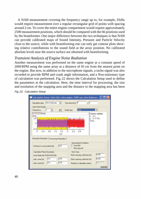
Transient Analysis of Engine Noise RadiationAnother measurement was performed on the same engine at a constant speed of2000 RPM using the same array at a distance of 81 cm from the nearest point onthe engine. But now, in addition to the microphone signals, a tacho signal was alsorecorded to provide RPM and crank angle information, and a Non-stationary typeof calculation was performed. Fig. 22 shows the Calculation Setup used to definethe parameters in the calculation. Here, the time interval for processing, the sizeand resolution of the mapping area and the distance to the mapping area has been

Fig. 22. Calculation Setup


41

defined. Under the tab page named Processing Parameters, the frequency rangeand type of averaging have been chosen. In this case we have used 1/3-octaveband filters and performed (crankshaft) Angle Interval averaging in intervals of 5°.Thus, for each 1/3-octave band we get 720/5 = 144 maps of the radiation during anengine cycle consisting of two revolutions. For each angle interval, averaging hasbeen performed over all rotations within the selected time interval.

When doing angle interval averaging, one has to be aware of the time smearingperformed by the impulse response of the frequency band-pass filters used. With afrequency bandwidth equal to B, the impulse response will have duration around1/B. This should be related to the time for one rotation, which is 60 s/RPM. Animpulse will therefore be smeared over an angle of approximate width 6° · RPM/B.For the present measurement we shall be looking at data for the 3.15 kHz, 1/3-octave band, and the smearing angle turns out to be approximately 15°.

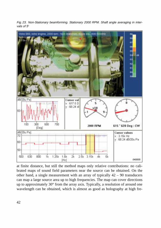
A typical result is shown in Fig. 23. The angle meter shows a crank angle intervalfrom 615° to 620° and the spectrum plot shows that only the 3.15 kHz, 1/3-octaveband has been selected for mapping. The spectrum represents the cursor positionon the peak of the contour plot. Clearly, the 3.15 kHz, 1/3-octave band is verystrong at the chosen peak position. To the left of the Angle (and RPM) meter, thevariation with angle at the cursor position is plotted. The sharp peaks indicate thatthe radiation at the peak position is very impulsive and concentrated at a few dis-crete shaft angles.

Another typical type of analysis would be averaging in RPM intervals for run-upmeasurements.

For the present measurement, we used only a single tacho signal providing a sin-gle impulse per cycle (of two revolutions). This provides a unique identification ofa reference angular position during each cycle, but it does not necessarily allow anaccurate estimation of the angle during the entire cycle. For this, the system sup-ports the use of a second high-resolution tacho signal.

ConclusionsBeamforming is a noise source location method based on measurements with aplanar array of microphones or hydrophones at an intermediate distance from thesource. The beamforming calculation can then basically resolve the relative contri-butions from different directions to the sound field seen by the array. Pure direc-tional resolution would correspond to focus at infinite distance. Ourimplementations always focus on a source plane parallel with the array plane, i.e.,


42

at finite distance, but still the method maps only relative contributions: no cali-brated maps of sound field parameters near the source can be obtained. On theother hand, a single measurement with an array of typically 42 – 90 transducerscan map a large source area up to high frequencies. The map can cover directionsup to approximately 30° from the array axis. Typically, a resolution of around onewavelength can be obtained, which is almost as good as holography at high fre-

Fig. 23. Non-Stationary beamforming. Stationary 2000 RPM. Shaft angle averaging in inter-vals of 5°


43

quencies, but at low frequencies holography can do much better. At very high fre-quencies, on the other hand, where holography is not feasible because of therequired half-wavelength microphone grid spacing, beamforming can providehigh resolution with relatively few measurement points.

The basic principle of beamforming has been outlined, and the performance ofdifferent array designs has been analysed and compared. The wheel array design,which is patented by Brüel & Kjær, has been shown to offer some distinct advan-tages: a combination of high performance and ease of handling. A new, self-term-free, cross-spectral beamforming algorithm has been described and shown to offer:(i) suppression of noise in the individual measurement channels, (ii) suppression ofsidelobes (and thus of ghost images) and (iii) a natural distance correction for theindividual array transducers when the array is used at a finite distance. The meas-urement system has been described together with guidelines for design and use ofthe system, and finally some typical application examples have been presented.

Appendix: The Cross-spectral Imaging FunctionIn this appendix we derive the Cross-spectral Imaging function applied in PULSEStationary Beamforming. For each position on the source plane, the estimatedsource strength reflects how well the sound field from a monopole point source atthat position fits the sound field measured by the array. The approach is inspiredby reference [9].

The error function defined in eq. (34):

(A.1)

can be written in a form that is convenient for the derivations, if we stack all thecolumns of the cross-spectral matrix [Cnm] in a single-column matrix, and arrangethe elements [vn

*vm] in a similar matrix:

(A.2)

For each position r, we first determine the monopole strength â that minimisesthe error function, eq. (A.1). To do this we notice that the error function is mini-

E a r,( ) Cnm Cmodnm–

2Cnm av*

nr( )vm r( )–

2

m n, 1=

M

∑=m n, 1=

M

∑=

g Cnm[ ]=

h r( ) v*n

r( )vm r( )=


44

mised by least squares solution of g ≈ ah, which upon multiplication from the leftwith h† leads to:

(† transposed complex conjugate) (A.3)

Appealing to the fact that the cross-spectral matrix is Hermitian and to the defini-tion (A.2) of h and g, we see that h†g is real and equal to g†h. Therefore â is alsoreal.

Use of eq. (A.2), eq. (A.3) and the relation g†h = h†g in eq. (A.1) leads to the fol-lowing expression for the error function:

(A.4)

Minimising the error function over all r thus corresponds to maximising the Imag-ing Function, I(x, r),

(A.5)

over all r (we choose the definition I4 since eq. (A.5) has units of power squared).In practice I(x, r) is computed over a discrete mesh covering the focus area. In theresulting map, peaks are interpreted as areas with a high probability of finding asource. This interpretation can be justified if we compare the imaging function inthe far field with the corresponding expression for the Delay-and-Sum beam-former, eq. (7). For large R ≡ |r| the approximation |rm – r| ≡ Rm ≈ R is valid in con-nection with the amplitude of vm(r) ≡ v(rm – r). In the far-field limit eq. (A.5) cantherefore be approximated by:

a r( ) h†g h

†h⁄=

E a r,( ) g ah r( )–2

g†g a h

†g g

†h+( )– a

2h

†h+ g

†g

h†g( )

2

h†h

----------------–= = =

I4

x r,( )h

†g( )

2

h†h

---------------- =

Cnm x( )vn r( )v*m

r( )m n, 1=

M

∑2

vn* r( )vm r( )

2

m n, 1=

M

∑-----------------------------------------------------------------------≡


45

(A.6)

Expanding the square of eq. (7) and taking the average we find:

(A.7)

where we have used that the difference in travel paths Rn – Rm equals the projec-tion difference �⋅(rm – rn), Fig. A1. Obviously, we have:

I2/M =

which shows us that the imaging function in the far field, when normalised by thechannel count, equals the output of the Delay-and-Sum beamformer. This observa-tion justifies the chosen interpretation. The normalisation factor has been includedin eq. (35).

Fig. A1. For a source in the far field, the difference, Rn – Rm, in the propagation path length tothe transducers at rn and rm can be calculated from the diagram

I4

R4

Cnmvnv*m

m n, 1=

M

∑2

R4

vn* vm

2

m n, 1=

M

∑----------------------------------------------------

CnmejkRn–

ejkRm

m n, 1=

M

∑2

ejkRn–

ejkRm 2

m n, 1=

M

∑--------------------------------------------------------------≈=

1

M2

------- Cnmejk Rn Rm–( )–

m n, 1=

M

∑2

=

B2 1

M2

------- Pn* Pme

jk� rm rn–( )–

m n, 1=

M

∑ 1

M2

------- Cnmejk Rn Rm–( )–

m n, 1=

M

∑= =

B2

�·

�·

Far field source

040028

�


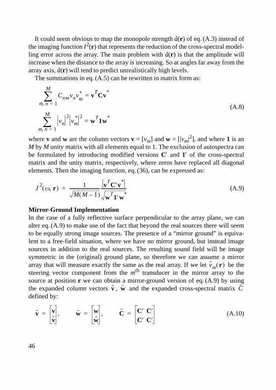
46

It could seem obvious to map the monopole strength â(r) of eq. (A.3) instead ofthe imaging function I2(r) that represents the reduction of the cross-spectral model-ling error across the array. The main problem with â(r) is that the amplitude willincrease when the distance to the array is increasing. So at angles far away from thearray axis, â(r) will tend to predict unrealistically high levels.

The summations in eq. (A.5) can be rewritten in matrix form as:

(A.8)

where v and w are the column vectors v = [vm] and w = [|vm|2], and where 1 is anM by M unity matrix with all elements equal to 1. The exclusion of autospectra canbe formulated by introducing modified versions C′ and 1′ of the cross-spectralmatrix and the unity matrix, respectively, where zeros have replaced all diagonalelements. Then the imaging function, eq. (36), can be expressed as:

(A.9)

Mirror-Ground ImplementationIn the case of a fully reflective surface perpendicular to the array plane, we canalter eq. (A.9) to make use of the fact that beyond the real sources there will seemto be equally strong image sources. The presence of a “mirror ground” is equiva-lent to a free-field situation, where we have no mirror ground, but instead imagesources in addition to the real sources. The resulting sound field will be imagesymmetric in the (original) ground plane, so therefore we can assume a mirrorarray that will measure exactly the same as the real array. If we let be thesteering vector component from the mth transducer in the mirror array to thesource at position r we can obtain a mirror-ground version of eq. (A.9) by usingthe expanded column vectors , and the expanded cross-spectral matrix defined by:

(A.10)

Cnmvnv*m

m n, 1=

M

∑ vT

Cv*

=

vn

2vm

* 2

m n, 1=

M

∑ wT

1w*

=

J2

x r,( ) 1

M M 1–( )---------------------------- v

TC′v*

wT

1′w*-----------------------=

vm r( )

v w C

v vv

,= w ww

,= C C′ C′C′ C′

=


47

The cross-spectral imaging function for the mirror-ground situation is then:

(A.11)

The normalising factor is here 2M(2M – 2), since now 4M elements out of 4M2 in equal zero, and is constructed from 1′ exactly as is constructed from C′.

Appendix: ResolutionWith reference to Fig. 5, we can evaluate the resolution as follows. As stated in“Resolution” on page 8, two incident plane waves of equal amplitude with wavenumber vectors k1and k2, |k1| = |k2| = k, can be resolved only if the projections and of k1 and k2 on the array plane are not within RK = Kmin

0 from each other.Here, RK is the main-lobe width in the array pattern W(K), and Kmin

0 is the posi-tion of the first minimum of the array pattern. In Fig. 5 we have

so the two plane waves are just exactly resolvable.In the focus plane, we shall look only at the resolution in the radial direction, that

is, in the direction away from the array axis. We choose to look at the resolutionalong the x-axis. The plane wave with wave number vector k1 is incident at anangle h from the array axis, and the exactly resolvable plane wave with wavenumber vector k2 is incident at an angle h +Rh from the axis, Rh being the angularresolution in the radial direction. These two directions span the resolution R alongthe x-axis at the distance z from the array plane (on the focus plane).

In the derivation we will now assume a very fine resolution, meaning that we canconsider the resolutions in K, h and x to be differential: RK = dK, Rh = dh and R =dx. From K = ksin(h) we get dK = kcoshdh and therefore:

From the relation x = z tg(h) we get:

and combination of the two above relations leads to:

J2

x r,( ) 1

2M 2M 2–( )----------------------------------- v

TCv

*

wT

1w*

----------------------=

C 1 C

k1k2

k2 k1– RK=

dh dKk hcos--------------=

dx z dh

cos2h

-------------=


48

Finally, we replace the differential resolutions with the real finite resolutions andget:

References[1] Maynard J.D., Williams E.G. and Lee Y., “Nearfield acoustical holography:

I. Theory of generalized holography and the development of NAH”, J.Acoust. Soc. Am. 78(4), 1985, pp. 1395 – 1413.

[2] Hald J., “STSF – a unique technique for scan-based Near-field AcousticHolography without restrictions on coherence”, Brüel & Kjær TechnicalReview No. 1, 1989, pp. 1 – 50.

[3] Johnson D. H. and Dudgeon D. E., “Array Signal Processing: Concepts andTechniques”, Prentice Hall, New Jersey, 1993.

[4] Proakis J.G. and Manolakis D. G., “Digital Signal Processing, Principles,Algorithms, and Applications”, 3rd Edition, Prentice Hall, New Jersey,1996.

[5] Yasushi Takano, “Two-dimensional Microphone Array System for Measur-ing Distribution of Aerodynamic Noise-sources on High-speed Trains”,International Symposium on Simulation, Visualization and Auralization forAcoustic Research and Education, Tokyo, 1997

[6] Underbrink J. R. and Dougherty R. P., “Array Design for Non-intrusiveMeasurement of Noise Sources”, Proceedings of Noise-Con 96, pp. 757 –762, 1996.

[7] Nordborg A., Wedemann J. and Willenbrink L., “Optimum Array Micro-phone Configuration”, Proceedings of Internoise 2000.

[8] Danish patent No. PA 2002 00412.

[9] Elias G., Proceedings of Internoise 1995, pp.1175 – 1178.

dx z dKk

----------- 1

cos3h

-------------=

Rz RK

k----------- 1

cos3h

-------------≈


2 – 1988 Quantifying Draught Risk1 – 1988 Using Experimental Modal Analysis to Simulate Structural Dynamic

ModificationsUse of Operational Deflection Shapes for Noise Control of Discrete Tones

4 – 1987 Windows to FFT Analysis (Part II)Acoustic Calibrator for Intensity Measurement Systems

3 – 1987 Windows to FFT Analysis (Part I)2 – 1987 Recent Developments in Accelerometer Design

Trends in Accelerometer Calibration1 – 1987 Vibration Monitoring of Machines4 – 1986 Field Measurements of Sound Insulation with a Battery-Operated Intensity

AnalyzerPressure Microphones for Intensity Measurements with Significantly Improved Phase PropertiesMeasurement of Acoustical Distance between Intensity Probe MicrophonesWind and Turbulence Noise of Turbulence Screen, Nose Cone and Sound Intensity Probe with Wind Screen

3 – 1986 A Method of Determining the Modal Frequencies of Structures with Coupled ModesImprovement to Monoreference Modal Data by Adding an Oblique Degree of Freedom for the Reference

2 – 1986 Quality in Spectral Match of Photometric TransducersGuide to Lighting of Urban Areas

1 – 1986 Environmental Noise Measurements

Special technical literatureBrüel & Kjær publishes a variety of technical literature which can be obtained from your local Brüel & Kjær representative.

The following literature is presently available:

• Catalogues (several languages)• Product Data Sheets (English, German, French,)

Furthermore, back copies of the Technical Review can be supplied as listed above. Older issues may be obtained provided they are still in stock.

Previously issued numbers of Brüel & Kjær Technical Review(Continued from cover page 2)


TECHNICAL REVIEW

Beamforming

HEADQUARTERS: DK-2850 Nærum · DenmarkTelephone: +45 4580 0500 · Fax: +45 4580 14 05www.bksv.com · [email protected]

BV

0056

–11

ISSN

000

7–26

21

No.1 2004

BV0056-11_TR_Cover2004.qxd 23-03-2004 13:33 Page 1

Documents

BV0056-11 TR Cover2004.qxd 23-03-2004 13:33 Page 1 ...Vibration Measurement A/S, DK-2850 Nærum, Denmark. Editor: Harry K. Zaveri bv005611.book Page iii Tuesday, March 23, 2004 12:46