POLITICAL DEVOLUTION WITHOUT FISCAL DEVOLUTION

by

Andrew Hughes Hallett

Working Paper No. 05-W05

March 2005

DEPARTMENT OF ECONOMICSVANDERBILT UNIVERSITY

NASHVILLE, TN 37235

www.vanderbilt.edu/econ

1

Political Devolution without Fiscal Devolution A Federalist Paper on Tax Harmonisation, Regional Budgets, and

Local Market Flexibility∗

Andrew Hughes Hallett Vanderbilt University and CEPR

Abstract: Using a conventional model, this paper examines the conditions under which it is possible to stabilise both the output (inflation) cycle and the budget deficit/surplus of a regional economy in a wider currency union. We find that it is never possible. But we can approximate that result (for example, by limiting budgetary instability when the cycle is smoothed) if the product and labour markets are suitably flexible. Conversely, if fiscal policy is restricted, output and inflation volatility will be extended unless all shocks are supply shocks, compared to the case where there is some fiscal autonomy. Attempts at stabilisation in this situation would lead to an unstable political equilibrium. These results are important because they show what can be expected from fiscal restraints like the Stability Pact or tax harmonisation in the Eurozone; and from fiscal autonomy at the subnational level in older unions. Calibrating the results for the EU and UK respectively, we find that denying autonomy to the regions of the UK might be rather costly in terms of performance. But imposing tax harmonisation at the EU level would not.

JEL Codes: E32, E63, R13

Keywords: Business cycle volatility, budget stability, regional autonomy, market flexibility

March 2005

∗ I am very grateful to the Devolution Programme of the UK Economic and Social Research Council (grant no. L219252122) for financial support during the preparation of this paper.

2

1. Introduction This paper asks under what circumstances can a regional economic cycle be smoothed without the local budget deficit being destabilized or expanded? It is assumed that the region enjoys a measure of political devolution: that is, some political focus exists where the state of the local economy can be discussed, and institutions exist which allow estimates of the region’s GDP, employment, fiscal balance (including the net subsidy to/from others) to be calculated. We also assume that the region has no direct access to a monetary policy of its own. That monetary policy is chosen by a union-wide Central Bank for the union to which this region belongs. Monetary policy is therefore directed at a common inflation rate; where arbitrage exists in the goods market, together with a common currency and no trade barriers. Monetary policy could also be used to reduce the average output gap in a multilateral currency union, but not in a unilateral one. That distinction is important.

This set-up defines the economic side of political devolution if no power over instruments for managing the local economy is granted to the local authority. We can then examine the outcomes, in terms of the regional cycle and budgetary balances, when the region is granted its own tax raising or spending powers (fiscal devolution), compared to when it is not (no fiscal devolution; the union-wide parameters apply). We can also see what happens when the degree of fiscal autonomy is increased or decreased.

It is important to ask such questions because most political and currency unions grant some fiscal autonomy to their regional economies, but they vary a great deal in how much they allow. It is almost total in the Eurozone1. And it is significant in Canada, the US, Switzerland, Australia, India and some Latin American economies. But others have political devolution with either no fiscal devolution (France, Italy2, the UK); or only limited fiscal devolution (Spain, Germany). In any of these cases it would be interesting to know if strengthening the degree of fiscal autonomy could reduce the regional cycles without destabilising the budget. Or, equivalently, how much the cycle would be exaggerated if the stabilising effect of a local fiscal policy were suppressed.

In analyzing questions of this kind, the key point is that the budget itself is endogenous. In fact, the automatic stabilising action of fiscal policy consists of two parts: (1) the stabilising effects of changing tax yields and social expenditures which vary counter-cyclically; and (2) the destabilising effects of those counter-cyclical movements on the budget balance itself. These two components are not independent of one another. Stronger automatic stabilisers would stabilise the cycle more, and may therefore help preserve stronger revenues and smaller expenditures in a downturn. But they would certainly take more out of the budget to do so. Conversely, stronger automatic stabilisers in a boom might mean weaker revenues and lager expenditures than otherwise – but would put more into any emerging surplus.

Whether the budget is then net stabilised or net destabilised depends on whether the stabilising effect on the cycle is stronger than the destabilising effect on the budget. That is, on whether the direct effect of the budget on the cycle is larger than the direct and indirect effects of cyclical income changes on the budget. There may be 1 The limits of the Stability Pact apart. 2 With the exception of the autonomous regions: Sicily, Aosta and South Tyrol.

3

circumstances when it is. But it may also be that the multipliers on the cycle are smaller than the multipliers on the budget. In that case it won’t be possible to stabilise both the cycle and the budget together; and we will have to choose between having the cycle stabilised to within certain limits vs. having the budget stabilised within certain limits. This paper therefore first determines the conditions under which such choices have to be made. We then show that these choices depend on the degree of deregulation or supply side flexibility in the regional economy. The role of union-wide policy making in this choice is minimal.

2. Can We Stabilise Both Regional Budgets and Regional Business Cycles with Stronger Automatic Stabilisers? Consider a simple aggregate demand/aggregate supply model of a small open regional economy within a larger union:3

ded yidy εφπφπφφ +−−−−= 4321 )( (1)

sesy εππω +−= )( (2)

This regional economy will be one part of a larger economic union with a common currency. All variables will therefore be defined as deviations from their union wide counterparts; and output a deviation from its long run trend. The output cycle will then be measured relative to the cycle of the union. Inflation will likewise be measured as short term deviations from the union average; and the budget variables, as deviations from some pre-existing budget position at the regional level. The union budget doesn’t have to be in balance therefore, and the regional government (where it has devolved power) is not responsible for its implicit share of the union budget – only for its own budget, or for its direct contribution to the consolidated budget. Equally that union budget will not be specifically chosen to stabilise, or otherwise aid the regional economy – beyond whatever is necessary to stabilise or provide public services for the union as a whole.

We can now set about tracking the development and stability of the regional budget, output cycle and inflation around their union-wide counterparts when the regional government is, and is not, allowed to operate its own fiscal policies to stabilise its own economy relative to the union average. Two regimes are considered. First the regional government may only choose local tax rates and local expenditure shares: i.e. it has to rely on automatic stabilisers. But it may choose how strong those stabilisers should be. This is a restriction which ensures that the regional budget will come back to balance 3 Despite its simplicity, this is a model widely used for analysing problems of this kind: Blanchard 2000; Brunilla et al 2003. Its derivation from underlying economic behaviour is given by Artis and Buti (2000). Coenen and Wieland (2002) meanwhile argue that bilateral interactions with other economies can be ignored at this level of abstraction. It is also the model used by Akerlof, Dickens and Perry (2000), Ball (1999), Rudebusch and Svensson (1999), Svensson (1997) and Bean (1998) if policy lags are suppressed, fiscal policy is added and their separate equations for π and y are combined. Finally Martin and Rowthorn (2004) use it to track changes in economic stability, which is the issue at stake this paper, and show that it allows for both competitive and imperfectly competitive firms. In this paper, we generalise the model yet further by allowing market based expectations, and hence inflation surprises, to be part of the story.

4

whenever the union economy is in equilibrium and the regional economy has reached the union average4. Second, we can allow the regional government to make discretionary expenditures or savings as well. That is a more generous fiscal regime and clearly carries the potential for providing greater regional stabilisation -- as well as larger, more unstable deficits. In either case, the absence of fiscal devolution means that both the autonomous elements of regional policy, and the automatic stabilising components subject to regional choice, have been removed.

Note, we do not go on to examine the consequences of adopting different fiscal regimes or different automatic stabilisers at the union level in this paper, although those choices will clearly also have an effect on the overall stability of the region. Since they are not chosen with the region’s economic performance in mind, they will be represented as exogenous shocks to the regional economy in what follows.

2.1 Rule Based Budgets (Regime 1):

Equation (1) is an IS-curve in which aggregate demand, yd, depends on the budget deficit as a proportion of GDP d; the real interest rate (i-πe)); and a demand shock, εd. Assuming our region to be small compared to the rest of the currency union, there will be no significant impact from this economy on the union as a whole. But yd will be affected by domestic competitiveness relative to the rest of the union, φ 3π, and by domestic absorption (persistence), φ 4y. We take all parameters to be positive.

Equation (2) is a supply function, where supply, ys, depends on inflation surprises (π-πe) and a supply shock εs. Fiscal responses or automatic stabilisers however, usually increase with the size of the government sector, the size and progressivity of the tax base, the generosity of the social support and unemployment benefit programmes5 – and with the sensitivity of social or unemployment benefits to the state of the cycle. Hence, we write:

ayd +−= α where )( gt −=α (3)

Here t represents the average tax rate, and g is total government expenditures as a share of GDP. If we wish to see how the economy will perform when automatic stabilisers are allowed to play freely, the discretionary part of policy may be ignored (a = 0). Then, to increase the automatic stabilising effects in a recession, we have to set ∆α< 0 (so that t falls and/or g rises in a recession when y < 0). But to increase the automatic stabilisers (and rainy day funds) in a boom, we must have α∆ > 0 when y > 0. In practice, these effects will come from the progressivity of the tax and benefits system; or from the non-linear effects of subsidies and profit taxes; or from changes in the tax base around the cycle.

Lastly we assume that the monetary authorities set interest rates to eliminate inflation (and perhaps output gaps), using some form of a Taylor rule:

4 The regional budget would not balance if either condition failed because y, in (3), is a deviation from its union counterpart; both are deviations from their respective trends; and those trends may differ (given a=0). 5 See HMT (2003) for numerical estimates of these effects in the European economies.

5

)( yi βπλ += (4)

There are two parameters here: λ indicates the general level of activism, while β ≠ 0 implies that monetary policy reacts (albeit in a small way) to the relative regional output gap. That is possible, but not assured, in a multilateral monetary union. But it would definitely not be the case in a unilateral one. In that regime, β = 0.

2.2 Output and Budgetary Sensitivity to the Automatic Stabilisers

Now we can solve the model. Using (1)-(4), the equilibrium expected rate of inflation is zero: .0=eπ That implies

[ ],)( 32 sdy εφλφωεµ ++= (5a)

and ])1([ 241 sd ελβφφαφεµπ +++−= (5b)

are the realisations of output and inflation, where µ = 1/(ω(1+αφ 1+φ 4)+φ 2λ(1+βω)+φ 3). But since 0)/1(1 <− µαωφ by definition, we also have

[ ][ ] 0)/1()( 1322 >−++=

∂∂ µαωφεφλφωεµα sdd (6)

and [ ] ,0)( 1322 >++−=

∂∂ ωφεφλφωεµα sdy (7)

if .0)( 32 <++ sd εφλφωε The latter would hold if εd / εs < -(φ 2λ +φ 4)/ω when εs > 0; or if ωφλφεε /)(/ 32 +−>sd when sε < 0. Under either of these conditions, and irrespective of the value of β, increasing the automatic stabilisers in a slump (i.e. setting ∆α < 0 when y < 0) will lead to smaller deficits, but larger cycles. Similarly, increasing them in a boom (∆α > 0 when y >0) will reduce the deficit/increase a surplus, but produce larger cycles.

But since sε and dε can be either positive or negative, the opposite inequality can also be true – implying (6) and (7) would be negative. In that case, increasing the automatic stabilisers in a slump would lead to larger deficits, but smaller cycles; and, conversely, to larger surpluses but smaller cycles in a boom6. Thus, with stronger automatic stabilisers, we should expect either stabilised national incomes, or stabilised budgets – but not both. This is because (6) and (7) always share signs.

The lesson from this model is that the case for having stronger automatic stabilisers is not straight forward. In fact the strength of the automatic stabilisers has rather little to do with the ability of fiscal policy to damp the cycle, or with the size of deficits and surpluses needed to do so. In reality, since any stabilisation of the cycle will always be accompanied by a destabilisation of the budget and vice versa, the best that we can hope for is greater stability in the cycle with a limited destabilisation (or deterioration) in the budget; or a stabilisation of the budget with a limited destabilisation of the cycle. But we cannot get both smaller budget deficits and smaller cycles. 6 Larger surpluses mean larger “rainy day funds” against future deficits, but smaller booms in good times. Stronger stabilizers therefore get us either larger rainy day funds, or a damped cycle, but not both.

6

In that case, to get greater cyclical stability with a limited destabilisation of the budget in a slump (y<0), we need the derivatives in (6) to be smaller than those in (7) since having stronger stabilisers means ∆α < 0 in that case. However, a cyclical downturn almost certainly means 0<dε and sε ≤ 0. Hence, to have (6) less than (7) implies

φ 1 >1+φ 4+βλφ 2+ (φ 2λ+φ 3)/ω (8)

has to hold for all such shocks. In other words, the budget multipliers must be large enough if we are to get more cyclical stability than budget instability. And the same inequality must also apply for small but positive supply shocks such that

s0 ε≤ < )/( 32d φλφωε +− when dε <0.

Conversely, in a boom period (y>0), stronger stabilisers mean ∆α > 0. In that case, greater cyclical stability requires (6) to be larger than (7). But that changes nothing since dε > 0 and most likely sε ≥ 0 in this case. Indeed we will require the same inequality, (8), to hold once again so long as

)/( 32d φλφωε +− < sε

holds whenever dε >0.

2.3 The Importance of Market Flexibility

We can make the same points in a more dramatic way. Once we know whether a particular set of automatic stabilisers will tend to increase or decrease the cycle, we can see from (6) and (7) that the margin by which ∂y/∂α fluctuates more than ∂d/∂α does (that is, the degree of extra cyclical stability that we get per unit extra budget instability) will be increased if (ωεd +(φ 2λ+φ 3) sε )µ2 becomes larger in absolute value. For a slump, that means that each εd<0 must be matched with a self-induced negative or sufficiently small positive supply response. That would require some relative prices to fall or layoffs, or stockpiling and reductions in investment, to reduce capacity as the markets adjust to meet the new demand conditions. Similarly, in a boom, we would need to have markets adjust so that each positive demand shock is matched by a positive (or sufficiently small negative) response on the supply side.

In other words, we will only get a smaller output cycle with a less than corresponding increase in the deficit, and hence the possibility of savings for a rainy day in the upturn, if markets – and the labour markets in particular – are sufficiently flexible.

2.4 Alternative Regimes: A Conservative Central Bank and Unilateral Monetary Unions

It is entirely possible that monetary policy will not react to the regional output gap unless its underlying output trend is quite different from the union average. That would certainly be the case if the common Central Bank was very conservative or the region already enjoyed significant fiscal autonomy. It would also be true if the region was small, or if it were a country in a unilateral union with a larger neighbour. We can accommodate these

7

cases by letting β→0. Does this make the regional deficits worse, or the case for fiscal devolution stronger?

Setting β = 0 above, we get

))1(/(1ˆ 3241 φλφφαφωµ ++++= > µ.

in (5a,b). Hence y and π react more to shocks. In addition, it is easy to show that µα ∂∂∂∂ /)/d( >0 and µα ∂∂∂∂ /)/y( >0 under the conditions specified in section 2.2.

Hence reducing β will mean larger budget and output cycles, all other parameters as before. Nevertheless, it will become easier to satisfy the inequality at (8). Consequently we are more likely to get cyclical stability with only a limited destabilisation of the budget than we were before, although that holds because we are starting from a higher level of instability in both y and d. Similarly, market flexibility becomes more important, and for the same reason, because the term involving 2µ in section 2.3 becomes larger.

The same points also apply if the Central Bank becomes less activist (λ→0). The term in section 2.3 gets larger because 2µ is larger, but becomes smaller because the rest of the expression is reduced. Which effect dominates then depends on the shocks. If demand shocks dominate, then market flexibility becomes less important (boom or slump) and the outcomes more dependent on the union itself. But if supply shocks dominate, then it may be that market flexibility is more important (and union policies less important). The lesson here is that the traditional lament of conservative Central Bankers – that regional disequilibria are better corrected by market adjustments – is not always correct. It depends on the type of shock. With demand shocks there is a role for fiscal policy, whether from the centre or locally. That may also be true for supply shocks; or it may not. But in either case, when policies are applied, they need to be applied symmetrically around the cycle.

3. No Fiscal Devolution: the Case of Weaker Automatic Stabilisers The outcomes for a system with no fiscal devolution can be calculated by considering what would happen if there were no regional automatic stabilisers, so that the regional economy has to accept the fiscal policies chosen for the union as a whole. In our context, that means sending α, the region specific fiscal parameter, to zero.7 Does that destabilise the size of any budget deficits, and reduce the possibility of rainy day surpluses? What happens to the output cycle and inflation, relative to the devolution case?

3.1 The Output Cycle

For this case, write output and inflation when fiscal devolution is available as yα and πα. Their values are given in (5). The corresponding values, when no fiscal devolution is permitted, are: 7 We are suppressing regional fiscal policies only here, in order not to throw the baby of union-wide fiscal policies out with the bathwater of regional stabilization.

8

[ ]sdy εφλφωεµ )( 3200 ++= (9)

and [ ]sd ελβφφεµπ )1( 2400 ++−= (10)

where ))1()1(/(1 3240 φβωλφφωµ ++++= follows from (5) with α = 0..

Notice that we now have Ey0 = Eyα = 0, and Eπ0 = Eπα = 0, for all values of α. Consequently average performance (inflation and the output gap) is not affected – only the variability of output and inflation. Moreover, the increase in the size of the cycle is independent of the particular shocks encountered:

324

10

)1()1(1

φβωλφφωαωφ

α +++++=

yy

(11)

The right hand term of (11) therefore represents the percentage increase in the business cycle amplitude8. It implies that:

(a) Reducing the automatic stabilizers will, ceteris paribus, always increase the strength of the cycle;

(b) Consequently, increases in the size of the cycle can only be reduced or moderated by Central Bank action – specifically by increased activism in monetary policy generally (λ); or an increased priority for output stabilisation (β). But the Central Bank of a wider currency union cannot act on behalf of one of its regional economies.

(c) Market flexibility plays an important role here too. Equation (11) shows that, if we wish to moderate the increase in the business cycle’s amplitude, we will need the budget impact multipliers ( 1φ ) to be small; and the supply side responses to any internal disequilibrium (ω) to be small.9 On the other hand, we will also need the regional economy’s sensitivity to international competitiveness ( 3φ ), to domestic interest rates ( 2φ ), and to its own cyclical position ( 4φ ), to be large.

The implication is that, if local fiscal policies are suppressed or eliminated, the Central Bank will have to become more active – both to stabilize its own inflation and to moderate an increasing output cycle in the regions. If this is not to produce “policy overload” at the Bank, then it is in everyone’s interest to ensure that structural reforms which create greater market sensitivity on the demand side, and less responsiveness on the supply side, are undertaken at the regional level. Structural reform might properly be part of the devolution package therefore, although jurisdiction over such policies is seldom given to regional governments. The alternative would be to grant greater fiscal autonomy at the regional level.

3.2 The Inflation Cycle

8 Both parts of αyy /0 are deviations from their union counterparts, αππ /0 in (12) likewise.

9 This follows because (11) implies 2324321

0 ])1()1(/[)()/(

φβωλφφωφλφαφω

α +++++=∂

∂ yy

is always positive.

9

Turning now to inflation, the consequence of suppressing the stabilisers implicit in fiscal

devolution will be:

[ ] ⎟⎟⎠

⎞⎜⎜⎝

⎛+++−

+⎟⎟⎠

⎞⎜⎜⎝

⎛++++

+=sd

s

εαφβλφφεεαφ

φβωλφφωαωφ

ππ

α 124

1

324

10

11

)1()1(1

= ⎟⎟⎠

⎞⎜⎜⎝

⎛+⎟⎟

⎠

⎞⎜⎜⎝

⎛

α

α

α πµεαφ s

yy 10 1 (12)

which is a good deal more complicated than the expression at (11) for the output cycle. It implies that there will be a corresponding increase in the variability of the inflation cycle whenever the output cycle is extended – an increase that may be increased or decreased further depending on the size and signs of the supply shocks, and to some extent the demand shocks.

Hence the inflation cycle is increased in exactly the same way as the business cycle, except that it can be moderated – and possibly even pushed out of cycle to produce alternating periods of stagflation and low inflation growth – by the incidence of supply shocks. In particular:

(a) The exaggeration (or otherwise) of the inflation cycle is not independent of the type and size of shocks encountered. But, on the assumption that we are dealing with cases in which inflation is normally positive, the inflation cycle will be exaggerated by more than the output cycle whenever the supply shocks are positive and push the economy above full capacity (but by less than that when they are negative). This is because πα≥ 0 implies that the second term of (12) will be larger than unity when sε > 0. But it will be less than unity if sε <0 and inflation is positive.

(b) A deflationary environment ( απ <0) leads to the opposite conclusion – the output cycle is exaggerated more, and the inflation cycle less, and increasingly so if the supply and demand shocks conflict so that the second term in (12) becomes small. Our model therefore produces a theoretical explanation of what happened in Argentina under her currency board, when domestic fiscal policy was largely shut down under IMF loan conditions. It also explains why the same did not happen to Japan in her stagnation and deflation of the 1990s.

(c) If this potentially larger inflation cycle is to be damped, it will require greater activism in monetary policy (λ); and/or a greater priority on output stabilisation (β), despite the problem having appeared in the form of excessive inflation. This is true irrespective of the signs of the demand or supply shocks. As before, the Bank’s job will be made easier if the market responses are stronger on the demand side, but weaker on the supply side. That is apparent from the first term in (12).

(d) The problem with advocating greater policy activism is that it supposes that we can know the supply shocks in advance – so that monetary policy can be switched to more activism whenever supply shocks are positive, and to less activism when they are negative. That may be possible if the supply shocks are relatively slow

10

moving, or if positive shocks are regarded as a greater risk than negative shocks. Otherwise, if monetary policy cannot be made more active according to this pattern, both inflation and output will become more variable.

(e) Lastly, according to this model, the possibility of deflation arises when the demand shocks are small or negative, and supply shocks are either positive (or suitably small if negative). In that case, the larger inflation cycles will appear when εs are negative; and the smaller ones when they are positive.

3.3 Output and Inflation Variability

Turning now to the short term variances of output and inflation, as distinct from their movements around the cycle, we can see from (9) that:

[ ]2232

222200 )()()()( sdyVyV σφλφσωµµ αα ++−=− (13)

where )(2dd V εσ = ; )(2

ss V εσ = ; and where µµα = is given by the expression in (5). At this point, we have assumed Cov(εd, εs)=0 for simplicity. Evidently, 22

0 αµµ > since direct calculations show that

)( 0 αµµ − )( 0 αµµ + = [ ]10122

0 /2 ωαφµωαφµµ α + (14)

which is always positive. Consequently the variance of output will always rise if the automatic stabilisers are suppressed. Similarly, from (10), we have:

))1(()( 2224

2200 sdV σλβφφσµπ +++=

assuming Cov(εd, εs)=0 once again. As a result, (13) becomes

[ ] [ ])1(2)1()(

)()(

24112222

24222

0

0

λβφφαφαφµσσλβφφσµµ

ππ

αα

α

+++−+++−

=−

ssd

VV (15)

which can take either sign. Nevertheless, (15) is clearly positive if 2dσ becomes large. It

is also positive if 2sσ is small; or if α or 1φ are sufficiently small or vanish. The latter is

the no devolution case.

However, (15) could also become negative if 2dσ was small, or 2

sσ is very large. Under those conditions, (15) will turn negative if

[ ]2123

2224

20

2 )1()1( αφβφφµλβφφµσ α +++−++s (16)

is negative. That is if, substituting for 0µ and αµ ,

[ ]42311223 )()1())(1( φβωλφφωαφωαφφβφ ++++<++ holds;

11

i.e. if 0)( 23 >+ λφφ . (17)

Hence, since the last inequality is always true, (15) will always be negative if 02 →dσ , or if 22 / ds σσ becomes very large. In other words, suppressing fiscal devolution (the local automatic stabilisers) will always cause local inflation variability to rise when regional shocks are predominantly on the demand side. And it will continue to do so even if there is some devolution (α≠0). But it will cause that variance to fall if they are all or mostly on the supply side, whatever the level of devolution.

4. Discretionary Budget Deficits (Regime 2): Up to this point we have assumed the discretionary component of regional fiscal policies, parameter “a” in (3), to be zero. What happens if it is nonzero, either in the centralised system or the devolved one? This might happen naturally in a devolved government with its own fiscal powers. But equally it could appear in a world with no devolution at all: the central government decides to make additional expenditures locally (spending to regenerate deprived inner city areas), or to extract additional revenues (revenues levied on a natural resource). Does this change the story?

Reworking the analysis of Section 2, we find that expected inflation in this regime is no longer zero in equilibrium. In fact, ])1(/[ 321 φλφφπ +−= ae now holds. So inflation rises on average with additional expenditures, but falls if extra revenues are taken, because π in (5b) is replaced by .eππ + Output however is not affected: (5a) continues to hold. Equations (11) and (12) therefore continue to describe the increase in amplitudes of the output and inflation cycles – with the latter now being an increase in the cycle size around a nonzero mean or trend. Consequently, the results of sections 2 and 3 continue to hold as before. We can include this case in our analysis as well.

5. The Political Economy of Limited Devolution: Most Central Banks, most governments, and by definition all regional governments in a wider currency union, will entertain the possibility of trading off lower inflation against larger output gaps and larger output variations (at least in the short term). Suppose we assume a quadratic performance function of the form:

[ ])()()()()( 2222 yVEyVEyEL γγππγπ +++=+= (18)

where γ represents the priority for stabilising output or controlling the output gap. The value of γ may be quite small if governments are quite conservative. Since Eπ = Ey = 0 for any value of α (including α=0), this performance indicator will be given by

L= [V(π)+γV(y)] (19)

12

in our case. Consequently, suppressing the automatic stabilisers, will lead to the following changes in performance:

)]()([)()( 000 ααα γππ yVyVVVLL −+−=−

[ ]

)]1(2[

)()1()(

241122

2232

222224

2220

λβφφαφαφµσ

σφλφγσγωσλβφφσµµ

α

α

+++−

++++++−=

s

sdsd (20)

It is immediately clear that suppressing fiscal devolution (local automatic stabilisers) will make the economy’s performance worse if either the regional shocks are predominantly on the demand side ( 2

dσ is large); or if 1αφ becomes rather small (the no devolution case). In either event (20) is positive, showing that no devolution – or just a very small amount of devolution – is worse in terms of the local economy’s overall performance

)( 0L than a moderate amount of devolution )( αL .

But a regime with no fiscal devolution could make that performance better (i.e. make (20) negative) if the shocks were all on the supply side )0( 2 →dσ and if γ was sufficiently small. To see that, let 02 →dσ and 0→γ in (20). We then have

22241

2224

200 ])1()1([ sLL σλβφφαφµλβφφµ αα +++−++=−

which will be negative if

2241

2224

20 )1()1( λβφφαφµλβφφµ α +++<++ (21)

or if, since all parameters have been defined to be positive,

θµ

µωθωαφαφθµ

θαφµα

0

011

0

1 )(1

)(1

+++=

+< (22)

where we have written θ = 1+ 24 λβφφ + for convenience. Evidently (22) will always hold so long as 01 ≠αφ . Hence suppressing fiscal devolution can leave you better off. But it will only do so if there is an active and effective fiscal policy somewhere in the system -- even if it is not yours or designed for you. And provided also that the implicit regional budget is allowed to go into deficit or surplus as far as required ( )0≠α ; that the shocks are mostly on the supply side )0/( 22 →sd σσ ; and that regional governments are concerned only to suppress inflation )0( →γ .

These results are very restrictive and provide little comfort for any regional government whose entire rationale, as far as economic policy is concerned, must be to stabilise local output and employment given that the union-wide Central Bank will be controlling inflation. More importantly perhaps, it provides equally little comfort for

13

other regions who will realise they will have to help stabilise those with no fiscal autonomy. Neither side will like this arrangement since they cannot rely on all regional shocks being supply shocks, and neither side will want to rely on other regions having sufficient fiscal autonomy and no interest in stabilising their own local employment.

And here we have the nub of the matter. Political devolution without fiscal devolution is an unstable political equilibrium, whatever the quality of the economic outcomes might be. We can reinforce that point by showing how conservative the devolved government would have to be, in order to feel better off without fiscal autonomy when the shocks are on the supply side. Or, by how much the supply shocks would have to dominate the demand shocks in order to get the same result. Returning to (20) and letting 02 →dσ , we find that αLL −0 is negative when

224

20

2241

232

220 )1()1())(( λβφφµλβφφαφµφλφµµγ αα ++−+++<+−

or when

232

220

1010101

))(()](2)[(

φλφµµωαφωθµαφθµωαφωθµαφ

γα +−

+++++< . (23)

Given the sign of (14), it is always possible to satisfy this upper bound on γ unless 01 →αφ ; i.e, we can always satisfy that upper bound if fiscal devolution exists (not otherwise). But it may require a very small value of γ, and hence very conservative policies, if the devolved regime contains very little fiscal devolution (α small) or if fiscal policy has limited local effects ( 1φ small). Hence no regional government or population is going to feel better off without some fiscal autonomy, unless local preferences are totally conservative.

We can also put a bound on the ratio of demand to supply shocks 22 / dsR σσ= necessary to get a better performance with no fiscal devolution. Rewriting (20) again, we have

0)2(])(1)[(/)( 1122

322222

02

0 <+−++++−=− RRRLL d θαφαφµφλφγθγωµµσ ααα (24)

which is satisfied if

))(())(2)(())(1(

3222

01010101

220

2

φλφµµγωαφωθµαφµωαφωθµαφµµγω

α

α

+−−+++++−+

>R (25)

assuming the denominator positive. The inequality in (25) is clearly possible so long as γ remains small, output supply is not too responsive, and if 1αφ is not too small. But if γ becomes larger, or 1αφ small, (25) cannot hold for any value of R since the inequality will become reversed as soon as the denominator in (25) turns negative. That says no regional government or population will feel better off with no fiscal autonomy, even if all the shocks are on the supply side. Consequently, political devolution without fiscal devolution is likely to be an unstable political equilibrium – whatever its virtues in terms of permitting closer inflation control at the union level.

14

6 Empirical Applications 6.1 The Benchmark: Full Devolution in the European Monetary Union

The question of how large budget deficits might be, given the existing business cycle but no discretionary fiscal policies, has been of particular interest to the Eurozone countries. In principle, the Eurozone is an area with full fiscal devolution; national governments may pursue whatever budgetary policies they see fit, given the Euro-wide monetary policy. In practice, things are different. In an attempt to limit free-riding, national fiscal policies have been restrained by the Stability and Growth Pact which restricts fiscal deficits to less than 3% of GDP. That limits the use of discretionary fiscal policies and the working of automatic stabilisers should they imply budget deficits larger than the specified limit.

Compliance may have been uneven, but most countries have in fact observed the Pact or some approximation to it. It is therefore of interest to determine what happens when discretionary policies are eliminated, and when the automatic stabilisers have to be suppressed in order to comply with the Pact. This would give an idea of each country’s room for fiscal manoeuvre within the Euro, and the possible pro-cyclical consequences if fiscal policy has to be restricted. The first step is to determine the likely size of the largest possible fiscal deficit if the common monetary policy were to generate the same cyclical patterns as before the Euro; and if the automatic stabilisers are allowed to operate freely, but without the aid of specific counter-cyclical or strategic fiscal interventions. That can be construed as a test of whether the automatic stabilisers are “strong enough” to smooth the cycle without destabilising the budget. If they are not, then we must look at the consequences of suppressing the automatic stabilisers – compared to the European average. But since there is no Euro-level fiscal policy to speak of10, to suppress the relative stabilisers is to suppress the stabilisers altogether (as in our model).

Past research has identified the potential deficits in the Eurozone by assuming a zero structural deficit – that is, by supposing that countries would achieve a balanced budget across the cycle as a result of targeting a zero cyclically adjusted budget deficit – and then computing the largest deviation of national output below trend over the past 50 years as the maximum likely value of output below trend. This figure is then combined with the largest impact on the budget deficit from a 1% fall in national income among member countries (the largest automatic stabiliser effect on the budget in the EU).

From the current Euro-zone members, the relevant figures are 4% points for the largest output deviation since 1950, and 0.8 for the largest automatic stabilizer. The largest expected deficit would therefore be 3.2% of GDP.11 Hence the view that the Stability Pact limit’s of 3% of GDP would not be breached except in the most exceptional circumstances. In the event, this conclusion has proved far too optimistic. Three countries out of the 12 violated the 3% deficit limit within the first four years of monetary union, and another three have done so in years five and six. Just eliminating discretionary fiscal policy is clearly not enough

10 The European level budget is currently limited to 1.17% of GDP. 11 See Buti et al (1998), or Artis and Buti (2000), for examples of these calculations.

15

There are several problems with this kind of calculation. First, in the European case, member countries can no longer have national monetary policies tailored to their own cycles – with the result that a common monetary policy is likely to create larger cycles than those experienced in the past. Second, discretionary fiscal policies may have smoothed the cycle more than is now possible, reducing the need to rely on automatic stabilisers and their impact on budget balances. Third, these calculations assume that there are no spillovers between countries or regions. In fact they assume each country goes into deficit in isolation, unaffected by any contractions in their neighbours. Fourth, most European countries have proved unable to remove their persistent structural deficits. They do not start from zero deficits therefore. Equally, they do not have the market flexibility that we identified in section 2 as the key condition for being able to stabilise the (regional) cycle without destabilising the (regional) budget. In that case, it is important to examine what would happen if the stabilisers were suppressed or restricted.

For the UK however, these criticisms do not apply. The monetary policy regime has, ex hypothesis, not changed12. Fiscal policies have been in an era of restraint for some time and would not become more restrained, except in so far as the automatic stabilisation process might be cut back. There is some evidence that that has happened as a result of redirecting fiscal policy to long term objectives instead of stabilisation (HMT, 2003). Nevertheless, a long period of broadly balanced budgets suggests that a zero structural deficit has been reached for the medium term; and that a balanced budget across the cycle would be a reasonable target for the future. For these reasons, the UK makes an interesting counter-example where no fiscal devolution is allowed internally.

6.2 A First Example: Scotland in the United Kingdom

We can apply this maximum deficit estimation technique to Scotland using the output gap figures estimated by Cuthbert (2003) on ONS data. According to those estimates, the largest output deviation below trend since 1975 appeared in 1981-83 at 4% of GDP, and again in 1992 at 3.5% of GDP. The corresponding deviations above trend were of a similar size at 5% in 1973; and 2.5% in 1996 if we consider just the past twenty years.

Moreover the European Commission has estimated that each 1% that GDP falls below trend would, in the medium term (that is after two years), add 0.5% of GDP to the fiscal deficit of the average European economy (European Commission, 2002). However, the Commission also notes that their figure would be rather larger (0.6% or more perhaps) for those countries with larger social programmes. Given Scotland’s revealed preference (since 1997) for a stronger social programme, we have set this automatic stabiliser figure at α = 0.57.13 That is a little larger than the European average, but smaller than the average figure for the Scandinavian countries (European Economy, 2002). It is also the figure estimated for an institutionally similar (small, open, trade dependent, resource rich) market economy: Australia (RBA, 2002).

12 At least not since 1997. The situation before that date might have offered different possibilities for, and different impacts of, fiscal devolution. But since there was no political devolution at all at that point, we ignore this period in our analysis. 13 This figure fits well to the range of available estimates for the UK as a whole: 0.5 to 0.7 (HMT 2003).

16

On this basis, one would expect the maximum fiscal deficit to be 2.28% of GDP, taking the post 1975 figures as a guide to the size of the business cycle, and assuming monetary policies to remain unchanged and fiscal policies to rely on automatic stabilisers alone. In practice, they may have been significantly larger than that: Midwinter (2001) estimates that Scotland’s deficit rose to 8.5% of GDP in 1993. On the other hand, if we restrict ourselves to post-1984 figures (i.e. post-Thatcher reforms in the labour market) for the size of the business cycle, then the maximum expected deficit would have been just 2.0% of GDP. Anything beyond that must be the result of either direct interventions by the domestic government (but there can be none in the absence of a separate budget); or of changes to the tax or expenditure regime designed to restrain local fiscal policies and return the country’s automatic stabilisers to the UK average. The fact that Midwinter’s actual deficit figures are significantly larger than the expected 2%, shows it was the latter which happened.14

6.3 The Consequences of Suppressing Fiscal Devolution in Scotland

All the figures calculated so far assume that fiscal policy continues to act freely through its automatic stabilisers. However, suppose the regional automatic stabilisers were suppressed, leaving only union fiscal policies in place. There would be no regional stabilisation and no policy devolution. What would happen to the output cycle and budget share, relative to the UK outcomes?

To make progress on this question, we need to set additional parameter values. The difficulty is that there is no fully articulated model of the Scottish economy that we can use to do so. But we can continue to use the Australian analogy as a rough calibration of the parameters in our model. Australia is an “anglo-saxon” market economy on the periphery of its trading area; but small, resource rich and very open to trade. It also has considerable financial depth of its own, and significant technical sophistication in manufacturing and services. In those respects, Australia resembles Scotland pretty well. Calibrating from an Australian Treasury model, we obtain the parameter estimates in Table 1. They imply a market sensitive economy and a relatively liberal (interventionist) Central Bank. That seems a reasonable approximation for Scotland. But, to check on the robustness of our results, we also consider three alternatives below: one with less market sensitivity; one with a more conservative Central Bank and smaller market responses; and one with a conservative Bank but more market flexibility. The results change very little.

Using table 1, equation (11) implies that the output cycle has been increased in size by 10.1% in the absence of fiscal devolution: that is, national income has (on post-1984 data) fluctuated from +2.75% above trend to -3.85% below; instead of from +2.5% to -3.5%. In particular, Scottish output would have been running at 2.25% below trend in

14 Nothing hinges on the particular value of α used here. If we take the European Commission’s central value (0.5), the maximum expected budget deficit post-1975 would be 2% (instead of 2.28%); and the maximum post-1984 deficit 1.5%. Similarly, if we take the British Treasury estimates for the UK as a whole (α=0.33; HMT 2003), we get values of 1.2% and 0.9% respectively; and output would fluctuate between 3.5% below and 2.5% above trend. The gap with Midwinter’s direct estimates remains in each case. All we can say is that, if Scottish fiscal policy has been made to operate more like the UK average, then the implied Scottish budget will fluctuate by about 20% more than it should do.

17

2002, instead of at 2% below. As a result, the largest post 1984 deficit would have been 9.4% of GDP, instead of 8.5%, if we take the Midwinter estimates; and would still have been running at 2.8% in 1999 and 1.3% in 2002. And the largest surplus would have been 1.8% in 1996, instead of 1.6%.

These figures refer to Scotland on her own of course, as if she were a stand alone economy. They measure Scotland’s performance against her own trend. Measured against the UK’s trend, Scotland’s largest output deviation was again 4% below the UK average in 1991-92, and 3.5% in 1989-90. And it was 3.5% above in 1996, all figures relative to the respective GDP.15 But this refinement doesn’t change the results much. It increases the figures for the output fluctuations a little; they now go from 3.85% above the UK trend, to 3.85% below. Similarly, the maximum deficit to be expected would be 2.28% of GDP larger than that in London on our calculations; or 9.4% in absolute value in 1993-94 (but falling to 2.8% by 1999) on Midwinter’s figures. And the largest surplus would have been 1.8% in absolute value, or 2.0% above the UK average. Put like that, these figures look more serious because, if Midwinter’s estimates are to be believed, they imply that the absence of devolution has, in itself, increased the size of Scottish fiscal deficits by 0.9% of GDP (or ₤73m), and the fiscal surpluses due to the UK Treasury by 0.2% (or ₤16m). That is a cost to English tax payers, as well as those in Scotland, both in terms of extra taxes or borrowing in deficit times; and in terms of extra revenues spent by the UK that might otherwise have been used to retire debt in good times.

6.4 The Volatility of Output and Inflation with No Fiscal Devolution

These estimates of course only give an idea of the maximum extent of the output cycle and the deficit-surplus cycle. They give no indication of the short run variability of output, taking into account also the times when it fails to reach extremes of its cycle. From (13), we see that the proportionate increase in the variance of output would, if the automatic stabilisers were closed down, be:

1)1()(

)()( 2102

2200 −+=−

=−

ωαφµµµµ

α

α

α

α

yVyVyV

(26)

To gain an idea of the size of (26), we use Table 1 again. According to those parameter values, output variability would increase by 21% relative to the UK average: (26) = 0.211. To bring that figure into perspective, it implies that a Reserve Bank of Scotland would, in the absence of automatic stabilisers, have had to increase its level of policy activism from λα=0.68 to a new value λ0 such that µ0=µα, just to bring V(y0) down to V(yα) -- being the level available under fiscal autonomy. Since µ0=µα requires

0λ = )]1(/[ 21 βωφωαφλα ++ , that yields λ0=0.91 (given the parameter values in Table 1). Consequently the Central Bank’s interest rates would have to be 35% more responsive to 15 That is, these figures imply an output gap 4% of Scottish GDP larger on the downside in 1991-2, relative to Scottish trend output, than it would have been had the Scottish cycle been the same as the UK average; and 3.5% larger than it would have been on the upside in 1996. And so on.

18

shocks (0.91/0.68) and up to 35% higher in the absence of fiscal autonomy, just to provide the same level of output stability as under fiscal devolution. Fortunately, things are not as bad as that since Scotland has no monetary independence. On the other hand, no union-wide Central Bank is going to provide monetary stabilisation on that scale for just one region, nor is it its job to do so. These figures simply illustrate the value of local fiscal devolution in a more dramatic way.

To perform the same calculations on the variability of inflation is more difficult because (12) shows that any increase in the inflation cycle depends on the shocks actually experienced. One might therefore expect the inflation cycle to be rather volatile. Indeed, the mean value of the increase in the size of the inflation cycle, as derived at (12), is undefined:

⎥⎦

⎤⎢⎣

⎡+−+⎟⎟

⎠

⎞⎜⎜⎝

⎛++++

+≈⎟⎟⎠

⎞⎜⎜⎝

⎛32

324

10

)()(.

)(),(1

)1()1(1

EzyVarEx

EzyxCov

EzExE

φβωλφφωαωφ

ππ

α

(27)16

where sdx εβλφφε )1( 24 ++−= , so that 0)( =xE ,

and sxz εαφ1+= which implies 0)( =zE .

That suggests excess demands and supplies (the boom and bust cycle) could become very volatile in the dependent economy, while their mean values remain unaffected. That makes (27) very hard to evaluate. Nevertheless, since 2

24 )1(),( syxCov σβλφφα ++−= , (27) is always greater than unity. The inflation cycle therefore always expands in the absence of local fiscal policies. Moreover, it is increasing in )(yVar , itself expanding in the absence of fiscal devolution; and also in α, the degree of fiscal autonomy lost.

It is still possible, nonetheless, to provide an estimate of the minimum increase in the size of this cycle since the expectation of (12) will tend to its lower bound, (11), when 0)( =sE ε and απ >0. That implies our inflation cycle must be expected to increase in size by at least 10% upon suppression of fiscal devolution, and perhaps by more. A policy of holding union-wide inflation within a band of 1% to 3% around a target value of 2%, as in the UK, would (at best) succeed in holding local inflation to a band of 0.9% to 3.3% around the same target.

However, that is a rather unsatisfactory estimate given the weak approximation used to evaluate (27). We could do better by calculating the increase in the variability in local inflation rates, as opposed to limits on the size of their cycle, even if that has less recognition as a target of policy. In fact we can compute the changes in inflation volatility directly from [ ] )(/)()( 0 αα πππ VVV − using (15) and (10). The results, using table 1 and a range of values for 2

dσ and 2sσ , are set out in table 2. It can be seen that, in half the cases,

the variance of local inflation would indeed increase – and by up to 20% if demand shocks greatly exceed the supply shocks. In fact, inflation volatility starts to fall only if demand shocks are equal to or smaller than the supply shocks. But if their variance is twice as large than that of supply shocks, inflation volatility starts to rise quite sharply.

16 Mood, Graybill and Boes (1974 )

19

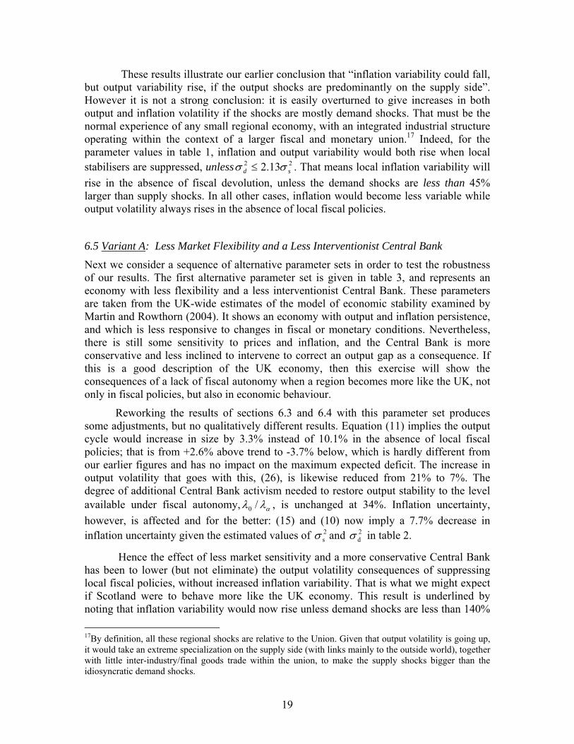
These results illustrate our earlier conclusion that “inflation variability could fall, but output variability rise, if the output shocks are predominantly on the supply side”. However it is not a strong conclusion: it is easily overturned to give increases in both output and inflation volatility if the shocks are mostly demand shocks. That must be the normal experience of any small regional economy, with an integrated industrial structure operating within the context of a larger fiscal and monetary union.17 Indeed, for the parameter values in table 1, inflation and output variability would both rise when local stabilisers are suppressed, unless 22 13.2 sd σσ ≤ . That means local inflation variability will rise in the absence of fiscal devolution, unless the demand shocks are less than 45% larger than supply shocks. In all other cases, inflation would become less variable while output volatility always rises in the absence of local fiscal policies.

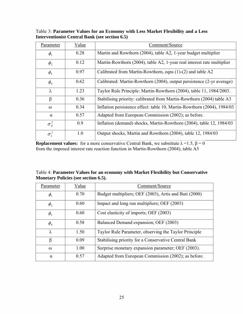
6.5 Variant A: Less Market Flexibility and a Less Interventionist Central Bank

Next we consider a sequence of alternative parameter sets in order to test the robustness of our results. The first alternative parameter set is given in table 3, and represents an economy with less flexibility and a less interventionist Central Bank. These parameters are taken from the UK-wide estimates of the model of economic stability examined by Martin and Rowthorn (2004). It shows an economy with output and inflation persistence, and which is less responsive to changes in fiscal or monetary conditions. Nevertheless, there is still some sensitivity to prices and inflation, and the Central Bank is more conservative and less inclined to intervene to correct an output gap as a consequence. If this is a good description of the UK economy, then this exercise will show the consequences of a lack of fiscal autonomy when a region becomes more like the UK, not only in fiscal policies, but also in economic behaviour.

Reworking the results of sections 6.3 and 6.4 with this parameter set produces some adjustments, but no qualitatively different results. Equation (11) implies the output cycle would increase in size by 3.3% instead of 10.1% in the absence of local fiscal policies; that is from +2.6% above trend to -3.7% below, which is hardly different from our earlier figures and has no impact on the maximum expected deficit. The increase in output volatility that goes with this, (26), is likewise reduced from 21% to 7%. The degree of additional Central Bank activism needed to restore output stability to the level available under fiscal autonomy, αλλ /0 , is unchanged at 34%. Inflation uncertainty, however, is affected and for the better: (15) and (10) now imply a 7.7% decrease in inflation uncertainty given the estimated values of 2

sσ and 2dσ in table 2.

Hence the effect of less market sensitivity and a more conservative Central Bank has been to lower (but not eliminate) the output volatility consequences of suppressing local fiscal policies, without increased inflation variability. That is what we might expect if Scotland were to behave more like the UK economy. This result is underlined by noting that inflation variability would now rise unless demand shocks are less than 140% 17By definition, all these regional shocks are relative to the Union. Given that output volatility is going up, it would take an extreme specialization on the supply side (with links mainly to the outside world), together with little inter-industry/final goods trade within the union, to make the supply shocks bigger than the idiosyncratic demand shocks.

20

larger than supply shocks ( 2s

2d 73.5 σσ ≤ ), instead of just 45% larger. The gain here is that

inflation uncertainty will be decreased over a wider range of circumstances than before. The loss is that the inflation and output cycles themselves are still larger than they would be given fiscal devolution. That means more extended periods of local unemployment or inflation; and hence larger implicit budget deficits, and surpluses forgone.

Variant B: Less Market Flexibility with Conservative Monetary Policies

What the results so far do not make clear is whether the trade off of greater output stability for increased inflation uncertainty is the result of less market flexibility, or of a more conservative Central Bank. To answer that question, we make the Central Bank more conservative in its approach to policy, and remove its tendency to intervene to remove output gaps altogether. But we retain the same market flexibility parameters as before: that is, table 3 applies with the replacement values λ=1.5 and β=0. This changes very little. Equation (11) again implies the output cycle increases 3.4% in size. Output volatility rises 6.9%, instead of 6.7%; and 0λ implies the Bank would have to be 38% more active in order to eliminate that additional volatility. Inflation volatility meanwhile would fall 7.8% (in place of 7.7%), and that will happen so long as demand shocks are less than 135% larger than supply shocks. So nothing much changes here. Evidently it is market flexibility which (perversely) creates the increased cycle and increased inflation volatility in the absence of fiscal devolution. And it is the lack of flexibility which moderates those increases, not conservatism or responsiveness at the Central Bank.

Variant C: Flexible Markets and Conservative Monetary Policies

We turn now to a third set of parameters, table 4. These values are again calibrated for the UK economy. They reflect a more market sensitive economy with a conservative but less activist Central Bank. They are taken from the UK component of the Oxford Economic Forecasting model of the world economy (OEF, 2003).

As we might expect, the combination of greater conservatism but less market inertia produces greater fluctuations in the Scottish economy in the absence of fiscal autonomy. But not greatly so. Indeed, the interesting result is to see how little the outcomes change from out first results. Equation (11) now implies that the output cycle would increase by 13.9% instead of 10%; so that national income would fluctuate between +3.5% above trend to -4.0% below, instead of from +2.5% above to -3.5 % below. As a result, the largest post 1984 deficit would have been 9.7% of GDP, and the deficit would have stood at 2.8% in 1999 on Midwinter’s figures.

For a more relevant calculation of Scotland’s position as a regional economy in the UK, these parameters imply national income would vary from 4% above the UK trend, to 4.5% below it (instead of 3.5% above to 4.0% below, as in the first example). That doesn’t change things much. The largest deficit would be 2.6% of GDP larger than that in London, and the largest surplus 2.2% larger. So once again, most of the extra instability comes out in the fiscal position. On Midwinter’s figures, the lack of fiscal

21

devolution here has cost the UK treasury additional deficits of up to an extra 1.2% of GDP (₤96m); and Scotland additional lost surpluses of 0.25% (₤18m).

Output and inflation volatility are also not much changed. Equation (26) shows that the lack of fiscal devolution will have increased output volatility by 30% instead of 21%. And in order to bring that volatility down to the level that would have prevailed with fiscal devolution, the Bank of England would have had to pursue a monetary policy that was 41% more active ( 5.1/11.2/0 =αλλ ) than permitted under this policy rule. That, as Governor Eddie George pointed out so clearly in 2001, cannot and will not happen given the monetary policy needs in the rest of the UK. Indeed, it would be inappropriate to allow it to happen when fiscal devolution at the regional level could be used to make up the difference – even though fiscal devolution would lead to an increase in inflation volatility (of 11%) at the same time, and will continue to do so unless demand shocks are less than 49% larger than supply shocks )22.2( 2

s2d σσ ≤ .

6.6 A Second Example: Fiscal Harmonisation in the European Union

A second important application of these results is the proposal for fiscal harmonisation in the Eurozone. Taken literally, this would mean removing fiscal autonomy altogether from each of the member states. Although that is a matter of removing fiscal autonomy, while the Scottish example was a case of granting fiscal autonomy, the analytic procedure is exactly the same: send local fiscal policy (α) to zero and trace out the consequences for output and inflation stability, and the size of public sector deficits/surpluses that result.

To do this for the typical Euro economy, we take the European Commission’s estimate of α = 0.5 (for the reasons discussed in section 4.3 above). The remaining parameters for our typical EU economy are set out in table 5. They are derived from the Euro area estimates of the Martin-Rowthorn model of economic stability, and calibrated in the same way as the UK-wide estimates in table 3. They depict an economy with relatively little market flexibility, much like Variant B above but with more persistence and a more aggressively anti-inflation Central Bank. We also consider a variant in which the European Central Bank does not correct output gaps at all.

Interestingly, and in contrast to the Scottish case, the results show that fiscal harmonisation would do rather little damage to the stability of the average Euro area economy. Equation (11) shows that the output cycle would increase by 1.6% in size: less than one half as much as in the Scottish case. Consequently, an economy whose cycle deviated from trend by 4% (the maximum figure likely in the EU according to the results quoted in our benchmark case; section 4.1), would now find its cycle deviating by 4.06%. And a country expected to satisfy the Stability and Growth Pact with a maximum deficit of 3% GDP, will now find that deficit expanding to 3.1%.

The results are a little stronger in terms of volatility indicators. Equation (26) implies output variability would rise 3.25%, half to one third as much as in our previous examples. This, in turn, implies the European Central Bank would have to be 14% more active in its monetary policies in order to return economic performance to its previous (no harmonisation) level. While not difficult, this is unlikely to be welcome at the ECB – if only because inflation volatility would drop by 11%, using (15) and (10). The ECB might

22

well take that as sufficient reason not to step up its interventions. Finally, the chances of having inflation volatility rise along with output instability (as opposed to having just the latter increase) are also much lower than in the UK-Scotland case. Here it will only happen if demand shocks are more than 250% larger than supply shocks on average (compared to when they are 45% larger).

A non-interventionist central bank makes no difference to these results. With the same inflation aversion (λ = 1.63), setting β = 0 produces the same output variability; a need for the ECB to increase its level of activism by 15%, and a fall in inflation volatility of 12%. Once again, central bank behaviour has very little influence on, or ability to correct, the consequences of fiscal harmonisation. That is as we found before. The difference is that fiscal harmonisation in Europe appears to make very little difference to economic stability or, by implication, to the budget deficits or surpluses that follow from that. Eliminating fiscal devolution in the UK is therefore likely to increase the cycle, and inflation and output volatility, by two to five times as much as in the EU; and to double the need for activism in monetary policy, to halve the reductions in inflation uncertainty and to increase the chances of getting higher inflation volatility along with rising output variability.

7. Conclusions 1) The advantage of suppressing local fiscal policies can only be lower inflation volatility or inflation uncertainty, and then only in an economy with limited market flexibility and where demand shocks do not dominate.

2) In general, a lack of fiscal devolution will lead to increased output and inflation cycles; and to increased output volatility (more fluctuations within those cycles); and also to extra inflation uncertainty if demand shocks are large and/or markets are flexible. Thus output fluctuations are bound to rise on either measure. The same may hold for inflation variability. But the possibility that inflation volatility can fall with an expanding cycle suggests inflation and unemployment would become more predictable, but subject to larger swings and hence longer periods away from equilibrium.

3) Evaluating these result empirically showed that increased output and inflation cycles, together with increased output volatility and more predictable (persistent) inflation in the short run, are the likely outcomes of fiscal harmonisation in the Euro area and of the lack of devolution in the UK.

4) There is an interesting difference in the empirical results here. Imposing fiscal harmonisation on the typical Euro economy would cause very little damage. Output and inflation cycles would increase by less than 2%, which means the maximum expected budget deficits would increase very little (0.1% of GDP). That would not strain the Stability Pact. Similarly, while short run output instability is bound to rise, inflation uncertainty would fall by more and the ECB would not be under pressure to intervene more actively. Hence, although such a move would be welfare reducing and represent an unstable political equilibrium, the effects would be small and could be tolerated if there were good reasons to do so.

23

In the UK, the results are different. Here both cycles increase by up to 14% in the absence of devolution, meaning an equal increase in the burden of the (implicit) regional deficit on central funding. Short term volatility also rose by more, by up to 30%, and inflation variability too depending on degree of market flexibility and the incidence of shocks. Moreover, it would require unreasonable increases in the Bank of England’s activism to counter that. Yet a government that ignores these aspects of the problem is likely to be penalised at the polls (Demertzis et al 2004). Consequently the damage done here is more substantive; and the welfare losses and unstable political equilibrium that follow, a distinct disadvantage.

5) All these numerical results appear to be robust to variations in the parameterisation of the economy, market flexibility or Central Bank behaviour.

6) The role of market flexibility is important. On the one hand, greater market flexibility can reduce swings in the budget and alleviate the strain on public finances. It may therefore help moderate the impact of increased cycles on the budget when local fiscal policies are suppressed. On the other hand, it may increase the short run volatility of inflation if the demand shocks are not small; and it certainly increases output volatility in all cases. Hence, creating less flexible markets will typically mean trading less exaggeration of the cycle and less short run volatility, for less ability to adjust around the cycle – as evidenced here by the larger fiscal deficits and surpluses, and more persistent unemployment or inflation, which appear in those cases. This may seem perverse, but it is a perfect illustration of a result that has appeared in a number of earlier papers18-- that a flexible economy, in a union with less flexible neighbours, will inevitably carry (some of) the burden of adjustment for those neighbours simply because that economy’s markets are able to provide the necessary wage-price or quantity-employment changes relatively quickly or easily. But that would mean greater short run volatility while those adjustments are made, even if the long term cycle is eventually moderated.19

18 Dellas and Tavlas (2003), Hughes Hallett and Viegi (2003), HM Treasury (2003), Hughes Hallett and Jensen (2003), Hughes Hallett et al (2004). 19 This would be a cost to the flexible economy, but a gain for the Union as a whole, if volatility were known to damage overall performance (growth, employment, inflation). Several studies have shown increasing short term volatility in the flexible economy, but lower volatility in the union or its less flexible members, when local policy instruments are restricted or withdrawn (Fair 1998, Barrell and Dury 2000). But things are less clear cut in practice. Conventional wisdom says that volatility is damaging to growth (Ramey and Ramey, 1995). However, a closer look at the data shows that volatility appears to encourage growth in the industrial and industrializing countries – in particular when it comes from trade or financial liberalization (Kose, et al, 2004). That is, when it comes from greater market flexibility. So greater volatility can be helpful as a substitute for local policy measures, which is precisely our result here. Indeed, even when there is a negative relation between growth and volatility, greater market flexibility has typically reduced that association – which is again our result.

24

Table 1: Parameter Values for a small, open market based economy with a liberal Central Bank (see section 6.3).

Parameter Value Comment/Source

1φ 0.50 After two years; TRYM (1996)

2φ 0.63 After two years; TRYM (1996)

3φ 0.77 Long run price elasticity of imports; TRYM (1996)

4φ 0.21 Domestic Absorption Parameters; TYRM (1996)

λ 0.68 Interest rate reaction function

β 1.00 Adapted from TRYM (1996)

ω 1.00 Annualised output gap model (table 2, Gruen et al 2002)

α 0.57 Adapted from European Commission (2002); see text.

All parameter values, except α, are calibrated using the TRYM model

Table 2: The Percentage Increase in the Variability of Inflation and Output when Fiscal Devolution Is Suppressed

a) Increases in Inflation Variability (%)

2sσ

2dσ

0.1

0.5

1.0

2.0

5.0

0.1 -5.06 -10.41 -11.26 -11.67 -11.95

0.5 6.97 -5.06 -8.80 -10.03 -11.25

1.0 12.13 -0.47 -5.06 -8.17 -10.43

2.0 15.92 5.14 -0.46 -5.06 -8.88

5.0 18.82 12.13 6.98 1.28 -5.06

10.0 19.93 15.92 12.14 6.97 -0.47

b) Increases in Output Variability

= 0.211 via (26),

or a 21.1% increase in variance of output independently of the shock structure.

25

Table 3: Parameter Values for an Economy with Less Market Flexibility and a Less Interventionist Central Bank (see section 6.5)

Parameter Value Comment/Source

1φ 0.28 Martin and Rowthorn (2004), table A2, 1-year budget multiplier

2φ 0.12 Martin-Rowthorn (2004), table A2, 1-year real interest rate multiplier

3φ 0.97 Calibrated from Martin-Rowthorn, eqns (1)-(2) and table A2

4φ 0.62 Calibrated: Martin-Rowthorn (2004), output persistence (2-yr average)

λ 1.23 Taylor Rule Principle: Martin-Rowthorn (2004), table 11, 1984/2003.

β 0.36 Stabilising priority: calibrated from Martin-Rowthorn (2004) table A3

ω 0.34 Inflation persistence effect: table 10, Martin-Rowthorn (2004), 1984/03

α 0.57 Adapted from European Commission (2002); as before. 2dσ 0.9 Inflation (demand) shocks, Martin-Rowthorn (2004), table 12, 1984/03

2sσ 1.0 Output shocks, Martin and Rowthorn (2004), table 12, 1984/03

Replacement values: for a more conservative Central Bank, we substitute λ =1.5, β = 0 from the imposed interest rate reaction function in Martin-Rowthorn (2004), table A5

Table 4: Parameter Values for an economy with Market Flexibility but Conservative Monetary Policies (see section 6.5).

Parameter Value Comment/Source

1φ 0.70 Budget multipliers; OEF (2003), Artis and Buti (2000)

2φ 0.60 Impact and long run multipliers; OEF (2003)

3φ 0.60 Cost elasticity of imports; OEF (2003)

4φ 0.58 Balanced Demand expansion; OEF (2003)

λ 1.50 Taylor Rule Parameter, observing the Taylor Principle

β 0.09 Stabilising priority for a Conservative Central Bank

ω 1.00 Surprise monetary expansion parameter; OEF (2003).

α 0.57 Adapted from European Commission (2002); as before.

26

Table 5: Parameter Values for a Euro Area Economy, with a Conservative Central Bank, Fiscal Harmonisation and Persistence (section 6.6)

Parameter Value Comment/Source

1φ 0.28 Martin and Rowthorn (2004), table A2, 1-year budget multiplier

2φ 0.16 Martin-Rowthorn (2004), table A2, 1-year real interest rate multiplier

3φ 1.68 Calibrated from Martin-Rowthorn(2004), eqns (1)-(2) and table A2

4φ 0.68 Calibrated: Martin-Rowthorn (2004), output persistence (2-yr average)

λ 1.63 Taylor Rule Principle: Martin-Rowthorn (2004), table 11, 1984/2003.

β 0.32 Stabilising priority: calibrated from Martin-Rowthorn (2004) table A3

ω 0.28 Inflation persistence effect: table 10, Martin-Rowthorn (2004), 1984/03

α 0.5 European Commission (2002); standard EU economy. 2dσ 0.4 Inflation (demand) shocks, Martin-Rowthorn (2004), table 12, 1984/04

2sσ 1.0 Output shocks, Martin and Rowthorn (2004), table 12, 1984/03

Replacement values: for a more conservative Central Bank, we substitute λ =1.63, β = 0 from the imposed interest rate reaction function in Martin-Rowthorn (2004), table A5

References: Akerlof G, W Dickens and G L Perry (2000), “Near-Rational Wage and Price Setting and the Long Run Philips Curve”, Brookings Papers on Economic Activity, 200:1, 1-44.

Artis M., and Marco Buti, (2000), “Close to Balance or in Surplus: A Policy Makers Guide to the Implementation of the Stability Pact”, Journal of Common Market Studies, 38, 563-91.

Ball L, “Efficient Rules for Monetary Finance”, International Finance, 2, 63-83.

Barrell R and K Dury (2000) “Choosing the Regime: Macroeconomic Effects of UK Entry”, Journal of Common Market Studies, 38, 625-44.

Bean C (1998), “The New UK Monetary Arrangements: A View from the Literature” Economic Journal, 108, 1795-1809.

Brunila Anne, Marco Buti and J. in ‘t Veld (2003) “Cyclical Stabilisation under the Stability and Growth Pact: How Effective are Automatic Stabilisers” Empirica, 31, 1-24.

Buti, Marco, Daniele Franco and H. Ongena (1998) “Fiscal Discipline and Flexibility in EMU: the Implementation of the Stability and Growth Pact” Oxford Review of Economic Policy, 14 (3), 81-97.

27

Coenen G and V Wieland (2002), “Inflation Dynamics and International Linkages:A Model of the United States, Euro area and Japan”., ECB Working Paper 181, ECB, Frankfurt.

Cuthbert M (2003) “Scotland Devolved and Monetary Union” Scottish Affairs, 45, 20-43.

Dellas H and G Tavlas (2003),“Wage Rigidity and Monetary Union” Economic Journal (forthcoming).

Demertzis M, A Hughes Hallett and N Viegi (2004) “An Independent Central Bank Faced with Elected Governments”, European Journal of Political Economy, 20, 907-22.

European Commission (2002) “Public Finances in EMU: 2” The European Economy; Reports and Studies 4, European Commission, Brussels.

Fair R (1998), “Estimated Stabilisation Costs of EMU”, National Institute Economic Review, 98, 90-99.

Gruen D, T Robertson and Andrew Stone (2002) “Output Gaps in Real Time: Are they reliable enough to use for monetary policy?” Working Paper 2002-06, Reserve Bank of Australia, Sydney.

HM Treasury (2003) “Modelling Shocks and Adjustment Mechanisms in EMU”, in UK Membership of the Single Currency: An Assessment of the Five Economic Tests, HMSO, London, Command 5776.

Hughes Hallett A and S E H Jensen (2003) “Labour Market reform and the Enlargement of a Monetary Union”, CESifo Economic Studies, 49, 355-79.

Hughes Hallett A and N Viegi (2003) “Labour Market Reform and the Effectiveness of Monetary Policy in EMU”, Journal of Economic Integration, 18, 726-49.

Hughes Hallett A, S E H Jensen and C Richter (2004) “The European Economy at the Cross Roads: Structural Reforms, Fiscal Constraints and the Lisbon Agenda”, Research in International Business and Finance, (forthcoming).

Kose M, E Prasad and M Terrones “How Do Trade and Financial Integration Affect the Relationship between Growth and Volatility?”, Working Paper, IMF (forthcoming).

Martin B and R Rowthorn (2004),“Will Stability Last?”, Faculty of Economics, Uni-versity of Cambridge, (7 September, 2004).

Midwinter A (2001) “Unworkable in Practice: A Critique of Fiscal Autonomy”, in Jamieson W (ed) “Calling Scotland to Account”, The Policy Institute, Edinburgh.

Mood A, F Graybill and D Boes (1974), “Introduction to the Theory of Statistics”, third edition, McGraw-Hill, New York.

OEF (2003), “The New OEF Windows World Model Software”, Oxford Economic Forecasting, Oxford, UK.

RBA (2002) “The Effects of Growth on the Budget Balance: a Rule of Thumb” Economic Analysis Department, Reserve Bank of Australia, Sydney, 25th January 2002.

Ramey G and V Ramey (1995), “Cross-Country Evidence on the Link between Volatility and Growth”, American Economic Review, 85, 1138-51.

28

Rudebusch G and L Svensson (1999), “Policy Rules for Inflation Targeting” in J B Taylor (ed), Monetary Policy Rules, University of Chicago Press, Chicago.

Svennson L (1997), “Inflation Forecast Targeting: Implementing and Monitoring Inflation Targets”, European Economic Review, 41, 1111-46.

TRYM (1996) “The Macroeconomics of the TRYM Model of the Australian Economy” Macroeconomics Analysis Branch, Commonwealth Treasury, Canberra. (www.treasury.gov.au/documents/238/PDF/trym_m.pdf)