EDDY CURRENT METHODOLOGIES FOR RELIABLE DETECTION AND RAPID IMAGING OF SUB-SURFACE FLAWS

IN STAINLESS STEEL

By

ANIL KUMAR SONI (Enrollment No: ENGG02201104009)

Indira Gandhi Centre for Atomic Research, Kalpakkam

A thesis submitted to the Board of Studies in Engineering Sciences

In partial fulfillment of requirements for the Degree of

DOCTOR OF PHILOSOPHY

of

HOMI BHABHA NATIONAL INSTITUTE

August, 2016

STATEMENT BY GUIDE

I hereby certify that I have read this dissertation prepared under my direction and recommend that it

may be accepted as fulfilling the dissertation requirement.

Date: 05/08/2016 (Dr. B. Purna Chandra Rao)

Place: Kalpakkam Guide / Convener

STATEMENT BY AUTHOR

This dissertation has been submitted in partial fulfillment of requirements for an advanced degree at

Homi Bhabha National Institute (HBNI) and is deposited in the library to be made available to

borrowers under rules of the HBNI.

Brief quotations from this dissertation are allowable without special permission, provided that accurate

acknowledgement of source is made. Requests for permission for extended quotation from or

reproduction of this manuscript in whole or in part may be granted by the Competent Authority of

HBNI when in his or her judgment the proposed use of the material is in the interests of scholarship. In

all other instances, however, permission must be obtained from the author.

Date : 05/08/2016

Place : Kalpakkam (Anil Kumar Soni)

DECLARATION

I, hereby declare that the investigation presented in the thesis entitled “Eddy current methodologies

for reliable detection and rapid imaging of sub-surface flaws in stainless steel” submitted to Homi

Bhabha National Institute (HBNI), Mumbai, India, for the award of Doctor of Philosophy in

Engineering Sciences, is the record of work carried out by me under the guidance of

Dr. B. Purna Chandra Rao, Head, Non­Destructive Evaluation Division, Metallurgy and Materials

Group, Indira Gandhi Centre for Atomic Research, Kalpakkam. The work is original and has not been

submitted earlier as a whole or in part for a degree / diploma at this or any other Institution/University.

Date : 05/08/2016

Place : Kalpakkam (Anil Kumar Soni)

LIST OF PUBLICATIONS ARISING FROM THE THESIS

JOURNALS

1. Anil Kumar Soni, S. Thirunavukkarasu and B. Purna Chandra Rao, ‘Bayes principle based multi­

resolution wavelet transform image processing method for enhancement of sub­surface defect

images ’, Sensor Review (Under preparation).

2. Anil Kumar. Soni, B. Purna Chandra Rao, S. Mahadevan and S. Thirunavukkarasu, ‘A study on

the scan plans for rapid eddy current non­destructive evaluation’, Journal of Nondestructive

Evaluation (Under Review).

3. Anil Kumar Soni, B. Sasi, S. Thirunavukkarasu and B. Purna Chandra Rao ‘Development of

eddy current probe for detection of deep sub­surface defects’, IETE Technical Review,

November 2015, DOI: 10.1080/02564602.2015.1113145.

4. Anil Kumar. Soni, S. Thirunavukkarasu, B. Sasi, B. Purna Chandra Rao, T. Jayakumar,

‘Development of a high sensitive eddy current instrument for detection of sub­surface defects in

stainless steel plates’, Insight­Non­Destructive Testing & Condition Monitoring Vol. 57, No. 9,

September 2015, pp. 508­512, DOI: 10.1784/insi.2015.57.9.508.

5. S. Thirunavukkarasu, B. Purna Chandra Rao, Anil Kumar Soni, S. Shuaib Ahmed, T. Jayakumar,

‘Comparative performance of image fusion methodologies in eddy current testing’, Research

Journal of Applied Sciences, Engineering and Technology, Vol. 4, No. 24, 2012, pp. 5548­5551.

CONFERENCES

1. Anil Kumar Soni, S Shuaib Ahmed, S. Thirunavukkarasu, B. Purna Chandra Rao and T

Jayakumar, ‘Multi­Sensor Image Fusion for Enhanced Detection of Sub­Surface Defects by Eddy

Current Testing’, Presented during the 14th Asia Pacific Conference on Non­destructive Testing,

Mumbai, 2013.

2. Anil Kumar Soni, B. Purna Chandra Rao, B. Sasi, Saji Jacob George, T Jayakumar,

‘Development of a Low Frequency Eddy Current Instrument for Non­destructive Evaluation’,

Presented during the National Symposium on Instrumentation (NSI­38), Hubli, 2013.

OTHERS

1. C.S. Angani, Anil Kumar Soni, K. Sambasiva Rao, Jaskaran Singh Grover, S. Thirunavukkarasu,

B. Purna Chandra Rao, T. Jayakumar, ‘Development of Pulsed Eddy Current System and Model

Based Optimization’, Presented during the National Seminar on NDE­2012, New Delhi, 2012.

(Anil Kumar Soni)

DEDICATED TO MY BELOVED

PARENTS

ACKNOWLEDGEMENTS

This thesis would not have been possible without the support and encouragement of many people who

contributed and extended their valuable co­operation in the completion of the research work. I feel

short of words in expressing my appreciation for their help at various stages of this work.

First and foremost, I would like to express my sincere gratitude to my thesis advisor Dr. B. Purna

Chandra Rao Head, Non­destructive Evaluation Division (NDED), Indira Gandhi Centre for Atomic

Research (IGCAR) for his continuous support to my work, his patience, encouragement, enthusiasm

and immense knowledge. His intellectual ideas and guidance helped me in my research work and

writing this thesis. He has always been a source of motivation for me in difficult times in research or

otherwise. I express my deep sense of appreciation for his support and for energizing me to overcome

all the hurdles. I take this opportunity to thank my Co­Guide Dr. B. K. Panigrahi for regular appraisal,

kind advice and suggestions to improve the quality of my work.

I thank my doctoral committee; Chairman Dr. K. Velusamy and member Dr. M. Sai Baba for their

encouragement, insightful comments and fruitful ideas during the course of the thesis work which

have been useful for the progress of my work. I express my sincere gratitude to Dr. T. Jayakumar,

former Director, Metallurgy and Materials Group (MMG), IGCAR for the inspiration and

encouragement. I extend my heartfelt thanks to the former directors of IGCAR, Shri S. C. Chetal and

Dr. P. R. Vasudeva Rao and to the present Director, Dr. S.A.V. Satya Murty for permitting me to

pursue research in this reputed centre. I wish to acknowledge Dr. C. K. Mukhopadhyay, Head EMSI

Section, NDED, IGCAR, for providing his valuable suggestions at various occasions.

I express my gratitude to Dr. S. Thirunavukkarasu, Smt B. Sasi, and Shri S. Mahadevan, NDED,

IGCAR for helping me in learning the instrumentation and experimental techniques and providing me

technical support and guidance during the entire research work. I share the credit of my work with

them for helping me in carrying out the experiments round the clock and enriching my ideas.

I thank my lab mates Dr. G. K. Sharma, Dr. C. S. Angani, Dr. W. Sharatchandra Singh, Shri S.

Ponseenivasan, Shri V. Arjun, Shri K. Samba Siva Rao, Dr. S. Shuaib Ahmed, Shri K. Arunmuthu,

Shri A. Viswanath and other NDED staff members for their timely help, useful technical discussions,

suggestions, and moral support.

Apart from the intellectual support, an emotional support is always needed to conquer the hardships.

For this, I would like to thank, from the bottom of my heart, my friends Ashutosh Mishra, M. Kalyan

Phani, B. Rakesh, K. Siva Srinivas, Chandan Kumar Bhagat, B. K. Srihari, Deepak CH., Arun Babu,

Paawan Sharma, M. Bubathi, Sharath D, M. S. K. Chaitanya, G.V.K. Kishore and S. Naveen for their

warm friendship.

Last but not the least, my deepest gratitude is to my family for their warm support which brings belief

and hope into my life; to my beloved parents Shri Ram Kumar Soni and Smt. Krishna Soni, who have

been so caring and supportive of me all the time; to my wife Smt Aradhana Soni, who has been

always with me as my strength for up and down moments during my research work; and my

grandparents, who have always been a source of inspiration towards achieving the goals in life.

Immense love and affection of my sister Radhika Soni and brother Vikas Soni have been invaluable

in the journey towards my goal.

Apart from all the people mentioned in this acknowledgment, there are many others who have helped

me in various ways during the course of this thesis work. My sincere thanks and apologies to all those

I may have forgotten to mention.

(Anil Kumar Soni)

i

TABLE OF CONTENTS TABLE OF CONTENTS . . . . . . . . . . . . . . . . . . . . . . . . . . . . . . . . . . . . . . . . . . . . . . . . . . . . . . . . . . . . . . . . . . . i

Abstract . . . . . . . . . . . . . . . . . . . . . . . . . . . . . . . . . . . . . . . . . . . . . . . . . . . . . . . . . . . . . . . . . . . . . . . . . . . . . . . . . . . . . . . . . v

List of Fig ures . . . . . . . . . . . . . . . . . . . . . . . . . . . . . . . . . . . . . . . . . . . . . . . . . . . . . . . . . . . . . . . . . . . . . . . . . . . . . . vi i

List of Tab les . . . . . . . . . . . . . . . . . . . . . . . . . . . . . . . . . . . . . . . . . . . . . . . . . . . . . . . . . . . . . . . . . . . . . . . . . . . . . . . x i i i

Nomenclature . . . . . . . . . . . . . . . . . . . . . . . . . . . . . . . . . . . . . . . . . . . . . . . . . . . . . . . . . . . . . . . . . . . . . . . . . . . . . . . . xv

1 Introduction . . . . . . . . . . . . . . . . . . . . . . . . . . . . . . . . . . . . . . . . . . . . . . . . . . . . . . . . . . . . . . . . . . . . . . . . . . . . . . 1

1. 1 NON­DESTRUCTIVE EVALUATION . . . . . . . . . . . . . . . . . . . . . . . . . . . . . . . . . . . . . . . . . . . . . . . . . . . . . . 1

1. 2 EDDY CURRENT TESTING . . . . . . . . . . . . . . . . . . . . . . . . . . . . . . . . . . . . . . . . . . . . . . . . . . . . . . . . . . . . . . . . . . 5

1.2.1 Principle of eddy current testing ............................................................................................. 5

1.2.2 Detection of surface flaws ...................................................................................................... 8

1.2.3 Detection of sub­surface flaws ...............................................................................................12

1. 3 CONSIDARATIONS FOR DETECTION OF SUB­SURF ACE FLAWS . . . . . . . . . . . . 12

1.3.1 Excitation frequency ..............................................................................................................13

1.3.2 Electromagnetic coupling ......................................................................................................14

1.3.3 Eddy current probe ................................................................................................................14

1.3.4 Excitation field strength .........................................................................................................16

1.3.5 Reception unit .......................................................................................................................17

1.3.6 Processing of Signals and images...........................................................................................18

1.3.7 Fusion of images ...................................................................................................................18

1. 4 LITE RATURE REVIEW . . . . . . . . . . . . . . . . . . . . . . . . . . . . . . . . . . . . . . . . . . . . . . . . . . . . . . . . . . . . . . . . . . . . . . 24

1.4.1 Eddy current probe ................................................................................................................24

1.4.2 Eddy current instrumentation .................................................................................................29

1.4.3 Signal and image processing ..................................................................................................32

1.4.4 Rapid detection and imaging ..................................................................................................34

1. 5 SUMMARY . . . . . . . . . . . . . . . . . . . . . . . . . . . . . . . . . . . . . . . . . . . . . . . . . . . . . . . . . . . . . . . . . . . . . . . . . . . . . . . . . . . . . . 39

2 Motivat ion and Object ive . . . . . . . . . . . . . . . . . . . . . . . . . . . . . . . . . . . . . . . . . . . . . . . . . . . . . . . . . 41

ii

2. 1 PREAMBLE . . . . . . . . . . . . . . . . . . . . . . . . . . . . . . . . . . . . . . . . . . . . . . . . . . . . . . . . . . . . . . . . . . . . . . . . . . . . . . . . . . . . . . 41

2. 2 MOTIVATION FOR RE SEARCH . . . . . . . . . . . . . . . . . . . . . . . . . . . . . . . . . . . . . . . . . . . . . . . . . . . . . . . . . . . 41

2. 3 OBJECTIVE OF RESEARCH . . . . . . . . . . . . . . . . . . . . . . . . . . . . . . . . . . . . . . . . . . . . . . . . . . . . . . . . . . . . . . . . 43

2. 4 ORGANIZATION OF THE THES IS . . . . . . . . . . . . . . . . . . . . . . . . . . . . . . . . . . . . . . . . . . . . . . . . . . . . . . . . 44

3 Design and development of eddy current probe . . . . . . . . . . . . . . . . . . . . . . . . . . . 46

3. 1 PREAMBLE . . . . . . . . . . . . . . . . . . . . . . . . . . . . . . . . . . . . . . . . . . . . . . . . . . . . . . . . . . . . . . . . . . . . . . . . . . . . . . . . . . . . . . 46

3. 2 FIN ITE ELE MENT MODELLING . . . . . . . . . . . . . . . . . . . . . . . . . . . . . . . . . . . . . . . . . . . . . . . . . . . . . . . . . . 46

3. 3 GOVER NING EQUATIONS FOR EDDY CURRENT TESTING. . . . . . . . . . . . . . . . . . . . . 47

3. 4 FIN ITE ELE MENT MODEL FOR EDDY CURRENT TESTING . . . . . . . . . . . . . . . . . . . . 48

3.4.1 Construction of model geometry ............................................................................................ 48

3.4.2 Meshing ................................................................................................................................ 50

3.4.3 Equation solving ................................................................................................................... 50

3.4.4 Post­processing ..................................................................................................................... 51

3. 5 MODEL BASED OPTIM ISA TION OF PROBE CONFIGURATION . . . . . . . . . . . . . . . . 51

3. 6 RESULTS AND DISCUSSION . . . . . . . . . . . . . . . . . . . . . . . . . . . . . . . . . . . . . . . . . . . . . . . . . . . . . . . . . . . . . . 54

3.6.1 Model predicted magnetic field and flux density .................................................................... 54

3.6.2 Model predicted eddy current density .................................................................................... 55

3.6.3 Model predicted change in phase angle (∆θ) .......................................................................... 58

3.6.4 Optimisation of outer diameter of cup­core probe configuration ............................................. 60

3.6.5 Selection of excitation frequency of cup­core probe ............................................................... 62

3. 7 EXPERIMENTAL STUDIE S USING OPTIMISED CUP ­CORE PROBE . . . . . . . . . . 64

3. 8 SUMMARY . . . . . . . . . . . . . . . . . . . . . . . . . . . . . . . . . . . . . . . . . . . . . . . . . . . . . . . . . . . . . . . . . . . . . . . . . . . . . . . . . . . . . . . 65

4 Development o f high sensi t ive eddy current instrument . . . . . . . . . . . . . . . 67

4. 1 PREAMBLE . . . . . . . . . . . . . . . . . . . . . . . . . . . . . . . . . . . . . . . . . . . . . . . . . . . . . . . . . . . . . . . . . . . . . . . . . . . . . . . . . . . . . . 67

4. 2 DESIGN OF EDDY CURRENT INSTRUMENT . . . . . . . . . . . . . . . . . . . . . . . . . . . . . . . . . . . . . . . . . 67

4.2.1 Excitation unit ....................................................................................................................... 69

4.2.2 Reception unit ....................................................................................................................... 71

4.2.3 Data acquisition and probe scanning ...................................................................................... 73

4. 3 TEST SPECIMENS F OR EXPERIMENTS . . . . . . . . . . . . . . . . . . . . . . . . . . . . . . . . . . . . . . . . . . . . . . . . 76

4. 4 PERFORMANCE ASS ESS MENT OF EDDY CURRENT INS TRUMENT . . . . . . . . . 78

iii

4.4.1 Influence of excitation current ...............................................................................................78

4.4.2 Phase angle resolution ...........................................................................................................80

4.4.3 Drift ......................................................................................................................................81

4.4.4 Response of eddy current instrument......................................................................................82

4. 5 RES ULTS AND DISCUS SION . . . . . . . . . . . . . . . . . . . . . . . . . . . . . . . . . . . . . . . . . . . . . . . . . . . . . . . . . . . . . 85

4.5.1 Sub­surface flat bottom holes.................................................................................................86

4.5.2 Sub­surface notches ...............................................................................................................86

4.5.3 Surface flaws.........................................................................................................................87

4. 6 IMAGING OF S UB­SURFACE FLAWS . . . . . . . . . . . . . . . . . . . . . . . . . . . . . . . . . . . . . . . . . . . . . . . . . . 89

4. 7 SUMMARY . . . . . . . . . . . . . . . . . . . . . . . . . . . . . . . . . . . . . . . . . . . . . . . . . . . . . . . . . . . . . . . . . . . . . . . . . . . . . . . . . . . . . . 90

5 Development o f image fusion methodology . . . . . . . . . . . . . . . . . . . . . . . . . . . . . . . . . 91

5. 1 PRE AMBLE . . . . . . . . . . . . . . . . . . . . . . . . . . . . . . . . . . . . . . . . . . . . . . . . . . . . . . . . . . . . . . . . . . . . . . . . . . . . . . . . . . . . . 91

5. 2 IMAGE FUSION . . . . . . . . . . . . . . . . . . . . . . . . . . . . . . . . . . . . . . . . . . . . . . . . . . . . . . . . . . . . . . . . . . . . . . . . . . . . . . . 91

5. 3 PROPOSED BAYWT BASED IMAGE FUSION METHODOLOGY . . . . . . . . . . . . . . . . 92

5. 4 INPU T EDDY CURRENT IMAGES . . . . . . . . . . . . . . . . . . . . . . . . . . . . . . . . . . . . . . . . . . . . . . . . . . . . . . . 94

5. 5 PERFORMANCE EVALUATION OF BAYWT IMAGE FUS ION. . . . . . . . . . . . . . . . . . . 94

5.5.1 Standard deviation .................................................................................................................95

5.5.2 Entropy .................................................................................................................................95

5.5.3 Signal­to­noise ratio ..............................................................................................................96

5.5.4 Fusion mutual information .....................................................................................................96

5.5.5 Results and discussion ...........................................................................................................97

5. 6 COMP ARISON OF PERF ORMANCE OF DIFF ERENT FUS ION

METHODOLOGIE S . . . . . . . . . . . . . . . . . . . . . . . . . . . . . . . . . . . . . . . . . . . . . . . . . . . . . . . . . . . . . . . . . . . . . . . 100

5. 7 SUMMARY . . . . . . . . . . . . . . . . . . . . . . . . . . . . . . . . . . . . . . . . . . . . . . . . . . . . . . . . . . . . . . . . . . . . . . . . . . . . . . . . . . . . . 102

6 Novel scan methodology for rapid detect ion and imag ing of f laws105

6. 1 PRE AMBLE . . . . . . . . . . . . . . . . . . . . . . . . . . . . . . . . . . . . . . . . . . . . . . . . . . . . . . . . . . . . . . . . . . . . . . . . . . . . . . . . . . . . 105

6. 2 PARAMETERS FOR RAP ID SCAN PLANS . . . . . . . . . . . . . . . . . . . . . . . . . . . . . . . . . . . . . . . . . . . . 105

6. 3 DESCRIPTION OF THE SCAN PLANS . . . . . . . . . . . . . . . . . . . . . . . . . . . . . . . . . . . . . . . . . . . . . . . . . 106

6.3.1 Raster scan .......................................................................................................................... 106

6.3.2 Diagonal raster scan ............................................................................................................ 107

iv

6.3.3 Spiral scan .......................................................................................................................... 107

6.3.4 Lissajous scan ..................................................................................................................... 109

6.3.5 Billiard scan ........................................................................................................................ 109

6. 4 IMP LEMENTATION OF SCAN PLANS . . . . . . . . . . . . . . . . . . . . . . . . . . . . . . . . . . . . . . . . . . . . . . . . 111

6.4.1 Numerical investigations ..................................................................................................... 111

6.4.2 Experimental verification .................................................................................................... 112

6. 5 AS SES SMENT OF RAP ID S CAN PLANS . . . . . . . . . . . . . . . . . . . . . . . . . . . . . . . . . . . . . . . . . . . . . . 114

6.5.1 Rapid detection of a flaw .................................................................................................... 114

6.5.2 Complete coverage of scanning area .................................................................................... 117

6.5.3 Step size for detection of flaw.............................................................................................. 120

6. 6 BILLIARD SCAN PLAN . . . . . . . . . . . . . . . . . . . . . . . . . . . . . . . . . . . . . . . . . . . . . . . . . . . . . . . . . . . . . . . . . . . . 122

6.6.1 Influence of notch location .................................................................................................. 122

6.6.2 Influence of notch dimensions ............................................................................................. 122

6.6.3 Influence of angle of incidence ............................................................................................ 123

6.6.4 Step size for the billiard scan plan........................................................................................ 124

6. 7 EXPERIMENTAL VERIF ICATION OF THE BILLIARD SCAN PLAN . . . . . . . . . 126

6. 8 SUMMARY . . . . . . . . . . . . . . . . . . . . . . . . . . . . . . . . . . . . . . . . . . . . . . . . . . . . . . . . . . . . . . . . . . . . . . . . . . . . . . . . . . . . . 128

7 Conclusion a nd Future wo rks . . . . . . . . . . . . . . . . . . . . . . . . . . . . . . . . . . . . . . . . . . . . . . . . . . 130

7. 1 CONCLUSION . . . . . . . . . . . . . . . . . . . . . . . . . . . . . . . . . . . . . . . . . . . . . . . . . . . . . . . . . . . . . . . . . . . . . . . . . . . . . . . . 130

7.1.1 Technical and scientific contributions .................................................................................. 132

7. 2 FUTURE WORKS . . . . . . . . . . . . . . . . . . . . . . . . . . . . . . . . . . . . . . . . . . . . . . . . . . . . . . . . . . . . . . . . . . . . . . . . . . . . 133

R e f e r e n c e s . . . . . . . . . . . . . . . . . . . . . . . . . . . . . . . . . . . . . . . . . . . . . . . . . . . . . . . . . . . . . . . . . . . . . . . . . . . . . . . . . 136

A p p en d i x A: The me a su r e men t f un ct io n a l g o r i t h m . . . . . . . . . . . . . . . . . . . . . 143

v

ABSTRACT

The conventional eddy current testing is confined to detection of sub­surface flaws within a depth of

5.0 mm in an austenitic stainless steel plate due to the skin­effect phenomenon. Many engineering

components are made by austenitic thick stainless steel plates in the range of 8.0 mm to 12.0 mm,

such as storage tanks. Due to the presence of hostile corrosive environment, the steel undergoes

uniform corrosion, localized pitting and stress corrosion cracking on the inner surface. Inspection of

the component surface for corrosion is essential to ensure the structural integrity of the storage tanks.

Due to the radiation environment, inspection from inner surface is not possible and detection of

inside (deep sub­surface) flaws from outer surface is a challenging application of eddy current

testing. Further, rapid automated flaw detection is essential in nuclear industry for ensuring high

probability of detection as well as minimal dose of radiation for the inspection personnel. Hence, for

reliable detection and rapid imaging of sub­surface flaws in austenitic stainless steel components,

development of effective eddy current methodologies is required.

This thesis focuses on the design and development of high throughput probes which enable higher

strength of the primary magnetic field for deeper penetration of eddy currents into the steel. Finite

element modelling based comparative studies have been carried out using COMSOL multi­physics

software for selection of optimum coil probe configuration among the send­receive type air core,

ferrite core, ferrite core with outer shielding and cup­core probes. This thesis also involves

development of a high sensitive eddy current instrument for reliable detection of deep sub­surface

flaws. The excitation unit is specially designed to drive a higher excitation current upto 1A into the

probe coil and digital lock­in amplifier is designed and implemented using LabVIEW software for

precisely measuring the phase lag of the sinusoid from flaws.

vi

To further enhance the detectability of sub­surface flaws with higher signal to noise ratio, this thesis

proposes a novel BayWT based image fusion methodology that combines the wavelet transform and

Bayesian methodologies. Performance of the proposed fusion methodology is compared with the

widely used image fusion methodologies e.g. Laplacian pyramid, wavelet transform, principal

component and Bayesian based image fusion. This thesis also proposes a novel scan plan for rapid

detection and imaging of flaws which is essential for radioactive environment. For development of

the novel scan plan, detailed systematic studies have been carried out for different scan plans viz.

raster, diagonal raster, spiral, Lissajous and billiard scan plans.

These developed methodologies are applied to 12.0 mm thick AISI type 304L stainless steel plates

for detection of flat bottom holes (simulating sub­surface localized corrosion) and EDM notches

(simulating sub­surface cracks). The methodologies presented in this thesis demonstrate the

synergistic combination of cup­core coil probe and high sensitive instrument for detection of flaws

located 8.0 mm below the surface and imaging of flaws using the novel BayWT based image fusion

methodology. This study establishes, for the first time, that the billiard scan plan is an attractive scan

plan for rapid and reliable eddy current imaging of flaws in large surfaces of electrically conducting

materials.

vii

LIST OF FIGURES

Figure 1.1: A generic non­destructive evaluation system. ............................................................ 3

Figure 1.2: Basic principle of the ECT technique......................................................................... 6

Figure 1.3: Applications of the ECT technique. ........................................................................... 9

Figure 1.4: (a) Cross section of test plate with four surface flaws of different length (b)

test plate with a flaw for EC imaging. ....................................................................... 9

Figure 1.5: Typical EC signals for four surface flaws in (a) time­domain signal

(b) impedance­plane signal. .................................................................................... 10

Figure 1.6: Typical raster scan EC images of a flaw (a) real, (b) imaginary, (c) amplitude

and (d) phase angle. ................................................................................................ 11

Figure 1.7: Standard depth of penetration and effective depth of penetration. ............................ 13

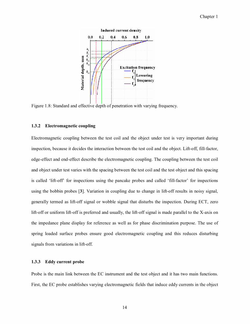
Figure 1.8: Standard and effective depth of penetration with varying frequency. ....................... 14

Figure 1.9: The typical EC probes used in various applications (a) surface (b) pencil (c)

encircling and (d) bobbin. ....................................................................................... 15

Figure 1.10: Mode of operation of EC probes (a) absolute (b) send­receive (c)

differential (d) magnetic sensor. .............................................................................. 16

Figure 1.11: Effective depth of penetration for varying excitation current. ................................. 17

Figure 1.12: Schematic diagram of Laplacian transform based image fusion. ............................ 20

Figure 1.13: Schematic diagram of wavelet transform based image fusion................................. 21

Figure 1.14: Schematic diagram for image fusion using principal component analysis. ............. 23

Figure 1.15: Cross section of surface probe over a conducting surface (a) small diameter

single coil (b) large diameter single coil and (c) double coil probe [40]. .................. 25

Figure 1.16: Predicted change rates of impedance and induced voltage due to (a) lift off

change (b) flat bottom hole depth change [40]. ........................................................ 25

Figure 1.17: Response of integrated EC GMR sensor and pancake type absolute EC

sensor signal from (a) EDM notches (b) the sensor output for flat bottom

hole located at different depths [42]. ....................................................................... 27

viii

Figure 1.18: Differential Hall sensor probe response for sample having EDM notches at

different depths [43]................................................................................................ 27

Figure 1.19: The architecture of the developed system A [53]. .................................................. 29

Figure 1.20: Signature EC signals obtained by the system A for a flaw at three excitation

frequencies [53]. ..................................................................................................... 30

Figure 1.21: (a) Schematic of I/Q detection scheme. EC images obtained using (b) the

I/Q scheme (c) traditional sample­stop­sample scheme [55]. ................................... 31

Figure 1.22: (a) Array probe with 32 absolute coils and (b) array probe 64 send­receive

mode coils. ............................................................................................................. 37

Figure 1.23: The intelligent eddy current imaging scheme developed for quick and

automated detection and characterization of flaws [82]. .......................................... 39

Figure 1.24: Three dimension image obtained by the intelligent imaging for a stainless

steel plate consisting of a notch (length 3.0 mm, width 0.3 mm and depth 0.8

mm) and a flat bottom hole (diameter 1.5 mm and depth 0.5 mm) [82]. .................. 39

Figure 3.1: The typical geometry of model with a boundary region. .......................................... 49

Figure 3.2: Discritisation of triangular mesh in the modelled geometry. .................................... 50

Figure 3.3: Typical surface and contour plot of magnetic flux density and induced

current density. ....................................................................................................... 51

Figure 3.4: Cross­section of send­receive probe configurations studied through FE

model (a) air core (b) ferrite core (c) ferrite core with outer shielding (d)

cup­core. ................................................................................................................. 52

Figure 3.5: Specimen with surface and sub­surface flaw of same depth d in 12.0 mm

thick austenitic stainless steel plate. ........................................................................ 53

Figure 3.6: Surface log plot of magnetic flux density and arrow plot of the magnetic

field for send­receive type (a) air core, (b) ferrite core, (c) ferrite core with

outer shielding and (d) cup­core eddy current probes. ............................................. 55

Figure 3.7: Surface plot of eddy current density for a sub­surface flaw located at 8.0 mm

below the surface for (a) air core, (b) ferrite core, (c) ferrite core with outer

shielding and (d) cup­core eddy current probes. ...................................................... 57

ix

Figure 3.8: Model predicted eddy current density for sub­surface flaws located at

different depths (D) below the surface for all the four type of probes. ..................... 58

Figure 3.9: Model predicted eddy current density for surface flaws of varying depths (d

= 5.0, 6.0, 7.0 and 8.0 mm) for all the four type of probes. ...................................... 59

Figure 3.10: The normalised change in phase angle (∆θ) for sub­surface flaws located at

different depths (D) below the surface. .................................................................... 59

Figure 3.11: The normalised change in phase angle (∆θ) for surface flaws of varying

depths (d = 5.0, 6.0, 7.0 and 8.0 mm). ..................................................................... 60

Figure 3.12: Model predicted normalised change in phase angle (Δθ) of the cup­core

probe at 5 kHz for various outer diameters for flaw located at 8 mm below

the surface. .............................................................................................................. 61

Figure 3.13: Model predicted induced voltage of the cup­core probe at 5 kHz for various

outer diameters for flaw located at 8 mm below the surface. .................................... 61

Figure 3.14: Model predicted eddy current density for (a) sub­surface flaw (b) surface

flaw and the normalised change in phase angle (∆θ) for (c) sub­surface flaw

(d) surface flaw of 22.0 mm diameter probes. .......................................................... 63

Figure 3.15: FE model predicted induced current density at different depth below the

surface at frequency 3 kHz, 5 kHz and 7 kHz for the 22.0 mm diameter cup­

core probe. .............................................................................................................. 64

Figure 3.16: (a) Cross section of the cup­core probe and (b) photograph of the fabricated

ECT probe. ............................................................................................................. 65

Figure 4.1: Main modules of an eddy current instrument. .......................................................... 67

Figure 4.2: Schematic block diagram of the ECT Instrument. .................................................... 69

Figure 4.3: Circuit diagram of developed excitation unit. .......................................................... 70

Figure 4.4: Schematic diagram of implementation of lock­in amplifier in LABVIEW

development environment. ...................................................................................... 73

Figure 4.5: Block diagram of the lock­in amplifier based phase measurement. .......................... 74

Figure 4.6: Front panel GUI of the lock­in amplifier based phase measurement. ........................ 75

x

Figure 4.7: Schematic of stainless steel plates with machined (a) flat bottom holes (b)

notches (width 2.5 mm) and (c) notches (width 1.0 mm). ........................................ 77

Figure 4.8: Photograph of the developed ECT instrument.......................................................... 78

Figure 4.9: Measured coil temperature as function of the excitation current in ECT

probe. ..................................................................................................................... 79

Figure 4.10: (a) Magnitude (b) change in phase angle response of the cup­core probe at

different excitation currents for sub­surface notches D3 and D4. ............................. 80

Figure 4.11: (a) Temperature of the excitation coil and (b) change in phase angle as

function of time. ..................................................................................................... 81

Figure 4.12: Time domain (a) in­phase and (b) quadrature components signals obtained

for sub­surface notches. .......................................................................................... 82

Figure 4.13: Impedance plane signals obtained for sub­surface notches. .................................... 83

Figure 4.14: (a) Peak magnitude and (b) peak of change in phase angle of sub­surface

notches. .................................................................................................................. 84

Figure 4.15: Linear behavior of notch location below the surface (D) as function of

change in phase angle (Δθ). .................................................................................... 84

Figure 4.16: Comparison of detection performance of the proposed EC instrument with

a commercial instrument. ........................................................................................ 85

Figure 4.17: EC signal obtained for 3.0 mm diameter FBHs located at different depths

(D) below the surface in a 12.0 mm thick SS plate. ................................................. 86

Figure 4.18: The EC signal obtained for sub­surface notches located at different depths

(D) below the surface. ............................................................................................. 87

Figure 4.19: The EC signal is obtained for surface notches of varying depths (d = 4.0,

6.0 and 8.0 mm) notches. ........................................................................................ 88

Figure 4.20: EC image of 4 sub­surface notches in SS plate (a) change in phase angle

(b) magnitude. ........................................................................................................ 89

Figure 5.1: Block diagram of the proposed BayWT based image fusion methodology. .............. 93

xi

Figure 5.2: CIVA model predicted phase angle images of a sub­surface flaw located at

8.0 mm below the surface at frequency (a) 5 kHz and (b) 7 kHz with

additive noise of 30% of maximum phase and SNR of 5 dB. ................................... 97

Figure 5.3: Experimentally obtained phase angle images of a sub­surface notch located

at 8.0 mm below the surface at frequency (a) 5 kHz and (b) 7 kHz. ......................... 98

Figure 5.4: Fused phase angle images of sub­surface flaw located at 8.0 mm below the

surface of (a) model predicted and (b) experimentally generated. ............................ 99

Figure 5.5: Fused phase angle images of different fusion methodologies (a) Laplacian

pyramid (b) wavelet transform (c) principal component analysis (d)

Bayesian method (e) BayWT method. ................................................................... 101

Figure 5.6: Fused phase angle images of different fusion methodologies (a) Laplacian

pyramid (b) wavelet transform (c) principal component analysis (d)

Bayesian method (e) Proposed BayWT method. .................................................... 103

Figure 6.1: Raster scan pattern on the surface of a plate. .......................................................... 107

Figure 6.2: Diagonal raster scan plan on the surface of a plate. ................................................ 108

Figure 6.3: Spiral scan plan on the surface of a plate. .............................................................. 108

Figure 6.4: Lissajous scan plan on the surface of a plate. ......................................................... 110

Figure 6.5: Billiard scan plan on the surface of a plate. ............................................................ 110

Figure 6.6: (a) Point spread function of eddy current probe and (b) image of a notch in

test specimen......................................................................................................... 111

Figure 6.7: Scan region showing 1000 random locations of image of a modelled notch in

SS plate. ................................................................................................................ 112

Figure 6.8: Flow graph of automated scanning program for detection of flaw. ......................... 113

Figure 6.9: Schematic of the test specimen with notches for (a) rapidness analysis (b)

imaging. ................................................................................................................ 114

Figure 6.10: Scattering point of the number of steps required to detect all 1000 modelled

notches using (a) raster (b) diagonal zigzag (c) spiral (d) Lissajous (e)

billiard scan plans. ................................................................................................ 115

xii

Figure 6.11: Box plot of the number of steps required to detect all 1000 modelled

notches using all the five scan plans. ..................................................................... 117

Figure 6.12: Number of notch detections by (a) raster (b) diagonal zigzag (c) spiral

(d) Lissajous and (e) billiard scan plans. ............................................................... 118

Figure 6.13: Percentage of notches detected by different scan plans. ....................................... 119

Figure 6.14: Box plot of the number of steps required to detect all the 1000 modelled

notches by different scan plans at a step size of (a) 3.0 mm (b) 5.0 mm (c)

7.0 mm and (c) 10.0 mm. ...................................................................................... 121

Figure 6.15: Missing location of notches in modelled test specimen and coverage of the

scan plans (a) Lissajous (b) billiard. ...................................................................... 122

Figure 6.16: Detection of notches with different length of notches for (a) Lissajous scan

plan (b) billiard scan plan. ..................................................................................... 123

Figure 6.17: Percentage of notch detection for the billiard scan plan at different angles

of incidence. ......................................................................................................... 124

Figure 6.18: Bar plot for distance travelled to detect the notch at a step size of (a) 5.0

mm (b) 7.0 mm (c) 10.0 mm for the billiard scan plan........................................... 125

Figure 6.19: The box plot for distance travelled to detect the notch at different step sizes

by the billiard scan plan. ....................................................................................... 126

Figure 6.20: Number of steps required to detects all the 13 notches by different scan

plans. .................................................................................................................... 127

Figure 6.21: Amplitude image of notch D14 resulted by billiard scan plan. ............................. 128

xiii

LIST OF TABLES

Table 1.1: NDE fusion methodologies. ...................................................................................... 35

Table 3.1: Details of the sub­domain parameters used in the FE model. ..................................... 49

Table 3.2: Slope of eddy current density for four type of probes for detection of sub­

surface flaws. .......................................................................................................... 56

Table 3.3: Slope of eddy current density for the four types of probes for detection of

surface flaws. .......................................................................................................... 58

Table 3.4 Dimensions of the cup­core EC probe ........................................................................ 64

Table 4.1: Dimensions of machined notches in SS 304L plate. .................................................. 76

Table 4.2: Dimensions of flat bottom holes in SS 304L plate. .................................................... 77

Table 4.3: Change in phase angle for five line scan points (step size 2.0 mm). ........................... 81

Table 5.1: Steps involved in the implementation of the BayWT based fusion

methodology. .......................................................................................................... 93

Table 5.2: Assessment metrics of fused model predicted phase angle image. ............................. 99

Table 5.3: Assessment metrics of fused experimental generated phase angle image. .................. 99

Table 5.4: Comparative performance of different fusion methodologies using model

predicted phase angle images of a sub­surface flaw located 8.0 mm below

the surface. ............................................................................................................ 100

Table 5.5: Comparative performance of different fusion methodologies using

experimental generated phase angle images of a sub­surface flaw located 8.0

mm below the surface. .......................................................................................... 102

Table 6.1: Maximum and mean number of steps required by different scan plans for the

first­time detection of 1000 notches at 5.0 mm step size. ....................................... 116

Table 6.2: Mean value of the number of steps required for first time detection of notches

at different step sizes. ............................................................................................ 120

Table 6.3: Standard deviation value of the number of steps required for first time

detection of notches at different step sizes. ............................................................ 121

xiv

Table 6.4: Number of steps required for first time detection of all the 13 notches. ................... 127

xv

NOMENCLATURE

LIST OF SYMBOLS

kHz Kilo Hertz

MHz Mega Hertz

mm millimeter

m/s meter per second

J Current density

B Magnetic field vector

E Electric field

μ Magnetic permeability

μr Relative magnetic permeability

σ Electrical conductivity

ω Angular frequency

f Frequency

β Phase lag

Z Impedance

δ Standard depth of penetration

δE Effective depth of penetration

Δ Step size

kA/m2 Kilo ampere per meter square

D Flaw location below the surface

d Flaw depth

θ Phase angle

∆θ Change in phase angle

A Ampere

V Electric scalar potential or volts

mA milli ampere

mV milli volts

GND Ground

mHz Milli Hertz

dB deciBel

xvi

LIST OF ABBREVIATIONS

AC Alternating current

ADC Analogue­digital converter

AISI American Iron and Steel Institute

BayWT Bayesian and wavelet transformed

DAQ Data acquisition

EC Eddy current

ECT Eddy current testing

EDM Electric discharge machining

ENDE Electromagnetic non­destructive evaluation

FBH Flat bottomed holes

FE Finite element

FMI Fusion mutual information

GMR Giant­magneto resistive

GUI Graphical user interface

IACS International Annealed Copper Standard

ICA Independent component analysis

ID Inner diameter

I/Q In­phase/quadrature

NDE Non­destructive evaluation

OD Outer diameter

PCA principal components analysis

PDE Partial differential equation

PEC Pulsed eddy current

POD Probability of detection

PSF Point spread function

SNR Signal to noise ratio

SS Stainless steel

THD Total harmonic distortion

WT Wavelet transform

1

Introduction

The scope of this chapter is to introduce the context of detection of sub­surface flaws in austenitic

stainless steel using eddy current testing (ECT) and to discuss the methodologies reported so far for

detection of sub­surface flaws. The chapter starts with a brief introduction to non­destructive

evaluation. The principle of ECT technique along with the characteristics of eddy current signals and

images from flaws are discussed. The applications of ECT technique for detection of sub­surface

flaws in thick components are discussed in detail. The important factors to be considered for

detection of sub­surface flaws in stainless steel are also discussed.

1.1 Non-destructive evaluat ion

Non­destructive evaluation (NDE) is essential for ensuring quality, safety and reliability of

engineering components. As the name implies, NDE assesses the immaculacy and adequacy of

materials, structures and fabricated components without disturbing the functional properties and

worth[1,2]. NDE provides information about discontinuities that affect the availability, productivity,

and profitability of operating components in nuclear, transportation, aerospace, petrochemical and

other industries. A discontinuity that creates a substantial chance of material failure in service is

commonly called a flaw. Flaws in a component can arise due to any one of the following reasons [3]:

1. Improper manufacturing processes such as casting, welding, rolling, forging and machining and

component assembly.

2. Environmental and loading conditions during transport, storage and service e.g. stress corrosion

crack, fatigue, creep, thinning and hydrogen or helium embrittlement.

1

Chapter 1

2

A flaw detected by an NDE technique has to be evaluated before taking a decision on replacement or

repair of a component. Flaw detection and sizing are essential to ensure safety and reliability of

components.

Stainless steels (SS) are one of the major structural materials used in various industries, in view of

their good corrosion resistance and better high temperature mechanical properties (yield, ductility,

and toughness). SS are classified into four different grades viz. austenitic, ferritic, martensitic and

duplex (austenitic­ferritic) according to the microstructure. Austenitic steels are derived from

18% Cr – 8% Ni composition and mostly used in nuclear industries because of austenitic steels work

best in hot environments [4]. In austenitic SS components flaws are formed due to exposure to high

temperatures, pressures, irradiation, and hostile corrosive media. Austenitic SS is non ferromagnetic

(relative magnetic permeability is 1). NDE of austenitic stainless steels for detection of flaws is

challenging because of lower conductivity (1.38×106 S/m).

A numbers of NDE techniques are available to detect flaws in austenitic SS. The most widely used

NDE techniques are ultrasonic, radiography, eddy current, acoustic emission technique [5]. All these

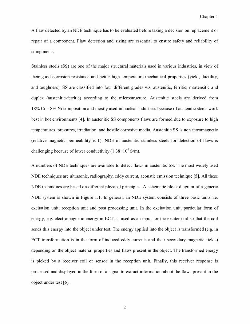
NDE techniques are based on different physical principles. A schematic block diagram of a generic

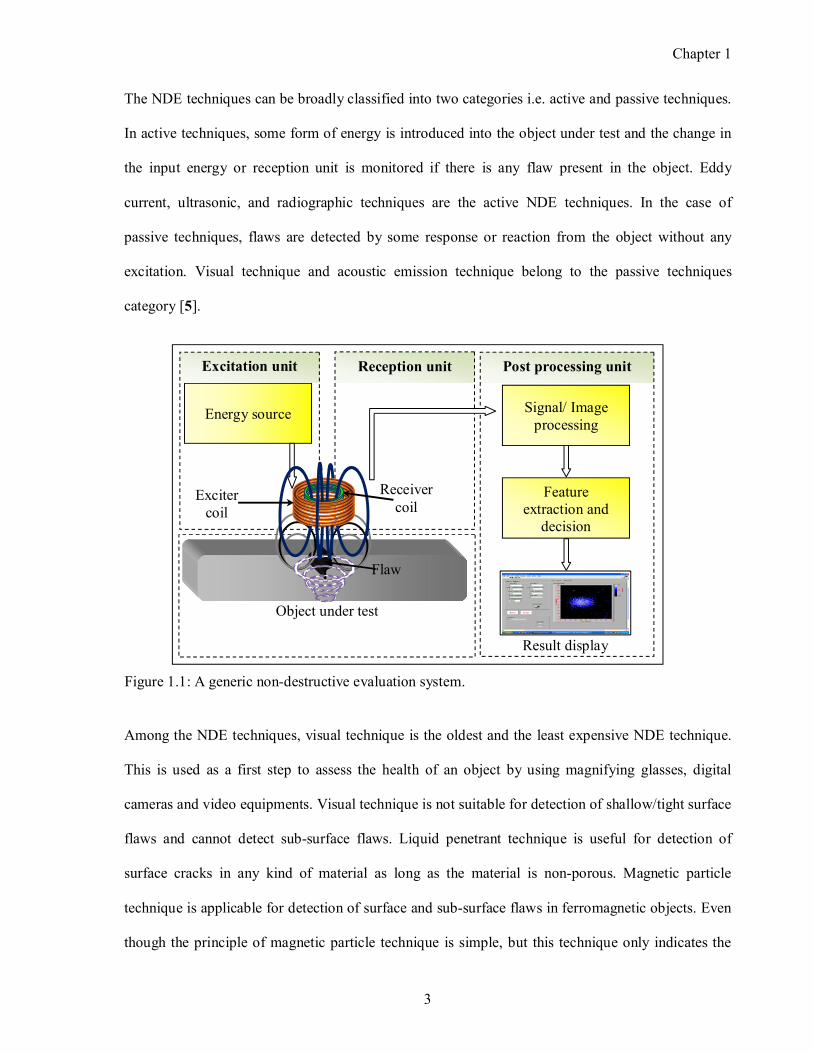
NDE system is shown in Figure 1.1. In general, an NDE system consists of three basic units i.e.

excitation unit, reception unit and post processing unit. In the excitation unit, particular form of

energy, e.g. electromagnetic energy in ECT, is used as an input for the exciter coil so that the coil

sends this energy into the object under test. The energy applied into the object is transformed (e.g. in

ECT transformation is in the form of induced eddy currents and their secondary magnetic fields)

depending on the object material properties and flaws present in the object. The transformed energy

is picked by a receiver coil or sensor in the reception unit. Finally, this receiver response is

processed and displayed in the form of a signal to extract information about the flaws present in the

object under test [6].

Chapter 1

3

The NDE techniques can be broadly classified into two categories i.e. active and passive techniques.

In active techniques, some form of energy is introduced into the object under test and the change in

the input energy or reception unit is monitored if there is any flaw present in the object. Eddy

current, ultrasonic, and radiographic techniques are the active NDE techniques. In the case of

passive techniques, flaws are detected by some response or reaction from the object without any

excitation. Visual technique and acoustic emission technique belong to the passive techniques

category [5].

Among the NDE techniques, visual technique is the oldest and the least expensive NDE technique.

This is used as a first step to assess the health of an object by using magnifying glasses, digital

cameras and video equipments. Visual technique is not suitable for detection of shallow/tight surface

flaws and cannot detect sub­surface flaws. Liquid penetrant technique is useful for detection of

surface cracks in any kind of material as long as the material is non­porous. Magnetic particle

technique is applicable for detection of surface and sub­surface flaws in ferromagnetic objects. Even

though the principle of magnetic particle technique is simple, but this technique only indicates the

Reception unit

Object under test

Post processing unit

Energy source Signal/ Image processing

Feature extraction and

decision

Exciter coil

Receiver coil

Excitation unit

Result display

Flaw

Figure 1.1: A generic non­destructive evaluation system.

Chapter 1

4

presence of a flaw and cannot give any quantitative information. Acoustic emission and infrared

thermography techniques are dynamic techniques and are used for detection of growing cracks, leaks

and hot spots respectively. Radiography technique is widely used for volumetric inspection of

castings, welds, bonded structures, electronic components and composite materials. This technique

requires access from both sides. Compared to other NDE techniques radiography technique is

expensive and proper safety, precautions are required for inspection because of the use of X­rays or

γ­rays. Ultrasonic technique is the most versatile active NDE technique. This technique uses high

frequency (0.5 to 25 MHz) ultrasound energy for dimensional measurements, flaw detection and

microstructure characterisation. This technique requires coupling medium to introduce the sound

energy into the material and cannot be used for laminated or layered structures. Skilled operators are

required to perform ultrasonic inspections. ECT is a widely used electromagnetic NDE (ENDE)

technique for detection and sizing of surface as well as near sub­surface flaws in electrically

conducting materials. In this technique, detection of flaws is confirmed by measuring the changes in

impedance of a coil excited with an alternating current. This is a simple and portable NDE technique

used for inspection of components made of metallic materials.

A single NDE technique cannot detect all types of flaws. Each of the NDE techniques has its own

advantages and limitations as compared to other NDE techniques. For selection of a suitable NDE

technique, the material properties, details of the expected flaws, manufacturing process, environment

surrounding of the components, accessibility, and cost as well as capability of the selected technique

are to be considered.

Among the NDE techniques, ENDE techniques are mostly used for detection of flaws in thin

(thickness ≤ 5.0 mm) electrical conducting materials, such as stainless steel, aluminum, inconel,

brass and copper, etc. [7]. ECT is the extensively used in aerospace, nuclear, petrochemical, and

automobile industries. The main reasons behind the numerous and widespread use of ECT is:

Chapter 1

5

The excellent detection sensitivity for surface as well as near sub­surface flaws (≤ 5.0 mm)

Ease of operation

Versatility

Extremely high testing speeds (up to 10 m/s)

Data storage possibility and

Repeatability.

This technique can detect wall thinning, cracks, pitting, stress corrosion cracking, hydrogen

embrittlement, denting and deposits [8].

1.2 Eddy current testing

Research in eddy currents started with the discovery of electromagnetic induction by Michael

Faraday’s in 1831. Faraday’s stated that the electromagnetic force is generated in a conducting

material if placed in a time varying magnetic field. In 1851 Leon Foucault discovered the

phenomena of eddy currents and showed that eddy currents are generated when a copper disk moves

within an applied magnetic field. The understanding entered into another stage with the discovery of

change in coil properties for different conductivity and permeability metals by David Hughes in

1879. Use of ECT in industries was pioneered by Prof. Friedrich Forster in 1940’s [9].

1.2.1 Principle of eddy current testing

Eddy current technique works on the principle of electromagnetic induction. A schematic of the

working principle of ECT technique is shown in Figure 1.2. When an alternating current (AC) is

applied to a coil (also called probe), primary magnetic field gets generated near the coil following

the Ampere’s law. Due to the primary magnetic field, magnetic flux (��) exists and this is

proportional to the number of turns in the coil (��) and the current �� according to Oersted’s

(i.e. �� ∝ ���� ). When an electrically conducting material, e.g. stainless steel, aluminum, etc. is

Chapter 1

6

placed near the coil, eddy currents are induced in the material according to the Faraday’s law. The

governing differential equation for an eddy current probe excited with alternating current producing

an eddy current density J in a homogeneous isotropic electrically conducting material shown in

Figure 1.2 is derived from the following Maxwell’s curl equations [7]:

∇ × � = − ��

�� (1.1)

∇ × � = − �� (1.2)

where E is the electric field, B is the magnetic field vector, J is the current density and μ is the

magnetic permeability of the material. The governing partial differential equation describing the

ECT technique is given as

∇�� = ����� (1.3)

where ω is the angular excitation frequency and � is the electrical conductivity.

Solving equation 1.3 provides the distribution of the eddy current density (J) in the thickness

direction [10]:

Figure 1.2: Basic principle of the ECT technique.

Test specimen

Induced eddy current

Eddy current probe

Eddy current field

Primary magnetic field

Chapter 1

7

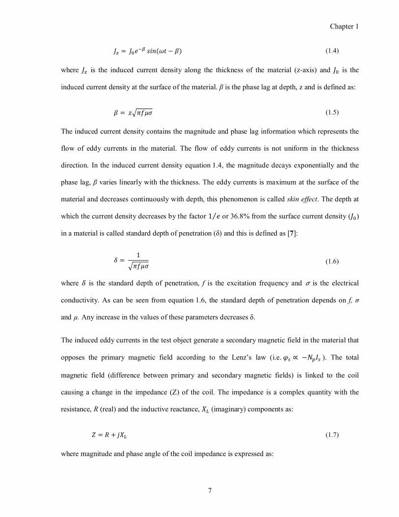
�� = ����� ���(�� − �) (1.4)

where �� is the induced current density along the thickness of the material (z­axis) and �� is the

induced current density at the surface of the material. β is the phase lag at depth, z and is defined as:

� = �� ���� (1.5)

The induced current density contains the magnitude and phase lag information which represents the

flow of eddy currents in the material. The flow of eddy currents is not uniform in the thickness

direction. In the induced current density equation 1.4, the magnitude decays exponentially and the

phase lag, β varies linearly with the thickness. The eddy currents is maximum at the surface of the

material and decreases continuously with depth, this phenomenon is called skin effect. The depth at

which the current density decreases by the factor 1 �⁄ or 36.8% from the surface current density (��)

in a material is called standard depth of penetration (δ) and this is defined as [7]:

� = 1

� ���� (1.6)

where � is the standard depth of penetration, f is the excitation frequency and � is the electrical

conductivity. As can be seen from equation 1.6, the standard depth of penetration depends on f, σ

and µ. Any increase in the values of these parameters decreases δ.

The induced eddy currents in the test object generate a secondary magnetic field in the material that

opposes the primary magnetic field according to the Lenz’s law (i.e. �� ∝ −���� ). The total

magnetic field (difference between primary and secondary magnetic fields) is linked to the coil

causing a change in the impedance (Z) of the coil. The impedance is a complex quantity with the

resistance, R (real) and the inductive reactance, �� (imaginary) components as:

� = � + ��� (1.7)

where magnitude and phase angle of the coil impedance is expressed as:

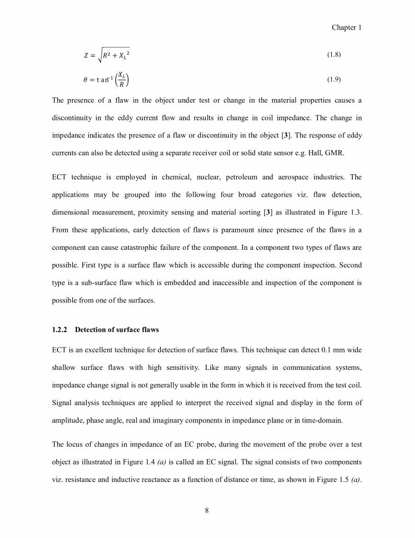
Chapter 1

8

� = ��� + ��� (1.8)

� = tan�� ���

�� (1.9)

The presence of a flaw in the object under test or change in the material properties causes a

discontinuity in the eddy current flow and results in change in coil impedance. The change in

impedance indicates the presence of a flaw or discontinuity in the object [3]. The response of eddy

currents can also be detected using a separate receiver coil or solid state sensor e.g. Hall, GMR.

ECT technique is employed in chemical, nuclear, petroleum and aerospace industries. The

applications may be grouped into the following four broad categories viz. flaw detection,

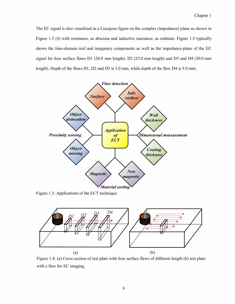
dimensional measurement, proximity sensing and material sorting [3] as illustrated in Figure 1.3.

From these applications, early detection of flaws is paramount since presence of the flaws in a

component can cause catastrophic failure of the component. In a component two types of flaws are

possible. First type is a surface flaw which is accessible during the component inspection. Second

type is a sub­surface flaw which is embedded and inaccessible and inspection of the component is

possible from one of the surfaces.

1.2.2 Detection of surface flaws

ECT is an excellent technique for detection of surface flaws. This technique can detect 0.1 mm wide

shallow surface flaws with high sensitivity. Like many signals in communication systems,

impedance change signal is not generally usable in the form in which it is received from the test coil.

Signal analysis techniques are applied to interpret the received signal and display in the form of

amplitude, phase angle, real and imaginary components in impedance plane or in time­domain.

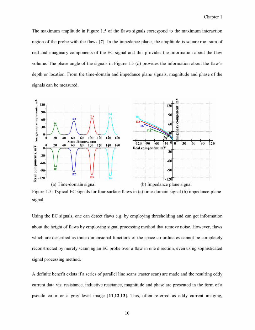
The locus of changes in impedance of an EC probe, during the movement of the probe over a test

object as illustrated in Figure 1.4 (a) is called an EC signal. The signal consists of two components

viz. resistance and inductive reactance as a function of distance or time, as shown in Figure 1.5 (a).

Chapter 1

9

The EC signal is also visualized as a Lissajous figure on the complex (impedance) plane as shown in

Figure 1.5 (b) with resistance, as abscissa and inductive reactance, as ordinate. Figure 1.5 typically

shows the time­domain real and imaginary components as well as the impedance­plane of the EC

signal for four surface flaws D1 (20.0 mm length), D2 (25.0 mm length) and D3 and D4 (30.0 mm

length). Depth of the flaws D1, D2 and D3 is 3.0 mm, while depth of the flaw D4 is 5.0 mm.

(a) (b)

Figure 1.4: (a) Cross section of test plate with four surface flaws of different length (b) test plate

with a flaw for EC imaging.

D1 D2 D3 D4

Figure 1.3: Applications of the ECT technique.

Flaw detection

Material sorting

Dimensional measurement Proximity sensing

Wall thickness

Coating thickness

Surface

Non magnetic

Magnetic

Object dislocation

Object missing

Application of

ECT

Sub-surface

Chapter 1

10

The maximum amplitude in Figure 1.5 of the flaws signals correspond to the maximum interaction

region of the probe with the flaws [7]. In the impedance plane, the amplitude is square root sum of

real and imaginary components of the EC signal and this provides the information about the flaw

volume. The phase angle of the signals in Figure 1.5 (b) provides the information about the flaw’s

depth or location. From the time­domain and impedance plane signals, magnitude and phase of the

signals can be measured.

Using the EC signals, one can detect flaws e.g. by employing thresholding and can get information

about the height of flaws by employing signal processing method that remove noise. However, flaws

which are described as three­dimensional functions of the space co­ordinates cannot be completely

reconstructed by merely scanning an EC probe over a flaw in one direction, even using sophisticated

signal processing method.

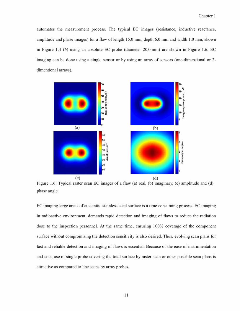
A definite benefit exists if a series of parallel line scans (raster scan) are made and the resulting eddy

current data viz. resistance, inductive reactance, magnitude and phase are presented in the form of a

pseudo color or a gray level image [11,12,13]. This, often referred as eddy current imaging,

(a) Time­domain signal (b) Impedance plane signal

Figure 1.5: Typical EC signals for four surface flaws in (a) time­domain signal (b) impedance­plane

signal.

Chapter 1

11

automates the measurement process. The typical EC images (resistance, inductive reactance,

amplitude and phase images) for a flaw of length 15.0 mm, depth 6.0 mm and width 1.0 mm, shown

in Figure 1.4 (b) using an absolute EC probe (diameter 20.0 mm) are shown in Figure 1.6. EC

imaging can be done using a single sensor or by using an array of sensors (one­dimensional or 2­

dimentional arrays).

EC imaging large areas of austenitic stainless steel surface is a time consuming process. EC imaging

in radioactive environment, demands rapid detection and imaging of flaws to reduce the radiation

dose to the inspection personnel. At the same time, ensuring 100% coverage of the component

surface without compromising the detection sensitivity is also desired. Thus, evolving scan plans for

fast and reliable detection and imaging of flaws is essential. Because of the ease of instrumentation

and cost, use of single probe covering the total surface by raster scan or other possible scan plans is

attractive as compared to line scans by array probes.

(a) (b)

(d) (c) Figure 1.6: Typical raster scan EC images of a flaw (a) real, (b) imaginary, (c) amplitude and (d)

phase angle.

Chapter 1

12

1.2.3 Detection of sub-surface flaws

The ECT technique is in general, confined to detection of sub­surface flaws within a depth of

5.0 mm in austenitic stainless steels. Components such as storage tanks, dissolver vessels etc. are

made with thick stainless steel plates in the range of 8.0 mm to 12.0 mm. This type of components is

used in petrochemical industries and nuclear reprocessing plants for storage and transportation of

different chemicals. In nuclear reprocessing plants, storage tanks are used to store the radioactive

liquid waste in nitric acid medium arising from the reprocessing operations. These tanks are made of

AISI type 304L austenitic stainless steel. This steel undergoes several types of corrosion namely

end­grain attack, uniform corrosion, tunnelling corrosion, transpassive dissolution [14,15]. Periodic

non­destructive inspection of these components for detection of corrosion is required to ensure the

structural integrity and to continue to use. Due to the radiation environment, inspection of the tanks

from inner surface is not possible and detection of inside (deep sub­surface) flaws and corrosion

damage from the outer surface is challenging for the ECT technique.

1.3 Considarations for detection of sub-surface flaws

There are some factors which influence the capability of ECT technique for detection of sub­surface

flaws. Penetration of eddy currents into the material upto the flaw location is essential, since the

change in impedance occurs only when eddy currents are disturbed by the flaw. As the standard

depth of penetration is limited by the material properties and excitation frequency, this behavior

cannot be changed fundamentally. But by the optimization of ECT probes and testing parameters,

enhanced penetration can be achieved and this penetration is called the effective depth of

penetration, (�� ). This is the depth at which eddy current density decreases to 1 ��⁄ or 4.9% of the

surface current density. Beyond this depth change in coil impedance is negligible [16,17]. The

effective depth of penetration is also the depth upto which eddy current signals are received with

sufficient signal to noise ratio (SNR) [18] which depends on the test material, instrument, probe,

Chapter 1

13

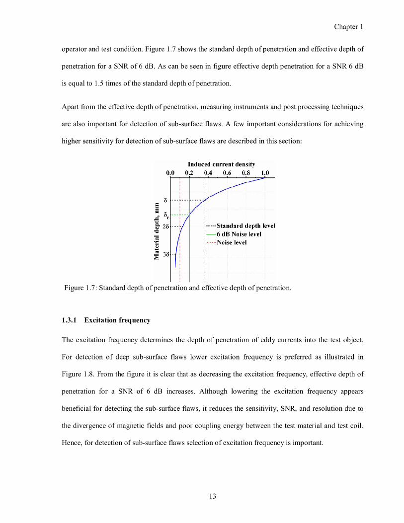
operator and test condition. Figure 1.7 shows the standard depth of penetration and effective depth of

penetration for a SNR of 6 dB. As can be seen in figure effective depth penetration for a SNR 6 dB

is equal to 1.5 times of the standard depth of penetration.

Apart from the effective depth of penetration, measuring instruments and post processing techniques

are also important for detection of sub­surface flaws. A few important considerations for achieving

higher sensitivity for detection of sub­surface flaws are described in this section:

1.3.1 Excitation frequency

The excitation frequency determines the depth of penetration of eddy currents into the test object.

For detection of deep sub­surface flaws lower excitation frequency is preferred as illustrated in

Figure 1.8. From the figure it is clear that as decreasing the excitation frequency, effective depth of

penetration for a SNR of 6 dB increases. Although lowering the excitation frequency appears

beneficial for detecting the sub­surface flaws, it reduces the sensitivity, SNR, and resolution due to

the divergence of magnetic fields and poor coupling energy between the test material and test coil.

Hence, for detection of sub­surface flaws selection of excitation frequency is important.

Figure 1.7: Standard depth of penetration and effective depth of penetration.

Chapter 1

14

1.3.2 Electromagnetic coupling

Electromagnetic coupling between the test coil and the object under test is very important during

inspection, because it decides the interaction between the test coil and the object. Lift­off, fill­factor,

edge­effect and end­effect describe the electromagnetic coupling. The coupling between the test coil

and object under test varies with the spacing between the test coil and the test object and this spacing

is called ‘lift­off’ for inspections using the pancake probes and called ‘fill­factor’ for inspections

using the bobbin probes [3]. Variation in coupling due to change in lift­off results in noisy signal,

generally termed as lift­off signal or wobble signal that disturbs the inspection. During ECT, zero

lift­off or uniform lift­off is preferred and usually, the lift­off signal is made parallel to the X­axis on

the impedance plane display for reference as well as for phase discrimination purpose. The use of

spring loaded surface probes ensure good electromagnetic coupling and this reduces disturbing

signals from variations in lift­off.

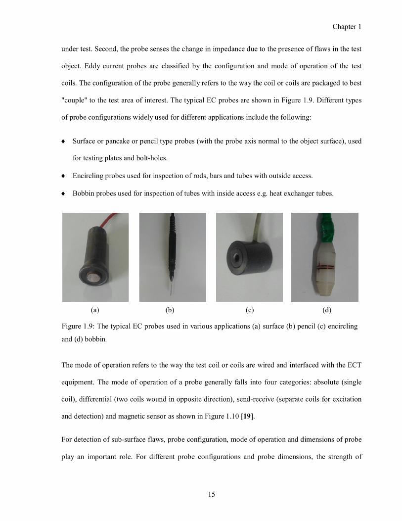
1.3.3 Eddy current probe

Probe is the main link between the EC instrument and the test object and it has two main functions.

First, the EC probe establishes varying electromagnetic fields that induce eddy currents in the object

Figure 1.8: Standard and effective depth of penetration with varying frequency.

Chapter 1

15

under test. Second, the probe senses the change in impedance due to the presence of flaws in the test

object. Eddy current probes are classified by the configuration and mode of operation of the test

coils. The configuration of the probe generally refers to the way the coil or coils are packaged to best

"couple" to the test area of interest. The typical EC probes are shown in Figure 1.9. Different types

of probe configurations widely used for different applications include the following:

Surface or pancake or pencil type probes (with the probe axis normal to the object surface), used

for testing plates and bolt­holes.

Encircling probes used for inspection of rods, bars and tubes with outside access.

Bobbin probes used for inspection of tubes with inside access e.g. heat exchanger tubes.

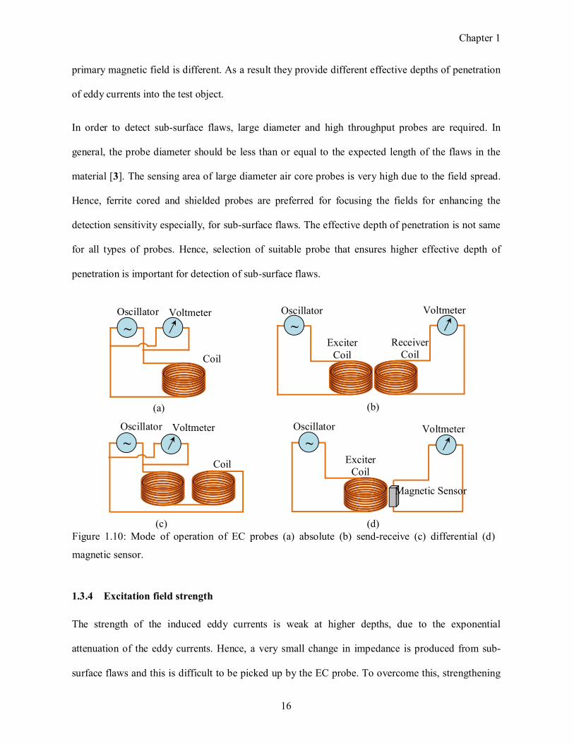
The mode of operation refers to the way the test coil or coils are wired and interfaced with the ECT

equipment. The mode of operation of a probe generally falls into four categories: absolute (single

coil), differential (two coils wound in opposite direction), send­receive (separate coils for excitation

and detection) and magnetic sensor as shown in Figure 1.10 [19].

For detection of sub­surface flaws, probe configuration, mode of operation and dimensions of probe

play an important role. For different probe configurations and probe dimensions, the strength of

(a) (b) (c)

Figure 1.9: The typical EC probes used in various applications (a) surface (b) pencil (c) encircling

and (d) bobbin.

(d)

Chapter 1

16

primary magnetic field is different. As a result they provide different effective depths of penetration

of eddy currents into the test object.

In order to detect sub­surface flaws, large diameter and high throughput probes are required. In

general, the probe diameter should be less than or equal to the expected length of the flaws in the

material [3]. The sensing area of large diameter air core probes is very high due to the field spread.

Hence, ferrite cored and shielded probes are preferred for focusing the fields for enhancing the

detection sensitivity especially, for sub­surface flaws. The effective depth of penetration is not same

for all types of probes. Hence, selection of suitable probe that ensures higher effective depth of

penetration is important for detection of sub­surface flaws.

1.3.4 Excitation field strength

The strength of the induced eddy currents is weak at higher depths, due to the exponential

attenuation of the eddy currents. Hence, a very small change in impedance is produced from sub­

surface flaws and this is difficult to be picked up by the EC probe. To overcome this, strengthening

Figure 1.10: Mode of operation of EC probes (a) absolute (b) send­receive (c) differential (d)

magnetic sensor.

(a) (b)

(c) (d)

~

Oscillator Voltmeter

Coil

~

Oscillator Voltmeter

Exciter Coil

Receiver Coil

~

Oscillator Voltmeter

Coil

~

Oscillator Voltmeter

Exciter Coil

Magnetic Sensor

Chapter 1

17

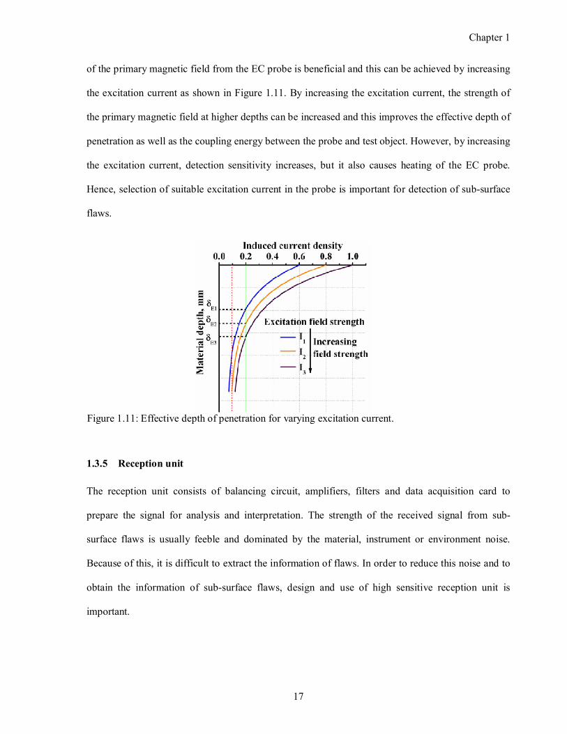
of the primary magnetic field from the EC probe is beneficial and this can be achieved by increasing

the excitation current as shown in Figure 1.11. By increasing the excitation current, the strength of

the primary magnetic field at higher depths can be increased and this improves the effective depth of

penetration as well as the coupling energy between the probe and test object. However, by increasing

the excitation current, detection sensitivity increases, but it also causes heating of the EC probe.

Hence, selection of suitable excitation current in the probe is important for detection of sub­surface

flaws.

1.3.5 Reception unit

The reception unit consists of balancing circuit, amplifiers, filters and data acquisition card to

prepare the signal for analysis and interpretation. The strength of the received signal from sub­

surface flaws is usually feeble and dominated by the material, instrument or environment noise.

Because of this, it is difficult to extract the information of flaws. In order to reduce this noise and to

obtain the information of sub­surface flaws, design and use of high sensitive reception unit is

important.

Figure 1.11: Effective depth of penetration for varying excitation current.

Chapter 1

18

1.3.6 Processing of Signals and images

In order to minimise noise introduced in the EC signals due to surface roughness, probe tilt,

variation in lift­off and instrumentation noise and also to extract useful information of flaws, various

signal processing technique are employed. These include use of filters, artificial neural networks,

Fourier analysis, wavelet analysis, principal component analysis (PCA), multi­frequency analysis

etc. [20,21,22,23].

The information obtained from a single line­scan of an EC probe is limited. In order to extract

quantitative information of flaws imaging is essential and processing of eddy current images is

important for removing noise, identification of regions of flaws and characterization of flaws. Use of

several image processing methods time­based, frequency­based, wavelet based is common in ECT.

For detection of sub­surface flaws, use of larger diameter probe excited with lower frequency is

required. EC images of large diameter probes at lower frequency suffer from blurring or over sizing

due to the large foot print or point spread function (psf) of the EC probe which decreases the

resolution and SNR [3].

1.3.7 Fusion of images

NDE is an application field that lends itself naturally to data fusion largely because it involves the

use of multiple sensors by different NDE techniques. NDE data fusion methods utilize the

redundancy and complementary information from different sensors, frequency and techniques to

enhance the resulting image. Image fusion is a process of combining relevant information from two

or more images into a single image and the fused image is expected to be more informative than any

of the input images. The reliability of ECT technique can be improved through the combination of

redundant information, as well as through the fusion of complementary information. The redundant

information is used to improve the SNR of the images and the complementary information is used to

augment the overall information content, which in turn, increases the accuracy of sizing. NDE fusion

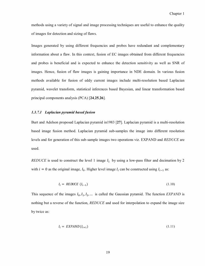
Chapter 1

19

methods using a variety of signal and image processing techniques are useful to enhance the quality

of images for detection and sizing of flaws.

Images generated by using different frequencies and probes have redundant and complementary

information about a flaw. In this context, fusion of EC images obtained from different frequencies

and probes is beneficial and is expected to enhance the detection sensitivity as well as SNR of

images. Hence, fusion of flaw images is gaining importance in NDE domain. In various fusion

methods available for fusion of eddy current images include multi­resolution based Laplacian

pyramid, wavelet transform, statistical inferences based Bayesian, and linear transformation based

principal components analysis (PCA) [24,25,26].

1.3.7.1 Laplacian pyramid based fusion

Burt and Adelson proposed Laplacian pyramid in1983 [27]. Laplacian pyramid is a multi­resolution

based image fusion method. Laplacian pyramid sub­samples the image into different resolution

levels and for generation of this sub­sample images two operations viz. EXPAND and REDUCE are

used.

REDUCE is used to construct the level 1 image �� by using a low­pass filter and decimation by 2

with � = 0 as the original image, ��. Higher level image �� can be constructed using ���� as:

�� = ������ (����) (1.10)

This sequence of the images ��,��,��,… is called the Gaussian pyramid. The function EXPAND is

nothing but a reverse of the function, REDUCE and used for interpolation to expand the image size

by twice as:

�� = ������ (��� �) (1.11)

Chapter 1

20

Laplacian pyramid is a sequence of the residual images which is a difference of the expanded ��� �

image and image �� as define by:

����������� = ���� – ������ (�� ) (1.12)

The Laplacian pyramid images contain the information regarding the edges of the images and in case

of ECT, the knowledge about the total area of flaws is important for flaw sizing [28]. Hence,

Laplacian pyramid based image fusion is attractive for detection of sub­surface flaws. For fusion of

images, Laplacian pyramid of two images can be fused by the pixel­based method and typical

schematic diagram is shown in Figure 1.12. Reconstruction of the fused Laplacian pyramid images

can be obtained by the combination of the expanded images and residual images as:

�� = ������ (��� �) + ��������� (1.13)

1.3.7.2 Wavelet transform based fusion

Wavelet transform decomposes an image into four coefficients namely, low­low (LL), low­high

(LH), high­low (HL) and high­high (HH) by separately filtering and down sampling using the low

Figure 1.12: Schematic diagram of Laplacian transform based image fusion.

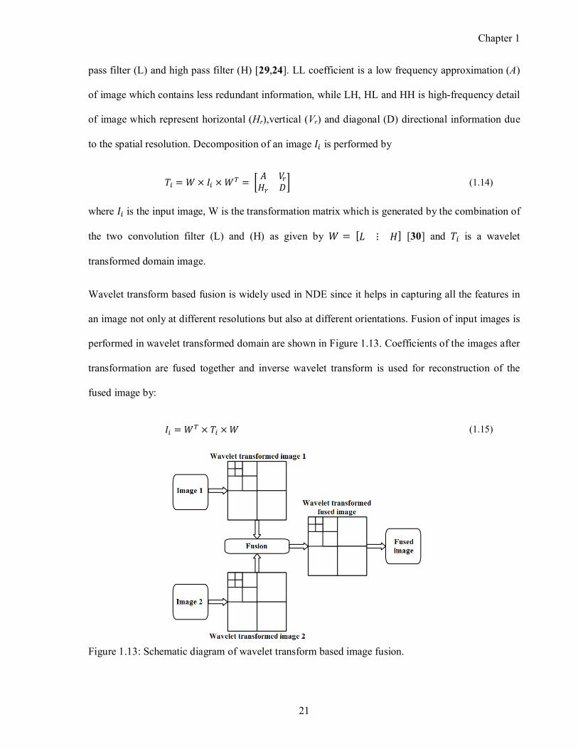
Chapter 1

21

pass filter (L) and high pass filter (H) [29,24]. LL coefficient is a low frequency approximation (A)

of image which contains less redundant information, while LH, HL and HH is high­frequency detail

of image which represent horizontal (Hr),vertical (Vr) and diagonal (D) directional information due

to the spatial resolution. Decomposition of an image �� is performed by

�� = � × �� × �� = �� ��

�� �� (1.14)

where �� is the input image, W is the transformation matrix which is generated by the combination of

the two convolution filter (L) and (H) as given by � = [� ⋮ �] [30] and �� is a wavelet

transformed domain image.

Wavelet transform based fusion is widely used in NDE since it helps in capturing all the features in

an image not only at different resolutions but also at different orientations. Fusion of input images is

performed in wavelet transformed domain are shown in Figure 1.13. Coefficients of the images after

transformation are fused together and inverse wavelet transform is used for reconstruction of the

fused image by:

�� = �� × �� × � (1.15)

Figure 1.13: Schematic diagram of wavelet transform based image fusion.

Chapter 1

22

1.3.7.3 Bayesian based fusion

Bayesian fusion works on the principle Bayes rule which is based on the statistical inferences and

probability theory. Bayes rule divides the statisticians over the idea of how best to estimate an

unknown parameter from a set of data [31]. For example, if it is desired to identify a flaw based on a

set of measurements of useful parameters, from this data set one must extract the best value of some

quantity. In order to achieve the best value, fusion method involves formulating the fusion problem

in probabilities [32] and for this, the input images are assumed to be independent events with the

likelihood of images I1… IN is given by

�(��,… ,��|�) = � �(��|�)

�

���

(1.16)

where p(θ) is the prior and known knowledge about occurrence of flaw. The posterior distribution

according to the Bayes principle, is given by

�(��|��,… ,��) ∝ �(�)� �(��|�)

�

���

(1.17)

It is well know that in ECT, the image of flaw appears in the form of Gaussian function, as eddy

current probe and point spread function are circular. Hence, formulation of the prior probability for

Bayesian fusion normal Gaussian distribution with zero mean and unit standard deviation is moved

over the input images to find the best fit Gaussian distribution matrix. The individual pixel values of

the input images are taken as the likelihood and the posterior distribution gives the information about

the features in the fused images.

1.3.7.4 Principal components analysis based fusion

Principal component analysis (PCA) is a linear transformation method which involves a

mathematical procedure that transforms a number of correlated variables into a number of

uncorrelated variables called principal components [29]. In general, the first principal component

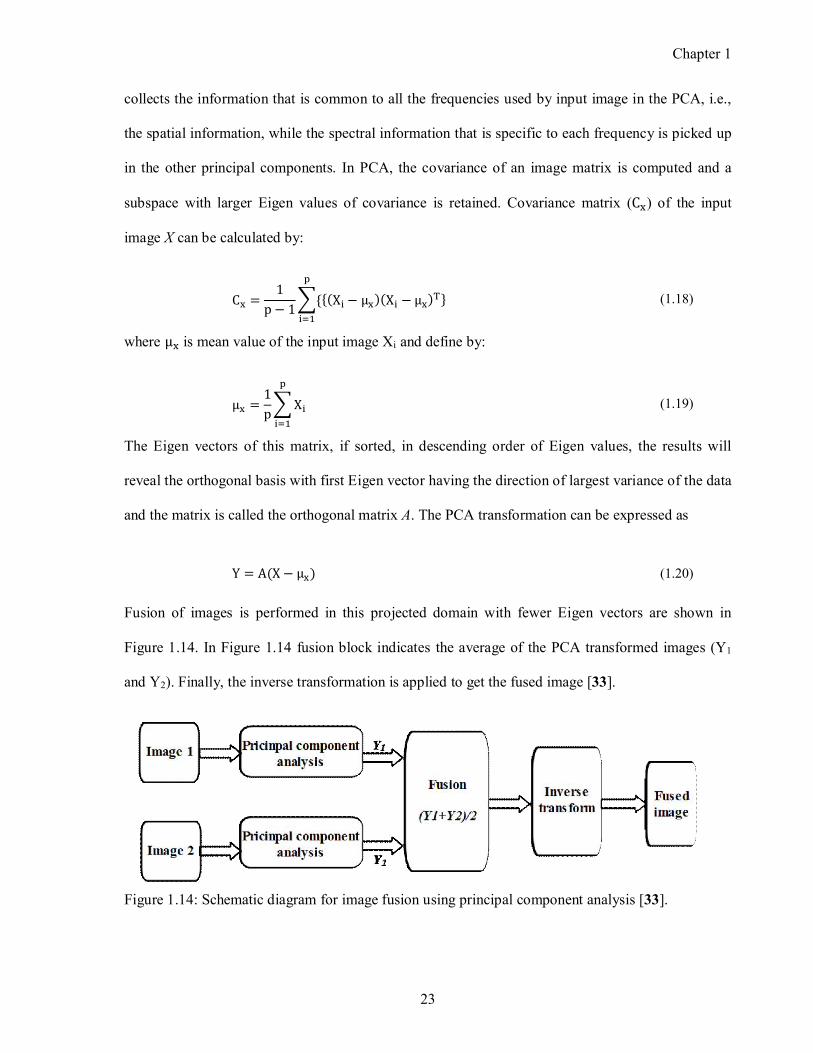
Chapter 1

23

collects the information that is common to all the frequencies used by input image in the PCA, i.e.,

the spatial information, while the spectral information that is specific to each frequency is picked up

in the other principal components. In PCA, the covariance of an image matrix is computed and a

subspace with larger Eigen values of covariance is retained. Covariance matrix (C�) of the input

image X can be calculated by:

C� =1

p − 1�{{(X� − μ�)(X� − μ�)�}

�

���

(1.18)

where μ� is mean value of the input image Xi and define by:

μ� =1

p� X�

�

���

(1.19)

The Eigen vectors of this matrix, if sorted, in descending order of Eigen values, the results will

reveal the orthogonal basis with first Eigen vector having the direction of largest variance of the data

and the matrix is called the orthogonal matrix A. The PCA transformation can be expressed as

Y = A(X − μ�) (1.20)

Fusion of images is performed in this projected domain with fewer Eigen vectors are shown in

Figure 1.14. In Figure 1.14 fusion block indicates the average of the PCA transformed images (Y1

and Y2). Finally, the inverse transformation is applied to get the fused image [33].

Figure 1.14: Schematic diagram for image fusion using principal component analysis [33].

Chapter 1

24

X = A�Y + μ� (1.21)

1.4 Litera ture review

As discussed in Section 1.3, enhancement in detection of sub­surface flaws is possible by selection

of suitable EC probes and optimization of test parameters. Several approaches including

development of high throughput probes, better instruments and processing of eddy current signals

and images have been attempted by many researchers earlier for enhanced detection of sub­surface

flaws.

1.4.1 Eddy current probe

For detection of sub­surface flaws using ECT, it is important to design an optimum probe

configuration. In this context, there is a strong need to study the different probe configurations to

design a suitable probe for detection of sub­surface flaws. This could be accomplished either by

experimentation or by numerical modelling. Various researchers studied different probe

configurations and mode of operation for detection of flaws, flaw orientation, wall thickness etc

[34,35,36,37,38,39]. ECT is used extensively for inspection of steam generator tubes in nuclear

power plants. For inspection of steam generator tubes, different types of probes were used [40,41].

In the literature, use of air core, ferrite core, inductive, E­core, Double­D, cup­core type probe

configurations was represented.

Palanisamy et al (1983) studied the influence of absolute EC coil with and without ferrite core (i.e.

cup­core and air core) using finite element (FE) model for detection and characterisation of flaws in

a disk bolt holes under a 1.27 mm SS sleeve. In this study, change in impedance of probe coil and

distribution of eddy currents around a flaw in the second layer (1.27 mm below) of aluminium lap

joint were predicted. They noted that the detection sensitivity of air core coil is higher for smaller

coils (i.e. mean radius, �� < 1.0 ��) and for larger mean radius (�� > 1.0 ��), cup­core coil is

Chapter 1

25

more sensitive than air core coil. They also reported that cup­core coil provides better signal

resolution than air core coil due to the focused flux interaction [42].

Hoshikawa et al (1984) compared the performance of absolute and send­receive mode probes using

FE model. For these studies 4.0, 10.0 and 30.0 mm diameter absolute single coil probe and send­

receive mode double coil probe with 30.0 mm excitation coil and 4.0 mm pick­up coil were used.

Cross section of these coils is shown in Figure 1.15. The change of impedance and induced voltage

response of the probes were calculated as a function of lift­off variation and flat bottom hole depth

as shown in Figure 1.16. It was found that for double coil probe the change of impedance and

induced voltage due to lift­off and flat bottom hole depth was far larger than that of the absolute coil

probe and send­receive mode double coil probe [43].

(a) (b) Figure 1.16: Predicted change rates of impedance and induced voltage due to (a) lift off change

(b) flat bottom hole depth change [43].

Figure 1.15: Cross section of surface probe over a conducting surface (a) small diameter single

coil (b) large diameter single coil and (c) double coil probe [43].

(a) (b) (c)

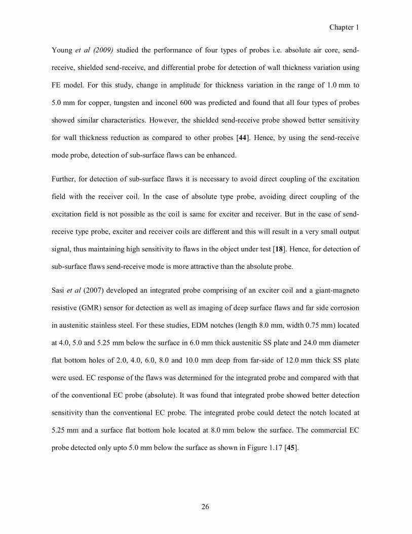
Chapter 1

26

Young et al (2009) studied the performance of four types of probes i.e. absolute air core, send­

receive, shielded send­receive, and differential probe for detection of wall thickness variation using

FE model. For this study, change in amplitude for thickness variation in the range of 1.0 mm to

5.0 mm for copper, tungsten and inconel 600 was predicted and found that all four types of probes

showed similar characteristics. However, the shielded send­receive probe showed better sensitivity

for wall thickness reduction as compared to other probes [44]. Hence, by using the send­receive

mode probe, detection of sub­surface flaws can be enhanced.

Further, for detection of sub­surface flaws it is necessary to avoid direct coupling of the excitation

field with the receiver coil. In the case of absolute type probe, avoiding direct coupling of the

excitation field is not possible as the coil is same for exciter and receiver. But in the case of send­

receive type probe, exciter and receiver coils are different and this will result in a very small output

signal, thus maintaining high sensitivity to flaws in the object under test [18]. Hence, for detection of

sub­surface flaws send­receive mode is more attractive than the absolute probe.

Sasi et al (2007) developed an integrated probe comprising of an exciter coil and a giant­magneto

resistive (GMR) sensor for detection as well as imaging of deep surface flaws and far side corrosion

in austenitic stainless steel. For these studies, EDM notches (length 8.0 mm, width 0.75 mm) located

at 4.0, 5.0 and 5.25 mm below the surface in 6.0 mm thick austenitic SS plate and 24.0 mm diameter

flat bottom holes of 2.0, 4.0, 6.0, 8.0 and 10.0 mm deep from far­side of 12.0 mm thick SS plate

were used. EC response of the flaws was determined for the integrated probe and compared with that

of the conventional EC probe (absolute). It was found that integrated probe showed better detection

sensitivity than the conventional EC probe. The integrated probe could detect the notch located at

5.25 mm and a surface flat bottom hole located at 8.0 mm below the surface. The commercial EC

probe detected only upto 5.0 mm below the surface as shown in Figure 1.17 [45].

Chapter 1

27

Angani et al (2011) developed a differential Hall sensor based ferrite core probe for detection of

sub­surface flaws in insulated thick SS pipes. In the differential probe, two Hall sensors were placed

at top and bottom axial center of the excitation coil. For this study, SS plate of thickness 8.0 mm

with artificial notches located at 1.0 mm to 5.0 mm below the surface was used. A plastic sheet with

thickness of 4.0 mm was placed over the surface of the plate to simulate the thermal insulation of the

pipeline [46]. A real time LabVIEW based scanning was used at 500 mA excitation current and

response of the probe was acquired as shown in Figure 1.18. They reported that the differential

probe had the potential to detect sub­surface flaws in insulated pipelines.

Figure 1.18: Differential Hall sensor probe response for sample having EDM notches at different

depths [46].

(a) (b) Figure 1.17: Response of integrated EC GMR sensor and pancake type absolute EC sensor signal

from (a) EDM notches (b) the sensor output for flat bottom hole located at different depths [45].

Chapter 1

28

It is noticed that solid state sensors are useful to improve the detection sensitivity. However, for use

in radioactive conditions, solid state sensors such as Hall and GMR are not suitable, as they undergo

radiation damage [47]. On the other hand, the traditional coil based eddy current probes are well

suited, in view of their large dynamic range, good radiation resistance, slow degradation, better

stability, and low­cost, despite their lower sensitivity as compared to the solid state sensors.

Attempts have been made earlier by many researchers towards improving the sensitivity of the coil

based probes by employing magnetic shielding and circuits. For analysis of ferrite core probes, FE

model was used and induced current density and probe impedance were evaluated for performance

assessment [48,49,50].

Vernon et al (1987) studied the influence of shielding on detection sensitivity by using self­shielding

(by coil shielding) and imposed shielding (by ferrite core) configurations in absolute mode.

Sensitivity of the probe was predicted in term of coupling coefficient between the probe and the

material (aluminium and carbon/carbon). The coupling coefficient was calculated for lift­off

variation and by changing the coil winding. It was found that the imposed shielding increases the

sensitivity of the probe [51].

Joubert et al (2010) developed a cup­core probe with four flat pick­up array coils for detection of

sub­surface flaws in rivets located 4.0 mm below the surface in a 10.0 mm thick aluminium plate

[52]. The pick­up coils comprise of 32 turns distributed in 8 layers of printed circuit board (PCB)

and cover an angular sector of 90 degrees. Differential trans­impedance of the probe due to sub­

surface flaws was measured and it was noted that the cup­core array probe showed good sensitivity

for flaws oriented at different angles.

From the literature, it is learnt that the send­receive mode probe coil appears good for detection of

sub­surface flaws in austenitic SS. Shielding of the probe is expected to provide better coupling

between the probe and test object.

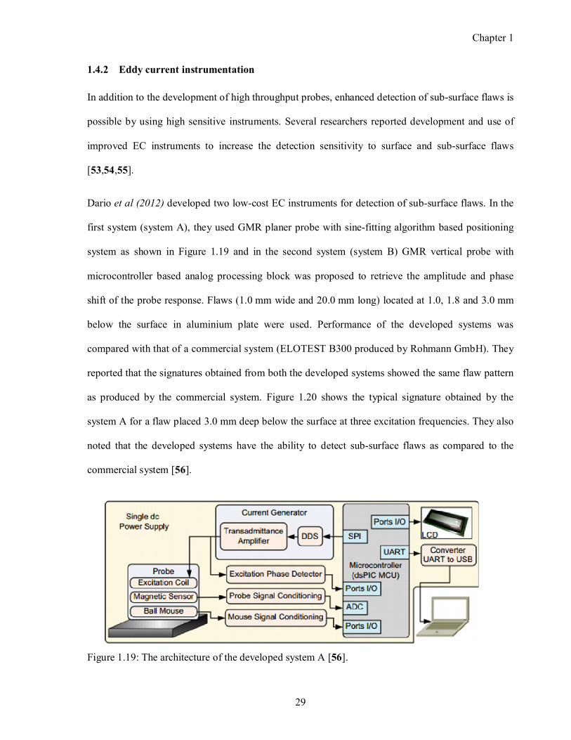
Chapter 1

29

1.4.2 Eddy current instrumentation

In addition to the development of high throughput probes, enhanced detection of sub­surface flaws is

possible by using high sensitive instruments. Several researchers reported development and use of

improved EC instruments to increase the detection sensitivity to surface and sub­surface flaws

[53,54,55].

Dario et al (2012) developed two low­cost EC instruments for detection of sub­surface flaws. In the

first system (system A), they used GMR planer probe with sine­fitting algorithm based positioning

system as shown in Figure 1.19 and in the second system (system B) GMR vertical probe with

microcontroller based analog processing block was proposed to retrieve the amplitude and phase

shift of the probe response. Flaws (1.0 mm wide and 20.0 mm long) located at 1.0, 1.8 and 3.0 mm

below the surface in aluminium plate were used. Performance of the developed systems was

compared with that of a commercial system (ELOTEST B300 produced by Rohmann GmbH). They

reported that the signatures obtained from both the developed systems showed the same flaw pattern

as produced by the commercial system. Figure 1.20 shows the typical signature obtained by the

system A for a flaw placed 3.0 mm deep below the surface at three excitation frequencies. They also

noted that the developed systems have the ability to detect sub­surface flaws as compared to the

commercial system [56].

Figure 1.19: The architecture of the developed system A [56].

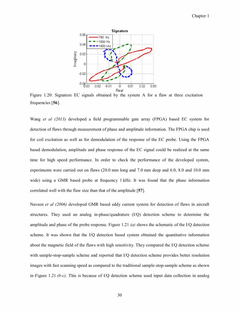
Chapter 1

30

Wang et al (2013) developed a field programmable gate array (FPGA) based EC system for

detection of flaws through measurement of phase and amplitude information. The FPGA chip is used

for coil excitation as well as for demodulation of the response of the EC probe. Using the FPGA

based demodulation, amplitude and phase response of the EC signal could be realized at the same

time for high speed performance. In order to check the performance of the developed system,

experiments were carried out on flaws (20.0 mm long and 7.0 mm deep and 6.0, 8.0 and 10.0 mm

wide) using a GMR based probe at frequency 1 kHz. It was found that the phase information

correlated well with the flaw size than that of the amplitude [57].

Naveen et al (2006) developed GMR based eddy current system for detection of flaws in aircraft

structures. They used an analog in­phase/quadrature (I/Q) detection scheme to determine the

amplitude and phase of the probe response. Figure 1.21 (a) shows the schematic of the I/Q detection

scheme. It was shown that the I/Q detection based system obtained the quantitative information

about the magnetic field of the flaws with high sensitivity. They compared the I/Q detection scheme

with sample­stop­sample scheme and reported that I/Q detection scheme provides better resolution

images with fast scanning speed as compared to the traditional sample­stop­sample scheme as shown

in Figure 1.21 (b-c). This is because of I/Q detection scheme used input data collection in analog

Figure 1.20: Signature EC signals obtained by the system A for a flaw at three excitation

frequencies [56].

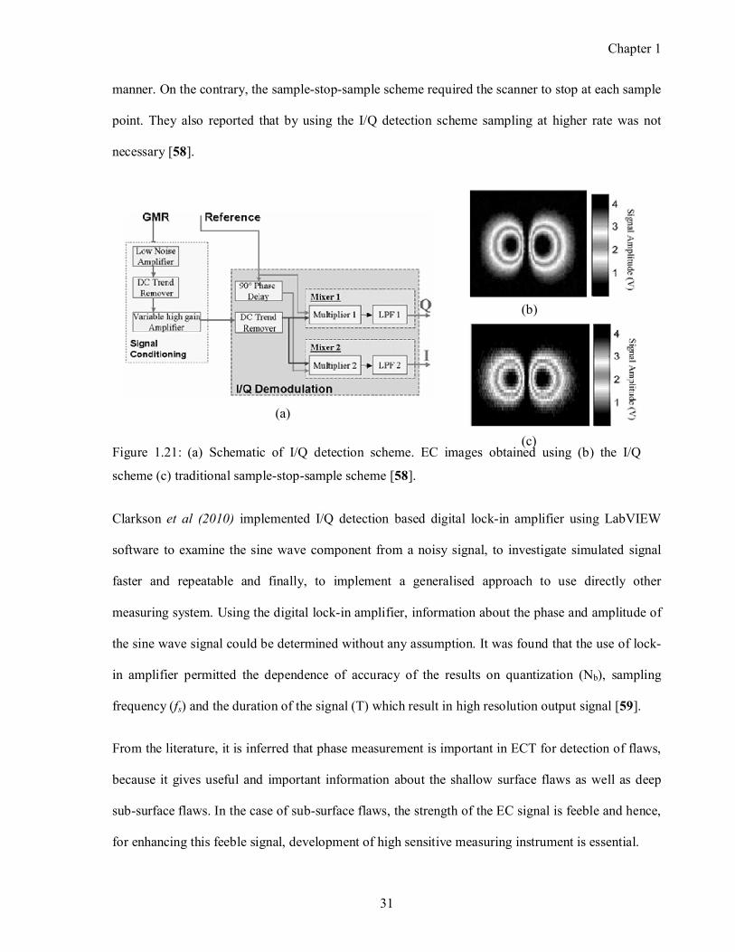
Chapter 1

31

manner. On the contrary, the sample­stop­sample scheme required the scanner to stop at each sample

point. They also reported that by using the I/Q detection scheme sampling at higher rate was not

necessary [58].

Clarkson et al (2010) implemented I/Q detection based digital lock­in amplifier using LabVIEW

software to examine the sine wave component from a noisy signal, to investigate simulated signal

faster and repeatable and finally, to implement a generalised approach to use directly other

measuring system. Using the digital lock­in amplifier, information about the phase and amplitude of

the sine wave signal could be determined without any assumption. It was found that the use of lock­

in amplifier permitted the dependence of accuracy of the results on quantization (Nb), sampling

frequency (fs) and the duration of the signal (T) which result in high resolution output signal [59].

From the literature, it is inferred that phase measurement is important in ECT for detection of flaws,

because it gives useful and important information about the shallow surface flaws as well as deep

sub­surface flaws. In the case of sub­surface flaws, the strength of the EC signal is feeble and hence,

for enhancing this feeble signal, development of high sensitive measuring instrument is essential.

(a)

Figure 1.21: (a) Schematic of I/Q detection scheme. EC images obtained using (b) the I/Q

scheme (c) traditional sample­stop­sample scheme [58].

(b)

(c)

Chapter 1

32

1.4.3 Signal and image processing

1.4.3.1 Signal processing

Doctor et al. proposed non­parametric classification methods based on feature­extraction techniques,

which first create a feature vector containing elements drawn from time, frequency and spatial

domain and then apply pattern recognition methods for classification of flaws [60]. Udpa et al. used

a few invariant Fourier descriptors to estimate depth of flaws in heat exchanger tubes and under

support plates with reasonable success [61]. Shyamsunder et al. used the time­domain and the

frequency­domain parameter of signals from line scans in different orientations for classification of

surface flaws. The best parameters were chosen by using a Fischer statistical ranking and

classification was carried out using an artificial neural network [62]. Joubert et al proposed principal

component analysis and independent component analysis based signal processing approaches for

improvement in detection of sub­surface flaws [52]. Thirunavukkarasu et al. used Fourier filtering,

cross­correlation, and continuous wavelet transform based techniques for detection of flaws in

expansion bend regions of modified 9Cr–1Mo steam generator tubes of sodium cooled fast breeder

reactor. They found that Fourier filtering, cross­correlation techniques can reduce the noise and

detect 20% wall thickness grooves in tube. They reported that continuous wavelet transform based

technique unambiguously detected 10% WT deep grooves present anywhere in the bend regions

with a SNR better than 7 dB [20].

1.4.3.2 Image processing

Xiang et al. implemented an automated signal analysis algorithm for eddy current data from steam

generator tubes. The algorithm converts the data into a visually appealing format and analyses it to

determine the presence or absence of flaws. They also proposed a blind deconvolution algorithm to

detect and accurately size flaws [21]. Kalyansundaram et al. proposed an Eigen value based

approach for enhancement of eddy current images. In this approach, Eigen pairs having maximum

Chapter 1

33

information of the impedance change due to the flaws are determined using image covariance matrix

and utilized to reconstruct noise­free images [63]. Chady et al reported a multi­frequency excitation

and spectrogram (MFES) eddy current system and an inversion model to detect flaws in a 1.23 mm

thick Inconel 600 plate [64]. Cacciola et al proposed a hybrid wavelet transform and independent

component analysis based approaches to reduce the lift­off noise in eddy current images. They

reported that the hybrid approach ensures SNR enhancement of 0.063dB and 2.238 dB as compared

to WT and ICA respectively [65].

1.4.3.3 Image fusion

Mina et al.(1996) proposed a fusion method that uses the real and imaginary component images of

artificial cracks around rivet holes in an aluminum specimen. Multi­frequency ECT was applied to

inspect surface and sub­surface flaws on aluminum specimen and fusion was implemented in the

frequency domain with the discrete Fourier transform. The fusion process was based on the spectrum

of the acquired images, where the linear minimum mean square error (LMMSE) approach was

adopted to fuse the images using a weighting scheme to achieve a better SNR [66,67].

Gros et al (2000) used Bayesian analysis, Daubechie wavelet, steerable pyramid transform and

multi­resolution mosaic based image fusion methods to combine eddy current and infrared

thermographic images from carbon fiber reinforced plastic (CFRP) composite panels. They observed

that data fusion increased the knowledge about flaw location and size. They also reported that more

advanced fusion techniques may be developed for a specific NDE application to reduce the

uncertainty and increase the overall performance of NDE [68].

Zheng et al. (2007) reviewed the progress in NDE data fusion techniques and examined the different

mathematical fusion algorithms such as multi­resolution approaches, heuristic methods, probabilistic

methods, and scientific visualization. They reported that with the evolution of advanced sensor

technologies, there is a need to fuse the sensor and inspection data for in­situ monitoring of the

Chapter 1

34

performance of structures and materials in real time. They also reported that development of

efficient algorithms is essential for dealing the large amount of data from sensory, measurements,

and stored data [69].

Ayed (2009) studied different fusion techniques for enhancement of electromagnetic NDE images.

Ayed proposed the intensity hue saturation (IHS) and improved IHS with principal component

analysis and wavelet decomposition based image fusion methods. For evaluation of the proposed

fusion method, Ayed generated images from conventional EC, pulsed EC and optical NDE

techniques by using FE modelling and experiments. Various quality metrics i.e. SNR, standard

deviation, entropy etc. were used for assessing the fusion performance [70].

Sasi et al. (2012) proposed a fusion method based on discrete wavelet transform for eddy current

images of simulated notches obtained at 325 kHz and 75 kHz frequencies from stainless steel

cladding tube. They reported that proper selection of wavelet and decomposition level ensures

removal of disturbing (noise) signal from periodic wall thickness variation and retains the flaw

information [24]. They also proposed two new parameters viz. energy risk factor and weighted risk

factor for fusion of the eddy current images.

Details of NDE fusion methodologies developed earlier are summarized in Table 1.1.

1.4.4 Rapid detection and imaging

ECT of plates is performed by scanning an EC probe over surface of the plate and observing the

resulting impedance changes of the probe coil. ECT of large size components and structures in

radioactive environment, demands rapid scanning to reduce the radiation dose to the inspection

personnel, at the same time, ensuring 100% coverage of the component surface without

compromising the detection sensitivity. For systematic coverage of the entire surface of the plate,

raster scanning is usually performed with specified step size and area coverage.

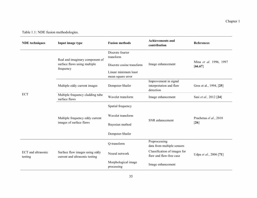
Chapter 1

35

Table 1.1: NDE fusion methodologies.

NDE techniques Input image type Fusion methods Achievements and

contribution References

ECT

Real and imaginary component of

surface flaws using multiple

frequency

Discrete fourier

transform

Image enhancement Mina et al. 1996, 1997

[66,67] Discrete cosine transform

Linear minimum least

mean square error

Multiple eddy current images Dempster­Shafer

Improvement in signal

interpretation and flaw

detection

Gros et al., 1994, [25]

Multiple frequency cladding tube

surface flaws Wavelet transform Image enhancement Sasi et al., 2012 [24]

Multiple frequency eddy current

images of surface flaws

Spatial frequency

SNR enhancement Prachetaa el al., 2010

[26]

Wavelet transform

Bayesian method

Dempster­Shafer

ECT and ultrasonic

testing

Surface flaw images using eddy

current and ultrasonic testing

Q­transform Preprocessing

data from multiple sensors

Udpa et al., 2006 [71] Neural network Classification of images for

flaw and flaw­free case

Morphological image

processing Image enhancement

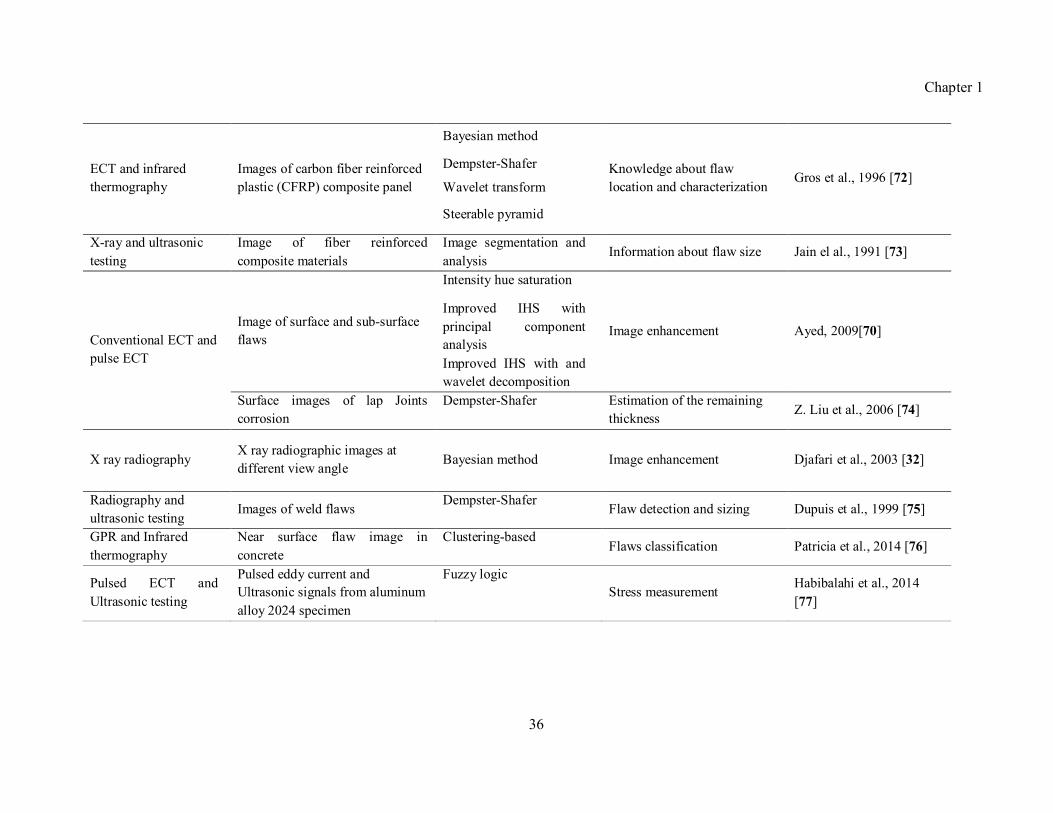
Chapter 1

36

ECT and infrared

thermography

Images of carbon fiber reinforced

plastic (CFRP) composite panel

Bayesian method

Knowledge about flaw

location and characterization Gros et al., 1996 [72]

Dempster­Shafer

Wavelet transform

Steerable pyramid

X­ray and ultrasonic

testing

Image of fiber reinforced

composite materials

Image segmentation and

analysis Information about flaw size Jain el al., 1991 [73]

Conventional ECT and

pulse ECT

Image of surface and sub­surface

flaws

Intensity hue saturation

Image enhancement Ayed, 2009[70]

Improved IHS with

principal component

analysis

Improved IHS with and

wavelet decomposition

Surface images of lap Joints

corrosion

Dempster­Shafer Estimation of the remaining

thickness Z. Liu et al., 2006 [74]

X ray radiography X ray radiographic images at

different view angle Bayesian method Image enhancement Djafari et al., 2003 [32]

Radiography and

ultrasonic testing Images of weld flaws

Dempster­Shafer Flaw detection and sizing Dupuis et al., 1999 [75]

GPR and Infrared

thermography

Near surface flaw image in

concrete

Clustering­based Flaws classification Patricia et al., 2014 [76]

Pulsed ECT and

Ultrasonic testing

Pulsed eddy current and

Ultrasonic signals from aluminum

alloy 2024 specimen

Fuzzy logic

Stress measurement Habibalahi et al., 2014

[77]

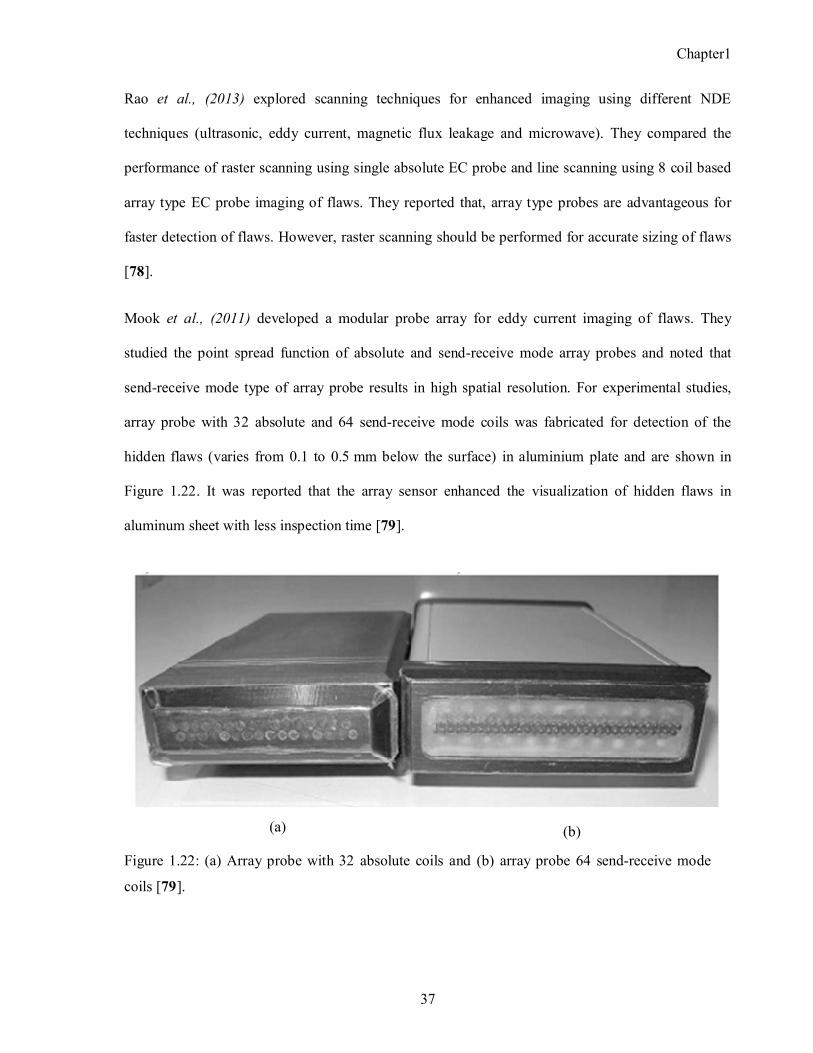
Chapter1

37

Rao et al., (2013) explored scanning techniques for enhanced imaging using different NDE

techniques (ultrasonic, eddy current, magnetic flux leakage and microwave). They compared the

performance of raster scanning using single absolute EC probe and line scanning using 8 coil based

array type EC probe imaging of flaws. They reported that, array type probes are advantageous for

faster detection of flaws. However, raster scanning should be performed for accurate sizing of flaws

[78].

Mook et al., (2011) developed a modular probe array for eddy current imaging of flaws. They

studied the point spread function of absolute and send­receive mode array probes and noted that

send­receive mode type of array probe results in high spatial resolution. For experimental studies,

array probe with 32 absolute and 64 send­receive mode coils was fabricated for detection of the

hidden flaws (varies from 0.1 to 0.5 mm below the surface) in aluminium plate and are shown in

Figure 1.22. It was reported that the array sensor enhanced the visualization of hidden flaws in

aluminum sheet with less inspection time [79].

Figure 1.22: (a) Array probe with 32 absolute coils and (b) array probe 64 send­receive mode

coils [79].

(a) (b)

Chapter1

38

Although there are a few advantages of using array type probes for imaging, there exist certain

drawbacks which limits their wide spread use. The drawbacks of the array probes are [80]:

1. Difficulty in manufacturing identical probes for effective imaging

2. Requirement of large number of probes to cover the scanning area

3. Lower sampling rate due to multiplexing

4. Software complexity for initial setup

5. Higher cost

This calls for the development of rapid scan plans to cover 100% surface area with less time using a

single EC probe without compromising the probability of detection and sizing accuracy. Hence, it is

attractive to study various scan plans using single coil probe for rapid and reliable imaging of flaws.

As raster scanning is time consuming to cover 100% surface area and tedious, studies have been

carried out by researchers to reduce the scanning time without compromising the probability of flaw

detection.

It is interesting to observe from literature that rapid detection and imaging of flaws is possible by

scanning with single EC probe using different scan plans followed in other imaging domains such as

microscopy, and astronomy [81,82,83,84].

Rao et al (2001) proposed an intelligent imaging scheme shown in Figure 1.23 using artificial neural

network for fast and automated detection, imaging and characterization of surface­flaws in 3.0 mm

thick stainless steel plates using a single coil probe. Binary images were obtained at coarse step size

of 1.0 mm and flaw region were localized and this localized region was subjected to fine scan with a

step size of 0.3 mm to obtain high resolution images by using separate artificial neural networks for

linear and circular flaws. Typical result of this intelligent imaging scheme is shown in Figure 1.24.

They reported an approximately ten­fold reduction in inspection time [85,23].

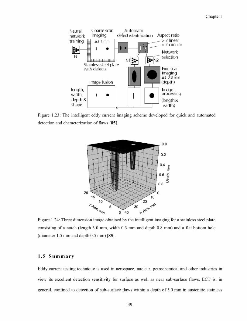
Chapter1

39

1.5 Summary

Eddy current testing technique is used in aerospace, nuclear, petrochemical and other industries in

view its excellent detection sensitivity for surface as well as near sub­surface flaws. ECT is, in

general, confined to detection of sub­surface flaws within a depth of 5.0 mm in austenitic stainless

Figure 1.24: Three dimension image obtained by the intelligent imaging for a stainless steel plate

consisting of a notch (length 3.0 mm, width 0.3 mm and depth 0.8 mm) and a flat bottom hole

(diameter 1.5 mm and depth 0.5 mm) [85].

Figure 1.23: The intelligent eddy current imaging scheme developed for quick and automated

detection and characterization of flaws [85].

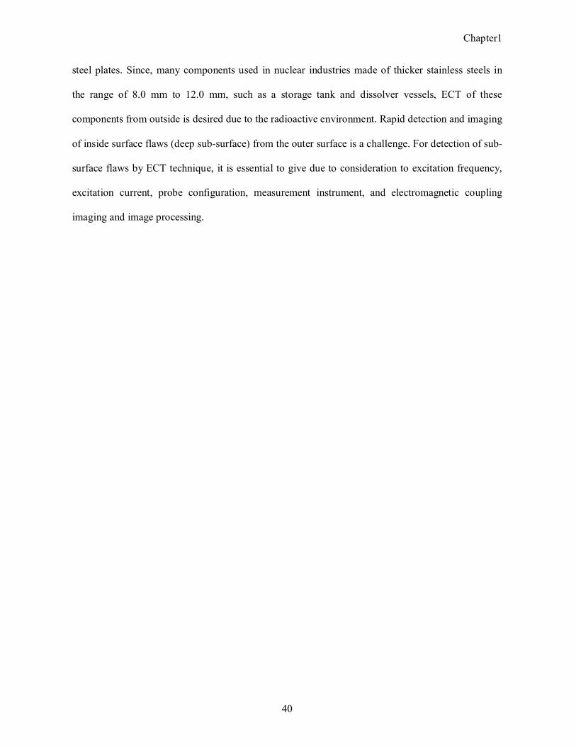
Chapter1

40

steel plates. Since, many components used in nuclear industries made of thicker stainless steels in

the range of 8.0 mm to 12.0 mm, such as a storage tank and dissolver vessels, ECT of these

components from outside is desired due to the radioactive environment. Rapid detection and imaging

of inside surface flaws (deep sub­surface) from the outer surface is a challenge. For detection of sub­

surface flaws by ECT technique, it is essential to give due to consideration to excitation frequency,

excitation current, probe configuration, measurement instrument, and electromagnetic coupling

imaging and image processing.

41

Motivation and Objective

2 .1 Preamble

This chapter identifies the gap areas based on the literature, which have helped in setting the

motivation and in identifying the objectives of the research work. This chapter also outlines the

organization of the thesis.

2.2 Motivat ion for re search

Austenitic stainless steel is one of the important core structural materials used in nuclear, chemical

and petrochemical industries. These steels are subjected to eddy current testing for quality

assessment and in­service inspection requirements. This technique is efficient in detecting surface as

well as near sub­surface flaws reliably. Due to the skin-effect, induced current density in the material

attenuates exponentially and this limits the sensitivity to detect flaws located upto 5.0 mm below the

surface. Detection of deep sub­surface flaws in austenitic stainless steels by ECT technique is

challenging. Research efforts towards enhancement of sensitivity to detect deep sub­surface flaws in

thick stainless steel plates using the ECT technique are worth focusing and exploring.

By changing the test parameters and conditions, the detection sensitivity of ECT technique can be

increased. The possible ways for enhancement of detection sensitivity are:

Increasing the depth of penetration (strengthening the primary magnetic field)

Development and use of high sensitive instrument and probes

Development and use of signal and image processing methodologies

2

Chapter 2

42

As observed from the literature, by using high throughput probes and using higher excitation current,

effective depth of penetration into stainless steel can be increased. Inspired by the encouraging

performance of the send­receive probe in the literature over the absolute probe, studies can be

focused on exploring the send­receive mode EC probes. It is also interesting to observe from the

literature that performance improvement of the EC probes is possible with the use of ferrite core and

shielding, especially send­receive type cup­core probes. In radioactive environments, the coil based

probe seems to be attractive for ECT of thick SS because solid state sensors undergo the radiation

damage. The existing literatures do not address detection of sub­surface flaws located beyond

5.0 mm in stainless steel components. Hence, there is strong need to optimize and design send­

receive type ferrite cored coil probes for detection of sub­surface flaws and corrosion damage in

austenitic stainless steel components.

Commercially available EC instruments have limitation for detection of flaws due to lower

excitation current levels and lack of precise measuring instruments for detection of feeble response

from sub­surface flaws. As observed from the literature, excitation current is important for

strengthening the primary field. Hence, development of a higher variable excitation current source

based excitation unit is attractive. To receive the feeble response from sub­surface flaws,

development of a high sensitive measurement system (of the order of �V) is essential. Although it is

known that phase measurement gives information about the depth of flaws, use of phase

measurement in ECT is very limited for sub­surface flaw detection. Hence, for detection of deep

sub­surface flaws in thick austenitic stainless steel development of a high power and high sensitive

precise phase measurement instrument is an attractive option.

EC imaging is essential for automated detection of flaws. EC images of large diameter probes suffer

from blurring due to the large foot print or point spread function (psf) of the EC probe. In this

context, it may be beneficial to adopt image processing techniques to improve the detection

sensitivity of sub­surface flaws. In the open literature, a variety of image processing methods viz.

Chapter 2

43

image denoising, filtering, pattern recognition, etc. have been reported. Inspired by the encouraging

performance of fusion of eddy current images in the literature, along with the recent developments in

the field of enhancement and denoising the EC images of surface flaws, studies can be focused on

exploring the image fusion methods for the enhancement of EC images of sub­surface flaws. The

image fusion methods reported in the literature, however, are limited to detection of surface flaws.

Details of image fusion methodologies for detection of sub­surface flaws in austenitic stainless steel

are not found in the open literature. Hence, development of image fusion methodologies can be

explored for detection of sub­surface flaws and improve the SNR.

For automated EC imaging of components for detection of flaws using a single sensor, raster scan

plan is used and it is time consuming. Alternative methods proposed in the literature use array

probes. Although, array probes are preferred for faster imaging, they require multi­channel systems

and data acquisition modules and are expensive. For detection and imaging of the flaws fast

scanning using single probe is still attractive. Development of efficient alternate fast scan plans to

reduce the time required for EC imaging without compromising the flaw detection performance is

worth exploring, specifically to use in radioactive conditions.

2.3 Object ive of research

The primary objective of the thesis is detection of deep sub­surface flaws in thick austenitic stainless

steel plates. Based on the inputs gained from the literature, the following objectives have been

arrived for automated rapid detection of deep sub­surface flaws:

1. To design and develop a high throughput eddy current coil based probe for detection of deep

sub­surface flaws in thick AISI 304L austenitic stainless steel plates (thickness of 12.0 mm).

2. To develop high sensitive eddy current instrument for detection of deep sub­surface flaws.

Chapter 2

44

3. To develop image fusion methodologies for improvement of SNR and probability of detection

of surface as well as deep sub­surface flaws and study the comparative performance of different

image fusion methods towards selection of an optimal methodology.

4. To explore possible alternative fast scan plans for a single coil based probe for rapid and

automated detection and imaging of sub­surface as well as surface flaws.

2.4 Organization o f the thesis

The thesis has been organized in four major chapters addressing the set objectives, towards

establishing methodologies for detection of sub­surface flaws in austenitic stainless steels, as given

below:

Chapter 3 presents the finite element model based probe optimisation methodology for designing a

high throughput probe for detection of sub­surface flaws. For this study, four possible different

probe configurations have been analysed for selection of the optimum configuration. This chapter

also discusses a study on the dimensions of the optimum probe configuration and frequency

selection.

Chapter 4 explains the design and development of a high sensitive eddy current instrument for

detection of sub­surface flaws. This chapter also discusses the performance assessment of the

developed EC instrument for detection of sub­surface as well as surface flaws in 12.0 mm thick

austenitic stainless steel plates.

Chapter 5 discusses the development of a novel image fusion methodology for enhanced detection of

sub­surface flaws. The comparison of the proposed image fusion methodology with existing image

fusion methodologies in ECT based on the different quality assessment parameters is undertaken in

this chapter.

Chapter 2

45

Chapter 6 explains the importance of rapid detection and imaging of flaws in ECT. This chapter

presents the simulation results of different scan plans and compares their performance with the

conventional raster scan plan. This chapter also discusses the experimental investigations carried out

to study the influence of flaw dimensions and scan step size on flaw detection.

Chapter 7 summarises the major conclusions drawn from the research work and provides the scope

for future research.

46

Design and development of eddy current

probe

3 .1 Preamble

The scope of this chapter is to study the design optimisation of eddy current probes for detection

of deep sub­surface flaws in thick austenitic stainless steel plates. The chapter discusses different

types of send­receive type probe viz. air core, ferrite core, ferrite core with outer shielding and

cup­core probes and comparison of performance of these probes using model predicted

parameters viz., magnetic flux density, eddy current density and change in phase angle.

Subsequently, for detection of sub­surface flaws, selection of optimum probe diameter and

excitation frequency is discussed in this chapter.

For detection of deep sub­surface flaws, optimisation of probe configuration that strengthens the

primary magnetic field for higher penetration into the material is essential. Practically,

fabrication of different types of probes for selection of optimum probe by experimentation is

time consuming and expensive. In view of this, finite element (FE) modelling is used in this

study.

3.2 Finite element modell ing

FE modelling was first proposed in the 1940s [86] and its use began in the 1960s for structural

and continuum mechanics and later found a wide variety of applications in electromagnetic field

problems [87]. Subsequently, FE Modelling has also been exploited well by NDE research

community [10,88,89]. Today, the FE Modelling has become a powerful tool for designing eddy

current probes for varied test situations.

3

Chapter 3

47

In a FE model, the governing partial differential equation is solved in the problem domain. The

problem domain is discretised into a number of composite sub­domain called elements which

make up a mesh. In 2D axi­symmetry models triangular elements are widely used. The

interconnecting points of elements are called nodes. The exact variation of the unknown function

(e.g. potential) is approximated by a simple interpolation functions with unknown coefficients at

each nodes associated with the elements. In other words, the original boundary value problem

with infinite degrees of freedom is transformed into a problem with finite degrees of freedom.

Then, a system of algebraic equations is obtained by applying the Ritz variational or Galerkin

procedure and solution of the boundary value problem is obtained by solving the system of

equations. Finally, the desired parameters such as potential, field, current density etc. are

computed at the nodes situated within the region of interest [10,90].

For FE model based optimisation of eddy current probe configuration, COMSOL multi­physics

4.4 software is used in 2D axi­symmetry environment. State­of­the­art solvers are embedded in

the package for the user to address complicated problems quickly and accurately [91]. For

numerical simulation of model in COMSOL, suitable governing partial differential equations are

formed and used.

3.3 Governing equations for eddy current test ing

The governing partial differential equation of the ECT technique is derived from the Maxwell’s

equations given below [7,10,86]

∇ × � = − ��

�� (3.1)

∇ × � = � +��

�� (3.2)

∇. � = 0 (3.3)

Chapter 3

48

∇. � = 0 (3.4)

where E is electric field, B is magnetic flux density, H is magnetic field intensity, J is current

density and D is the displacement current. In equation 3.2 the displacement current term can

be ignored as it is insignificant in quasi static cases (equation 3.4). From the equation 3.3 the

divergence of B is zero, so B can be expressed as the curl of another vector called the

magnetic vector potential, A defined as:

B = ∇ × � (3.5)

The governing partial differential equation which is used for solution of eddy current FE

model is derived by using Maxwell’s equations and the constitutive relation � = ��

and � = �� and given as:

∇ × (∇ × �) = �σ�� − σ∇V + �� (3.6)

where V is the electric scalar potential, σ is the electrical conductivity, μ is magnetic

permeability, ω is angular frequency of the sinusoidal excitation and Js is the applied source

current density.

3.4 Finite element model for eddy current te sting

In COMSOL software by using the 2D axi­symmetry model, solution will be fast and accurate as

finer mesh density is possible and propagation errors are less. Therefore, for the chosen EC

probe type with cylindrical symmetry, 2D axi­symmetry model is selected for optimization of

the EC probe configuration and dimension. The FE modelling steps involved using COMSOL

are discussed in this section.

3.4.1 Construction of model geometry

In 2D axi­symmetry models a quarter of the problem domain is projected onto a 2D plane.

Modelled geometry consists of EC probe and austenitic stainless steel plate enclosed in an

Chapter 3

49

outer boundary. The model is truncated into a finite region by defining an external boundary

model which limits the solutions to be calculated inside the assigned region. Drichlet

boundary condition (A=0) has been applied at the line of symmetry and at the outer

boundary. Table 3.1 gives the details of sub­domain parameters values i.e. µ and σ used in the

model. The conductivity of air sub­domain is set to a non­zero value to avoid computational

problems typically encountered during FE solution, when dependent variable vanishes [92].

The typical geometry of model with a boundary region is shown in Figure 3.1

Table 3.1: Details of the sub­domain parameters used in the FE model.

S. No. Material Conductivity (σ), S/m Relative magnetic

permeability (µr)

1. Air 10 1

2. Copper 5.88× 107 1

3. Ferrite 100 1500

4. Stainless steel 1.38×106 1

Figure 3.1: The typical geometry of model with a boundary region.

Chapter 3

50

3.4.2 Meshing

In the model geometry, the region of interest is divided into a mesh of triangular­shaped

elements. Higher accuracy is obtained by the generation of a fine mesh within the region of

interest. SS plate with flaws and EC coil are the important regions to visualise the field

distribution and hence, these regions are set at a more refined mesh. In the modelled

geometry a total of 154378 triangular elements have been generated. 44 mesh layers have

been chosen along the material thickness of 12.0 mm. This enhances the mesh quality around

the flaw and the surrounding region where the direction or the magnitude of the magnetic

field changes rapidly. Figure 3.2 shows discritisation of the mesh.

3.4.3 Equation solving

The generated geometry is solved by using the governing partial differential equation 3.6.

This governing equation is complex and symmetric in nature. Hence, the complex symmetric

version of the Multifrontal Massively Parallel sparse direct Solver (MUMPS) is used.

MUMPS ensures faster computation with minimal storage. For solving a typical problem

Figure 3.2: Discritisation of triangular mesh in the modelled geometry.

Chapter 3

51

having 154378 degrees of freedom, 8s time is required by the solver in work station

(configuration are Pentium 4, 1.6 Ghz clock speed and 8 GB RAM).

3.4.4 Post-processing

Post processing is performed to calculate the magnetic flux density, induced current density,

induced voltage in coil from the model predicted vector potential data [10]. The typical surface

plot of magnetic flux density (B) with contour of induced current density (Je) is shown in Figure

3.3. Data from the plots can be used for detailed analysis and understanding the field­flaw

interactions.

3.5 Model based optimisa tion of probe configuration

As discussed in Section 1.3.3 and Section 1.4.1, a variety of probe configurations like absolute

probe, differential probe, send­receive probe etc. are commonly used and optimisation of probe

configuration is important. In this regard, send­receive type EC probes of different

configurations viz. air core, ferrite core, ferrite core with outer shielding and cup­core have been

Figure 3.3: Typical surface and contour plot of magnetic flux density and induced current

density.

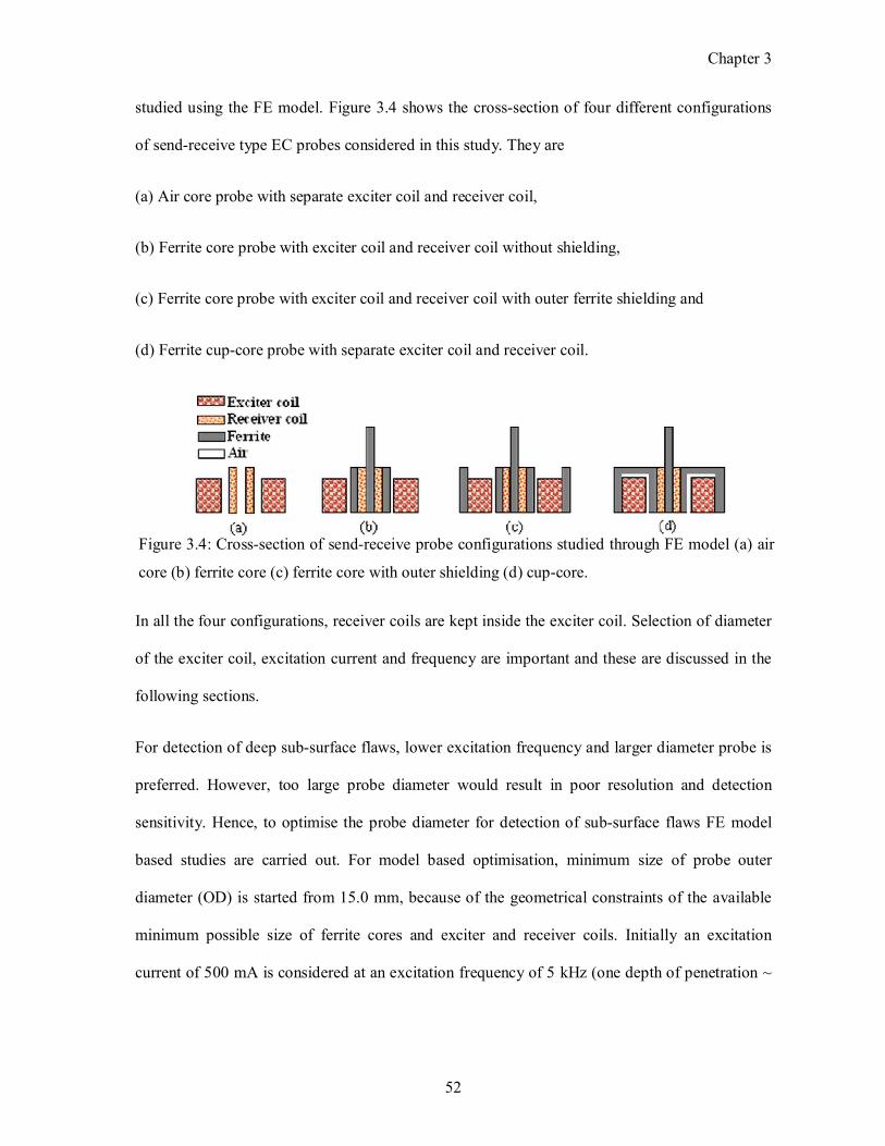
Chapter 3

52

studied using the FE model. Figure 3.4 shows the cross­section of four different configurations

of send­receive type EC probes considered in this study. They are

(a) Air core probe with separate exciter coil and receiver coil,

(b) Ferrite core probe with exciter coil and receiver coil without shielding,

(c) Ferrite core probe with exciter coil and receiver coil with outer ferrite shielding and

(d) Ferrite cup­core probe with separate exciter coil and receiver coil.

In all the four configurations, receiver coils are kept inside the exciter coil. Selection of diameter

of the exciter coil, excitation current and frequency are important and these are discussed in the

following sections.

For detection of deep sub­surface flaws, lower excitation frequency and larger diameter probe is

preferred. However, too large probe diameter would result in poor resolution and detection

sensitivity. Hence, to optimise the probe diameter for detection of sub­surface flaws FE model

based studies are carried out. For model based optimisation, minimum size of probe outer

diameter (OD) is started from 15.0 mm, because of the geometrical constraints of the available

minimum possible size of ferrite cores and exciter and receiver coils. Initially an excitation

current of 500 mA is considered at an excitation frequency of 5 kHz (one depth of penetration ~

Figure 3.4: Cross­section of send­receive probe configurations studied through FE model (a) air

core (b) ferrite core (c) ferrite core with outer shielding (d) cup­core.

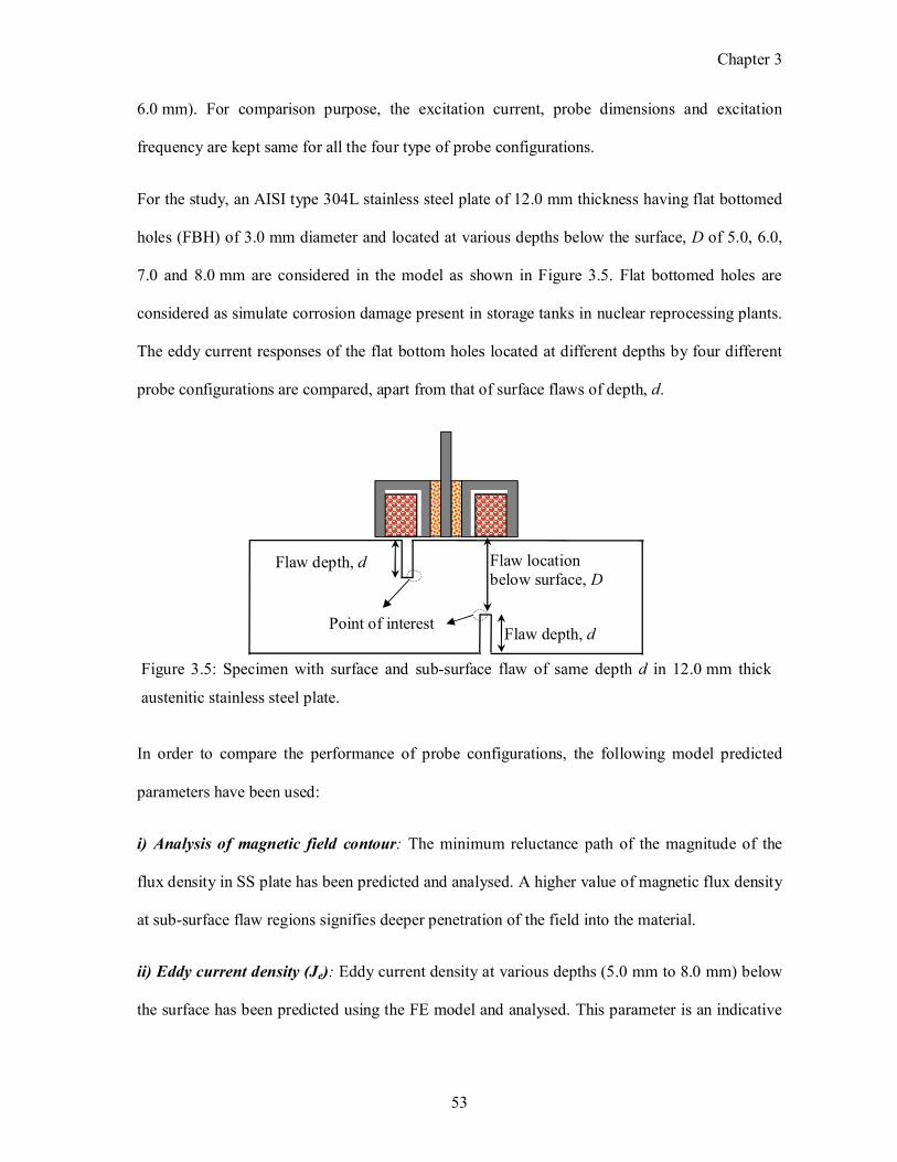
Chapter 3

53

6.0 mm). For comparison purpose, the excitation current, probe dimensions and excitation

frequency are kept same for all the four type of probe configurations.

For the study, an AISI type 304L stainless steel plate of 12.0 mm thickness having flat bottomed

holes (FBH) of 3.0 mm diameter and located at various depths below the surface, D of 5.0, 6.0,

7.0 and 8.0 mm are considered in the model as shown in Figure 3.5. Flat bottomed holes are

considered as simulate corrosion damage present in storage tanks in nuclear reprocessing plants.

The eddy current responses of the flat bottom holes located at different depths by four different

probe configurations are compared, apart from that of surface flaws of depth, d.

In order to compare the performance of probe configurations, the following model predicted

parameters have been used:

i) Analysis of magnetic field contour: The minimum reluctance path of the magnitude of the

flux density in SS plate has been predicted and analysed. A higher value of magnetic flux density

at sub­surface flaw regions signifies deeper penetration of the field into the material.

ii) Eddy current density (Je): Eddy current density at various depths (5.0 mm to 8.0 mm) below

the surface has been predicted using the FE model and analysed. This parameter is an indicative

Point of interest

Flaw depth, d Flaw location below surface, D

Flaw depth, d

Figure 3.5: Specimen with surface and sub­surface flaw of same depth d in 12.0 mm thick

austenitic stainless steel plate.

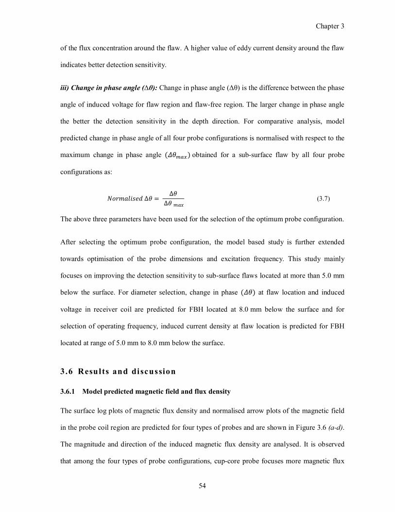
Chapter 3

54

of the flux concentration around the flaw. A higher value of eddy current density around the flaw

indicates better detection sensitivity.

iii) Change in phase angle (∆θ): Change in phase angle (Δθ) is the difference between the phase

angle of induced voltage for flaw region and flaw­free region. The larger change in phase angle

the better the detection sensitivity in the depth direction. For comparative analysis, model

predicted change in phase angle of all four probe configurations is normalised with respect to the

maximum change in phase angle (�����) obtained for a sub­surface flaw by all four probe

configurations as:

���������� ∆� = ∆�

∆� ��� (3.7)

The above three parameters have been used for the selection of the optimum probe configuration.

After selecting the optimum probe configuration, the model based study is further extended

towards optimisation of the probe dimensions and excitation frequency. This study mainly

focuses on improving the detection sensitivity to sub­surface flaws located at more than 5.0 mm

below the surface. For diameter selection, change in phase (��) at flaw location and induced

voltage in receiver coil are predicted for FBH located at 8.0 mm below the surface and for

selection of operating frequency, induced current density at flaw location is predicted for FBH

located at range of 5.0 mm to 8.0 mm below the surface.

3.6 Results and discussion

3.6.1 Model predicted magnetic field and flux density

The surface log plots of magnetic flux density and normalised arrow plots of the magnetic field

in the probe coil region are predicted for four types of probes and are shown in Figure 3.6 (a-d).

The magnitude and direction of the induced magnetic flux density are analysed. It is observed

that among the four types of probe configurations, cup­core probe focuses more magnetic flux

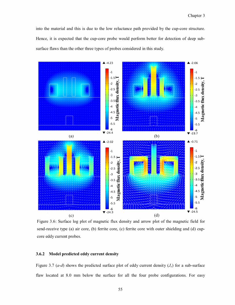
Chapter 3

55

into the material and this is due to the low reluctance path provided by the cup­core structure.

Hence, it is expected that the cup­core probe would perform better for detection of deep sub­

surface flaws than the other three types of probes considered in this study.

3.6.2 Model predicted eddy current density

Figure 3.7 (a-d) shows the predicted surface plot of eddy current density (Je) for a sub­surface

flaw located at 8.0 mm below the surface for all the four probe configurations. For easy

Figure 3.6: Surface log plot of magnetic flux density and arrow plot of the magnetic field for

send­receive type (a) air core, (b) ferrite core, (c) ferrite core with outer shielding and (d) cup­

core eddy current probes.

(c)

(b) (a)

(d)

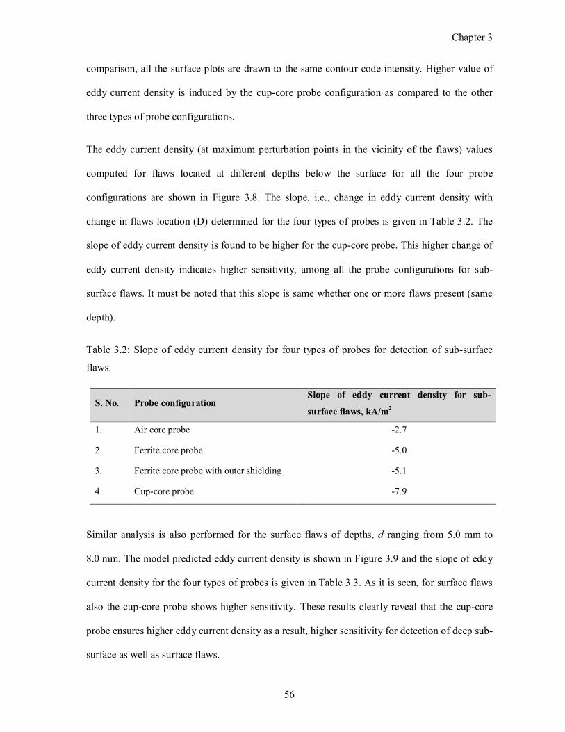
Chapter 3

56

comparison, all the surface plots are drawn to the same contour code intensity. Higher value of

eddy current density is induced by the cup­core probe configuration as compared to the other

three types of probe configurations.

The eddy current density (at maximum perturbation points in the vicinity of the flaws) values

computed for flaws located at different depths below the surface for all the four probe

configurations are shown in Figure 3.8. The slope, i.e., change in eddy current density with

change in flaws location (D) determined for the four types of probes is given in Table 3.2. The

slope of eddy current density is found to be higher for the cup­core probe. This higher change of

eddy current density indicates higher sensitivity, among all the probe configurations for sub­

surface flaws. It must be noted that this slope is same whether one or more flaws present (same

depth).

Table 3.2: Slope of eddy current density for four types of probes for detection of sub­surface

flaws.

S. No. Probe configuration Slope of eddy current density for sub-

surface flaws, kA/m2

1. Air core probe ­2.7

2. Ferrite core probe ­5.0

3. Ferrite core probe with outer shielding ­5.1

4. Cup­core probe ­7.9

Similar analysis is also performed for the surface flaws of depths, d ranging from 5.0 mm to

8.0 mm. The model predicted eddy current density is shown in Figure 3.9 and the slope of eddy

current density for the four types of probes is given in Table 3.3. As it is seen, for surface flaws

also the cup­core probe shows higher sensitivity. These results clearly reveal that the cup­core

probe ensures higher eddy current density as a result, higher sensitivity for detection of deep sub­

surface as well as surface flaws.

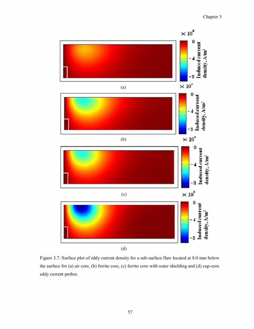
Chapter 3

57

(a)

(c)

(b)

(d)

Figure 3.7: Surface plot of eddy current density for a sub­surface flaw located at 8.0 mm below

the surface for (a) air core, (b) ferrite core, (c) ferrite core with outer shielding and (d) cup­core

eddy current probes.

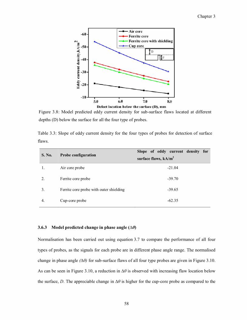
Chapter 3

58

Table 3.3: Slope of eddy current density for the four types of probes for detection of surface

flaws.

S. No. Probe configuration Slope of eddy current density for

surface flaws, kA/m2

1. Air core probe ­21.04

2. Ferrite core probe ­39.70

3. Ferrite core probe with outer shielding ­39.65

4. Cup­core probe ­62.35

3.6.3 Model predicted change in phase angle (∆θ)

Normalisation has been carried out using equation 3.7 to compare the performance of all four

types of probes, as the signals for each probe are in different phase angle range. The normalised

change in phase angle (∆θ) for sub­surface flaws of all four type probes are given in Figure 3.10.

As can be seen in Figure 3.10, a reduction in ∆θ is observed with increasing flaw location below

the surface, D. The appreciable change in ∆θ is higher for the cup­core probe as compared to the

Figure 3.8: Model predicted eddy current density for sub­surface flaws located at different

depths (D) below the surface for all the four type of probes.

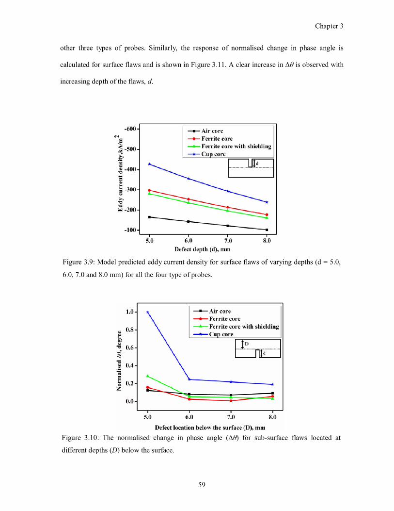
Chapter 3

59

other three types of probes. Similarly, the response of normalised change in phase angle is

calculated for surface flaws and is shown in Figure 3.11. A clear increase in ∆θ is observed with

increasing depth of the flaws, d.

Figure 3.10: The normalised change in phase angle (∆θ) for sub­surface flaws located at

different depths (D) below the surface.

Figure 3.9: Model predicted eddy current density for surface flaws of varying depths (d = 5.0,

6.0, 7.0 and 8.0 mm) for all the four type of probes.

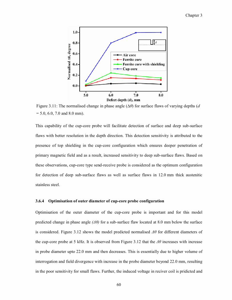
Chapter 3

60

This capability of the cup­core probe will facilitate detection of surface and deep sub­surface

flaws with better resolution in the depth direction. This detection sensitivity is attributed to the

presence of top shielding in the cup­core configuration which ensures deeper penetration of

primary magnetic field and as a result, increased sensitivity to deep sub­surface flaws. Based on

these observations, cup­core type send­receive probe is considered as the optimum configuration

for detection of deep sub­surface flaws as well as surface flaws in 12.0 mm thick austenitic

stainless steel.

3.6.4 Optimisation of outer diameter of cup-core probe configuration

Optimisation of the outer diameter of the cup­core probe is important and for this model

predicted change in phase angle (Δθ) for a sub­surface flaw located at 8.0 mm below the surface

is considered. Figure 3.12 shows the model predicted normalised Δθ for different diameters of

the cup­core probe at 5 kHz. It is observed from Figure 3.12 that the Δθ increases with increase

in probe diameter upto 22.0 mm and then decreases. This is essentially due to higher volume of

interrogation and field divergence with increase in the probe diameter beyond 22.0 mm, resulting

in the poor sensitivity for small flaws. Further, the induced voltage in reciver coil is pridicted and

Figure 3.11: The normalised change in phase angle (∆θ) for surface flaws of varying depths (d

= 5.0, 6.0, 7.0 and 8.0 mm).

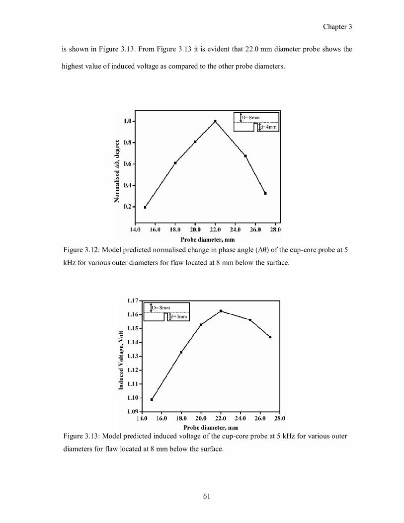
Chapter 3

61

is shown in Figure 3.13. From Figure 3.13 it is evident that 22.0 mm diameter probe shows the

highest value of induced voltage as compared to the other probe diameters.

Figure 3.13: Model predicted induced voltage of the cup­core probe at 5 kHz for various outer

diameters for flaw located at 8 mm below the surface.

Figure 3.12: Model predicted normalised change in phase angle (Δθ) of the cup­core probe at 5

kHz for various outer diameters for flaw located at 8 mm below the surface.

Chapter 3

62

In order to verify the performance of 22.0 mm optimised probe diameter, magnetic flux density,

eddy current density and change in phase angle for 22.0 mm diameter have been pridicted and

shown in Figure 3.14. The results have compared with that of the 15.0 mm diameter probes and

no changes in trends (Figure 3.8 to Figure 3.11) have been observed. However, the 22.0 mm

diameter probes resultes have better detection sensitivity as compared to 15.0 mm diameter

probes. Hence, the cup­core probe of 22.0 mm diameter is selected as the optimum for detection

of deep sub­surface flaws in 12.0 mm thick SS plates and this is fabricated for experimental

studies.

3.6.5 Selection of excitation frequency of cup-core probe

The performance of the optimised cup­core probe at different excitation frequencies is studied

based on induced current density at flaw region. For this study, frequencies of 3 kHz, 5 kHz and

7 kHz are chosen. The induced current density at different depths ranging from 5.0 mm to 8.0

mm below surface in the specimen is predicted at 3 kHz, 5 kHz and 7 kHz and the result are

shown in Figure 3.15. From the Figure 3.15, it is clearly seen that the induced current density of

a sub­surface flaw located at 5.0 mm to 8.0 mm depths is higher for the excitation frequency of

5 kHz as compared to that of at 3 kHz and 7 kHz. It is also observed that the over all change in

induced current density as function of flaw depth is higher at 7 kHz and at 3 kHz the change in

induced current desity is lower. However, the change in the induced current density and the

amplitude of induced current density at 7.0 mm and 8.0 mm at 7 kHz is lower than that of at

5 kHz. The higher value of induced current density at 5 kHz is responsible for enhanced

detection sensitivity. Hence, frequency 5 kHz is selected as the suitable frequency for detection

of sub­surface flaws as it shows higher induced current density as well as higher change in

induced current density as a function of the flaw depth below the surface.

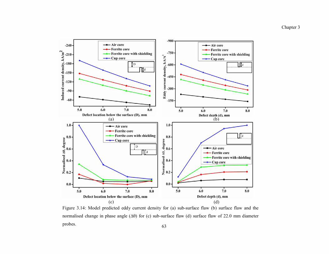
Chapter 3

63

(a) (b)

(d) (c)

Figure 3.14: Model predicted eddy current density for (a) sub­surface flaw (b) surface flaw and the

normalised change in phase angle (∆θ) for (c) sub­surface flaw (d) surface flaw of 22.0 mm diameter

probes.

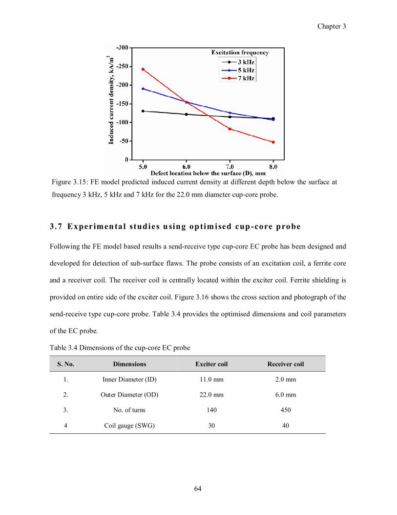
Chapter 3

64

3.7 Experimental studies using optimised cup-core probe

Following the FE model based results a send­receive type cup­core EC probe has been designed and

developed for detection of sub­surface flaws. The probe consists of an excitation coil, a ferrite core

and a receiver coil. The receiver coil is centrally located within the exciter coil. Ferrite shielding is

provided on entire side of the exciter coil. Figure 3.16 shows the cross section and photograph of the

send­receive type cup­core probe. Table 3.4 provides the optimised dimensions and coil parameters

of the EC probe.

Table 3.4 Dimensions of the cup­core EC probe

S. No. Dimensions Exciter coil Receiver coil

1. Inner Diameter (ID) 11.0 mm 2.0 mm

2. Outer Diameter (OD) 22.0 mm 6.0 mm

3. No. of turns 140 450

4 Coil gauge (SWG) 30 40

Figure 3.15: FE model predicted induced current density at different depth below the surface at

frequency 3 kHz, 5 kHz and 7 kHz for the 22.0 mm diameter cup­core probe.

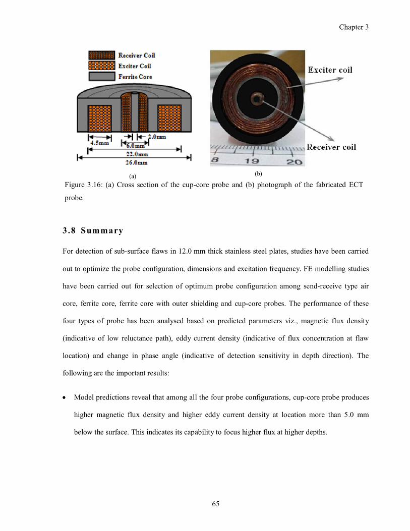
Chapter 3

65

3.8 Summary

For detection of sub­surface flaws in 12.0 mm thick stainless steel plates, studies have been carried

out to optimize the probe configuration, dimensions and excitation frequency. FE modelling studies

have been carried out for selection of optimum probe configuration among send­receive type air

core, ferrite core, ferrite core with outer shielding and cup­core probes. The performance of these

four types of probe has been analysed based on predicted parameters viz., magnetic flux density

(indicative of low reluctance path), eddy current density (indicative of flux concentration at flaw

location) and change in phase angle (indicative of detection sensitivity in depth direction). The

following are the important results:

Model predictions reveal that among all the four probe configurations, cup­core probe produces

higher magnetic flux density and higher eddy current density at location more than 5.0 mm

below the surface. This indicates its capability to focus higher flux at higher depths.

(a) (b)

Figure 3.16: (a) Cross section of the cup­core probe and (b) photograph of the fabricated ECT

probe.

Chapter 3

66

The change in phase angle for flaws located at various depths is higher for the cup­core probe as

compared to that of the air core, ferrite core and ferrite core probes with outer shielding. This

promises better detection sensitivity in the depth direction by cup­core probe.

For selection of optimum cup­core probe diameter for 12.0 mm thick stainless steel plate change

in phase angle at flaw location and induced voltage in receiver coil have been predicted using the

FE model for the first time. The cup­core probe of 22.0 mm outer diameter has shown larger

change in phase angle as well as the magnitude of induced voltage. Hence, this probe is selected

for detection of sub­surface flaws.

The induced current density at different depths has been predicted for the cup­core probe at

3 kHz, 5 kHz and 7 kHz. Higher response for sub­surface flaws located at ranges of 5.0 mm to

8.0 mm below the surface has been observed at 5 kHz. Send­receive type cup­core probe has

been fabricated for experimental studies on detection of sub­surface flaws.

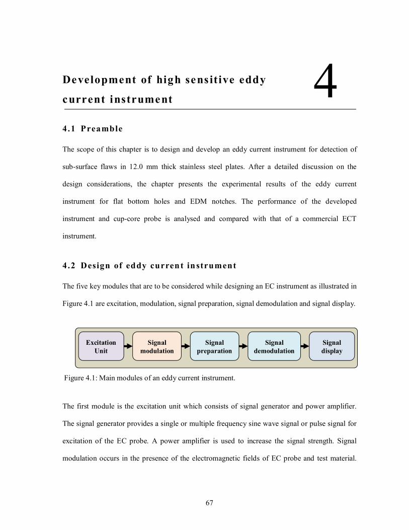
67

Development of high sens itive eddy

current instrument

4.1 Preamble

The scope of this chapter is to design and develop an eddy current instrument for detection of

sub­surface flaws in 12.0 mm thick stainless steel plates. After a detailed discussion on the

design considerations, the chapter presents the experimental results of the eddy current

instrument for flat bottom holes and EDM notches. The performance of the developed

instrument and cup­core probe is analysed and compared with that of a commercial ECT

instrument.

4.2 Design of eddy current instrument

The five key modules that are to be considered while designing an EC instrument as illustrated in

Figure 4.1 are excitation, modulation, signal preparation, signal demodulation and signal display.

The first module is the excitation unit which consists of signal generator and power amplifier.

The signal generator provides a single or multiple frequency sine wave signal or pulse signal for

excitation of the EC probe. A power amplifier is used to increase the signal strength. Signal

modulation occurs in the presence of the electromagnetic fields of EC probe and test material.

Signal

modulation Signal

preparation Signal

demodulation Signal display

Excitation Unit

Figure 4.1: Main modules of an eddy current instrument.

4

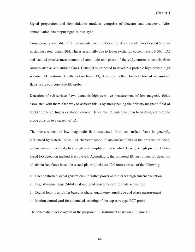
Chapter 4

68

Signal preparation and demodulation modules comprise of detector and analyzers. After

demodulation, the output signal is displayed.

Commercially available ECT instruments have limitation for detection of flaws beyond 5.0 mm

in stainless steel plates [56]. This is essentially due to lower excitation current levels (<300 mA)

and lack of precise measurement of amplitude and phase of the eddy current sinusoids from

sources such as sub­surface flaws. Hence, it is proposed to develop a portable high­power, high

sensitive EC instrument with lock­in based I/Q detection method for detection of sub­surface

flaws using cup­core type EC probe.

Detection of sub­surface flaws demands high sensitive measurement of low magnetic fields

associated with them. One way to achieve this is by strengthening the primary magnetic field of

the EC probe i.e. higher excitation current. Hence, the EC instrument has been designed to excite

probe coils up to a current of 1A.

The measurement of low magnitude field associated from sub­surface flaws is generally

influenced by material noise. For characterization of sub­surface flaws in the presence of noise,

precise measurement of phase angle and amplitude is essential. Hence, a high precise lock­in

based I/Q detection method is employed. Accordingly, the proposed EC instrument for detection

of sub­surface flaws in stainless steel plates (thickness 12.0 mm) consists of the following:

1. User controlled signal generation unit with a power amplifier for high current excitation

2. High dynamic range 24­bit analog­digital converter card for data acquisition

3. Digital lock­in amplifier based in­phase, quadrature, amplitude and phase measurement

4. Motion control card for automated scanning of the cup­core type ECT probe

The schematic block diagram of the proposed EC instrument is shown in Figure 4.2.

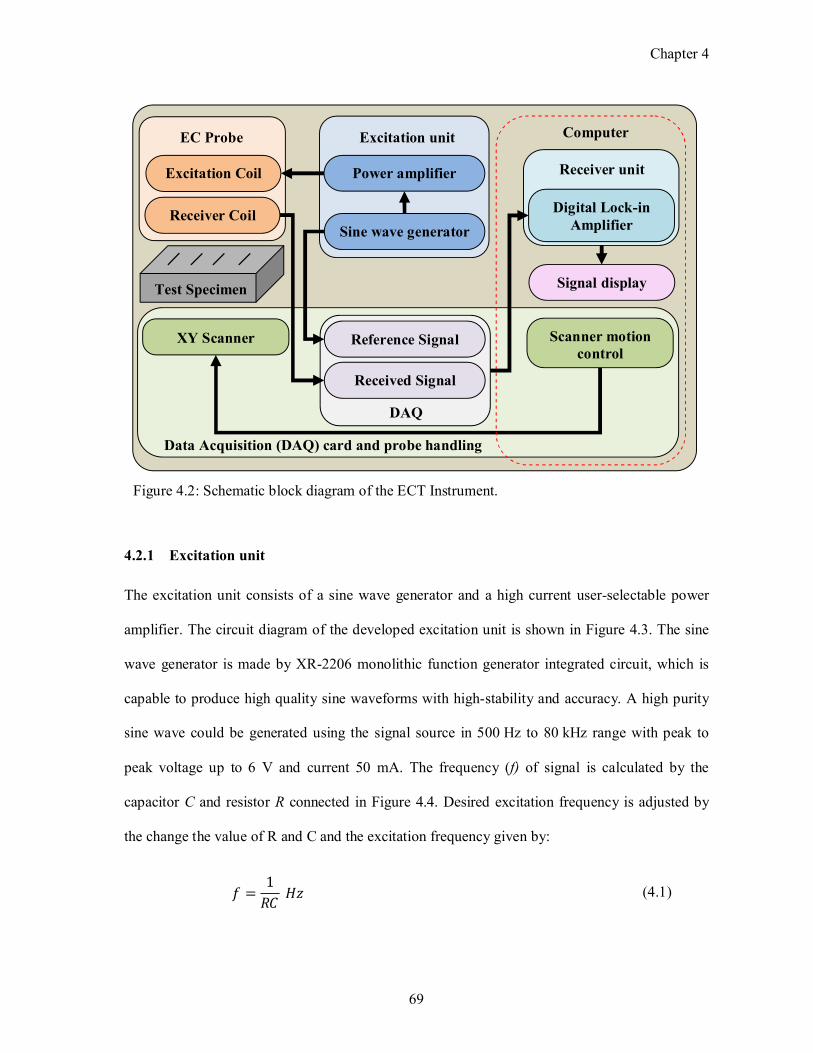
Chapter 4

69

4.2.1 Excitation unit

The excitation unit consists of a sine wave generator and a high current user­selectable power

amplifier. The circuit diagram of the developed excitation unit is shown in Figure 4.3. The sine

wave generator is made by XR­2206 monolithic function generator integrated circuit, which is

capable to produce high quality sine waveforms with high­stability and accuracy. A high purity

sine wave could be generated using the signal source in 500 Hz to 80 kHz range with peak to

peak voltage up to 6 V and current 50 mA. The frequency (f) of signal is calculated by the

capacitor C and resistor R connected in Figure 4.4. Desired excitation frequency is adjusted by

the change the value of R and C and the excitation frequency given by:

� =1

�� �� (4.1)

Excitation Coil

Receiver Coil

EC Probe

XY Scanner

Test Specimen

Sine wave generator

Power amplifier

Reference Signal

Received Signal

Computer

Signal display

Scanner motion control

Data Acquisition (DAQ) card and probe handling

Excitation unit

Digital Lock-in Amplifier

Receiver unit

DAQ

Figure 4.2: Schematic block diagram of the ECT Instrument.

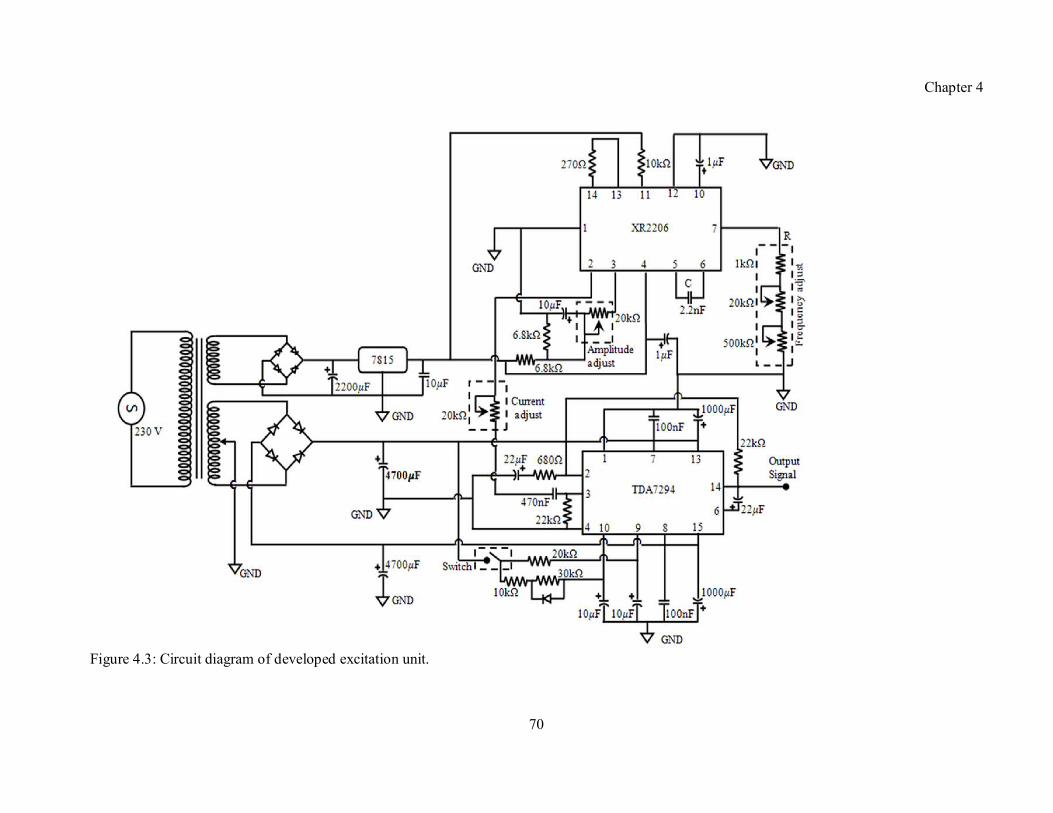
Chapter 4

70

Figure 4.3: Circuit diagram of developed excitation unit.

Chapter 4

71

The power amplifier used in the excitation unit is made by the TDA7294 monolithic integrated

circuit. In the power amplifier, mixed bipolar­MOS and high­power DMOS buffer is used for

handling the extremely high current and voltage levels while maintaining acceptably low

harmonic distortion and good behavior over frequency response. The output voltage of the power

amplifier is made variable by the voltage divided rule to change the excitation current. By this

way, a sine wave signal of output current upto 1 A is obtained with low harmonic distortion and

excellent frequency response

The signal generator and amplifier circuits are tested for stability, distortion, higher current and

harmonic content free sine waves. In order to assess the purity of the sine wave, the total

harmonic distortion (THD) has been measured. THD is defined as the ratio of the sum of the

powers of all harmonic components to the power of the fundamental frequency as shown in the

equation given below:

��� % = �� + �� + �� + ⋯ … + ��

�� × 100 (4.2)

The powers of the harmonic components of the waveform have been evaluated by computing the

power spectral density using the fast Fourier transform. The sine wave after the power amplifier

has been found to be pure with a THD of less than 1%, when the source has not been connected

to any load. The THD has been found to be less than 2.5% when it is connected to a 50 Ω

inductive load at an excitation frequency of 5 kHz.

4.2.2 Reception unit

EC probe signals are influenced by noise from various sources i.e material surface, instrument,

environment etc. The induced eddy currents are attenuated with depth. Because of this, the

amplitude of the received EC signal from sub­surface flaws is feeble. The detected signals are

also influenced by the variations in material properties such as the permeability, surface

Chapter 4

72

roughness and lift­off that produce high frequency noise. Hence, for extraction of the

information from sub­surface flaws, a high sensitive precise phase measurement unit based on

lock­in amplifier has been developed.

A digital lock­in amplifier has been implemented for measurement of in­phase, quadrature,

magnitude and phase angle. The digital lock­in amplifier measures the phase and magnitude of

the receiver coil sinusoid (input sine wave) with respect to reference sinusoid of the exciter coil.

It locks the frequency of the sinusoids that matches the reference frequency, thereby acting as a

narrow band pass filter with a bandwidth of the order of mHz.

A schematic working of the lock­in amplifier is shown in Figure 4.4. In this, the magnitude ‘A’

and the phase angle ‘θ’ of an input sine wave of angular frequency ωs, are measured with respect

to a reference sine wave of angular frequency ωR. The phase locked loop (PLL) block measures

the frequency of the reference sine wave and generates orthogonal sine and cosine components.

These two waves are individually multiplied with the input sine wave. The resulting components

have additive and subtractive frequency terms in sine and cosine as shown in Figure 4.4. When

there is a match between the reference frequency and the input sine wave frequency, the additive

terms give the higher frequency components (ω) and the subtractive terms provide the DC

components. The higher frequency components are filtered using a low­pass filter to obtain the

DC components X and Y which are respectively the in­phase (X) and quadrature (Y)

components of the receiver coil induced voltage. The magnitude (A) and the phase angle (θ) are

calculated from the measured in­phase and quadrature components. This digital lock­in amplifier

has been implemented in LabVIEW environment. In the digital lock­in amplifier, the resulting

output is free from high as well as low frequency noise, as only the components corresponding to

the reference sine wave are selectively chosen and handled. The digital lock­in amplifier

provides the analog output of either X and Y or A and θ from the received EC signal.

Chapter 4

73

4.2.3 Data acquisition and probe scanning

In the EC instrument, data acquisition (DAQ) and handing of probe are controlled using the

LabVIEW software. EC signals are acquired using a high dynamic range 24­bit analogue­digital

converter (ADC) card that operates at a sampling frequency of 500 kHz. Receiver coil signal and

reference excitation signal are acquired for processing by the digital lock­in amplifier. The EC

instrument is interfaced to an XY scanner for automated scanning of the EC probe over the SS

plate surface. The scanner is controlled using a NI PCI­7330 motion control card and LabVIEW

software.

A user friendly graphical user interface (GUI) program has been developed using LabVIEW for

the lock­in amplifier, DAQ and probe scanning. The GUI consists of processing and display

modules. The processing module contains the digital lock­in amplifier for precise measurement

of the EC response. The display module contains the real­time display of complex plane as well

as time domain phase and magnitude signals. Before probe scanning, step size and distance are

defined to control the movement of the EC probe. Figure 4.5 and Figure 4.6 show the block

diagram and the front panel of the LabVIEW based GUI program respectively.

Magnitude, A Reference

Signal

Received Signal

Phase Locked Loop

Phase Sensitive Detector

Low Pass Filter

Magnitude & Phase

Calculation

����(��� + �)

����(���)

����(���)

����(���)

�[���(�)− ���(��� + �)] ��� �� = ��

����(�)

����(�) Phase, �

×

×

�[���(�)+ ���(��� + �)] ��� �� = ��

Figure 4.4: Schematic diagram of implementation of lock­in amplifier in LABVIEW

development environment.

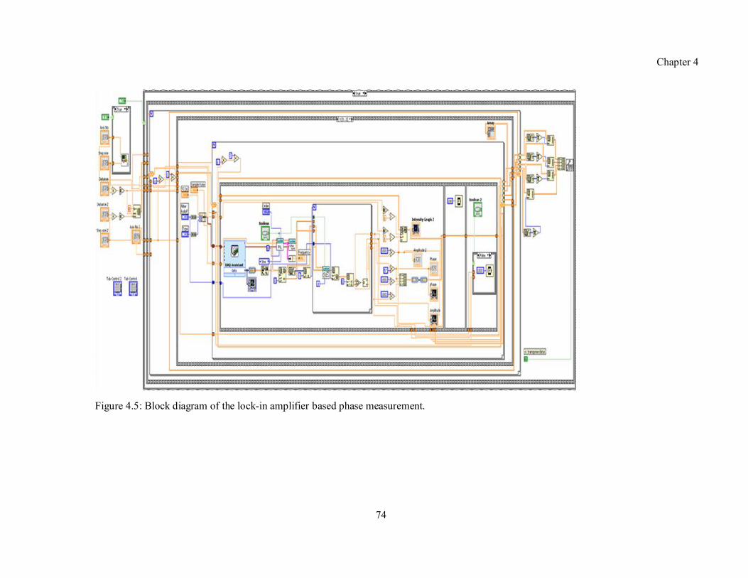
Chapter 4

74

Figure 4.5: Block diagram of the lock­in amplifier based phase measurement.

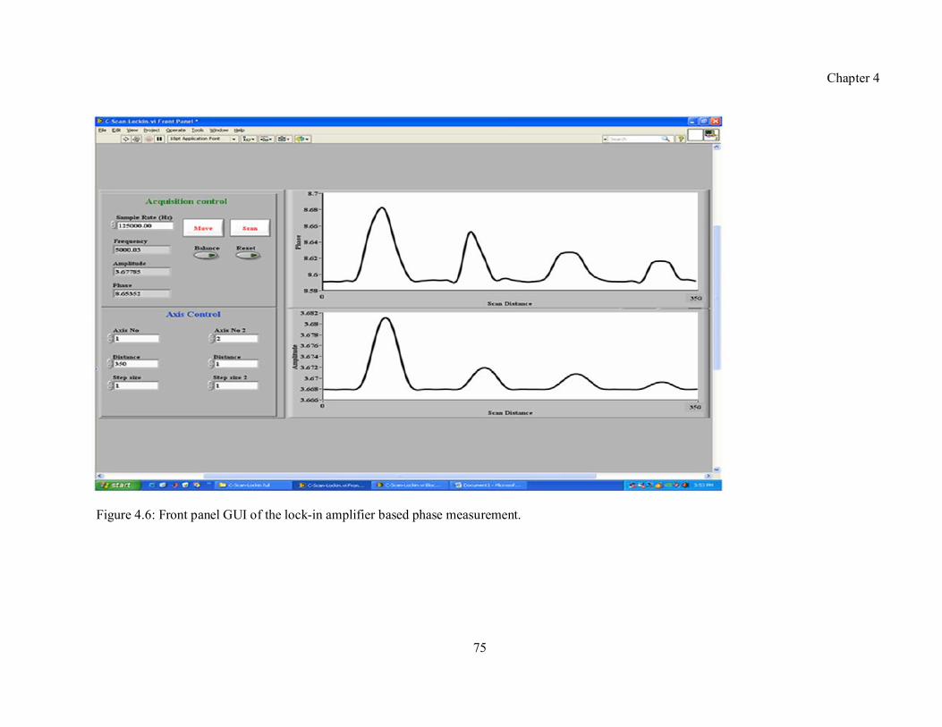
Chapter 4

75

Figure 4.6: Front panel GUI of the lock­in amplifier based phase measurement.

Chapter 4

76

4.3 Test specimens for experiments

The test specimens of size 350.0×70.0×12.0 mm3 plate made of AISI type 304L stainless steel are

used for verifying the performance of EC probe and instrument developed. For evaluation of the

instrument, flat bottom holes and notches are introduced in three 12.0 mm thick SS plates by electro

discharge machining. A schematic of three plates is shown in Figure 4.7. Four numbers of flat

bottom holes of diameter 3.0 mm at different depths in the range of 5.0 mm to 8.0 mm are used to

simulate sub­surface localized corrosion and they are fabricated in a plate as shown in Figure 4.7 (a).

A set of four notches of length 30.0 mm and width 2.5 mm at different depths in the range of 5.0 mm

to 8.0 mm and another set of three notches of length 20.0 mm and width 1.0 mm at different depths

i.e. 4.0 mm, 6.0 mm and 8.0 mm are fabricated in two plates and their details are shown in Figure

4.7 (b-c). For studies related to surface flaws, experiments are performed on opposite side of the

plate i.e. by flipping the plate. The dimensions of the flat bottom holes and machined notches

introduced in the 12.0 mm thick SS plates are given in Table 4.1 and Table 4.2.

Table 4.1: Dimensions of machined notches in SS 304L plate.

S. No Flaw Length, mm Width, mm Flaw depth (d),

mm

Depth below the

surface (D), mm

1. Notch 1 (D1) 30.0 2.5 7.0 5.0

2. Notch 2 (D2)) 30.0 2.5 6.0 6.0

3. Notch 3 (D3) 30.0 2.5 5.0 7.0

4. Notch 4 (D4) 30.0 2.5 4.0 8.0

5. Notch 5 (D5) 20.0 1.0 8.0 4.0

6. Notch 6 (D6)) 20.0 1.0 6.0 6.0

7. Notch 7 (D7) 20.0 1.0 4.0 8.0

8. Notch 4 (S1) 20.0 1.0 8.0 0.0

9. Notch 5 (S2) 20.0 1.0 6.0 0.0

10. Notch 6 (S3) 20.0 1.0 4.0 0.0

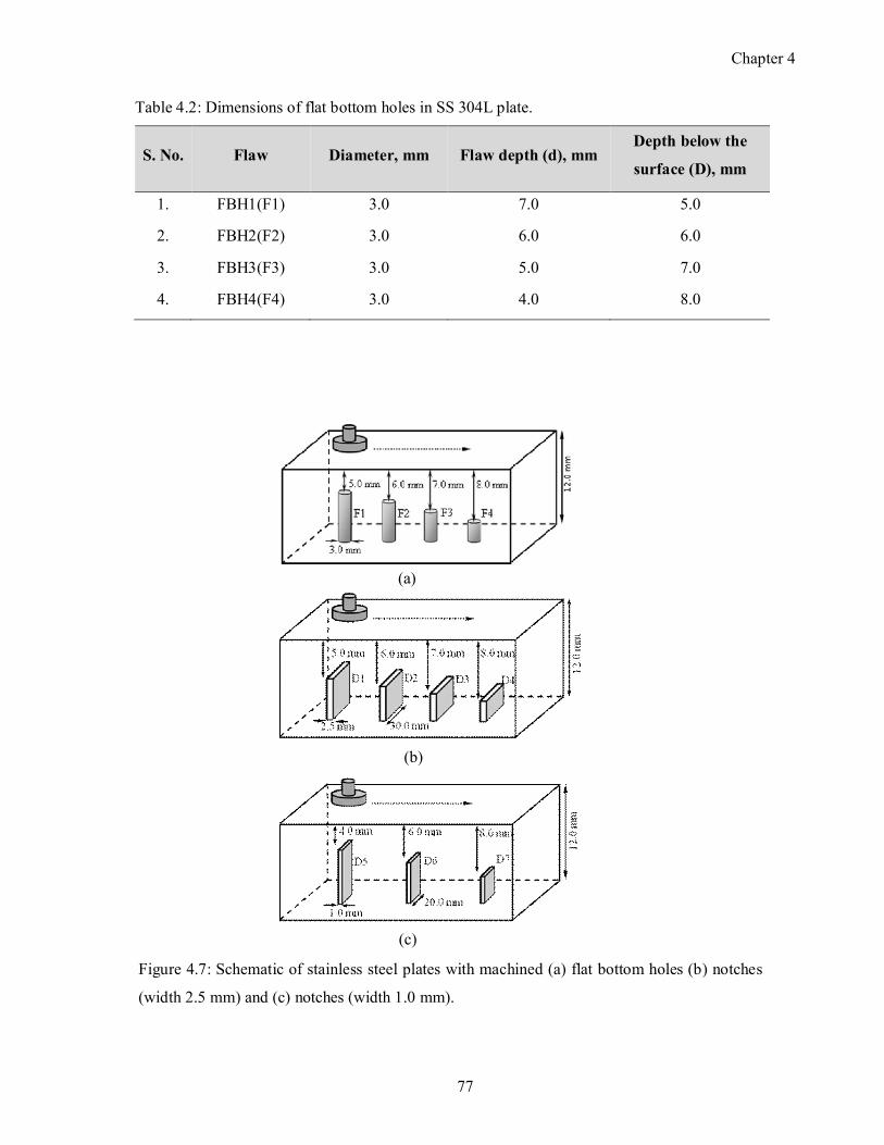
Chapter 4

77

Table 4.2: Dimensions of flat bottom holes in SS 304L plate.

S. No. Flaw Diameter, mm Flaw depth (d), mm Depth below the

surface (D), mm

1. FBH1(F1) 3.0 7.0 5.0

2. FBH2(F2) 3.0 6.0 6.0

3. FBH3(F3) 3.0 5.0 7.0

4. FBH4(F4) 3.0 4.0 8.0

(c)

Figure 4.7: Schematic of stainless steel plates with machined (a) flat bottom holes (b) notches

(width 2.5 mm) and (c) notches (width 1.0 mm).

(a)

(b)

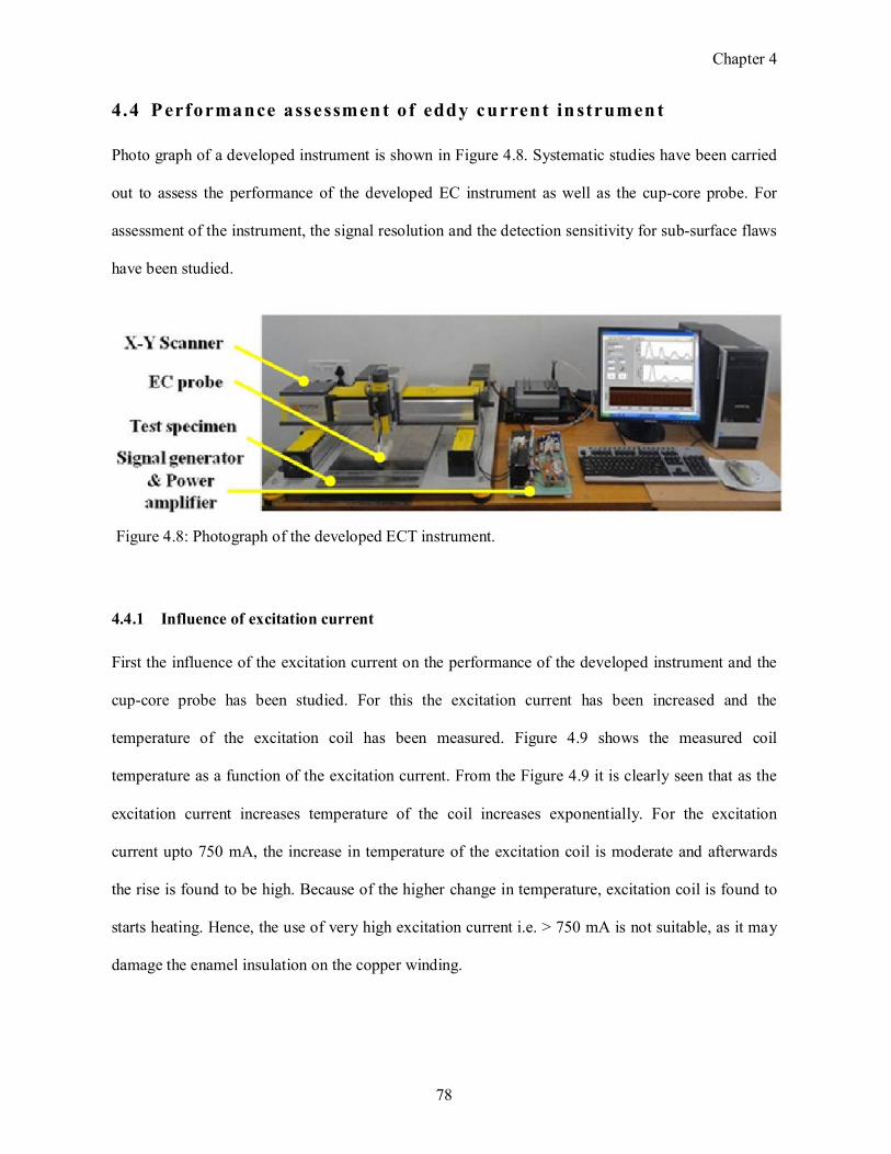
Chapter 4

78

4.4 Performance assessment of eddy current instrument

Photo graph of a developed instrument is shown in Figure 4.8. Systematic studies have been carried

out to assess the performance of the developed EC instrument as well as the cup­core probe. For

assessment of the instrument, the signal resolution and the detection sensitivity for sub­surface flaws

have been studied.

4.4.1 Influence of excitation current

First the influence of the excitation current on the performance of the developed instrument and the

cup­core probe has been studied. For this the excitation current has been increased and the

temperature of the excitation coil has been measured. Figure 4.9 shows the measured coil

temperature as a function of the excitation current. From the Figure 4.9 it is clearly seen that as the

excitation current increases temperature of the coil increases exponentially. For the excitation

current upto 750 mA, the increase in temperature of the excitation coil is moderate and afterwards

the rise is found to be high. Because of the higher change in temperature, excitation coil is found to

starts heating. Hence, the use of very high excitation current i.e. > 750 mA is not suitable, as it may

damage the enamel insulation on the copper winding.

Figure 4.8: Photograph of the developed ECT instrument.

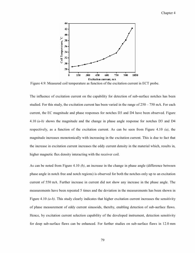
Chapter 4

79

The influence of excitation current on the capability for detection of sub­surface notches has been

studied. For this study, the excitation current has been varied in the range of 250 – 750 mA. For each

current, the EC magnitude and phase responses for notches D3 and D4 have been observed. Figure

4.10 (a-b) shows the magnitude and the change in phase angle response for notches D3 and D4

respectively, as a function of the excitation current. As can be seen from Figure 4.10 (a), the

magnitude increases monotonically with increasing in the excitation current. This is due to fact that

the increase in excitation current increases the eddy current density in the material which, results in,

higher magnetic flux density interacting with the receiver coil.

As can be noted from Figure 4.10 (b), an increase in the change in phase angle (difference between

phase angle in notch free and notch regions) is observed for both the notches only up to an excitation

current of 550 mA. Further increase in current did not show any increase in the phase angle. The

measurements have been repeated 5 times and the deviation in the measurements has been shown in

Figure 4.10 (a-b). This study clearly indicates that higher excitation current increases the sensitivity

of phase measurement of eddy current sinusoids, thereby, enabling detection of sub­surface flaws.

Hence, by excitation current selection capability of the developed instrument, detection sensitivity

for deep sub­surface flaws can be enhanced. For further studies on sub­surface flaws in 12.0 mm

Figure 4.9: Measured coil temperature as function of the excitation current in ECT probe.

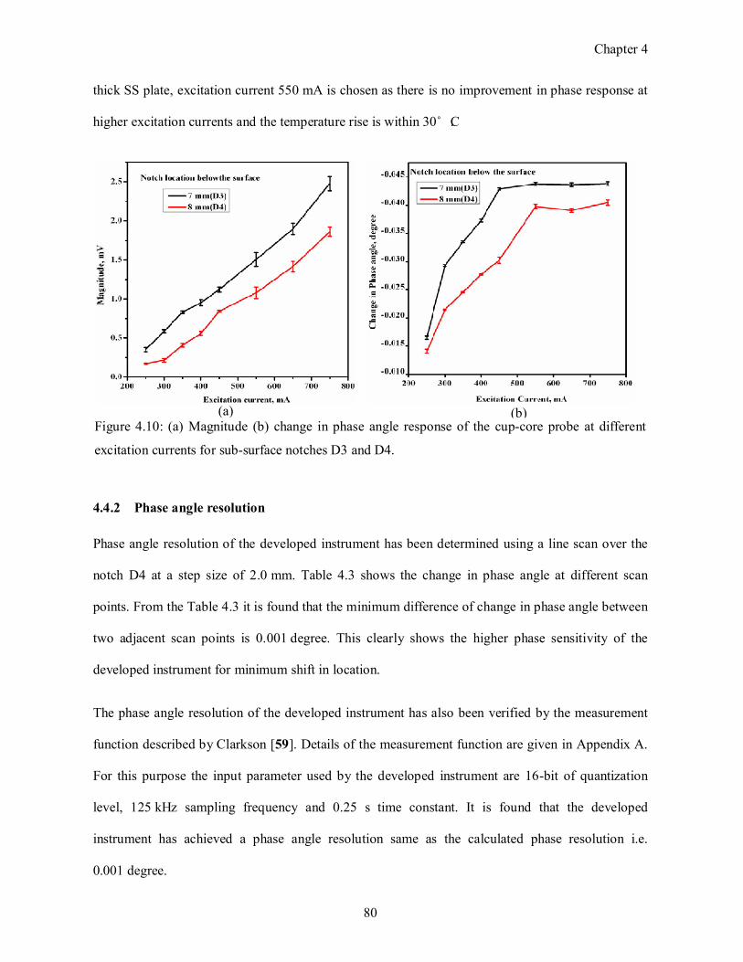
Chapter 4

80

thick SS plate, excitation current 550 mA is chosen as there is no improvement in phase response at

higher excitation currents and the temperature rise is within 30˚C.

4.4.2 Phase angle resolution

Phase angle resolution of the developed instrument has been determined using a line scan over the

notch D4 at a step size of 2.0 mm. Table 4.3 shows the change in phase angle at different scan

points. From the Table 4.3 it is found that the minimum difference of change in phase angle between

two adjacent scan points is 0.001 degree. This clearly shows the higher phase sensitivity of the

developed instrument for minimum shift in location.

The phase angle resolution of the developed instrument has also been verified by the measurement

function described by Clarkson [59]. Details of the measurement function are given in Appendix A.

For this purpose the input parameter used by the developed instrument are 16­bit of quantization

level, 125 kHz sampling frequency and 0.25 s time constant. It is found that the developed

instrument has achieved a phase angle resolution same as the calculated phase resolution i.e.

0.001 degree.

(a) (b) Figure 4.10: (a) Magnitude (b) change in phase angle response of the cup­core probe at different

excitation currents for sub­surface notches D3 and D4.

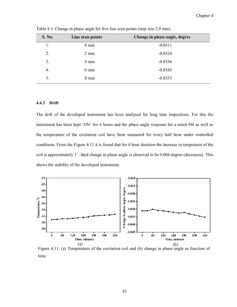
Chapter 4

81

Table 4.3: Change in phase angle for five line scan points (step size 2.0 mm).

S. No. Line scan points Change in phase angle, degree

1. 0 mm ­0.0311

2. 2 mm ­0.0324

3. 4 mm ­0.0336

4. 6 mm ­0.0345

5. 8 mm ­0.0353

4.4.3 Drift

The drift of the developed instrument has been analysed for long time inspections. For this the

instrument has been kept ‘ON’ for 6 hours and the phase angle response for a notch D4 as well as

the temperature of the excitation coil have been measured for every half hour under controlled

conditions. From the Figure 4.11 it is found that for 6 hour duration the increase in temprature of the

coil is approximately 1˚C and change in phase angle is observed to be 0.004 degree (decreases). This

shows the stability of the developed instrument.

Figure 4.11: (a) Temperature of the excitation coil and (b) change in phase angle as function of

time.

(a) (b)

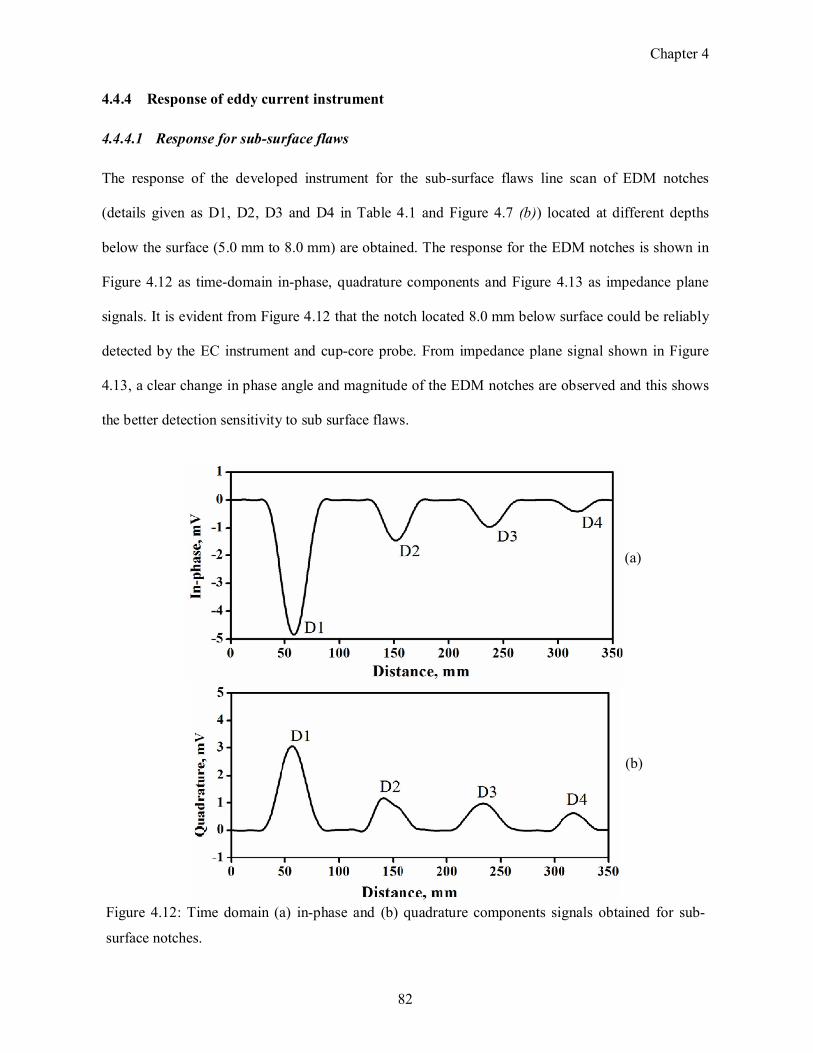
Chapter 4

82

4.4.4 Response of eddy current instrument

4.4.4.1 Response for sub-surface flaws

The response of the developed instrument for the sub­surface flaws line scan of EDM notches

(details given as D1, D2, D3 and D4 in Table 4.1 and Figure 4.7 (b)) located at different depths

below the surface (5.0 mm to 8.0 mm) are obtained. The response for the EDM notches is shown in

Figure 4.12 as time­domain in­phase, quadrature components and Figure 4.13 as impedance plane

signals. It is evident from Figure 4.12 that the notch located 8.0 mm below surface could be reliably

detected by the EC instrument and cup­core probe. From impedance plane signal shown in Figure

4.13, a clear change in phase angle and magnitude of the EDM notches are observed and this shows

the better detection sensitivity to sub surface flaws.

Figure 4.12: Time domain (a) in­phase and (b) quadrature components signals obtained for sub­

surface notches.

(a)

(b)

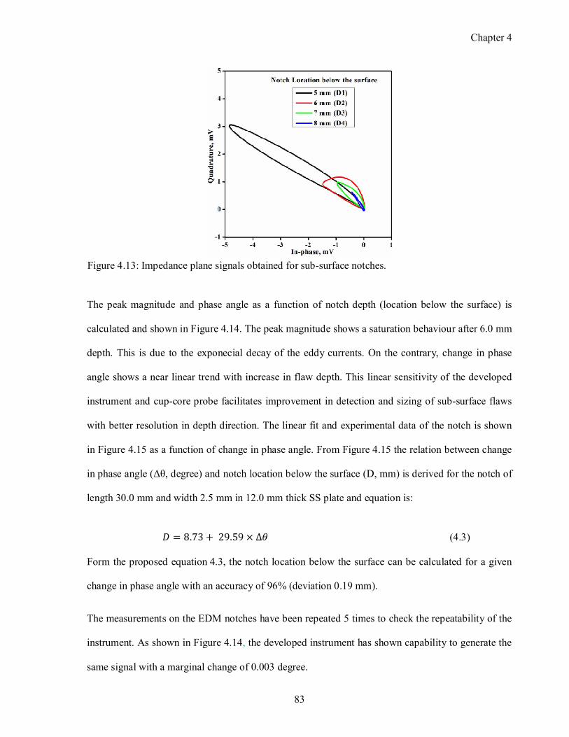
Chapter 4

83

The peak magnitude and phase angle as a function of notch depth (location below the surface) is

calculated and shown in Figure 4.14. The peak magnitude shows a saturation behaviour after 6.0 mm

depth. This is due to the exponecial decay of the eddy currents. On the contrary, change in phase

angle shows a near linear trend with increase in flaw depth. This linear sensitivity of the developed

instrument and cup­core probe facilitates improvement in detection and sizing of sub­surface flaws

with better resolution in depth direction. The linear fit and experimental data of the notch is shown

in Figure 4.15 as a function of change in phase angle. From Figure 4.15 the relation between change

in phase angle (Δθ, degree) and notch location below the surface (D, mm) is derived for the notch of

length 30.0 mm and width 2.5 mm in 12.0 mm thick SS plate and equation is:

� = 8.73 + 29.59 × ∆� (4.3)

Form the proposed equation 4.3, the notch location below the surface can be calculated for a given

change in phase angle with an accuracy of 96% (deviation 0.19 mm).

The measurements on the EDM notches have been repeated 5 times to check the repeatability of the

instrument. As shown in Figure 4.14, the developed instrument has shown capability to generate the

same signal with a marginal change of 0.003 degree.

Figure 4.13: Impedance plane signals obtained for sub­surface notches.

Chapter 4

84

4.4.4.2 Comparison with commercial instrument

Response of the developed instrument has been compared with a commercial general purpose ECT

instrument (TECHNOFOUR INSIS EX­4). This is a constant current instrument (300 mA). As the

commercial instrument is not capable of measuring the absolute phase lag of the receiver coil

Figure 4.15: Linear behavior of notch location below the surface (D) as function of change in phase

angle (Δθ).

(a) (b)

Figure 4.14: (a) Peak magnitude and (b) peak of change in phase angle of sub­surface notches.

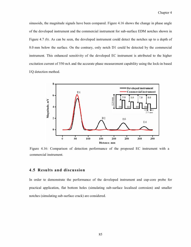
Chapter 4

85

sinusoids, the magnitude signals have been compared. Figure 4.16 shows the change in phase angle

of the developed instrument and the commercial instrument for sub­surface EDM notches shown in

Figure 4.7 (b). As can be seen, the developed instrument could detect the notches up to a depth of

8.0 mm below the surface. On the contrary, only notch D1 could be detected by the commercial

instrument. This enhanced sensitivity of the developed EC instrument is attributed to the higher

excitation current of 550 mA and the accurate phase measurement capability using the lock­in based

I/Q detection method.

4.5 Results and discussion

In order to demonstrate the performance of the developed instrument and cup­core probe for

practical application, flat bottom holes (simulating sub­surface localised corrosion) and smaller

notches (simulating sub­surface crack) are considered.

Figure 4.16: Comparison of detection performance of the proposed EC instrument with a

commercial instrument.

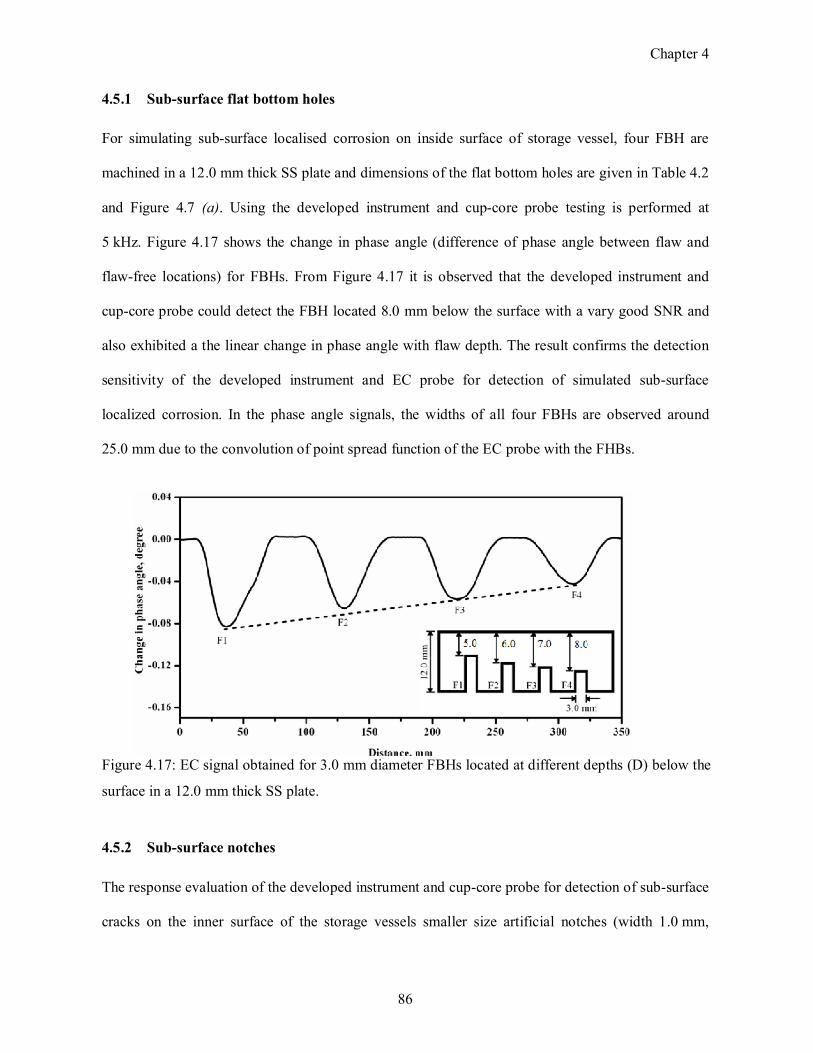
Chapter 4

86

4.5.1 Sub-surface flat bottom holes

For simulating sub­surface localised corrosion on inside surface of storage vessel, four FBH are

machined in a 12.0 mm thick SS plate and dimensions of the flat bottom holes are given in Table 4.2

and Figure 4.7 (a). Using the developed instrument and cup­core probe testing is performed at

5 kHz. Figure 4.17 shows the change in phase angle (difference of phase angle between flaw and

flaw­free locations) for FBHs. From Figure 4.17 it is observed that the developed instrument and

cup­core probe could detect the FBH located 8.0 mm below the surface with a vary good SNR and

also exhibited a the linear change in phase angle with flaw depth. The result confirms the detection

sensitivity of the developed instrument and EC probe for detection of simulated sub­surface

localized corrosion. In the phase angle signals, the widths of all four FBHs are observed around

25.0 mm due to the convolution of point spread function of the EC probe with the FHBs.

4.5.2 Sub-surface notches

The response evaluation of the developed instrument and cup­core probe for detection of sub­surface

cracks on the inner surface of the storage vessels smaller size artificial notches (width 1.0 mm,

Figure 4.17: EC signal obtained for 3.0 mm diameter FBHs located at different depths (D) below the

surface in a 12.0 mm thick SS plate.

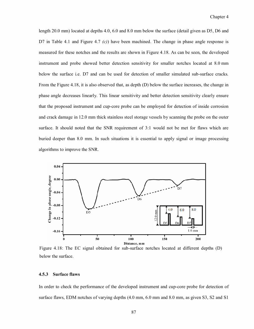
Chapter 4

87

length 20.0 mm) located at depths 4.0, 6.0 and 8.0 mm below the surface (detail given as D5, D6 and

D7 in Table 4.1 and Figure 4.7 (c)) have been machined. The change in phase angle response is

measured for these notches and the results are shown in Figure 4.18. As can be seen, the developed

instrument and probe showed better detection sensitivity for smaller notches located at 8.0 mm

below the surface i.e. D7 and can be used for detection of smaller simulated sub­surface cracks.

From the Figure 4.18, it is also observed that, as depth (D) below the surface increases, the change in

phase angle decreases linearly. This linear sensitivity and better detection sensitivity clearly ensure

that the proposed instrument and cup­core probe can be employed for detection of inside corrosion

and crack damage in 12.0 mm thick stainless steel storage vessels by scanning the probe on the outer

surface. It should noted that the SNR requirement of 3:1 would not be met for flaws which are

buried deeper than 8.0 mm. In such situations it is essential to apply signal or image processing

algorithms to improve the SNR.

4.5.3 Surface flaws

In order to check the performance of the developed instrument and cup­core probe for detection of

surface flaws, EDM notches of varying depths (4.0 mm, 6.0 mm and 8.0 mm, as given S3, S2 and S1

Figure 4.18: The EC signal obtained for sub­surface notches located at different depths (D)

below the surface.

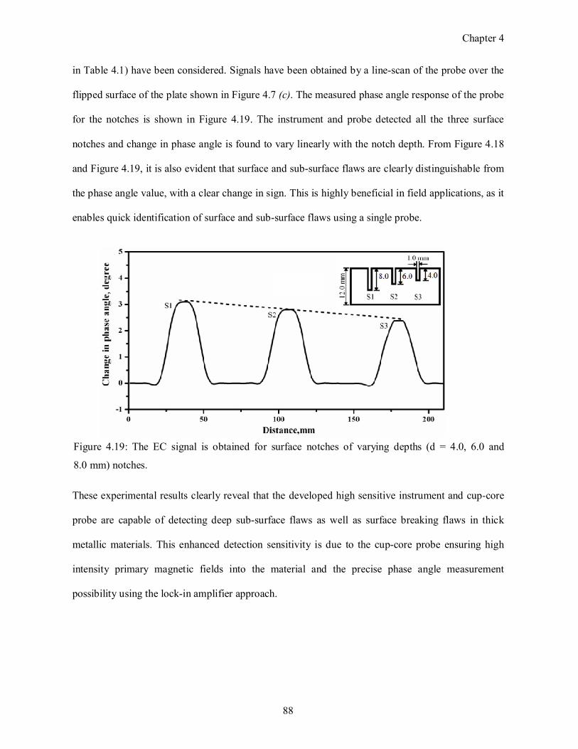
Chapter 4

88

in Table 4.1) have been considered. Signals have been obtained by a line­scan of the probe over the

flipped surface of the plate shown in Figure 4.7 (c). The measured phase angle response of the probe

for the notches is shown in Figure 4.19. The instrument and probe detected all the three surface

notches and change in phase angle is found to vary linearly with the notch depth. From Figure 4.18

and Figure 4.19, it is also evident that surface and sub­surface flaws are clearly distinguishable from

the phase angle value, with a clear change in sign. This is highly beneficial in field applications, as it

enables quick identification of surface and sub­surface flaws using a single probe.

These experimental results clearly reveal that the developed high sensitive instrument and cup­core

probe are capable of detecting deep sub­surface flaws as well as surface breaking flaws in thick

metallic materials. This enhanced detection sensitivity is due to the cup­core probe ensuring high

intensity primary magnetic fields into the material and the precise phase angle measurement

possibility using the lock­in amplifier approach.

Figure 4.19: The EC signal is obtained for surface notches of varying depths (d = 4.0, 6.0 and

8.0 mm) notches.

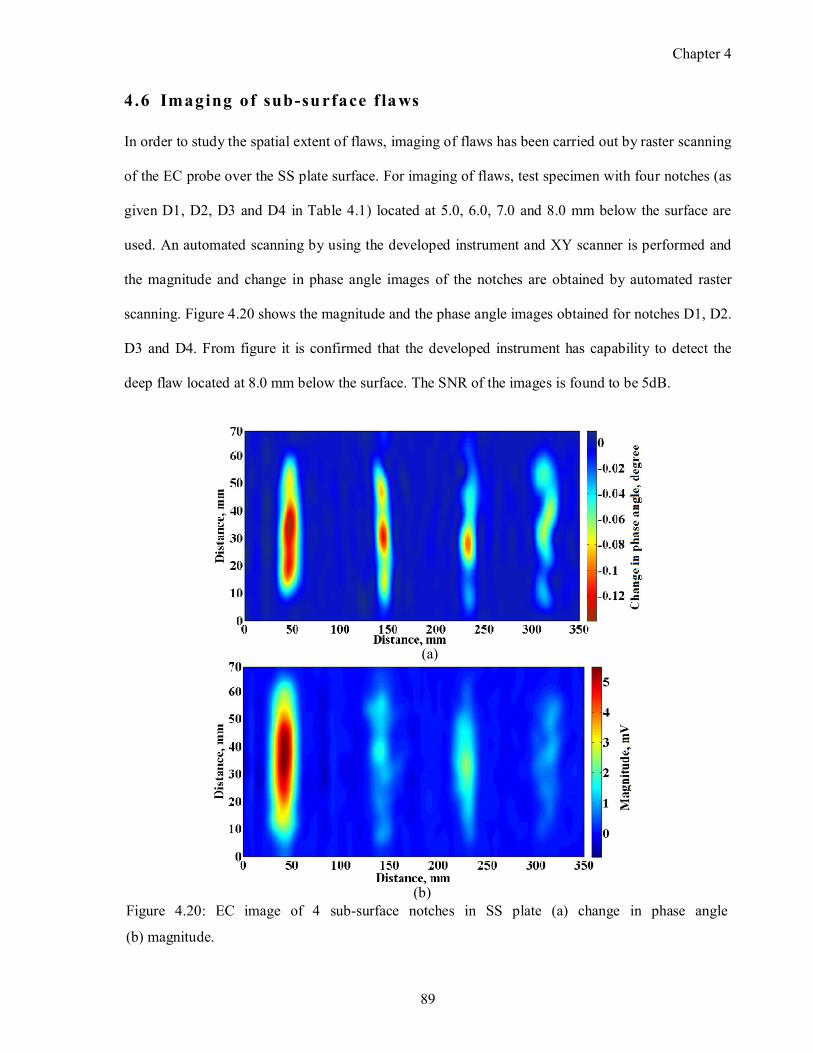
Chapter 4

89

4.6 Imaging of sub-surface f laws

In order to study the spatial extent of flaws, imaging of flaws has been carried out by raster scanning

of the EC probe over the SS plate surface. For imaging of flaws, test specimen with four notches (as

given D1, D2, D3 and D4 in Table 4.1) located at 5.0, 6.0, 7.0 and 8.0 mm below the surface are

used. An automated scanning by using the developed instrument and XY scanner is performed and

the magnitude and change in phase angle images of the notches are obtained by automated raster

scanning. Figure 4.20 shows the magnitude and the phase angle images obtained for notches D1, D2.

D3 and D4. From figure it is confirmed that the developed instrument has capability to detect the

deep flaw located at 8.0 mm below the surface. The SNR of the images is found to be 5dB.

(a)

(b) Figure 4.20: EC image of 4 sub­surface notches in SS plate (a) change in phase angle

(b) magnitude.

Chapter 4

90

From the EC images shown in Figure 4.20 presence of flaws can be observed. However, for reliable

detection and sizing of flaws, this is a need to enhance the SNR and resolution in the EC images. For

this purpose fusion of the images has been attempted and the details are discussed in Chapter 5.0.

4.7 Summary

A high sensitive eddy current instrument has been developed for detection of sub­surface flaws in

12.0 mm thick stainless steel plate. Systematic studies using the instrument reveal a definite

improvement in the detection sensitivity, as a result of increase in the excitation current and by the

use of precise phase angle measurement. The observed results are the following:

For AISI 304L stainless steel plate of thickness 12.0 mm, an excitation current of 550 mA has

ensured unambiguous detection of sub­surface notch located at 8.0 mm below the surface.

The higher current driving capacity complied with the high dynamic range of the lock­in based

I/Q detection method enabled detection of the sub­surface notches in 12.0 mm thick AISI 304L

stainless steel plate.

The developed instrument and probe resulted in a linear relationship between the depth below

the surface and change in phase angle. This linear sensitivity facilitates accurate detection and

sizing of deep sub­surface flaws with better resolution in the depth direction (thickness).

This study established, for the first time, that it is possible to distinguish surface and sub­surface

flaws from the change in the phase angle signals, as they are well separated in sign.

The high sensitive eddy current instrument and cup­core type send­receive probe promise better

sensitivity for detection of simulated sub­surface localized corrosion as well as simulated sub­

surface crack.

91

Development of image fusion

methodology

5 .1 Preamble

This chapter presents a novel image fusion methodology for enhancing the detection capability of

the proposed instrument and optimized probe. The methodology is based on the combined

advantages of wavelet transform (time­frequency) and Bayesian (statistical) methodologies. The

performance of the proposed fusion methodology has been compared with other existing fusion

methodologies such as Laplacian pyramid, wavelet transform, PCA and Bayesian, based on image

metrics such as standard deviation, SNR, entropy and fusion mutual information.

5.2 Image fusion

As explained in Section 1.3.7 wavelet transform fusion methodology is based on multi­resolution

analysis, where the source images are decomposed into a set of sub­sampled images in spatial

frequency. These sub­sampled images represent unique information at different frequency as well as

resolution level and provide the information about edges of flaws in EC images (source image).

These edges of flaw define the extent of flaw, which is essential for detection and characterization.

Hence, application of wavelet transform based methodology is beneficial when the image contains

reasonably well delineated frequency components between the desired features (flaw) and noise.

Studies reveal that wavelet transform based fusion methodology when applied to EC images resulted

in better localization of the flaws. However the improvement in SNR is not significant [33]. This is

due to the fact that the noise does not have well defined frequency components. Statistical

methodologies are attractive in this context.

5

Chapter 5

92

The statistical inference based Bayesian fusion methodology provides a probability of hypothesis

being true for given evidence or prior probability. The prior probability which is the prior

information of the likelihood of the flaw and noise information in the images and is derived mostly

based on expert knowledge. Determination of the prior probability is a key issue in the Bayesian

methodology.

It should be noted that the EC images of sub­surface flaws are influenced by disturbing noise from

various sources such as lift­off, material property and instrumentation. It is understood that the noise

due to lift­off variations has well defined frequency components that are different from the flaw. On

the other hand, the noise due to material property variations and instrument are random in nature. In

addition to the noise having well defined frequency components, there exist randomness of the noise

in EC images. Hence, the fusion methodology adopted should derive the mutual benefits of the time­

frequency methods and statistical based methods towards enhancing the SNR of the EC images of

sub­surface flaws. In this context, a new Bayesian and wavelet transformed (BayWT) based image

fusion methodology that utilizes the advantages of the wavelet transform methodology as well as

Bayesian based fusion methodology.

5.3 Proposed BayWT based image fus ion methodology

The schematic block diagram of the proposed BayWT image fusion methodology is shown in Figure

5.1. In this methodology the source images are first decomposed into sub­sampled images by

discrete wavelet transform (by using equation 1.14) as the sub­sampled images. These sub­sampled

images provide the spectral information about the flaw location. This information is used for

formulation the prior probability for the Bayesian based image fusion. For this purpose, a zero mean

and unit standard deviation Gaussian function has been correlated with each sub­sampled wavelet

images and correlated Gaussian function matrix is formulated as prior knowledge. This process

would maximize the probabilities of detection of flaws, as a typical shape of flaw image is Gaussian

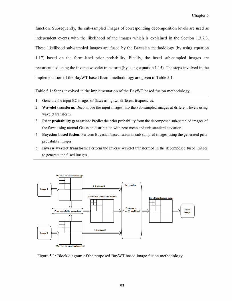
Chapter 5

93

function. Subsequently, the sub­sampled images of corresponding decomposition levels are used as

independent events with the likelihood of the images which is explained in the Section 1.3.7.3.

These likelihood sub­sampled images are fused by the Bayesian methodology (by using equation

1.17) based on the formulated prior probability. Finally, the fused sub­sampled images are

reconstructed using the inverse wavelet transform (by using equation 1.15). The steps involved in the

implementation of the BayWT based fusion methodology are given in Table 5.1.

Table 5.1: Steps involved in the implementation of the BayWT based fusion methodology.

1. Generate the input EC images of flaws using two different frequencies.

2. Wavelet transform: Decompose the input images into the sub­sampled images at different levels using

wavelet transform.

3. Prior probability generation: Predict the prior probability from the decomposed sub­sampled images of

the flaws using normal Gaussian distribution with zero mean and unit standard deviation.

4. Bayesian based fusion: Perform Bayesian based fusion in sub­sampled images using the generated prior

probability images.

5. Inverse wavelet transform: Perform the inverse wavelet transformed in the decomposed fused images

to generate the fused images.

Figure 5.1: Block diagram of the proposed BayWT based image fusion methodology.

Chapter 5

94

5.4 Input eddy current images

Image fusion studies have been carried out by using numerical model generated EC images of sub­

surface flaws. The proposed image fusion methodology has been validated for one case, using

experimentally generated EC images of a flaw.

CIVA software which is benchmarked numerical modeling software for NDE techniques has been

used for generation of EC images of sub­surface flaws [93]. Using CIVA software, EC images of

sub­surface notch of length 30.0 mm and width 2.5 mm with depths ranging from 5.0 mm to 8.0 mm

below the surface of a 12.0 mm thick stainless steel plate have been predicted at 5 kHz and 7 kHz

frequency for the optimized cup­core probe. Further, phase angle images of a sub­surface notch (D4)

located 8.0 mm below the surface (as given in Figure 4.7 (b)) at frequency 5 kHz and 7 kHz have

been generated using the developed ECT instrument and cup­core probe. These generated images

have been used for evaluation of the proposed image fusion methodology. In order to simulate

experimental noise, white Gaussian noise (noise level is 30% of the maximum amplitude) has been

added to the model predicted images according to a predefined SNR.

5.5 Performance evaluation of BayWT image fus ion

Performance evaluation of fusion methodologies are usually carried out based on two classes. First is

the subjective evaluation metric, which depends on the human vision system (HVS). In this class, a

qualitative assessment of the fused image based on the visibility of the features is made by human.

Second class is the objective evaluation metrics. Objective metrics are quantitatively measure of the

human perception. There are several metrics presents for assessments of the images objectively and

they classified in to two categories, first one required a reference image while other do not [70,29].

For objective evaluation of the fused image, the following metrics have been used.

1) Standard deviation

Chapter 5

95

2) Entropy

3) Signal­to­noise ratio (SNR)

4) Fusion mutual information (FMI).

Standard deviation, entropy and SNR metrics do not use reference image. But the Fusion mutual

information metric use source images as reference.

5.5.1 Standard deviation

Standard deviation is a statistical quantity, which is used to measure the amount of variability or

dispersion around the mean of the image. It is a measure of the image contrast and is defined as the

square root of the variance as given in equation 5.1 below:

�������� ��������� (�)= �� �(�(�,�)− �)�

��

�

���

�

���

(5.1)

where � = 1

��� � �(�,�)

�

���

�

���

(5.2)

where I is the image, � is the mean of the image, M and N refers to the maximum number of pixels

in the image in horizontal and vertical direction respectively and i and j are the indices which refers

to the individual pixels of the image. Image contrast depends on the range of the data. An image

with high contrast would have a high standard deviation, because of the higher dispersion (higher

range of data) around the mean of the image.

5.5.2 Entropy

The entropy of an image describes the amount of information present in the image. The entropy (H)

of the image is defined as

Chapter 5

96

� = − � � �(�,�)

�

���

log� �(�,�)

�

���

(5.3)

where P is the probability of intensity at pixel level of image. Entropy is sensitive to noise and other

unwanted rapid fluctuations in the image. Low entropy images have very little contrast and large

number of redundant data. But the higher value of entropy shows the contrast in images and higher

information content.

5.5.3 Signal-to-noise ratio

Definition of SNR generally depends on the application. In the present study, the SNR is defined as

the ratio of mean or expected value of flaw signal (�������) to the standard deviation of the noise

(������) in the image and define as:

��� = 10 log��

�������

������ (5.4)

The SNR will tend to infinity when the flaw image is free from noise. Image with high SNR

provides the better quality image. Hence, the image with high SNR value is preferred.

5.5.4 Fusion mutual information

Mutual information (MI) is a metric which is used to measure the degree of dependency of the two

images A and B by measuring the distance between the joint distribution PA,B and the distribution

associated with the case of complete independence PA PB. The amount of information corresponding

to these features, calculated from the source images to the fused image, can be a suitable to evaluate

the performance of the fusion methodology. The MI of two images A and B can define as:

�� (�,�) = � � ��,�(�,�)

�

���

�

���

log� ���,�(�,�)

��(�,�)� �(�,�)� (5.5)

By this, dependency between the fused image and the source image can be measured independently.

In this study, the mutual information of the fused image with source images A and B has been

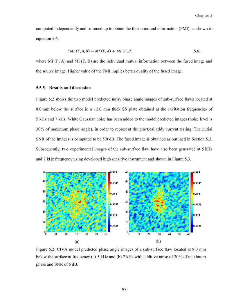
Chapter 5

97

computed independently and summed up to obtain the fusion mutual information (FMI) as shown in

equation 5.6:

��� (�,�,�) = �� (�,�)+ �� (�,�) (5.6)

where MI (F, A) and MI (F, B) are the individual mutual information between the fused image and

the source image. Higher value of the FMI implies better quality of the fused image.

5.5.5 Results and discussion

Figure 5.2 shows the two model predicted noisy phase angle images of sub­surface flaws located at

8.0 mm below the surface in a 12.0 mm thick SS plate obtained at the excitation frequencies of

5 kHz and 7 kHz. White Gaussian noise has been added to the model predicted images (noise level is

30% of maximum phase angle), in order to represent the practical eddy current testing. The initial

SNR of the images is computed to be 5.0 dB. The fused image is obtained as outlined in Section 5.3.

Subsequently, two experimental images of the sub­surface flaw have also been generated at 5 kHz

and 7 kHz frequency using developed high sensitive instrument and shown in Figure 5.3.

(a) (b)

Figure 5.2: CIVA model predicted phase angle images of a sub­surface flaw located at 8.0 mm

below the surface at frequency (a) 5 kHz and (b) 7 kHz with additive noise of 30% of maximum

phase and SNR of 5 dB.

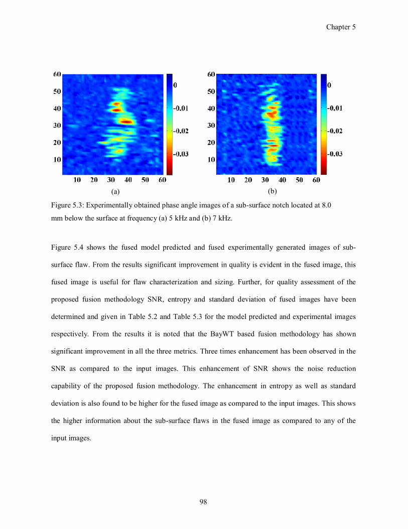
Chapter 5

98

Figure 5.4 shows the fused model predicted and fused experimentally generated images of sub­

surface flaw. From the results significant improvement in quality is evident in the fused image, this

fused image is useful for flaw characterization and sizing. Further, for quality assessment of the

proposed fusion methodology SNR, entropy and standard deviation of fused images have been

determined and given in Table 5.2 and Table 5.3 for the model predicted and experimental images

respectively. From the results it is noted that the BayWT based fusion methodology has shown

significant improvement in all the three metrics. Three times enhancement has been observed in the

SNR as compared to the input images. This enhancement of SNR shows the noise reduction

capability of the proposed fusion methodology. The enhancement in entropy as well as standard

deviation is also found to be higher for the fused image as compared to the input images. This shows

the higher information about the sub­surface flaws in the fused image as compared to any of the

input images.

(a) (b)

Figure 5.3: Experimentally obtained phase angle images of a sub­surface notch located at 8.0

mm below the surface at frequency (a) 5 kHz and (b) 7 kHz.

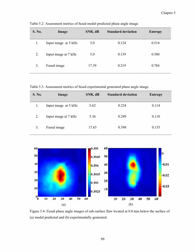
Chapter 5

99

Table 5.2: Assessment metrics of fused model predicted phase angle image.

S. No. Image SNR, dB Standard deviation Entropy

1. Input image at 5 kHz 5.0 0.124 0.514

2. Input image at 7 kHz 5.0 0.139 0.580

3. Fused image 17.39 0.219 0.784

Table 5.3: Assessment metrics of fused experimental generated phase angle image.

S. No. Image SNR, dB Standard deviation Entropy

1. Input image at 5 kHz 5.62 0.224 0.114

2. Input image at 7 kHz 5.36 0.289 0.110

3. Fused image 17.63 0.398 0.135

(a) (b)

Figure 5.4: Fused phase angle images of sub­surface flaw located at 8.0 mm below the surface of

(a) model predicted and (b) experimentally generated.

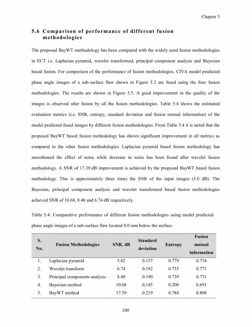
Chapter 5

100

5.6 Comparison of performance of dif ferent fusion methodologies

The proposed BayWT methodology has been compared with the widely used fusion methodologies

in ECT i.e. Laplacian pyramid, wavelet transformed, principal component analysis and Bayesian

based fusion. For comparison of the performance of fusion methodologies, CIVA model predicted

phase angle images of a sub­surface flaw shown in Figure 5.2 are fused using the four fusion

methodologies. The results are shown in Figure 5.5. A good improvement in the quality of the

images is observed after fusion by all the fusion methodologies. Table 5.4 shows the estimated

evaluation metrics (i.e. SNR, entropy, standard deviation and fusion mutual information) of the

model predicted fused images by different fusion methodologies. From Table 5.4 it is noted that the

proposed BayWT based fusion methodology has shown significant improvement in all metrics as

compared to the other fusion methodologies. Laplacian pyramid based fusion methodology has

smoothened the effect of noise while decrease in noise has been found after wavelet fusion

methodology. A SNR of 17.39 dB improvement is achieved by the proposed BayWT based fusion

methodology. This is approximately three times the SNR of the input images (5.0 dB). The

Bayesian, principal component analysis and wavelet transformed based fusion methodologies

achieved SNR of 10.68, 8.48 and 6.74 dB respectively.

Table 5.4: Comparative performance of different fusion methodologies using model predicted

phase angle images of a sub­surface flaw located 8.0 mm below the surface.

S.

No. Fusion Methodologies SNR, dB

Standard

deviation Entropy

Fusion

mutual

information

1. Laplacian pyramid 5.82 0.157 0.779 0.734

2. Wavelet transform 6.74 0.192 0.755 0.771

3. Principal components analysis 8.48 0.190 0.739 0.731

4. Bayesian method 10.68 0.145 0.200 0.691

5. BayWT method 17.39 0.219 0.784 0.808

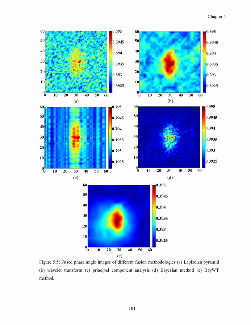
Chapter 5

101

(a) (b)

(c) (d)

(e)

Figure 5.5: Fused phase angle images of different fusion methodologies (a) Laplacian pyramid

(b) wavelet transform (c) principal component analysis (d) Bayesian method (e) BayWT

method.

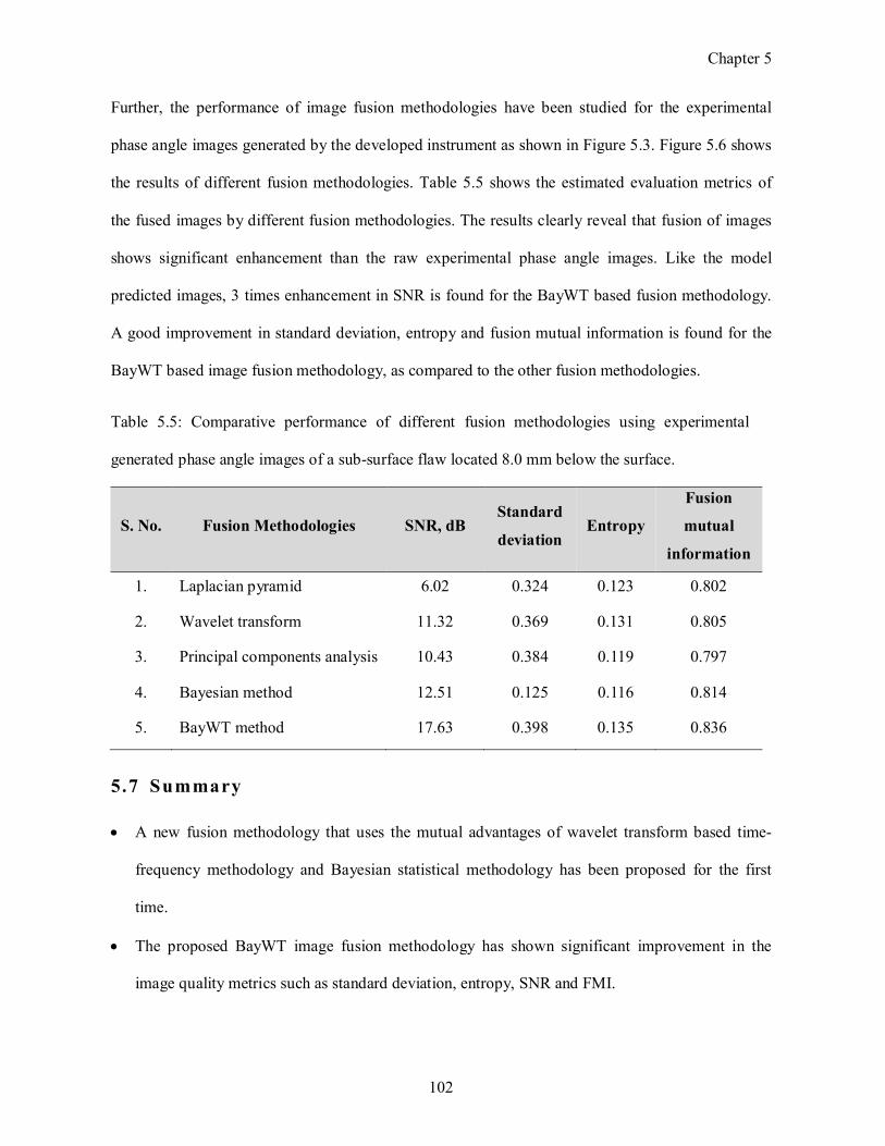
Chapter 5

102

Further, the performance of image fusion methodologies have been studied for the experimental

phase angle images generated by the developed instrument as shown in Figure 5.3. Figure 5.6 shows

the results of different fusion methodologies. Table 5.5 shows the estimated evaluation metrics of

the fused images by different fusion methodologies. The results clearly reveal that fusion of images

shows significant enhancement than the raw experimental phase angle images. Like the model

predicted images, 3 times enhancement in SNR is found for the BayWT based fusion methodology.

A good improvement in standard deviation, entropy and fusion mutual information is found for the

BayWT based image fusion methodology, as compared to the other fusion methodologies.

Table 5.5: Comparative performance of different fusion methodologies using experimental

generated phase angle images of a sub­surface flaw located 8.0 mm below the surface.

S. No. Fusion Methodologies SNR, dB Standard

deviation Entropy

Fusion

mutual

information

1. Laplacian pyramid 6.02 0.324 0.123 0.802

2. Wavelet transform 11.32 0.369 0.131 0.805

3. Principal components analysis 10.43 0.384 0.119 0.797

4. Bayesian method 12.51 0.125 0.116 0.814

5. BayWT method 17.63 0.398 0.135 0.836

5.7 Summary

A new fusion methodology that uses the mutual advantages of wavelet transform based time­

frequency methodology and Bayesian statistical methodology has been proposed for the first

time.

The proposed BayWT image fusion methodology has shown significant improvement in the

image quality metrics such as standard deviation, entropy, SNR and FMI.

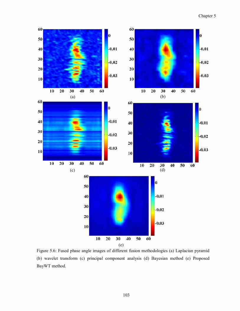
Chapter 5

103

(a) (b)

(c) (d)

(e)

Figure 5.6: Fused phase angle images of different fusion methodologies (a) Laplacian pyramid

(b) wavelet transform (c) principal component analysis (d) Bayesian method (e) Proposed

BayWT method.

Chapter 5

104

In this methodology a new way to compute the prior probability has been proposed.

The proposed BayWT based fusion methodology achieved a SNR of 17.63 dB, which is three

times the SNR of the input images (5.0 dB).

The image enhancement achieved through the proposed BayWT methodology has been found to

be higher than that of the individual fusion methodologies viz. Laplace, wavelet, Bayesian and

PCA.

105

Novel scan methodology for rapid

detection and imaging of f laws

6.1 Preamble

This chapter elucidates the results of the studies made by comparing different scan plans viz. raster,

diagonal raster, spiral, Lissajous, and billiard scan plans, towards identifying efficient and rapid scan

plan for detecting and imaging of flaws in austenitic stainless steel plates. Numerical model based

and experimental based studies carried out in this regard are also presented in this chapter.

It has been discussed in Section 1.2 and Section 1.4.4 imaging of larger area of the material is time

taking process which is a harmful for inspection personnel in radioactive environment. Hence, rapid

detection and imaging of flaw is preferred. As seen from the literature, in ECT raster scanning using

single ECT probe and line scanning using array type ECT probe are used for detection and imaging.

Although there are a few advantages of using raster scan plan or array ECT probe for detection and

imaging, a few drawbacks limit its wide spread use. Rapid detection and imaging of flaws is also

possible by scanning with single ECT probe but using different scan plans. This is employed in this

chapter.

6.2 Parameters for rapid scan plans

Any scan plan using a single ECT probe is expected to meet the following criteria for fast and

effective detection of flaws:

1. Complete coverage: the scan plan should cover the entire surface area.

2. Rapidness: the scan plan should cover the entire surface area in minimal possible time.

6

Chapter 6

106

3. Probability of detection: the scan plan should detect all the flaws present in the scan area with

good repeatability.

4. Variable step size (Δ): By increasing the step size, time for scanning decreases but probability

of detection (POD) also decreases. Hence, a scan plan should use optimal step size without

compromising the POD.

In this study, four different scan plans viz., 1) diagonal raster, 2) spiral, 3) Lissajous, and 4) billiard

have been studied , for the first time, and their performances for a rectangular scan area have been

analysed and compared with the conventional raster scan plan.

6.3 Descrip tion of the scan plans

6.3.1 Raster scan

Raster scan plan is commonly used in ECT to image flaws in plates. The raster scan can be either

horizontal or vertical. In raster scan, the scan area contains N number of line segments (referred as

scan lines) which are equally spaced with a constant step size (Δ) as shown in Figure 6.1. Raster scan

is defined by the number of line segments and the number of steps in a line segment. For example,

for a rectangular­shaped area of length (l) and width (w) with equal step size of Δ (i.e. ∆= ∆�= ∆�)

in both orthogonal directions can be described as

������ �� ���� ����� (�)= �

∆ (6.1)

������ �� ����� �� ��� ���� ���� (�)= �

∆ (6.2)

����� ������ �� ����� = � × �

∆� (6.3)

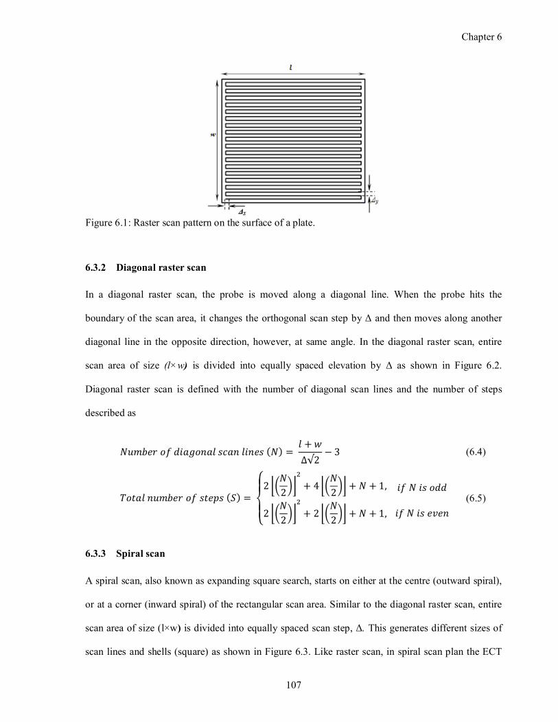
Chapter 6

107

6.3.2 Diagonal raster scan

In a diagonal raster scan, the probe is moved along a diagonal line. When the probe hits the

boundary of the scan area, it changes the orthogonal scan step by Δ and then moves along another

diagonal line in the opposite direction, however, at same angle. In the diagonal raster scan, entire

scan area of size (l×w) is divided into equally spaced elevation by Δ as shown in Figure 6.2.

Diagonal raster scan is defined with the number of diagonal scan lines and the number of steps

described as

������ �� �������� ���� ����� (�) = � + �

∆√2− 3 (6.4)

����� ������ �� ����� (�)=

⎩⎪⎨

⎪⎧

2 ���

2��

�

+ 4 ���

2�� + � + 1,

2 ���

2��

�

+ 2 ���

2�� + � + 1,

��� � �� ���

�� � �� ����

(6.5)

6.3.3 Spiral scan

A spiral scan, also known as expanding square search, starts on either at the centre (outward spiral),

or at a corner (inward spiral) of the rectangular scan area. Similar to the diagonal raster scan, entire

scan area of size (l×w) is divided into equally spaced scan step, Δ. This generates different sizes of

scan lines and shells (square) as shown in Figure 6.3. Like raster scan, in spiral scan plan the ECT

Figure 6.1: Raster scan pattern on the surface of a plate.

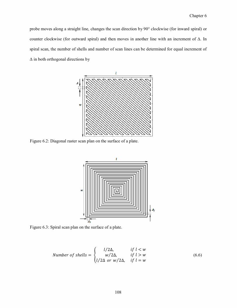
Chapter 6

108

probe moves along a straight line, changes the scan direction by 90° clockwise (for inward spiral) or

counter clockwise (for outward spiral) and then moves in another line with an increment of Δ. In

spiral scan, the number of shells and number of scan lines can be determined for equal increment of

Δ in both orthogonal directions by

������ �� �ℎ���� = �� 2∆⁄ , � 2∆,⁄

� 2∆⁄ �� � 2∆,⁄

�� � < � �� � > � �� � = �

� (6.6)

Figure 6.3: Spiral scan plan on the surface of a plate.

Figure 6.2: Diagonal raster scan plan on the surface of a plate.

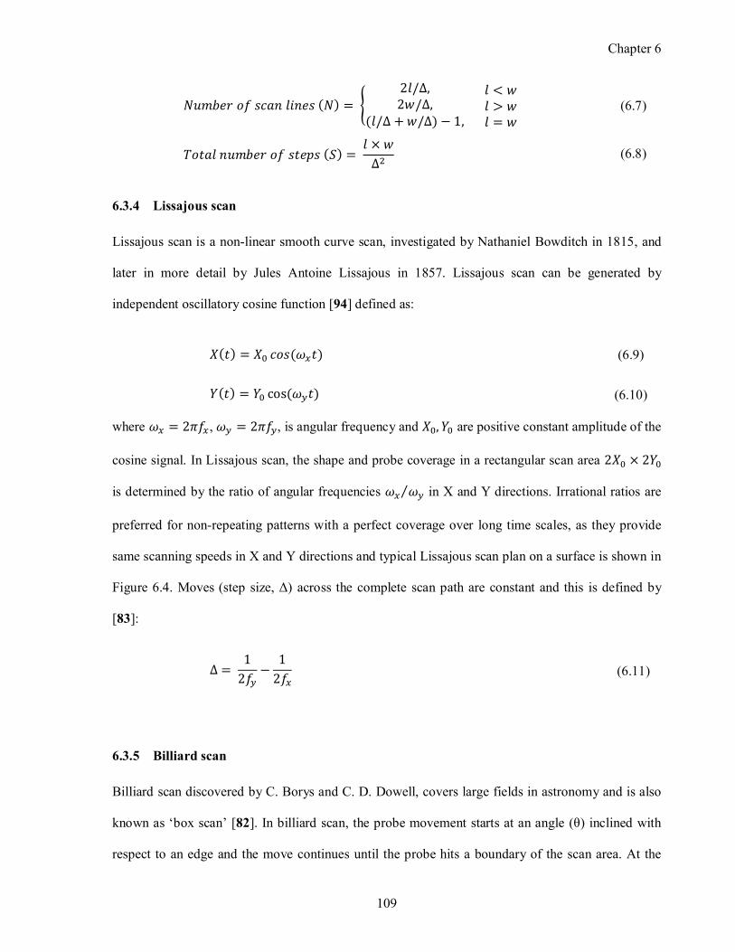
Chapter 6

109

������ �� ���� ����� (�) = �

2�/∆,2�/∆,

(�/∆ + �/∆)− 1,

� � < �� > �� = �

(6.7)

����� ������ �� ����� (�)= � × �

∆� (6.8)

6.3.4 Lissajous scan

Lissajous scan is a non­linear smooth curve scan, investigated by Nathaniel Bowditch in 1815, and

later in more detail by Jules Antoine Lissajous in 1857. Lissajous scan can be generated by

independent oscillatory cosine function [94] defined as:

�(�) = �� ���(���) (6.9)

�(�) = �� cos(���) (6.10)

where �� = 2��� , �� = 2���, is angular frequency and ��,�� are positive constant amplitude of the

cosine signal. In Lissajous scan, the shape and probe coverage in a rectangular scan area 2�� × 2��

is determined by the ratio of angular frequencies �� ��⁄ in X and Y directions. Irrational ratios are

preferred for non­repeating patterns with a perfect coverage over long time scales, as they provide

same scanning speeds in X and Y directions and typical Lissajous scan plan on a surface is shown in

Figure 6.4. Moves (step size, Δ) across the complete scan path are constant and this is defined by

[83]:

∆ = 1

2��−

1

2�� (6.11)

6.3.5 Billiard scan

Billiard scan discovered by C. Borys and C. D. Dowell, covers large fields in astronomy and is also

known as ‘box scan’ [82]. In billiard scan, the probe movement starts at an angle (θ) inclined with

respect to an edge and the move continues until the probe hits a boundary of the scan area. At the

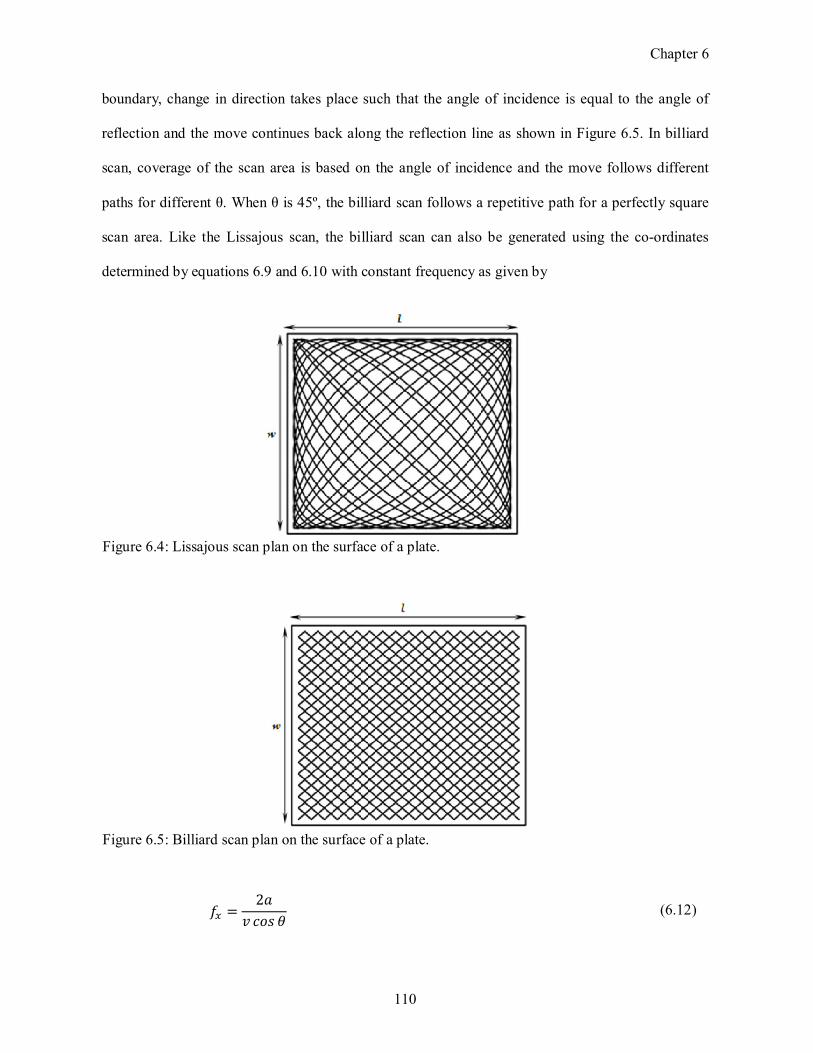
Chapter 6

110

boundary, change in direction takes place such that the angle of incidence is equal to the angle of

reflection and the move continues back along the reflection line as shown in Figure 6.5. In billiard

scan, coverage of the scan area is based on the angle of incidence and the move follows different

paths for different θ. When θ is 45º, the billiard scan follows a repetitive path for a perfectly square

scan area. Like the Lissajous scan, the billiard scan can also be generated using the co­ordinates

determined by equations 6.9 and 6.10 with constant frequency as given by

�� =2�

� ��� � (6.12)

Figure 6.5: Billiard scan plan on the surface of a plate.

Figure 6.4: Lissajous scan plan on the surface of a plate.

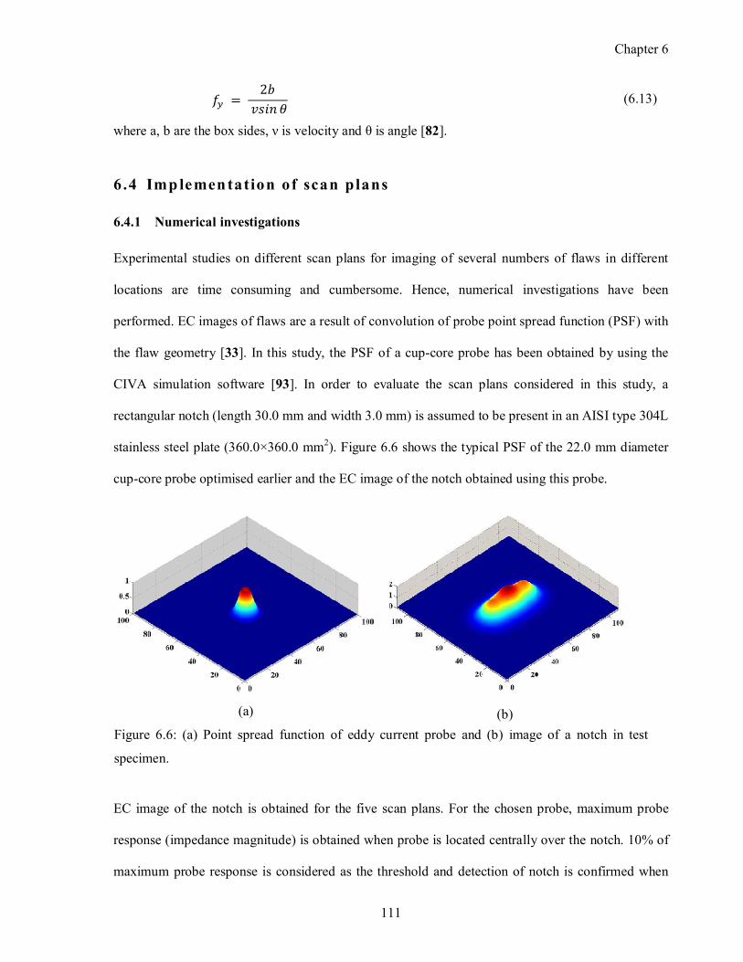
Chapter 6

111

�� = 2�

���� � (6.13)

where a, b are the box sides, ν is velocity and θ is angle [82].

6.4 Implementation of scan plans

6.4.1 Numerical investigations

Experimental studies on different scan plans for imaging of several numbers of flaws in different

locations are time consuming and cumbersome. Hence, numerical investigations have been

performed. EC images of flaws are a result of convolution of probe point spread function (PSF) with

the flaw geometry [33]. In this study, the PSF of a cup­core probe has been obtained by using the

CIVA simulation software [93]. In order to evaluate the scan plans considered in this study, a

rectangular notch (length 30.0 mm and width 3.0 mm) is assumed to be present in an AISI type 304L

stainless steel plate (360.0×360.0 mm2). Figure 6.6 shows the typical PSF of the 22.0 mm diameter

cup­core probe optimised earlier and the EC image of the notch obtained using this probe.

EC image of the notch is obtained for the five scan plans. For the chosen probe, maximum probe

response (impedance magnitude) is obtained when probe is located centrally over the notch. 10% of

maximum probe response is considered as the threshold and detection of notch is confirmed when

Figure 6.6: (a) Point spread function of eddy current probe and (b) image of a notch in test

specimen.

(b) (a)

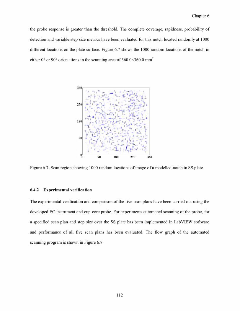
Chapter 6

112

the probe response is greater than the threshold. The complete coverage, rapidness, probability of

detection and variable step size metrics have been evaluated for this notch located randomly at 1000

different locations on the plate surface. Figure 6.7 shows the 1000 random locations of the notch in

either 0° or 90° orientations in the scanning area of 360.0×360.0 mm2

6.4.2 Experimental verification

The experimental verification and comparison of the five scan plans have been carried out using the

developed EC instrument and cup­core probe. For experiments automated scanning of the probe, for

a specified scan plan and step size over the SS plate has been implemented in LabVIEW software

and performance of all five scan plans has been evaluated. The flow graph of the automated

scanning program is shown in Figure 6.8.

Figure 6.7: Scan region showing 1000 random locations of image of a modelled notch in SS plate.

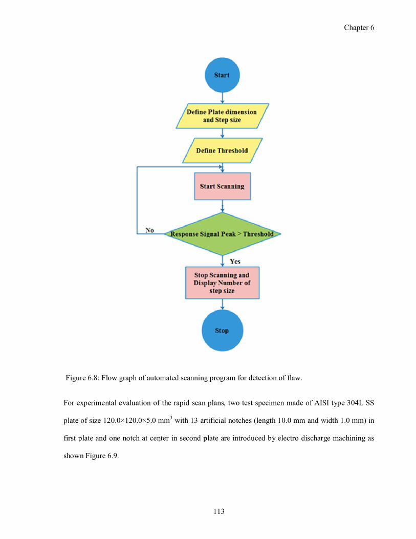
Chapter 6

113

For experimental evaluation of the rapid scan plans, two test specimen made of AISI type 304L SS

plate of size 120.0×120.0×5.0 mm3 with 13 artificial notches (length 10.0 mm and width 1.0 mm) in

first plate and one notch at center in second plate are introduced by electro discharge machining as

shown Figure 6.9.

Figure 6.8: Flow graph of automated scanning program for detection of flaw.

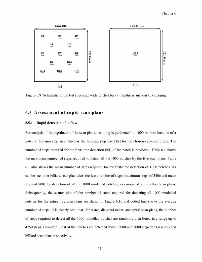
Chapter 6

114

6.5 Assessment of rapid scan plans

6.5.1 Rapid detection of a flaw

For analysis of the rapidness of the scan plans, scanning is performed on 1000 random location of a

notch at 5.0 mm step size which is the limiting step size [28] for the chosen cup­core probe. The

number of steps required for the first­time detection (hit) of the notch is predicted. Table 6.1 shows

the maximum number of steps required to detect all the 1000 notches by the five scan plans. Table

6.1 also shows the mean number of steps required for the first­time detection of 1000 notches. As

can be seen, the billiard scan plan takes the least number of steps (maximum steps of 3406 and mean

steps of 808) for detection of all the 1000 modelled notches, as compared to the other scan plans.

Subsequently, the scatter plot of the number of steps required for detecting all 1000 modelled

notches for the entire five scan plans are shown in Figure 6.10 and dotted line shows the average

number of steps. It is clearly seen that, for raster, diagonal raster, and spiral scan plans, the number

of steps required to detect all the 1000 modelled notches are randomly distributed in a range up to

4750 steps. However, most of the notches are detected within 3000 and 2000 steps for Lissajous and

billiard scan plans respectively.

Figure 6.9: Schematic of the test specimen with notches for (a) rapidness analysis (b) imaging.

(b) (a)

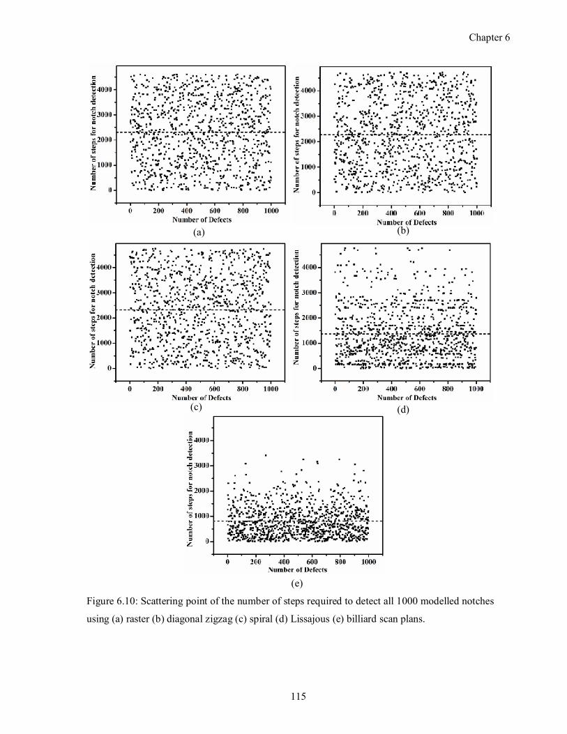
Chapter 6

115

(a) (b)

(c) (d)

(e)

Figure 6.10: Scattering point of the number of steps required to detect all 1000 modelled notches

using (a) raster (b) diagonal zigzag (c) spiral (d) Lissajous (e) billiard scan plans.

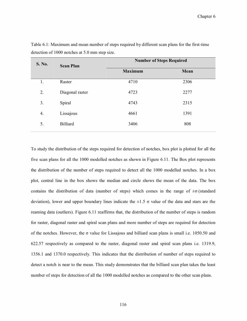
Chapter 6

116

Table 6.1: Maximum and mean number of steps required by different scan plans for the first­time

detection of 1000 notches at 5.0 mm step size.

S. No. Scan Plan Number of Steps Required

Maximum Mean

1. Raster 4710 2306

2. Diagonal raster 4723 2277

3. Spiral 4743 2315

4. Lissajous 4661 1391

5. Billiard 3406 808

To study the distribution of the steps required for detection of notches, box plot is plotted for all the

five scan plans for all the 1000 modelled notches as shown in Figure 6.11. The Box plot represents

the distribution of the number of steps required to detect all the 1000 modelled notches. In a box

plot, central line in the box shows the median and circle shows the mean of the data. The box

contains the distribution of data (number of steps) which comes in the range of ±σ (standard

deviation), lower and upper boundary lines indicate the ±1.5 σ value of the data and stars are the

reaming data (outliers). Figure 6.11 reaffirms that, the distribution of the number of steps is random

for raster, diagonal raster and spiral scan plans and more number of steps are required for detection

of the notches. However, the σ value for Lissajous and billiard scan plans is small i.e. 1050.50 and

622.57 respectively as compared to the raster, diagonal raster and spiral scan plans i.e. 1319.9,

1356.1 and 1370.0 respectively. This indicates that the distribution of number of steps required to

detect a notch is near to the mean. This study demonstrates that the billiard scan plan takes the least

number of steps for detection of all the 1000 modelled notches as compared to the other scan plans.

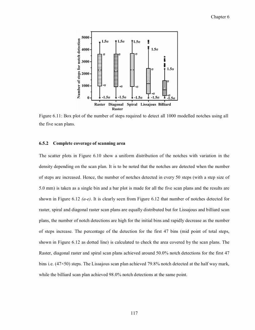
Chapter 6

117

6.5.2 Complete coverage of scanning area

The scatter plots in Figure 6.10 show a uniform distribution of the notches with variation in the

density depending on the scan plan. It is to be noted that the notches are detected when the number

of steps are increased. Hence, the number of notches detected in every 50 steps (with a step size of

5.0 mm) is taken as a single bin and a bar plot is made for all the five scan plans and the results are

shown in Figure 6.12 (a-e). It is clearly seen from Figure 6.12 that number of notches detected for

raster, spiral and diagonal raster scan plans are equally distributed but for Lissajous and billiard scan

plans, the number of notch detections are high for the initial bins and rapidly decrease as the number

of steps increase. The percentage of the detection for the first 47 bins (mid point of total steps,

shown in Figure 6.12 as dotted line) is calculated to check the area covered by the scan plans. The

Raster, diagonal raster and spiral scan plans achieved around 50.0% notch detections for the first 47

bins i.e. (47×50) steps. The Lissajous scan plan achieved 79.8% notch detected at the half way mark,

while the billiard scan plan achieved 98.0% notch detections at the same point.

Figure 6.11: Box plot of the number of steps required to detect all 1000 modelled notches using all

the five scan plans.

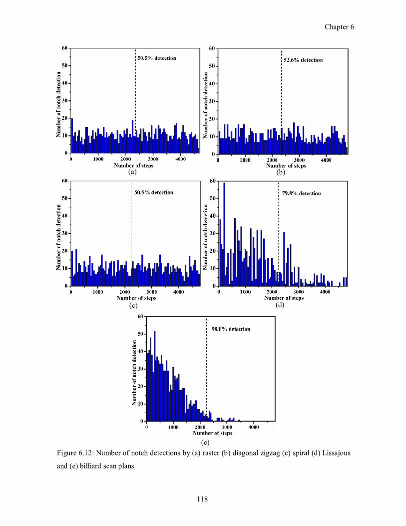
Chapter 6

118

(c) (d)

(b) (a)

(e)

Figure 6.12: Number of notch detections by (a) raster (b) diagonal zigzag (c) spiral (d) Lissajous

and (e) billiard scan plans.

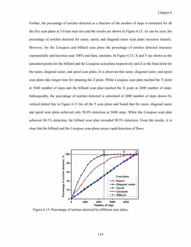
Chapter 6

119

Further, the percentage of notches detected as a function of the number of steps is estimated for all

the five scan plans at 5.0 mm step size and the results are shown in Figure 6.13. As can be seen, the

percentage of notches detected for raster, spiral, and diagonal raster scan plans increases linearly.

However, for the Lissajous and billiard scan plans the percentage of notches detected increases

exponentially and becomes near 100% and then, saturates. In Figure 6.13, X and Y are shown as the

saturation points for the billiard and the Lissajous scan plans respectively and Z as the final point for

the raster, diagonal raster, and spiral scan plans. It is observed that raster, diagonal raster, and spiral

scan plans take longer time for attaining the Z point. While Lissajous scan plan reached the Y point

at 3840 number of steps and the billiard scan plan reached the X point at 2400 number of steps.

Subsequently, the percentage of notches detected is calculated at 2400 number of steps shown by

vertical dotted line in Figure 6.13 for all the 5 scan plans and found that the raster, diagonal raster

and spiral scan plans achieved only 50.0% detection at 2400 steps. While the Lissajous scan plan

achieved 80.1% detection, the billiard scan plan recorded 98.5% detection. From the results, it is

clear that the billiard and the Lissajous scan plans ensure rapid detection of flaws.

Figure 6.13: Percentage of notches detected by different scan plans.

Chapter 6

120

6.5.3 Step size for detection of flaw

Systematic studies have been performed to investigate the influence of step size on flaw detection

for all the five scan plans. For this study, step sizes of 3.0 mm, 5.0 mm, 7.0 mm and 10.0 mm are

considered and the number of steps required for notch detection is calculated for all the five scan

plans. The resulting box plot is shown in Figure 6.14 (a-d). Table 6.2 and Table 6.3 show the mean

and standard deviation of the box plot for steps required for first time detection of notches

respectively. From the result, it is observed that the mean and standard deviation value for billiard

and Lissajous scan plans is less as compared to the raster, diagonal raster and spiral scan plans for all

step size i.e. 3.0, 5.0, 7.0 and 10.0 mm. However, as the step size increases the performance of

billiard and Lissajous scan plans decreases. However, the lower value of standard deviation shows

that the distribution of number of steps required to detect the notches is near to the mean. Hence,

from the result it is inferred that billiard and Lissajous scan plans perform faster as compared to the

raster, diagonal raster and spiral scan plans. In view of this, billiard and Lissajous scan plans are

selected for further investigations.

Table 6.2: Mean value of the number of steps required for first time detection of notches at

different step sizes.

Step size, mm Raster Diagonal

raster Spiral Lissajous Billiard

3.0 6210 6276 5894 3935 3538

5.0 2306 2277 2315 1391 808

7.0 1249 1228 1284 747 605

10.0 599 591 644 479 421

Chapter 6

121

Table 6.3: Standard deviation value of the number of steps required for first time detection of

notches at different step sizes.

Step size,

mm Raster

Diagonal

raster Spiral Lissajous Billiard

3.0 3684 3789 3940 3057 2683

5.0 1319 1356 1370 1050 622

7.0 681 699 681 586 474

10.0 335 340 333 356 304

(b)

(c)

Figure 6.14: Box plot of the number of steps required to detect all the 1000 modelled notches by

different scan plans at a step size of (a) 3.0 mm (b) 5.0 mm (c) 7.0 mm and (c) 10.0 mm.

(d)

(a)

Chapter 6

122

6.6 Bill iard scan plan

6.6.1 Influence of notch location

For understanding the area coverage and notches missed during the scan, studies are carried out

using Lissajous and the billiard scan plans. Figure 6.15 (a) shows the Lissajous scan plan with an

overlay of location of undetected notches. As can be seen, the Lissajous scan plan spends longer

time on the edges relative to the center of the pattern. However, the billiard scan plan covers

uniformly across the entire scan area as shown in Figure 6.15 (b) and detects the notches including

those missed by the Lissajous scan plan. This study demonstrates that although the Lissajous scan

plan is rapid, there is a possibility that some of flaws present in the central regions of object would

be missed. This reaffirms that the billiard scan plan ensures full uniform coverage with rapidness

and 100% POD.

6.6.2 Influence of notch dimensions

The length of notch is important for detection by ECT technique. To study the effect of notch length

on billiard and Lissajous scan plans, three notches of different lengths 10.0, 20.0 and 30.0 mm are

(a) Figure 6.15: Missing location of notches in modelled test specimen and coverage of the scan plans

(a) Lissajous (b) billiard.

(b)

Chapter 6

123

modelled and percentage of notches detected is estimated at 5.0 mm step size. As seen in Figure

6.16, as the notch length increases the percentage of notches detected for 1000 random notch

location increases for both the Lissajous and the billiard scan plans. Points X, Y and Z are the

saturation points for notch lengths 10.0, 20.0 and 30.0 mm respectively for the billiard scan plan.

The number of steps for saturation decreases with increase in notch length for the billiard scan plan.

The percentage of notches detected is higher for the billiard scan plan as compared to the Lissajous

scan plan for all the three lengths. Hence, the billiard scan plan is suitable for detection of short

length notches i.e. 10.0 mm length.

6.6.3 Influence of angle of incidence

Initial angle of incidence (θ) is important for the billiard scan plan. A systematic study has been

carried out to analyse this. For selection of the optimum angle of incidence for the billiard scan plan,

different angle viz. 5 ,̊ 15 ,̊ 25 ,̊ 35 ̊and 44 ̊are chosen and analysis is performed by scanning the

1000 modelled location of notches at 5.0 mm step size. Percentage of notches detected for these

angles are calculated and the results are shown in Figure 6.17. It is clearly seen that for 2400 scan

steps (dotted line shown in Figure 6.17), the percentage of notch detection is 80.0%, 93.0%, 95.0% ,

(a) (b) Figure 6.16: Detection of notches with different length of notches for (a) Lissajous scan plan

(b) billiard scan plan.

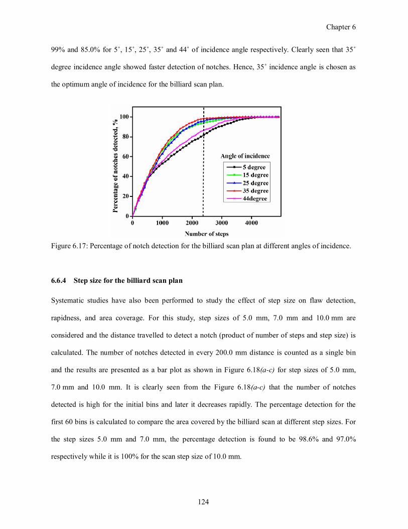
Chapter 6

124

99% and 85.0% for 5 ,̊ 15 ,̊ 25 ,̊ 35 ̊and 44 ̊of incidence angle respectively. Clearly seen that 35˚

degree incidence angle showed faster detection of notches. Hence, 35 ̊incidence angle is chosen as

the optimum angle of incidence for the billiard scan plan.

6.6.4 Step size for the billiard scan plan

Systematic studies have also been performed to study the effect of step size on flaw detection,

rapidness, and area coverage. For this study, step sizes of 5.0 mm, 7.0 mm and 10.0 mm are

considered and the distance travelled to detect a notch (product of number of steps and step size) is

calculated. The number of notches detected in every 200.0 mm distance is counted as a single bin

and the results are presented as a bar plot as shown in Figure 6.18(a-c) for step sizes of 5.0 mm,

7.0 mm and 10.0 mm. It is clearly seen from the Figure 6.18(a-c) that the number of notches

detected is high for the initial bins and later it decreases rapidly. The percentage detection for the

first 60 bins is calculated to compare the area covered by the billiard scan at different step sizes. For

the step sizes 5.0 mm and 7.0 mm, the percentage detection is found to be 98.6% and 97.0%

respectively while it is 100% for the scan step size of 10.0 mm.

Figure 6.17: Percentage of notch detection for the billiard scan plan at different angles of incidence.

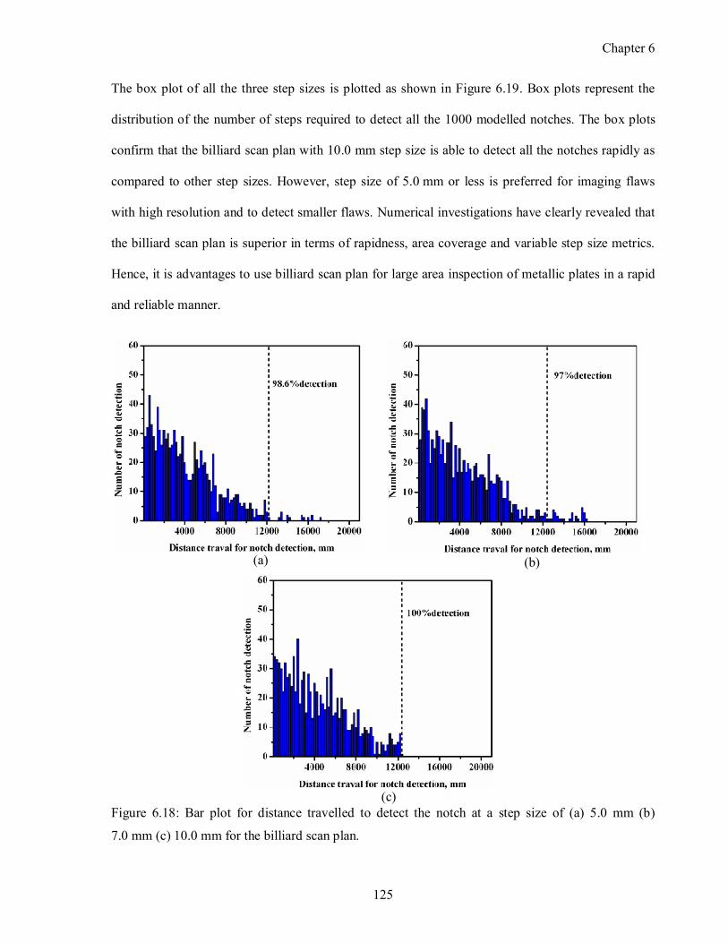
Chapter 6

125

The box plot of all the three step sizes is plotted as shown in Figure 6.19. Box plots represent the

distribution of the number of steps required to detect all the 1000 modelled notches. The box plots

confirm that the billiard scan plan with 10.0 mm step size is able to detect all the notches rapidly as

compared to other step sizes. However, step size of 5.0 mm or less is preferred for imaging flaws

with high resolution and to detect smaller flaws. Numerical investigations have clearly revealed that

the billiard scan plan is superior in terms of rapidness, area coverage and variable step size metrics.

Hence, it is advantages to use billiard scan plan for large area inspection of metallic plates in a rapid

and reliable manner.

(b)

(c) Figure 6.18: Bar plot for distance travelled to detect the notch at a step size of (a) 5.0 mm (b)

7.0 mm (c) 10.0 mm for the billiard scan plan.

(a)

Chapter 6

126

6.7 Experimental verification of the Bill iard scan plan

In order to check the performance of the scan plans, a series of experiments are carried out on two

test specimens shown in Figure 6.9. The number of steps required to detect all the 13 notches (as

given in Figure 6.9 (a)) for the first time is calculated for all the five scan plans. Figure 6.20 shows

the box plot of steps required to detect all the 13 notches. From the figure it is clearly seen that for

the billiard scan plan, distribution of number of steps required to detects the notches is near to the

mean, due to the small value of σ (38.6) as compared to the raster, diagonal raster, spiral and

Lissajous (128.5, 126.1, 126.8 and 52.1 respectively) scan plans. The details of number of steps

required to detect the notches are shown in Table 6.4. From the result, it is clear that the number of

steps required to detect the notches depends on the notch location for all the five scan plans.

However, billiard scan plan performed faster as compared to other scan plans. It takes a maximum of

122 steps to detect all the 13 notches present in the SS plate. A very good agreement is seen between

the numerical and experimental results.

Figure 6.19: The box plot for distance travelled to detect the notch at different step sizes by the

billiard scan plan.

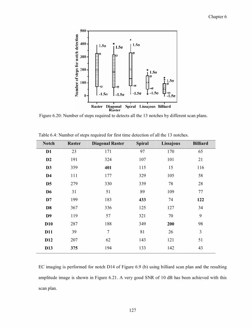
Chapter 6

127

Table 6.4: Number of steps required for first time detection of all the 13 notches.

Notch Raster Diagonal Raster Spiral Lissajous Billiard

D1 23 171 97 170 65

D2 191 324 107 101 21

D3 359 401 115 15 116

D4 111 177 329 105 58

D5 279 330 339 78 28

D6 31 51 89 109 77

D7 199 183 433 74 122

D8 367 336 125 127 34

D9 119 57 321 70 9

D10 287 188 349 200 98

D11 39 7 81 26 3

D12 207 62 143 121 51

D13 375 194 133 142 43

EC imaging is performed for notch D14 of Figure 6.9 (b) using billiard scan plan and the resulting

amplitude image is shown in Figure 6.21. A very good SNR of 10 dB has been achieved with this

scan plan.

Figure 6.20: Number of steps required to detects all the 13 notches by different scan plans.

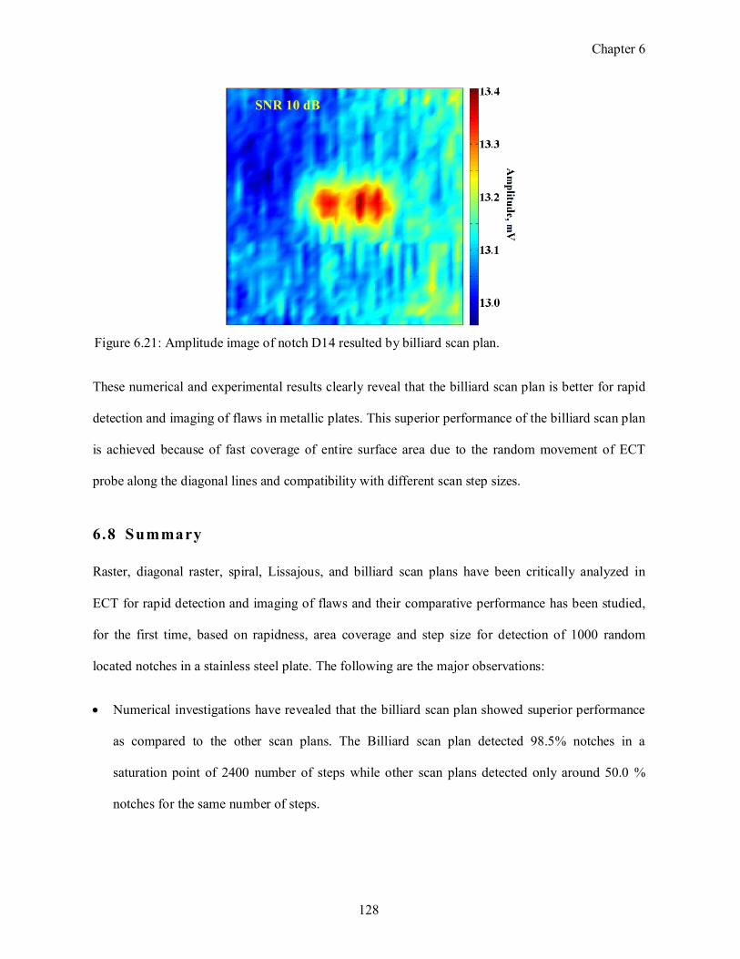
Chapter 6

128

These numerical and experimental results clearly reveal that the billiard scan plan is better for rapid

detection and imaging of flaws in metallic plates. This superior performance of the billiard scan plan

is achieved because of fast coverage of entire surface area due to the random movement of ECT

probe along the diagonal lines and compatibility with different scan step sizes.

6.8 Summary

Raster, diagonal raster, spiral, Lissajous, and billiard scan plans have been critically analyzed in

ECT for rapid detection and imaging of flaws and their comparative performance has been studied,

for the first time, based on rapidness, area coverage and step size for detection of 1000 random

located notches in a stainless steel plate. The following are the major observations:

Numerical investigations have revealed that the billiard scan plan showed superior performance

as compared to the other scan plans. The Billiard scan plan detected 98.5% notches in a

saturation point of 2400 number of steps while other scan plans detected only around 50.0 %

notches for the same number of steps.

SNR 10 dB

Figure 6.21: Amplitude image of notch D14 resulted by billiard scan plan.

Chapter 6

129

Studies revealed that 35 ̊ is optimum angle of incidence for the billiard scan plan for rapid

detection of notches in a square region of imaging. The billiard scan plan performance did not

degrade when the step size was doubled to 10.0 mm.

The study establishes, for the first time, that the billiard scan plan is an alternate scan plan to

raster scan for rapid and reliable inspection of large surfaces of electrically conducting materials

by ECT.

The performance of the billiard scan plan has also been experimentally verified on a 5.0 mm

thick stainless steel plate having a notch. The EC image obtained by billiard scan plan was found

to have an SNR of 10 dB.

The study proposes the use of billiard scan plan for rapid and reliable inspection of large surfaces

of electrically conducting material surfaces during ECT either during quality assurance or in­

service inspection.

130

Conclus ion and Future works

7.1 Conclusion

The thesis has focused on the development of eddy current methodologies for rapid and reliable

detection and imaging of sub­surface flaws in metallic materials. The thesis has extensively

demonstrated the possible methodologies for detection of sub­surface flaws in austenitic stainless

steel.

Developmental studies on the enhancement of sub­surface flaws detection have been carried out to

overcome the limitation of the conventional ECT. The conventional ECT is, in general, confined to

detection of sub­surface flaws within 5.0 mm depth in stainless steel plates. Detection of flaws in

thicker plate in range of 8.0 mm to 12.0 mm, such as storage tanks in nuclear reprocessing plants

made by the 304L austenitic stainless steel is essential. Hence, for reliable and rapid detection and

imaging of sub­surface flaws in 12.0 mm thick austenitic stainless steel, the thesis has proposed for

the first time four effective eddy current methodologies. These methodologies include development

of a high throughput probe, a high sensitive instrument, a novel fusion methodology and rapid

imaging scan plan. The major conclusions of the thesis and future work are given below.

Finite element modelling studies have been carried out using COMSOL multi­physics software

for selection of optimum coil probe configuration among send­receive type air core, ferrite core,

ferrite core with outer shielding and cup­core probes. The performance of these four types of

probe has been analysed based on predicted parameters viz., magnetic flux density (indicative of

low reluctance path), eddy current density (indicative of flux concentration at flaw location) and

change in phase angle (indicative of detection sensitivity in depth direction). Model predictions

reveal that cup­core probe produces higher magnetic flux density, eddy current density and

7

Chapter 7

131

change in phase angle for flaws located at more than 5.0 mm below the surface as compared to

other probe configurations. Model prediction and experimental studies confirm that the optimum

diameter and excitation frequency are 22.0 mm and 5 kHz for detection of sub­surface flaw in

12.0 mm thick austenitic stainless steel plates.

A high sensitive eddy current instrument consisting of a high current sinusoidal driving unit and

a digital lock­in amplifier based precise measurement unit has been designed and developed. The

digital lock­in amplifier is capable of precisely measuring the phase lag (sensitivity,

0.001 degree) of the sinusoid from flaw regions using I/Q detection technique which is

implemented using LabVIEW software. Systematic studies using this instrument revealed a

definite improvement in the detection sensitivity with increase in excitation current and by use of

precise phase angle measurement. For AISI 304L stainless steel plate of thickness 12.0 mm, an

increase in phase angle is observed with increase in the excitation current up to 550 mA and

ensured reliable detection of a sub­surface notch located 8.0 mm below the surface.

From the experimental results it is also observed that, the cup­core probe and instrument produce

a linear relationship between the flaw location below the surface and change in phase angle. This

linear relationship facilitates improvement in detection and sizing of deep sub­surface flaws with

better resolution in depth direction. It is found that the instrument and cup­core type send­receive

probe enable identification of surface and sub­surface flaws because the change in sign of the

phase angle signals.

A novel BayWT based image fusion methodology is proposed to further enhance the capability

of the instrument and optimised probe to image sub­surface flaws. BayWT based image fusion is

an integrated fusion methodology of wavelet transform and Bayesian fusion method. BayWT

based fusion method has shown significant improvement in SNR as compared to the other fusion

method viz. Laplacian pyramid, wavelet transformed, principal component analysis and

Bayesian method. BayWT based fusion method achieved an SNR of 17.63 dB, which is three

Chapter 7

132

times the SNR of the input images (5.36 dB) and a 7.0 dB more than achieved by other fusion

methods (10.0 dB).

For automated ECT of large size austenitic stainless steel components in radioactive

environment, different type of scan plans such as raster, diagonal raster, spiral, Lissajous and

billiard have been studied, for the first time. The comparative performance has been studied

based on rapidness, area coverage and variable step size metrics for selection of rapid scan plan,

after scanning of 1000 random located notch in a stainless steel plate. The billiard scan plan has

been found to be 2 times faster than that of the other scan plans and showed superior

performance as compared to other scan plans. Studies revealed that 35 degree is optimum angle

of incidence for the billiard scan plan for rapid detection of notches. The performance of the

billiard scan plan did not degrade when the step size was doubled to 10.0 mm. Thus, the study

establishes, for the first time, that the billiard scan plan is an alternate scan plan to the traditional

raster scan for rapid and reliable detection and imaging of large surface of electrically conducting

materials by eddy current testing.

7.1.1 Technical and scientific contributions

The major contributions of this thesis for detection of sub­surface flaws in metallic materials are the

following:

A high throughput send­receive type cup­core coil probe has been designed and developed

for ensuring deeper penetration of eddy currents into the material. This probe has shown

higher sensitivity for surface as well sub­surface flaws in 12.0 mm thick austenitic stainless

steel plates.

An eddy current instrument capable for generation of high excitation current and precisely

measuring the phase using a digital lock­in amplifier implemented in LabVIEW software has

Chapter 7

133

been designed and developed. This instrument can be used for detection of sub­surface flaws

as well as surface flaws in any metallic material.

For enhancement of the eddy current images of sub­surface flaws, a novel BayWT image

fusion methodology has been developed combining the capabilities of wavelet transform and

Bayesian method. This fusion method has resulted in a very high SNR of 17.63 dB. This

methodology can be readily extended to ultrasonic, radiography and thermography images

for enhanced detection of flaws and for their accurate sizing.

For reduction of radiation dose to the inspection personnel, billiard scan plan has been proposed

for the first time as a rapid scan plan for eddy current imaging of flaws. The proposed scan

plan is expected to change the way ECT imaging is carried out in future.

The methodologies developed in the thesis are expected to ensure faster eddy current

imaging inspection of storage tanks of reprocessing plants of FBR.

7.2 Future works

The works presented in this thesis has significantly improved the capability for detection of deep

sub­surface flaws in thick stainless steel components. In this thesis, high sensitive eddy current

instrument, high throughput send­receive type cup­core coil probe and BayWT based fusion have

been developed and they demonstrated better detection sensitivity for sub­surface flaws located

8.0 mm below the surface. Embedded flaws are not considered in the present study. It may be worth

exploring the instrument and probe developed for detection of corrosion in second and third layer of

aircraft structures.

In the FE model, relative permeability �� is assumed to be constant for ferrite core and shielding as

the excitation frequency are < 100 kHz. However at higher frequency, it is essential to consider non­

linear magnetisation components in the model for obtaining accurate results.

Chapter 7

134

In the present study, flaw depth and location are considered for selection of the probe configuration.

However, more information can be obtained by detailed modelling studies at varying surface

conditions, probe tilt and varying lift­off, towards fine tuning the instrument and probe performance

and to explore other possible signal and image processing methods.

For optimisation of the probe configuration, a 2D­axi­symmetric model is used. These model

predictions are sufficient to optimise probe and frequency, does not consider the flaw orientation.

For this purpose and also to model other 3­dimensional situations such as non­uniform

electromagnetic coupling three dimensional (3D) model investigation is essential.

In this thesis, an optimum probe diameter has been found as 22.0 mm for AISI 304L stainless steel

plate of thickness 12.0 mm. For other thicknesses, optimum diameter and excitation frequency will

change. Hence, it may be beneficial to investigate further and establish a relationship among probe

diameter, frequency and thickness for better applicability of the cup­core type send­receive probe for

various applications and for generalisation purpose.

In this thesis, the synergistic combination of probe and instrument clearly ensured detection of inside

corrosion damage upto 12.0 mm thick stainless steel storage tanks by scanning the probe on the

outer surface. Further works may be interesting to use the instrument and probe to detect corrosion

damage present in actual storage tanks or through accelerated corrosion studies. It will also be

beneficial to evaluate the sensitivity of the instrument and probe for different object geometries and

in different materials. Detection of flaws of length 30.0 mm has been studied in this thesis. It may be

worth studying the instrument sensitivity and capability to detect shorter flaws.

In this study curvature surface of the vessels is analysed as plate due to the large diameter of the

vessels (~10 m) curvature effect are ignored. It will be useful to test the probe on actual components

and design suitable curved front face to minimize coupling issues.

Chapter 7

135

For the envisaged detection of inside surface corrosion electromagnetic acoustic transducers

(EMATs) probes, capable of performing both ultrasonic and eddy current testing, may be studied for

detection of sub­surface flaws.

The optical images are usually sharp as the optical sources posses point delta function. While the

eddy current images are blurred (over sized) as the probes are of finite size and have a point spread

function that is circular and like a 2D­ Gaussian function. When a fusion methodology is applied,

more enhancements are likely for the optical images as compared to eddy current images. However,

more detailed studies are required to compare and make a quantitative assessment.

Flaws orientation of 0 and 90 degree is used for evaluation of the rapid scan plans. Studies on

detection of notches at different orientations are worth to check the performance of the billiard scan

plan. This work can be extended by studying the performance of the scan plans using different types

of probes such as absolute, differential etc towards identifying much better probe type and

configuration for detection of flaws in thick material.

136

References

[1] D. E. Bray and R. K. Stanley, Non-destructive evaluation: a tool for design, manufacturing, and service.: McGraw­Hill, 1989.

[2] Charles J. Hellier, Handbook of non-destructive evaluation.: McGraw­Hill, 2013.

[3] B. P. C. Rao, Practical eddy current testing. New Delhi: Narosa Publishing House, 2007.

[4] Farhad Tovassoli, Advances in stainless steel, Baldev Raj, Ed.: Universities Press, 2010.

[5] Baldev Raj, T. Jayakumar, and M. Thavasimuthu, Practical non-destructive testing, 3rd ed. New Delhi: Narosa Publishing House, 2007.

[6] P. J. Shull, Non-destructive evaluation: theory, techniques and applications. New York: Marcel Dekkar Inc., 2002.

[7] H. L. Libby, Introduction to electromagnetic NDT methods. New York: Wiley Interscience, 1971.

[8] B. P. C. Rao, "Eddy Current T esting: Basics," Journal of Non Destructive T esting \& Evaluation, vol. 10, pp. 7­16, 2011.

[9] S. S. Udpa and Patrick O Moore, Nondestructive Testing Handbook Third Edition. Volume 5 Electromagnetic.: Testing,American Society of Nondestructive Testing, 2004.

[10] N. Ida, Numerical modeling for electromagnetic Non-destructive evaluation.: Chapman and Hall, 1995.

[11] Lalita Udpa, "Imaging of electromagnetic NDT phenomena," Colorado State University, Ph.D. dissertation 1986.

[12] R. McCary, D. Oliver, K. Silverstein, and J. Young, "Eddy current imaging," IEEE Transactions on Magnetics, vol. 20, no. 5, pp. 1986­1988, 1984.

[13] R. Joynson, R. McCary, D. Oliver, K. Silverstein­Hedengren, and L. Thumhart, "Eddy current imaging of surface­breaking structures," IEEE Transactions on Magnetics, vol. 22, no. 5, pp. 1260­1262, 1986.

[14] Baldev Raj, U. Kamachi Mudali, T. Jayakumar, K. V. Kashiviswanathan, and R. Natarajan, "Meeting the challenges related to material issues in chemical industries," Sadhana, vol. 25, no. 6, pp. 519­559, December 2000.

[15] Baldev Raj and U. Kamachi Mudali, "Materials development and corrosion problems in nuclear fuel reprocessing plants," Progress in Nuclear Energy, vol. 48, no. 4, pp. 283–313, 2006.

[16] C. V. Dodd and W. E. Deeds, "Analytical Solutions to Eddy­Current Probe­Coil Problems," Journal of Applied Physics, vol. 39, no. 6, pp. 2829­2838, May 1968.

[17] Z. Mottl, "The quantitative relations between true and standard depth of penetration for air­cored probe coils in eddy current testing," NDT International, vol. 23, no. 1, pp. 11­18, 1990.

137

[18] G. Mook, O. Hesse, and V. Uchanin, "Deep Penetrating Eddy Currents and Probes," MP Materials Testing, vol. 49, pp. 258­264, 2007.

[19] (2001­2012) NDT Education Resource Center, The collaboration for NDT education. [Online]. http://www.ndt­ed.org

[20] S. Thirunavukkarasu, B. P. C. Rao, T. Jayakumar, and Baldev Raj, "Techniques for processing remote field eddy current signals from bend regions of steam generator tubes of prototype fast breeder reactor," Annals of Nuclear Energy, vol. 38, pp. 817­824, 2011.

[21] P. Xiang, S. Ramakrishnan, X. Cai, P. Ramuhalli, R. Polikar, S. S. Udpa, and L. Udpa, "Automated analysis of rotating probe multi­frequency eddy current data from steam generator tubes," International Journal of Applied Electromagnetics and Mechanics, vol. 12, pp. 151­164, 2000.

[22] B. Sasi, Cacciola Matteo, C. Babu Rao, T. Jayakumar, and Baldev Raj, "Hybrid Signal Processing Approach for Enhanced Detection of Defects in EC­NDE," Research in Nondestructive Evaluation, vol. 24, pp. 51–61, 2013.

[23] B. P. C. Rao, Baldev Raj, T. Jayakumar, and P. Kalyanasundaram, "An intelligent imaging scheme for automated eddy current testing," Nondestructive Testing and Evaluation, vol. 17, no. 1, pp. 41­57, 2001.

[24] B. Sasi, Matteo Cacciola, Lalita Udpa, B. P. C. Rao, T. Jayakumar, and Baldev Raj, "Development of image fusion methodology using discrete wavelet transform for eddy current images," NDT & E International, vol. 51, pp. 51­57, 2012.

[25] X. E. Gros, P. Strachan, D. W. Lowden, and I. Edwards, "NDT data fusion," in in Proc. 6th Eur. Conf. Nondestructive Testing, 1994, pp. 355–359.

[26] R. Prachetaa and B. P. C. Rao, "Image Processing for NDT images," in IEEE International Conference on Signal and Image Processing (ICSIP), 2010, pp. 169­174.

[27] P. J. Burt and E.H. Adelson, "The Laplacian pyramid as a compact image code," IEEE Transactions on Communications, vol. 31, no. 4, pp. 432­540, 1983.

[28] S. Shuaib Ahmed, "Machine learning based inversion studies in eddy current non­destructive evaluation," HBNI Mumbai, PhD dissertation 2014.

[29] V.P.S. Naidu and J.R. Rao, "Pixel­level Image Fusion using Wavelets and Principal Component Analysis," Defence Science Journal, vol. 58, no. 3, pp. 338­352, 2008.

[30] Patrick J. Van Fleet, Discrete wavelet transformations: An elementary approach with applications.: A John wiley & Sons, 2007.

[31] Ali Mohammad­Djafari, "A Full Bayesian Approach for Inverse Problems," in Maximum Entropy and Bayesian Methods, KennethM. and Silver, RichardN. Hanson, Ed.: Springer Netherlands, 1996, pp. 135­144.

[32] A. M. Djafari, "A Bayesian approach for data and image fusion," in 22nd International Workshop on Bayesian Inference and Maximum Entropy Methods in Science and Engineering. AIP Conference Proceedings, vol. 659, 2003, pp. 386­408.

[33] S. Thirunavukkarasu, B. P. C. Rao, Anil Kumar Soni, S. Shuaib Ahmed, and T. Jayakumar, "Comparative performance of image fusion methodologies in eddy current testing,"

138

Research Journal of Applied Sciences, Engineering and Technology, vol. 4, no. 24, pp. 5548­5551, 2012.

[34] A. Lopes Ribeiro and H. Geirinhas Ramos, "Inductive probe for flaw detection in non­magnetic metallic plates using eddy currents," , vol. 12, 2008, pp. 1447­1451.

[35] D. G. Park, C. S. Angani, G. D. Kim, C. G. Kim, and Y. M. Cheong, "Evaluation of Pulsed Eddy Current Response and Detection of the Thickness Variation in the Stainless Steel," IEEE Transactions on Magnetics, vol. 45, no. 10, pp. 3893­3896, 2009.

[36] Y. He, F. Luo, M. Pan, X. Hu, J. Gao, and Bo. Liu, "Defect Classification based on rectangular pulsed eddy current sensor in different directions," Sensors and Actuators A: Physical, vol. 157, no. 1, pp. 26­31, 2010.

[37] D. Roy, R. Chakroborty, and B. K. Kaushik, "Comparative study of E­shaped coil and evolution of new methodology for crack detection using eddy current testing," Insight- Non-Destructive Testing and Condition Monitoring, vol. 55, no. 10, pp. 553­557, 2013.

[38] Eric Vourc’h, Pierre­Yves Joubert, Guillaume Le Gac, and Pascal larzabal, "Nondestructive evaluation of loose assemblies using multi­frequency eddy currents and artificial neural networks," Measurement Science and Technology, vol. 24, p. 125604, 2013.

[39] D. Placko and I. Dufour, "A focused­field eddy current sensor for nondestructive testing," IEEE Transactions on Magnetics, vol. 29, no. 6, pp. 3192­3194, 1993.

[40] K Arunachalam, L. Udpa, and S. Udpa, "Statistical analysis of array probe eddy current data from steam generator tubes," Studies in Applied Electromagnetics and Mechanics, vol. 36, pp. 159­166, 2012.

[41] J. Xin, L. Udpa, S. Udpa, R. Grimberg, and A Savin, "Rotating field eddy current probe for cylindrical samples," Studies in Applied Electromagnetics and Mechanics, vol. 39, pp. 60­74, 2014.

[42] P. Palanisamy and K. M. Lakin, "Development of EC inspection technique for sleeved engine disk bolt holes," Review of Progress in Quantitative Non-destructive Evaluation, vol. 2A, pp. 205­223, 1983.

[43] H. Hoshikawa, R. M. Li, and N. Ida, "Finite element analysis of eddy current surface probes," Review of Progress in Quantitative Nondestructive Evaluation, vol. 3A, pp. 675­682, 1984.

[44] Shin Young, Kil Choi, and Dong Myung, "Design of a Shielded Reflection Type Pulsed Eddy Current Probe for the Evaluation of Thickness," Journal of the Korean Society for Nondestructive Testing, vol. 27, no. 5, pp. 398­408, 2007.

[45] B. Sasi, B. P. C. Rao, S. Thirunavukkarasu, T. Jayakumar, and Baldev Raj, "Eddy Current­Giant Magneto­Resistive (GMR) Sensor for Nondestructive Detection of Deep­surface Defects," in Conference Proc. of 12th National seminar on Physics and Technology of Sensors, vol. 1, 2007.

[46] C. S. Angani, D. G. Park, C. G. Kim, P. Leela, M. Kishore, and Y. M. Cheong, "Pulsed eddy current differential probe to detect the defects in a stainless steel pipe," Journal of Applied Physics, vol. 109, no. 7, p. 07D348, 2011.

139

[47] C. Claeys and E. Simon, Radiation effects in advanced semiconductor materials and devices.: Springer Series in Material Science, 2002.

[48] T. P. Theodoulidis, "Model of ferrite­cored probes for eddy current nondestructive evaluation," Journal of applied physics, vol. 91, no. 53, pp. 3071­3078, 2003.

[49] M. Cacciola, G. Megali, D. Pellicanµo, S. Calcagno, M. Versaci, and F. C. Morabito, "Modelling and Validating Ferrite­core Probes for GMR­eddy Current Testing in Metallic Plates," PIERS online, vol. 6, no. 3, pp. 237­241, 2010.

[50] Z. Zeng, Lalita Udpa, and S. S. Udpa, "Finite­Element Model for simulation of ferrite­core eddy­current probe," IEEE Transactions on Magnetics, vol. 46, no. 3, pp. 905­909, 2010.

[51] S.N. Vernon and T.A.O. Gross, "Effects of Shielding on Properties of Eddy Current Probes with Ferrite Cup Cores," in Review of Progress in Quantitative Nondestructive Evaluation, Donald O. Thompson and Dale E. Chimenti, Eds.: Springer US, 1987, vol. 6 A, pp. 713­719. [Online]. http://dx.doi.org/10.1007/978­1­4613­1893­4_80

[52] P. Y. Joubert, E. Vourc’h, Tassin, A. Diraison, and Y. Le, "Source separation techniques applied to the detection of subsurface defects in the eddy current NDT of aeronautical lap­joints," NDT& E International, vol. 43, no. 7, pp. 606­614, 2010. [Online]. http://www.sciencedirect.com/science/article/pii/S096386951000071X

[53] A. J. Bahl and D. W. Cooley, "Analysis and Design of Eddy­Current Measurement Systems," Review of Progress in Quantitative Nondestructive Evaluation, vol. 2A, pp. 225­244, 1983.

[54] T. E. Capobianco and F. R. Fickett, "Precision Measurement of Eddy Current Coil Parameters," Review of Progress in Quantitative Nondestructive Evaluation, vol. 4A, pp. 491­498, 1985.

[55] J. Blitz, "Nondestructive testing using electromagnetic instrumentation," Journal of Physics E: Scientific Instruments, vol. 16, p. 1135, 1983.

[56] Dario Pasadas, T. Jorge Rocha, Helena Geirinhas Ramos, and A. Lopes Ribeiro, "Evaluation of portable ECT instruments with positioning capability," Measurement, vol. 45, pp. 393­404, 2012.

[57] Wang Chao, Zhi Ya, and Gao Peng, "GMR based eddy current system for defect detection," in Proceedings of the 11th IEEE International Conference on Electronic Measurement \& Instruments, 2013.

[58] Naveen V. Nair, Vikram R. Melapudi, Hector R. Jimenez, Xin Liu, Yiming Deng, Zhiwei Zeng, Lalita Udpa, Thomas J. Moran, and S. S. Udpa, "A GMR­Based Eddy Current System for NDE of Aircraft Structures," IEEE Transactions on Magnetics, vol. 42, no. 10, pp. 3312­3314, 2006.

[59] P. Clarkson, T. J. Esward, P. M. Harris, A. A. Smith, and I. M. Smith, "Software simulation of a lock­in amplifier with application to the evaluation of uncertainties in real measuring systems," Measurement Science and Technology, vol. 21, pp. 45106­45116, 2010.

[60] P. G. Doctor, T. P. Harington, T. J. Davis, C. J. Morris, and D. W. Farley, Pattern recognition methods for classifying and sizing flaws using eddy current data, G. Birnbaum and G. Free, Eds.: ASTM STP­ 722, 1981.

140

[61] S. S. Udpa and W. Lord, "Fourier descriptors classification scheme for differential probe signal," Material evaluation, vol. 42, pp. 1136­1141, 1984.

[62] M. T. Shyamsunder, C. Rajgopalan, Baldev Raj, S. K. Dewangan, B. P. C. Rao, and K. K. Ray, "Pattern recognition approaches for detection and characterization of defects by eddy current testing," Materials Evaluation, vol. 51, no. 1, pp. 93­101, 2000.

[63] P. Kalyanasundaram, S. Thirunavukkarasu, B. P. C. Rao, T. Jayakumar, and Baldev Raj, "Eigen value basd approach for enhancement of eddy current images," Research in Non-destructive Evaluation Journal (Elsevier), vol. 18, no. 1, pp. 13­22, 2007.

[64] T. Chady and P. Lopato, "Flaws Identification Using an Approximation Function and Artificial Neural Networks," IEEE Transactions on Magnetics, vol. 43, no. 4, pp. 1769­1772, 2007.

[65] M. Cacciola, A. Gasparics, F. C. Morabito, M. Versaci, and V. Barrile, "Advances in Signal Processing to Reduce Lift­off Noise in Eddy Current Tests," PIERS online, vol. 3, no. 4, pp. 517­521, 2007.

[66] M. Mina, J. Yim, S. S. Udpa, and Lalita Udpa, "Two dimensional multi­frequency eddy current data fusion," Review of Progress in QNDE, vol. 15, pp. 2125–2132, 1996.

[67] M. Mina, S. S. Udpa, Lalita Udpa, and J. Yim, "A new approach for practical two dimensional data fusion utilizing a single eddy current probe," Review of Progress in QNDE, vol. 16D, pp. 749–755, 1997.

[68] X. E. Gros, Zheng Liu, K. Tsukada, and K. Hanasaki, "Experimenting with Pixel­Level NDT Data Fusion Techniques," IEEE TRANSACTIONS ON INSTRUMENTATION AND MEASUREMENT, vol. 49, no. 5, pp. 1083­1090, 2000.

[69] Zheng Liu, D. S. Forsyth, J. P. Komorowski, K. Hanasaki, and T. Kirubarajan, "Survey: State of the Art in NDE Data Fusion Techniques," Instrumentation and Measurement, IEEE Transactions on, vol. 56, no. 6, pp. 2435­2451, 2007.

[70] Ayed Salman M. Algarni, "Image Fusion Based Enhancement of Electromagnetic Nondestructive Evaluation," King Saud University, PhD Dissertation 2009.

[71] Lalita Udpa, S.S. Udpa, and A. Tamburrino, "System and Model­Based Approaches to Data Fusion for NDE Applications," in Multi-Sensor Image Fusion and Its Applications, Rick S. Blum and Zheng Liu Eds, Eds.: CRC Press Taylor \& Francis, 2006, ch. 12, pp. 347­373.

[72] X. E. Gros, NDT Data Fusion. New York: Halsted Press, 1996.

[73] A. K. Jain, M. P. Dubuisson, and M. S. Madhukar, "Multi­sensor fusion for nondestructive inspection of fiber reinforced composite materials," in in Proc. 6th Tech. Conf. Amer. Soc. Composites, 1991, pp. 941–950.

[74] Z. Liu, F. Abbas, and M. Nezih, "Application of Dempster­Shafer Theory for Fusion of Lap Joints Inspection Data," in Proceedings of SPIE, the International Socity for Optical Engineering, vol. 6176, 2006, pp. 6176J­6176J.9.

[75] O. Dupuis, V. Kaftandjian, D. Babot, and Y. Zhu, "Automatic detection and characterization of weld defects: Determination of confidence levels for data fusion of radioscopic and ultrasonic images," Insight- Non-Destructive Testing and Condition Monitoring, vol. 41,

141

no. 3, pp. 170–172, 1999.

[76] Patricia Cotic, Zvonko Jaglicic, Ernst Niederleithinger, Markus Stoppel, and Vlatko Bosiljkov, "Image Fusion for Improved Detection of Near­Surface Defects in NDT­CE Using Unsupervised Clustering Methods," Journal of Nondestructive Evaluation, vol. 33, no. 3, pp. 384­397, 2014.

[77] A. Habibalahi and M. S. Safizadeh, "Pulsed eddy current and ultrasonic data fusion applied to stress measurement," Measurment Science Technology, vol. 25, p. 055601, 2014.

[78] B. P. C. Rao, T. Jayakumar, S. Thirunavukkarasu, W. Sharatchandra Singh, G.K. Sharma, Anish Kumar, and C. Babu Rao, "Effective Nondestructive Imaging of Defects in Engineering Components," in 18th World Conference on Nondestructive Testing, South Africa, 2012.

[79] G. Mook, Fritz Michel, and Jouri Simonin, "Electromagnetic Imaging Using Probe Arrays," Journal of Mechanical Engineering, vol. 57, no. 3, pp. 227­236, 2011.

[80] Jean­François Bureau, Robert C. Ward, and Alexandre Julien, "Application of Eddy Current Array Technology to Surface Inspection," in 18th World Conference on Nondestructive Testing, Durban, South Africa, 2012.

[81] S. Yeom, A. Stern, and B. Javidi, "Compression of 3D color integral images," Optical Express, vol. 12, pp. 1632­1642, 2004.

[82] Attila, "Scanning strategies for imaging arrays," , vol. 7020, France, 2008.

[83] A. Bazaei, Yuen K. Yong, and S. O. Reza Moheimani, "High­speed Lissajous­scan atomic force microscopy: Scan pattern planning and control design issues," Review of Scientific Instruments, vol. 83, p. 063701, 2012.

[84] Meng Joo Er, Weilong Chen, and Shiqian, "High­speed face recognition based on discrete cosine transform and RBF neural networks," IEEE Transactions on Neural Networks, vol. 16, no. 3, pp. 679­691, 2005.

[85] B. P. C. Rao, "An intelligent imaging scheme for automated eddy current testing of austenitic stainless steel plates and welds," Saarland University, Saarbruecken, Ph.D. dissertation 2000.

[86] J. Jin, The finite element method in electromagnetic. New York: John Wiley & Sons, Inc. Publication, 2002.

[87] M. V. K. Chari and S. J. salon, Numerical methods in electromagnetism.: Academic Press, 2000.

[88] W. Lord, "Applications of numerical field modeling to electromagnetic methods of nondestructive testing," IEEE Transactions on Magnetics, vol. 19, no. 6, pp. 2437­2442, 1983.

[89] J. P. A. Bastos and N. Sadowski, Electromagnetic modeling by finite element methods. New York: Marcel Dekker, Inc. publisher, 2003.

[90] Lalita Udpa, G. Katragadda, and W. Lord, "Finite element modeling and defect characterization for gas transmission pipelines," in Proc. of 14th World Conference on Nondestructive Testing, India, December 1996, pp. 269­274.

142

[91] "COMSOL: Multiphysics modeling and simulation, http://www.comsol.com.,".

[92] Y. Tian, Y. Li, Lalita Udpa, and S. S. Udpa, "Simulation of the world federation’ s second eddy current benchmark problem," AIP Conference Proceedings, vol. 657, no. 1, pp. 1816­1820, 2003.

[93] C. Reboud, G. Pichenot, D. Premel, and R. Raillon, "Benchmark results: modeling with CIVA of 3D flaws responses in planar and cylindrical work pieces," Review of progress in QNDE, AIP Conference Proceedings, vol. 1096, pp. 1915­1921, 2009.

[94] Hisamoto Moriguchi, Michael Wendt, and Jeffrey L. Duerk, "Applying the Uniform Resampling (URS) Algorithm to a Lissajous Trajectory," Fast Image Reconstruction With Optimal Gridding Magnetic Resonance in Medicine, vol. 44, pp. 766­781, 2000.

143

Appendix A: The measurement function

algorithm

The measurement function algorithm described by Clarkson et al [58] for determining the magnitude

(A) and phase (θ) is as follows.

1. Calculate:

� = ���, (A.1)

�� = ���

� , � = 1,2,… . . �. (A.2)

where fs is sampling frequency, T is duration of signal and �� is sampled time.

2. Generate the test signal:

������ = �[����� sin(2�������̃ + �����

� )+ ���], � = 1,2,… . . �. (A.3)

where ������is test signal, Q denotes the operation of quantization (depending on the number of bits,

Nb) applied to a sampled analogue signal, ����� is test signal amplitude, ����� is test signal frequency,

������ is test signal phase, �̃ = �� + ���, ��� is noise associated with sampled time value and ��� is

noise associated with amplitude value. The superscript ‘r’ notation is used here (and elsewhere) to

denote an angle expressed in radians rather than degrees (◦).

3. Generate the orthogonal phase­shifted signals:

���,��� = ������ sin�2������� + ����

� + ������, � = 1,2,… . . �. (A.4)

and

���,��� = ������ sin�2������� + ����

� + ���� + ����

� ��, � = 1,2,… . . �. (A.5)

where ���� is amplitude of reference signal, ���� is frequency of reference signal, ����� is phase of

reference ������ reference signal orthogonality angle. The same number Nb of bits is used for the

quantization of the (phase­shifted) reference signals as for the test signal.

144

4. Apply phase­sensitive detectors to the test signal and the (phase­shifted) reference signals to

obtain product signals:

��� = ��

�������,���

, � = 1,2,… … … � (A.6)

and

��� = ��

�������,���

, � = 1,2,… … … � (A.7)

5. Apply a low­pass filter based on an RC filter with time constant τ to the product signals:

�� = ���� (A.8)

�� = ���� + (1 − �)����, � = 2,… … … � (A.9)

�� = ���� (A.10)

�� = ���� + (1 − �)����, � = 2,… … … � (A.11)

where � = ∆� (∆� + �),∆� = 1 ��⁄⁄

6. Evaluate the amplitude and phase difference:

� = ������� �2

�������

� + ���, � = � + 1,… … … ��, (A.12)

and

� = ������� �tan�� ���

��� , � = � + 1,… … … �� (A.13)

where n is chosen so that �� ≤ � − � for all � ≤ �. Since the outputs of the low­pass filter require

some time to stabilize, the estimates A and θ are calculated using a subset of the values

corresponding to times after which saturation is expected to have occurred.