Embed Size (px)
Citation preview

Numerical Modeling of Small-Scale Biomass Straw Gasifier
By
Daniel A. Balcha
A thesis submitted to the Faculty of Graduate Studies of
University of Manitoba
In partial fulfilment of the requirements for the degree of
Master of Science
Department of Mechanical and Manufacturing Engineering
University of Manitoba
Winnipeg, MB
Copyright © 2009

Numerical Modeling of Small-Scale Biomass Straw Gasifier
ii
Abstract
A 3-D numerical model of a two-stage 900-kWth gasifier built by Vidir Biomass, Manitoba
using the computational fluid dynamic code Fluent 6.2 was developed to predict the details of the
flow, gasification and thermal gradients within this small-scale straw gasifier. This gasifier is
unique in that it uses large round 1000 kg bales as the fuel and precipitates the silica in the
secondary chamber to avoid fouling of the convection section. The geometry and mesh of the
gasifier were generated using GAMBIT® 2.4, a 3-D solid modeling function provided with
Fluent. Boundary conditions during the operation of a two-stage gasifier were implemented in
the numerical model. The flow field is assumed to be a steady-state, turbulent, reacting
continuum field that could be described locally by general conservation equations. The
governing equations for gas-phase fluid momentum, heat transfer, thermal radiation, and
particle-phase transport were solved using the finite difference method implemented in Fluent.
All materials including gas species and solid biomass particles were assigned appropriate
properties. The properties of the gas species including density, viscosity, thermal conductivity,
and specific heat capacity vary with the local gas phase temperature. The ideal gas law for
density and the mass-weighted mixing law for viscosity, thermal conductivity and heat capacity
were used to model the local mixture properties. Gas-phase reactions were assumed to be limited
by mixing rates as opposed to chemical kinetic rates. Gaseous reactions were calculated
assuming local instantaneous equilibrium. The straw fuel bed was modeled as flow through a
porous media. Once the appropriate boundary conditions of the gasifier were developed and
applied to the model, the flow pattern, distribution of temperature and gas composition in the
gasifier was predicted throughout the primary and secondary chamber of the gasifier. A 1-D
equilibrium model was also used to model straw gasification with the biomass fuel represented
by the chemical formula, CHaOb. A steady state operation, thermodynamic equilibrium, and
complete conversion of the solid bio-fuel to gas were assumed in the equilibrium model. This
model was used to compare to the 3-D gasification model for validation. The 3-D base case was
also validated using the gasifier, including gas-phase measurements. A stoichiometric model
using the mass and energy balance was also developed to verify the syngas compositions
predicted by either the equilibrium model or the 3-D model to ensure mass and energy balance.

Numerical Modeling of Small-Scale Biomass Straw Gasifier
iii
Then 3-D numerical results were compared to the 1-D model, and experimental data obtained
using a 900-kWth gasifier indicated good agreement with the 1-D model and experimental data.
Process parameters such as moisture content, porosity, bed height, excess air ratio and
composition of biomass on the gasifier were then investigated to find an optimal controller. The
simulations have proved to be useful to designers who are using the model to optimise the air
system design. Of importance is to use the model results to develop an appropriate primary and
secondary air control to react to changes in fuel composition and moisture content. The results
show that maintaining an appropriate primary to secondary air ratio is critical to the operation of
the gasifier as the pressure drop through the porous bed varies as the fuel is being gasified.

Numerical Modeling of Small-Scale Biomass Straw Gasifier
iv
Acknowledgements
This piece of work would never be accomplished without our God Almighty with His blessings
and His power that work within me, and also without the people in my life specially my wife
Rebecca Melesse for inspiring, guiding and accompanying me through this work.
The thesis owes its existence to the help, support, and inspiration of many people. I am deeply
indebted to my advisor, Dr Eric Bibeau, whose motivation, enthusiasm, immense knowledge,
guidance, stimulating suggestions and encouragement helped me in every step of my thesis. I
owe special gratitude to him for his continuous and unconditional support and understanding of
all my undertakings, scholastic and otherwise.
I would like to express my sincere gratitude to Jeremy Langner for being an inexhaustible source
of modeling consultation during my work. The discussions and cooperation with all of my fellow
graduate students: Amir Hossein Birjandi, Dave Gaden, Godwin Tay, Kwadjo Poku Owusu,
James Arthur, Jonathan Mawuli Tsikata, Moftah Mohamed and Richard Lozowy contributed
substantially to this work and were able to cheer me up with their skill in spreading happiness on
those scientifically dark days. I also extend my appreciation to all Alternative Energy Group
members, for their assistance and support. I am very grateful for the technical support,
cooperative spirit and excellent working atmosphere provided by technical staff members Bruce
Ellis, Kim Majury and Paul Krueger from Mechanical and Manufacturing Engineering
Department at the University of Manitoba, whenever I needed it. I acknowledge with gratitude,
Biomass Best Inc., who provided the financial support, and MRAC who has funded Best Inc and
its partners, the University of Manitoba, and ManSEA during the pursuance of my thesis. I am
grateful to the staff of Biomass Best Inc., especially Anand Palanichamy, for their help and
support, interest and valuable hints.
Finally, I owe special gratitude to my family for their support throughout my seemingly endless
years in school and whose patient love enabled me to complete this work.

Numerical Modeling of Small-Scale Biomass Straw Gasifier
v
Nomenclature
ACFM Actual cubic feet per minute at stack conditions of temperature and pressure
AR Air ratio
Asp Cross-section area of a spherical particle
BW Moisture in flue gas (decimal fraction by volume)
CF Cubic feet
CFM Cubic feet per minute
CFD Computational Fluid Dynamics
CRF Char reactivity factor
CV Calorific value
DOM Discrete Ordinates Model
Dp Particle diameter
DSCF Dry standard cubic foot
FB Fluidized bed
FC Fixed carbon
FD Drag force
Gd Specific gravity of flue gas referred to that of air at flue gas temperature and pressure
GHG Greenhouses gases
hf Enthalpy of formation
ΔH Orifice draft gauge reading in equivalent inches of water
Kn Knudsen number
MC Moisture content
Md Molecular dry weight of stack gas (dry basis)

Numerical Modeling of Small-Scale Biomass Straw Gasifier
vi
Mha Mega hectare
mi Mass fraction of the ith species
Mi Molecular weight of the ith species
Ms Molecular weight of stack gas (wet basis)
Mt C Mega tone Carbon
MW(x) Molecular weight of gas x
MWth Mega thermal
ODT Over dried tones
Pb Barometric pressure in inches of mercury absolute
PDEs Partial differential equations
PDF Probability density function
Pe Peclet number
PISO Pressure-Implicit with Splitting of Operators
PPM Parts per million
Prt Turbulent Prandtl number
RANS Reynolds-averaged Navier-Stokes
Re Reynolds number
RNG Renormalization group
RTE Radiative transfer equation
Tm Temperature at meter in oF
Ts Flue gas temperature in oF
Vm Total volume of gas sampled as measured by meter in cubic feet
VM Volatile matter

Numerical Modeling of Small-Scale Biomass Straw Gasifier
vii
Vv Total volume of water in sample gas in cubic feet converted to meter conditions (vapor state)
Greek Symbols
δij Kronecker delta
ε Rate of dissipation
Φ Dependent variable in general discretised equation
ΓΦ Transport coefficient of the general variable ΓΦ
κ Turbulent kinetic energy
μ Molecular viscosity
μt Turbulent viscosity
ρ Density
σ Stefan Boltzmann constant (5.67 x 10 - 8 W / m 2 K 4)
∑ Summation
τω Wall shear stress
ν Kinetic viscosity

Numerical Modeling of Small-Scale Biomass Straw Gasifier
viii
Table of contents
Abstract ........................................................................................................................................... ii
Acknowledgements ....................................................................................................................... iv
Table of contents ........................................................................................................................ viii
List of figures ................................................................................................................................ xii
List of tables................................................................................................................................. xvi
Chapter 1. Introduction ................................................................................................................. 1
1.1 Biomass as renewable energy ........................................................................................... 2 1.2 Drivers for biomass ........................................................................................................... 3 1.3 Biomass in Manitoba ........................................................................................................ 6 1.4 Project motivation ............................................................................................................. 9 1.5 Project objectives ............................................................................................................ 11
Chapter 2. Biomass properties .................................................................................................... 13
2.1 Moisture content ............................................................................................................. 13 2.2 Calorific value ................................................................................................................. 14 2.3 Particle size and distribution ........................................................................................... 15 2.4 Bulk density .................................................................................................................... 15 2.5 Proportions of fixed carbon and volatiles ....................................................................... 15 2.6 Ash/ inorganic materials content .................................................................................... 16 2.7 Average Particle Diameter .............................................................................................. 18
2.7.1 Air ratio and excess air .................................................................................. 19 Chapter 3. Literature review ...................................................................................................... 20
3.1 Thermal conversion technologies ................................................................................... 20 3.2 Solid fuel gasification chemistry .................................................................................... 21
3.2.1 Drying ............................................................................................................ 24 3.2.2 Devolatization ................................................................................................ 27 3.2.3 Gasification .................................................................................................... 29 3.2.4 Combustion .................................................................................................... 30
3.3 Types of gasifiers ............................................................................................................ 32 3.3.1 Fixed bed gasifiers ......................................................................................... 32 3.3.1..1 Updraft gasifier .............................................................................................. 32 3.3.1..2 Downdraft gasifier ......................................................................................... 34 3.3.1..3 Crossflow gasifier .......................................................................................... 35

Numerical Modeling of Small-Scale Biomass Straw Gasifier
ix
3.3.2 Entrained-flow gasifiers ................................................................................. 36 3.3.3 Fluidized bed gasification–circulating fluidized bed/ bubbling bed .............. 37
3.4 Vidir Best gasifier ........................................................................................................... 38 3.5 Modeling gasification ..................................................................................................... 41 3.6 Ash deposition mechanism ............................................................................................. 46
3.6.1 Deposition mechanisms ................................................................................. 48 3.6.1..1.1 Eddy impaction .............................................................................................. 48 3.6.1..1.2 Thermophoresis ............................................................................................. 48 3.6.1..1.3 Condensation ................................................................................................. 48 3.6.1..1.4 Chemical reaction .......................................................................................... 49 3.6.1..1.5 Other mechanisms .......................................................................................... 49
Chapter 4. Numerical simulation methodology ........................................................................ 50
4.1 Basic governing equations .............................................................................................. 50 4.1.1 Conservation Equations ................................................................................. 50 4.1.2 General transport equation ............................................................................. 52
4.2 Turbulence models .......................................................................................................... 52 4.2.1 Time-averaged transport equations ................................................................ 54 4.2.2 The Reynolds stress model ............................................................................ 59
4.3 Near-wall treatments for turbulent flows ........................................................................ 59 4.4 Radiation modeling ......................................................................................................... 62
4.4.1 P-1 model ....................................................................................................... 62 4.4.2 Rosseland model ............................................................................................ 63 4.4.3 Discrete transfer radiation model ................................................................... 63 4.4.4 Discrete ordinates model................................................................................ 64
4.5 Species transport ............................................................................................................. 65 4.6 Gaseous turbulent combustion models ........................................................................... 66
4.6.1 The generalized finite rate reaction modeling ............................................... 66 4.6.2 The Arrhenius rate ......................................................................................... 68 4.6.3 The eddy-dissipation model ........................................................................... 68
4.7 Dispersed or discrete phase model .................................................................................. 69 4.7.1 Particle transport methods ............................................................................. 69
4.8 Particle motion in fluids .................................................................................................. 70 4.8.1 Drag force ...................................................................................................... 70 4.8.2 Pressure gradient force and unsteady forces .................................................. 72 4.8.3 Lift forces ....................................................................................................... 72 4.8.4 Gravity force .................................................................................................. 73 4.8.5 Thermophoretic force..................................................................................... 73 4.8.6 Brownian force............................................................................................... 74

Numerical Modeling of Small-Scale Biomass Straw Gasifier
x
4.9 Porous media model ........................................................................................................ 74 4.10 Discretization of the equations ....................................................................................... 75
4.10.1 Discretization schemes .................................................................................. 77 4.11 Discretization of the domain ........................................................................................... 79 4.12 Solution methods ............................................................................................................ 81
4.12.1 The SIMPLE and SIMPLEC algorithms ....................................................... 82 4.12.2 PISO algorithm .............................................................................................. 83
4.13 Residuals ......................................................................................................................... 84 4.14 Convergence criteria ....................................................................................................... 84 4.15 Under relaxation ............................................................................................................. 84
Chapter 5. Modeling Vidir Best gasifier .................................................................................... 86
5.1 Equilibrium model .......................................................................................................... 86 5.2 Simulation environment .................................................................................................. 92 5.3 Model set up .................................................................................................................... 92
5.3.1 Geometry/ mesh generation ........................................................................... 92 5.3.2 Boundary conditions ...................................................................................... 93 5.3.3 Porosity and bed height .................................................................................. 96 5.3.4 General description of model ......................................................................... 98
5.4 Base case results ........................................................................................................... 102 5.5 Validation ...................................................................................................................... 110 5.6 Design improvement for air control .............................................................................. 114
5.6.1 Moisture Content Variation ......................................................................... 116 5.6.2 Nozzle configuration .................................................................................... 122 5.6.3 Secondary to primary air ratio ..................................................................... 129 5.6.4 Straw bed height .......................................................................................... 135 5.6.5 Variation of biomass .................................................................................... 136
5.7 Impact on control strategy ............................................................................................ 141 Chapter 6. Conclusion and recommendations ........................................................................ 144
6.1 Conclusion .................................................................................................................... 144 6.2 Recommendations ......................................................................................................... 145

Numerical Modeling of Small-Scale Biomass Straw Gasifier
xi
References ................................................................................................................................... 147
Appendix A. Gasifier dimensions and FLUENT® model set up ............................................ 158
Appendix B. Sampling protocol for emission testing .............................................................. 178
Appendix C. Measurements of gas composition report .......................................................... 193
Appendix D. Measurement of particulate emission sampling and testing ............................ 196
Appendix E. Gas composition data sheets ............................................................................... 206
Appendix F. Particulate emission sampling and testing data sheets ..................................... 208
Appendix G. Derivation of equations for gas and emission testing ....................................... 214

Numerical Modeling of Small-Scale Biomass Straw Gasifier
xii
List of figures
Figure 1.1: Biomass availability in the world [9] ............................................................................ 3
Figure 1.2: Samples of biomass feed stocks [13] ............................................................................ 4
Figure 1.3: World biomass and use [11] .......................................................................................... 6
Figure 1.4: Classification of different soil zones of Canadian prairies [23] ................................... 8
Figure 1.5: Manitoban primary energy comparison [25] ................................................................. 9
Figure 2.1: Phase diagram for K2O-SiO2 [47] .............................................................................. 17
Figure 3.1: Typical moisture concentration as function of time during drying of a porous
particle: (a) water reduction, (b) rate of drying [68] ................................................. 25
Figure 3.2: Types of Gasifiers: clockwise from top left: (a) updraft (b) downdraft (c)
crossflow (d) fluidized [28] ....................................................................................... 34
Figure 3.3: Vidir Best gasifier, 3-D [87]........................................................................................ 40
Figure 3.4: Vidir Best gasifier schematic diagram [87] ................................................................ 40
Figure 3.5: Secondary chamber characterized by high temperature ............................................. 41
Figure 4.1: Universal log law [71] ................................................................................................. 60
Figure 4.2: Near wall grids [71] ..................................................................................................... 61
Figure 4.3: Drag coefficient for spherical particles versus Re [71] ............................................... 71
Figure 4.4: Simple 2-D domain showing the cell centres and faces (top), 1-D rectangular
simplification (bottom) [109] .................................................................................... 76
Figure 4.5: Elements used as computational grids [109] ............................................................... 79
Figure 4.6: Structured grids in 2-D and 3-D with I, J and K directions [109] ............................... 80
Figure 4.7: Unstructured grids using hexahedral or mixture elements [109] ............................... 81
Figure 4.8: SIMPLE algorithm chart [59]...................................................................................... 83
Figure 5.1: Gasifier grid ................................................................................................................. 93
Figure 5.2: Experimental schematic .............................................................................................. 97
Figure 5.3: Pressure drop as a function of air velocity for straw ................................................... 98

Numerical Modeling of Small-Scale Biomass Straw Gasifier
xiii
Figure 5.4: Boundaries of gasifier ................................................................................................. 99
Figure 5.5: Contours of mass fraction of straw volatiles at start of simulation ........................... 104
Figure 5.6: Contours of velocity magnitude once converged [m/s]............................................. 104
Figure 5.7: Velocity vectors colored by velocity magnitude at top of gasifier [m/s] .................. 105
Figure 5.8: Contours of velocity magnitude near secondary air inlet [m/s] ................................ 105
Figure 5.9: Contours of velocity magnitude near secondary air inlet [m/s]: (y = 0 plane) .......... 106
Figure 5.10: Contours of velocity magnitude near secondary chamber outlet [m/s] ................... 106
Figure 5.11: Fuel path lines colored by particle ID ..................................................................... 107
Figure 5.12: Contours of static temperature [K] .......................................................................... 107
Figure 5.13: Contours of mass fraction of O2 .............................................................................. 108
Figure 5.14: Contours of mass fraction of CO2 ........................................................................... 108
Figure 5.15: Contours of mass fraction of H2O ........................................................................... 109
Figure 5.16: Contours of mass fraction of H2 .............................................................................. 109
Figure 5.17: Contours of mass fraction of CO ............................................................................. 110
Figure 5.18: Vidir Best gasifier system for in-situ-experiments.................................................. 111
Figure 5.19: In-situ particulate emission sampling ...................................................................... 112
Figure 5.20: Comparison of outlet temperatures [K] in primary and secondary chamber
with in-situ experiments with the gasifier and the equilibrium model
predictions ............................................................................................................... 113
Figure 5.21: Comparison of mass composition of gases [%] with in-situ experiments with
the gasifier and the equilibrium model predictions ................................................. 114
Figure 5.22: Effect of MC on caloric value of producer gas in primary chamber ....................... 117
Figure 5.23: Effect of MC on the secondary temperature [K] ..................................................... 118
Figure 5.24: Effect of MC on the producer gas composition ...................................................... 118
Figure 5.25: Contours of velocity magnitude [m/s] with variation in MC: a) 14%, b) 20%
and c) 26% ............................................................................................................ 119
Figure 5.26: Contours of temperature [K] with variation in MC: a) 14, b) 20 and c) 26% ......... 120

Numerical Modeling of Small-Scale Biomass Straw Gasifier
xiv
Figure 5.27: Contours of mass fraction of O2 with variation in MC: a) 14%, b) 20% and c)
26% ......................................................................................................................... 121
Figure 5.28: An angled nozzle configuration: a) 90o, b) 45o and c) 30o .................................... 122
Figure 5.29: Effect of nozzle angle on velocity magnitude ......................................................... 124
Figure 5.30: Contours of velocity magnitude [m/s] with variation in secondary nozzle
angle: ....................................................................................................................... 125
Figure 5.31: Vector plot of velocity magnitude [m/s] with variation of nozzle angle: ............... 126
Figure 5.32: Pathlines colored by ID with variation of secondary air nozzle angle: a) 90o, b)
45o and c) 30o .......................................................................................................... 127
Figure 5.33: Vector plot of velocity magnitude [m/s] with variation of nozzle angle: ............... 128
Figure 5.34: Flow pattern tangential (a) versus perpendicular (b) to duct nozzle ...................... 129
Figure 5.35: Effect of primary air flow on pressure drop ............................................................ 130
Figure 5.36: Contours of velocity magnitude [m/s] with variation in primary air: a) 0.16
kg/s, b) 0.24 kg/s and c) 0.35 kg/s ......................................................................... 131
Figure 5.37: Effect of primary air flow rate on composition of gases at the secondary exit ....... 132
Figure 5.38: Contours of temperature [K] with variation in primary air flow rate ...................... 133
Figure 5.39: Contours of mass fraction of O2 with variations in primary air flow rate: a)
0.16 kg/s, b) 0.25 kg/s and c) 35 kg/s ...................................................................... 134
Figure 5.40: Bed height as ratio of primary chamber cylinder part ............................................. 135
Figure 5.42: Effect of bed height on mass composition of gases: a) 0.6, b) 0.7 and 0.8 times
cylinder part of primary chamber ............................................................................ 136
Figure 5.43: Effect of biomass variation on composition of gases at secondary outlet ............... 138
Figure 5.44: Effect of biomass type on outlet temperature in secondary chamber ...................... 138
Figure 5.45: Contours of temperature [K] with variation of biomass: a) wheat straw,
b) slough hay and c) wood chip .............................................................................. 139
Figure 5.46: Contours of velocity magnitude [m/s] with variation of biomass: a) wheat
straw, b) slough hay, and c) wood chips ................................................................. 140

Numerical Modeling of Small-Scale Biomass Straw Gasifier
xv
Figure A.1: Dimensions of 900-kWth Vidir proprietary gasifier modelled ................................ 158
Figure B.1: S-type pitot tube specifications and orientation ........................................................ 180
Figure B.2: Pitot tube and thermocouple placement .................................................................... 181
Figure B.3: Assembling pitot tube and sampling probe .............................................................. 181
Figure B.4: Probe with pitot tube and thermocouple ................................................................... 181
Figure B.5: a) Location of sample port and b) Distance away from duct wall ............................ 182
Figure B.6: Producer gas sample train ......................................................................................... 183
Figure B.7: Pitot tube-sampling nozzle ....................................................................................... 186
Figure B.8: Pitot tube-sampling nozzle configuration ................................................................. 187
Figure B.9: Impinger assembly .................................................................................................... 187
Figure B.10: Sampling train set up .............................................................................................. 188
Figure B.11: Leak free check ....................................................................................................... 192
Figure C.1: MODEL 375K / 375WP – Portable flue gas analyzer http://www.nova-gas.com ... 194
Figure D.1: Method 5 isokinetic sampling Train (http://www.cleanair.com) ............................. 199

Numerical Modeling of Small-Scale Biomass Straw Gasifier
xvi
List of tables
Table 1.1: Biomass from agricultural crop residues in Canada, 2001 [22] ..................................... 7
Table 3.1: Gasification reactions with reaction enthalpy [56] ....................................................... 21
Table 3.2: Summary of CFD modeling attempts ........................................................................... 45
Table 5.1: Ultimate (a) and proximate analyses (b) ....................................................................... 87
Table 5.2: The value hf (kJ/mol) and the coefficients of empirical equation for ΔgfT
(kJ/mol) ..................................................................................................................... 89
Table 5.3: Sample mass balance equilibrium model results .......................................................... 91
Table 5.4: Sample energy balance equilibrium model results ....................................................... 92
Table 5.5: Mesh density dependence for equilibrium gasifier outlet temperature [K] ................ 102
Table 5.6: Summary of parameters investigated .......................................................................... 115
Table 5.7: Ultimate analysis for slough hay and wood chips ...................................................... 137
Table 5.8: Proximate analysis results........................................................................................... 137
Table A.1: Solid straw and combusting straw particles properties .............................................. 159
Table A.2: Straw-volatiles and straw-vol-air properties .............................................................. 160
Table A.3: CH4 and CO properties ............................................................................................... 161
Table A.4: H2O and CO2 properties ............................................................................................. 162
Table A.5: H2, N2 and O2 properties ............................................................................................ 163
Table A.6: Fluent sub-models set up and inputs summary .......................................................... 163
Table A.7: Fluent® sub-models set up and inputs summary, (continued) ................................... 164
Table A.8: Fluent® sub-models set up and inputs summary, (continued) ................................... 164
Table A.9: Chemical reactions ..................................................................................................... 165
Table A.10: Chemical reactions, (continued) .............................................................................. 166
Table A.11: Operating conditions ............................................................................................... 166
Table A.12: Boundary conditions: zone, air ................................................................................ 167

Numerical Modeling of Small-Scale Biomass Straw Gasifier
xvii
Table A.13: Injection of particles ................................................................................................ 167
Table A.14: Boundary conditions: primary air inlet .................................................................... 168
Table A.15: Boundary conditions: secondary air inlet ................................................................ 169
Table A.16: Boundary conditions: fuel inlet................................................................................ 170
Table A.17: Boundary conditions: fuel bed ................................................................................. 171
Table A.18: Boundary conditions: outlet ..................................................................................... 172
Table A.19: Boundary conditions: default-interior ...................................................................... 172
Table A.20: Boundary conditions: walls ..................................................................................... 173
Table A.21: Solution controls ...................................................................................................... 174
Table A.22: Solution controls, (continued) .................................................................................. 175
Table A.23: Solution initialization ............................................................................................... 176
Table A.24: Residual controls...................................................................................................... 177
Table C.1: Applicable methods and references .......................................................................... 193
Table C.2: Summary of combustion gas concentration ............................................................... 195
Table D.1: Applicable methods and references ........................................................................... 197
Table D.2: Clean Air Express® Method 5 train ........................................................................... 200
Table D.3: Test validation chart ................................................................................................... 202
Table D.4: Operating conditions during the measurement (14% moisture) ................................ 203
Table D.5: Operating conditions during the measurement period (26% moisture). .................... 203
Table D.6: Operating conditions during the measurement (20% moisture) ................................ 204
Table D.7: Particulate emissions from Vidir Best gasifier exhaust ............................................. 205
Table E.1: Data recording sheet for wheat straw ......................................................................... 206
Table E.2: Gas analysis wheat straw of moisture content = 20% summary ................................ 207
Table E.3: Gas analysis for wheat straw of moisture content = 26% summary ......................... 207
Table F.1: Preliminary stack test data sheet (Run 1) .................................................................. 208
Table F.2: Particulate emission sampling data recording sheet-MC = 14% ................................ 209

Numerical Modeling of Small-Scale Biomass Straw Gasifier
xviii
Table F.3: Preliminary stack test data sheet (Run 2) ................................................................... 210
Table F.4: Particulate emission sampling data recording sheet-MC = 26% ................................ 211
Table F.5: Preliminary stack test data sheet (Run 3) ................................................................... 212
Table F.6: Particulate emission sampling data recording sheet-MC = 20% ................................ 213

Numerical Modeling of Small-Scale Biomass Straw Gasifier
1
Chapter 1. Introduction
Global energy consumption has increased steadily for much of the twentieth century, particularly
since 1950 [1]. Today, the world consumes approximately 320 billion kilowatt-hours a day and
the total energy consumption has increased 57 percent globally since 1980 [2]. The International
Energy Agency has predicted world energy demand will rise 1.6 percent per year on average
between 2006 and 2030 [3]. A number of national and global issues have encouraged Canada to
consider biomass resources for energy to address energy drivers. These include greenhouse gases
that lead to climate change, sustainability, energy price increase, and a need for rural
diversification and revitalization.
Various energy resources have been exploited and utilized and biomass is one of the energy
resources that is abundant and has been widely used in Canada [4]. Biomass gasification can be
an efficient and advanced technology for extracting energy from biomass and has received
increasing attention in the energy market due to its potential for reduced emissions. It is a
century old technology, which was used during the Second World War [5]. The technology
disappeared soon after the Second World War, when liquid fuel became easily available. Soon
after, interests in the gasification technology have undergone many ups and downs throughout
the century [6].
Today, because of increased fuel prices and environmental concern, there is renewed interest in
this century old technology. As a result, gasification has renewed interest as a technology to
reduce emissions by operating as a two-stage combustor and to possibly generate syngas for both
energy and chemical feedstock [4]. Although many references indicate that biomass gasification
is more effective for electricity production, this results has not been attained in demonstration
plants, both small and large, because many issues have yet to be resolved, including syngas
cleaning and lower energy requirements for fuel preparation.
With developing of modern science and technology, the challenge that people will face in the
21st century is how to develop and use, scientifically and reasonably, the biomass energy
resource [7].

Numerical Modeling of Small-Scale Biomass Straw Gasifier
2
The purpose of the research work was to apply a numerical tool to optimize biomass gasification
systems for various small-scale energy applications. In particular, the research focused on the
gasifier/combustion system that uses post harvest biomass, such as wheat straw in 1000 kg round
bales as a fuel source, and efficiently converts the fuel into heat energy. The system is
considered greenhouse gas neutral and is environmentally friendly. The system can also use a
variety of different, readily available biomass fuel types such as pellets, wood chips, flax straw,
corn Stover, cattail, and swamp grass. This project is part of research and development by
Vidir Biomass Inc., a manufacturer of custom-made agricultural and industrial machinery in
rural Manitoba, the University of Manitoba, Manitoba Sustainable Energy Association, and
Manitoba Hydro. The goal was to design an automated control system to allow unattended
gasifier operation.
1.1 Biomass as renewable energy
Biomass is recognized to be one of the major potential sources for renewable energy production
(Figure 1.1). Environmental concern is expressed over the release of CO2 from burning fossil
fuels [8]. Fossil fuel combustion needs to be substantially reduced for three main reasons: energy
security, environmental emissions and climate change mitigation [4]. When fossil fuels are burnt,
carbons from fuels react with oxygen from air and produce CO2. This is the reason for the steady
increasing CO2 content in the atmosphere. As a result carbon dioxide contributes over 50% of the
green house effect [8].
One of the remedies to limit the rising content of CO2 in the atmosphere is energetic use of
biomass fuel. Biomass is an organic material made up of mainly carbon and hydrogen, and
includes wood, crop residues, solid waste, animal wastes, sewage, and waste from food
processing [9].
There has been an increasing interest for thermo-chemical conversion of biomass and urban
wastes for upgrading energy in terms of more easily handled fuels, namely gases, liquids, and
charcoal in the past decade [10]. Biomass is a renewable source of energy and has many
advantages from an ecological point of view. Each of these products has commercial importance
depending upon the type of application [1]. The large scale deployment of efficient technology,

Numerical Modeling of Small-Scale Biomass Straw Gasifier
3
with interventions to enhance the sustainable supply of biomass fuels, can transform the energy
supply situation in rural areas [8], although transportation of feedstock remains a major hurdle
without densification.
Figure 1.1: Biomass availability in the world [9]
Biomass has the potential to become the growth engine for rural development in Canada. Small
scale gasifier/combustors applications may dominate rural applications and it is this avenue that
this thesis focuses on.
1.2 Drivers for biomass
The term biomass covers a large number of materials with different properties that can be used as
fuels. It is the term used for organic material originating from plants (including algae), trees and
crops and includes collecting and storing of the sun’s energy through photosynthesis [11]. These
materials can be classified in a few main categories, each of which can be divided into several
types [12].
• wood from forestry
Red = very high Yellow = high Green = medium Blue = low

Numerical Modeling of Small-Scale Biomass Straw Gasifier
4
• residues from wood and food industries
• agricultural residues
• energy crops
Figure 1.2: Samples of biomass feed stocks [13]
The fundamental process of biomass accumulation within the context of energy is based on
photosynthesis. This is the process by which plants convert solar energy into biomass, as the sun
is the source of most renewable forms of energy. The green plant is the only organism able to
absorb solar energy with the help of chlorophyll. It converts solar energy into chemical energy of
organic compounds with the aid of carbon dioxide and water [12].
The chemical composition of biomass varies among species, but plants consist of about 25%
lignin and 75% carbohydrates or sugars [14]. A typical biomass has an energy density of
approximately 18 to 20 MJ/ kg on a dry basis [13]. On a wet basis this value can be substantially
less and can even be less than zero indicating that the fuel is not capable of burning in a
sustainable manner while liberating energy [11]. On a dry basis, biomass has a calorific value
about half that of coal [1]. The low energy density, its low packing density, and its difficulty in
handling make the economics of transporting biomass large distances unfeasible [15]. Thus, the

Numerical Modeling of Small-Scale Biomass Straw Gasifier
5
utilization of biomass for small-to-medium scale distributed energy producing processes has
some synergy [1] and advantages.
The biomass for distributed generation would be sourced locally and probably within a 50 km
radius. Power may be generated and used to improve feeder lines [7]. In such a system, local
communities would use locally grown biomass and potentially make use of some volume of
waste currently being land filled to generate their own power or convert the material into fuels.
In effect, a community could become power and fuel self-sufficient while producing essentially
no or nominal greenhouse gas emissions [16].
As temperatures rise, ice caps melt and sea levels rise, or due to increased CO2 levels, biomass
gasification offers a carbon neutral technology and a true environmental performer concerning
GHG [17]. In 1992 at the Rio United Nations Conference on environment and development, the
renewable intensive global energy scenario (RIGES) suggested that, by 2050, approximately half
the world’s current primary energy consumption of about 400 EJ/yr, could be met by biomass
and that 60% of the world’s electricity market could be supplied by renewable means, of which
biomass is a significant component [18].
While world energy demand is increasing, fossil fuel usage is increasing and conventional oil
reserves are declining. Furthermore, natural gas prices are high and gas is likely to remain in
short supply. This trend is expected to continue as the world’s population grows at an
exponential rate [19]. The energy sector has become increasingly important as demand, cost, and
greenhouse gas emissions from fossil fuels rise. Change to the way we produce and use energy is
necessary to stabilize energy supply and demand, and improve quality of life on earth.
To help address these energy issues, renewable energy must become more widely used in all
sectors. Many technologies exist, but they are not yet well known or accepted by the public [20].
The agricultural sector is a good place to use distributed renewable bio-energy (Figure 1.3). The
approach developed in this sector can serve as a benchmark for other distributed energy sectors.
Agricultural by-products are a good source of bio-energy. For example, wood and crop residues
can be processed by thermal conversion to produce energy.

Numerical Modeling of Small-Scale Biomass Straw Gasifier
6
Figure 1.3: World biomass and use [11]
1.3 Biomass in Manitoba
Of the 998 mega hectares (Mha) of land in Canada, about 42% is forested, and about 25%,
(245 Mha) is considered timber productive forest [21]. A further 6.8% (67.5 Mha) of Canada is
agricultural land, of which 3.6% (36.4 Mha) is cropland [22]. The 245 Mha of timber productive
forest in Canada has a biomass carbon stock of about 15,835 Mt C [21]. This resource has an
energy content (566 EJ) that is equal to 69 years of Canada’s current energy demand that is met
by fossil fuels, 8.24 EJ/y [18]. Each year, the biomass harvest from Canada’s forestry and
agricultural sectors is about 143 Mt C, an amount of carbon that is similar to the atmospheric
emissions of carbon from fossil fuel use in Canada that was about 150 Mt C/yr in 1998 [22]. The
energy content of the annual biomass harvest in Canada (5.1 EJ/yr) is equal to 62% of the energy
derived from fossil fuel combustion [21]. A 25% increase in forestry and agricultural production
in Canada could provide about 1.25 EJ/yr in biomass energy, an amount equivalent to about 15%
of the energy that Canada now gets from fossil fuels [22]. The amount of residual or waste
biomass carbon streams associated with the existing agriculture and forestry is around 66 Mt
C/yr [23]. Of the 66 Mt C/yr in the residual or waste biomass carbon stream, about 60 Mt C/yr
may be considered theoretically available feedstock for a bio-based economy [22]. This

Numerical Modeling of Small-Scale Biomass Straw Gasifier
7
represents about 42% of the entire forestry and agricultural harvest with the energy content
ranging from 1.5 to 2.2 EJ/yr, equivalent to between 18% and 27% of Canada’s current energy
demand that is met by fossil fuels, 8.24 EJ/yr [21].
Agricultural activity in Canada produces millions of tons of biomass each year and can offer
feedstock for bio-energy (Table 1.1) and specific bio-products while improving the rural
economy [4]. Canada has about 36.4 Mha of crop lands available for agricultural
production [22]. Out of that, more than 85% or about 32 Mha are located on the Canadian
Prairies: Alberta, Saskatchewan, Manitoba and a small portion of northeast
British Columbia [11]. Seeded area is dominated by cereal crops, followed by oilseeds and pulse
crops. After grain harvesting, most crop residues [21] are left on the field. Some of these residues
have been used for livestock feeding, bedding, insulation, and mulching. In terms of feed quality,
wheat, barley and oat residues have relatively low crude protein and digestible dry mater content
as compared to sorghum and corn residues [11]. Alberta, Saskatchewan, and Manitoba
collectively produce more than 37 Mt of wheat, barley, oat, and flax grain [21]. The grain
production yielded approximately 37 Mt of straw (Alberta 13.6 Mt, Saskatchewan 18.7 Mt, and
Manitoba 5.0 Mt.) over the 10 year period from 1994 to 2003 [23]. Biomass, such as wheat straw
in Manitoba could play an important role in tackling one of the problems related to energy
supply: energy loss as power travels along the power line from the power plant to its destination.
Table 1.1: Biomass from agricultural crop residues in Canada, 2001 [22]
Total production Straw/ Stover Amount available Energy potential M ODT /yr M ODT /yr M ODT /yr EJ /yr Wheat 20.6 26.7 7.49 0.241 Barely 10.8 10.8 3.04 0.098 Oats 2.7 2.7 0.75 0.024 Grain corn 8.3 8.3 3.33 0.054 Canola 4.9 4.9 2.76 0.044 Soybeans 1.6 1.6 0.16 0.003 Flax seed 0.72 0.72 0.2 0.006 Rye 0.23 0.23 0.06 0.002 Fodder corn 5.2 0 0.26 0.009 Tame hay 23.1 0 1.16 0.041 Totals 78.27 56.09 17.79 0.523

Numerical Modeling of Small-Scale Biomass Straw Gasifier
8
Farms are also often located at the end of transmission lines, stressing the benefit of on-site
power generation [24]. Biomass has a high net energy yield for heat applications and is also
scalable with the potential for small scale to large scale energy systems [1].
Even though Manitoba has significant biomass resources and capability, as shown in Figure 1.4
(black and dark brown zones are the high yielding straw producing areas), 74% of the energy
consumed is imported and non-renewable, and used for transportation and heat as shown on
Figure 1.5.
A number of consumers are interested in replacing fossil fuels with bio-energy. In response to
this demand, several companies such as a W2E Technologies, Home Farms Technologies Inc.,
Vidir Machine Gasifier, Mesh Technologies, Heat Innovations Gasifier, and Modern Organics
are involved in the bio-energy sector in Manitoba. Among these conversion technologies,
gasification/combustion or two-stage combustion is one of the leading technologies.
Figure 1.4: Classification of different soil zones of Canadian prairies [23]

Numerical Modeling of Small-Scale Biomass Straw Gasifier
9
Figure 1.5: Manitoban primary energy comparison [25]
1.4 Project motivation
Manitoba and its micro-economies are at present heavily exposed to changes in both cost and
availability of their fossil fuel energy supplies. Therefore, it is important to concentrate on
gradually reducing a community’s use of, and reliance upon externally sourced fossil fuel energy
and switching to local renewable energy resources. In this context, biomass is seen as an
important part of a future, renewable energy mix, because unlike wind or solar energy, biomass-
based power generation can be operated on demand and can provide both heat and power [26].
Considering the case of agricultural residues in Manitoba such as wheat straw, large amounts of
these residues are burned in the fields. It is estimated that in Manitoba, province-wide, about five
percent of producers burn unwanted straw [22]. Crop residue burning has become a concern in
the Prairies, due to its adverse impact on human health, the environment, and soil quality.
Cen [26] conducted a survey in 2001 to investigate crop residue burning situations on farms in
four rural municipalities of Manitoba, Canada. Of the 84 eligible respondents, 47% practiced or
possibly practiced crop residue burning. The motivating factors included the timeliness of field

Numerical Modeling of Small-Scale Biomass Straw Gasifier
10
operations, such as fall tillage, fall fertilizer application and spring seeding; lower cost for
residue disposal; increased crop yield, and better control of weeds and crop diseases.
The consequences of this practice is that it increases the particulate matter in the air, which is
linked to increased respiratory illness and death, especially in those with heart or lung conditions,
children, and the elderly. The impact is not only air pollution but crop burning also wastes the
potential energy utilization. Agricultural residue should no more be considered as an
environmental burden and its rational use can help meet fuel substitution towards renewable and
away from fossil fuels. Thus, the conversion of biomass to the gaseous fuel through a
thermochemical process like gasification is found to be more convenient for biomass-to-energy
conversion.
Gasification can be a suitable technology for converting agricultural waste to energy. However,
biomass applied for heat and electricity production should be converted in processes with a high
efficiency, low operating costs and should achieve environmental compliance. Furthermore the
processes should be environmentally sustainable and they should provide a net reduction in CO2
emissions.
Operational conditions and performance of a biomass gasifier are strongly influenced by flow
conditions in the chambers. Compared to experimental data, computational fluid dynamics
(CFD) model results can predict qualitative information and in some cases accurate quantitative
information. A CFD model, compared to a physical experiment operation is cost saving, timely,
safe and easy to scale-up. The results offer flow analysis for optimizing of biomass gasifiers at
the design stage, and in retrofit situations.
Due to the high complexity of the heterogeneous gasification/combustion of moving biomass
fuel beds, only few research projects have so far dealt with introducing CFD as a tool in the
optimization of small-scale biomass gasifiers. The most of previous works either were able to
model part of the gasification process, or assumed all the four stages of gasification as one to
simplify the problem. Most previous studies were done for large-scale coal power plants and
biomass combustors, including black liquor. Clearly, coal gasifiers and biomass gasifiers are
different systems because coal char in gasification reactivity is significantly different from

Numerical Modeling of Small-Scale Biomass Straw Gasifier
11
biomass reactivity. In addition, there are limited 3-D models of a full scale gasifier. Therefore, it
will be advantageous to develop a 3-D CFD model of a working industrial scale gasifier that
accounts for drying, fast pyrolysis, combustion, gasification, and shift and reforming processes in
detail for biomass gasification. With such detailed modeling of a gasification process, gasifier
manufacturers in Manitoba will benefit by having a tool to develop air control systems for an
improved efficiency, enhanced quality combustion/gasification, reduced emissions and
eventually competitive technology.
1.5 Project objectives
This research has two parts. The first is a numerical component where numerical techniques and
the advanced CFD computing approach was used to provide proficient design solutions, and the
second part involves with the experimental approach where the emission issue is addressed and
the model is validated. Details of the outcomes from this project are as follows:
• A general-function equilibrium model based on the global Gibbs free energy
minimization at the equilibrium state in the system combined with energy balance and
elemental balances (e.g. C, H, O, N and S) was formulated to predict the maximum
achievable thermodynamic limits.
• To comprehensively understand the gasification process and provide the theoretical
basis for the optimized operation and scale-up/down designs a 3-D-model was
developed using commercial CFD software FLUENT®. The model considers drying,
fast pyrolysis, combustion, gasification, and shift and reforming processes in detail.
• Validation of the model was done using available experimental measurements and
1- D equilibrium models.
• A parametric analysis was performed to comprehensively investigate operating
parameters to help develop an air control mechanism.
• Gas and particulate matter sampling protocol was prepared and implemented.
• Emission testing was performed to check compliance to Manitoba emission standard.

Numerical Modeling of Small-Scale Biomass Straw Gasifier
12
• The findings were made available for developing of an air control system to optimize
unattended operation of a gasifier that complies with the provinces emission
standards.
Numerical Modeling of Small-Scale Biomass Straw Gasifier
13
Chapter 2. Biomass properties
Biomass is a complex mixture of organic compounds and polymers [9]. The major types of
compounds are lignin and carbohydrates that are cellulose and hemi cellulose whose ratios and
resulting properties are species dependent [27]. Lignin, the cementing agent for cellulose, is a
complex polymer of phenyl propane units [28]. Cellulose is a polymer formed from D-glucose;
the hemi cellulose polymer is based on hexose and pentose sugars [29]. Biomass such as wood
typically has low ash, nitrogen, and sulphur contents. However, some agricultural materials such
as straws and grasses have substantially higher amounts of ash. To estimate yields during
gasification, the complex material must be reduced to a simplified chemical formula such as
CH1.4
O0.6
[24]. Elements such as sulphur and nitrogen are considered to be present in small
amounts and are not considered in terms of overall chemistry throughout this discussion.
The main material properties of interest, during subsequent processing as an energy source,
relate to moisture content, calorific value, particle size and distribution, bulk density, proportions
of fixed carbon and volatiles, ash/residue content and alkali metal content [30]. For straw,
special attention to silica is required because silica can solidify onto heat transfer surfaces
severely impeding heat transfer rates.
2.1 Moisture content
The moisture content of biomass fuel depends on the type of fuel, its origin, and its treatment
before it is used for gasification. Moisture content (MC) of a fuel is usually referred to as
inherent moisture plus surface moisture [18].
Dry moisture content is defined as [31]
%100×−
=weightDry
weightDryweightWetMCdry (1)
Alternatively, the moisture content on a wet basis is defined as [18]

Numerical Modeling of Small-Scale Biomass Straw Gasifier
14
%100×−
=weightWet
weightDryweightWetMC wet (2)
Conversions from one to another can be obtained by
wet
wetwet CM
CMMC..100..100
+×
= (3)
MC below 15% by weight is desirable for trouble free and economical operation of a
gasifier [32] and for a gasifier/combustor. Higher moisture content reduces the thermal
efficiency of gasifiers, impedes gasification reaction to proceed, requires increasing supply air in
the primary chamber and results in low gas heating values [18]. Igniting the fuel with higher MC
becomes increasingly difficult, and the gas quality and the yield are also poor [33].
2.2 Calorific value
Combustion produces thermal heat energy. The quantity of heat generated by complete
combustion of a unit of specific fuel is constant and is termed the heating value, heat of
combustion, or caloric value of that fuel [34]. The heating value of a fuel can be determined by
measuring the heat evolved during combustion of a known quantity of the fuel in a calorimeter,
or it can be estimated from chemical analysis of the fuel and the heating values of the various
chemical elements in the fuel [35]. Fuel with higher energy content is always better for
gasification [36].
Higher heating value, gross heating value or total heating value includes the latent heat of
vaporization and is determined when water vapour in the fuel combustion products is
condensed [34]. Conversely, lower heating value or net heating value is obtained when the latent
heat of vaporization is not included. Heating values are usually expressed in MJ/m3 for gaseous
fuels, MJ/litre for liquid fuels, and kJ/kg for solid fuels. Heating values are always given in
relation to a certain reference temperature and pressure, usually 60°F, 68°F, or 77°F and
101.325 kPa depending on the particular industry practice [37]. The heating values are also
reported on moisture and ash basis.

Numerical Modeling of Small-Scale Biomass Straw Gasifier
15
2.3 Particle size and distribution
The fuel sizes affect the pressure drop across the gasifier and the power that must be supplied to
draw the air and gas through the gasifier [38]. Large pressure drops will reduce of the gas load in
the downdraft gasifier, resulting in low temperature and tar production. Excessively large sizes
of particles reduce reactivity of fuel, causing start-up problems and poor gas quality [39].
Acceptable fuel sizes depend to a certain extent on the design of the gasifier. In general, a wood
gasifier work well on wood blocks and wood chips ranging from 80 x 40 x 40 mm to
10 x 5 x 5 mm [40]. For charcoal gasifiers, charcoal ranging from 10 x 10 x 10 mm to
30 x 30 x 30 mm is quite suitable [1].
2.4 Bulk density
Bulk density is defined as the weight per unit volume of loosely tipped fuel [41]. Bulk density
varies significantly with moisture content and fuel particle size of fuel [38]. The volume
occupied by the stored fuel depends on not only the bulk density of fuel, but also on the manner
in which fuel is piled. It is also recognized that bulk density has considerable impact on gas
quality, because it influences the fuel residence time in the fire box, fuel velocity and gas flow
rate [39].
2.5 Proportions of fixed carbon and volatiles
Volatile matter and inherently bound water in the fuel are given up in the pyrolysis zone at
temperatures of 100oC to 150oC forming a vapour consisting of water, tar, oils and gases [42].
Fuel with high volatile matter content produces more tar, causing problems to internal
combustion engines. Volatile matters in the fuel determine the design of the gasifier for
removing tar. Compared to other biomass materials (crop residue (63%–80%), wood (72%–
78%), peat (70%), coal (up to 40%)), charcoal contains the least percentage of volatile matter
(3%–30%) [2].

Numerical Modeling of Small-Scale Biomass Straw Gasifier
16
2.6 Ash/ inorganic materials content
The mineral content of fuel is called ash [43]. In practice, ash also contains some unburned fuel.
The distribution of ash and specific inorganic components in herbaceous biomass may vary
significantly among different plant fractions. For example, Sommerfeld [44] determined total ash
and silica in different botanical fractions of rice straw including leaf, stem, node, and panicle,
and concluded that ash and silica content varied significantly among straw fractions: leaves
contained 18%–19% total ash of which 76% consisted of silica, whereas stems only contained
12% ash with 42% silica. Distribution of inorganic constituents among plant parts is often
specific and can have a direct impact on the application of the biomass type [45]. For instance
rice hulls, a by-product of rice grain processing and a high ash-high silica material, are generally
considered a good biomass fuel for combustion, whereas oat straw is considered a difficult fuel
due to the combination of high ash, high silica, and high alkali content (leading to ash
agglomeration) in the material [46].
Potassium and sodium, the alkali metals such as oxides, hydroxides, or in metallo-organic
compounds, will form low melting compounds with silicates [4]. Straws and grasses contain
alkali and silica in proportions that promote the formation of these organic mixtures that melt at
low temperatures. Silica alone melts at 2000 K (1700oC or 3100oF) [28]. The phase diagram in
Figure 2.1 shows the melting point of various mixtures of potassium oxides (K2O), with silica
(SiO2) which make up the bulk of ash in biofuels such as wheat straw.

Numerical Modeling of Small-Scale Biomass Straw Gasifier
17
Figure 2.1: Phase diagram for K2O-SiO2 [47]
Slag in the straw combustion is often associated with temperatures above 750oC, which is near
the eutectic point of 770oC for a mixture of 35% potassium oxide and silicon oxide as shown in
the phase diagram [47]. Above this temperature, one or both of the elements in the mixture may
be liquid. A mixture of 32% K2O and 68% SiO2 melts at 769oC. This ratio is close to the ratio of
25% to 35% alkali, (K2O + Na2O) to silica found in many biomass ashes [48].
Ash content and ash composition affect the smooth running of gasifiers. Melting and
agglomeration of ashes in reactor causes slagging and clinker formation [43]. If no measures are
taken, slagging or clinker formation leads to excessive tar formation or complete blocking of the
reactor. In general, no slagging occurs with fuel having ash content below 5% [15]. Ash content
varies fuel-to-fuel. Wood chips contain 0.1% ash, while wheat straw contains a high amount of
ash, from 16%–23% [46]. The wide variability in ash is in itself a potential bottleneck for
biomass conversion; however, ash content alone cannot predict the potential impact that ash in
herbaceous biomass types may have on thermo-chemical conversion [4].

Numerical Modeling of Small-Scale Biomass Straw Gasifier
18
2.7 Average Particle Diameter
The average fuel particle diameter is an important variable in any thermal conversion process.
Any sample of fuel particles, generated by a shredding process, presents a statistical distribution
of diameters [38]. Determining an average particle size is not a trivial matter because a proper
choice should consider the intended utilization. There are several possible definitions for the
average particle diameter. One may consider, for instance, defining an average based on the
following principles [24]:
• Simple average of particles and given by [4]
i
n
iPiavP dd ω∑
=
=1
, (4)
where wi mass fraction of particle with diameter dpi
n number of size levels used in the particle distribution analysis
This average is not useful because it does not consider properties related to the solid phase, e.g.,
volume and area.
• Average based on the area of the particles and given by [24]
21
ddn
1iiPi
2av,p
⎥⎥⎦
⎤
⎢⎢⎣
⎡= ∑
=ω (5)
Combustion or gasification processes involve gas-solid or heterogeneous reactions. These
reactions occur at the surface or at layer near the surface of a particle. Therefore, the area of a
particle should be important for the above processes.
• Average based on the volume of the particles given by [49]
31
ddn
1iiPi
3av,p
⎥⎥⎦
⎤
⎢⎢⎣
⎡= ∑
=
ω (6)

Numerical Modeling of Small-Scale Biomass Straw Gasifier
19
Because the density is assumed approximately the same for all particles of a given species, an
average based on volume would be equivalent to that based on mass.
It is important to decide which one among these averages should be adopted in cases of
combustion and gasification of particles. The solution to this dilemma is provided by a
compromise between the two last averages, which is called area-volume average or surface-
volume average and is given by [50]
∑
∑
ω
ω
= n
iii
2
n
iii
3
av,p
Pd
Pdd (7)
This average is widely [13] employed in the area of combustion and gasification.
2.7.1 Air ratio and excess air
Air ratio and excess air are among the most basic parameters that almost every technical decision
on combustors and gasifiers refers to. The air ratio is defined as [38]
air-tricstoichiome
airactualF
F −=ϖ (8)
where Factual-air mass flow of air actually injected into the combustion chamber
Fstoichiometric-air theoretical minimum mass flow that would be necessary for the
complete or stoichiometric combustion of the fuel.
The air excess, usually expressed as percentage, is defined as [45]
( )1100F
F100F
airricstoichimet
airactualair −ϖ=×= (9)
In simplified calculations, nitrogen is usually assumed as an inert or non-reacting
component [39]. In these cases, the air ratio is equal to the oxygen ratio. Of course, the molar or
mass ratio would give the same value for “air ratio.”

Numerical Modeling of Small-Scale Biomass Straw Gasifier
20
Chapter 3. Literature review
3.1 Thermal conversion technologies
Biomass is a material that is derived from living or recently living biological organisms. In the
energy context it is often used to refer to plant material; however, by-products and waste from
livestock farming, food processing and preparation, and domestic organic waste, can all form
sources of biomass [52]. With such a wide range of material potentially described as biomass,
the range of methods to process it must be equally broad.
There are a number of technological options available to use a wide variety of biomass types as a
renewable energy source. Conversion technologies may release the energy directly, in the form
of heat or electricity, or they may convert it to another form, such as liquid biofuel or
combustible biogas [53]. While for some classes of biomass resource there may be a number of
usage options; for others, there may be appropriate technology. Conversion of biomass to energy
can be undertaken using two main process technologies: thermo-chemical and bio-
chemical/biological. Mechanical extraction with esterification is the third technology for
producing energy from biomass, e.g. rapeseed methyl ester (RME) bio-diesel [24].
Within thermo-chemical conversion, four process options are available: combustion, pyrolysis,
gasification and liquefaction. Bio-chemical conversion encompasses two process options:
digestion (production of bio-gas, a mixture of mainly methane and carbon dioxide) and
fermentation which produces of ethanol [54].
The products from any thermo-chemical process are
• a solid residue, called char
• a gas product
• a tarry liquid of complex composition, known as “tar,” often present in vapour phase
at process temperature
As commented by Hallgren [28], the characteristics of the products: gas, liquids and solid depend
on a broad range of factors such as the chemical and physical characteristics of the feedstock, the
heating rate, the initial and final process temperature, pressure, and the type of reactor.

Numerical Modeling of Small-Scale Biomass Straw Gasifier
21
3.2 Solid fuel gasification chemistry
Biomass gasification, a century old technology, is viewed today as an alternative to conventional
fuel [55]. In gasification processes, wood, charcoal and other biomass materials are gasified to
produce so called producer gas for power or electricity generation [11]. A gasification system
basically consists of a gasifier unit, purification system, and energy converters–burner or
engine [11].
Gasification is a thermo-chemical process that converts biomass materials into a gaseous
component. The result of gasification is the producer gas, containing carbon monoxide,
hydrogen, methane and some other inert gases [16]. Mixed with air, the producer gas can be used
in gasoline or diesel engines with little modifications.
The complexity of the gasification process is due the number of reactions taking place, and the
considerable number of components in the biomass. The main reactions in the gasification
process are listed in Table 3.1.
Table 3.1: Gasification reactions with reaction enthalpy [56]
Reaction ΔH298, kJ mol-1
Volatile matter CH4 + C Mildly Exothermic
C + 0.5 O2 CO –111
CO + 0.5 O2 CO2 –254
H2 + 0.5 O2 H2O –242
C + H2O CO + H2 +131
C + CO2 2 CO +172
C + 2 H2 CH4 –75
CO + 3 H2 CH4 + H2O –206
CO + H2O CO2 + H2 –41
CO2 + 4 H2 CH4 + 2 H2O –165

Numerical Modeling of Small-Scale Biomass Straw Gasifier
22
According to the first law of thermodynamics it is justified to state that energy conversion
processes do not have energy losses, except for losses from the process system into the
environment [57]. However, the second law of thermodynamics should also be considered.
Energy conversion processes are accompanied by an irreversible increase in entropy, which leads
to a decrease in available energy [35]. Thus, even though the energy is conserved, the quality of
energy decreases because energy is converted into a different form of energy, from which less
work can be obtained.
For a fuel containing carbon, hydrogen and oxygen, at a fixed pressure, the temperature of the
combustion system is determined by the equivalence ratio (ER) which is the amount of air added
relative to the amount of air required for stoichiometric combustion [4]. Depending on ER, a
thermo-chemical fuel conversion process may be classified as pyrolysis (ER = 0), gasification
(ER = 0.25–0.50) or combustion (ER ≥ 1) [58].
Generally, thermal processes would depend on the physical and chemical properties of the fuel,
as well as conditions around the fuel, such as its temperature, pressure, and atmosphere
composition [28]. Additionally, the rate at which the heating is imposed in the solid particles
plays an important role in the characteristics of the fuel thermal decomposition, its main steps
being drying, pyrolysis, gasification and combustion [32].
Drying is when liquid water leaves the fuel particles in the form of steam [58]. Pyrolysis or
devolatilization is the process during which gases, such as H2, CH4, CO, CO2, H2O, etc., and as
tar, are released to the surroundings [59]. In addition, important reactions and transformations
take place inside the particle [60].
During gasification, the particle’s solid components react with gases in the surrounding
atmosphere [61]. If the atmosphere contains oxygen, the gasification process is usually called
combustion [36].
The substance of a solid fuel is composed of the elements carbon, hydrogen and oxygen.
Nitrogen and sulphur may also exist, but since these are present only in small quantities they will
be disregarded in the following discussion. In the types of gasifiers considered here, the solid
Numerical Modeling of Small-Scale Biomass Straw Gasifier
23
fuel is heated by combustion of a part of the fuel. The combustion gases are then reduced by
being passed through a bed of fuel at high temperature.
In complete combustion, carbon dioxide is obtained from the carbon, and water from the
hydrogen. Oxygen from the fuel will of course be incorporated in the combustion products
thereby decreasing the amount of combustion air needed [62].
Oxidation, or combustion, is described by the following chemical reaction formulae [24]
22 COOC =+ –401.9 kJ/mol
OHO21H 22 =+ –41.1 kJ/mol
These formulae mean that burning 1 gram atom, i.e. 12.00 g of carbon, to carbon dioxide, a heat
quantity of 401.9 kJ is released, and that a heat quantity of 241.1 kJ results from the oxidation of
1 gram molecule, i.e. 2.016 g of hydrogen to water vapour.
In all types of gasifiers, the carbon dioxide, CO2, and water vapour, H2O, are reduced as much as
possible to carbon monoxide, hydrogen and methane, which are the main combustible
components of producer gas [63]. The most important reactions that take place in the reduction
zone of a gasifier between the different gaseous and solid reactants are given below [64]. A
minus sign indicates that heat is generated in the reaction, a positive sign that the reaction
requires heat.
a) COCOC 22 ⇔+ + 164.9 kJ/kmol
b) 22 HCOOHC +⇔+ + 122.6 kJ/kmol
c) OHCOHC 22 +⇔+ + 42.3 kJ/kmol
d) 422 CHHC ⇔+ 0
e) OHCHHCO 2423 +⇔+ –205.9 kJ/kmol

Numerical Modeling of Small-Scale Biomass Straw Gasifier
24
Equations a and b above, which are the main reactions of reduction, show that reduction requires
heat. Therefore the gas temperature will decrease during reduction. Reaction c, describes the so-
called water-gas equilibrium. For each temperature, in theory, the ratio between the product of
the concentration of carbon monoxide (CO), and water vapour (H2O), and the product of the
concentrations of carbon dioxide (CO2) and hydrogen (H2) is fixed by the value of the water-gas
equilibrium constant, KWE, given by [65]
( ) ( )( ) ( )2
2we HCO
OHCOK××
= (10)
In practice, the equilibrium composition of the gas will only be reached in cases where the
reaction rate and the time for reaction are sufficient [33]. The reaction rate decreases with
decreasing temperature [66]. In the case of the water-gas equilibrium, the reaction rate becomes
so far below 700°C that the equilibrium is said to be "frozen". The gas composition then remains
unchanged [67].
3.2.1 Drying
Drying is the first process to take place when the heating a solid fuel. At atmospheric pressures,
it occurs in the temperature range from ambient to around 380 K [68]. Despite its seeming
simplicity, drying a solid particle is a complex combination of events involving three phases:
liquid water, vapour, and solid porous phase through which the liquid and vapour migrate [69].
In addition, it depends on ions of sodium, potassium, and others dissolved in the water inside the
particle pores and complex surface tension phenomena that are present during the drying
process [64]. To better illustrate the various drying characteristics of process consider a porous
solid particle suddenly exposed to an ambiance with constant temperature and concentration of
water below the respective saturation.

Numerical Modeling of Small-Scale Biomass Straw Gasifier
25
Figure 3.1: Typical moisture concentration as function of time during drying of a porous particle: (a) water reduction, (b) rate of drying [68]
In this situation, Figure 3.1(a) shows the typical evolution of moisture content in the particle
against time, while Figure 3.1(b) presents the respective drying rates concentration of liquid
water (or moisture) inside the solid particle. The following periods or regions can be
recognized [70]:
1. The period from A to B represents the heating of the solid particle. Two situations
might occur, depending on the temperature of the gas atmosphere around the
particle [70]:
a. If that temperature is equal to or above the boiling point for water at the pressure of
atmosphere around the particle, the liquid water at the particle surface tends to
saturation temperature.
b. If that temperature is below the boiling point of water at the pressure of atmosphere
around the particle, the liquid water at the surface tends to the wet-bulb temperature
computed for the gas mixture near the surface.
2. The period from B to C represents the constant-rate drying region. In a simplified view,
liquid water is stored in internal pores of the solid particle structure. When the solid is
wet, liquid water migrates by several mechanisms to the surface. This provides a surface

Numerical Modeling of Small-Scale Biomass Straw Gasifier
26
continuously covered by a thin film of liquid water. If the conditions allow, this water
evaporates to the gas phase around the particle. Therefore, the rate at which water leaves
the surface somewhat independent on the nature of the solid particle. Thus, as long as the
surface remains wet and the ambient conditions constant, the rate of drying will be
constant. This process is also known as the first drying period [69].
3. The period from C to D represents the decreasing drying region. Here, the free water is
no longer available at the particle surface and the wet boundary retracts to the particle
interior. Therefore, phase change from liquid to steam occurs in the interior of the
particle. To leave the particle, the steam has to travel through a layer of dried material
surrounding the wet core. If external conditions remain constant, the drying rate
decreases due to the increase in the thickness of the dried layer. Therefore, the resistance
for mass and heat transfer between the wet interface and the particle surface increases.
This process is called the second drying period [33].
The rate of mass transfer from the particle surface to the ambiance is mainly affected by [68]
• Temperature of the particle, especially of the water liquid-vapour interface
• Rate of heat transfer between ambiance and particle
• Water vapour concentration in the surrounding gas layer
If only pure water is present, i.e., no ions are involved, the partial pressure of the water vapour at
the liquid-vapour interface is equal to the steam saturation pressure at the temperature of that
interface [46]. This is established, no matter if in the first or second drying period [60]. The gas
layer just above the water liquid surface contains water vapour. To be transferred through to the
gas mixture, either outside or inside the particle, a concentration gradient of water should
exist [63]. Therefore, the lower the concentration of water in the gas mixture, the faster would be
the mass transfer. The process stops when the concentrations of water vapour in the gas mixture
reach the saturation value. However, the amount of water to provide saturation conditions in a
gas mixture is higher for higher temperatures. This shows how important the temperature of the
gas phase is for the rate of drying [67].

Numerical Modeling of Small-Scale Biomass Straw Gasifier
27
Another aspect is the time taken by each drying period. The relative time between them would
depend too much on the conditions of the surrounding atmosphere, and on the properties of the
porous particles [71]. Nevertheless, as the second period involves higher mass-transfer
resistances than the first period, it is reasonable to assume that usually the former would take
longer than the latter [38]. This is especially true for increasing temperatures because the rate of
diffusion process during the second period is not increased as much as the rate of evaporation of
free available liquid water at the surface [56].
As a wet particle is injected into a gasifier, the following sequence of events usually takes
place [72]:
1. Fast heating of the particle. Therefore, the region from A to B in Figure 3.1 will occur in a
short time. For modeling purposes, that process can be considered instantaneous or fast.
2. Constant-rate drying is also fast due to the usually relatively large differences in
temperature and water concentration between particle surface and involving gas.
Therefore, high heat and mass transfers take place. It is reasonable to assume a fast first
drying period.
3. Decreasing rate of drying takes place. It starts almost immediately after the injection of
particles into the furnace. Decrease in the time taken for the second drying period results
in an increase of temperature in the gas around the particle.
3.2.2 Devolatization
Devolatilization or pyrolysis is a complex process that involves several reactions, including heat
and mass transfer resulting in releasing of mixtures of organic and inorganic gases and liquids
from the particle into the surrounding atmosphere [2]. This release is provoked by the increase of
particle temperature. Usually, the devolatilization starts when the carbonaceous solid reaches
temperatures just above the drying or as low as 390 K [73]. The temperatures employed for coal
or biomass may reach 1300 K [73].
Early researchers verified that increases in the temperature and/or heating rate led to increases in
the yield of volatile products. For instance, Habibi and collaborators [53] studied the influence of

Numerical Modeling of Small-Scale Biomass Straw Gasifier
28
conditions on the total amount of volatile that could be extracted from the coal. They established
a simple correlation for the mass flow of volatile released given by:
( )LLWFF dafVdafIPV ′′−′−= ,,, (11)
where WV, daf mass fraction of volatiles (dry, ash-free basis) on the original coal
This value can be determined by standard proximate analysis. The index I indicates the entering
conditions of the particle into the equipment given by:
( )[ ]daf.vS 15.115.273Tln961.341.26exp01.0L ω+−−=′ (12)
( )0.109v.dafω20L −=′′ (13)
The rates at which the volatiles are released from the solid carbonaceous fuel are not uniform.
For instance, for several biomasses the temperature of maximum release occurs between 600 K
and 700 K [74]. However, some typical components of biomass may present peaks of release
100 K below that range [62].
To understand the processes involved during volatile release, several mechanisms have been
proposed. For biomass, Habibi and collaborators [53] propose the following temperature ranges
regarding devolatilization:
1. Zone I: < 373 K, mainly moisture evolution
2. Zone II: 373 – 523 K, extractives start decomposing
3. Zone III: 523 – 623 K, predominantly hemicelluloses decomposition
4. Zone IV: > 773 K, mainly lignin decomposition
During any thermal analysis, a heating rate is imposed. Therefore, it is almost impossible to
avoid the influence of heating rate on pyrolysis. Indeed, it is common to classify the pyrolysis as
slow, moderate, and fast. The first assumes a heating rate of the sample below 10 K/s, while fast
pyrolysis refers to rates above 103 K/s [56]. The main reason for this classification is related to
the process of carbonaceous solid utilization. Fast pyrolysis occurs in almost all combustions of
pulverized solid (or suspension combustion), where values reaching 105 or even 106 K/s can be
found [42]. Fluidized bed (bubbling and circulating) imposes lower values, or around

Numerical Modeling of Small-Scale Biomass Straw Gasifier
29
102–104 K/s [75]. Moderate to slow rates may happen in sections of moving or fixed bed
combustion or gasification.
3.2.3 Gasification
In general terms, the gasification process is the total or partial transformation of solid fuel
components into gases. This is usually accomplished by thermal treatments or chemical
reactions, or a combination of both. Therefore, devolatilization is part of the gasification process,
as is combustion or the reaction of carbonaceous fuel and oxygen. However, in the usual context
of thermal sciences, gasification reactions are the ones taking place between the char (or
devolatilized solid fuel) and gases excluding oxygen [76]. In addition, one should be aware that
in a real process, devolatilization, gasification, and combustion reactions might occur
simultaneously, at least during part of the time taken by these processes. Actually, is almost
impossible to have combustion without other reactions typical of gasification [2]. This is because
almost all fuels have hydrogen as a component, thus water forms during combustion, which in
turn reacts with carbon.
The combustible gas mixtures produced during gasification consisting primarily of carbon
monoxide (CO), hydrogen (H2), and methane (CH4). This conversion occurs at elevated
temperatures and pressures according to several competing reactions. These reactions are as
follows [50]:
C + O2 ⇔ CO2 (combustion reaction; highly exothermic at –111 MJ/kmol)
C + CO2 ⇔2CO (Boudouard reaction; endothermic at +172 MJ/kmol)
C + H2O ⇔ CO + H2 (carbon-steam reaction; endothermic at +131 MJ/kmol)
CO+H2O ⇔CO2 + H2 (water gas shift reaction; mildly exothermic at
–41 MJ/kmol)
Another reaction that can take place at temperatures less than 1093°C (2000°F) and at high
operating pressures is [77]:
C + 2 H2 ⇔ CH4 (carbon hydrogenation reaction; exothermic at
–75 MJ/kmol)

Numerical Modeling of Small-Scale Biomass Straw Gasifier
30
Whenever the carbonaceous feedstock can generate significant quantities of volatile matter,
methane can be formed by thermal cracking of the volatile matter according to the qualitative
reaction [78]:
CmHn ⇔ n/4CH4 + (m–n)/4C (thermal cracking reactions; endothermic)
Gasification of carbonaceous feedstock is typically done in the presence of an oxidant, air or O2
and steam/water vapour in order to conduct the gasification reactions shown above.
3.2.4 Combustion
Combustion is a chemical reaction in which an oxidant reacts rapidly with a fuel to liberate
stored energy as thermal energy, generally in the form of high-temperature gases [58]. Small
amounts of electromagnetic energy, light, electric energy, free ions and electrons, mechanical
energy, and noise are also produced during combustion [65]. Except in special applications, the
oxidant for combustion is oxygen in the air. Worldwide, biomass is the largest contributor to
renewable energy, of which most applications produce heat and power relies on combustion as
the conversation process.
Conventional hydrocarbon fuels contain primarily hydrogen and carbon, in elemental form or in
various compounds. Their complete combustion produces mainly carbon dioxide (CO2) and
water (H2O); however, small quantities of carbon monoxide (CO), and partially reacted flue gas
constituents consisting of gases and liquid or solid aerosols, may form [79]. Most conventional
fuels also contain small amounts of sulphur, which is oxidized to sulphur dioxide (SO2), or
sulphur trioxide (SO3) during combustion, and non-combustible sub-stances such as mineral
matter-ash, water, and inert gases [78].
Flue gas is the product of complete or incomplete combustion and includes excess air if present,
but not diluted air [80]. Fuel combustion rate depends on [72]:
• the rate of the chemical reaction of the combustible fuel constituents with oxygen
• the rate at which oxygen is supplied to the fuel or the mixing of air and fuel
• the temperature in the combustion region.

Numerical Modeling of Small-Scale Biomass Straw Gasifier
31
The reaction rate is fixed by fuel selection. Increasing the mixing rate or temperature increases
the combustion rate.
With complete combustion of hydrocarbon fuels, all hydrogen and carbon in the fuel are
oxidized to H2O and CO2. Generally, for complete combustion, excess oxygen or excess air must
be supplied beyond the amount theoretically required to oxidize the fuel [46]. Excess air is
usually expressed as a percentage of the air required to completely oxidize the fuel.
In stoichiometric combustion of a hydrocarbon, fuel is reacted with the exact amount of oxygen
required to oxidize all carbon, hydrogen, and sulphur in the fuel to CO2, H2O and SO2 [52].
Therefore, exhaust gas from stoichiometric combustion theoretically contains no incompletely
oxidized fuel constituents and no un-reacted oxygen i.e., no carbon monoxide and no excess air
or oxygen. The percentage of CO2 contained in products of stoichiometric combustion is the
maximum attainable and is referred to as the stoichiometric CO2, ultimate CO2, or maximum
theoretical percentage of CO2 [38].
Stoichiometric combustion is seldom realized in practice because of imperfect mixing and finite
reaction rates [73]. For economy and safety, most combustion equipment should operate with a
degree of excess air [36]. This ensures that fuel is not wasted and that combustion is complete
despite variations in fuel properties and in the supply rates of fuel and air. The amount of excess
air to be supplied to any combustion equipment depends on [35]
• expected variations in fuel properties and in fuel and air supply rates
• equipment application
• control requirements.
For maximum thermal efficiency, combustion at low excess air is desirable [82].
Incomplete combustion occurs when a fuel element is not completely oxidized during
combustion. For example, a hydrocarbon may not totally oxidize to carbon dioxide and water,
but may form partially oxidized compounds, such as carbon monoxide, aldehydes and
ketones [83].
Conditions that promote incomplete combustion include [67]

Numerical Modeling of Small-Scale Biomass Straw Gasifier
32
• insufficient air and fuel mixing causing local fuel-rich and fuel-lean zones
• insufficient air supply to the flame providing less than the required quantity of oxygen
• insufficient reactant residence time in the flame preventing completion of combustion
reactions
• flame impingement on a cold surface quenching combustion reactions, or
• flame temperature that is too low slowing combustion reactions.
Incomplete combustion uses fuel inefficiently, presents a hazard because of carbon monoxide
production, and contributes to air pollution.
For practical combustion calculations, dry air consists of 20.95% oxygen and 79.05% inert gases:
nitrogen, argon, and so forth by volume, or 23.15% oxygen and 76.85% inert gases by mass [62].
For calculation purposes, nitrogen is either assumed to pass through the combustion process
unchanged or a small quantity of nitrogen oxides is considered through the mechanisms of
thermal, prompt and fuel NOx [64].
3.3 Types of gasifiers
Gasifiers are devices used to convert a solid fuel such as biomass, to a combustible gaseous fuel
through a thermo-chemical process under controlled temperature, pressure and atmospheric
conditions using less air or oxygen [59]. The types of gasifier vary, and may be divided into
three main groups: fixed bed gasifier, entrained flow gasifier and fluidized bed gasifier either
bubbling or circulating. Fixed bed gasifiers are divided into three types: counter-current-updraft,
co-current-downdraft and cross-current moving bed [82]. The main differences are due to how
reactants and products are moved around in the reactor, and the resulting reaction conditions.
3.3.1 Fixed bed gasifiers
3.3.1..1 Updraft gasifier
The simplest type of gasifier is the fixed bed counter current gasifier where the principle is
shown on Figure 3.2.a. The biomass is fed from above the grate of the reactor and moves
downwards as a result of the conversion of the biomass and the removal of ashes. The air intake
is at the bottom and the gas leaves at the top. The biomass moves in counter current to the gas

Numerical Modeling of Small-Scale Biomass Straw Gasifier
33
flow, and passes through the drying zone, the pyrolisation zone, the reduction zone, and the
hearth zone.
In the drying zone the biomass is dried. In the pyrolisation zone the biomass is decomposed in
volatile gases and solid char [42]. The heat for pyrolisation and drying is mainly delivered by the
upwards flowing producer gas and partly by radiation from the hearth zone.
In the reduction zone, many reactions take place involving char, carbon dioxide and water
vapour in which carbon is converted and carbon monoxide and hydrogen are produced as the
main constituents of the producer gas [84]. In the hearth zone the remaining char is combusted
providing the heat, the carbon dioxide, and water vapour for the reactions involved in the
reduction zone.
The major advantages of this type of gasifier are its simplicity, high fix carbon burn-out and
internal heat exchange leading to low gas exit temperatures and high gasification efficiencies.
Because of the internal heat exchange, the fuel is dried in the top of the gasifier and therefore
fuels with relatively high moisture content can be used. Furthermore, this type of gasifier can
even process relatively small fuel particles and accepts some size variation in the fuel
feedstock [64].
Major drawbacks are the high amounts of tar and pyrolysis products, because the pyrolysis gas is
not combusted. This is of minor importance if the gas is used for direct heat applications, in
which the tar is simply burnt. If the gas is used for engines, extensive gas cleaning is
required [32] making small scale applications problematic due to the relatively high cost of
syngas clean up per unit energy.

Numerical Modeling of Small-Scale Biomass Straw Gasifier
34
Figure 3.2: Types of Gasifiers: clockwise from top left: (a) updraft (b) downdraft (c) crossflow (d) fluidized [28]
3.3.1..2 Downdraft gasifier
In a downdraft reactor, biomass is fed at the top and the air intake is also at the top or from the
sides of the reactor. The gas leaves at the bottom of the reactor, so the fuel and the gas move in
the same direction, see Figure 3.2 (b). The same zones can be distinguished as in the updraft
gasifier, although the order is somewhat different.
The biomass is dried and pyrolysed in the drying and distillation zone respectively. These zones
are mainly heated by radiation and partly convection heat from the hearth zone, where a part of
(a) (b)
(c) (d)

Numerical Modeling of Small-Scale Biomass Straw Gasifier
35
the char is burnt [80]. The pyrolysis gases pass also through this zone to be burnt as well. The
extent to which the pyrolysis gases are actually burnt depends on design, the biomass feedstock
and process control. After the oxidation zone, the remaining char and the combustion products
carbon dioxide and water vapour pass to the reduction zone where the reduction reactions take
place forming CO and H2 [72].
Hence, the main advantage of a downdraft gasifier is to produce gas with low tar content, which
is nearly suitable for engine applications. In practice however, a tar-free gas is seldom if ever
achieved over the whole operating range of the equipment [58], especially on a 24/7 basis. The
main reason seems to be that not all gases pass through the hottest zones and that their residence
time in the combustion zone might be too short. In each particular design other features are
included to realize a high conversion rate of the pyrolysis gases.
Drawbacks of the downdraft gasifier include [52]
• high amounts of ash and dust particles in the gas due to the fact that the gas has to
pass the oxidation zone collecting small ash particles
• relatively strict requirements on fuel which has to be uniformly sized in the range of
4–10 cm to realize regular flow, no blocking in the throat, enough "open space" for
the pyrolysis gases to flow downwards and to allow heat transport from the hearth
zone upwards; therefore pelletization or briquetting of the biomass is often necessary
• moisture content of the biomass must be less than 25% on a wet basis
• relative high temperature of the leaving flue gases resulting in lower gasification
efficiency
This type of gasifier is used in power production applications in a range from 80 to 500 kWe or
more [37].
3.3.1..3 Crossflow gasifier
Cross draft gasifiers are shown on Figure 3.2 (c). Although they have certain advantages over
updraft and downdraft gasifiers, they are not ideal. The disadvantages such as high exit gas
temperature, poor CO2 reduction, and high gas velocity are the consequences of the design [24].
Unlike downdraft and updraft gasifier, the ash bin, and the fire and reduction zone in crossdraft

Numerical Modeling of Small-Scale Biomass Straw Gasifier
36
gasifiers are separated [52]. These design characteristics limit the type of fuel for operation to
low ash fuels such as wood, charcoal and coke. The load-following ability of crossdraft gasifier
is quite good due to concentrated partial zones which operate at temperatures up to 2000°F [56].
Start up time, 5 – 10 minutes is much faster than that of downdraft and updraft units [57]. The
relatively higher temperature in crossdraft gas producers has an obvious effect on gas
composition such as high carbon monoxide, and low hydrogen and methane content when dry
fuel such as charcoal is used [62]. Crossdraft gasifiers operate well on dry air blast and dry fuel.
3.3.2 Entrained-flow gasifiers
In the entrained-flow gasifier, a dry pulverized solid, an atomized liquid fuel or a fuel slurry is
gasified with oxygen (much less frequent: air) in co-current flow [85]. The gasification reactions
take place in a dense cloud of fine particles. Most coals are suitable for this type of gasifier
because of the high operating temperatures and because the coal particles are well separated from
one another [60]. The high temperatures and pressures also mean that a higher throughput can be
achieved; however thermal efficiency is somewhat lower because the gas must be cooled before
it can be cleaned with existing technology [52]. The high temperatures also mean that tar and
methane are not present in the product gas; however the oxygen requirement is higher than for
the other types of gasifier [72]. There is also a cost associated with O2 separation.
Two types of entrained-flow gasifier can be distinguished: slagging and non-slagging [37]. In a
slagging gasifier, the ash forming components melt in the gasifier, flow down the walls of the
reactor and finally leave the reactor as a liquid slag. Generally, the slag mass flow should be at
least 6% of the fuel flow to ensure proper operation [32]. In a non-slagging gasifier, the walls are
kept free of slag. This type of gasifier is suitable for fuels with low ash content. The two-stage
gasifier/combustor used in this study uses slagging in the secondary combustor to address the
relatively high silica content of agricultural feedstocks.
Entrained-flow gasifiers rapidly convert pulverized fuel to synthesis gas in a short residence time
by partial oxidation typically with oxygen at high temperatures of 1370°C to 1925°C
(2500°F to 3500°F) [86]. Molten ash produced at these elevated operating temperatures is
continuously water-quenched and removed as glassy slag. Fuel feed to pressurized units is

Numerical Modeling of Small-Scale Biomass Straw Gasifier
37
accomplished either by pumping fuel–water slurry or injecting dry fuel in a dense phase of
transporting nitrogen [14]. The principal advantages of entrained-flow gasifier are in their
conceptually simple design, good tolerance of caking fuels, high throughput, high carbon
conversion efficiency, and thermal flexibility for increasing operating temperatures well beyond
the melting point of ash [60]. Disadvantages are the large amount of gas cooling and heat
recovery necessitated by the high exit gas temperature, the limited opportunities for in-gasifier
sulphur capture, the complex feeding systems required for pressure operation, and the necessity
for close control of oxygen feed rate for safe operation [34].
3.3.3 Fluidized bed gasification–circulating fluidized bed/ bubbling bed
Fluidized bed gasification was originally developed to overcome the operational problems with
fixed bed gasification of fuels with high ash content, but it is suitable for the larger capacities
(larger than 10 MWth) in general [57]. The features of fluidized bed gasification are comparable
with those of fluidized bed combustion. In the fluid bed gasifier, the fuel is fluidized in oxygen,
air, or steam [49]. The ash is removed dry or as heavy agglomerates that defluidize [61]. The
temperatures are relatively low in a dry ash gasifier, so the fuel must be highly reactive; low-
grade coals are particularly suitable. Compared to a fixed bed gasifier the gasification
temperature is relatively low: approximately 750°C–900°C [27]. In a fixed bed gasifier the
temperature in the hearth zone may be as high as 1200°C, and a charcoal gasifier even
1500°C [67]. The fuel is fed into a hot sand bed which is in a state of suspension as in a bubbling
fluidised bed or circulating as in a circulating fluidised bed [85]. The bed behaves more or less
like a fluid and is characterized by high turbulence. Fuel particles mix quickly with the bed
material, resulting in a fast pyrolysis and a relatively large amount of pyrolysis gases [57].
Because of the low temperatures, the tar conversion rates are not high [84].
Advantages of fluidized bed reactors (Figure 3.2 (d)) compared with fixed bed reactors are [52]
• Compact construction is possible because of high heat exchange and reaction rates
due to the intensive mixing in the bed.
• Flexible to changes in fuel characteristics are possible such as moisture and ash
content; in other words the fluidized bed reactor can ability to deal with fluffy and
fine grained materials with high ash contents and/or low bulk density.

Numerical Modeling of Small-Scale Biomass Straw Gasifier
38
• Relatively low ash melting points are allowed due to the low reaction temperatures
Drawbacks are [64]
• high tar and dust content of the produced gas
• high producer gas temperatures containing alkali metals in the vapour state
• incomplete carbon burn out
• complex operation because of the need to control the supply of both air supply and
solid fuel
• need for power consumption for the compression of the gas stream
The carbon burn out in circulating fluidized bed gasifiers may be considerably better than in
bubbling fluidised beds [1]. The flexibility in particle size is not that high compared to fluidized
bed combustion; where as for gasification, relative fine fuel particle sizes are preferred [57].
A schematic presentation of a fluidized bed gasifier is given in Figure 3.2 (d). In the Figure,
steam and pure oxygen are also mentioned as fluidizing and gasification agents instead of air. If
the gasification is done with pure oxygen the caloric value of the producer gas will be higher
because of the absence of nitrogen coming from the air in the producer gas [45]. However,
producing oxygen is expensive and therefore it is only feasible in large scale applications, for
example in the large scale coal gasification power plant in Europe. For the scale of biomass
applications however an oxygen factory is not expected to be economic.
3.4 Vidir Best gasifier
The gasifier system(Figure 3.3 and 3.4) used in this study and modelled using CFD is Vidir Best
built by Vidir Biomass Inc, St Adolph, Manitoba. The biomass gasification system is designed
for gasifying then combusting biomass material containing high silica content like straw. It is a
combination of a downdraft/updraft, atmospheric pressure heating system consisting of the
following system components [87]:
1. bale magazine to automatically supply gasifier with fuel using 1,000-kg round bales
2. fuel delivery and preparation: straw shredder and product conveyor system
3. primary combustion chamber: ash removal system, grate system and air distribution
system

Numerical Modeling of Small-Scale Biomass Straw Gasifier
39
4. secondary combustion chamber with tray for manual silica removal
5. hot water heat exchanger including automatic cleaning system and tray for clean-out
6. exhaust system including blowers, cyclones, and chimney stack to control air flow and
exhaust
7. main computerized control system with SmartFireTM technology
The primary combustion chamber is an enclosed area where drying, pyrolysing and oxidizing
occur. The rotating grate slowly agitates the fire bed and allows for under fire air to be blown up
through the fuel. The hot exhaust gases exit at the top of the primary combustion chamber and
pass through a refractory duct that includes an oxygen mixer, and go into the secondary
combustion chamber. As the gases are being transported from the primary to the secondary
chamber, the injection of oxygen ignites the syngas, allowing spontaneous gas combustion to
take place in the secondary chamber, as shown in Figure 3.5. A liquid stream of silica forms
along the wall of the secondary chamber, accumulating at the bottom of the secondary
combustion chamber when agricultural straw is being utilized as the primary bio-fuel.
The heat from the secondary chamber is transferred to the atmospheric pressure hot water heat
exchanger. The heat exchanger consists of a series of tubes through which the heated flue gases
pass transferring the heat to the water surrounding the tubes. Hot water is the medium being used
to transport the heat through insulated underground pipes to the desired location and supply heat
for public, commercial, residential or agricultural buildings. Fly ash, moved by combustion gas
flow, can deposit on the heat exchanger surfaces in the boiler. This ash must be regularly
removed to maintain good heat transfer performance. Scrubbers are used to automatically clean
the boiler tubes [46].
The complete feed and gasification process requires a control system to match heat delivery with
demand. Therefore, a computerized control system is incorporated and it is important for
efficient operation in response to energy demand. A key task of the control system is determining
the rate at which fuel and air are fed at various points in the sequence to ensure efficient
combustion. Therefore, fuel and air optimization needs to occur under high or low energy
demand. This aspect is made difficult because the porosity of the bed changes with time making
the resistance through the bed vary with time.
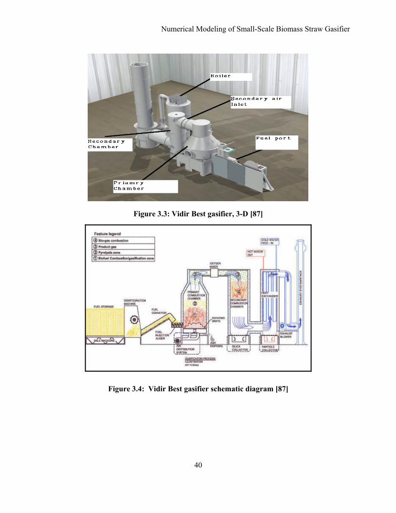
Numerical Modeling of Small-Scale Biomass Straw Gasifier
40
Figure 3.3: Vidir Best gasifier, 3-D [87]
Figure 3.4: Vidir Best gasifier schematic diagram [87]

Numerical Modeling of Small-Scale Biomass Straw Gasifier
41
Figure 3.5: Secondary chamber characterized by high temperature
3.5 Modeling gasification
Biomass gasification and pyrolysis are thermally degraded processes in the absence of air or
oxygen for producing solid charcoal, or liquid fuels like bio-oil and gaseous products for syngas
production [88]. CFD numerical models can be used to describe these processes because they
have become an important analysis and design tool to achieve the flow and temperature pattern,
the products’ concentration contour, and yields [20].
The understanding of the interaction between chemical and physical mechanisms during
gasification/combustion is of fundamental importance for the optimal design of a biomass
gasifier [89], to address control problems, scale up, and resolve issues. In view of the
considerable interest in the gasification process worldwide, it is necessary to model and predict
the performance of the gasifier to improve designs and solve operational problems. Modeling of
biomass gasification implies representing chemical and physical phenomena constituting fuel
drying, pyrolysis, gasification, combustion and char reduction in mathematical form.

Numerical Modeling of Small-Scale Biomass Straw Gasifier
42
There are several modeling studies on packed-bed biomass combustion. Lists of some studies are
tabulated in Table 3.2. Zhou et al. [54] numerically modelled the combustion of straw in a
bench-top stationary fixed bed with focus on NO formation and reduction. Higman et al. [72]
employed a two-dimensional model for straw combustion in a moving bed where the bed is
assumed to be at steady state, and the time elapsed since ignition is related to a horizontal
position on the grate by a simple linear function. The model was validated based on fixed-bed
experiments. Kaer [30, 33] carried out numerical modeling of a 33 MW straw-fired grate boiler
incorporating a stand-alone bed model and a commercial CFD code for gas-space computation.
He concluded that poor mixing in the furnace is a key issue leading to high emission levels and
relatively high amounts of unburnt carbon in the fly ash. The stand-alone bed model is based on
a one-dimensional “walking-column” approach and included the energy equations for both the
fuel and the gas accounting for heat transfer between the two phases.
The above models have the disadvantage of not taking the particle mixing effect into account
when applied to a moving-grate. Yang et al. [90] have indicated that solid-fuel mixing caused by
the grate movement can significantly enhance the reaction rates of biomass fuel in a packed-bed,
and hence can change the combustion characteristics of the furnace. The latter work overcame
the shortcomings of the previous modeling works on straw combustion by introducing a particle
mixing coefficient in the model. This method helped to further understand the operating
characteristics of large-scale, straw-burning plants.
Many researchers have developed models for biomass gasification [3, 18 and 78].
Zainal et al. [91] used the equilibrium model to predict the composition of producer gas.
Fletcher et al. [27] developed a detailed CFD model to simulate the flow and reaction in an
entrained-flow biomass gasifier. The model is based on the Computational Fluid DynamiX
(CFX) package and describes the phenomena of turbulent fluid flow, heat transfer, species
transport, devolatilization, particle combustion, and gas phase chemical reactions. Biomass
particulate is modelled via a Lagrangian approach because it entered the gasifier, released its
volatiles and finally underwent gasification. Transport equations were solved for the
concentration of CH4, H2, CO, CO2, H2O and O2 and heterogeneous reactions between fixed
carbon and O2, CO2 and H2O were modelled. The model provided detailed information on the

Numerical Modeling of Small-Scale Biomass Straw Gasifier
43
gas composition and temperature at the outlet and allowed different operating scenarios to be
examined in an efficient manner. The initial calculations suggested that simulations to examine
the effect of gasifier height and the steam flux in the upper inlets could be beneficial in process
optimization. The simulation of sawdust gasification in one case gave an exit composition on a
dry basis of 10% CO, 12% CO2, 20% H2 and 1.2% CH4; compared with 16% CO, 14% CO2,
10% H2, and 1% CH4 measured in the experiments, the hydrogen generation was too high. The
effects of initial moisture content in the wood and the temperature in the gasification zone on the
calorific value were investigated.
Mathieu and Dubuisson [82] developed a model based on minimization of Gibbs free energy
which was performed in the 1-D ASPEN PLUS process simulator. The effects of the oxygen
factor, the air temperature, operating pressure and the injection of steam were studied. Di
Blasi [7] developed a one-dimensional, unsteady-state model for biomass gasification in a
stratified concurrent downdraft reactor. Heat and mass transfer across the bed were coupled with
moisture evaporation, biomass pyrolysis, char combustion, and gasification, gas-phase
combustion and thermal cracking of tars. The model was used to simulate the structure of the
reaction fronts and the gasification behaviour of a laboratory-scale plant as the reactor
throughput and the air-to-wood or char weight ratio were varied.
Giltrap et al. [92] developed a model for the reduction zone of a downdraft biomass gasifier to
predict the composition of producer gas under steady-state operation. Factors affecting the gas
composition were the fraction of pyrolysed gas in the initial gas entering the reduction zone of
the biomass gasifier, air-to-fuel ratio, moisture content of biomass, bed temperature, and
reactivity of char. Molar balance, energy balance, pressure gradient equation, and Arrhenius type
of temperature dependence kinetic equation formed the set of first order differential equations,
which were solved by finite difference method. The accuracy of the model was limited by the
availability of data on the initial conditions at the top of the reduction zone. Moreover it was
assumed that char reactivity factor (CRF), which represented the reactivity of char and the key
variable in simulation, was constant throughout the reduction zone. Kaer et al. [93] developed a
model incorporating Milligan’s [84] flaming pyrolysis sub-model along with the gasification
zone sub-model. The model did not include the effect of packed char particles in a reduction

Numerical Modeling of Small-Scale Biomass Straw Gasifier
44
zone because it was limited by considering only a single particle. Babu and Sheth [56] modified
Giltrap’s model by incorporating the variation of CRF along the reduction zone of the downdraft
biomass gasifier. The model was simulated with the finite difference method to predict the
temperature and composition profiles in the reduction zone. A finite difference technique was
successfully applied to solve such type of partial differential equations in other studies [65, 82].
The CRF value is increased linearly and exponentially along the reduction bed length in the
model. The model predictions were compared with the experimental data reported by
Kaer et al. [93]. Babu and Sheth [50] studied the effects of pyrolysis fraction and bed
temperature on gas compositions.
The crucial combustion parameter, primary air flow rate, has been widely studied by researchers
such as Dixon et al. [11], Roos et al. [36], Moilanen, A. & Saviharju [49], Gil et al. [88],
Yang et al. [90]. Luo et al. [99] developed a two-dimensional steady model for straw combustion
in a cross-current moving bed and verified the model with experimental data for the effects of the
inlet air flow rate and air temperature on the combustion process. Their work was extended by
Zhou et al. [54] who developed a one-dimensional transient model of fixed-bed straw
combustion and validated the results with experimental measurements of temperature, gas
emissions, and ignition front propagation rate and flame temperature. Kaer [79] investigated a
straw-fired grate boiler using the computation fluid dynamics (CFD), in which the model
predictions were compared with measurements obtained from a full-scale boiler plant at
Masnedø (Denmark). Rapagnà et al. [94] investigated the physical and chemical transformation
of biomass chars (pine and switch grass) during combustion. A major problem associated with
the utilization of straw is the low ash melting temperature, producing cakes of sintered ash.
Olivares et al. [73] carried out the characterization of ashes from wood and straw.
Gerun et al. [95] developed a 2-D axisymmetric CFD model for the oxidation zone in a two-
stage, downdraft gasifier. The oxidation zone is crucial for tar cracking. The simulations fit
satisfactorily to the experimental data regarding temperature pattern and tar concentration. The
heat of reaction was released mainly close to the injector. It induced a hot zone in this area. The
gas path strongly depended on the initial departure point. The strong recirculation zone was

Numerical Modeling of Small-Scale Biomass Straw Gasifier
45
located above the air injection in the centre of the reactor. It played a major role in air-gas
mixing and thus enhanced the quality of the gasification.
Baxter [57] conducted a study on eleven biomass fuels representing a broad class of
commercially available fuels: straws and grasses, pits, shells, hulls and other lignocellulosic
biomass, woods and waste fuels of commercial interest. A systematic and reasonably detailed
analysis of fuel property, operating condition, and boiler design issues that dictate ash deposit
formation and property development was provided.
Table 3.2: Summary of CFD modeling attempts
Application Code Dim
Turb. Model
Extra Model Agreement with Exp.
Authors
Two-stage downdraft
gasifier
Fluent
2-D
RNG k-ε DOM Satisfactory Gerun, L. (2008)
Cone calorimeter
reactor
Code
1-D
N/A Porous N/A Giltrap, G.L. (2003)
Entrained flow gasifier
CFX
2-D
Std k-ε Langragian, DTRM
N/A Ma, et al. (2007)
Downdraft gasifier
Code
1-D
N/A Porous N/A Sharma, A.K.(2007)
Horizontal entrained flow
reactor
Fluent
1-D
N/A Langragian Reasonable Zhou, S.N. (2006)
Moving packed bed
Fluent
2-D
Std k-ε DOM N/A Kaer, S.K.
(2004)
Entrained flow gasifier
CFX4
2-D
Std k-ε RSM, Langragian
Acceptable Feltcher, D.F. (2000)
Herbaceous fuels contain silicon and potassium as principal ash forming constituents. They are
also high in chlorine and exhibit severe ash deposition problems due to the reaction of alkali with
Numerical Modeling of Small-Scale Biomass Straw Gasifier
46
silica to form alkali silicates that melt or soften at temperatures as low as 700oC and due to the
reaction of alkali with sulphur to form alkali sulphates on heat transfer surfaces. All biologically
active alkali, potassium in particular is traced to be the principal cause of most deposits. There
also exists the non-biological form of the alkali in soils and it exhibits much less reactivity. As
potassium is the cause of deposits in biomass, sodium does the same with coal.
Ma et al. [96] performed CFD application in a 1 MW industrial wood test furnace coupled with
the potassium release and NOx formation model. The potassium release during biomass
combustion is still a subject of current investigation. Ma et al. assumed that the biomass
potassium release during devolatilization rapidly forms KOH. Both the HCN and the NH3 route
have been considered for the NOx formation. The particle tracks and temperature distribution are
also studied in this work. Good agreement between the predicted and the measured furnace
temperature and concentrations of CO2 and NOx were achieved.
3.6 Ash deposition mechanism
Understanding ash deposition is critical to the proper functioning of a gasifier to ensure
convection section tubes stay unfouled. Biomass fuels contain considerable quantities of ash,
forming elements in addition to their main organic constituents C, H, O, and N [90]. The most
important of these elements are Si, Ca, Mg, K, Na, S, Cl as well as heavy metals such as Zn and
Pb [47, 89]. A typical composition of the most commonly used solid biomass fuels data reveals
extreme variations in ash content and ash composition between and within the different types of
biomass fuels. Wood has much lower ash content, for example, than bark, waste wood and
herbaceous fuels [95].
There are generally two sources for inorganic ash forming matter in biomass fuels [97]. Ash
forming elements originate from the plant itself, because they are part of the structure of the
fibers (e.g.: Si, Ca) or are macro or micro plant nutrients (e.g.: K, P, S, Zn) [98]. Alternatively,
inorganic matter in biomass fuels can also come from contamination with soil, sand or
stones [88]. Coatings, paints, glass pieces and metal parts are major sources of contamination in
waste wood [88].

Numerical Modeling of Small-Scale Biomass Straw Gasifier
47
Upon entering the combustion unit, the fuel is first dried, followed by devolatilization of the
volatile organic matter. Subsequently, the remaining fixed carbon is oxidized during
heterogeneous gas-solid reactions, which is called char combustion [55]. During these steps the
ash forming elements behave in two different ways according to their volatility [99]. Non-
volatile compounds such as Si, Ca and Mg are engaged in ash fusion as well as coagulation
processes [94]. Once the organic matter has been oxidized, these elements remain as coarse ash
structures. Easily volatile species such as K, Na, S, Cl, Zn and Pb generally behave
differently [97]. A considerable proportion of these elements are released to the gas phase due to
the high temperatures occurring during combustion [82]. There they undergo homogeneous gas
phase reactions and later on, due to super saturation in the gas phase, these ash forming vapours
start to nucleate, leading to the formation of submicron aerosol particles or condensation on
surfaces of existing particles [47]. The submicron particles are so-called aerosols and form one
important fraction of the fly ashes.
The processes that govern ash deposition can be divided into five categories: inertial impaction,
eddy impaction, thermophoresis, condensation and chemical reaction [55]. The net deposition
rate can be represented as the sum of these deposition mechanisms [99].
Inertial impaction is believed to be the dominant deposition mechanisms on chamber walls or at
any location where entrained ash particles are required to turn sharp corners at high velocity [60].
Inertial impaction occurs when a particle has sufficient momentum to impact an obstruction by
penetrating the flow field surrounding the obstruction [56]. Of the particles that do reach the wall
some fraction will tend to stick to the tube and become deposited there. The tendency of particles
to stick to the wall is thought to depend on the properties of the particle at the moment of impact
as well as those of the impacted surface, especially the previously accumulated ash layer [102].
While the physics that lead to particle impaction are fairly well understood, predicting what
fraction of impacting particles will stick is much more difficult [78]. As shown in Equation 14,
inertial deposition can be thought of as the product of impaction efficiency, η, and capture
efficiency, G, which together forms collection efficiency (ζ) [75]:

Numerical Modeling of Small-Scale Biomass Straw Gasifier
48
GAm
m
CrossAsh
Deposit .ηξ ==&
& (14)
3.6.1 Deposition mechanisms
3.6.1..1.1 Eddy impaction
Eddy impaction occurs when fine ash particles located near a solid surface are a blown by
turbulent eddies onto the surface where they become deposited [98]. In part, because of the
complexities of describing near-wall turbulent eddies, this mechanism is not well
understood [60].
3.6.1..1.2 Thermophoresis
Steep thermal gradients surrounding a particle can give rise to thermophoretic forces [85].
Thermophoresis, which is significant only for fine particles, typically transports particles towards
regions of lower temperature, which, in the case of a cooled section of a chamber, drives
particles toward the wall and can lead to deposition [103]. Ash deposited by thermophoresis is
generally more evenly distributed around a wall whereas inertial impaction occurs only on the
chamber’s upstream side [102]. Thermophoretic deposition also decreases as the insulating layer
of ash accumulates and the temperature difference between the gas and the deposit surface
temperature decreases [85].
3.6.1..1.3 Condensation
Condensation occurs when mass from the gas phase collects on a cool surface [38]. Relatively
low temperatures near a cooled chamber can cause certain gas-phase constituents to condense
and accumulate [47]. In addition to temperature, condensation also depends on the
concentrations of these various constituents in the gas phase [82]. Condensation is typically of
greater concern in biomass applications or wherever a large amount of inorganic material
particularly alkali salts, is present in the fuel [74]. Condensation may be the mechanism that
allows the silica to slag in the Vidir downcomer.

Numerical Modeling of Small-Scale Biomass Straw Gasifier
49
3.6.1..1.4 Chemical reaction
Chemical reactions between the solid and gas phases can also change the net rate of mass
deposition [46]. These reactions may also affect the properties of the ash deposit by changing the
temperatures at which sintering and melting occur, which can in turn affect the number of
particles captured during inertial impaction processes [101].
3.6.1..1.5 Other mechanisms
Several other mechanisms exist which may play a role in deposit formation. These other
mechanisms include electrostatic forces, photophoresis, and Brownian motion. Current
understanding however suggests that these mechanisms are not significant in the formation of
deposits [47].

Numerical Modeling of Small-Scale Biomass Straw Gasifier
50
Chapter 4. Numerical simulation methodology
Using the CFD commercial software, FLUENT 6.2®, a model of the gasifier was developed to
understand the combustion/gasification mechanism of biomass fuel, particularly straw, and
applied to the Vidir gasifier. A CFD model mainly consists of three main parts. The first part is
the physical models which are a set of conservation equations of mass, momentum, energy, state
equation, turbulent equations, chemical reaction and source term equations. The second part is a
series of solution approaches for solving these physical models and the third part is the pre-
processor of discretization of computational domain and the postprocessor of visualization of
numerical results.
As a CFD code, FLUENT® solves the fundamental conservation equations for microscopic
regions [105]. It solves the Navier-Stokes equations using a finite volume method on a grid,
which is generated directly integrated in FLUENT® 6.2 [93]. Boundary conditions and selecting
the right sub-model have critical importance in the model of a system. Discussions on the
available options to address major problems in achieving heat transfer, turbulence and species
evaluation leading to ways to set up an adequate gasifier model are emphasized. The sub-models
and solution methods available in FLUENT®, and those chosen in the model are also discussed
in detail in this chapter.
4.1 Basic governing equations
For a homogenous Newtonian fluid flow, the mathematical modeling was based on a set of
coupled conservation equations of mass, momentum, energy, and chemical species transport and
reactions, and the state equations of the fluid system [79]. Furthermore, since most practical
flows are turbulent, these conservation equations should be treated into the time-averaged or
spatial filtered forms, which needed to be closed by using additional turbulent models [57].
4.1.1 Conservation Equations
A numerical study was performed for obtaining the flow field characteristics of the Vidir
Gasifier. It involved solving the following equations [18]:

Numerical Modeling of Small-Scale Biomass Straw Gasifier
51
( ) iii
Suxt
=ρ∂∂
+∂ρ∂
(15)
where Si mass source in the system.
For a multi-component system, the mass balance can be expressed as [96]:
( ) ( )iiii
ii
iii SRJXX
mutm
′′′′′ ++
∂∂
−=∂
∂+
∂∂
,ρρ (16)
where mi’ local mass fraction of each species in the system
J i’,i diffusion flux of species i’, which arises due to concentration gradients
Ri’ mass rate of creation or depletion by chemical reaction
Si’ mass rate of any other sources
For laminar flows of dilute gas system, the diffusion flux meets the Fick’s law as [48]:
i
imiii x
mDJ∂∂
−= ′′′ ,, ρ (17)
where D i’, m diffusion coefficient for species i’ in the mixture
The conservation equations of momentum can be described as Navier-Stokes equations as [84]:
( ) ( )mi
j
ij
ij
jii SxX
pX
uutu
+∂
∂+
∂∂
−=∂
∂+
∂∂ τρρ (18)
where p static pressure
τij stress tensor
Smi momentum source in i direction
The stress tensor τij is given by [105]:
iji
i
i
j
j
iij x
uxu
xu
δμμτ∂∂
−⎟⎟⎠
⎞⎜⎜⎝
⎛
∂
∂+
∂∂
=32 (19)
where μ molecular viscosity.

Numerical Modeling of Small-Scale Biomass Straw Gasifier
52
The conservation equation of energy can be written as [95]
( ) ( ) hk
iikjj
jiiiii
i
Sxu
Jhxx
TKxpu
tphu
Xth
+∂∂
+∂∂
−⎟⎟⎠
⎞⎜⎜⎝
⎛∂∂
∂∂
+∂∂
=∂∂
+∂
∂′′
′
τρρ
where 'jj hmh = , ∫=
T
Tjpj
ref
dTCh ., (20)
The energy source due to chemical reactions can be expressed as [91]
jj
jpTT
j
of
reactionh RdTCMh
S ref
ret ′′
′′
∑ ∫+= ,, (21)
and the energy source due to radiation was calculated in radiation models.
4.1.2 General transport equation
For a general variable Φ of the fluid, such as mass or species, momentum, energy, the above
conservation equations can be summarized into a general transport equation of Φ as [48]
( ) ( )φφ
φρφρφ SxXXt ijj
j +⎥⎦
⎤⎢⎣
⎡∂∂
Γ∂∂
=∂
∂+
∂∂
(22)
where ΓΦ transport coefficient of the general variable Φ
For a perfect gas system, the state equations can be written as [79]:
i
iNi M
mRTp 1== ρ (23)
where mi and Mi are the mass fraction and the molecular weight of the ith species, respectively.
4.2 Turbulence models
The above basic governing equations for a homogenous Newtonian fluid flow form a closed set
of partial differential equations (PDE) [48]. This situation is only suitable to numerically solve a
laminar flow. For turbulence, it can be characterized as a three dimensional, time-dependent,

Numerical Modeling of Small-Scale Biomass Straw Gasifier
53
chaotic, random and dissipative flow [79]. In a turbulent flow, there exists an energy cascade
corresponding to a wide range of length scales from largest eddies (anisotropic integral length
scales) to smallest eddies (isotropic Kolmogorov length scales) [35]. Therefore, the direct
numerical simulation (DNS) of a turbulent flow with a high Reynolds number in a complicated
modern furnace or boiler is practically impossible even with today’s computer capacity [79].
For most engineering applications, the time-averaged or spatial filtered properties of the flow are
of interest, thus the time-averaged transport equations, such as the Reynolds averaged Navier-
Stokes (RANS) equations, were established [97]. However, time-averaged equations are not in a
closed form and thus additional closure methods corresponding to different turbulence models
had to be developed [91].
The most often used method is one that is arranged in order of the number of differential
equations solved for turbulence: zero-, one-, two- and stress equation models as presented by
Bentzen [55]. According to Bentzen
• Zero equation models are based mostly on the eddy viscosity concept and give the shear
stress. They need a field of mixing length, which can be difficult to obtain in 3-D
complex flows.
• One equation models solve the equation for turbulent kinetic energy. They need a field of
a turbulent length scale for calculating dissipation and effective viscosity. In rapid
transient flows, one equation models with the length scale set proportional to the grid size
may give more representative turbulence field than other models.
• Two equation models are most widely used in present day engineering calculations. The
length scale used here was found from an algebraic relation with the solution of a second
equation. The most popular two equation model is the k-ε model, presented in the next
section. There are also stress equation models that calculate the Reynolds stresses either
through an algebraic relation with k, as the algebraic stress models, or by replacing the
equation for k with equations for the Reynolds stresses.
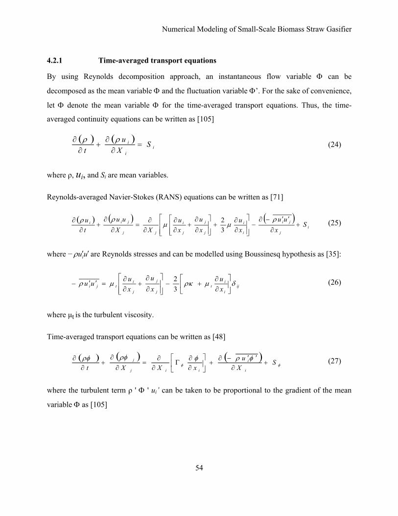
Numerical Modeling of Small-Scale Biomass Straw Gasifier
54
4.2.1 Time-averaged transport equations
By using Reynolds decomposition approach, an instantaneous flow variable Φ can be
decomposed as the mean variable Φ and the fluctuation variable Φ’. For the sake of convenience,
let Φ denote the mean variable Φ for the time-averaged transport equations. Thus, the time-
averaged continuity equations can be written as [105]
( ) ( )i
i
i SX
ut
=∂
∂+
∂∂ ρρ (24)
where ρ, ui, and Si are mean variables.
Reynolds-averaged Navier-Stokes (RANS) equations can be written as [71]
( ) ( ) ( )i
j
ji
i
i
j
j
j
i
jj
jii Sx
uuxu
xu
xu
XXuu
tu
+∂
′′−∂−
⎥⎥⎦
⎤
⎢⎢⎣
⎡
∂∂
+⎥⎥⎦
⎤
⎢⎢⎣
⎡
∂
∂+
∂∂
∂∂
=∂
∂+
∂∂ ρ
μμρρ
32 (25)
where − uui ′′ρ are Reynolds stresses and can be modelled using Boussinesq hypothesis as [35]:
iji
it
j
j
j
itji x
uxu
xuuu δμρκμρ ⎥
⎦
⎤⎢⎣
⎡∂∂
+−⎥⎥⎦
⎤
⎢⎢⎣
⎡
∂
∂+
∂∂
=′′−32 (26)
where μt is the turbulent viscosity.
Time-averaged transport equations can be written as [48]
( ) ( ) ( )φφ
φρφρφρφ SX
uxXXt i
i
iij
j +∂
′′−∂+⎥
⎦
⎤⎢⎣
⎡∂∂
Γ∂∂
=∂
∂+
∂∂ (27)
where the turbulent term ρ ' Φ ' ui’ can be taken to be proportional to the gradient of the mean
variable Φ as [105]

Numerical Modeling of Small-Scale Biomass Straw Gasifier
55
( ) ⎥⎦
⎤⎢⎣
⎡∂∂
Γ∂∂
=′′−ii
i xXu φφρ φ
(28)
where ΓΦ is the turbulent transport coefficient of the mean variable Φ .
The time-averaged transport equations, including the turbulent transport coefficient, such as
turbulent viscosity μ t in RANS, needs to be modelled [105].
a. The Standard k-ε Model
Launder and Spalding [81], developed the standard k-ε mode to close the time-averaged systemic
PDEs. The k-ε model equations are derived from the RANS equations, and the various model
constants, and rely on phenomenological considerations and empiricism. By using dimensional
analysis, the turbulent viscosity μ t can be assumed as [48]
VLCt ρμ = (29)
where C dimensionless constant
V turbulent velocity scale (m/s)
L turbulent length scale (m)
According to dimensional analysis, the turbulent velocity scale, V, and the length scale, L, can be
defined by using two quantities of turbulent kinetic energy κ and its rate of dissipation ε as [79]:
εκκ
23
21
== LandV (30)
Thus the turbulent viscosity can be evaluated by k and ε as [65]:
εκμρμ
2
Ct = (31)
where C μ is a dimensionless constant.
In the standard k-ε model, the k and ε can be obtained from the following transport equations
as [91]

Numerical Modeling of Small-Scale Biomass Straw Gasifier
56
( ) ( )ρεκ
δμ
μκρρκ
κκ
−+−⎥⎦
⎤⎢⎣
⎡
∂∂
+⎥⎦
⎤⎢⎣
⎡+
∂∂
=∂
∂+
∂∂
bi
t
ii
i GGxXX
ut
(32)
( ) ( )κερ
κεε
δμ
μερρε
εεκεε
2
231 ))1(( CGCGCxXX
ut b
i
t
ii
i −−+−⎥⎥⎦
⎤
⎢⎢⎣
⎡
∂∂
+⎥⎦
⎤⎢⎣
⎡+
∂∂
=∂
∂+
∂∂ (33)
where Gk is the generation of k due to the turbulent stress as [71]
( )i
jij
i
jji x
uXu
uuG∂
∂=
∂
∂′′−= τρκ (34)
It can be evaluated by Boussinesq hypothesis as [93]
2SG tμκ = (35)
where S is the modulus of the mean strain rate and Sij expressed as [71]:
⎥⎥⎦
⎤
⎢⎢⎣
⎡
∂
∂+
∂∂
==i
j
j
iijijij x
uxu
SandSSS212 (36)
Gb is the generation of k due to the buoyancy as [105]
it
tib x
TG∂∂
=Prμ
β (37)
where Prt is the turbulent Prandtl number for temperature or enthalpy and β is the coefficient of
thermal expansion as [35]
pix ⎥⎦
⎤⎢⎣
⎡∂∂
−=ρ
ρβ 1 (38)
This method is popular and widely used in practical engineering turbulent flow problems [61].
For this reason the standard κ- ε model was used for the simulations in this thesis. The standard
k-ε model constants C1ε, C2ε, Cμ, σk, σε, values used are C1ε = 1.44, C2ε = 1.92, Cμ = 0.09,

Numerical Modeling of Small-Scale Biomass Straw Gasifier
57
σk = 1.0, σ ε = 1.3 [81]. This semi-empirical model is robust, economical, and reasonably
accurate.
b. The RNG k-ε model
The RNG model [44] was developed in response to the empirical nature of the standard k-ε
model. Rather than being based on observed fluid behaviour, it was derived using statistical
methods used in the field of renormalization group (RNG) theory [44]. The transport equations
for turbulent kinetic energy k and its dissipation rate ε in RNG k-ε model have the same forms as
in the standard k-ε model except of the additional quantities of the inverse effective Prandtl
numbers α k and α ε, and the R term in the ε equation [48].
( ) ( )ρεκ
δμ
μακρρκ
κκ
κ −++⎥⎦
⎤⎢⎣
⎡
∂∂
⎥⎦
⎤⎢⎣
⎡∂∂
=∂
∂+
∂∂
bi
teff
ii
i GGxXX
ut
)( (39)
( ) ( ) RCGCGCxXX
ut b
i
teff
ii
i −−−+−⎥⎥⎦
⎤
⎢⎢⎣
⎡
∂∂
⎥⎦
⎤⎢⎣
⎡∂∂
=∂
∂+
∂∂
κερ
κεε
δμμαερρε
εεκεε
ε
2
231 ))1(()( (40)
κε
βηηηρημ 2
30
3
1
1
+
⎟⎟⎠
⎞⎜⎜⎝
⎛−
=C
R (41)
where η0 = 4.38
β = 0.012
εη κS
= (42)
The effective viscosity can be solved by the following equations as [57]
μμ
ν
νν
νβεμκρ
ν
eff
i wheredC
d
=
+−=
⎥⎥⎦
⎤
⎢⎢⎣
⎡
)
))
)
172.1
3
2
(43)

Numerical Modeling of Small-Scale Biomass Straw Gasifier
58
In the RNG k-ε model, the effects of swirl can be accounted for by modifying the turbulent
viscosity as [27]
⎟⎠⎞
⎜⎝⎛ Ω=
εκαμμ ,,sefft f (44)
where α s swirl constant (0.05 at mildly swirling flows).
Ω characteristic swirl number.
The RNG k-ε model constants C1ε and C2ε have the following values:
C1ε = 1.42, C2ε = 1.68
In both k-ε model transport equations 33, 40, the model constant C3ε for buoyancy term can be
calculated as [48]
ενμε tanh3 =C (45)
where, v is the velocity component parallel to the gravitational vector and u is the velocity
component perpendicular to the gravitational vector.
c. Standard k–ω model
The last turbulence model that will be discussed is the κ–ω model. This model is based on the
Wilcox k–ω model [48]. It incorporates modifications for low-Reynolds number effects,
compressibility and shear flow spreading. The Wilcox model predicts free shear flow spreading
rates that closely agree with measurements for far wakes, mixing layers and different types of
jets. Therefore this model applies to both wall-bounded flows and free shear flows.
The k-ω model is a two-equation, semi-empirical turbulence model [48]. The transport equation
for the kinetic energy is comparable with the previous k–ε models. The equation for the
dissipation on the other hand, is different. Instead of the dissipation per unit of mass, the specific
dissipation rate ω is used. This quantity can be seen as the ratio of ε to κ [40].

Numerical Modeling of Small-Scale Biomass Straw Gasifier
59
4.2.2 The Reynolds stress model
In this model, using the Boussinesq relation, the Reynolds stresses (ρ u' i u' j) are linked to the
mean flow velocities, such as in k-ε models [27]. However, these kind of models of first moment
closure approach are quite limited in predicting the flows with complex strain fields or
significant body forces [57]. This drawback advocated Launder et al. [40] to have developed a
more complex second-moment closure approach, so called Reynolds stress model (RSM), in
which the Reynolds stresses are modelled using both the mean flow velocities and the first-
moment terms.
4.3 Near-wall treatments for turbulent flows
Turbulence models are largely valid for turbulent core flows, i.e., flows in the regions somewhat
far from walls [79]. When the flow to be calculated involves walls, turbulent flows in the regions
close to the walls are affected by the presence of the walls. First, the mean velocity field is
affected through the no-slip condition that has to be satisfied at the wall. Turbulence is also
changed by the presence of the wall. Close to the wall, turbulence is damped due to the presence
of walls. Toward the outer part of the near-wall region, turbulence is rapidly augmented by the
production of turbulent kinetic energy due to Reynolds stresses and the large gradient of the
mean velocity [50].
Experiments have shown that the near-wall region can be largely subdivided into three
layers [35]. In the innermost layer called the viscous sub-layer, the flow is almost laminar-like,
and the viscosity plays a dominant role in momentum and heat transfer [35]. In the outer layer,
called the fully-turbulent layer, turbulence plays a major role [79]. Finally, there is an interim
region between the viscous sub-layer and the fully-turbulent layer called the buffer layer where
the effects of viscosity and turbulence are equally important [61].
In the near-wall region, the velocity has a universal distribution [56]. Numerous measurements
of this distribution exist. According to these measurements, the viscous sub-layer and the fully
turbulent region can be represented as functions between the dimensionless wall distance y+ and
the dimensionless velocity u+ as [56]

Numerical Modeling of Small-Scale Biomass Straw Gasifier
60
For viscous sublayer: u+ = y+ 0 < y+ < 5
For full-turbulent region: u+ = 1/κ ln y+ + C+ 30 < y+
where τu
uu =+ , μ
ρ τ yuy =+ , ρ
τ ωτ =u (46)
and κ Karman constant, 0.42
C+ empirical constant, 5.0
τω Wall shear stress
Y normal distance to the wall
Figure 4.1: Universal log law [71]
There are two approaches for treating of the near-wall region [54]. The first one does not solve
the viscous affected region that is the buffer layer and viscous sub-layer [33]. Instead the first
method uses semi-empirical formulas to bridge the region between the wall and the fully
turbulent flow [71]. These formulas are called wall functions [71]. The second approach
modifies the turbulence models to enable the viscosity affected region to be resolved all the way

Numerical Modeling of Small-Scale Biomass Straw Gasifier
61
to the wall [95]. In this case the mesh must be fine enough. This method is called near-wall
modeling [50].
Figure 4.2: Near wall grids [71]
There are two wall function approaches offered in Fluent® [109]:
a. Standard wall functions: (standard in industrial applications and the default in Fluent).
The logarithmic law for mean velocity farther away from walls (turbulent region) and
linear closer is applied to solve for the momentum [61]. The energy and species transport
equations are solved using a linear law for a thermal conduction sublayer and a
logarithmic law for the turbulent region, whereas to solve for turbulence in both k-ε
models and in RSM, the k equation is solved in the whole domain including the wall-
adjacent cells [56].
b. Non-equilibrium wall functions: This approach uses the log-law for mean velocity
sensitized to pressure-gradient effects and a two-layer (viscous and fully turbulent layers)
base that allows for computing of turbulence kinetic energy in wall-adjacent cells [71].
Standard wall function has a low computational burden with limitations only to
applications where there is a pervasive low-Reynolds-number or near-wall effects (e.g.
flow through a small hole, or highly laminar flow), massive transpiration through the wall
(blowing/suction), large pressure gradients, strong body forces (e.g. flow near a rotating
body) or high three dimensionality near the walls (e.g. strongly skewed flows) [54]. Since

Numerical Modeling of Small-Scale Biomass Straw Gasifier
62
none of these characteristics were exhibited in the gasifier, which is the subject of
investigation, the standard wall functions was used.
4.4 Radiation modeling
The radiative transfer equation (RTE) for an absorbing, emitting, and scattering medium at
position r in the direction s can be written as follows [53]:
Ω ′′Φ′+=++ ∫ dsrsrITansrIads
srdI ss ),(),(
4),()(),( 4
0
42
π
πσ
πσσ (46)
In Fluent, there are four common radiation models and these are [109]:
• P-1 Radiation Model
• Rosseland Model
• Discrete Ordinates Model (DOM)
• Discrete Transfer Radiation Model (DTRM)
4.4.1 P-1 model
P-1 model is the simplest formulation of the more general P-N radiation model, which is based
on the expansion of the radiation intensity I into an orthogonal series of spherical
harmonics [98]. The method of spherical harmonics provides a means to obtain an approximate
solution of arbitrary high order (i.e. accuracy), by transforming the radiative transfer equation
into a set of simultaneous partial differential equations [53]. Using only four terms in the series
solution of the respective differential equation, the following relation is obtained for the radiation
flux [53]:
Gqs
r ∇+
−=)(3
1σα
(47)
where G is the incident radiation. The problem is then much simplified since it is only necessary
to find a solution for G rather than determine the direction dependent intensity [53]. Then the
following expression for qr can be directly substituted into the energy equation to account for
heat sources (or sinks) due to radiation as follows:

Numerical Modeling of Small-Scale Biomass Straw Gasifier
63
44 TaaGq r σ−=∇− (48)
4.4.2 Rosseland model
The Rosseland radiation model can be derived from the P-1 radiation model with some
approximations. The radiative heat flux vector in a gray medium is approximated by [53]:
Gq r ∇Γ−= (49)
The Rosseland radiation model differs from the P-1 model in that the Rosseland model assumes
the intensity is equal to the black-body intensity at the gas temperature. Thus,
424 TnG σ= (50)
while the P-1 model actually calculates the transport equation for G. Substituting this value for G
into equation (49) yields:
TTnq r ∇Γ−= 3216σ (51)
This model is also called “diffusion approximation” model, since the radiation problem reduces
to a simple conduction problem with strongly temperature dependent conductivity [96]. It is
important to keep in mind that the diffusion approximation is not valid near a boundary [54].
4.4.3 Discrete transfer radiation model
The main assumption of the Discrete Transfer Radiation Model (DTRM) is that the radiation
leaving the surface element in a certain range of solid angles can be approximated by a single
ray [53]. The equation for the change of radiant intensity, dI, along a path, ds, can be written
as [65]
πσ 4TaaI
dsdI
=+ (52)
Here, the refractive index is assumed to be unity. The DTRM integrates Equation 52 along a
series of rays emanating from boundary faces. If a is constant along the ray, then I (s) can be
estimated as [105]

Numerical Modeling of Small-Scale Biomass Straw Gasifier
64
aso
as eIeTsI −− +−= )1()(4
πσ
(53)
The “ray tracing” technique used in the DTRM can predict of radiative heat transfer between
surfaces without explicit view-factor calculations. The accuracy of the model is limited mainly
by the number of rays traced and the computational grid [55].
4.4.4 Discrete ordinates model
The Discrete Ordinates Model (DOM) solves the radiative transfer equation (RTE) for a finite
number of discrete solid angles, each associated with a vector direction s i (i = 1, 2,...n) fixed in
the global Cartesian system, and the integrals over these directions are replaced by numerical
quadratures [91]. The DOM considers the RTE in the direction si as a field equation, thus the
RTE is transformed into a transport equation for radiation intensity in the spatial
coordinates [79]:
( )( ) Ω ′′Φ′+=++•∇ ∫ dsrsrITansrIassrI ss ),(),(
4),()(,
4
0
42 rrrrrrrrr π
πσ
πσσ (54)
The standard form DOM suffers from a number of serious drawbacks, such as false scattering
and ray effects [95]. Perhaps the most serious drawback of the method is that it does not ensure
conservation of radiative energy. This is because the standard discrete ordinates method uses a
simple quadrature for angular discretization. Thus, it is a logical step in the evolution of the
method to move to a fully finite volume approach, in space and in direction. The finite volume
method uses an exact integration to evaluate solid angle integrals and the method is fully
conservative [56].
The optical thickness aL where L is an appropriate length scale is a good indicator of which
model to use. When aL >> l the P-1 and Rosseland models are suitable [53]. The P-1 model
should typically be used for optical thicknesses large than one [33]. The Rosseland model is
computationally cheaper and more efficient but should only be used for optical thicknesses larger
than three [65]. The DOM model works across the range of optical thicknesses, but is
substantially more computationally expensive than the Rosseland model [93]. The Rosseland

Numerical Modeling of Small-Scale Biomass Straw Gasifier
65
model does not take in to account for radiation exchange between gas and particulates.
Therefore, the DOM radiation model using the finite volume approach was considered for the
CFD model for the gasifier.
4.5 Species transport
The species equation accounts for the conservation of species. Multiple species equations can be
used to represent fluids in a mixture with different physical properties [104]. Solution of the
species equations can predict how different fluids mix, but not how they will separate [50].
Separation is the result of different body forces acting on the fluids, such as gravity acting on
fluids of different density [98]. To model the separation, separate momentum equations are
required for each of the fluids so that the body forces can act on the fluids independently [93].
Species transport is nevertheless a useful tool for predicting blending times or chemical
reaction [105]. For the species i’, the conservation equation is for the mass fraction of that
species, mi’, and has the following form [105]:
( ) ( ) iiiji
iii
i SRJX
mUXpm
t ′′′′′ ++∂∂
=∂∂
+∂∂
,ρρ (55)
In Equation 55, J i’,i is the i component of the diffusion flux of species i’ in the mixture. For
laminar flows, J i’,i is related to the diffusion coefficient for the species and local concentration
gradients. For turbulent flows, J i’,i also includes a turbulent diffusion term, which is a function
of the turbulent Schmidt number [71]. R i’ is the rate at which the species are either consumed or
produced in one or more reactions, and Si’ is a general source term for species. The general
source term can be used for non-reacting sources, such as the evaporated vapour from a heated
droplet, for example [48].
When two or more species are present, the sum of the mass fractions in each cell must add to 1.0.
For this reason, if there are n species involved in a simulation, only n-1 species equations need to
be solved. The mass fraction of the nth species can be computed from the required condition [65]:
1=∑ ′
n
iim (56)

Numerical Modeling of Small-Scale Biomass Straw Gasifier
66
A volumetric reaction with species transport can be handled in CFD using three different models
[98]:
1. laminar finite rate model: The effects of turbulent fluctuations are ignored, and reaction
rate is determined by Arrhenius expressions.
2. eddy-dissipation model: The reaction rates are assumed to be controlled by the
turbulence, so Arrhenius chemical kinetic calculations can be avoided.
3. eddy-dissipation concept model: A detailed Arrhenius chemical kinetics expression can
be incorporated into the turbulence flames.
It should be noted that detailed chemical kinetic calculations are computationally expensive in
the eddy-dissipation concept model. Eddy-dissipation model is robust and less demanding in
terms of inputs [56]. Therefore, eddy-dissipation is used for the gasifier simulations since it can
model reactions with relative ease without sacrificing accuracy.
4.6 Gaseous turbulent combustion models
The reaction rate of a gaseous reaction process is determined by mixing the reacting species, and
by the reaction kinetics, which is usually strongly depends on the reaction temperature in a
combustion chamber [98]. Actually, the combustion process, even only for simple fuel
combustion, concerns numerous intermediate reactions that are, in practice, impossible to
calculate in detail [79]. Therefore, some simplifications and assumptions have to be done to deal
with combustion reaction problems.
4.6.1 The generalized finite rate reaction modeling
The kth reaction taking place in a combustion system that contains N chemical species can be
described in general as [96]
)()(11
∑∑==
=n
pn
rk MM
κκκ
κκ νν (57)

Numerical Modeling of Small-Scale Biomass Straw Gasifier
67
where (Mk) denotes the concentration of species k in moles per unit volume, νrk are the
stoichiometric coefficients of the reactants, and νpk are the stoichiometric coefficients of the
products. When a species does not occur as a reactant or product, the corresponding coefficient is
zero [65].
The rate of disappearance of species k in an elementary reaction is governed by the law of mass
action, stating that it is proportional to the product of the concentrations of the reacting species,
where each species is raised to the power of the stoichiometric constant [88]. The law of mass
action can be verified experimentally and was first proposed by Obernberger and Joller [82]. The
reaction rate Rk is hence given by [56]
rj
n
jjMR νκκ )(
1∏=
= (58)
where k specific rate coefficient
Σνrk overall order of the reaction
νrj order of the reaction with respect to species k
The rate of change of the concentration of species k for a reaction with both forward and
reversible propagation becomes [102]
( )rj
rj n
j j
jbk
prn
j j
jfv
pr
wwM
dtd
ν
κ
ν
κκκ
ρθκν
ρθκνω ∏∏
== ⎥⎥⎦
⎤
⎢⎢⎣
⎡−
⎥⎥⎦
⎤
⎢⎢⎣
⎡==
11
& (59)
where: ( )rk
pk
pr ννν κ −=
Here Wk is the mean molecular weight
kfv and kbk forward and backward rate coefficients respectively
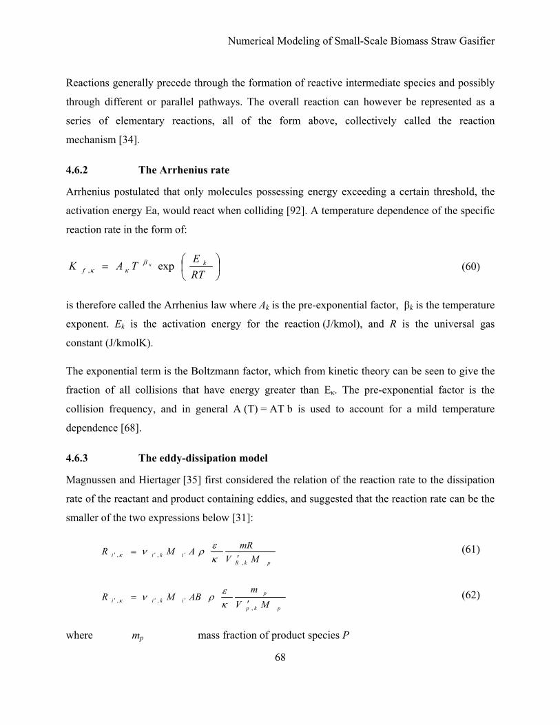
Numerical Modeling of Small-Scale Biomass Straw Gasifier
68
Reactions generally precede through the formation of reactive intermediate species and possibly
through different or parallel pathways. The overall reaction can however be represented as a
series of elementary reactions, all of the form above, collectively called the reaction
mechanism [34].
4.6.2 The Arrhenius rate
Arrhenius postulated that only molecules possessing energy exceeding a certain threshold, the
activation energy Ea, would react when colliding [92]. A temperature dependence of the specific
reaction rate in the form of:
⎟⎠⎞
⎜⎝⎛=
RTETAK k
f exp,κβ
κκ (60)
is therefore called the Arrhenius law where Ak is the pre-exponential factor, βk is the temperature
exponent. Ek is the activation energy for the reaction (J/kmol), and R is the universal gas
constant (J/kmolK).
The exponential term is the Boltzmann factor, which from kinetic theory can be seen to give the
fraction of all collisions that have energy greater than Eκ. The pre-exponential factor is the
collision frequency, and in general A (T) = AT b is used to account for a mild temperature
dependence [68].
4.6.3 The eddy-dissipation model
Magnussen and Hiertager [35] first considered the relation of the reaction rate to the dissipation
rate of the reactant and product containing eddies, and suggested that the reaction rate can be the
smaller of the two expressions below [31]:
pkRikii MV
mRAMR,
,, ′= ′′′ κ
ερνκ (61)
pkp
pikii MV
mABMR
,,, ′
= ′′′ κερνκ
(62)
where mp mass fraction of product species P

Numerical Modeling of Small-Scale Biomass Straw Gasifier
69
mR mass fraction of a particular reactant R
A and B empirical constants equal to 4.0 and 0.5, respectively
k/ε represents the time scale of the turbulent eddies.
The eddy dissipation model is based on the concept that chemical reaction is fast relative to the
transport processes in the flow [56]. When reactants mix at the molecular level, they
instantaneously form products. The model assumes that the reaction rate may be related directly
to the time required to mix reactants at the molecular level [82]. In turbulent flows, this mixing
time is dominated by the eddy properties, and therefore, the rate is proportional to a mixing time
defined by the turbulent kinetic energy, k, and dissipation, ε.
In the finite-rate/eddy-dissipation modeling, the smallest rate of those from the Arrhenius rate
expression or the eddy dissipation model is used as the reaction rate, which is used as the source
term in the species conservation and energy equations [78].
4.7 Dispersed or discrete phase model
The dispersed phase model uses the Navier-Stokes equations to describe a continuous fluid
phase, and a Lagrangian particle tracking method to describe a dispersed phase consisting of
particles, droplets, or bubbles [78]. Heat, mass, and momentum exchange is permitted between
the dispersed and fluid phases. Thus gas bubbles can rise in a liquid, sand particles can settle, and
water droplets can evaporate or boil, releasing steam to a background of warm gas [94]. The
model is widely used for coal and liquid fuel combustion, bubble columns, and gas spargers in
stirred tanks [47]. It is best when the dispersed phase does not exceed 10% by volume of the
mixture in any region [88].
4.7.1 Particle transport methods
There are two main families of methods to treat particle transport in fluid flows: Eulerean and
Lagrangian [74]. In the Eulerean or “two-fluid” approach, the particles are regarded as a
continuous phase for which the conservation equations (continuity, momentum and energy) are
solved in similar fashion to the carrier gas flow field [98]. The Eulerean approach is particularly
suitable for denser suspensions when particle-particle interactions are important and the particle
feedback on the flow is too large to neglect [97]. The main challenge facing Eulerean-type, two-

Numerical Modeling of Small-Scale Biomass Straw Gasifier
70
fluid approaches resides in accurately defining the inter-phase exchange rates and closure laws
that arise from the averaging procedures [93]. In addition, the strong coupling between the
phases renders the Eulerean approach quite delicate to handle, especially at boundaries where the
solid phase may be removed [103].
In the second approach, called Lagrangian, the particles are treated as a discrete phase made of
spherical particles dispersed in the continuous phase. The particle volume loading is usually
assumed negligible, so that particles have no feedback effect on the carrier gas and particle-
particle interactions are neglected [60]. In the Lagrangian framework, the controlling phenomena
for particle dispersion in the field are assessed using a rigorous treatment of the forces acting on
the particle. In general, the detailed flow field is computed first, then a representatively large
number of particles are injected into the field, and their trajectories determined by following
individual particles until they are removed from the gas stream or leave the computational
domain [85]. Particle motion is extracted from the time integration of Newton’s second law, in
which all the relevant forces can be incorporated (drag, gravity, lift, thermophoretic force, etc.).
The Lagrangian approach is computationally intensive, because it entails tracking a large number
of particles until stationary statistics are achieved [55]. On the other hand, the results of
Lagrangian particle tracking are physically easier to interpret. Therefore, in the following
investigation, the Lagrangian methodology was used, along with the assumption that the
dispersed phase was dilute enough not to affect the continuous flow field (one-way coupling).
4.8 Particle motion in fluids
4.8.1 Drag force
The steady state drag is the drag force that acts on the particle in a uniform pressure field when
there is no acceleration or deceleration of the relative motion between the particle and the
conveying fluid [96]. The drag force at various Reynolds numbers is based on introducing the
drag coefficient CD being defined as [79]:
spp
DD
Auu
FC2)(
21
−=
ρ (63)

Numerical Modeling of Small-Scale Biomass Straw Gasifier
71
where FD drag force in x-direction
Asp cross-section area of a spherical particle (0.25.π. Dp2)
Dp particle diameter
U particle velocity in x-direction
The Reynolds number for a spherical particle Rep is given by [50]
μ
ρ ppp
uuD −=Re (64)
The dependence of the drag coefficient of a spherical particle on Reynolds number is shown in
Figure 4.3 based on experimental investigations [52]. At low Reynolds numbers, the drag
coefficient varies inversely with Reynolds number. This is referred to as the Stokes flow and
under these conditions CD = 24/Rep [78]. When increasing Reynolds number, the drag coefficient
approaches a nearly constant value. At the critical Reynolds number, there is a sharp decrease in
the drag coefficient. The critical Reynolds number represents the transition from laminar to
turbulent flow past the particle [71].
Figure 4.3: Drag coefficient for spherical particles versus Re [71]
The turbulence level of the ambient flow reduces the critical Reynolds number. With increasing
turbulence intensity, the transition from a laminar to turbulent boundary layer is shifted towards

Numerical Modeling of Small-Scale Biomass Straw Gasifier
72
a smaller Reynolds number. Crowe et al. [106] showed that the critical Reynolds number reduces
by about two to three orders of magnitude by increasing the turbulence level. The particles
considered in this work are small. Therefore, the particles’ Reynolds numbers are small.
Consequently, the effect of the turbulence on the drag coefficient is not considered in this study.
The consideration of particle shape calculating particle motion is presented by Xiu et al. [59].
They described the shape of irregular particles by using a shape factor. The shape factor is
defined as the ratio of the surface area of a sphere, which has the same volume as the particle and
the surface area of the particle. They investigated the drag coefficient for various shape factors
and found that when the particle Reynolds number is larger than about 100, the effect of the
shape factor could not be ignored and the assumption of non-spherical particles could be used.
Therefore the calculations performed in this study are based on the assumption of non-spherical
particles with a shape factor.
4.8.2 Pressure gradient force and unsteady forces
The local pressure gradient in the flow gives an additional force in the direction of the pressure
gradient [82]. In addition, the acceleration or deceleration of the relative velocity between the
particle and the fluid produces forces that can be divided into two parts: the virtual mass effect
and the Basset force [93]. The virtual mass effect relates to the force required to accelerate or
decelerate the surrounding fluid [105]. The Basset term describes the force due to the lag of
boundary layer development with changing relative velocity [71]. Sommerfeld [44] presented an
analysis for the importance of these forces. The results indicated that these forces could be
neglected for large values of the ratio of particle material density to gas density.
4.8.3 Lift forces
Lift forces on a particle are caused by the velocity gradient in the fluid or by particle
rotation [92]. Particles moving in a shear layer experience a traverse lift force due to the non-
uniform relative velocity over the particle and the resulting non-uniform pressure
distribution [92]. If a particle leads the fluid motion, then the lift force is negative and the
particle moves down the velocity gradient towards the wall. Conversely, if the particle lags the
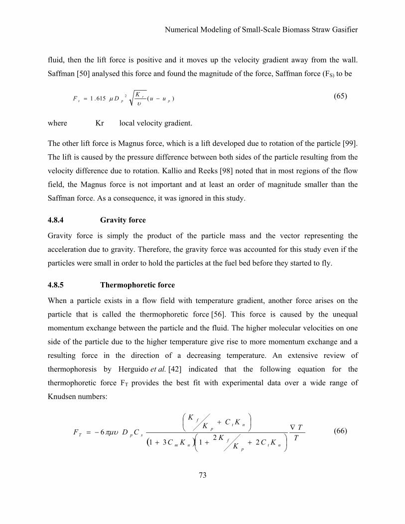
Numerical Modeling of Small-Scale Biomass Straw Gasifier
73
fluid, then the lift force is positive and it moves up the velocity gradient away from the wall.
Saffman [50] analysed this force and found the magnitude of the force, Saffman force (FS) to be
)(615.1 2p
rps uu
KDF −=
υμ (65)
where Kr local velocity gradient.
The other lift force is Magnus force, which is a lift developed due to rotation of the particle [99].
The lift is caused by the pressure difference between both sides of the particle resulting from the
velocity difference due to rotation. Kallio and Reeks [98] noted that in most regions of the flow
field, the Magnus force is not important and at least an order of magnitude smaller than the
Saffman force. As a consequence, it was ignored in this study.
4.8.4 Gravity force
Gravity force is simply the product of the particle mass and the vector representing the
acceleration due to gravity. Therefore, the gravity force was accounted for this study even if the
particles were small in order to hold the particles at the fuel bed before they started to fly.
4.8.5 Thermophoretic force
When a particle exists in a flow field with temperature gradient, another force arises on the
particle that is called the thermophoretic force [56]. This force is caused by the unequal
momentum exchange between the particle and the fluid. The higher molecular velocities on one
side of the particle due to the higher temperature give rise to more momentum exchange and a
resulting force in the direction of a decreasing temperature. An extensive review of
thermophoresis by Herguido et al. [42] indicated that the following equation for the
thermophoretic force FT provides the best fit with experimental data over a wide range of
Knudsen numbers:
( ) TT
KCKKKC
KCKK
CDFnt
p
fnm
ntp
f
spT∇
⎟⎠⎞
⎜⎝⎛ +++
⎟⎠⎞
⎜⎝⎛ +
−=22131
6πμυ (66)

Numerical Modeling of Small-Scale Biomass Straw Gasifier
74
where Kp particle thermal conductivity Kn Knudsen number ∇T temperature gradient Cs = 1.17 Ct = 2.18 Cm = 1.14
However, for particles considered here in this study, thermophoretic force could be neglected,
because the influence of other forces, such as the drag force, are much stronger for such small
particles of diameters less than 0.03 mm [107].
4.8.6 Brownian force
Brownian force is caused by random impact of the particle with agitated gas molecules [50]. For
submicron size particles, Brownian force could be quite important [79]. In particular, near solid
surfaces, where the intensity of turbulence becomes negligibly small, Brownian force could be
an important transport mechanism [98].
In previous work there was a general thinking that the Brownian force could dominate the
motion of submicron particles [48]. Recently, a clear model of the Brownian force and its effect
on particle trajectory was given by Ounis et al. [103]. They studied the Brownian dispersion of
submicron particles from a point source in a simulated turbulent channel flow field. The particle
equation of motion including the Brownian force was studied and ensembles of 8192 particle
trajectories were evaluated. The results are compared to those obtained from the exact solution of
the corresponding convective diffusion equation in the absence of turbulent fluctuations. It was
found in this work that the particles with diameters equal to or less than 0.03 μm were strongly
affected by turbulence, even those with a distance of one wall unit from the surface, and the
Brownian force could be neglected. Brownian force is not an important transport mechanism in
this region. Based on these results and since the particles considered in this study were larger
than 0.03 μm, the Brownian force was ignored.
4.9 Porous media model
The porous media assumption is generally used in the applications of biomass gasification in a
fixed bed [48]. The arrangement of biomass particles in the fixed bed forms void spaces. The

Numerical Modeling of Small-Scale Biomass Straw Gasifier
75
devolatilization volatiles and gases through the particle voids can be described as flow through a
porous media [84]. The particle position may change during the conversion process for the
devolatilization, combustion and shrinkage of biomass particles. In this process to mesh all
associated geometry with a complex unstructured or body fitted system was out of both
computational power and CFD algorithms a level [93].
Therefore, the simplified porous media assumption applies Darcy’s law to present the
relationship on pressure drop and volume averaged velocity caused by viscous drag [48]
υαμ
−=∇ p (67)
At high flow velocities, the modification of this law corrects for inertial losses in the porous
medium by the Darcy-Forchemier equation [48]
2υρυαμ
FCxp
+−=∂∂ (68)
Fluid flow, and heat and mass transfer are described in the sub-domain by the laws of
conservation of mass, momentum and energy in the terms of macroscopic variables and are
provided by the volume averaged Navier-Stocks equations in a version of Darcy’s law.
4.10 Discretization of the equations
Several methods have been employed over the years to solve the Navier-Stokes equations
numerically, including the finite difference, finite element, spectral element, and finite volume
methods [93]. The focus of the gasifier simulations is on the finite volume method, which is
described in detail below. Once this method and terminology are presented, the other methods
are briefly discussed.
To illustrate the discretization of a typical transport equation using the finite volume formulation,
a generalized scalar equation can be used with the rectangular control volume shown in
Figure 4.4. The scalar equation has the following form [56]:

Numerical Modeling of Small-Scale Biomass Straw Gasifier
76
( ) Sxx
Uxt ii
ii
′+⎟⎟⎠
⎞⎜⎜⎝
⎛∂∂
Γ∂∂
=∂∂
+∂
∂ φφρρφ )( (69)
The parameter Γ is used to represent the diffusion coefficient for the scalar Φ. If Φ is one of the
components of velocity, for example, Γ would represent the viscosity. All sources are collected
in the term S’. Again, if Φ is one of the components of velocity, S’ would be the sum of the
pressure gradient, the gravitational force, and any other additional forces that are present. The
control volume has a node, P, at its center where all problem variables are stored. The transport
equation describes the flow of the scalar Φ into and out of the cell through the cell faces [105].
To keep track of the inflow and outflow, the four faces are labelled with lower case letters
representing the east, west, north, and south borders. The neighbouring cells also have nodes at
their centres, and these are labelled with the capital letters E, W, N, and S. For the purpose of this
example, flow in the 1-D row of cells shown in Figure 4.4 was considered.
Figure 4.4: Simple 2-D domain showing the cell centres and faces (top), 1-D rectangular simplification (bottom) [109]
The first step in the discretization of the transport equation is integration over the control
volume. The volume integral can be converted to a surface integral by applying the divergence
theorem. Using a velocity in the positive x-direction, neglecting time-dependence, and assuming
that the faces e and w have area A, the integrated transport equation takes the following form
[61]:
Numerical Modeling of Small-Scale Biomass Straw Gasifier
77
SAdxd
dxdAUU
ww
eewwweee +⎟⎟
⎠
⎞⎜⎜⎝
⎛⎥⎦⎤
⎢⎣⎡Γ−⎥⎦
⎤⎢⎣⎡Γ=−
φφφρφρ )( (70)
where S is the volume integral of the source terms contained in S’. This expression contains four
terms that are evaluated at the cell faces. To obtain the face values of these terms as a function of
values that are stored at the cell centres, a discretization scheme is required.
4.10.1 Discretization schemes
Since all of the problem variables are stored at the cell centre, the face values (the derivatives,
for example) need to be expressed in terms of cell centre values [51]. To do this, consider a
steady-state conservation equation in one dimension without any source terms:
⎟⎠⎞
⎜⎝⎛
∂∂
Γ=xdx
ddx
Ud φφρ )( (71)
This equation can be solved exactly. On a linear domain that extends from x = 0 to x = L,
corresponding to the locations of two adjacent cell nodes, with Φ = Φ 0 at x = 0 and Φ = Φ L
at x = L, the solution for Φ at any intermediate location (such as the face) has the form [51]
( )1exp
1exp)(
−
⎟⎠⎞
⎜⎝⎛ −
−+=e
e
oL PLxP
φφφφ (72)
The Peclet number, Pe, appearing in this equation is the ratio of the influence of convection to
that of diffusion on the flow field and is given by [96]:
Γ=
ULPeρ (73)
Depending on the value of the Peclet number, different limiting behaviour exists for the variation
of Φ between x = 0 and x = L [48]. These limiting cases are discussed below, along with some
more rigorous discretization, or differencing schemes that are popular today.

Numerical Modeling of Small-Scale Biomass Straw Gasifier
78
a. Central differencing scheme
For Pe = 0, there is no convection, and the solution is purely diffusive [48]. This would
correspond to heat transfer due to pure conduction, for example. In this case, the variable Φ
varies linearly from cell centre to cell centre, so the value at the cell face can be found from
linear interpolation. When linear interpolation is used in general, i.e. when both convection and
diffusion are present, the discretization scheme is called central differencing [71]. When used in
this manner, as a general purpose discretization scheme, it can lead to errors and loss of accuracy
in the solution [109]. One way to reduce these errors is to use a refined grid, but the best way is
to use another differencing scheme. There is one exception to this rule. Central differencing is
the preferred discretization scheme when the large-eddy simulation (LES) turbulence model is
used [98].
b. Upwind differencing schemes
For Pe >> 1, convection dominates, and the value at the cell face can be assumed to be identical
to the upstream, or upwind value, i.e. Φ w = ΦW [98]. When the value at the upwind node is used
at the face, independent of the flow conditions, the process is called first order upwind
differencing [96]. A modified version of first order upwind differencing makes use of multi-
dimensional gradients in the upstream variable, based on the upwind neighbour and its
neighbours [84]. This scheme, which makes use of a Taylor series expansion to describe the
upwind gradients, is called second order upwind differencing [109]. It offers greater accuracy
than the first order upwind method, but requires additional computational effort [92].
c. Power law differencing scheme
For intermediate values of the Peclet number, 0 < Pe < 10, the face value can be computed as a
function of the local Peclet number, as shown in Equation (73) [98]. This expression can be
approximated by one that does not use exponentials, involving the Peclet number raised to an
integral power [96]. It is from this approximate form that the power law differencing scheme
draws its name. This first order scheme is identical to the first order upwind differencing scheme
in the limit of strong convection, but offers slightly improved accuracy for the range of Peclet
numbers mentioned above [90].

Numerical Modeling of Small-Scale Biomass Straw Gasifier
79
d. QUICK differencing scheme
The QUICK differencing scheme is similar to the second order upwind differencing scheme,
with modifications that restrict its use to quadrilateral or hexahedral meshes [105]. In addition to
the value of the variable at the upwind cell center, the value from the next upwind neighbour is
also used. Along with the value at the node P, a quadratic function is fitted to the variable at
these three points and used to compute the face value [84]. This scheme can offer improvements
over the second order upwind differencing scheme for some flows with high swirl [71].
4.11 Discretization of the domain
To break the domain into a set of discrete sub-domains, computational cells, or control volumes,
a grid is used [81]. Also called a mesh, the grid can contain elements of many shapes and sizes.
In 2-D domains, for example, the elements are usually either quadrilaterals or triangles. In 3-D
domains, they can be tetrahedral (with four sides), prisms (five sides), pyramids (five sides) or
hexahedral (six sides) (Figure 4.5).
Figure 4.5: Elements used as computational grids [109]
A series of line segments (2-D) or planar faces (3-D) connecting the boundaries of the domain
are used to generate the elements. Structured grids are always quadrilateral (2-D) or hexahedral
(3-D), and are such that every element has a unique address in I, J, K space, where I, J, and K are

Numerical Modeling of Small-Scale Biomass Straw Gasifier
80
indices used to number the elements in each of the three computational directions as shown in
Figure 4.6.
Figure 4.6: Structured grids in 2-D and 3-D with I, J and K directions [109]
The I, J, and K directions can, but need not be aligned with the coordinate directions x, y, and z.
Unstructured grids do not follow this addressing rule (Figure 4.7). Hybrid meshes are
unstructured meshes that make use of different types of elements (triangles and quadrilaterals,
for example). Block structured meshes use quadrilateral (2-D) or hexahedral (3-D) elements, and
have I, J, K structures in multi-cell blocks rather than across the entire domain.

Numerical Modeling of Small-Scale Biomass Straw Gasifier
81
Figure 4.7: Unstructured grids using hexahedral or mixture elements [109]
In general, the density of cells in a computational grid needs to be fine enough to capture the
flow details, but not so fine that the overall number of cells in the domain is excessively large,
since problems described by large numbers of cells require more time to solve [59]. Non-uniform
grids of any topology can be used to focus the grid density in regions where it is needed and
allow for expansion in other regions [99].
In laminar flows, the grid near boundaries should be refined to allow the solution to capture the
boundary layer flow detail. A boundary layer grid should contain quadrilateral elements in 2-D
and hexahedral or prism elements in 3-D, and should have at least five layers of cells [61]. For
turbulent flows, such as in the gasifier under investigation, it is customary to use a wall function
in the near-wall regions. Wall functions rely on the fact that the flow in a turbulent boundary
layer consists of a narrow viscous sub-layer and a broad, fully turbulent, or “log-law” layer in
which the behaviour is well documented [71]. In particular, the shear stress due to the wall can
be extracted from a linear relationship involving the log of the perpendicular distance to the wall.
This method will help to get the best possible predictions for pressure drop and heat transfer in
the simulation.
4.12 Solution methods
The result of the discretization process is a finite set of coupled algebraic equations that need to
be solved simultaneously in every cell in the solution domain. An iterative solution procedure
was required because the non-linearity of the equations that govern the fluid flow and related
processes [48]. Two methods are commonly used, namely the segregated and the coupled
approach [72]. A segregated solution approach is one where one variable at a time is solved
throughout the entire domain [71]. Thus the x-component of the velocity is solved on the entire
domain, and then the y-component is solved, and so on. An iteration of the solution is complete
only after each variable has been solved in this manner. A coupled solution approach, on the
other hand, is one where all variables, or at least, momentum and continuity, are solved
simultaneously in a single cell before the solver moves to the next cell, where the process is
repeated [98]. The segregated solution approach is popular for incompressible flows with

Numerical Modeling of Small-Scale Biomass Straw Gasifier
82
complex physics, typical of those found in mixing applications. For this reason, the segregated
approach will be implemented to solve the algebraic equations.
4.12.1 The SIMPLE and SIMPLEC algorithms
For 3-D simulations, the three equations of motion and the equation of continuity combine to
form four equations for the four unknowns that are the pressure and the three velocity
components [109]. Because there is no explicit equation for the pressure, special techniques have
been devised to extract it in an alternative manner. The most frequently used of these techniques
is the SIMPLE algorithm or Semi-Implicit Method for Pressure-Linked Equations [109]. Indeed,
a family of algorithm was derived from this basic one, which has a small modification that made
it well suited to one application or another called SIMPLEC [98].
The simulation has the following steps [51]:
1. Start the iterative process by guessing the pressure field. Denote the guessed pressure by
P'.
2. Use the values of p' to solve for u, v and w from the momentum equations. Since these
velocities are those associated with the values of p', denote these by u', v' and w'.
3. Since these values are obtained from guessed values of p', the values u', v', and w', when
substituted into the continuity equation, will not necessarily satisfy that equation.
Hence, using the continuity equation, a pressure correction p* is constructed, which when added
to p' brings the velocity field more into agreement with the continuity equation. That is the
corrected pressure p where p = p* + p'. Corresponding velocity corrections u', v', and w' can be
obtained from p' such that u = u* + u', v = v* + v' and w = w* + w'
4. For turbulent flows, solve turbulence model equations for k and e.
5. Designate the new value p on the left hand side in step 3 as the new value of p'.
Return to step 2, and repeat the process until a velocity field is found that satisfies the continuity
equation. When this is achieved, the correct flow field will be obtained.

Numerical Modeling of Small-Scale Biomass Straw Gasifier
83
SIMPLEC algorithms (see Figure 4.8 for the flow chart for the algorithm) are effective for
simple flows such as laminar flows where there are no additional submodels are activated.
Considering the complexity of the flow in the gasifier, the SIMPLE algorithm will give a better
chance for the solution to converge and avoid instability. Considering the complexity of the flow
in the gasifier, the SIMPLE algorithm will give a better chance for the solution to converge by
applying a lower under relaxation factor to stabilize the solution procedure [109].
Figure 4.8: SIMPLE algorithm chart [59]
4.12.2 PISO algorithm
The Pressure-Implicit with Splitting of Operators (PISO) pressure-velocity coupling scheme, part
of the SIMPLE family of algorithms, is based on the higher degree of the approximate relation
between the corrections for pressure and velocity [34].
One of the limitations of the SIMPLE and SIMPLEC algorithms is that new velocities and
corresponding fluxes do not satisfy the momentum balance after the pressure-correction equation
is solved [27]. As a result, the calculation must be repeated until the balance is satisfied. To

Numerical Modeling of Small-Scale Biomass Straw Gasifier
84
improve the efficiency of this calculation, the PISO algorithm performs two additional
corrections: neighbour correction and skewness correction. But for steady state problems, it does
not have a significant advantage over the SIMPLE or SIMPLEC algorithm [109].
4.13 Residuals
The total residual is the sum over all cells in the computational domain of the residuals in each
cell and is given by [34]
RRcellsP
p =∑,
(74)
Since the total residual, R, defined in this manner, depends on the magnitude of the variable
being solved, it is customary to either normalize or scale the total residual to gauge its changing
value during the solution process [34]. While normalization and scaling can be done in a number
of ways, it is the change in the normalized or scaled residuals that is important in evaluating the
rate and level of convergence of the solution [79].
4.14 Convergence criteria
The convergence criteria are preset conditions usually normalized or scaled for the residuals that
determine when an iterative solution is converged. One convergence criterion might be that the
total normalized residual for the pressure equation drop below 1 x 10⁻³ [96]. Another might be
that the total scaled residual for a species equation drop below 1 x 10⁻⁶ [79]. Alternatively, it
could be that the sum of all normalized residuals drop below 1 x 10⁻⁴ [96]. For any set of
convergence criteria, the assumption is that the solution is no longer changing when the
condition is reached, and that there is an overall mass balance throughout the domain. When
additional scalars are being solved (for example, heat and species), there should be overall
balances in these scalars as well.
4.15 Under relaxation
The solution of a single differential equation, solved iteratively, uses information from the
previous iteration. If Φn is the value of the variable from the previous iteration and Φn+1 is the
Numerical Modeling of Small-Scale Biomass Straw Gasifier
85
new value, then some small difference or change in the variable brings the variable from the old
value to the new one [98]. Rather than using the full computed change in the variable, ΔΦ it is
often necessary to use a fraction of the computed change when several coupled equations are
involved [59]. This process is called under relaxation, and under relaxation factors, f, typically
range from 0.1 to 1.0, depending on the complexity of the flow physics (laminar flow or
turbulent reacting flow, for example), the variable being solved (pressure or momentum), the
solution method being used, and the state of the solution (during the first few iterations or near
convergence) [93]. Under relaxation makes the convergence process stable, but slower.
Guidelines exist for the optimum choices for under relaxation factors for a variety of conditions.
As the solution converges, the under relaxation factors should be gradually raised to ensure
convergence that is both rapid and stable at all times. For the gasifier simulation, it was found
that relaxation factors around 0.3 were necessary to obtain a stable solution, of which the under
relaxation of the pressure equation was the most critical.

Numerical Modeling of Small-Scale Biomass Straw Gasifier
86
Chapter 5. Modeling Vidir Best gasifier
This section describes an analysis of the Vidir gasifier. At first, the simpler equilibrium model
with no spatial resolution was used to calculate gasification reactions. Once these results were
obtained, a fully resolved, spatial analysis was then performed for the gasifier using CFD.
5.1 Equilibrium model
The equilibrium model has been used by many researchers to analyse the gasification process.
Most models are based on minimizing Gibbs free energy [54, 101 and 105]. The understanding
of some mathematical theories is necessary for solving optimization and non-linear equation
problems. Another kind of equilibrium model is one based on an equilibrium constant.
Zainal et al. [91] used this type of equilibrium model to predict the composition of the producer
gas for different biomass materials. In this work, to develop the model, the chemical formula of
feedstock was defined as CHxOy. The global gasification reaction can be written as follows:
23.76mN4CHnO2Hn2CO
2COnnCO2H2Hn)23.76N2m(OO2ωHyOxCH +++++=−++ (75)
where x, y, z number of atoms of hydrogen, oxygen, and nitrogen per number
of atom of carbon in the feedstock
w amount of moisture per kmol of feedstock
m amount of oxygen per kmol of feedstock.
All inputs on the left side of Equation (75) are defined at 25oC. On the right side, ni are the
numbers of moles of the species i that are also unknowns.
Biomass fuels are characterized by the proximate and ultimate analyses [44]. They can be burned
directly for heat or to make steam for power. The proximate analysis gives moisture content,
volatile content usually when heated to 950oC, the free carbon remaining at that point, the ash
(mineral) in the sample, and the high heating value (HHV) based on the complete combustion of
the sample to carbon dioxide and liquid water [88]. The ultimate analysis gives the composition
of the biomass in wt% of carbon, hydrogen and oxygen that are the major components, and

Numerical Modeling of Small-Scale Biomass Straw Gasifier
87
sulfur and nitrogen if any [64]. The ultimate and proximate analyses of the biomass fuel were
used to obtain the fuel composition and the moisture content of the biomass. Table 5.1 shows the
ultimate and proximate analyses results table for wheat straw biomass used in the gasifier.
Table 5.1: Ultimate (a) and proximate analyses (b)
Sample Basis Moisture content
(%)
Ash (%)
Volatiles(%)
Fix Carbon
(%)
Caloric Value
(kJ/kg)
Wheat straw
As received
13.42 7.22 63.15 16.21 15632
Air dried 3.78 8.02 70.18 18.02 17373 Dry 0 8.34 72.94 18.73 18055
Sample Basis Moisture (%)
C (%)
H (%)
Ash (%)
N (%)
O (%)
Wheat straw
As received
13.42 40.81 4.48 7.22 0.94 33.01
Air dried 3.78 45.36 4.98 8.02 1.04 36.69 Dry 0 47.14 5.18 8.34 1.08 38.13
To find the five unknown species of the producer gas, five equations were required. Those
equations were generated using mass balance and equilibrium constant relationships.
Considering the global gasification reaction in Equation (75), the first three equations were
formulated by balancing each chemical element as shown in Equations (77) to (79).
Carbon balance
10421 −++== CHCOCO nnnf (77)
Hydrogen balance
wxnnnf CHOHH 242204222 −−++== (78)
Oxygen balance

Numerical Modeling of Small-Scale Biomass Straw Gasifier
88
ymwnnnf OHCOCO −−−++== 220223 (79)
Chemical equilibrium is usually explained either by minimization of Gibbs free energy or by
using an equilibrium constant. To minimize the Gibbs free energy, constrained optimization
methods are generally used [68]. The model in this study was based on thermodynamic
equilibrium and equilibrium constant was used instead of the Gibbs free energy to avoid
complicated mathematical theories that go with this approach [77]. The remaining two equations,
were obtained from the equilibrium constant of the reactions occurring in the gasification zone,
shown below:
Water-gas shift reaction
CO +H2O = CO2 + H2 (80)
Methane reaction:
C +2H2 = CH4 (81)
Higman and Van der Burgt [72] presented that Equation 80 can be created by combining the
Boudouard and water-gas reaction.
For the 1-D model in this study, the thermodynamic equilibrium is assumed for all chemical
reactions in the gasification zone. All gases were assumed to be ideal and all reactions took place
at a pressure of 1 atm. From Equations (80) and (81), the relationship between the equilibrium
constant, K, and mole of chemical species in each equation can be written as [91]
))(())((022214 HCOOHCO nnnnKf −== (82)
))(()(042
225 totalCHH nnnKf −== (83)
where K1 and K2 are equilibrium constant of the water-gas shift reaction and methane reaction,
respectively.
Equation (84) [91] is used for the equilibrium state of ideal gas mixture because of the
requirements of K1 and K2 values.

Numerical Modeling of Small-Scale Biomass Straw Gasifier
89
TRGK
oTΔ
−=ln , oiTf
ii
oT gG ,,Δ=Δ ∑υ (84)
R is the universal gas constant, 8.314 kJ/ (kmol⋅K), ΔGT is the standard Gibbs function of
reaction, and Δgfr represents the standard Gibb function of formation at a given temperature T of
the gas species i which can be expressed by the empirical equation below [84]:
TgfT
eKTdTcTbTTahg of
oTf ′+′+⎟
⎠⎞
⎜⎝⎛ ′
+⎟⎠⎞
⎜⎝⎛ ′
−⎟⎠⎞
⎜⎝⎛ ′
−′−′−=Δ232
)ln( 2432
, (85)
The values of coefficients a’ to g’ and the enthalpy of formation of the gases are presented in
Table 5.2 [84].
Table 5.2: The value hf (kJ/mol) and the coefficients of empirical equation for ΔgfT (kJ/mol)
Compound ofh
a’ b’ c’ d’ e’ f’ g’
CO -1.105
E+02
5.619
E-03
-1.190
E-05
6.383
E-09
-1.846
E+12
-4.891
E+02
8.684
E-01
-6.131
E+02
CO2 -3.935
E+02
-1.949
E-02
3.122
E-05
-2.448
E-08
6.946
E-12
-4.891
E+02
5.270
E+00
-1.207
E-01
H2O -2.418
E+02
-8.950
E-03
-3.672
E-06
5.209
E-09
-1.478
E-12
0.000
E+00
2.868
E+00
-1.722
E-02
CH4 -7.480
E+01
-4.620
E-02
1.130
E-05
1.319
E-08
-6.647
E+12
-4.891
E+02
1.411
E+01
-2.234
E+01
The temperature of the gasification zone needed to be calculated to calculate the equilibrium
constants (Equations 84 and 85). For this reason, the energy balance or enthalpy balance was
performed for the gasification process, which was assumed to be adiabatic as used
in reference [91]. When the temperature in the gasification zone is T and the temperature at the
inlet state is assumed to be 298 K (25oC), the enthalpy balance for this process can be written
as [76]

Numerical Modeling of Small-Scale Biomass Straw Gasifier
90
( )∑∑==
Δ+=prodi
iTofii
reactj
ofj hhnh ,
(86)
where hf enthalpy of formation in kJ/kmol and its value is zero for all
chemical elements at reference state (298 K, 1 atm)
ΔhT represents the enthalpy difference between any given state and at
reference state. It can be approximated by [97]:
32
298
)(,)( dTCTbTaTCdTTCTh p
T
pT +++==Δ ∫ (87)
where CP (T) is specific heat at constant pressure in kJ/kmol K and it is a
function of temperature.
a, b, c, and d are the specific gas species coefficients, which are shown in
Table 5.2.
Equation 86 can be rewritten as [91]:
⎥⎦
⎤⎢⎣
⎡+⎟
⎠
⎞⎜⎝
⎛+⎟
⎠
⎞⎜⎝
⎛+⎟
⎠
⎞⎜⎝
⎛+⎟
⎠
⎞⎜⎝
⎛+= ∑∑∑∑∑∑∑
== iii
iii
iii
iiiii
i
ofi
prodii
reactj
ofj knTdnTcnTbnTanhnh 432 (88)
where κ is a constant obtained from the integration. Sharma [48] suggested the relationship for
finding the enthalpy of formation for solid fuel in reactant that is:
( )( )kfkprodk
offuel hnLHVh 0∑
=
+= (89)
where hfk enthalpy of formation of product k under complete combustion of
the solid fuel
LHV lower heating value of the solid fuel in kJ/kmol.
The temperature in the gasification zone can now be calculated from Equation (88) using the
Newton-Raphson method. This relationship can predict the reaction temperature by knowing the

Numerical Modeling of Small-Scale Biomass Straw Gasifier
91
amount of oxygen. This makes the model a good tool to show the variation of reaction
temperature when a mole of oxygen is changed.
To solve the values of nH2, nCO, nCO2, nH2O and nCH4, an initial temperature was assumed and
substituted into Equations (84) and (85) to initially calculate K1 and K2. Then, both equilibrium
constants were substituted into Equations (82) and (83), respectively. Finally, all five equations
i.e. Equations 77, 78, 79, 82, and 83 were used and solved simultaneously by the Newton-
Raphson method [95]. For calculating the new value of temperature, Equation (88) was used.
The outlined procedure is repeated again until the temperature value converged.
To verify the equilibrium model, a stoichiometric calculation spread sheet developed by Langner
[100] that implements the equilibrium model was used for conditions in the Vidir gasifier. A
sample of results of the mass and energy balance is shown on Table 5.3 and 5.4, respectively. In
addition, the results from these calculations were used to make sure the predictions from the
3-D model were consistent overall with the equilibrium gasification model.
Table 5.3: Sample mass balance equilibrium model results
Mass in Mass out C 0.402 0.402 H 0.078 0.078 O 1.389 1.389 N2 2.999 2.999 Ash 0.042 0.042 Other 0.000 0.000 Total 4.910 4.910 Mass in Mass out Air 3.910 0.000 Fuel 1.000 0.000 Syngas 0.000 4.869 Ash + trace 0.000 0.042 Total 4.910 4.910

Numerical Modeling of Small-Scale Biomass Straw Gasifier
92
Table 5.4: Sample energy balance equilibrium model results
Energy in (kW) Energy out (kW) Air 0.00000 H2 317.37
Fuel -5522.77 CO -737.62 Moisture -1699.93 CO2 -6535.60
H2O(g) -5697.46 CH4 0.06945 N2 5430.54
Total -7222.71 Total -7222.71
5.2 Simulation environment
This Vidir gasifier simulation was performed using the computational fluid dynamics software
Fluent® 6.2 code which is licensed by Fluent® Inc. Fluent® 6.2 is a computer program for
modeling fluid flow and heat transfer in complex geometry [93]. It provides mesh flexibility, as
it solves fluid flow problems using structured and unstructured grid that can be generated for
complex geometry with relative ease. Gambit® 2.4 from Fluent Inc. was used for the geometry
set-up and mesh generation. Gambit® 2.4 is a pre-processor for geometry modeling, block-
structured mesh generation and unstructured triangular surface mesh generation in two and three
dimensions [109]. All simulations were performed on a PC computer equipped with two
processors AMD Opteron Processor 240, 1.40 GHz, and 2 GB main memory system located at
the Wind Tunnel Lab, University of Manitoba. The same Fluent 6.2 CFD commercial software is
used to specify physical models, boundary conditions, and fluid properties in the computational
domain. All the computations were performed assuming steady-state conditions.
5.3 Model set up
5.3.1 Geometry/ mesh generation
Fluent® 6 has a two-part package consisting of a pre-processor, Gambit®, and a main module,
Fluent® [109]. Gambit® 2.4 was used to create the geometry and generate structural grids, and the
triangular grids were developed to efficiently model the complex geometries of the gasifier (for
detailed dimensions of the gasifier in this study, refer to Appendix A). Special attention was paid

Numerical Modeling of Small-Scale Biomass Straw Gasifier
93
to developing meshes that represent known areas of known high gradients. Several different,
three dimensional grids were investigated involving the initial use of tetrahedral grids, but finally
converged to the use of hexahedral grids as much possible, despite the difficulty of adapting such
a grid to the highly complex configuration of the gasifier. Figure 5.1 shows the typical grid for
the cases studied.
5.3.2 Boundary conditions
The inlet air flow was assumed to be incompressible, vertically uniform in speed, and all the
computations were performed assuming steady-state conditions. The problem taken up in this
study had three types of boundaries: inlet, outlet, and the wall. These boundary conditions were
prescribed in the following ways.
Figure 5.1: Gasifier grid
a. Inlet boundary
The mass flow rate boundary condition was used to define the inflow with all relevant scalar
properties of the flow at the primary air, secondary air and fuel port flow inlets. The mass flow
rate and direction, and the velocity magnitude normal to the boundary were specified. The mass
flow rates used as a base case in the present study were 0.24, 0.65 and 0.05 kg/s to primary,

Numerical Modeling of Small-Scale Biomass Straw Gasifier
94
secondary air inlets and fuel port respectively. These values were obtained from the data log
gasification of wheat straw in the Vidir Best gasifier.
b. Outlet boundary
The outlet boundary condition was used to model the flow at exit where the details of the flow
velocity and pressure were not known prior to solving the problem. Because these variables were
not known for the case under study, the outlet boundary condition was applied to the secondary
chamber exit. When this condition was specified, the code extrapolated the required information
from the interior. In the present study, since there was only one outlet, the flow rate weighting
was set to one to indicate that the whole fraction of total flow rate takes place in this boundary.
c. Wall boundary
In any flow, Reynolds number of the flow becomes low and turbulent fluctuations are damped
considerably near the walls where the laminar viscosity starts to play a significant role. In the
present case, walls were assumed to be adiabatic with no-slip condition. The standard wall
functions were used to calculate the variables at the near wall cells and the corresponding
quantities on the wall.
The temperature gradients in axial and circumferential directions are much smaller than that in
radial direction [53]. It was therefore considered that heat was transferred radially. The
conduction heat transfer through the multi-layer wall of the cylindrical vessel can be calculated
by the following equation [48]:
∑−
=
ii
outWinWcond R
TTQ
,
,,
λ (90)
where TW,i inside wall temperature, K
TW,out outside wall temperature, K
Rl, heat resistance of i th layer, K/W

Numerical Modeling of Small-Scale Biomass Straw Gasifier
95
Lrr
Ri
iin
iout
i πλλ 2
ln,
,
, = (91)
where rout,I outside radius of ith layer, m
rin,i inside radius of ith layer, m
L height of the cylinder, m
λi thermal conductivity of ith layer, W/ (m K)
The heat transfer from the outside wall to ambience includes the heat convection and the heat
radiation as follows [53]:
)T(TL σσ2 ππ)T(TLh2 ππQ 4am
4outW,outoutamoutW,outoutout −+−= (92)
where rout outside radius of the cylinder, m
hout convection heat transfer coefficient outside cylinder, W/
(m2 K)
Tam ambient air temperature, K
Σ Stefan-Boltzmann constant, 5.67 x 10⁻⁸ W/ (m2 K4)
εout emissivity of outside wall
The heat transfer on the inside wall includes three parts: convection heat transfer between
combustion gas and the wall, radiation heat transfer from combustion gas to the wall, and
radiation heat transfer from the wall to combustion gas [48].
4,2 inWinininnet TLrQQ σεπ−=
(93)
where, Qnet net heat transfer to the wall refractory, W
Qin sum of convection and radiation heat transfer from
combustion gas to the wall, W
rin inside radius of the cylinder, m
εin emissivity of inside wall

Numerical Modeling of Small-Scale Biomass Straw Gasifier
96
5.3.3 Porosity and bed height
A packed bed is an assembly of individual particles and consists of a solid phase (the particles)
and the gas phase (gases flowing through the gaps between the particles). It is difficult to
measure airflow velocity within the porous media straw in the gasification chamber. The
common practice is to measure the static pressures in a cylinder to establish an airflow
distribution profile because the pressure differences at two points cause airflow [48]. Based on
this fact, since the straw had a non-homogenous structure, it would cause an uneven pressure
distribution in both horizontal and vertical direction, within itself. This type of pressure
distribution will cause non-uniform airflow in return. Thus, horizontal pressure distribution is
determined in a central plane of a wheat straw bed to study the uniformity of airflow. The
rationale for choosing the central plane was because the central plane was the plane separating
the straw into equal parts subjected to equal sensitivity to pressure changes at either part of the
bed.
The schematic of the experimental setup is shown in Figure 5.2. A cylindrical vessel was used to
place the straw. This cylinder represented the primary chamber of an updraft gasifier (the
primary chamber of the Vidir Best), in which the gasification occurs. The bottom of the vessel
was covered with a screen to hold the straw but allowed air to flow upward. Its height and
diameter were 100 and 50 cm, respectively. Four taps are arranged with the same height from the
bottom to measure the static pressure values in the same central plane.
Straw was loaded into the vessel by hand shovel and leveled by hand from time to time without
compressing. After the depth of the straw bed reached 80 cm, air was supplied to the bottom of
the vessel at the superficial velocity of 0.175 m3/s m2. The superficial velocity in a single phase
flow equals its mean velocity, while in multiphase flows is defined as the ratio of the velocity
and the volume fraction of the considered phase in a multiphase system [78]. An even pressure
was provided from the bottom and calibrated orifices were used to measure airflow. Static
pressure values in the central plane of the straw bed are measured by using probes made from
steel tube. The probe was connected to a digital manometer whose range and resolution were
± 249 Pa and ± 0.25 Pa, respectively. The probes were inserted through the pressure taps into the
can and duct tape is used to seal the space between the probe and the tap. The pressure readings

Numerical Modeling of Small-Scale Biomass Straw Gasifier
97
were taken through the four taps 80, 90 and 100 cm from the bottom of the can for different
angles and distances from the walls. In addition, the pressure drop across the packed bed was
measured by a differential U-tube manometer. Two tests were done using wheat straw with low
aspect ratio (the ratio of the largest to the smallest dimension of the particle) and cattail with
large cylindrical particles having the highest aspect ratio that is the ratio of width to height
biomass [29].
It was observed that the porosity of the wheat straw was 0.4333, while the cattails had the
highest porosity equal to 0.5409. The wheat straw particles were found to be in close surface-to-
surface contact among them, leading to a higher packing density, while cattail particles were
found to have more inter-particle branching, thus contributing to a higher observed porosity.
Figure 5.2: Experimental schematic
The results showed significant absolute pressure deviations, which indicated non-uniform
airflow distribution existed in the central plane of the straw bed (Figure 5.3). A pressure
deviation closer to the inner surface of the vessel was observed. The reason for this might have
been the presence of an edge effect. Edge effect is the occurrence of lower straw bed density

Numerical Modeling of Small-Scale Biomass Straw Gasifier
98
closer to the inner surface of the reactor, since straw particles could not settle down near the
edges because of their long sizes [68]. Therefore, air flowed more easily near the edges of the
gasifier because of lower bed densities. Based on this observation one can conclude that a wide
straw size distribution resulted in a reduction of uneven airflow distribution. The angle effect on
the pressure deviation might have been caused by the uncontrollable factors associated with
straw loading by hand-shovel. The results of these experiments (Figure 5.3) were used to model
the straw bed.
Figure 5.3: Pressure drop as a function of air velocity for straw
5.3.4 General description of model
The gasifier operated in atmospheric condition and air was used as the oxidizing agent. Wheat
straw which was used as biomass was characterized using the main energetic parameters such as
higher heat value, chemical characteristics (carbon, hydrogen and nitrogen content), physical
parameters (moisture, ash and volatile compounds) based on the ultimate and proximate analysis
(Table 5.1). Finally, first order discretization method was used coupled with the k-ε model of
turbulence. A typical hexahedral three dimensional grid of the gasifier under investigation with
the corresponding boundary conditions are shown below in Figure 5.4.
The k-ε turbulence model was implemented with to an eddy-viscosity model in which the
Reynolds stresses were assumed to be proportional to the mean velocity gradients, with the
constant of proportionality being the turbulent eddy viscosity. The turbulent viscosity was

Numerical Modeling of Small-Scale Biomass Straw Gasifier
99
assumed to be proportional to the product of a turbulent velocity scale and length scale. In the κ-
ε model, these velocity and length scales were obtained from two parameters: the turbulent
kinetic energy (k), and the dissipation rate (ε).
The closure coefficients and auxiliary relations used for the κ-ε model were obtained from
Launder et al. [40], where the empirical turbulence coefficients within the dissipation rate term
are defined as Ce1 = 1.44 and Ce2 = 1.92.
The governing equations in the transformed coordinates were discretised using the finite volume
technique. Finite volume discretization is a numerical method approach of solving partial
differential equations instead of using an analytical method. The domain over which the
dependent variable was to be evaluated was broken into a finite number of discrete volumes and
algebraic equations were written for each volume. A numerical solution of a differential equation
consists of a set of numbers from which the distribution of the dependent variable is then
constructed. The pressure velocity coupling was numerically implemented using the SIMPLE
algorithm which is basically an iterative approach, where some innovative physical reasoning is
used to construct the next iteration from the results of the previous iteration.
Figure 5.4: Boundaries of gasifier

Numerical Modeling of Small-Scale Biomass Straw Gasifier
100
Close to solid walls, there are boundary layer regions where the local Reynolds number is so
small that viscous effects predominated over turbulent effects [71]. To account for this effect and
for the large gradients of variables near the wall, the wall function method of Launder and
Spalding [40] was used in the CFD model.
Thermal boundary conditions were defined at all the fluid inlets and at all the wall/fluid
interfaces in the computational domain. At the fluid inlet, the air temperature, mass flow rate,
direction, atmospheric pressure, gravitational acceleration, turbulence intensity, and hydraulic
diameter were specified. The thermal conditions of density, specific heat, viscosity, and thermal
conductivity were also specified for the fluid inlets. For the walls, several thermal boundary
conditions are specified such as surface temperature, emissivity of the wall, and conductive heat
transfer coefficient.
The arrangement of biomass straw in the fixed bed of the gasifier formed void spaces through
which the primary air flowed through. Therefore, devolatilization volatiles and gases through the
bed could be approximated to be described and modelled as flow through a porous media. Fluid
flow, and heat and mass transfer are described in the sub-domain by the laws of conservation of
mass, momentum and energy in the terms of macroscopic variables provided by the volume
averaged Navier-Stocks equations in a version of Darcy’s law [48]. The bottom of the primary
chamber where the straw rests was defined as porous media zone. One of the parameters when
dealing with a packed bed is the porosity. Observation of the actual gasifier operating indicated
the partial presence of more molten-like biomass at the centre of the bed. The biomass had lost
the packed wheat straw appearance, which resulted in a variation of porosity as a function of
radial distance. Molten biomass resulted in more resistance to the air flow, and hence exhibited
low porosity. Therefore, the porosity of the bed was expected to be high going outward from the
centre. To account for this variation a User Defined Function (UDF) was implemented relating
the porosity as a function of radial distance in Fluent. The fact that the distribution was linear has
also confirmed by doing an experiment and the correlation obtained from the experiment was
used in developing the UDF function for the porosity (see Section 5.3.3).
In addition, a better understanding of the conditions in the bed was required to allow prediction
of the gas composition to be predicted at the bed/freeboard interface. The fact that the bed was a

Numerical Modeling of Small-Scale Biomass Straw Gasifier
101
pile of straw with elongated particles stacked on each other makes it difficult to accurately
model. To tackle this short coming, the method of holding straw elongated particles stationary on
the fuel bed became important. UDF developed by Langner [100] that keep the straw particle on
the bed until they lose their weight by evaporation and thermal conversion was used. These UDF
set the drag coefficient to a minimum value and applied a body force to counteract the gravity
force. Once they were held stationary, evaporation, devolatization and combustion allowed them
to lose weight. A 4.5% of initial mass loss of the particles was set as a threshold limit for the
particles before they could be entrained by the flow (Stoke flow), as suggested by Langner [100].
The flow in the biomass gasifier was a typical type of gas-solid flow with chemical reactions
found in many processes. Thus, hydrodynamics of the gas-solid flow was performed based on
the Eulerean–Lagrangian concept [111]. The discrete phase method was applied to the particle
flow since the particle phase could be considered to be sufficiently dilute that the particle-particle
interactions and the effects of the particle volume fraction on the gas phase could be
neglected [91]. The coupling of the continuous phase and the discrete phase was important and it
was solved by tracking the exchange of mass, momentum and energy.
Species transport model was implemented to simulate the transport and chemical reactions of
eight species namely O2, H2, H2O, CO, CO2, CH4, Straw-volatile and N2. A total of eight mixture
species with five reactions are modelled (detail in Appendix A). The properties of the individual
species are applied accordingly. Specifying dependencies of the properties of the medium on
temperature was also taken into account. When simulating fluid flows with heat transfer, as
source data, laws of variation of physical properties of the medium (density, viscosity, specific
heat conductivity, heat capacity) on the temperature needed to be specified properly. These
properties were specified using polynomial smooth functions. Thus, for computing properties at
certain temperature, piecewise-linear approximation is used.
A detailed summary of the boundary conditions, materials and their properties and sub-models
used are given in Appendix A.

Numerical Modeling of Small-Scale Biomass Straw Gasifier
102
5.4 Base case results
Proper set-up of the parameters of the experiment impacted the accuracy of the calculation as
compared to the real gasifier. The main groups of parameters were the dimensional parameters
defined by the grid, the material properties defined in the entries and the boundaries conditions
defined both by the grid and the boundary entries. Three meshes were evaluated from 500,000 to
1,000,000 elements for grid independence. The limits required for these calculations were to
obtain residuals less than 10-5. This required equilibrium between the computational time and the
accuracy of the parameters. Even when the residuals went below the set levels it was not
guaranteed that the solution had converged. Therefore, in addition to the convergence criteria set
up, a check to know whether the solution had converged was done by monitoring the mass flow
rate at the outlets. When the mass flow rate at outlet did not vary significantly with the iterations
and the residuals were less than 10-5, the solution was taken as converged. The grid used for this
case was 1,000,457 elements. This choice allowed for reaching the convergence of the results
after 120 to 130 hours and 18,000 to 19,000 iterations for the 3-D gasifier geometry shown in
Table 5.5.
Table 5.5: Mesh density dependence for equilibrium gasifier outlet temperature [K]
Mesh density Temperature (K)
Temperature from Fluent
(K)
Time to converge (Hours)
Percentage error (%)
500,000 1,165 689 24 40.85 600,000 1,165 785 35 32.61 700,000 1,165 846 47 27.38 800,000 1,165 923 59 20.77 900,000 1,165 1109 83 4.80 1,000,000 1,165 1123 128 3.60 1,200,000 1,165 1125 147 3.43 1,500,000 1,165 1126 195 3.33
The gasifier used as a base case had a secondary air inlet nozzle configuration of 90 degree (see
Section 5.3.1 for geometry and Section 5.6.2 for alternative configurations). The primary and
secondary air inlet mass flow rates were 0.24 kg/s and 0.65 kg/s, respectively (see Section 5.3.2

Numerical Modeling of Small-Scale Biomass Straw Gasifier
103
where the geometry of inlet air is described). The total air was set to produce an excess air ratio
of 40%, consistent with gasifier control operations for the base case. The wheat straw used for
the gasification model had moisture content of 14% as measured.
At the beginning of the simulation the fuel and air was set to a uniform temperature as an initial
guess and the volatiles were released from the straw and began to combust releasing heat as
shown in Figure 5.5. The moisture in the fuel started to leave once the boiling temperature was
reached, which resulted in a rapid increase of the molar fraction of water vapour and a
corresponding decrease of the molar fraction of oxygen and nitrogen, because of the dilution
caused by the released water vapour.
An immediate combustion took place at the bottom of the bed where the levels of available
oxygen were highest. Due to exothermic combustion reaction, the temperature of the bed rapidly
increases. At this stage, the O2 level was dropped and a sharp increase in CO mass fraction was
predicted. The local gas compositions remained at high and stable levels for a relatively long
period of time. During this stage, the mass fractions of CO, H2 and CH4 reached their maximum
level. Later, as the simulation progressed and approached convergence, a sharp decrease in all
volatile fuel species occurred.
Figure 5.6 shows the velocity magnitude contours in the vertical plane at Z = 0 (midsection of
the gasifier) when the simulation has converged. It was observed that the velocity magnitude
inside the gasifier was generally low. In the upper region of the gasifier, where syngas left the
primary chamber, the gas velocity was higher compared with the region inside the chamber due
to the convergent section. The velocity vector plot in the vertical plane at Z = 0 is shown in
Figure 5.7. The gas velocity increased when gas passed through the connecting duct between the
primary (Figure 5.9) and secondary chamber, and when it left the secondary chamber through the
outlet tube (Figure 5.10).
The formation of recirculation flow regions at several locations in the gasifier can be seen in
Figures 5.8 to 5.10; the path of fuel particles is shown in Figure 5.11. The recirculation flow
zone increased the particle residence time, and the local intensity of gas turbulence and thus
contributes to the particle deposition rate. The presence of the recirculation flows could also lead

Numerical Modeling of Small-Scale Biomass Straw Gasifier
104
to the gradual buildup of ash in these regions. The temperature contour profiles are shown in
Figure 5.12. The maximum temperature was 1900 K located in the area next to the secondary air
inlet, which is consistent with gasifier operation and controls. The reason for the high
temperature spot is the result of the excess oxygen and reaction of CO. At the bottom of the
primary chamber, a low temperature zone was observed because this zone is the zone of
gasification. The mass fractions of gases are also shown in Figures 5.13 to 5.17.
Figure 5.5: Contours of mass fraction of straw volatiles at start of simulation
Figure 5.6: Contours of velocity magnitude once converged [m/s]
Bed Height

Numerical Modeling of Small-Scale Biomass Straw Gasifier
105
Figure 5.7: Velocity vectors colored by velocity magnitude at top of gasifier [m/s]
Figure 5.8: Contours of velocity magnitude near secondary air inlet [m/s]

Numerical Modeling of Small-Scale Biomass Straw Gasifier
106
Figure 5.9: Contours of velocity magnitude near secondary air inlet [m/s]: (x = 0 plane)
Figure 5.10: Contours of velocity magnitude near secondary chamber outlet [m/s]

Numerical Modeling of Small-Scale Biomass Straw Gasifier
107
Figure 5.11: Fuel path lines colored by particle ID
Figure 5.12: Contours of static temperature [K]

Numerical Modeling of Small-Scale Biomass Straw Gasifier
108
Figure 5.13: Contours of mass fraction of O2
Figure 5.14: Contours of mass fraction of CO2

Numerical Modeling of Small-Scale Biomass Straw Gasifier
109
Figure 5.15: Contours of mass fraction of H2O
Figure 5.16: Contours of mass fraction of H2

Numerical Modeling of Small-Scale Biomass Straw Gasifier
110
Figure 5.17: Contours of mass fraction of CO
5.5 Validation
The process of obtaining a converged solution was of critical importance in these numerical
simulations. To monitor this process, residuals for each equation and for each 100 iterations were
monitored during the simulation, with careful attention to the convergence of the energy equation
owing to the fourth order source terms, and resulting from the radiation dominated heat transfer
inside the gasifier [109]. The residuals are a measure of how closely each finite difference
equation is balanced, given the current state of the solution. Residuals for each conservation
equation were computed by summing the imbalance in the equation for all cells in the domain.
The residuals of the calculation, which represent the accuracy of the results, were less than 10-5 at
the end of the calculations for all parameters throughout the simulations.
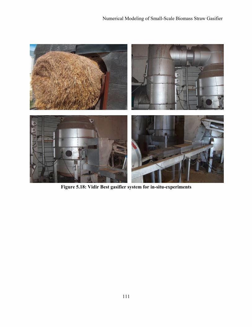
Numerical Modeling of Small-Scale Biomass Straw Gasifier
111
Figure 5.18: Vidir Best gasifier system for in-situ-experiments

Numerical Modeling of Small-Scale Biomass Straw Gasifier
112
Figure 5.19: In-situ particulate emission sampling
Once convergence was obtained with the proper mesh size, the temperatures in the primary and
secondary chamber from the simulation were compared to the experimental data obtained by
running the Vidir Best gasifier for validation. Details of the operating conditions for the base
case of the Vidir system for the gasification of the wheat straw can be found in Appendix F. The
results show that the temperature in the primary chamber was 900 K (1154.3oF) and the
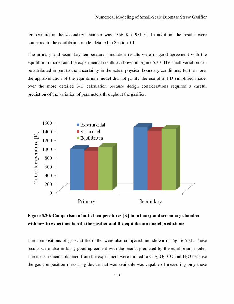
Numerical Modeling of Small-Scale Biomass Straw Gasifier
113
temperature in the secondary chamber was 1356 K (1981oF). In addition, the results were
compared to the equilibrium model detailed in Section 5.1.
The primary and secondary temperature simulation results were in good agreement with the
equilibrium model and the experimental results as shown in Figure 5.20. The small variation can
be attributed in part to the uncertainty in the actual physical boundary conditions. Furthermore,
the approximation of the equilibrium model did not justify the use of a 1-D simplified model
over the more detailed 3-D calculation because design considerations required a careful
prediction of the variation of parameters throughout the gasifier.
Figure 5.20: Comparison of outlet temperatures [K] in primary and secondary chamber
with in-situ experiments with the gasifier and the equilibrium model predictions
The compositions of gases at the outlet were also compared and shown in Figure 5.21. These
results were also in fairly good agreement with the results predicted by the equilibrium model.
The measurements obtained from the experiment were limited to CO2, O2, CO and H2O because
the gas composition measuring device that was available was capable of measuring only these

Numerical Modeling of Small-Scale Biomass Straw Gasifier
114
gases (see Appendix E for details). In addition, the experimental results had several possible
errors which were difficult to quantify: unsteady effects, uncertainties with the boundary
conditions measurements, and variations in a field value across a duct that could not be
accurately measured with small sampling volume. Only the hydrogen composition was not well
predicted which can most likely be attributed to the reaction kinetics used for hydrogen in the
model.
Figure 5.21: Comparison of mass composition of gases [%] with in-situ experiments with
the gasifier and the equilibrium model predictions
5.6 Design improvement for air control
The motivation to develop a 3-D model that captures the physical phenomenon and thermal-fluid
complexities occurring inside a small-scale gasifier is to be able to deviate from the base
configuration and develop a predictive tool to understand the expected behaviour based on a
given geometry or process change. As any changes cause variations in the flow, heat transfer
and chemical reactions, it is critical to use an approach that models the physics properly, or at
least one that incorporates up-to-date models that have been validated for the intended use.
Rather than use trial and error by building numerous prototypes and test these during expensive
O2 CO2 H2O CH4 H2 CO

Numerical Modeling of Small-Scale Biomass Straw Gasifier
115
demonstrations, or even worst, experiment with new designs using a client’s system, the ability
to predict changes will lower costs and allow optimizing the system over a shorter period of
time. For small-scale renewable energy applications, flexible modeling is a critical aspect
because access to capital is scarce and failures occurring during demonstrations and first time
commercialisations are rapidly known within the industry and to potential future customers. This
section investigates the effect of changing geometry and operating parameters for the gasifier.
These new configurations could not be validated because they were exploratory and were
necessary to develop an understanding of how best to improve the controls of the gasifier or
make changes to the geometry. The following were investigated where bolded values represent
the base case conditions previously described. This test matrix resulted in 10 new simulations to
investigate design variation from the base case.
Table 5.6: Summary of parameters investigated
Aspect Parameter varied Comparison to base case
Moisture content
Moisture content (14%, 20%, 26%) Velocity magnitude (more water), secondary chamber temperature, calorific content, mass fraction of gases
Nozzle configuration
Angle of secondary air nozzle (30º, 45º and 90º )
Velocity magnitude, recirculation
Secondary to primary ratio (Primary air flow rate)
Primary air flow rate (0.16, 0.25 and 0.35 kg/s); secondary stays the same
Pressure drop across fuel bed, velocity magnitude, mass fraction of gases
Fuel bed height
Straw bed height ratio to cylindrical part of primary chamber height (0.6, 0.7, 0.8)
Temperature, mass fraction gases
Biomass types
Composition of biomass fuel (wheat straw, slough hay and wood chip)
Velocity magnitude, secondary chamber temperature, mass fraction of gases

Numerical Modeling of Small-Scale Biomass Straw Gasifier
116
5.6.1 Moisture Content Variation
Moisture variation in wheat straw is difficult to control, especially for small scale gasifier
implementations. Large combustors burning straw have tight control on the biomass delivery
process, ensuring that bales are within specified moisture content. For the Vidir gasifier which
uses large 1,000-kg bales, it is unrealistic to assume that even within even a single bale the
moisture content can be controlled. Often a wet patch is found which cannot be detected with a
simple moisture measurement probe that is inserted only a few inches within a bale. The gasifier
control systems need to be able to react to a relatively large moisture variation. Small-scale
implementation of a gasifier cannot rely on the user to implement sophisticated feedstock
moisture controls.
To study the effect of moisture content of the biomass, the amount of primary and secondary air
was fixed at 0.24 and 0.65 kg/s and the moisture content of the wheat straw was varied from 20%
and 26%. Figures 5.22 and 5.23 show the effect of moisture content on the reaction temperature,
the calorific value, and the composition of producer gas. The temperature in the primary chamber
dropped from 900 oK at 14% MC to 800.9 oK when the moisture content increased to 26.0%. The
change in temperature in the secondary chamber decreased from 1356 K for the base case to
1324 K and 1280 K for a MC 20.0% and 26.0%, respectively (Figure 5.22). The calorific value
also dropped from 4.76 MJ/Nm3 to 4.55 MJ/Nm3 (Figure 5.23). Hence, moisture content
negatively affects the calorific value of producer gas and causes the temperature distribution
within the gasifier to vary, impacting the thermal conversion process of the fuel. The controller
therefore needs to react to this change by first noticing that the temperature in the chamber has
decreased and develop a mitigation strategy which can include a change in primary air, addition
of more fuel or implement flue gas recirculation.
The composition of gases variation as a result of the different moisture contents is shown in
Figure 5.24. The CO2 decreased from 11.0% to 6.0% with increasing moisture content while CH4
had a low percentage in the producer gas, though it showed an increase from 0.15% to 0.19%.
For O2, it decreased from 11.3% to 9.8%. In the case of CO2, an inverse tendency was shown by
the simulation results. In regards to composition of mass fraction of gases, shown in Figure 5.24,
the fraction of H2 increased from 1.4% to 1.9% when the moisture content increased from 14.0%

Numerical Modeling of Small-Scale Biomass Straw Gasifier
117
to 26.0%. The contour plots of velocity magnitude, temperature, and O2 are shown in Figures
5.25 to 5..27 for the three moisture contents under consideration.
The moisture content of the straw had an obvious influence on the operation of the gasifier:
increases in moisture content resulted in an increasing equivalence ratio and gas yield and
aberrant temperature fluctuations. When a biomass with high moisture content is used, an
increase in the air supplied to the system is required to keep the reaction temperature. However,
increasing the amount of air randomly causes disadvantages and one of them is the mass fraction
reduction of useful gases which consequently reduce the heating value of the syngas. Therefore,
a careful adjustment to get the optimum air supply has to be implemented to enhance the thermal
decomposition characteristics of the biomass, thus higher calorific value syngas is produced.
Figure 5.22: Effect of MC on caloric value of producer gas in primary chamber

Numerical Modeling of Small-Scale Biomass Straw Gasifier
118
Figure 5.23: Effect of MC on the secondary temperature [K]
Figure 5.24: Effect of MC on the producer gas composition
O2 CO2 H2O CH4 H2 CO

Numerical Modeling of Small-Scale Biomass Straw Gasifier
119
Figure 5.25: Contours of velocity magnitude [m/s] with variation in MC: a) 14%, b) 20% and c) 26%
(a)
(b)
(c)
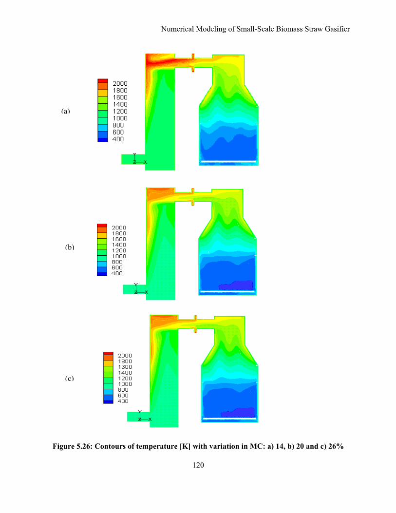
Numerical Modeling of Small-Scale Biomass Straw Gasifier
120
Figure 5.26: Contours of temperature [K] with variation in MC: a) 14, b) 20 and c) 26%
(a)
(b)
(c)

Numerical Modeling of Small-Scale Biomass Straw Gasifier
121
Figure 5.27: Contours of mass fraction of O2 with variation in MC: a) 14%, b) 20% and c) 26%
(a)
(b)
(c)

Numerical Modeling of Small-Scale Biomass Straw Gasifier
122
5.6.2 Nozzle configuration
The velocity field and the combustion reaction pattern in the secondary chamber are governed by
configuration of air injection nozzles, which represents an important means of controlling the
combustion process of the producer gas. The nozzle configuration was varied from 90o to 45o and
30o degree since the air jets provided favourable reaction conditions in terms of oxygen and high
turbulence levels ensuring good mixing of the oxidant with carbon monoxide. Figure 5.28 shows
the secondary air inlet nozzle configuration at different angles.
Figure 5.28: An angled nozzle configuration: a) 90o, b) 45o and c) 30o
(a)
(b)
(c)

Numerical Modeling of Small-Scale Biomass Straw Gasifier
123
The maximum velocity changed from 68.5 m/s to 143.0 m/s as a result of a decrease in the
nozzle angle to 45o. The comparisons of velocity magnitude are shown in Figure 5.29. The high
velocity was caused as a result of all inlet stream flows adding up while at 90 degrees the stream
flow from each inlet is disturbed by each other and hence slowing the fluid flow down. The
contours of velocity magnitude for the three cases are shown in Figure 5.30. Three factors are
necessary for combustion to occur: oxygen, combustibles and high temperatures—all at the same
location for a certain time. The 90o configuration ensured proper mixing of gaseous combustibles
and oxygen. Furthermore, good mixing will ensures convection of heat into the combustion zone.
The angle has an effect on the formation of swirl in the duct connecting the secondary to primary
chamber. The cross sectional contour plot of velocity magnitude near the secondary air inlet
nozzle is shown in Figure 5.31. It is hence evident that configuration of the nozzle affects the
mixing rate and turbulence intensities. The relatively poor mixing in the furnace between the
bulk flow of flue gases and the secondary air jets was also responsible for the high concentration
of CO and unburnt carbon in the fly ash.
The proper choice of nozzle configuration is also important to enhance the deposition of liquid
silica on the inside wall of the secondary chamber and not create an excessive hot zone to favour
thermal NOx formation and precipitate wear of thermal insulation. Figure 5.32 shows flow
pathlines colored by velocity, where red and green indicate higher velocities and blue indicates
low velocities for the cases studied. It could be seen that the flow conditions in the chamber were
highly three dimensional and complex. When the jet impinged on the opposite wall, the
velocities were significantly reduced. Figure 5.33 showed the vector plots of velocity magnitude
as the air jet entered the secondary chamber. The flow diverged in all directions and complex
circulation patterns could be observed. It could be seen that the flow fields for the 45° nozzles
were similar to the 30o nozzle configuration but differed from the 90o configuration except for
one similarity. In both the 45o and 90o cases, a large recirculation zone occurred above the jet,
and a second, smaller circulation zone occurred below the jet in the central plane. The
visualizations of the simulation results showed higher normalized velocities for the 45o jet. In
contrast to the 45o and 30o nozzle, the 90° nozzle showed a large circulation region indicating
significantly high mixing efficiency (Figure 5.33). It is important to see also that high velocity
will also result in high impact inertia of the particles driven with gases to the wall surface of the

Numerical Modeling of Small-Scale Biomass Straw Gasifier
124
secondary chamber. The impact inertia will cause the particles to turn sharp corners thereby
increasing the chances of the particles to stick to the wall causing deposition. Therefore, the
significance of varying the nozzle angle has an effect on the deposition of particles, including
silica which is one of the problems associated with straw gasification.
The tendency of these designs as shown from the simulation results was characterized by the gas
flow dynamics that differentially concentrated the ash particle streams and alter the angle of
impact onto the secondary chamber in directions that further increased the sticking rates. An
alternative configuration for the air inlet nozzles can be suggested to increase fuel-air mixing and
reduce unburnt fuel particle carryover from the chamber. Figure 5.34 shows a possible design
for the nozzles. The nozzles are tangential to the primary to secondary connecting duct (see
Appendix A for detail geometry) rather than perpendicular, with alternating orientation to
facilitate the mixing phenomena. As a result the air jet strikes the flue gases coming out from the
primary chamber perpendicular and hence swirl, the air coming to increase the turbulence, which
is an important factor, to improve the mixing between the bulk flue gas flow and the air being
injected through the secondary air ports.
Figure 5.29: Effect of nozzle angle on velocity magnitude

Numerical Modeling of Small-Scale Biomass Straw Gasifier
125
Figure 5.30: Contours of velocity magnitude [m/s] with variation in secondary nozzle angle:
a) 90o, b) 45o and c) 30o
(a)
(b)
(c)
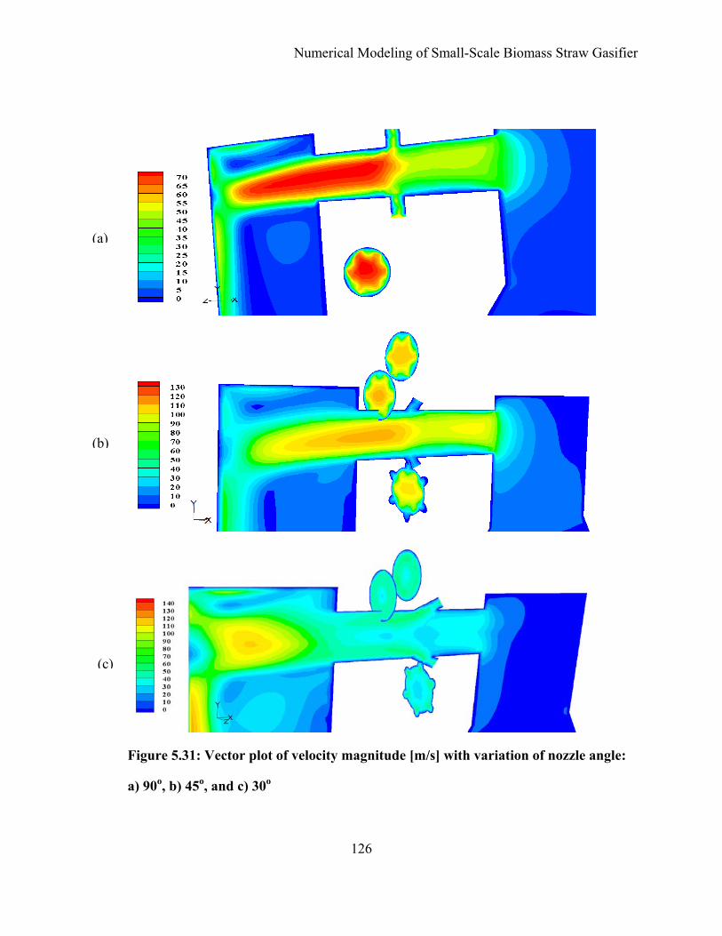
Numerical Modeling of Small-Scale Biomass Straw Gasifier
126
Figure 5.31: Vector plot of velocity magnitude [m/s] with variation of nozzle angle:
a) 90o, b) 45o, and c) 30o
(a)
(b)
(c)

Numerical Modeling of Small-Scale Biomass Straw Gasifier
127
Figure 5.32: Pathlines colored by ID with variation of secondary air nozzle angle: a) 90o, b) 45o and c) 30o
(a)
(b)
(c)

Numerical Modeling of Small-Scale Biomass Straw Gasifier
128
Figure 5.33: Vector plot of velocity magnitude [m/s] with variation of nozzle angle: a) 90o, b) 45o and c) 30o
(a)
(b)
(c)

Numerical Modeling of Small-Scale Biomass Straw Gasifier
129
Figure 5.34: Flow pattern tangential (a) versus perpendicular (b) to duct nozzle
5.6.3 Secondary to primary air ratio
The gasifier system under investigation relies on a negative draft pressure above the bed for
controls. The negative pressure in turn affects the hydrodynamics, heat transfer and reaction rates
during gasification processes. In addition, maintaining the system at below atmospheric pressure
avoids “blow back,” a potentially dangerous condition when flue gas is blown outside the
gasifier through view ports or the fuel feeder. Therefore, knowledge about the secondary to
primary air ratio that depends on primary air flow helped to make the adjustment that is required
to deliver sufficient air to maintain the desired straw bed height and maintain the lower primary
chamber region in a substoichiometric (insufficient air for complete combustion) environment.
To investigate the effect of primary air flow rate, the primary air flow rate was spanned from
0.16 kg/s to 0.35 kg/s (25%, 40% and 60% of the secondary air respectively) without preheat
(320 K) and with a moisture level of 14%. The pressure drop across the fuel bed for the three
secondary-to-primary ratios were compared, as shown in Figure 5.35. The pressure drop
increased with air flow increase. The contours of the velocity magnitude are shown in
Figure 5.36. The recirculation zones both at the exit from primary chamber and inlet to the
secondary chamber showed significant variation. The velocity contours also showed that the
velocity magnitude in the secondary mixer (see Section 5.3.2) increased as the primary air flow
rate increased.
The air flow rate influenced both the temperature profile and the distribution of gaseous
products. The mass fractions of the gases are compared for the three cases in Figure 5.37. The
(a) (b)

Numerical Modeling of Small-Scale Biomass Straw Gasifier
130
temperature contour plots using various flow rates of primary air (oxidation agent) are shown in
Figure 5.38. The higher the flow rate of air was introduced in the gasifier, the shorter the time
was required to reach high temperatures and maximum concentrations of the gaseous products.
At a fixed moisture level, the burning rate increased as the airflow rate increased until a critical
point is reached, beyond which a further increase in the air flow resulted in the fall of the burning
rate. The reason for this result is attributed to the fact that as the air flow increases beyond a
certain point, air channeling occurs. Relatively high temperature in the upper section of the
primary chamber and an unusually low temperature in the secondary chamber was observed
when the primary air flow rate is raised to 0.35 kg/s. The rapid consumption of biomass in
combustion at a high flow rate of air caused a fast decrease in the concentrations of gaseous
products. At lower flow rates of primary air, the time needed to heat up the reactor and to obtain
maximum concentrations of gaseous products is longer; the consumption of biomass was also
slower. The temperature on the top part of the secondary chamber was low when the primary air
flow was 0.16 kg/s. As a result, the favorable condition for the conversion of CO to CO2 is not
present when the primary air flow rate was set to 0.16 kg/s. The contour for mass fraction of O2
is also given on Figure 5.39. An increase of mass fraction of CO from less than 0.5% to 6.4%
showed the lack of conversion of CO to CO2. As a result, the temperature was low in at the top
part of the secondary chamber.
Figure 5.35: Effect of primary air flow on pressure drop

Numerical Modeling of Small-Scale Biomass Straw Gasifier
131
Figure 5.36: Contours of velocity magnitude [m/s] with variation in primary air: a) 0.16 kg/s, b) 0.24 kg/s and c) 0.35 kg/s
(a)
(b)
(c)

Numerical Modeling of Small-Scale Biomass Straw Gasifier
132
Figure 5.37: Effect of primary air flow rate on composition of gases at the secondary exit
Primary air flow rate [kg/s] O2 CO2 H2O CH4 H2 CO

Numerical Modeling of Small-Scale Biomass Straw Gasifier
133
Figure 5.38: Contours of temperature [K] with variation in primary air flow rate
(a)
(b)
(c)

Numerical Modeling of Small-Scale Biomass Straw Gasifier
134
Figure 5.39: Contours of mass fraction of O2 with variations in primary air flow rate: a) 0.16 kg/s, b) 0.25 kg/s and c) 35 kg/s
(a)
(b)
(c)

Numerical Modeling of Small-Scale Biomass Straw Gasifier
135
5.6.4 Straw bed height
The bed height is responsible for the variation of density and porosity. Therefore, its effect was
simulated to understand its impact on the gasification process. The fuel bed for the base case is
70% (ratio of 0.7) of the cylinder part of the primary chamber, 104.5 cm (for dimensions refer to
Appendix A). A fuel bed height of 0.8 and 0.6 times the primary cylinder is investigated with
bed heights of 119.4 cm and 89.5 cm, respectively (Figure 5.40). The effects on the composition
of the gases are shown in Figure 5.42. The variation in bed height resulted in the syngas yield
increase, particularly the mass fraction of H2, CO, CO2 and methane because for a given
temperature, higher fuel bed heights increase the time that the fuel will be available for reactions
to occur (residence time).
Figure 5.40: Bed height as ratio of primary chamber cylinder part
Height = 119.4 cm Height = 104.5 cm Height = 89.5 cm

Numerical Modeling of Small-Scale Biomass Straw Gasifier
136
Figure 5.41: Effect of bed height on mass composition of gases: a) 0.6, b) 0.7 and 0.8 times cylinder part of primary chamber
5.6.5 Variation of biomass
Different biomass fuels were investigated during gasification. The biomasses used for the study
in addition to straw were slough hay and wood chips because these are prevalent in the Prairies.
The inputs for the simulation were obtained based on the ultimate and proximate analyses of
different biomass fuels. The ultimate and proximate analyse for these biomasses are given on
Tables 5.7 and 5.8, respectively.

Numerical Modeling of Small-Scale Biomass Straw Gasifier
137
Table 5.7: Ultimate analysis for slough hay and wood chips
Sample Basis MC (%)
Ash (%)
VM (%) FC (%)
CV kJ/kg
Slough hay A.R. 31.56 5.23 51.70 11.51 12433
A.D. 4.03 7.33 72.50 16.14 17435 Dry ----- 7.64 75.54 16.82 18167
Wood Chips
A.R. 19.57 0.38 67.95 12.11 16309
A.D. 2.21 0.46 82.61 14.72 19829 Dry ----- 0.47 84.48 15.05 20277
Table 5.8: Proximate analysis results
Sample Basis MC (%)
C (%)
H (%)
Ash (%)
N (%)
O (%)
Slough hay A.R. 31.56 33.14 3.69 5.23 0.88 25.34 A.D. 4.03 46.48 5.17 7.33 1.23 35.54 Dry ----- 48.43 5.39 7.64 1.28 37.03
Wood chips
A.R. 19.57 42.70 4.91 0.38 0.49 31.94 A.D. 2.21 51.92 5.96 0.46 0.60 38.84 Dry ----- 53.09 6.10 0.47 0.61 39.71
It is worthy to note the variation of volatile matter, moisture content and calorific value of these
biomasses. Even though the other operating conditions were maintained the same as the
operating conditions used for wheat straw gasification, the composition of the fuel had a
significant effect on the outcome of the gasification process. It was also difficult to show a direct
comparison of the parameters in question since the effects of each are not linear.
The effect of biomass variation on gas composition is shown on Figure 5.43. The CO2 and H2O
mass fractions showed a significant decrease. The secondary temperature comparison is provided
in Figure 5.44. The temperature in the secondary chamber during the simulation of gasification
of wood chip is significantly higher than the one obtained for slough hay and wheat straw. The
contours plot for the three temperatures is shown in Figure 5.45. The reason for a higher
temperature for the wood chips is that at a fixed air flow rate, wood chips had a higher burning
rate and therefore had a higher flame temperature. The small diameter of wood chips also

Numerical Modeling of Small-Scale Biomass Straw Gasifier
138
favours the preheating and pyrolysis process and hence contributed to the high temperature in the
primary chamber (Figure 5.45). Figure 5.46 shows the contours of velocity magnitudes for the
three fuels and a slight drop in the velocity magnitude was observed.
Figure 5.42: Effect of biomass variation on composition of gases at secondary outlet
Figure 5.43: Effect of biomass type on outlet temperature in secondary chamber
O2 CO2 H2O CH4 H2 CO

Numerical Modeling of Small-Scale Biomass Straw Gasifier
139
Figure 5.44: Contours of temperature [K] with variation of biomass: a) wheat straw, b) slough hay and c) wood chip
(a)
(b)
(c)

Numerical Modeling of Small-Scale Biomass Straw Gasifier
140
Figure 5.45: Contours of velocity magnitude [m/s] with variation of biomass: a) wheat straw, b) slough hay, and c) wood chips
(a)
(b)
(c)

Numerical Modeling of Small-Scale Biomass Straw Gasifier
141
5.7 Impact on control strategy
The simulations above produced results of practical use for biomass gasification design. CFD
simulations were relatively simple to perform once the base case model had been formulated and
validated with experimental data and the equilibrium model. The results can be used for design
and optimization. These simulations can also be used for system scaling-up purposes. As for the
Vidir best gasifier, the CFD showed how the controller should react to changes in secondary-to-
primary air ratio and moisture content because these were found to be the most influencing factors
in the gasification processes.
It is necessary to have the correct air-to-fuel ratio to achieve complete gasification. With lower
values of this ratio an excess of charcoal and tar is produced, and with higher values charcoal is
depleted and product gas is burnt. Hence, it is crucial to have a means to get the optimum ratio for
an efficient and safe operation of the gasifier.
The air flow control system has a direct effect on the temperature. The gasifier system is
controlled by negative draft pressure above the bed. The negative pressure in turn affects the
hydrodynamics, heat transfer and reaction rates during gasification processes. In addition,
maintaining the system at below atmospheric pressure avoids “blow back” and maintains the
gasifier under negative pressure to prevent potential dangerous conditions, for unattended
operation. Therefore, control of the secondary-to-primary air ratio that depends on the primary air
flow helps to make the required adjustment to deliver sufficient air to maintain the desired pile
height and maintain the lower primary chamber region in a substoichiometric (insufficient air for
complete combustion) environment. Results from the simulation have shown that the pressure
drop across the fuel bed increases with air flow increase. As a result the variation in pressure drop
has influenced both the temperature profile and the distribution of gaseous products. Therefore,
having a means to control the secondary-to-primary ratio that amounts to having the necessary
oxygen enter the system plays a significance role in controlling the temperature and hence the
whole gasification process.
Oxygen monitoring, which is directly related to secondary-to-primary air ratio is the most
effective approach because it has a measurable single-value relationship with excess air, it is

Numerical Modeling of Small-Scale Biomass Straw Gasifier
142
insensitive to other flue gases, and it is independent of fuel composition. There are certain
precautions to observe. The sampling location must be carefully selected to minimize effects of
stratification and infiltration of damp air, which will falsely raise the O2 reading. To ensure safe
burner conditions, it is usually necessary to control flue gas oxygen to 8% or higher to ensure
complete combustion of fuel. When a shorter time is required to reach high temperatures and
maximum concentrations of the gaseous products, the air introduced in to the gasifier has to be
dialled up. At a fixed moisture level, the burning rate increases as the airflow rate increases until a
critical point is reached, beyond which a further increase in the air flow results in the fall of the
burning rate as a result of air channelling. When a biomass with low moisture content is used,
turning the air flow rate to low helps to increase the time needed to heat up the reactor and also
slows down the consumption of biomass. As a consequence, temperature in the gasifier can be
kept below the critical temperature to help reduce corrosion and air pollution by minimizing
formation of NOx.
Monitoring CO coming out of an exhaust stack can provide very close to stoichiometric
combustion by ensuring the absolute minimum of excess air. This is because CO is a direct
measure of combustion. The ideal CO level from the exhaust stack is near 200 ppm, (parts per
million) which is less than 0.02% CO. This low level requires relatively expensive sensing
techniques and computerized signal conditioning, which may only be justified on large boilers or
process heaters.
The results from the simulation indicated that fuels with high moisture content lower the reactor
temperatures due to the amount of energy needed to dry, vaporize and superheat the water, which
results in the production of lower energy syngas. The amount of required air increases when
moisture content increases to maintain the required reaction temperature. However, increasing the
amount of air randomly causes many disadvantages and one of which is the mass fraction
reduction of useful gases that consequently reduce the heating value. Use of preheated air
promotes drying of the fuel bed and also provides additional energy in the pre-destruction stage,
which enhances the thermal decomposition characteristics of the biomass, thus higher calorific
value syngas is produced.

Numerical Modeling of Small-Scale Biomass Straw Gasifier
143
Combustible gases released from the solid fuel have to mix first with the secondary air before their
combustion can take place, i.e. the burning of the gases fuel is limited not only by the reaction
kinetics but also by the mixing rate of producer gases with the secondary air. A simple, adjustable
nozzle to optimize the flow pattern of the jet mixing into the bulk gas based on secondary
temperature can be implemented that, in turn, can be controlled by the air flow.

Numerical Modeling of Small-Scale Biomass Straw Gasifier
144
Chapter 6. Conclusion and recommendations
6.1 Conclusion
The use of agricultural residues as feedstock for gasification process has been presented.
FLUENT® was used for comprehensive simulations of the four different stages of gasification
processes namely drying, pyrolysis, gasification and combustion taking place inside a 900-kWth
two-stage gasifier. Compositions of combustible gases released from straw, slough hay and
wood chips gasification were predicted. The model was divided into transport and chemistry
equations. The equations were numerically solved simultaneously to yield the solution for the
profiles of gas composition and temperature along the gasifier chambers. The results were then
compared with experimental data to show the accuracy of the model. The effects of feedstock on
this process were explained. It was found that the major physical properties affecting this process
are size, shape, size distribution and density of feedstock. Size, form, and size distributions of
feedstock mainly affect the porosity and hence the pressure-drop across the gasifier chamber bed.
It was observed that in order to deliver sufficient air to maintain the desired bed height and
maintain the lower primary chamber region in a substoichiometric (insufficient air for complete
combustion) environment, between 40% and 60% of the required air must be supplied. Thermo-
chemical properties, heating value, chemical composition, moisture content, volatile matter and
ash content influenced the producer gas production. The moisture content of biomass had a great
impact on its effectiveness as a fuel source since considerable energy was consumed (2,444
kJ/kg) to evaporate this water without doing any useful work in the process. High moisture
content decreased calorific value impacting operations. Operating parameters of the gasifier such
as temperature, air-to-mass ratio, and primary-to-secondary ratio were also found critical to the
composition of gases and the rate of gasification.
Ash composition of the biomass materials is crucial to agglomeration problems which ultimately
results in fouling of the gasifier. Depending on the ash composition and the local bed
temperatures, a degree of sintering or fusion of the bed ash may occur. This is often exacerbated
by imperfect fuel distribution over the grate. If the degree of fusion of the ash is excessive,
relatively large ash agglomerates may form, and this can interfere with the distribution of the

Numerical Modeling of Small-Scale Biomass Straw Gasifier
145
combustion air through the fuel bed and affects burnout of the char and the quality of the gaseous
and gas-borne emission levels.
The temperature profiles of the producer gas and inside the chambers provided an understanding
of the phenomena taking place for the gasification process. It was shown that the temperature
levels in the gasifier affected the gas composition and the calorific value of the producer gas.
Increasing the air velocity, while maintaining a specified amount of biomass fed into the reactor
results in a higher burning rate as the oxygen penetrates farther into the bed. This consumes char
at a greater rate, increasing the overall temperature of the bed, which increases the rate of heat
transfer to the fuel. This in turn increases the drying and pyrolysis and gasification rate of the
fuel. The optimisation of the gasification process can result in higher carbon conversion rates,
and a corresponding reduction in the total particulate levels and the carbon content of the
particulates. Consequently, the knowledge of the temperature profiles, which is directly related
to the amount of air delivered to the system, is necessary for optimizing the performance of the
gasifier.
6.2 Recommendations
The simulated results provided a realistic impression of the gasification process, and enabled the
discussion of controlling parameters in this complex physical and reaction behaviour in a two-
stage gasifier for a better operation of the gasifier, which depends on an optimum air control
system. The following recommendations are put forward for consideration:
• Preheating of the primary air would increase the flame propagation speed by minimizing the
convective heat loss from the drying or burning fuel particles.
• Since the knowledge of the temperature is directly related to the amount of air delivered to
the system it is necessary to optimize the performance of the gasifier. When burning dry fuel
it would be helpful to equip the system with a fuel conditioning system: water spray.
Inserting a thermocouple into the neck of the primary chamber with its output going to the
PLC would actuate the fuel conditioning system. When the chamber temperature is reached
to an operator-set temperature, it can activate the system opening a solenoid. This simple
function does not actually increase the moisture content of the fuel, but rather it coats the fuel

Numerical Modeling of Small-Scale Biomass Straw Gasifier
146
with just enough water to slow the gasification process and reduce the gasifier temperature to
acceptable levels.
• The combustion system relies on a negative draft pressure. Given that the under grate air
supply follows the fuel, both are controlled through the PLC and act linearly. Therefore,
there has to be a means to control the fuel bed and the pressure separately so that the fan is
not only reacting to pressure changes but rather to gasification process changes: as more fuel
is required and delivered, the oxygen level would decrease causing the fan’s variable
frequency drive to increase the fan speed thus increasing the primary airflow.
• A gas analyzer probe at the exit of primary chamber is recommended. An analyzer
specialized for the purpose of measuring the components in flue gas and calculating the
relevant results from the temperature and gas readings would help to make adjustments on
the gasifier system and the effects could be seen immediately. The readings from the
analyzer would also help improve the validation of the CFD model in a more accurate way.

Numerical Modeling of Small-Scale Biomass Straw Gasifier
147
References
[1]. Babu, S.P. & Whaley, T.P. (1992). IEA Biomass Thermal Gasification Project, Biomass
and Bioenergy, Vol. 2, No. 1-6, pp. 299-306.
[2]. Maniatis, K. (2000). Progress in Biomass Gasification: an Overview, Progress in
Thermochemical Biomass Conversion, Tyrol, Austria, 17-22 September 2000, Vol. 1, pp.
1-31.
[3]. Knudsen, J.N. et al. (2001). Experimental Investigation of Sulfur Release During
Thermal Conversion of Wheat Straw and its Application to Full-scale Grate Firing, Sixth
International Conference on Technologies and Combustion for a Clean Environment, 9-
12 July, 2001, Oporto (Portugal), Vol. 3, pp. 1303-1309.
[4]. Brown, D. P., Biswas, P. and Rubon, S. G. (1994). Transport and Deposition of Particles
in Gas Turbine; Effects of Convection; Diffusion, Thermophoresis, Inertial Impaction
and Cogeneration, FACT-Vol. 18, Combustion Modeling, Scaling and Air Toxins,
ASME, pp. 69-76.
[5]. Bridgwater, A.V. (1995). The Technical and Economic Feasibility of Biomass
Gasification for Power Generation, Fuel, Vol. 74, No. 5, pp. 631-653.
[6]. Booth, R. & Elliott, P. (1993). Biomass Energy Overview, European Seminar
BIOWATT, Innovative Technologies for the Production of Electricity from Biomass,
October 4-5, Milan, Italy. (Preprints)
[7]. Di Blasi, C., Signorelli, G. & Portoricco, G. (1999). Countercurrent Fixed-Bed
Gasification of Biomass at Laboratory Scale, Industrial & Engineering Chemistry
Research, Vol. 38, pp. 2571-2581.
[8]. Fercher, E., Hofbauer, H., Fleck, T., Rauch, R. & Veronik, G. (1998). Two Years
Experience with the FICFB-Gasification process, Biomass for Energy and Industry. 10th
European Conference and Technology Exhibition, 8-11 June 1998, Würzburg, Germany,
pp. 280-283.
[9]. Evans, R.J. & Milne, T.A. (1997). Chemistry of Tar Formation and Maturation in the
Thermochemical Conversion of Biomass, Developments in Thermochemical Biomass
Conversion, Blackie Academic & Professional, 1997, pp. 803-816.

Numerical Modeling of Small-Scale Biomass Straw Gasifier
148
[10]. Easterly, J.L. & Burnham, M. (1996). Overview of Biomass and Waste Fuel Resources
for Power Production, Biomass and Bioenergy, Vol. 10, No. 2-3, pp. 79- 92.
[11]. Dixon, T. F., Mann, A. P., Plaza, F., Gilfillan, W. N. (2005). Development of Advanced
Technology for Biomass Combustion – CFD as an Essential Tool. Fuel, Vol. 84, No. 10,
pp. 1303-1311.
[12]. Miltner, M., Miltner, A.; Harasek, M., Friedl, A. (2007). Process Simulation and CFD
Calculations for the Development of an Innovative Baled Biomass-fired Combustion
Chamber. Applied Thermal Engineering, Vol. 27, No. 7, pp.1138-1143.
[13]. Platiau, D. & Faniel, Y. (1989). The AVSA Biomass Gasification Process, Energy from
Biomass 4. Proceedings of the 3rd contractors' meeting, Paestum, 25- 27 May 1988, pp.
563-579.
[14]. Reed, T.B. & Das, A. (1988). Handbook of Biomass Downdraft Gasifier Engine Systems.
The Biomass Energy Foundation Press, 1810 Smith Rd., Golden, CO.
[15]. Abatzoglou, N. et al. (2000). The Development of a Draft Protocol for the Sampling and
Analysis of Particulate and Organic Contaminants in the Gas from Small Biomass
Gasifiers, Biomass and Bioenergy, Vol 18, pp. 5-17.
[16]. D'Apote, S.L. (1998). IEA Biomass Energy Analysis and Projections, Biomass Energy:
Data, Analysis and Trends, Conference proceedings, Paris, France, 23-24 March 1998,
IEA.
[17]. Kandaswamy, D.S., Warren, D.W. & Mansour, M.N. (1991). Indirect Steam Gasification
of Paper mill Sludge waste, Tappi Journal, Vol. 74, No. 10, pp. 137- 143.
[18]. Marklund M.; Tegman R.; Gebart R. (2007). CFD Modeling of Black Liquor
Gasification: Identification of important Model Parameters. Fuel, 86, pp.1918-1926.
[19]. Environment Canada. (1993). Reference Methods for Source Testing: Measurement of
Releases of Particulate from Stationary Sources. Reference Method EPS 1/RM/8.
[20]. Esubeo C, (1999). Biomass Conversion Technologies, Achievements and Prospects for
Heat and Power Generation, report EUR 18029, pp. 94-95.
[21]. Campbell, C.A. et al. (2002). Production of annual crops on the Canadian Prairies:
Trends during 1976–1998. Canadian Journal of Soil Science, Vol. 82, pp. 45-57.

Numerical Modeling of Small-Scale Biomass Straw Gasifier
149
[22]. Sokhansanj S. et al. (2006). Production and distribution of cereal straw on the Canadian
prairies. Canadian Biosystems Engineering, Vol. 48, pp. 9-11.
[23]. Manitoba Agriculture Yearbook. (2003). http://www.gov.mb.ca/
agriculture/statistics/aac16s00.html (2007/09/25).
[24]. Aznar, M.P., Corella, J., Delgado, J. & Lahoz, J. (1993). Improved Steam Gasification of
Lignocellulosic Residues in a Fluidized Bed with Commercial Steam Reforming
Catalysts, Industrial & Engineering Chemistry Research, Vol. 32, pp. 1-10.
[25]. Leverage, Graham. (2008). Summer Internship. University of Manitoba.
[26]. Cen, K. et al. (1993). Research on Rice Hulls Gasification Gas/Steam Co-generation
System Using a Circulating Fluidized Bed, ENERGEX '93 - The 5th International Energy
Conference, 18-22 October, 1993. Vol. 3, pp. 683-692.
[27]. Fletcher, D. F.; Haynes, B. S.; Christo, F. C.; Joseph, S. D. (2000). A CFD Based
Combustion Model of an Entrained Flow Biomass Gasifier. Applied Mathematical
Modeling, Vol. 24, No. 3, pp. 165-182.
[28]. Hallgren, A. (1996). Theoretical and Engineering Aspects of the Gasification of Biomass,
Ph.D. Thesis, Lund University, Sweden.
[29]. Hulkkonen, S., Äijlälä, M. & Holappa, J, (1993). Integration of a Fuel Dryer to a Gas
Turbine Process, ASME Cogen Turbo Power '93. IGTI, Vol. 8, pp. 61-67.
[30]. Kær, S. K. (2004). Numerical Modeling of a Straw-fired Grate Boiler. Fuel, Vol. 83,
No.9, pp.1183-1190.
[31]. Hoppesteyn, P.D.J., De Jong, W., Andries, J. & Hein, K.R.G. (1997). Combustion of
Biomass-derived Low Calorific Value Gas, Combustion and Emissions Control III, The
Institute of Energy, Pergamon, London.
[32]. Antal, M.J. (1982). Biomass Pyrolysis: A Review of the Literature. Part 1 – Carbohydrate
Pyrolysis, Advances in Solar Energy, Vol. 1, pp. 61-111.
[33]. Kær, S. K.; Rosendahl, L. A.; Baxter, L. L. (2004). Extending the Capability of CFD
Codes to Assess Ash Related Problems in Biomass Fired Boilers. In Proc. 227th ACS
Annual Meeting¸ Anaheim California, Mar 28-Apr 1, 2004; Division of Fuel Chemistry,
No. 12.

Numerical Modeling of Small-Scale Biomass Straw Gasifier
150
[34]. Blasi, C. D. (2008). Modeling Chemical and Physical Processes of Wood and Biomass
Pyrolysis. Progress in Energy and Combustion Science, Vol. 34, pp. 47-90.
[35]. Magnussen, B. F. Hjertager, B. H. (1976). On Mathematical Modeling of Turbulent
Combustion with Special Emphasis on Soot Formation and Combustion. In: Proc. 16th
Symp. (Int.) on Combustion, the Combustion Institute (Ed.), Pittsburgh, USA, pp. 719-
729.
[36]. Roos, A. et al. (1999). Critical Factors to Bioenergy Implementation, Biomass and
Bioenergy, Vol. 17, pp. 113-126.
[37]. Aldén, H., Hagström, P., Hallgren, A. & Waldheim, L. (1997). Investigations in High
Temperature Catalytic Gas Cleaning for Pressurized Gasification Processes,
Developments in Thermochemical Biomass Conversion, Blackie Academic &
Professional, pp. 1131-1143.
[38]. Fredriksson, C. & Kjellström, B. (1997). Alkali Separator in Steam Injected Cyclone
Wood Powder Gasifier for Gas Turbine Application, Developments in Thermochemical
Biomass Conversion, Blackie Academic & Professional, pp. 921-931.
[39]. Rapagnà, S. & Foscolo, P.U. (1996). Gasification of Biomass in a Fluidised Bed Reactor:
The Influence of Temperature and Biomass Particle Size, Biomass for Energy and the
Environment. Proceedings of the 9th European Bioenergy Conference, June 1996,
Copenhagen, Denmark.
[40]. Launder, B. E. and Spalding, D. B. (1974), The Numerical Computation of Turbulent
Flows, Computer Methods in Applied Mechanics and Engineering, Vol. 3, pp. 269-289.
[41]. Holt, N.A. & van der Burgt, M.J. (1998). Biomass Conversion: Prospects and Context,
Power Production from Biomass III, Gasification and Pyrolysis R&D&D for Industry,
14-15 September, Espoo, Finland, pp. 163-177.
[42]. Herguido, J., Corella, J., Artal, G. & Garcia-Bordeje, J.E. (1992). Results with a
Multisolid Circulating Fluid Bed Pilot Plant for the Improved Steam Gasification of
Biomass, Biomass for Energy, Industry and the Environment, pp. 792-796.
[43]. Neeft, J.P.A. et al. (2000). Guideline for Sampling and Analysis of "tars" and Particles in
Biomass Producer Gases, Progress in Thermochemical Biomass Conversion, Tyrol,
Austria, 17-22 September 2000.

Numerical Modeling of Small-Scale Biomass Straw Gasifier
151
[44]. Sommerfeld, M. (2002). Numerical Method for Calculating Particle Dispersion in
Turbulent Flow, Sixth Workshop on Two-Phase Flow Predictions, Erlangen, March 30 –
April 2, 2002.
[45]. Beck, S.R. Wang, M.J. & Hightower, J.A. (1981). Gasification of Oak Sawdust,
Mesquite, Corn Stover and Cotton Gin Trash in a Countercurrent Fluidized Bed Pilot
Reactor, Biomass as a Non-fossil Fuel Source, ACS Symposium Series 144, pp. 335-349.
[46]. Bentzen, J.D., Henriksen, U. & Hansen, C.H. (1999). Investigations of a Two-stage
gasifier, 2nd Olle Lindström Symposium on Renewable Energy, Royal Institute of
Technology, Stockholm, Sweden, June 1999, pp. 117-120.
[47]. Christensen K. A. (1995). The Formation of Submicron Particles from the Combustion of
Straw, Ph.D. Thesis, ISBN 87-90142-04-7, Department of Chemical Engineering,
Technical University of Denmark, Lyngby, Denmark.
[48]. Sharma, A. K. (2007). Modeling fluid and Heat Transport in the Reactive, Porous Bed of
Downdraft (biomass) Gasifier. International Journal of Heat and Fluid Flow, Vol. 28, pp.
1518-1530.
[49]. Moilanen, A. & Saviharju, K. (1997). Gasification Reactivates of Biomass Fuels in
Pressurised Conditions and Product Gas Mixtures, Developments in Thermochemical
Biomass Conversion, Blackie Academic & Professional, pp. 828-837.
[50]. Saffman, P. G. (1965). The Lift on a Small Sphere in a Slow Shear Flow, Journal of Fluid
Mechanics, Vol. 22, Part 2, pp. 385-400.
[51]. Patankar S.V. (1980). Numerical Heat Transfer and Fluid Flow. Hemisphere,
Washington, D.C.
[52]. Ahrenfeldt, J., Henriksen, U. & Schramm, J. (2000). Experimental on Wood Gas
Engines, The Technical University of Denmark, Department of Energy Engineering, ET-
ES 2000-04.
[53]. Habibi, A., Merci, B., Heynderickx, G. J. (2007). Impact of Radiation Models in CFD
Simulations of Steam Cracking Furnaces. Computers & Chemical Engineering, Vol. 31,
No. 11, pp. 1389-1406.

Numerical Modeling of Small-Scale Biomass Straw Gasifier
152
[54]. Zhou, H., Jensen, P.A., Flemming, J.F. (2007). Dynamic Mechanistic Model of
Superheater Deposit Growth and Shedding in a Biomass Fired Grate Boiler. Fuel, Vol. 86
pp. 1519-1533.
[55]. Bentzen, J.D. & Henriksen, U. (2000). Condensate from a Two-stage Gasifier, 1st World
Conference on Biomass for Energy and Industry, Sevilla, Spain, 5-9 June 2000.
[56]. Babu, B.V. and Sheth, P.N. (2005). Modeling and Simulation of Reduction Zone of
Downdraft Biomass Gasifier: Effect of Char Reactivity Factor, Communicated to Energy
Conversion and Management.
[57]. Baxter L.L. (2005). Towards a CFD-based Mechanistic Deposit Formation Model for
Straw-fired Boilers. Fuel. Vol. 84, pp. 833-848.
[58]. Svendsgaard, O.B. (2000). Gas Engine for a Biomass Powered Small Scale Heat and
Power Plant, Diploma Report, Institute of Thermal Energy and HydroPower, Norwegian
University of Science and Technology (NTNU), Norway.
[59]. Xiu S. N., Wang N. N., Yi W.M.; Li B. M.; Shahbazi G. (2008). Validation of Kinetic
Parameter Values for Prediction of Pyrolysis Behaviour of Corn Stalks in a Horizontal
Entrained-flow Reactor. Biosystems Engineering, Vol. 100, pp. 79-85.
[60]. Brunner T., Joller M., Obernberger I. (2004). Aerosol Formation in Fixed-Bed Biomass
Furnaces: Results from Measurements and Modeling. Proc. of the Internat. Conf. Science
in Thermal and Chemical Biomass Conversion, Sept 2004, Victoria, Canada.
[61]. Xia, B.; Sun, D. W. (2002). Applications of Computational Fluid Dynamics (CFD) in the
Food Industry: a review. Computers and Electronics in Agriculture, Vol. 34, No. 1-3, pp.
5-24.
[62]. Bilbao, R., García, L., Salvador, M.L. & Arauzo, J. (1998). Steam Gasification of
Biomass in a Fluidized Bed, Effect of a Ni-Al catalyst, Biomass for Energy and Industry.
10th European Conference and Technology Exhibition, 8-11 June 1998, Würzburg,
Germany, pp. 1708-1711.
[63]. Gebhard, S.C., Wang, D., Overend, R.P. & Paisley, M.A. (1994). Catalytic Conditioning
of Synthesis Gas Produced by Biomass Gasification, Biomass and Bioenergy, Vol. 7, No.
1-6, pp. 307-313.

Numerical Modeling of Small-Scale Biomass Straw Gasifier
153
[64]. Brandt, P. & Henriksen, U. (1998). Decomposition of Tar in Pyrolysis Gas by Partial
Oxidation and Thermal Cracking. Part 2, Biomass for Energy and Industry. 10th
European Conference and Technology Exhibition, 8-11 June 1998, Würzburg, Germany.
[65]. Babu, B. V., Chaurasia, A. S. (2004). Pyrolysis of Biomass: Improved Models for
Simultaneous Kinetics and Transport of Heat, Mass and Momentum. Energy Conversion
and Management, Vol. 45, No. 9-10, pp. 1297-1327.
[66]. Larson, E.D. & Williams, R.H. (1988). Biomass-fired Steam-injected Gas Turbine
Cogeneration, ASME Cogen-Turbo II Proceedings, pp. 57-66.
[67]. Nordin, A., Kallner, P. & Johansson, E. (1997). Gas Quality from Biomass Gasification;
an Extensive Parametric Equilibrium Study, Developments in Thermochemical Biomass
Conversion, Blackie Academic & Professional, pp. 838-850.
[68]. Williams, R.H. & Larson, E.D. (1996). Biomass Gasifier Gas Turbine Power Generating
Technology, Biomass and Bioenergy, Vol. 10, No. 2-3, pp. 149-166.
[69]. Chughtai, M.Y. & Kubiak, H. (1998). Hydrogen from Biomass, Biomass for Energy and
Industry. 10th European Conference and Technology Exhibition, 8-11 June 1998,
Würzburg, Germany, pp. 284-286.
[70]. Fredriksson, C. & Kjellström, B. (1996). Cyclone Gasification of Steam Injected Wood
Powder, Nordic Seminar on Thermochemical Conversion of Solid Fuels, 4-6 December
1996, NTH, Trondheim, Norway.
[71]. Schlichting, H. and Gersten, K. (2000). Boundary Layer Theory, 8th Edition, Springer.
[72]. Higman C, van der Burgt M. Gasification. (2003). Gulf Professional Pub., USA.
[73]. Olivares, A., Aznar, M.P., Caballero, M.A., Gil, J., Francés, E. & Corella, J. (1997).
Biomass Gasification: Produced Gas Upgrading by In-bed Use of Dolomite, Industrial &
Engineering Chemistry Research, Vol. 36, pp. 5220-5226.
[74]. Rapagnà, S., Jand, N. & Foscolo, P.U. (1998). Utilisation of Suitable Catalysts for the
Gasification of Biomasses, Biomass for Energy and Industry. 10th European Conference
and Technology Exhibition, 8-11 June 1998, Würzburg, Germany, pp. 1720-1723.
[75]. Minowa, T., Ogi, T. & Yokoyama, S. (1997). Hydrogen Production from Lignocellulosic
Materials by Steam Gasification using a Reduced Nickel Catalyst, Developments in
Thermochemical Biomass Conversion, Blackie Academic & Professional, pp. 932-941.

Numerical Modeling of Small-Scale Biomass Straw Gasifier
154
[76]. Reed, T.B. & Das, A. (1988). Handbook of Biomass Downdraft Gasifier Engine Systems,
The Biomass Energy Foundation Press, 1810 Smith Rd., Golden, CO.
[77]. Janarthanan, A.K. & Clements, L.D. (1997). Gasification of Wood in a Pilot Scale
Spouted Bed Gasifier, Developments in Thermochemical Biomass Conversion, Blackie
Academic & Professional, pp. 945-959.
[78]. Grønli, M. (1996). Theoretical and Experimental Study of the Thermal Degradation of
Biomass, Ph. D. Thesis, Norwegian University of Science and Technology.
[79]. Kær, S. K., Rosendahl, L. (2003). Extending the Modeling Capacity of CFD Codes
Applied to Biomass-Fired Boilers. In Proc. ECOS, Copenhangen, Denmark, Jun 30-Jul 2,
2003, pp. 251-264.
[80]. Barbucci, P. & Trebbi, G. (1994). Biomass Based Systems for the Generation or
Cogeneration of Electricity, International Journal of Solar Energy, Vol. 15, pp. 171-178.
[81]. Willcox, D (1998). Turbulence Modeling for CFD. DCW Industries, California.
[82]. Mathieu, P. and Dubuisson, R. (2002). Performance Analysis of a Biomass gasifier,
Energy Conversion and Management, Vol. 43, No. 10, pp. 1291-1299.
[83]. Kandaswamy, D.S., Warren, D.W. & Mansour, M.N. (1991). Indirect Steam Gasification
of Paper mill Sludge waste, Tappi Journal, Vol. 74, No. 10, pp. 137- 143.
[84]. Milligan, J.B. (1994). Downdraft gasification of biomass. Ph.D. Thesis. Aston
University, Birmingham, UK.
[85]. Neilson, C.E. (1998). LM2500 Gas Turbine Modifications for Biomass Fuel Operation,
Biomass and Bioenergy, Vol. 15, No. 3, pp. 269-273.
[86]. Svendsgaard, O.B. (2000). Gas Engine for a Biomass Powered Small Scale Heatand
Power Plant, Diploma Report, Institute of Thermal Energy and HydroPower, Norwegian
University of Science and Technology (NTNU), Norway.
[87]. Vidir GDS. [Online]. Retrieved Jan. 1, 2009. Available at:
www.vidir.biz/vidirbiomass/vidirbiomass.ppt.htm .
[88]. Gil, J., Aznar, M.P., Caballero, M.A., Francés, E. & Corella, J. (1997). Biomass
Gasification in Fluidized Bed at Pilot Scale with Steam-oxygen Mixtures. Product
Distribution for Different Operating Conditions, Energy and Fuels, Vol. 11, pp. 1109-
1118.

Numerical Modeling of Small-Scale Biomass Straw Gasifier
155
[89]. Herguido, J., Corella, J. & González-Saiz, J. (1992). Steam Gasification of
Lignocellulosic Residues in a Fluidized Bed at a Small Pilot Scale. Effect of the Type of
Feedstock, Industrial & Engineering Chemistry Research, Vol. 31, pp. 1274-1282.
[90]. Yang Y. B., Sharifi V. N. (2007). Swithenbank J. Converting Moving-grate Incineration
from Combustion to Gasification - Numerical Simulation of the Burning Characteristics.
Waste Management, Vol. 27, pp. 645-655.
[91]. Zainal, Z.A., Ali, R., Lean, C.H. and Seetharamu, K. N. (2001). Prediction of
Performance of a Downdraft Gasifier Using Equilibrium Modeling for Different Biomass
Materials, Energy Conversion and Management, Vol. 42, No. 12, pp. 1499-1515.
[92]. Giltrap D.L., McKibbin, R. and Barnes, G.R.G. (2003). A Steady State Model of Gas-
char Reactions in a Down Draft Biomass Gasifier, Solar Energy, Vol. 74, No. 1, pp. 85-
91.
[93]. Kær, S. K., Rosendahl, L. A., Baxter, L. L. (2006). Towards a CFD-based Mechanistic
Deposit formation Model for Straw-fired Boilers. Fuel, Vol. 85, No. 5-6, pp. 833-848.
[94]. Maughan, J.R., Bowen, J.H., Cooke, D.H. & Tuzson, J.J. (1994). Reducing Gas Turbine
Emissions Through Hydrogen-enhanced, Steam-injected Combustion, ASME Cogen
Turbo Power '94. IGTI, Vol. 9, pp. 381-390.
[95]. Gerun L., Paraschiv M., Vijeu R., Bellettre J., Tazerout M., Gøbel B., Henriksen U.
(2008). Numerical Investigation of the Partial Oxidation in a Two-stage Downdraft
Gasifier. Fuel, Vol. 87, pp. 1383-1393.
[96]. Ma, L., Jones, J. M., Pourkashanian, M., Williams, A. (2007). Modeling the Combustion
of Pulverized Biomass in an Industrial Combustion Test Furnace. Fuel, Vol. 86, No. 12-
13, pp. 1959-1965.
[97]. Lammers, G., Beenackers, A.A.C.M. & Corella, J. (1997). Catalytic Tar Removal from
Biomass Producer Gas with Secondary Air, Developments in Thermochemical Biomass
Conversion, Blackie Academic & Professional, pp. 1179-1193.
[98]. Kallio, G. A. and Reeks, M. W. (1989). A Numerical Simulation of Particle Deposition in
Turbulent Boundary Layers, International Journal of Multiphase Flow, Vol. 15, No. 3,
pp. 433-446.

Numerical Modeling of Small-Scale Biomass Straw Gasifier
156
[99]. Luo, Z. Y., Wang, S. R., Cen, K. F. (2005). A Model of Wood Flash Pyrolysis in
Fluidized Bed Reactor. Renewable Energy, Vol. 30, No. 3, pp. 377-392.
[100]. Langner, J. (2007). Numerical Modeling of a Biomass Gasifier. MITACS-Vidir
Internship Report, University of Manitoba.
[101]. Syred, N., Kurniawan, K., Grifths, T., Gralton, T., Ray, R. (2007). Development of
Fragmentation Models for Solid Fuel Combustion and Gasification as Subroutines for
Inclusion in CFD Codes. Fuel, Vol. 86, No. 14, pp. 2221-2231.
[102]. Paisley, M.A. (1997). Catalytic Hot Gas Conditioning of Biomass derived Product gas,
Developments in Thermochemical Biomass Conversion, Blackie Academic &
Professional, 1997, pp. 1209-1223.
[103]. Ounis, H., Ahmadi, G. and Mclaughlin, J.B. (1991). Dispersion and Deposition of
Brownian Particles from Point Sources in a Simulated Turbulent Channel Flow,
Journal of Colloid and Interface Science, Vol. 147, No.1, pp. 233-250.
[104]. Dixon, T. F., Mann, A. P., Plaza, F. and Gilfillan, W. N. (2005). Development of
Advanced Technology for Biomass Combustion – CFD as an Essential Tool. Fuel,
Vol. 84, No. 10, pp. 1303-1311.
[105]. Pallares, J., Arauzo, I. and Williams, A. (2007). Integration of CFD Codes and
Advanced Combustion Models for Quantitative Burnout Determination. Fuel, Vol. 86,
pp. 2283-2290.
[106]. Crowe, C., Sommerfeld, M. and Tsuji, Y. (1997), Multiphase Flows with Droplets and
Particles, CRC Press.
[107]. Rapagnà, S., Jand, N. & Foscolo, P.U. (1998). Catalytic Gasification of Biomass to
Produce Hydrogen Rich Gas, International Journal of Hydrogen Energy, Vol. 23, No.
7, pp. 551-557.
[108]. Shanmukharadhya, K. S., Sudhakar, K. G. (2007). Effect of Fuel Moisture on
Combustion in a Bagasse Fired Furnace. Journal of Energy Resources Technology-
Transactions of the ASME, Vol. 129, No. 3, pp. 248-253.
[109]. Fluent 6.2. (2003). User's Guide. Fluent Incorporated.
[110]. Zarnescu, V., Pisupati, S. V. (2002). An Integrative Approach for Combustor Design
Using CFD Methods. Energy & Fuels, Vol. 16, No. 3, pp. 622-633.

Numerical Modeling of Small-Scale Biomass Straw Gasifier
157
[111]. Obernberger I., Brunner T., Joller M. (2001). Characterisation and Formation of
Aerosols and Fly-Ashes from Fixed-Bed Biomass Combustion. In: Proceedings of the
international IEA Seminar “Aerosols in Biomass Combustion,” Zuerich, Switzerland,
ISBN 3-908705-00-2, pp. 69-74.
[112]. Oser M., Nussbaumer T., Muller P., Mohr M., Figi R. (2004). Mechanisms of Particle
Formation in Biomass Combustion. In: Proceedings of the Second World Biomass
Conference, 10-14 May 2004, ISBN 88-89407-04-2, pp. 1246-1249.

Numerical Modeling of Small-Scale Biomass Straw Gasifier
158
Appendix A. Gasifier dimensions and FLUENT® model set up
Figure A.1: Dimensions of 900-kWth Vidir proprietary gasifier modelled

Numerical Modeling of Small-Scale Biomass Straw Gasifier
159
Table A.1: Solid straw and combusting straw particles properties
Straw Units
Material type solid
Density 410 kg/m3
Cp 1250 J/kg K
Thermal conductivity 0.05 W/m K
Straw-particles Units
Material type combusting-particle
Density 410 kg/m3
Cp 1250 J/kg K
Thermal conductivity 0.05 W/m K
Vaporization temperature 400 kg/m3
Volatile comp. fraction 79.28 %
Binary diffusivity 4.00E-05 m2/s
Swelling coefficient 1
Burnout stoichiometric ratio 1.333
Combustible fraction 16.03 %
Heat of rxn for burnout 9202211 J/kg
Devolatilization model single rate 1/s
Combustion model diffusion-limited

Numerical Modeling of Small-Scale Biomass Straw Gasifier
160
Table A.2: Straw-volatiles and straw-vol-air properties
Straw-volatiles Units
Material type fluid
Mixture straw-volatiles-air
Cp 1500 J/kg K
Molecular weight 32.83027 kg/kmol
Standard state enthalpy -32443550 J/kmol
Standard state entropy 0 J/kmol
Reference temperature 298.15 K
Straw-volatiles-air Units
Material type mixture
Density incompressible-ideal-gas
Cp mixing law J/kg K
Thermal conductivity 0.0454 W/m K
Viscosity 1.72E-05 kg/m. s
Mass diffusivity 2.88E-05 m2/s
Absorption coefficient 0 1/m
Scattering coefficient 0 1/m
Scattering phase function isotropic

Numerical Modeling of Small-Scale Biomass Straw Gasifier
161
Table A.3: CH4 and CO properties
CH4 Units
Material type fluid
Mixture straw-volatiles-air
Cp piecewise-polynomial J/kg K
Molecular weight 16.04276 kg/kmol
Standard state enthalpy -7.49E+07 J/kmol
Standard state entropy 186043.9 J/kmol
Reference temperature 298 K
CO Units
Material type fluid
Mixture straw-volatiles-air
Cp piecewise-polynomial J/kg K
Molecular weight 28.0104 kg/kmol
Standard state enthalpy -1.11E+08 J/kmol
Standard state entropy 197535.7 J/kmol
Reference temperature 298 K
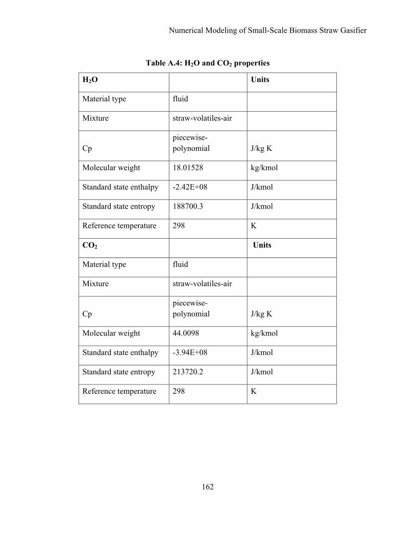
Numerical Modeling of Small-Scale Biomass Straw Gasifier
162
Table A.4: H2O and CO2 properties
H2O Units
Material type fluid
Mixture straw-volatiles-air
Cp piecewise-polynomial J/kg K
Molecular weight 18.01528 kg/kmol
Standard state enthalpy -2.42E+08 J/kmol
Standard state entropy 188700.3 J/kmol
Reference temperature 298 K
CO2 Units
Material type fluid
Mixture straw-volatiles-air
Cp piecewise-polynomial J/kg K
Molecular weight 44.0098 kg/kmol
Standard state enthalpy -3.94E+08 J/kmol
Standard state entropy 213720.2 J/kmol
Reference temperature 298 K

Numerical Modeling of Small-Scale Biomass Straw Gasifier
163
Table A.5: H2, N2 and O2 properties
H2 Units Material type fluid Mixture straw-volatiles-air Cp piecewise-polynomial J/kg K Molecular weight 2.01588 kg/kmol Standard state enthalpy -1882.081 J/kmol Standard state entropy 130581.7 J/kmol Reference temperature 298 K N2 Units Material type fluid Mixture straw-volatiles-air Cp Piecewise polynomial J/kg K Molecular weight 28.0134 kg/kmol Standard state enthalpy -2930.741 J/kmol Reference temperature 298 K O2 Units Material type fluid Mixture straw-volatiles-air Cp piecewise-polynomial J/kg K Molecular weight 31.9988 kg/kmol Standard state enthalpy -5244.882 J/kmol Standard state entropy 205031.1 J/kmol Reference temperature 298 K
Table A.6: Fluent sub-models set up and inputs summary
Solver Species model Solver segregated model species transport Space 3-D reactions volumetric Velocity formulation absolute inlet diffusion on Gradient option cell-based diffusion energy source on Formulation implicit full multi-component diffusion off Time steady thermal diffusion off
Porous formulation superficial velocity mixture material straw-volatiles-air
number of volumetric species 8 turb-chemical interaction eddy-dissipation

Numerical Modeling of Small-Scale Biomass Straw Gasifier
164
Table A.7: Fluent® sub-models set up and inputs summary, (continued)
Multiphase model Discrete phase model
Model off interaction with cont. phase on
Energy update DPM sources every iterat. off
Energy equation on num cont. phase iteration DPM iteration 150
Viscous model unsteady particle tracking off
Model k-epsilon max. number of steps 2000
k-epsilon model standard step length factor 10
Near-wall treatment standard wall functions drag law
Udf drag_force_particle
Viscous heating off physical models all off
Cmu 0.09 UDF body force
Udf
body_force_particle
C1-Epsilon 1.44 scalar update none
C2-Epsilon 1.92 source none
TKE Prandtl number 1 DPM time step none
TDR Prandtl number 1.3 number of scalars 0
Energy Prandtl number 0.85 accuracy control on
Wall Prandtl number 0.85 tolerance 1.00E-05
Turb. Schmidt number 0.7 max refinements 20
UDFs none automated tracking scheme select on
Table A.8: Fluent® sub-models set up and inputs summary, (continued)
Radiation high order scheme trapezoidal
Model DOM low order scheme implicit
Solar load off coupled heat-mass solution off

Numerical Modeling of Small-Scale Biomass Straw Gasifier
165
Table A.9: Chemical reactions
Reaction 1: Straw_vol CO + CO2 + CH4 + H2
Species reactant/ product stoich. coefficient rate exponent
straw_vol reactant 1 1
CO product 0.6 0
CO2 product 0.254 0
CH4 product 0.146 0
H2 product 1.238 0
Reaction 2: CO + H2O + O2 CO2 +H2O
Species reactant/ product stoich. coefficient rate exponent
CO reactant 1 1
O2 reactant 0.5 0.25
H2O reactant 1 0.5
CO2 product 1 0
H2O product 1 0
Reaction 3: CH4 +O2 CO + H2O
Species reactant/ product stoich. coefficient rate exponent
CH4 reactant 1 0.7
O2 reactant 1.5 0.8
CO product 1 0
H2O product 2 0

Numerical Modeling of Small-Scale Biomass Straw Gasifier
166
Table A.10: Chemical reactions, (continued)
Reaction 4: H2 + O2 H2O
Species reactant/ product stoich. coefficient rate exponent
H2 reactant 1 1.5 O2 reactant 0.5 1 H2O product 1 0 Reaction 5: H2O + CO H2 + CO2
Species reactant/ product stoich. coefficient rate exponent
H2O reactant 1 1 CO reactant 1 1 H2 product 1 1 CO2 product 1 1
Table A.11: Operating conditions
Operating conditions Units
Operating pressure 101325 Pa
Ref P location X 0 m
Ref P location Y 0 m
Ref P location Z 0 m
Gravity On
Gravity acceleration. X 0 m/s2
Gravity acceleration. Y -9.81 m/s2
Gravity acceleration. Z 0 m/s2
Bous. operating temp 288.16 K
Specific operating density Off

Numerical Modeling of Small-Scale Biomass Straw Gasifier
167
Table A.12: Boundary conditions: zone, air
Boundary condition Zone name air Type fluid Source terms off Fixed values off Porous zone off Laminar zone off Reaction on Motion type stationary Reaction mechanism mechanism-1
Table A.13: Injection of particles
Injection-0 Injection type file Particle type combusting Custom laws off Material straw-particles Oxidizing species O2 Evaporating species H2O Devolatilizing species straw-volatiles Product species CO Point properties N/A Discrete random walk off Random eddy lifetime off Cloud model off Wet combustion model on Liquid material water-liquid Liquid fraction 0.046938 Initialization UDF none Multiple reactions N/A

Numerical Modeling of Small-Scale Biomass Straw Gasifier
168
Table A.14: Boundary conditions: primary air inlet
Boundary condition Units
Zone name primary_air_inlet
Type mass-flow-inlet
Mass flow spec. method mass flow rate
Mass flow rate 0.24 kg/s
Total temperature 320 K
Supersonic/Init gauge P 0 Pa
Direction spec. method normal to boundary
Reference frame absolute
Turbulence spec. method intensity and H. diameter
Turbulence intensity 10 %
Hydraulic diameter 0.060325 m
O2 mass fraction 0.23
CO2 mass fraction 0
H2O mass fraction 0
straw_vol mass fraction 0
CH4 mass fraction 0
CO mass fraction 0
H2 mass fraction 0
Ext. black body temp method boundary temperature
Internal emissivity 1
Discrete phase BC type escape

Numerical Modeling of Small-Scale Biomass Straw Gasifier
169
Table A.15: Boundary conditions: secondary air inlet
Boundary condition Units
Zone name secondary_air_inlet
Type mass-flow-inlet
Mass flow spec. method mass flow rate
Mass flow rate 0.65 kg/s
Total temperature 320 K
Supersonic/init gauge P 0 Pa
Direction spec. method normal to boundary
Reference frame absolute
Turbulence spec. method intensity and H. diameter
Turbulence intensity 10 %
Hydraulic diameter 0.060325 m
O2 mass fraction 0.23
CO2 mass fraction 0
H2O mass fraction 0
straw_vol mass fraction 0
CH4 mass fraction 0
CO mass fraction 0
H2 mass fraction 0
Ext. black body temp method boundary temperature
Internal emissivity 1
Discrete phase BC type escape
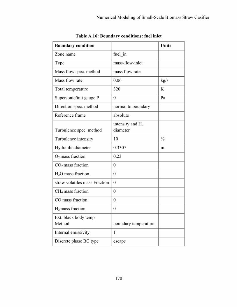
Numerical Modeling of Small-Scale Biomass Straw Gasifier
170
Table A.16: Boundary conditions: fuel inlet
Boundary condition Units
Zone name fuel_in
Type mass-flow-inlet
Mass flow spec. method mass flow rate
Mass flow rate 0.06 kg/s
Total temperature 320 K
Supersonic/init gauge P 0 Pa
Direction spec. method normal to boundary
Reference frame absolute
Turbulence spec. method intensity and H. diameter
Turbulence intensity 10 %
Hydraulic diameter 0.3307 m
O2 mass fraction 0.23
CO2 mass fraction 0
H2O mass fraction 0
straw volatiles mass Fraction 0
CH4 mass fraction 0
CO mass fraction 0
H2 mass fraction 0
Ext. black body temp Method boundary temperature
Internal emissivity 1
Discrete phase BC type escape
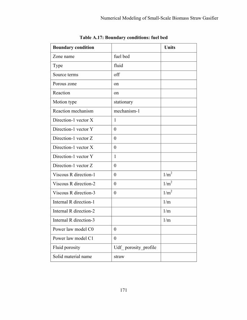
Numerical Modeling of Small-Scale Biomass Straw Gasifier
171
Table A.17: Boundary conditions: fuel bed
Boundary condition Units
Zone name fuel bed
Type fluid
Source terms off
Porous zone on
Reaction on
Motion type stationary
Reaction mechanism mechanism-1
Direction-1 vector X 1
Direction-1 vector Y 0
Direction-1 vector Z 0
Direction-1 vector X 0
Direction-1 vector Y 1
Direction-1 vector Z 0
Viscous R direction-1 0 1/m2
Viscous R direction-2 0 1/m2
Viscous R direction-3 0 1/m2
Internal R direction-1 1/m
Internal R direction-2 1/m
Internal R direction-3 1/m
Power law model C0 0
Power law model C1 0
Fluid porosity Udf_ porosity_profile
Solid material name straw

Numerical Modeling of Small-Scale Biomass Straw Gasifier
172
Table A.18: Boundary conditions: outlet
Boundary condition
Zone name outlet
Type outflow
Flow rate weighting 1
Ext. black body temp method
boundary temperature
Internal emissivity 1
Discrete phase BC type escape
Table A.19: Boundary conditions: default-interior
Boundary condition
Zone name default-interior
Type interior
Boundary condition
Zone name default-interior:008
Type interior
Boundary condition
Zone name default-interior:010
Type interior

Numerical Modeling of Small-Scale Biomass Straw Gasifier
173
Table A.20: Boundary conditions: walls
Boundary condition Units
Zone name wall
Type wall
Adjacent cell zone air
Thermal conditions heat flux
Heat flux 0 W/m2
Internal emissivity 0.5
Wall thickness 0 m
Heat generation rate 0 W/m3
Material name calcium sulphate
Boundary Condition Units
Zone name wall:001
Type wall
Adjacent cell zone fuel bed
Thermal conditions heat flux
Heat flux 0 W/m2
Internal emissivity 0.5
Wall thickness 0 m
Heat generation rate 0 W/m3
Material name calcium-sulphate

Numerical Modeling of Small-Scale Biomass Straw Gasifier
174
Table A.21: Solution controls
Solution controls
Pressure-velocity coupling SIMPLE
Skewness correction 0
Pressure URF 0.08
Density URF 0.08
Body Force URF 0.08
Momentum URF 0.08
Turbulent kinetic energy URF 0.1
Turbulent dissipation rate URF 0.1
Turbulent viscosity URF 0.1
O2 URF 0.1
CO2 URF 0.1
H2O URF 0.1
straw_vol URF 0.1
CH4 URF 0.1
CO URF 0.1
H2 URF 0.1
Energy URF 0.1
P1 URF 0.1
Discrete phase sources URF 0.1
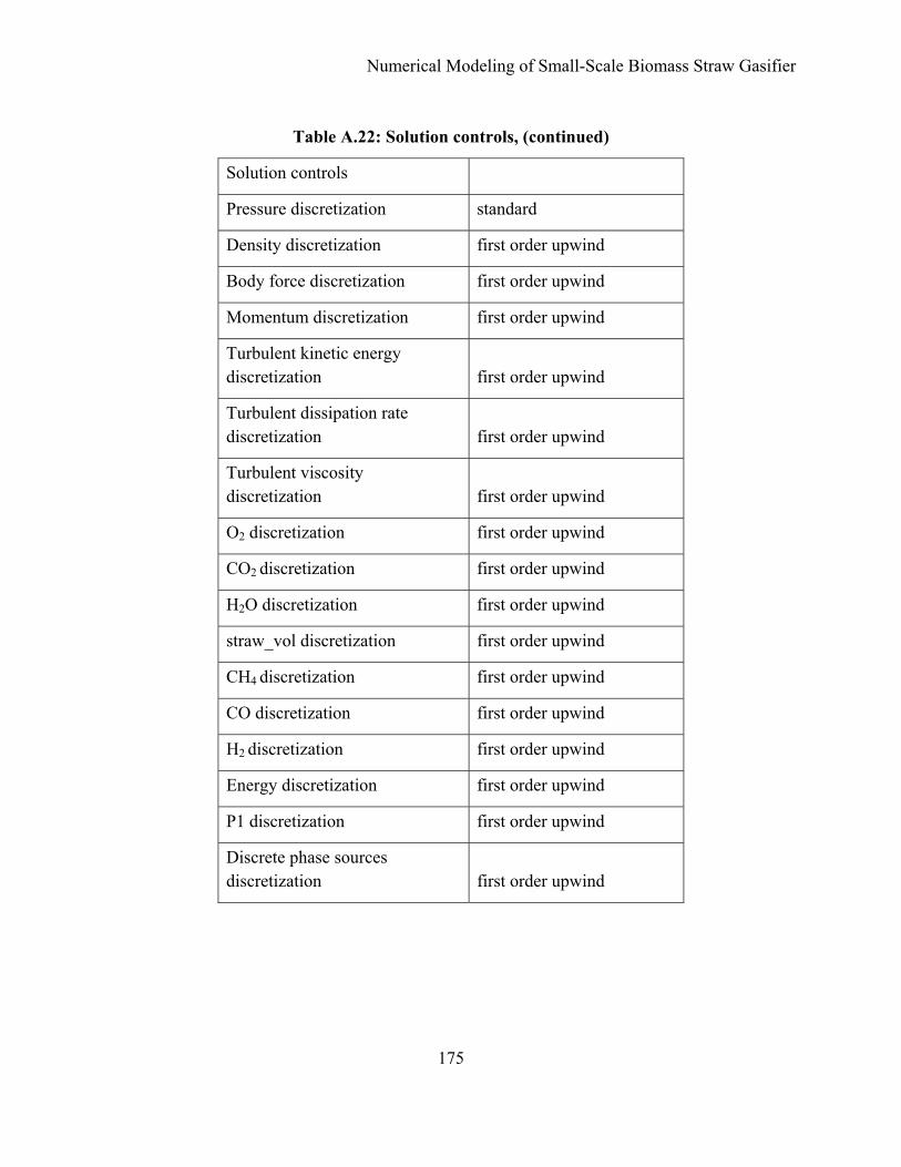
Numerical Modeling of Small-Scale Biomass Straw Gasifier
175
Table A.22: Solution controls, (continued)
Solution controls
Pressure discretization standard
Density discretization first order upwind
Body force discretization first order upwind
Momentum discretization first order upwind
Turbulent kinetic energy discretization first order upwind
Turbulent dissipation rate discretization first order upwind
Turbulent viscosity discretization first order upwind
O2 discretization first order upwind
CO2 discretization first order upwind
H2O discretization first order upwind
straw_vol discretization first order upwind
CH4 discretization first order upwind
CO discretization first order upwind
H2 discretization first order upwind
Energy discretization first order upwind
P1 discretization first order upwind
Discrete phase sources discretization first order upwind
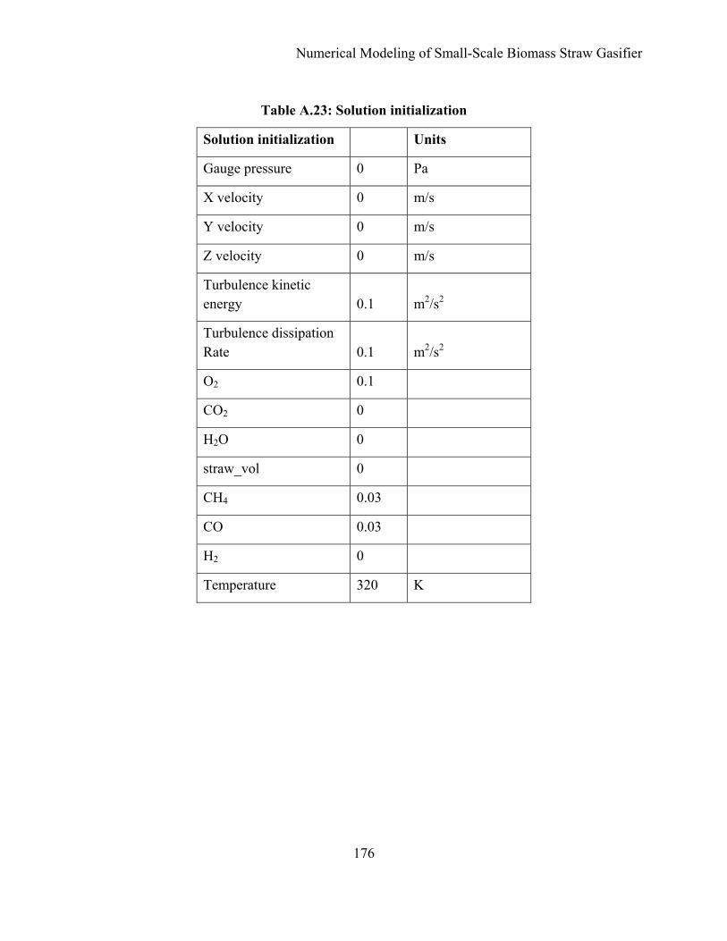
Numerical Modeling of Small-Scale Biomass Straw Gasifier
176
Table A.23: Solution initialization
Solution initialization Units
Gauge pressure 0 Pa
X velocity 0 m/s
Y velocity 0 m/s
Z velocity 0 m/s
Turbulence kinetic energy 0.1 m2/s2
Turbulence dissipation Rate 0.1 m2/s2
O2 0.1
CO2 0
H2O 0
straw_vol 0
CH4 0.03
CO 0.03
H2 0
Temperature 320 K

Numerical Modeling of Small-Scale Biomass Straw Gasifier
177
Table A.24: Residual controls
Residual Monitors
Continuity 1.00E-05
x-velocity 1.00E-05
y-velocity 1.00E-05
z-velocity 1.00E-05
energy 1.00E-05
k 1.00E-05
ε 1.00E-05
O2 1.00E-05
CO2 1.00E-05
CO2 1.00E-05
H2O 1.00E-05
straw_vol 1.00E-05
CH4 1.00E-05
CO 1.00E-05
H2 1.00E-05
P1 1.00E-06

Numerical Modeling of Small-Scale Biomass Straw Gasifier
178
Appendix B. Sampling protocol for emission testing
1. Biomass Analysis
1.1 Principle
Before gasification of the biomass begins, a sample of the biomass being tested was collected. A
sample was sent to a proper lab where an approximate and ultimate analysis was done. The
calorimetric value of the biomass and its moisture content was determined.
1.2 Apparatus
Ziploc Bag: - a clean Ziploc bag large enough to accommodate the biomass sample.
1.3 Procedure
A sample of approximately one liter was required for the proper analysis. It was essential that
the sample is representative of the biomass being gasified (i.e. All parts of the plant must be
represented in the sample). It was important to place the biomass in a clean Ziploc bag to avoid
the loss of any volatiles before analysis.
2. Producer gas sampling
2.1 Principle
A sample of gas produced during the gasification of biomass was collected in a Tedlar bag. The
composition, heating value and molecular weight of the gas was determined in the lab. Sensors
were in place to measure the gas temperature and flow rate at the sampling location.
2.2 Apparatus
Sample Probe: a probe made from any material that is resistant to the high temperature gas
stream at the sampling location. The material must also be inert to all components within the gas
stream. Because there were no foreseeable corrosion problems, standard industrial steel was
suitable. The probe diameter had to be between ¼” and 3/8”. The length of the probe depended
upon the exit temperature of the gas. The sample probe had to be of long enough to cool the gas

Numerical Modeling of Small-Scale Biomass Straw Gasifier
179
below 120°F or within the limits of the Tedlar bag system. If high exit gas temperatures were
anticipated, the sample probe needed to be water-cooled. For stack temperatures that exceed
800oF, a quartz probe could be used. The probe diameter had to be between ¼” and 3/8”. The
length of the probe is dependent upon the exit temperature of the gas. The sample probe must be
of sufficient length to be capable of cooling the gas below 50°C or within the limits of the Tedlar
bag system. The probe entrance had to be enlarged to approximately 20 mm I.D. for a length of
10 cm. The downstream end should be fitted with a 90o elbow and a ball joint. The probe had be
heat-traced and insulated if necessary to prevent sample condensation.
Thermocouple: a calibrated thermocouple capable of measuring the gas temperature within 2%
of the absolute gas temperature. A K-type ungrounded thermocouple 12” in length and with a
diameter of ¼” was selected. The thermocouple had a stainless steel sheath and ceramic
connector that allowed it to withstand high temperature gas stream.
Digital multimeter: capable of reading voltage, current and resistance and has a type-K input for
the thermocouple use.
Pitot tube: a Stauscheibe (type-S) with a known coefficient which is constant within ± 5% over
the entire working range.
Pressure Gauge: an inclined Manometer in the same range as the velocity and static pressures
being measured in the stack. It had to be capable of measuring the pitot tube velocity pressure
and the pressure drop across the orifice to within 0.1 mm (0.005 in) H20 on the 0 to 25 mm (1 in)
H20 scale and 1 mm (0.05 in) H20 on the 25-250 mm (1 -10 in) H20 scale.
Vacuum chamber: a heavy-duty vacuum tight case to accommodate a 10 L size Tedlar sample
bag. The chamber must be at a negative pressure to fill the sample bag directly.
Sample bag: a bag of non-reactive Tedlar material with a capacity of 10 L. Teflon tubing with a
diameter that could accommodate the sample bag was required.
Personal sampling pump: a pump capable of maintaining a sampling rate of 1 L/min to 2 L/min
while withdrawing a portion of the stack gas through the sampling train. It had to be equipped
with a flexible connecting tube to attach to the chamber.

Numerical Modeling of Small-Scale Biomass Straw Gasifier
180
2.3 Procedure
It was important to run the gasifier for at least 20 min before a gas sample could be collected and
make sure it was running at a constant and proper load. Temperature and flow rate sensor
preparation required that the faces of both openings were perpendicular to the airflow
(Figure B.1).
Figure B.1: S-type pitot tube specifications and orientation
Proper thermocouple placement to prevent interference was required while assembling the pitot
tube and thermocouple (Figure B.2). Dt had to be between 0.48 cm and 0.95 cm (3/16 in and 3/8
in).

Numerical Modeling of Small-Scale Biomass Straw Gasifier
181
Figure B.2: Pitot tube and thermocouple placement
It was also important to properly assemble the Pitot tube and the sampling probe as shown on
Figure B.3.
Figure B.3: Assembling pitot tube and sampling probe
The minimum pitot-sample probe separation needed to prevent interference was also given by
Dt, where Dt had to be between 0.48 cm and 0.95 cm (3/16 in and 3/8 in). Figure B.4 shows the
assembling of probe with pitot tube and thermocouple.
Figure B.4: Probe with pitot tube and thermocouple
The next step was to prepare the vacuum chamber using the following two steps:

Numerical Modeling of Small-Scale Biomass Straw Gasifier
182
• Insert a 10 L tedlar bag inside the vacuum chamber and connect it to the sample
valve.
• On the outside of the chamber, connect the Teflon tubing to the sample valve.
This was the sampling line that attached to the open end of the sample probe.
Finally, the sample port location and specifications had to be determined. To obtain accurate
results when sampling a gas stream, the location of the sampling port was important. A location
where the gas flow was well mixed and the infiltration of ambient air is at a minimum is
preferred. The flow of the gas stream is also required to be laminar with no cyclonic or
stratification patterns at the sampling location.
To meet the following criteria, the sample port had to be located in a straight section of the pipe.
It had to be located eight or more stack diameters in length downstream and two or more stack
diameters upstream from any flow disturbance (bend, elbow, etc.). Figure B.5 below illustrates
the minimum standards that must be met for the location of the sample port.
Figure B.5: a) Location of sample port and b) Distance away from duct wall

Numerical Modeling of Small-Scale Biomass Straw Gasifier
183
The sampling port was made from standard industrial pipe, because there were no foreseeable
corrosion problems. The inside diameter of the port has be at least 3- ½ in. and extend 3 inches
outwards from the exterior stack of the wall. The port had to be threaded to be able to
accommodate a cap. The cap had to be used when the port is not being used.
3. Gas sampling
The sampling procedures were as follows:
1. Attach the sample line to the pump inlet valve on the vacuum chamber.
2. Wait for 15–30 s for the sample line to fill with the producer gas and then reattach the
sample line to the sample valve.
3. Attach the personal sampling pump to the chamber In/Out valve and start the sample
pump at a rate between 1 L/min and 2 L/min.
4. Make sure that the sampling rate is recorded and held constant throughout the sampling.
5. When the bag is ¾ full, disconnect the sample line and shut off the sample pump.
It was important to measure and record temperature and flow rate throughout sampling using the
digital multimeter and manometer.
10 L Tedlar Bag
Teflon Tubing
Pump
Vacuum Chamber
Digital Multimeter
Manometer
Pitot Tube
Thermocouple
Sample Probe
Figure B.6: Producer gas sample train

Numerical Modeling of Small-Scale Biomass Straw Gasifier
184
4. Sampling of PM
4.1 Introduction
Particulate matter is not an absolute quantity; rather, it is a function of temperature and pressure.
Therefore, to prevent variability in particulate matter emission regulations and/or associated test
methods, the temperature and pressure at which particulate matter was to be measured had to be
carefully defined. Of the two variables (i.e., temperature and pressure), temperature had the
greater effect on the amount of particulate matter in an effluent gas stream; in most stationary
source categories, the effect of pressure appeared to be negligible. In Method E of Environment
Protection Agency (EPA) standard, 120oC ± 14oC (250oF ± 25oF) was established as a nominal
reference temperature. Thus, where Method 5 was specified in an applicable subpart of the
standards, particulate matter was defined with respect to temperature. To maintain a collection
temperature of 120oC ± 14oC (250oF ± 25oF), Method 5 employed a heated sample probe and a
heated filter holder.
4.2 Principle
Particulate matter was withdrawn isokinetically from the source and collected on a glass fiber
filter maintained at stack temperature. The particulate mass was determined gravimetrically after
uncombined water was removed.
4.3 Applicability
This method applied to the determination of particulate emissions from stationary sources for
determining compliance with new source performance standards, only when specifically
provided for in an applicable subpart of the standards. This method was not applicable to stacks
that contain liquid droplets or were saturated with water vapor.
4.4 Apparatus
The sampling train consisted of a sample probe, thermocouple, digital multimeter, pitot tube, and
pressure gauge with the same type and specification used in the producer gas sampling train. In
addition, the following apparatus were used.

Numerical Modeling of Small-Scale Biomass Straw Gasifier
185
Nozzle: -a nozzle constructed of stainless steel or quartz and connected to a heated glass probe
liner with a sharp, tapered leading edge. The angle of the taper had to be 30o and the taper had to
be on the outside to preserve a constant internal diameter. The probe nozzle shall be of the
button-hook or elbow design. Nozzle diameters had to be sized to allow for isokinetic sampling.
Filter holder: a Teflon-coated stainless steel filter holder containing a quartz glass filter.
The probe line was connected to a Teflon-coated stainless steel filter holder containing a quartz
glass filter. The filter had to be heated in a hot box to 120oC ± 14oC (250oF ± 25oF). The back
half of the filter holder was connected to a series of impingers with insulated Teflon tubing.
Heating compartment heating system: a heating system capable of maintaining the temperature
of the filter holder compartment at 120oC ± 14oC (25oF ± 25oF) was needed. A temperature
gauge accurate to within 3oC (5.4oF) shall be installed such that the temperature around the filter
holder could be monitored during sampling.
Impingers: one standard and three modified (the tips and impaction plates of the standard design
were replaced with a 13 mm (0.5 in) ID glass tube extending to within 13 mm (0.5 in) of the
bottom of the impinger) Greenberg-Smith impingers with vertical and side ports (Figure B.9).
Cooling system: an ice bath was used to contain the impingers in order to cool them.
Dry test meter: a 175 CFH dry test meter accurate within ± 2% of the true volume and equipped
with a thermometer to measure the inlet and outlet temperature.
Vacuum Pump: a leak-free vacuum pump capable of maintaining a 28.7 L/min (1.0 CFM) flow
rate at 380 mm Hg (15 inches of mercury) or a sampling rate of 1-2 L/min while continuously
withdrawing a portion of the stack gases through the sampling train. The pump had to a sample
rate control valve and a vacuum gauge attached to the inlet.
Barometer: a barometer that was accurate to within 2.5mm Hg (± 0.1 inches of Hg).
Orifice: a calibrated orifice connected to the outlet of the dry gas meter.

Numerical Modeling of Small-Scale Biomass Straw Gasifier
186
Connections: the connection between the filter and the first impinger had to be able to withstand
stack temperatures. All connections leading up to the filter were to be constructed of Teflon
and/or borosilicate glass and/or quartz.
Analytical Balance: an analytical balance capable of measuring condensate weights to the nearest
0.1 gram is acceptable.
4.5 Pre- Sampling Procedure
Prior to sampling, traverse points were selected on the basis of EPA Method A requirements.
Then, Pitot tube, thermocouple and the sample nozzle were assembled properly as shown on
Figure B.7.
Figure B.7: Pitot tube-sampling nozzle
Proper pitot tube-sampling nozzle configuration to prevent aerodynamic interference was
required (Figure B.8) with button-hook type nozzle where centers of nozzle and pitot opening
aligned and with Dt between 0.48 cm and 0.95 cm (3/16 in and 3/8 in.).

Numerical Modeling of Small-Scale Biomass Straw Gasifier
187
Figure B.8: Pitot tube-sampling nozzle configuration
The sample nozzle was determined to the known moisture content of the flue gas. Next, the
impinger boxes and filters were assembled and weighed in an onsite trailer as illustrated in EPA
Method E (Figure B.9).
Modified Standard Train of 4 Impingers
Figure B.9: Impinger assembly
The first two impingers were charged with approximately 100 mL of deionized or distilled water
while leaving the third impinger dry and the fourth to be charged with a known amount
(approximately 200 g) silica gel to remove any residual water.

Numerical Modeling of Small-Scale Biomass Straw Gasifier
188
The volume or weight of each impinger was recorded on the moisture analysis data sheet. The
total weight was given by
Weight of total water collected= [a] + [b] +[c] + [d] g
Finally, the sampling train was set up as illustrated in EPS Method E (Figure B.10) first by
adjusting the filter compartment and the probe heating systems to maintain a temperature of
120oC ± 14oC (250oF ± 25oF) to prevent the blinding of the filter due to condensation.
Figure B.10: Sampling train set up
Then, a mandatory pre-test leak check of the sampling train was conducted by plugging the
nozzle inlet and pulling a vacuum of 380 mm Hg (15 in Hg) for at least one minute. The leakage
rate had to be < 0.57 L/min (0.002 ft3/min) or 4 % of the estimated average sampling rate,
whichever was less.
4.6 Sampling operation
The following steps were performed to do the sampling operation.
1. Clean the portholes prior to the test run to minimize the chance of sampling the
deposited material. To begin sampling, remove the nozzle cap and verify that the
Pitot tube and probe extension are properly positioned.

Numerical Modeling of Small-Scale Biomass Straw Gasifier
189
2. Position the nozzle at the first traverse point with the tip pointing directly into the
gas stream.
3. Immediately start the pump and adjust the flow to isokinetic conditions.
Nomographs are available, which aid in the rapid adjustment to the isokinetic
sampling rate without excessive computations. These nomographs are designed for
use when the type S-pitot tube coefficient is 0.85 ± 02, and the stack gas equivalent
density (dry molecular weight) is equal to 29 ± 4.
4. Sample for at least five min at each traverse point, the sampling rate being the same
for every point.
5. Traverse the stack cross-section and maintain isokinetic sampling throughout the
test.
6. When it is necessary to halt sampling temporarily to dismantle the sampling train
during port changeover or to change a train component, turn off the pump and
immediately withdraw the probe from the stack.
7. Conduct a mandatory post-test leak-check on the sampling train by plugging the
nozzle and pulling a vacuum equal to or greater than the maximum value observed
during sampling.
8. If the leakage rate is >0.57 L/min (0.002 ft3/min) or 4% of the estimated average
sampling rate, the test is invalid.
The following steps have to be considered for a successful operation.
1. Add more water and ice to the impinger box, as required, to maintain the
temperature of the last impinger exit in the range of 0ºC -20ºC.
2. Record instrumentation readings every 5 min (sampling duration), before and after
a leak check and when sampling is halted.
3. If, during the sampling run, a component (e.g., filter assembly or impinger) change
becomes necessary, a leak-check shall be conducted immediately before the change
is made.
Numerical Modeling of Small-Scale Biomass Straw Gasifier
190
5. Residual ash collection
5.1 Principle
Upon completion of gasification, a sample of the residual ash produced was collected. The
sample was analyzed and its composition determined. The mass of the total amount of residual
ash produced from the biomass was determined. From this information, the amount of ash that
became residual ash and the amount that became fly ash during gasification could be determined.
5.2 Apparatus
Ziploc bag: a clean Ziploc bag that was the proper size for the residual ash sample.
Scoop/shovel: a small scoop or shovel that could fit in the ash disposal area and collect a proper
sample of the residual ash.
Small scale: a scale capable of weighing 0.1 mg.
5.3 Procedure
All gasifiers have an area where a large portion of the ash collected during gasification. To avoid
contamination of the sample, this area had to be thoroughly cleaned before testing could occur.
Most of the ash was removed first with the compressed air hose and/or a shovel.
For small gasifiers or smaller biomass sample sizes, about 10% of the total residual ash produced
was to be collected (around 200 g). When collecting the sample it was important that the ash
collected represented the ash produced by the gasifier. A homogeneous, well mixed sample
should be taken. It could be scooped out of the ash disposal area and placed into the Ziploc bag.
The Ziploc bag was to be stored at room temperature in a dry area till the analysis can be
preformed.
Calibration of measuring devices was required and the results had to be recorded. The following
instruments needed to be calibrated.
Probe Nozzles: - probe nozzles had to be calibrated before their initial use in the field. Using a
micrometer, the inside diameter of the nozzle was measured to the nearest 0.025 mm (0.001 in.).
Three separate measurements using different diameters each time was required, and the average

Numerical Modeling of Small-Scale Biomass Straw Gasifier
191
of the measurements was obtained. The difference between the high and low numbers should not
exceed 0.1 mm (0.004 in.). When nozzles become nicked, dented, or corroded, they should be
reshaped, sharpened, and recalibrated before use. Each nozzle had to be permanently and
uniquely identified.
Pitot tube: if the pitot tube was placed in an interference-free arrangement with respect to the
other probe assembly components, its baseline (isolated tube) coefficient had be determined
Metering system: the metering system included a vacuum gauge, leak-free pump, thermometers
capable of measuring temperature to within 3oC (5.4oF), dry gas meter capable of measuring
volume to within 2 percent. Before its initial use in the field, the metering system had to be
calibrated according to the procedure outlined in APTD-0576. Instead of physically adjusting the
dry gas meter dial readings to correspond to the wet test meter readings, calibration factors could
be used to mathematically correct the gas meter dial readings to the proper values.
Before calibrating the metering system, it was suggested that a leak-check be conducted. For
metering systems having diaphragm pumps, the normal leak-check procedure would not detect
leakages within the pump. For these cases the following leak-check procedure was suggested:
make a 10-minute calibration run at 0.00057 m3/min (0.02 cfm); at the end of the run, take the
difference of the measured wet test meter and dry gas meter volumes; divide the difference by
10, to get the leak rate. The leak rate should not exceed 0.00057 m3/min (0.02 cfm).
After each field use, the calibration of the metering system had to be checked by performing
three calibration runs at a single, intermediate orifice setting (based on the previous field test),
with the vacuum set at the maximum value reached during the test series. To adjust the vacuum,
insert a valve between the wet test meter and the inlet of the metering system. Calculate the
average value of the calibration factor. If the calibration changed by more than 5 percent,
recalibrate the meter over the full range of orifice settings.
If the dry gas meter coefficient values obtained before and after a test series differ by more than
5 percent, the test series had to either be voided, or calculations for the test series had be
performed using whichever meter coefficient value (i.e., before or after) gave the lower value of
total sample volume.

Numerical Modeling of Small-Scale Biomass Straw Gasifier
192
Temperature gauges: dial thermometers, such as those used for the dry gas meter and condenser
outlet had to be calibrated against mercury-in-glass thermometers.
Leak check of metering system: the portion of the sampling train from the pump to the orifice
meter should be leak checked prior to initial use and after each shipment.
Figure B.11: Leak free check
Leakage after the pump would result in less volume being recorded than is actually sampled. The
following procedure was suggested (see Figure B.11). Close the main valve on the meter box.
Insert a one-hole rubber stopper with rubber tubing attached into the orifice exhaust pipe.
Disconnect and vent the low side of the orifice manometer. Close off the low side orifice tap.
Pressurize the system to 13 to 18 cm (5 to 7 in.) water column by blowing into the rubber tubing.
Pinch off the tubing and observe the manometer for one minute. A loss of pressure on the
manometer indicates a leak in the meter box; leaks, if present, must be corrected.
Barometer: wass calibrated against a mercury barometer.

Numerical Modeling of Small-Scale Biomass Straw Gasifier
193
Appendix C. Measurements of gas composition report
1. Emission source
Gasification is a process by a solid carbonaceous material, containing mostly chemically bound
carbon, hydrogen, oxygen, and a variety of inorganic and organic constituents, is reacted with air
and oxygen. The reactions provide sufficient exothermic energy to produce a primary gaseous
product containing mostly CO, H2, CO2, H2O (gas), and light hydrocarbons laced with volatile
and condensable organic and inorganic compounds. Most of the inorganic constituents in the
feedstock are chemically altered and either discharged as bottom ash or entrained with the raw
product gas as fly-ash. The gasifier features a first stage of updraft gasification followed by a
second stage of downdraft char gasification. The second stage also serves to crack the tars
contained in the first stage producer gas as a result of the updraft gasification of the wet wheat
straw.
2. Method and references
The measurement was undertaken using the Model 375K / 375WP – portable flue gas analyzer
(Figure C.1) manufactured by Nova Analytical Systems Inc in accordance with the main
procedural requirements given within the acceptable Canadian standard methods as tabulated in
Table C.1.
Table C.1: Applicable methods and references
Method # parameter
EPA Method A traverse points
EP A Method B velocity & flow rate
EPA Method C gas molecular weight
EPA Method D gas moisture
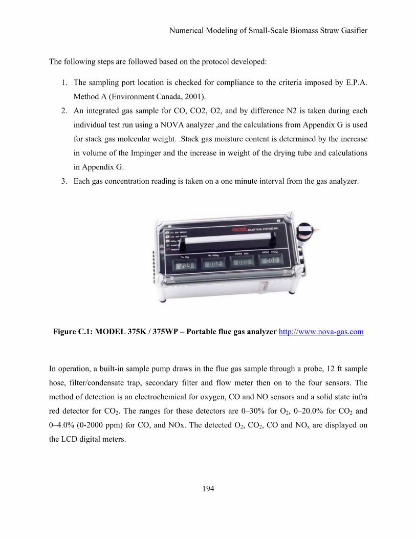
Numerical Modeling of Small-Scale Biomass Straw Gasifier
194
The following steps are followed based on the protocol developed:
1. The sampling port location is checked for compliance to the criteria imposed by E.P.A.
Method A (Environment Canada, 2001).
2. An integrated gas sample for CO, CO2, O2, and by difference N2 is taken during each
individual test run using a NOVA analyzer ,and the calculations from Appendix G is used
for stack gas molecular weight. .Stack gas moisture content is determined by the increase
in volume of the Impinger and the increase in weight of the drying tube and calculations
in Appendix G.
3. Each gas concentration reading is taken on a one minute interval from the gas analyzer.
Figure C.1: MODEL 375K / 375WP – Portable flue gas analyzer http://www.nova-gas.com
In operation, a built-in sample pump draws in the flue gas sample through a probe, 12 ft sample
hose, filter/condensate trap, secondary filter and flow meter then on to the four sensors. The
method of detection is an electrochemical for oxygen, CO and NO sensors and a solid state infra
red detector for CO2. The ranges for these detectors are 0–30% for O2, 0–20.0% for CO2 and
0–4.0% (0-2000 ppm) for CO, and NOx. The detected O2, CO2, CO and NOx are displayed on
the LCD digital meters.

Numerical Modeling of Small-Scale Biomass Straw Gasifier
195
3. Measuring location
The test site was visited prior to undertaking the sampling procedure, even if testing had
previously been undertaken at the site. During this visit, the two 3 inch diameter sample ports
were found ideally located (8 and 2 diameter criteria) on the 12-inch diameter exhaust stack. In
addition, the permanent working platform, its access and safety precautions were found to be
satisfactory.
4. Results
Under continuous operating conditions, five measurement readings were carried out for each
moisture content of wheat straw to assess the concentration of gases from the exhaust stack. The
operation conditions for the whole period of measuring are in Appendix E. The readings for all
four gases, O2, CO2, CO and NOx, are also in Appendix E. The summary of the results obtained
from this testing is tabulated below in Table C.2.
Table C.2: Summary of combustion gas concentration
Vidir Best gasifier, exhaust stack, Arborg, MB
Date Moisture content %
O2 CO CO2 NOx
July 10th, 2007
% mg/m3 ppm mg/m3 % mg/m3 ppm mg/m3
14 6.34 829.8 100.0 114.5 15.58 2803.8 533.0 1002
26 7.26 950.2 157.8 180.7 14.66 2638.2 541.6 1017
20 2.96 387.4 3340.0 3824.9 18.18 3271.7 261.6 492

Numerical Modeling of Small-Scale Biomass Straw Gasifier
196
Appendix D. Measurement of particulate emission sampling and
testing
On 07 June 2006, particulate emission testing was undertaken by University of Manitoba, on the
Vidir Best plant at Vidir Machine Inc., MB. During the test, the weather was noted as dry and
sunny with an ambient air temperature of 30oC (86oF). The purpose of the emission testing was
to quantify the total suspended particulate matter for the following reasons:
• to determine if a process unit complied with existing or proposed emission
regulations
• to ascertain the economics of materials or product losses from a source
• to obtain relevant data which could facilitate the selection and design of control
equipment
• to test the efficiency of installed control equipment
• to allow control of a process by continuous or frequent observation of one or more
constituents in the stack gas stream
• to provide more accurate data to develop air resources management programs,
control regulations and inventories
These measured emission rates were conducted with the gasifier operating with an approximate
feed rate of 500 lb/hr (227 kg/hr) of wheat straw.
1. Introduction
Emissions testing (i.e., stack sampling or stack monitoring, etc.) is the experimental process for
evaluating the characteristics of industrial waste gas stream emissions into the atmosphere.
Materials emitted to the air from these sources can be solid, liquid, or gas; organic or inorganic.
The effluent pollutants emitted to the atmosphere from a source may contain many different
pollutant materials. Effluent measurements and sampling procedures follow specific test methods
and protocols to ensure representative and accurate emission data. Test methods are pollutant
specific, sometimes industry specific, and originate from a variety of sources and jurisdictions

Numerical Modeling of Small-Scale Biomass Straw Gasifier
197
such as USEPA, Environment Canada, state agencies, provincial agencies, trade organizations,
etc.
2. Sampling and testing
2.1 Emission source
Gasification is a process by which a solid carbonaceous material, containing mostly chemically
bound carbon, hydrogen, oxygen, and a variety of inorganic and organic constituents, is reacted
with air and oxygen. The reactions provide sufficient exothermic energy to produce a primary
gaseous product containing mostly CO, H2, CO2, H2O (g), and light hydrocarbons laced with
volatile and condensable organic and inorganic compounds. Most of the inorganic constituents in
the feedstock were chemically altered and either discharged as bottom ash or entrained with the
raw product gas as fly-ash.
2.2 Test method and references
Isokinetic sampling of the contained emission sources was undertaken using the CLEAN AIR
EXPRESS® Instruments Inc Method 5 Isokinetic sampling apparatus in accordance with main
procedural requirements and within the following acceptable Canadian standard methods (Table
D.1)
Table D.1: Applicable methods and references
Method # Parameter
EPA Method A traverse points
EP A Method B velocity & flow rate
EPA Method C gas molecular weight
EPA Method D gas moisture
EPA Method E (1 to 8) particulate matter
All measuring devices including, but not limited to, pitot tubes, meters, gauges, and
thermocouples were properly calibrated and maintained to provide accurate data. The sampling

Numerical Modeling of Small-Scale Biomass Straw Gasifier
198
location and number of traverse points were determined by EPA Method A. EPA Method B and
equations in Appendix G were used to determine stack gas velocity. An integrated gas sample
for CO, CO2, O2, and by difference N2 was taken during each individual test run using a Nova
analyser manufactured by Nova Analytical Systems Inc and the calculations from Appendix G
were used for stack gas molecular weight. Then, stack gas moisture content determined by the
increase in volume of the impinger and the increase in weight of the drying tube is calculated.
Each performance test consisted of three separate and valid one-hour test runs and for the
purpose of determining compliance with any applicable standard; the results of each valid test
run (Appendix F) were considered.
2.3 Sampling Location
The site was visited prior to undertaking the sampling procedure, even if testing had previously
been undertaken at the site. During this visit, the two three-inch diameter sample ports were
found to be ideally located (8 and 2 diameter criteria) on the 12-inch diameter exhaust stack. In
addition, the permanent working platform, its access and safety precautions were found to be
satisfactory.
2.4 Sample Train
The Clean Air Express Method 5 Train (Figure D.1) is which is the benchmark of the industry,
was used to do the sampling. It is suited to perform isokinetic particulate testing referencing
federal EPA 40 CFR 60, Appendix A, Method E “Determination of Particulate Emissions from
Stationary Sources.”

Numerical Modeling of Small-Scale Biomass Straw Gasifier
199
Figure D.1: Method 5 isokinetic sampling Train (http://www.cleanair.com)

Numerical Modeling of Small-Scale Biomass Straw Gasifier
200
The parts that are consisted in the sampling train are listed in table.
Table D.2: Clean Air Express® Method 5 train
1 Isokinetic control console with pump
2 Sample oven compartment
3 Impinger compartment
4 3” Glassware kit Ball joint or ball joint O-Ring
5 Stainless steel impinger outlet
6 50’ Umbilical cable with stainless steel quick connects
7 6’ Stainless steel heated Method 5 probe with liner and geometric calibration report
8 Stainless steel probe port adaptor seal assembly
9 Complete set of stainless steel nozzles (1/8” 3/16” 1/4" 5/16” 3/8”, and 1/2") with nuts
and ferrules
10 Sample recovery kit
11 8.5 cm glass fiber filters (box of 100)
2.5 Sampling Procedure
Isokinetic source sampling is achieved when the velocity of gas entering the sampling nozzle is
exactly equal to the velocity of the approaching gas stream. This provides a uniform, unbiased
sample of the pollutants being emitted by the source. Isokinetic source sampling most closely
evaluates and defines various parameters in the stack as they actually exist at the time of
sampling. Preliminary measurements were made in order to determine the appropriate sized
nozzle for isokinetic sampling across the velocity profile of the stack. Minor adjustments
required to maintain an isokinetic condition at each test point were accomplished by regulating
the sample flow rate.

Numerical Modeling of Small-Scale Biomass Straw Gasifier
201
2.6 Sample collection
A leak check was carried out before and after sampling to confirm all the suction is had been
drawn through the nozzle. With the required isokinetic flow rates known, the sample probe is
inserted into the stack at 90o to the gas flow so that any particulate matter impinging on the filter
before sampling could be stopped. The filter head and probe were allowed to reach the stack gas
temperature. The initial gas meter volume was noted and the suction device and timer started.
The correct flow rate for isokinetic sampling is set and the nozzle positioned to face parallel to
the gas flow. Sampling was then carried out for the planned duration and number of sample
points, recording all the necessary data for final calculations. On completion, the suction device
and the timer were stopped and the final gas meter volume recorded. The probe was removed
from the process stack and a further leak test carried out before removing the filter, which was
subsequently removed and placed in a storage container. In addition, any residual particulate
upstream of the filter was washed with water and acetone into an appropriate beaker.
The above procedures were then repeated to obtain duplicate samples. At all times during the
sampling procedure the sampling person was in contact with the process operator to ensure that
the plant was in full production and there were no changes in the process that might affect the
representative nature of the samples collected.
2.7 Validation of test
Main conditions for compliance with ISO 9096:2003 are listed below. A single tick in the "fail"
column indicates that this test did not comply with the full provisions of ISO 9096:2003. Due to
site/sampling locations it was not always practically possible for all the conditions to be met.
Best practical means were employed to try to achieve a representative result.

Numerical Modeling of Small-Scale Biomass Straw Gasifier
202
Table D.3: Test validation chart
Preliminary Velocity Survey Pass Fail
Direction of gas flow within 15o of flue axis *
Pitot-static pressure differential greater than 5 Pa (3 m/s) *
Ratio of highest to lowest pitot-static readings less than 9:1 *
Sampling procedure *
Sampling plane is correctly positioned *
Sampling centroids of equal area *
Nozzle is facing upstream to within + 10o *
Leak check performed *
Constant 'at' during cumulative sampling *
Post sampling operations *
Leak test performed *
Isokinetic rate 90% to 110 % * *
*Any test run during which the average percent isokinetic sampling rate (Appendix F) is less
than 90% or greater than 110% considered to be invalid.
2.8 Preliminary sampling results
Three articulate tests were carried out for the different moisture content of the given biomass,
under continuous operating conditions, to assess the emission concentration in the exhaust gases.
The sample time of each test was one hour after which the samples were recovered from the
sampling train and sent for an analysis to the Norwest Lab, Winnipeg, MB.

Numerical Modeling of Small-Scale Biomass Straw Gasifier
203
Table D.4: Operating conditions during the measurement (14% moisture)
Average operating conditions obtained from Vidir Smartfire remote monitor
data logging (14% moisture)
Moisture
content
14%
primary
chamber
temp [oF]
secondary
chamber
temp [oF]
boiler temp
[oF]
boiler in
temp [oF]
exhaust
temp [oF]
1055.8
21389.0
141.8
114.1
364.9
Flue gas
oxygen %
system_
pressure
[psi]
primary
air inflow
[ft/sec]
primary air in
temp. [oF]
secondary
air inflow
[ft/sec]
secondary
air in temp.
[oF]
5.9
-1.1
7.7
71.3
5.3
73.9
Table D.5: Operating conditions during the measurement period (26% moisture).
Average operating conditions obtained from Vidir Smartfire remote monitor
data logging (26% moisture content)
Moisture
content
26%
primary
chamber
temp [oF]
secondary
chamber
temp [oF]
boiler temp
[oF]
boiler in
temp [oF]
exhaust
temp [oF]
1148.1
2014.5
137.5
110.0
380.5
Flue gas
oxygen %
system_
pressure
[psi]
primary
air inflow
[ft/sec]
primary air in
temp [oF]
secondary
air inflow
[ft/sec]
secondary
air in temp
[oF]
5.0
–1.0
11.5
67.9
17.4
70.3

Numerical Modeling of Small-Scale Biomass Straw Gasifier
204
Table D.6: Operating conditions during the measurement (20% moisture)
Average operating conditions obtained from Vidir Smartfire remote monitor
data logging (20% moisture content)
Moisture
content
20%
primary
chamber
temp [oF]
secondary
Chamber
temp [oF]
boiler temp
[oF]
boiler in
temp [oF]
exhaust
temp [oF]
948.1 2214.0 145.8 117.2 367.5
Flue gas
oxygen %
System_
pressure
[psi]
primary
air inflow
[ft/sec]
primary air in
temp [oF]
secondary
air inflow
[ft/sec]
secondary
air in temp.
[oF]
5.6 -1.0 9.8 69.9 5.5 72.3
3. Emission testing results
The results from the emission testing are summarized in Table D.7. The total particulate matter
ranged from 0.391–0.539 mg/m3 while the corresponding emission rates were between 0.189–
0.249 gr/s. The average concentration of the total particulate matter and emission rate for the
gasification of wheat straw using the Vidir Best gasifier were 0.443 mg/m3 and 0.211 gr/s
respectively.

Numerical Modeling of Small-Scale Biomass Straw Gasifier
205
Table D.7: Particulate emissions from Vidir Best gasifier exhaust
Result Summary of emission testing for Wheat Straw Area of stack 0.785375 ft2
Reference conditions T =298oK (25oC), P=101.325Kpa
Emission rate E[lb / hr]
Emission rate E[gr/s] Test No.
Us [ft/sec]
Mn [mg] Grain/dscf
Csd [mg/m^3]
Csd@ 12%CO2
Moisture content 14% 38.04 485.2 0.249 0.539 0.415 2.092 0.249 Moisture content 26% 39.68 359.8 0.185 0.400 0.308 1.436 0.192 Moisture content 20% 39.90 352.3 0.181 0.391 0.301 1.503 0.189 Average 39.21 399.1 0.205 0.443 0.334 1.669 0.211

Numerical Modeling of Small-Scale Biomass Straw Gasifier
206
Appendix E. Gas composition data sheets
Table E.1: Data recording sheet for wheat straw
Gas analysis (wheat straw moisture content = 14% ) Vidir Best, Arborg, MB
Sampling duration: every 12 min %CO2 %O2
(%N2+ %CO)
CO ppm NOx ppm
1 14.6 8 77.4 100 489
2 15.7 6.2 78.1 100 618
3 16.2 6.4 77.4 100 513
4 15.9 5.6 78.5 100 520
5 15.5 5.5 79 100 525
Average 15.58 6.34 78.08 100 533
Dry molecular Wt. (Md) 30.7464 lb/lb-mole
Wet molecular Wt. (Ms) 28.70698 lb/lb-mole

Numerical Modeling of Small-Scale Biomass Straw Gasifier
207
Table E.2: Gas analysis wheat straw of moisture content = 20% summary
Table E.3: Gas analysis for wheat straw of moisture content = 26% summary
Gas analysis (wheat straw of Moisture content = 20%) Vidir Best, Arborg, MB Sampling duration: every 12 min %CO2 %O2
(%N2 + %CO)
CO ppm NOx ppm
1 15 6.1 78.9 50 623 2 13.7 8.7 77.6 56 630 3 13.8 7.4 78.8 79 539 4 14.3 8.7 77 430 379 5 16.5 5.4 78.1 174 537 Average 14.66 7.26 78.08 157.8 541.6 Dry molecular Wt. (Md) is 30.636 lb/lb-mole Wet molecular Wt. (Ms) is: 28.61424 lb/lb-mole
Gas analysis (wheat straw of Moisture Content = 26%) Vidir Best, Arborg, MB
Sampling duration every 12min %CO2 %O2
(%N2 + %CO)
CO ppm NOx ppm
1 18.8 2.8 78.4 3500 190
2 18.3 2.9 78.8 2100 243
3 18.5 2.5 79 7300 298
4 17.5 4.3 78.2 2100 360
5 17.8 2.3 79.9 1700 217
Average 18.18 2.96 78.86 3340 261.6
Dry molecular Wt. (Md) 31.0272 lb/lb-mole
Wet molecular Wt. (Ms) 28.94285 lb/lb-mole

Numerical Modeling of Small-Scale Biomass Straw Gasifier
208
Appendix F. Particulate emission sampling and testing data
sheets
Table F.1: Preliminary stack test data sheet (Run 1)
Preliminary stack test data: wheat straw ( Run 1)
Company: Vidir Best Inc. Facility: Arborg
Location: Box 600, Arborg, MB Date: 07 /06 /07
Data collected by: Daniel Balcha Ambient temperature : 84oF
Equivalent stack diameter (in.): 12 Est. moisture: 0.16
Diameters downstream : 8 Stack temperature : 3250F
Diameters upstream: 2 Barometric: 29.9 in. Hg
Number of sample ports: 2 Static press: 29.9 in. Hg
Sampling points needed: 12 Average ΔH reading: 0.97 in. W.C.
Orifice: ΔH@: 1.727 Maximum √ΔP: 0.62 in. W.C.
Pitot: Cp : 1 Average. √ΔP: 0.595 in. W.C.
Nozzle Diameter: 0.25 in Estimated meter temperature 98oF
Meter: Y-factor : 1

Numerical Modeling of Small-Scale Biomass Straw Gasifier
209
Table F.2: Particulate emission sampling data recording sheet-MC = 14%
RUN # 1 Moisture Content 14%
Sample
Dry Gas
Meter
Pitot
ΔP Orifice Pump
Temperatures [oF]
Port &
Reading
[ft3]
in
H2O Pressure Vacuum DGM Stack Probe Filter
Imp.
Exit
point ΔH[inH2O] Inlet Outlet %Iso
Us
[fps]
1, 1 157.0 0.33 0.880 0 92 74 225 250 250 62 92.27 36.7
1, 2 159.6 0.33 0.860 3 93 76 267 255 249 67 94.79 37.8
1, 3 161.5 0.34 0.890 3 92 74 315 250 250 64 96.69 39.61
1, 4 165.4 0.34 0.800 4 93 73 289 248 250 68 95.04 38.9
1, 5 168.1 0.32 0.860 3 93 78 228 247 251 61 93.47 36.2
1, 6 170.5 0.32 0.870 4 92 77 310 252 252 58 99.07 38.3
2, 7 173.2 0.31 0.890 4 93 78 290 250 258 62 99.16 37.2
2, 8 175.7 0.33 0.880 4 92 74 285 251 256 63 96.23 38.3
2, 9 179.2 0.33 0.880 5 90 73 275 249 252 64 95.84 38.0
2, 10 182.6 0.34 0.870 4 93 75 265 247 251 66 93.35 38.3
2, 11 185.9 0.34 0.875 4 90 77 310 250 248 64 96.29 39.5
2, 12 188.2 0.33 0.880 4 93 78 265 250 253 65 94.49 37.7
AVER 0.33 0.870 3.5 92.2 75.6 277.0 249.9 251.7 63.7 95.56 38.0
Tot.Gas
Meter
reading 31.20

Numerical Modeling of Small-Scale Biomass Straw Gasifier
210
Table F.3: Preliminary stack test data sheet (Run 2)
Preliminary stack test data wheat straw (Run 2)
Company: Vidir Best Inc. Facility: Arborg
Location: Box 600, Arborg, MB Date: 07 /06 /07
Data collected by: Daniel Balcha Ambient temperature : 84oF
Equivalent stack diameter (in.): 12 Estimated moisture: 0.16
Diameters downstream: 8 Stack temperature : 325oF
Diameters upstream: 2 Barometric: 29.9 in. Hg
Number of sample ports: 2 Static pressure: 29.9 in. Hg
Sampling points needed: 12 Average ΔH reading: 0.97 in. WC
Orifice: ΔH@: 1.727 Maximum √ΔP: 0.62 in. WC
Pitot: Cp : 1 Average √ΔP: 0.595 in. WC
Nozzle diameter : 0.25 in Estimated meter temperature 98oF
Meter: Y-factor : 1

Numerical Modeling of Small-Scale Biomass Straw Gasifier
211
Table F.4: Particulate emission sampling data recording sheet-MC = 26%
RUN # 2 Moisture Content 26%
Sample
Dry Gas
Meter
Pitot
ΔP Orifice Pump
Temperatures [oF]
Port &
Reading
[ft3] in H2O Pressure Vacuum DGM Stack Probe Filter
Imp.
Exit
Point ΔH[inH2O] Inlet Outlet %Iso
Us
[fps]
1, 1 188.2 0.32 0.900 0 93 77 375 225 256 58 103.08 39.9
1, 2 190.6 0.34 0.880 4 92 78 379 228 253 59 100.23 41.2
1, 3 193.4 0.32 0.880 4 93 78 380 231 251 62 103.29 40.0
1, 4 196.1 0.32 0.860 5 92 79 383 228 250 54 103.47 40.1
1, 5 198.5 0.34 0.880 5 88 79 307 229 231 58 96.102 39.4
1, 6 201.4 0.33 0.890 4 87 79 315 232 237 57 98.147 39.0
2, 7 205.8 0.32 0.921 4 86 79 338 241 249 55 101.24 39.0
2, 8 208.2 0.34 0.860 4 85 79 350 244 251 56 99.027 40.5
2, 9 211.8 0.34 0.880 5 85 79 351 245 252 55 99.093 40.5
2, 10 214.9 0.32 0.875 5 87 78 357 247 251 56 102.42 39.5
2, 11 217.8 0.32 0.880 5 86 77 316 248 252 58 100.01 38.6
2, 12 220.3 0.32 0.840 4 87 78 325 251 253 62 100.39 38.7
AVER 0.33 0.879 4.1 88.4 78.3 348 237.4 248.8 57.5 100.54 39.7
Total
Gas
Meter
reading 32.10

Numerical Modeling of Small-Scale Biomass Straw Gasifier
212
Table F.5: Preliminary stack test data sheet (Run 3)
Preliminary stack test data wheat straw ( Run 3)
Company: Vidir Best Inc. Facility: Arborg
Location: Box 600, Arborg, MB Date: 07 /06 /07
Data collected by: Daniel Balcha Ambient temperature : 84oF
Equivalent stack diameter (in.): 12 Estimated moisture: 0.16
Diameters downstream: 8 Stack temperature : 325oF
Diameter upstream: 2 Barometric: 29.9 in. Hg
Number of sample ports: 2 Static pressure: 29.9 in. Hg
Sampling points needed: 12 Average ΔH reading: 0.97 in. WC
Orifice: ΔH@: 1.727 Maximum √ΔP: 0.62 in. WC
Pitot: Cp : 1 Average √ΔP: 0.595 in. WC
Nozzle diameter : 0.25 in Estimated meter temperature 98oF
Meter: Y-factor: 1

Numerical Modeling of Small-Scale Biomass Straw Gasifier
213
Table F.6: Particulate emission sampling data recording sheet-MC = 20%
RUN # 3 Moisture Content 20%
Sample
Dry Gas
Meter
Pitot
ΔP Orifice Pump
Temperatures [oF]
Port &
Reading
[ft3]
in
H2O Pressure Vacuum DGM Stack Probe Filter
Imp.
Exit
Point ΔH[inH2O] Inlet Outlet %Iso
Us
[fps]
1, 1 220.3 0.32 0.92 0 83 77 375 225 256 58 104.04 39.9
1, 2 222.7 0.33 0.86 4 84 77 379 228 253 59 102.58 40.6
1, 3 225.3 0.31 0.87 5 85 78 392 231 251 62 106.46 39.7
1, 4 229.4 0.31 0.88 5 85 77 401 228 250 54 107.13 39.9
1, 5 232.7 0.33 0.98 6 86 77 417 229 231 58 104.72 41.5
1, 6 235.8 0.33 0.9 6 85 78 325 232 237 57 99.054 39.3
2, 7 238.5 0.32 0.91 6 85 77 338 241 249 55 101.52 39.0
2, 8 241.2 0.34 0.84 5 86 78 350 244 251 56 99.022 40.5
2, 9 243.6 0.33 0.86 5 87 78 351 245 252 55 100.49 39.9
2, 10 246.1 0.32 0.885 5 85 78 357 247 251 56 102.62 39.5
2, 11 248.7 0.34 0.89 5 86 77 326 248 252 58 97.646 39.9
2, 12 251.8 0.33 0.82 5 87 78 325 251 253 62 98.852 39.3
AVER 0.33 0.885 4.75 85.3 77.5 361.3 237.4 248.8 57.5 102.01 39.9
Total
Gas
Meter
reading 31.50

Numerical Modeling of Small-Scale Biomass Straw Gasifier
214
Appendix G. Derivation of equations for gas and emission testing
1. Calculations for determining moisture content, gas density and molecular weight of the stack
a. Percent moisture by volume in stack gas is determined by the formula:
where,
b. The specific gravity of the flue gas (Gd) equals the ratio of the molecular weight of the stack gas to the molecular weight of air (28.95).
c. Molecular weight of the stack gas is calculated from Nova gas analyzer data and moisture content by the formula:
* Percent expressed as decimal
2. Calculation of concentration of constituent gases
a. To convert the percentage reading into ppm:
b. To calculate the concentration of each gas in mg/m3
100% ×+
=mv
v
VVVMoisture
( )
⎟⎠⎞
⎜⎝⎛ Δ
+
+××=
6.13
46000267.0HP
TVVb
mmv
( ) ( ) ( ) ( ) ( )[ ] ( )BW18%N28%O32%CO28%CO44BW1M *22
**2s ×+×+×+×+××−=
95.28sMGd =
10000(%) ×= percentagePPM
⎥⎦
⎤⎢⎣
⎡ ×=⎥⎦
⎤⎢⎣⎡
45,24. 2
32COMWPMM
mmgCoConc
⎥⎦
⎤⎢⎣
⎡ ×=⎥⎦
⎤⎢⎣⎡
45,24. 2
32OMWPMM
mmgOConc

Numerical Modeling of Small-Scale Biomass Straw Gasifier
215
3. Derivation of % isokinetic sampling
a.
b.
c.
Substitute c for An in Equation (b) to obtain Equation (d)
d.
e.
%100×=s
n
UU
SamplingIsokinetic
( )( ) ( ) ⎟
⎠⎞
⎜⎝⎛××
=⎟⎠⎞
⎜⎝⎛
.min.sec60.min..
...sec
.
tftsqA
ftcuVftUn
tn
( ) ( ) ( ) ( )22
005454.0
..
..1444
..... nn
n D
ftsqinsq
insqDftsqA =
⎟⎟⎠
⎞⎜⎜⎝
⎛×
×=π
( ) ( ) tDV
tDVU
n
t
n
tn
×=
××= 22
0558.360005454.0
( )
( ) ( ) sm
bsm
t PBWT
HPTVV
×−×+
⎟⎠⎞
⎜⎝⎛ Δ
+×+×=
14606.13
460
⎥⎦
⎤⎢⎣
⎡ ×=⎥⎦
⎤⎢⎣⎡
45,24. 3
xNOx
MWPMMmmgNoConc
⎥⎦
⎤⎢⎣
⎡ ×=⎥⎦
⎤⎢⎣⎡
45,24. 3
COMWPMMmmgCoConc

Numerical Modeling of Small-Scale Biomass Straw Gasifier
216
Substitute Equation (e) for Vt in Equation (d) to obtain Equation (f)
f.
Substitute f for Un in Equation (a) to obtain Equation (g)
g.
4. Determination of emission concentration
a. Emission Concentration (Cs) for a test run is calculated by the formulas:
Grains = Total sample weight (grams) x 15.43
where,
( )
( ) ( ) ( ) smn
bsm
n PtBWTD
HPTVU
××−×+×
⎟⎠⎞
⎜⎝⎛ Δ
+×+××=
14606.13
4600558.3
2
( )
( ) ( ) ( ) ssmn
bsm
PUtBWTD
HPTVSamplingIsokinetic
×××−×+×
⎟⎠⎞
⎜⎝⎛ Δ
+×+××=
14606.13
4600558.3% 2
( )⎥⎦⎤
⎢⎣
⎡+
××=46092.29
530
m
smstd T
PVV6.13
staticbs
PPP +=
mStds V
SampledGrainsTotalC
__=