Embed Size (px)
Citation preview

1
International Migration by 2030 Impact of immigration policies scenarios on growth and employment
By E.M. Mouhoud♮ , J. Oudinet*
with V. Duwicquet**
(First draft)
Paper presented at Brussels stakeholder's workshop, 17 and 18 November 2011 DG Research and
Innovation
♮ *Laboratoire d’Economie de Dauphine. University of Paris Dauphine and CEPN
*Center for Economic Research of Paris Nord (CEPN-CNRS), University of Paris-Nord 13
**Centre lillois d’études et de recherches sociologiques et économiques (Clersé-CNRS), Lille 1
university

2
1. Introduction
International migration plays an important role in the development of countries of origin as well as in
the functioning of labour markets and welfare systems of host countries. The effects differ according
to the migration patterns of the various major regions.
Both income levels and immigration policies differ according to host regions and regions of origin. We
analyse the structure of international migration by looking at migration rates. Regardless of income
differentials between economies, immigration policies and shocks of various kinds can cause changes
in the magnitude and direction of migration flows.
Migration flows of workers induced by employers and public authorities are by now limited, while
other types of migration (humanitarian, family, etc.) are increasing. However, family migrants and
refugees are also paying attention to regional differences in employment opportunities and in
incomes. But the labour market variables are not the only ones involved in the migrants’ choices of
localisation. Access to public-good amenities (e.g. education, health, democracy), costs of migration,
and the role of migrant networks mitigating these costs also help explain the migration destinations.
The analysis of migration between major global regions requires a regime of migration patterns with
which to estimate elasticities of migration rates to relative income and relative employment
opportunities. We use a basic model (Mouhoud and Oudinet, 2006) to formalise migration as a
response to labour-market characteristics while taking into account costs of migration and inertia
effects. The amenities and the overall attractiveness of regions for migrants are captured by fixed
effects, specific to host regions.
The analysis of the relative impacts of the labour-market characteristics and public-good amenities
enables us to distinguish between countries, which are actively open to migration flows, and more
restrictive countries, as determined by their immigration policies or economic conditions. This leads
us to define various patterns of migration flows or migration regimes that can be used to project the
flows of migration in 2030 (see Mouhoud and Oudinet 2010 for an analysis of such regimes at the
European level).
The data on net migration flows and population levels by countries between 1950 and 2010 come
from the United Nations statistics (UN Population Division). Data on migrations by skill level of the
OECD have been completed by Defoort (2007) as well as Docquier and Marfouck (2007). Finally,
estimates of bilateral migrations between countries in 2005 were conducted, using data from UN
Population Division, World Bank, and the University of Sussex (Ratha and Shaw, 2006). These data,
available for two-hundred countries, have been aggregated into nineteen regions which correspond to
the grouping done in the Cambridge-Alphametrics Model1 (CAM model) we used for projections and
variants in the context of the European Union’s AUGUR project (see Annex 1 and Cripps (2010) for
details on this grouping of countries in 19 zones). Such grouping of countries is not only based on
geographical criteria, but also on levels of economic development. As a result, the grouping is quite
relevant for an analysis of immigration flows. Thus, among the four countries constituting the ODC
region (Other Developed Countries), three have the same type of immigration pattern (Canada,
1 The CAM model used to make projections and variants is an international macro econometric model developed
by Cripps (2010), which details the influence in terms of trade and financial flows between the nineteen regions.

3
Australia, New Zealand). Ireland has an economic development close to that of countries of Southern
Europe with which it is regrouped. In some cases, as in the West Asia region, oil-producing countries
relying heavily on migrants are grouped together with non-oil countries, which play a major role as
countries of origin.
After analysing migration dynamics between the major regions over the past three decades (Section
2), we analyse regional immigration regimes by using a theoretical model to estimate elasticities of
migration by major regions (section 3). Section 4 details forward-looking scenarios in the evolution of
these immigration regimes by 2030, not least by simulating different scenarios of immigration on the
basis of more or less restrictive immigration policies.
2. Migration trends between the major world regions over the past three decades.
Between the 1950s and 1970s migratory movements were largely concentrated in the OECD area.
Flows from countries outside the OECD had stabilised around one per thousand. Most labour
immigration flows at that time were organised directly by host countries. From the crisis of the 1970s
onwards migration flows from countries outside the OECD rose to three per thousand in 2005, despite
restrictive policies by some European countries (OECD, 2009). Migration flows became increasingly
based on localisation strategies of migrants, which in turn were shaped, by existing organised
networks or selective immigration programs organised by host countries. In both cases the skill levels
of migrants influence these strategies.
Host regions
We distinguish the major host regions of the CAM Model by comparing levels of immigration in 2005
(see Figure 1a, where regions are ranked from the poorest to the richest ones). The main host regions
are generally the richest regions, and some of them have historically developed open immigration
policies.
The region "Other Developed Countries" (Canada, Australia, New Zealand) and the U.S. have always
the highest immigration rates (respectively 20.7% and 12.4%).
European countries, despite contrasting and relatively restrictive immigration policies, are the second
largest host regions. West Europe (Germany, France, Benelux) have the highest rates of immigration
in Europe with 11.8%. Among developed regions, Japan is one of the few to have a rather closed
immigration policy (1,6%).
New regions, notably Southern Europe and the four Asian dragons (East Asia High income) have
immigration rates between 8% and 9.2%. To these host regions we need to add the oil countries of the
Middle East (West Asia) that have strong needs for labour (5.3%).

4
Figure 1a: Immigration in the host regions (ranked by per capita income): immigrants/ total
population of the host regions
Source: Authors’ calculations from Ratha & Shawn’s 2005 bilateral migration data, University of Sussex, World Bank.
Finally, some host regions have a specific profile characterised by intra-regional immigration and
south-south immigration (Figure 1b). The fifteen countries formerly comprising the Soviet Union
show important immigration flow, but almost exclusively intra-regional. Conversely, in West Asia
important migration flows to oil-producing Middle Eastern countries are mainly South-South
migration, with predominantly African and South Asian migrants. Sub-Saharan Africa, especially
South Africa, is also a host region of south-south migration.
12.41%
8.24%
20.67%
8.14%
11.82%
1.61%
8.03%
9.19%
1.92%
5.33%
8.77%
0.88%
1.04%
0.06%
0.60%
0.57%
0.49%
1.36%
0.55%
0.0% 5.0% 10.0% 15.0% 20.0% 25.0%
USA
North Europe
Other Developed Countries
UK
West Europe
Japan
South Europe
East Asia High Income
East Europe
West Asia
Former Soviet Union
Central America
South America
China
North Africa
East Asia Middle and low Income
India
Other Africa
South Asia
Estimates of Migrant Stocks settled in the host regions in 2005

5
Figure 1b: Estimates of Migrant Stocks settled in the host regions (ranked by per capita income)
in 2005
Source: Authors’ calculations from Ratha & Shawn’s 2005 bilateral migration data, University of Sussex, World Bank.
The regions of emigration
The comparison of stocks of migrants in proportion of the population of country of origin (Figure 2a)
allows us to characterise regions of emigration in a historical perspective. The Central American
countries have the highest emigration rates (9.4%). These migrants, especially Mexicans, have been
going mostly to the United States for decades.
0 10 20 30 40
USA
North Europe
Other Developed Countries
UK
West Europe
Japan
South Europe
East Asia High Income
East Europe
West Asia
Former Soviet Union
Central America
South America
China
North Africa
East Asia Middle and low Income
India
Other Africa
South Asia
Millions
Estimates of Migrant Stocks settled in the host regions in 2005
in-Migrant Out-Migrant

6
Beyond Central America, the East Asian and South African regions (North Africa, in particular, at
3.7%) complete the picture of the most important emigration countries. Moreover, the peripheral
regions of Europe (UK, South) have relatively high emigration rates (6-7%), with older emigration
traditions both within Europe (for the Spanish, Italians, and Portuguese) and the United States (for
the Irish and British). The countries of the region "East Europe", although not members of the
Schengen area, have a high rate of emigration (8.1%), mostly towards other European regions.
Figure 2a: Emigration in the origin regions (ranked by per capita income) in 2005: migrant
population / population of country of origin.
Source: Authors’ calculations from Ratha & Shawn’s 2005 bilateral migration data, University of Sussex, World Bank.
1.27%
4.15%
3.75%
6.02%
4.30%
0.73%
7.06%
4.68%
8.11%
3.03%
9.21%
9.36%
1.94%
0.51%
3.68%
2.00%
0.80%
1.89%
2.74%
0% 2% 4% 6% 8% 10%
USA
North Europe
Other developed Countries
UK
West Europe
Japan
South Europe
East Asia High Income
East Europe
West Asia
Former Soviet Union
Central America
South America
China
North Africa
East Asia Middle and low Income
India
Other Africa
South Asia
Estimates of Migrant Stocks from origin regions in 2005

7
In most regions of origin emigration takes place outside of the region. Two regions are an exception.
The region comprising the former Soviet Union has high rates of expatriation (9.3%) mainly within
the region, as a consequence of the collapse of that multi-ethnic superpower. The Sub-Saharan Africa
also has a large share of internal migration (Figure 2b).
Figure 2b: Estimates of Emigrant Stocks from origin regions (ranked by per capita income) in
2005
Source: Authors’ calculations from Ratha & Shawn’s 2005 bilateral migration data, University of Sussex, World Bank.
Note that emigration rates are still low for poor countries and are the highest for middle-income
countries. This inverted-U shape, if one looks at the emigration rate by income in the region, is
justified by the still high costs of migration (Figure 2a). A migrant from a region with low income
0 10 20 30
USA
North Europe
Other developed Countries
UK
West Europe
Japan
South Europe
East Asia High Income
East Europe
West Asia
Former Soviet Union
Central America
South America
China
North Africa
East Asia Middle and low Income
India
Other Africa
South Asia
Millions
Estimates of Migrant Stocks from origin regions in 2005
In-migrant Out-migrant

8
faces significant budgetary difficulties leaving the area. When his income increases, as for those from
middle-income areas, emigration is possible. However, for that living in high-income areas emigration
is less desired, which explains the lower rates of emigration there.
However, in terms of skilled migration, the relationship between per capita income and the rate of
expatriation of high-skill migrants is reversed (Figures 3a and 3b for 1980 to 2000).
Figure 3a: Expatriation rate of high-skill labour force in 1980 (on population+expatriated
people)
Source : Authors’ calculation from Defoort C.(2007) et Docquier F., et Marfouck (2007)
Figure 3b: Expatriation rate of high-skill labour force in 2000 (on population+expatriated
people)
Source : Authors’ calculations from Defoort C.(2007) et Docquier F., et Marfouck (2007)
0%
5%
10%
15%
20% USA
North Europe
Other Developed Country
UK
West Europe
Japan
South Europe
East Asia High Income
East Europe West Asia Former Soviet Union
Central America
South America
China
North Africa
East Asia Middle and low …
India
Sub-Sahara Africa
South Asia
Expatriated High Skill Labour Force in 1980
0%
5%
10%
15%
20% USA
North Europe
Other Developed Country
UK
West Europe
Japan
South Europe
East Asia High Income
East Europe West Asia Former Soviet Union
Central America
South America
China
North Africa
East Asia Middle and low …
India
Sub-Sahara Africa
South Asia
Expatriated High Skill Labour Force in 2000

9
The poorest countries stand to lose more in terms of their own growth from brain drain in the case of
more restrictive immigration policies. Emerging countries have relatively low expatriation rates
(around 5-6%), which allow them to support the emigration of skilled workers more easily.
The regions of Central America, Sub-Saharan Africa, South and East Asia are the most concerned with
the brain drain. In these relatively poor regions the rate of expatriation of the high-skill labour force
has rather increased between 1980 and 2000. South Asia in particular has had a dramatic growth in
its rate of emigration of the high-skill labour force. The case of the region of North Africa is unique in
that its rate of expatriation of skilled workers is higher than it should be for middle-income countries
(see graphs of these four regions in Appendix A2).
Overall, income levels and immigration policies clearly differentiate the host regions and regions of
origin. This structural analysis of international migration by large areas must be complemented by the
analysis of flow dynamics with net rates of migration (net migration on population). Regardless of
income differentials between economies, immigration policies and shocks of various kinds can cause
changes in the magnitude and direction of migrations flows.
Recent flow dynamics with net migration rates of regions
While the trend of international migration is increasing overall, important geo-political events
(mainly conflicts) trigger migration shocks about every five years, as can be observed in the net
migration rate of regions every five years (Figures 4a, 4b, 4c, and 4d).
The end of the war in Algeria in 1962 primarily increased the rate of net migration in West Europe,
especially France (Figure 4b) while lowering it for North Africa (Figure 4d). We can also observe in
similar fashion the Vietnam War and its boat people in the early 1980's (see the decline in Southeast
Asia in Figure 4c) or ethnic conflicts in many parts of the former USSR in the early 1990s and in
Eastern Europe (great fall of net migration rates during the period 1980-85). Following the invasion
of Kuwait by Iraq, the Middle East had the largest forced migration of populations in recent decades: 4
or 5 million people left the Gulf region. Nearly 900 000 Egyptians and 250 000 Jordanians have
returned to their country (higher balances in North Africa and West Asia for 1980-1985).
The fall of the migration balance in Mexico and Central America led to the legalisation of 2.4 million
workers in the United States (Immigration Reform and Control Act in 1986), and there are now 14
million illegal immigrants awaiting regularisation.
In addition to these geopolitical events, economic crises have had an impact on flows and net
migration. In general, in previous downturns governments have changed their policies to reduce the
number of entries by lowering the numerical limits imposed on labour migration. Above all, the
decline in employment opportunities in host countries has reduced the motivation of the migrant.

10
Figure 4a : Net migration rate (migration balance on population)
Immigration Regions
Source: Authors’ calculation from UN data, World Population Prospects
Figure 4b : Net migration rate (migration balance on population)
European immigration regions
Source: Authors’ calculation from UN data, World Population Prospects
-0.20%
0.00%
0.20%
0.40%
0.60%
0.80%
1955 1960 1965 1970 1975 1980 1985 1990 1995 2000 2005 2010
Regions with positive net migration rate
Japan West Asia USA East Asia High Income Other Developed Country
-0.40%
-0.20%
0.00%
0.20%
0.40%
0.60%
0.80%
1955 1960 1965 1970 1975 1980 1985 1990 1995 2000 2005 2010
Regions with positive net migration rate
West Europe North Europe UK South Europe

11
Figure 4c : Net migration rate (migration balance on population)
Migration regions (weak variations)
Source: Authors’ calculation from UN data, World Population Prospects
Figure 4d: Net migration rate (migration balance on population)
Migration regions (strong variations)
Source : Authors’ calculation from UN data, World Population Prospects
The current economic crisis, for instance, has had an immediate and significant impact on flows and
migration policies. All net migration declined or stagnated between 2005 and 2010 compared to the
-0.12%
-0.10%
-0.08%
-0.06%
-0.04%
-0.02%
0.00%
0.02%
1955 1960 1965 1970 1975 1980 1985 1990 1995 2000 2005 2010
Regions with negative net migration rate
East Asia Middle and low Income South Asia Sub-Sahara Africa China India
-0.60%
-0.50%
-0.40%
-0.30%
-0.20%
-0.10%
0.00%
0.10%
0.20%
1955 1960 1965 1970 1975 1980 1985 1990 1995 2000 2005 2010
Regions with negative net migration rate
Central America Former Soviet Union North Africa South America East Europe

12
previous five-year period (figures 4a-b and 4c-d). Several OECD countries have adjusted their policies
to limit new entries, while some have even encouraged the return of unemployed migrants. Yet the
need to manage the imminent decline of rapidly aging labour forces will not disappear with the
slowdown in economic activity. As forecast by the OECD (2010), migration flows may get through a
rebound in the next economic recovery, especially in regions that responded to the crisis with more
restrictive or even expulsion policies.
3. Modeling regional migration regimes
A first major category is determined by demand and / or labour supply. When the initiative comes
from the employer obtaining a work permit for a future employee with special skills, the analysis
emphasises the demand for labour. This type of "migration contracted work" is applicable to the
United States, Japan, in some European countries, and in the region Other Developed Countries
(Canada, New Zealand and Australia) in the case of temporary migration.
Labour migrations are rather based on the supply, if the host country invites a potential migrant to be
a candidate without any specific job offer required. The migrant candidate is awarded points based on
his or her characteristics. Canada and Australia have used this type of recruitment with a maximum
number of admissions.
Migration flows of workers organised by employers and public authorities are limited, unlike other
types of migration (humanitarian, family, etc.). However, family migrants or refugees are also paying
attention to differences in job opportunities and wages. Moreover, other determinants are also
involved in the choices of migrants’ location, as applicable for all categories of migrations: access to
public-good amenities (education, health, democracy, etc.), costs of migration, and network effects
reducing these costs.
3.1 Model of the determinants of inter-regional migration
Knowing the determinants of migration between regions (CAM) necessitates modeling migration
behaviors and estimating elasticity of net migration rates regarding income and job opportunities
among major regions.
A basic model (Mouhoud and Oudinet, 2010) formalises the migration between countries or regions
first as a response to imbalances between labour markets, like the work initiated by Harris, Todaro
(1970). The migrant candidate compares income expectation in the competing regions, including the
region of origin (w*e) and the region of destination (wie). The decision to migrate to a region i is taken
when the expected wage is higher than the expected wage of the competing regions (including the
region of origin) and the relative costs (between different locations) of migration (c).
(1)
In the static model of Harris and Todaro, the expected wage is equal to the product of wages by the
immediate probability of finding a job:
(2)
Then, the model is generalised to include comparisons of utilities of monetary and non-monetary
items (x* and xi). Different amenities such as access to public goods, climate etc ... can be an important
factor of migration (Graves, 1979).
wie -w*
e > c
wie = E i wi( )

13
(3)
Following the equations 1-3, in a disequilibrium context, we make a temporal model of net migration
rates that includes labour market and amenities variables.
Following the equations 1-3, in a disequilibrium context, we make a temporal model of net migration
rates that includes labour market and amenities variables.
tMNi,te =
MNi, t
POPi, t
æ
è
çç
ö
ø
÷÷= F
Yi, t
Y*, t
,E·
i, t-E·
*, t,hi
é
ë
êê
ù
û
úú
(4)
with i=1,…19 regions of the global CAM model
MNi = net migration in a region i
POPi = total population of a region i
The two variables showing the labour-market disequilibrium, that approximate the value of
anticipated earnings (equation 2), are GDP and the rate of employment growth in the region i.
Labour markets being interdependent, variables are expressed in relative terms. GDP ratio (YRi) is
obtained by comparing the average weighted GDP of the host region i (Yi) to the average weighted
GDP of the competing regions (Y*).
Thus, a slower increase of GDP in the competing regions compared to that of the host region i
increases the attractiveness of the latter. The effect is similar concerning the differences in job
opportunities. A rate of employment growth higher than in other regions will increase the expectation
of anticipated income in the host region.
Amenities and other structural variables (equation 3) are perceived through the fixed effects ,
specific to host regions.
Migration costs (monetary and non monetary) is a control variable of migration policies. The fixed
migration cost is influenced by border controls. The residencies permit policies, the fight against
illegal immigration, and the “general climate” towards migrants influence the next costs, during the
stay of the migrant. The literature on migration emphasises rather heavily network effects that can
reduce these psychic costs by improving integration2.
In comparison, data at the macro level do not allow us easily to distinguish the nationality of the new
immigrants and of the old immigrants already installed. Delays in the adjustment process of
migrations can give some information on these aspects. Migration responds to changes with delays,
because information is costly and requires time to be acquired (Greenwood, 1985). When immigrants
from the same family or nationality are already present in the host region, the information is more
readily available and information cost is thus reduced (Stark, Bloom, 1985). The family reunification
2 The relationship between networks and migration costs is not linear. Migration costs tend to vary negatively with the
number of compatriots of the same nationality, but only up to a certain point where counteracting effects of congestion costs
appear which increase with the number of emigrants (Saint-Paul, 1997)
U e wie,xi( ) -U e w*
e,x*( ) > c
YRi,tYi,t
Y*,t
i
14
also explains why the flows of women and children migrants follow the initial flow of male emigrants
after a delay3.
The formalisation of the process of migrants’ adaptive expectations following this information flows
leads to a dynamic model of the net migration rate. The adjustment process of migration is
dichotomous (equation 5).
tMNi,t
tMNi,t-1
æ
èçç
ö
ø÷÷=
tMNi,te
tMNi,t-1
æ
èçç
ö
ø÷÷
li
(5)
The net migration rate from one year to the other converges towards the expected level with an
adjustment . Immigration does not adjust instantaneously to changes in labour market
disequilibrium because of the psychic costs of migration and of the uncertainty regarding the living
conditions in the host country which can be mitigated by the networks of fellow countrymen
previously established (Mouhoud and Oudinet, 2006).
The combination of the linearised equations (4) and (5) gives the reduced equation estimated by
panel:
LogMNi, t
POPi, t
æ
è
çç
ö
ø
÷÷= ai×Log
Yi, t
Y*, t
æ
è
çç
ö
ø
÷÷+bi
×Log E·
i, t-E·
*, tæ
èç
ö
ø÷+ id ×Log
MNi, t
POPi, t
æ
è
çç
ö
ø
÷÷
-1
+hi+ei,t (6)
with i=1,…19 Regions MNi = net migration in region i POPi = total population of region i Yi = GDP of immigration region i in PPA Y* = average weighted World GDP in PPA Ei = Employment growth rate of immigration region i E* = average weighted World employment growth rate i = fixed effect of region i and εi,t is the random term
3.2. Estimation of the determinants and inter-regional migration trends
The results on 1971-2009 (Appendix 3) clearly show a significant positive but limited effect of the two
variables measuring labour-market disequilibrium on trends in net migration in each region. The
faster growth of GDP and employment in a region causes net immigration to increase but the effect is
very weak. The main factor is the inertia of the flow of migrations id = 1-. For every region, the
average rate of flows that roll over from one year to another is 92% (vertical axis in Figure 5a). Which
means that the estimated low impact caused by the differences in income and employment
opportunities will take 11 to 12 years (adjustment time) to be fully realised. Regions must be
distinguished based on whether they have positive migration balance or negative migration balance.
Furthermore, the income gap between the host and the home countries have increased over the
estimation period A country of emigration which has a high inertia therefore seeks to limit its
expected migration. In the case of a rich country of immigration, a high inertia shows a limitation of
expected immigration.
Then, specific fixed effects i (Figure 5b) are rather positive in the case of host regions and negative
for emigration region, with a few exceptions (China and India and their expected high growth). We
3 Drettakis (1976) showed that women from Southern Europe (Italy, Greece, Spain, Turkey, Portugal) emigrated with delay, compared with men migrating towards Germany. These delays were different according to the nationality.

15
must keep in mind that the amenities and the overall attractiveness of regions are captured by fixed
effects, specific to host regions. The confrontation between the labour market variables and these
amenities led us to make a dynamic characterisation of active host areas, including rather closed
regions with more or less restrictive immigration policies.
For the developed host countries (Canada, Australia, New Zealand (ODC), UK, West Europe, North
Europe, United States), the initial positive net migration balance increases during the period 1980-
2008. These large areas of immigration have positive fixed effects and remain large reception areas.
The fixed effects are much higher for regions with strong immigration policies (ODC, USA) than in
Europe (figure 5b). Migration in these two regions has a higher variability than in Europe because of
the fact that the labour market plays a greater role in public policy (Figure 5a).
Japan is an exception with a net migration balance on average around zero (Figure 4b). However,
significant variations occur during periods of crisis in Japan that explain inertia flows being one of the
lowest. This country is very closed to migration and shows the only significantly negative fixed effect
and higher flow variability that clearly contrasts with other developed regions.
The countries of Southern Europe have a high and growing net migration balance over this period, in
particular since the late 1990s, to support economic growth. Fixed effects are positive and
significantly higher than other European regions, showing policies of mass immigration. The region
East Asia High Income, with positive amenities, could experience a similar pattern as flow variability
is relatively high, even though for the moment the level of its net migration balance is lower than
average. West Asian countries, in particular those in the Gulf, have a structural positive balance due to
the gap between economic wealth and the size of their population.
The major new emerging regions (China, India), despite their net migration balance that remain
negative, have fixed effects showing a positive future attractiveness when the income gap with other
regions will be reduced. Both countries are already experiencing a turnaround in that balances are
less negative . But this reversal is hampered by internal migration, characterised by high emigration
inertia. Some countries from South America (Brazil) and Former Soviet Union (Russia) are likely to
join the group of large emerging countries as their incomes rise. However, the fixed effects of those
two regions still remain negative, unlike China and India, because of the high emigration rates in many
parts of these regions. South Africa, immigration country for internal African migration, explains
positive fixed effect for the region “Other Africa”.

16
Figure 5a. Inertia of the net migration balance rate in large regions of the world (ranked by per capita income) characterising the network effects and the variability of migration flows
Source: Authors’ calculation from econometric estimations (see estimation in Appendix 3)
0.70 0.75 0.80 0.85 0.90 0.95 1.00
USA
North europe
Other Developped
UK
West Europe
Japon
South Europe
East Asia High income
East Europe
West Asia
Former Soviet Union
Central America
South America
China
North Africa
Other East Asia
India
Other Africa
Other South Asia
Inertia Ratio

17
Figure 5b. Amenities in large regions of the world (ranked by per capita income) given by the fixed
effects and trends of estimated net migration balance rate
Source: Authors’ calculation from econometric estimations (cf estimation in Appendix 3)
Eastern Europe tends to converge towards the more developed countries of Europe and is
experiencing a reversal of recent trend of recovery in net migration balance, which nevertheless
remain negative. During the period 1980-2008, this region is the only one in Europe to display
negative fixed effects but it also has a high sensitivity to the labour market variables since their inertia
effects are very weak. The emigration of workers from these countries of Eastern Europe has
increased sharply since 1990 and the fall of the wall. Finally, Central America, other countries of South
Asia (Bangladesh, Pakistan), other countries of East Asia (Indonesia, Cambodia...), North Africa
(Maghreb, Egypt, Sudan) and other African countries have a structurally negative balance (regions of
emigration). For Central America, in particular, the fixed effects are strongly negative with large
variations due to shocks (war, conflict, climate etc...) and policies promote emigration; it is in this very
region that departures react fastest to changes in the labour market. This characterisation of the
regions, coupled with a structural analysis of economic specialisation and immigration policies, can
identify types of immigration regimes and emigration regimes.
3.3. Regional regimes of migration
We define regional regimes of immigration and emigration “as a coherent interaction between long
term immigration rates, labour markets structures, and the structural nature of international
specialisation and competitiveness of different economies and finally demographic institutional,
historical and geographical specificities as amenities, or other attractiveness considerations. The
empirical determination of such regimes are made by comparing the estimation results regarding
both the role of income and employment differences between regions as well as fixed effects related
-6.0E-04 -4.0E-04 -2.0E-04 -1.0E-18 2.0E-04 4.0E-04 6.0E-04
USA
North europe
Other Developped
UK
West Europe
Japon
South Europe
East Asia High income
East Europe
West Asia
Former Soviet Union
Central America
South America
China
North Africa
Other East Asia
India
Other Africa
Other South Asia
Fixed Effects

18
to amenities. We must add then the nature of sectorial specialisation of regions and ultimately the
nature of immigration policies.
We propose, from our estimations, four immigration regimes that cut across the major regions of the
model (Table 1):
- Regime A is based on selective policies using migration to fill high-skilled labour needs (United
Kingdom, West and Northern Europe, Canada, Australia, and United States). This regime turns into a
regime A' when immigration policies are so selective as to become highly restrictive (particularly
Japan)
- Regime B "of mass immigration and replacement" applies to South Europe, East Asia High Income,
and part of West Asia (Gulf countries).
- Regime C comprise "big fast-growing emerging regions of future mass immigration,” notably China,
India, and some countries of South America (in particular Brazil), and former Soviet Union (Russia).
- Regime D looks at South-South based forced migration much of it by climate change, which may
likely occur in South Asia, part of West Asia, and, most of Africa (without South Africa). Migrations in
transit countries (Central America to USA, and East Europe to UK and West Europe) are based on low
skilled migrants in labour-intensive sectors.
The immigration regime A, based on the migration of high-skilled labour to cope with shortages
arising from rapidly aging domestic populations, centers on policies of openness to immigration based
on bilateral contracts. Countries in this regime are those of UK, West Europe, Northern Europe, the
United States, and the countries of the ODC group (Canada New Zealand, Australia).
Migration flows of high -skilled labour increase at a higher rate than that of low-skilled migrants,
encouraging the brain drain from the South to the North. Skilled migrants are attracted to this
immigration regime, since they can more easily reduce the cost of mobility. The lack of a common
immigration policy for employment is related to the fragmentation of labour markets in the euro zone,
which can only grow worse with the shock of the financial crisis. Finally, these countries need to
replace their aging population and thus pursue a policy of openness to controlled immigration.
The regime A' contains countries whose characteristics are similar in terms of economic and
demographic needs to those in Regime A, but without attractive public-good amenities. This regime
includes Japan. Their restrictive immigration policies may pose a problem with regard to the need for
additional human resources to take care of older people.
19
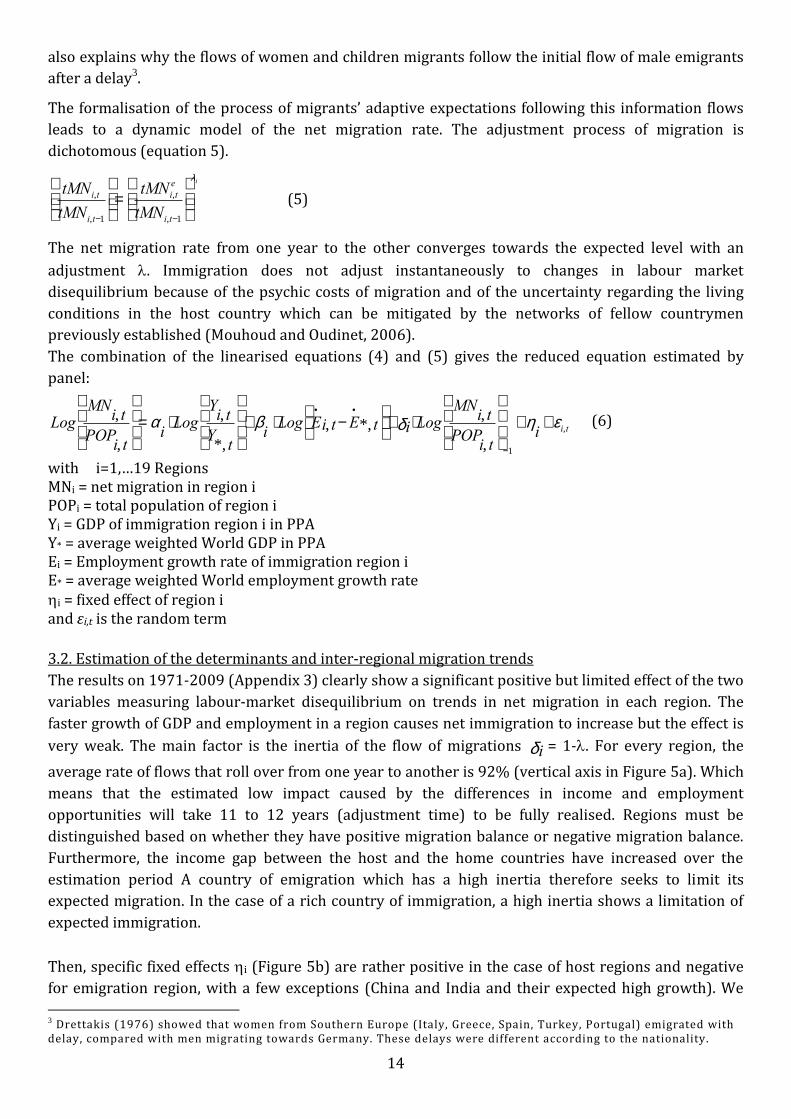
Table 1: National migration regimes Type of regions Y Employment
perspectives
Amenities (fixed
effects)
Specialization Demography (aging) Immigration policies
Regime A. « The core
skill replacement
migration regime «
Europe (West, UK and
North)
ODC (CAN NZ AUST)
USA
Y>Y*
Need for skilled labour in
manufacturing and in
knowledge-based
services; also for less
skilled labour in services
and housing sectors
Fixed effects
positive.
High level of
public-good
amenities
Both high skilled labour
intensive manufacturing
and services sectors
And low skilled labour
intensive in services
(public and private
services)
Aging population
Replacement
Selective policies favoring
skilled labour.
Restrictive policies
against unskilled labour,
especially from traditional
corridors (looking for
ethnical diversification)
Regime A'-Japan Y>Y*
Need for skilled
Employment in manuf.
And less skilled in
services and housing
sectors
Négative
amenities
High and low skilled
workers
Aging population
Replacement
Very restrictive
immigration policies
Regime B
“The mass labour
immigration and
replacement based
regime”
South Europe
East Asia High income
West Asia (Gulf
countries)
YY* Need for mass low skilled
migration in labour
intensive manufacturing,
construction, and service
sectors
Positive
amenities
Services, construction
and some high-tech
sectors
Temporary migration
Aging population, but less
than in A.
Replacement
Legalisation and mass
opening for South Europe.
Promoting temporal
migration
Regime C
China, India,
South America (Brazil),
CIS (Russia)
YY* Huge growth of labour
markets for skilled
labour
Positive
amenities for
China, India
(internal
migration)
Diversification No problem of aging
population.
Restrictive policies could
become more open in the
future
Internal migration as a
solution for mass labour
needs for China and India
+ skilled return migration
Regime D. Transit
countries, Climate-based
and forced south-south
migration.
Eastern Europe
West Asia (some)
Other South Asia
Africa
Central and South
America (some)
Y<Y* High skilled and low
skilled workers
Negative
amenities (in
particular transit
countries)
Natural resources and
labour intensive sectors
Demographic imbalances
with northern countries
Transit countries
Accepting refugees
Regime B of mass labour immigration and replacement includes the regions of Southern Europe,
Ireland and the high-income Gulf countries and East Asia countries. These regions are regions of mass
immigration. Any need adjustment in the labour market was met using immigration facilitated by
active immigration policies. These countries have done well to converge towards the countries of the
regime A, but the 2008 crisis has at least temporarily put an end to this convergence. Furthermore,
specialization of many of them is still concentrated in labour-intensive sectors in manufacturing,
construction, services and agriculture. The traditional immigration flows continue to come to these
countries in the sectors of construction, services, and consumer goods. Migrants accept the
geographical infra-national dispersion and some downgrading until they find a better match between
their qualifications and their jobs. The legalisation of irregular migrants by governments using lists of
workers provided by the employers encourages the kind of flexibility these countries require.
Downwards flexibility is also heavily used to soften the effects of the crisis.
In addition, these countries are experiencing an aging process that will result in an increasing need
for migrants. In that connection, one would also expect a change in migration trends based on stages
in demographic transitions. For example, migrants from Sub-Saharan African countries could replace
those from North Africa and the Middle East as the latter’s demographic transition is already more
advanced.

20
Countries that are part of regime B are catching up with developed countries as they have
requirements for their labour market due to a rapid and sustained growth. These countries have
opened up their immigration policies outside an aging population rationale.
Regime C as well includes emerging markets that are catching up with developed countries. But their
almost continental size and regional differences will here still allow adjustments by internal migration
for quite some time. This is obviously the case for China, India, and to a lesser degree South America.
For the regime D migration is largely linked to shocks of various kinds (ethnic conflicts, wars, natural
disasters, climate) that cause forced migration, mostly South-South and bordering countries. The
Libyan war, for example, is tantamount to a shock that could reverse the position on immigration in
North Africa and cause forced migration to the north of the Mediterranean. The rich countries' policies
towards refugees are then the fundamental variables of change in this type of migration. Some transit
countries, which are close to the target countries (Mexico towards USA, Eastern Europe towards West
Europe), see lesser-qualified migrants in sectors that are in need of labour. In these two regions,
labour migrations are more responsive to the conjuncture and have the most negative amenities.
4. Future scenarios
These six regional immigration regimes should change in the future based on growth trajectories and
changes in immigration policies. Tracing possible evolution scenarios for either, which we have drawn
from the AUGUR study of Europe in 2030, we have estimated migration patterns of the world’s
nineteen distinct regions based on three different scenarios (“reduced government”, “China and US
intervention” and “Multipolar Governance” in comparison to a “baseline scenario”), as presented in
section 4.1. With regards to the scenario “reduced government”, a more restrictive variant is
estimated “Eurozone breakup”. Policy choices pertaining to immigration and emigration are featured
within each scenario in section 4.2.
4.1. Endogenous migration scenarios
i) Baseline scenario
In this scenario of unbalanced and financialised development migration patterns depend on the
economic growth of regions, as determinant of their respective future labour-market needs, and on
network effects (see figures in Appendix 3). Regions belonging to the core skill replacement migration
regime (our Regime A) remain areas of immigration and even slightly increase their rates of
immigration. Japan initially closed to migration preserve a net migration balance on average around
zero, which should lead them to be even more hostile to migration. In contrast, immigration continues
to increase after the crisis in those regions of mass immigration Regime (like regions of Southern
Europe, Ireland and the high-income Gulf countries).
China and India become net immigration regions because of their high growth. In this scenario, these
two major countries would go from the C regime to a B regime from 2020 onwards. However, this
ignores the possibility for these huge, quasi-continental economies to adjust their labour market
needs through massive internal migration, thus delaying this shift. The model estimates potential
labour needs in the cities of both countries. These high needs are likely to be filled by internal
migration from rural areas rather than by international migration.

21
ii) « Reduced government » scenario
In this scenario the U.S. and European Union face pressure to reduce their debt and thus lower public
spending which in turn decreases employment and GDP. The effects of such policy choices on
immigration are clearly negative, but very weak due to the continuing role of network effects.
We thus project a decline in immigration in the regions of regime A, but this reduction is limited. For
example, net migration in West Europe (France and Germany) would decrease from 275 000 to 265
000. The effect is negative on employment and GDP. In 2030 the cumulative difference on the GDP is
about 3-4%, compared to the baseline scenario. Lower growth can be explained by lower level of
immigration, but the effect is limited. We find the results of studies regarding the positive impact of
immigration on the employment of host economies. Employment varies in the same way as does
immigration, so that at the macro level there is no impact on unemployment (Card, 1990; Hunt, 1992;
Greenwood and Hunt, 1995; Card, 2005; Mazier, Mouhoud, Oudinet, and Saglio, 2007). The variant
“Eurozone breakup” highlights, albeit in a limited way, this negative effect. The impact is stronger for
the countries of regime B in terms of mass immigration, but is still limited particularly on
employment.
In contrast, the exits decrease slightly all of which exacerbates frictions in the labour market and
increases poverty in regions of emigration. The consequence for the global economy overall is
negative.
iii) “China and US intervention” scenario
This scenario considers China’s stabilisation policies and US recovery. China gradually increases
government spending to 18% of GDP and gradually eliminates the external surplus and stabilises the
external position. West Europe reduces the current account surplus to zero to stimulate more growth
within Europe. Immigration is increasing everywhere except in Japan (regime A') which was already
in a situation of very low immigration. This effect is more important in Europe. The growth in
immigration from the baseline scenario is for example 40 000 in West Europe. But that effect is
marginal. In the United States the effect on immigration is also negligible. Symmetrically, countries of
emigration do not significantly change their number of emigrants.
iv) “Multipolar Governance” scenario
This scenario assumes regional cooperation is complemented by a level of global cooperation that
makes it possible for the world as a community to tackle common problems with regard to financial
imbalances, energy security and emissions and development of low-income countries.
Immigration increases slightly in the United States, the United Kingdom, and Southern Europe while
decreasing by 3% to 4% in other developed regions with declining growth. In West Europe,
immigration increases (+25000) but relatively less than in the China and US intervention scenario.
The emigration regions experience a relative decrease of exits, except China, which is becoming in the
long run an immigration country.

22
4.2. Scenarios of exogenous immigration and emigration policies
The goal now is to study how various immigration and emigration policies impact the above
scenarios. More specifically, we examine how proactive immigration policies may affect the baseline
scenario or the “China and US intervention » scenario. Conversely, the effects of the 'zero migration'
scenario will be estimated in the case of the “reduced government” and “China and US intervention”
scenarios (Table 2).
Table 2 : AUGUR Policy Scenarios
Migration Scenarios
Baseline Reduced
government China and US
intervention Multipolar
Governance
Constant migration X X
Zero migration X X X
Mass migration Replacement migration
X X
X
Climatic immigration Clim mig Clim mig + Clim mig stop
X X X
i) “Constant migration” scenario
In this scenario, the net migration rate of each region remains constant at the 2012 level, throughout
the period regardless of the macroeconomic evolution, assuming that immigration policies remain
unchanged and do not evolve according to the needs of the labour market. The impact is therefore
negative for those regions that have a projected growth in immigration and positive for the others but
the impact on the different regions’ growth is relatively marginal (Table 3).
Regions of the regime A should experience a negative, albeit negative evolution of their GDP and
employment, because they do not increase their rates of immigration as required by the needs of
labour markets. The impact in West and Northern Europe is just 0.25% on employment in 2030. It is
higher in the UK (-2.9%) and the United States (-1.5%). However, large areas of immigration (ODC)
have an employment growth (0.6%), since in the baseline scenario the initial high level of net
migration decreases slightly.
For regions of regime B of mass immigration (South Europe and West Asia), the effect of maintaining
constant migration rates on GDP and employment is also negative (-2.7% and -2.5%).
In the case of the dynamic emerging-market regions of regime C, maintaining the negative migration
balance of 2013 instead of fostering a positive evolution as required by the rates of economic growth
has a limited negative impact on employment (-3.8% for China and -0.6% for India). This is all the
more obvious as internal migration can easily replace the need for few millions immigrants.
For all other emigration countries of regime D the impact is still limited, although favorable to growth
and employment. The regions that gain the most in terms of jobs in this scenario are Central America
(+12%) and Other South Asia (+4.2%).
In the case of the “China and US intervention” scenario, we find the same changes than those in the
baseline.

23
Table 3: Constant migration scenario: IMPACT ON GDP AND EMPLOYMENT
CONSTANT MIGRATION
BASELINE CHINA AND US INTERVENTION
GDP Employment GDP Employment
2013 2030 2013 2030 2013 2030 2013 2030
USA 0.00 -0.24 0.00 -1.51 0.00 -0.21 0.00 -1.49
North Europe 0.00 -0.74 0.00 -3.85 0.00 -0.67 0.00 -3.81
South Europe 0.00 -0.03 0.00 -2.77 0.00 0.04 0.00 -2.92
West Europe 0.00 -0.12 0.00 -0.25 0.00 -0.03 0.00 -0.52
United Kingdom 0.00 -0.09 0.00 -2.88 0.00 -0.31 0.00 -3.14
East Europe 0.00 -0.14 0.00 3.82 0.00 0.02 0.00 3.50
China 0.00 -0.25 0.00 -3.80 0.00 0.00 0.00 -3.69
India 0.00 -0.12 0.00 -0.61 0.00 -0.05 0.00 -0.58
Other South Asia 0.00 0.18 0.00 4.20 0.00 0.23 0.00 4.07
Japan 0.00 -0.18 0.00 -0.79 0.00 -0.14 0.00 -0.78
Other Developed 0.00 0.10 0.00 0.67 0.00 0.16 0.00 0.72
West Asia 0.00 -0.46 0.00 -2.42 0.00 -0.34 0.00 -2.37
North Africa 0.00 0.26 0.00 3.13 0.00 0.30 0.00 2.84
Other Africa 0.00 0.00 0.00 0.91 0.00 0.10 0.00 1.03
East Asia High Income 0.00 0.27 0.00 3.40 0.00 0.34 0.00 3.38
Former Soviet Union 0.00 -0.07 0.00 0.45 0.00 0.06 0.00 0.63
South America 0.00 0.16 0.00 2.05 0.00 0.21 0.00 2.07
Central America 0.00 0.93 0.00 12.63 0.00 0.95 0.00 12.30
Other East Asia 0.00 0.04 0.00 1.37 0.00 0.10 0.00 1.36
Source: Authors’ calculation from CAM model simulations
ii) "Zero migration" scenario
In this scenario immigration policies try to cut off immigration flows.
The impact of a scenario of zero migration, implying a drastic reduction in labour and family
immigration, is simulated for global regions (Table 4). In this scenario of widespread protectionism
and cultural isolationism immigration policies are strongly enforced at regional levels (as exemplified
by the development of the Frontex agency for the EU’s Schengen area or construction of a wall on the
US-Mexico border). The great costs of border protection against migrants are not offset by the
expected benefits in labour markets.
For the regions of the regime A (ODC, United States, West Europe, United Kingdom, Northern Europe),
the impact is negative on employment. The regions of Europe are losing 4 to 14% of their jobs by
2030. West Europe, relatively less dependent on immigration than other parts of the regime A, should
see a more limited impact on employment (-4%). ODC countries lose twice as much as other regions
of the regime because of their greater dependence on immigration (employment decline of 14%).
For Japan (regime A'), which already has a closed policy, the impact is obviously negligible. However,
in the South of Europe (regime B), where we can find a greater dependency on more immigration, the
negative results are very significant, as highlighted by an estimated decrease in employment of 14%.

24
Table 4: Impact of “zero-migration” scenario on GDP and employment. ZERO MIGRATION
BASELINE CHINA AND US INTERVENTION
GDP Employment GDP Employment
2013 2030 2013 2030 2013 2030 2013 2030
USA 0.00 -1.71 0.00 -7.70 0.00 -1.80 0.00 -7.68
North Europe 0.00 -3.51 0.00 -13.56 0.00 -3.53 0.00 -13.54
South Europe 0.19 -0.48 0.05 -14.52 0.02 -0.38 0.01 -14.45
West Europe 0.01 -1.18 0.00 -4.00 0.00 -0.84 0.00 -4.14
United Kingdom 0.05 -1.19 0.01 -10.84 0.00 -1.89 0.00 -11.14
East Europe 0.05 -1.07 0.01 2.69 -0.01 -0.78 0.00 2.39
China 0.00 -0.71 0.00 -3.07 0.00 0.00 0.00 -2.92
India 0.00 -0.22 0.00 0.10 -0.01 -0.20 0.00 0.13
Other South Asia 0.00 0.46 0.00 8.72 -0.01 0.45 0.00 8.58
Japan 0.00 -0.30 0.00 -0.16 0.00 -0.39 0.00 -0.19
Other Developed 0.00 -3.86 0.00 -14.28 0.00 -3.88 0.00 -14.25
West Asia 0.00 -2.11 0.00 -8.34 0.00 -2.14 0.00 -8.29
North Africa 0.01 0.39 0.00 5.14 0.00 0.27 0.00 4.83
Other Africa 0.00 -0.13 0.00 1.75 0.00 0.00 0.00 1.88
East Asia High Income 0.02 -1.01 0.01 -3.99 0.01 -1.10 0.00 -4.04
Former Soviet Union 0.00 -0.26 0.00 1.18 0.00 -0.13 0.00 1.36
South America 0.00 0.36 0.00 3.92 0.00 0.39 0.00 3.94
Central America 0.00 1.15 0.00 17.25 0.00 1.05 0.00 16.88
Other East Asia 0.01 0.03 0.00 3.32 0.00 -0.05 0.00 3.30
Source : Authors’ calculation from CAM model simulations MIGRATION ZERO
REDUCED GOVERNMENT EUROZONE BREAKUP
GDP Employment GDP Employment
2013 2030 2013 2030 2013 2030 2013 2030
USA 0.00 -1.26 0.00 -7.50 0.00 -1.27 0.00 -7.49
North Europe -0.01 -3.17 0.00 -13.53 -0.03 -3.17 -0.01 -13.47
South Europe 0.19 -0.37 0.05 -14.48 0.03 -0.20 0.01 -14.55
West Europe 0.03 -1.02 0.01 -3.94 0.01 -1.01 0.00 -3.87
United Kingdom 0.05 -0.66 0.01 -10.68 0.01 -1.92 0.00 -11.01
East Europe 0.06 -1.13 0.01 2.98 0.00 -0.35 0.00 2.65
China 0.00 -0.57 0.00 -3.03 -0.01 -0.59 0.00 -3.03
India 0.00 -0.28 0.00 -0.10 -0.01 -0.29 0.00 -0.09
Other South Asia 0.00 0.54 0.00 9.02 -0.01 0.52 0.00 9.03
Japan 0.00 -0.24 0.00 -0.14 0.00 -0.25 0.00 -0.14
Other Developed 0.00 -3.25 0.00 -14.15 0.00 -3.26 0.00 -14.14
West Asia 0.00 -2.07 0.00 -8.35 0.00 -2.08 0.00 -8.34
North Africa 0.01 0.51 0.00 5.17 0.00 0.49 0.00 5.19
Other Africa 0.00 -0.02 0.00 1.60 0.00 -0.03 0.00 1.62
East Asia High Income 0.02 -0.94 0.01 -3.98 0.01 -0.95 0.00 -3.98
Former Soviet Union 0.00 -0.20 0.00 1.23 0.00 -0.21 0.00 1.23
South America 0.00 0.31 0.00 3.63 0.00 0.30 0.00 3.65
Central America 0.00 1.30 0.00 17.95 0.00 1.29 0.00 17.95
Other East Asia 0.01 0.13 0.00 3.46 0.00 0.11 0.00 3.47
Source : Authors’ calculation from CAM model simulations

25
The negative impact is significant in West Asia (-8%) and more limited in East Asia HI (-4%).
The regions of origin of the regime C gain in this process, but the effects are negligible for India whose
net migration balances remain minor. The effect is negative for China (-3%) but positive for Russia
(+1.2%), and South America (+3.9%). Among the regions of the regime D, those who gain the most are
the countries of Central America. Other regions have mostly no changes in jobs.
The effect of a zero immigration policy in alternative scenarios (“reduced government” and “Eurozone
breakup”, “China and US intervention”, “Multipolar Governance”) displays similar effects as in the case
of the baseline scenario.
The results clearly show a negative effect of the zero-immigration scenario for the global economy.
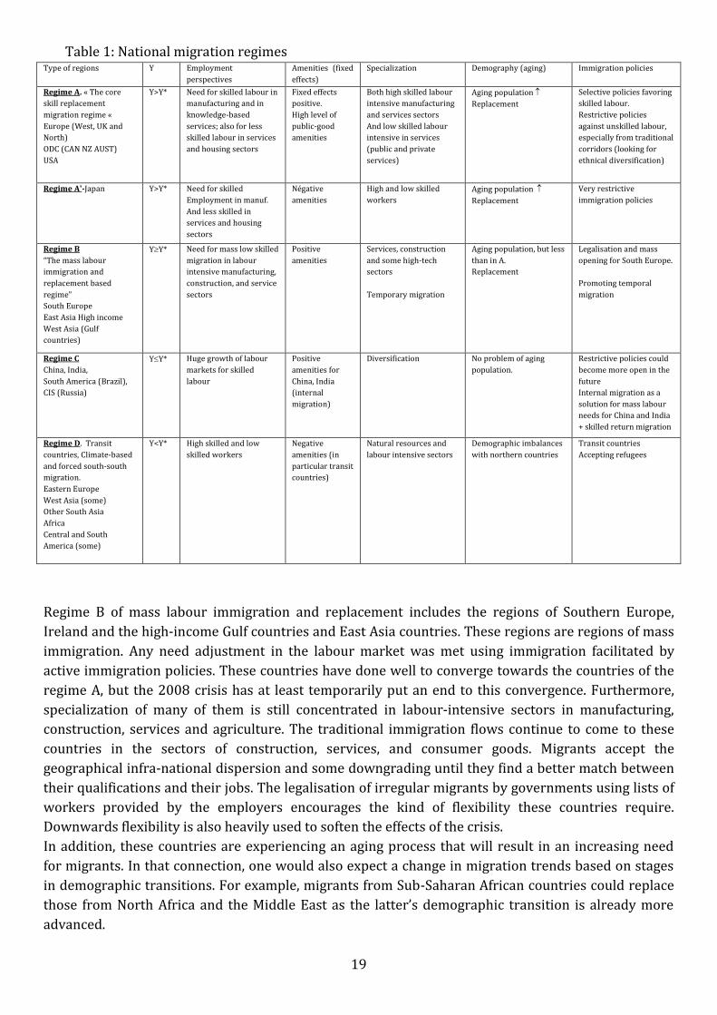
iii) “Mass migration” scenario
A scenario of "mass migration,” doubling the rates of migration, has significant positive effects on
growth, given the shortage of skilled labour and the important needs of human resources in services.
Labour markets easily find the human resources they need which in turn fuels growth. The problems
of aging in the developed economies get solved more easily with an increase in both personal and
health services, using both the skilled and unskilled labour provided by this mass immigration.
Congestion problems can be solved by an extensive policy of housing construction facilitated by the
mass of immigrant labour.
The doubling of flows does not have a great impact at the macro-economic level, since the starting
level is rather low. Employment in the developed countries of regime A increases between 4 and 14%,
and GDP between 0.7% and 3.8%. The impact is higher for regime B countries. Southern Europe sees
its employment levels grow by 14.5% and the growth for West Asia is 8.3%.
Among the regions of emigration, regimes C (without China) and D, Central America and North Africa
are most affected by this doubling of flows because of their respective proximity to the United States
and Europe. The impact on employment is negative in both regions (-17.3% for Central America and -
5.1% for North Africa)..
If the mass-migration shock occurs within the "Multipolar Governance" scenario, the results are
similar.
26
Table 5: Impact of migration doubled scenario GDP and employment. MIGRATION DOUBLED
BASELINE MULTIPOLAR GOVERNANCE
GDP Employment GDP Employment
2013 2030 2013 2030 2013 2030 2013 2030
USA 0.00 1.71 0.00 7.70 0.00 1.59 0.00 7.56
North Europe 0.00 3.49 0.00 13.62 0.00 0.35 0.00 12.66
South Europe -0.19 0.51 -0.05 14.50 -0.08 0.25 -0.02 14.36
West Europe -0.01 1.18 0.00 4.01 -0.01 0.46 0.00 3.88
United Kingdom -0.05 0.70 -0.01 10.71 -0.01 0.32 0.00 10.64
East Europe -0.05 1.08 -0.01 -2.70 -0.01 0.66 0.00 -2.20
China 0.00 0.71 0.00 3.07 0.00 0.00 0.00 2.85
India 0.00 0.21 0.00 -0.10 0.00 0.06 0.00 -0.06
Other South Asia 0.00 -0.48 0.00 -8.72 0.01 0.29 0.00 -8.90
Japan 0.00 0.30 0.00 0.16 0.00 0.21 0.00 0.15
Other Developed 0.00 3.86 0.00 14.31 0.00 3.68 0.00 14.21
West Asia 0.00 2.11 0.00 8.34 0.00 1.78 0.00 8.21
North Africa -0.01 -0.41 0.00 -5.14 0.00 0.20 0.00 -4.82
Other Africa 0.00 0.12 0.00 -1.75 0.00 0.10 0.00 -1.43
East Asia High Income -0.02 1.01 -0.01 3.99 -0.01 0.11 0.00 3.65
Former Soviet Union 0.00 0.25 0.00 -1.18 0.00 -0.04 0.00 -1.63
South America 0.00 -0.37 0.00 -3.92 0.00 0.05 0.00 -3.75
Central America 0.00 -1.18 0.00 -17.31 0.00 -1.17 0.00 -18.23
Other East Asia -0.01 -0.03 0.00 -3.32 0.00 0.21 0.00 -3.34
Source: Authors’ calculation from CAM model simulations
iv) « Replacement migration » scenario
Immigration in this scenario can stabilise the dependency ratio (inactive / population of working age)
in those regions where the rate increases at the 2030 horizon namely: Europe (5 blocks), High Income
East Asia, Former Soviet Union, China, Japan, United States and Other Developed countries. To
stabilise its ratio, West Europe and the United States require an increase of immigrants equivalent to
2 and a half million workers. For China, more than 6 million people are needed to prevent the
dependency ratio to increase. The strong need for labour is met by emigration from Africa, Latin
America and East Asia with low incomes.
As in previous shocks of mass immigration, immigration has a positive effect on activity. Employment
grows strongly in the countries of East Asia with high incomes (30% by 2030), in West Europe
(+25%), and in the United States (+19%). Similarly, the loss in labour reduces employment by 45% in
Central America, 27% in South Asia and 16% in North Africa.

27
Table 6 : Impact of the replacement migration scenario on employment. REPLACEMENT MIGRATION
Net migration baseline
Net migration with constant dependance
ratio
Variation with baseline
Impact on Employment
2013 2030 2013 2030 2013 2030 2013 2030
USA 0.91 1.27 3.31 3.85 2.40 2.58 0.00 19.10
North Europe 0.11 0.19 0.35 0.23 0.24 0.04 0.00 10.97
South Europe 0.73 1.04 1.51 1.68 0.78 0.65 -0.10 6.97
West Europe 0.27 0.28 1.33 2.87 1.06 2.59 -0.01 25.57
United Kingdom 0.22 0.39 0.66 0.75 0.44 0.36 -0.03 11.85
East Europe 0.02 -0.35 0.98 0.23 0.96 0.58 -0.03 28.51
China -0.39 7.27 -1.23 14.18 -0.84 6.92 0.00 13.72
India -0.43 0.61 -1.65 0.58 -1.22 -0.04 0.00 -1.40
Other South Asia -1.00 -3.76 -3.81 -8.56 -2.81 -4.80 0.00 -26.77
Japan -0.02 0.01 2.14 0.48 2.16 0.47 -0.01 23.27
Other Developed 0.46 0.46 0.98 1.04 0.51 0.59 0.00 21.65
West Asia 1.04 1.81 1.04 1.81 0.00 0.00 0.00 0.17
North Africa -0.22 -1.28 -0.85 -3.17 -0.63 -1.89 0.00 -16.19
Other Africa -0.38 -1.46 -1.46 -3.99 -1.08 -2.53 0.00 -6.14
East Asia High Income 0.21 0.09 0.11 1.51 -0.10 1.41 0.00 30.66
Former Soviet Union -0.09 -0.19 2.07 0.58 2.16 0.77 0.00 20.66
South America -0.35 -1.51 -1.34 -3.82 -0.99 -2.32 0.00 -12.86
Central America -0.49 -2.97 -1.87 -5.40 -1.38 -2.44 0.00 -45.02
Other East Asia -0.59 -1.89 -2.26 -4.84 -1.67 -2.94 0.00 -11.22
v) “Climatic shocks” scenarios
Finally, we consider a nightmare scenario whereby climate change triggers large South - South flows
of refugees, which may still spill over into northern areas. 80% of climatic refugees would go to
neighbouring countries in the South. Opportunities to migrate to the north may open up in the case of
a more open scenario, notably the “mass-migration” scenario considered above. On other hand, the
North would obviously refuse to take in climate migrants if it opts for the zero migration scenario. The
impoverishment of the South in the face of climate shocks would have a negligible impact on global
growth, but would increase inequalities.
The shock of environmental immigration is analysed using three additional scenarios:
-The “Clim mig" looks at the effect on net migration of a natural disaster. A decline in private
investment and public spending by 10 percentage points of GDP is simulated in five areas that are
most likely to experience a climate disaster: North Africa and Sub-Saharan Africa, South Asia, low-
income East Asia, and Central America.
-In the "Clim mig+" climate shock, we see a tenfold increase in the income elasticity relative to the
initial climatic choc. Migrants become more sensitive to the sharp fall in their income.
-Lastly, in the variant "clim mig stop", following the initial shock, developed countries adopt a
restrictive immigration policy by closing their borders (constant migration as of 2013)

28
Table 7: Scenario climatic migration: decline in private investment and public spending by 10
percentage points of GDP in five regions: North Africa and Sub-Saharan Africa, South Asia and low-
income East and Central America CLIMATIC MIGRATION
CLIM MIG CLIM MIG + CLIM MIG STOP
GDP Employment GDP Employment GDP Employment
2013 2030 2013 2030 2013 2030 2013 2030 2013 2030 2013 2030
USA -0.47 -1.49 -0.17 0.16 -0.48 1.37 -0.17 18.15 -0.47 -1.67 -0.17 -1.18
North Europe -0.87 -1.84 -0.25 -0.05 -0.87 2.80 -0.25 24.80 -0.87 -2.42 -0.25 -3.55
South Europe -3.48 -4.22 -0.88 -0.87 -3.53 -3.11 -0.90 8.04 -3.48 -4.20 -0.88 -3.23
West Europe -1.17 -3.23 -0.34 -0.47 -1.17 -0.59 -0.34 14.32 -1.17 -3.28 -0.34 -0.67
United Kingdom -1.70 -4.19 -0.49 -0.75 -1.71 -3.30 -0.49 17.76 -1.70 -4.18 -0.49 -3.30
East Europe -2.20 -4.46 -0.31 -0.36 -2.22 -2.62 -0.31 3.28 -2.20 -4.51 -0.31 -0.20
China -1.82 -4.13 -0.11 -0.04 -1.81 -3.23 -0.11 0.84 -1.82 -4.15 -0.11 -0.04
India -0.83 -1.67 -0.03 0.18 -0.83 -1.88 -0.03 -6.20 -0.83 -1.68 -0.03 0.19
Other South Asia -15.62 -27.60 -0.41 -1.00 -15.62 -27.40 -0.41 -4.13 -15.62 -27.59 -0.41 -0.54
Japan -0.81 -2.45 -0.26 -0.36 -0.81 -0.85 -0.26 6.15 -0.81 -2.46 -0.26 -0.36
Other Developed -0.41 -1.09 -0.12 0.27 -0.41 1.53 -0.12 11.57 -0.41 -1.00 -0.12 0.69
West Asia -0.82 -1.81 -0.10 0.19 -0.82 -0.79 -0.10 2.96 -0.82 -1.82 -0.10 0.19
North Africa -16.88 -24.44 -0.99 -1.32 -16.88 -24.32 -0.99 -3.62 -16.88 -24.42 -0.99 -1.02
Other Africa -16.07 -21.46 -0.37 -1.11 -16.07 -21.78 -0.37 -8.73 -16.07 -21.46 -0.37 -0.99
East Asia High Income -2.26 -3.80 -0.65 -0.60 -2.27 -2.41 -0.65 7.51 -2.26 -3.58 -0.65 1.92
Former Soviet Union -0.55 -0.88 -0.06 0.49 -0.55 0.14 -0.06 3.83 -0.55 -0.88 -0.06 0.55
South America -0.32 -0.96 -0.04 0.52 -0.32 -0.24 -0.04 3.52 -0.32 -0.94 -0.04 0.71
Central America -15.71 -22.01 -2.19 -2.43 -15.71 -20.83 -2.19 8.83 -15.71 -21.98 -2.19 -1.58
Other East Asia -16.47 -23.00 -0.79 -1.24 -16.47 -22.71 -0.79 -3.33 -16.47 -22.99 -0.79 -1.05
Source : Authors’ calculations from CAM model simulations
In the five regions affected by natural disasters, the GDP initially falls by about 15% the year of the
shock and more than 20% by 2030 in all three variants studied (clim mig, clim mig+ and Clim mig
stop). For developed countries, the GDP is less affected in the variant “clim mig+” than in the variants
“clim mig” and “clim mig stop”. As migration is more sensitive to income differentials in the scenario
“clim mig +”, migration flows will increase (table 8) to the USA (+4,7 millions), West Europe (1.7
million), the United Kingdom (1.12 million) and China (3.987 million) increasing the influx of workers
and stimulating thereby the DGP. The variant “clim mig stop” is more costly in terms of employment in
developed countries in view of their restrictive policy on immigration.

29
Table 8: Scenario climatic migration: decline in private investment and public spending by 10
percentage points of GDP in five regions: North Africa and Sub-Saharan Africa, South Asia and East
low-income and Central America CLIMATIC MIGRATION
NET MIGRATION VARIATION WITH BASELINE
BASELINE CLIM MIG CLIM MIG + CLIM MIG STOP CLIM MIG CLIM MIG + CLIM MIG STOP
2013 2030 2013 2030 2013 2030 2013 2030 2013 2030 2013 2030 2013 2030
USA 0.91 1.27 0.91 1.28 1.26 5.97 0.91 0.91 0.00 0.01 0.35 4.70 0.00 -0.36
North Europe 0.11 0.19 0.11 0.19 0.13 0.80 0.11 0.11 0.00 0.00 0.02 0.61 0.00 -0.08
South Europe 0.73 1.04 0.73 1.03 0.82 1.94 0.73 0.73 0.00 0.00 0.08 0.91 0.00 -0.30
West Europe 0.27 0.28 0.27 0.28 0.43 1.98 0.27 0.27 0.00 0.00 0.16 1.70 0.00 -0.01
United Kingdom 0.22 0.39 0.22 0.39 0.28 1.51 0.22 0.22 0.00 0.00 0.05 1.12 0.00 -0.16
East Europe 0.02 -0.35 0.02 -0.31 0.06 -0.01 0.02 -0.29 0.00 0.04 0.03 0.33 0.00 0.05
China -0.39 7.27 -0.39 7.35 -0.36 11.14 -0.39 7.35 0.01 0.08 0.03 3.87 0.00 0.08
India -0.43 0.61 -0.42 0.69 -0.94 -8.84 -0.42 0.69 0.01 0.08 -0.51 -9.45 0.01 0.08
Other South Asia -1.00 -3.76 -0.99 -3.76 -1.07 -4.97 -1.00 -3.54 0.01 0.00 -0.06 -1.20 0.01 0.23
Japan -0.02 0.01 -0.02 0.01 0.09 0.28 -0.02 0.01 0.00 0.00 0.10 0.28 0.00 0.00
Other Developed 0.46 0.46 0.46 0.46 0.53 1.00 0.46 0.46 0.00 0.00 0.06 0.54 0.00 0.01
West Asia 1.04 1.81 1.04 1.83 1.08 2.76 1.04 1.83 0.00 0.02 0.04 0.94 0.00 0.02
North Africa -0.22 -1.28 -0.23 -1.33 -0.25 -1.80 -0.23 -1.25 0.00 -0.05 -0.03 -0.52 0.00 0.03
Other Africa -0.38 -1.46 -0.39 -1.93 -0.99 -8.96 -0.39 -1.81 -0.01 -0.48 -0.61 -7.50 -0.01 -0.36
East Asia High Income 0.21 0.09 0.21 0.09 0.28 0.41 0.21 0.21 0.00 0.00 0.07 0.32 0.00 0.12
Former Soviet Union -0.09 -0.19 -0.09 -0.14 -0.04 0.63 -0.09 -0.13 0.00 0.05 0.05 0.82 0.00 0.06
South America -0.35 -1.51 -0.35 -1.30 -0.22 -0.06 -0.35 -1.22 0.01 0.20 0.13 1.45 0.01 0.28
Central America -0.49 -2.97 -0.49 -2.73 -0.34 -0.57 -0.50 -2.58 0.00 0.24 0.15 2.40 0.00 0.39
Other East Asia -0.59 -1.89 -0.60 -2.09 -0.71 -3.22 -0.60 -1.96 -0.01 -0.20 -0.12 -1.33 -0.01 -0.07
Source : Authors’ calculations from CAM model simulations
Conclusion
From specific estimations, we define four immigration regimes have been build that cut across the
major regions of the model : The “core skill replacement migration regime” based on selective
policies using migration to fill high-skilled labour needs (United Kingdom, West and Northern Europe,
Canada, Australia, and United States), “mass immigration and replacement" applies to South Europe,
East Asia High Income, and part of West Asia (Gulf countries), "big fast-growing emerging regions of
future mass immigration,” notably China, India and “South-South migration” based forced migration
much of it by climate change, which may likely occur in South Asia, part of West Asia, and, most of
Africa (without South Africa). Migrations in transit countries (Central America to USA, and East
Europe to UK and West Europe) are based on low skilled migrants in labour-intensive sectors.
The different scenarios of governance don’t change dramatically the evolution of the migration
dynamic between regions until 2030. Nonetheless, there is a main interesting change for two large
countries of emigration (regime C), China and India, which are about to become net immigration
regions (regime B) because of their huge needs of labour according to their high GDP growth rates.
But these needs are also likely to be filled by internal migration from rural areas rather than by
international migration. Regions of the Regime A remain areas of immigration and even slightly
increase their rates of immigration and those of emigration (Regime D) remains also large regions of
emigration. The mass migration regions (regime B) continue to increase their immigration rate.

30
Paradoxically, in the case of the “reduced government scenario”, the regions of the so-called
developed countries most durably affected by the crisis (regime A and B) are also those that have
ageing population and which are in high need of skilled and unskilled labour.
The tendencies to follow the depressive effects of the global crisis are reflected in immigration and
open trade policies that are very restrictive or highly selective in favour of the skilled. These choices
of migration policies reinforce the deflationary process resulting in reduced opportunities for
renewed growth in industrial areas and are not offset by the dynamism of growth in emerging
countries.
The crisis and its aggravation thus clearly favour scenarios of immigration policy along the “zero
migration” or “constant migration”. Paradoxically, the zones most durably affected by the crisis
(immigration regime A and B of the So-called developed countries) are also those that have ageing
population and which are in high need of skilled and unskilled labour. Ageing populations are also
those where public opinion shows an aversion to migration the same way the very least qualified and
most vulnerable vis a vis globalisation are those showing support for open policies.
Three options are possible: one going along the depressive process by espousing restrictive
immigration policies that remain expensive. The second involves a highly selective immigration
policy. The immigration policy changes clearly in favour of a policy of selective entry according to
labour market needs, which is revised annually. Under these conditions the demographic revival
already appearing would be reinforced by a rejuvenation of the population brought about by a more
open immigration policy. Political and institutional factors play a fundamental role in the emergence
of this optimistic assumption. The rise of isolationism in Europe and the ghettoisation of suburban
areas can hinder the application of such a policy of openness to migration. However, the continued
entry of qualified persons through the implanting of students in particular is capable of contributing
to the rejuvenation of the European population.
The third scenario, the mass migration scenario, allows letting go of the growth related constraints
and get out of the deflationist spiral. This pro-active approach could cause public opinions to change
in line with public interest. This scenario of mass migration has more of a chance to see the light
under a growth hypothesis. However, and as noted above, restrictive policies weaken the prospects of
sustainable recovery causing a vicious cycle that can only be broken by pro-active policies or by
irresistible shocks, such as climatic shocks, affecting regions A and B.
References
Beine M., Defoort C. and Docquier F. (2011) « A panel data analysis of the Brain Gain » World
Development, April, 2011, Vol. 39, No. 4.
Card D. (1990) « The Impact of the Mariel Boatlift on the Miami Labor Market », Industrial and Labor
Relations Review, n° 43, pp. 245-257.
Card D (2005) “Is the new immigration really so bad?”, Economic Journal, 115, November.
Drettakis EG (1976) Distributed lags models for the quaterly migration flows of West Germany,
Journal of the Royal Statistical Society, 139, pp 365-373.
Graves PE. (1980) Migration and Climate, Journal of Regional Science, 20, pp 227-237.
31
Greenwood MJ (1985) Human migration, theory, models and empirical studies, Journal of Regional
Science, 25, pp 521-544.
Greenwood MJ, Hunt GL (1995) “Economic Effects of Immigrants on Native and Foreign-born
Workers : complementarity, substitutability and other Channel of Influence”, Southern Economic
Journal, 61, pp 1076-1097.
Harris J., Todaro M. (1970). Migration, Unemployment & Development: A Two-Sector Analysis.
American Economic Review, March 1970, 60(1), pp 26-42.
Hunt J. (1992) “The impact of the 1962 Repatriates from Algeria on the French Labor Market”,
Industrial and Labor Relations Review, Vol. 45, No. 3, pp. 556-572.
Marfouk A. (2007) “Brain Drain in Developing Countries”, World Bank Economic Review, Oxford
University Press, vol. 21(2), Jun, pp 193-218.
Mazier J., Mouhoud EM., Oudinet J., and Saglio S. (2007) Quel rôle jouent les migrations dans le
fonctionnement de l’Union Monétaire ?, in “L’Europe et ses migrants. Ouverture ou repli », MOUHOUD
EM, OUDINET J. (eds), L’Harmattan, pp 151-214.
Mouhoud EM, Oudinet J. (2006) « Migrations et marché du travail dans l’espace européen »,
Economie Internationale, La revue du CEPII, La Documentation Française, n°105, 1er trimestre, pp 7-
39.
Mouhoud EM, Oudinet J. (2010) Inequality and Migration: What different European patterns of
migration tell us, International Review of Applied Economics, vol 24, N°3, July 2010, pp 407-426.
OECD (2009) International Migration Outlook, SOPEMI.
OECD (2010) International Migration Outlook, SOPEMI.
Ratha, Dilip K., Shaw W. (2006). South-South Migration and Remittances , Development
Prospects Group, World Bank. http://go.worldbank.org/U4RXL56V20
Saint-Paul, G. (1997) “Economic integration, factor mobility and wage convergence”, International
Tax and Public Finance, Volume 4, Number 3, 291-306.
Stark O, Bloom DE (1985) “The new economics of Labor Migration”, American Economic Review, 75,
pp173-178.

32
APPENDICES
Appendix 1: The 19 regions or areas of the CAM model
CAM : Demand Model with 4002 equations (66 behavioral equations estimated in pool and thus 66
instruments for shock simulation)
EUN (North Europe) : Denmark, Finland, Norway, Sweden
EUW (West Europe) : Austria, Belgium, Luxembourg, Switzerland, Germany, France, Netherlands
UK : United Kingdom
EUS (South Europe) : Spain, Greece, Ireland, Italy, Portugal, Other Europe
EUE (East Europe) : Albania, Bulgaria, Former Czechoslovakia, Hungary, Poland, Romania, Former
Yugoslavia
US (USA) : United states
JA (Japan) : Japan
OD (Other Developed) : Australia, Canada, Israel, New Zealand
EAH (East Asia High Income) : Hong-Kong SAR of China, Republic of Korea, Singapore, Taiwan
CI (CIS) : Former Soviet Union countries
WA (West Asia) : United Arab Emirates, Bahrain, Iraq, Iran, Jordan, Kuwait, Lebanon, Oman, Saudi
Arabia, Syrian Arab Republic, Turkey, Republic of Yemen , Other middle east
AM (South America) : Argentina, Bolivia, Brazil, Chile, Columbia, Ecuador, Peru, Paraguay, Uruguay,
Venezuela
ACX (Central America) : Costa Rica, Cuba, Dominican Republic, Guatemala, Honduras, Haiti, Jamaica,
Mexico, Nicaragua, Panama, El Salvador, Other America
CN (China) : China inc Macao
EAO (Other East Asia) : Indonesia, Cambodia, Republic of Korea, Lao Republic, Myanmar, Mongolia,
Malaysia, Papua New Guinea, Philippines, Thailand, Vietnam, Other Oceania
IN (India) : India
ASO (Other South Asia) : Afghanistan, Bangladesh, Sri Lanka, Nepal, Pakistan, Other South Asia
AFN (North Africa) : Algeria, Egypt, Libyan Arab Jamahiriya, Morocco, Sudan, Tunisia
AFS (Other Africa) : Africa small LDCs, Angola , Burkina Faso, Burundi, Benin, Democratic Republic of
the Congo, Central African Republic, Congo, Cote d'Ivoire, Cameroon, Ethiopia, Ghana, Guinea, Kenya,
Liberia, Madagascar, Mali, Mauritania, Malawi, Mozambique, Niger, Nigeria, Rwanda, Sierra Leone,
Senegal, Somalia, Chad, Togo, United Republic Of Tanzania, Uganda, South Africa, Zambia, Zimbabwe,
Other Africa

33
Figures A2: rate of high-skilled expatriates of the main areas affected by the brain drain (compared to
the expatriate population +)
0.00%
5.00%
10.00%
15.00%
1975 1980 1985 1990 1995 2000
North Africa
0.00%
5.00%
10.00%
15.00%
1975 1980 1985 1990 1995 2000
Other Africa
0.00%
20.00%
40.00%
1975 1980 1985 1990 1995 2000
Central America

34
APPENDIX 3 : Equation net migration rate. Dependent Variable: (LOG(1 +NIMU_?/N_?))
Method: Pooled EGLS (Cross-section SUR)
Date: 10/27/11 Time: 17:59
Sample (adjusted): 1971 2009
Included observations: 39 after adjustments
Cross-sections included: 19
Total pool (balanced) observations: 741
Linear estimation after one-step weighting matrix Variable Coefficient Std. Error t-Statistic C 1.59E-05 6.14E-06 2.590957
LOG(YR_?) 8.03E-05 7.42E-06 10.81859
LOG(1+D(LOG(NE_?))-D(LOG(NE_W_0))) 0.001435 0.000112 12.86799
EUN--(LOG(1+NIMU_EUN(-1)/N_EUN(-1))) 1.011922 0.019947 50.72955
EUW--(LOG(1+NIMU_EUW(-1)/N_EUW(-1))) 0.937669 0.008868 105.7413
EUK--(LOG(1+NIMU_EUK(-1)/N_EUK(-1))) 1.013696 0.007574 133.8383
EUS--(LOG(1+NIMU_EUS(-1)/N_EUS(-1))) 0.983044 0.008205 119.8096
EUE--(LOG(1+NIMU_EUE(-1)/N_EUE(-1))) 0.851074 0.020275 41.97575
US--(LOG(1+NIMU_US(-1)/N_US(-1))) 0.941910 0.007810 120.6083
JA--(LOG(1+NIMU_JA(-1)/N_JA(-1))) 0.694097 0.016993 40.84556
OD--(LOG(1+NIMU_OD(-1)/N_OD(-1))) 0.867329 0.014182 61.15655
EAH--(LOG(1+NIMU_EAH(-1)/N_EAH(-1))) 0.790473 0.012356 63.97502
CI--(LOG(1+NIMU_CI(-1)/N_CI(-1))) 0.922998 0.006002 153.7874
WA--(LOG(1+NIMU_WA(-1)/N_WA(-1))) 0.979294 0.007580 129.1880
AMS--(LOG(1+NIMU_AMS(-1)/N_AMS(-1))) 0.942100 0.014730 63.95801
ACX--(LOG(1+NIMU_ACX(-1)/N_ACX(-1))) 0.753737 0.022134 34.05303
CN--(LOG(1+NIMU_CN(-1)/N_CN(-1))) 1.112677 0.043741 25.43759
EAO--(LOG(1+NIMU_EAO(-1)/N_EAO(-1))) 0.927683 0.011040 84.02549
IN--(LOG(1+NIMU_IN(-1)/N_IN(-1))) 1.005318 0.011359 88.50130
ASO--(LOG(1+NIMU_ASO(-1)/N_ASO(-1))) 0.936680 0.008398 111.5343
AFN--(LOG(1+NIMU_AFN(-1)/N_AFN(-1))) 0.948540 0.013282 71.41415
AFS--(LOG(1+NIMU_AFS(-1)/N_AFS(-1))) 0.937856 0.009673 96.95729
Fixed Effects (Cross)
EUN--C -1.86E-05
EUW--C 1.32E-05
EUK--C -2.53E-05
EUS--C 0.000153
EUE--C -0.000145
US--C 9.93E-05
JA--C -4.97E-05
OD--C 0.000614
EAH--C 0.000145
CI--C -3.66E-05
WA--C 9.66E-05
AMS--C -7.99E-05
ACX--C -0.001014
CN--C 0.000128
EAO--C -2.65E-06
IN--C 9.38E-05
ASO--C -1.19E-05
AFN--C -2.20E-05
AFS--C 6.18E-05 Effects Specification Cross-section fixed (dummy variables)

35
SCENARIO BASE LINE : Estimated net migration balance, Author’s Projections to 2030 from CAM Model
.00
.02
.04
.06
.08
.10
.12
.14
70 75 80 85 90 95 00 05 10 15 20 25 30
North Europe
-0.2
0.0
0.2
0.4
0.6
0.8
1.0
1.2
1.4
70 75 80 85 90 95 00 05 10 15 20 25 30
South Europe
-0.2
0.0
0.2
0.4
0.6
0.8
1.0
70 75 80 85 90 95 00 05 10 15 20 25 30
West Europe
-.04
.00
.04
.08
.12
.16
.20
.24
70 75 80 85 90 95 00 05 10 15 20 25 30
United Kingdom
-.5
-.4
-.3
-.2
-.1
.0
.1
70 75 80 85 90 95 00 05 10 15 20 25 30
East Europe
-0.4
0.0
0.4
0.8
1.2
1.6
2.0
70 75 80 85 90 95 00 05 10 15 20 25 30
West Asia
-1.0
-0.8
-0.6
-0.4
-0.2
0.0
0.2
70 75 80 85 90 95 00 05 10 15 20 25 30
North Africa
-1.0
-0.8
-0.6
-0.4
-0.2
0.0
0.2
70 75 80 85 90 95 00 05 10 15 20 25 30
Other Africa
-.2
-.1
.0
.1
.2
.3
70 75 80 85 90 95 00 05 10 15 20 25 30
East Asia High Income
-1.4
-1.2
-1.0
-0.8
-0.6
-0.4
-0.2
0.0
0.2
70 75 80 85 90 95 00 05 10 15 20 25 30
Other East Asia
-2.8
-2.4
-2.0
-1.6
-1.2
-0.8
-0.4
0.0
0.4
70 75 80 85 90 95 00 05 10 15 20 25 30
Other South Asia
-.4
-.3
-.2
-.1
.0
.1
.2
70 75 80 85 90 95 00 05 10 15 20 25 30
Former Soviet Union
-0.8
-0.4
0.0
0.4
0.8
1.2
1.6
2.0
2.4
2.8
3.2
70 75 80 85 90 95 00 05 10 15 20 25 30
China
-.8
-.6
-.4
-.2
.0
.2
.4
.6
.8
70 75 80 85 90 95 00 05 10 15 20 25 30
India
-.2
-.1
.0
.1
.2
.3
70 75 80 85 90 95 00 05 10 15 20 25 30
Japan
-1.2
-1.0
-0.8
-0.6
-0.4
-0.2
0.0
0.2
70 75 80 85 90 95 00 05 10 15 20 25 30
South America
-2.4
-2.0
-1.6
-1.2
-0.8
-0.4
0.0
70 75 80 85 90 95 00 05 10 15 20 25 30
Central America
0.2
0.4
0.6
0.8
1.0
1.2
1.4
1.6
1.8
2.0
70 75 80 85 90 95 00 05 10 15 20 25 30
USA
.0
.1
.2
.3
.4
.5
.6
70 75 80 85 90 95 00 05 10 15 20 25 30
Other Developed

36