Embed Size (px)
Citation preview

109
Bulletin of the Seismological Society of America, Vol. 95, No. 1, pp. 109–134, February 2005, doi: 10.1785/0120030166
Off-Fault Secondary Failure Induced by a Dynamic Slip Pulse
by James R. Rice, Charles G. Sammis, and Robert Parsons*
Abstract We develop a 2D slip-weakening description of a self-healing slip pulsethat propagates dynamically in a steady-state configuration. The model is used toestimate patterns of off-fault secondary failure induced by the rupture, and also toinfer fracture energies G for large earthquakes. This extends an analysis for a semi-infinite rupture (Poliakov et al., 2002) to the case of a finite slipping zone length Lof the pulse. The dynamic stress drop, when divided by the drop from peak to residualstrength, determines the ratio of L to the slip-weakening zone length R. Predictedoff-fault damage is controlled by that scaled stress drop, static and dynamic frictioncoefficients, rupture velocity, principal prestress orientation, and poroelastic Skemp-ton coefficient. All damage zone lengths can be scaled by , which is proportionalR*oG/(strength drop)2 and is the value of R in the low-rupture-velocity, low-stress-drop,limit. In contrast to the Poliakov et al. (2002) case R/L � 0, the region that supportsCoulomb failure reaches a maximum size on the order of when mode II ruptureR*ospeed approaches the Rayleigh speed. Analysis of slip pulses documented by Heaton(1990) leads to estimates of G, each with a factor-of-two model uncertainty, from0.1 to 9 MJ/m2 (including the factor), averaging 2–4 MJ/m2; G tends to increase withthe amount of slip in the event. In most cases, secondary faulting should extend, athigh rupture speeds, to distances from the principal fault surface on the order of 1to 2 � 1–80 m for a 100-MPa strength drop; that distance should vary with depth,R*obeing larger near the surface. We also discuss gouge and damage processes.
Introduction
A well-known characteristic of elastodynamic fracturepropagation is the strong growth of off-plane stresses nearthe crack tip, relative to those on the primary fracture plane,at high rupture velocity. This is a feature not only of tensilecracks (Yoffe, 1951) but also of shear ruptures (Erdogan,1968; Andrews, 1976a; Rice, 1980; Kostrov, orally reportedresults [1978] cited in Rice, 1980; Kame and Yamashita,1999). When the shear rupture velocity mr approaches its“limiting speed” clim (the shear speed cs for mode III and theRayleigh speed cR � 0.92cs for mode II), these stresses growto the point where branching should be expected (Poliakovet al., 2002; Kame et al., 2003). Such branching had beenstudied earlier on the basis of static crack models (Segalland Pollard, 1980; Pollard and Segall, 1987).
Poliakov et al. (2002) (subsequently referred to as“PDR”) calculated the off-fault stresses for dynamic mode IIand mode III ruptures in the context of earthquake mechan-ics and discussed several examples of the general observa-tion that a major earthquake rarely propagates along a singlefault plane. More often the propagation path bends to follow
*Present address: Axiam, Inc., 1 Blackburn Center, Gloucester, Massa-chusetts 01930.
an intersecting fault plane or jumps (Harris and Day, 1993)to an offset fault segment. PDR explored the conditions forwhich the elastodynamic stress field for a singular crackleads to Coulomb failure on intersecting faults, thereby sup-porting out-of-plane propagation. They also analyzed off-fault stressing near a nonsingular crack governed by a slip-weakening model, building on the work of Rice (1980) andRubin and Parker (1994). Their results may be summarizedas follows. As expected, stresses that can initiate failure onoff-plane secondary faults grow dramatically as mr r clim.However, the continued propagation of off-plane secondaryruptures to distances significantly beyond the crack tip de-pends on the initial stress field, specifically on its principalstress directions and their ratio. Such predictions for choiceof the rupture path along branched-fault systems are quan-tified in studies by Kame et al. (2003), using a dynamicboundary integral equation formulation for simulation ofslip-weakening rupture. They compare favorably with fieldexamples. In mode II, it is very common for off-plane rup-ture to be encouraged near the crack tip but discouraged atlarger distances, which leads to intermittent propagation and/or arrest on the main fault plane.
In their study, PDR calculated off-plane stresses for thesemi-infinite nonsingular slip-weakening model in Figure 1
110 J. R. Rice, C. G. Sammis, and R. Parsons
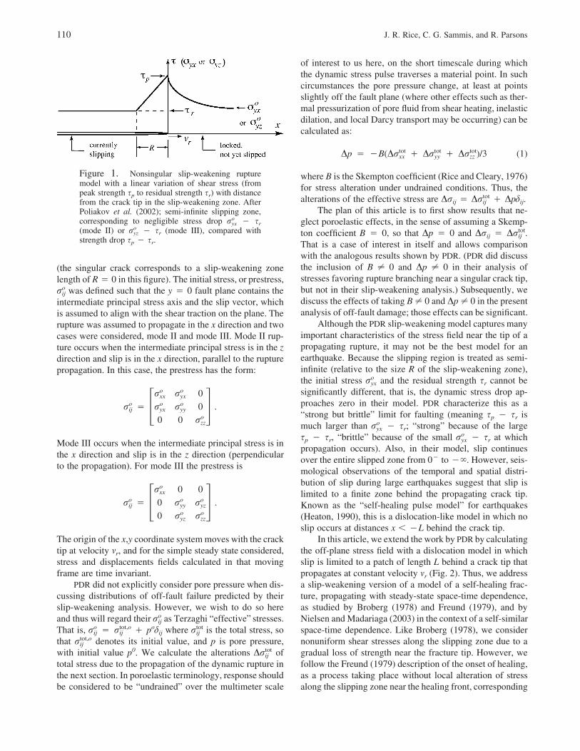
Figure 1. Nonsingular slip-weakening rupturemodel with a linear variation of shear stress (frompeak strength sp to residual strength sr) with distancefrom the crack tip in the slip-weakening zone. AfterPoliakov et al. (2002); semi-infinite slipping zone,corresponding to negligible stress drop � sr
oryx
(mode II) or � sr (mode III), compared withoryz
strength drop sp � sr.
(the singular crack corresponds to a slip-weakening zonelength of R � 0 in this figure). The initial stress, or prestress,
was defined such that the y � 0 fault plane contains theorij
intermediate principal stress axis and the slip vector, whichis assumed to align with the shear traction on the plane. Therupture was assumed to propagate in the x direction and twocases were considered, mode II and mode III. Mode II rup-ture occurs when the intermediate principal stress is in the zdirection and slip is in the x direction, parallel to the rupturepropagation. In this case, the prestress has the form:
o or r 0xx yxo o or � r r 0 .ij yx yy� �o0 0 rzz
Mode III occurs when the intermediate principal stress is inthe x direction and slip is in the z direction (perpendicularto the propagation). For mode III the prestress is
or 0 0xxo o or � 0 r r .ij yy yz� �o o0 r ryz zz
The origin of the x,y coordinate system moves with the cracktip at velocity mr, and for the simple steady state considered,stress and displacements fields calculated in that movingframe are time invariant.
PDR did not explicitly consider pore pressure when dis-cussing distributions of off-fault failure predicted by theirslip-weakening analysis. However, we wish to do so hereand thus will regard their as Terzaghi “effective” stresses.orij
That is, � podij where is the total stress, soo tot,o totr � r rij ij ij
that denotes its initial value, and p is pore pressure,tot,orij
with initial value p0. We calculate the alterations oftotDrij
total stress due to the propagation of the dynamic rupture inthe next section. In poroelastic terminology, response shouldbe considered to be “undrained” over the multimeter scale
of interest to us here, on the short timescale during whichthe dynamic stress pulse traverses a material point. In suchcircumstances the pore pressure change, at least at pointsslightly off the fault plane (where other effects such as ther-mal pressurization of pore fluid from shear heating, inelasticdilation, and local Darcy transport may be occurring) can becalculated as:
tot tot totDp � �B(Dr � Dr � Dr )/3 (1)xx yy zz
where B is the Skempton coefficient (Rice and Cleary, 1976)for stress alteration under undrained conditions. Thus, thealterations of the effective stress are Drij � � Dpdij.
totDrij
The plan of this article is to first show results that ne-glect poroelastic effects, in the sense of assuming a Skemp-ton coefficient B � 0, so that Dp � 0 and Drij � .totDrij
That is a case of interest in itself and allows comparisonwith the analogous results shown by PDR. (PDR did discussthe inclusion of B � 0 and Dp � 0 in their analysis ofstresses favoring rupture branching near a singular crack tip,but not in their slip-weakening analysis.) Subsequently, wediscuss the effects of taking B � 0 and Dp � 0 in the presentanalysis of off-fault damage; those effects can be significant.
Although the PDR slip-weakening model captures manyimportant characteristics of the stress field near the tip of apropagating rupture, it may not be the best model for anearthquake. Because the slipping region is treated as semi-infinite (relative to the size R of the slip-weakening zone),the initial stress and the residual strength sr cannot beoryx
significantly different, that is, the dynamic stress drop ap-proaches zero in their model. PDR characterize this as a“strong but brittle” limit for faulting (meaning sp � sr ismuch larger than � sr; “strong” because of the largeoryx
sp � sr, “brittle” because of the small � sr at whichoryx
propagation occurs). Also, in their model, slip continuesover the entire slipped zone from 0� to ��. However, seis-mological observations of the temporal and spatial distri-bution of slip during large earthquakes suggest that slip islimited to a finite zone behind the propagating crack tip.Known as the “self-healing pulse model” for earthquakes(Heaton, 1990), this is a dislocation-like model in which noslip occurs at distances x � �L behind the crack tip.
In this article, we extend the work by PDR by calculatingthe off-plane stress field with a dislocation model in whichslip is limited to a patch of length L behind a crack tip thatpropagates at constant velocity mr (Fig. 2). Thus, we addressa slip-weakening version of a model of a self-healing frac-ture, propagating with steady-state space-time dependence,as studied by Broberg (1978) and Freund (1979), and byNielsen and Madariaga (2003) in the context of a self-similarspace-time dependence. Like Broberg (1978), we considernonuniform shear stresses along the slipping zone due to agradual loss of strength near the fracture tip. However, wefollow the Freund (1979) description of the onset of healing,as a process taking place without local alteration of stressalong the slipping zone near the healing front, corresponding
Off-Fault Secondary Failure Induced by a Dynamic Slip Pulse 111
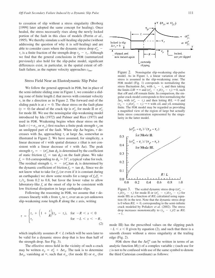
Figure 2. Nonsingular slip-weakening slip-pulsemodel. As in Figure 1, a linear variation of shearstress is assumed in the slip-weakening zone. ThePDR model (Fig. 1) coresponds to normalizing thestress fluctuation Drij with sp � sr and then takingthe limits L/R r � and ( � sr)/(sp � sr) r 0, suchoryx
that x/R and y/R remain finite. In comparison, the sin-gular crack model corresponds to first normalizing theDrij with ( � sr) and then letting R/L r 0 andoryx
(sp � sr)/( � sr) r � with x/L and y/L remainingoryx
finite. The PDR model may be regarded as providinga magnified view of the region of large but actuallyfinite stress concentration represented by the singu-larity in the latter model.
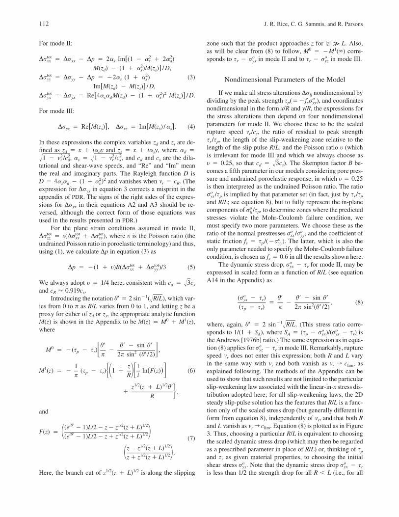
Figure 3. The scaled dynamic stress drop (( �oryx
sr)/(sp � sr) for mode II or ( � sr)/(sp � sr) fororyz
mode III) as a function of R/L calculated using equa-tion (8) in the text. Note that the dynamic stress dropis 0 when R/L � 0, corresponding to the semi-infinitecrack modeled by Poliakov et al. (2002). The stressdrop increases monotonically to (sp � sr)/2 as R/Lr 1.
to cessation of slip without a stress singularity (Broberg[1999] later adopted the same concept for healing). Oncehealed, the stress necessarily rises along the newly lockedportion of the fault in this class of models (Perrin et al.,1995). We thereby simulate a self-healing slip pulse (withoutaddressing the question of why it is self-healing) and areable to consider cases where the dynamic stress drop �oryx
sr is a finite fraction of the strength drop sp � sr . Althoughwe find that the general conclusions in PDR (summarizedpreviously) also hold for the slip-pulse model, significantdifferences exist, in particular, in the spatial extent of off-fault failure, as the rupture velocity approaches clim.
Stress Field Near an Elastodynamic Slip Pulse
We follow the general approach in PDR, but in place ofthe semi-infinite sliding zone in Figure 1, we consider a slid-ing zone of finite length L that moves with constant velocitymr in the x direction as in Figure 2. The forward end of thesliding patch is at x � 0. The shear stress on the fault plane(y � 0) far ahead of the crack tip is for mode II oro or ryx yz
for mode III. We use the nonsingular slip-weakening modelintroduced by Ida (1972) and Palmer and Rice (1973) andused in PDR. Weakening begins when shear stress on thefault s (�ryx or ryz) first reaches a finite peak strength sp onan unslipped part of the fault. When slip Du begins, s de-creases with Du, approaching sr at large Du, somewhat asillustrated in Figure 2. We have assumed, for simplicity, alinear decrease of s with spatial distance x (that is not con-sistent with a linear decrease of s with Du). The peakstrength sp � � ( )tan �p is determined by the coefficientoryy
of static friction (fs � tan �p) on the fault plane. We takefs � 0.6 corresponding to �p � 31�, a typical value for rock.The residual strength sr � � ( )tan �r is determined byoryy
the dynamic coefficient of friction fd � tan �r. Since we donot know what to take for fd (or even if it is constant duringan earthquake) we show some results for a range of fd/fs �sr/sp from 0.2 to 0.8, but favor the lower value to allowlaboratory-like fs at the onset of slip to be consistent withlow frictional dissipation in large earthquake slips.
Following the reasoning in PDR, we assume that s de-creases linearly with x from sp to sr over an as-yet-unknownslip-weakening zone length R along the x axis, writing
xs � 1 � (s � s ), for �R � x � 0r p r� �Rs � �s for �L � x � �R ,r
(2)
which implicitly assumes R � L (which will be seen later tobe valid for a dynamic stress drop that is less than half ofthe strength drop. See Fig. 3).
The effective stress field in the vicinity of such a crackmay be written rij � � Drij. The task is to determineorij
Drij, vanishing at �, such that ryx (for mode II) or ryz (for
mode III) has the prescribed values on the slipping patch�L � x � 0 given by equation (2), and such that there is asmooth closure without a stress singularity at the trailingedge (Fig. 2).
PDR show that the can be written in terms of antotDrij
analytic function M(z) of a complex variable z (such use forz is not to be confused with use of the same symbol to denotethe third Cartesian coordinate) as follows:
112 J. R. Rice, C. G. Sammis, and R. Parsons
For mode II:
tot 2 2Dr � Dr � Dp � 2� Im[(1 � � � 2� )xx xx s s d2M(z ) � (1 � � )M(z )] /D,d s s
tot 2Dr � Dr � Dp � �2� (1 � � ) (3)yy yy s s
Im[M(z ) � M(z )] /D,d stot 2 2Dr � Dr � Re[4� � M(z ) � (1 � � ) M(z )] /D.yx yx s d d s s
For mode III:
Dr � Re[M(z )], Dr � Im[M(z ) /� ]. (4)yz s xz s s
In these expressions the complex variables zd and zs are de-fined as zd � x � i�dy and zs � x � i�sy, where �d �
, �s � , and cd and cs are the dila-2 2 2 21 � v /c 1 � v /c� �r d r s
tational and shear-wave speeds, and “Re” and “Im” meanthe real and imaginary parts. The Rayleigh function D isD � 4�s�d � (1 � )2 and vanishes when mr � cR. (The2�s
expression for Dryx in equation 3 corrects a misprint in theappendix of PDR. The signs of the right sides of the expres-sions for Dryx in their equations A2 and A3 should be re-versed, although the correct form of those equations wasused in the results presented in PDR.)
For the plane strain conditions assumed in mode II,� t( � ), where t is the Poisson ratio (thetot tot totDr Dr Drzz xx yy
undrained Poisson ratio in poroelastic terminology) and thus,using (1), we calculate Dp in equation (3) as
tot totDp � �(1 � t)B(Dr � Dr )/3 (5)xx yy
We always adopt t � 1/4 here, consistent with cd � 3c� s
and cR � 0.919cs.Introducing the notation h� � 2 sin�1( ), which var-R/L�
ies from 0 to p as R/L varies from 0 to 1, and letting z be aproxy for either of zd or zs, the appropriate analytic functionM(z) is shown in the Appendix to be M(z) � M0 � M1(z),where
h� h� � sin h�0M � �(s � s ) � ,p r � 2 �p 2p sin (h�/2)
1 z 11M (z) � � (s � s ) 1 � ln(F(z)) (6)p r �� �� �p R i
1/2 1/2z (z � L) h�� ,�R
and
ih� 1/2 1/2(e �1)L/2� z� z (z�L)F(z) � � ih� 1/2 1/2�(e �1)L/2� z� z (z�L) (7)
1/2 1/2z� z (z�L).� 1/2 1/2�z� z (z�L)
Here, the branch cut of z1/2(z � L)1/2 is along the slipping
zone such that the product approaches z for |z| k L. Also,as will be clear from (8) to follow, M0 � �M1(�) corre-sponds to sr � in mode II and to sr � in mode III.o or ryx yz
Nondimensional Parameters of the Model
If we make all stress alterations Drij nondimensional bydividing by the peak strength sp(��fs ), and coordinatesoryy
nondimensional in the form x/R and y/R, the expressions forthe stress alterations then depend on four nondimensionalparameters for mode II. We choose these to be the scaledrupture speed mr/cs, the ratio of residual to peak strengthsr/sp, the length of the slip-weakening zone relative to thelength of the slip pulse R/L, and the Poisson ratio t (whichis irrelevant for mode III and which we always choose ast � 0.25, so that cd � ). The Skempton factor B be-3c� s
comes a fifth parameter in our models considering pore pres-sure and undrained poroelastic response, in which t � 0.25is then interpreted as the undrained Poisson ratio. The ratio
/sp is implied by that parameter set (in fact, just by sr/sporyx
and R/L; see equation 8), but to fully represent the in-planecomponents of /sp, to determine zones where the predictedorij
stresses violate the Mohr-Coulomb failure condition, wemust specify two more parameters. We choose these as theratio of the normal prestresses , and the coefficient ofo or /rxx yy
static friction fs � sp/(� ). The latter, which is also theoryy
only parameter needed to specify the Mohr-Coulomb failurecondition, is chosen as fs � 0.6 in all the results shown here.
The dynamic stress drop, � sr for mode II, may beoryx
expressed in scaled form as a function of R/L (see equationA14 in the Appendix) as
o(r � s ) h� h� � sin h�yx r� � , (8)2(s � s ) p 2p sin (h�/2)p r
where, again, h� � 2 sin�1 . (This stress ratio corre-R/L�sponds to 1/(1 � SA), where SA � (sp � )/( � sr) iso or ryx yx
the Andrews [1976b] ratio.) The same expression as in equa-tion (8) applies for � sr in mode III. Remarkably, ruptureoryz
speed mr does not enter this expression; both R and L varyin the same way with mr and both vanish as mr r clim, asexplained following. The methods of the Appendix can beused to show that such results are not limited to the particularslip-weakening law associated with the linear-in-x stress dis-tribution adopted here; for all slip-weakening laws, the 2Dsteady slip-pulse solution has the features that R/L is a func-tion only of the scaled stress drop (but generally different inform from equation 8), independently of mr, and that both Rand L vanish as mr r clim. Equation (8) is plotted as in Figure3. Thus, choosing a particular R/L is equivalent to choosingthe scaled dynamic stress drop (which may then be regardedas a prescribed parameter in place of R/L) or, thinking of sp
and sr as given material properties, to choosing the initialshear stress . Note that the dynamic stress drop � sr
o or ryx yx
is less than 1/2 the strength drop for all R � L (i.e., for all
Off-Fault Secondary Failure Induced by a Dynamic Slip Pulse 113
h� � p), and that ( � sr)/(sp � sr) r 0 as R/L r 0oryx
(h� r 0), corresponding to the semi-infinite crack modeledby PDR.
The size of the slip-weakening zone, R, depends on thefracture energy G, the shear modulus l, the strength drop(sp � sr), the scaled rupture velocity mr/cs, and the dynamicstress drop (which we parameterize using h� � 2 sin�1
as previously). In this slip-weakening context, G isR/L�defined by G � �[s(Du) � sr]d(Du) (Palmer and Rice,1973; Rice, 1980), where s(Du) is the slip-weakening func-tion implied through the elasticity solution for our assumedlinear-in-x stress distribution in Figure 2 and the integralextends to sufficiently large slips Du that s(Du) becomescoincident with sr. We show in the Appendix, in equations(A25) and (A26), that
lG F(v )rR � , (9)2(s � s ) h(h�)p r
where
h� h� � sin h� h� � sin h� cos h�h(h�) � � , (10)� 2 � � 4 �p 2p sin (h�/2) 4 sin (h�/2)
which varies only modestly, from h(0�) � 16/9p � 0.566to h(p) � p/8 � 0.393, and
2D / [� (1 � � )] for mode IIs sF(v ) � (11)r �� for mode III.s
Here, D � 4�s�d � (1 � )2 is the Rayleigh factor defined2�s
previously. The functions F(mr) diminish with rupture speedand vanish when mr r clim, with the following limits:
1/(1 � t) when v � 0r for mode II�0 when v � cr RF(v ) �r 1 when v � 0r� for mode III,�0 when v � cr s
where t is the Poisson ratio. The ratio F(mr)/F(0) correspondsto what is called 1/fII(mr) for mode II, and 1/fIII(mr) for modeIII, in Rice (1980) and PDR.
We write the value of R at low speed (mr � 0�), but atthe same fixed R/L (or fixed stress drop), as Ro where Ro �
. Hence,2[lG/(s � s ) ]F(0)/h(h�)p r
R F(v ) (1 � t)Dr� � (12)2R F(0) � (1 � � )o s s
for mode II, and R/Ro � �s for mode III. Thus R/Ro is afunction of mr only. A slipping length Lo may be similarlydefined, just by equating Ro/Lo to the fixed R/L. Then itfollows that L/Lo � R/R0, so that L/Lo is the same functionof mr as in equation (12).
Because Ro depends on R/L, we choose to normalize all
lengths in the problem by the value of Ro when L/R r �(that is, when the dynamic stress drop is a negligible fractionof the strength drop), which we call . This is obviouslyR*oinvariant to mr and to the magnitude of the stress drop. Be-cause h(h�) � h(0�) � 16/9p, we havelim
L/Rr�
9pF(0) lG 9p lGR* � � , (13)o 2 216 (s � s ) 16(1 � t) (s � s )p r p r
for mode II, exactly as in PDR, and the (1 � t) is deletedfor mode III. Hence, using equations (9) and (13), we scaleR for mode II as
R 16(1 � t) F(v )r� (14)
R* 9p h(h�)o
and L as L/ � (L/R)(R/ ), where L/R is one of the givenR* R*o o
parameters. For mode III, the (1 � t) is again deleted. (Notethat our coincides with what PDR called Ro, because theyR*odealt only with the h� � 0 case of vanishing scaled stressdrop.)
As in PDR, R decreases to zero as mr increases to itslimiting value clim. Because L/R is fixed for a given, scaled,stress drop by equation (8), L also approaches zero. How-ever, the final slip displacement d that is locked-in on healingis independent of mr, so that our slip-pulse solution ap-proaches that of a step Volterra dislocation moving at speedclim. That is because, as we show in equation (A23),
2G 16(1 � t) (s � s )p rd � � R* , (15)oo or � s 9p (r � s )lyx r yx r
for mode II, where the latter form uses (13) also. Thus, thelocked-in displacement depends only on the fracture energyand dynamic stress drop but is independent of the velocity.This result (15) also holds for mode III, which differs onlyby the change of stress drop to � sr and deletion of theoryz
(1 � t) in the latter form. The result, rewritten as �or dyx
srd � G, is easy to interpret. It says that the work ofor dyx
the remote stress field in advance of the rupture front overa unit area is balanced by the total dissipation, which is thesum of srd in friction dissipation at the residual level, plusG by stresses s(Du) � sr in excess of residual.
As suggested, there is a certain slip-weakening relations � s(Du) implied by our analysis, which we have simplifiedby assuming a linear variation of stress with distance as inFigure 2, corresponding to a specified fracture energy G,which is interpretable as G � �[s(Du) � sr]d(Du). The re-sulting weakening function s(Du) was plotted by Palmer andRice (1973) for the R/L � 0 limit and mr � 0� case thatthey considered. Rice (1980) showed, again for the R/L �0 limit, that for dynamic propagation, the function s(Du)implied by this procedure is independent of mr. A similarresult holds here: For a given scaled dynamic stress drop,
114 J. R. Rice, C. G. Sammis, and R. Parsons
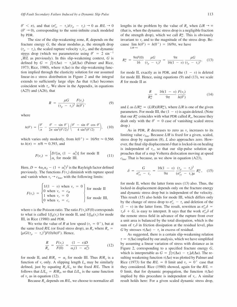
Figure 4. Mohr circle in terms of effective stress,illustrating the condition for Coulomb failure on themost favorably oriented plane.
hence given R/L and given fracture energy G, the impliedslip-weakening function is independent of mr . However, inour present work, the precise form of that implied s(Du)depends on R/L (although it starts at the same sp, finishes atthe same sr and has the same integral G for all R/L). Weshow in the Appendix how to determine s(Du) and, by com-paring results for the limit cases R/L � 0 and R/L � 1 (seethe final figure of the Appendix), we demonstrate that thedependence on R/L is very weak, suggesting therefore thatit may be safely neglected.
Off-Plane Coulomb Failure Induced by aSlip Pulse: Mode II
The potential for bending or forking of the slip-pulseonto planes intersecting a singular crack tip is exactly ascalculated by PDR for the semi-infinite crack, because thestress field in the immediate vicinity of the tip is the samein both cases. However, the spatial extent of Coulomb failureon slip surfaces removed from the crack tip can be quitedifferent for the two cases. Slip will occur when the Cou-lomb stress on a plane, defined as s � fsrn, is greater than0. (Recall that rn is negative for compression and, consid-ering pore pressure, the stresses are effective stresses.) Wewill produce figures similar to figures 11 and 13 in PDR toeffect a direct comparison between the mode II finite slippulse modeled here and the mode II semi-infinite crack mod-eled by PDR. Those figures in PDR explore the effects ofparameters , mr/cs, and sr/sp on the spatial distributiono or /rxx yy
of Coulomb failure. We use the same range of parametersas in figures 11 and 13 in PDR for a range of the new pa-rameter R/L � 0.001, 0.1, 0.5, and 0.9. The figures in PDRcorrespond to the case R/L � 0. We explore mode III in thenext section.
The new figures were calculated as follows: All stresseswere scaled by sp. The diagonal elements of the remote stressfield are then /sp � �1/fs, where we take fs � 0.6 fororyy
the static coefficient of friction, and /sp � ( ) /o o o or r /r rxx xx yy yy
sp, where the stress ratio is a given parameter. The remoteshear stress is given by (A14) in the Appendix which, scaledby sp, gives
or h� h� � sin h� s syx r r� � 1 � � , (16)� 2 � � �s p 2p sin (h�/2) s sp p p
where sr/sp and h� � 2 sin�1 are given parameters.R/L�The changes in effective stress due to the cut, Drij, were
calculated using equations (3), (5), (6), and (7), with B � 0in (5) so that Dp � 0 and Drij � (Figs. 5 to 10), andtotDrij
subsequently with B � 0 (Figs. 11 and 12). Note that thestresses in these equations have the factor (sp � sr) which,because we are scaling all stresses by sp, becomes (1�sr/sp).The lengths z, R, and L in these equations were scaled by
as discussed previously. The stress components were cal-R*oculated as rij � �Drij on a grid of points �2 � x/or R*ij o
� 2, �2 � y/ � 2. At each grid point, we asked whetherR*ofrictional sliding had occurred on the most favorably ori-ented plane. This is most easily visualized using the Mohrcircle diagram in Figure 4 for which the principal stressesare r1 � S � smax and r2 � S � smax, where S � (1/2)(rxx
� ryy) and smax � (1/2)[(rxx � ryy)2 � 1/2. The angle24r ]yx
w between the r1 and the x axis is w � (1/2) tan�1 [2ryx/(rxx � ryy)].
Referring to the Mohr circle in terms of effective stressin Figure 4, slip first occurs when the circle touches thefriction line s � �rn tan �p. This occurs when smax � �Ssin �p. Hence, for any stress state where smax � �S sin �p,slip will have occurred on the most favorable plane, andpossibly others. We defined sCoulomb � �S sin �p and, ateach grid point, computed the ratio smax/sCoulomb. Slip willhave occurred at any point where smax/sCoulomb � 1. Thecritical planes on which slip first occurs make angle of�(1/2)(p/2 � �p) with respect to r1. For �p � 31�, thecritical planes are oriented at angles w � 29.5� relative tothe x axis. These planes are indicated as line segments onthe contour plots of smax/sCoulomb. We also check to see ifthe least principal stress may have turned positive, that is,tensile.
Effect of Rupture Velocity, Slip-Weakening ZoneSize, and the Orientation of the Initial Stress Field
The effects of rupture velocity mr/cs, the slip-weakeningzone size R/L, and the initial stress ratio on the off-o or /rxx yy
plane stress field are explored in Figures 5 through 9 for thecase B � 0. These figures are formatted as in PDR wherethe ratio smax/sCoulomb is contoured, and areas where this ratiois greater than 1 are lightly shaded. Within this lightly
Off-Fault Secondary Failure Induced by a Dynamic Slip Pulse 115
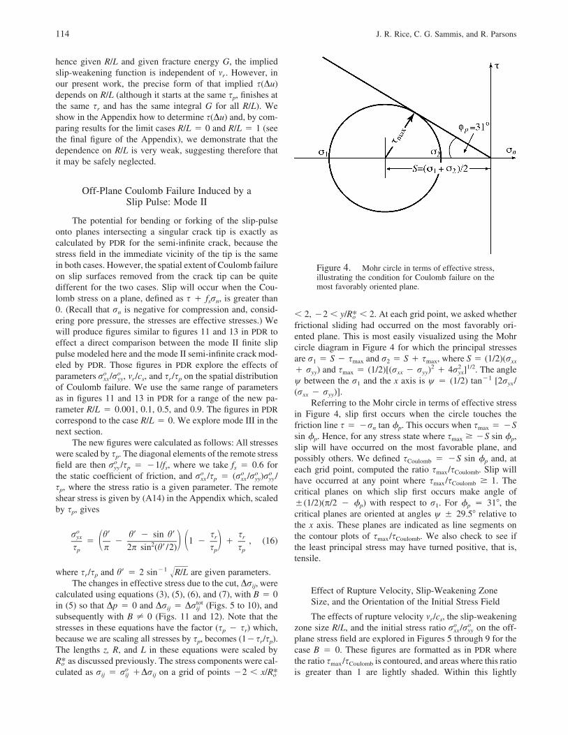
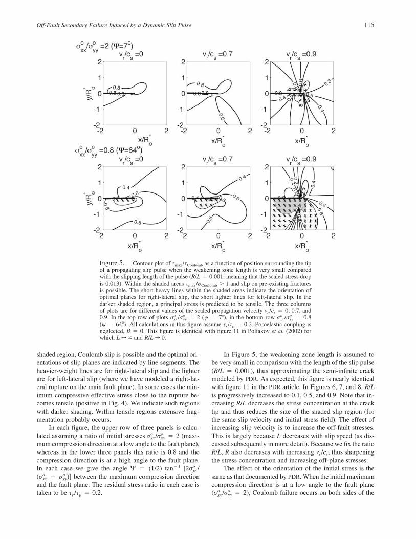
Figure 5. Contour plot of smax/sCoulomb as a function of position surrounding the tipof a propagating slip pulse when the weakening zone length is very small comparedwith the slipping length of the pulse (R/L � 0.001, meaning that the scaled stress dropis 0.013). Within the shaded areas smax/rCoulomb � 1 and slip on pre-existing fracturesis possible. The short heavy lines within the shaded areas indicate the orientation ofoptimal planes for right-lateral slip, the short lighter lines for left-lateral slip. In thedarker shaded region, a principal stress is predicted to be tensile. The three columnsof plots are for different values of the scaled propagation velocity mr/cs � 0, 0.7, and0.9. In the top row of plots � 2 (w � 7�), in the bottom row � 0.8o o o or /r r /rxx yy xx yy
(w � 64�). All calculations in this figure assume sr/sp � 0.2. Poroelastic coupling isneglected, B � 0. This figure is identical with figure 11 in Poliakov et al. (2002) forwhich L r � and R/L r 0.
shaded region, Coulomb slip is possible and the optimal ori-entations of slip planes are indicated by line segments. Theheavier-weight lines are for right-lateral slip and the lighterare for left-lateral slip (where we have modeled a right-lat-eral rupture on the main fault plane). In some cases the min-imum compressive effective stress close to the rupture be-comes tensile (positive in Fig. 4). We indicate such regionswith darker shading. Within tensile regions extensive frag-mentation probably occurs.
In each figure, the upper row of three panels is calcu-lated assuming a ratio of initial stresses � 2 (maxi-o or /rxx yy
mum compression direction at a low angle to the fault plane),whereas in the lower three panels this ratio is 0.8 and thecompression direction is at a high angle to the fault plane.In each case we give the angle W � (1/2) tan�1 [ o2r /yx
] between the maximum compression directiono o(r � r )xx yy
and the fault plane. The residual stress ratio in each case istaken to be sr/sp � 0.2.
In Figure 5, the weakening zone length is assumed tobe very small in comparison with the length of the slip pulse(R/L � 0.001), thus approximating the semi-infinite crackmodeled by PDR. As expected, this figure is nearly identicalwith figure 11 in the PDR article. In Figures 6, 7, and 8, R/Lis progressively increased to 0.1, 0.5, and 0.9. Note that in-creasing R/L decreases the stress concentration at the cracktip and thus reduces the size of the shaded slip region (forthe same slip velocity and initial stress field). The effect ofincreasing slip velocity is to increase the off-fault stresses.This is largely because L decreases with slip speed (as dis-cussed subsequently in more detail). Because we fix the ratioR/L, R also decreases with increasing mr/cs, thus sharpeningthe stress concentration and increasing off-plane stresses.
The effect of the orientation of the initial stress is thesame as that documented by PDR. When the initial maximumcompression direction is at a low angle to the fault plane( � 2), Coulomb failure occurs on both sides of theo or /rxx yy
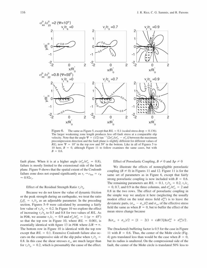
116 J. R. Rice, C. G. Sammis, and R. Parsons
Figure 6. The same as Figure 5, except that R/L � 0.1 (scaled stress drop � 0.136).The larger weakening zone length produces less off-fault stress at a comparable slipvelocity. Note that the angle W � (1/2) tan�1 [ /( � )] between the maximumo o o2r r ryx xx yy
precompression direction and the fault plane is slightly different for different values ofR/L; now W � 10� in the top row and 59� in the bottom. Like in all of Figures 5 to10 here, B � 0, although Figure 11 to follow examines the same cases, but withB � 0.6.
fault plane. When it is at a higher angle ( � 0.8),o or /rxx yy
failure is mostly limited to the extensional side of the faultplane. Figure 9 shows that the spatial extent of the Coulombfailure zone does not expand significantly as mr r clim � cR
� 0.92cs.
Effect of the Residual Strength Ratio sr/sp
Because we do not know the value of dynamic frictionor the peak strength during an earthquake, we treat the ratiofd/fs � sr/sp as an adjustable parameter. In the precedingsection, Figures 5–9 were calculated by assuming a fairlylow value of sr/sp � 0.2. In Figure 10 we explore the effectof increasing sr/sp to 0.5 and 0.8 for two values of R/L. Asin PDR, we assume mr/cs � 0.9 and � 1 (w � 45�)o or /rxx yy
so that the top row in Figure 10, where R/L � 0.001, isessentially identical with figure 13 in PDR where L/R r �.The bottom row in Figure 10 is identical with the top rowexcept that R/L � 0.1. Extensive Coulomb failure also oc-curs on the compressive side of the slip pulse when sr/sp �0.8. In this case the shear stresses ryx are much larger thanfor sr/sp � 0.2, which is presumably the cause of the effect.
Effect of Poroelastic Coupling, B � 0 and Dp � 0
We illustrate the effects of nonnegligible poroelasticcoupling (B � 0) in Figures 11 and 12. Figure 11 is for thesame set of parameters as in Figure 6, except that fairlystrong poroelastic coupling is now included with B � 0.6.The remaining parameters are R/L � 0.1, sr/sp � 0.2, mr/cs
� 0, 0.7, and 0.9 in the three columns, and � 2 ando or /rxx yy
0.8 in the two rows. The effect of poroelastic coupling inthe simple way we analyze it here (neglecting the usuallymodest effect on the total stress field ) is to leave thetotrij
deviatoric parts, (rxx � ryy)/2 and ryx, of the effective stressfield the same as when B � 0, but to buffer the effect of themean stress change because
tot totD(r � r )/2 � [1 � 2(1 � t)B/3]D(r � r )/2 .xx yy xx yy
The (bracketed) buffering factor is 0.5 for the case in Figure11 with B � 0.6. Thus, the center of the Mohr circle (Fig.4) gets translated less than would be the case when B � 0,but its radius is unaltered. On the compressional side of thefault, the center of the Mohr circle is translated 50% less to
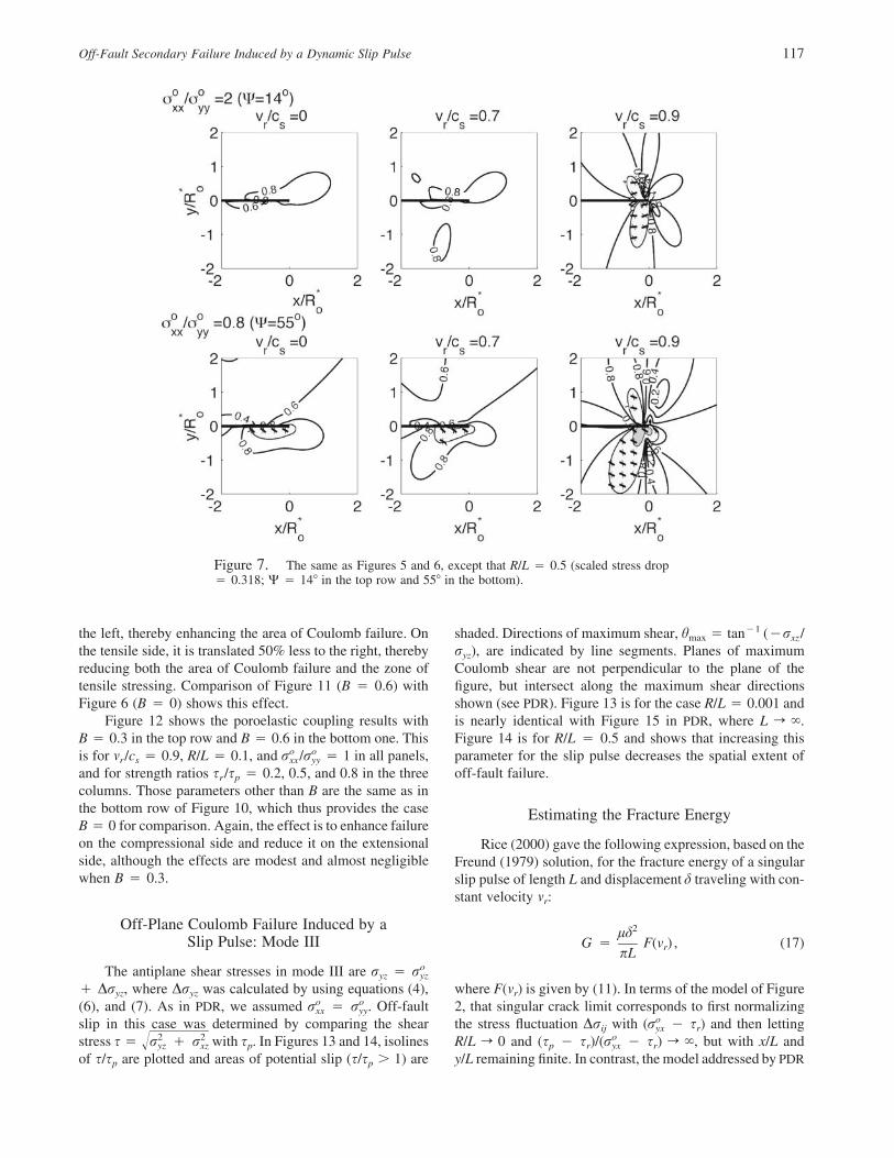
Off-Fault Secondary Failure Induced by a Dynamic Slip Pulse 117
Figure 7. The same as Figures 5 and 6, except that R/L � 0.5 (scaled stress drop� 0.318; W � 14� in the top row and 55� in the bottom).
the left, thereby enhancing the area of Coulomb failure. Onthe tensile side, it is translated 50% less to the right, therebyreducing both the area of Coulomb failure and the zone oftensile stressing. Comparison of Figure 11 (B � 0.6) withFigure 6 (B � 0) shows this effect.
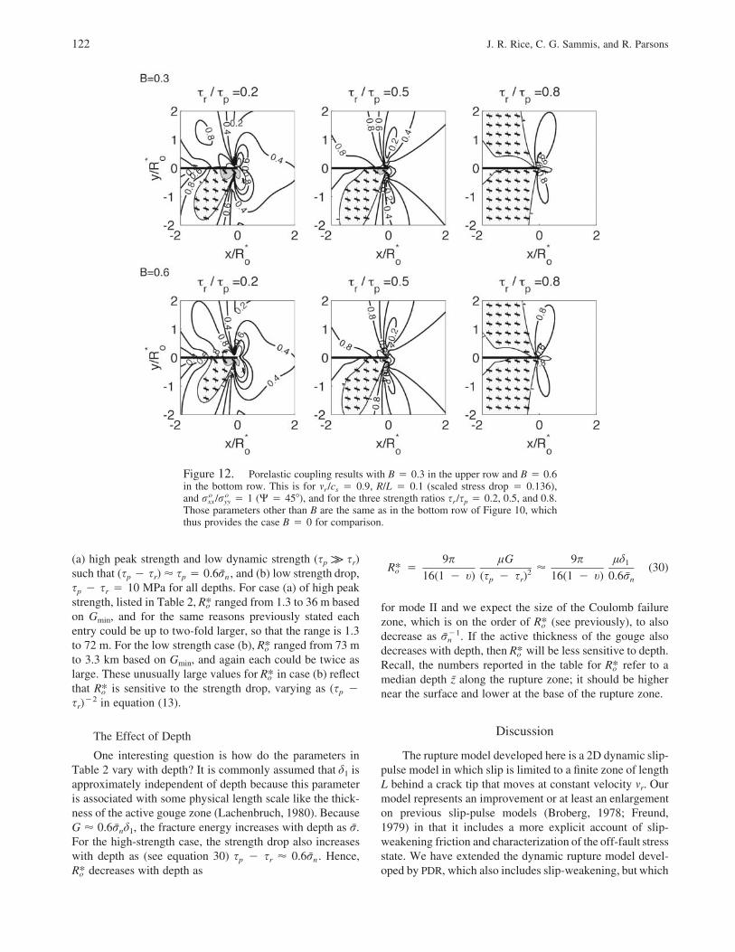
Figure 12 shows the poroelastic coupling results withB � 0.3 in the top row and B � 0.6 in the bottom one. Thisis for mr/cs � 0.9, R/L � 0.1, and � 1 in all panels,o or /rxx yy
and for strength ratios sr/sp � 0.2, 0.5, and 0.8 in the threecolumns. Those parameters other than B are the same as inthe bottom row of Figure 10, which thus provides the caseB � 0 for comparison. Again, the effect is to enhance failureon the compressional side and reduce it on the extensionalside, although the effects are modest and almost negligiblewhen B � 0.3.
Off-Plane Coulomb Failure Induced by aSlip Pulse: Mode III
The antiplane shear stresses in mode III are ryz � oryz
� Dryz, where Dryz was calculated by using equations (4),(6), and (7). As in PDR, we assumed . Off-faulto or � rxx yy
slip in this case was determined by comparing the shearstress s � with sp. In Figures 13 and 14, isolines2 2r � r� yz xz
of s/sp are plotted and areas of potential slip (s/sp � 1) are
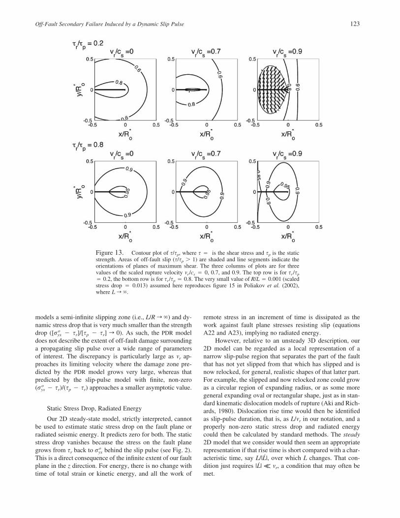
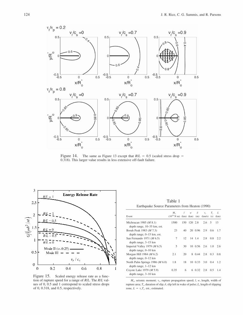
shaded. Directions of maximum shear, hmax � tan�1 (�rxz/ryz), are indicated by line segments. Planes of maximumCoulomb shear are not perpendicular to the plane of thefigure, but intersect along the maximum shear directionsshown (see PDR). Figure 13 is for the case R/L � 0.001 andis nearly identical with Figure 15 in PDR, where L r �.Figure 14 is for R/L � 0.5 and shows that increasing thisparameter for the slip pulse decreases the spatial extent ofoff-fault failure.
Estimating the Fracture Energy
Rice (2000) gave the following expression, based on theFreund (1979) solution, for the fracture energy of a singularslip pulse of length L and displacement d traveling with con-stant velocity mr:
2ldG � F(v ) , (17)r
pL
where F(mr) is given by (11). In terms of the model of Figure2, that singular crack limit corresponds to first normalizingthe stress fluctuation Drij with ( � sr) and then lettingoryx
R/L r 0 and (sp � sr)/( � sr) r �, but with x/L andoryx
y/L remaining finite. In contrast, the model addressed by PDR

118 J. R. Rice, C. G. Sammis, and R. Parsons
Figure 8. The same as Figures 5, 6, and 7, except that R/L � 0.9 (scaled stressdrop � 0.459; W � 17� in the top row and 53� in the bottom row).
(Fig. 1) corresponds to normalizing the stress fluctuationDrij with sp � sr and then taking the same limits as previ-ously, now more naturally expressed as L/R r � and ( oryx
� sr)/(sp � sr) r 0, but now such that x/R and y/R remainfinite in the limit. The PDR model may be regarded as pro-viding a magnified view of the region of large but actuallyfinite stress concentration that is represented by the un-bounded term of the singular crack model. Rice (2000) usedHeaton’s (1990) estimates of L, d, and mr for seven earth-quakes to calculate from (17) an average value of G � 2MJ/m2.
We now repeat this analysis using our more generalresults for the slip-weakening slip pulse. We begin withequation (A24),
2h(h�) (s � s ) Rp rG � , (18)F(v ) lr
where h(h�) is given by equation (10) and F(mr) by (11).Equation (A21) can be used to write:
4ld 4 sin (h�/2)s � s � F(v ) . (19)p r rR h� � sin h� cos h�
Also, we use R � L sin2(h�/2) to change the length scale toL, and use (10) for h(mr/cs,h�), to get:
2G 4p sin (h�/2)G* � �2 � �(ld /pL) h� � sin h� cos h� (20)
h� h� � sin h�� F(v )r� 2 �p 2p sin (h�/2)
The product of the h�-dependent factors in (20) varies from1 when h� r 0 (i.e., when R/L r 0), thus verifying (17) inthat limit, to 2 when h� � p (R/L � 1). Equation (20) isplotted in Figure 15. For R/L � 0, G* decreases smoothlyfrom 1/(1 � t) (mode II) or 1 (mode III), when mr � 0�
toward 0 when mr � clim. The effect of increasing R/L is toincrease G*. The maximum increase is a factor of 2 (for bothmodes II and III) when R � L.
Whereas the scaled fracture energy G* decreasessmoothly to 0 with increasing rupture speed, this is becauseit is scaled by L, which itself decreases to 0. The unscaledfracture energy G is independent of the rupture speed for agiven, speed-independent, slip-weakening function s(Du).
Interpretation of Seismically ObservedSlip Pulses
Following Rice (2000), we used the estimates of L, d,and mr given by Heaton (1990) from seismic slip inversionsfor seven events (Table 1) to calculate G, � sr, slip-orxy
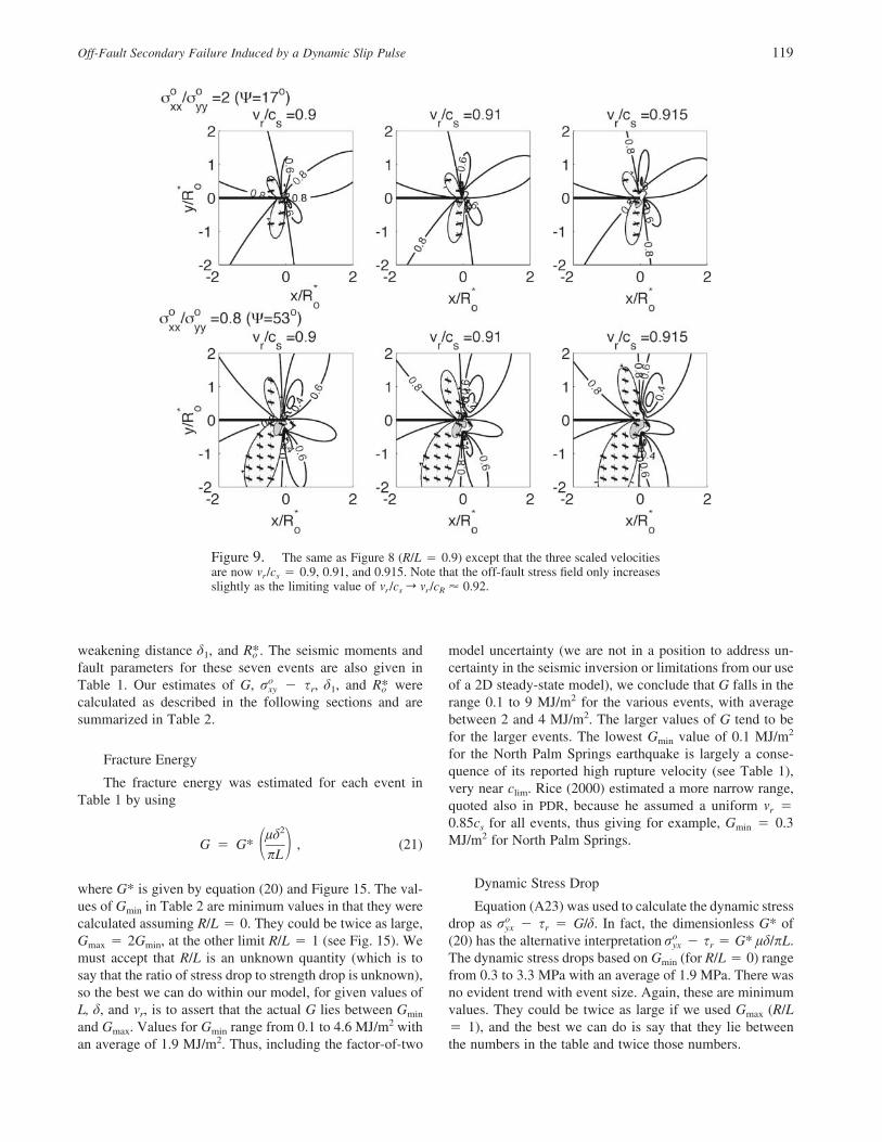
Off-Fault Secondary Failure Induced by a Dynamic Slip Pulse 119
Figure 9. The same as Figure 8 (R/L � 0.9) except that the three scaled velocitiesare now mr/cs � 0.9, 0.91, and 0.915. Note that the off-fault stress field only increasesslightly as the limiting value of mr/cs r mr/cR � 0.92.
weakening distance d1, and . The seismic moments andR*ofault parameters for these seven events are also given inTable 1. Our estimates of G, � sr, d1, and wereor R*xy o
calculated as described in the following sections and aresummarized in Table 2.
Fracture Energy
The fracture energy was estimated for each event inTable 1 by using
2ldG � G* , (21)� �pL
where G* is given by equation (20) and Figure 15. The val-ues of Gmin in Table 2 are minimum values in that they werecalculated assuming R/L � 0. They could be twice as large,Gmax � 2Gmin, at the other limit R/L � 1 (see Fig. 15). Wemust accept that R/L is an unknown quantity (which is tosay that the ratio of stress drop to strength drop is unknown),so the best we can do within our model, for given values ofL, d, and mr, is to assert that the actual G lies between Gmin
and Gmax. Values for Gmin range from 0.1 to 4.6 MJ/m2 withan average of 1.9 MJ/m2. Thus, including the factor-of-two
model uncertainty (we are not in a position to address un-certainty in the seismic inversion or limitations from our useof a 2D steady-state model), we conclude that G falls in therange 0.1 to 9 MJ/m2 for the various events, with averagebetween 2 and 4 MJ/m2. The larger values of G tend to befor the larger events. The lowest Gmin value of 0.1 MJ/m2
for the North Palm Springs earthquake is largely a conse-quence of its reported high rupture velocity (see Table 1),very near clim. Rice (2000) estimated a more narrow range,quoted also in PDR, because he assumed a uniform mr �0.85cs for all events, thus giving for example, Gmin � 0.3MJ/m2 for North Palm Springs.
Dynamic Stress Drop
Equation (A23) was used to calculate the dynamic stressdrop as � sr � G/d. In fact, the dimensionless G* oforyx
(20) has the alternative interpretation � sr � G* ld/pL.oryx
The dynamic stress drops based on Gmin (for R/L � 0) rangefrom 0.3 to 3.3 MPa with an average of 1.9 MPa. There wasno evident trend with event size. Again, these are minimumvalues. They could be twice as large if we used Gmax (R/L� 1), and the best we can do is say that they lie betweenthe numbers in the table and twice those numbers.
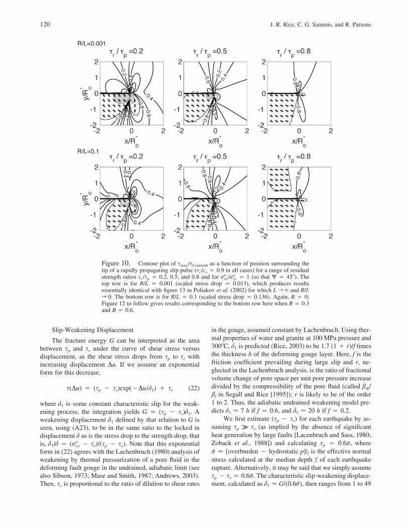
120 J. R. Rice, C. G. Sammis, and R. Parsons
Figure 10. Contour plot of smax/sCoulomb as a function of position surrounding thetip of a rapidly propagating slip pulse (mr/cs � 0.9 in all cases) for a range of residualstrength ratios sr/sp � 0.2, 0.5, and 0.8 and for � 1 (so that W � 45�). Theo or /rxx yy
top row is for R/L � 0.001 (scaled stress drop � 0.013), which produces resultsessentially identical with figure 13 in Poliakov et al. (2002) for which L r � and R/Lr 0. The bottom row is for R/L � 0.1 (scaled stress drop � 0.136). Again, B � 0;Figure 12 to follow gives results corresponding to the bottom row here when B � 0.3and B � 0.6.
Slip-Weakening Displacement
The fracture energy G can be interpreted as the areabetween sp and sr under the curve of shear stress versusdisplacement, as the shear stress drops from sp to sr withincreasing displacement Du. If we assume an exponentialform for this decrease,
s(Du) � (s � s )exp(�Du/d ) � s (22)p r 1 r
where d1 is some constant characteristic slip for the weak-ening process, the integration yields G � (sp � sr)d1. Aweakening displacement d1 defined by that relation to G isseen, using (A23), to be in the same ratio to the locked indisplacement d as is the stress drop to the strength drop, thatis, d1/d � ( � sr)/(sp � sr). Note that this exponentialoryx
form in (22) agrees with the Lachenbruch (1980) analysis ofweakening by thermal pressurization of a pore fluid in thedeforming fault gouge in the undrained, adiabatic limit (seealso Sibson, 1973; Mase and Smith, 1987; Andrews, 2003).Then, sr is proportional to the ratio of dilation to shear rates
in the gouge, assumed constant by Lachenbruch. Using ther-mal properties of water and granite at 100 MPa pressure and300�C, d1 is predicted (Rice, 2003) to be 1.7 (1 � r)/f timesthe thickness h of the deforming gouge layer. Here, f is thefriction coefficient prevailing during large slip and r, ne-glected in the Lachenbruch analysis, is the ratio of fractionalvolume change of pore space per unit pore pressure increasedivided by the compressibility of the pore fluid (called b�/bf in Segall and Rice [1995]); r is likely to be of the order1 to 2. Thus, the adiabatic undrained weakening model pre-dicts d1 � 7 h if f � 0.6, and d1 � 20 h if f � 0.2.
We first estimate (sp � sr) for each earthquake by as-suming sp k sr (as implied by the absence of significantheat generation by large faults [Lacenbruch and Sass, 1980;Zoback et al., 1988]) and calculating sp � 0.6 , wherer̄
� [overburden � hydrostatic p]|z̄ is the effective normalr̄stress calculated at the median depth z̄ of each earthquakerupture. Alternatively, it may be said that we simply assumesp � sr � 0.6 . The characteristic slip-weakening displace-r̄ment, calculated as d1 � G/(0.6 ), then ranges from 1 to 49r̄
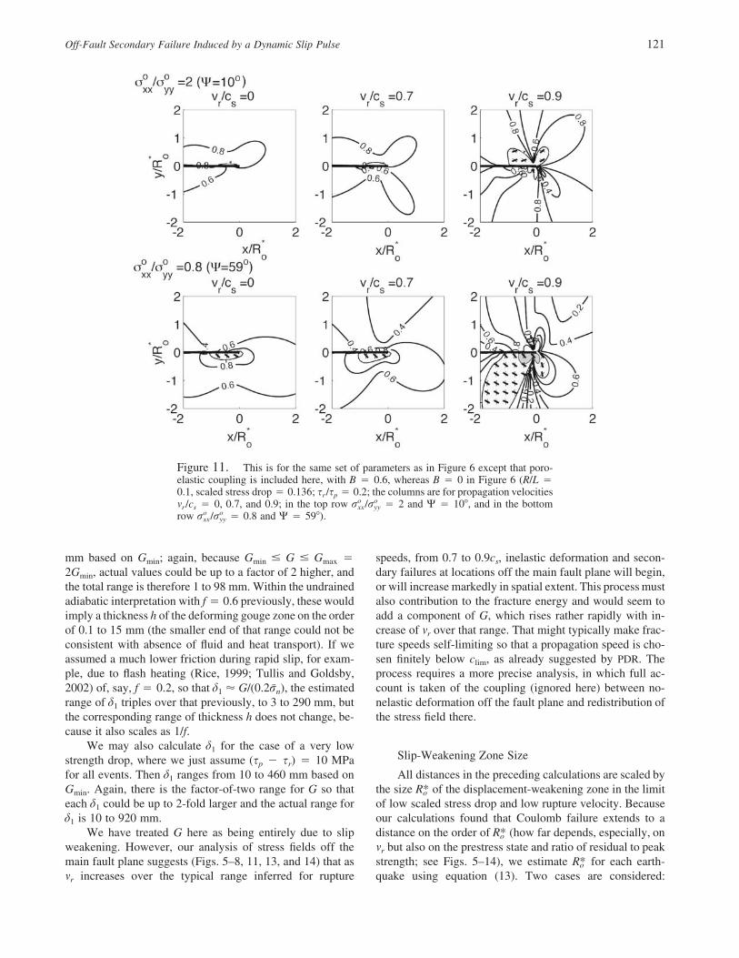
Off-Fault Secondary Failure Induced by a Dynamic Slip Pulse 121
Figure 11. This is for the same set of parameters as in Figure 6 except that poro-elastic coupling is included here, with B � 0.6, whereas B � 0 in Figure 6 (R/L �0.1, scaled stress drop � 0.136; sr/sp � 0.2; the columns are for propagation velocitiesmr/cs � 0, 0.7, and 0.9; in the top row � 2 and W � 10�, and in the bottomo or /rxx yy
row � 0.8 and W � 59�).o or /rxx yy
mm based on Gmin; again, because Gmin � G � Gmax �2Gmin, actual values could be up to a factor of 2 higher, andthe total range is therefore 1 to 98 mm. Within the undrainedadiabatic interpretation with f � 0.6 previously, these wouldimply a thickness h of the deforming gouge zone on the orderof 0.1 to 15 mm (the smaller end of that range could not beconsistent with absence of fluid and heat transport). If weassumed a much lower friction during rapid slip, for exam-ple, due to flash heating (Rice, 1999; Tullis and Goldsby,2002) of, say, f � 0.2, so that d1 � G/(0.2 ), the estimatedr̄n
range of d1 triples over that previously, to 3 to 290 mm, butthe corresponding range of thickness h does not change, be-cause it also scales as 1/f.
We may also calculate d1 for the case of a very lowstrength drop, where we just assume (sp � sr) � 10 MPafor all events. Then d1 ranges from 10 to 460 mm based onGmin. Again, there is the factor-of-two range for G so thateach d1 could be up to 2-fold larger and the actual range ford1 is 10 to 920 mm.
We have treated G here as being entirely due to slipweakening. However, our analysis of stress fields off themain fault plane suggests (Figs. 5–8, 11, 13, and 14) that asmr increases over the typical range inferred for rupture
speeds, from 0.7 to 0.9cs, inelastic deformation and secon-dary failures at locations off the main fault plane will begin,or will increase markedly in spatial extent. This process mustalso contribution to the fracture energy and would seem toadd a component of G, which rises rather rapidly with in-crease of mr over that range. That might typically make frac-ture speeds self-limiting so that a propagation speed is cho-sen finitely below clim, as already suggested by PDR. Theprocess requires a more precise analysis, in which full ac-count is taken of the coupling (ignored here) between no-nelastic deformation off the fault plane and redistribution ofthe stress field there.
Slip-Weakening Zone Size
All distances in the preceding calculations are scaled bythe size of the displacement-weakening zone in the limitR*oof low scaled stress drop and low rupture velocity. Becauseour calculations found that Coulomb failure extends to adistance on the order of (how far depends, especially, onR*omr but also on the prestress state and ratio of residual to peakstrength; see Figs. 5–14), we estimate for each earth-R*oquake using equation (13). Two cases are considered:
122 J. R. Rice, C. G. Sammis, and R. Parsons
Figure 12. Porelastic coupling results with B � 0.3 in the upper row and B � 0.6in the bottom row. This is for mr/cs � 0.9, R/L � 0.1 (scaled stress drop � 0.136),and � 1 (W � 45�), and for the three strength ratios sr/sp � 0.2, 0.5, and 0.8.o or /rxx yy
Those parameters other than B are the same as in the bottom row of Figure 10, whichthus provides the case B � 0 for comparison.
(a) high peak strength and low dynamic strength (sp k sr)such that (sp � sr) � sp � 0.6 , and (b) low strength drop,r̄n
sp � sr � 10 MPa for all depths. For case (a) of high peakstrength, listed in Table 2, ranged from 1.3 to 36 m basedR*oon Gmin, and for the same reasons previously stated eachentry could be up to two-fold larger, so that the range is 1.3to 72 m. For the low strength case (b), ranged from 73 mR*oto 3.3 km based on Gmin, and again each could be twice aslarge. These unusually large values for in case (b) reflectR*othat is sensitive to the strength drop, varying as (sp �R*osr)
�2 in equation (13).
The Effect of Depth
One interesting question is how do the parameters inTable 2 vary with depth? It is commonly assumed that d1 isapproximately independent of depth because this parameteris associated with some physical length scale like the thick-ness of the active gouge zone (Lachenbruch, 1980). BecauseG � 0.6 d1, the fracture energy increases with depth as .r̄ r̄n
For the high-strength case, the strength drop also increaseswith depth as (see equation 30) sp � sr � 0.6 . Hence,r̄n
decreases with depth asR*o
9p lG 9p ld1R* � � (30)o 216(1 � t) (s � s ) 16(1 � t) 0.6r̄p r n
for mode II and we expect the size of the Coulomb failurezone, which is on the order of (see previously), to alsoR*odecrease as . If the active thickness of the gouge also�1r̄n
decreases with depth, then will be less sensitive to depth.R*oRecall, the numbers reported in the table for refer to aR*omedian depth z̄ along the rupture zone; it should be highernear the surface and lower at the base of the rupture zone.
Discussion
The rupture model developed here is a 2D dynamic slip-pulse model in which slip is limited to a finite zone of lengthL behind a crack tip that moves at constant velocity mr. Ourmodel represents an improvement or at least an enlargementon previous slip-pulse models (Broberg, 1978; Freund,1979) in that it includes a more explicit account of slip-weakening friction and characterization of the off-fault stressstate. We have extended the dynamic rupture model devel-oped by PDR, which also includes slip-weakening, but which
Off-Fault Secondary Failure Induced by a Dynamic Slip Pulse 123
Figure 13. Contour plot of s/sp, where s � is the shear stress and sp is the staticstrength. Areas of off-fault slip (s/sp � 1) are shaded and line segments indicate theorientations of planes of maximum shear. The three columns of plots are for threevalues of the scaled rupture velocity mr/cs � 0, 0.7, and 0.9. The top row is for sr/sp
� 0.2, the bottom row is for sr/sp � 0.8. The very small value of R/L � 0.001 (scaledstress drop � 0.013) assumed here reproduces figure 15 in Poliakov et al. (2002),where L r �.
models a semi-infinite slipping zone (i.e., L/R r �) and dy-namic stress drop that is very much smaller than the strengthdrop ([ � sr]/[sp � sr] r 0). As such, the PDR modeloryx
does not describe the extent of off-fault damage surroundinga propagating slip pulse over a wide range of parametersof interest. The discrepancy is particularly large as mr ap-proaches its limiting velocity where the damage zone pre-dicted by the PDR model grows very large, whereas thatpredicted by the slip-pulse model with finite, non-zero( � sr)/(sp � sr) approaches a smaller asymptotic value.oryx
Static Stress Drop, Radiated Energy
Our 2D steady-state model, strictly interpreted, cannotbe used to estimate static stress drop on the fault plane orradiated seismic energy. It predicts zero for both. The staticstress drop vanishes because the stress on the fault planegrows from sr back to behind the slip pulse (see Fig. 2).oryx
This is a direct consequence of the infinite extent of our faultplane in the z direction. For energy, there is no change withtime of total strain or kinetic energy, and all the work of
remote stress in an increment of time is dissipated as thework against fault plane stresses resisting slip (equationsA22 and A23), implying no radiated energy.
However, relative to an unsteady 3D description, our2D model can be regarded as a local representation of anarrow slip-pulse region that separates the part of the faultthat has not yet slipped from that which has slipped and isnow relocked, for general, realistic shapes of that latter part.For example, the slipped and now relocked zone could growas a circular region of expanding radius, or as some moregeneral expanding oval or rectangular shape, just as in stan-dard kinematic dislocation models of rupture (Aki and Rich-ards, 1980). Dislocation rise time would then be identifiedas slip-pulse duration, that is, as L/mr in our notation, and aproperly non-zero static stress drop and radiated energycould then be calculated by standard methods. The steady2D model that we consider would then seem an appropriaterepresentation if that rise time is short compared with a char-acteristic time, say L/|L̇|, over which L changes. That con-dition just requires |L̇| K mr, a condition that may often bemet.
124 J. R. Rice, C. G. Sammis, and R. Parsons
Figure 14. The same as Figure 13 except that R/L � 0.5 (scaled stress drop �0.318). This larger value results in less extensive off-fault failure.
Table 1Earthquake Source Parameters from Heaton (1990)
EventMo
(1018 N m)l
(km)w
(km)d
(m)mr
(km/s)Ts
(s)L
(km)
Michoacan 1985 (M 8.1) 1500 150 120 2.8 2.6 5 13depth range, 10–35 km, est.
Borah Peak 1983 (M 7.3) 23 40 20 0.96 2.9 0.6 1.7depth range, 0–15 km, est.
San Fernando 1971 (M 6.5) 7 12 14 1.4 2.8 0.8 2.2depth range, 3–15 km
Imperial Valley 1979 (M 6.5) 5 30 10 0.56 2.6 1.0 2.6depth range, 0–10 km
Morgan Hill 1984 (M 6.2) 2.1 20 8 0.44 2.8 0.3 0.8depth range, 0–12 km
North Palm Springs 1986 (M 6.0) 1.8 18 10 0.33 3.0 0.4 1.2depth range, 1–12 km
Coyote Lake 1979 (M 5.9) 0.35 6 6 0.32 2.8 0.5 1.4depth range, 3–10 km
Mo, seismic moment; mr, rupture propagation speed; l, w, length, width ofrupture area; Ts, duration of slip; d, slip left in wake of pulse; L, length of slippingzone, L � mrTs. est., estimated.
Figure 15. Scaled energy release rate as a func-tion of rupture speed for a range of R/L. The R/L val-ues of 0, 0.5 and 1 correspond to scaled stress dropsof 0, 0.318, and 0.5, respectively.
Off-Fault Secondary Failure Induced by a Dynamic Slip Pulse 125
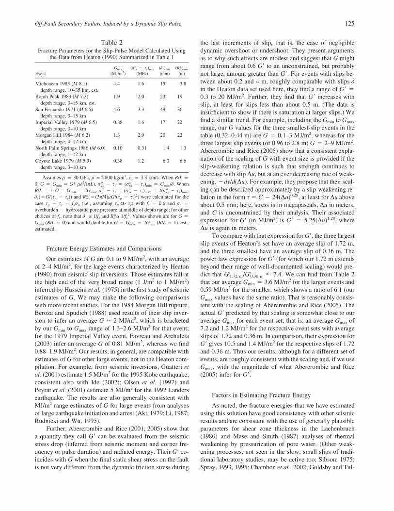
Table 2Fracture Parameters for the Slip-Pulse Model Calculated Using
the Data from Heaton (1990) Summarized in Table 1
EventGmin
(MJ/m2)( � sr)min
oryx
(MPa)(d1)min
(mm)( )minR*o
(m)
Michoacan 1985 (M 8.1) 4.4 1.6 15 3.8depth range, 10–35 km, est.
Borah Peak 1983 (M 7.3) 1.9 2.0 23 19depth range, 0–15 km, est.
San Fernando 1971 (M 6.5) 4.6 3.3 49 36depth range, 3–15 km
Imperial Valley 1979 (M 6.5) 0.88 1.6 17 22depth range, 0–10 km
Morgan Hill 1984 (M 6.2) 1.3 2.9 20 22depth range, 0–12 km
North Palm Springs 1986 (M 6.0) 0.10 0.31 1.4 1.3depth range, 1–12 km
Coyote Lake 1979 (M 5.9) 0.38 1.2 6.0 6.6depth range, 3–10 km
Assumes l � 30 GPa, q � 2800 kg/m3, cs � 3.3 km/s. When R/L �
0, G � Gmin � G* ld2/(pL), � sr � ( � sr)min � Gmin/d. Wheno or ryx yx
R/L � 1, G � Gmax � 2Gmin, � sr � ( � sr)max � 2( � sr)min.o o or r ryx yx yx
d1(�G/(sp � sr)) and (�(3p/4)lG/(sp � sr)2) were calculated for theR*o
case sp � sr � fs (i.e., assuming sp k sr) with fs � 0.6 and �r̄ r̄n n
overburden � hydrostatic pore pressure at middle of depth range; for otherchoices of fs, note that d1 � 1/fs and � 1/fs
2. Values shown are for G �R*oGmin (R/L � 0) and would double for G � Gmax � 2Gmin (R/L � 1). est.,estimated.
Fracture Energy Estimates and Comparisons
Our estimates of G are 0.1 to 9 MJ/m2, with an averageof 2–4 MJ/m2, for the large events characterized by Heaton(1990) from seismic slip inversions. Those estimates fall atthe high end of the very broad range (1 J/m2 to 1 MJ/m2)inferred by Husseini et al. (1975) in the first study of seismicestimates of G. We may make the following comparisonswith more recent studies. For the 1984 Morgan Hill rupture,Beroza and Spudich (1988) used results of their slip inver-sion to infer an average G � 2 MJ/m2, which is bracketedby our Gmin to Gmax range of 1.3–2.6 MJ/m2 for that event;for the 1979 Imperial Valley event, Favreau and Archuleta(2003) infer an average G of 0.81 MJ/m2, whereas we find0.88–1.9 MJ/m2. Our results, in general, are compatible withestimates of G for other large events, not in the Heaton com-pilation. For example, from seismic inversions, Guatteri etal. (2001) estimate 1.5 MJ/m2 for the 1995 Kobe earthquake,consistent also with Ide (2002); Olsen et al. (1997) andPeyrat et al. (2001) estimate 5 MJ/m2 for the 1992 Landersearthquake. The results are also generally consistent withMJ/m2 range estimates of G for large events from analysesof large earthquake initiation and arrest (Aki, 1979; Li, 1987;Rudnicki and Wu, 1995).
Further, Abercrombie and Rice (2001, 2005) show thata quantity they call G� can be evaluated from the seismicstress drop (inferred from seismic moment and corner fre-quency or pulse duration) and radiated energy. Their G� co-incides with G when the final static shear stress on the faultis not very different from the dynamic friction stress during
the last increments of slip, that is, the case of negligibledynamic overshoot or undershoot. They present argumentsas to why such effects are modest and suggest that G mightrange from about 0.6 G� to an unconstrained, but probablynot large, amount greater than G�. For events with slips be-tween about 0.2 and 4 m, roughly comparable with slips din the Heaton data set used here, they find a range of G� �0.3 to 20 MJ/m2. Further, they find that G� increases withslip, at least for slips less than about 0.5 m. (The data isinsufficient to show if there is saturation at larger slips.) Wefind a similar trend. For example, including the Gmin to Gmax
range, our G values for the three smallest-slip events in thetable (0.32–0.44 m) are G � 0.1–3 MJ/m2, whereas for thethree largest slip events (of 0.96 to 2.8 m) G � 2–9 MJ/m2.Abercrombie and Rice (2005) show that a consistent expla-nation of the scaling of G with event size is provided if theslip-weakening relation is such that strength continues todecrease with slip Du, but at an ever decreasing rate of weak-ening, �ds/d(Du). For example, they propose that their scal-ing can be described approximately by a slip-weakening re-lation in the form s � C � 24(Du)0.28, at least for Du aboveabout 0.5 mm; here, stress is in megapascals, Du in meters,and C is unconstrained by their analysis. Their associatedexpression for G� (in MJ/m2) is G� � 5.25(Du)1.28, whereDu is again in meters.
To compare with that expression for G�, the three largestslip events of Heaton’s set have an average slip of 1.72 m,and the three smallest have an average slip of 0.36 m. Thepower law expression for G� (for which our 1.72 m extendsbeyond their range of well-documented scaling) would pre-dict that G�1.72 m/G�0.36 m � 7.4. We can find from Table 2that our average Gmin � 3.6 MJ/m2 for the larger events and0.59 MJ/m2 for the smaller, which shows a ratio of 6.1 (ourGmax values have the same ratio). That is reasonably consis-tent with the scaling of Abercrombie and Rice (2005). Theactual G� predicted by that scaling is somewhat close to ouraverage Gmax for each event set; that is, an average Gmax of7.2 and 1.2 MJ/m2 for the respective event sets with averageslips of 1.72 and 0.36 m. In comparison, their expression forG� gives 10.5 and 1.4 MJ/m2 for the respective slips of 1.72and 0.36 m. Thus our results, although for a different set ofevents, are roughly consistent with the scaling and, if we useGmax, with the magnitude of what Abercrombie and Rice(2005) infer for G�.
Factors in Estimating Fracture Energy
As noted, the fracture energies that we have estimatedusing this solution have good consistency with other seismicresults and are consistent with the use of generally plausibleparameters for shear zone thickness in the Lachenbruch(1980) and Mase and Smith (1987) analyses of thermalweakening by pressurization of pore water. (Other weak-ening processes, not seen in the slow, small slips of tradi-tional laboratory studies, may be active too; Sibson, 1975;Spray, 1993, 1995; Chambon et al., 2002; Goldsby and Tul-

126 J. R. Rice, C. G. Sammis, and R. Parsons
lis, 2002.) However, a number of things could go wrong inmaking such seismic estimates of G as we do:
1. There are uncertainties in the seismic inversionsthemselves. For example, seismic records, in general, arefiltered in inversion studies at periods shorter than on theorder of 1 s, to remove effects of scattering; 1 s is the sameorder as the slip durations for most events listed in Table 1.
2. A correspondence of the mechanism leading to theapparently self-healing slip inferred in natural examples(Heaton, 1990) to the mechanism introduced in our modelcannot be confirmed. From the perspective of theoreticalmodels, self-healing is not a direct outcome of rupture mod-els like we consider with a slip-rate-independent frictionstress (Zheng and Rice, 1998); in general, it must be imposedin such models by propagating arrest phases or other inter-actions with heterogeneities (Day, 1982; Johnson, 1990; Per-rin et al., 1995; Beroza and Mikumo, 1996; Nielsen andCarlson, 2000; Nielsen and Madariaga, 2003). Self-healingcan also occur when spatially nonuniform slip can alter nor-mal stress across a fault plane, as for sliding between elas-tically dissimilar solids (Weertman, 1980; Andrews andBen-Zion, 1997; Harris and Day, 1997; Cochard and Rice,2000) or between certain foam rubbers (Brune et al., 1993).Such alteration of normal stress is, in principle, a genericconsequence of nonlinear constitutive response off the faultplane (Cochard and Rice, 2000), although such a route toself-healing pulses has not yet been demonstrated. Finally,slip-rate dependence of friction (Cochard and Madariaga,1994, 1996; Perrin et al., 1995; Beeler and Tullis, 1996;Nielsen and Carlson, 2000; Nielsen and Madariaga, 2003),at least if present under sufficiently low driving stress(Zheng and Rice, 1998), is a robust route to self-healing.Thus, the array of possible models for self-healing is greatand we do not have sufficiently general solutions, analogousto that developed here, for those other mechanisms to com-pare with the observations.
3. The constraint from slip inversions on rupture veloc-ity mr is actually a constraint on the average velocity. Wecannot rule out the possibility that there are very strong fluc-tuations in mr at periods shorter than those that can be re-solved in the inversion. In such cases we may argue that thenet energy flow G to the crack tip is sensibly estimated byour procedure, but only some of that (say, Gmat) is actuallydissipated in frictional processes near the rupture front andthe rest (call it Grad, so that G � Grad � Gmat) is radiatedout again from the crack tip as high-frequency stress waves.A simplified analysis of this effect (Rice, 2000) may be car-ried out in the context of a mode III singular crack (R/L r
0, scaled stress drop r 0). Let m�r be the time-variable in-stantaneous rupture speed, which averages to mr, and sup-pose, to make a simple tractable case, that m�r fluctuates rap-idly between two constant values
v̂ , very near c , for a fraction of the timer sv� �r �0 for the rest of the time.
This might roughly represent fracturing through a highlysegmented fault system in which the material energy ad-sorption Gmat is low on individual segments, so that getsv̂r
quite near cs, but rupture arrests at segment ends until stresswaves radiated out from there nucleate new ruptures onneighboring segments (e.g., Harris and Day, 1993).
During such rapidly fluctuating motion of the crack tipthat there is no energy flow per unit time to the crack tipwhen � 0, but there is an energy flow to inelastic pro-v�rcesses at the crack tip per unit time during the rapid motionat � , amounting tov� v̂r r
1 � v̂ /cr sG � Gmat rest�1 � v̂ /cr s
per unit fractured area (Eshelby, 1969a,b; Freund, 1990).Here, Grest is the “rest” value of the energy release rate andis unaffected by the rapid fluctuations (Rice et al., 1994;Morrissey and Rice, 1998). The G that we infer based onthe average speed mr must bear the same relation to Grest,namely,
1 � v /cr sG � G .rest�1 � v /cr s
By taking ratios and eliminating Grest, we thus find that thefraction of energy flow actually absorbed by inelastic pro-cesses at the tip is
G 1 � v̂ /c 1 � v /cmat r s r s� � �G 1 � v̂ /c 1 � v /cr s r s
and the remaining fraction (Grad/G � 1 � Gmat/G) is radi-ated out in the high-frequency wave field created by the rapidvelocity fluctuations. Thus, although we may with some con-fidence estimate G, that puts only an upper bound on howmuch energy is absorbed by the material near the tip, and inthis simple illustration Gmat may be made an arbitrarily smallfraction of G by making arbitrarily close to cs. For ex-v̂r
ample, if mr � 0.80cs and � 0.99cs, then Gmat � 0.21Gv̂r
and Grad � 0.79G.
Damage Zones and Fault Gouge
Although we used the PDR model primarily to explorefault branching, we can address the additional goal here ofexploring the mechanics responsible for the formation offragmented fault rock. The wall rocks of most faults areseparated by one or more layers of fragmented rock calledgouge or fault breccia. (See Ben-Zion and Sammis [2003]for a review of fault-zone structure.) Although there is con-siderable variation in the width of these layers and the extentof fragmentation within them, most faults with significantslip tend to have a structure described by Chester and Logan
Off-Fault Secondary Failure Induced by a Dynamic Slip Pulse 127
(1986, 1987), Chester et al. (1993), Evans and Chester(1995), Chester and Chester (1998), Schulz and Evans(2000), Lockner et al. (2000), Wibberley (2002), Wibberleyand Shimamoto (2003), and Otsuki et al. (2003). A “core”of extremely finely fragmented rock (possibly altered toclay) is bordered by layers of more coarsely fragmented faultbreccia. The core contains one or more planar surfaces whichappear to have accommodated most of the slip, and whichChester and Chester (1998) refer to as “prominent fracturesurfaces.” Somewhat surprisingly, the layers of fault brecciathat border the core appear to have accommodated little ifany strain, despite the fact that brecciation often extends tothe micron scale. Low strain is inferred from observationsthat relict structures from the host rock do not appear to besignificantly sheared.
Most studies of fault gouge and breccia to date havefocused on the particle-size distribution. Sammis et al.(1987) found that breccia from the Lopez Canyon Fault (abranch of the now extinct San Gabriel Fault in southern Cali-fornia) had a power law distribution of particle sizes consis-tent with a fractal structure. This was not the expected result,because existing fragmentation laws predicted either a log-normal or exponential Rosin-Ramler distribution (see, e.g.,Prasher, 1987). To explain these observations, Sammis et al.(1987) proposed a new fragmentation model, which theydubbed “constrained comminution.” In constrained commi-nution, particles are not free to move as they are in normalmilling operations. Rather, they are fixed in position relativeto other particles by the dense packing and high pressuresin the subterranean faulting environment. Consequently, theprobability of a particle fracturing is not dominated by itsfragility as in other fragmentation models, but by its loadinggeometry from adjacent particles. Particles loaded by same-sized neighbors have the highest fracture probability. Theprocess starts eliminating the largest (and hence weakest)particles until all large same-sized neighbors are eliminated,leaving isolated large particles cushioned by surroundingsmaller ones. The process then works its way down, elimi-nating smaller and smaller same-sized neighbors. The resultis a granular mass in which no two neighbors are the samesize at any scale. A fractal distribution having fractal di-mension D � 1.6 has this property; in fact, this is the fractaldimension found for the Lopez Canyon breccia. Constrainedcomminution has been observed in the double-shear frictionapparatus of J. H. Dieterich at U.S. Geological Survey (Bie-gel et al., 1989) and simulated in computer studies (Steacyand Sammis, 1991).
The development of a fractal particle distribution hasbeen shown to have important mechanical consequences.Biegel et al. (1989) found that the emergence of a fractaldistribution is closely associated with the observed transitionfrom velocity-strengthening friction (and stable sliding) tovelocity-weakening friction (and possible stick-slip instabil-ities). Sammis and Steacy (1994) proposed the explanationthat deformation in nonfractal distributions is accommo-dated mostly by the failure of particles which, as in triaxial
laboratory experiments, is velocity strengthening. As a frac-tal distribution is developed it becomes increasingly difficultto fracture particles and, at the same time, reduced dilatationsignals that it is easier to accommodate deformation by slipbetween particles. Because the resistance to slip increaseswith the age of the particle contacts, velocity weakeningbecomes possible and the macroscopic friction transitionsfrom velocity strengthening associated with the fracture ofparticles to weakening associated with slip between them.
The reduced dilatation associated with the evolvingfractal distribution also leads to shear localization on sur-faces within the granular mass. From this perspective, thereason fault breccia has low strain is that it represents onlythe initial phase of fault formation. Breccia forms early in afault’s history as it grows by linking offset strands (Segalland Pollard, 1983) and removing geometric asperities(Power et al., 1988). If these asperities have a fractal sizedistribution (i.e., the fault surface has fractal roughness),Power et al. (1988) show that the scale of the geometricalmismatch grows with fault displacement in such a way thatthe thickness of the resultant gouge and breccia zone in-creases approximately linearly with displacement, as oftenobserved (Scholz, 1987; Hull, 1988). However, only a rela-tively small strain on the order of about 3 is required toproduce a fractal gouge (Biegel et al., 1989), after whichstrain localizes onto a prominent slip surface. Once strainhas localized, the gouge layer is a relict structure playing nosignificant role in the accommodation of additional strain.
This view of the formation and mechanical significanceof gouge has recently been challenged by Brune (2001), whoproposed that fault breccia is formed by dynamic stresschanges during an earthquake. In particular, he argues thatgouge forms during the dynamic reduction of normal stressacross a fault accompanying the propagation of a “wrinklepulse,” or dynamic pore pressure reduction, or any otheropening type motion of the class recently proposed to allowfaulting without the attendant generation of heat—thus solv-ing the “heat-flow paradox” for the San Andreas fault. Asevidence, Brune cites the apparent lack of significant strain,observations of “exploded grains” that have obviously failedin tension, and the orientation of small slip surfaces withinthe breccia that are aligned at high angles to the prominentslip surface. As mentioned previously, the apparent lack ofstrain is not unique to dynamic rupture. Nor is the obser-vation of grains that have failed in tension since such grainswere observed in double-shear friction experiments (Biegelet al., 1989) where all macroscopic stresses were compres-sive. Tensile failure in that case resulted from the failure ofindividual grains under bipolar loading by same-sized neigh-bors in the load-bearing ligands (stress chains) that transmitforce in granular media. It should be noted that Brune’s hy-pothesis is consistent with Sibson’s (1986) observation that“explosion breccia” tends to form in dilatational fault jogs.However, this is an expected outcome in quasistatic defor-mation and does not require a dynamic opening-type modeof rupture.
128 J. R. Rice, C. G. Sammis, and R. Parsons
Our results show that the dynamic stress field from apropagating slip pulse can produce Coulomb slip on preex-isting fractures which extends out to a scaled distance on theorder of 1–2 in the range of typical seismic rupture ve-R*olocities, mr � 0.7–0.9cs. Using our model to analyze the slippulses observed by Heaton (1990) for seven large events,we found that is in the range of 1 to 40 m if sp � sr �R*o0.6 , and can be on the order of kilometers if the strengthr̄n
drop is low, for example, (sp � sr) � 10 MPa. These resultsare roughly consistent with observations by Wilson et al.(1999) that a zone of oriented microfracture damage extendsto distances of about 30 m from the exhumed PunchbowlFault in southern California, and that random microfracturesare above the background level to distances of about 100 m.
Coulomb slip on preexisting fractures is a necessary, butnot sufficient, condition for compressive failure and frag-mentation of crystalline rock. A damage mechanics analysis(such as Ashby and Sammis, 1990) is required to map theboundaries of fragmentation. However, under certain con-ditions, we found that the minimum principal stress r2 be-comes positive (tensile), which would almost certainly pro-duce failure and fragmentation. As is evident in Figure 5,tensile stress is favored by a preexisting maximum com-pression direction at a high angle w to the fault plane, anda high value of the rupture velocity mr. The extent to whichthe fault zone becomes narrower with depth depends on thedepth dependence of d1/(sp � sr). If (sp � sr) depends onthe effective normal stress through a coefficient of friction,then the zone width should decrease linearly with depth.
Acknowledgments
This study was supported by NSF-EAR Awards 0105344 and0125709 to Harvard, by NSF-EAR Award 9902901 to USC, and by theNSF/USGS Southern California Earthquake Center (SCEC). SCEC is sup-ported through USGS cooperative agreement 02HQAG0008 and NSF co-operative agreement EAR-0106924. This is SCEC Contribution Number732. We are grateful to J. W. Rudnicki for helping us improve the presen-tation, and for reviews by T. H. Heaton and R. Madariaga.
References
Abercrombie, R. E., and J. R. Rice (2001). Small earthquake scaling revis-ited: can it constrain slip weakening? (abstract), EOS Trans. Am. Geo-phys. Union 82, no. 47 (Fall Meeting Suppl.), S21E-04, F843.
Abercrombie, R. E., and J. R. Rice (2005). Can observations of earthquakescaling constrain slip weakening? Geophys. J. Int. (in press).
Aki, K. (1979). Characterization of barriers on an earthquake fault, J. Geo-phys. Res. 84, 6140–6148.
Aki, K., and P. G. Richards (1980). Quantitative Seismology: Theory andMethods, Freeman, New York.
Andrews, D. J. (1976a). Rupture propagation with finite stress in antiplanestrain, J. Geophys. Res. 81, 3575–3582.
Andrews, D. J. (1976b). Rupture velocity of plane strain shear cracks, J.Geophys. Res. 81, 5679–5687.
Andrews, D. J. (2003). A fault constitutive relation accounting for thermalpressurization of pore fluid, J. Geophys. Res. 107, (no. B12), 2363,doi 10.1029/2002JB001942.
Andrews, D. J., and Y. Ben-Zion (1997). Wrinkle-like slip pulse on a faultbetween different materials, J. Geophys. Res. 102, 553–571.
Ashby, M. F., and C. G. Sammis (1990). The damage mechanics of brittlesolids in compression, Pure Appl. Geophys. 133, 489–521.
Beeler, N. M., and T. E. Tullis (1996). Self-healing slip pulse in dynamicrupture models due to velocity-dependent strength, Bull. Seism Soc.Am. 86, 1130–1148.
Ben-Zion, Y., and C. G. Sammis (2003). Characterization of fault zones,Pure Appl. Geophys. 160, 677–715.
Beroza, G. C., and T. Mikumo (1996). Short slip duration in dynamic rup-ture in the presence of heterogeneous fault properties, J. Geophys.Res. 101, 22,449–22,460.
Beroza, G. C., and P. Spudich (1988). Linearized inversion for fault rupturebehavior: application to the 1984 Morgan Hill, California, earthquake,J. Geophys. Res. 93, 6275–6296.
Biegel, R. L., C. G. Sammis, and J. H. Dieterich (1989). The frictionalproperties of a simulated gouge having a fractal particle distribution,J. Structural Geol. 11, 827–846.
Broberg, K. B. (1978). On transient sliding motion, Geophys. J. R. Astr.Soc. 52, 397–432.
Broberg, K. B. (1999). Cracks and Fracture, Academic Press, San Diego.Brune, J. N. (2001). Fault-normal dynamic unloading and loading: an ex-
planation for “non-gouge” rock powder and lack of fault-parallelshear bands along the San Andreas fault (abstract), EOS Trans. Am.Geophys. Union 82, no. 47 (Fall Meeting Suppl.), F854.
Brune, J. N., S. Brown, and P. A. Johnson (1993). Rupture mechanism andinterface separation in foam rubber models of earthquakes: a possiblesolution to the heat flow paradox and the paradox of large overthrusts,Tectonophysics 218, 59–67.
Chambon, G., J. Schmittbuhl, and A Corfdir (2002). Laboratory gougefriction: seismic-like slip weakening and secondary rate- and state-effects, Geophys. Res. Lett. 29, no. 10, doi 10.1029/2001GL014467.
Chester, F. M., and J. M. Logan (1986). Implications for mechanical prop-erties of brittle faults from observations of the Punchbowl fault zone,California, Pure Appl. Geophys. 124, 79–106.
Chester, F. M., and J. M. Logan (1987). Composite planar fabric of gougefrom the Punchbowl fault, California, J. Struct. Geol. 9, 621–634.
Chester, F. M., and J. S. Chester (1998). Ultracataclasite structure and fric-tion processes of the Punchbowl fault, San Andreas system, Califor-nia, Tectonophysics 295, 199–221.
Chester, F. M., J. P. Evans, and R. L. Biegel (1993). Internal structure andweakening mechanisms of the San Andreas fault, J. Geophys. Res.98, 771–786.
Cochard, A., and R. Madariaga (1994). Dynamic faulting under rate-de-pendent friction, Pure Appl. Geophys. 142, 419–445.
Cochard, A., and R. Madariaga (1996). Complexity of seismicity due tohighly rate dependent friction, J. Geophys. Res. 101, no. B11, 25,321–25,336.
Cochard, A., and J. R. Rice (2000). Fault rupture between dissimilar ma-terials: Ill-posedness, regularization, and slip-pulse response, J. Geo-phys. Res. 105, no. B11, 25,891–25,907.
Day, S. M. (1982). Three-dimensional finite difference simulation of faultdynamics: rectangular faults with fixed rupture velocity, Bull. Seism.Soc. Am. 72, 705–727.
Erdogan, F. (1968). Crack-propagation theories, in Fracture: An AdvancedTreatise, H. Liebowitz (Editor), Vol. 2. Mathematical Fundamentals,Academic Press, New York, 497–590.
Eshelby, J. D. (1969a). The elastic field of a crack extending non-uniformlyunder general anti-plane loading, J. Mech. Phys. Solids 17, 177.
Eshelby, J. D. (1969b). The starting of a crack, in Physics of Strength andPlasticity, A. S. Argon (Editor), The MIT Press, Cambridge, Massa-chusetts, 263–275.
Evans, J. P., and F. M. Chester (1995). Fluid-rock interaction in faults ofthe San Andreas system: Inferences from San Gabriel fault rock geo-chemistry and microstructures, J. Geophys. Res. 100, 13,007–13,020.
Favreau, P., and R. J. Archuleta (2003). Direct seismic energy modelingand application to the 1979 Imperial Valley earthquake, Geophys.Res. Lett. 30, no 5, 1198, doi 10.1029/2002GL015968.
Off-Fault Secondary Failure Induced by a Dynamic Slip Pulse 129
Freund, L. B. (1979). The mechanics of dynamic shear crack propagation,J. Geophys. Res. 84, 2199–2209.
Freund, L. B. (1990). Dynamic Fracture Mechanics, Cambridge Univ.Press, Cambridge.
Goldsby, D. L., and T. E. Tullis (2002). Low frictional strength of quartzrocks at subseismic slip rates, Geophys. Res., Lett. 29, no. 17, 1844,doi 10.1029/2002GL015240.
Guatteri, M., P. Spudich, and G. C. Beroza (2001). Inferring rate and statefriction parameters from rupture models of the 1995 Hyogo-kenNambu (Kobe) earthquake, J. Geophys. Res. 106, no. B11, 26,511–26,521.
Harris, R., and S. M. Day (1993). Dynamics of fault interactions: parallelstrike-slip faults, J. Geophys. Res. 98, 4461–4472.
Harris, R., and S. M. Day (1997). Effects of a low velocity zone on adynamic rupture, Bull. Seism. Soc. Am. 87, 1267–1280.
Heaton, T. H. (1990). Evidence for and implications of self-healing pulsesof slip in earthquake rupture, Earth Planet. Int. 64, 1–20.
Hull, J. (1988). Thickness-displacement relationships for deformationzones, J. Struct. Geol. 10, 431–435.
Husseini, M. I., D. B. Jovanovich, M. J. Randall, and L. B. Freund (1975).The fracture energy of earthquakes, Geophys. J. R. Astr. Soc. 43,367–385.
Ida, Y. (1972). Cohesive force across the tip of a longitudinal shear crackand Griffith’s crack specific surface energy, J. Geophys. Res. 77,3796–3805.
Ide, S. (2002). Estimation of radiated energy of finite-source earthquakemodels, Bull. Seism. Soc. Am. 92, no. 8, 2994–3005.
Johnson, E. (1990). On the initiation of unidirectional slip, Geophys. J. Int.101, 125–132.
Kame, N., and T. Yamashita (1999). Simulation of the spontaneous growthof a dynamic crack without constraints on the crack tip path, Geophys.J. Int. 139, 345–358.
Kame, N., J. R. Rice, and R. Dmowska (2003). Effects of pre-stress andrupture velocity on dynamic fault branching, J. Geophys. Res. 108,no. B5, 2265, doi 10.1029/2002JB002189, ESE 13-1–13-21.
Lachenbruch, A. H. (1980). Frictional heating, fluid pressure, and the re-sistance to fault motion, J. Geophys. Res. 85, 6097–6112.
Lachenbruch, A. H., and J. H. Sass (1980). Heat flow and energetics of theSan Andreas fault zone, J. Geophys. Res. 85, 6185–6222.
Li, V. C. (1987). Mechanics of shear rupture applied to earthquake zones,Fracture Mechanics of Rock, B. K. Atkinson (Editor), AcademicPress, London, 351–428.
Lockner, D., H. Naka, H. Tanaka, H. Ito, and R. Ikeda (2000). Permeabilityand strength of core samples from the Nojima fault of the 1995 Kobeearthquake, in Proceedings of the Internaional Workshop on the No-jima Fault Core and Borehole Data Analysis, Tsukuba, Japan, 22–23, November 1999, H. Ito, K. Fujimoto, H. Tanaka, and D. Lockner(Editors), U.S. Geol. Surv. Open-File Rept. 00-129, 147–152.
Mase, C. W., and L. Smith (1987). Effects of frictional heating on thethermal, hydrologic, and mechanical response of a fault, J. Geophys.Res. 92, 6249–6272.
Morrissey, J. W., and J. R. Rice (1998), Crack front waves, J. Mech. Phys.Solids 46, 467–487.
Muskhelishvili, N. I. (trans. by J. R. M. Radok) (1953). Some Basic Prob-lems of the Mathematical Theory of Elasticity, Noordhoff, Groningen.
Nielsen, S. B., and J. M. Carlson (2000). Rupture pulse characterization;self-healing, self-similar, expanding solutions in a continuum modelof fault dynamics, Bull. Seism. Soc. Am. 90, 1480–1497.
Nielsen, S., and R. Madariaga (2003). On the self-healing fracture mode,Bull. Seism. Soc. Am. 93, no. 6, 2375–2388.
Olsen, K., R. Madariaga, and R. Archuleta (1997). Three dimensional dy-namic simulation of the 1992 Landers earthquake, Science 278,834–838.
Otsuki, K., N. Monzawa, and T. Nagase (2003). Fluidization and meltingof fault gouge during seismic slip: identification in the Nojima faultzone and implications for local earthquake mechanisms, J. Geophys.Res. 108, no. B4, 2192, doi 10.1029/2001JB001711, ESE 4-1–4-18.
Palmer, A. C., and J. R. Rice (1973). The growth of slip surfaces in theprogressive failure of over-consolidated clay, Proc. R. Soc. LondonA 322, 527–548.
Perrin, G., J. R. Rice, and G. Zheng (1995). Self-healing slip pulse on africtional surface, J. Mech. Phys. Solids 43, 1461–1495.
Peyrat, S., K. Olsen, and R. Madariaga (2001). Dynamic modeling of the1992 Landers earthquake, J. Geophys. Res. 106, no. B11, 26,467–26,482.
Poliakov, A. N. B., R. Dmowska, and J. R. Rice (2002). Dynamic shearrupture interactions with fault bends and off-axis secondary faulting,J. Geophys. Res. 107, no. B11, 2295, doi 10.1029/2001JB000572,ESE 6-1–6-18.
Pollard, D. D., and P. Segall (1987). Theoretical displacements and stressesnear fractures in rock: with applications to faults, joints, veins, dikes,and solution surfaces, in Fracture Mechanics of Rock, B. K. Atkinson(Editor), Academic Press, London, 277–349.
Power, W. L., T. E. Tullis, and J. D. Weeks (1988). Roughness and wearduring brittle faulting, J. Geophys. Res. 93, 15,268–15,278.
Prasher, C. (1987). Crushing and Grinding Process Handbook, John Wileyand Sons, New York.
Rice, J. R. (1980). The mechanics of earthquake rupture, in Physics of theEarth’s Interior, Proc. International School of Physics ‘Enrico Fermi’,A. M. Dziewonski and E. Boschi (Editors), Italian Physical Society,Bologna, and North Holland Publishing Co., Amsterdam, 555–649.
Rice, J. R. (1999). Flash heating at asperity contacts and rate-dependentfriction (abstract), EOS Trans. Am. Geophys. Union 80, no. 46 (FallMeet. Suppl.), F681.
Rice, J. R. (2000). Fracture energy of earthquakes and slip-weakening rup-ture parameters (abstract), EOS Trans. Am. Geophys. Union 81 (FallMeet. Suppl.), F1227.
Rice, J. R. (2003). Earthquake fracture energies and weakening of faultsby thermal pressurization of pore fluid (abstract), EOS Trans. Am.Geophys. Union 84 (Fall Meet. Suppl.), S41G-01, F1088.
Rice, J. R., and M. P. Cleary (1976). Some basic stress-diffusion solutionsfor fluid-saturated elastic porous media with compressible constitu-ents, Rev. Geophys. Space Phys. 14, 227–241.
Rice, J. R., Y. Ben-Zion, and K. S. Kim (1994), Three-dimensional per-turbation solution for a dynamic planar crack moving unsteadily in amodel elastic solid, J. Mech. Phys. Solids 42, 813–843.
Rubin, A. M., and C. B. Parker (1994). Near-tip stress fields for dynami-cally propagating mode-II fractures, in The Mechanical Involvementof Fluids in Faulting, S. Hickman, R. Sibson, and R. Bruhn (Editors),U.S. Geol. Surv. Open-File Rept. 94-228, 399–405.
Rudnicki, J. W., and M. Wu (1995). Mechanics of dip-slip faulting in anelastic half-space, J. Geophys Res. 100, no. B11, 22,173–22,186.
Sammis, C.G., and S. J. Steacy (1994). The micromechanics of friction ina granular layer, Pure Appl. Geophys. 142, 777–794.
Sammis, C. G., G. C. P. King, and R. Biegel (1987). The kinematics ofgouge deformation, Pure Appl. Geophys. 125, 777–812.
Scholz, C. H. (1987). Wear and gouge formation in brittle faulting, Geology15, 493–495.
Schulz, S. E., and J. P. Evans (2000). Mesoscopic structure of the Punch-bowl fault, southern California and the geologic and geophysicalstructure of active strike slip faults, J. Struct. Geol. 22, 913–930.
Segall, P., and D. D. Pollard (1980). Mechanics of discontinuous faults,J. Geophys. Res. 85, 4337–4350.
Segall, P., and D. D. Pollard (1983). Nucleation and growth of strike-slipfaults in granite, J. Geophys. Res. 88, 555–568.
Segall, P., and J. R. Rice (1995). Dilatancy, compaction, and slip instabilityof a fluid infiltrated fault, J. Geophys. Res. 100, 22,155–22,171.
Sibson, R. H. (1973). Interactions between temperature and pore-fluid pres-sure during earthquake faulting and a mechanism for partial or totalstress relief, Nature 243, no. 126, 66–68.
Sibson, R. H. (1975). Generation of pseudotachylyte by ancient seismicfaulting, Geophys. J. R. Astr. Soc. 43, 775–794.
Sibson, R. H. (1986). Brecciation processes in fault zones: inferences fromearthquake rupturing, Pure Appl. Geophys. 124, 159–176.

130 J. R. Rice, C. G. Sammis, and R. Parsons
Spray, J. G. (1993). Viscosity determinations of some frictionally generatedsilicate melts; implications for fault zone rheology at high strain rates,J. Geophys. Res. 98, 8053–8068.
Spray, J. G. (1995). Pseudotachylyte controversy; fact or friction?, Geology23, 1119–1122.
Steacy, S. J., and C. G. Sammis (1991). An automaton for fractal patternsof fragmentation, Nature 353, 250–252.
Tullis, T. E., and D. Goldsby (2003), Flash melting of crustal rocks atalmost seismic slip rates (abstract), EOS Trans. Am. Geophys. Union84, no. 46 (Fall Meet. Suppl.), S51B-05, F1114.
Weertman, J. (1980). Unstable slippage across a fault that separates elasticmedia of different elastic-constants, J. Geophys. Res. 85, no. B3,1455–1461.
Wibberley, C. A. J. (2002). Hydraulic diffusivity of fault gouge zones andimplications for thermal pressurization during seismic slip, EarthPlanets Space 54, no. 11, 1153–1171.
Wibberley, C. A. J., and T. Shimamoto T. (2003). Internal structure andpermeability of major strike-slip fault zones: the Median TectonicLine in Mie Prefecture, Southwest Japan, J. Struct. Geol. 25, 59–78.
Wilson, J. E., J. S. Chester, and F. M. Chester (1999). Microfracture fabricof the Punchbowl Fault zone, San Andreas system, California, EOSTrans. Am. Geophys. Union 81, (Fall Meeting Suppl.), F746–F747.
Yoffe, E. H. (1951). The moving Griffith crack, Phil. Mag. 42, 739–750.Zheng, G., and J. R. Rice (1998). Conditions under which velocity-weak-
ening friction allows a self-healing versus a cracklike mode of rupture,Bull. Seism. Soc. Am. 88, 1466–1483.
Zoback, M. D., M. L. Zoback, V. S. Mount, J. Suppe, J. P. Eaton, J. H.Healy, D. Oppenheimer, P. Reasenberg, L. Jones, C. B. Raleigh, I. G.Wong, O. Scotti, and C. Wentworth (1988). New evidence on thestate of stress of the San Andreas fault system, Science 238, 1105–1111.
Appendix: Stresses Near a Propagating Slip Pulse
This appendix is an extension of the appendix in Polia-kov et al. (2002) (PDR) to the case of a finite sliding zone,as considered earlier by Broberg (1978) and Freund (1979).The analysis is done here for the particular slip-weakeningmodel illustrated in Figure 2. The problem is again to findan analytic function M(z) of the complex variable z, this timehaving a specified stress on the slipping portion of the x axis�L � x � 0.
For mode II
or � r � Re[M(x)] on �L � x � 0, (A1)yx yx
and, as discussed in the text, we require
Re[M(x)]os � r , �L � x � �Rr yx
� x o� 1 � (s � s ) � s � r , �R � x � 0p r r yx� �R(A2)
For mode III, substitute for .o or ryz yx
Additional conditions imposed are that M(z) vanishes asz r � and is bounded as z r 0 and as z r �L. Note that inour problem, because ryx and ryz are continuous across thefault,
� �Re[M (x)] � Re[M (x)] � g(x) (A3)
for �� � x � �, where g(x) is the right side in (A2) for�L � x � 0 and is ryx(x,0) � for all x.oryx
If we define M̄(f) as , then M̄(z̄) � , and¯M(f) M(z)2Re[M(z)] � M(z) � M̄(z̄). Hence, 2Re[M�(x)] � M�(x)� M̄�(x) � 2Re[M�(x)] � M�(x) � M̄�(x) � 2g(x), andwe find by subtraction that [M(x) � M̄(x)]� � [M(x) �M̄(x)]� for all x. This means that M(z) � M̄(z) is actuallyanalytic across the cut, and hence is analytic everywhere.But M(z) r 0 and M̄(z) r 0 as |z| r �. Thus, M(z) � M̄(z)� 0 for all z, which means that M̄(z) � M(z) and 2Re[M(z)]� M(z) � M(z̄). Thus, Re[M(x)] � g(x), �L � x � 0, isequivalent to the condition
� �M (x) � M (x) � 2g(x), �L � x � 0. (A4)
By standard methods (e.g., Muskhelishvili, 1953) wenow seek a function X(z), which is analytic outside the cutand satisfies X�(x) � X�(x) � 0, �L � x � 0, so thatwhen we divide (A4) by X�(x) and use X�(x) � �X�(x),we get
� �M(x) M(x) 2g(x)� � (A5)� � � � �X(x) X(x) X (x)
on the cut. We note also that M(z)/X(z) is also analytic out-side the cut if X(z) has no zeros there.
Such a function that satisfies X� (x) � X� (x) � 0 isX(z) � z�1/2 (z � L)�1/2, where z1/2 � , with z �ih /21r e� 1
and �p � h1 � �p, and (z � L)1/2 � , withih ih /21 2r e r e�1 2
z � L � r2eih2 and �p � h2 � �p.The motivation for this transformation is that (A5) is in
a suitable form to solve with the Cauchy integral represen-tation. Letting F(z) � M(z)/X(z) and h(x) � 2g(x)/X�(x),we have the problem of finding the function F(z), analyticoutside the cut from �L to 0, and constant at � (because itis easy to show that our M(z) is such that zM(z) remainsbounded as z r �), satisfying F�(x) � F�(x) � h(x), agiven function on �L � x � 0. Referring to Figure A1, theCauchy integral representation is
F(t) F(t)2piF(z) � � dt � � dt
t� z t� zC Cq cut
where Ccut is traversed in clockwise sense and Cq (a largecircle of radius q) in counter-clockwise sense, shrinking Ccut
to the slipping zone along the x axis:
� �0 0F(t) F (t) � F (t) h(t)� dt � dt � dt . t� z �L t� z �L t� zCcut
Letting q r �
F(t) dtlim � dt � F(�) � � 2piF(�)
t� z tqr� C CR R
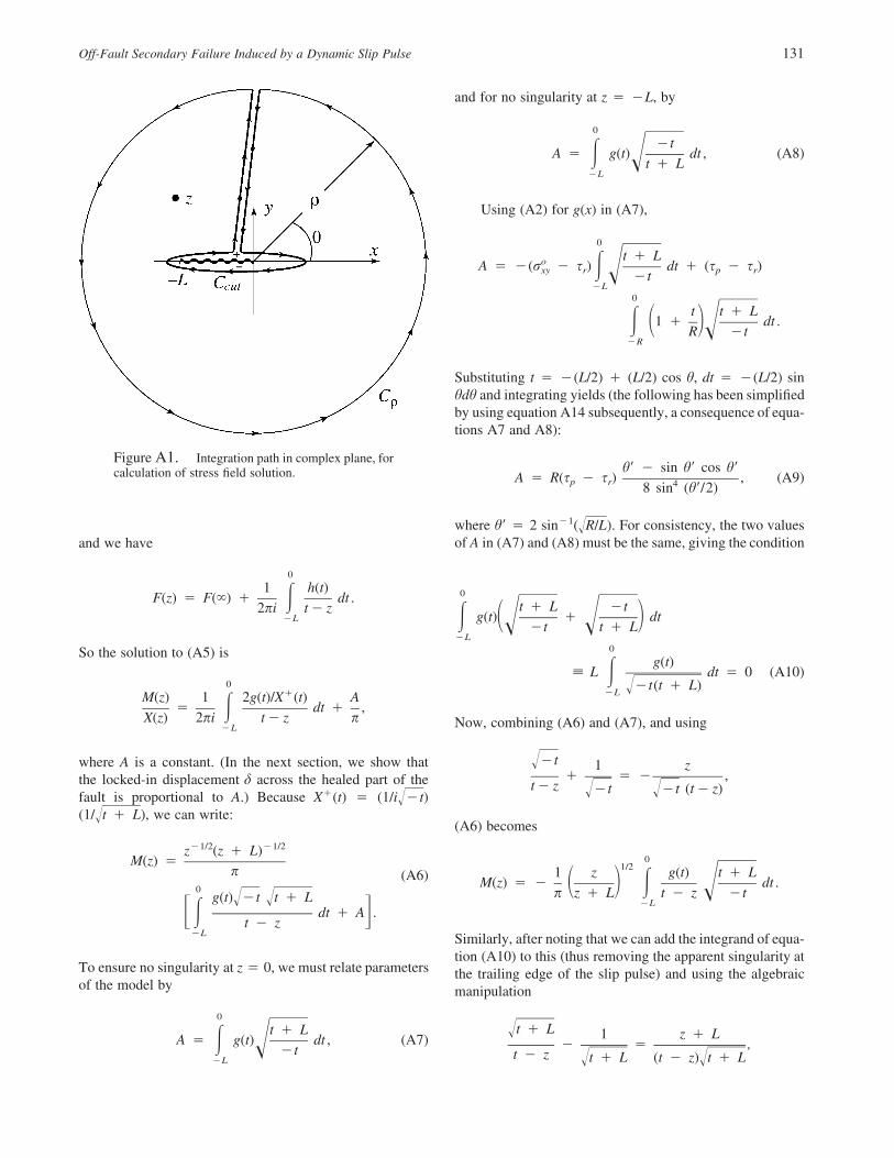
Off-Fault Secondary Failure Induced by a Dynamic Slip Pulse 131
Figure A1. Integration path in complex plane, forcalculation of stress field solution.
and we have
0
1 h(t)F(z) � F(�) � dt .2pi t� z
�L
So the solution to (A5) is
0�M(z) 1 2g(t)/X (t) A
� dt � ,X(z) 2pi t� z p�L
where A is a constant. (In the next section, we show thatthe locked-in displacement d across the healed part of thefault is proportional to A.) Because X�(t) � (1/i �t)�
, we can write:(1/ t � L)�
�1/2 �1/2z (z � L)M(z) �
p (A6)0
g(t) �t t � L� �dt � A .� �t � z
�L
To ensure no singularity at z � 0, we must relate parametersof the model by
0
t � LA � g(t) dt , (A7) � �t
�L
and for no singularity at z � �L, by
0
�tA � g(t) dt , (A8) �t � L
�L
Using (A2) for g(x) in (A7),
0
t � LoA � �(r � s ) dt � (s � s )xy r p r� �t�L
0
t t � L1 � dt . � ��R �t
�R
Substituting t � �(L/2) � (L/2) cos h, dt � �(L/2) sinhdh and integrating yields (the following has been simplifiedby using equation A14 subsequently, a consequence of equa-tions A7 and A8):
h� � sin h� cos h�A � R(s � s ) , (A9)p r 48 sin (h�/2)
where h� � 2 sin�1( ). For consistency, the two valuesR/L�of A in (A7) and (A8) must be the same, giving the condition
0
t � L �tg(t) � dt � �� ��t t � L
�L0
g(t)� L dt � 0 (A10)
�t(t � L)��L
Now, combining (A6) and (A7), and using
�t� 1 z� � � ,
t� z �t �t (t� z)� �
(A6) becomes
01/21 z g(t) t � L
M(z) � � dt .� � �p z � L t � z �t�L
Similarly, after noting that we can add the integrand of equa-tion (A10) to this (thus removing the apparent singularity atthe trailing edge of the slip pulse) and using the algebraicmanipulation
t � L� 1 z � L� � ,
t � z t � L (t � z) t � L� �
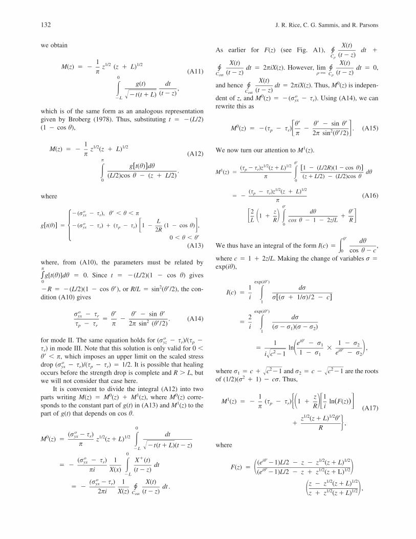
132 J. R. Rice, C. G. Sammis, and R. Parsons
we obtain
1 1/2 1/2M(z) � � z (z � L)p (A11)
0
g(t) dt, (t� z)�t(t�L)��L
which is of the same form as an analogous representationgiven by Broberg (1978). Thus, substituting t � �(L/2)(1 � cos h),
1 1/2 1/2M(z) � � z (z � L)p (A12)
p
g[t(h)]dh. (L/2)cos h � (z � L/2)
0
where
o�(r � s ), h� � h � pyx r
Log[t(h)] � �(r � s ) � (s � s ) 1 � (1 � cos h) ,yx r p r � �2R�0 � h � h�
(A13)
where, from (A10), the parameters must be related by
g[t(h)]dh � 0. Since t � �(L/2)(1 � cos h) givesp
�0
�R � �(L/2)(1 � cos h�), or R/L � sin2(h�/2), the con-dition (A10) gives
or � s h� h� � sin h�yx r� � . (A14)2s � s p 2p sin (h�/2)p r
for mode II. The same equation holds for ( � sr)/(sp �oryz
sr) in mode III. Note that this solution is only valid for 0 �h� � p, which imposes an upper limit on the scaled stressdrop ( � sr)/(sp � sr) � 1/2. It is possible that healingoryx
occurs before the strength drop is complete and R � L, butwe will not consider that case here.
It is convenient to divide the integral (A12) into twoparts writing M(z) � M0(z) � M1(z), where M0(z) corre-sponds to the constant part of g(t) in (A13) and M1(z) to thepart of g(t) that depends on cos h.
0o(r �s ) dtyx r0 1/2 1/2M (z) � z (z�L) p �t(t�L)(t� z)��L
0o �(r � s ) 1 X (t)yx r
� � dtpi X(x) (t� z)�L
o(r �s ) 1 X(t)yx r� � � dt .
2pi X(z) (t� z)Ccut
As earlier for F(z) (see Fig. A1), dt �X(t)
�(t� z)Cq
dt � 2piX(z). However, dt � 0,X(t) X(t)
� lim �(t� z) qr� (t� z)C Ccut q
and hence dt � 2piX(z). Thus, M0(z) is indepen-X(t)
�(t� z)Ccut
dent of z, and M0(z) � �( � sr). Using (A14), we canoryx
rewrite this as
h� h� � sin h�0M (z) � �(s � s ) � . (A15)p r � 2 �p 2p sin (h�/2)
We now turn our attention to M1(z).
h�1/2 1/2(s �s )z (z�L) [1 � (L/2R)(1�cos h)]p r1M (z) � dhp (z�L/2) � (L/2)cos h
0
1/2 1/2(s � s )z (z � L)p r� � (A16)
ph�
2 z dh h�1 � �� � � �L R cos h � 1 � 2z/L R
0
We thus have an integral of the form I(c) � ,h� dh
0 cos h�cwhere c � 1 � 2z/L. Making the change of variables r �exp(ih),
exp(ih�)
1 drI(c) � i r[(r � 1/r)/2 � c]
1
exp(ih�)
2 dr� i (r�r )(r�r )1 2
1
ih�1 e � r 1 � r1 2� ln � ,� ih� �2 1 � r e � r1 2i c �1�
where r1 � c � and r2 � c � are the roots2 2c �1 c �1� �of (1/2)(r2 � 1) � cr. Thus,
1 z 11M (z) � � (s � s ) 1 � ln(F(z))p r �� �� �p R i (A17)1/2 1/2z (z�L) h�
� ,�R
where
ih� 1/2 1/2(e �1)L/2 � z � z (z�L)F(z) � � ih� 1/2 1/2�(e �1)L/2 � z � z (z�L)
1/2 1/2z � z (z�L),� 1/2 1/2�z � z (z�L)
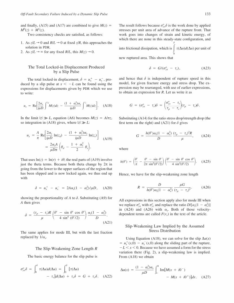
Off-Fault Secondary Failure Induced by a Dynamic Slip Pulse 133
and finally, (A15) and (A17) are combined to give M(z) �M0(z) � M1(z).
Two consistency checks are satisfied, as follows:
1. As z/L r 0 and R/L r 0 at fixed z/R, this approaches thesolution in PDR.
2. As z/L r � for any fixed R/L, this M(z) r 0.
The Total Locked-in Displacement Producedby a Slip Pulse
The total locked-in displacement, d � � , pro-� �u ux x
duced by a slip pulse at x � �L can be found using theexpressions for displacements given by PDR which we useto write:
2z zd s2� (1 � � )�s s su � Re M(z)dz � M(z)dz . (A18)x � �ilD ilD
In the limit |z| k L, equation (A6) becomes M(z) � A/pz,so integration in (A18) gives, where |z| k L:
2A 2� (1 � � )�s s su � Re ln(z ) � ln(z )x d s� �p ilD ilD (A19)22� A 1 � �s s
� h � h .d s� �lDp 2
That uses ln(z) � ln(r) � ih; the real parts of (A19) involvejust the theta terms. Because both theta change by 2p ingoing from the lower to the upper surfaces of the region thathas been slipped and is now locked again, we thus end upwith
� � 2d � u � u � 2A� (1 � � ) /lD , (A20)x x s s
showing the proportionality of A to d. Substituting (A9) forA then gives
2(s � s )R h� � sin h� cos h� � (1 � � )p r s sd � .� 4 �l 4 sin (h�/2) D
(A21)
The same applies for mode III, but with the last fractionreplaced by 1/�s.
The Slip-Weakening Zone Length R
The basic energy balance for the slip pulse is
d dor d � s(Du)d(Du) � [s(Du)yx
0 0
� s ]d(Du) � s d � G � s d . (A22)r r r
The result follows because is the work done by appliedor dyx
stresses per unit area of advance of the rupture front. Thatwork goes into changes of strain and kinetic energy, ofwhich there are none in this steady-state configuration, and
into frictional dissipation, which is s(Du)d(Du) per unit of
d
0
new ruptured area. This shows that
od � G/(r � s ) , (A23)yx r
and hence that d is independent of rupture speed in thismodel, for given fracture energy and stress drop. The ex-pression may be rearranged, with use of earlier expressions,to obtain an expression for R. Let us write it as
or � syx roG � (r � s )d � (s � s )d .yx r p r� �s � sp r
Substituting (A14) for the ratio stress drop/strength drop (thefirst term on the right) and (A21) for d gives
2 2h(h�)� (1 � � ) (s � s ) Rs s p rG � , (A24)D l
where
h� h� � sin h� h� � sin h� cos h�h(h�) � � . (A25)� 2 � � 4 �p 2p sin (h�/2) 4 sin (h�/2)
Hence, we have for the slip-weakening zone length
D lGR � . (A26)2 2h(h�)� (1 � � ) (s � s )s s p r
All expressions in this section apply also for mode III whenwe replace with and replace the ratio D/[�s(1 � )]o o 2r r �yx yz s
in (A24) and (A26) with �s. Both of those velocity-dependent terms are called F(mr) in the text of the article.
Slip-Weakening Law Implied by the AssumedStress Distribution
Using Equation (A18), we can solve for the slip Du(x)� (x,0) � (x,0) along the sliding part of the rupture,� �u ux x
�L � x � 0. Because we have assumed a form for the stressvariation there (Fig. 2), a slip-weakening law is implied.From (A18) we obtain
2 0(1 � � )�s s �Du(x) � Im[M(x � i0 )lD x�� M(x � i0 )]dx . (A27)
134 J. R. Rice, C. G. Sammis, and R. Parsons
Figure A2. The slip-weakening law implied byour procedures is independent of rupture propagationspeed but has a weak dependence on R/L (or, equiv-alently, on the scaled dynamic stress drop of Fig. 3).Comparison here is of the law for R/L � 0 and 1.The commonly adopted linear slip-weakening law isalso shown.
The same applies for mode III when the factor in front isreplaced by 1/(l�s); in that case, Du(x) � (x,0) ��uz
(x,0). From equations (6) and (7), the structure of the�uz
integrand is of the form:
� �Im[M(x � i0 ) � M(x � i0 )]� (s � s )m(1 � x/r,R/L),p r
where m(1 � x/R,R/L) (the 1 is added for convenience) is adimensionless function of its two arguments. For our as-sumed stress distribution, when x is in the slip-weakeningzone �R � x � 0, 1 � x/R � T, where T � (s � sr)/(sp
� sr) is just the scaled strength drop. Thus, changing vari-ables from x to T in (A27), the slip-weakening relation isdescribed by
2 1(s � s )R(1 � � )�p r s sDu � m(T�,R/L)dT�.lD T
Equation (A26) now reveals that the factor in front of theintegral is just G/(sp � sr) times a function of h�, hence ofR/L. Absorbing that factor into m, to convert it to a newdimensionless function m̂(T,R/L), we therefore determinethe slip-weakening law s � s(Du) by
1GDu � m̂(T�,R/L)dT�,(s � s ) Tp r (A28)
s(Du) � srwhere T � .s � sp r
The result is the same for modes II and III, and all depen-dence on mr disappears from it, but there is a dependence onone additional variable, namely R/L. The expression is dif-ficult to evaluate, in general, but to see how significant thatdependence on R/L is, we compare the implied slip-weakening laws in the limit cases R/L r 0 and R/L � 1.The result for R/L r 0 confirms the result of Palmer andRice (1973) and Rice (1980), and is
9GDu � (2 � T) 1�T��8(s � s )p r
1 � 1�T�1 2� T ln , (A29)� ��2 1 � 1�T�
whereas for R/L � 1 we find that
G 2Du � 1 � arcsin(2T � 1)�(s � s ) pp r
4� (2T � 1) T(1�T) . (A30)� �p
These define the slip-weakening laws s � s(Du) for sp � s� sr; in the model it is assumed that s(Du) � sr for Dugreater than the value produced by the preceding expressionsas T r 0�. Results of (A29) and (A30) are plotted in FigureA2. The resulting functions s � s(Du) differ by only a smallamount from one another, despite the significantly differentR/L; in fact, they differ by only a minor amount from thecommonly adopted law that weakens linearly in Du, shownthere too. Thus, we conclude that the slip-pulse solutionsdevised by the methods of this article describe response tothe same slip-weakening law, to a very good approximation,irrespective of crack speed and the level of dynamic stressdrop.
Department of Earth and Planetary Sciences and Divisionof Engineering and Applied Sciences
224 Pierce Hall, 29 Oxford StreetHarvard UniversityCambridge, Massachusetts [email protected]
(J.R.R.)
Department of Earth SciencesUniversity of Southern CaliforniaLos Angeles, California [email protected]
(C.G.S.)
Division of Engineering and Applied SciencesHarvard UniversityCambridge, Massachusetts [email protected]
(R.P.)
Manuscript received 14 August 2003.


![SeedNet India Portal · 11— 35. 36. 37. 38. 39. 41. 42. 43. 45. 47. 3(ii)] (2) Rice Rice Rice Rice Rice Rice Rice Green Gram Red Gram Taramira Täramira Rice Rice Maize](https://img.pdfslide.net/doc/110x75/5f97db6345fe5e455963d66a/seednet-india-portal-11a-35-36-37-38-39-41-42-43-45-47-3ii-2-rice.jpg)
![I.] rice knny JOHN TAYLOR & Co., CHARLES CARR,” › wp-content › uploads › 2016 › 05 › cm05.pdf · CAMPANOLOGY. CHARLES FARRIS, 81, Bishopsgate Street Within, London, E.C](https://img.pdfslide.net/doc/110x75/5f0fe2b77e708231d4465f25/i-rice-knny-john-taylor-co-charles-carra-a-wp-content-a-uploads.jpg)