CE

UeT

DC

olle

ctio

n

i

THE IMPACT OF OIL PRICE SHOCKS ON ECONOMY:EMPIRICAL EVIDENCE FROM AZERBAIJAN

By

Mammad Babayev

Submitted to

Central European University

Department of Economics

In partial fulfilment of the requirements for the degree of Master of Arts

Supervisor: Professor Gabor Korosi

Budapest, Hungary

2010

CE

UeT

DC

olle

ctio

n

ii

Acknowledgement

I want to express my gratitude to all my friends and relatives who were

supporting me during the thesis writing period. First of all, I want to thank my

family for their never-ending support and understanding, care and love. I also

really appreciate Peter Medvegyev for all his helpful academic comments and

support. I do hereby send my greetings to my friend Orkhan Najafov with whom

I enjoyed two fantastic years and to thank him for his priceless assistance in

thesis writing. But, most importantly I want to acknowledge my endless

gratitude to my academic supervisor, Professor Gabor Korosi for his

understanding and patience, useful comments and advices.

CE

UeT

DC

olle

ctio

n

iii

ABSTRACT

Due to the high dependence on oil revenues, oil price fluctuations have a significant impact

on the Azerbaijani economy. As such, it is important that we should know the relationship

between oil price shocks and the macroeconomy. By applying a VAR approach, this paper

assesses empirically, the dynamic relationship between linear and asymmetric oil price shocks

and the major macroeconomic variables in Azerbaijan. Granger causality tests and VAR

analysis were employed using both linear and non-linear specifications. I find that economy

of Azerbaijan is vulnerable to oil price fluctuations. In particular, linear oil price shocks affect

inflation and real export significantly. Contrary to previous empirical findings for oil net

importing developed countries, oil price fluctuations do not affect industrial output.

Surprisingly, I can not identify significant impact of oil price fluctuation on real government

expenditures.

CE

UeT

DC

olle

ctio

n

iv

Contents

1 Introduction ...............................................................................................................................1

2 Country Information...................................................................................................................3

3 Literature Review .......................................................................................................................5

4 Data .........................................................................................................................................11

4.1 Variables’ description.......................................................................................................11

4.2 Oil Price Shocks................................................................................................................12

4.3 Stationarity and Unit Root tests .......................................................................................15

5 Methodology............................................................................................................................18

5.1 Foundations for VAR Methodology...................................................................................18

5.2 Unrestricted VAR..............................................................................................................20

6 Empirical Results ......................................................................................................................26

6.1 Impulse Response functions: Linear Specification.............................................................27

6.2 Impulse Response Functions: Asymmetric and Net Specification ......................................30

6.3 Variance Decomposition Analysis .....................................................................................31

6.4 Comparative Analysis of Results .......................................................................................32

7 Conclusions and Policy Implications..........................................................................................35

8 References ...............................................................................................................................38

9 Appendix I ................................................................................................................................40

9.1 Results of Unit Root Tests Oil Price Shocks .......................................................................40

9.2 Macroeconomic variables of Azerbaijan ...........................................................................41

9.3 Appendix II – Granger Causality Tests...............................................................................42

9.4 Appendix III – Impulse responses .....................................................................................43

CE

UeT

DC

olle

ctio

n

1

1 Introduction

The present study is motivated by the fact that Azerbaijan relies heavily on crude oil export

revenues. Being prone to sharp fluctuations, oil prices have repeatedly been blamed for

causing undesirable macroeconomic impacts. For this purpose, it is vital to analyse the effect

of these fluctuations on the Azerbaijani economy and trace the channels of transmission of oil

price shocks to the Azerbaijani economy.

This paper contributes to the rare literature on the effect of oil price changes on oil exporting

transition country. To be more precise, this work is the first detailed study of such kind on the

Azerbaijani economy. To date no study, to our knowledge, has been undertaken to estimate

these effects on the Azerbaijani economy. Selecting variables in such a way that to capture all

spheres of economy and utilizing four specifications of oil price shocks and three analytical

tools this paper attempts to empirically examine the impact of oil price shocks on

macroeconomic variables. Estimating the consequences of oil price shocks on macroeconomic

variables is relevant in the case of Azerbaijan since, as a small open economy, it does not

influence the world price of oil. At the same time Azerbaijan is significantly influenced by the

oil price fluctuations as an oil exporter.

The finding of this paper is that oil price shocks do matter for Azerbaijan economy. Three

econometric tools are applied to the estimated unrestricted six variable VAR models: Granger

causality test, impulse response functions and variance decomposition. Four VAR models are

built using monthly data for the period between 1999M1 and 2009M12. The specifications are

symmetric or linear oil price shocks, positive oil price shocks, negative oil price shock and net

oil price increases (NOPI). The last three specifications are used to allow macroeconomic

variables to respond differently to positive and negative oil price fluctuations.

CE

UeT

DC

olle

ctio

n

2

The results of the Granger causality test indicate that positive oil price shocks do not Granger

cause macroeconomic variables. Negative oil price shocks Granger cause real government

expenditure and inflation. The calculated impulse responses exhibits that inflation positively

responds to symmetric oil price shocks. However, I could not find any significant impact of

symmetric oil price shocks on neither real GDP nor real government expenditures.

The study is organized as follows. The second chapter provides quick overview of country

information. In the third chapter literature is reviewed. The fourth chapter describes the data

and times series properties of the variables and identifies the specifications of oil price shock.

In the next chapter VAR methodology is explained. The sixth chapter presents the empirical

results and comparative analysis of results. Conclusion and policy implications are given in

the last chapter of thesis.

CE

UeT

DC

olle

ctio

n

3

2 Country Information

After the collapse of USSR, Azerbaijan has completed its post-Soviet transition into major oil

based economy. This transition from central planning system to market economy had its

difficulties. During the first years of independence Azerbaijan encountered dramatic falls in

GDP. Azerbaijan has considerable oil reserves and the economy of the country has

fundamentally changed since the increase in oil production and opening of the Baku Tbilisi

Ceyhan (BTC) pipeline. Azerbaijan's oil production has increased dramatically since 1997,

when Azerbaijan signed the first production-sharing aggreement (PSA) with the Azerbaijan

International Operating Company. This rapid increase in oil export caused the GDP to

increase. The real GDP was more than 26 percent in 2005 thus reaching record 35 percent in

2006. Such a high GDP growth made Azerbaijan the fastest growing economy in the world.

However, increased oil production and exports together with high prices has made Azerbaijan

more than ever focused on oil. Currently the oil sector accounts for about 54 per cent of GDP

and three quarters of industry. Machinery, chemical industry, construction, and

telecommunication sectors which are all non-oil sectors has also grown by about 12 percent,

thus reflecting spill over effects from oil and gas.

Due to the huge oil revenues fiscal position of Azerbaijan improved which resulted in

increased budget revenues in 2006. Increased budget revenues allowed government to

increase public spending particularly in infrastructure investments. In 2004 Azerbaijan had

budget deficit of 30 percent mainly due to the construction-related expences of major export

pipelines. Once these constructions were over, budget deficit turned into 16 percent surplus in

2006 which was mainly due to the dramatic increases in oil exports.1 Continued wage

increases, large increase in oil exports, and growth in domestic demand have exerted upward

1 These numbers are taken from the website of European Bank of Reconstruction and Development.

CE

UeT

DC

olle

ctio

n

4

pressure on monetary growth. The result has been a continued increase in inflation, which

reached about 11.4 per cent at the end of 2006 and more than 16 per cent in March 2007 from

5.4 per cent at the end of 2005. The real exchange rate appreciated by about 10 per cent per

year during the past two years raising concerns about the loss of competitiveness of the non-

oil sector.

Foreign direct investments (FDI) play a significant role in Azerbaijani GDP. FDI flows to

Azerbaijan increased by 6 times, from $227 million in 2001 to $1,392 million in 2002. FDI is

mostly directed to the oil and gas industry. The enormous inflow of the foreign currency into

the economy has been important due to the fact that it assisted in stabilization of balance of

payments.

Currently, one of the main goals of Central Bank of Azerbaijan is to maintain the balance

between exchange rate appreciation and inflation. In addition, Central Bank of Azerbaijan

maintains the financial liquidity in order to boost the development of non-oil sector through

open market operations.

CE

UeT

DC

olle

ctio

n

5

3 Literature Review

Since the early 1980s a large number of studies using a vector autoregressive (VAR) model

have been made on the macroeconomic effects of oil price changes. However, most of these

studies were done for oil importing countries, particularly the United States, and revealed that

oil price increases negatively affect economic activities. There are ranges of empirical

literatures investigating the relationship between economic growth and oil price fluctuations.

One of the pioneer works on oil price effects was conducted by Hamilton (1983). Hamilton

found out that there was correlation between oil price changes and economic output, this was

not result of historical coincidence for the 1948-72 periods and concluded that oil price

increases have a negative impact on economic activities. Following Hamilton various

empirical studies have come forward to explore the direct and indirect impacts of oil shocks

on macroeconomic performance of different economies. Hamilton’s results have been

confirmed and extended by other researchers. Harrison and Burbidge (1984) constructed VAR

models for Canada, Germany, Japan and the United Kingdom and showed that oil price

shocks have a significant negative impact on industrial production. Hooker (1996) confirmed

Hamilton’s result and revealed that the oil price changes exert influence on GDP growth for

the period 1948-72. Mork (1989) suggested an asymmetric definition of oil prices and made

distinctions between positive and negative oil price changes. Moreover, Mork introduced non-

linear transformations of oil prices and created the negative correlation between output

growth and oil price increases. Mork has also analyzed Granger causality between both

variables. Thus, Mork demonstrated that there is an asymmetry in the responses of

macroeconomic variables to oil price fluctuations. According to Mork while negative oil price

changes exhibit no significant impact, positive shock negatively affects real GNP. Mork’s

arguments favor the fact that this happens due to the important role of oil as a means of

production. Yet, there is no consensus in these studies to what extent oil price shocks

CE

UeT

DC

olle

ctio

n

6

contribute to the US economy. Lee, Ni, and Raati (1995) revised oil price shocks and real US

GNP growth over the period 1949-92. They emphasized on the volatility of oil prices, and

disclosed Mork’s method of separating positive and negative effects relinquishes the effect of

oil price shock on real GNP. Lee, Ni, and Raati decided that positive oil price shocks are

significantly negatively correlated with real GNP growth; however, negative oil price shocks

didn’t reveal significant impact. These researches basically suggest that oil price fluctuations

and exchange rate volatility have substantial impact on economic activities. The consequences

of oil price changes are supposed to be different for oil importing and exporting countries.

Thus, oil price increase is good news for oil exporting countries and bad news for oil

importing countries. Both supply and demand channels are included in transmission

mechanisms through which oil prices exert influences on real economic variables. When it

comes to oil exporting countries, it is worth to note works of Mork Olsen and Mysen (1994),

Bjornland (2000), Semboja (1994), Ayadi et.al (2000), Eltony and Al-Awadi (2001),

Raguindin and Reyes (2005), Anshasy et.al (2005), Berument and Ceylan (2005), Olomola

and Adejumo (2006), Cunado and Perez de Gracia (2004), Farzanegan and Markwardt (2007).

Mork Olsen and Mysen (1994) found out that oil price changes positively affect economy of

Norway. In a contrast, oil price fluctuations have a negative impact in the long run for

Indonesia and Malaysia. Olomola and Adejumo (2006) checked the effects of oil price shocks

on output, inflation, real exchange rate and money supply in Nigeria using quarterly data from

1970 to 2003. Using VAR methodology they demonstrated that oil price volatility has no

effect on output and inflation in Nigeria. According to their findings oil price shocks only

considerably determine the real exchange rate and money supply in the long run. Olomola and

Adejumo arrived to the decision that this may extract the tradable sector, thus leading to the

“Dutch Disease”. Another research had been done for Nigeria by Ayadi et al (2000). Ayadi et

al (2000) examined the effect of oil production shocks for Nigeria over the 1975-1992

CE

UeT

DC

olle

ctio

n

7

periods. The result of this study divulged the positive response of output after a positive oil

production shock. Berument and Ceylan (2005) scrutinized how oil price shocks affect the

output growth of Middle East and North African countries. Some of these countries are either

exporters or importers of oil commodities. They constructed a structural vector autoregressive

(SVAR) model over the period of 1960-2003 focus by concentrating on world oil prices and

the real GDP. Impulse responses exhibit positive and significant impact of the world oil price

on GDP of Algeria, Iran, Iraq, Jordan, Kuwait, Oman, Qatar, Syria, Tunisia and UAE. As a

contrary, for Bahrain, Egypt, Lebanon, Morocco and Yemen they did not find a significant

impact on oil price shocks.

Aliyu et al (2009) is one the latest works concentrating on non-linear approach of oil price

shocks. They examined the effects of oil price shocks on the real macroeconomic activities of

Nigeria. For this purpose they employed Granger causality test and multivariate VAR analysis

using both linear and non-linear specifications. Non-linear specifications include two

approaches, namely, the asymmetric and net specifications of oil oil price shocks. Aliyu et al

(2009) found evidence of both linear and non-linear impact of oil price shocks on real GDP.

Particularly, asymmetric oil price increases in the non-linear models are found to have

positive impact on real GDP growth of a larger magnitude than asymmetric oil price

decreases adversely affect real GDP.

I will talk about methodology employed of this thesis in more detail in the methodology

section. I will briefly describe the methods I used in thesis. Similarly to Aliyu et al (2009), I

have also used both linear and non-linear specification of oil price shocks. In particular, I

employ linear oil price shock, positive oil price shock, negative oil price shock and net oil

price increase approach. However, my results completely differ from those obtained by Aliyu

et al. Aliyu et al concluded that asymmetric oil price increases in the non-linear models are

CE

UeT

DC

olle

ctio

n

8

found to have positive impact on real GDP growth. My models say that neither linear nor non-

linear models have a significant effect on real GDP growth.

Following Mork (1989), Lee et al (1995), Hamilton (1996, 2003), Jimenez-Rodriguez (2002),

Jimenez-Rodriguez and Sanchez (2004) and more recently, Gounder and Bartleet (2007) all

introduced non-linear transformations of oil prices to re-establish the negative relationship

between increases in oil prices and economic downturns.

Gounder and Bartleet (2007) investigated oil price shocks and economic growth in Venezuela

using the VAR methodology based on quarterly data. The authors analysed the short-run

impact of oil price shocks in a multivariate framework which traced the direct economic

impact of oil price shocks on economic growth.

Francesco Guidi (2009) investigated the relationship between changes in oil prices and the

UK’s manufacturing and services sector performances. Before Guidi (2009) very few studies

conducted at the sector level. Guidi contributed in that direction. Guidi as well as other

authors employed three sets of vector autoregressive models; linear and non linear oil price

specifications. From the linear oil price specification VAR model, the impulse response

function reveals that oil price movement causes positive effects in both the output of

manufacturing and services sector. From the asymmetric specification, it has been found that

positive oil price changes negatively affect manufacturing sector, while the services sector

does not seem to be affected by increases.

In a recent study by Jin (2008) on the effect of oil price shocks and exchange rate volatility on

economic growth, he demonstrates that the oil price increases exerts a negative effect on

economic growth of Japan, and China and positive effect on economic growth of Russia. To

be more precise, he concluded that 10 percent permanent increase in international oil prices is

associated with a 5.16 percent growth in Russian GDP and 1.07 percent decrease in Japanese

CE

UeT

DC

olle

ctio

n

9

GDP. His model was based on the Hamilton’s (1983) linear specification, which assumes

symmetric oil-real GDP relationship.

The literature on the impact of oil price shocks on developing oil exporting countries is

limited. The main focus of research has been on net oil importers and developed countries.

Very limited studies have been done to assess the effects of oil price fluctuations on the macro

economy of developing countries. My research on effects of oil price shocks on

macroeconomic activities of Azerbaijan can be considered as a contribution to this field.

Eltony and Al-Awadi (2001) in their research on Kuwait find that linear oil price shocks are

significant in explaining fluctuations in macro economic variables of Kuwait. According to

their result oil price shocks significantly affect government expenditures which are the major

determinants of the level of economic activity in Kuwait. However, my results suggest that

the response of real government expenditure to one standard shock to linear oil price changes

is not significantly different from zero. Thus, the null hypothesis of no effect of oil price

changes on real government expenditure can not be rejected.

Anshasy et al (2005) examined the impacts of oil price shocks on Venezuela’s economic

performance over a long period. Unlike previous authors Anshasy et al employ VAR and

VECM technique to assess the relationship between oil prices, government revenues,

government consumption spending, investment and GDP.

Mohammad Reza Farzanegan and Gunther Markwardt (2007) applied VAR approach and

analysed the dynamic relationship between asymmetric oil price shocks and major

macroeconomic variables in Iran. Their main finding was contrary to previous empirical

findings for oil net importing developed countries. Thus, oil price increases have a significant

positive impact on industrial output. They could not identify significant impact of oil price

fluctuations on real government expenditure. This result is also similar to mine. I conclude in

CE

UeT

DC

olle

ctio

n

10

this thesis that the response of real government expenditure to one standard shock to linear oil

price changes is not significantly different from zero. In addition Farzanegan et al (2007)

suggested that the response of inflation to any kind of oil price shocks is significant and

positive. I also suggest that the impact of oil price shock on inflation in Azerbaijan is

relatively persistent and shows the long-run inflationary effects of oil price increases on the

Azerbaijani economy.

Detailed description of methodology and definition of oil price shocks will be given in next

sections.

CE

UeT

DC

olle

ctio

n

11

4 Data

4.1 Variables’ description

In my analysis I make use six macroeconomic variables: real GDP per capita (rgdp), real

government expenditures (rgovexp), real export (rexport), real effective exchange rate (reer),

inflation (infl), and data on real oil prices (roilp). The sample comprised monthly observations

for the 1999:I-2009:IV period for a total of T=131 available observations. By doing so I use a

monthly six-variable VAR for each sector considered. Most of the data were extracted from

the database of Central Bank of Azerbaijan2 (CBAR). The proper definition of applicable oil

prices is a challenging task. I use oil prices in real terms, taking the ratio of the nominal oil

price in US dollars to the US Consumer Price Index. In this analysis, I make use of linear

definition of oil prices. Other than that detailed description of three remained definitions of oil

price shock is given in the following subsection.

It is worth to note at this point that many economic processes exhibit some form of

seasonality. The seasonal variation of series may account for the predominance of its total

variance. So analysis that ignores important seasonal patterns will have a higher variance. I

could include seasonal dummies to provide proper forecasts; however, including seasonal

dummies will enlarge the size of the model. Thus, the other reason of using deseasonalized

data instead of seasonal dummies is to avoid excessive size of the model. Therefore, all

variables are deseasonalized by Census X12 procedure, with multiplicative adjustment for all

variables except inflation for which an additive adjustment is used. Moreover, all variables are

2 www.cbar.az

CE

UeT

DC

olle

ctio

n

12

expressed in logarithms. Nominal variables (government expenditure, GDP, and export) are

converted to real terms by dividing them to CPI.

All variables are included to capture some of the most important transmission through which

oil price fluctuations may affect economic activities indirectly. These channels include effects

of oil prices on inflation and exchange rate, which then lead to changes in real economic

activity.

There are several macroeconomic considerations need to be analyzed before we can include

the above mentioned variables. First of all, real GDP per capital have been included because

the one of the main targets of this work is to analyze how the GDP of oil exporting country

reacts to oil price fluctuations.

The reason of enclosing of Real Effective Exchange Rate (REER) based on the fact that

fluctuations of oil prices often lead to an appreciation of the currencies of oil exporting

countries, in that perspective, appreciation of AZN (Azerbaijani Manat) may harm the

competitiveness of Azerbaijani manufactured goods and services in international markets.

Finally I decided to use the rate of inflation because, according to Darby (1982) and increase

in real oil prices is a major cause of inflation both in United States and abroad.

4.2 Oil Price Shocks

The definition of oil price adopted for this study is symmetric and asymmetric oil price

fluctuations. The model estimated employs both linear and non-linear oil price

transformations to examine short run impacts. Besides symmetric methodology there is also

broad literature on asymmetric specification of oil price changes. In this work, I will use

CE

UeT

DC

olle

ctio

n

13

Mork’s (1989) asymmetric specification in which increases and decreases in the price of oil

were introduced as separate variables and Hamilton’s (1996) net specification, in which the

relevant oil prices are used to compare the current oil price with a maximum oil price over the

previous year.

As it is shown in Mork (1989), asymmetric specification constructs the positive and negative

oil price changes separately.

_ _ 0_

0t t

t

oil price if oil priceoil price

otherwise(1.1)

_ _ 0_

0t t

t

oil price if oil priceoil price

otherwise(1.2)

Lilien (1982) developed sectoral shift hypothesis in which these two equations emerges as

theoretical foundation. According to Lilien (1982) both positive and negative price changes

may cause to modification of marginal product of factor inputs encourage sectoral

reallocation of various resources on the supply side of the economy. As I already mentioned

non-linear price measures were first developed by Hamilton (1996) and Lee, Ni and Ratti

(1995). The motivation for these works was the idea that oil price volatility leads to

investment and consumption uncertainty through which oil prices can affect economic

growth.

The computation of scaled specification of oil price shocks is done according to Lee et al

(1995). The main goal of scaled oil price developed by Lee, Ni and Ratti (1995) was to

account for the fact that a change in oil prices will have a smaller impact on macroeconomic

CE

UeT

DC

olle

ctio

n

14

variables when the volatility of oil prices is high. To consider volatility of oil prices Lee, Ni

and Ratti (1995) employed Generalized Autoregressive Conditional Heteroskedasticity

(GARCH):

0 1 1 2 2 3 3 4 4t t t t t to o o o o (1.3)

20 1 1 2 1t t th e h (1.4)

1 (0, )t t te I N h: (1.5)

e max , t

t

SOPI oh

(1.6)

e min , t

t

SOPD oh

(1.7)

SOPI here stands for a scaled oil price increase and SOPD for scaled oil price decrease. The

recursions to create SOPI use the estimated unconditional variance and its square root,

respectively, for the initial values of th and te . However, I have not employed scaled oil price

measure in my work.

CE

UeT

DC

olle

ctio

n

15

Finally, Hamilton proposed non linear transformation which is called net oil price increase

(NOPI). 3 In his paper he analyzed adjustments of oil price increases to oil price decreases.

According to him NOPI is defined as the amount by which oil prices in quarter t, exceed the

maximum value over the previous four quarters, and 0 otherwise: that is:

1 2 3 4max 0, p max p , p , p , pt t t t tNOPI (1.8)

Again we see here that Hamilton’s definition of oil price shock exhibits asymmetric property

in the sense that it captures oil price increase-type shocks and does not consider the impact of

oil price declines. Earlier evidence that oil price decreases didn’t have significant role in US

business cycles only strengthens this inspiration. Hence, transformation of price variables in

such a method concentrates on those price increases that take place after a period of relative

stability, thus putting fewer accents on price fluctuations that come about periods of price

volatility.

4.3 Stationarity and Unit Root tests

Before choosing the methodology of the paper to analyze the impact of oil price shocks on

macroeconomic activities, I will give brief description of time series properties of the

variables. The reason for tests conducted on variables is that there are two aspects of

formulating VAR models which are not solved easily. These aspects are the choice of

variables to be included into the VAR system and the choice of the lag length p. These

choices are made keeping in mind that the model should be as parsimonious as possible.

3 For detailed explanation see Hamilton, J.D. (1996) “What happened to Oil Price-MacroeconomyRelationship?” Journal of Monetary Economics 38: 195-213.

CE

UeT

DC

olle

ctio

n

16

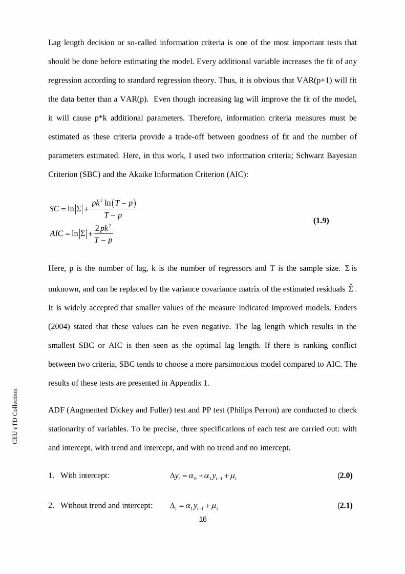
Lag length decision or so-called information criteria is one of the most important tests that

should be done before estimating the model. Every additional variable increases the fit of any

regression according to standard regression theory. Thus, it is obvious that VAR(p+1) will fit

the data better than a VAR(p). Even though increasing lag will improve the fit of the model,

it will cause p*k additional parameters. Therefore, information criteria measures must be

estimated as these criteria provide a trade-off between goodness of fit and the number of

parameters estimated. Here, in this work, I used two information criteria; Schwarz Bayesian

Criterion (SBC) and the Akaike Information Criterion (AIC):

2

2

lnln

2ln

pk T pSC

T ppkAIC

T p

(1.9)

Here, p is the number of lag, k is the number of regressors and T is the sample size. is

unknown, and can be replaced by the variance covariance matrix of the estimated residuals ˆ .

It is widely accepted that smaller values of the measure indicated improved models. Enders

(2004) stated that these values can be even negative. The lag length which results in the

smallest SBC or AIC is then seen as the optimal lag length. If there is ranking conflict

between two criteria, SBC tends to choose a more parsimonious model compared to AIC. The

results of these tests are presented in Appendix 1.

ADF (Augmented Dickey and Fuller) test and PP test (Philips Perron) are conducted to check

stationarity of variables. To be precise, three specifications of each test are carried out: with

and intercept, with trend and intercept, and with no trend and no intercept.

1. With intercept: 0 1 1t t ty y (2.0)

2. Without trend and intercept: 1 1t t ty (2.1)

CE

UeT

DC

olle

ctio

n

17

Francesco Guidi et al (2009) test the following hypothesis:

0

1

: =0 (Unit Root)H : 0H

(2.2)

Conventional t-ratio for is used to evaluate the hypothesis:

ˆˆ( )

tse

(2.3)

Here, ˆ is the estimate of . However, Dickey and Fuller (1979) have shown that under the

null hypothesis of a unit root, we can not use the conventional t-distribution. In such situation

the following can be applied to make decision:

critical value reject null hypothesis (unit root exists)

critical value null hypothesis (unit root does not exist)

t ADF not

t ADF reject

Moreover, I have used a Philips-Perron (PP) Test to check stationarity of variables. The null

hypothesis that the variable has a unit root is rejected for all specifications of oil price shocks

except linear oil price shocks by both tests at the conventional levels. Linear oil price shock

has unit root. Log levels of the real effective exchange rate, real government expenditures,

real export, real GDP and log of seasonally adjusted inflation are found to be unit root

processes. Both tests show that these variables are I(1) processes. This simply means that in

the case of the variables that have unit roots both tests reveals that their log differences are

stationary.

CE

UeT

DC

olle

ctio

n

18

5 Methodology

5.1 Foundations for VAR Methodology

Whenever, we have several time series, we have to take into account the interdependence

between them. There are number of ways to work with multiple time series, one can estimate

a simultaneous equations model with lags on all variables. However, doing this, we need to

first, classify variables into two categories; endogenous and exogenous. Second, to achieve

identification we have to impose some constraints on the parameters.4 These steps involve

difficult justification. As an alternative Sims (1980) suggests the vector autoregression (VAR)

approach.

Thus, I will use an unrestricted VAR model to investigate the response of macroeconomic

variables to positive and negative innovations in oil prices. The VAR model provides a

multivariate approach where changes in its own lags and to changes in other variables and the

lags of those variables. In fact, VAR model regresses each variable from a set of variables on

its own lagged values together with the lagged values of the other variables. Basically, the

VAR framework is conducted to avoid endogeneity concerns. The VAR treats all variables as

endogenous and does not impose a priori restrictions on structural relationships. Given that

VAR expresses the dependent variables in terms of predetermined lagged variables, it is a

reduced form model. Macroeconomic study of oil price shocks can be studied by employing

alternative approach. Particularly, structural vector autoregressive models (SVAR) better suits

to oil price shocks analysis. SVAR models identify the variance decomposition and impulse

response functions by imposing a priori restrictions on the covariance matrix of the structural

4 Maddala et al (2001)

CE

UeT

DC

olle

ctio

n

19

errors. However, validity of priori restrictions is quite disputable, thus making SVAR models

less applicable.

Furthermore, before estimating unrestricted VAR model, I need to decide whether I have to

use a VAR model in levels or in first differences. Not all the variables in my model follow a

I(0) process. This is quite intuitive as the most time-series variables exhibits non-stationarity

patterns. Hamilton (1994) suggests that one option is to ignore the non-stationarity altogether

and simply estimate the VAR in levels. The other alternative is consistently to difference any

apparently non-stationary variables before estimating the VAR. Other than that it should also

be discussed whether an unrestricted VAR should be used where the variables in the VAR are

cointegrated. There is number of authors who support the use of a vector error correction

model (VECM), or cointegrating VAR in such a situation. Even though 5 of six variables are

I(1) process, I decided not to estimate Vector Error Correction models. It has been argued that

in the short term, unrestricted VAR perform better than a cointegrated VAR or VECM. The

reason for such a conclusion is sample period. In my model, I use short sample, therefore

employing VECM instead of unrestricted VAR may cause to reject the null of no

cointegration in small samples. The advantages of unrestricted VAR over VECM can be

demonstrated by analyzing impulse response functions in cointegrated systems. 5 Naka and

Tufte (1997) estimated system of cointegrated variables as a VAR in levels and as a VECM

model. VECM estimates perform poorly relative to those from a VAR. Naka and Tufte

(1997) through Monte Carlo simulations also concluded that the loss of efficiency in the VAR

estimations of cointegrating variables was not critical for the commonly used short horizon.

Moreover, Engle and Yoo (1987), Clements and Hendry (1995) and Hoffman and Rasche

5 Naka and Tufte (1997)

CE

UeT

DC

olle

ctio

n

20

(1996) conclude that when imposed restrictions are true, an unrestricted VAR produces more

superior forecast variance than a restricted VEC model on short horizons.

Finally, considering the existence of equilibrium relationships among non-stationary variables

in the system and the mentioned discussions about advantages and shortcomings of different

VAR frameworks, I decide to employ an unrestricted VAR system.

5.2 Unrestricted VAR

Our unrestricted vector autoregressive model in reduced form of order p is presented in

following equation:

t i t i ty c A y (2.4)

Where 1 6.......c c c is the 6 1 intercept vector of the VAR, iA is the thi 6 6 matrix of

autoregressive coefficients for i=1, 2….p, and 1, 6,,.......,t t t is the 6 1 generalization

of a white noise process.

As described in data section, we use six endogenous macroeconomic variables in our system:

roilp, rgovexp, rgdp, inf, reer, and rexp (all in logarithms). The form of unrestricted VAR

system in this work is given by6:

6 Similar methodology was used by Mohammad Reza Farzanegan et al (2007)

CE

UeT

DC

olle

ctio

n

21

exp

inf

exp

roilprgovrgdp

reerr

=

1

2

3

4

5

6

cccccc

+ A(I)

1

1

1

1

1

1

exp

inf

exp

t

t

t

t

t

t

roilprgovrgdp

reerr

+

1

2

3

4

5

6

t

t

t

t

t

t

(2.5)

Where A(l) is the lag polynomial operators, error vectors are mean zero.

( ) 0iE for all t, ( )t sE if s=t and ( ) 0t sE if s t . Here, is the variance-

covariance matrix. Errors are not serially correlated but might be contemporaneously

correlated. Thus, is assumed to have non-zero off diagonal elements. As pointed out by

Hamilton (1994), the VAR system can be transformed into its vector ( )MA representation.

This transformation mainly serves to analyze impacts of real oil price shocks:

1 1 2 2 ....t t t ty (2.6)

Above equation can be re-written as:

0t i t i

iy (2.7)

With 0 being identity matrix and is the mean of the process:

1

1

p

p ii

I A c (2.8)

The reason of applying moving average representation is generate the forecast error variance

decomposition (VDC) and the impulse response functions (IRF).

CE

UeT

DC

olle

ctio

n

22

In this study, the innovations of current and past one-step ahead forecasts errors are

orthogonalised using Cholesky decomposition so that the resulting covariance matrix is

diagonal. According to this methodology the first variable in a pre-specified ordering has an

immediate impact on all variables in the system besides first variables and so on. Thus, pre-

specified ordering is vital and can alter the dynamics of a VAR system. We can describe the

vector of exogenous variables in the following way:

tan , Z1, Z2, Z3, Z4, Z5ty cons t (2.9)

Here, Z1-Z5 represents all other important exogeneous variables during the period of 1998-

2009.

Another important issue in the VAR estimation is the lag order selection. Akaike Information

Criteria (AIC), Schwarz Information Criterion (SC), and Hannan-Quinn Information Criterion

are the most applicable criteria used in lag order selection procedure. Usually, four lags can be

included in case of quarterly data or twelwe lags in case of monthly data. Similarly, we can

choose the lag order to be one if we have yearly data. In this work traditional criteria often

suggest different number of lags; inverse root test indicates stability of all lags tried, but

autocorrelation LM test points out the presence of the serial correlation in the errors when 12th

lag included. Likelihood Ratio (LR) shows that 11th lag is significant and should be included,

however, other criteria such as AIC, and FPE indicates 2nd lag to be included. In the meantime

SC and HQ point out 1st lag to be included. These different results lead to the conclusion that

VAR does not adequately represent the data generating process. Thus, the approach used here

is to choose the minimum number of lags confirming the stability and no serial correlation

conditions are satisfied.

CE

UeT

DC

olle

ctio

n

23

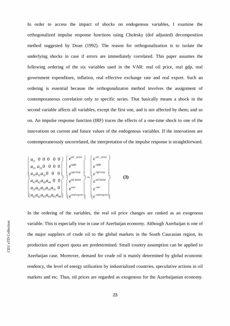
In order to access the impact of shocks on endogenous variables, I examine the

orthogonalized impulse response functions using Cholesky (dof adjusted) decomposition

method suggested by Doan (1992). The reason for orthogonalization is to isolate the

underlying shocks in case if errors are immediately correlated. This paper assumes the

following ordering of the six variables used in the VAR: real oil price, real gdp, real

government expenditure, inflation, real effective exchange rate and real export. Such an

ordering is essential because the orthogonalizaton method involves the assignment of

contemporaneous correlation only to specific series. That basically means a shock in the

second variable affects all variables, except the first one, and is not affected by them; and so

on. An impulse response function (IRF) traces the effects of a one-time shock to one of the

innovations on current and future values of the endogenous variables. If the innovations are

contemporaneously uncorrelated, the interpretation of the impulse response is straightforward.

_11

21 22exp

31 32 33

inf41 42 43 44

51 52 53 54 55

exp61 62 63 64 65 66

0 0 0 0 0 0 0 0 0

0 0 0 0 0

0

oil price

rgdp

rgov

lation

reer

real ort

eaea a

a a a ea a a a ea a a a a ea a a a a a e

_

exp

inf

exp

oil price

rgdp

rgov

lation

reer

real ort

(3)

In the ordering of the variables, the real oil price changes are ranked as an exogenous

variable. This is especially true in case of Azerbaijan economy. Although Azerbaijan is one of

the major suppliers of crude oil to the global markets in the South Caucasian region, its

production and export quota are predetermined. Small country assumption can be applied to

Azerbaijan case. Moreover, demand for crude oil is mainly determined by global economic

tendency, the level of energy utilization by industrialized countries, speculative actions in oil

markets and etc. Thus, oil prices are regarded as exogenous for the Azerbaijanian economy.

CE

UeT

DC

olle

ctio

n

24

Significant shocks in oil markets affect contamperaneously the other key macro economic

variables in the system.

I choose the real government expenditures as a second variable in this ordering. Government

expenditures include recurrent and capital consumptions. Expenditures on government

employees and subsidies can be classified as recurrent expenditures, while capital

expenditures aim to increase rather than keep stable the physical and material assets of an

economy. During 2005-2007, when the first oil boom started, the government of Azerbaijan

decided on extraordinarily large expenditure increases aimed at improving infrastructure and

raising incomes. Such an exceptional magnitude of government spending shows the role of

government. Actually, the role of the government has also been on the increase since 1995

which automatically reflects in the expansion in total government spending. This is due to the

fact that the government is the main recipient of oil rents and attempts to distribute them

through increases in investments on infrastructure and salaries which blow up government

spending. Total government expenditure increased by a cumulative 160 percent in nominal

terms from 2005 to 2007 or from 41 percent of non-oil GDP to 74 percent. (Junko Koeda and

Vitali Kramarenko, 2008). This large increase in expenditures raised the question whether the

current level of expenditure is appropriate and sustainable in long term prospective.

The third variable included in this ordering is real GDP. It is worth to note that industrial

production is alse affected instantly by the level of government demand. The positive

development in oil prices which automatically results in increases of government expenditures

and income per capita. This increase in government expenditure and income pushes the

effective demand upward. Moreover, inefficiencies in overall economy, lack of domestic

supply, time lags in response to increased demand may lead the consumer prices upward

resulting in inflation.

CE

UeT

DC

olle

ctio

n

25

Eventually, increase in inflation results in real effective exchange rate appreciation. The

relative prices of non-tradable goods to tradable goods are measured by the real effective

exchange rate which is defined as a weighted real exchange rate index. Whenever domestic

prices increase the relative prices of non-tradable goods will increase, while prices abroad

remain unchanged. This would result in loss of competitiveness of an economy. In this study,

I assume that a shock in real effective exchange rate contemporaneously affects real export in

Azerbaijan.

Runkle (1987) suggests reporting impulse response functions with standard error bands. As

an indication of significance, I have estimated 95% confidence intervals for the IRF’s. These

confidence bands are obtained from 1000 draw Monte Carlo simulations. The middle lines in

the figures represent the impulse response function while the bands stand for the confidence

intervals. The null hypothesis that there is no effect of oil price shocks on other

macroeconomic variables cannot be rejected if and only if the horizontal line falls into the

confidence interval.

Thus, the impulse response functions illustrate the qualitative response of the variables in the

system of shocks to real oil prices. However, we need a variance decomposition to indicate

the relative importance of these shocks. It tells us how many unforeseen variations of the

variables in the model are explained by different shocks. To get this, I considered the n-step

ahead forecast of a variable based on information at time t. Here, I applied four sets of

variance decompositions for symmetric, asymmetric (positive and negative formations of oil

prices), and NOPI (net oil price increase) formations of oil prices.

The computation of variance decomposition also requires identification. The identification is

achieved by imposing the same structure as in the case of impulse responses. Again, the

standard errors are also calculated via Monte Carlo simulations with 1000 repetitions

CE

UeT

DC

olle

ctio

n

26

6 Empirical Results

In this section, I will discuss empirical results and analysis of the VAR model. Particularly, I

will analyze effects of oil price shocks on the macroeconomy of Azerbaijan by using three

analytical tools: Granger causality, impulse response functions and variance decomposition.

Additionally, the results will be compared to those of other papers.

It is worth to note that when lower triangular Cholesky decomposition is employed, changing

orderings of variables for impulse responses and variance decompositions can give different

results. For robustness test we make use of an alternative ordering which is based on VAR

Granger Causality: oil price shock, inflation, GDP growth, real export, real government

expenditure and real effective exchange rate.7 Even though I presented results of each

specification of oil price shocks, the conclusion and policy implications will be mainly based

on the linear oil price shock model. Based on the principles stated on the methodology part for

each model I include two lags.

The results for Granger causality test for the variables are presented in Appendix II. It has

been found that positive oil price shocks do not Granger cause macroeconomic variables. The

Granger causality test also shows that there exists causality between oil price changes and

government expenditure as well as between oil price changes and inflation in the case of

negative oil price shocks. For the case of NOPI specification I have found that NOPI

specification of oil price shocks does not Granger cause any of the macroeconomic variables.

Tests for symmetric oil price shocks model indicates that symmetric oil price shocks Granger

cause significantly inflation (at 1% significant level). This finding more likely implies that

monetary stability in oil exporting transition economy is more sensitive to past oil price

7 Jimenez-Rodriguez (2007) replaced real effective exchange rate at the end, explaining this by the fact that realexchange rate as an asset price should be contemporaneously affected by all macroeconomic variables.

CE

UeT

DC

olle

ctio

n

27

movements in both direction and in all specifications of oil price shocks except for positive oil

price shocks. Another findings for symmetric oil price shocks is that symmetric oil price

shocks can significantly help predicting real effectice exchange rate (at 5% significant level).

Surprizing result is that almost all specifications of oil price shocks do not Granger cause

GDP.

Based on the results of the tests, I can confirm that past movements of negative oil price

changes, and symmetric oil price changes forecasts current movements in inflation. For a

prediction of real effective exchange rate only symmetric oil price changes can be used and

changes in real export can be best explained using again symmetric oil price shock model.

6.1 Impulse Response functions: Linear Specification

Under this section I examine the effects of oil prices macroeconomic variables using

orthogonalised impulse response functions for the linear, net and non-linear specifications of

the model. Figure 1 shows IRFs base on one standard deviation shock to linear specification

of oil price shock. For real GDP growth and real government expenditures the null hypothesis

of no effect of oil price changes on GDP cannot be rejected at the five percent level. Based on

Monte Carlo confidence bands I can judge that response of GDP is insignificant. The response

of inflation to innovations in oil prices is significantly positive. This response is completely

significant within a year. Response of inflation to oil price shock gradually rises from initial

level to 0.004 percent during the first three months following the shock. In the first quarter the

increase in inflation above its initial level reaches 0.0045 percent in linear specification. After

half year the impact gets to 0.005 percent and stays at constant 0.005 percent exactly one year

after the shock. This suggests that the impact of oil price shock on inflation in Azerbaijan is

relatively persistent and shows the long-run inflationary effects of oil price increases on the

CE

UeT

DC

olle

ctio

n

28

Azerbaijani economy. Such a response can be defined as a “spending effect”.8 Spending effect

can also be explained by AD-AS model. Azerbaijan is an oil exporting country and oil price

increases result in speedy increase of government spending. Thus, spending effect occurs

because higher oil prices lead to higher wages in the oil related sectors. Increase in income

distribution takes place, thus, increasing power of purchase and demand in the economy.

While oil prices are exogenous and only international markets may determine price of oil, the

price of non-tradable sections like services is determined within the national market. Push

demand inflation in non-tradable sections emerges due to the fact that some fraction of

increased demand is shifted to this sector. Here, we explicitly assume that there is no trade-off

between tradeable and non-tradeable sectors. Hence, we do not have to take account for

transfer of workers from oil sector to non-oil sector.

Another important channel is the effect of oil price shock on the level of real exchange rate.

However, the response of real effective exchange rate to linear oil price shocks is only

significant in the first month following the shock. As shock happens real effective exchange

rate falls by 0.004 percent below its initial level, but after that I observe a positive response

and increasing trend of this variable. As a net exporter of oil, Azerbaijan’s real effective

exchange rate appreciates starting from the first quarter. This may lead to higher inflow of

foreign exchange into the economy which was actually the case in the early 2000s. Foreign

direct investments to the economy are a positive sign, but, it still has serious drawbacks and

implications on real economic activities due to the reliance of the economy on foreign inputs.

Starting from the first quarter real effective exchange rate appreciates in increasing temp, thus

8 Corden (1984) explains both short run and long run inflationary effects of oil price increases within the“resource movement” and “spending effect” framework. According to Corden resource movement takes placewhen the production factors such as labor can easily move between oil and non-oil sectors. In such a way, oilprice increases lead to absorbtion of labor from other sections of economy. Labor qualification between oiland non-oil industries are not similar and oil industries require high capital intensity, therefore, resourcemovement can not be related to Azerbaijan case.

CE

UeT

DC

olle

ctio

n

29

reaching 0.009 percent at the end of the year following the shock. This could be a sign of the

“Dutch Disease”in the long run after oil price shock. “Dutch Disease” can lead to reduction in

the competitiveness of the tradable sector of Azerbaijani economy. However, the response of

this variable is not significant.

The response of real government expenditure to one standard shock to linear oil price changes

is not significantly different from zero. Thus, the null hypothesis of no effect of oil price

changes on real government expenditure can not be rejected. This is quite challenging result,

as it is totally contradicts with my initial assumption. However, this can be explained by the

fact that Azerbaijan government has established State Oil Fund of Azerbaijan (SOFAZ) in

1999 in order to save large part of the windfall oil revenues in an oil fund.9 The main goals of

Fund are to achieve macroeconomic stability, decrease dependence on oil revenues and

stimulate the development of non-oil sector. Fund uses only part of oil revenue to finance the

capital expenditures, major national scale projects to support socio-economic growth. Fund

accumulates and preserves oil revenues for future generations, therefore, it can be concluded

that Fund has an effective mechanism for oil wealth management. As we have seen above,

real effective exchange rate has a positive response and increasing trend, however is not

significant. This is against to our beliefs about “Dutch Disease”. According to “Dutch

Disease” we expect significant appreciation of real effective exchange rate in the case of

positive oil price shocks. This phenomenon can be explained by the role of Fund stated above.

Hence, the establishment of oil stabilization fund and controlling government expenditures

helped government to successfully save unexpected oil revenue increases for next

generations. By controlling government expenditures Fund could successfully tackle with

possible appreciation in effective exchange rate.

9 http://www.oilfund.az/az

CE

UeT

DC

olle

ctio

n

30

Finally, based on Monte Carlo confidence bands I can judge that response of the real export to

one standard shock to linear oil price changes is significant. However, I have to include that

this response becomes significant only after third month following the shock. In the third

month at the time when response becomes significant, real export reaches its maximum; 0.91

percent. In the long run real export experiences a decrease to its initial level, though this

decrease still remains significant in the long run.

6.2 Impulse Response Functions: Asymmetric and Net Specification

The impulse responses for the non-linear or asymmetric and net oil specifications are

presented in Figures 2-4. Within NOPI specification none of the variables has signicant

responses to net oil price increases. Based on Monte Carlo confidence bands it can be

concluded that the response of the inflation, real government expenditure, real effective

exchange rate, real export, real GDP growth to one standard shock net oil price increases is

not significant and the null hypothesis of no effect of oil price changes on macroeconomic

variables can not be rejected at the 5 percent level.

Under asymmetric shocks inflation again is significant, and has the similar pattern to those of

under symmetric. Thus, in the third month following the shock inflation reaches its maximum

0.002 percent. Starting from the first quarter this increase weakens and becomes insignificant

and dies out completely within the year after the shock. The response of real effective

exchange rate to is worth to describe in detail. In Appendix III, Figure 2, I demonstrate the

responses of variables to negative changes in real oil prices. The most interesting pattern here

is the response of real effective exchange rate. Even though it is insignificant during the

whole period, the response of the real effective exchange rate to a decreasing real oil prices is

negative. It reaches its minimum in the first month as soon as shock happens. Decrease in real

CE

UeT

DC

olle

ctio

n

31

effective exchange rate can be explained by the fact that government had approved export-

friendly policies to relieve the impact of declining oil prices. In addition, government

stimulates non-oil sections to improve their competitiveness. Thus, reduction in real effective

exchange rate leads to improvement in competitiveness in non-oil sections. The responses of

other variables to negative oil price shock are not significant.

6.3 Variance Decomposition Analysis

In this section I will attempt to give the forecast error variance decomposition analysis for all

four models: linear, non-linear or asymmetric and net oil price specifications. Variance

decomposition tells us how many unforeseen changes or variations of the variables are

explained by different shocks.

Tables 1-5 demonstrate the variance decomposition of the VAR model. As I have expected

contributions of symmetric oil price shocks and the other specifications of oil price increases

particularly both non-linear models and net oil specifications to GDP growth variation are not

statistically significant during all ten months given any significance level10. For inflation,

negative oil price shocks account for approximately 10 percent of its variation in the third

period, remains significant to the end of the tenth period and increases to 14 percent. In order

words, in the tenth period for inflation negative oil price shocks account for 14 percent of its

variation. Contributions of symmetric oil price shocks to inflation variation are statistically

significant at 10 percent only starting from third period and accounts for 9.93 percent of its

variation increasing to 23 percent in 10 periods after shock. This high inflationary pressure

results from increased spending which comes from solely oil revenues.

10 Dotsey and Reid (1992) revealed that 5-6 % of variations in GNP can be explained by oil prices, and accordingto Brown and Yucel (1992) variations in output are poorly explained by oil prices.

CE

UeT

DC

olle

ctio

n

32

For real effective exchange rate the contribution of none of the models are statistically

significant during all ten months.

The other important aspect of the symmetric oil shock can be seen in the effects on real export

fluctuation. Linear or symmetric oil price shock explains for about 4.4 percent of fluctuations

in the real export in the third month after shock, increasing to about 11.6 in the 10th month

after the shock.

Considering the results of all specifications, I claim that the contribution of oil price decreases

and symmetric oil price shock is quite large in the variation of inflation in Azerbaijan. Its

average shares are 9 percent. Seemingly, in all cases, the oil contribution to variations of

inflation and real export is significant mostly from the third month.

6.4 Comparative Analysis of Results

In this section I will compare the empirical results of this thesis with the results of two other

papers. Particularly I will make comparative analysis of results of Aliyu et al (2009) on

Nigeria (oil exporter country), and Mohammad Reza Farzanegan et al (2007) on Iranian

economy.

Mohammad Reza Farzanegan et al (2007) shows that due to the high dependence on oil

revenues, oil price changes impacts Iranian economy. Historically empirical findings indicate

that oil price increases have a significant positive effect on industrial output for oil importing

countries. Farzanegan et al (2007) reveals that there is no significant impact of oil price

changes on real government expenditures. Farzanegan also indicates that the response of real

imports and the real effective exchange rate to asymmetric oil price shocks are significant. In

addition Farzanegan and Markwardt state that the response of inflation to any kind of oil price

CE

UeT

DC

olle

ctio

n

33

shocks is significant and positive. In my thesis I found that positive oil price shocks do not

Granger cause macroeconomic variables. However, the Granger causality tests of my work

exhibits that there is causality between oil price changes and government expenditure as well

as between oil price changes and inflation in the case of negative oil price shocks. For the

case of NOPI specification I have found that NOPI specification of oil price shocks Granger

causes government expenditures and inflation. Tests for symmetric oil price shocks model

indicates that symmetric oil price shocks Granger cause significantly inflation (at 1%

significant level). In addition the response of inflation to innovations in oil prices is

significantly positive. This response is completely significant within a year. Thus, my result is

in line with Farzanegan et al (2009) that in oil exporting countries oil price shocks positively

affect inflation. I concluded that impact of oil price shock on inflation in Azerbaijan is

relatively persistent and shows the long-run inflationary effects of oil price increases on the

Azerbaijani economy. I explained this phenomenon based on the studies of Corden (1984).

Corden explains both short run and long run inflationary effects of oil price increases within

the “resource movement” and “spending effect” framework. Farzanegan uses the same

“spending effect” to analyze the consequences of oil price shocks. Farzanegan and Markwardt

also failed to identify a significant impact of oil price fluctuation on real government

expenditures. In my thesis I have got similar result. This result is quite challenging as I

expected to see the impact of positive oil price shock on real government expenditures.

During 2005-2007, when the first oil boom started, the government of Azerbaijan decided on

extraordinarily large expenditure increases aimed at improving infrastructure and raising

incomes. Such an exceptional magnitude of government spending shows the role of

government. Thus, before running tests I hoped to get positive changes in real government

expenditures. However, impulse response functions analysis indicates that the null hypothesis

of no effect of oil price changes on real government expenditure can not be rejected.

CE

UeT

DC

olle

ctio

n

34

Farzanegan et al (2007) got the same result. They explained this with the increased role of

government policy of saving a large part of the windfall oil revenues in an oil stabilization

fund starting from 2000. Similar patterns can be observed in my thesis as well. Azerbaijan

government has also established State Oil Fund of Azerbaijan (SOFAZ) in 1999 in order to

save large part of the windfall oil revenues in an oil fund. SOFAZ uses them to finance

national scale projects and pay back external debts. SOFAZ avoids spendings for current

expenditures thus creating effective mechanism for management of oil revenues. Finally,

Farzanegan et al (2007) reveals that the response of the real effective exchange rate to

asymmetric oil price shocks are significant. In a contrary, my thesis work revealed that the

responses of real effective exchange rate based on Monte Carlo confidence bands are not

significant under neither linear nor non-linear oil price shocks. However, I presented the

results of responses of real effective exchange rate to show that these results are contrary to

priori expectations of encountering “Dutch Disease”. The establishment of SOFAZ in

Azerbaijan controls government expenditure and partly absorbs the unexpected oil revenue

increases and possible appreciation in effective exchange rate.

Aliyu (2009) employed Granger causality tests and multivariate VAR analysis using both

linear and non-linear specifications. Aliyu (2009) found evidence of both linear and non-

linear impact of oil price shocks on real GDP growth. Aliyu (2009) states that asymmetric oil

price increases in the non-linear models have larger positive impact on real GDP growth than

asymmetric oil price decreases adversely affects real GDP. In my thesis, Granger causality

tests and impulse response functions analyzes leads to the conclusion that in both short run

and long run the null hypothesis of no effect of oil price changes on GDP cannot be rejected

at the five percent level. Based on Monte Carlo confidence bands I can judge that response of

GDP is insignificant.

CE

UeT

DC

olle

ctio

n

35

7 Conclusions and Policy Implications

This thesis concludes that oil price shocks really matter for Azerbaijan. Therefore, policy

makers of Azerbaijan should account for oil price fluctuation while making decisions on

monetary and fiscal policies.

Linear oil price shock Granger causes inflation, have a positive effect on it and play a

significant role in its variation. The impact of oil price shock on inflation in Azerbaijan is

relatively persistent and shows the long-run inflationary effects of oil price increases on the

Azerbaijani economy. I defined this result as a “spending effect”. As Corden (1984) and

Farzanegan et al (2007) explained, “spending effect” occurs due to the fact that higher oil

prices guide to higher labor compensation or incomes in the oil related sectors. This increase

in wages raises the aggregate purchasing power and aggregate demand in the economy.

Tradeable sections include oil and manufacturing sectors and the price of these sections pre-

determined in the international markets. However, the price of non-tradeable sections which

include services industry is endogenous and determined within the domestic market. Part of

increased aggregate demand shifts to non-tradeable section, thus resulting in push-demand

inflation in this section. It is worth to note that here I assumed the immobility between

tradeable and non-tradeable sectors. If that was not the case, then we would encounter transfer

of workers from oil and manufacturing section to booming service section. So, in the case of

immobility between tradeable and non-tradeable sectors the supply of services remains

constant, even though the price of services increases.

Unexpectedly the response of real government expenditure to one standard shock to linear oil

price changes is not significantly different from zero. Thus, the null hypothesis of no effect of

oil price changes on real government expenditure can not be rejected. During 2005-2007,

when the first oil boom started, the government of Azerbaijan decided on extraordinarily large

CE

UeT

DC

olle

ctio

n

36

expenditure increases aimed at improving infrastructure and raising incomes. However, Fund

uses only part of oil revenue to finance the capital expenditures, major national scale projects

to support socio-economic growth. Fund accumulates and preserves oil revenues for future

generations, therefore, it can be concluded that Fund has an effective mechanism for oil

wealth management. This can explain why response of real government expenditure to one

standard shock to linear oil price changes is not significantly different from zero.

The fact that the responses of real effective exchange rate to oil price changes are not

significant can be explained due to the fact that Central Bank of Azerbaijan employs fixed

exchange rate regime. Real effective exchange rate has a positive response and increasing

trend in case of linear oil price shock, however, the response of real effective exchange rate to

linear oil price change is still not significant. The response of real exchange rate remain

insignificant in the case of positive oil price shock and even more we observe initial decrease

in real effective exchange rate. Starting from the third month, responses to innovations in

positive oil prices begin to increase, and then gradually completely dies out. This is against to

our beliefs about “Dutch Disease”. According to “Dutch Disease” we expect significant

appreciation of real effective exchange rate in the case of positive oil price shocks. The role of

State Oil Fund of Azerbaijan is magnificient here. The establishment of oil stabilization fund

and controlling government expenditures helped government to successfully save unexpected

oil revenue increases for next generations. By controlling government expenditures Fund

could successfully tackle with possible appreciation in effective exchange rate.

The response of industry output in all specifications is not significant. Seemingly, additional

researches have to be conducted in order to reveal this phenomenon. Studies done before

Hamilton (2003) and Jimenez-Rodriguez and Sanchez (2004) find that for developed

economies impact of positive oil price shocks on real GDP growth is much larger than impact

CE

UeT

DC

olle

ctio

n

37

of negative shocks. Thus, increases in oil prices leads to significant reduction in domestic

output, while decreases in oil prices cause only marginal effect in industrial economies. In my

thesis work, I revealed that Azerbaijan as a developing country and net oil exporter exhibits

that both positive and negative oil price changes and linear oil price fluctuations does not have

a significant affect on the gross output. This result is quite challenging and requires more

detailed research to find out what are the side effects.

The overall performance of the Azerbaijani monetary and fiscal authorities is adequate. The

possible policy implication for the Azerbaijani government is to increase transparency within

the State Oil Fund of Azerbaijan and to decrease the influence of the government to Fund to

provide efficient and sound mechanism of Fund. Oil revenues can lead to the wealth of the

nation and at the same time to threaten the future generations in Azerbaijan. Nonetheless, oil

is the nation’s treasure, and therefore, the best practises for windfall oil funds management

must be taken into account by the policymakers of the Azerbaijan.

CE

UeT

DC

olle

ctio

n

38

8 ReferencesAnashasy, E.A. 2005. “Evidence on the role of oil prices in Venezuela’s economicperformance: 1950-2001”, Working Paper, University of Washington

Atmadja, A.S. 2005. “The Granger causality tests for the five ASEAN countries’ stockmarkets and macroeconomic variables during and post the 1997 Asian financial crisis”, JurnalManajemen and Kewirausahaan, Vol. 7

Bernanke, B.S., Gertler, M and Watson M. 1997. “Systematic monetary policy and the effectsof oil price shocks”. Brooking Papers on Economic Activity, No 1

Blanchard, O.J and J.Gali, 2007. “The Macroeconomic effects of Oil Price Shocks: Why arethe 2000s different from the 1970s?.” MIT department of Economics Working Paper No. 07-21

Central Bank of Azerbaijan Database

Corden, M.W. 1984. “Booming Sector and Dutch disease Economics” Survey andConsolidation, Oxford economics papers 36, 359-380

Clements, M.P. and Hendry, D.F. 1995. “Forecasting in Cointegrated Systems”, Journal ofApplied Econometrics, Vol. 10

Cunado, J. and Garcia F.P. 2005. “Oil prices, Eonomic activity and Inflation: Evidence forsome Asian countries”. The quarterly Review of Economics and Finance, Vol. 45

Dahl, C.A., and M. Yucel. 1991. “Testing Alternative Hypothesis of Oil Producer Behavior”,Energy Journal 12(4): 117-138

Darby, M.R. 1982. “The Price of Oil and World Inflation and Recessions”, AmericanEconomic Review, Vol 72.

Dickey, D.A. and Fuller W.A. 1979. “Distribution of the Estimators for Autoregressive timeseries with a Unit Root”, Journal of the American Statistical Association, Vol. 74

Farzanegan M. R and Markwardt G. 2007. “The Effects of Oil price Shocks on the IranianEconomy”, Faculty of Business, Dresden University of Technology, D-01062, Dreden,Germany.

Gordon, Robert J. 1984. “Supply Shocks and Monetary Policy Revisited”. AmericanEconomic Review. Vol. 74(2) 38-43.

Granger, C.W.J 1969. “Investigating Causal Relations by Econometric Models and Cross-Spectral Methods, Econometrica Vol.37, 424-438.

Griffin, J. M. 1985. "OPEC Behavior: A Test of Alternative Hypotheses," AmericanEconomic Review Vol. 75, pp. 954-963.

Gounder, R and Bartleet M. 2007. “Oil Price Shocks and Economic Growth: Evidence forNew Zealand, 1989-2006” Paper Presented at New Zealand Association of Economist AnnualConference, Christchurch, 27th to 29th June, 2007.

Hamilton, James D. 2003. “What is an oil shocks?” Journal of Econometrics, Vol. 113

CE

UeT

DC

olle

ctio

n

39

Hamilton, James D. 1983. “Oil and the Macroeconomy since World War II”, Journal ofPolitical Economy, Vol. 91

Hoffman, D.L. and Rasche, R.H. 1996. “Assessin forecast performance in a cointegratedSystem”, Journal of Applied Econometrics, Vol. 11

Hooker, M.A. 1996. “What Happened to the Oil Price Macroeconomy Relationship?” Journalof Monetary Economics Vol. 38, 195-213.

Jimenez-Rodriguez, R. and Sanchez, R.H. 2005. “Oil price shocks and real GDP growth:empirical evidence for some OECD countries”, Applied Economics, Vol. 37

Jimenez-Rodriguez, R. 2007. “The industrial impact of oil price shocks: Evidence from theindustries of six OECD countries.” Working paper of the Bank of Spain No. 0731

Johansen, S. 1991. “Estimation and Hypothesis Testing of Cointegration Vectors in GaussianVector Autoregressive Models” Econometrica Vol. 59, 1551-1580.

Jones, R. and P.B. Kenen (eds.) 1985. Handbook of International Economics: Vol. 2

Joyce, J.P. and L. Kamas. 1997. ‘The Relative Importance of foreign and domestic shocks toOutput and prices in Mexico and Colombia’, Weitwirtschaftliche Archiv, Vol. 133(3), 458-477

Lee, K., Ni, S, and Ratti, R. 1995. “Oil Shocks and the Macroeconomy: The Role of the PriceVariability.” Energy Journal, Vol. 16

Lutkepohl, H. 2004. “Vector Autoregressive and Vector Error Correction Models” Appliedtime series econometrics, ed. By Lutkepohl, H. and Kratzig, M. New York: CambridgeUniversity Press

Mork (1994): “Business Cycles and the Oil Market”, The Energy Journal, 15 (Special Issue),The changing World petroleum Market, 39-67.

CE

UeT

DC

olle

ctio

n

40

9 Appendix I

9.1 Results of Unit Root Tests Oil Price ShocksADF Test (p values in cells)

H0: a variable has a unit rootVariables

None constant

level 1st dif level 1st diff

Oil price shock 0.8280 0.0000 0.6674 0.0000

Oil price shock+ 0.0006 0.0000 0.0000 0.0000

Oil price shock- 0.0000 0.0000 0.0000 0.0000

NOPI 0.0002 0.0000 0.0004 0.0000

PP Test (p values in cells)

H0: a variable has a unit rootVariables

None constant

level 1st dif level 1st diff

Oil price shock 0.7858 0.0000 0.4932 0.0000

Oil price shock+ 0.0000 0.0001 0.0000 0.0001

Oil price shock- 0.0000 0.0001 0.0000 0.0001

NOPI 0.0002 0.0000 0.0000 0.0001

CE

UeT

DC

olle

ctio

n

41

9.2 Macroeconomic variables of Azerbaijan

ADF Test (p values in cells)

H0: a variable has a unit rootVariables

None constant

level 1st dif level 1st diff

Inflation 0.9999 0.0000 0.9998 0.0000

Real GDP 0.9925 0.0000 0.9119 0.0000

Real Government Expenditure 0.9905 0.0000 0.5200 0.0000

Real Effective Exchange Rate 0.9047 0.0000 0.8937 0.0000

Real Export 0.8762 0.0000 0.6520 0.0000

PP Test (p values in cells)

H0: a variable has a unit rootVariables

None constant

level 1st dif level 1st diff

Inflation 1.0000 0.0000 0.9984 0.0000

Real GDP 0.9952 0.0000 0.8987 0.0000

Real Government Expenditure 0.9273 0.0000 0.1559 0.0001

Real Effective Exchange Rate 0.8563 0.0000 0.7829 0.0000

Real Export 0.8186 0.0000 0.0005 0.0001

CE

UeT

DC

olle

ctio

n

42

9.3 Appendix II – Granger Causality Tests

VAR Granger Causality/Block Exogeneity Wald Tests

H0: an oil price does not Granger cause a dependent variable

Dependent variable Oil Price shock Oil Price Shock+ Oil Price Shock- NOPI

p value

Real GDP Growth 0.3032 0.6853 0.8598 0.2356

Real Government Expenditures 0.3109 0.5019 0.0855 0.1839

Inflation 0.0011 0.5825 0.0126 0.6832

Real Effective Exchange Rate 0.0183 0.9918 0.8577 0.1299

Real Export 0.0023 0.3465 0.2549 0.8843

CE

UeT

DC

olle

ctio

n

43

9.4 Appendix III – Impulse responses

Figure 1 - Symmetric oil price shock

.00

.04

.08

.12

1 2 3 4 5 6 7 8 9 10

Response of LROILP_SA to LROILP_SA

-.06

-.04

-.02

.00

.02

.04

.06

1 2 3 4 5 6 7 8 9 10

Response of LRGOVEXP_SA to LROILP_SA

-.016

-.012

-.008

-.004

.000

.004

.008

.012

.016

1 2 3 4 5 6 7 8 9 10

Response of LRGDP_SA to LROILP_SA

-.004

.000

.004

.008

.012

.016

1 2 3 4 5 6 7 8 9 10

Response of LCPI_SA to LROILP_SA

-.008

-.004

.000

.004

.008

.012

.016

.020

1 2 3 4 5 6 7 8 9 10

Response of LREER_SA to LROILP_SA

-.10

-.05

.00

.05

.10

.15

1 2 3 4 5 6 7 8 9 10

Response of LREXPORT_SA to LROILP_SA

Response to Cholesky One S.D. Innovations ± 2 S.E.

Note: lroilp_sa=real oil price, lreer_sa=real effective exchange rate, lrexport_sa=real export,lcpi_sa=inflation, lrgovexp_sa=real government expenditure, lrgdp_sa=real gdp growth

CE

UeT

DC

olle

ctio

n

44

CE

UeT

DC

olle

ctio

n

45

Figure 2 - Positive Oil Price Shock

-2

0

2

4

6

8

1 2 3 4 5 6 7 8 9 10

Response of ROILPP to ROILPP

-.12

-.08

-.04

.00

.04

.08

1 2 3 4 5 6 7 8 9 10

Response of DLRGOVEXP to ROILPP

-.020

-.016

-.012

-.008

-.004

.000

.004

.008

.012

1 2 3 4 5 6 7 8 9 10

Response of DLRGDP to ROILPP

-.001

.000

.001

.002

.003

.004

1 2 3 4 5 6 7 8 9 10

Response of DLCPI to ROILPP

-.008

-.004

.000

.004

1 2 3 4 5 6 7 8 9 10

Response of DLREER to ROILPP

-.2

-.1

.0

.1

.2

.3

1 2 3 4 5 6 7 8 9 10

Response of DLREXPORT to ROILPP

Response to Cholesky One S.D. Innovations ± 2 S.E.

CE

UeT

DC

olle

ctio

n

46

Figure 3 - Negative Oil Price Shock

-2

0

2

4

6

8

1 2 3 4 5 6 7 8 9 10

Response of ROILPN to ROILPN

-.12

-.08

-.04

.00

.04

.08

1 2 3 4 5 6 7 8 9 10

Response of DLRGOVEXP to ROILPN

-.015

-.010

-.005

.000

.005

.010

.015

1 2 3 4 5 6 7 8 9 10

Response of DLRGDP to ROILPN

-.002

-.001

.000

.001

.002

.003

.004

1 2 3 4 5 6 7 8 9 10

Response of DLCPI to ROILPN

-.008

-.006

-.004

-.002

.000

.002

.004

1 2 3 4 5 6 7 8 9 10

Response of DLREER to ROILPN

-.2

-.1

.0

.1

.2

.3

1 2 3 4 5 6 7 8 9 10

Response of DLREXPORT to ROILPN

Response to Cholesky One S.D. Innovations ± 2 S.E.

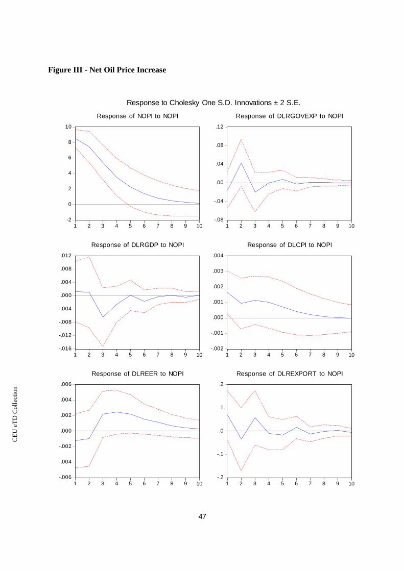
CE

UeT

DC

olle

ctio

n

47

Figure III - Net Oil Price Increase

-2

0

2

4

6

8

10

1 2 3 4 5 6 7 8 9 10

Response of NOPI to NOPI

-.08

-.04

.00

.04

.08

.12

1 2 3 4 5 6 7 8 9 10

Response of DLRGOVEXP to NOPI

-.016

-.012

-.008

-.004

.000

.004

.008

.012

1 2 3 4 5 6 7 8 9 10

Response of DLRGDP to NOPI

-.002

-.001

.000

.001

.002

.003

.004

1 2 3 4 5 6 7 8 9 10

Response of DLCPI to NOPI

-.006

-.004

-.002

.000

.002

.004

.006

1 2 3 4 5 6 7 8 9 10

Response of DLREER to NOPI

-.2

-.1

.0

.1

.2

1 2 3 4 5 6 7 8 9 10

Response of DLREXPORT to NOPI

Response to Cholesky One S.D. Innovations ± 2 S.E.

CE

UeT

DC

olle

ctio

n

48

Appendix IV – Variance Decomposition

Variance Decomposition of Inflation

Period Oil Price Shock Oil Price Shock+ Oil Price Shock- NOPI

Variance Decomposition of Inflation

1 0.311728 1.146070 0.003309 4.549059

(1.43030) (2.03376) (1.18588) (3.78968)

2 5.561239 3.779771 5.057495 4.747474

(4.25633) (3.85397) (3.84103) (4.08796)

3 9.931966 4.981928 9.439419 5.645376

(6.08004) (4.62248) (5.61965) (4.69063)

4 13.47622 5.701445 12.24556 6.401035

(7.31110) (5.16035) (6.73438) (5.30438)

5 16.25487 6.016011 13.49260 6.780646

(8.25007) (5.43976) (7.28999) (5.76928)

6 18.43269 6.146407 14.18726 6.885180

(9.02067) (5.58639) (7.61313) (6.07430)

7 20.11945 6.195915 14.48601 6.898371

(9.69155) (5.65128) (7.78980) (6.27664)

8 21.39509 6.216340 14.60566 6.892544

(10.2932) (5.68738) (7.88824) (6.41373)

9 22.32347 6.222317 14.65603 6.887535

(10.8377) (5.70624) (7.94591) (6.50575)

10 22.95757 6.224477 14.67237 6.885719

(11.3301) (5.71794) (7.97959) (6.57369)

Variance Decomposition of Real GDP Growth

Period Oil Price Shock Oil Price Shock+ Oil Price Shock- NOPI

CE

UeT

DC

olle

ctio

n

49

Variance Decomposition of Real GDP Growth

1 0.086450 0.102791 0.007701 0.070491 (1.22675) (1.19513) (1.09870) (1.21564)

2 0.628931 0.082050 0.096280 0.086438

(1.87390) (1.48576) (1.46579) (1.70187)

3 0.478509 1.554440 0.119678 1.322804

(1.81823) (2.64493) (1.79309) (2.45094)

4 0.448570 1.650624 0.259416 1.469451

(2.04477) (2.83531) (1.81828) (2.40591)

5 0.399021 1.628351 0.303684 1.449549

(2.23029) (2.80408) (1.81306) (2.37438)

6 0.371211 1.733216 0.322369 1.524522

(2.47734) (2.84439) (1.83326) (2.43166)

7 0.349867 1.759427 0.324801 1.523338

(2.75529) (2.87017) (1.83706) (2.43159)

8 0.336414 1.759707 0.330005 1.521757

(3.06336) (2.86428) (1.83817) (2.42811)

9 0.327310 1.763232 0.331626 1.525184

(3.38726) (2.86395) (1.84190) (2.43307)

10 0.321512 1.767003 0.331652 1.525422

(3.71830) (2.86845) (1.84345) (2.43478)

Variance Decomposition of Real Export

Period Oil Price Shock Oil Price Shock+ Oil Price Shock- NOPI

Variance Decomposition of Real Export

1 0.041911 1.321473 2.204719 1.373548

(1.20646) (2.12829) (2.70222) (2.07550)

CE

UeT

DC

olle

ctio

n

50

2 0.066922 0.934787 1.512672 1.120003

(1.67869) (1.97575) (2.38291) (2.08346)

3 2.529145 2.506141 2.563900 1.644638

(2.16800) (3.02407) (3.21426) (2.49552)

4 4.409824 2.968016 2.567906 1.588552

(2.76122) (3.38238) (3.21105) (2.37444)

5 6.399412 2.998096 2.588095 1.582290

(3.41068) (3.30897) (3.13699) (2.37023)

6 8.026013 2.988597 2.598031 1.615413

(4.01205) (3.30395) (3.16257) (2.41006)

7 9.345291 3.039239 2.611239 1.639893

(4.52338) (3.35117) (3.16333) (2.40579)

8 10.35860 3.062306 2.625273 1.637575

(4.94019) (3.35893) (3.16195) (2.40621)

9 11.12360 3.059849 2.622672 1.637577

(5.27885) (3.35665) (3.16209) (2.40869)

10 11.68706 3.061395 2.623177 1.641402

(5.55217) (3.36021) (3.16197) (2.40813)

Variance Decomposition of Real Government Expenditure

Period Oil Price Shock Oil Price Shock+ Oil Price Shock- NOPI

Variance Decomposition of Real Government Expenditure

1 0.130349 0.008318 0.004986 0.523949

(1.19442) (1.12570) (1.09756) (1.53938)

2 0.659369 0.005311 1.002031 2.887466

(2.09980) (1.53635) (2.19787) (3.23196)

3 0.841468 0.892630 4.945968 3.223399

(2.10375) (2.67348) (4.64484) (3.61041)

4 1.311099 1.325530 5.809501 3.207613

CE

UeT

DC

olle

ctio

n

51

(2.41774) (3.30651) (5.11072) (3.54672)

5 1.870726 1.349837 5.768389 3.237315

(2.68822) (3.37993) (5.06752) (3.50507)

6 2.466584 1.344686 5.772332 3.232938

(3.01616) (3.37481) (5.06785) (3.49603)

7 3.056159 1.352709 5.810090 3.234111

(3.34308) (3.38718) (5.08882) (3.48892)

8 3.579683 1.352911 5.812106 3.233940

(3.65882) (3.38725) (5.08710) (3.48095)

9 4.029328 1.352701 5.810244 3.232826

(3.95079) (3.38788) (5.08287) (3.47634)

10 4.393461 1.352689 5.810906 3.232659

(4.21929) (3.39009) (5.08338) (3.47510)

Variance Decomposition of Real Effective Exchange Rate

Period Oil Price Shock Oil Price Shock+ Oil Price Shock- NOPI

Variance Decomposition of Real Effective Exchange Rate

1 5.510344 5.246537 2.932171 0.431393

(4.04956) (3.93728) (3.08220) (1.83396)

2 3.762121 5.131976 2.854022 0.651821

(3.70148) (3.88786) (3.13063) (2.23955)

3 2.560136 4.990260 2.923911 1.874858

(3.12544) (3.86455) (3.25961) (2.44621)

4 2.052096 5.050694 2.965591 3.363883

(2.55257) (3.80259) (3.25499) (3.19965)

5 2.250101 5.082457 3.058450 4.552070

(2.50267) (3.78204) (3.23582) (3.84563)

6 3.051524 5.109379 3.170132 5.120399

CE

UeT

DC

olle

ctio

n

52

(3.13673) (3.77258) (3.23346) (4.21284)

7 4.294068 5.132799 3.251720 5.419231

(4.13028) (3.76898) (3.24271) (4.42163)

8 5.817758 5.137546 3.289844 5.532777

(5.21540) (3.76838) (3.25030) (4.53247)

9 7.491802 5.140742 3.310715 5.570435

(6.27314) (3.76866) (3.25743) (4.59433)

10 9.220781 5.142475 3.321230 5.585517

(7.26072) (3.76910) (3.26318) (4.63606)

Cholesky ordering: Specification of oil price shock, Inflation, Real GDP Growth, RealExport, Real Government Expenditure, Real Effective Exchange Rate.

Standard Errors: Monte Carlo (1000 repetitions)