Embed Size (px)
DESCRIPTION
By: Mark Bright and Mike Donaldson. Advisor: Dr. Gary Dempsey. Project Goal System Applications Thermal Plant Overview Engine Side Thermal Side. The goal of our Engine Control Workstation is to simulate thermal environments that are found in liquid-based cooling systems. - PowerPoint PPT Presentation
Citation preview

By:Mark Bright
and Mike Donaldson
Advisor:Dr. Gary Dempsey

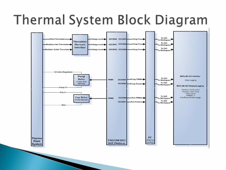
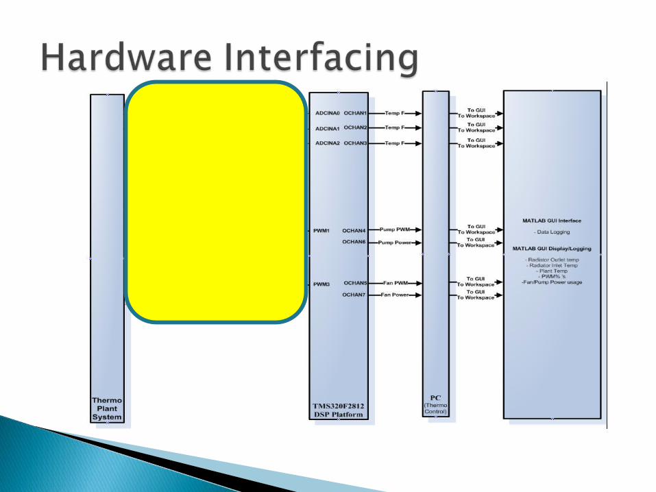
Project Goal System Applications Thermal Plant Overview
Engine Side Thermal Side

The goal of our Engine Control Workstation is to simulate thermal environments that are found in liquid-based cooling systems.
With this system we created several different control methods via MATLAB and Simulink working together to control both the engine and thermal transient and steady state responses.

Car Application PC Application
The overall goal of this project is to protect the motor with varying loads with minimum energy usage
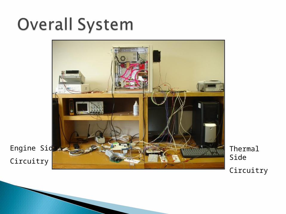
Engine Side
Circuitry
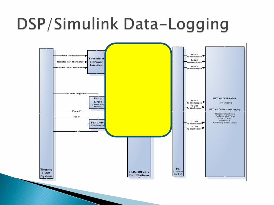
Thermal Side
Circuitry
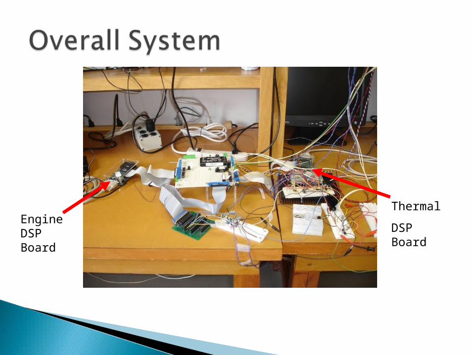
Engine DSP Board
Thermal
DSP Board

Generator
Thermistor
Flowmeter
Pump
Pittman
Motor
Cooling Blocks
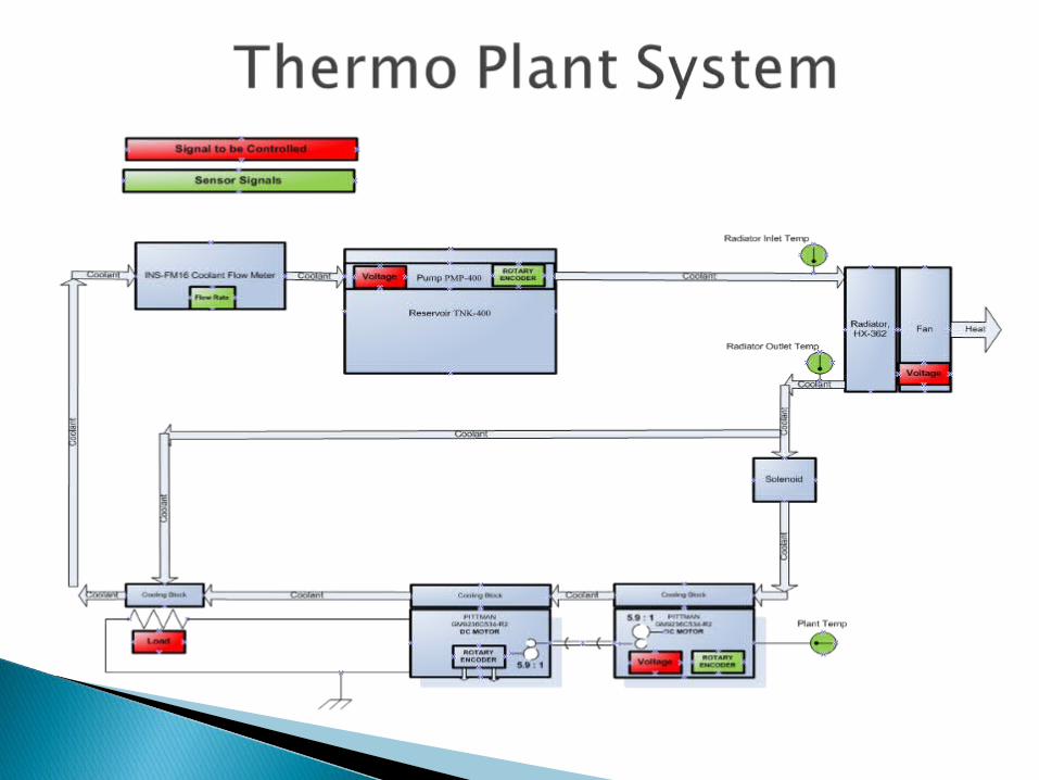


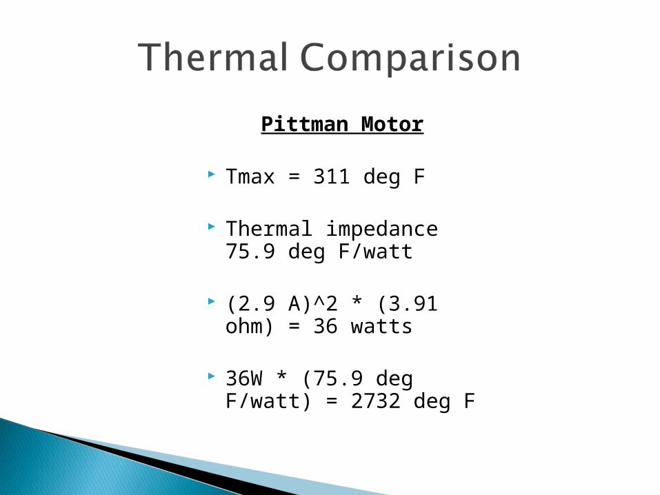
Pittman Motor
Tmax = 311 deg F
Thermal impedance 75.9 deg F/watt
(2.9 A)^2 * (3.91 ohm) = 36 watts
36W * (75.9 deg F/watt) = 2732 deg F

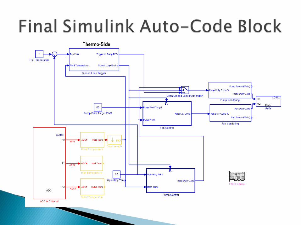
Engine Control:
Minimize C-code and execution time
Learn Auto-Code generation platform of Simulink/DSP interface
Design software for PWM generation and velocity calculation from rotary encoder.
Design closed-loop controllers for velocity and acceleration control.
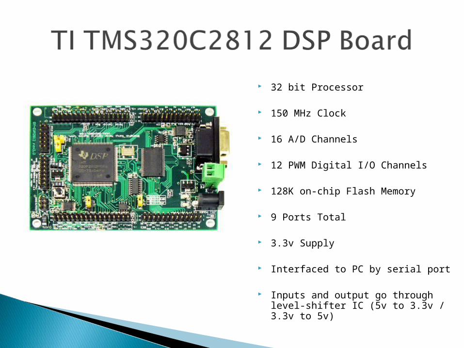
32 bit Processor
150 MHz Clock
16 A/D Channels
12 PWM Digital I/O Channels
128K on-chip Flash Memory
9 Ports Total
3.3v Supply
Interfaced to PC by serial port
Inputs and output go through level-shifter IC (5v to 3.3v / 3.3v to 5v)

User Interaction:Set RPM and
Gain
System Design Simulink Model
MATLAB GUI
Code Composer Auto Code Generated
C Code
TI 2812 DSP Board
PWM Output to Drive Motor
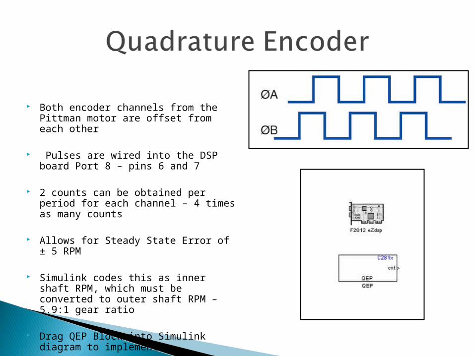
Both encoder channels from the Pittman motor are offset from each other
Pulses are wired into the DSP board Port 8 – pins 6 and 7
2 counts can be obtained per period for each channel – 4 times as many counts
Allows for Steady State Error of ± 5 RPM
Simulink codes this as inner shaft RPM, which must be converted to outer shaft RPM – 5.9:1 gear ratio
Drag QEP Block into Simulink diagram to implement
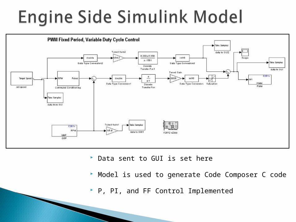
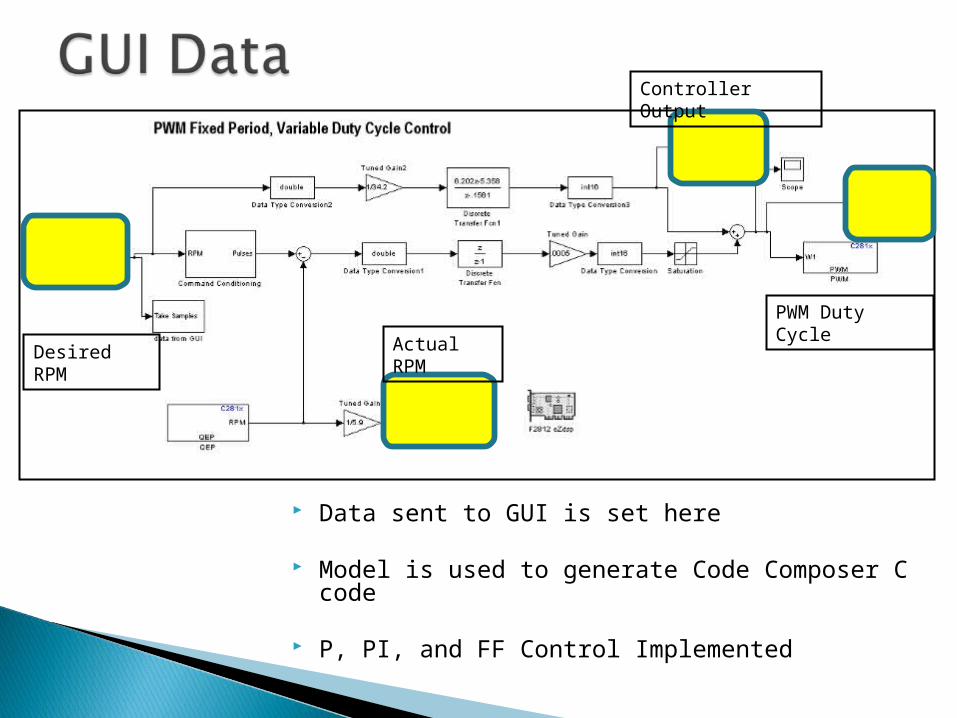
Data sent to GUI is set here
Model is used to generate Code Composer C code
P, PI, and FF Control Implemented

Data sent to GUI is set here
Model is used to generate Code Composer C code
P, PI, and FF Control Implemented

Data sent to GUI is set here
Model is used to generate Code Composer C code
P, PI, and FF Control Implemented

Data sent to GUI is set here
Model is used to generate Code Composer C code
P, PI, and FF Control Implemented

Data sent to GUI is set here
Model is used to generate Code Composer C code
P, PI, and FF Control Implemented
Data sent to GUI is set here
Model is used to generate Code Composer C code
P, PI, and FF Control Implemented
Desired RPM
Actual RPM
Controller Output
PWM Duty Cycle
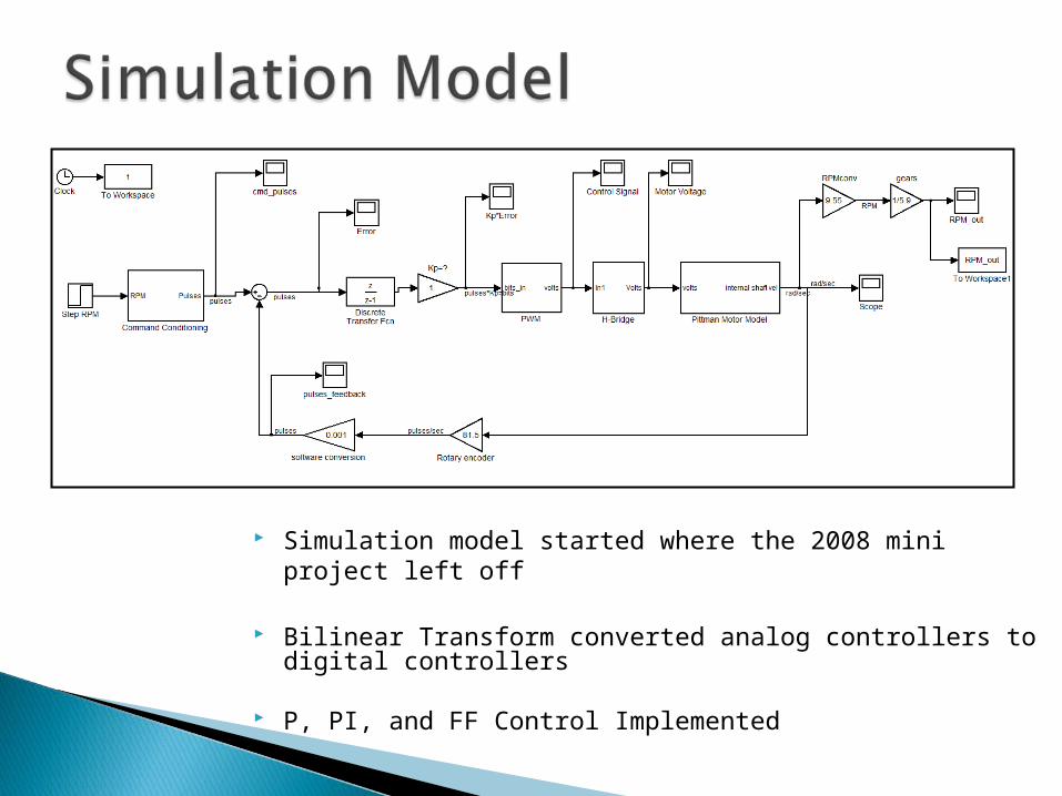
Simulation model started where the 2008 mini project left off
Bilinear Transform converted analog controllers to digital controllers
P, PI, and FF Control Implemented
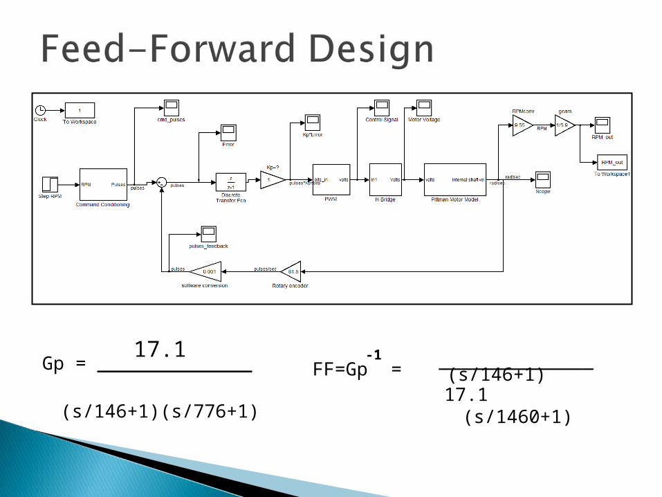
Gp = ______________ (s/146+1)(s/776+1)
______________
(s/146+1)
(s/1460+1)17.1FF=Gp =
17.1 -1
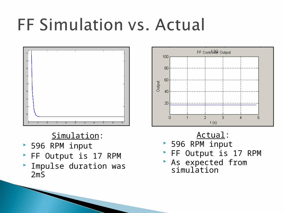
Simulation: 596 RPM input FF Output is 17 RPM Impulse duration was 2mS
Actual: 596 RPM input FF Output is 17 RPM As expected from
simulation
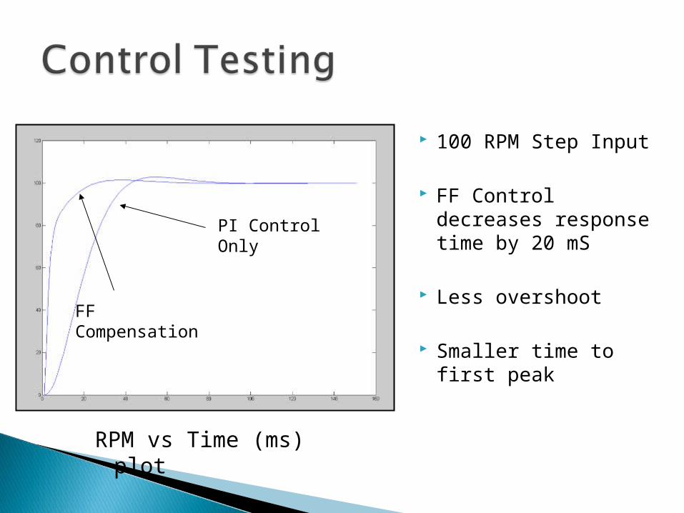
100 RPM Step Input
FF Control decreases response time by 20 mS
Less overshoot
Smaller time to first peak
FF Compensation
PI Control Only
RPM vs Time (ms) plot
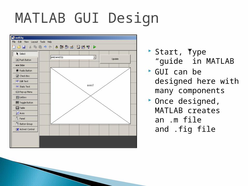
Start, Type “guide” in MATLAB
GUI can be designed here with many components
Once designed, MATLAB creates an .m file and .fig file
MATLAB GUI Design
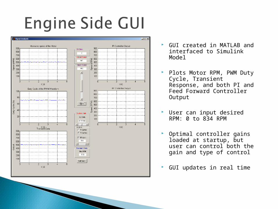
GUI created in MATLAB and interfaced to Simulink Model
Plots Motor RPM, PWM Duty Cycle, Transient Response, and both PI and Feed Forward Controller Output
User can input desired RPM: 0 to 834 RPM
Optimal controller gains loaded at startup, but user can control both the gain and type of control
GUI updates in real time
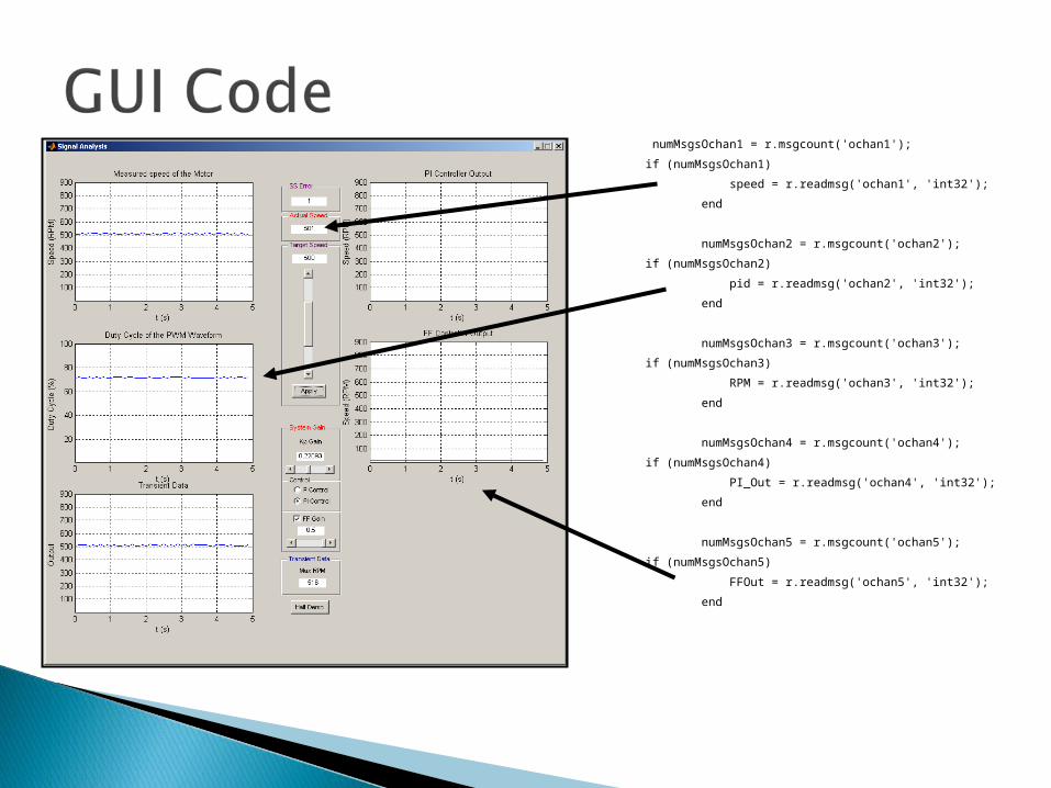
numMsgsOchan1 = r.msgcount('ochan1');
if (numMsgsOchan1)
speed = r.readmsg('ochan1', 'int32');
end
numMsgsOchan2 = r.msgcount('ochan2');
if (numMsgsOchan2)
pid = r.readmsg('ochan2', 'int32');
end
numMsgsOchan3 = r.msgcount('ochan3');
if (numMsgsOchan3)
RPM = r.readmsg('ochan3', 'int32');
end
numMsgsOchan4 = r.msgcount('ochan4');
if (numMsgsOchan4)
PI_Out = r.readmsg('ochan4', 'int32');
end
numMsgsOchan5 = r.msgcount('ochan5');
if (numMsgsOchan5)
FFOut = r.readmsg('ochan5', 'int32');
end

if ((numMsgsOchan1 ~=0) && (numMsgsOchan2 ~= 0) && (numMsgsOchan3 ~= 0) && (numMsgsOchan4 ~= 0) && (numMsgsOchan5 ~= 0))
axes(handles.axes3);
plot(handles.axes3,x_axis1, RPM);
title(handles.axes3,'Measured speed of the Motor');
xlabel(handles.axes3,'t (s)');
ylabel(handles.axes3,'Speed (RPM)');
grid(handles.axes3,'on');
axis(handles.axes3,[0 5 1 850]);
axes(handles.axes4);
cycle = double(pid);
plot(handles.axes4,x_axis1, cycle);
title(handles.axes4,'Duty Cycle of the PWMWaveform');
xlabel(handles.axes4,'t (s)');
ylabel(handles.axes4,'Duty Cycle (%) ');
grid(handles.axes4,'on');
axis(handles.axes4,[0 5 1 100]);

Acceleration Control
◦ Adjustable Feed Forward control with different types of input commands: combos of ramps, steps, and parabolic. Load changes can simulate hills and different road conditions.
CAN Bus Interface
◦ Use the DSP board’s CAN bus to send data between the boards. This would allow for a main GUI to control both sides of the system.
Data Logging Feature
◦ Allow for a user to tune controllers and compare results. Could implement a new EE431 / 432 homework or design project around the system.
Set Control Points for Thermal and Engine Response
◦ Set desired temperature for a change in the coolant as well as a engine RPM governor based on load conditions

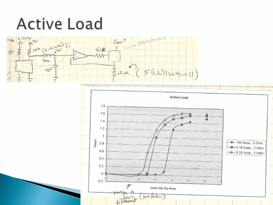
Variable Resistance
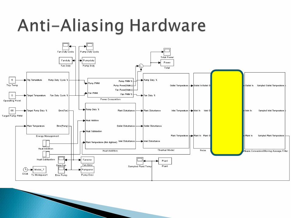
Anti-aliasing filter

Use PWM to drive Pump/Fan
Interface from digital to analog
Average Voltage seen by the device

Opto-Isolator
TIP120 choice
Design for 3A Opto-Isolator

LPF to ‘DC’ the PWM
Ideal Op Amp theory
Voltage @ Input = Voltage @ Pump
Opto-Isolator

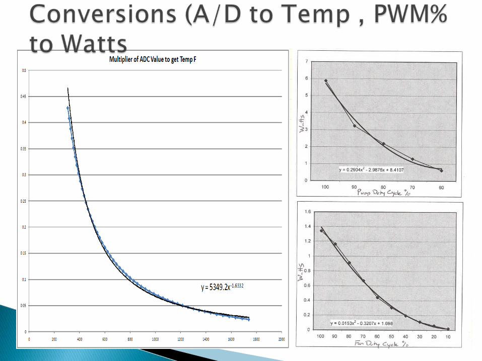
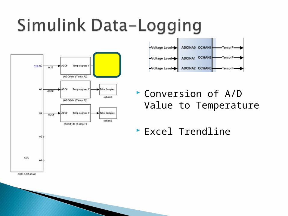
Conversion of A/D Value to Temperature
Excel Trendline
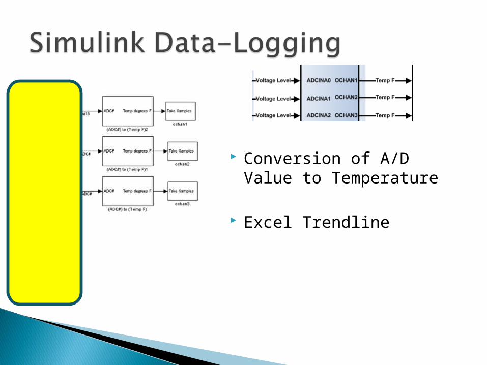
Conversion of A/D Value to Temperature
Excel Trendline

Conversion of A/D Value to Temperature
Excel Trendline
Conversion of A/D Value to Temperature
Excel Trendline
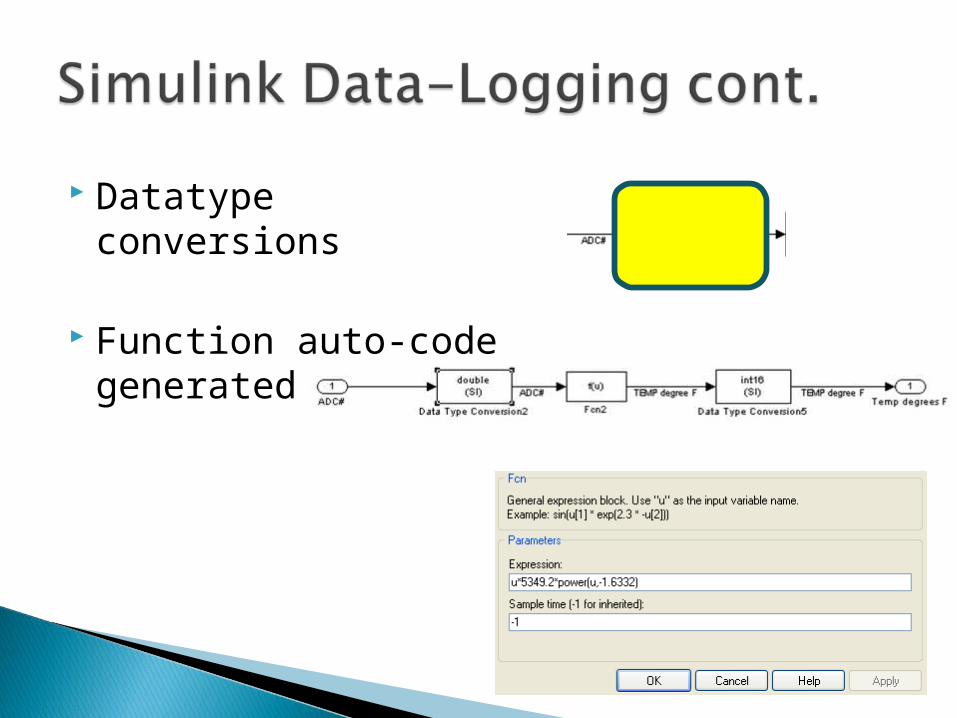
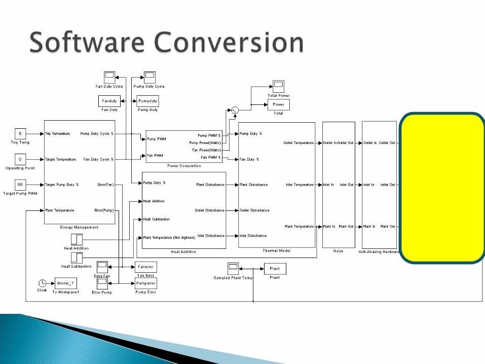
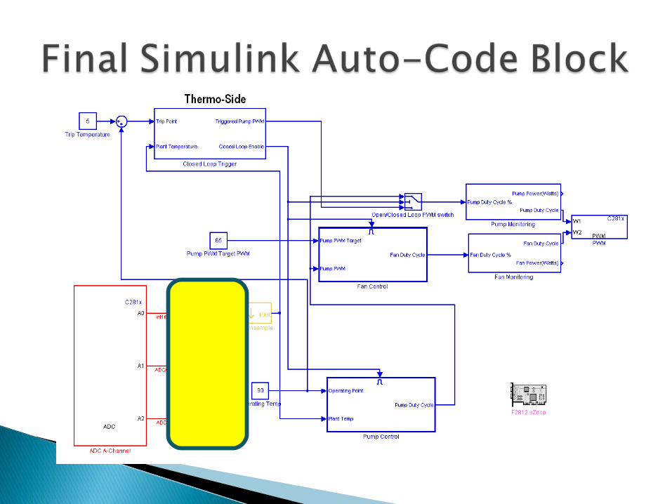
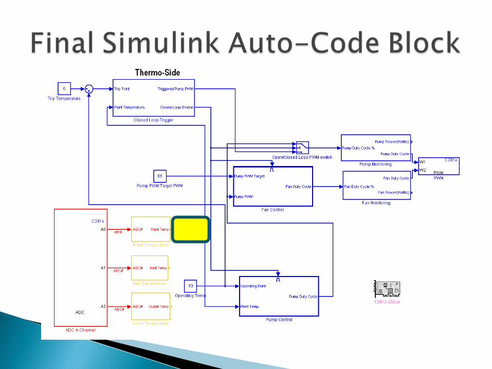
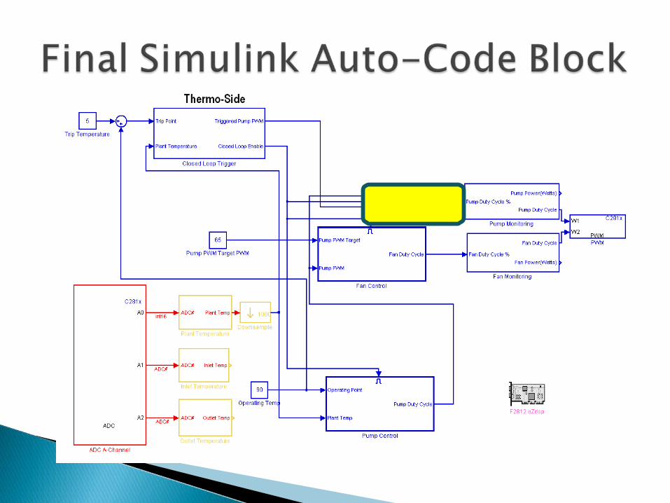
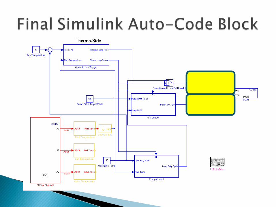
Datatype conversions
Function auto-code generated

Datatype conversions
Function auto-code generated


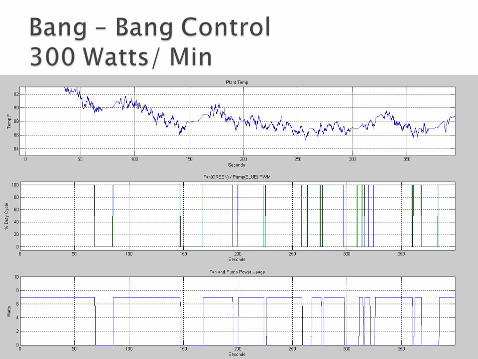
Bang – Bang
Improved Bang Bang
P Control
PI Control


Fan PWM %
Pum
p P
WM
%
0 10 20 30 40 50 60 70 80 90 10060
65
70
75
80
85
90
95
100
-5.5
-5
-4.5
-4
-3.5
-3
-2.5
-2
-1.5
-1
-0.5
0
Pum
p P
WM
%
Fan PWM%

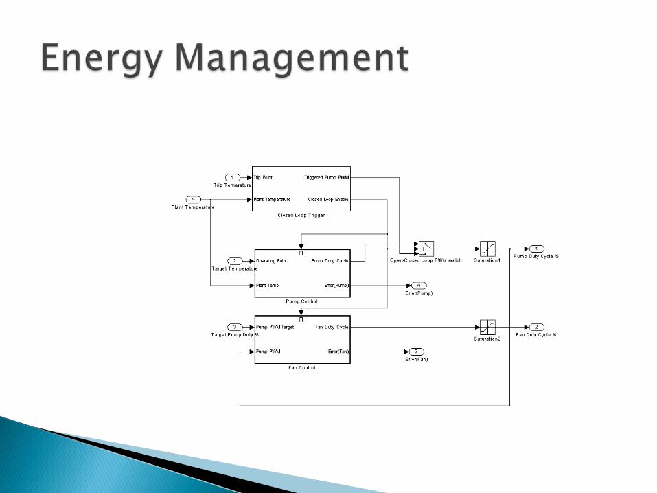
Supervisory Control
Further improvement by utilizing Pump and Fan cooling efficiencies
Faster PID Control
Use of more temperature sensors
Use of CAN bus
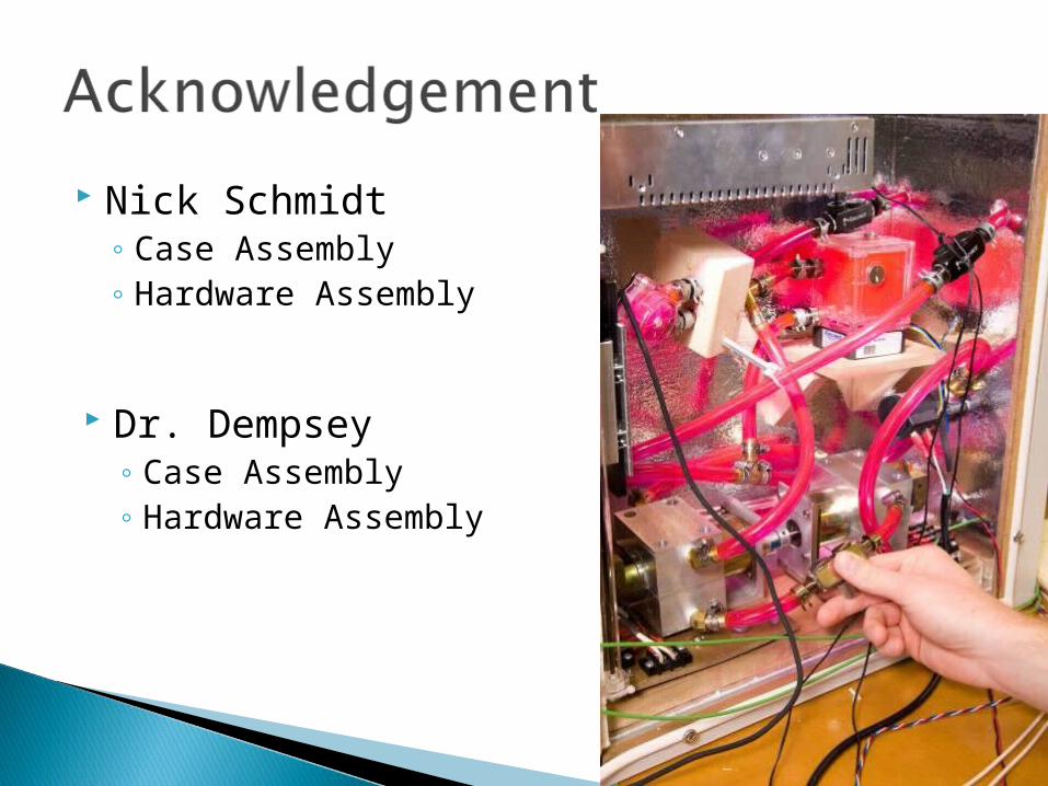
Nick Schmidt◦ Case Assembly◦ Hardware Assembly
Dr. Dempsey◦ Case Assembly◦ Hardware Assembly


Plant Wc is at 899 rad/sec
P Control System Wc was at 164 rad/sec
Gain = .08
Phase Margin with P control:◦ 115
Gp = __________________ (s/146+1)(s/776+1)
17.1


Gp(s) =K * 1/(Tc(s)+1) * e^-(s)Td
Pump/Plant ◦ K = (-.8 degrees F / 6.4 V)◦ Tc = 20◦ Td = 6
Fan/Plant◦ K = (-9.6 degrees F / 13V)◦ Tc = 12◦ Td = 15
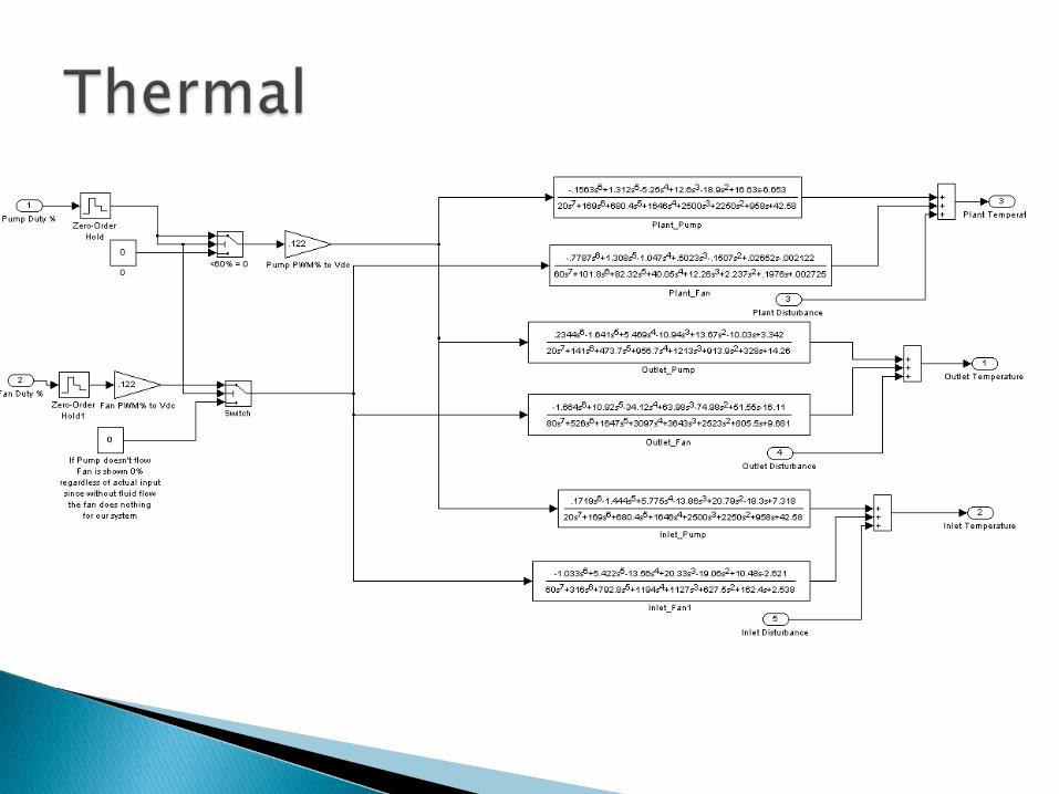
Thermal Transfer Functions
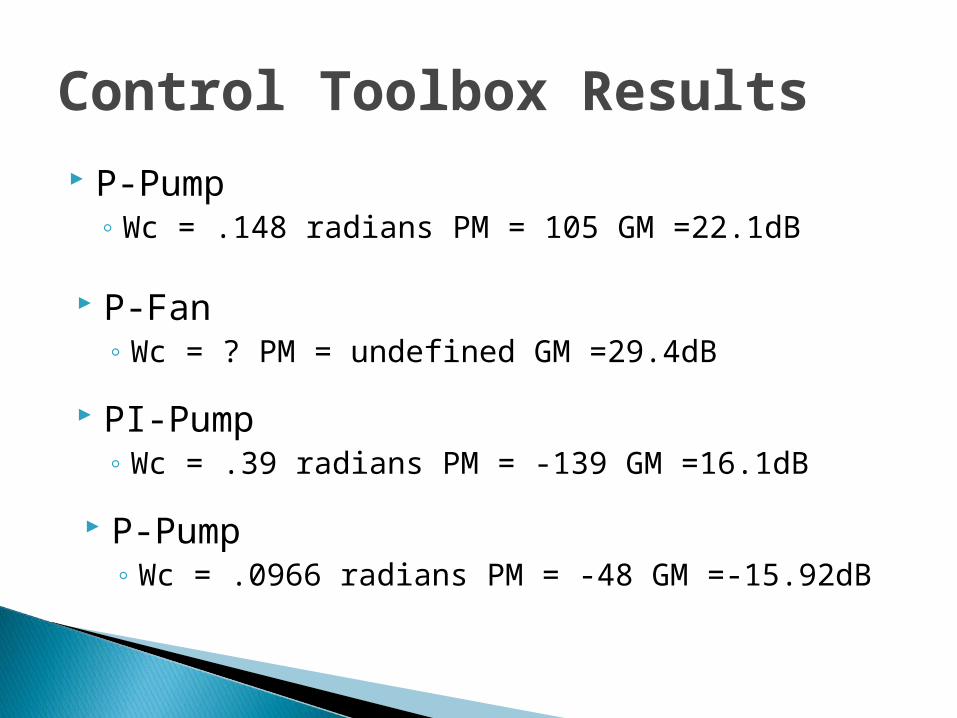
Control Toolbox Results P-Pump
◦ Wc = .148 radians PM = 105 GM =22.1dB
P-Fan◦ Wc = ? PM = undefined GM =29.4dB
PI-Pump◦ Wc = .39 radians PM = -139 GM =16.1dB
P-Pump◦ Wc = .0966 radians PM = -48 GM =-15.92dB
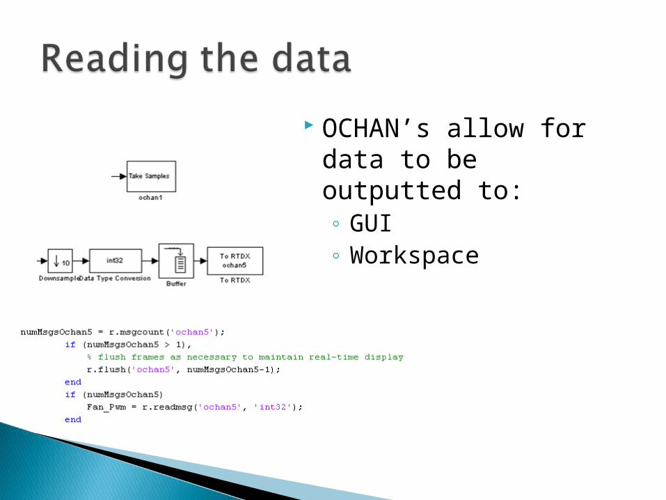
OCHAN’s allow for data to be outputted to:◦ GUI◦ Workspace

PWM Brush Type Servo Amplifer – Model 10A8DD
Protected for over-voltage and over-current
DC Supply Voltage: 20-80v
Peak Current: ±10A Maximum Continuous
Current: ±6A