Embed Size (px)
Citation preview
BARGAINING OVER SONS AND DAUGHTERS:CHILD LABOR,SCHOOL ATTENDANCE AND INTRA-HOUSEHOLD GENDER
BIAS IN BRAZIL
by
Patrick M. Emerson and André Portela Souza
Working Paper No. 02-W13
May 2002
DEPARTMENT OF ECONOMICSVANDERBILT UNIVERSITY
NASHVILLE, TN 37235
www.vanderbilt.edu/econ
Bargaining over Sons and Daughters:Child Labor, School Attendance and Intra-household Gender
Bias in Brazil
Patrick M. EmersonDepartment of Economics
University of Colorado at DenverDenver, Colorado 80217
André Portela SouzaEconomics DepartmentVanderbilt UniversityNashville, TN 37315
May 2002
Abstract
This paper we examine intra-household gender differences and the incidence of child labor andchildren’s school attendance in Brazil to test whether the unitary model of household allocations is suitablein the child labor context. We begin by building an intra-household allocation model where fathers andmothers may affect the education investment and the child labor participation of their sons and daughtersdifferently due to differences in the children's human capital technologies and/or differences in parentalpreferences. Using the 1996 Brazilian Household Survey, we estimate the impact of a parent’s education,non-labor income and child labor experience on the labor market status and school attendance of their sonsand daughters separately. We find that, for children’s labor status, the father’s education, non-labor incomeand the age at which he first began working in the labor market has a greater impact on the labor status ofsons than of daughters, while the opposite is true for mother’s education, non-labor income and the age atwhich she first began working in the labor market, which have a greater impact on the labor status ofdaughters than of sons. In addition, when it comes to schooling decisions, both fathers and motherseducation and non-labor income appear to have a greater positive impact on sons than on daughters.
(JEL Classification Numbers: J20, O12, O54)
(Keywords: Child Labor, Brazil, Intra-Household Allocations, Bargaining Models,Gender Bias)
Acknowledgements: For valuable comments and advice, we would like to thank Francine Blau,Lawrence Khan, John Abowd and Kaushik Basu. This paper benefited from presentations at the 2001Western Economics Association International Meetings, at the 2001 Latin American and CaribbeanEconomic Association Meeting, at 2001 Northeast Universities Development Consortium Conference, andat the University of Colorado at Denver.

1
Bargaining over Sons and Daughters:
Child Labor, School Attendance and Intra-household Gender Bias in Brazil
This paper uses an extensive survey dataset of Brazilian households to examine if
evidence exists that there is bargaining between mothers and fathers in the decision to
send their sons and daughters to work in the labor market and to school, and explores the
possibility that there exists intra-household gender bias in these decisions. The objective
of the paper is to test the assumption of the unitary model of intra-household allocations
in the child labor context and the assumption that sons and daughters are treated similarly
when fathers and mothers make these work and schooling decisions.
The recent child labor literature generally assumes (ala Becker, 1982) that parents
have common preferences and are altruistic toward their children (e.g., Baland and
Robinson, 2000; Bell and Gersbach, 2000; Dessy, 2000; Emerson and Portela, 2000;
Basu and Van, 1998). Additionally, the empirical literature on child labor has
predominantly explored the relation between the economic conditions and incentives of
the family unit and the child labor outcomes (e.g. Emerson and Portela, 2000; Ray, 2000;
Grottaert and Patrinos, 1999; Jensen and Nielsen, 1997). Although a unitary model of
intra-household allocations is a valid starting point in order to focus on the poverty
dimension of child labor, this emphasis does not account for other factors of potential
importance. Recently, a few studies have examined intra-household allocations
explicitly. For example, Basu (2001) and Ridao-Cano (2000) extend intra-household
behavior to child labor decisions. Both authors suggest that fathers and mothers have
different impacts in the labor supply of their children, and that this is potentially related
2
to their relative bargaining power. Neither, however, explore gender bias within the
intra-household allocation decisions.1
There is also an extensive literature on gender differences in human capital
investments and outcomes that has presented some evidence of intra-household gender
bias. Sen (1990), for example, reports that female mortality rate is significantly higher
than those for men in Asia and North Africa. Others studies have shown that sons are
favored in the intra-household allocation of nutrients and have better anthropometric
outcomes (e.g. Behrman, 1988; Sen, 1984).
Perhaps even more compelling are recent studies that have found that the gender
bias in the children’s inputs or outcomes is related to the gender of the parent who
controls the distribution of these resources. In a study of families in the U.S., Ghana and
Brazil, Duncan Thomas (1994) finds that children’s health achievement (as measured by
height for age) is linked to the educational attainment and non-labor income of the parent
of the same sex as the child. In other words, sons do better (are taller) the more education
and non-labor income the father has and daughters do better the more education and non-
labor income of the mother. This finding suggests that there may be differences in the
preferences of the parents and/or that there may be technological differences in child
rearing. Moreover, it supports the rejection of the unitary family model that assumes
parents have common preferences and pool their resources. In fact, there is some
additional evidence that the unitary family model hypothesis is not consistent with
Brazilian data. Thomas (1990) shows that unearned income controlled by mothers has
stronger impacts on family’s health than income under father’s control. In addition,
Tiefenthaler (1999) finds that family labor supply decisions in Brazil do not conform to
1 Basu’s theoretical contribution goes further to include the possibility that the choices taken by the
3
the implications of the unitary family model. None of these studies, however, examine
intra-household gender bias in the child labor context.
In a previous paper (Emerson and Portela, 2000) we found strong evidence of
inter-generational persistence in child labor among families in Brazil. Specifically, we
found that people who start work at a younger age end up with lower earnings as adults,
and that children are more likely to be child laborers the younger their parents were when
they entered the labor force, and the lower the educational attainment of their parents as
well as their grandparents. These findings are consistent with unitary models of child
labor and poverty persistence (see e.g., Bell and Gersbach, 2000; Dessy, 2000; Emerson
and Portela, 2000; Basu, 1999; Glomm, 1997) where parent’s child labor hampers their
ability to gain human capital through schooling which makes them unable to command a
high enough wage as an adult to afford to keep their children out of the labor force.
However, and what is important to the current paper, these results also held when
we performed the analysis for sons and daughters separately. That is, there is a
persistence of child labor from parents to sons as well as from parents to daughters. This
begs the question, is this effect different for sons and daughters based on the schooling,
non-labor income and child labor experience of their mothers and fathers?
In the present study, we investigate the impact of fathers and mothers attributes on
the child labor and school attendance of their sons and daughters, separately. In line with
the existing child labor literature, we assume altruistic parents make the decision to send
children to work, but we allow for parental preferences to differ across children as well as
allowing the technology that converts education into human capital to vary across
children. Using Brazilian household survey data, we estimate the impact of a parent’s
individuals can affect their bargaining power.
4
education, non-labor income and child labor experience on the labor market status and
school attendance of their sons and daughters separately. We find compelling evidence
that, for children’s labor status, the father’s education, non-labor income and the age at
which he first began working in the labor market have a greater impact on the labor status
of sons than of daughters, while the opposite is true for mother’s education, non-labor
income and the age at which she first began working in the labor market, which have a
greater impact on the labor status of daughters than of sons. Equally compelling, when it
comes to schooling decisions, both fathers and mothers education and non-labor income
appear to have a greater positive impact on sons than on daughters.
This paper proceeds as follows: The next section presents a simple model of
household allocations. It illustrates the argument that altruistic fathers and mothers may
have different impacts on their sons and daughters outcomes due to differences in their
preferences and/or differences in the children’s human capital technologies. Section
three describes the data used in this paper and the variables used in the regression
estimations. Section four presents and discusses the empirical results and section five
summarizes the main findings and discusses policy implications.
II. The Model
In order to model household allocations where parents have different preferences,
it is necessary to depart from the unitary family model. Two classes of models typically
used in the intra-household allocation literature that allow differences in parents'
preferences are the family bargaining model (see, e.g., Lundberg and Pollak, 1993;
McElroy, 1990; McElroy and Horney, 1981) and the collective model (e.g., Chiappori,
1992, 1988). Bargaining models assume that the household allocation outcomes are the
5
result of a bargaining process in which household members seek to allocate resources
they control to goods they individually prefer. The resulting equilibria are sensitive to
the threat point definition and equilibrium concept assumed. The collective model leaves
unspecified the underlying nature of the allocation process within the household but
assumes that the resource allocations are Pareto efficient.2 Due to its generality, we opt
to use this collective approach to household decisions to motivate our discussion and the
empirical investigation that follows.
Consider a household consisting of two heads (mother and father) and n children
who can be sons or daughters. Both fathers and mothers are altruistic in that they value
the consumption of each member of the household and the human capital achievement of
their children. The children in the household can go to school, go to work or spend time
in both activities. The amount of schooling children receive determines the wage they
are able to command as adults, and children who work are not able to get as much
education as those who do not. Therefore the amount of labor income the father and
mother bring into the household depends on how much schooling they received as
children. Thus parents who were child laborers command lower wages and are more
likely to demand that their children work to supplement the family income. This is what
we term the inter-generational persistence of child labor.
Browning and Chiappori (1998) postulate that for all Pareto-efficient allocations,
there exist a set of weights such that the household welfare function can be represented
by a linear combination of father’s and mother’s utilities, where the weights on each
person’s utility reflects their bargaining power in the household. This power may be a
2 For a summary of intra-household allocation models, see Behrman (1997) and Strauss and Thomas(1995).
6
function of (among other things) the exogenous non-labor income they bring into the
home, and is a topic we explore in the empirical section of this chapter.
Consider a general household’s utility maximization problem:
Umax = +);,,,,,,,,,,,( 11 fnmfnpmff znhhllcccccu LLλ
);,,,,,,,,,,,()1( 11 mnmfnpmfm znhhllcccccu LLλ− (1)
Subject to the budget constraint:
∑∑==
++−+−+−≤+++n
jmfcjmmff
n
jjpmf IIwewlwlcccc
11
)1()1()1( (2)
Where U is the household’s welfare function, uf is the father’s utility function, um is the
mother’s utility function. The parameter λ represents the relative bargaining power in the
household and ]1,0[∈λ . The total consumption of the household is the sum of the
father’s consumption of his private goods, cf, the mother’s consumption of her private
goods, cm, the household’s consumption of public goods, cp, and the sum of each child j’s
consumption of his/her private good: njc j ,,1, L= . The consumption of leisure for the
father and mother are lf and lm, respectively. Parents also care about the human capital
achievement of their children, h1, … , hn, as well as the number of children in the
household, n.3 The terms zf and zm represent any individual, household and community
characteristics that effect the father’s and mother’s utility respectively. The current wage
rates for the father, mother and children are given by wf, wm, and wc, respectively.
Additionally, fathers and mothers may have exogenous non-labor income of their
own and these are given by If and Im. Finally, child j’s time spent in school (education) is
7
given by ej. Each person is endowed with one unit of time. For adults this time is split
between labor and leisure, so time spent working is 1-l. For children time is split
between working and going to school, so for them, time spent working is 1-e.
For ease of exposition we assume that the wages of the father and mother are
given by their production functions wf = hf and wm = hm, we normalize the child wage to
one, wc = 1, so a child who only works will earn a total of 1 unit of income. In order to
focus on parents' preferences and children's outcomes, we also assume that both fathers
and mothers value equally any additional unit of consumption regardless of the recipient
and that there does not exist a public good (cp = 0), so: Cccccn
jjpmf =+++ ∑
=1
.
Additionally, we assume that fathers and mothers supply labor inelastically or, in other
words, they spend all of their time working: lf = lm =0, that fertility is exogenous, and that
the utilities are monotonically increasing in consumption, so non-satiation applies.4
Children’s education is converted into adult human capital by the idiosyncratic
technology:
),;( mfjjj hhefh = , j∀ (3)
where 1)0( =jf , 0),;(
>∂
∂
j
mfjj
e
hhef, 0
),;(>
∂∂
f
mfjj
h
hhef, and
0),;(
>∂
∂
m
mfjj
h
hhef. This technology is different for each child because of different
abilities, societal bias (e.g. due to gender), etc. The father and mother’s human capital
3 h1, … , hn are the human capital levels children attain when they become adults and thus determine theiradult wage. To keep notation as simple as possible, time subscripts have not been used, but it is importantto note that this is what creates the intergenerational link in this model.4 The assumption that the two parents supply labor inelastically is not very realistic. However, it does noteffect the main prediction of the model that the son’s and daughter’s child labor incidence and humancapital attainment depend on each parent’s level of human capital and non-labor income. Thus, to keep theanalysis as simple as possible, this assumption will be maintained throughout the analysis.
8
also enters into the technology because of, among other things, the fact that the
effectiveness of children’s schooling depends critically on the pool of human capital at
home.5 The father’s and the mother’s human capital enter separately because there may
be differences in the way that parents interact with children depending on ability, gender,
birth order, etc.
With these assumptions in place, the household’s problem becomes:
Umax = +λ );,,,( 1 fnf zhhCu L );,,,()1( 1 mnm zhhCu Lλ− . (1’)
Subject to the budget constraint:
∑=
++−++=n
jmfjmf IIehhC
1
)1( (2’)
and the technology, (3). Substituting the constraint and technology directly into the
utility function of the household gives us the new household’s problem:
Unee },,{ 1
maxL
= +++−++λ ∑=
));,;(,),,;(,)1(( 111
fmfnnmf
n
jmfjmff zhhefhhefIIehhu L
));,;(,),,;(,)1(()1( 111
mmfnnmf
n
jmfjmfm zhhefhhefIIehhu L∑
=
++−++− λ (4)
If we assume an interior solution (ej > 0, j∀ ), we can derive the first-order conditions.
For each child j, the first order condition is:
je
U
∂∂
: 0)1()1()1( =
∂∂
⋅∂∂
+−∂∂
λ−+
∂∂
⋅∂∂
+−∂∂
λj
j
j
m
j
m
j
j
j
f
j
f
e
f
f
u
e
u
e
f
f
u
e
u(5)
It is worthwhile interpreting these first-order conditions before we move on. Note that in
the first set of brackets in equation (5), the father’s marginal utility of increasing child j’s
education is represented. It has two components: the first term is the loss of utility of the
father due to the foregone income of child j. The second term is the gain in utility due to
5 This is a similar assumption as that in Bell and Gersbach (2000) and Glomm (1997).
9
the increase of human capital of the child, which the father cares about. The second set
of brackets contains the same for the mother. Again, though the parent cares about the
child’s human capital attainment, the child does not see the benefit of such until he or she
reaches adulthood.
Deriving the first-order condition for each child, gives us a system of n equations
and n unknowns. Assuming the utility functions of the father and mother are well-
behaved, the optimal solution to this problem is a vector of education levels for each
child in the household that solve the n first-order conditions, *),*,(* 1 neee L= , where:
),,;,,,(~* mfmfmfjj zzIIhhee λ= . (6)
Of course, the child labor function is just 1- e*. The resulting adult human capital
of the household’s children is given by the function:
],);,,;,,,([* mfmfmfmfjjj hhzzIIhhefh λ= . (7)
The empirical implications of this model come from the comparative statics of
these two functions.
First, note that the higher the parents’ human capital attainment, the less needed is
the child’s contribution to current household consumption. This allows the children to
get more education and, as a result, they will be less likely to send their children to school
when they become adults. This is the essence of the persistence in child labor explored in
Emerson and Portela (2000). The focus of this paper is on the differential effects of
fathers and mothers on the child labor incidence and education of their sons and
daughters. This can be seen through an analysis of the optimal education and human
capital functions.
For simplicity, consider a four-person household that consists of a father, mother,
son and daughter. Now consider an increase, ceteris paribus, in the father’s human
10
capital. The effect on the son’s optimal education function is twofold: First, there is the
direct effect that more human capital for the father means more income for the family and
thus the family needs the son to provide less income, and this reduces the amount of child
labor. The reduction in child labor means more schooling and thus more human capital
of the son, which the family values. Second, more human capital of the father increases
the return to the son’s education through the technology that creates human capital from
education. The family will have, therefore, an increased incentive to invest more in the
son’s education.
The effect of the increase of the father’s human capital need not be, and in general
is not, the same for all kids. First, note that this would reduce child labor equally across
children, ceteris paribus, if additional schooling increases children's human capital
equally. But if additional schooling affects children's acquisition of human capital
differently, the child labor reduction would vary across children. Thus, the increase in
schooling will differ across the two kids due to their idiosyncratic human capital
technologies. Second, the increase in the father’s human capital may also affect the
marginal returns to education of the son and daughter differently. Third, the father may
favor one child over the other and his additional human capital may provide him stronger
bargaining power to impose his preferences. These differences can lead to different
investments in education (and, therefore, human capital) for the son and daughter of the
family.
Thus, the idiosyncratic nature of the human capital technology and parental
preferences that vary across children can lead to different impacts of each parent on the
same child as well as different parental impacts across children. For example, it is
possible that, for the same child, an increase in the father’s human capital will have a
11
different impact than an equal increase in the mother’s human capital. In addition, it
could be that the effect of an increase in mother’s human capital could be different for the
son and daughter. Finally, note that these differential impacts can also be driven by
different parental preferences over the human capital of their children and the relative
bargaining power of the father and mother.
It is precisely these differences that we explore in the empirical investigation of
the paper in section four. First, however, we describe the data used in the paper in the
next section.
III. The Data
The data used in this study come from the 1996 Brazilian Household Surveys
called Pesquisa Nacional por Amostragem a Domicilio (PNAD) conducted by Instituto
Brasileiro de Geografia e Estatística (IBGE), the Brazilian census bureau. It is an annual
labor force survey much like the Current Population Survey in the U.S. Covering all
urban areas and the majority of rural areas in Brazil (with the exception of the rural areas
of the Amazon region), the sample is based on a three stage sampling design. With the
exception of the first stage, the sampling scheme is self-weighted and the sampling varies
across regions and over time. The 1996 PNAD encompasses approximately 85,000
households.
The sample selection of this study consists of individuals between 10 and 14 years
old that are considered a son, daughter or other relative in the family unit.6 Each
observation consists of information on the child characteristics, his or her parent
6 PNAD assigns each individual to a position or ‘condition’ in the family. They are: (i) person of reference;(ii) spouse; (iii) son or daughter; (iv) other relative; (v) aggregate; (vi) pensionist; (vii) domestic worker;and (viii) relative of the domestic worker.
12
characteristics and his or her family characteristics. Since we are primarily concerned
with the impact of both parent’s education, non-labor income and child labor status on
the child labor status and schooling of the children, we use a sample of observations with
complete information of the father’s and the mother’s characteristics. Due to this
criterion, families with single heads are excluded from the analysis.7 Finally, all
observations for which the age difference between the head of the family or spouse, and
the oldest child is fourteen or below, are excluded as well.
The child labor variables for the children are constructed as follows. A child is
considered working if he or she worked on the labor market any strictly positive hours
per week.8 Moreover, a child is considered to work full time if he or she worked 20
hours or more on the labor market per week. Both definitions of child labor will be used
to check the robustness of the results. For each child, we also obtained his or her school
attendance status, gender and region of residence.
For the parents, we constructed a variable for the total years of schooling for each,
their non-labor income, their ages and current employment status. Additionally we
created a variable for the age at which they first started working in the labor market. We
also constructed a child labor indicator variable for mothers and fathers which is defined
as follows: The PNAD survey asks each individual the age at which he or she started to
work. A parent who responded that they began working in the labor market at 14 years
old or below is considered to have been a child laborer. Again, we will also use an
alternate definition where we consider an adult to have been a child laborer if they
entered the labor force at age 10 or below to check the robustness of the results and to
7 This selection criterion may impose some selection bias if, for example, children in single head familiesare more likely to work. Since we want to capture separate impacts of the father and the mother’sschooling, non-labor income and child labor status on sons and daughters, we use the sample with twoparent households.

13
account for any generational differences in child labor norms. Table A1 in the Appendix
presents the basic statistics of all the variables used in this analysis.9
IV. The Results
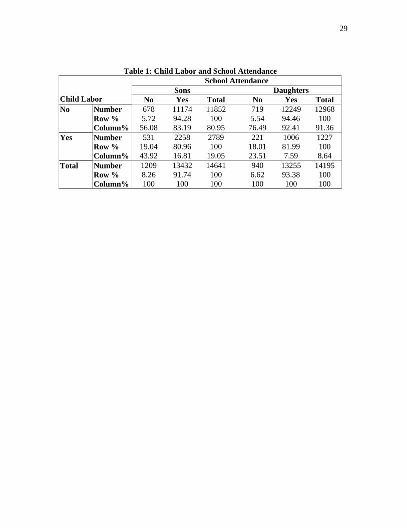
Child labor is widespread in our sample of households in Brazil. Table 1 shows
the incidence of child labor and schooling among the sons and daughters. Roughly 19
percent of all sons work some hours in the labor market, as do approximately 9 percent of
daughters. School attendance is also quite high with almost 92 percent of sons and over
93 percent of daughters attending school at least part-time. What is particularly
interesting (and important for the estimation strategy) is that among child laborers almost
81 percent of sons and 82 percent of daughters attend school as well.
In order to test the impact of intra-household gender differences on the child labor
and educational outcomes of children, we estimate a series of bivariate probit models.
The advantage of using the bivariate probit model in this case is that, because the child
labor and child schooling decisions are likely related as evidenced by the high proportion
of children that both work and go to school in the sample, it allows us to utilize the
information from the correlation among the errors of the child labor regression and the
child schooling regression.
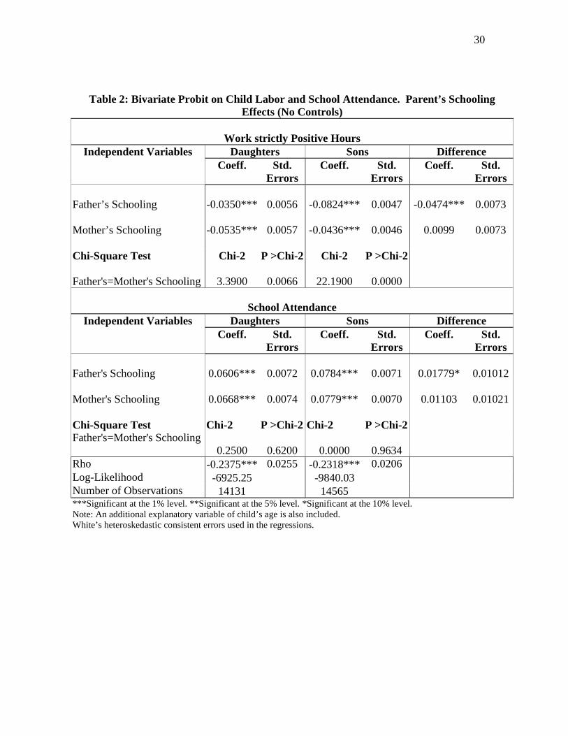
The first bivariate probit model we estimate is a regression of the child labor
indicator variable (for daughters and sons separately) and the child school indicator
variable on the father’s and mother’s years of schooling, controlling for child’s age.
Table 2 presents the results. The coefficient estimates suggest that the higher the parent’s
8 PNAD asks the usual hours worked per week for each individual working during the survey week.9 All results presented in this paper come from the un-weighted sample. We replicated all of the empiricaltests in this paper using a weighted sample and obtained qualitatively the same results.

14
schooling, the less likely to work and the more likely to attend school is the child.
However, fathers’ and mothers’ schooling have different impacts on sons’ and daughters’
labor participation and schooling. A mother’s education has a stronger negative effect on
a daughter’s probability to work relative to a father’s, whereas a father’s education has a
stronger negative impact on a son’s likelihood to work compared to a mother’s. The third
row of the first panel of Table 2 presents the Chi-square tests for the parents’ schooling
coefficients, which confirm these results. These tests reject the hypothesis that a father’s
and a mother’s schooling have same impact on a son’s (or daughter’s) probability to
work. The last two columns present a test of the difference between the parents’
schooling coefficients on a son’s probability of working and on a daughter’s probability
of working. Here, the results demonstrate that a father’s education has a stronger and
significantly negative impact on a son’s probability of being a child laborer compared to
the impact on a daughter’s. Conversely, a mother’s education has a stronger negative
impact (although not significant) on a daughter’s probability of working compared to a
son’s.
The panel in the bottom of Table 2 presents the results for school attendance. It
shows a father’s and mother’s education levels do not have different impacts on a
daughter’s probability to attend school. Additionally, a father’s and a mother’s education
do not have different impacts on a son’s probability of attending school. However, it
appears that the schooling of fathers and mothers has stronger positive impacts on a son’s
likelihood to attend school relative to a daughter’s. Thus, the initial results suggest that a
mother’s years of schooling has a greater impact on a daughter’s child labor status than
on a son’s, and a father’s years of schooling has a greater impact on a son’s child labor
15
status than on a daughter’s. However, both a father’s and a mother’s years of schooling
seems to have a greater positive impact on a son’s schooling than on a daughter’s.
These results suggest that, like previous studies of, for example, child health
(Thomas, 1994), there exists intra-household gender bias in the allocation of resources
with the mother favoring the daughters and the fathers favoring the sons. In our model
this can arise due to the different idiosyncratic technologies that convert education into
human capital and/or differences in parental preferences over the different children. To
look further into this question, and to compare with other intra-household allocation
studies in Brazil, we estimate the effect of non-labor income for both the father and the
mother on the child labor and school attendance indicator variables.10 Thomas (1990,
1994) argues that if non-labor income has different impacts on child outcomes depending
on which parent is the recipient, the pooling resources assumption of the unitary family
model may no longer hold. As long as each spouse has control over their own resources,
the effects of non-labor income on child’s outcome may reflect their relative bargaining
power within the family, and, therefore, may be a proxy for their relative bargaining
power within the household (the parameter λ in the model). It can also give an indication
if a unitary model of the household is appropriate in this context. However, it is
important to note that, unlike Thomas (1994), in our analysis, non-labor income appears
in the education/child labor function and thus we cannot assert with authority that it is
preferences that drive this gender difference and not technology. In other words, if a
mother’s non-labor income increases the returns to a daughter’s education more than it
increases the return for a son’s, it is the human capital technology that is driving the
10 PNAD collects individual information on monthly non-labor income, which encompasses governmenttransfers, pensions, rents, donations, income from financial assets, etc.
16
difference and not preferences and thus the unitary model cannot be ruled out. Though
this seems unlikely, we are unable to exclude this possibility from our analysis.11
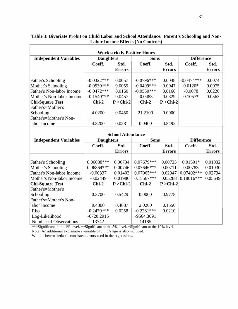
Table 3 presents the results from regressing the child labor indicator variables on
the father’s and mother’s schooling and non-labor income. First, note that the
coefficients of parent’s schooling do not change markedly between Tables 2 and 3.
Again, a father’s schooling has a stronger negative impact on a son’s child labor status
than a daughter’s, a mother’s schooling has a stronger negative effect on a daughter’s
child labor status than a son’s, and both a mother’s and a father’s schooling has a stronger
impact (although not significant for mothers) on a son’s school attendance than a
daughter’s. Second, note that similar results hold for the parents’ non-labor income. A
mother’s non-labor income has a stronger negative impact on a daughter’s child labor
status compared to a father’s non-labor income. On the other hand, a father’s non-labor
income seems to have a greater impact on a son’s child labor status compared to a
mother’s, although statistically they are not significantly different.
As in Table 2, the results given in Table 3 show that fathers have a greater impact
on sons and mothers have a greater impact on daughters concerning the decision to send a
child to the labor market. Regarding school attendance, an interesting pattern emerges.
A father’s non-labor income and a mother’s non-labor income do not affect a daughter’s
school attendance status, but they do affect a son’s likelihood of attending school, and
these differences are statistically significant, as shown in the last two columns of the
panel in the bottom of Table 3.
11 One must be cautious in attributing the difference in outcomes to technology. For example, a motherwith non-labor income who spends it on a maid may create a household environment that demand lesswork of daughters and therefore creates a more conducive learning environment leading to a higher humancapital return on her education. But this is precisely a result of the mother asserting her preferences, not adifference in the human capital technology that arises out of the mother’s non-labor income.

17
The results of Tables 2 and 3 clearly show that fathers and mothers have different
impacts on a child’s probability of working in the labor market. Parental education and
resources have different effects across a child’s likelihood of being a child laborer.
However, both fathers and mothers seem to impact sons greater than daughters regarding
school attendance. Although each parent’s schooling coefficients do not differ greatly
within and across siblings, their non-labor incomes are diverted preferentially to sons.
These results could be driven by intra-household bargaining or by the idiosyncratic
human capital technology. In order to attempt to isolate the effects of bargaining, we
next look at the difference in education levels of the parents, specifically, if the mother is
better educated than the father.
If schooling is associated with bargaining power in intra-household allocation
decisions, then mothers who are better educated than fathers should be more able to
impose their preferences. In order to discover if this is happening in our data, we
construct an indicator variable that equals one if the child is from a household where the
mother is more educated than the father. However, this indicator variable can also
capture the effect of non-linearities in the returns to schooling. In order to control for this
possibility, we add indicator variables for different levels of schooling for fathers and
mothers, separately. We divided their schooling attainment into five categories (illiterate,
0 to 4 years of schooling, 5 to 8 years of schooling, 9 to 11 years of schooling, and 12 or
more years of schooling). Therefore, a mother is considered to be more educated than a
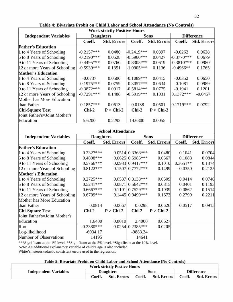
father if she belongs to a higher education category than the father. Tables 4 and 5
present the results of estimates of the same two bivariate probit modes from tables 2 and
3 but with the new indicator variables for education levels as well as the mother more
educated than the father variable.
18
Table 4 presents the results of the estimation without non-labor income, where
illiterate is the omitted variable and the only control variable is the child’s age. The
results show that, controlling for education, a daughter is less likely to work in the labor
market if her mother is more educated than her father. However, this result does not hold
for sons. The last row of each panel show the chi-square test of the joint schooling
effects where the null hypothesis is that this effect is equal between mothers and fathers.
We cannot reject the null hypothesis for daughters but do reject it for sons. As seen in
the last two columns, a father’s schooling has a stronger negative effect on a son’s
probability of working in the labor market compared to a daughter’s, for all education
levels. However, a mother’s schooling effect becomes stronger (although not
statistically significant) on a daughter’s likelihood of working in the labor market
compared to son’s only when her education level reaches 12 or more years of schooling.
Regarding school attendance, both a father’s and a mother’s schooling seem to be more
strongly associated with a son’s probability of going to school than a daughter’s.
Interestingly, a household where the mother is more educated than the father does not
effect a daughter’s nor a son’s probability of going to school.
Table 5 estimated the same model but with the parents’ non-labor income variable
included. The results are qualitatively the same as in previous tables. Most importantly,
a daughter from a household where the mother is more educated than the father is less
likely to work in the labor market, but there is no effect on a son’s probability of working
in the labor market. However, this has no effect on a daughter’s or a son’s probability of
going to school. These results support our previous findings that mothers favor daughters
and fathers favor sons regarding child labor decisions but both parents favor sons
regarding school attendance decisions.
19
Some caveats are worth mentioning at this point. As long as each spouse has
control over his or her own resources, these results can be explained by differences in the
human capital technology and/or differences in parent’s preferences as suggested by the
model above. However, the father’s schooling and mother’s schooling variables (or even
the non-labor income variables) may just be picking up other forces that affect child labor
and school attendance and, if so, we may be guilty of overstating our findings. In fact,
results from Emerson and Portela (2000) show that the child labor status of the parents is
an important element in explaining the child labor status of a son or a daughter. Also, it
shows that being a child laborer undermines the ability to generate labor earnings as an
adult. Thus, it would be natural to extend the empirical model to include parental child
labor status or the age they started to work. This can be interpreted as an additional
proxy for parental human capital, although it can also capture some sort of social norm
associated with child labor. Furthermore, empirical research on child labor (e.g, Grottaert
and Patrinos, 1999) has emphasized the role of family composition and community
characteristics on the determinants of child labor and schooling investment.
In order to account for these factors, we estimate a series of bivariate probit
models that include a vector of household characteristics: the age of the child, age of the
father and mother, the number of male siblings aged 0 to 5, 6 to 9, 10 to 14 and 15 to 17,
the number of female siblings aged 0 to 5, 6 to 9, 10 to 14 and 15 to 17 and an indicator
variable that equals one if the child lives in an urban area. In order to capture the effect
of parental child labor, we include the father’s age at which he started to work, and the
mother’s age at which she started to work. Since this information is obtained for those in
the labor market only and is missing for the others, we include indicator variables if the
father is either unemployed or not in the labor market and if the mother is either
20
unemployed or not in the labor market. Although the unemployment or not in the labor
market status of the parents variables are potentially endogenous, they are important to
control for potential bias derived from the missing information on the age started to work.
In fact, most of these control variables are potentially endogenous to some degree, so
these regressions may not be giving us a more accurate estimate of the effects of
schooling and non-labor income. However, these results are useful in that they provide
information about the degree to which the schooling and non-labor income coefficients
are capturing the effects of other variables correlated with child labor and child’s
schooling.12
Because the results of the estimations given in tables 2 and 3 are qualitatively yhe
same as in tables 4 and 5 we estimate only the models from tables 2 and 3 with these
controls. The results of these estimations are given in tables 6 and 7. In Table 6, note
that the estimates of father’s schooling and mother’s schooling on child labor and school
attendance decisions are smaller now but the results are qualitatively similar to those
given in Table 2. Second, the older the father was when he started to work, the less likely
to be a laborer is his child, and this impact is stronger on sons than on daughters.
Conversely, the older the mother was when she started to work, the less likely to work
her child is, and this effect is stronger on daughters than on sons. Third, the father’s age
started to work and mother’s age started to work variables do not affect a child’s
probability of going to school.
Table 7 presents the results of an estimation of the same model as in Table 6, but
with fathers’ non-labor income and mothers’ non-labor income included. The results in
12 Another important caveat is the potential endogeneity of the non-labor income variables. However, dueto the lack of adequate instruments, we opted to present regression results with and without non-laborincome variables.
21
Table 7 are qualitatively the same for all the previous variables used in Table 6.
Moreover, a mother’s non-labor income has a negative impact on a daughter’s child labor
status, and both a mother’s and a father’s non-labor income has a positive impact on a
son’s school attendance. Similar to the results of Table 3, where no controls were added,
this difference of parental non-labor income on children’s school attendance is
significantly greater for sons than for daughters. The robustness of this result bolsters our
confidence in saying that both fathers and mothers have a greater impact on the education
of sons in the household than on the education of daughters.
Why do parents favor sons in schooling investment? It is possible that the returns
to education for sons are generally higher than for daughters and so parents, who care
about the human capital of all children, will direct resources to the children with the
highest marginal returns. Alternatively, it may be that the opportunity cost of schooling
is higher for daughters than for sons due to, for instance, household activities normatively
performed by females. Indeed, from Table 1 we can see that 6.6 percent of daughters and
8.3 percent of sons don't attend school. However, among those that don't attend school,
more than 76 percent of daughters don't work in the labor market either, in contrast with
56 percent of sons. Thus, a daughter is more likely both not to attend school and not to
work in the labor market. Finally, it could be that in many families it is the role of the
male children to take care of the parents when they are old. If this is so, both parents may
prefer to ensure that their sons have high human capital in relation to their daughters,
whose human capital returns may soon be lost to another family through marriage.
To provide a test of the robustness of the results in Tables 6 and 7, we estimate
the same bivariate probit models but replace the parents’ age started to work with an
indicator variable that equals one if the father (mother) started to work at age fourteen or
22
below. We also estimate models where we replace the children’s child labor indicator
variable that equals one if they usually work any strictly positive hours with an indicator
variable that equals one only if they usually work at least 20 hours per week.
Furthermore, we estimate models using the over 20 hours per week definition of
children’s child labor with the parental child labor indicator variable, as well as
estimating the same models but as probit models on children’s child labor and school
attendance separately. These estimations give essentially the same results and are
presented in the Appendix.
V. Conclusion
This paper investigates intra-household gender differences and the incidence of
child labor and children’s school attendance in Brazil. The main results can be
summarized as follows:
First, higher parental education increases the probability that a child will attend
school and decreases the likelihood of a child becoming a child laborer. However, these
impacts differ across sons and daughters. A father's schooling impacts a son's child labor
and school attendance more than a daughter's. A mother's schooling has stronger impact
on a daughter's child labor status than on a son's, and impacts a son's and a daughter's
school attendance either equally or slightly stronger for a son's. In addition, in
households where the mother has more education than the father, daughters are more
likely to be withheld from the labor market.
Second, a father’s and a mother's non-labor income has no impact at all on a
daughter's school attendance but a positive and significant impact on a son's school
attendance. A father's non-labor income does not affect the children’s child labor status
23
but a mother's non-labor income decreases the likelihood of a daughter being a child
laborer.
Third, as found in Emerson and Portela (2000), there is a strong inter-generational
persistence of child labor. Moreover, the results suggest that a father having been a child
laborer impacts a son's child labor and school attendance more than a daughter’s. On the
other hand, a mother having been a child laborer seems to impact sons and daughters
equally in school attendance, and may impact daughters slightly more in child labor
status.
These results together suggest that both parents seem to direct more resources
toward a son’s education than to a daughter’s education. On the other hand, they seem to
have separate and distinct impacts on the child labor incidence of their children,
depending on gender. Fathers have greater mitigating impact on sons and mothers have a
greater mitigating impact on daughters when it comes to the children working in the labor
market. These results could be evidence in support of Basu’s (2001) hypothesis that
spouses bargain over some dimensions in the intra-household allocations but not over
others. If parental education and non-labor income reflect, at least in part, bargaining
power in household allocation decisions, our results suggest that gender differences in
resource allocation could be related to differences in parental preferences as well as
differences in human capital technology. This suggests that it may be worthwhile to
consider richer models of household decision making in the child labor context.
A possible family arrangement consistent with these findings is that parents
anticipate relative higher returns to male education and at the same time assign household
work activities to daughters due to, e.g., social norms. Thus, a daughter’s lower relative
returns from education and the relatively higher opportunity cost of sending her to school
24
lead the parents to favor a son’s educational attainment over a daughter’s. When it comes
to the decision to remove a child from the labor market, fathers prefer to remove the son
because he may value more the returns to education and mothers prefer to remove the
daughter because she may value more the daughter's time at home.
Whatever the arrangement may be, the results have potentially important policy
implications. It may be that policies designed to ban child labor and increase schooling
attendance should take into account the child's gender in a family context. For example,
some programs aimed to reduce child labor assign transfers to families that keep their
children out of work and at school. The findings of this paper suggest that these
programs may need to consider not only the recipient of the transfer - the mother or the
father - but also the gender of the ultimate beneficiary - the son or the daughter. It is
clear that the opportunity cost of being at school is not only the forgone wage but also the
forgone value of doing other activities beyond working in the labor market and the
transfer scheme may account for this, particularly if the goal is to increase females
educational attainment.

25
Appendix
In this appendix we present descriptive statistics of the data employed in this
study as well as results from a series of related regressions.
The un-weighted means of all the variables used in the empirical analysis of this
paper are given in Table A.1. The results from the estimated models using parents’ child
labor indicator variables are given in Tables A.2 and A.3. The results from the
estimations using the over 20 hours in the sample week definition of children’s child
labor with the parental age started to work are given in Tables A.4 and A.5, and with
parents’ child labor indicator variables are given in Tables A.6 and A.7. The results from
estimating the same specifications but as probit models on children’s child labor and
school attendance separately are given in Tables A.8 and A.9, respectively.
26
References
Baland, Jean-Marie, and James A. Robinson. (2000) “Is Child Labor Inefficient?,”
Journal of Political Economy, 108:4, pp. 663-679.
Basu, Kaushik. (2001) “Gender and Say: A Model of Household Behavior with
Endogenously-determined Balance of Power,” Cornell University, mimeo.
__________. (1999) “Child Labor: Cause, Consequence, and Cure,” Journal of
Economic Literature, 37:3, pp.1083-1119.
Basu, Kaushik, and Pham Hoang Van. (1998) “The Economics of Child Labor,”
American Economic Review, 88:3, pp. 412-427.
Becker, Gary. (1982) Treatise on the Family. (Cambridge, MA: Harvard University
Press).
Behrman, Jere. (1997) “Intra-household Distribution and The family,” In: M.K.
Rosenzweig and O. Stark (eds.), Handbook of Population and Family Economics,
vol. 1A, Amsterdam: North-Holland.
___________. (1988) “Intra-household Allocation of Nutrients in Rural India: Are Boys
Favored? Do Parents Exhibit Inequality Aversion?,” Oxford Economic Papers,
40: 32-54.
Bell, Clive, and Hans Gersbach. (2000) “Child Labor and the Education of a Society,”
mimeo.
Browninig, M. and P.A. Chiappori (1998) “Efficient Intra-Household Allocations: A
General Characterization and Empirical Tests,” Econometrica, 66: 1241-1278.
Chiappori, Pierre-André. (1992) “Collective Labor Supply and Welfare,” Journal of
Political Economy, 100: 437-467.
27
__________. (1988) “Rational Household Labor Supply,” Econometrica, 56: 63-89.
Dessy, Sylvain. (2000) “A defense of Compulsory Measures Against Child Labor,”
Journal of Development Economics, 62: 261-275.
Emerson, Patrick and André Portela. (2000) “Is There a Child Labor Trap? Inter-
Generational Persistence of Child labor in Brazil,” Cornell University Department
of Economics Working Paper no. 471.
Glomm, Gerhard. (1997) “Parental Choice of Human Capital Investment,” Journal of
Development Economics, 53:1, pp. 99-114.
Grootaert, Christiaan, and Harry Anthony Patrinos, eds. (1999) Policy Analysis of Child
Labor: A Comparative Study. New York: St. Martin’s Press.
Jensen, Peter, and Helena Skyt Neilsen. (1997) “Child Labour or School Attendance?
Evidence from Zambia,” Journal of Population Economics, 10:4, pp. 407-424.
Lundberg, S. and R.A. Pollack. (1993) “Separate Spheres Bargaining and The Marriage
Market,” Journal of Political Economy, 6: 988-1010.
McElroy, M. (1990) “The Empirical Content of Nash-Bargained Household Behavior,”
Journal of Human Resources, 25: 559-583.
McElroy, M. and M. Horney. (1981) “Nash-Bargained Household Decisions: Toward a
Generalization of The Theory of Demand,” International Economic Review, 22:
333-349.
Ray, Ranjan. (2000) “Analysis of Child Labour in Peru and Pakistan: A Comparative
Study,” Journal of Population Economics, 13:1, pp. 3-19.
Ridao-Cano, Cristobal. (2000) “Child Labor and Schooling in a Low Income Rural
Economy,” University of Colorado, mimeo.
28
Sen, Amartya. (1990) “More Than 100 Million Women Missing,” New York Review of
Books, v. 37, pp. 61-66.
__________. (1984) “Family and Food: Sex Bias in Poverty,” In: A. Sen (eds.),
Resources, Value and Development. London: Blackwell.
Strauss, J. and D. Thomas. (1990) “Human Resources: Empirical Modeling of
Household and family Decisions,” in: J.R. Behrman and T.N. Srinivasan (eds.)
Handbook of Development Economics, vol. 3, Amsterdam: North Holland.
Tiefenthaler, Jill. (1999) “The Sectoral Labor Supply of Married Couples in Brazil:
Testing The Unitary Model of Household Behavior,” Journal of Population
Economics, 12: 591-606.
Thomas, Duncan. (1994) “Like father, Like Son; Like Mother, Like Daughter: Parental
resources and Child Height,” Journal of Human Resources, 29: 950-989.
__________. (1990) “Intra-household Resource Allocation: An Inferential Approach,”
Journal of Human Resources, 25: 635-664.
29
Table 1: Child Labor and School AttendanceSchool Attendance
Sons DaughtersChild Labor No Yes Total No Yes TotalNo Number 678 11174 11852 719 12249 12968
Row % 5.72 94.28 100 5.54 94.46 100Column% 56.08 83.19 80.95 76.49 92.41 91.36
Yes Number 531 2258 2789 221 1006 1227Row % 19.04 80.96 100 18.01 81.99 100Column% 43.92 16.81 19.05 23.51 7.59 8.64
Total Number 1209 13432 14641 940 13255 14195Row % 8.26 91.74 100 6.62 93.38 100Column% 100 100 100 100 100 100
30
Table 2: Bivariate Probit on Child Labor and School Attendance. Parent’s SchoolingEffects (No Controls)
Work strictly Positive HoursDaughters Sons DifferenceIndependent Variables
Coeff. Std.Errors
Coeff. Std.Errors
Coeff. Std.Errors
Father’s Schooling -0.0350*** 0.0056 -0.0824*** 0.0047 -0.0474*** 0.0073
Mother’s Schooling -0.0535*** 0.0057 -0.0436*** 0.0046 0.0099 0.0073
Chi-Square Test Chi-2 P >Chi-2 Chi-2 P >Chi-2
Father's=Mother's Schooling 3.3900 0.0066 22.1900 0.0000
School AttendanceDaughters Sons DifferenceIndependent Variables
Coeff. Std.Errors
Coeff. Std.Errors
Coeff. Std.Errors
Father's Schooling 0.0606*** 0.0072 0.0784*** 0.0071 0.01779* 0.01012
Mother's Schooling 0.0668*** 0.0074 0.0779*** 0.0070 0.01103 0.01021
Chi-Square Test Chi-2 P >Chi-2 Chi-2 P >Chi-2Father's=Mother's Schooling
0.2500 0.6200 0.0000 0.9634Rho -0.2375*** 0.0255 -0.2318*** 0.0206Log-Likelihood -6925.25 -9840.03Number of Observations 14131 14565***Significant at the 1% level. **Significant at the 5% level. *Significant at the 10% level.Note: An additional explanatory variable of child’s age is also included.White’s heteroskedastic consistent errors used in the regressions.
31
Table 3: Bivariate Probit on Child Labor and School Attendance. Parent’s Schooling and Non-Labor Income Effects (No Controls)
Work strictly Positive HoursDaughters Sons DifferenceIndependent Variables
Coeff. Std.Errors
Coeff. Std.Errors
Coeff. Std.Errors
Father's Schooling -0.0322*** 0.0057 -0.0796*** 0.0048 -0.0474*** 0.0074Mother's Schooling -0.0530*** 0.0059 -0.0409*** 0.0047 0.0120* 0.0075Father's Non-labor Income -0.0472*** 0.0160 -0.0550*** 0.0160 -0.0078 0.0226Mother's Non-labor Income -0.1540*** 0.0457 -0.0483 0.0329 0.1057* 0.0563Chi-Square Test Chi-2 P >Chi-2 Chi-2 P >Chi-2Father's=Mother'sSchooling 4.0200 0.0450 21.2100 0.0000Father's=Mother's Non-labor Income 4.8200 0.0281 0.0400 0.8492
School AttendanceDaughters Sons DifferenceIndependent Variables
Coeff. Std.Errors
Coeff. Std.Errors
Coeff. Std.Errors
Father's Schooling 0.06088*** 0.00734 0.07679*** 0.00725 0.01591* 0.01032Mother's Schooling 0.06864*** 0.00746 0.07646*** 0.00711 0.00783 0.01030Father's Non-labor Income -0.00337 0.01403 0.07065*** 0.02347 0.07402*** 0.02734Mother's Non-labor Income -0.02449 0.01986 0.15567*** 0.05288 0.18016*** 0.05649Chi-Square Test Chi-2 P >Chi-2 Chi-2 P >Chi-2Father's=Mother'sSchooling 0.3700 0.5429 0.0000 0.9778Father's=Mother's Non-labor Income 0.4800 0.4887 2.0200 0.1550Rho -0.2470*** 0.0258 -0.2281*** 0.0210Log-Likelihood -6720.2915 -9564.3091Number of Observations 13742 14185***Significant at the 1% level. **Significant at the 5% level. *Significant at the 10% level.Note: An additional explanatory variable of child’s age is also included.White’s heteroskedastic consistent errors used in the regressions.
32
Table 5: Bivariate Probit on Child Labor and School Attendance (No Controls)Work strictly Postive Hours
Independent Variables Daughters Sons DifferenceCoeff. Std. Errors Coeff. Std. Errors Coeff. Std. Errors
Table 4: Bivariate Probit on Child Labor and School Attendance (No Controls)Work strictly Positive Hours
Independent Variables Daughters Sons DifferenceCoeff. Std. Errors Coeff. Std. Errors Coeff. Std. Errors
Father's Education1 to 4 Years of Schooling -0.2157*** 0.0486 -0.2419*** 0.0397 -0.0262 0.06285 to 8 Years of Schooling -0.2190*** 0.0528 -0.5960*** 0.0427 -0.3770*** 0.06799 to 11 Years of Schooling -0.4495*** 0.0760 -0.8305*** 0.0619 -0.3810*** 0.098012 or more Years of Schooling -0.5939*** 0.1351 -1.0905*** 0.1136 -0.4966** 0.1765Mother's Education1 to 4 Years of Schooling -0.0737 0.0500 -0.1089*** 0.0415 -0.0352 0.06505 to 8 Years of Schooling -0.1975*** 0.0759 -0.3057*** 0.0634 -0.1081 0.09899 to 11 Years of Schooling -0.3872*** 0.0917 -0.5814*** 0.0775 -0.1941 0.120112 or more Years of Schooling -0.7291*** 0.1488 -0.5919*** 0.1031 0.1372*** -0.0457Mother has More Educationthan Father -0.1857*** 0.0613 -0.0138 0.0501 0.1719*** 0.0792Chi-Square Test Chi-2 P > Chi-2 Chi-2 P > Chi-2Joint Father's=Joint Mother'sEducation 5.6200 0.2292 14.6300 0.0055
School AttendanceIndependent Variables Daughters Sons Difference
Coeff. Std. Errors Coeff. Std. Errors Coeff. Std. ErrorsFather's Education1 to 4 Years of Schooling 0.2327*** 0.0514 0.3368*** 0.0480 0.1041 0.07045 to 8 Years of Schooling 0.4898*** 0.0625 0.5985*** 0.0567 0.1088 0.08449 to 11 Years of Schooling 0.5766*** 0.0933 0.9417*** 0.1010 0.3651** 0.137412 or more Years of Schooling 0.8122*** 0.1507 0.7772*** 0.1499 -0.0350 0.2125Mother's Education1 to 4 Years of Schooling 0.2725*** 0.0537 0.3138*** 0.0509 0.0414 0.07405 to 8 Years of Schooling 0.5241*** 0.0871 0.5642*** 0.0815 0.0401 0.11939 to 11 Years of Schooling 0.6667*** 0.1101 0.7529*** 0.1039 0.0862 0.151412 or more Years of Schooling 0.6709*** 0.1445 0.9499*** 0.1673 0.2790 0.2211Mother has More Educationthan Father 0.0814 0.0667 0.0298 0.0626 -0.0517 0.0915Chi-Square Test Chi-2 P > Chi-2 Chi-2 P > Chi-2Joint Father's=Joint Mother'sEducation 1.6400 0.8010 2.4000 0.6627 Rho -0.2380*** 0.0254-0.2385*** 0.0205Log-likelihood -6934.17 -9883.34Number of Observations 14195 14641 ***Significant at the 1% level. **Significant at the 5% level. *Significant at the 10% level.Note: An additional explanatory variable of child’s age is also included.White’s heteroskedastic consistent errors used in the regression.
33
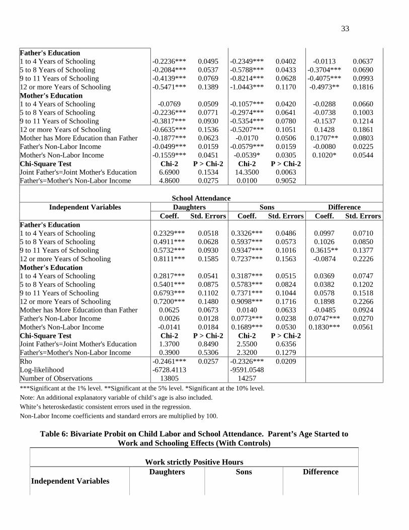
Father's Education1 to 4 Years of Schooling -0.2236*** 0.0495 -0.2349*** 0.0402 -0.0113 0.06375 to 8 Years of Schooling -0.2084*** 0.0537 -0.5788*** 0.0433 -0.3704*** 0.06909 to 11 Years of Schooling -0.4139*** 0.0769 -0.8214*** 0.0628 -0.4075*** 0.099312 or more Years of Schooling -0.5471*** 0.1389 -1.0443*** 0.1170 -0.4973** 0.1816Mother's Education1 to 4 Years of Schooling -0.0769 0.0509 -0.1057*** 0.0420 -0.0288 0.06605 to 8 Years of Schooling -0.2236*** 0.0771 -0.2974*** 0.0641 -0.0738 0.10039 to 11 Years of Schooling -0.3817*** 0.0930 -0.5354*** 0.0780 -0.1537 0.121412 or more Years of Schooling -0.6635*** 0.1536 -0.5207*** 0.1051 0.1428 0.1861Mother has More Education than Father -0.1877*** 0.0623 -0.0170 0.0506 0.1707** 0.0803Father's Non-Labor Income -0.0499*** 0.0159 -0.0579*** 0.0159 -0.0080 0.0225Mother's Non-Labor Income -0.1559*** 0.0451 -0.0539* 0.0305 0.1020* 0.0544Chi-Square Test Chi-2 P > Chi-2 Chi-2 P > Chi-2Joint Father's=Joint Mother's Education 6.6900 0.1534 14.3500 0.0063Father's=Mother's Non-Labor Income 4.8600 0.0275 0.0100 0.9052
School AttendanceIndependent Variables Daughters Sons Difference
Coeff. Std. Errors Coeff. Std. Errors Coeff. Std. ErrorsFather's Education1 to 4 Years of Schooling 0.2329*** 0.0518 0.3326*** 0.0486 0.0997 0.07105 to 8 Years of Schooling 0.4911*** 0.0628 0.5937*** 0.0573 0.1026 0.08509 to 11 Years of Schooling 0.5732*** 0.0930 0.9347*** 0.1016 0.3615** 0.137712 or more Years of Schooling 0.8111*** 0.1585 0.7237*** 0.1563 -0.0874 0.2226Mother's Education1 to 4 Years of Schooling 0.2817*** 0.0541 0.3187*** 0.0515 0.0369 0.07475 to 8 Years of Schooling 0.5401*** 0.0875 0.5783*** 0.0824 0.0382 0.12029 to 11 Years of Schooling 0.6793*** 0.1102 0.7371*** 0.1044 0.0578 0.151812 or more Years of Schooling 0.7200*** 0.1480 0.9098*** 0.1716 0.1898 0.2266Mother has More Education than Father 0.0625 0.0673 0.0140 0.0633 -0.0485 0.0924Father's Non-Labor Income 0.0026 0.0128 0.0773*** 0.0238 0.0747*** 0.0270Mother's Non-Labor Income -0.0141 0.0184 0.1689*** 0.0530 0.1830*** 0.0561Chi-Square Test Chi-2 P > Chi-2 Chi-2 P > Chi-2Joint Father's=Joint Mother's Education 1.3700 0.8490 2.5500 0.6356Father's=Mother's Non-Labor Income 0.3900 0.5306 2.3200 0.1279Rho -0.2461*** 0.0257 -0.2326*** 0.0209Log-likelihood -6728.4113 -9591.0548Number of Observations 13805 14257***Significant at the 1% level. **Significant at the 5% level. *Significant at the 10% level.
Note: An additional explanatory variable of child’s age is also included.
White’s heteroskedastic consistent errors used in the regression.
Non-Labor Income coefficients and standard errors are multiplied by 100.
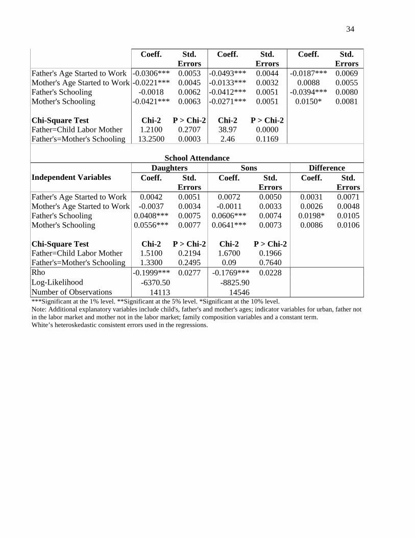
Table 6: Bivariate Probit on Child Labor and School Attendance. Parent’s Age Started toWork and Schooling Effects (With Controls)
Work strictly Positive Hours
Independent VariablesDaughters Sons Difference
34
Coeff. Std.Errors
Coeff. Std.Errors
Coeff. Std.Errors
Father's Age Started to Work -0.0306*** 0.0053 -0.0493*** 0.0044 -0.0187*** 0.0069Mother's Age Started to Work -0.0221*** 0.0045 -0.0133*** 0.0032 0.0088 0.0055Father's Schooling -0.0018 0.0062 -0.0412*** 0.0051 -0.0394*** 0.0080Mother's Schooling -0.0421*** 0.0063 -0.0271*** 0.0051 0.0150* 0.0081
Chi-Square Test Chi-2 P > Chi-2 Chi-2 P > Chi-2Father=Child Labor Mother 1.2100 0.2707 38.97 0.0000Father's=Mother's Schooling 13.2500 0.0003 2.46 0.1169
School AttendanceDaughters Sons Difference
Independent Variables Coeff. Std.Errors
Coeff. Std.Errors
Coeff. Std.Errors
Father's Age Started to Work 0.0042 0.0051 0.0072 0.0050 0.0031 0.0071Mother's Age Started to Work -0.0037 0.0034 -0.0011 0.0033 0.0026 0.0048Father's Schooling 0.0408*** 0.0075 0.0606*** 0.0074 0.0198* 0.0105Mother's Schooling 0.0556*** 0.0077 0.0641*** 0.0073 0.0086 0.0106
Chi-Square Test Chi-2 P > Chi-2 Chi-2 P > Chi-2Father=Child Labor Mother 1.5100 0.2194 1.6700 0.1966Father's=Mother's Schooling 1.3300 0.2495 0.09 0.7640Rho -0.1999*** 0.0277 -0.1769*** 0.0228Log-Likelihood -6370.50 -8825.90Number of Observations 14113 14546***Significant at the 1% level. **Significant at the 5% level. *Significant at the 10% level.Note: Additional explanatory variables include child's, father's and mother's ages; indicator variables for urban, father notin the labor market and mother not in the labor market; family composition variables and a constant term.White’s heteroskedastic consistent errors used in the regressions.

35
Table 7: Bivariate Probit on Child Labor and School Attendance. Parent’s AgeStarted to Work, Schooling and Non-Labor Income Effects (With Controls)
Work strictly Positive HoursDaughters Sons Difference
Independent Variables Coeff. Std.Errors
Coeff. Std.Errors
Coeff. Std. Errors
Father's Age Started to Work -0.0298*** 0.0054 -0.0502*** 0.0045 -0.0204*** 0.0070Mother's Age Started to Work -0.0218*** 0.0045 -0.0131*** 0.0032 0.0087 0.0055Father's Schooling -0.0010 0.0063 -0.0400*** 0.0052 -0.0390*** 0.0082Mother's Schooling -0.0418*** 0.0065 -0.0248* 0.0052 0.0170** 0.0083Father's Non-Labor Income -0.0054 0.0112 -0.0188 0.0117 -0.0134 0.0162Mother's Non-Labor Income -0.0642** 0.0317 -0.0208 0.0200 0.0434 0.0375Chi-Square Test Chi-2 P > Chi-2 Chi-2 P > Chi-2Father=Child Labor Mother 1.06 0.3034 39.8800 0.0000Father's=Mother's Schooling 13.21 0.0003 2.78 0.0955Father's=Mother's Non-LaborIncome
3.05 0.0809 0.01 0.9308
School AttendanceDaughters Sons Difference
Independent Variables Coeff. Std.Errors
Coeff. Std.Errors
Coeff. Std. Errors
Father's Age Started to Work 0.0055 0.0052 0.0094* 0.0051 0.0039 0.0073Mother's Age Started to Work -0.0031 0.0035 -0.0021 0.0034 0.0010 0.0048Father's Schooling 0.0406*** 0.0077 0.0575*** 0.0075 0.0169 0.0107Mother's Schooling 0.0567*** 0.0077 0.0605*** 0.0074 0.0038 0.0107Father's Non-Labor Income -0.0022 0.0136 0.0754*** 0.0275 0.0776** 0.0307Mother's Non-Labor Income -0.0255 0.0181 0.1747*** 0.0565 0.2002*** 0.0593Chi-Square Test Chi-2 P > Chi-2 Chi-2 P > Chi-2Father=Child Labor Mother 1.72 0.1897 3.05 0.0809Father's=Mother's Schooling 1.52 0.2170 0.06 0.8066Father's=Mother's Non-LaborIncome
0.66 0.4181 2.40 0.1210
Rho -0.2079*** 0.0279 -0.1794*** 0.0231Log-Likelihood -6200.48 -8601.60Number of Observations 13729 14171***Significant at the 1% level. **Significant at the 5% level. *Significant at the 10% level.Note: Additional explanatory variables include child's, father's and mother's ages; indicator variables for urban, father not in the labor marketand mother not in the labor market; family composition variables and a constant term.White’s heteroskedastic consistent errors used in the regressions.
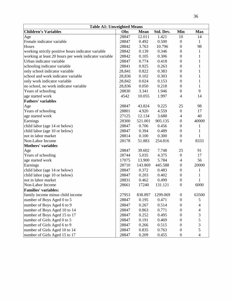
36
Table A1: Unweighted MeansChildren’s Variables Obs Mean Std. Dev. Min MaxAge 28847 12.011 1.421 10 14Female indicator variable 28847 0.492 0.500 0 1Hours 28842 3.763 10.796 0 98working strictly positive hours indicator variable 28842 0.139 0.346 0 1working at least 20 hours per week indicator variable 28842 0.105 0.306 0 1Urban indicator variable 28847 0.774 0.418 0 1schooling indicator variable 28841 0.925 0.263 0 1only school indicator variable 28,841 0.822 0.383 0 1school and work indicator variable 28,836 0.102 0.303 0 1only work indicator variable 28,842 0.024 0.153 0 1no school, no work indicator variable 28,836 0.050 0.218 0 1Years of schooling 28830 3.341 1.946 0 9age started work 4542 10.055 1.997 4 14Fathers' variablesAge 28847 43.824 9.225 25 98Years of schooling 28801 4.920 4.559 0 17age started work 27125 12.134 3.688 4 40Earnings 28300 521.001 905.135 0 40000child labor (age 14 or below) 28847 0.706 0.456 0 1child labor (age 10 or below) 28847 0.394 0.489 0 1not in labor market 28814 0.100 0.300 0 1Non-Labor Income 28178 51.883 254.816 0 8333Mothers' variablesAge 28847 39.602 7.748 25 91Years of schooling 28744 5.035 4.375 0 17age started work 17075 13.900 5.784 4 56Earnings 28710 143.869 445.588 0 20000child labor (age 14 or below) 28847 0.372 0.483 0 1child labor (age 10 or below) 28847 0.203 0.402 0 1not in labor market 28831 0.462 0.499 0 1Non-Labor Income 28661 17240 131.121 0 6000Families' variables:family income minus child income 27953 838.897 1299.069 0 63500number of Boys Aged 0 to 5 28847 0.195 0.471 0 5number of Boys Aged 6 to 9 28847 0.267 0.514 0 4number of Boys Aged 10 to 14 28847 0.863 0.771 0 4number of Boys Aged 15 to 17 28847 0.252 0.495 0 3number of Girls Aged 0 to 5 28847 0.191 0.469 0 5number of Girls Aged 6 to 9 28847 0.266 0.515 0 3number of Girls Aged 10 to 14 28847 0.835 0.763 0 5number of Girls Aged 15 to 17 28847 0.209 0.455 0 4
37
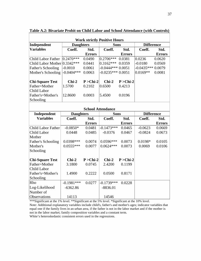
Table A.2: Bivariate Probit on Child Labor and School Attendance (with Controls)
Work strictly Positive HoursDaughters Sons DifferenceIndependent
Variables Coeff. Std.Errors
Coeff. Std.Errors
Coeff. Std.Errors
Child Labor Father 0.2470*** 0.0490 0.2706*** 0.0381 0.0236 0.0620Child Labor Mother 0.3342*** 0.0441 0.3162*** 0.0359 -0.0180 0.0569Father's Schooling -0.0010 0.0061 -0.0444*** 0.0051 -0.0435*** 0.0079Mother's Schooling -0.0404*** 0.0063 -0.0235*** 0.0051 0.0169** 0.0081
Chi-Square Test Chi-2 P >Chi-2 Chi-2 P >Chi-2Father=MotherChild Labor
1.5700 0.2102 0.6500 0.4213
Father's=Mother'sSchooling
12.8600 0.0003 5.4500 0.0196
School AttendanceDaughters Sons DifferenceIndependent
Variables Coeff. Std.Errors
Coeff. Std.Errors
Coeff. Std.Errors
Child Labor Father -0.0850* 0.0481 -0.1473*** 0.0465 -0.0623 0.0669Child LaborMother
0.0448 0.0485 -0.0376 0.0467 -0.0824 0.0673
Father's Schooling 0.0398*** 0.0074 0.0596*** 0.0073 0.0198* 0.0105Mother'sSchooling
0.0555*** 0.0077 0.0624*** 0.0073 0.0069 0.0106
Chi-Square Test Chi-2 P >Chi-2 Chi-2 P >Chi-2Father=MotherChild Labor
3.1800 0.0745 2.4200 0.1199
Father's=Mother'sSchooling
1.4900 0.2222 0.0500 0.8171
Rho -0.1981*** 0.0277 -0.1739*** 0.0228Log-Likelihood -6362.86 -8836.01Number ofObservations 14113 14546***Significant at the 1% level. **Significant at the 5% level. *Significant at the 10% level.Note: Additional explanatory variables include child's, father's and mother's ages; indicator variables thatequal one if the family lives in an urban area, if the father is not in the labor market and if the mother isnot in the labor market; family composition variables and a constant term.White’s heteroskedastic consistent errors used in the regressions.
38
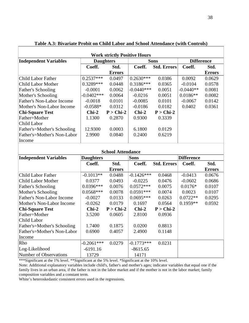
Table A.3: Bivariate Probit on Child Labor and School Attendance (with Controls)
Work strictly Positive HoursDaughters Sons DifferenceIndependent Variables
Coeff. Std.Errors
Coeff. Std. Errors Coeff. Std.Errors
Child Labor Father 0.2537*** 0.0497 0.2630*** 0.0386 0.0092 0.0629Child Labor Mother 0.3289*** 0.0448 0.3186*** 0.0365 -0.0104 0.0578Father's Schooling -0.0001 0.0062 -0.0440*** 0.0051 -0.0440** 0.0081Mother's Schooling -0.0402*** 0.0064 -0.0216 0.0051 0.0186** 0.0082Father's Non-Labor Income -0.0018 0.0101 -0.0085 0.0101 -0.0067 0.0142Mother's Non-Labor Income -0.0588* 0.0312 -0.0186 0.0182 0.0402 0.0361Chi-Square Test Chi-2 P > Chi-2 Chi-2 P > Chi-2Father=MotherChild Labor
1.1300 0.2870 0.9300 0.3339
Father's=Mother's Schooling 12.9300 0.0003 6.1800 0.0129Father's=Mother's Non-LaborIncome
2.9900 0.0840 0.2400 0.6219
School AttendanceDaughters Sons DifferenceIndependent Variables
Coeff. Std.Errors
Coeff. Std. Errors Coeff. Std.Errors
Child Labor Father -0.1013** 0.0488 -0.1426*** 0.0468 -0.0413 0.0676Child Labor Mother 0.0377 0.0493 -0.0225 0.0476 -0.0602 0.0686Father's Schooling 0.0396*** 0.0076 0.0572*** 0.0075 0.0176* 0.0107Mother's Schooling 0.0568*** 0.0078 0.0591*** 0.0074 0.0023 0.0107Father's Non-Labor Income -0.0027 0.0133 0.0695*** 0.0263 0.0722** 0.0295Mother's Non-Labor Income -0.0262 0.0179 0.1697 0.0564 0.1959** 0.0592Chi-Square Test Chi-2 P > Chi-2 Chi-2 P > Chi-2Father=MotherChild Labor
3.5200 0.0605 2.8100 0.0936
Father's=Mother's Schooling 1.7400 0.1875 0.0200 0.8813Father's=Mother's Non-LaborIncome
0.6900 0.4057 2.4900 0.1148
Rho -0.2061*** 0.0279 -0.1773*** 0.0231Log-Likelihood -6191.16 -8615.65Number of Observations 13729 14171***Significant at the 1% level. **Significant at the 5% level. *Significant at the 10% level.Note: Additional explanatory variables include child's, father's and mother's ages; indicator variables that equal one if thefamily lives in an urban area, if the father is not in the labor market and if the mother is not in the labor market; familycomposition variables and a constant term.White’s heteroskedastic consistent errors used in the regressions.
39
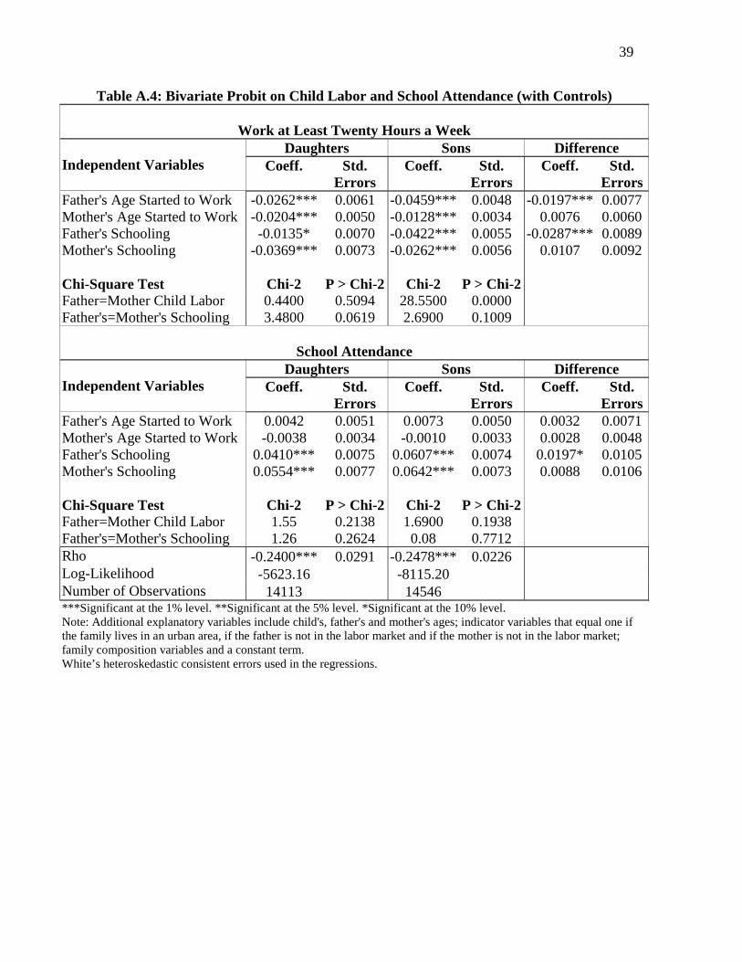
Table A.4: Bivariate Probit on Child Labor and School Attendance (with Controls)
Work at Least Twenty Hours a WeekDaughters Sons Difference
Independent Variables Coeff. Std.Errors
Coeff. Std.Errors
Coeff. Std.Errors
Father's Age Started to Work -0.0262*** 0.0061 -0.0459*** 0.0048 -0.0197*** 0.0077Mother's Age Started to Work -0.0204*** 0.0050 -0.0128*** 0.0034 0.0076 0.0060Father's Schooling -0.0135* 0.0070 -0.0422*** 0.0055 -0.0287*** 0.0089Mother's Schooling -0.0369*** 0.0073 -0.0262*** 0.0056 0.0107 0.0092
Chi-Square Test Chi-2 P > Chi-2 Chi-2 P > Chi-2Father=Mother Child Labor 0.4400 0.5094 28.5500 0.0000Father's=Mother's Schooling 3.4800 0.0619 2.6900 0.1009
School AttendanceDaughters Sons Difference
Independent Variables Coeff. Std.Errors
Coeff. Std.Errors
Coeff. Std.Errors
Father's Age Started to Work 0.0042 0.0051 0.0073 0.0050 0.0032 0.0071Mother's Age Started to Work -0.0038 0.0034 -0.0010 0.0033 0.0028 0.0048Father's Schooling 0.0410*** 0.0075 0.0607*** 0.0074 0.0197* 0.0105Mother's Schooling 0.0554*** 0.0077 0.0642*** 0.0073 0.0088 0.0106
Chi-Square Test Chi-2 P > Chi-2 Chi-2 P > Chi-2Father=Mother Child Labor 1.55 0.2138 1.6900 0.1938Father's=Mother's Schooling 1.26 0.2624 0.08 0.7712Rho -0.2400*** 0.0291 -0.2478*** 0.0226Log-Likelihood -5623.16 -8115.20Number of Observations 14113 14546***Significant at the 1% level. **Significant at the 5% level. *Significant at the 10% level.Note: Additional explanatory variables include child's, father's and mother's ages; indicator variables that equal one ifthe family lives in an urban area, if the father is not in the labor market and if the mother is not in the labor market;family composition variables and a constant term.White’s heteroskedastic consistent errors used in the regressions.
40
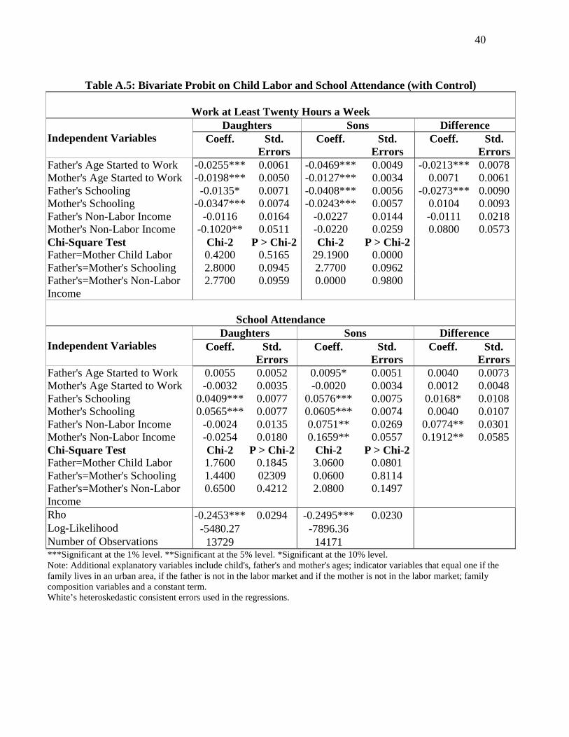
Table A.5: Bivariate Probit on Child Labor and School Attendance (with Control)
Work at Least Twenty Hours a WeekDaughters Sons Difference
Independent Variables Coeff. Std.Errors
Coeff. Std.Errors
Coeff. Std.Errors
Father's Age Started to Work -0.0255*** 0.0061 -0.0469*** 0.0049 -0.0213*** 0.0078Mother's Age Started to Work -0.0198*** 0.0050 -0.0127*** 0.0034 0.0071 0.0061Father's Schooling -0.0135* 0.0071 -0.0408*** 0.0056 -0.0273*** 0.0090Mother's Schooling -0.0347*** 0.0074 -0.0243*** 0.0057 0.0104 0.0093Father's Non-Labor Income -0.0116 0.0164 -0.0227 0.0144 -0.0111 0.0218Mother's Non-Labor Income -0.1020** 0.0511 -0.0220 0.0259 0.0800 0.0573Chi-Square Test Chi-2 P > Chi-2 Chi-2 P > Chi-2Father=Mother Child Labor 0.4200 0.5165 29.1900 0.0000Father's=Mother's Schooling 2.8000 0.0945 2.7700 0.0962Father's=Mother's Non-LaborIncome
2.7700 0.0959 0.0000 0.9800
School AttendanceDaughters Sons Difference
Independent Variables Coeff. Std.Errors
Coeff. Std.Errors
Coeff. Std.Errors
Father's Age Started to Work 0.0055 0.0052 0.0095* 0.0051 0.0040 0.0073Mother's Age Started to Work -0.0032 0.0035 -0.0020 0.0034 0.0012 0.0048Father's Schooling 0.0409*** 0.0077 0.0576*** 0.0075 0.0168* 0.0108Mother's Schooling 0.0565*** 0.0077 0.0605*** 0.0074 0.0040 0.0107Father's Non-Labor Income -0.0024 0.0135 0.0751** 0.0269 0.0774** 0.0301Mother's Non-Labor Income -0.0254 0.0180 0.1659** 0.0557 0.1912** 0.0585Chi-Square Test Chi-2 P > Chi-2 Chi-2 P > Chi-2Father=Mother Child Labor 1.7600 0.1845 3.0600 0.0801Father's=Mother's Schooling 1.4400 02309 0.0600 0.8114Father's=Mother's Non-LaborIncome
0.6500 0.4212 2.0800 0.1497
Rho -0.2453*** 0.0294 -0.2495*** 0.0230Log-Likelihood -5480.27 -7896.36Number of Observations 13729 14171***Significant at the 1% level. **Significant at the 5% level. *Significant at the 10% level.Note: Additional explanatory variables include child's, father's and mother's ages; indicator variables that equal one if thefamily lives in an urban area, if the father is not in the labor market and if the mother is not in the labor market; familycomposition variables and a constant term.White’s heteroskedastic consistent errors used in the regressions.
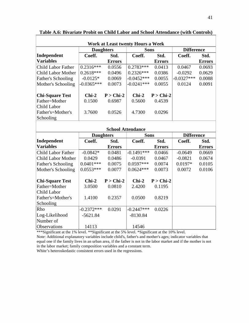
41
Table A.6: Bivariate Probit on Child Labor and School Attendance (with Controls)
Work at Least twenty Hours a WeekDaughters Sons Difference
IndependentVariables
Coeff. Std.Errors
Coeff. Std.Errors
Coeff. Std.Errors
Child Labor Father 0.2316*** 0.0556 0.2783*** 0.0413 0.0467 0.0693Child Labor Mother 0.2618*** 0.0496 0.2326*** 0.0386 -0.0292 0.0629Father's Schooling -0.0125* 0.0069 -0.0452*** 0.0055 -0.0327*** 0.0088Mother's Schooling -0.0365*** 0.0073 -0.0241*** 0.0055 0.0124 0.0091
Chi-Square Test Chi-2 P > Chi-2 Chi-2 P > Chi-2Father=MotherChild Labor
0.1500 0.6987 0.5600 0.4539
Father's=Mother'sSchooling
3.7600 0.0526 4.7300 0.0296
School AttendanceDaughters Sons Difference
IndependentVariables
Coeff. Std.Errors
Coeff. Std.Errors
Coeff. Std.Errors
Child Labor Father -0.0842* 0.0481 -0.1491*** 0.0466 -0.0649 0.0669Child Labor Mother 0.0429 0.0486 -0.0391 0.0467 -0.0821 0.0674Father's Schooling 0.0401*** 0.0075 0.0597*** 0.0074 0.0197* 0.0105Mother's Schooling 0.0553*** 0.0077 0.0624*** 0.0073 0.0072 0.0106
Chi-Square Test Chi-2 P > Chi-2 Chi-2 P > Chi-2Father=MotherChild Labor
3.0500 0.0810 2.4200 0.1195
Father's=Mother'sSchooling
1.4100 0.2357 0.0500 0.8219
Rho -0.2372*** 0.0291 -0.2447*** 0.0226Log-Likelihood -5621.84 -8130.84Number ofObservations 14113 14546***Significant at the 1% level. **Significant at the 5% level. *Significant at the 10% level.Note: Additional explanatory variables include child's, father's and mother's ages; indicator variables thatequal one if the family lives in an urban area, if the father is not in the labor market and if the mother is notin the labor market; family composition variables and a constant term.White’s heteroskedastic consistent errors used in the regressions.
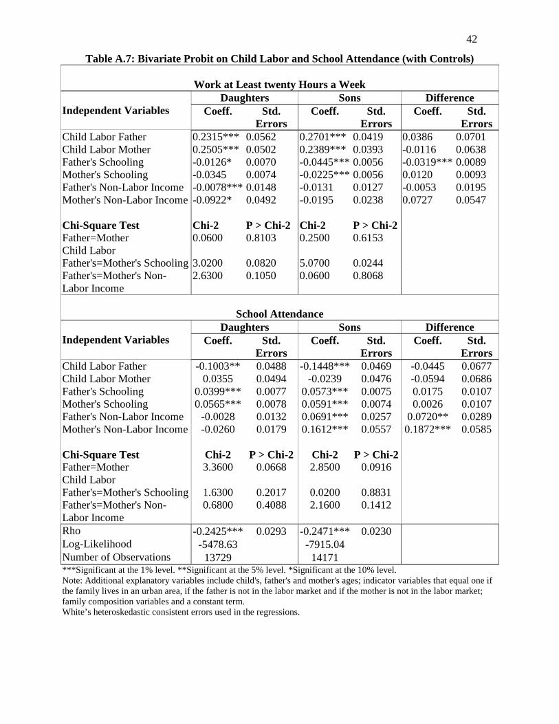
42
Table A.7: Bivariate Probit on Child Labor and School Attendance (with Controls)
Work at Least twenty Hours a WeekDaughters Sons Difference
Independent Variables Coeff. Std.Errors
Coeff. Std.Errors
Coeff. Std.Errors
Child Labor Father 0.2315*** 0.0562 0.2701*** 0.0419 0.0386 0.0701Child Labor Mother 0.2505*** 0.0502 0.2389*** 0.0393 -0.0116 0.0638Father's Schooling -0.0126* 0.0070 -0.0445*** 0.0056 -0.0319*** 0.0089Mother's Schooling -0.0345 0.0074 -0.0225*** 0.0056 0.0120 0.0093Father's Non-Labor Income -0.0078*** 0.0148 -0.0131 0.0127 -0.0053 0.0195Mother's Non-Labor Income -0.0922* 0.0492 -0.0195 0.0238 0.0727 0.0547
Chi-Square Test Chi-2 P > Chi-2 Chi-2 P > Chi-2Father=MotherChild Labor
0.0600 0.8103 0.2500 0.6153
Father's=Mother's Schooling 3.0200 0.0820 5.0700 0.0244Father's=Mother's Non-Labor Income
2.6300 0.1050 0.0600 0.8068
School AttendanceDaughters Sons Difference
Independent Variables Coeff. Std.Errors
Coeff. Std.Errors
Coeff. Std.Errors
Child Labor Father -0.1003** 0.0488 -0.1448*** 0.0469 -0.0445 0.0677Child Labor Mother 0.0355 0.0494 -0.0239 0.0476 -0.0594 0.0686Father's Schooling 0.0399*** 0.0077 0.0573*** 0.0075 0.0175 0.0107Mother's Schooling 0.0565*** 0.0078 0.0591*** 0.0074 0.0026 0.0107Father's Non-Labor Income -0.0028 0.0132 0.0691*** 0.0257 0.0720** 0.0289Mother's Non-Labor Income -0.0260 0.0179 0.1612*** 0.0557 0.1872*** 0.0585
Chi-Square Test Chi-2 P > Chi-2 Chi-2 P > Chi-2Father=MotherChild Labor
3.3600 0.0668 2.8500 0.0916
Father's=Mother's Schooling 1.6300 0.2017 0.0200 0.8831Father's=Mother's Non-Labor Income
0.6800 0.4088 2.1600 0.1412
Rho -0.2425*** 0.0293 -0.2471*** 0.0230Log-Likelihood -5478.63 -7915.04Number of Observations 13729 14171***Significant at the 1% level. **Significant at the 5% level. *Significant at the 10% level.Note: Additional explanatory variables include child's, father's and mother's ages; indicator variables that equal one ifthe family lives in an urban area, if the father is not in the labor market and if the mother is not in the labor market;family composition variables and a constant term.White’s heteroskedastic consistent errors used in the regressions.
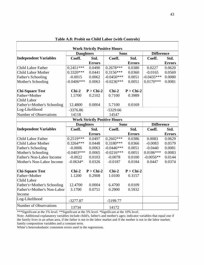
43
Table A.8: Probit on Child Labor (with Controls)
Work Strictly Positive HoursDaughters Sons Difference
Independent Variables Coeff. Std.Errors
Coeff. Std.Errors
Coeff. Std.Errors
Child Labor Father 0.2451*** 0.0490 0.2678*** 0.0380 0.0227 0.0620Child Labor Mother 0.3320*** 0.0441 0.3156*** 0.0360 -0.0165 0.0569Father's Schooling -0.0015 0.0062 -0.0450*** 0.0051 -0.0435*** 0.0080Mother's Schooling -0.0406*** 0.0063 -0.0236*** 0.0051 0.0170*** 0.0081
Chi-Square Test Chi-2 P > Chi-2 Chi-2 P > Chi-2Father=MotherChild Labor
1.5700 0.2102 0.7100 0.3989
Father's=Mother's Schooling 12.4800 0.0004 5.7100 0.0169Log-Likelihood -3376.86 -5329.66Number of Observations 14118 14547
Work Strictly Positive HoursDaughters Sons Difference
Independent Variables Coeff. Std.Errors
Coeff. Std.Errors
Coeff. Std.Errors
Child Labor Father 0.2519*** 0.0497 0.2602*** 0.0386 0.0083 0.0629Child Labor Mother 0.3264*** 0.0448 0.3180*** 0.0366 -0.0083 0.0579Father's Schooling -0.0006 0.0063 -0.0446*** 0.0051 -0.0440 0.0081Mother's Schooling -0.0403*** 0.0065 -0.0216*** 0.0051 0.0186*** 0.0083Father's Non-Labor Income -0.0022 0.0103 -0.0078 0.0100 -0.0056** 0.0144Mother's Non-Labor Income -0.0634* 0.0326 -0.0187 0.0184 0.0447 0.0374
Chi-Square Test Chi-2 P > Chi-2 Chi-2 P > Chi-2Father=MotherChild Labor
1.1200 0.2908 1.0100 0.3157
Father's=Mother's Schooling 12.4700 0.0004 6.4700 0.0109Father's=Mother's Non-LaborIncome
3.1700 0.0751 0.2900 0.5932
Log-Likelihood -3277.87 -5199.77Number of Observations 13734 14172***Significant at the 1% level. **Significant at the 5% level. *Significant at the 10% level.Note: Additional explanatory variables include child's, father's and mother's ages; indicator variables that equal one ifthe family lives in an urban area, if the father is not in the labor market and if the mother is not in the labor market;family composition variables and a constant term.White’s heteroskedastic consistent errors used in the regressions.
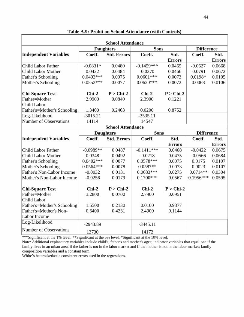
44
Table A.9: Probit on School Attendance (with Controls)
School AttendanceDaughters Sons Difference
Independent Variables Coeff. Std. Errors Coeff. Std.Errors
Coeff. Std.Errors
Child Labor Father -0.0831* 0.0480 -0.1459*** 0.0465 -0.0627 0.0668Child Labor Mother 0.0422 0.0484 -0.0370 0.0466 -0.0791 0.0672Father's Schooling 0.0403*** 0.0075 0.0601*** 0.0073 0.0198* 0.0105Mother's Schooling 0.0552*** 0.0077 0.0620*** 0.0072 0.0068 0.0106
Chi-Square Test Chi-2 P > Chi-2 Chi-2 P > Chi-2Father=MotherChild Labor
2.9900 0.0840 2.3900 0.1221
Father's=Mother's Schooling 1.3400 0.2463 0.0200 0.8752Log-Likelihood -3015.21 -3535.11Number of Observations 14114 14547
School AttendanceDaughters Sons Difference
Independent Variables Coeff. Std. Errors Coeff. Std.Errors
Coeff. Std.Errors
Child Labor Father -0.0989** 0.0487 -0.1411*** 0.0468 -0.0422 0.0675Child Labor Mother 0.0348 0.0492 -0.0218 0.0475 -0.0566 0.0684Father's Schooling 0.0402*** 0.0077 0.0578*** 0.0075 0.0175 0.0107Mother's Schooling 0.0564*** 0.0078 0.0587** 0.0073 0.0023 0.0107Father's Non-Labor Income -0.0032 0.0131 0.0683*** 0.0275 0.0714** 0.0304Mother's Non-Labor Income -0.0256 0.0179 0.1700*** 0.0567 0.1956*** 0.0595
Chi-Square Test Chi-2 P > Chi-2 Chi-2 P > Chi-2Father=MotherChild Labor
3.2800 0.0700 2.7900 0.0951
Father's=Mother's Schooling 1.5500 0.2130 0.0100 0.9377Father's=Mother's Non-Labor Income
0.6400 0.4231 2.4900 0.1144
Log-Likelihood -2943.89 -3445.11Number of Observations 13730 14172***Significant at the 1% level. **Significant at the 5% level. *Significant at the 10% level.Note: Additional explanatory variables include child's, father's and mother's ages; indicator variables that equal one if thefamily lives in an urban area, if the father is not in the labor market and if the mother is not in the labor market; familycomposition variables and a constant term.White’s heteroskedastic consistent errors used in the regressions.