Embed Size (px)
Citation preview

EXPERIMENTAL AND COMPUTATIONAL EVALUATION OF ACTIVATED CARBONS FOR
CARBON DIOXIDE CAPTURE FROM HIGH PRESSURE GAS MIXTURES
By
SIMON JAMES CALDWELL
A thesis submitted to the University of Birmingham
for the degree of
DOCTOR OF PHILOSOPHY
Reaction and Catalysis Engineering Group
School of Chemical Engineering
College of Engineering and Physical Sciences
University of Birmingham
October 2014

University of Birmingham Research Archive
e-theses repository This unpublished thesis/dissertation is copyright of the author and/or third parties. The intellectual property rights of the author or third parties in respect of this work are as defined by The Copyright Designs and Patents Act 1988 or as modified by any successor legislation. Any use made of information contained in this thesis/dissertation must be in accordance with that legislation and must be properly acknowledged. Further distribution or reproduction in any format is prohibited without the permission of the copyright holder.

i
Abstract
This PhD project aimed to study the separation of carbon dioxide from high pressure
gas mixtures as it is directly applicable to pre-combustion carbon dioxide capture.
Adsorption is a well understood process but the application to capturing carbon
dioxide at high pressure, as well as producing a high quality light component stream,
has not been widely studied. This project looked at the experimental evaluation of
these systems, validation of an adsorption model and simulation of pressure swing
adsorption (PSA) cycles.
Two activated carbon materials, an unmodified and a modified material, were studied
experimentally. The materials were characterised by SEM images, BET
measurement and density measurements. Adsorption isotherms were produced and
best fit by the Langmuir-Freundlich and dual-site Langmuir (DSL) isotherms.
Breakthrough experiments investigated the separation under dynamic conditions to
find the breakthrough capacity of the activated carbons. These experiments showed
that adsorption capacities need to be studied on a volumetric basis instead of a mass
basis as the size of an adsorbent bed is dictated by the volume of adsorbent
required. Several multicomponent isotherm models were studied and compared to
the experimental breakthrough capacities. The multicomponent DSL isotherm model
was the found to best represent the experimental data.
An axial dispersed plug flow model was validated against the experimental data with
a reasonable accuracy. Different correlations were tested and discussed. For the
dispersion coefficient, it was found that correlations for non-porous materials were
more suitable than those for porous materials due to the high pressure operation.

ii
Cyclic experiments were also validated and were found to be restricted by the
surrounding pipework and instruments. A parameter sensitivity analysis was
conducted and indicated the particle diameter, bed voidage and particle voidage had
the greatest effect on the breakthrough curve.
Pressure swing adsorption systems were simulated. Simple cycles were proven to
not produce high quality heavy or light product. Pressure equalisation steps were
shown to significantly improve the carbon dioxide purity and the light product capture
rate. Counter-current operation was tested and found to not affect the performance
indicators. A novel purge recycle step was introduced which improved both the
carbon dioxide purity and the light product capture rate. A carbon dioxide purity of
93.8% was achieved by using a rinse step after pressure equalisation steps, but
required a compressor and resulted in a significant reduction in carbon dioxide
capture rate.

iii
Acknowledgements
It is not possible to complete a PhD on your own and there are many people who
greatly helped me along the way.
Firstly I would like to express my deep gratitude to both of my supervisors. Prof. Joe
Wood provided many hours of help and guidance through the entire project,
especially in reading the many drafts of this thesis. Dr. Bushra Al-Duri was very
supportive during the project and was always there when needed.
Thank you to the EPSRC for providing funding. I would like to acknowledge the
collaboration partners both in the UK and in China. Prof. Colin Snape, Prof. Jihong
Wang, Dr. Hao Liu and Dr. Cheng-gong Sun all helped guide this work. I very much
enjoyed working with Dr. Nannan Sun and Yue Wang. My thanks to Dr. Sun and
Sarah Bell for conducting the characterisation experiments.
The other staff and students at the University of Birmingham made the entire PhD
worthwhile. My colleagues in the lab were always helpful. I will never forget the
people in Room 118 and the endless useful and pointless discussions.
I would like to say a special thank you to Sally Clarkson. She had to endure a lot
whilst I finished and wrote this thesis but always understood. Through the toughest
parts of this PhD she was there and I will never forget that.
Finally I would like to thank my family. Despite never fully understanding the work I
was doing they always helped in any way they could. My parents provided me an
upbringing and education that allowed me to complete this PhD and for that I will
always be grateful.

iv
Table of Contents
Chapter 1 – Introduction .............................................................................................. 1
1.1 Background ........................................................................................................ 2
1.2 Study Aims ......................................................................................................... 2
1.3 Thesis Outline .................................................................................................... 4
Chapter 2 – Literature Review ..................................................................................... 6
2.1 Introduction ........................................................................................................ 7
2.2 Carbon Dioxide Emissions ................................................................................. 7
2.2.1 Current Energy Trends ................................................................................ 7
2.2.2 Carbon Dioxide Capture Strategies ........................................................... 10
2.3 Integrated Gasification Combined Cycle (IGCC) Power Plants ....................... 12
2.4 Pre-Combustion Capture Technologies ........................................................... 15
2.4.1 State of the art Technology ....................................................................... 15
2.4.2 Absorption Process Evaluation ................................................................. 17
2.4.3 Developing Technologies .......................................................................... 18
2.5 Adsorbent Materials ......................................................................................... 20
2.5.1 Activated Carbons ..................................................................................... 21
2.6 Adsorbent Capture Capacity ............................................................................ 24
2.6.1 Equilibrium Isotherms ................................................................................ 24
2.6.2 Breakthrough Curves ................................................................................ 26
2.7 Adsorption Modelling ....................................................................................... 28
2.7.1 Mass and Energy Balance Equations ........................................................ 28
2.7.2 Isotherm Models ........................................................................................ 32
2.7.3 Parameter Correlations ............................................................................. 36
2.7.4 Breakthrough Modelling ............................................................................ 39
2.8 Pressure Swing Adsorption .............................................................................. 42
2.8.1 Adsorption Steps ....................................................................................... 42
2.8.2 PSA Model Validation ................................................................................ 44
2.8.3 PSA Process Modelling ............................................................................. 47
2.9 Summary ......................................................................................................... 56
Chapter 3 – Experimental Methods ........................................................................... 59
3.1 Introduction ...................................................................................................... 60
3.2 Material Preparation ........................................................................................ 60
3.3 Characterisation Techniques ........................................................................... 61
3.3.1 SEM Images .............................................................................................. 61
v
3.3.2 BET Analysis ............................................................................................. 61
3.3.3 Density Measurements .............................................................................. 61
3.3.3.1 Particle Density ................................................................................... 61
3.3.3.2 Material Density .................................................................................. 62
3.4 Adsorption Isotherms ....................................................................................... 62
3.5 Fixed Bed Experimental Rig ............................................................................ 63
3.5.1 Adsorption Bed .......................................................................................... 64
3.5.2 CO2 Analyser ............................................................................................. 65
3.5.3 Oven .......................................................................................................... 65
3.5.4 Backpressure Regulator ............................................................................ 66
3.5.5 Mass Flow Controllers ............................................................................... 66
3.5.6 Temperature and Pressure Measurement ................................................. 67
3.6 System Experiments ........................................................................................ 67
3.6.1 CO2 Analyser Response ........................................................................... 67
3.6.2 Surround System Response ..................................................................... 68
3.7 Experimental Procedure .................................................................................. 69
3.7.1 Bed Regeneration ..................................................................................... 70
3.7.2 Breakthrough Experiments ........................................................................ 70
3.7.3 Three Step Cyclic Experiments ................................................................. 71
3.7.4 Four Step Cyclic Experiments ................................................................... 71
3.8 Risk Assessment ............................................................................................. 72
Chapter 4 – Theory ................................................................................................... 73
4.1 Introduction ...................................................................................................... 74
4.2 Adsorption Isotherms ....................................................................................... 74
4.2.1 Isotherm Models ........................................................................................ 74
4.2.2 Ideal Adsorbed Solution Theory ................................................................ 77
4.3 Heat of Adsorption ........................................................................................... 78
4.4 Breakthrough Capacity .................................................................................... 78
4.5 gProms Implementation ................................................................................... 79
4.6 Axial Dispersed Plug Flow Model .................................................................... 80
4.6.1 Mass Balance ............................................................................................ 82
4.6.2 Energy Balance ......................................................................................... 83
4.6.3 Mass Transfer Equation ............................................................................ 84
4.6.4 Pressure Drop ........................................................................................... 85
4.7 Correlations ..................................................................................................... 85
4.7.1 Dispersion ................................................................................................. 86

vi
4.7.2 Mass Transfer Coefficient ......................................................................... 87
4.7.3 Heat Balance Coefficients ......................................................................... 88
4.8 Boundary and Initial Conditions ....................................................................... 89
4.9 Empirical System Model .................................................................................. 90
4.10 Solver Implementation ................................................................................... 91
4.11 Validation Models .......................................................................................... 92
4.11.1 Model Configuration ................................................................................ 92
4.11.2 Breakthrough Models .............................................................................. 92
4.11.3 Cyclic Models .......................................................................................... 93
4.11.4 Performance Indicator ............................................................................. 96
4.12 Pressure Swing Adsorption Models ............................................................... 97
4.12.1 Model Set-up and Solvers Used .............................................................. 97
4.12.2 Performance Indicators ........................................................................... 99
Chapter 5 – Evaluation of Activated Carbon Materials and their Dynamic Capacities ................................................................................................................................ 101
5.1 Introduction .................................................................................................... 102
5.2 Characterisation of Materials ......................................................................... 103
5.2.1 Particle Size ............................................................................................ 103
5.2.2 BET Surface Measurements ................................................................... 104
5.2.3 Density and Particle Voidage .................................................................. 105
5.2.4 Adsorption Isotherms .............................................................................. 107
5.2.4.1 Activated Carbon .............................................................................. 107
5.2.4.2 Modified Activated Carbon ................................................................ 112
5.2.5 Heat of Adsorption................................................................................... 116
5.3 Breakthrough Rig Calibration ......................................................................... 117
5.3.1 CO2 Analyser Response ......................................................................... 118
5.3.2 System Characterisation ......................................................................... 119
5.3.2.1 CO2/N2 System Response ................................................................ 120
5.3.2.2 CO2/H2 System Response ................................................................ 122
5.4 Activated Carbon Breakthrough Experiments ................................................ 123
5.4.1 Experimental Breakthrough Curves ......................................................... 123
5.4.2 Breakthrough CO2 Capacity .................................................................... 128
5.5 Modified Activated Carbon Breakthrough Experiments ................................. 131
5.5.1 CO2/N2 Separations ................................................................................ 132
5.5.1.1 Breakthrough Curves and Capacities ............................................... 132
5.5.1.2 Capacity Comparison to Unmodified Activated Carbon .................... 135
vii
5.5.2 CO2/H2 Separations ................................................................................ 137
5.6 Cyclic Experiments ........................................................................................ 140
5.6.1 Three step cycle ...................................................................................... 140
5.6.2 Four step cycle ........................................................................................ 142
5.7 Conclusion ..................................................................................................... 144
Chapter 6 – Validation of an axial dispersed plug flow model ................................. 147
6.1 Introduction .................................................................................................... 148
6.2 System Modelling .......................................................................................... 149
6.3 Unmodified Activated Carbon Breakthrough Modelling ................................. 151
6.3.1 Best Fit Model Output .............................................................................. 151
6.3.2 Model Development ................................................................................ 155
6.3.2.1 Isotherm Comparison ....................................................................... 156
6.3.2.2 Dispersion Coefficient Correlation Comparison ................................ 158
6.3.2.3 Energy Balance Comparison ............................................................ 160
6.3.2.4 Heat Transfer Coefficient Correlation Comparison ........................... 163
6.4 Unmodified Activated Carbon PSA Cycle Modelling ...................................... 165
6.4.1 3 Step Cycle ............................................................................................ 165
6.4.2 4 Step Skarstrom Cycle ........................................................................... 169
6.5 Modified Activated Carbon Modelling ............................................................ 172
6.5.1 Breakthrough Modelling .......................................................................... 172
6.5.2 PSA Cycle Modelling ............................................................................... 175
6.5.2.1 Three Step Cycle .............................................................................. 175
6.5.2.2 4 Step Skarstrom Cycle .................................................................... 178
6.6 Parameter Sensitivity Analysis ....................................................................... 180
6.6.1 Particle Diameter ..................................................................................... 181
6.6.2 Bed and Particle Voidage ........................................................................ 183
6.7 Conclusion ..................................................................................................... 186
Chapter 7 – Pressure Swing Adsorption Cycle Development ................................. 189
7.1 Introduction .................................................................................................... 190
7.2 Model Set-Up ................................................................................................. 192
7.3 Four Step Cycle ............................................................................................. 193
7.3.1 Cyclic Outputs ......................................................................................... 195
7.3.2 Capture Rates and Purities ..................................................................... 198
7.4 Pressure Equalisation .................................................................................... 203
7.4.1 Single Pressure Equalisation Step .......................................................... 204
7.4.1.1 Process Description .......................................................................... 204

viii
7.4.1.2 Simulation Outputs ........................................................................... 206
7.4.2 Multiple Pressure Equalisation Steps ...................................................... 210
7.5 Purge Gas Recycle ........................................................................................ 215
7.6 Heavy Product Rinse ..................................................................................... 219
7.7 Conclusion ..................................................................................................... 225
Chapter 8 – Conclusions and Future Work ............................................................. 228
8.1 Conclusions ................................................................................................... 229
8.1.1 Experimental Investigation ...................................................................... 229
8.1.2 Model Validation ...................................................................................... 231
8.1.3 PSA Cycle Development ......................................................................... 232
8.2 Future Work ................................................................................................... 234
8.2.1 Analysis of Adsorbent Materials .............................................................. 234
8.2.2 Experiments Using Multicomponent Gas Mixtures .................................. 234
8.2.3 Industrial Scale Simulations .................................................................... 235
8.2.4 Economic Evaluation ............................................................................... 236
Appendix A Extended DSL Isotherm Site Interaction ........................................ 237
A.1 DSL Site Pairing ............................................................................................ 237
Appendix B IAST Derivation for LF and DSL Isotherms .................................... 238
B.1 Summary of IAST .......................................................................................... 238
B.2 Solution for the Langmuir-Freundlich Isotherm .............................................. 239
B.3 Solution for the Dual-Site Langmuir Isotherm ................................................ 240
Appendix C BET Isotherm Analysis ................................................................... 241
C.1 BET Isotherm Analysis .................................................................................. 241
Appendix D Carbon Dioxide Flow Controller Correction .................................... 244
D.1 Carbon Dioxide Flow Controller Correction ................................................... 244
Appendix E Risk Assessment ............................................................................ 245
E.1 Breakthrough Rig .......................................................................................... 245
Appendix F gProms Code ..................................................................................... 250
F.1 Models ........................................................................................................... 250
F.1.1 Dispersion Model .................................................................................... 250
F.1.2 Adsorption Model .................................................................................... 252
F.1.3 Diffusivity Model ...................................................................................... 256
F.1.4 Energy Balance Model ............................................................................ 257
F.2 Tasks ............................................................................................................. 259
F.2.1 4 Step Skarstrom Cycle .......................................................................... 259
Appendix G Compressibility Factor Calculation ................................................. 261

ix
G.1 Compressibility Factor Calculation ................................................................ 261
Appendix H Component Mass Balance Derivation ............................................ 264
H.1 Component Mass Balance Derivation ........................................................... 264
Appendix I Carbon Dioxide Hold-up of Experimental Pipe System ...................... 266
I.1 Carbon Dioxide Hold-up of Experimental Pipe System ................................... 266
Appendix J Dispersion and Mass Transfer Coefficient Calculation ....................... 268
J.1 Dispersion Coefficient .................................................................................... 268
J.2 Mass Transfer Coefficient .............................................................................. 269
Appendix K System Model Parameters ............................................................. 271
K.1 System Model Parameters ............................................................................ 271
List of References ................................................................................................. 273
List of Publications ............................................................................................... 282

x
List of Figures
Figure 2.1: The three main capture strategies for CCS for coal fired power plants. .. 10
Figure 2.2: Coal fired IGCC power plant block diagram with carbon dioxide capture (Miller, 2011). ............................................................................................................ 13
Figure 2.3: Selexol process for the removal of acid gas. (Miller, 2011) ..................... 16
Figure 2.4: SEM for activated carbon beads produced by (Sun et al., 2013) with a magnification of 0.1, 0.4 and 0.05 mm. ..................................................................... 21
Figure 2.5: Carbon dioxide breakthrough curve for the separation of CO2/H2/N2 with 40% CO2 using activated carbon at 318K and 15 bar produced by Martín et al. (2012) .................................................................................................................................. 26
Figure 2.6: Basic 4 step 2 bed PSA cycle showing the a) 2 bed configuration and the b) operation of the bed. (Seader et al., 2010) ............................................................ 42
Figure 2.7: 8 step 2 bed system used by Agarwal et al. (2010) for a pre-combustion capture system. CoB stands for co-current bed and CnB for counter-current bed. After 4 steps the beds switch to complete the cycle. α represents the fraction of the counter-current bed, β the fraction of the co-current bed and ϕ the fraction of the feed. .......................................................................................................................... 52
Figure 3.1: Unmodified activated carbon beads prepared by the University of Nottingham. ............................................................................................................... 60
Figure 3.2: Experimental rig set-up for dynamic breakthrough experiments. ............ 63
Figure 3.3: Fixed bed ................................................................................................ 64
Figure 3.4: CO2 Analyser ........................................................................................... 65
Figure 3.5: a) oven for maintaining bed temperature and b) bed placement within oven .......................................................................................................................... 65
Figure 3.6: Temperature Probe ................................................................................. 67
Figure 3.7: Experimental breakthrough rig set-up for a system without a fixed bed .. 69
Figure 4.1: gProms hierarchy structure. .................................................................... 79
Figure 4.2: A fixed system to be simulated by the axial dispersed plug flow model. . 81
Figure 4.3: Configuration of empirical models for simulating the response of the system surrounding the adsorption bed .................................................................... 91
Figure 4.4: Configuration of reactor bed within the model for simulating the entire experimental system ................................................................................................. 92

xi
Figure 4.5: While loop for controlling the bed exit flowrate during depressurisation .. 95
Figure 4.6: Operation steps for the a) 3 step cycle and b) 4 step cycle ..................... 96
Figure 4.7: While loop for controlling the bed exit flowrate during pressurisation ...... 99
Figure 5.1: SEM images of a) unmodified activated carbon and b) modified activated carbon ..................................................................................................................... 103
Figure 5.2: Experimental Isotherms for unmodified Activated Carbon for CO2 (black circles) and N2 (white circles) at 30°C (a) and 45°C (b) and their corresponding isotherm models: Langmuir (dashed), Langmuir-Freundlich (solid) and Dual-site Langmuir (dotted) .................................................................................................... 107
Figure 5.3: Experimental Isotherms for modified Activated Carbon for CO2 (black circles) and N2 (white circles) at 25°C (a), 30°C (b) 45°C (c) and 50°C (b) and their corresponding isotherm models: Langmuir (dashed), Langmuir-Freundlich (solid) and Dual-site Langmuir (dotted line). ............................................................................. 112
Figure 5.4: Heat of adsorption for the unmodified (black circles) and modified (white triangles) activated carbons for a) CO2 and b) N2.................................................... 117
Figure 5.5: CO2 analyser breakthrough curves for step changes in CO2 feed concentrations for CO2/N2 mixtures at CO2 feed fractions of 0.1 (white circles), 0.2 (black triangles), 0.3 (white triangles), 0.4 (black sqaures) and 0.5 (white squares). ................................................................................................................................ 118
Figure 5.6: Breakthrough curves for a system without a bed when step changes in CO2 feed concentrations for CO2/N2 mixtures are introduced at CO2 feed fractions of 0.1 (white circles), 0.2 (black triangles), 0.3 (white triangles), 0.4 (black sqaures) and 0.5 (white squares). ................................................................................................. 120
Figure 5.7: Breakthrough curves for a system without a bed when step changes in CO2 feed concentrations for CO2/H2 mixtures are introduced at CO2 feed fractions of 0.1 (white circles), 0.2 (black triangles), 0.3 (white triangles), 0.4 (black sqaures) and 0.5 (white squares). ................................................................................................. 122
Figure 5.8: Breakthrough curves for the separation of a CO2/N2 mixture using unmodified activated carbon at CO2 feed fractions of 0.1 (black circles), 0.2 (white squares), 0.3 (black triangles), 0.4 (white triangles) and 0.5 (black diamonds) ....... 124
Figure 5.9: Temperature profile for the separation using a CO2 feed fraction of 0.1 126
Figure 5.10: Breakthrough curves for the separation of a CO2/N2 mixture using unmodified activated (black) compared with the modified activated carbon material (white). .................................................................................................................... 133
Figure 5.11: Comparison of unmodified (black circles) and modified (white circles) activated carbon breakthrough capacities for the separation of CO2/N2 mixtures on a a) mass and b) volumetric basis .............................................................................. 135

xii
Figure 5.12: Breakthrough curves for the separation of a CO2/H2 mixture using modified activated carbon at CO2 feed fractions of 0.1 (black circles), 0.2 (white squares), 0.3 (black triangles), 0.4 (white triangles) and 0.5 (black diamonds) ....... 137
Figure 5.13: CO2 exit fraction for the separation of a CO2/N2 mixture using unmodified activated carbon at a CO2 feed fraction of 0.4 followed by a depressurisation and purge under a pure nitrogen flow .......................................... 141
Figure 5.14: CO2 exit fraction for the separation of a CO2/N2 mixture using unmodified activated carbon at a CO2 feed fraction of 0.4 for 1510 s followed by a depressurisation with no flow for 600 s and then purge under a pure nitrogen flow for 2100 s. Results shown every 10 seconds. .............................................................. 143
Figure 6.1: Experimental results for a system without a bed plotted with models for each CO2 feed fraction ............................................................................................ 150
Figure 6.2: Simulation break through curves plotted against the corresponding experimental data with CO2 feed fraction of 0.1 (white circles), 0.2 (white squares), 0.3 (black triangles), 0.4 (white triangles) and 0.5 (black diamonds). ...................... 152
Figure 6.3: Comparison the multicomponent DSL (solid line) and the multicomponent LF (dotted line) isotherm models against the experimental data at a CO2 feed fraction of 0.4 ....................................................................................................................... 156
Figure 6.4: Comparison of simulation outputs with no dispersion (solid line) and dispersion coefficients predicted by the general (dashed line), Hsu and Haynes (dotted line) and Wakao (dot dash line) correlations with experimental data .......... 158
Figure 6.5: Breakthrough simulations for energy balances based on a non-isothermal system without wall effects (solid line), non-isothermal system with wall effects (dashed line) and an adiabatic system (dotted line) plotted against the experimental results for a CO2 feed fraction of 0.4. ...................................................................... 160
Figure 6.6: Bed exit temperature profiles as predicted by energy balances based on a non-isothermal system without wall effects (solid line), non-isothermal system with wall effects (dashed line) and an adiabatic system (dotted line).............................. 161
Figure 6.7: A comparison of simulations using values of 22x10-2 kJs-1m-2K-1 (solid line) and 4.2x10 2 kJs-1m-2K-1 (dashed line) for the heat transfer coefficient of a stagnant gas with the experimental data for a CO2 feed fraction of 0.4. .................. 164
Figure 6.8: 3 step breakthrough curves with their corresponding simulation at CO2 feed fractions of a) 0.1, b) 0.2, c) 0.3, d) 0.4 and e) 0.5 .......................................... 166
Figure 6.9: CO2 exit mole fraction from experimental and simulation data for the adsorption, blowdown and purge steps of a 4 step Skarstrom cycle ....................... 170
Figure 6.10: Simulation break through curves for the modified activated carbon material plotted against the corresponding experimental data with CO2 feed fraction

xiii
of 0.1 (white circles), 0.2 (white squares), 0.3 (black triangles), 0.4 (white triangles) and 0.5 (black diamonds). ....................................................................................... 173
Figure 6.11: 3 step breakthrough curves for modified activated carbon with their corresponding simulation at CO2 feed fractions of a) 0.1, b) 0.2, c) 0.3, d) 0.4 and e) 0.5 ........................................................................................................................... 177
Figure 6.12: CO2 exit mole fraction from experimental and simulation data for the adsorption, blowdown and purge steps of a 4 step Skarstrom cycle using modified activated carbon ...................................................................................................... 179
Figure 6.13: Sensitivity analysis for particle diameters of 1 x 10⁻⁴ m (dotted line), 5 x 10⁻⁴ m (short dashed line), 1 x 10⁻³ m (solid line), 2.5 x 10⁻³ m (long dashed line) and 5 x 10⁻³ m (dashed and dotted line). ........................................................................ 181
Figure 6.14: Sensitivity analysis for bed voidages of 0.3 (dotted line), 0.4 (short dashed line), 0.48 (solid line), 0.6 (dashed and dotted line) and 0.7 (long dashed line) ................................................................................................................................ 184
Figure 6.15: Sensitivity analysis for particle voidages of 0.6 (dotted line), 0.7 (short dashed line), 0.75 (solid line), 0.8 (dashed and dotted line) and 0.9 (long dashed line) ................................................................................................................................ 185
Figure 7.1: 4 bed 4 step Skarstrom process configuration showing a) bed connections and b) bed sequencing. Ad – adsorption, BD – blowdown, Pur – purge with feed, Press – pressurisation. ............................................................................ 193
Figure 7.2: Pressure profile for a 4 step cycle ......................................................... 196
Figure 7.3: CO2 exit fractions for a 4 step Skarstrom cycle for bed 1 as shown in Figure 7.1 using a) co-current operation and b) counter-current operation. ............ 197
Figure 7.4: The amount of carbon dioxide produced during the blowdown and purge steps for a 4 step co-current Skarstrom cycle. ........................................................ 202
Figure 7.5: Bed configuration for a 6 step process using one pressure equalisation step for 6 beds operating in parallel showing a) bed connections and b) bed sequencing. Ad – adsorption, ED – pressure equalisation down, BD – blowdown, Pur – purge with feed gas, EU – pressure equalisation up, Press - pressurisation ........ 204
Figure 7.6: Pressure profile for a 6 bed 6 step PSA cycle ....................................... 205
Figure 7.7: Results for a 6 step cycle using one pressure equalisation step for bed 1 as shown in Figure 7.5 using a) co-current operation and b) counter-current operation. ................................................................................................................ 206
Figure 7.8: Bed arrangement for a 8 step - 7 bed system utilising 2 pressure equalisation steps. Ad – adsorption, ED – pressure equalisation down, BD – blowdown, Pur – purge with feed gas, I – idle, EU – pressure equalisation up, Press - pressurisation .......................................................................................................... 210

xiv
Figure 7.9: Results for an 8 step co-current cycle using two pressure equalisation step for bed 1 as shown in Figure 7.8, reporting the a) outlet CO2 mole fraction and the b) inlet pressure profile. ..................................................................................... 213
Figure 7.10: Process configuration for a 9 step cycle using 2 pressure equalisation steps and a recycled purge stream. ........................................................................ 216
Figure 7.11: Results for a 9 step co-current cycle using two pressure equalisation steps, a CO2 rinse step and a purge recovery step for bed 1, reporting the a) outlet CO2 mole fraction and the b) inlet pressure profile. ................................................. 218
Figure 7.12: Bed arrangement for a 9 step - 8 bed system utilising 2 pressure equalisation steps and a heavy product rinse between pressure equalisation and blowdown. Ad – adsorption, ED – pressure equalisation down, R- rinse, BD – blowdown, P-R – purge with recycle, P-C – purge with feed gas, I – idle, EU – pressure equalisation up, Press - pressurisation ..................................................... 220
Figure 7.13: Process configuration for the first step of a 9 step 8 bed process utilising two pressure equalisation steps and a carbon dioxide rinse. .................................. 222
Figure 7.14: Results for a 10 step co-current cycle using two pressure equalisation step and a CO2 rinse for bed 1 as shown in Figure 7.12, reporting the a) outlet CO2 mole fraction and the b) inlet pressure profile. ......................................................... 223
Figure C.1.1: BET results for N2 at 77K showing the adsorption (black circles) and desorption (white triangles) curves .......................................................................... 241
Figure C.1.2: Plot for finding the monolayer volume based in the BET equation..... 242
Figure C.1.3: t-plot based on a thickness range of 0.74 – 0.9 nm ........................... 243
Figure I.1.1: The accumulated carbon dioxide for CO2/N2 systems at CO2 feed fractions of 0.1, 0.2, 0.3, 0.4 and 0.5. ...................................................................... 266
Figure I.1.2: The accumulated carbon dioxide for CO2/H2 systems at CO2 feed fractions of 0.1, 0.2, 0.3, 0.4 and 0.5. ...................................................................... 267
Figure K.1.1: Model configuration for the simulation of the system without a bed ... 271

xv
List of Tables Table 2.1: Adsorption models for high pressure separations. LF – Langmuir--Freundlich, IAST – Ideal adsorbed solution theory, MSL – multi-site Langmuir, LDF – linear driving force, AC – activated carbon, Z5A – zeolite 5A, PSA – pressure swing adsorption, LPSA – layered pressure swing adsorption. ........................................... 29
Table 2.2: Literature comparison of high pressure adsorption isotherms using pure gases for carbon dioxide adsorption on activated carbon. DSL – Dual Site Langmuir, LF – Langmuir Freundlich, MSL – Multisite Langmuir, IAST – Ideal Adsorbed Solution Theory, DR – Dubinin-Radushkevich ........................................................................ 33
Table 2.3: A selection of PSA processes for carbon dioxide capture from flue gas. Ad –adsorption, BD – blowdown, Press – pressurisation, ED – pressure equalisation down, EU – pressure equalisation up. Unless stated otherwise pressurisation is done by the feed gas, purge by a stream of the light component and rinse by a stream of the heavy component. The arrows represent the flow direction, with ↑ being co-current and being ↓ counter-current flow. .................................................................. 49
Table 2.4: A selection of PSA processes for methane purification. Ad – adsorption, BD – blowdown, Press – pressurisation, ED – pressure equalisation down, EU – pressure equalisation up. Unless stated otherwise pressurisation is done by the feed gas and purge by a stream of the light component. The arrows represent the flow direction, with ↑ being co-current and being ↓ counter-current flow. .......................... 50
Table 2.5: A selection of PSA processes for hydrogen purification. Ad – adsorption, BD – blowdown, Press – pressurisation, ED – pressure equalisation down, EU – pressure equalisation up, Depress – co-current depressurisation. Unless stated otherwise pressurisation is done by the feed gas, purge by a stream of the light component and rinse by a stream of the heavy component. The arrows represent the flow direction, with ↑ being co-current and being ↓ counter-current flow. .................. 51
Table 2.6: A selection of PSA processes for pre-combustion carbon dioxide capture. Ad – adsorption, BD – blowdown, Press – pressurisation, ED – pressure equalisation down, EU – pressure equalisation up. Unless stated otherwise pressurisation is done by the feed gas and purge by feed gas. The arrows represent the flow direction, with ↑ being co-current and being ↓ counter-current flow. ................................................. 52
Table 4.1: Pure component isotherm models ............................................................ 74
Table 4.2: Multicomponent isotherm models ............................................................. 76
Table 4.3: Equations for applying the IAST to the LF and DSL models ..................... 77
Table 4.4: Clausius-Clapeyron relationship for calculating the heat of adsorption .... 78
Table 4.5: Calculation for finding the amount of carbon dioxide adsorbed up to the breakthrough point. ................................................................................................... 79

xvi
Table 4.6: Mass balance equations for the axial dispersed plug flow model and supplementary equations .......................................................................................... 83
Table 4.7: Energy balance equations for a system without wall effects, an adiabatic system and a system with wall effects ....................................................................... 84
Table 4.8: Linear driving force equation .................................................................... 85
Table 4.9: Pressure drop across the bed described the modified Ergun equation .... 85
Table 4.10: Dimensionless groups used within the parameter correlations ............... 86
Table 4.11: Correlations used to find the dispersion coefficient ................................ 86
Table 4.12: Correlations for calculating the mass transfer coefficient ....................... 87
Table 4.13: Correlations used for parameters in the energy balance ........................ 89
Table 4.14: Model Boundary Conditions ................................................................... 89
Table 4.15: Model Initial Conditions .......................................................................... 90
Table 4.16: Reduced axial dispersed plug flow model for simulating system surrounding the adsorption bed ................................................................................. 90
Table 4.17: Relationship for changing the flowrate in pressure swing adsorption cycles. ....................................................................................................................... 93
Table 4.18: Equations used on the control of the bed pressure ................................ 94
Table 4.19: Equation for the normalised sum of the squared differences .................. 97
Table 4.20: Equations for controlling bed pressurisation ........................................... 98
Table 4.21: Carbon dioxide and nitrogen capture rates and purities ......................... 99
Table 5.1: Particle sizes for unmodified and modified activated carbon based on Figure 5.1 ................................................................................................................ 104
Table 5.2: BET surface measurement results for the unmodified and modified activated carbon material. ....................................................................................... 104
Table 5.3: Density and voidage measurements for AC and MAC ........................... 106
Table 5.4: Langmuir-Freundlich isotherm values for unmodified activated carbon for N2 and CO2, the isotherm model equations are given in Table 4.1. ........................ 109
Table 5.5: Dual-Site Langmuir isotherm values for the unmodified activated carbon for N2 and CO2, the isotherm model equations are given in Table 4.1. ................... 111

xvii
Table 5.6: Langmuir-Freundlich isotherm values for modified activated carbon for N2 and CO2 ................................................................................................................... 114
Table 5.7: Dual-site Langmuir isotherm values for modified activated carbon for N2
................................................................................................................................ 115
Table 5.8: Dual-site Langmuir isotherm values for modified activated carbon for CO2
................................................................................................................................ 115
Table 5.9: Response times for the CO2 analyser at various feed concentrations given at percentages of the feed concentration ................................................................ 119
Table 5.10: Response times for the system without a bed at various feed concentrations of a CO2/N2 given at percentages of the feed concentration ........... 121
Table 5.11: Response times for the system without a bed at various feed concentrations of a CO2/H2 mixture given at percentages of the feed concentration ................................................................................................................................ 123
Table 5.12: Experimental conditions for separations using the unmodified activated carbon ..................................................................................................................... 123
Table 5.13: The overall mass transfer coefficient as well as the contribution of each mass transfer resistance for a system with a CO2 feed fraction of 0.4 .................... 125
Table 5.14: The breakthrough capacities of CO2/N2 mixtures separated using unmodified activated carbon for each experimental run and the predicted capacity for pure components based on the LF and DSL models .............................................. 129
Table 5.15: Predicted multicomponent adsorption capacities based on the multicomponent LF and DSL models and the corresponding IAST models for CO2/N2 mixtures separated using unmodified activated carbon ........................................... 130
Table 5.16: Experimental conditions for separations using the modified activated carbon ..................................................................................................................... 132
Table 5.17: The breakthrough capacities of CO2/N2 mixtures separated using modified activated carbon for each experimental run and the predicted capacity for pure components based on the LF and DSL models. ............................................. 134
Table 5.18: Predicted multicomponent adsorption capacities based on the multicomponent LF and DSL models and the corresponding IAST models for CO2/N2 mixtures separated using modified activated carbon ............................................... 134
Table 5.19: The breakthrough capacities of CO2/H2 mixtures separated using modified activated carbon for each experimental run and the predicted capacity for pure components based on the LF and DSL models .............................................. 139
Table 5.20: Average peak desorption exit fractions for the unmodified and modified materials using CO2/N2 and CO2/H2 mixtures .......................................................... 142

xviii
Table 5.21: Selectivities predicted from different multicomponent isotherm models for CO2/N2 separations. ................................................................................................ 144
Table 6.1: Parameters used for the best fit simulation ............................................ 152
Table 6.2: SSD values and the difference in breakthrough time for the comparison of the best fit simulation to the experimental breakthrough data for AC. ..................... 153
Table 6.3: Comparison of SSE values between the model for a given dispersion coefficient correlation and the experimental results for a CO2 feed fraction of 0.4 and for all CO2 feed fractions combined ......................................................................... 159
Table 6.4: SSD between 3 step cycle experimental data and simulation data for the whole cycle and each of the steps for the unmodified activated carbon .................. 168
Table 6.5: Comparison of the peak value of the desorption exit CO2 fraction at each CO2 feed fraction for the experimental and simulation data .................................... 169
Table 6.6: Parameters for the simulation of CO2/N2 breakthrough separations using modified activated carbon ....................................................................................... 172
Table 6.7: SSD values and the difference in breakthrough time for the comparison of the best fit simulation to the experimental breakthrough data for modified activated carbon. .................................................................................................................... 174
Table 6.8: SSD between 3 step cycle experimental data and simulation data for the whole cycle and each of the steps .......................................................................... 176
Table 6.9: Comparison of the peak value of the desorption exit CO2 fraction at each CO2 feed fraction for the experimental and simulation data for the modified activated carbon ..................................................................................................................... 177
Table 6.10: Comparison of the selectivity for carbon dioxide over nitrogen based on the multicomponent DSL isotherm calculated by dividing the carbon dioxide capacity by the nitrogen capacity. ......................................................................................... 178
Table 6.11: Predicted values for the Reynolds number, dispersion coefficient, overall CO2 mass transfer coefficient, CO2 film mass transfer effect and CO2 pore mass transfer effect at the particle diameters simulated ................................................... 182
Table 7.1: Gas stream feed conditions .................................................................... 192
Table 7.2: Feed conditions and set adsorption switch point for a 4 step Skarstrom cycle ........................................................................................................................ 195
Table 7.3: Capture rate and purities for carbon dioxide and nitrogen using a 4 step Skarstrom cycle with co-current and counter-current operation. ............................. 199
Table 7.4: Feed conditions and set adsorption switch point for a 6 step cycle ........ 205

xix
Table 7.5: Carbon dioxide and nitrogen capture rates and purities for 4 step co-current operation and for 6 step co-current and counter-current operation. ............ 207
Table 7.6: Feed conditions and set adsorption switch point for an 8 step cycle utilising two pressure equalisation steps. ................................................................ 212
Table 7.7: Carbon dioxide and nitrogen capture rates and purities for an 8 step 7 bed cycle ........................................................................................................................ 213
Table 7.8: Feed conditions and set adsorption switch point for a 9 step cycle utilising 2 pressure equalisation step, a CO2 rinse step and a purge recovery step ............. 217
Table 7.9: Carbon dioxide and nitrogen capture rates and purities for a 9 step 8 bed cycle ........................................................................................................................ 219
Table 7.10: Feed conditions and set adsorption switch point for a 9 step cycle utilising 2 pressure equalisation step and a CO2 rinse step ..................................... 222
Table 7.11: Carbon dioxide and nitrogen capture rates and purities for a 9 step 8 bed cycle, considering the rinse product combined with the Adsorption product and the rinse product as a waste stream .............................................................................. 224
Table A.1: The 4 possible extensions of the DSL isotherm. ................................... 237
Table D.1: Carbon dioxide mass flow controller correction values. ......................... 244
Table G.1: Carbon dioxide and nitrogen properties for the calculation of compressibility. (Reid et al., 1987) .......................................................................... 262
Table G.2: CO2/N2 mixture compressibility factors for the range of carbon dioxide feed fractions studied. ............................................................................................. 262
Table G.3: Nomenclature used in Appendix G. ....................................................... 263
Table J.1: Dispersion coefficient calculated from three correlations for all system studied here. ............................................................................................................ 269
Table J.2: Mass transfer resistances for all systems studied. ................................. 270
Table K.1: Parameters used for the simulation of the system without a bed ........... 272

xx
List of Abbreviations
AC Unmodified activated carbon
Ad Adsorption step
BD Blowdown step
BET Brunauer-Emmett-Teller
CCS Carbon dioxide capture and storage
CMS Carbon molecular sieves
Depress Depressurisation step
DR Dubinin-Radushkevich
DSL Dual-site Langmuir
ED Pressure equalisation down
EU Pressure equalisation up
HPVA High pressure volumetric analysis
I Idle step
IAST Ideal adsorbed solution theory
IGCC Integrated gasification combined cycle
LDF Linear driving force
LF Langmuir-Freundlich
LPSA Layered pressure swing adsorption
MAC Modified activated carbon
MCM Mobile composition of matter molecular sieve
MOF Metal organic framework
MSL Multi-site Langmuir

xxi
NGCC Natural gas combined cycle
PAN Polyacrylnitrole
Press Pressurisation step
PSA Pressure swing adsorption
Pur Purge step
Pur-c Purge step with clean feed
Pur-r Purge step with recycle
Rinse Rinse step
SEM Scanning electron microscope
SEWGS sorption enhanced water gas shift
SSD Normalised sum of the squared of the differences
SSE Sum of the squared of the errors
STP Standard temperature and pressure
TSA Temperature swing adsorption
VPSA Vacuum pressure swing adsorption
WGS Water gas shift
Z13X Zeolite 13X
Z5A Zeolite 5A

xxii
List of Symbols
Alphabetical Symbols
𝐴 Bed cross sectional area m2
𝐴𝑒𝑟𝑔 Constant for Ergun equations -
𝐵𝑖 Langmuir-Freundlich (LF) Constant Pa-n
𝐵1,𝑖 Dual-site Langmuir(DSL) constant site 1 Pa-1
𝐵2,𝑖 Dual-site Langmuir(DSL) constant site 2 Pa-1
𝐵𝑒𝑟𝑔 Constant for Ergun equations -
𝐶 Total Concentration mol m-3
𝑐0,𝑖 Component Concentration in feed mol m-3
𝐶𝑝,𝑎 Heat capacity of adsorbent J kg-1 K-1
𝐶𝑝,𝑔 Heat capacity of gas J kg-1 K-1
𝐶𝑝,w Heat capacity of bed wall J kg-1 K-1
𝐶𝑣 Valve coefficient -
𝐷𝑎𝑥 Axial dispersion coefficient m2 s-1
𝐷𝑐𝑟𝑐2⁄
Micropore diffusivity over micropore radius
squared s-1
𝐷𝑘 Knudsen Diffusion m2 s-1
𝐷𝑚 Molecular Diffusion m2 s-1
𝐷𝑝𝑜𝑟𝑒 Pore Diffusion m2 s-1
𝑑𝑏 Bed Diameter m
𝑑𝑝 Particle Diameter m

xxiii
𝑑𝑝𝑜𝑟𝑒 Pore Diameter m
𝐹𝑖𝑜𝑢𝑡 Flow of gas in outlet stream m3 s-1
ℎ𝑤 Inside wall heat transfer coefficient kW m-2 K-1
ℎ𝑤𝑜 Heat transfer coefficient for stagnant flow kW m-2 K-1
∆𝐻𝑖 Component heat of adsorption kJ mol-1
𝑘𝑖 Component mass transfer coefficient s-1
𝑘𝑓 External mass transfer coefficient m s-1
𝐾𝑔 Thermal conductivity of the gas W m-1 K-1
𝐾𝑤 Thermal conductivity of the bed wall W m-1 K-1
𝑘1,𝑖 Constant for finding 𝑞𝑠,𝑖 in LF mol kg-1
𝑘2,𝑖 Constant for finding 𝑞𝑠,𝑖 in LF J mol-1
𝑘3,𝑖 Constant for finding 𝐵𝑖 in LF Pa-n
𝑘4,𝑖 Constant for finding 𝐵𝑖 in LF J mol-1
𝑘1,1,𝑖 Constant for finding 𝑞1,𝑠,𝑖 in DSL mol kg-1
𝑘1,2,𝑖 Constant for finding 𝑞1,𝑠,𝑖 in DSL J mol-1
𝑘1,3,𝑖 Constant for finding 𝐵1,𝑖 in DSL Pa-n
𝑘1,4,𝑖 Constant for finding 𝐵1.𝑖 in DSL J mol-1
𝑘2,1,𝑖 Constant for finding 𝑞2,𝑠,𝑖 in DSL mol kg-1
𝑘2,2,𝑖 Constant for finding 𝑞2,𝑠,𝑖 in DSL J mol-1
𝑘2,3,𝑖 Constant for finding 𝐵2,𝑖 in DSL Pa-n
𝑘2,4,𝑖 Constant for finding 𝐵2,𝑖 in DSL J mol-1
𝑀𝑤 Molecular Weight g mol-1
N Number of data points -
xxiv
𝑛𝑖 Exponent in Langmuir-Freundlich isotherm -
𝑃 Pressure Pa
𝑃𝑓𝑒𝑒𝑑 Pressure of feed stream Pa
𝑃𝑜𝑢𝑡 Pressure of stream at bed outlet Pa
𝑃𝑜𝑢𝑡 𝑠𝑒𝑡 Set pressure of stream at bed outlet Pa
𝑝𝑖 Component partial pressure Pa
Q Volumetric flowrate m3 s-1
𝑄𝑓𝑒𝑒𝑑 Volumetric flowrate of the feed m3 s-1
𝑄𝑜𝑢𝑡 Volumetric flowrate of stream at bed outlet m3 s-1
𝑄𝑜𝑢𝑡 𝑠𝑒𝑡 Set volumetric flowrate of stream at bed outlet m3 s-1
𝑞𝑖,𝑒𝑥𝑝 Number of moles of component captured in the
experiment mol kg-1
𝑞𝑖,𝑚𝑜𝑑 Number of moles of component captured in the
model mol kg-1
𝑞𝑖,𝑝𝑖𝑝𝑒 Number of moles of component accumulated in
the pipes and surrounding instruments mol kg-1
𝑞𝑖 Component solid phase concentration mol m-3
𝑞𝑖∗
Component solid phase concentration at
equilibrium mol m-3
𝑞0,𝑖 Solid phase concentration at c0 mol m-3
𝑞𝑠,𝑖 Component solid phase concentration at saturation mol kg-1
𝑞𝑡 Total solid phase concentration
mol m-3

xxv
𝑞𝑖pure
Solid phase concentration predicted by pure
component isotherm mol m-3
𝑅 Gas Constant J mol-1 K-1
𝑆𝐺 Specific gravity -
𝑆𝑃 Valve set point -
𝑇 Temperature K
𝑇𝑎𝑚𝑏 Surroundings temperature K
𝑇𝑓𝑒𝑒𝑑 Temperature of feed stream K
𝑇𝑤𝑎𝑙𝑙 Temperature of at the bed wall K
𝑡𝑏𝑟𝑒𝑎𝑘𝑡ℎ𝑟𝑜𝑢𝑔ℎ Time for CO2 to breakthrough s
𝑡5 Time for CO2 to reach 5% of feed concentration s
𝑡50 Time for CO2 to reach 50% of feed concentration s
𝑡90 Time for CO2 to reach 90% of feed concentration s
𝑡100 Time for CO2 to reach 100% of feed concentration s
𝑣 Velocity m s-1
𝑥𝑖 Adsorbed phase component fraction -
𝑦𝑖 Component mole fraction -
𝑦𝑓𝑒𝑒𝑑,𝑖 Component mole fraction in feed -
𝑦𝑖,𝑒𝑥𝑝 Component mole fraction from experiment -
𝑦𝑖.𝑚𝑜𝑑 Component mole fraction from model -
𝑧 Axial Position m

xxvi
Greek Symbols
𝛼𝑤 Wall HT coefficient fitting parameter -
𝛽𝑎𝑖𝑟 Coefficient for finding external heat transfer
coefficient K-1
𝛿 Bed wall thickness m
휀 Voidage -
휀𝐴𝐵𝜅⁄
Maximum attractive energy between 2 molecules
divided by dilational viscosity K-1
휀𝑏 Bed voidage -
휀𝑝 Particle voidage -
휀𝑡 Total voidage -
𝛾1 Constant for finding dispersion coefficient -
𝛾2 Constant for finding dispersion coefficient -
𝜆𝑎𝑥 Thermal axial dispersion coefficient kW m-1 K-1
𝜇𝑔 Viscosity Pa s
𝜌𝑏 Bed density kg m-3
𝜌𝑔 Gas density kg m-3
𝜌𝑤 Bed wall density kg m-3
𝜋𝑖0 Spreading pressure Pa
𝜎𝐴𝐵 Collision diameter m
𝜏 Tortuosity -
xxvii
𝛺𝐷,𝐴𝐵 Collision integral -
Dimensionless Groups
𝐺𝑟 Grashof Number -
𝐺𝑟𝑎𝑖𝑟 Grashof Number for air -
𝑃𝑒′ Peclet number for axial dispersion -
𝑃𝑟 Prandtl Number -
𝑃𝑟𝑎𝑖𝑟 Prandtl Number for air -
𝑅𝑒 Reynolds Number -
𝑆𝑐 Schmidt Number -

Chapter 1 – Introduction
1
Chapter 1 – Introduction

Chapter 1 – Introduction
2
1.1 Background
The development of carbon dioxide capture and storage (CCS) technologies to
minimise emissions from power plants is essential to meet objectives put in place by
many world governments to reduce carbon dioxide levels. It is estimated that the
most economical way achieve these goals is to use CCS to reduce 14% of the total
emissions (IEA, 2012). Pre combustion carbon dioxide capture is an attractive CCS
technology as the gas streams are at elevated pressures and with a high
concentration of carbon dioxide. Pressure swing adsorption (PSA) systems are
particularly attractive with simple operation and low operating costs (Bell and Towler,
2010). Activated carbons have been shown to be suitable adsorbents for carbon
dioxide capture at high pressure where their large microporous nature can be utilised
(Drage et al., 2009b).
With this in mind, a collaboration was set up between the University of Birmingham,
the University of Nottingham, the University of Warwick, University College London,
Tsinghua University and the Chinese Academy of Sciences with funding from the
Engineering and Physical Sciences Research Council in project EP/I010955/1. The
collaboration aimed to investigate the development of activated carbon materials, the
simulation of a PSA unit and the simulation of an integrated gasification combined
cycle (IGCC) power plant. The work presented in this study looks at the development
of a model for the simulation of PSA cycles.
1.2 Study Aims
The overall aim of this work was to investigate the application of activated carbons
for the removal of carbon dioxide from high pressure mixtures both experimentally

Chapter 1 – Introduction
3
and using simulations. The study was readily split into three distinct sections: the
experimental investigation of activated carbon under dynamic conditions, the
validation of an adsorption model and the application of the adsorption model to a
PSA system.
The experimental investigation had two distinct aims. The first was to understand the
response of activated carbon materials to a dynamic separation of carbon dioxide
from either nitrogen or hydrogen. The literature is predominately based on the study
of materials under equilibrium conditions using adsorption isotherms. The isotherm
models used to predict the adsorption capacity of the material were compared to the
material capacity found from breakthrough experiments to find the applicability of the
equilibrium results to conditions more representative of those used in industry. The
second aim of the experimental results was to produce data for the validation of an
adsorption model.
The computational investigation is split between the validation of an adsorption
model and the application of the model to a PSA system. An axial dispersed plug
flow model was applied and the validation aimed to evaluate the most suitable
equations and correlations for simulating high pressure separations. The validation
was then extended further to the cyclic operation of an adsorption bed which is not
widely discussed in the literature. Finally, a parameter sensitivity study was
conducted to find the properties of the adsorbent material and bed which have the
most significant impact on the dynamic separation.
The final aim was to investigate the PSA cycle used in the separation of carbon
dioxide from a mixture with nitrogen in order to produce a high quality heavy and light

Chapter 1 – Introduction
4
product, which is not well reported. Previous studies have only presented a final
optimum cycle, and so this study aimed to evaluate the effect different cycle steps
had on the quality of both gases to understand the steps which gave the most
significant improvement. The other objective was to suggest novel step sequences
which would aid in the purification of both gases.
1.3 Thesis Outline
There are eight chapters in this thesis. Chapter one outlines the background of the
project and the main objectives of the research.
Chapter two is a critical review of the literature relevant to the application of PSA to
high pressure systems. The necessity for CCS is briefly discussed and the different
technologies for the removal of carbon dioxide applicable to IGCC power plants
outlined. The use of activated carbons as an adsorbent is highlighted and in depth
discussion of the way these materials are currently characterised for CCS
applications is conducted. Finally, the simulation of adsorbent beds and PSA
systems in the literature is discussed.
Chapter three details the experimental methods used in this research. First the
characterisation techniques are outlined. Following this, the experimental rig used to
conduct fixed bed breakthrough experiments is explained.
The theory used in the analysis of experimental results and in the simulation of
adsorption systems is provided in Chapter four. The equations that the models are
based on are detailed for all of the simulations conducted. The solution techniques
used and the simulation structure are also explained.

Chapter 1 – Introduction
5
Chapter five presents the experimental results. It starts by reporting the results of the
characterisation of an unmodified and a modified activated carbon to find the
respective particle size, BET pore surface area, material voidage and adsorption
isotherms. The results of the dynamic experiments follow, including an in depth
discussion of the analysis of the breakthrough capacities compared to equilibrium
capacities predicted by isotherm models.
The validation and application of an axial dispersed plug flow model to the
experimental breakthrough curves is presented in Chapter six. The model which
best fits the breakthrough experiments of the unmodified material is first reported
before a discussion on the derivation of the most suitable model. The results of
further validation against cyclic models and the modified activated carbon are then
presented. Finally, a parameter sensitivity study using the validated model is
discussed.
Chapter seven presents the application of the validated model to PSA cycles. The
application of a simple 4 step PSA cycle is discussed. Following this, the further
development of this cycle by the manipulation of the bed sequence and incorporation
of different process steps is detailed. The final PSA cycle which gave the best
recovery of both the heavy and light component is then presented.
An overview of the conclusions of the experimental and computational evaluation of
activated carbons for carbon dioxide capture from high pressure gas mixtures is
presented in Chapter eight. Based on the conclusions of the study, suggestions for
future work to further advance the field are made.

Chapter 2 – Literature Review
6
Chapter 2 – Literature Review

Chapter 2 – Literature Review
7
2.1 Introduction
Carbon dioxide capture and storage is now viewed as a technology required for
reducing carbon dioxide emissions (Global CCS Institute, 2013). Pre-combustion
capture from integrated gasification combined cycle (IGCC) power plants has been
suggested as an efficient means of capturing carbon dioxide (Liu et al., 2009). This
chapter reviews pre-combustion capture systems and the application of capture
technologies. Adsorbent materials used in pressure swing adsorption (PSA) systems
are then analysed. Activated carbons are considered as a suitable material for the
high pressure separations taking place. The nature in which the adsorption capacity
of the activated carbon materials is measured is discussed. Simulation of these
processes provides a valuable tool for analysing both adsorbent materials and the
PSA unit configuration. The models applied to adsorption systems are discussed
before a detailed review of simulations of specific PSA systems is reported. The
application of these models for the removal of carbon dioxide from mixtures at high
pressure is limited in literature and therefore this literature study also reviews other
similar high pressure systems, as well as studies on post-combustion capture of
carbon dioxide at low pressure.
2.2 Carbon Dioxide Emissions
2.2.1 Current Energy Trends
Most economies are heavily dependent on fossil fuels, with only 13.3% of total
energy derived from nuclear energy, hydroelectricity or renewable source, with oil,
coal and natural gas supplying 32.8%, 30.1% and 23.7% respectively (BP, 2014).
There is general agreement amongst scientists that rising carbon dioxide levels are

Chapter 2 – Literature Review
8
leading to anthropogenic climate change, with the power sector contributing 34% of
anthropogenic carbon dioxide emissions (European Commission - Joint Research
Centre (JRC)/PBL Netherlands Environmental Assessment Agency, 2011).
China is the largest consumer of coal on the planet but more significantly has seen a
rapid rise in consumption, increasing from 868.2 million tonnes of oil equivalent in
2003 to 1925.3 million tonnes of oil equivalent in 2013 (BP, 2014). This sharp rise
means that China is now the largest emitter of greenhouse gasses in the world,
dominated by its power sector. Of the power sector, 80% is from coal and in 2006
new coal power stations were being built at a rate of 170 GW per year. It is
anticipated by 2030 China will be responsible for 26% of global CO2 emissions with
98% of the power sector emissions coming from coal (Sioshansi, 2009). This
emphasises that the power industry is not expected to shift to low carbon
technologies in the near future and that coal powered fire stations will continue to be
used.
However, there is a need for large reductions in carbon dioxide emissions on a faster
timescale. The UK government has put legislation in place dictating carbon dioxide
reductions of 80% from 1990 levels by 2050 (Committee on Climate Change, 2010b).
Up to this point, yearly emissions targets have been met through increased energy
efficiency on a commercial and domestic front (Global CCS Institute, 2013).
However, this has largely left the energy market unaddressed, which is reaching a
key period as decisions made now will exist for several decades. The UK
government has set emissions targets for the power sector of a reduction from
approximately 500 gCO2 kWhr-1 to 50 gCO2 kWhr-1 by 2030 (Committee on Climate
Change, 2010a). In order to achieve this, the Committee on Climate Change (2010a)

Chapter 2 – Literature Review
9
states a mix in technology is needed, including coal with carbon capture and
sequestration. On a more global scale, a report by the IEA (2012) highlighted the
requirement for carbon dioxide capture and storage (CCS) to reach global emission
targets by 2050, with the cost of using other mitigation technologies costing a further
US$2 trillion.
CCS is clearly required on a global level and attitudes towards it are shifting. A
recent study by Liang et al. (2011) looked at the perceptions of opinion leaders in
China towards CCS demonstration projects. They found that the policy in China was
aimed more towards energy security and energy efficiency than CCS. The study
reported that industry leaders viewed climate change as an immediate threat and half
of respondents claimed climate change was important to their organisation. At the
same time, three quarters believed it would be difficult to achieve substantial cuts in
the next two decades. There are still many concerns over the reliability of CCS and
the availability of storage sites. However, the opportunity for investment in new
technology in China is huge. Potential investment in the power sector in China
between 2006 and 2030 is approximately $2.7 trillion. There is also a need to invest
in technologies which reduce conventional air pollutants and this is a priority seen in
government policy (Sioshansi, 2009). Liang et al. (2011) found that industrial leaders
see pre-combustion technology as a suitable capture technique, with 50% favouring
this method. The remaining leaders leaned towards post-combustion technology but
many said a combination of technologies is required. This means that there is the
opportunity for pre-combustion capture to have a significant impact on the carbon
dioxide emissions in China.

Chapter 2 – Literature Review
10
2.2.2 Carbon Dioxide Capture Strategies
Figure 2.1: The three main capture strategies for CCS for coal fired power plants.
There are three main options for CCS: post-combustion capture, pre-combustion
capture and oxy-fuel production, as shown in Figure 2.1. Post-combustion capture
removes carbon dioxide from flue gas before being sequestered. Pre-combustion
removes carbon dioxide before syngas is combusted, typically in an IGCC power
plant. Oxy-fuel involves combusting the fuel using pure oxygen resulting in the only
products being carbon dioxide and water, with the water readily removed. Figueroa
et al. (2008) completed a review for the U.S. Department of Energy on capture
technologies. This work firstly pointed out the expense of capturing carbon dioxide
Chapter 2 – Literature Review
11
from power plants, indicating that retrofitting plants with post-combustion capture
would reduce power output by a third and new plants with pre-combustion capture
would be subject to a power output reduction of 20%, and suggested the need for
technology to be further developed. A breakdown of the three types of technologies
is provided. It is pointed out that post-combustion capture can be applied to most
power stations and is readily retrofitted but has the inherent problem of dilute carbon
dioxide (~10% CO2) at atmospheric pressure resulting in low pressure carbon
dioxide streams and large capture plants. Pre-combustion capture on the other hand
can be achieved from concentrated carbon dioxide streams (~40% CO2) at high
pressure (up to 6 MPa), which increases the driving force for separation and allows a
greater scope of technologies to be supplied. The disadvantage of this is that it is not
readily retrofitted and requires complex and expensive equipment. Finally Oxy-fuel is
examined, which can produce high concentration carbon dioxide and is readily
retrofitted but also requires a large oxygen supply, which is costly. Liu et al. (2009)
produced a similar review and came to many of the same conclusions. That study
also pointed out the capital cost implications of CCS, with a new plant using post-
combustion capture and a new plant using pre-combustion capture having 75% and
33% greater capital cost respectively compared to the equivalent plant without. The
Global CCS Institute (2013) reported that post-combustion and pre-combustion
capture are advancing at the same rate with post-combustion having 13 large scale
investment projects and pre-combustion having 11. There are also many large scale
pilot facilities, with five pre-combustion capture projects in operation or under
construction capable of capturing 8,000 tonnes per annum of carbon dioxide.

Chapter 2 – Literature Review
12
2.3 Integrated Gasification Combined Cycle (IGCC) Power Plants
Books by Miller (2011) and by Bell and Towler (2010) discuss the variety of
technologies that there are available for production of power from coal. The most
widely used technology is pulverised coal power plants using steam turbines. Over
recent decades this technology has seen significant advancement, with subcritical
power plants now achieving efficiencies of up to 39%. Development of supercritical
and potentially ultra-supercritical power plants could lead to the efficiency rising
above 42%. Steam turbines generally employ the Rankine cycle for power
generation to produce high temperature and pressure steam which is then expanded
in a series of turbines to drive electric generators. The efficiency of the system is
determined by the difference between the temperature of the heat source and the
temperature of the heat sink, i.e. the environment. The combustion of coal is capable
of achieving very high temperature steam, however, the materials of construction in
the boiler limit this (Miller, 2011).
The other type of cycle possible is the Brayton cycle which is employed in gas
turbines. Here compressed air is burnt with the fuel in a combustor and the hot
gasses produced are then expanded in a turbine to drive an electric generator. This,
however, leads to a large amount of wasted heat as the exhaust discharge
temperature is relatively high. The two cycles lend each other to being able to
overcome the others disadvantages. The fuel can first be burnt in the gas turbine at
high temperature and then the exhaust gasses used to produce steam for use in
steam turbines. This is commonly referred to as combined cycle and is often
employed with natural gas combined cycles (NGCC). The challenge with coal is that
the gas turbine needs to be fed with a gaseous fuel. Coal can be converted to

Chapter 2 – Literature Review
13
gaseous fuels by gasification, with the syngas that is produced from this then fed to
the combined cycle, which is the process used in an IGCC power plant (Miller, 2011).
Figure 2.2: Coal fired IGCC power plant block diagram with carbon dioxide capture (Miller, 2011).
The block diagram of a coal fired IGCC power plant with carbon dioxide capture is
given in Figure 2.2. A system without carbon dioxide capture would not necessarily
include a shift reaction and would not include the carbon dioxide capture block. The
gasification step, following coal preparation, partially combusts the coal with oxygen
and water vapour for the production of hydrogen and carbon monoxide.
2𝐶(𝑆) + 𝑂2(𝑔) → 2𝐶𝑂(𝑔) ∆𝐻°𝑟𝑥𝑛 = −221.31 𝑘𝐽 𝑔𝑚𝑜𝑙𝑒−1
𝐶(𝑆) + 𝐻2𝑂(𝑔) → 𝐶𝑂(𝑔) + 𝐻2(𝑔) ∆𝐻°𝑟𝑥𝑛 = +131.46 𝑘𝐽 𝑔𝑚𝑜𝑙𝑒−1
(Bell and Towler, 2010)

Chapter 2 – Literature Review
14
There are also many side reactions as well which lead to the formation of carbon
dioxide, water and methane. The gas is then cooled either by quenching with water
or using syngas coolers. Any particulates are removed to give a clean raw gas (Bell
and Towler, 2010).
The next step for an IGCC plant without carbon capture is the removal of sulphur
compounds. This is done by acid gas treatment and is achieved by absorption on
either a chemical or physical sorbent. Popular processes are Selexol and Rectisol.
With the sulphur compounds removed, they are then processed through the Claus
process to produce elemental sulphur. Following the sulphur recovery, the cleaned
syngas is burnt in the gas turbine with compressed air and then expanded. The
exhaust then passes through a heat recovery boiler to generate steam. Some of the
steam produced is recycled into the process and the remaining is used to generate
power. The flue gas is then vented to atmosphere (Miller, 2011).
IGCC power stations offer significant advantages over the traditional pulverised coal
counterparts. The efficiency is in the area of 40-50% with up to 56% achievable with
optimization and technology advancements. There is a significant environmental
impact with reduced sulphur and NOx emissions, as well as particulates, carbon
monoxide, unburned carbon and VOCs. There is also up to 33% less water usage,
less CO2 per unit of electricity produced and reduced ash. However, these
advantages come at a 10-20% increase in capital costs as well as the expense of
EPC costs of relatively new technology. The availability in early plants has also been
shown to be less than desirable. (Bell and Towler, 2010; Miller, 2011).

Chapter 2 – Literature Review
15
In order for carbon dioxide capture to take place, two additional steps are required,
the water gas shift (WGS) reactor and the capture unit itself, discussed in Section
2.4. After gasification and particle removal the main composition of the syngas is
hydrogen and carbon monoxide. The carbon monoxide can be reacted with steam to
form carbon dioxide and hydrogen.
𝐶𝑂(𝑔) + 𝐻2𝑂(𝑔) ↔ 𝐶𝑂2(𝑔) + 𝐻2(𝑔) ∆𝐻°𝑟𝑥𝑛 = −41.21 𝑘𝐽 𝑔𝑚𝑜𝑙𝑒−1
(Bell and Towler, 2010)
For systems aiming to remove carbon dioxide, this ensures the carbon in the system
can be captured as carbon dioxide before the gas turbine. Even for systems without
carbon capture, the water gas shift reaction leads to a greater concentration of
hydrogen and so is often used with gasification when hydrogen is being produced as
a product (Bell and Towler, 2010).
2.4 Pre-Combustion Capture Technologies
One of the other key advantages of an IGCC power station is that it is possible to
remove carbon dioxide from a stream with a high concentration of carbon dioxide at
elevated pressure. This gives an increased driving force for separation making a
wide range of capture methods feasible. Compared to a post-combustion system
where the carbon dioxide is dilute, the size of the system can also be significantly
smaller (Figueroa et al., 2008).
2.4.1 State of the art Technology
Absorption using a liquid solvent is the state of the art technology for both pre- and
post-combustion capture systems. The advantage that pre-combustion capture

Chapter 2 – Literature Review
16
systems has is in the type of solvent used. Post-combustion carbon dioxide capture
is at, or close to, atmospheric pressure and therefore chemical solvents which react
with the carbon dioxide are required. However, this requires a large amount of
energy to desorb the carbon dioxide. In contrast, pre-combustion systems can use
physical solvents which are only weakly bonded to the carbon dioxide with a low heat
of absorption, therefore having lower regeneration costs.
Figure 2.3: Selexol process for the removal of acid gas. (Miller, 2011)
Absorption processes are based around two columns, with the process using Selexol
as the absorbent shown in Figure 2.3. In an absorber column, lean solvent flows
counter-currently against the sour syngas to produce sweet syngas and a rich
solvent loaded with carbon dioxide. A stripper column is then required to remove the

Chapter 2 – Literature Review
17
carbon dioxide from the rich solvent by reducing the pressure and/or increasing the
temperature of the solvent stream. The two most expensive parts of the process are
the stripper column reboiler and the lean solution pump. The Selexol process is
considered the most suitable as the dimethyl ethers of polyethylene glycol (DMPEG)
can operate at around ambient temperatures. The Rectisol process is only
considered where very high purities are required as the methanol absorbent used
has an operating temperature below -30°C (Miller, 2011). There are also several
chemical solvent processes such as liquid amines which are commercially available
(Bell and Towler, 2010). All of the large scale investment projects and large scale
test facilities use absorption processes. The Kemper County is an IGCC facility to be
completed by the end of 2014 which uses Selexol to remove carbon dioxide. The
five largest pilot plant facilities are all either based on Selexol or Amines (Global CCS
Institute, 2013). Liquid absorption processes are still energy intensive, even for
physical absorption used in pre-combustion capture (Figueroa et al., 2008). There
are also issues with the materials of construction of such systems due to corrosion,
especially for amine systems. The degradation of the solvent can also result in
higher operating costs (Liu et al., 2009). Figueroa et al. (2008) suggested that new
technology with higher performance and lower costs is required for the long term
implementation of CCS.
2.4.2 Absorption Process Evaluation
There have been significant numbers of publications reporting simulation studies to
evaluate the impact capture has on the efficiency of IGCC power plants using
absorption processes (Chen and Rubin, 2009; Chiesa et al., 2005; Descamps et al.,
2008; Krishnan et al., 2009; Kunze and Spliethoff, 2010; Nord et al., 2009; Ordorica-

Chapter 2 – Literature Review
18
Garcia et al., 2006; Romano et al., 2010). The range of net efficiencies predicted is
large, with a net efficiency of 50.7% estimated by Romano et al. (2010) and a net
efficiency of 30.3% estimated by Krishnan et al. (2009). This is not entirely due to
the effectiveness of the capture unit as the efficiency loss caused by the capture unit
also varies and not in respect to the overall net efficiency of the power plant. Chen
and Rubin (2009) based some of their predictions on advanced technology and
estimate efficiency losses as low as 4.3%. Kunze and Spliethoff (2010) on the other
hand predicted an efficiency of loss of 10 to 12% and stated that other studies are
too optimistic on the impact of capture units. This highlights two aspects of capture
process. There is a requirement to increase the efficiency of the capture unit to
minimise the efficiency loss. Also, the simulations which evaluate these systems
need to be accurate and reliable to give confidence in the predictions of the effect of
the capture unit.
2.4.3 Developing Technologies
Figueroa et al. (2008) and Liu et al. (2009) both discussed several other possible
separation techniques for separating carbon dioxide in an IGCC power station which
are in the developmental stage. Thomas and Benson (2005) discussed in detail
several techniques, as well as capture technologies for post-combustion and oxy-fuel
systems. Membrane separation is promising as an energy efficient process for
capturing carbon dioxide. Shekhawat et al. (2003) published a review for the U.S.
Department of Energy. Many types of inorganic membranes, such as alumina, and
polymeric membranes are compared, and the study suggested that the future of
membranes lies in hybrid organic materials.

Chapter 2 – Literature Review
19
There are alternative process technologies which do not require distinct separation
units but are instead coupled with other aspects of the IGCC power plants. Sorption
enhanced water gas shift (SEWGS) incorporates an adsorbent in the WGS reactor.
The adsorbent captures the carbon dioxide as it is produced and the system is
operated in multiple beds so the adsorbent can be regenerated. This system has the
added benefit of shifting the equilibrium position in the WGS reactor to convert more
carbon monoxide (Thomas and Benson, 2005; van Selow et al., 2008). Chemical
looping is a technology that is more akin to oxyfuel. The oxygen for combustion is
provided by an oxidised metal based compound which is then regenerated in a
separate reaction utilising a loop (Thomas and Benson, 2005). For IGCC systems
the metal oxide can be used in the gasifier and then further circulated into the WGS
reactor to absorb the produced carbon dioxide, providing similar benefits to the
SEWGS system but also does not require the expensive air separation unit used in
IGCC power plants (Figueroa et al., 2008). Of these technologies, membrane
separation is the most advanced. However, Krishnan et al. (2009) produced a
simulation to study the effect of membranes on an IGCC power plant compared to a
Selexol process and found the efficiency loss was greater for the membranes. All of
these technologies are in their infancy and have not been applied at industrial scales.
Additional research is needed to transform promising technologies into industrial
processes.
Another alternative technology is solid adsorption processes. Unlike other alternative
technologies, adsorption systems have been applied to many industrial applications
for a considerable time, including hydrogen separation (Yang, 1987). This study will
focus on adsorption as a pre-combustion capture method in an IGCC plant. The

Chapter 2 – Literature Review
20
biggest hindrance to CCS is economics not technological barriers. The critical
challenges lie in finding a technology feasible at an industrial scale, operating at low
cost. This will require as simple a system as possible (Liu et al., 2009). Adsorption
fits this profile as a highly selective, simple operation, with low regeneration penalty,
low corrosiveness of adsorbents compared with absorbent solutions and low overall
cost solution (Bell and Towler, 2010).
2.5 Adsorbent Materials
Adsorption processes are based on the ability of a material to preferentially adsorb
one gas over one or more other gases. This is done by packing beds with adsorbent
materials which have been shown to be selective to one gas in a mixture and then
passing the gas mixture over this fixed bed. A material cannot indefinitely adsorb a
gas and will become saturated when the adsorption capacity is reached. The
regeneration of the bed then allows the adsorbed component to be captured. The
desorption process is performed by either changing the pressure of the fixed bed in
PSA or the temperature of the fixed bed in temperature swing adsorption (TSA). The
adsorption capacity of a material changes with pressure and temperature and so a
switch of the pressure or temperature to a level where the adsorbent capacity is
lower will cause a release of the adsorbed gas to the point where the material is at
equilibrium. PSA processes are discussed in detail in Section 2.8. The main
materials for adsorption are activated carbon, zeolites, carbon molecular sieves
(CMS) and metal organic frameworks (MOFs) (Ruthven, 1984). The focus of this
study is activated carbon as these materials have been shown to be applicable to
pre-combustion separation.

Chapter 2 – Literature Review
21
2.5.1 Activated Carbons
The adsorption process is seen to be promising for CCS as it has high capacity for
carbon dioxide with good selectivity over other components of the gas stream. The
adsorbents themselves are known to have good mechanical properties and be stable
over repeated cycles (Martin et al., 2010). The efficiency of PSA processes is
dictated by the adsorbent material used and by the PSA process employed (Grande,
2012). Adsorption has grown rapidly since the 1980s as a process for gas
separation (Bottani and Tascon, 2008). This growth has been mainly associated with
the development of adsorbent materials with pore structures that are highly
microporous and the ability to design a variety of processes (Sircar et al., 1996).
Figure 2.4: SEM for activated carbon beads produced by (Sun et al., 2013) with a magnification of 0.1, 0.4 and 0.05 mm.
Activated Carbons are the mostly widely used adsorbents. They are often defined as
carbonaceous materials with an appreciable specific pore surface area (Rouquerol et
al., 1999). The exact nature can vary widely but generally microporous activated
carbons are disordered structures featuring a twisted network of defective carbon, as
shown by the SEM images in Figure 2.4 produced by Sun et al. (2013). The carbon
used can be from a range of sources such as coals, peat, woods, nut shells and

Chapter 2 – Literature Review
22
synthetic organic polymers (Marsh and Rodriguez-Reinoso, 2006). The carbons are
activated by pyrolytic decomposition leading to the formation of graphite lamellae
giving rise to free space (Rouquerol et al., 1999). The number of sources coupled
with the activation methods allows a large variety of possible adsorbents. This
means that materials with a wide range of pore volumes, pore structures, pore size
distribution, density, ash content, hardness and surface chemistry can be produced
(Sircar et al., 1996).
The analysis of adsorbent materials is based on adsorption capacity, selectivity for
carbon dioxide over other gases in the gas stream, adsorption/desorption kinetics,
mechanical strength, tolerance to impurities, regeneration of sorbents and sorbent
costs (Samanta et al., 2011). Activated carbons are low cost and show many of the
properties just described. Physically they have a high pore surface area, are
amenable to modification and, unlike several other adsorbents, are easily
regenerated (Wang et al., 2011). Sircar et al. (1996) evaluated the application of
activated carbons for gas separation for many industrial processes. The variety of
different activation methods mean that the application can range considerably.
Separation of CO2/CH4 mixtures from biogas, removal of carbon dioxide from flue
gas and H2/CO2 separation from steam-methane reformers are all possible
applications of activated carbon adsorbents.
There has been significant work looking at the application of activated carbons to
post-combustion carbon dioxide capture. Reviews by Samanta et al. (2011), Wang
et al. (2011) and Chen et al. (2013), as well as an evaluation of solid sorbents for
retrofit technologies by Sjostrom and Krutka (2010), compared activated carbons to
other possible adsorbents such as zeolites, MOFs and amine modified materials.

Chapter 2 – Literature Review
23
The low cost nature of activated carbons does not overcome their relatively low
adsorption capacity at low pressure. More promising materials have amine groups
added to the surface to allow chemical adsorption of the carbon dioxide compared to
the physical adsorption which takes place on activated carbon. Siriwardane et al.
(2001) investigated activated carbon and zeolite capacities for carbon dioxide,
nitrogen and hydrogen up to 20 bar. Their work found that at pressures above about
2 bar the activated carbon capacity for carbon dioxide continued to rise considerably
up to 20 bar whereas the zeolites, which had higher capacities at low pressure, did
not increase significantly at elevated pressures. This suggests that activated carbon
is more suited for separations at high pressures, such as those used in pre-
combustion captures
It is thought that at low pressure adsorption is only effective in micropores less than 5
times the molecular size of the adsorbate (Martin-Martinez et al., 1994), meaning that
for carbon dioxide (molecular size of 0.2 nm) the pores need to be smaller than 1 nm.
However, at higher pressure, carbon dioxide is also adsorbed in the
supermicroporosity range of 0.7 to 2 nm, allowing the whole micropore structure to
be used (Martin et al., 2011). Studies have been completed by a group at the
University of Nottingham to find the most effective activated carbon for pre-
combustion capture. Drage et al. (2009b) reported on the characterisation of set of
adsorbents based on phenolic resins where the adsorbed amount was proportional to
the BET pore surface area. In a separate study Drage et al. (2009a) evaluated
several types of activated carbons derived from phenolic resins, polyacrylnitrole
(PAN) derived resin and commercially developed activated carbons. They found that
an activated PAN derived material had significantly improved adsorption capacity due

Chapter 2 – Literature Review
24
to an increased pore surface area. However, evaluation of the material for the
adsorption capacity on a volumetric basis found that the PAN material was not the
best performing and phenolic resins had higher capacities. The work went on to
point out that adsorption capacities on a mass basis are proportional to pore surface
area and micropore volume but this is not the case on a volumetric basis. Sun et al.
(2013) developed the work on the phenolic resins, testing a novel process for forming
the phenolic resin and different activation methods. They found strong correlations
between the adsorption capacity on a mass basis and the micropore surface area,
the micropore volume and the average pore width. The adsorption capacity was not
investigated on a volumetric basis. Separate work by Martin et al. (2010) found the
adsorption capacity on mass basis is strongly related to a combination of the
micropore volume and the characteristic energy. From the literature studies, phenolic
resins based on activated carbons have been shown to be the most suitable for pre-
combustion capture.
2.6 Adsorbent Capture Capacity
2.6.1 Equilibrium Isotherms
The development of suitable materials is important in increasing the capture capacity
of the system. The capacity of a material for a given gas is found using equilibrium
adsorption isotherms. These are produced by measuring the adsorption capacity of
the material for a pure gas at a set temperature and pressure for a system which has
reached equilibrium. This is then repeated at incremental pressure steps to give a
plot of the adsorption capacity against the adsorption pressure at a constant
temperature. For systems at high pressure, high pressure volumetric analysis is
normally used to measure these isotherms. High pressure measurements for carbon

Chapter 2 – Literature Review
25
dioxide adsorption on activated carbons have been focused on natural gas
purification until recently. There have been several studies looking at the adsorption
isotherm for carbon dioxide, methane, nitrogen and/or hydrogen (Dreisbach et al.,
1999; Himeno et al., 2005; Park et al., 1998; Ritter et al., 2011; Rother and Fieback,
2013). More recently there have been studies focusing on pre-combustion capture
and producing high pressure isotherms using carbon dioxide, hydrogen and/or
nitrogen (García et al., 2013; Lopes et al., 2009; Martín et al., 2012; Schell et al.,
2012b; Shen et al., 2010).
The pure component isotherms are useful in showing maximum capacities of
materials and for indicating selectivity towards one component over another based
on the maximum capacity of each component. However, adsorption systems
separate gases from mixtures and therefore the uptake of different gases from a
mixture upon the materials is important. Multicomponent isotherms are harder to
measure as the composition of the adsorbed gas needs to be found as well as the
mass or volume change during the adsorption. Dreisbach et al. (1999) produced
isotherms for binary and ternary mixtures for high pressure mixtures involving
methane and measured the composition of the adsorbed gas using a gas
chromatograph. Rother and Fieback (2013) investigated quarternary gas mixtures of
CH4/CO2/N2/H2. Binary mixtures of CO2/H2 and CO2/N2 were investigated by Schell
et al. (2012b) for activated carbon and by Schell et al. (2012a) for MOFs and
silicates. In all cases activated carbon was shown to have a high selectivity for
carbon dioxide over nitrogen and an even higher selectivity over hydrogen. These
works also investigated the suitability of isotherm models for predicting the
adsorption capacity which is discussed in Section 2.7.2.

Chapter 2 – Literature Review
26
2.6.2 Breakthrough Curves
Figure 2.5: Carbon dioxide breakthrough curve for the separation of CO2/H2/N2 with 40% CO2 using activated carbon at 318K and 15 bar produced by Martín et al. (2012)
Isotherms are useful for finding the maximum adsorption capacity and, with the
development of multicomponent isotherms, can now indicate the selectivity of
materials for carbon dioxide. However, in these systems adsorption takes place until
the material reaches equilibrium. PSA processes that are typically used for
adsorption processes do not run until the material reaches equilibrium. The first step
of a PSA process is the adsorption step at elevated pressure, where the gases being
separated are passed over a fixed bed. Breakthrough experiments, such as the
results produced by Martín et al. (2012) in Figure 2.5, can be used to replicate the
conditions used in the adsorption step but are so far limited when applied to high
pressure systems. Breakthrough experiments at low pressures can be used to
indicate the kinetics of the system, with diluted breakthrough curves allowing the
mass transfer of one material to be found and then, coupled with the adsorption
isotherm, used to characterise the adsorbent material (Delgado et al., 2006; Lopes et

Chapter 2 – Literature Review
27
al., 2009; Shen et al., 2010). Several studies used high pressure breakthrough
experiments to validate adsorption models, discussed in Section 2.7.4, but did not
investigate the causes of the shape of the breakthrough curve (Casas et al., 2013a;
Casas et al., 2012; Grande et al., 2013; Park et al., 1998).
Martín et al. (2012) investigated fixed bed separations of high pressure mixtures of
CO2/H2/N2 using activated carbon. Pure component isotherms were also measured.
The capacity of the adsorbent for carbon dioxide from the fixed bed experiment was
found with a total pressure of 15 bar at 298 K to be 6.5 mol kg-1 compared to
8.5 mol kg-1 found for the isotherm at a pressure of 15 bar and 298 K. This result
was suggested by the authors to indicate the suitability of the material but they did
not comment on the difference between the equilibrium and the saturation capacity
from the breakthrough experiment. The adsorbent capacity for carbon dioxide was
also provided on a volumetric basis which gives a better indication of the size of
adsorption column that would be required for a PSA unit. From the same group,
García et al. (2013) also investigated fixed bed separation of CO2/H2/N2 mixtures at
high pressure using activated carbon. Although the saturation capacities were not
compared to pure component isotherm predictions, they were instead compared to
the predicted multicomponent capacity based on the pure component isotherm. This
is more accurate as the adsorption capacity is based on the component partial
pressure not the overall pressure. In that work, García et al. (2013) found that the
isotherm model was very important in predicting the breakthrough capacity but found
for all models the predicted equilibrium capacity was higher than the saturation
capacity from the breakthrough experiment. This points out the importance of the

Chapter 2 – Literature Review
28
isotherm model used, discussed further in Section 2.7.2, and that isotherm models
predict higher capacities than are recorded in adsorbent beds.
There is more scope to study activated carbons under industrial adsorption
conditions using breakthrough experiments, as few studies actually consider the
adsorption capacity under these conditions. There is also a need to validate
equilibrium results against breakthrough results to fully establish if equilibrium
isotherms provide enough data to properly compare adsorbent materials. The
studies in literature rarely consider the breakthrough capacities on a volumetric basis
which is important when considering the size of an adsorption column.
2.7 Adsorption Modelling
2.7.1 Mass and Energy Balance Equations
The modelling of fixed beds for adsorption processes has become very important in
process development and design. Fixed bed adsorbers can be modelled with a high
degree of accuracy using the dispersion model which allows for a small deviation
from plug flow (Levenspiel, 1999). The equations which govern an adsorption bed
must include an adsorption isotherm model, a mass and energy balance for the gas
phase and a mass and energy balance inside each particle (Yang, 1987). The
adsorption isotherm models are equations which predict the adsorption capacity of
the material based on the isotherm discussed in Section 2.6.1and are detailed in
Section 2.7.2. The mass balance of gas phase is based on the axial dispersed plug
flow model, which uses an additional term to the plug flow model to take into account
dispersion.

Chapter 2 – Literature Review
29
Table 2.1: Adsorption models for high pressure separations. LF – Langmuir--Freundlich, IAST – Ideal adsorbed solution theory, MSL – multi-site Langmuir, LDF – linear driving force, AC – activated carbon, Z5A – zeolite 5A, PSA – pressure swing adsorption, LPSA – layered pressure swing adsorption.
Application Isotherm
model Mass Transfer
Model Heat Transfer Equation Material Gas Separation
Adsorption Process
Cen et al. (1985)
Hydrogen Purification
LF LDF Non-isothermal without wall effects
AC H2/CH4/H2S PSA
Cen and Yang (1986)
Hydrogen Purification
LF LDF Non-isothermal without wall effects
AC H2/CO PSA
Doong and Yang (1986)
Hydrogen Purification
LF and IAST
Pore/Surface Diffusion
Non-isothermal with wall effects
AC H2/CH4/CO2 PSA
Park et al. (1998)
Hydrogen Purification
Langmuir and LF
LDF Non-isothermal with wall effects
AC H2/CH4/CO2/CO Breakthrough
Lopes et al. (2009)
Hydrogen Purification
Virial Bi-LDF Non-isothermal with wall effects
AC H2/CH4/CO2/CO Diluted Breakthrough
Lopes et al. (2011)
Hydrogen Purification
Virial Bi-LDF Non-isothermal with wall effects
AC H2/CO2, H2/CO2/CO, H2/CH4/CO2/CO/N2
Breakthrough and PSA
Park et al. (2000)
Hydrogen Purification
Langmuir and IAST
LDF Non-isothermal with wall effects
Z5A, AC H2/CH4/CO2/CO LPSA
Ahn et al. (1999)
Hydrogen Purification
LF LDF Non-isothermal with wall effects
Z5A, AC H2/CH4/CO2/CO/N2 LPSA
Ribeiro et al. (2008)
Hydrogen Purification
MSL Bi-LDF Non-isothermal for gas, solid and column wall
Zeolite, AC H2/CH4/CO2/CO/N2 LPSA
Grande et al. (2013)
Methane Production
LF, MSL and Virial
Bi-LDF Non-isothermal with wall effects
AC CH4/CO2 Breakthrough
Schell et al. (2009)
Pre-combustion capture
Langmuir LDF Non-isothermal with wall effects
AC CO2/H2/CH4/CO PSA
Casas et al. (2012)
Pre-combustion capture
LF LDF Non-isothermal with wall effects
AC CO2/H2 Breakthrough
Casas et al. (2013b)
Pre-combustion capture
LF LDF Non-isothermal without wall effects
AC CO2/N2 PSA
Xiao et al. (2009)
Pre-combustion capture
DSL Pore/Surface Diffusion
Non-isothermal with wall effects
Hydrotalcite CO2/H2/N2/H2O PSA
Agarwal et al. (2010)
Pre-combustion capture
DSL LDF Non-isothermal without wall effects
AC CO2/H2 PSA

Chapter 2 – Literature Review
30
𝜕𝐶
𝜕𝑡= −
𝜕(𝐶𝑣)
𝜕𝑧+ 𝐷𝑎𝑥
𝜕2𝐶
𝜕𝑧2−(1 − 휀)
휀
𝜕𝑞
𝜕𝑡 2.1
(Ruthven, 1984)
The axial dispersion (𝐷𝑎𝑥) term takes into account all mechanisms which lead to axial
spreading (Ruthven, 1984). The energy balance for the gas phase depends on the
exact nature of the system being modelled and can be as simple as assuming the
system is isothermal (Kikkinides et al., 1993). Typically an energy balance is used
and these are either non-isothermal without wall effects, non-isothermal with wall
effects or adiabatic, the equations for each are reported in Section 4.6.2, and include
an axial thermal conductivity term (Ruthven, 1984).
A mass balance for the pellet itself can be done for individual particles which
incorporates pore and/or surface diffusion. However, this adds an unnecessary layer
of complexity to the system. Liaw et al. (1979) showed that a rigorous solution is not
required as long as the bed is long enough to establish and retain the typical
S-shaped breakthrough curve. This means that instead a simple relationship can be
provided between the gas phase and adsorbed phase. Although equilibrium
relationships, where the solid concentration (𝑞𝑖) is assumed to be in equilibrium with
the gas phase, have been shown to be sufficient in some cases (Delgado et al.,
2011; Kikkinides et al., 1993), a linear driving force approximation is widely used,
reported in Equation 2.2. This simple approximation is sufficiently accurate as the
constant in the system can be extended to incorporate more than one mass transfer
resistance to ensure that the rate limiting step is included (Ruthven, 1984). The bi-
linear driving force equations have also been used which express the macro and
micro mass transfer in two steps, using similar equations to that shown in Equation

Chapter 2 – Literature Review
31
2.2 (Lopes et al., 2011). The pellet energy balance is often neglected by assuming
the pellets are at thermal equilibrium with the gas phase (Shafeeyan et al., 2014).
𝜕𝑞𝑖𝜕𝑡= 𝑘𝑖(𝑞𝑖
∗ − 𝑞𝑖) 2.2
There are many studies which model adsorption columns using the axial dispersed
plug flow model and Shafeeyan et al. (2014) reviewed these studies. That review
details the different assumptions made and the equations that result from them. A
summary of a selection of studies which use the axial dispersed plug flow model at
high pressure is given in Table 2.2. The models looked at are for hydrogen
purification, methane production and pre-combustion capture and mainly use
activated carbon. Some of the hydrogen purification studies investigated layered
pressure swing adsorption (LPSA) where two adsorbents, typically zeolite and
activated carbon, are used in separate layers of the bed to maximise the use of the
adsorbent (Park et al., 2000). Early studies on high pressure adsorption focused on
hydrogen production and aimed to simplify equations by using the LDF model and
not including wall effects whilst still producing accurate models (Cen et al., 1985;
Cen and Yang, 1986). Doong and Yang (1986) found that equilibrium models were
not sufficiently accurate and instead required the inclusion of surface and pore
diffusion effects. Subsequent work has typically used the LDF model (Agarwal et al.,
2010; Ahn et al., 1999; Casas et al., 2013b; Casas et al., 2012; Park et al., 2000;
Park et al., 1998; Schell et al., 2009). The majority of systems include wall effects in
the gas phase energy balance. Ribeiro et al. (2008) included a solid phase energy
balance in order to evaluate the assumption that the gas and solid phase were in
thermal equilibrium and found the added complexity did not significantly improve the

Chapter 2 – Literature Review
32
accuracy the model. Agarwal et al. (2010) and Casas et al. (2013b) do not include
the wall effects in the energy balance in order to reduce the computational load.
Studies tend to apply the axial dispersed plug flow model to specific situations and
report these results. Nikolic et al. (2008) instead built a generic modelling framework.
The report detailed the different inputs depending on the complexity required by the
user, e.g. mass transfer described by equilibrium model, LDF, surface diffusion or
pore diffusion. That study clearly presented the effect that assumptions, such as the
mass transfer or heat transfer model, have on the simulation equations although no
attempt was made to suggest which assumptions are the most suitable.
2.7.2 Isotherm Models
Isotherm models are used to describe the capacity of a material for a gas based on
measurements such as those described in Section 2.6.1. Books by Ruthven (1984),
Yang (1987) and Do (1998) detail the different types of isotherm models used as well
as the reasons specific models are preferred for different materials. High pressure
systems have been studied for methane purification and more recently carbon
dioxide capture for pre-combustion systems.
Table 2.2 summarises several literature works which have compared different
isotherm models or studied the carbon dioxide isotherm at high pressure. The
Langmuir isotherm, shown in Equation 2.3, is a simple model which has been applied
to many situations as it is easy to calculate the fitting parameters and is
thermodynamically rigorous (Ruthven, 1984). However, it has been increasingly
shown to not accurately represent high pressure systems, often under predicting the
adsorption capacity at high pressures (García et al., 2013; Schell et al., 2012b). In

Chapter 2 – Literature Review
33
place of this, several other models have shown to match the entire adsorption range,
such as the Langmuir-Freundlich (LF), shown in Equation 2.4, model and the dual-
site Langmuir (DSL) Model, which is similar in form to Equation 2.3, as well as the
multisite Langmuir, Toth, Virial and Dubinin-Radushkevich models.
𝑞𝑖∗ =
𝑞𝑠,𝑖𝐵𝑖𝑃𝑖(1 + 𝐵𝑖𝑃𝑖)
2.3
𝑞𝑖∗ =
𝑞𝑠,𝑖𝐵𝑖(𝑃𝑖)𝑛𝑖
(1 + 𝐵𝑖(𝑃𝑖)𝑛𝑖) 2.4
Table 2.2: Literature comparison of high pressure adsorption isotherms using pure gases for carbon dioxide adsorption on activated carbon. DSL – Dual Site Langmuir, LF – Langmuir Freundlich, MSL – Multisite Langmuir, IAST – Ideal Adsorbed Solution Theory, DR – Dubinin-Radushkevich
Gas
Components Isotherm Models
Maximum Pressure
(MPa)
Dreisbach et al. (1999) CO2, N2, CH4 DSL 6
García et al. (2013) CO2, N2, H2 Langmuir, LF and DSL 3
Grande et al. (2013) CO2, CH4 LF, MSL, Virial 5 Himeno et al. (2005) CO2, CH4 Toth 4 Martin et al. (2010) CO2 DR 2 Martín et al. (2012) CO2, N2, H2 Toth 3
Park et al. (1998) CO2, H2, CH4, CO LF and Langmuir 1
Rother and Fieback (2013) CO2, N2, H2, CH4 Langmuir, IAST 2
Schell et al. (2012b) CO2, N2, H2 Langmuir, LF and IAST 8
Shen et al. (2010) CO2, N2 Viral, MSL 4
It is important to be able to predict capacities for individual components from gas
mixtures in order to model adsorption beds. Producing multi-component isotherms is
difficult, as discussed in Section 2.6.1, and therefore systems use multi-component
isotherm models based on pure component data. This was first formulated by
extending the Langmuir isotherm to mixtures, as shown in Equation 2.5.

Chapter 2 – Literature Review
34
𝑞𝑖∗ =
𝑞𝑠,𝑖𝐵𝑖𝑃𝑦𝑖
(1 + ∑ 𝐵𝑗𝑃𝑦𝑗𝑖𝑗=1 )
2.5
(Yang, 1987)
This was then further extended to the LF equation (also known as the Sips model) as
reported in Section 4.2.1. Schell et al. (2012b) applied the extended LF model to
high pressure isotherms for CO2/N2 mixtures and CO2/H2 mixtures and found strong
agreement for both gas mixtures. García et al. (2013) compared the extended LF
model to saturation capacities from breakthrough experiments for CO2/H2/N2 mixtures
and found that the extended LF model over predicted the carbon dioxide uptake by
up to 45% at high pressures and up to 75% at low pressures. Ritter et al. (2011)
extended the DSL model to predict multicomponent adsorption equilibria, as reported
in Section 4.2.1, by evaluating the way in which the parameters for each site could
interact, as reported in Appendix A. García et al. (2013) applied this instead to
predict saturation capacities from breakthrough curves for CO2/H2/N2 mixtures to an
accuracy of approximately 10%. Dreisbach et al. (1999) had previously applied the
dual-site Langmuir isotherm to a multicomponent mixture but not with the simplicity of
extending the isotherm as suggested by Ritter et al. (2011).
The other method of predicting multicomponent isotherms from pure component data
is to use the Ideal Adsorbed Solution Theory (IAST), outlined in Section 4.2.2 and
further detailed in Appendix B. The method was originally developed by Myers and
Prausnitz (1965) and is based on the assumption that the adsorbed phase is
thermodynamically ideal. Rother and Fieback (2013) applied it to a high degree of
accuracy to quaternary isotherms from a CH4/CO2/N2/H2 mixture over zeolites and
MOFs using the Langmuir model to predict the pure component data. Schell et al.

Chapter 2 – Literature Review
35
(2012b) applied the IAST model to binary isotherms of CO2/N2 and CO2/H2 mixtures
using activated carbon. The pure component data was predicted using the LF model
in the IAST model and, when compared to the extended LF model, it was found to
give significantly closer fits for CO2/N2 mixtures, especially for the nitrogen
adsorption, and a similar fit to the extended LF model for CO2/H2 mixtures.
Table 2.1 lists the isotherm models used by several adsorption systems for both
breakthrough models and simulations of PSA units. The Langmuir model is rarely
used for these systems due to the poor representation across the entire pressure
range. The most popular model is the extended LF model due to the ease of
implementation and the strong fit across the entire pressure range of high pressure
isotherms. The extended DSL model has been used in recent years for simulations
of pre-combustion capture systems, although there has not been a comparison
between the accuracy of the model using the extended DSL and the extended LF
isotherm. The IAST model has been applied sparingly to fixed bed modelling due to
its implicit nature.
There have been few comparisons of adsorption isotherm capacity predictions to
breakthrough capacities. Grande et al. (2013) compared the extended LF, Virial and
multisite Langmuir isotherm models to breakthrough capacities for CO2/CH4 gas
mixtures. They found that all models predicted low pressure carbon dioxide
capacities accurately within 5% of the experimental value. At a pressure of 20 bar
and a carbon dioxide feed mole fraction of 0.2 the multisite Langmuir and the Virial
isotherms over predicted the carbon dioxide adsorption capacity by 9.9% and 9.6%
respectively but the LF model under predicted the carbon dioxide capacity by 1.9%.
The variation in accuracy was large, with the multisite isotherm over predicting the

Chapter 2 – Literature Review
36
carbon dioxide capacity by as much as 25%. The LF isotherm was within 10% for all
systems tested.
More studies are needed to properly evaluate the suitability of isotherm models to
predict the dynamic response of materials. Evidence of an isotherm model
successfully predicting capacities from breakthrough experiments would more clearly
indicate the suitability of that isotherm model.
2.7.3 Parameter Correlations
The majority of the parameters for the model, as described in Section 4.6, can be
found through independent experiment or are well known properties of the material.
However, there are several properties that are based on the interactions between the
gas and the adsorbent bed and these need to be found by using correlations. The
review by Shafeeyan et al. (2014) and the generic model produced by Nikolic et al.
(2008) both listed a large number of these correlations. There are well established
relationships for the gas diffusivity, the external film mass transfer coefficient, the
Knudsen diffusion, the effective diffusivity the heat dispersion coefficient, and the
external heat transfer coefficient which are regularly employed and used in this study,
detailed in Section 4.7. The remaining coefficients are the component mass transfer
coefficients, the dispersion coefficient and the internal heat transfer coefficient.
The mass transfer coefficient used in the LDF equation is used to represent all of the
mass transfer resistances. Glueckauf and Coates (1947) originally suggested the
LDF equation and the associated mass transfer coefficient was proportional to the
effective diffusivity for a given particle size. However, applications of this in high
pressure work is limited to Casas et al. (2013b) who use it as a first approximation for

Chapter 2 – Literature Review
37
parameter estimation and find the actual value can vary significantly from that
estimated by Glueckauf and Coates (1947). Farooq and Ruthven (1990) suggested
a correlation which incorporates the film, macropore and micropore resistances
together, reported in Section 4.7.2. This has successfully been implemented by
Dantas et al. (2011) and Delgado et al. (2006) for low pressure separation of CO2/N2
mixtures, although both perform sensitivity studies and found that order of magnitude
variations in the mass transfer coefficient do not significantly alter the breakthrough
curve.
The dispersion coefficient is a combination of molecular diffusion and turbulent
mixing caused by the particles in a fixed bed. Ruthven (1984) detailed the derivation
of a generic formula which combines these effects additively, see Section 4.7.1. The
book goes on to describe the different studies that have developed empirical
relationships for the proportionality constants of each effect. These correlations
tended to have been developed for non-porous materials or non-adsorbing materials.
However, Wakao and Funazkri (1978) found that for adsorption systems with fast
kinetics and at low Reynolds number the dispersion effect was much greater. An
expression, reported in Section 4.7.1, was suggested which limits the minimum value
of the dispersion coefficient for a system with a given velocity and particle diameter
and is widely used, particularly for low pressure separations (Shafeeyan et al., 2014).
For systems with a moderate pressure (up to 11bar) the Wakao and Funazkri (1978)
correlation has also been used with success (Ahn et al., 1999; Lopes et al., 2009;
Lopes et al., 2011; Ribeiro et al., 2008). However, the general dispersion coefficient
was applied with success by Casas et al. (2012), with adsorption pressure up to 25
bar, and Grande et al. (2013), with adsorption pressures up to 50 bar, but they did

Chapter 2 – Literature Review
38
not compare their results to simulations using the Wakao and Funazkri (1978)
correlation. Farooq and Ruthven (1990) utilised the Hsu and Haynes (1981)
correlation in the simulation of low pressure purification of ethylene with success as
the conditions for which it was developed matched the experimental conditions that
were employed.
The internal heat transfer coefficient tends to be used as a fitting coefficient (Casas
et al., 2012; Cavenati et al., 2006; Delgado et al., 2006; Won et al., 2012) or as a
fixed number (Agarwal et al., 2010; Grande et al., 2013; Ribeiro et al., 2008).
However, several papers employed correlations to predict it. The Leva (1947)
correlation has been used for high pressure separations (Lopes et al., 2009; Lopes et
al., 2011; Schell et al., 2013). Park et al. (1998) used the Leva (1947) correlation in
their initial study for the high pressure purification of hydrogen using LPSA.
However, in subsequent work, Park et al. (2000) pointed out that the Leva (1947)
correlation underestimates the heat transfer coefficient at low mass flux and instead
suggested the use of the Yagi and Kunii (1960) correlation, which had been used
previously by Ruthven et al. (1975) and subsequently by Choi et al. (2004).
The variation of parameter correlations used suggests that there is scope to
investigate which is the most suitable for a given system. This therefore requires
each adsorption system to test different parameter correlations or at least justify the
use of a given correlation. A shift away from using parameter estimation will also
ensure more rigorous models which can be better applied to scaling-up adsorption
systems.

Chapter 2 – Literature Review
39
2.7.4 Breakthrough Modelling
Experimentally determined breakthrough curves are discussed in Section 2.6.2. The
primary use of these experiments is to provide data for validation of adsorption
models. This is widely used and there are many examples for low pressure carbon
dioxide separations (Cavenati et al., 2006; Delgado et al., 2006; Gao et al., 2013;
Lopes et al., 2009; Lopes et al., 2011; Shen et al., 2010; Won et al., 2012). Some of
these models used parameters found from independent investigation but there is also
a trend to use parameter estimation, typically with the heat transfer coefficient being
the fitting parameter, to match the model to experimental data. Park et al. (1998)
investigated layered beds for the separation of hydrogen from mixtures of
H2/CO2/CH4/CO using activated carbon and zeolite 5X with pressures up to 26 bar.
The adsorption model was compared to experimental breakthrough curves and
reasonable agreement was found for all components. In order to match the curve,
the mass transfer coefficient was used as a fitting parameter. The heat transfer
coefficient was calculated using the Leva (1947) correlation, shown in Section 4.7.3.
A comparison of the extended Langmuir isotherm and the extended LF isotherm
found the extended Langmuir isotherm gave a better fit to the breakthrough curve
despite a poorer fit to the adsorption isotherm.
Grande et al. (2013) simulated breakthrough curves for the separation of CH4/CO2
mixtures using activated carbon at pressures up to 50 bar and compared the
simulation to experimental results. The thermal and mass transfer parameters were
fixed, although the heat transfer coefficient was increased for simulations at higher
pressures to account for density variations. Simulations at 5 bar showed strong
agreement with experimental results for all isotherm models. At 25 bar, however, the

Chapter 2 – Literature Review
40
carbon dioxide breakthrough curve was over predicted. The different isotherm
models did not significantly alter the breakthrough time but the extended LF model
did produce sharper breakthrough curves. At 50 bar the simulations still over
predicted the breakthrough time for carbon dioxide and were less accurate at
predicting the methane breakthrough. At these pressures though the isotherm
models had different breakthrough times with the breakthrough times in the order: LF
isotherm breakthrough time < multisite Langmuir model < Virial model.
Casas et al. (2012) reported excellent agreement between simulations and
experimental data for the separation of CO2/H2 mixtures using activated carbon at
pressures up to 35 bar. The model used the extended LF isotherm. Parameter
estimation was used to fit the heat transfer coefficients, with first approximations from
the Leva (1947) correlation and heat transfer by natural convection, and the mass
transfer coefficients, with first approximations from the Glueckauf and Coates (1947)
expression. The parameter estimation shifted each parameter slightly with the
hydrogen mass transfer coefficient showing the biggest change from the initial guess
from the correlation of 0.33 s-1 to the parameter estimated value of 1.0 s-1. Excellent
prediction of both the hydrogen and carbon dioxide breakthrough curves was
observed for adsorption pressures of 5, 15, 25 and 35 bar at 25°C and 45°C. The
temperature of the bed was monitored at five points along the bed and these profiles
were also modelled with a reasonable degree of accuracy, although the simulations
tended to under predict the peak temperature. The versatility of the model was
shown in subsequent work where Casas et al. (2013a) successfully simulated
breakthrough curves for the same separation using MOFs.

Chapter 2 – Literature Review
41
The modelling of breakthrough systems ensure that a model is validated before it is
applied to PSA systems. There is still not full agreement on the most suitable
correlations and isotherm models for pre-combustion capture systems. A larger body
of work in this area is needed to provide more evidence of the accuracy of the axial
dispersed plug flow model and the correlations used.
The validated breakthrough models tend to be used for the development of PSA
processes. However, there is another use in investigating the system parameters to
make design recommendations to maximise the bed efficiency. Gao et al. (2013)
validated an adsorption model for low pressure separation of CO2/N2 mixtures using
amine-modified MCM-41. In that study, the model was used to investigate the effects
several of the system properties had on the breakthrough curve. The bed voidage
and bed length altered the breakthrough time but not the shape of the breakthrough
curve. A bed voidage decrease from 0.5 to 0.3 caused the breakthrough time to
increase by 65% and a bed length increase from 0.05 m to 0.2 m caused the
breakthrough time to increase by 131%. Increases in the gas velocity caused a
greater degree of spreading whilst maintain a constant adsorption capacity.
Changes to the dispersion coefficient and the mass transfer coefficient did not affect
the breakthrough capacity but altered the shape of the curve. Higher dispersion
coefficients and lower mass transfer coefficients resulted in a higher degree of
spreading. This area of parameter sensitivity analysis has not been studied in pre-
combustion capture adsorption models but further understanding would aid in the
design of future adsorbents.

Chapter 2 – Literature Review
42
2.8 Pressure Swing Adsorption
Books by Ruthven (1984) and Yang (1987), as well as a review by Grande (2012),
detail the steps used in PSA cycles and the advances made. PSA processes have
been used widely in industry with both air separation and hydrogen purification
considered mature technologies. Further applications include methane purification,
carbon dioxide capture and noble gas purification (Grande, 2012).
2.8.1 Adsorption Steps
Figure 2.6: Basic 4 step 2 bed PSA cycle showing the a) 2 bed configuration and the b) operation of the bed. (Seader et al., 2010)
The initial adsorption process was the Skarstrom cycle employed for air separation,
which utilised two beds operating in parallel. One bed would be depressurising and
then adsorbing to produce oxygen and the other would have a blowdown step
followed by a purge with oxygen. The two beds then switch operation to complete
the cycle. This is summarised by the process shown in Figure 2.6. The
pressurisation step is required to increase the pressure to the final adsorption
a) b)

Chapter 2 – Literature Review
43
pressure so that the pressure can be dropped for the regeneration of the bed. The
adsorption step is where the more adsorbed component (heavy product) to be
removed and the less adsorbed component (light product) pass through the bed.
The blowdown step is caused by a depressurisation of the bed leading to the
adsorbed phase being driven off when released at lower pressures. Finally a purge
step is used to clear the bed of residual heavy product. The traditional process uses
a fraction of the light product to do this (Ruthven, 1984; Yang, 1987).
These four steps provide the basis of PSA systems but other steps have been added
to improve the separation. Typically the light component is the required product and
the purity of this gas is the most important. The purge step plays an important role of
not only purging residual gas but, by having the purge flow counter-currently, in
shifting any residual gas away from the outlet of the bed (Ruthven, 1984). For some
processes, such as hydrogen purification from methane, the heavy product is also
desired. The counter-current blowdown step would limit the purity of this product. A
co-current depressurisation step was introduced to some processes as way of
enhancing the purity of the heavy product by partially depressurising the bed in a
co-current direction before the blowdown step. This then increased the concentration
of methane in the gas phase. However, there is an issue of the use of the product
from the co-current depressurisation step. A solution to this was found by the means
of pressure equalisation. For this, a depressurising bed and a pressurising bed are
interconnected so that the depressurising bed is used to partially pressurise a low
pressure bed until the pressures of the two beds match. Co-current depressurisation
and pressure equalisation are still limited in the maximum purity of the heavy product
as the concentration of the heavy component will always be limited by the

Chapter 2 – Literature Review
44
concentration of the light component in the void space of the bed. An effective way
to remove the light component from the void space is to rinse the bed with a pure
stream of the heavy component at the adsorption pressure. However, this has the
negative effect of requiring a compressor to provide a stream of pure heavy
component at elevated pressure (Yang, 1987). The process steps applied to PSA
system are limited to the six steps discussed: pressurisation, adsorption, blowdown
(either co-currently or counter-currently), pressure equalisation, purge and heavy
product rinse. However, the configuration of these steps can become intricate and
the optimum solution is mainly found iteratively. Therefore models are required to
evaluate the most efficient configuration for making the required products (Grande,
2012).
PSA systems are evaluated by calculating the purity and capture rate of the product
gases. The purity of the gas is the total amount of the desired gas captured in the
product streams divided by the total amount of gas in those streams for a cycle. The
capture rate is defined as the amount of the desired gas captured in the product
streams divided by the total amount of desired gas in the feed streams. Formulas for
both are discussed in Section 4.12.2. The productivity is the amount of the desired
gas captured divided by the amount of adsorbent used and the cycle time, and is
also sometimes compared (Grande, 2012; Yang, 1987).
2.8.2 PSA Model Validation
Despite a large number of studies validating the axial dispersed plug flow model for
breakthrough curves, as detailed in Section 2.7.4, there has been relatively little
published on the validation of PSA cycles for separations involving carbon dioxide.
Park et al. (2000) simulated a 9 step process for the production of hydrogen by the

Chapter 2 – Literature Review
45
separation of H2/CO2/CH4/CO mixture using a layered bed of activated carbon and
zeolite 5A and experimentally studied the same system on a three bed rig. From this
work they were able to compare the temperature profiles along the bed with that of
the simulation and found reasonable agreement. They were also able to find the
hydrogen purity and capture rate from the experiments and compare them to the
simulations. Some experiments were modelled with a high degree of accuracy but
others were different by as much as 5% for the recovery. Chou and Chen (2004)
simulated a VPSA separation of CO2/N2 mixtures using zeolite 13X and compared
the carbon dioxide capture rates and purities to experimental data. The agreement
between the experimental and simulated data was poor, with the most accurate
simulation only within 2.5% of the experimental data and the worst being 10% from
the experimental data for both the capture rate and purity.
Cavenati et al. (2006) experimentally studied the separation of CO2/N2 mixtures using
a layered bed of activated carbon and zeolite 13X in a 4 step PSA process. The
outlet concentration of the bed was measured periodically using a gas
chromatograph. This provided data for the comparison to a simulation of the same 4
step process. The simulation outlet concentrations matched the experimental data
well, although the periodic nature of the gas chromatograph measurements meant
that large changes of the gas concentration were predicted in between experimental
data points. The temperature profile was also compared at three points along the
bed and the simulation matched the experimental data within a few degrees at all of
the points. A comparison was made between the experimental and simulation
capture rate and purity. The capture rate was well simulated but higher levels of
purity that were found for certain experimental set-ups were not predicted by the

Chapter 2 – Literature Review
46
simulation. A similar comparison was done in the same group by Lopes et al. (2011).
The same separation was looked at but this time a 10 step process with three
pressure equalisation steps was studied. The same issue of the gas chromatograph
measuring too few experimental points, meant it was not possible distinguish the
desorption peak that is predicted by the simulation. The points that were found were
in good agreement with the simulation. The temperature profile was also simulated
at three points in the column and there is agreement within a few degrees. It is
important to bear in mind that despite operating three pressure equalisation steps,
only one column was used and therefore the pressure equalisation up was
approximated using the pressures found during the pressure equalisation down and
a pure hydrogen stream.
Schell et al. (2013) has attempted to simulate each step in a PSA cycle in detail. A
high pressure separation of CO2/H2 mixtures using activated carbon was studied
experimentally for a 6 step PSA cycle employing one pressure equalisation step and
the concentration profiles of both gases were measured using a mass spectrometer.
A simulation was performed of the system behaviour and the desorption steps were
compared with the experimental results. Simulations of the beds were not able to
replicate the blowdown or purge steps, with the simulation predicting a faster
response than observed by the experiment. It was suggested that a model of the
surrounding pipework needed to be incorporated but this did not significantly alter the
response of the simulation of the composition curve. Instead a stagnant tank was
modelled in series with the adsorption bed to try to accommodate the effects of the
dead space in the system. This allowed the purge step to be modelled to a higher
degree of accuracy compared to the experiment, but the blowdown step was still

Chapter 2 – Literature Review
47
predicted to have a faster response than the experimental data. The hydrogen mole
fraction during the adsorption step was also not well predicted by the simulation with
very little variation in concentration predicted by the simulation despite large
variations for the experimental data. The temperature profiles were simulated to a
higher degree of accuracy, especially at higher pressures. The carbon dioxide and
hydrogen purities and capture rate were simulated within the experimental errors of
± 5.4% for purities and ± 5.8% for capture rates.
There has been a long standing assumption that the accurate simulation of
breakthrough curves fully validates models for simulating PSA systems. However,
previous work has shown that the validation of each of the steps in a PSA system is
difficult. It is therefore important to try to understand the simulation of each of the
PSA steps in more detail by comparing simulation results of these steps to
experimental data.
2.8.3 PSA Process Modelling
The implementation of PSA processes utilising the process steps described in
Section 2.8.1 for post-combustion carbon dioxide capture, methane recovery and
hydrogen purification are detailed in Table 2.3, Table 2.4 and Table 2.5 respectively.
These systems are detailed as they either focus on the recovery of carbon dioxide or
separations at high pressure. It is difficult to compare the individual studies directly
as the variation in process conditions can be quite large, resulting in the range of
capture rates and purities found for the same processes.
Post-combustion capture differs from the majority of PSA systems as the desired
product, carbon dioxide, is the more strongly adsorbed component. The majority of

Chapter 2 – Literature Review
48
processes are operated under vacuum pressure swing adsorption (VPSA) as the
pressure of flue gas is too low to provide a large enough pressure difference between
the adsorption and the purge step. Ko et al. (2005) investigated a 4 step process
that purged at atmospheric pressure and a 4 step process that purged under
vacuum. The VPSA process was found to give significantly higher capture rates than
the PSA process. Liu et al. (2011) showed the development of a VPSA cycle by
running simulations of the system with and without rinse and pressure equalisation
steps. The rinse step was seen to significantly improve the carbon dioxide purity by
almost 20% and the pressure equalisation steps increased the carbon dioxide purity
by approximately 8%. Chou and Chen (2004) reported the trade-off that various PSA
steps require for the product purity and capture rate. The rinse step can be seen to
be highly important for producing high purity carbon dioxide and this can be
implemented relatively easily as the adsorption step occurs at atmospheric pressure
and therefore carbon dioxide product can be easily recycled (Choi et al., 2003; Chou
and Chen, 2004; Liu et al., 2011; Takamura et al., 2001). Post-combustion capture
does not require the capture of the light components either and this results in
streams such as the product of a rinse stream to simply be collected as waste without
concern of the impact on the quality of the light product (Choi et al., 2003).
Adaptations have been made to traditional cycles as well. Kikkinides et al. (1993)
recycled the product of the rinse stream to the adsorption step which aids recovery
whilst allowing high purity carbon dioxide to be produced.

Chapter 2 – Literature Review
49
Table 2.3: A selection of PSA processes for carbon dioxide capture from flue gas. Ad –adsorption, BD – blowdown, Press – pressurisation, ED – pressure equalisation down, EU – pressure equalisation up. Unless stated otherwise pressurisation is done by the feed gas, purge by a stream of the light component and rinse by a stream of the heavy component. The arrows represent the flow direction, with ↑ being co-current and being ↓ counter-current flow.
Gas Mixture Adsorbent PSA Steps Type
CO2 Purity (%)
CO2 Capture Rate (%)
Kikkinides et al. (1993)
CO2/N2 AC ↑Ad, ↑ Rinse, ↓ BD, ↓ Press - light VPSA 99.9* 68.4*
Ko et al. (2005) CO2/N2 Z13X ↑Ad, ↓ BD, ↓ Purge, ↑ Press PSA 71.9 94.4
↑Ad, ↑ BD, ↓ Purge, ↑ Press VPSA 90.0 93.8
Liu et al. (2011) CO2/N2 Z13X
↑Ad, ↓ BD, ↓ Purge, ↑ Press VPSA 50.7 95
↑Ad, ↑ ED, ↓ BD, ↓ Purge, ↓ EU, ↑ Press VPSA 58.2 93.6
↑Ad, ↑ Rinse, ↓ BD, ↓ Purge, ↑ Press VPSA 69.1 98.9
↑Ad, ↑ Rinse, ↑ ED, ↓ BD, ↓ Purge, ↓ EU, ↑ Press
VPSA 77.1 91.5
Chou and Chen (2004)
CO2/N2 Z13X
↑Press, ↑ Depress, ↓ BD, ↑ Press - light VPSA 43* 94.5*
↑Ad, ↑ Depress, ↓ BD, ↑ Press - light, ↑ Press VPSA 38* 89*
↑Ad, ↓ BD, ↓ Purge, ↑ Press - light VPSA 57* 75*
↑Ad, ↑ Rinse, ↑ Depress, ↓ BD, ↑ Press - light, ↑ Press
VPSA 58* 65*
Delgado et al. (2011)
CO2/N2 AC ↑Ad, ↑ ED, ↑ ED with Compressor, ↑ ED2, ↓ BD, Idle, ↓ EU1, Idle, ↓ EU2, ↓ EU3 with Compressor, ↑ Press
VPSA 99.6 92.8
Choi et al. (2003)
CO2/N2 Z13X ↑Ad, ↑ ED, ↑ Press - heavy, ↑ Rinse, ↓ BD, ↓ EU, ↑ Press
VPSA 95 72.5
Takamura et al. (2001)
CO2/N2/O2 Layered Zeolites
↑Ad, ↑ Rinse, ↑ ED, ↓ Blow, ↓ Purge, ↓ EU, ↓ Press
VPSA 91.6 58.8
*study offers a range of values, chosen value indicates optimal separation.

Chapter 2 – Literature Review
50
Table 2.4: A selection of PSA processes for methane purification. Ad – adsorption, BD – blowdown, Press – pressurisation, ED – pressure equalisation down, EU – pressure equalisation up. Unless stated otherwise pressurisation is done by the feed gas and purge by a stream of the light component. The arrows represent the flow direction, with ↑ being co-current and being ↓ counter-current flow.
Gas Mixture Adsorbent PSA Steps Type CH4
Purity (%) CH4 Capture
Rate (%)
Cavenati et al. (2006)
CH4/CO2/N2 Layered
Z13X and CMS 3K
↑Ad, ↓ BD, ↓ Purge, ↓ Press - light VPSA 87.2 70.5
Santos et al. (2011)
CH4/CO2 Z13X ↑Ad, ↑ ED, ↓ BD, ↓ Purge, ↓ EU, ↑ Press VPSA 99.2 85
Delgado and Rodrigues (2008)
CH4/CO2 Silicates ↑Ad, ↓ ED, ↓ BD, ↓ Purge, ↑ EU, ↑ Press PSA 100 33.7
*study offers a range of values, chosen value indicates optimal separation.

Chapter 2 – Literature Review
51
Table 2.5: A selection of PSA processes for hydrogen purification. Ad – adsorption, BD – blowdown, Press – pressurisation, ED – pressure equalisation down, EU – pressure equalisation up, Depress – co-current depressurisation. Unless stated otherwise pressurisation is done by the feed gas, purge by a stream of the light component and rinse by a stream of the heavy component. The arrows represent the flow direction, with ↑ being co-current and being ↓ counter-current flow.
Gas Mixture Adsorbent PSA Steps Type
H2 Purity (%)
H2 Capture Rate (%)
Cen et al. (1985)
H2/CH4/H2S AC ↑ Ad, ↑ Depress, ↓ BD, ↑ Press VPSA 99.2 94.9
Cen and Yang (1986)
H2/CO AC ↑ Ad, ↑ Depress, ↓ BD, ↓ Purge, ↑ Press PSA 94.5 96.2
Doong and Yang (1987a)
H2/CH4 AC ↑ Ad, ↑ Depress, ↓ BD, ↓ Purge, ↑ Press PSA 87.2 96.8
Yang and Doong (1985)
H2/CH4 AC ↑ Ad, ↑ Depress, ↓ BD, ↓ Purge, ↑ Press PSA 94.5* 94.4*
Doong and Yang (1987b)
H2/CH4 Z5A ↑ Ad, ↑ ED1, ↑ Depress, ↑ ED2, ↓ BD, ↓ Purge, ↓ EU1, ↓ EU2, ↓ Press - light
PSA 99.9 79.6
Ahn et al. (1999)
H2/CO2/N2/CO/CH4 Layered AC
and Z5A
↑ Ad, ↑ ED, ↓ BD, ↓ Purge, ↓ EU, ↑ Press PSA 97.8* 78.0*
↑ Ad, ↑ ED, ↓ BD, ↓ Purge, ↓ EU, ↓ Press - light , ↑ Press
PSA 99.9* 66.2*
Yang and Lee (1998)
H2/CO2/N2/CO/CH4 Layered AC
and Z5A ↑ Ad, ↑ ED, ↓ BD, ↓ Purge, ↓ EU, ↓ Press - light , ↑ Press
PSA - -
Ribeiro et al. (2008)
H2/CO2/N2/CO/CH4 Layered AC and Zeolite
↑ Ad, ↑ ED1, ↑ ED2, ↓ BD, ↓ Purge, ↓ EU1, ↓ EU2, ↓ Press
PSA 99.9* 91.8*
Warmuzinski and Tanczyk (1997)
H2/N2/CO/CH4 Layered AC
and Z5A ↑ Ad, ↑ ED1, ↑ ED2, ↓ BD, ↓ Purge, ↓ EU1, ↓ EU2, ↓ Press
PSA 99.8 84.6
Park et al. (2000)
H2/CO2/ CO/CH4 Layered AC
and Z5A ↑ Ad, ↑ ED1, ↑ Depress, ↑ ED2, ↓ BD, ↓ Rinse - Depress product, ↓ EU1, ↓ EU2, ↓ Press - light
PSA 99.9* 84.2*
Lopes et al. (2011)
H2/CO2/CO/CH4/N2 AC ↑ Ad, ↑ ED, ↓ BD, ↓ Purge, ↓ EU, ↓ Press - light VPSA 99.9* 71.0*
*study offers a range of values, chosen value indicates optimal separation.

Chapter 2 – Literature Review
52
Table 2.6: A selection of PSA processes for pre-combustion carbon dioxide capture. Ad – adsorption, BD – blowdown, Press – pressurisation, ED – pressure equalisation down, EU – pressure equalisation up. Unless stated otherwise pressurisation is done by the feed gas and purge by feed gas. The arrows represent the flow direction, with ↑ being co-current and being ↓ counter-current flow.
Gas Mixture Adsorbent PSA Steps Type
H2 Purity (%)
H2 Capture Rate (%)
CO2 Purity (%)
CO2 Capture Rate (%)
Xiao et al. (2009)
CO2/H2O/N2 Hydrotalcite ↑ Ad, ↑ ED1, ↑ ED2 - compressor, ↓ BD, ↓ BD, ↓ EU1, ↓ EU2 - compressor, ↑ Press
VPSA 97.4 - 93.9 91.3
Schell et al. (2013)
CO2/H2 AC ↑ Ad, ↓ ED, ↓ BD, ↓ Purge, ↑ EU, ↑ Press PSA 88.5* 93.0* 92.6* 88.0*
Casas et al. (2013b)
CO2/H2 AC ↑ Ad, ↑ ED1, ↑ ED2, ↑ BD, ↓ Purge, ↑ EU1, ↑ EU2, ↑ Press
PSA - - 93.0* 90.0*
Agarwal et al. (2010)
CO2/H2 AC see Figure 2.7 VPSA 93.0 91.6 90.0 92.0
*study offers a range of values, chosen value indicates optimal separation.
Figure 2.7: 8 step 2 bed system used by Agarwal et al. (2010) for a pre-combustion capture system. CoB stands for co-current bed and CnB for counter-current bed. After 4 steps the beds switch to complete the cycle. α represents the fraction of the counter-current bed, β the fraction of the co-current bed and ϕ the fraction of the feed.

Chapter 2 – Literature Review
53
Methane purification is relevant to pre-combustion capture as the systems are at
similar pressure and carbon dioxide is being separated from another gas. Table 2.4
presents three studies which have investigated this process. Cavenati et al. (2006)
used the four basic steps with the purge under vacuum to purify the carbon dioxide.
An optimisation was performed to find the most suitable ratio of zeolite to carbon
molecular sieve and this was able to produce a methane purity of 87% and a
recovery of 70%. Santos et al. (2011) used pressure equalisation steps with the
VPSA system and were able to achieve a considerably higher methane capture rate
of 99.2% and methane purity of 85%. Delgado and Rodrigues (2008) used a similar
6 step cycle but did not operate the purge step under vacuum. This resulted in
impressive purities, however, the methane capture rate was very low at 33%.
Hydrogen purification is directly relevant to pre-combustion capture as the separation
is done at high pressure with hydrogen as the light product. This is a well
established field with a selection of studies presented in Table 2.5. The initial
investigations of this were for the separation of hydrogen and methane, where it was
quickly discovered that a co-current depressurisation step was required to produce
higher purity methane (Cen and Yang, 1986; Doong and Yang, 1987a; Yang and
Doong, 1985). Doong and Yang (1987b) implemented pressure equalisation steps
either side of the co-current depressurisation step and were able to produce high
purity hydrogen, although this was at the detriment to the hydrogen capture rate.
Subsequent work focussed on the production of high purity hydrogen from mixtures
with multiple components although this was often at the detriment to the hydrogen
capture rate. Following on from the work by Doong and Yang (1987b), subsequent
work utilised pressure equalisation steps. Process innovations were made by
Chapter 2 – Literature Review
54
pressurising the bed with the light component, known as a backfill step (Ahn et al.,
1999; Lopes et al., 2011; Yang and Lee, 1998). Ahn et al. (1999) compared systems
with and without this and found the backfill step increased the hydrogen purity by 2%.
Layered beds have been shown to improve the capture rate for hydrogen
considerably (Ahn et al., 1999; Park et al., 2000; Warmuzinski and Tanczyk, 1997;
Yang and Lee, 1998). Lopes et al. (2011) only used activated carbon as an
adsorbent and one pressure equalisation step, resulting in a significant drop in
capture rate compared to other studies despite the use of a VPSA cycle.
Pre-combustion capture using a PSA process has not been widely simulated, with
the main studies detailed in Table 2.6. Xiao et al. (2009) studied a high temperature
separation of CO2/H2O/N2 mixtures at 27 bar using hydrotalcite and a two stage
process for the same separation using zeolite 13X. A two stage process was
required for the zeolite 13X as the water was removed in the first stream. The
simulations were done using a numerical simulator (MINSA) developed by the group.
The process studied included a two step pressure equalisation process. After the
two beds equalising reached the same pressure a compressor was used to continue
to pressurise one bed from the depressurising bed. VPSA was also used to
maximise the working capacity of the beds. The hydrotalcite process was able to
achieve a high carbon dioxide capture rate of 94.8% and a carbon dioxide purity of
97.2%. The zeolite 13X process had a similar purity but a drop in capture rate of
3.7% as well was requiring double the energy input. The recovery of the nitrogen
was not studied.
Agarwal et al. (2010) presented the optimal solution of a PSA superstructure for the
separation of CO2/H2 mixtures using activated carbon. The PSA superstructure

Chapter 2 – Literature Review
55
involves two beds and is capable of suggesting multiple operation steps by
controlling each bed pressure, the total flowrate in and the fractions of each stream
which is used for reflux of the other bed. The optimisation led to the process
displayed in Figure 2.7. The hydrogen purity was 93.3% and the capture rate
91.64%. The carbon dioxide purity was 90% and the capture rate 92%, which were
both assigned and then all other parameters were allowed to vary to minimise the
power consumption of the system. The unibed approach, where it is assumed that
only two beds are interconnected, can then be extended to a full model by using
multiples of the pair so as to give a continuous output. The down side of this
approach is that a vacuum system was incorporated as the reflux of the desorbing
bed would be at low pressure. For the optimisation of the system to minimise the
power consumption, a power consumption of 46.82 kWh tonne-1 CO2 captured was
calculated.
A parametric study was performed by Casas et al. (2013b). The capture of carbon
dioxide form CO2/H2 mixtures using activated carbon was studied. Compared to the
studies by Xiao et al. (2009) and Agarwal et al. (2010), the PSA process used was
limited to the four basic steps shown in Figure 2.6 and multiple pressure equalisation
steps. A 5 bed system was used with three pressure equalisation steps. The timing
of the steps was sequenced to give a continuous adsorption step and therefore a
continuous flow of light product. Contrary to most other systems, only the purge step
was operated in a counter-current direction. Pareto analysis was used to compare
the different process variables and an optimum point of a purity of 93.1% and a
capture rate of 90.3% was suggested. It was found that there was a limit to the
carbon dioxide purity of 95% caused by the selectivity dictated by the isotherm. The

Chapter 2 – Literature Review
56
use of counter-current desorption was compared and found to give lower capture
rates and purities. The number of pressure equalisation steps was investigated and
increasing the number of steps increased the maximum purity achievable but did not
affect the maximum capture rate. However, this caused a reduction in the
productivity of the beds. A continuation of the work by Casas et al. (2013b) was
studied by Schell et al. (2013), where the model produced by Casas et al. (2013b)
was compared to experimental data in order to validate it, as discussed in Section
2.8.2. A 6 step system was studied based on the four steps described in Figure 2.6
and one pressure equalisation step. The system was not optimised for either the
purity or capture rate of the hydrogen or carbon dioxide but several simulations were
run, which gave a range of results. The result of the best performing runs is
presented in Table 2.6.
Despite a large body of work on the simulation of PSA to systems involving carbon
dioxide, there have only been a few studies for simulating the removal of carbon
dioxide from high pressure mixtures. These studies have shown the promise of the
system but the importance of each process configuration is rarely analysed. The
variation in process configurations shows the difficulty in separating a mixture into
two distinct products. An evaluation of the effect of each PSA step would help to
indicate the most difficult areas of separation. Any further advances in process
configurations would help make PSA systems a viable process for pre-combustion
carbon capture.
2.9 Summary
There is a strong agreement that CCS is required to achieve carbon dioxide emission
targets. Pre-combustion capture provides an efficient means of capture of carbon

Chapter 2 – Literature Review
57
dioxide from new build power plants as the high pressures of the carbon dioxide
containing streams aid in the separation. The state-of-the-art technology is liquid
absorption but there are many other capture technologies that are in development.
Adsorption using PSA units is an attractive alternative as it has been well used on an
industrial scale for other similar sectors.
Activated carbon has been shown to be the most suitable adsorbent for pre-
combustion capture using adsorbents. Studies have found that phenolic resins
derived activated carbons are promising for these systems. The typical method for
evaluating the suitability of these materials is by producing equilibrium adsorption
isotherms. However, the use of adsorbents in PSA systems under dynamic
conditions has not been well studied. In particular, adsorption capacities on a
volumetric scale have rarely been mentioned despite dictating the size of an
adsorbent bed. The equilibrium isotherms have not been compared to breakthrough
capacities in great detail and therefore the suitability of this measurement for analysis
of adsorbents is not well understood. Following from this, the isotherm models used
for simulating these systems are rarely evaluated in comparison to breakthrough
capacities, which would give more confidence in applying them to simulations.
Simulations of adsorption systems are useful in evaluating the design of PSA units.
Breakthrough experiments are often used to validate the adsorption model. There is
further scope to use the breakthrough models to identify the adsorbent parameters
which most greatly affect the adsorption system, but this has rarely been done. The
validation of the models against a full PSA cycle has proved problematic in literature

Chapter 2 – Literature Review
58
and more needs to be done to analyse the effectiveness of these models to simulate
a whole PSA cycle.
PSA cycles have been well studied for similar separations to mixtures with carbon
dioxide at high pressure but there are only a few systems which specifically look at
pre-combustion systems and the production of two products. The studies that have
been done have shown the promise of this technology. However, the full evaluation
of each of the process steps has not been done. Further development of the PSA
steps is required to analyse other possible configurations to improve the efficiency of
the separation to make it a more viable alternative to liquid absorption systems.

Chapter 3 – Experimental Methods
59
Chapter 3 – Experimental Methods

Chapter 3 – Experimental Methods
60
3.1 Introduction
One of the aims of this study was to investigate the dynamic response of activated
carbons for the separation of gases at high pressure. This chapter outlines the
preparation of the activated carbon materials studied and the characterisation
techniques used, followed by the experimental methods used in the dynamic
breakthrough tests.
3.2 Material Preparation
An unmodified and a modified activated carbon prepared from phenolic resins are
used in this study. Both materials were prepared by the University of Nottingham,
with the preparation techniques of the base activated carbon described by Sun et al.
(2013). Activated carbon beads were prepared using a hydrothermal process from
phenolic resins. The beads were then activated using mild oxidation at 300°C for 2
hours in air, to produce an unmodified activated carbon. The modified activated
carbons were prepared from the unmodified base by oxidation with nitric acid. The
beads were mixed with nitric acid, with a ratio of 10g of activated to 250 ml of nitric
acid, and held at room temperature for 1 hour. The oxidised beads were washed and
dried before being aminated in a tube furnace under ammonia at 800°C. Activated
carbon beads are shown in Figure 3.1.
Figure 3.1: Unmodified activated carbon beads prepared by the University of Nottingham.

Chapter 3 – Experimental Methods
61
3.3 Characterisation Techniques
It is necessary to fully characterise the materials as their properties are required for
accurately simulating pressure swing adsorption (PSA) systems. The
characterisation was performed by external parties at the University of Nottingham
and the University of Birmingham.
3.3.1 SEM Images
Scanning electron microscopy was used to investigate the surface of the activated
carbons. Samples were examined using a Quanta 600 SEM, with images of the
unmodified and modified activated carbons taken at 3kV. ImageJ software was used
to measure the particle diameter from the SEM images.
3.3.2 BET Analysis
BET analysis was carried out using a Micrometrics ASAP 2420 to study the textural
properties of the activated carbons. Following the method described by Sun et al.
(2013), nitrogen physisorption was used with nitrogen at -196°C following degassing
of the sample at 120°C for 5 hours. The results were used to find the pore surface
area, pore volume and pore diameter for the unmodified and modified activated
carbon. The calculations used for the unmodified activated carbon are given in
Appendix C.
3.3.3 Density Measurements
3.3.3.1 Particle Density
The particle density was found using a standard pycnometer. Water was used as the
known fluid and it was assumed that no water enters the pores of the material. An
empty glass pycnometer was weighed. A small sample of material was placed in the

Chapter 3 – Experimental Methods
62
pycnometer and the system reweighed. The pycnometer was then filled with a
known mass of water and the mass of displaced water found. From the density of
the water, the volume of water displaced was found and equated to the volume of the
adsorbent. The particle density was then found by dividing the mass of the sample
by the volume of the sample. This was repeated three times for each material.
3.3.3.2 Material Density
The material density was found using a Micrometrics AccuPyc II 1340 Gas
Displacement Density Analyser. Unlike a standard liquid pycnometer, a gas
displacement pycnometer ensures that the pores of the adsorbent are filled and
therefore the actual material density can be found. The sample phase volume was
found based on the system pressures observed having filled the sample chamber
and subsequently discharged to an adjacent empty chamber. The sample chamber
used was 1 cm3 and helium was used as the displacement gas. The runs were
automatically repeated until successive measurements converged.
3.4 Adsorption Isotherms
High pressure isotherms were measured on both the unmodified and modified
activated carbons by the University of Nottingham using the method described by
Sun et al. (2013). The isotherms were produced by a Particulate Systems High
Pressure Volumetric Analyser (HPVA-100) using a static volumetric method. The
test procedure involved placing approximately 0.5g of sample into a 2 mL stainless
steel tube. Physisorbed moisture and carbon dioxide were removed by evacuating
the system overnight at 120°C. The sealed sample cell was then transferred to the
HPVA and analysis was performed at a set temperature and a pressure up to 40 bar.
For the unmodified material, isotherms were found for pure carbon dioxide and pure

Chapter 3 – Experimental Methods
63
nitrogen streams at 30°C and 45°C. For the modified material, isotherms were
recorded for the same gases at 25°C, 30°C, 45°C and 50°C.
3.5 Fixed Bed Experimental Rig
Figure 3.2: Experimental rig set-up for dynamic breakthrough experiments.
The experimental set-up for testing the dynamic response of activated carbon for
CO2/N2 separations and CO2/H2 separations at high pressures is shown in Figure
3.2. The system was fed by pure carbon dioxide and either pure nitrogen or pure
hydrogen, the flow of which was controlled by mass flow controllers. A fixed bed
packed with activated carbon was situated inside an oven in order to control the
temperature of the adsorption bed. A back pressure regulator was used to control
the pressure of the system. A CO2 analyser was used to monitor the concentration of
carbon dioxide in the outlet streams. The systems in the rig were connected using
1/8” stainless steel pipe. Two-way valves were used to be able to bypass the bed

Chapter 3 – Experimental Methods
64
and the CO2 analyser. The temperature and pressure were monitored upstream and
downstream using temperature probes and pressure transducers.
The bed was fed by pure carbon dioxide, nitrogen and hydrogen. Both gases were
supplied by BOC Industrial Gases. The nitrogen gas had a purity of 99.9995% and a
bottle pressure of 20 MPa. Research grade carbon dioxide was used with a liquid
withdrawal at a purity of 99.999% and a bottle pressure of 5 MPa. The hydrogen
used was zero grade with a purity of 99.995% and a bottle pressure of 20 MPa.
3.5.1 Adsorption Bed
The bed is depicted in Figure 3.3. It was made from stainless steel pipe with an
internal diameter of 0.025 m, with a wall thickness of 0.0015 m, and a length of 0.069
m. Swagelok pipe fittings were used to connect the bed to the adjoining 1/8” pipes
using two reducers. The entire bed was filled with the activated carbon adsorbent
described in Section 3.2 and there was no structure to the packing. The bed density
was calculated by dividing weight of adsorbent added by the volume of the bed. For
both the unmodified and modified activated carbon the same volume of adsorbent
was used.
Figure 3.3: Fixed bed

Chapter 3 – Experimental Methods
65
3.5.2 CO2 Analyser
The CO2 analyser used was a Servomex 5200 Multi Purpose portable benchtop gas
analyser, depicted in Figure 3.4, ranging from 0-100% carbon dioxide. It is rated with
a maximum pressure of 68.9 kPag. The intrinsic error within the system is ± 2% of
the full scale range. The manufacturer rated response time with a desiccant drying
tube fitted to the inlet is 75 seconds. High and low calibrations were performed
weekly as recommended by the manufacturer using the method described in the user
manual. A simple data logger was used to record the reading every second.
Figure 3.4: CO2 Analyser
3.5.3 Oven
Figure 3.5: a) oven for maintaining bed temperature and b) bed placement within oven
a) b)

Chapter 3 – Experimental Methods
66
A HP 5890 series II gas chromatograph oven, Figure 3.5a, was used to control the
temperature of the bed. The oven has a temperature range of 7°C - 450°C.
Temperature programs were used to heat the oven at a set rate, maintain oven
temperature and cool the oven. The bed was placed in the oven as shown in Figure
3.5b. Sufficient pipe was used upstream of the bed to ensure the gases were at the
same temperature as the oven before passing through the bed and the temperature
checked by a temperature probe upstream of the bed.
3.5.4 Backpressure Regulator
A Swagelok backpressure regulator was used to control the pressure of the system.
It was made from stainless steel using a PEEK seal and has a valve coefficient of
0.2. It is rated to a pressure of 0-3.44 MPa.
3.5.5 Mass Flow Controllers
The flow of the gases into the system was controlled by two Brooks 5850 thermal
mass flow controllers. Both controllers are rated up to 10 MPa. The calibration for
the nitrogen flow controller was for a maximum flowrate of 400 Nml min-1 and for the
carbon dioxide controller was 100 Nml min-1, with standard conditions at 0°C and
atmospheric pressure. A correction factor was required for carbon dioxide flowrates,
given in Appendix D. Hydrogen flowrate was controlled using the nitrogen flow
controller with a correction factor of 1.008 supplied by the flow controller
manufacturer. An IGI Systems dIGIbox combined USB-RS485 communication and
power supply was used to interface the mass controllers with the operating computer
and the IGI control software was used.

Chapter 3 – Experimental Methods
67
3.5.6 Temperature and Pressure Measurement
The temperatures of the gas upstream and downstream of the bed were measured
using two K-type thermocouples. The thermocouples have stainless steel sheaths, a
sheath diameter of 1/8” and a grounded sensing junction. The thermocouples were
fixed into the system using a Swagelok stainless steel union tube with 1/8” diameter
connections, as shown in Figure 3.6.
Figure 3.6: Temperature Probe
The pressures upstream and downstream of the bed were measured by two
Swagelok S-type pressure transducers. The transducers have a pressure range of 0
to 4.14 MPa and had an accuracy of ≤ 0.5%.
3.6 System Experiments
Experiments were run to find the dynamic response of the system without the bed.
This was done for the CO2 analyser on its own and for the entire system with the bed
removed and the inlet and outlet connected directly.
3.6.1 CO2 Analyser Response
The experimental set-up used to analyse the dynamic response of the CO2 analyser
is shown in Figure 3.2. The two way valve before the adsorption bed was set to
position 2 so as to bypass the bed system. Initially a flow of pure nitrogen at

Chapter 3 – Experimental Methods
68
200 Nml min-1 was passed through the system with the two way valve upstream of
the CO2 analyser in position 1 so as to purge any residual carbon dioxide in the CO2
analyser. When the reading on the CO2 analyser was stable at zero, the two way
valve was switched to position 2 so as to bypass the CO2 analyser. A 0.4 mole
fraction of carbon dioxide was then introduced so as to keep the overall flowrate at
200 Nml min-1. The system ran for 5 minutes to ensure all pipe work up to the two-
way valve had a carbon dioxide mole fraction of 0.4. The two-way valve was then
switched to position 1 to allow the gas to flow through the CO2 analyser, with this
time recorded as time zero, and run for 5 minutes. This was repeated twice and the
entire experiment was repeated for carbon dioxide mole fractions of 0.1, 0.2, 0.3 and
0.5.
3.6.2 Surround System Response
The system without the fixed bed was investigated by removing the bed and joining
the pipe connections together as shown in Figure 3.7. All other connections in the
system were the same so that the response of the system to a step change in carbon
dioxide in the feed could be found.
Pure nitrogen was fed to the system at atmospheric pressure at a rate of
200 Nml min-1 for 10 minutes to purge any residual carbon dioxide. The bed was
pressurised to 2.5 MPa using the backpressure regulator and held at this pressure
for 5 minutes. A 0.4 mole fraction of carbon dioxide was introduced whilst
maintaining an overall flowrate of 200 Nml min-1, with this recorded as time zero. The
system was then run for 10 minutes. After the system has been depressurised, the
experiment was repeated twice. Experimental runs were also conducted for carbon

Chapter 3 – Experimental Methods
69
dioxide feeds fractions of 0.1, 0.2, 0.3 and 0.5. All experiments were repeated for a
CO2/H2 system, with the hydrogen used in the same way as nitrogen.
Figure 3.7: Experimental breakthrough rig set-up for a system without a fixed bed
3.7 Experimental Procedure
Breakthrough experiments for beds packed with both the unmodified and modified
activated carbon were carried out using the experimental set-up shown in Figure 3.2.
The empty beds were weighed. The bed was packed completely with the adsorbent
by pouring the material into the bed and tapping the bed to ensure even distribution
and then reweighed. The adsorbent itself was repacked for each different
experimental sequence.

Chapter 3 – Experimental Methods
70
3.7.1 Bed Regeneration
The bed was first fully regenerated in order to ensure there was no residual carbon
dioxide adsorbed on the active carbon. The system was run under a stream of pure
nitrogen at 200 Nml min-1 for CO2/N2 systems at atmospheric pressure. The oven
was heated at a rate of 10°C/min from 25°C to 125°C and then held at 125°C for
1800 seconds. After this the bed was allowed to cool to 25°C whilst maintaining a
pure nitrogen stream before any adsorption experiments were conducted. For
CO2/H2 systems, pure hydrogen was used in place of pure nitrogen.
3.7.2 Breakthrough Experiments
Following the regeneration sequence and the bed having cooled completely,
breakthrough experiments were conducted. Under a pure nitrogen flow at
200 Nml min-1, the bed was pressurized to 2.5 MPa and allowed to equilibrate for 300
seconds. The flow of nitrogen was reduced and the flow of carbon dioxide was
increased to give a carbon dioxide feed fraction of 0.4, whilst maintaining an overall
flow of 200 Nml min-1. The system was allowed to run for 3600 seconds to ensure
the bed reached full saturation to give the complete breakthrough curve. The bed
was then regenerated by desorbing the system. The system was switched back to a
pure nitrogen flow of 200 Nml min-1 and the pressure was reduced to atmospheric
pressure. This was then run for at least 2700 seconds to ensure all residual carbon
dioxide had been purged from the bed. The breakthrough experiment was repeated
two more times. Full regeneration was not found to be required between each cycle.
The experiment was then repeated three times for carbon dioxide mole fractions of
0.1, 0.2, 0.3 and 0.5, including the regeneration step before the first cycle. For
carbon dioxide feed fraction of 0.1 and 0.2 the breakthrough experiment was run for

Chapter 3 – Experimental Methods
71
5400 seconds and 4500 seconds respectively. The modified activated carbon was
tested for separations of CO2/N2 mixtures using the same procedure and repeated for
CO2/H2 mixtures, where the hydrogen was used in place of the nitrogen.
3.7.3 Three Step Cyclic Experiments
Cyclic experiments were performed to evaluate the response of the bed to the
regeneration steps used in PSA cycles. A three step process was investigated which
involved a pressurisation step, an adsorption step and a regeneration step. The first
cycle was proceeded by the bed regeneration described in Section 3.7.1. The
pressurisation step and adsorption step followed the same procedure described in
Section 3.7.2, with the bed pressurised fully and allowed to equilibrate for 300
seconds and the adsorption step lasting 3600 seconds for carbon dioxide feed mole
fraction of 0.4. Following the end of the adsorption step, the regeneration was then
carried out in a controlled way, with all outputs recorded. The feed to the bed was
switched back to a flow of pure nitrogen at 200 Nml min-1 and the bed was
depressurised to atmospheric pressure linearly over a 60 second period by opening
the backpressure regulator. The system then continued to run under the pure
nitrogen flow for 2640 seconds. The experiment was repeated for two more cycles.
As with the breakthrough experiments, the 3 step cycles were conducted for carbon
dioxide mole fractions of 0.1, 0.2, 0.3 and 0.4. The experiments were then repeated
using the modified activated carbon for separations of CO2/N2 mixtures and CO2/H2
mixtures.
3.7.4 Four Step Cyclic Experiments
A four step cycle was also tested that more closely represented an industrial PSA
process. This process has a pressurisation step, an adsorption step, a blowdown

Chapter 3 – Experimental Methods
72
step and a purge step. The bed was run to breakthrough instead of complete
saturation. Before each run the bed was regenerated using the procedure described
in Section 3.7.1. The bed was pressurised and the adsorption step started as
described in Section 3.7.2. The adsorption ran for 1510 seconds to match a carbon
dioxide mole fraction of 0.02 (5% of the carbon dioxide feed fraction) as found by the
breakthrough experiments. The total flow to the bed was then switched to
0 Nml min-1 and the bed depressurised down to atmospheric pressure linearly over
60 seconds. The bed was held in this state for a further 540 seconds. This
proceeded the bed being purged using a pure nitrogen flow at 200 Nml min-1 for
2100 seconds. The cycle was run two more times. The experiment was repeated for
a bed packed with the modified activated carbon. For the modified activated carbon
the breakthrough time was 1210 seconds.
3.8 Risk Assessment
A risk assessment was carried out for the fixed bed rig shown in Figure 3.2 and is
provided in Appendix E. This details the minor risks involved in the operation of the
experimental rig and the practices used to mitigate these.

Chapter 4 – Theory
73
Chapter 4 – Theory

Chapter 4 – Theory
74
4.1 Introduction
The simulation of adsorption systems is a complex process utilising many
interconnected equations. This chapter details the equations that have been used in
this study. The theory presented allows the prediction of adsorption capacities for
breakthrough experiments, the simulation of the experimental set-up including cyclic
models and the simulation of pressure swing adsorption (PSA) processes.
4.2 Adsorption Isotherms
Isotherm models allow the capacity (𝑞𝑖∗) of a material for a given gas to be found
based on the pressure of that system. In this work they were used to characterise
materials, predict the adsorption capacity for given systems and in simulations to
predict breakthrough curves and pressure swing adsorption cycles.
4.2.1 Isotherm Models
Table 4.1: Pure component isotherm models
Langmuir Isotherm 𝑞𝑖∗ =
𝑞𝑠,𝑖𝐵𝑖𝑃𝑖(1 + 𝐵𝑖𝑃𝑖)
4.1
Langmuir-Freundlich Isotherm
𝑞𝑖∗ =
𝑞𝑠,𝑖𝐵𝑖(𝑃𝑖)𝑛𝑖
(1 + 𝐵𝑖(𝑃𝑖)𝑛𝑖)
4.2
Dual-Site Langmuir Isotherm
𝑞𝑖∗ =
𝑞1,𝑠,𝑖𝐵1,𝑖𝑃𝑖
(1 + 𝐵1,𝑖𝑃𝑖)+𝑞2,𝑠,𝑖𝐵2,𝑖𝑃𝑖
(1 + 𝐵2,𝑖𝑃𝑖)
4.3
Temperature Independent Parameters – LF
𝑞𝑠,𝑖 = 𝑘1,𝑖 × 𝑒𝑘2,𝑖/𝑅𝑇
𝐵𝑖 = 𝑘3,𝑖 × 𝑒𝑘4,𝑖/𝑅𝑇
4.4 4.5
Temperature Independent Parameters – DSL
𝑞1,𝑠,𝑖 = 𝑘1,1,𝑖 × 𝑒𝑘1,2,𝑖/𝑅𝑇
𝑞2,𝑠,𝑖 = 𝑘2,1,𝑖 × 𝑒𝑘2,2,𝑖/𝑅𝑇
𝐵1,𝑖 = 𝑘1,3,𝑖 × 𝑒𝑘1,4,𝑖/𝑅𝑇
𝐵2,𝑖 = 𝑘2,3,𝑖 × 𝑒𝑘2,4,𝑖/𝑅𝑇
4.6 4.7 4.8 4.9
Sum of the Squared Relative Errors 𝑆𝑆𝐸(%) = (
∑[(𝑞𝑖,𝑒𝑥𝑝∗ − 𝑞𝑖,𝑚𝑜𝑑
∗ ) 𝑞𝑖,𝑒𝑥𝑝∗⁄ ]
2
𝑁 − 1)
0.5
× 100 4.10

Chapter 4 – Theory
75
Pure component isotherms were obtained in this study by the use of high pressure
volumetric analysis (HPVA) as described in Section 3.4. These isotherms were
found using pure gases and therefore pure component isotherm models were applied
to fit this data. Three isotherm models were considered here and are shown in Table
4.1. The Langmuir model (Langmuir, 1918) is the simplest model and is presented in
Equation 4.1. It is a theoretically rigorous model which is thermodynamically
consistent (Ruthven, 1984). This model has often been modified by applying a
power law function to the pressure term to give the Langmuir-Freundlich isotherm
(Sips, 1948) in Equation 4.2. This does not have the same thermodynamic
consistency as the Langmuir isotherm but has been shown to be applicable to a
range of separations. The final isotherm model implemented is the Dual Site
Langmuir Model (DSL) (Langmuir, 1918) given in Equation 4.3. This makes the
assumption that there are two monolayer sites compared to the one assumed in the
Langmuir model and still retains the thermodynamic consistency of the Langmuir
model (Myers and Prausnitz, 1965). The comparison of these three models to the
experimental isotherm data is reported in Section 5.2.4. The parameters are found
iteratively by minimising the sum of the squared relative errors (SSE) between the
experimental data and the model data, given by Equation 4.10, as used by García et
al. (2013).
In order to accurately use the isotherm models they must be converted into a
temperature independent form. This was performed for the LF model using
Equations 4.4 and 4.5 and for the DSL model using Equations 4.6 to 4.8. The
isotherm constant (𝐵𝑖) has a standard Arrhenius type temperature dependence and
this work also included an Arrhenius type temperature dependence of the saturation

Chapter 4 – Theory
76
capacity (𝑞𝑠,𝑖) (Do, 1998). This removes the thermodynamic consistency of the
isotherm but has been applied previously for both the LF and DSL isotherm models
(García et al., 2013; Schell et al., 2012b). The suitability of this assumption is
discussed with the results for applying the temperature independence to the isotherm
models in Section 5.2.4.
Multicomponent systems for gas mixtures require special isotherm models as
multicomponent isotherms are difficult to produce experimentally. There are several
models which allow the capacity for each component of a gas mixture to be found
based on their pure component isotherm. Table 4.2 presents the multicomponent
isotherm models studied in this work. Equation 4.11 is the extended Langmuir-
Freundlich model and Equation 4.12 is the extended Dual Site Langmuir isotherm.
Both are based on the original extension of the Langmuir model which can be found
theoretically (Ruthven, 1984). Neither is thermodynamically rigorous as this requires
the saturation capacity for all gases to be the same, but this has not previously been
applied to the separations studied here. As for the pure component isotherms, the
temperature independent parameters are represented by Equations 4.4 to 4.9 as
previously. The binary pairs for the DSL isotherm, explained in Appendix A, were
evaluated based on which configuration gave the greatest adsorption capacity. The
suitability of these models is discussed in Section 5.4.2 and 5.5.1.1.
Table 4.2: Multicomponent isotherm models
Multicomponent Langmuir-Freundlich Isotherm
𝑞𝑖∗ =
𝑞𝑠,𝑖𝐵𝑖(𝑃𝑦𝑖)𝑛𝑖
(1 + ∑ 𝐵𝑗(𝑃𝑦𝑗)𝑛𝑗𝑖
𝑗=1 ) 4.11
Multicomponent Dual Site Langmuir Isotherm
𝑞𝑖∗ =
𝑞1,𝑠,𝑖𝐵1,𝑖𝑃𝑦𝑖
(1 + ∑ 𝐵1,𝑗𝑃𝑦𝑗𝑖𝑗=1 )
+𝑞2,𝑠,𝑖𝐵2,𝑖𝑃𝑦𝑖
(1 + ∑ 𝐵2,𝑗𝑃𝑦𝑗𝑖𝑗=1 )
4.12

Chapter 4 – Theory
77
4.2.2 Ideal Adsorbed Solution Theory
Instead of using extended pure component equations as detailed in Section 4.2.1, it
is possible to apply the ideal adsorbed solution theory (IAST) as developed by Myers
and Prausnitz (1965), which also uses the pure component data to predict the
multicomponent capacity. It is based on the assumption that the adsorbed phase is
thermodynamically ideal and therefore the spreading pressures (𝜋𝑖0) for each
component are equal (Rouquerol et al., 1999). The equations required for calculating
the adsorption capacities by the IAST using the LF and DSL isotherms are reported
in Table 4.3. Equation 4.13 relates the spreading pressure to the equilibrium
pressure which can then be equated for each component. This has been applied to
the LF and DSL models in Equation 4.16 and Equation 4.17 respectively, the full
derivation is given in Appendix H. These equations were solved implicitly to find 𝑥𝑖
which was then used in Equation 4.14 and 4.15 to give the adsorbent capacity for
each component.
Table 4.3: Equations for applying the IAST to the LF and DSL models
IAST Base Equations
𝜋𝑖0𝐴
𝑅𝑇= ∫
𝑞𝑖𝑝𝑢𝑟𝑒
𝑝𝑖𝑑𝑝𝑖
𝑝𝑖𝑜
0
1
𝑞𝑡=∑
𝑥𝑖
𝑞𝑖𝑝𝑢𝑟𝑒
𝑞𝑖 = 𝑥𝑖𝑞𝑡
4.13 4.14 4.15
IAST – LF model
𝑞𝑠1𝑙𝑛 (1 + 𝐵1 (𝑝1𝑥1)𝑛1
) = 𝑞𝑠2𝑙𝑛 (1 + 𝐵2 (𝑝2
1 − 𝑥1)𝑛2
) 4.16
IAST – DSL model
𝑞1,𝑠1𝑙𝑛 (1 +𝐵1,1𝑝1𝑥1
) + 𝑞2,𝑠1𝑙𝑛 (1 +𝐵2,1𝑝1𝑥1
)
= 𝑞1,𝑠2𝑙𝑛 (1 +𝐵1,2𝑝21 − 𝑥1
) + 𝑞2,𝑠2𝑙𝑛 (1 +𝐵2,2𝑝21 − 𝑥1
) 4.17

Chapter 4 – Theory
78
4.3 Heat of Adsorption
Table 4.4: Clausius-Clapeyron relationship for calculating the heat of adsorption
Clausius-Clapeyron Relationship
(𝜕(𝑙𝑛(𝑝))
𝜕𝑇)𝑞
=∆𝐻𝑠𝑅𝑇2
ln(𝑝) = 𝑐𝑜𝑛𝑠𝑡𝑎𝑛𝑡 − ∆𝐻𝑠𝑅𝑇
4.18
4.19
The isoteric heat of adsorption (∆𝐻𝑠) is the enthalpy change that takes place due to
adsorption. Table 4.4 reports the Clausius-Clapeyron correlation in Equation 4.18,
which connects the isoteric heat of adsorption with the adsorption pressure and
temperature. This is derived based on the chemical potential of the gas and
adsorbed phased being equal and by applying the Gibbs-Helmholtz equation
(Ruthven, 1984). The adsorption pressure for a given saturation amounts at various
temperatures can found by using the isotherm equations in Section 4.2.1. Based on
the integration of Equation 4.18 to Equation 4.19, plots of ln(𝑝) against 1 𝑇⁄ were
used to calculate the isoteric heat of adsorption for the unmodified and modified
activated carbons
4.4 Breakthrough Capacity
In this work the adsorbent capacity for carbon dioxide was calculated based on the
amount adsorbed in the bed up until the breakthrough point. The total amount of
carbon dioxide accumulated in the system was found by multiplying the breakthrough
time by the flow rate of carbon dioxide into the system. In order to find the amount of
carbon dioxide adsorbed onto the activated carbon, the amount accumulated in the
residual piping and the amount of carbon dioxide in the system voids were subtracted

Chapter 4 – Theory
79
from the total amount of carbon dioxide fed to the system, Equation 4.20. The
amount of carbon dioxide accumulated in the pipe system was calculated by
Equation 4.21.
Table 4.5: Calculation for finding the amount of carbon dioxide adsorbed up to the breakthrough point.
Carbon dioxide breakthrough capacity
𝑞𝐶𝑂2,𝑒𝑥𝑝 = 𝑄𝐶𝑂2,𝑓𝑒𝑒𝑑𝑡𝑏𝑟𝑒𝑎𝑘𝑡ℎ𝑟𝑜𝑢𝑔ℎ − 𝑞𝐶𝑂2,𝑝𝑖𝑝𝑒𝑠
−휀𝑡𝑉𝑏𝑒𝑑𝑃𝑦𝐶𝑂2,𝑓𝑒𝑒𝑑
𝑅𝑇 4.20
System Capacity
𝑞𝐶𝑂2,𝑝𝑖𝑝𝑒𝑠 = ∫𝑄𝑓𝑒𝑒𝑑(𝑦𝐶𝑂2,𝑓𝑒𝑒𝑑 − 𝑦𝐶𝑂2) 𝑑𝑡 4.21
4.5 gProms Implementation
Figure 4.1: gProms hierarchy structure.
The simulation work in this study was conducted using gProms simulation software
produced by Process System Enterprise Limited. This is an equation based software
package for high fidelity predictive modelling capable of solving complex partial
differential equations under dynamic conditions. The general gProms hierarchy is

Chapter 4 – Theory
80
shown in Figure 4.1. The first input is the ‘VARIABLE TYPE’ where the types of
variables were defined, e.g. pressure, temperature etc. The generalised models
were set-up in the ‘MODEL’ section. Here the parameters and variables, set by the
‘VARIABLE TYPE’, were defined, as well as the equations that need to be solved. A
hierarchy structure was set up where a top level model calls upon a lower tier model,
e.g. a system model combining different process equipment models. The ‘TASKS’
element allowed the way in which the model will be run to be defined, e.g. run for a
set period, and was also given a hierarchy structure to allow a regularly used ‘TASK’
to be repeated e.g. to set a given PSA cycle. Finally the ‘MODEL’ and ‘TASK’ were
called by the ‘PROCESS’. This defined the parameter values and sets the initial
conditions of the model, meaning through the use of different ‘PROCESS’ operations
models can be readily run under different conditions. Examples of the MODEL and
TASK gPROMS code used are provided in Appendix F.
4.6 Axial Dispersed Plug Flow Model
The axial dispersed plug flow model was used to model the adsorption bed, as
shown in Figure 4.2, and is derived from a mass balance which incorporates axial
dispersion. The model also requires a mass transfer equation to connect the gas
phase and the adsorbed phase and an isotherm model to describe the adsorbed
phase. The isotherm models used were the multicomponent isotherm models
reported in Section 4.2. Further complexity was added by including an energy
balance and pressure drop equation.
For the model used here, several assumptions were made:
1. The ideal gas law holds for the bulk phase.
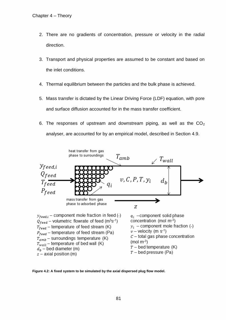
Chapter 4 – Theory
81
2. There are no gradients of concentration, pressure or velocity in the radial
direction.
3. Transport and physical properties are assumed to be constant and based on
the inlet conditions.
4. Thermal equilibrium between the particles and the bulk phase is achieved.
5. Mass transfer is dictated by the Linear Driving Force (LDF) equation, with pore
and surface diffusion accounted for in the mass transfer coefficient.
6. The responses of upstream and downstream piping, as well as the CO2
analyser, are accounted for by an empirical model, described in Section 4.9.
Figure 4.2: A fixed system to be simulated by the axial dispersed plug flow model.

Chapter 4 – Theory
82
The use of the ideal gas law is justified by Casas et al. (2012) for a high pressure
system based on the compressibility of the gas mixture being above 0.9. The Peng-
Robinson equation of state was used to find the compressibility of the feed stream
and this assumption was found to be valid for all possible gas mixtures, these results
are detailed in Appendix G. Shafeeyan et al. (2014) reported that assuming there
are no radial gradients is well defined in literature. The assumptions which place the
particles in thermal equilibrium with the bulk phase has been taken as there is
insufficient data to validate the temperature differences. Pore diffusion and surface
diffusion models are not used as they have been shown in literature to have little
effect as long as the typical S-shape of the breakthrough curve is observed (Liaw et
al., 1979).
4.6.1 Mass Balance
The component and overall mass balance used are presented in Table 4.6 and were
derived from a differential mass balance over an element of a fixed bed (Ruthven,
1984). Both equations have four parts: an accumulation term, a convective term, a
dispersive term and an adsorption term presented in that order. The component
mass balance in Equation 4.23 combines the overall mass balance and a mass
balance of component i as detailed by Ko et al. (2005) and shown in Appendix H.
The voidages have been assigned respectively to total voidage (휀𝑡) and bed voidage
(휀𝑏) following Casas et al. (2012). Supplementary equations were needed to specify
the concentration and voidages. The total concentration was calculated using the
ideal gas law in Equation 4.24 and the component concentration was related to the

Chapter 4 – Theory
83
total concentration by the mole fraction in Equation 4.25. The total voidage was
calculated from the specified bed voidage and particle voidage (휀𝑝) by Equation 4.26.
Table 4.6: Mass balance equations for the axial dispersed plug flow model and supplementary equations
Overall 휀𝑡𝜕𝐶
𝜕𝑡= −휀𝑏
𝜕(𝐶𝑣)
𝜕𝑧+ 휀𝑏𝐷𝑎𝑥
𝜕2𝐶
𝜕𝑧2− 𝜌𝑏∑
𝜕𝑞𝑖𝜕𝑡
𝑛
𝑖=1
4.22
Component
휀𝑡𝜕𝑦𝑖𝜕𝑡= −휀𝑏𝑣
𝜕𝑦𝑖𝜕𝑧+ 휀𝑏𝐷𝑎𝑥 (
𝜕2𝑦𝑖𝜕𝑧2
+2
𝐶
𝜕𝑦𝑖𝜕𝑧
𝜕𝐶
𝜕𝑧)
−𝜌𝑏𝐶(𝜕𝑞𝑖𝜕𝑡− 𝑦𝑖∑
𝜕𝑞𝑖𝜕𝑡
𝑛
𝑖=1
)
4.23
Ideal Gas Law
𝐶 =𝑃
𝑅𝑇
4.24
Component Concentration
𝑐𝑖 = 𝐶 𝑦𝑖 4.25
Total Voidage 휀𝑡 = 휀𝑏 + 휀𝑝 − 휀𝑏휀𝑝 4.26
4.6.2 Energy Balance
An energy balance is required if the system is non-isothermal. There are three main
types of energy balance: non-isothermal without wall effects, adiabatic and
non-isothermal with wall effects. For a non-isothermal system without wall effects the
additional assumptions that thermal equilibrium between the bed wall and the
surroundings is attained and that the surrounding temperature is constant are
required.
The energy balances which dictate these three operating modes are given in Table
4.7 by Equations 4.27 to 4.29. These all include an accumulation term, a convective
flux, a dispersive flux and an energy generation term. The difference between them is
in the last term where the energy dissipation out of the system is described. For the
system without wall effects this is described by heat transfer to the surroundings, for
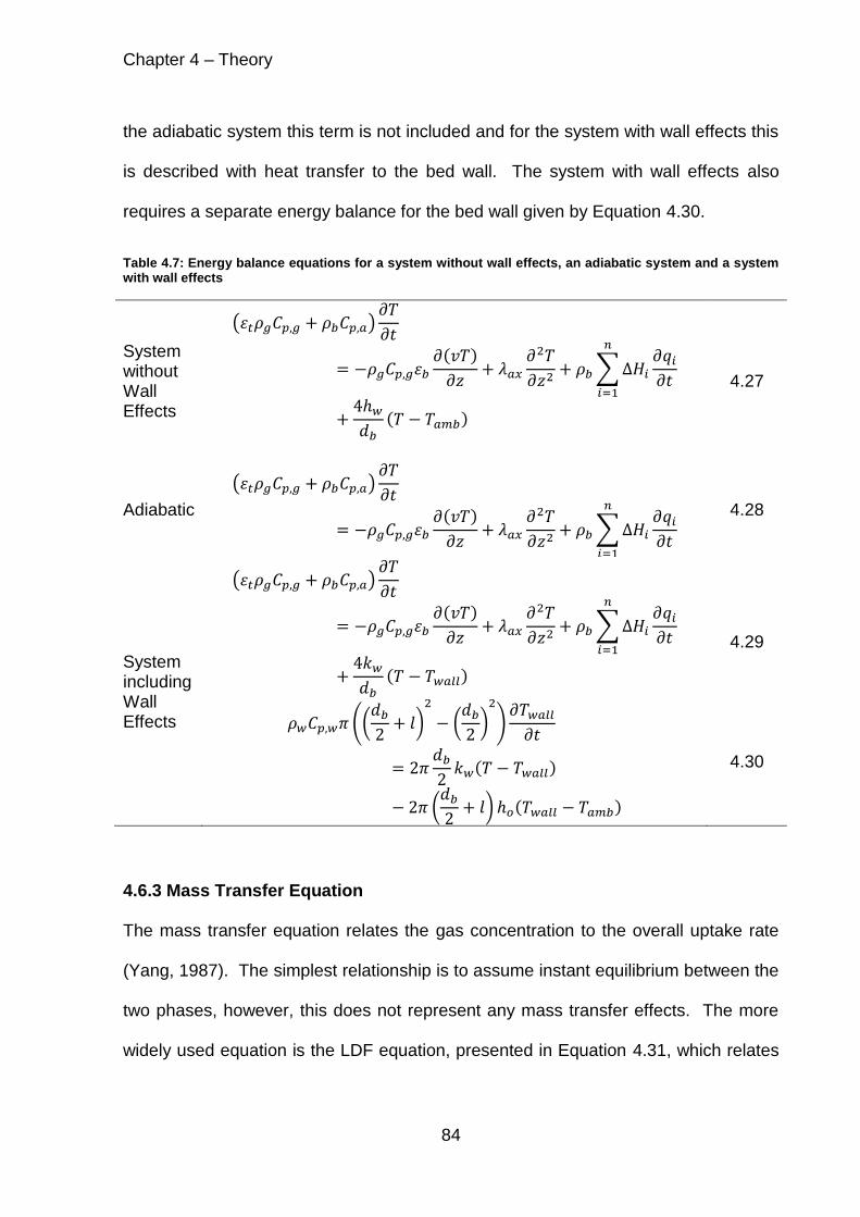
Chapter 4 – Theory
84
the adiabatic system this term is not included and for the system with wall effects this
is described with heat transfer to the bed wall. The system with wall effects also
requires a separate energy balance for the bed wall given by Equation 4.30.
Table 4.7: Energy balance equations for a system without wall effects, an adiabatic system and a system with wall effects
System without Wall Effects
(휀𝑡𝜌𝑔𝐶𝑝,𝑔 + 𝜌𝑏𝐶𝑝,𝑎)𝜕𝑇
𝜕𝑡
= −𝜌𝑔𝐶𝑝,𝑔휀𝑏𝜕(𝑣𝑇)
𝜕𝑧+ 𝜆𝑎𝑥
𝜕2𝑇
𝜕𝑧2+ 𝜌𝑏∑∆𝐻𝑖
𝜕𝑞𝑖𝜕𝑡
𝑛
𝑖=1
+4ℎ𝑤𝑑𝑏
(𝑇 − 𝑇𝑎𝑚𝑏)
4.27
Adiabatic
(휀𝑡𝜌𝑔𝐶𝑝,𝑔 + 𝜌𝑏𝐶𝑝,𝑎)𝜕𝑇
𝜕𝑡
= −𝜌𝑔𝐶𝑝,𝑔휀𝑏𝜕(𝑣𝑇)
𝜕𝑧+ 𝜆𝑎𝑥
𝜕2𝑇
𝜕𝑧2+ 𝜌𝑏∑∆𝐻𝑖
𝜕𝑞𝑖𝜕𝑡
𝑛
𝑖=1
4.28
System including Wall Effects
(휀𝑡𝜌𝑔𝐶𝑝,𝑔 + 𝜌𝑏𝐶𝑝,𝑎)𝜕𝑇
𝜕𝑡
= −𝜌𝑔𝐶𝑝,𝑔휀𝑏𝜕(𝑣𝑇)
𝜕𝑧+ 𝜆𝑎𝑥
𝜕2𝑇
𝜕𝑧2+ 𝜌𝑏∑∆𝐻𝑖
𝜕𝑞𝑖𝜕𝑡
𝑛
𝑖=1
+4𝑘𝑤𝑑𝑏
(𝑇 − 𝑇𝑤𝑎𝑙𝑙)
𝜌𝑤𝐶𝑝,𝑤𝜋 ((𝑑𝑏2+ 𝑙)
2
− (𝑑𝑏2)2
)𝜕𝑇𝑤𝑎𝑙𝑙𝜕𝑡
= 2𝜋𝑑𝑏2𝑘𝑤(𝑇 − 𝑇𝑤𝑎𝑙𝑙)
− 2𝜋 (𝑑𝑏2+ 𝑙) ℎ𝑜(𝑇𝑤𝑎𝑙𝑙 − 𝑇𝑎𝑚𝑏)
4.29
4.30
4.6.3 Mass Transfer Equation
The mass transfer equation relates the gas concentration to the overall uptake rate
(Yang, 1987). The simplest relationship is to assume instant equilibrium between the
two phases, however, this does not represent any mass transfer effects. The more
widely used equation is the LDF equation, presented in Equation 4.31, which relates

Chapter 4 – Theory
85
the two phases by a single mass transfer resistance. This has been shown to be
sufficient for simple adsorption processes (Liaw et al., 1979).
Table 4.8: Linear driving force equation
LDF 𝜕𝑞𝑖𝜕𝑡= 𝑘𝑖(𝑞𝑖
∗ − 𝑞𝑖) 4.31
4.6.4 Pressure Drop
The pressure drop across the bed is given by the modified Ergun equation presented
in Equations 4.32 to 4.34. The ratio of particle diameter (𝑑𝑝) to bed diameter (𝑑𝑏) is
25 and the wall effects must be taken into account when this ratio is less than 50
(Mehta and Hawley, 1969), requiring the modified Ergun equation to be used instead
of the standard Ergun equation.
Table 4.9: Pressure drop across the bed described the modified Ergun equation
Modified Ergun Equation
−𝜕𝑃
𝜕𝑧= 150𝜇𝑔𝑣
(1 − 휀𝑏)2
𝑑𝑝2휀𝑏
3+ 1.75𝜌𝑔𝑣|𝑣|
(1 − 휀𝑏)
𝑑𝑝휀𝑏3
𝐴𝑒𝑟𝑔 = 150 (1 +2𝑑𝑝
3𝑑𝑏(1 − 휀𝑏))
2
𝐵𝑒𝑟𝑔 = 1.75 (1 +2𝑑𝑝
3𝑑𝑏(1 − 휀𝑏))
4.32
4.33
4.34
4.7 Correlations
The equations presented in Section 4.6 describe the interactions in the system but
parameter values are needed to characterise the system within the model. The
majority of properties are gas or adsorbent properties that were found by
independent experiment or from literature values. There are, however, some
properties which are dependent on the interaction between the gas and the
adsorbent and it is difficult to find values independently. These parameters include
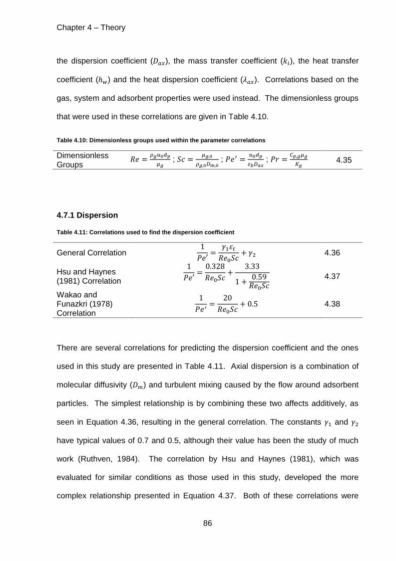
Chapter 4 – Theory
86
the dispersion coefficient (𝐷𝑎𝑥), the mass transfer coefficient (𝑘𝑖), the heat transfer
coefficient (ℎ𝑤) and the heat dispersion coefficient (𝜆𝑎𝑥). Correlations based on the
gas, system and adsorbent properties were used instead. The dimensionless groups
that were used in these correlations are given in Table 4.10.
Table 4.10: Dimensionless groups used within the parameter correlations
Dimensionless Groups
𝑅𝑒 =𝜌𝑔𝑢0𝑑𝑝
𝜇𝑔 ; 𝑆𝑐 =
𝜇𝑔,0
𝜌𝑔,0𝐷𝑚,0 ; 𝑃𝑒′ =
𝑢0𝑑𝑝
𝜀𝑏𝐷𝑎𝑥 ; 𝑃𝑟 =
𝐶𝑝,𝑔𝜇𝑔
𝐾𝑔 4.35
4.7.1 Dispersion
Table 4.11: Correlations used to find the dispersion coefficient
General Correlation 1
𝑃𝑒′=𝛾1휀𝑡𝑅𝑒0𝑆𝑐
+ 𝛾2 4.36
Hsu and Haynes (1981) Correlation
1
𝑃𝑒′=0.328
𝑅𝑒0𝑆𝑐+
3.33
1 +0.59𝑅𝑒0𝑆𝑐
4.37
Wakao and Funazkri (1978) Correlation
1
𝑃𝑒′=
20
𝑅𝑒0𝑆𝑐+ 0.5 4.38
There are several correlations for predicting the dispersion coefficient and the ones
used in this study are presented in Table 4.11. Axial dispersion is a combination of
molecular diffusivity (𝐷𝑚) and turbulent mixing caused by the flow around adsorbent
particles. The simplest relationship is by combining these two affects additively, as
seen in Equation 4.36, resulting in the general correlation. The constants 𝛾1 and 𝛾2
have typical values of 0.7 and 0.5, although their value has been the study of much
work (Ruthven, 1984). The correlation by Hsu and Haynes (1981), which was
evaluated for similar conditions as those used in this study, developed the more
complex relationship presented in Equation 4.37. Both of these correlations were

Chapter 4 – Theory
87
developed for non-porous particles, but Wakao and Funazkri (1978) found that for
porous particles under adsorbing conditions the dispersion was much greater than
predicted by previous correlations, especially at low Reynolds numbers. They
instead suggested the correlation presented by Equation 4.38 which predicts much
higher dispersion at low Reynolds numbers. All three of these correlations are
evaluated in Section 6.3.2.2.
4.7.2 Mass Transfer Coefficient
Table 4.12: Correlations for calculating the mass transfer coefficient
Mass Transfer Coefficient
1
𝑘𝑖=𝑑𝑝𝑞0,𝑖
6𝑘𝑓𝑐0,𝑖+
𝑑𝑝𝑜𝑟𝑒2 𝑞0,𝑖
60휀𝑝𝐷𝑝𝑜𝑟𝑒𝑐0,𝑖+
𝑟𝑐2
15𝐷𝑐 4.39
Surface Mass Transfer
𝑘𝑓 =𝐷𝑚𝑑𝑝(2.0 + 1.1𝑅𝑒0.6𝑆𝑐1 3⁄ ) 4.40
Pore Diffusivity
𝐷𝑝𝑜𝑟𝑒 =휀𝑝𝐷𝑘𝐷𝑚
𝜏(𝐷𝑘 + 𝐷𝑚)
𝐷𝑘 = 9700𝑑𝑝𝑜𝑟𝑒
2(𝑇
𝑀𝑤)
12⁄
𝐷𝑚 = 0.0018583√𝑇3 (1
𝑀𝑤,𝐴+
1
𝑀𝑤,𝐵)
1
𝑃𝜎𝐴𝐵2 𝛺𝐷,𝐴𝐵
𝜎𝐴𝐵 =1
2(𝜎𝐴 + 𝜎𝐴)
휀𝐴𝐵 = √휀𝐴휀𝐵
𝑇𝑑𝑖𝑚 =𝜅𝑇
휀𝐴𝐵
4.41
4.42
4.43
4.44
4.45
4.46
The use of the LDF model as the only description of the mass transfer requires the
mass transfer coefficient to incorporate all three mass transfer resistances, namely
external mass transfer (𝑘𝑓), pore diffusion (𝐷𝑝𝑜𝑟𝑒) and micropore diffusion (𝐷𝑐). All of
the equations used in this study to calculate the mass transfer coefficient are
reported in Table 4.12. The correlation used by Farooq and Ruthven (1990) for the

Chapter 4 – Theory
88
mass transfer coefficient incorporates the three mass transfer resistances and is
presented in Equation 4.39. The external mass transfer coefficient was found using
the correlation, Equation 4.40, suggested by Wakao and Funazkri (1978). The
diffusivity was found from the Chapman-Enskog equation, Equation 4.43, as given by
Bird et al. (2001) and the Knudsen diffusion (𝐷𝑘) was calculated using Equation 4.42
(Nikolic et al., 2008). The pore diffusion was then calculated by combining the effect
of the Knudsen diffusion and diffusivity by Equation 4.41 (Nikolic et al., 2008). There
are no suitable correlations for finding the micropore diffusivity used in the third term
of Equation 4.39 and so in this study the values reported by Shen et al. (2010) are
used.
4.7.3 Heat Balance Coefficients
Table 4.13 reports the correlations needed for the heat transfer coefficient, the heat
dispersion coefficient for all energy balances considered and a further correlation for
the external heat transfer coefficient, which is needed for a system that considers the
wall effects. The heat transfer coefficient is predicted using either the Yagi and Kunii
(1960) correlation, Equation 4.47, or the Leva (1947) correlation, Equation 4.48, with
the merits of each equation discussed in Section 6.3.2.4. The heat dispersion
coefficient is predicted using the Wakao et al. (1979) correlation, Equation 4.49. The
external heat transfer from the bed wall to the surrounding air (ℎ𝑜) is assumed to be
natural convection and is described by the Nusselt equation, Equation 4.50, which is
based on the Grashoff number, Equation 4.51, and the Prandtl number for a
horizontal cylinder with 𝑎 = 0.53 and 𝑚 = 0.25 (Perry et al., 1997).

Chapter 4 – Theory
89
Table 4.13: Correlations used for parameters in the energy balance
Yagi and Kunii (1960) Correlation
ℎ𝑤 = ℎ𝑤𝑜 + 𝛼𝑤(𝐶𝑝,𝑔𝜌𝑔𝑢)
4.47
Leva (1947) Correlation
ℎ𝑤 =0.813𝑅𝑒0.9𝐾𝑔
𝑑𝑏𝑒(
−6𝑑𝑝
𝑑𝑏⁄
)
4.48
Heat Dispersion Coefficient
𝜆𝑎𝑥 = 𝐾𝑔(7 + 0.5𝑃𝑟𝑅𝑒) 4.49
External Heat Transfer Coefficient
ℎ𝑜 =𝐾𝑎𝑖𝑟
(𝑑𝑏 + 2𝛿)𝑎(𝐺𝑟𝑎𝑖𝑟𝑃𝑟𝑎𝑖𝑟)
𝑚
𝐺𝑟 =𝑔𝛽(𝑇𝑤𝑎𝑙𝑙 − 𝑇𝑎𝑖𝑟)(𝑑𝑏 + 2𝛿)
3
(𝜇𝜌⁄ )2
𝛽𝑎𝑖𝑟 =1
𝑇𝑎𝑖𝑟
4.50
4.51
4.52
4.8 Boundary and Initial Conditions
The boundary conditions are presented in Table 4.14. They are based on the well
known Danckwert’s Boundary conditions (Danckwerts, 1953) and the conditions of
the inlet stream. These represent the reactor as a closed system and allow for the
flow just inside the reactor to take into account convection and diffusion.
Table 4.14: Model Boundary Conditions
Boundary Conditions
−𝐷𝑎𝑥𝜕𝑦𝑖𝜕𝑡|𝑧=0
= 𝑣|𝑧=0(𝑦𝑓𝑒𝑒𝑑 − 𝑦𝑖|𝑧=0)
𝑃|𝑧=0 = 𝑃𝑓𝑒𝑒𝑑; 𝑇|𝑧=0 = 𝑇𝑓𝑒𝑒𝑑; 𝑣|𝑧=0 =𝑄𝑓𝑒𝑒𝑑
𝐴휀𝑡
𝜕𝑇
𝜕𝑧|𝑧=𝐿
= 0; 𝜕𝑃
𝜕𝑧|𝑧=𝐿
= 0; 𝜕𝑦𝑖𝜕𝑧|𝑧=𝐿
= 0; 𝜕𝑣
𝜕𝑧|𝑧=𝐿
= 0
4.53
The initial conditions which describe the state of the bed at time zero are given in
Table 4.15. They assume that initially the flow through the bed is the same as the
feed flow and that the only gas in the bed is nitrogen. They also state that the

Chapter 4 – Theory
90
adsorbed state is not changing and as the bed is saturated with nitrogen, neither is
the adsorbed state.
Table 4.15: Model Initial Conditions
Initial Conditions
𝜕𝑞𝑖𝜕𝑡= 0
𝑦𝐶𝑂2 = 0; 𝑦𝑁2 = 1
𝑣 =𝑄𝑓𝑒𝑒𝑑
𝐴휀𝑡
4.54
4.9 Empirical System Model
The model described in Section 4.6 describes an adsorption bed but it does not
simulate the response of the surrounding system. The piping system that connects
the adsorption bed in the experimental set-up, described in Figure 3.7, is complex
with many valves and pipe bends and is difficult to simulate with simple theoretical
models. The response of the piping system is found through independent
experiments described in Section 3.6.2. A model based on the axial dispersed plug
flow model of a simplified bed is used to replicate the produced experimental
breakthrough curves. The model assumes that the bed velocity, pressure and
temperature are all fixed and that no adsorption takes place. This reduces Equations
4.22, 4.23, 4.27 and 4.31 to Equations 4.55 to 4.58 presented in Table 4.16.
Table 4.16: Reduced axial dispersed plug flow model for simulating system surrounding the adsorption bed
Empirical Model
𝜕𝑦𝑖𝜕𝑡= −𝑣
𝜕𝑦𝑖𝜕𝑧+ 𝐷𝑎𝑥
𝜕2𝑦𝑖𝜕𝑧2
𝜕𝑣
𝜕𝑧= 0
𝑇 = 𝑇𝑓𝑒𝑒𝑑
𝑃 = 𝑃𝑓𝑒𝑒𝑑
4.55
4.56
4.57 4.58

Chapter 4 – Theory
91
In order to fit the breakthrough curves for a system without an adsorption bed, a
model was established with the configuration shown in Figure 4.3. The fitting of the
simulation output to the experimental breakthrough curves was achieved by using the
Parameter Estimation tool within gProms. Within the system the bed area and
dispersion coefficient were used as fitting parameters for each of the bed models.
The parameters found were empirical with accurate replication of experimental
breakthrough curves the main concern. This was done by first fitting beds 1 and 2 to
the output of the response of the CO2 analyser described in Section 3.6.1. The
parameters in these beds were then fixed and the beds were connected in a model to
beds 3 and 4. The process was repeated using parameters within beds 3 and 4 in the
Parameter Estimation tool to match the output of the system without a bed described
in Section 3.6.2.
Figure 4.3: Configuration of empirical models for simulating the response of the system surrounding the adsorption bed
4.10 Solver Implementation
The solution method used is important in ensuring the stability and the accuracy of
the model. The solution methods in gProms use method of lines numerical solvers.
The main reactor bed used a second order backward finite difference method with 30
elements. The backward finite difference method is used to oppose the direction of
flow and the second order nature ensures the accuracy of the system (LeVaque,
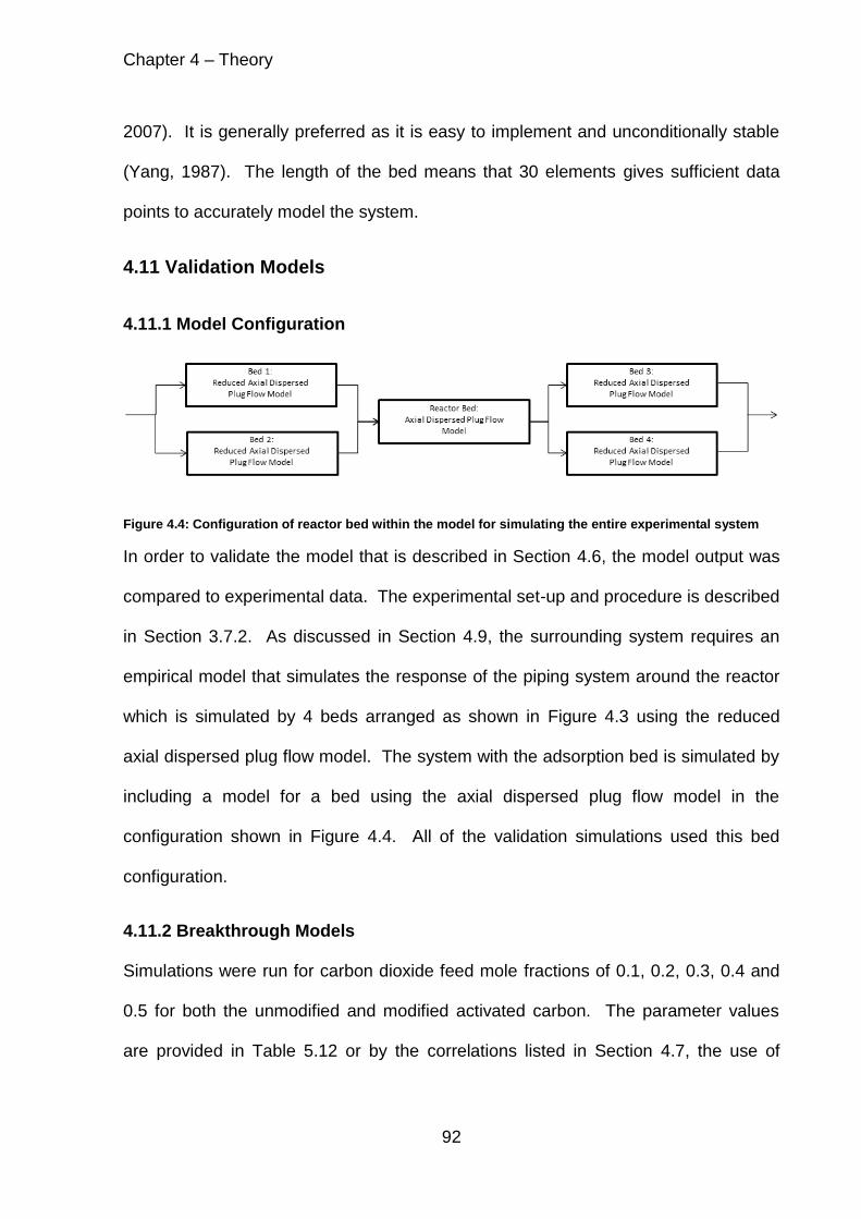
Chapter 4 – Theory
92
2007). It is generally preferred as it is easy to implement and unconditionally stable
(Yang, 1987). The length of the bed means that 30 elements gives sufficient data
points to accurately model the system.
4.11 Validation Models
4.11.1 Model Configuration
Figure 4.4: Configuration of reactor bed within the model for simulating the entire experimental system
In order to validate the model that is described in Section 4.6, the model output was
compared to experimental data. The experimental set-up and procedure is described
in Section 3.7.2. As discussed in Section 4.9, the surrounding system requires an
empirical model that simulates the response of the piping system around the reactor
which is simulated by 4 beds arranged as shown in Figure 4.3 using the reduced
axial dispersed plug flow model. The system with the adsorption bed is simulated by
including a model for a bed using the axial dispersed plug flow model in the
configuration shown in Figure 4.4. All of the validation simulations used this bed
configuration.
4.11.2 Breakthrough Models
Simulations were run for carbon dioxide feed mole fractions of 0.1, 0.2, 0.3, 0.4 and
0.5 for both the unmodified and modified activated carbon. The parameter values
are provided in Table 5.12 or by the correlations listed in Section 4.7, the use of

Chapter 4 – Theory
93
which are discussed in Section 6.3.2. The operation of the models is controlled to
match the experimental procedure described in Section 3.7.2. For the breakthrough
models there are no changes in the input conditions and therefore the simulation is
based on the initial conditions and the boundary conditions outlined in Section 4.8
and the model is run for the same length of time as the experiment,
i.e. 5400 seconds.
4.11.3 Cyclic Models
The 3 step and 4 step models required for simulating the experiments described in
Section 3.7.3 and 3.7.4 respectively are more complex as the feed conditions of the
system change depending on the step.
Table 4.17: Relationship for changing the flowrate in pressure swing adsorption cycles.
Feed Flowrate
𝜕𝑄
𝜕𝑡= 𝑐𝑜𝑛𝑠𝑡𝑎𝑛𝑡 4.59
It is necessary to build the change of conditions for each step into the simulation.
Three of the feed conditions can change when the system switches to the next step:
the mole fraction of each gas, the flowrate and the pressure. The mole fraction was
changed by introducing a discontinuity into the system by reassigning the values in
the simulation. The flowrate and pressure on the other hand could not be changed
by reassigning the value as the solver was not able to incorporate the discontinuity.
The flowrate changes in the 4 step model were achieved by a linear relationship as
described by Equation 4.59 in Table 4.17. The constant used in that equation was
the difference between the final flowrate and the initial flowrate divided by the time for
the flowrate change to take place.

Chapter 4 – Theory
94
The bed pressure is more difficult to control. This is often done using a pressure
profile (Cen and Yang, 1986; Yang and Doong, 1985). It was not possible to
implement a linear relationship similar to the one used for the flowrate as used by Ko
et al. (2005) because this led to a rapidly increasing exit velocity with a large spike for
a depressurisation time of 60 seconds, which is unrealistic and can cause errors in
the simulation. Instead a control system was used to maintain a constant flowrate at
the bed exit. This has previously been achieved using a control valve equation, such
as Equation 4.68, in order to connect models (Choi and Wen-Chung, 1994; Nikolic et
al., 2008). However the produced system where the exit flowrate is set as a
boundary condition becomes too stiff and was not able to solve.
Table 4.18: Equations used on the control of the bed pressure
Valve Equation
𝑄 = 𝐶𝑣. 𝑆𝑃. √∆𝑃2
𝑆𝐺𝑔 4.60
Bed Pressure
𝜕𝑃
𝜕𝑡= −𝑑𝑒𝑝𝑟𝑒𝑠𝑠 𝑟𝑎𝑡𝑒
𝐸𝑟𝑟𝑜𝑟 = 𝑃𝑜𝑢𝑡 𝑠𝑒𝑡 − 𝑃𝑜𝑢𝑡 𝑑𝑒𝑝𝑟𝑒𝑠𝑠 𝑟𝑎𝑡𝑒 = 𝑑𝑒𝑝𝑟𝑒𝑠𝑠 𝑟𝑎𝑡𝑒
× (𝐸𝑟𝑟𝑜𝑟 × 𝑃𝑟𝑜𝑝𝑜𝑟𝑡𝑖𝑜𝑛 𝐶𝑜𝑛𝑠𝑡𝑎𝑛𝑡 + 1)
4.61
4.62 4.63
This work instead set the rate of change of pressure to a variable, Equation 4.61,
which was then controlled in a while loop. The while loop, shown in Figure 4.5,
maintains the exit flowrate whilst the bed is depressurising by comparing the exit
flowrate to the desired flowrate and then reducing the depressurisation rate if the exit
flowrate is too high. The depressurisation rate was not manipulated if the flowrate is
too low, but instead maintained for that iteration as a constant depressurisation rate
produces a rising flowrate profile. The equations used for this are given in Table

Chapter 4 – Theory
95
4.18, with the depressurisation rate manipulated in Equation 4.63 based on the
difference between the set pressure and actual pressure given in Equation 4.62.
Simulations were run to match the experiments described in Section 3.7.3. For both
cases the pressurisation step was not simulated as the experimental outputs during
this step remain constant and therefore comparison of the simulation with them
would be meaningless. Instead, the systems were assumed to start with the
adsorption step with the same conditions as for the breakthrough model. For the 3
step model, carbon dioxide feed mole fractions of 0.1, 0.2, 0.3, 0.4 and 0.5 were
simulated for both the unmodified and modified activated carbon. The operation of
the beds in a 3 step system is shown in Figure 4.6a, with the regeneration step split
into two beds so as to clearly show the 60 second depressurisation that occurs at the
start of this step. The cycle time varied depending on the carbon dioxide feed mole
fraction. The adsorption step for carbon dioxide feed fraction of 0.1 is 5400 seconds,
for 0.2 is 4500 seconds and for 0.3 – 0.5 are 3600 seconds to match the
experimental runs. For all cases the regeneration step was 2700 seconds, with a 60
second depressurisation followed by a 2640 second purge.
Figure 4.5: While loop for controlling the bed exit flowrate during depressurisation

Chapter 4 – Theory
96
Simulations were run for the 4 step system using a carbon dioxide feed fraction of 0.4
for both the unmodified and modified activated carbon. The operation of the 4 step
process is shown in Figure 4.6b. In order to match the experiments described in
Section 3.7.4, the adsorption step was run for 1510 seconds for the unmodified
activated carbon and 1260 seconds for the modified activated carbon, the blowdown
step was run for 600 seconds, with the depressurisation occurring in the first 60
seconds, and the purge step for 2100 seconds.
Figure 4.6: Operation steps for the a) 3 step cycle and b) 4 step cycle
4.11.4 Performance Indicator
The experimental and simulation breakthrough curves were compared numerically by
using the normalised sum of the squared differences (SSD) between the
experimental mole fraction at a set time and the simulation output for that time. The
normalised version was used so that systems with a different number of data points
could be compared. The sum of the squared of the differences has been used
previously by Won et al. (2012) for the same comparison. It should be noted that the
graphs should also be compared qualitatively as a lower SSD can be found for a
system that is a poorer fit to the shape of a breakthrough curve (Won et al., 2012).

Chapter 4 – Theory
97
Table 4.19: Equation for the normalised sum of the squared differences
Normalised sum of the squared differences 𝑆𝑆𝐷 = (
∑(𝑦𝑖,𝑒𝑥𝑝 − 𝑦𝑖,𝑚𝑜𝑑)2
𝑁 − 1)
0.5
4.64
4.12 Pressure Swing Adsorption Models
The validated model was used to simulate several PSA systems, which are detailed
in their individual sections in Chapter 7. They were all based on the axial dispersed
plug flow model, surrounding equations and assumptions detailed in Section 4.6 as
well as the boundary and initial conditions outlined in Sections 4.8. The empirical
system model was not included as only the adsorption bed is simulated, not the
surrounding system from the experimental set-up.
4.12.1 Model Set-up and Solvers Used
PSA models involve connecting multiple beds together. This was achieved by
building models which combine multiple beds based on the same underlying
adsorption model. The feed conditions to each bed were the only aspects
manipulated based on the PSA step each bed was operating under. For steps where
beds are connected to each other, e.g. pressure equalisation, the feed conditions of
the downstream bed were set to the outlet conditions of the upstream bed. The
switching between steps was achieved in the same way as for the validation models.
Changes to feed mole fraction were implemented by introducing a discontinuity and
reassigning the value. Changes in flowrate were achieved using the linear
relationship given by Equation 4.59. For beds that are interconnected, the flowrate of
each bed was manipulated to be the same and then the connection was
implemented so as to avoid large discontinuities. Depressurisation was controlled by

Chapter 4 – Theory
98
maintaining a constant exit flowrate using the control loop described by Figure 4.5
and the equations from Table 4.18.
Table 4.20: Equations for controlling bed pressurisation
Bed Pressure
𝜕𝑃
𝜕𝑡= 𝑟𝑒𝑝𝑟𝑒𝑠𝑠 𝑟𝑎𝑡𝑒
𝐸𝑟𝑟𝑜𝑟 = 𝑄𝑜𝑢𝑡 − 𝑄𝑜𝑢𝑡 𝑠𝑒𝑡 𝑟𝑒𝑝𝑟𝑒𝑠𝑠 𝑟𝑎𝑡𝑒 = 𝑟𝑒𝑝𝑟𝑒𝑠𝑠 𝑟𝑎𝑡𝑒
× (𝐸𝑟𝑟𝑜𝑟 × 𝑃𝑟𝑜𝑝𝑜𝑟𝑡𝑖𝑜𝑛 𝐶𝑜𝑛𝑠𝑡𝑎𝑛𝑡 + 1)
4.65
4.66 4.67
The pressurisation steps were controlled in the same manner as the depressurisation
steps. Changing the boundary conditions to set the exit flowrate to 0 m3 s-1 makes
the system stiff and difficult to solve. Instead a similar control loop to that described
in Figure 4.5 was used but instead the 𝑟𝑒𝑝𝑟𝑒𝑠𝑠 𝑟𝑎𝑡𝑒 was controlled and was
increased if the outlet flowrate was above the set value and was reduced if the outlet
flowrate was below the set value. Computationally, zero is difficult to implement and
therefore the outlet flowrate is set to two orders of magnitude below the overall feed
flowrate. The equations used in the control are provided in Table 4.20.
The number of beds simulated was dependent on the system. For system where
there are no interconnections between the beds, only one bed is modelled. All other
beds are then assumed to have the same outputs but starting from a different step.
Systems where beds are connected require all of the beds in the system to be
simulated. The exception to this is for a 6 step system using one equalisation step
as the cycles match in such a way that 3 bed pairs are formed which do not interact
with other bed pairs. Therefore only one bed pair was simulated.

Chapter 4 – Theory
99
Figure 4.7: While loop for controlling the bed exit flowrate during pressurisation
The solvers used for co-current flow are described in Section 4.10. Some models
operated with co-current and counter-current flow, with counter-current operation
requiring the ends that the boundary conditions apply to be switched. The forward
finite difference method was used for these steps instead of the backward finite
difference method to match the change in direction of flow.
4.12.2 Performance Indicators
Table 4.21: Carbon dioxide and nitrogen capture rates and purities
Purities and Capture Rates
𝐶𝑂2 𝑃𝑢𝑟𝑖𝑡𝑦 = ∫ 𝐹𝐶𝑂2
𝑜𝑢𝑡𝑑𝑡𝑝𝑢𝑟𝑔𝑒
+ ∫ 𝐹𝐶𝑂2𝑜𝑢𝑡𝑑𝑡
𝑏𝑙𝑜𝑤
∫ (𝐹𝐶𝑂2𝑜𝑢𝑡 + 𝐹𝑁2
𝑜𝑢𝑡)𝑑𝑡𝑝𝑢𝑟𝑔𝑒
+ ∫ (𝐹𝐶𝑂2𝑜𝑢𝑡 + 𝐹𝑁2
𝑜𝑢𝑡)𝑑𝑡𝑏𝑙𝑜𝑤
𝐶𝑂2 𝐶𝑎𝑝𝑡𝑢𝑟𝑒 𝑅𝑎𝑡𝑒 = ∫ 𝐹𝐶𝑂2
𝑜𝑢𝑡𝑑𝑡𝑝𝑢𝑟𝑔𝑒
+ ∫ 𝐹𝐶𝑂2𝑜𝑢𝑡𝑑𝑡
𝑏𝑙𝑜𝑤
∫ 𝐹𝐶𝑂2𝑖𝑛 𝑑𝑡
𝑝𝑢𝑟𝑔𝑒+ ∫ 𝐹𝐶𝑂2
𝑖𝑛 𝑑𝑡𝑎𝑑𝑠
+ ∫ 𝐹𝐶𝑂2𝑖𝑛 𝑑𝑡
𝑝𝑟𝑒𝑠𝑠
𝑁2 𝑃𝑢𝑟𝑖𝑡𝑦 = ∫ 𝐹𝑁2
𝑜𝑢𝑡𝑑𝑡𝑎𝑑𝑠
∫ (𝐹𝐶𝑂2𝑜𝑢𝑡 + 𝐹𝑁2
𝑜𝑢𝑡)𝑑𝑡𝑎𝑑𝑠
𝑁2 𝐶𝑎𝑝𝑡𝑢𝑟𝑒 𝑅𝑎𝑡𝑒 = ∫ 𝐹𝑁2
𝑜𝑢𝑡𝑑𝑡𝑎𝑑𝑠
∫ 𝐹𝑁2𝑖𝑛𝑑𝑡
𝑝𝑢𝑟𝑔𝑒+ ∫ 𝐹𝑁2
𝑖𝑛𝑑𝑡𝑎𝑑𝑠
+ ∫ 𝐹𝑁2𝑖𝑛𝑑𝑡
𝑝𝑟𝑒𝑠𝑠
4.68 4.69 4.70 4.71

Chapter 4 – Theory
100
It is necessary to use performance indicators to describe the effectiveness of the
separation achieved by the PSA processes evaluated. The gas purities and capture
rates were used to establish the viability of a process (Grande, 2012) and the
equations to calculate these values are presented in Table 4.21. The gas purity is
the volume averaged concentration of the product streams as the nature of PSA
means that the outlet concentrations of the gases will not be constant (Yang, 1987)
and reflects the quality of the gas produced. It was calculated by Equation 4.68 for
carbon dioxide and by Equation 4.70 for nitrogen. In both cases it is the amount of
the desired gas collected in the steps which that gas is produced as product divided
by the amount of gas produced in those steps. The capture rate is the commonly
used term to refer to the percentage of the gas input into the system that is captured,
also referred to as recovery in literature. It is the amount of the desired gas collected
in the steps which that gas is produced as product divided by the amount of the
desired gas that is input into the system. This reflects the efficiency of the process.
The carbon dioxide capture rate was calculated using Equation 4.69 and the nitrogen
capture rate by Equation 4.71.
The theory presented in this chapter outlines the equations used to describe
adsorption processes. The implementation of these equations has been described to
show the models built to simulate these processes. The results chapters discuss the
suitability of their implementation.

Chapter 5 – Evaluation of Activated Carbon Materials and their Dynamic Capacities
101
Chapter 5 – Evaluation of Activated Carbon Materials and their
Dynamic Capacities
Chapter 5 – Evaluation of Activated Carbon Materials and their Dynamic Capacities
102
5.1 Introduction
It is necessary to investigate adsorbent materials experimentally in order to obtain
the necessary data to design and improve pressure swing adsorption (PSA)
processes. These materials need to be investigated under conditions similar to those
used on an industrial scale. Adsorbent materials are typically studied under
equilibrium conditions using pure gases only. However, since a PSA unit typically
applied for industrial separations would not reach full saturation, adsorbent capacity
for carbon dioxide under dynamic conditions from gas mixtures needs to be studied.
This gives a more realistic estimate of the potential uptake of carbon dioxide and
facilitates scale up of the process. The work on this in the literature has been
relatively limited for high pressure separations, with few authors attempting to
connect the dynamic capacity to the performance of the material. García et al.
(2011) and Grande et al. (2013) in separate studies look at the dynamic capacity
without evaluating the equilibrium capacity. Several works have studied the dynamic
response of the system without actually evaluating the adsorbent capacity (Casas et
al., 2012; Lopes et al., 2009; Lopes et al., 2011; Shen et al., 2010). Many studies
have looked at the pure component capacity but only a few have evaluated the
multicomponent capacities of activated carbons at high pressure (Dreisbach et al.,
1999; García et al., 2013; Schell et al., 2012b). Therefore further work is required to
evaluate the effectiveness of equilibrium experiments and to suggest the most
suitable material for a dynamic separation.
In this work, studies are reported for two adsorbent materials that have been
previously investigated in literature (Sun et al., 2013). The two materials are the
base unmodified activated carbon and a modified activated carbon which showed the

Chapter 5 – Evaluation of Activated Carbon Materials and their Dynamic Capacities
103
highest carbon dioxide adsorption capacity under equilibrium conditions by the
University of Nottingham. Full characterisation results of the two materials are
presented and discussed in this chapter. Investigations are reported of a fixed bed
experiment to find the breakthrough response under a range of carbon dioxide feed
conditions. The breakthrough capacities are compared to a range of multicomponent
models to find which is the most suitable. Finally, PSA cycles are investigated to
better understand the dynamic response of the two materials.
5.2 Characterisation of Materials
The characterisation of the adsorbent materials allows the underlying causes that
affect their performance to be understood. These parameters are also essential for
accurate modelling of adsorbent systems reported in Chapter 5. Measurements of
the particle size, BET pore surface area and density indicate the capability of the
adsorbents (Gregg and Sing, 1991). Pure component isotherms allow the
equilibrium capacity of a material for a specific gas as a function of pressure at
constant temperature to be found. This indicates the affinity of different adsorbent
materials for certain gases and allows multicomponent capacities to be predicted.
5.2.1 Particle Size
Figure 5.1: SEM images of a) unmodified activated carbon and b) modified activated carbon

Chapter 5 – Evaluation of Activated Carbon Materials and their Dynamic Capacities
104
Spherical activated carbon beads were selected for characterisation as a material
suitable for industrial scale PSA (Sun et al., 2013). Figure 5.1 shows SEM images
for both the unmodified and modified activated carbon materials, with the preparation
technique described in Section 3.2. The surface of the materials show the pores of
the activated carbon and bead 1 in Figure 5.1a shows the heterogeneous pore
nature that exists under the surface of the bead. Image processing software ImageJ
was used to find the diameter of the particles by comparing them to the scale. The
results of the pellet size measurements are given in Table 5.1 for the labelled
particles shown in Figure 5.1. The average diameter for the unmodified materials is
1.08 mm with a standard deviation of 0.12 mm and the modified material is 1.01 mm
with a standard deviation of 0.15 mm. The small variation in pellet size will ensure
consistent and repeatable behaviour.
Table 5.1: Particle sizes for unmodified and modified activated carbon based on Figure 5.1
Activated Carbon Modified Activated Carbon
𝑑𝑝 (mm) 𝑑𝑝 (mm)
1 1.16 1 0.95 2 1.03 2 0.99 3 1.08 3 1.03 4 1.12 4 0.90 5 0.91 5 0.88 6 0.99 6 1.29 7 1.28
Average 1.08 Average 1.01
5.2.2 BET Surface Measurements
Table 5.2: BET surface measurement results for the unmodified and modified activated carbon material.
SABET (m2 g-1)
Vtotal (cm3 g-1)
Davg (nm)
SAmicroa
(m2 g-1) Vmicro
a (cm3 g-1)
AC 900 0.49 2.19 856 0.36 MAC 1106 0.49 1.76 1052 0.41
a Calculated by t-plot method

Chapter 5 – Evaluation of Activated Carbon Materials and their Dynamic Capacities
105
BET surface measurements allow the structural properties of the unmodified and
modified activated carbon to be compared, with analysis of the results reported in
Appendix C. Table 5.2 shows that the modified material has a significantly greater
pore surface area than the unmodified material as well as a slight increase in the
wide microporous volume. Materials with higher pore surface areas have shown to
have greater adsorption capacities as the physical adsorption that takes place on
activated carbon at high pressures is highly dependent on pore surface area (Drage
et al., 2009a; Siriwardane et al., 2001; Sun et al., 2013). Martin et al. (2010) reported
that the carbon dioxide uptake at high pressures was directly related to the micropore
volume. Both of these indicate that the modified material should have a higher
uptake of carbon dioxide. The total pore volume for the materials is very similar and
the modified material has a slight reduction in the average pore diameter. The
reduction in pore size could increase the mass transfer resistance, discussed in
Section 5.4.1, but only if the pore diffusion is the limiting mass transfer case (Farooq
and Ruthven, 1990).
5.2.3 Density and Particle Voidage
Drage et al. (2009a) showed that on a mass basis the adsorption capacity for carbon
dioxide can be correlated to the pore surface area of the adsorbent but, this is less
well defined on a volumetric basis. It is important to study the adsorption capacity on
a volumetric basis as the size of the PSA column will be based on the volumetric
capacity. The material density, the particle density and the bed density are
considered as each indicates different aspects of the fixed bed adsorption process.
The bed density for a given mass of adsorbent dictates the size of the bed and
should be maximised to reduce the volume of adsorbent required for a separation.

Chapter 5 – Evaluation of Activated Carbon Materials and their Dynamic Capacities
106
The particle density and material density are inversely related to the particle porosity,
but a higher voidage suggests that more pores have been opened for adsorption
(Lopes et al., 2009). These two aspects have opposite effects as a more porous
material will lead to a lower bed density and therefore a balance must be struck
between the porosity of a material and the total bed volume required to hold that
material.
Table 5.3: Density and voidage measurements for AC and MAC
Activated Carbon
Modified Activated Carbon
Material Density
(kg m-3) 2040 2068
Particle Density
(kg m-3) 500 320
Bed Density (kg m-3) 262 191 Particle Voidage
(-) 0.75 0.85
Bed Voidage (-) 0.48 0.40
Total Voidage (-) 0.87 0.91
The material density was found by using a gas displacement pycnometer, as
described in Section 3.3.3.2, the particle density was found using a liquid
displacement pycnometer, as described in Section 3.3.3.1, and the bed density was
calculated by dividing the mass of adsorbent by the volume of the bed. The bed and
particle voidages can be calculated from the respective densities. Table 5.3 reports
the densities and voidage of the two materials studied here. The difference in
particle density, whilst maintaining a similar material density, suggest the beads are
more porous for the modified activated carbon, while the material itself remains
unchanged. This explains the pore surface area results shown in Table 5.2, where
the modified material has a much greater pore surface area than the unmodified

Chapter 5 – Evaluation of Activated Carbon Materials and their Dynamic Capacities
107
material. However, the larger voidage leads to a significantly lower overall bed
density. The modified activated carbon is 37% less dense than the unmodified
activated carbon. The capacity of an adsorption bed per unit volume for a given gas
is found by multiplying the material capacity on a mass basis by the bed density. This
means that for a bed of a fixed volume, the modified material will need a 37% larger
capacity in order to for the bed to have the same capacity per unit volume.
5.2.4 Adsorption Isotherms
Pure component isotherm data shows the capacity for a given gas at a set of
pressures, while steadily increasing the pressure. The isotherms here were
measured using a High Pressure Volumetric Analyser (HPVA), with the experimental
procedure given in Section 3.4. It is possible to fit models to this data, which can be
used to predict the capacity for the tested gases and applied to multicomponent
models. Both the pure component and multicomponent models are described in
Section 4.2.
5.2.4.1 Activated Carbon
Figure 5.2: Experimental Isotherms for unmodified Activated Carbon for CO2 (black circles) and N2 (white circles) at 30°C (a) and 45°C (b) and their corresponding isotherm models: Langmuir (dashed), Langmuir-Freundlich (solid) and Dual-site Langmuir (dotted)

Chapter 5 – Evaluation of Activated Carbon Materials and their Dynamic Capacities
108
Figure 5.2 shows the high pressure isotherm results for nitrogen and carbon dioxide
uptakes for the unmodified activated carbon. The desorption results are not shown as
there is only a small amount of hysteresis, in agreement with Sun et al. (2013). For
each experimental point, equilibrium was reached at that pressure before the
capacity at the next pressure step was measured. For both of sets of data, the
Langmuir, Langmuir-Freundlich (LF) and Dual-Site Langmuir (DSL) isotherm models
were fitted, with their equations given in Section 4.2. Simpler isotherms such as the
linear isotherms expressed by the Henry constant are not considered as the entire
range needs to be matched in this work and multicomponent extensions of isotherms
require the same pure component model to be used for each gas (Ruthven, 1984).
From Figure 5.2 it is clear that there is little difference between the three models for
the nitrogen isotherm. This is because the shape of the isotherm is close to linear
which can be fitted reasonably well with these isotherm models (García et al., 2013;
Park et al., 1998; Schell et al., 2012b). The carbon dioxide isotherm, on the other
hand, is much better fitted by the LF and DSL models than the Langmuir model. The
Langmuir model, which literature suggests is suitable at low pressures (García et al.,
2013; Schell et al., 2012b), shows an over prediction at low pressures and an under
prediction at high pressures. The LF model gives much improved agreement across
the whole range of pressures, especially the higher pressures used in pre-
combustion capture. This is due to the heterogeneous nature of the activated
carbon surface and the high number of interactions with carbon dioxide (Schell et al.,
2012b). The DSL model also shows much stronger agreement in the high pressure
range than the Langmuir isotherm. García et al. (2013) showed similar agreement
between the DSL model and a carbon dioxide isotherm on activated carbon, which is

Chapter 5 – Evaluation of Activated Carbon Materials and their Dynamic Capacities
109
again said to give better agreement to the high pressure region. More complex
isotherms such as the Virial isotherm used by Shen et al. (2010) were not used due
to the good fit of the LF and DSL isotherms.
Table 5.4: Langmuir-Freundlich isotherm values for unmodified activated carbon for N2 and CO2, the isotherm model equations are given in Table 4.1.
Parameter N2 CO2
𝐵𝑖,30°𝐶 Pa-n
2.10 x 10⁻⁶ 6.13 x 10
-5
𝐵𝑖,45°𝐶 Pa-n
1.51 x 10⁻⁶ 5.04 x 10
-5
𝑞𝑠,𝑖,30°𝐶 mol kg-1
3.89 12.6 𝑞𝑠,𝑖,45°𝐶 mol kg
-1 4.18 11.3
𝑛𝑖 - 0.87 0.72 𝑘1,𝑖 mol kg
-1 18.5 1.18
𝑘2,𝑖 J mol-1
3.93 x 10³ -5.97 x 10
3
𝑘3,𝑖 Pa-n
1.86 x 10⁻⁹ 9.61 x 10
-7
𝑘4,𝑖 J mol-1
-1.77 x 10⁴ -1.05 x 10
4
The fitted Langmuir-Freundlich parameters are shown in Table 5.4 for both
temperatures of adsorption. By fitting the isotherms at 30°C and 45°C, the
temperature dependence of the Langmuir parameter and the saturation capacity can
be found. García et al. (2013) kept the saturation capacity fixed for all temperatures,
as is commonly assumed for Langmuir models, as this maintains the thermodynamic
consistency. However, the LF model is itself not thermodynamically consistent and
therefore it is not necessary to keep saturation capacity constant as it is already an
empirical model (Do, 1998). It was decided to give the saturation capacity a
temperature dependence as it gives a better fit across all of the data, with a sum of
the squared errors (SSE) of 6.35% for a constant saturation capacity and 1.82% for a
temperature dependent saturation capacity. The Langmuir parameter and the
saturation capacity were fitted to an Arrhenius type relationship, as is commonly

Chapter 5 – Evaluation of Activated Carbon Materials and their Dynamic Capacities
110
done (Ahn et al., 1999; Do, 1998; García et al., 2013; Park et al., 1998; Schell et al.,
2012b), with the resultant parameters shown in Table 5.4. In previous work the
exponent has also been given a temperature dependence (Park et al., 1998; Schell
et al., 2012b). However, including a temperature dependence does not significantly
improve the fit and so, in the model, the exponent is kept constant.
There is reasonable agreement to literature values for both gases, with García et al.
(2013), Park et al. (1998) and Schell et al. (2012b) all applying the LF isotherm to
adsorption on activated carbons. The saturation capacity in literature for carbon
dioxide at 30°C ranged from 10.1-11.5 mol kg-1 and for nitrogen at 30°C ranges from
5.6-6.6 mol kg-1. The Langmuir constant for carbon dioxide and nitrogen at 30°C
ranged from 1.0 x 10⁻⁶ - 1.0 x 10⁻⁵ Pa-1 and 3.5 x 10⁻⁸ - 4.9 x 10⁻⁷ Pa-1 respectively.
The range for the exponent is large, for carbon dioxide at 30°C being 0.74 – 0.95 and
for nitrogen at 30°C being 0.86 – 0.92. The differences between the literature and
this work can be attributed to variation in the activated carbons studied.
The parameters for the DSL model are given in Table 5. The temperature
independence of these parameters was found by comparing the isotherms at
different temperatures and fitted to an Arrhenius type relationship. Despite the DSL
model itself being thermodynamically rigorous, allowing the saturation capacity to
vary with temperature improves the sum of the squared errors (SSE) from 3.25%
down to 1.35%. As the LF model is not thermodynamically consistent and is the
main point of comparison, it is not necessary to maintain the rigour of the DSL model.
This has been suggested for the DSL isotherm by Agarwal et al. (2010) and for the
Langmuir isotherm in several studies (Chou and Chen, 2004; Chue et al., 1995;
Nikolic et al., 2008; Park et al., 2000; Schell et al., 2012b). García et al. (2013),

Chapter 5 – Evaluation of Activated Carbon Materials and their Dynamic Capacities
111
Ritter et al. (2011) and Agarwal et al. (2010) applied the DSL isotherm to carbon
dioxide adsorption on activated carbons and found saturation capacities and
Langmuir constants of the same order of magnitude as the results in Table 5.5.
Table 5.5: Dual-Site Langmuir isotherm values for the unmodified activated carbon for N2 and CO2, the isotherm model equations are given in Table 4.1.
Parameter N2 CO2
30°C 45°C 30°C 45°C
𝐵1,𝑖 Pa-1
1.32 x 10⁻⁶ 7.31 x 10
-7 1.14 x 10
-5 1.07 x 10
-5
𝐵2,𝑖 Pa-1
3.08 x 10⁻⁹ 4.16 x 10
-9 8.32 x 10
-7 1.01 x 10
-6
𝑞1,𝑠,𝑖 mol kg-1
1.86 2.63 3.44 2.27 𝑞2,𝑠,𝑖 mol kg
-1 156 54.4 8.41 7.43
𝑘1,1,𝑖 mol kg-1
3000 5.27 x 10⁻⁴
𝑘1,2,𝑖 J mol-1
-18600 22100 𝑘1,3,𝑖 Pa
-1 4.96 x 10
-12 3.25 x 10
-6
𝑘1,4,𝑖 J mol-1
31463 3150 𝑘2,1,𝑖 mol kg
-1 3.15 x 10
-8 0.61
𝑘2,2,𝑖 J mol-1
31463 6610 𝑘2,3,𝑖 Pa
-1 1.86 x 10
-6 4.71 x 10
-5
𝑘2,4,𝑖 J mol-1
-16100 -10200
The values for nitrogen in this study, on the other hand, are quite different to
literature values with the saturation capacity on one site being considerably higher
than the other. García et al. (2013) apply the DSL model to a nitrogen isotherm on
activated carbon and calculate values for the saturation capacity on each site to be
the same order of magnitude. Ritter et al. (2011) list values for a large number of
materials for different gases, although not nitrogen, and do not find any material
gives a saturation capacity greater than 5.11 mol kg-1. These large saturation values
compared to those found in literature suggest that they do not have a theoretical
basis and that the application of the DSL model to this material for nitrogen is highly
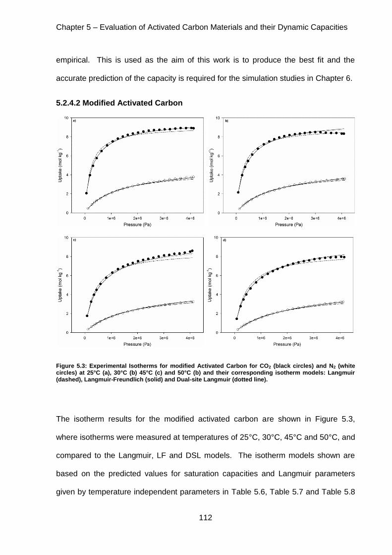
Chapter 5 – Evaluation of Activated Carbon Materials and their Dynamic Capacities
112
empirical. This is used as the aim of this work is to produce the best fit and the
accurate prediction of the capacity is required for the simulation studies in Chapter 6.
5.2.4.2 Modified Activated Carbon
Figure 5.3: Experimental Isotherms for modified Activated Carbon for CO2 (black circles) and N2 (white circles) at 25°C (a), 30°C (b) 45°C (c) and 50°C (b) and their corresponding isotherm models: Langmuir (dashed), Langmuir-Freundlich (solid) and Dual-site Langmuir (dotted line).
The isotherm results for the modified activated carbon are shown in Figure 5.3,
where isotherms were measured at temperatures of 25°C, 30°C, 45°C and 50°C, and
compared to the Langmuir, LF and DSL models. The isotherm models shown are
based on the predicted values for saturation capacities and Langmuir parameters
given by temperature independent parameters in Table 5.6, Table 5.7 and Table 5.8
Chapter 5 – Evaluation of Activated Carbon Materials and their Dynamic Capacities
113
respectively. Similar trends are seen for the modified material as the unmodified
material. The nitrogen isotherm is well matched by all three models used. The
carbon dioxide isotherm is much better described by the LF and DSL models, with
the Langmuir model showing the same over prediction at low pressures and under
prediction at high pressures.
It is possible to compare the isotherms at 30°C and 45°C of the unmodified and
modified activated carbons. At 30°C the unmodified material, Figure 5.2a, actually
shows higher maximum adsorption capacity than the modified material, Figure 5.3b,
with the highest values being 10.0 mol kg-1 and 8.5 mol kg-1 respectively. The
maximum values at 45°C show the reverse trend with the unmodified material, Figure
5.2b, having a maximum of 8.1 mol kg-1 and the modified material, Figure 5.3c, a
maximum of 8.6 mol kg-1. Based on the pore surface area results the modified
material would be expected to have a greater capacity for carbon dioxide, as seen
with the measurements at 45°C. The modified material has maximum capacities
under the conditions studied of 8.92 mol kg-1 at 25°C, 8.56 mol kg-1 at 30°C, 8.61 mol
kg-1 at 45°C and 7.97 mol kg-1 at 50°C, suggesting that there is a much more limited
temperature dependence compared to the unmodified material and that the
saturation capacity is close to being achieved at 4 MPa for all temperatures. The
unmodified material on the other hand sees greater difference between the maximum
value at 30°C and at 45°C, suggesting that temperature has a greater effect on the
capacity and that the saturation capacity has not been reached at 4 MPa at higher
temperatures. This could indicate that the modified material does not have a
significant increase at pressure higher than those studied here and future work is
required to study this.

Chapter 5 – Evaluation of Activated Carbon Materials and their Dynamic Capacities
114
Table 5.6: Langmuir-Freundlich isotherm values for modified activated carbon for N2 and CO2
Parameter N2 CO2
𝐵𝑖,25°𝐶 Pa-n
1.96 x 10⁻⁶ 2.56 x 10
-5
𝐵𝑖,30°𝐶 Pa-n
1.73 x 10⁻⁶ 2.26 x 10
-5
𝐵𝑖,45°𝐶 Pa-n
1.35 x 10⁻⁶ 1.51 x 10
-5
𝐵𝑖,50°𝐶 Pa-n
1.18 x 10⁻⁶ 1.27 x 10
-5
𝑞𝑠,𝑖,25°𝐶 mol kg-1
5.14 10.1 𝑞𝑠,𝑖,30°𝐶 mol kg
-1 5.20 9.92
𝑞𝑠,𝑖,45°𝐶 mol kg-1
5.07 10.1 𝑞𝑠,𝑖,50°𝐶 mol kg
-1 5.37 9.94
𝑛𝑖 - 0.93 0.84 𝑘1,𝑖 mol kg
-1 6.73 10.06
𝑘2,𝑖 J mol-1
670 13.5 𝑘3,𝑖 Pa
-n 3.89 x 10
-9 3.22 x 10
-9
𝑘4,𝑖 J mol-1
-15400 -22300
The LF isotherm parameters are given in Table 5.6. The saturation capacities found
are almost constant at the various temperatures which is in agreement with García et
al. (2013) using a constant value at all temperatures. In order to be consistent with
the unmodified material, a temperature dependence is maintained despite the effect
being minimal for the modified activated carbon. Table 5.7 gives the parameters for
the DSL model for nitrogen upon the modified activated carbon, with similar trends to
the unmodified material observed. The nitrogen parameters include a predicted
saturation capacity that is significantly larger than values typically found in literature,
discussed in Section 5.2.4.1, but, as with the unmodified material, these values give
the best fit to the isotherm data. The carbon dioxide parameters are given in Table
5.8, where the saturation capacities are more consistent with the literature values
discussed in Section 5.2.4.1. Each half the DSL isotherm refers to a particular
adsorption site. The saturation capacity for site 2 is considerably higher than that of

Chapter 5 – Evaluation of Activated Carbon Materials and their Dynamic Capacities
115
site 1, as has been previously seen for activated carbons (García et al., 2013),
suggesting that the majority of adsorption is taking place on this site.
Table 5.7: Dual-site Langmuir isotherm values for modified activated carbon for N2
Parameter N2
25°C 25°C 45°C 50°C
𝐵1,𝑖 Pa-1
1.06 x 10⁻⁶
9.80 x 10⁻⁷
7.85 x 10⁻⁷
7.32 x 10⁻⁷
𝐵2,𝑖 Pa-1
1.04 x 10⁻⁹
1.35 x 10⁻⁹
2.76 x 10⁻⁹
3.45 x 10⁻⁹
𝑞1,𝑠,𝑖 mol kg-1
3.74 3.66 3.42 3.35
𝑞2,𝑠,𝑖 mol kg-1
172 132 62.2 49.2
𝑘1,1,𝑖 mol kg-1
0.90
𝑘1,2,𝑖 J mol-1
3523
𝑘1,3,𝑖 Pa-1
8.91 x 10⁻⁹
𝑘1,4,𝑖 J mol-1
11838
𝑘2,1,𝑖 mol kg-1
1.59 x 10⁻⁵
𝑘2,2,𝑖 J mol-1
40100
𝑘2,3,𝑖 Pa-1
5.51 x 10⁻³
𝑘2,4,𝑖 J mol-1
-38358
Table 5.8: Dual-site Langmuir isotherm values for modified activated carbon for CO2
Parameter CO2
25°C 30°C 45°C 50°C
𝐵1,𝑖 Pa-1
1.17 x 10⁻⁴
7.16 x 10⁻⁵
1.80 x 10⁻⁵
1.17 x 10⁻⁵
𝐵2,𝑖 Pa-1
3.00 x 10⁻⁶
2.48 x 10⁻⁶
1.47 x 10⁻⁶
1.24 x 10⁻⁶
𝑞1,𝑠,𝑖 mol kg-1
0.81 0.91 1.24 1.37
𝑞2,𝑠,𝑖 mol kg-1
8.77 8.61 8.16 8.02
𝑘1,1,𝑖 mol kg-1
737
𝑘1,2,𝑖 J mol-1
-16900
𝑘1,3,𝑖 Pa-1
1.43 x 10⁻¹⁷
𝑘1,4,𝑖 J mol-1
73700
𝑘2,1,𝑖 mol kg-1
2.78
𝑘2,2,𝑖 J mol-1
2850
𝑘2,3,𝑖 Pa-1
3.46 x 10⁻¹¹
𝑘2,4,𝑖 J mol-1
28200

Chapter 5 – Evaluation of Activated Carbon Materials and their Dynamic Capacities
116
5.2.5 Heat of Adsorption
The heat of adsorption can be found using the Clausius-Clapeyron relationship, as
described in Section 4.3. The values are based on the predicted capacity from the
pure component data at each temperature using the LF model. As the Clausius-
Clapeyron relationship is only applicable to regions where there is an ideal bulk gas
phase and a negligible adsorbed phase volume (Pan et al., 1998), the range of
capacities from which the heat of adsorption can be calculated is up to 4 mol kg-1 for
carbon dioxide and 2 mol kg-1 for nitrogen where the heat of adsorption remains
linear for each gas (Gao et al., 2004; Grande et al., 2013; Schell et al., 2012b). The
heats of adsorption at different adsorbed amounts for carbon dioxide are shown in
Figure 5.4a and for nitrogen in Figure 5.4b. The gradient of the plots is influenced by
the changing saturation capacity with temperature for the unmodified material, with a
decrease in saturation capacity at higher temperatures resulting in an increase in
heat capacity with higher adsorbed amounts and vice versa (Do, 1998). The average
values for the carbon dioxide heat of adsorption are 24.7 kJ mol-1 and 26.6 kJ mol-1
for the unmodified and modified activated carbons respectively and for nitrogen are
14.9 kJ mol-1 and 15.7 kJ mol-1. These values are in agreement with literature for
activated carbons which range from 21-30 kJ mol-1 for carbon dioxide and
10-17.5 kJ mol-1 for nitrogen (Agarwal et al., 2010; Chue et al., 1995; Dantas et al.,
2011; Grande et al., 2013; Himeno et al., 2005; Lopes et al., 2011; Salem et al.,
1998; Schell et al., 2012b; Shen et al., 2010).

Chapter 5 – Evaluation of Activated Carbon Materials and their Dynamic Capacities
117
Figure 5.4: Heat of adsorption for the unmodified (black circles) and modified (white triangles) activated carbons for a) CO2 and b) N2
5.3 Breakthrough Rig Calibration
Breakthrough experiments characterise the dynamic response of a given system to a
mixture of carbon dioxide and a less adsorbed gas (i.e. nitrogen or hydrogen), a full
experimental description is given in Section 3.6. The CO2 analyser at the end of the
bed records the fraction of carbon dioxide in the outlet stream. Breakthrough curves
are produced by plotting the output of the CO2 analyser against time. The curves are
recorded from when a flow of carbon dioxide is introduced and mixed with a less
adsorbed component.
It is first necessary to find the dynamic response of the system that surrounds the
fixed bed before it is possible to evaluate the separation that takes place. In order to
gain a full understanding of the system, the response of the CO2 analyser was found
followed by the response of the system without the bed, i.e. the bed removed and the
surrounding pipes connected directly. The system itself will have a certain residence
time and breakthrough which can be recorded by the CO2 analyser. It is necessary
to find the capacity for carbon dioxide in the system in order to accurately find the
dynamic capacity of the material in the fixed bed without the effects of the
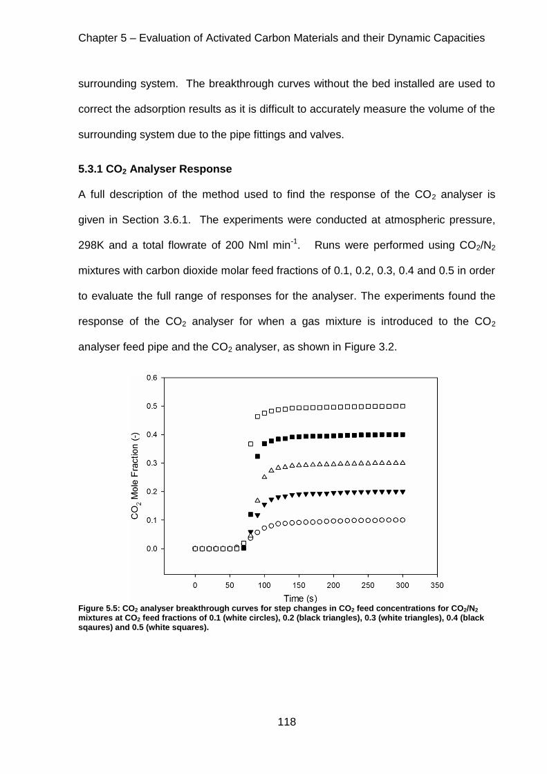
Chapter 5 – Evaluation of Activated Carbon Materials and their Dynamic Capacities
118
surrounding system. The breakthrough curves without the bed installed are used to
correct the adsorption results as it is difficult to accurately measure the volume of the
surrounding system due to the pipe fittings and valves.
5.3.1 CO2 Analyser Response
A full description of the method used to find the response of the CO2 analyser is
given in Section 3.6.1. The experiments were conducted at atmospheric pressure,
298K and a total flowrate of 200 Nml min-1. Runs were performed using CO2/N2
mixtures with carbon dioxide molar feed fractions of 0.1, 0.2, 0.3, 0.4 and 0.5 in order
to evaluate the full range of responses for the analyser. The experiments found the
response of the CO2 analyser for when a gas mixture is introduced to the CO2
analyser feed pipe and the CO2 analyser, as shown in Figure 3.2.
Figure 5.5: CO2 analyser breakthrough curves for step changes in CO2 feed concentrations for CO2/N2 mixtures at CO2 feed fractions of 0.1 (white circles), 0.2 (black triangles), 0.3 (white triangles), 0.4 (black sqaures) and 0.5 (white squares).

Chapter 5 – Evaluation of Activated Carbon Materials and their Dynamic Capacities
119
Figure 5.5 shows the breakthrough curves for the response of the CO2 analyser to a
step change in carbon dioxide for all feed fractions tested. The time for the response
of any step change is consistent across the range of carbon dioxide concentrations
tested. The response times at different fractions of the inlet CO2 fraction for the
breakthrough are given in Table 5.9. The initial breakthrough is relatively consistent,
as are the times for complete breakthrough. The manufacturer gives a t90 response
of 75 seconds, which is lower than all responses found here. There is good
agreement across the range of mole fractions for the initial breakthrough time, t5, and
the time to reach complete saturation, t100, suggesting that the analyser responds in
the same way at all concentrations. The time taken from breakthrough to reach
complete saturation is considerably longer than the initial breakthrough time, with the
majority of this being in the last 0.01 mole fraction of the absolute reading as seen in
the final column in Table 5.9. Therefore, it is important that this delay for the final
aspects of the carbon dioxide concentration is attributed to the response of the
measurement device.
Table 5.9: Response times for the CO2 analyser at various feed concentrations given at percentages of the feed concentration
CO2 Feed Fraction
Response Time t5 (s) t90 (s) t100 (s) t0.01,mf (s)
0.1 62 139 264 139 0.2 68 119 259 150 0.3 76 107 259 134 0.4 75 97 267 140 0.5 71 87 280 136
5.3.2 System Characterisation
Breakthrough curves were produced for an experimental set up with the fixed bed
removed and the inlet and outlet pipes connected directly, as shown in Figure 3.7. A

Chapter 5 – Evaluation of Activated Carbon Materials and their Dynamic Capacities
120
full description of the experimental procedure is given in Section 3.7.2. The
experiment was performed for both CO2/N2 mixtures and CO2/H2 mixtures to find the
carbon dioxide captured by the system for both gas mixtures. All experiments were
conducted at 2.5 MPa, 298K and a total flowrate of 200 Nml min-1.
5.3.2.1 CO2/N2 System Response
Figure 5.6: Breakthrough curves for a system without a bed when step changes in CO2 feed concentrations for CO2/N2 mixtures are introduced at CO2 feed fractions of 0.1 (white circles), 0.2 (black triangles), 0.3 (white triangles), 0.4 (black sqaures) and 0.5 (white squares).
The breakthrough curves for the system without the packed bed and the pipe
connections linked directly are shown in Figure 5.6 and the corresponding response
times are shown in Table 5.10 for a CO2/N2 mixture. The system does not respond
as a perfect plug flow system with the same breakthrough time for all feed fractions
of carbon dioxide. This is caused by dispersion in a section of pipe between the
mass flow controller regulating the flow of carbon dioxide and the junction where the

Chapter 5 – Evaluation of Activated Carbon Materials and their Dynamic Capacities
121
nitrogen and carbon dioxide mix. The residence time for the carbon dioxide in this
pipe varies for each run as the overall flowrate is kept constant, meaning the carbon
dioxide flowrate is varied to achieve this. The system shows a similar trend to the
CO2 analyser result, with considerably longer times between the t50t100 than for the
t5t50. This will be partly due to the response of the analyser, discussed in Section
5.3.1, but will also be due to some dispersion in the general system leading to a
spreading of the breakthrough curve. The amount of carbon dioxide that remains in
the system for each feed fraction is also given in Table 5.10. It can be seen that
there is a constant increase of 5.1 x 10⁻³ mol for each increase of 0.1 in feed mole
fraction. The carbon dioxide in the pipe between the CO2 control valve and the
mixing junction is given by the intercept of a straight line plot, shown in Appendix I,
between the amount of carbon dioxide accumulated and the CO2 feed fraction, with a
value of 4.7 x 10⁻³ mol. The total value for carbon dioxide accumulated in the
system, as given in Table 5.10, can be subtracted from the total capacity found for
the fixed bed adsorption systems to give the amount of carbon dioxide captured by
the fixed bed.
Table 5.10: Response times for the system without a bed at various feed concentrations of a CO2/N2 given at percentages of the feed concentration
CO2 Feed Fraction
Response Time CO2 Captured
(mol) t5 (s) t50 (s) t100 (s)
0.1 530 619 1300 1.00 x 10⁻²
0.2 414 467 1148 1.52 x 10⁻² 0.3 358 396 1066 1.99 x 10⁻² 0.4 338 364 1108 2.51 x 10⁻² 0.5 327 344 1173 3.09 x 10⁻²

Chapter 5 – Evaluation of Activated Carbon Materials and their Dynamic Capacities
122
5.3.2.2 CO2/H2 System Response
The breakthrough results for a CO2/H2 mixture passed through a system without a
bed are shown in Figure 5.7. The breakthrough times and accumulated carbon
dioxide in the surrounding pipes and valves are given in Table 5.11, showing very
similar results to those given by CO2/N2 mixtures. Based on the capacity results, the
system without a bed shows an increase in accumulated carbon dioxide of
4.4 x 10⁻³ mol for each carbon dioxide feed fraction increase of 0.1. The amount of
carbon dioxide accumulated in the pipe leading to the mixing junction was
5.6 x 10⁻³ mol, based on the plot of the CO2 feed fraction versus the accumulated
carbon dioxide as done for the CO2/N2 mixture. These values for the accumulated
carbon dioxide in the surrounding pipes and fittings for the fixed bed measurements
using CO2/H2 mixtures can be subtracted from the readings with the bed installed, so
that the carbon dioxide capacity for the breakthrough experiments with the bed
included will be more accurate.
Figure 5.7: Breakthrough curves for a system without a bed when step changes in CO2 feed concentrations for CO2/H2 mixtures are introduced at CO2 feed fractions of 0.1 (white circles), 0.2 (black triangles), 0.3 (white triangles), 0.4 (black sqaures) and 0.5 (white squares).

Chapter 5 – Evaluation of Activated Carbon Materials and their Dynamic Capacities
123
Table 5.11: Response times for the system without a bed at various feed concentrations of a CO2/H2 mixture given at percentages of the feed concentration
CO2 Feed Fraction
Response Time CO2 Captured
(mol) t5 (s) t50 (s) t90 (s) t100 (s)
0.1 549 648 855 1150 1.02 x 10⁻²
0.2 393 448 562 797 1.43 x 10⁻² 0.3 341 377 480 803 1.84 x 10⁻² 0.4 325 353 447 867 2.35 x 10⁻² 0.5 308 328 407 785 2.78 x 10⁻²
5.4 Activated Carbon Breakthrough Experiments
Breakthrough curves for separation of CO2/N2 mixtures using unmodified activated
carbon were conducted as described in Section 3.7.2. The experimental conditions
are given in Table 5.12.
Table 5.12: Experimental conditions for separations using the unmodified activated carbon
Bed Length m 0.069 Bed Diameter m 0.025 Adsorption Pressure
MPa 2.5
Temperature K 298 Feed Flowrate Nml min-1 200 Adsorbent Mass g 8.88
5.4.1 Experimental Breakthrough Curves
Figure 5.8 shows the response of the CO2 analyser to a step change in carbon
dioxide in the feed stream for the whole experimental set-up to give the carbon
dioxide breakthrough curves at varying carbon dioxide feed mole fractions for the
unmodified activated carbon. As the response of the system without a bed is not a
simple time delay, as shown in Section 5.3.2, it is not possible to remove the effect
on the breakthrough curve. This is instead evaluated in the adsorption capacity see
Section 5.4.2. The results are shown at 100 s intervals so as to distinguish the

Chapter 5 – Evaluation of Activated Carbon Materials and their Dynamic Capacities
124
individual points. The breakthrough time is found by taking the time at which the
outlet CO2 fraction reaches 5% of the inlet CO2 fraction. As the feed mole fraction
increases, a proportional drop in breakthrough time would be expected if the capacity
was constant. However, the breakthrough times do not decrease proportionally with
the increase in carbon dioxide concentration, showing higher adsorption capacities at
higher CO2 feed fractions. This is consistent with the isotherm data where at higher
pressures of carbon dioxide a larger amount of carbon dioxide is adsorbed.
Figure 5.8: Breakthrough curves for the separation of a CO2/N2 mixture using unmodified activated carbon at CO2 feed fractions of 0.1 (black circles), 0.2 (white squares), 0.3 (black triangles), 0.4 (white triangles) and 0.5 (black diamonds)
The shape of the breakthrough curve gives strong indications of the dispersion
characteristics and mass transfer limitations of the system. Systems with large
dispersion or mass transfer resistances have long shallow breakthrough curves
(Ruthven, 1984). Garg and Ruthven (1975) suggest the effect both the mass transfer
coefficient and the dispersion coefficient is additive but there is no way to attribute
the cause of the steepness of the breakthrough curve to one effect or the other. The
steepness of the curves in Figure 5.8 indicates that this effect is relatively small in the

Chapter 5 – Evaluation of Activated Carbon Materials and their Dynamic Capacities
125
work reported here, i.e. neither coefficient is significantly affecting the breakthrough
curve. The breakthrough for a CO2 feed fraction of 0.1 displays the greatest amount
of spreading. This is to be expected as the residence time is the longest. The error
on this reading will also be the highest and the mole fraction recorded by the CO2
analyser has an absolute error of ± 0.01, leading to a 10% error on the 0.1 run. It is
suggested by Garcia et al. (2011) that higher pressures lead to greater spreading
due to higher degrees of dispersion, but it is not clear if this is attributed to higher
absolute pressures or carbon dioxide partial pressures. This work shows that higher
partial pressures with a fixed absolute pressure give less mass transfer and
dispersion limitations.
Table 5.13: The overall mass transfer coefficient as well as the contribution of each mass transfer resistance for a system with a CO2 feed fraction of 0.4
CO2 N2
Overall Mass Transfer Coefficient
s-1 0.099 0.815
Film Mass Transfer s-1 0.67 8.60
Pore Mass Transfer s-1 0.43 5.47
Micropore Mass Transfer s-1 0.16 1.08
It is possible to quantify the dispersion and mass transfer effects by using
correlations that are given in Section 4.7. The Hsu and Haynes (1981) correlation is
shown in Section 6.3.2.2 to be the most suitable for the experiments here and this
predicts a dispersion coefficient of 1.5 x 10⁻⁶ m2 s-1. The mass transfer correlation
suggested by Farooq and Ruthven (1990) combines all three mass transfer modes
without the need for individual equations for each mass transfer mode and is used in
the simulation of the breakthrough curves in Section 6.3.2. It is possible to calculate
the degree to which each mass transfer resistance affects the overall mass transfer

Chapter 5 – Evaluation of Activated Carbon Materials and their Dynamic Capacities
126
resistance by calculating the individual parts of Equation 4.39, the results are
presented in Table 5.13. These results show that all three resistances impact the
overall mass transfer but the micropore resistance is the most significant. This
disagrees with Farooq and Ruthven (1990), who find the micropore resistance
negligible, although this was found for zeolite 5A. Shen et al. (2010) show that
micropore resistance for activated carbon using carbon dioxide and nitrogen controls
the diffusion mechanism, which agrees with the micropore mass transfer resistance
being the most significant. The total mass transfer coefficient agrees with the
experimental results found by Casas et al. (2012), who found a carbon dioxide and
hydrogen mass transfer coefficient of 0.15 s-1 and 1.0 s-1 respectively. The values for
the dispersion and mass transfer coefficients confirm that the system is not
significantly affected by either effect leading to the steep breakthrough curves shown
in Figure 5.8.
Figure 5.9: Temperature profile for the separation using a CO2 feed fraction of 0.1
Figure 5.9 shows the experimentally measured temperature at the bed exit for the
adsorption at a CO2 feed fraction of 0.1, with similar temperature profiles (not shown)

Chapter 5 – Evaluation of Activated Carbon Materials and their Dynamic Capacities
127
for all other CO2 feed fractions. It should be noted that due to the Swagelok fittings
required the thermocouple was located slightly downstream of the bed and any
possible rise in temperature in the bed might not have been detected due to the
cooling of gas as it flowed out of the bed. It is clear from Figure 9 that there is no
significant detectable temperature change at the bed exit which differs from literature,
with Casas et al. (2012) reporting increases of up to 40°C. The breakthrough curve
itself suggests that there is an internal temperature change. A temperature increase
in the bed would not reduce the overall capacity as the adsorbent capacity would
increase as the bed cools, instead a broadening of the breakthrough curve would be
observed (Ruthven et al., 1975). The curves in Figure 5.8 are asymmetric, with the
second part of each of the curves much broader than the initial, similar to the results
seen by Lopes et al. (2009) and by Casas et al. (2012). The temperature front often
moves at a different velocity to the mass transfer front leading to an asymmetric
breakthrough curve, suggesting there is a temperature change taking place and the
broader top half of the curve indicates a lagging temperature profile (Ruthven et al.,
1975). The steepness of the breakthrough curves and absence of temperature
change at the bed exit suggests that any temperature changes are being dissipated
very quickly. The distance between the temperature probe and the bed exit would
give further chance for the gas to cool. The work by Ruthven et al. (1975) show
theoretically that the steepness of the breakthrough curve is associated with the heat
transfer rates out of the bed, with high heat transfer values leading to steep
breakthrough curves as observed in Figure 5.8. A high heat transfer coefficient
would be consistent with there being no significant temperature change detected at
the bed exit. These two factors suggest that there is most likely an internal

Chapter 5 – Evaluation of Activated Carbon Materials and their Dynamic Capacities
128
temperature change in the bed but that the heat is rapidly dissipated before the gas
reaches the temperature probe.
5.4.2 Breakthrough CO2 Capacity
The dynamic capacity of the bed is considered based on the breakthrough capacity
rather than the total saturation capacity. A PSA system would not be run until
complete saturation of the bed and therefore a breakthrough capacity is a more
realistic prediction of the working capacity of a process unit. This is found by
assuming that all carbon dioxide input to the system up until the breakthrough time is
captured by the system. The system capacities found for the experimental setup
without a bed, given in Table 5.10, were subtracted to give the capacity of the bed
only. The carbon dioxide that occupies the void space in the bed is also deducted to
give the amount of carbon dioxide that is in the adsorbed phase. The average
capacity over three cycles is given for each feed fraction in Table 5.14. The capacity
found by the experimental set up would be expected to be higher than that of a PSA
unit as the bed is fully cleaned between each run. The results show that the increase
in breakthrough capacity is larger between lower feed fractions than the highest feed
fractions. This is in agreement with the isotherm data, shown in Figure 5.2, where an
increase in pressure at lower values has a greater increase in capacity than it does at
higher pressures. Table 5.14 also gives the predicted values for the carbon dioxide
capacity for pure component data at the equivalent partial pressure. The isotherm
gives a value for equilibrium conditions and it is also for pure component data, i.e.
assuming that the nitrogen in the mixture does not interact or compete with carbon
dioxide. Both of these factors explain the large disparity between the values. The
greater difference between the breakthrough capacity and the predicted isotherm

Chapter 5 – Evaluation of Activated Carbon Materials and their Dynamic Capacities
129
value for a feed fraction of 0.1 further emphasises the larger degree of spreading in
the breakthrough curve at the lower feed fractions, and the further the system from
equilibrium. The almost constant difference for all other values suggests the mass
transfer front is well established for all those runs.
It is important to find an isotherm model which can accurately represent the
experimental data. The large difference between the isotherm models and the
breakthrough data suggest that the presence of nitrogen has a significant impact on
the carbon dioxide capacity and models capable of replicating this are required. It is
easier to produce pure component isotherm data rather than multicomponent data.
As discussed in Section 4.2, there are several models that use pure component data
to predict multicomponent adsorption capacities. Due to the strong agreement for
the pure component isotherms shown in Section 5.2.4.1, the multicomponent
Langmuir-Freundlich (LF) model and multicomponent dual site Langmuir (DSL)
model were used to predict the carbon dioxide capacity. For each of these models,
the Ideal Adsorbed Solution Theory (IAST) was also applied to their corresponding
pure component results, with the theory behind this discussed in Section 4.2.2.
Table 5.14: The breakthrough capacities of CO2/N2 mixtures separated using unmodified activated carbon for each experimental run and the predicted capacity for pure components based on the LF and DSL models
CO2 Feed
Fraction Breakthrough
Capacity LF Model DSL Model
(-) (mol kg-1
) (mol kg-1
) (mol kg-1
) 0.1 2.12 ± 0.14 4.38 4.43 0.2 4.05 ± 0.15 5.93 5.94 0.3 5.01 ± 0.08 6.88 6.86 0.4 5.54 ± 0.17 7.55 7.51 0.5 6.09 ± 0.06 8.06 8.02

Chapter 5 – Evaluation of Activated Carbon Materials and their Dynamic Capacities
130
Table 5.15 compares the predicted capacity for both carbon dioxide and nitrogen by
the multicomponent LF, the IAST LF, the multicomponent DSL and the IAST DSL. It
can be seen that the various models differ in their prediction of the carbon dioxide
capacity. The IAST LF predicts a higher capacity for carbon dioxide than the
multicomponent LF and a lower capacity for nitrogen. The IAST model also predicts
a much higher selectivity for carbon dioxide, especially at higher carbon dioxide
partial pressures. Both models show considerably higher capacities than the
breakthrough capacities. The comparisons in literature have been to experimental
multicomponent isotherms, where the IAST model has been shown to have similar
prediction capabilities as multicomponent models (Dreisbach et al., 1999; Rother and
Fieback, 2013; Schell et al., 2012b).
Table 5.15: Predicted multicomponent adsorption capacities based on the multicomponent LF and DSL models and the corresponding IAST models for CO2/N2 mixtures separated using unmodified activated carbon
CO2
Feed Fraction
CO2
Breakthrough Capacity
IAST – LF Model
LF Model IAST – DSL
Model DSL Model
(mol kg-1
) (mol kg-1
) (mol kg-1
) (mol kg-1
)
(-) (mol kg-1
) CO2 N2 CO2 N2 CO2 N2 CO2 N2
0.1 2.12 ± 0.14 2.80 0.94 2.88 2.04 2.55 1.11 2.95 1.97 0.2 4.05 ± 0.15 4.49 0.60 4.27 1.66 3.88 0.79 4.75 1.43 0.3 5.01 ± 0.08 5.70 0.40 5.30 1.37 4.82 0.60 5.99 1.06 0.4 5.54 ± 0.17 6.60 0.27 6.12 1.13 5.58 0.46 6.91 0.79 0.5 6.09 ± 0.06 7.30 0.18 6.82 0.91 6.21 0.35 7.62 0.59
The DSL models show the opposite trend with the IAST-DSL model predicting lower
carbon dioxide and nitrogen capacities than the multicomponent DSL model. The
difference may lie in the way that the multicomponent system predicts the capacity.
As there are two sites, the way the two component isotherms interact can vary and
results here are all assumed to be for a positive-positive system, as discussed in

Chapter 5 – Evaluation of Activated Carbon Materials and their Dynamic Capacities
131
Appendix A, but the IAST model is unable to take this into account. Reversing the
interaction of the DSL sites results in a dramatically lower prediction in capacity and
therefore that model has been discounted. The IAST model under predicts the
breakthrough capacity, with the values for feed fraction of 0.3 and 0.4 actually being
lower than the breakthrough capacity. This is because the IAST model is unable to
take the interaction of the sites into account. The application of the DSL is limited in
literature and the application to the IAST model even more so. It has previously been
applied to the IAST model for activated carbons by Dreisbach et al. (1999), however,
a Freundlich type exponent was included as well. The IAST does not always provide
a better fit to multicomponent data (Schell et al., 2012b) and in this case the data in
Table 5.15 indicates that the IAST model under predicts the breakthrough capacity,
with the multicomponent DSL a better fit.
For both models, the solution method which predicts the higher capacity is more
likely to be accurate. There is still an appreciable degree of spreading shown in
Figure 5.8 which would suggest that the breakthrough capacity should still be
significantly lower than an equilibrium capacity. On this basis, the IAST LF and the
multicomponent DSL models are more suitable.
5.5 Modified Activated Carbon Breakthrough Experiments
The experimental set up for the modified material is the same as the unmodified
material and is described in detail in Section 3.7.2. The key experimental conditions
are given in Table 5.16.

Chapter 5 – Evaluation of Activated Carbon Materials and their Dynamic Capacities
132
Table 5.16: Experimental conditions for separations using the modified activated carbon
Bed Length m 0.065 Bed Diameter m 0.025 Adsorption Pressure
MPa 2.5
Temperature K 298 Feed Flowrate Nml min-1 200 Adsorbent Mass g 6.11
5.5.1 CO2/N2 Separations
5.5.1.1 Breakthrough Curves and Capacities
The breakthrough curves for the modified activated carbon are shown in Figure 5.10
alongside the breakthrough curves for the unmodified material. As for the unmodified
activated carbon in Section 5.4.1, the steepness of the curves show there is still very
limited mass transfer and dispersion effects. From the correlations discussed in
Section 5.4.1, the dispersion coefficient here was found to be 1.86 x 10⁻⁶ m2 s-1 and
the mass transfer coefficients to be 0.07 s-1 and 0.99 s-1 for the carbon dioxide and
nitrogen respectively. These values suggest that dispersion and mass transfer
limitations have only a slightly larger effect than for the unmodified material. The
breakthrough times are slightly shorter for the modified material. This is mainly due
to there being significantly less adsorbent, on a mass basis, in the bed. The
difference in density means that the fixed bed for the modified material is almost 33%
lighter. The capacity would actually be expected to be less than found here
considering the large difference in bed density with only a slight increase in capacity
shown by the isotherms.

Chapter 5 – Evaluation of Activated Carbon Materials and their Dynamic Capacities
133
Figure 5.10: Breakthrough curves for the separation of a CO2/N2 mixture using unmodified activated (black) compared with the modified activated carbon material (white).
The breakthrough capacity for each run is given in Table 5.17 as well as a
comparison to the pure component capacity as predicted by the LF and DSL models.
At lower feed fractions the difference between the breakthrough capacity and the
equilibrium capacity from the isotherm is considerable but this reduces as the carbon
dioxide feed fraction increases. As the material has not reached saturation at
breakthrough, the small differences between the isotherm prediction and the
breakthrough capacity at higher feed fractions can be mainly attributed to the
material not being at equilibrium. This suggests that the higher concentration of
carbon dioxide and better selectivity mean the majority of the adsorption sites are
occupied by carbon dioxide and the interaction by the nitrogen is limited allowing the
carbon dioxide capacity to approach that of a pure component.

Chapter 5 – Evaluation of Activated Carbon Materials and their Dynamic Capacities
134
Table 5.17: The breakthrough capacities of CO2/N2 mixtures separated using modified activated carbon for each experimental run and the predicted capacity for pure components based on the LF and DSL models.
CO2 Feed
Fraction Breakthrough
Capacity LF DSL
(-) (mol kg-1
) (mol kg-1
) (mol kg-1
) 0.1 2.61 ± 0.13 4.61 4.53 0.2 4.67 ± 0.04 6.05 6.07 0.3 5.88 ± 0.14 6.83 6.88 0.4 6.84 ± 0.16 7.32 7.39 0.5 7.48 ± 0.09 7.68 7.74
Table 5.18: Predicted multicomponent adsorption capacities based on the multicomponent LF and DSL models and the corresponding IAST models for CO2/N2 mixtures separated using modified activated carbon
CO2
Feed Fraction
CO2 Breakthrough
Capacity
IAST – LF Model
LF Model IAST – DSL
Model DSL Model
(mol kg-1
) (mol kg-1
) (mol kg-1
) (mol kg-1
)
(-) (mol kg-1
) CO2 N2 CO2 N2 CO2 N2 CO2 N2
0.1 2.61 ± 0.13 2.74 1.24 2.58 2.27 2.74 1.21 4.48 0.50 0.2 4.67 ± 0.04 4.46 0.77 3.98 1.76 4.38 0.80 6.02 0.27 0.3 5.88 ± 0.14 5.62 0.49 4.98 1.39 5.45 0.57 6.85 0.17 0.4 6.84 ± 0.16 6.43 0.32 5.77 1.09 6.19 0.41 7.37 0.12 0.5 7.48 ± 0.09 7.01 0.21 6.40 0.85 6.73 0.30 7.72 0.08
A similar comparison is made in Table 5.18 between the multicomponent models for
predicting the capacity of the material for each gas and the experimental
breakthrough capacities. The same trend is seen as for the unmodified material, with
the multicomponent LF and the IAST DSL predicting lower carbon dioxide capacities
than their counterparts. In these cases the two IAST models also predict similar
carbon dioxide capacities for all feed fractions. However, the IAST models and the
multicomponent LF model under predict the breakthrough capacity at higher feed
fractions. The multicomponent DSL model is the only one that predicts a greater
equilibrium capacity than the breakthrough capacity for all feed fractions. This is
because the predicted nitrogen interaction is the least and therefore the predicted

Chapter 5 – Evaluation of Activated Carbon Materials and their Dynamic Capacities
135
carbon dioxide capacities are very similar to the pure component equilibrium
prediction. As the breakthrough capacity results suggest very limited interaction with
the nitrogen, this model most suitably represents the system.
5.5.1.2 Capacity Comparison to Unmodified Activated Carbon
Figure 5.11: Comparison of unmodified (black circles) and modified (white circles) activated carbon breakthrough capacities for the separation of CO2/N2 mixtures on a a) mass and b) volumetric basis
A comparison can be performed between the breakthrough capacities for each
material. In Section 5.2.4, the isotherms show that the unmodified material has
slightly greater equilibrium capacities than the modified material. Figure 5.11a
compares the breakthrough capacities of the material on the same mass basis. The
modified material outperforms the unmodified activated carbon for all feed fractions,
with the greatest difference at higher feed fractions. It is apparent that the selectivity
for carbon dioxide over nitrogen is greater for the modified material as the
breakthrough capacities are much closer to the pure component equilibrium value.
This effect is more apparent at higher carbon dioxide partial pressures, which might
explain the greater difference in breakthrough capacity between the two values at
higher feed fractions.

Chapter 5 – Evaluation of Activated Carbon Materials and their Dynamic Capacities
136
Although the carbon dioxide capacity on a mass basis is often quoted for materials, it
is actually the capacity on a volumetric basis that is more important for a PSA
process. Section 5.2.3 shows that the unmodified material has a higher bulk density
than the modified material, meaning a higher mass of material fits in the same bed
volume. The number of moles of carbon dioxide captured per meter cubed of bed
can be found by multiplying the mass capacity by the bulk density of the bed. The
results of this upon the carbon dioxide capacity per unit volume are shown in Figure
5.11b, with the unmodified material greatly outperforming the modified material. This
is to be expected as the bulk density is considerably larger for the unmodified
material with only a slight decrease in equilibrium capacity found by the isotherm.
This emphasises the importance of finding the carbon dioxide capacity on a
volumetric basis. Drage et al. (2009a) indicate this in their evaluation of materials for
pre-combustion capture. However, literature values for dynamic capacities are rarely
quoted and often on a mass basis for comparison to equilibrium values found from
isotherms (García et al., 2011). The work by Martin et al. (2012) briefly comments on
this but the materials being compared show a very limited difference in density and
therefore in their volumetric capacity. Capacities being quoted on a mass basis
instead of a volumetric basis when found from isotherms also calls into question
observations that capacity increases for materials with greater pore surface area
(Drage et al., 2009a; Sun et al., 2013). This is true on a mass basis but often this
greater pore surface area results in a lower density as there needs to be greater pore
structures to give the higher pore surface area. An increase in pore surface area is
often the focus of modification to activated carbons, however, may not have an effect
on the volumetric capacity and therefore the capacity of a fixed bed PSA unit.

Chapter 5 – Evaluation of Activated Carbon Materials and their Dynamic Capacities
137
5.5.2 CO2/H2 Separations
Figure 5.12: Breakthrough curves for the separation of a CO2/H2 mixture using modified activated carbon at CO2 feed fractions of 0.1 (black circles), 0.2 (white squares), 0.3 (black triangles), 0.4 (white triangles) and 0.5 (black diamonds)
For the development of PSA processes for the separation of carbon dioxide at high
pressures, it is important to consider a CO2/H2 mixture to ensure the results of a
simulation using CO2/N2 would give reasonable indications for applications towards
CO2/H2 mixtures. Therefore, the fixed bed experiments were repeated for the
modified activated carbon using a CO2/H2 gas mixture. The breakthrough curves,
given in Figure 5.12, show that there is a much greater degree of spreading than for
the CO2/N2 mixture separations. It is possible to predict the mass transfer and
dispersion coefficients by correlations as done in Section 5.4.1. For the CO2/N2
system, the rate limiting step for mass transfer was into the micropores. These are
highly system specific and require complex experiments to find which was outside
the scope of this work. However, as a different micropore diffusion would only affect

Chapter 5 – Evaluation of Activated Carbon Materials and their Dynamic Capacities
138
the hydrogen mass transfer coefficient, there is no reason for the carbon dioxide
mass transfer coefficient to be affected by the use of hydrogen instead of nitrogen
and therefore is likely to be constant for the system. The surface and macropore
mass transfer resistances are calculated using isotherm data. As a first
approximation, it can be assumed that no hydrogen is adsorbed and this gave a
carbon dioxide mass transfer coefficient of 0.156 s-1 and a hydrogen mass transfer
coefficient of 1.08 s-1. These are slightly larger than the mass transfer coefficients for
the CO2/N2 system and would therefore not lead to the larger degree of spreading.
The other coefficient that strongly affects the shape of the breakthrough curve is the
dispersion coefficient, calculated from the Peclet number. The main properties that
affect this are the density, viscosity and the diffusivity of the gas mixture. However,
the Peclet number is a product of the Reynolds and Schmidt number which cause the
viscosity and density effects to cancel out, making it only reliant on the mixture
diffusivity. For a CO2/H2 mixture the calculated diffusivity increases (Bird et al.,
2001). This gives a decrease in the Reynolds and Schmidt number product for the
CO2/H2 mixture compared to the CO2/N2 mixture, as shown in Appendix J. For the
Hsu and Haynes (1981) correlation the dispersion coefficient can be calculated to
give a value of 1.62 x 10⁻⁶ m2 s-1 for CO2/H2 mixtures compared to 1.86 x 10⁻⁶ m2 s-1
for CO2/N2 mixtures over the modified activated carbon. This does not explain the
greater degree of spreading for the CO2/H2 breakthrough curves shown in Figure
5.12. It is most likely that a different dispersion coefficient correlation, where the
dispersion coefficient is predicted to be larger for CO2/H2 mixtures, see Appendix J, is
required for these mixtures.

Chapter 5 – Evaluation of Activated Carbon Materials and their Dynamic Capacities
139
Table 5.19: The breakthrough capacities of CO2/H2 mixtures separated using modified activated carbon for each experimental run and the predicted capacity for pure components based on the LF and DSL models
CO2 Feed
Fraction Breakthrough
Capacity LF Model DSL Model
(-) (mol kg-1
) (mol kg-1
) (mol kg-1
) 0.1 4.32 ± 0.08 4.61 4.53 0.2 5.72 ± 0.01 6.05 6.07 0.3 6.62 ± 0.02 6.83 6.88 0.4 7.34 ± 0.01 7.32 7.39 0.5 7.67 ± 0.04 7.68 7.74
The breakthrough capacities for the CO2/H2 separations are given in Table 5.19. The
closeness of the breakthrough capacity to the pure component equilibrium capacity
suggests that the hydrogen has a limited effect on the capacity for carbon dioxide.
The selectivity is greatest at higher feed fractions where the breakthrough capacity is
almost at parity with the equilibrium capacity. In literature, it has been shown that the
hydrogen capacity on activated carbon is considerably lower than nitrogen (García et
al., 2013; Lopes et al., 2009; Martín et al., 2012; Schell et al., 2012b; Siriwardane et
al., 2001). This low capacity suggests hydrogen in the gas mixture has very little
impact on the capacity for carbon dioxide. It is not possible to calculate the
multicomponent predictions by the isotherm models as equipment limitations meant
the hydrogen isotherm was not found.
By comparing these to values given for CO2/N2 separations in Table 5.17, it is clear
that the carbon dioxide capacity for CO2/H2 mixtures is greater than for CO2/N2
mixtures. However, at the higher feed fractions the difference is minimal. This
suggests that for both separations, the weakly adsorbed component has less of an
effect as the carbon dioxide partial pressure increases. The selectivity for carbon
dioxide over hydrogen is high for all runs but is also high for CO2/N2 mixtures when

Chapter 5 – Evaluation of Activated Carbon Materials and their Dynamic Capacities
140
carbon dioxide feed fractions increases. This limited difference in capacity for
CO2/N2 mixtures and CO2/H2 mixtures at higher feed fractions is promising for
validation of a computer model using a CO2/N2 mixture as pre-combustion application
of a PSA system would also have high fractions of carbon dioxide present.
5.6 Cyclic Experiments
The experimental set up has been used to investigate aspects of a PSA cycle. Both
3 step and 4 step cycles, as described in detail in Section 3.7, were investigated to
study the selectivity of the materials for carbon dioxide over the less adsorbed gas,
nitrogen.
5.6.1 Three step cycle
The 3 step cycle consists of an adsorption step, a joint depressurisation and purge
step, and a pressurisation step. The outlet carbon dioxide feed fraction for the first 2
steps for a separation for a CO2/N2 mixture with 40% carbon dioxide using
unmodified activated carbon is given in Figure 5.13 and is typical of 3 step cycles for
both materials at all feed fractions. As the bed is run to complete saturation, the
adsorption step gives the same results as Figure 5.8. The depressurisation and
purge step initially displays a large spike in the fraction of carbon dioxide. This is
because the adsorbent material releases the adsorbed gases when the pressure of
the system is decreased. As there is more carbon dioxide adsorbed than nitrogen,
the fraction of carbon dioxide increases. After depressurising the bed, the fraction of
carbon dioxide rapidly decreases as the released carbon dioxide is driven away by
the supply of pure nitrogen.

Chapter 5 – Evaluation of Activated Carbon Materials and their Dynamic Capacities
141
Figure 5.13: CO2 exit fraction for the separation of a CO2/N2 mixture using unmodified activated carbon at a CO2 feed fraction of 0.4 followed by a depressurisation and purge under a pure nitrogen flow
The peak of the depressurisation curve gives an indication of the amount of carbon
dioxide in the adsorbed phase. It does not give the actual selectivity due to the
nitrogen purge gas mixing with the released carbon dioxide but does give a
qualitative guide. The peak values for various mole fractions for both the unmodified
material and modified material are given in Table 5.20. The error on the peak values
is generally within the experimental error for the analyser of ± 0.01. Greater error is
possible as the analyser required calibration which was set to the carbon dioxide
mole feed fraction as this was controlled. For all three experimental sets there is a
considerable increase between feed fractions of 0.1 and 0.2. The CO2/N2 mixtures
then display a further step up when the feed fraction is increased to 0.3. All
remaining feed fractions then give relatively consistent peak values. This
emphasises that the nitrogen plays a significant role in the separation at lower carbon
dioxide partial pressures but this is greatly reduced at the highest carbon dioxide

Chapter 5 – Evaluation of Activated Carbon Materials and their Dynamic Capacities
142
feed fractions. This mimics the comparison of the breakthrough capacities with the
carbon dioxide pure component isotherm predictions given in Sections 5.4.2, 5.5.1
and 5.5.2, where the difference is much less at higher feed fractions of carbon
dioxide. The CO2/H2 separation using the modified material reaches higher
selectivity at lower feed fractions due to the low amount of hydrogen adsorbed by
activated carbons as described in Section 5.5.2, meaning it reaches a consistent
level of exit fraction, with the hydrogen having limited interaction effects, at lower
partial pressures of carbon dioxide.
Table 5.20: Average peak desorption exit fractions for the unmodified and modified materials using CO2/N2 and CO2/H2 mixtures
CO2 Feed Fraction (-)
Peak Desorption Exit CO2 Fraction (-) AC – CO2/N2 MAC – CO2/N2 MAC – CO2/H2
0.1 0.57 ± 0.009 0.51 ± 0.015 0.65 ± 0.012 0.2 0.69 ± 0.003 0.63 ± 0.006 0.71 ± 0.018 0.3 0.75 ± 0.009 0.70 ± 0.003 0.70 ± 0.007 0.4 0.77 ± 0.006 0.71 ± 0.029 0.73 ± 0.004 0.5 0.78 ± 0.006 0.74 ± 0.008 0.75 ± 0.016
5.6.2 Four step cycle
As discussed in Section 2.8, a typical PSA cycle is four steps, requiring an adsorption
step, a blowdown step, a purge step and a pressurisation step. The system was run
with the unmodified and modified activated carbon in the bed for the separation of
CO2/N2 mixtures. The adsorption step used a CO2 feed fraction of 0.4 and lasted for
1510 s for the unmodified material and 1260 s for the modified material based on the
breakthrough time found in Sections 5.4.1 and 5.5.1.1 respectively. The CO2 mole
fraction at the exit of the bed for these first three steps for a bed packed with the
unmodified activated carbon is given in Figure 5.14. The cycle shown is typical for
the modified activated carbon as well. The adsorption step shows that after 1510 s

Chapter 5 – Evaluation of Activated Carbon Materials and their Dynamic Capacities
143
there is a small amount of carbon dioxide in the outlet stream. During the blowdown
step, the rapid pressure change causes the carbon dioxide fraction to rise rapidly.
The remaining part of the blowdown step allows the system to equilibrate so that the
outlet fraction recorded by the analyser is the same as that in the bed. The purge
step is then similar to that of the 3 step cycle, with the carbon dioxide exit fraction
decreasing rapidly as the nitrogen flow flushes it out of the system.
Figure 5.14: CO2 exit fraction for the separation of a CO2/N2 mixture using unmodified activated carbon at a CO2 feed fraction of 0.4 for 1510 s followed by a depressurisation with no flow for 600 s and then purge under a pure nitrogen flow for 2100 s. Results shown every 10 seconds.
The highest mole fraction reached during the blowdown step gives a quantitative
indication of the selectivity for carbon dioxide. The 4 step runs for both the
unmodified and modified activated carbons for separations of CO2/N2 mixtures gave
average maximum values of 0.983 ± 0.006 and 0.985 ± 0.011 mole fraction
respectively. The selectivity can be estimated by assuming the maximum
concentration was the same as the adsorbed concentration before blowdown,
predicting a selectivity of 59.9 molCO2 /molN2 for the unmodified activated carbon and
65.9 molCO2 /molN2 for the modified activated carbon.

Chapter 5 – Evaluation of Activated Carbon Materials and their Dynamic Capacities
144
The selectivity predicted here can be compared with multicomponent models, as they
indicate the selectivity for carbon dioxide over the lighter component, to further
suggest which multicomponent is most suitable. The high selectivity predicted by the
blowdown step indicates that the multicomponent isotherm model should give low
values of nitrogen adsorbed. From the values given in Table 5.15 and Table 5.18,
the selectivity can be calculated by dividing the carbon dioxide capacity by the
nitrogen capacity. The selectivities for both the unmodified and modified material for
carbon dioxide over nitrogen from the capacities predicted by the various
multicomponent isotherm models are reported in Table 5.21. For the unmodified
material the IAST models predict higher selectivities than the extended models. The
trend is the same for LF model for the modified material but the extended DSL model
predicts a much higher selectivity than all other isotherm models. This is the value
closest to the selectivity predicted by the cyclic experiments and further suggests the
extended DSL is the most suitable multicomponent isotherm model for these
systems.
Table 5.21: Selectivities predicted from different multicomponent isotherm models for CO2/N2 separations.
IAST – LF Extended LF IAST – DSL
Extended DSL
AC (molCO2 /molN2) 24.4 5.42 12.1 8.75 MAC (molCO2 /molN2) 20.1 5.29 15.1 61.4
5.7 Conclusion
The work presented here gives a complete investigation of two activated carbon
materials for the application of high pressure PSA processes. The materials were
fully characterised. The isotherms showed that the modified activated carbon had a

Chapter 5 – Evaluation of Activated Carbon Materials and their Dynamic Capacities
145
slightly higher capacity for carbon dioxide. For both materials pure component
isotherms were fitted and it was found that the LF and DSL models gave the best fit
for carbon dioxide and nitrogen. The bulk density of the modified activated carbon
beads was significantly less than the unmodified material indicating that for a given
bed volume, a high carbon dioxide capacity was required to give the same efficiency
as a separation using the unmodified material.
Breakthrough experiments were performed for the separation of CO2/N2 mixtures
using both materials and for the separation of CO2/H2 mixtures using the modified
activated carbon. For all breakthrough curves the mass transfer and dispersion
limitations were found to be minimal, although more significant for the CO2/H2
mixtures. In comparing the capacity of both materials for the separation of CO2/N2
mixtures, the modified material was found to have higher carbon dioxide capacities
on a mass basis. However, when these capacities were compared on a volumetric
basis, which is more important for PSA applications as it affects the size of the
adsorbent bed, the unmodified material had a superior capacity for carbon dioxide.
This result shows that pore surface area does not necessarily have a strong effect on
the volumetric capacity, especially if the materials which show higher capacities for
carbon dioxide on a mass basis have sacrificed bulk density to achieve a higher pore
surface area.
Four multicomponent isotherm models were compared with the breakthrough
capacities found for the separations of CO2/N2 on both materials, the multicomponent
LF, the IAST model applied to the LF model, the multicomponent DSL and the IAST
model applied to the DSL model. It was found the multicomponent DSL model was
more suitable as the others under predicted the carbon dioxide capacity for the

Chapter 5 – Evaluation of Activated Carbon Materials and their Dynamic Capacities
146
modified material and the multicomponent LF and the IAST-DSL under predicted the
capacity for the unmodified material.
Cyclic experiments were conducted. The main result was to indicate the high
selectivity that both materials exhibit for carbon dioxide over nitrogen, especially at
higher carbon dioxide feed fractions. The 3 step experiments did this qualitatively
and a 4 step experiment gave some quantitative evidence. The 4 step experiment
suggested, for a feed fraction of 0.4, that the selectivity for carbon dioxide over
nitrogen was approximately 59.9. This high selectivity gives further evidence that the
multicomponent DSL model is most suitable for the separations tested here.

Chapter 6 – Validation of an axial dispersed plug flow model
147
Chapter 6 – Validation of an axial dispersed plug flow model

Chapter 6 – Validation of an axial dispersed plug flow model
148
6.1 Introduction
Models capable of simulating adsorption processes are key in aiding the design of
adsorbent processes and materials (Shafeeyan et al., 2014). In order to use these
models with confidence it is necessary to validate them against data from
experiments under similar conditions to the industrial process, e.g. pressure, feed
gas composition and temperature.
An axial dispersed plug flow model and the correlations required for this application
to pressure swing adsorption (PSA) systems are detailed in Section 4.6. The mass
and energy balances are commonly applied for simulating fixed bed separations of
gas mixtures by adsorption (Ruthven, 1984). However, there are only a few models
that have been validated against breakthrough data for separations at high pressure,
as applicable in pre-combustion capture plants employing pressure swing adsorption
separations (Casas et al., 2013a; Casas et al., 2012; Grande et al., 2013; Park et al.,
1998). Only the model by Grande et al. (2013) is based on theoretical data rather
than using parameter estimation to match the simulation to the experimental
breakthrough curve. There are more models that do not use parameter estimation
for low pressure separations (Gao et al., 2013; Lopes et al., 2009; Lopes et al.,
2011), but the majority of low pressure separation models use parameter estimation.
Parameter estimation involves the fitting of parameters to the experimental data
using least squares regression or similar algorithms. However, the values found are
highly dependent on the starting value used in the estimation and, in the case of a
large number of parameters to be estimated, multiple solutions of the model. Overall,
this leads to a low confidence in the predicted values of the parameters and the
estimated parameters may not be physically meaningful. Instead, the use of

Chapter 6 – Validation of an axial dispersed plug flow model
149
independent parameters and correlations based on independent parameters
provides confidence in extrapolating the model outside of the validation range for
testing different operational conditions and for scaling the model.
In this chapter the development of a model which has later been applied for
simulating PSA systems is presented. First, simulations of the surrounding system
(pipes, connectors, valves and CO2 analyser) validated against experimental data are
reported. Parameter estimation is only used here to provide a highly accurate fit so
that this model can be used in series with the fixed bed model to account for the
surrounding system effects. Following this, the set of correlations and parameters for
the fixed bed that most closely match the breakthrough curves for the unmodified
activated carbon are presented. These are based on a literature survey that was
carried out to find suitable correlations for the necessary model parameters. A
discussion of the quality of fit of the tested correlations follows the presentation of the
best fit simulations. The model is then compared against pressure swing adsorption
(PSA) experiments to test the accuracy for predicting the regenerative steps. The
simulated results for the modified activated carbon are also analysed to investigate
the flexibility of the model. Finally a parameter sensitivity analysis is presented in
order to indicate which parameters most strongly affect the process and thus should
be the focus in the design of PSA systems.
6.2 System Modelling
When modelling an experimental system and comparing the results to validate the
model, it is necessary to ensure the model accurately represents the measuring
devices. In this case it was necessary to include models of the pipework and fittings
that surround the adsorption bed and to allow for lag in the response of the analyser

Chapter 6 – Validation of an axial dispersed plug flow model
150
to the input gas. The work by Schell et al. (2013) showed that this is especially
important for cyclic systems. The response of the surrounding system to a CO2/N2
mixture is discussed in Section 5.3.2. A simplified model of the surrounding system
was set-up, detailed in Section 4.9. This was an empirical model, used to replicate
the CO2 analyser response for the system without the bed and the feed and outlet
pipes connected directly. Four parameters were estimated using the parameter
estimation tool within gProms, which varied these four fitting parameters to match the
simulation with the experimental results. The fitted parameters are based on the
dispersion and cross sectional area of a series of fixed beds in order to replicate the
breakthrough curve found experimentally, with the predicted parameters presented in
Appendix K, but there is no scientific significance to the parameters used.
Figure 6.1: Experimental results for a system without a bed plotted with models for each CO2 feed fraction
The output of the model and a comparison to the experimental data is given in Figure
6.1. For all systems the normalised sum of the squares of the differences (SSD) was
used to analyse the fit of each of the models, as described in Section 4.11.4.

Chapter 6 – Validation of an axial dispersed plug flow model
151
Excellent agreement is seen between the simulation and experimental data with the
largest SSD of 1.59 x 10⁻³ for a carbon dioxide feed mole fraction of 0.5. All
simulations of the system that use the fixed bed include this empirical model in series
with the bed model, with the conditions of the empirical model matching those of the
fixed bed. This gives confidence that the results for simulations with the bed are
accurately representing the response of the bed and not the surrounding system.
6.3 Unmodified Activated Carbon Breakthrough Modelling
The focus of the validation work was to accurately simulate the experimental results
for the unmodified activated carbon presented in Section 5.4.1. Details of the model
are given in Section 4.6, with the options for different correlations of the model
specified. This section first presents the final validated model and then goes on to
discuss the choice of correlations used.
6.3.1 Best Fit Model Output
There are several aspects of the model that can be simulated using different
expressions or correlations based on literature and the elements which gave the best
fit are reported here and further discussed in Section 6.3.2. The Dual-Site Langmuir
isotherm model is used to find the adsorbed equilibrium amount (Section 6.3.2.1),
and the temperature independent isotherm parameters are given in Table 5.5. The
dispersion coefficient (Section 6.3.2.2) is found using the Hsu and Haynes (1981)
correlation. The energy balance (Section 6.3.2.3) used does not include the wall
effects of the system and uses the Yagi and Kunii (1960) correlation to find the heat
transfer coefficient (Section 6.3.2.4).

Chapter 6 – Validation of an axial dispersed plug flow model
152
Table 6.1: Parameters used for the best fit simulation
Feed Pressure MPa 2.5 Set Feed Temperature K 298 Set Feed Flowrate Nml min-1 200 Set Ambient Temperature K 298 Measurement Bed Length m 0.069 Measurement Bed Diameter m 0.025 Measurement Bed Density kg m3 262 Measurement Particle Diameter m 1 x 10⁻³ Measurement Pore Diameter m 2.19 x 10⁻⁹ Measurement Bed Voidage - 0.48 Measurement Particle Voidage - 0.75 Measurement Particle Tortuosity - 1.41 Ruthven (1984) CO2 Micropore Diffusivity s-1 1.06 x 10⁻² Shen et al. (2010) N2 Micropore Diffusivity s-1 7.19 x 10⁻² Shen et al. (2010) Heat Capacity of Adsorbent kJ kg-1 K-1 1 Casas et al. (2012) Heat Transfer Coefficient of stagnant gas
kJ s-1 m-2 K-1 22 x 10-2 See Section 6.3.2.4
Heat Transfer Fitting Parameter - 0.041 See Section 6.3.2.4 CO2 Heat of Adsorption kJ mol-1 24.7 Measurement N2 Heat of Adsorption kJ mol-1 14.9 Measurement
Figure 6.2: Simulation break through curves plotted against the corresponding experimental data with CO2 feed fraction of 0.1 (white circles), 0.2 (white squares), 0.3 (black triangles), 0.4 (white triangles) and 0.5 (black diamonds).
The remaining parameters used for the best fit of the experimental data are given in
Table 6.1. Unless otherwise stated these are from independent measurements of

Chapter 6 – Validation of an axial dispersed plug flow model
153
the system. The gas properties are from Multiflash Version 4.1.24. The mass
transfer coefficient is found using the correlation suggested by Farooq and Ruthven
(1990) as it incorporates the surface, macropore and micropore mass transfer
limitations together. Details of the predicted value for the mass transfer coefficient
are reported in Appendix J.
Table 6.2: SSD values and the difference in breakthrough time for the comparison of the best fit simulation to the experimental breakthrough data for AC.
CO2 Feed Fraction
SSD Breakthrough
Time Difference
0.1 0.0168 14.9% 0.2 0.0163 15.0% 0.3 0.0151 9.3% 0.4 0.0115 4.9% 0.5 0.0126 2.3%
Total 0.0723 -
The simulation breakthrough curves with the closest fit to the corresponding
experimental data for the unmodified activated carbon are plotted against time
together with the corresponding experimental data in Figure 6.2. Table 6.2 shows
the calculated SSD between the simulation and experimental data for each carbon
dioxide mole fraction. The agreement between the simulation data and the
experimental data is better at higher CO2 feed fractions, shown by lower SSDs. In all
cases the simulation predicts breakthrough sooner than it occurs for the experimental
data. This indicates that the simulation is under predicting the capacity for carbon
dioxide. The main part of the model which accounts for the capacity of carbon
dioxide is the multicomponent isotherm. At the lower values of CO2 feed fractions,
the capacity is significantly under predicted and this is most likely due to the model
overestimating the reduction in carbon dioxide capacity caused by the presence of
Chapter 6 – Validation of an axial dispersed plug flow model
154
nitrogen, which is more significant for low feed fractions. The multicomponent DSL
model predicted high selectivity for carbon dioxide over nitrogen at higher CO2 feed
fractions which explains the strong agreement between the simulation and
experimental data at these feed fractions as the nitrogen interactions are less.
The difference between the breakthrough times as a percentage of the experimental
breakthrough time are shown in Table 6.2. For the simulation of carbon dioxide feed
fractions of 0.4 and 0.5, the breakthrough times match within 5% of the experimental
breakthrough time. However, the asymmetrical nature of the breakthrough curve is
not fully replicated. The experimental data has an increased spreading in the second
half of the curve associated with a bed cooling allowing more carbon dioxide to be
captured at the end of breakthrough. This suggests that the simulation is
underestimating the temperature change that occurs in the bed, however, as
discussed in Section 6.3.2.4, simulations that predict a higher temperature rise lead
to a reduction in predicted breakthrough time. For a PSA system that is not run to
saturation, the breakthrough time is more important than the shape of the
breakthrough curve. This informs when the cycle step needs to change and
therefore dictates the cycle time, a key parameter in PSA modelling. PSA systems
are often simplified to not include spreading terms such as the dispersion coefficient
as the shape of the breakthrough curve is not considered important (Agarwal et al.,
2010; Casas et al., 2013b). Therefore, the best fit model presented here is used for
simulating PSA systems as it most closely simulates the breakthrough times.
The degree of success in literature for high pressure models varies depending on the
use of parameter estimation. Casas et al. (2012) and Casas et al. (2013a) obtained
excellent agreement but use the heat and mass transfer coefficients as fitting

Chapter 6 – Validation of an axial dispersed plug flow model
155
parameters. Park et al. (1998) use the mass transfer coefficient to fit the simulation
to the experimental results but obtained similar under prediction of the carbon dioxide
capacity shown in Figure 6.2. The breakthrough time for their simulation matches
within 7% of the experimental breakthrough time. Grande et al. (2013) investigated
the high pressure simulation of CH4/CO2 mixtures, without parameter estimation. For
pressures greater than 5 Mpa, their work resulted in an over prediction in carbon
dioxide capacity by the simulation, with breakthrough times differing by as much as
20% of the experimental breakthrough time. Based on comparisons to other similar
models, the degree of agreement obtained here, especially in predicting
breakthrough times, is comparable to literature.
6.3.2 Model Development
Section 6.3.1presents the model that most closely matches the experimental results
and is mainly based on parameters found independently to the fixed bed experiment.
There are some parameters based on correlations, where the literature is not in
agreement over which is most suitable. In these cases the different correlations were
tested and compared with the experimental data. The SSD was used to indicate
which correlation gave the best match. These results must be treated with caution as
the system with the lowest SSD may not be representing all of the effects seen in the
system (Won and Lee, 2011). The results presented in the following Sections use
the parameters given in Table 6.1 for the best fit model unless otherwise stated. The
figures are for a CO2 feed fraction of 0.4 only, with the other feed fractions showing
the same trends.

Chapter 6 – Validation of an axial dispersed plug flow model
156
6.3.2.1 Isotherm Comparison
Three different isotherm models were compared in Section 5.2.4 based on their fit to
the experimental isotherms, where the Langmuir-Freundlich (LF) and Dual-Site
Langmuir (DSL) isotherm models gave the best fit to the pure component data.
Different multicomponent isotherm models were then compared in Section 5.4.2
based on their ability to predict the material capacity for carbon dioxide and these
included the multicomponent LF, the ideal adsorbed solution theory (IAST) using the
LF model, the multicomponent DSL and the IAST using the DSL model. It was found
that the multicomponent DSL was the most suitable followed the IAST-LF. It is
possible to use either of the multicomponent models in the breakthrough simulation.
Due to the implicit nature of the IAST models, it is generally not used. Doong and
Yang (1986) found the IAST model gave similar results to the extended LF model but
increased the computational time by 70%. Therefore to limit the complexity of the
model, it is not studied here.
Figure 6.3: Comparison the multicomponent DSL (solid line) and the multicomponent LF (dotted line) isotherm models against the experimental data at a CO2 feed fraction of 0.4
Chapter 6 – Validation of an axial dispersed plug flow model
157
Figure 6.3 compares the DSL and LF multicomponent models with the experimental
breakthrough data using the isotherm parameters given in Table 5.4. The DSL
model gives a better match than the LF model, with the SSDs for each being 0.011
and 0.032 respectively for a carbon dioxide feed fraction of 0.4 and SSDs of 0.072
and 0.146 for all carbon dioxide feed fractions combined. The LF model under
predicts the capacity of the activated carbon for carbon dioxide and this leads to
breakthrough occurring 100 seconds before the experimental time compared to 70
seconds for the DSL model than for the experimental data. The higher capacity
predicted by the DSL model is observed in the simulation, leading to a longer
breakthrough time than the simulation using the LF model. Both models under
predict the asymmetrical nature of the curve and therefore complete saturation is
predicted earlier in the simulations. The LF model has been shown previously to
produce a steep breakthrough curve (Grande et al., 2013). The work by Casas et al.
(2012) reports simulations for high pressure separation of CO2/H2 mixtures using
active carbon and finds that the LF model accurately predicts their experimental data,
although this must be taken with caution as parameter estimation was used. Park et
al. (1998) found the opposite, suggesting the Langmuir isotherm was more suitable
than the LF isotherm. There is no work in literature that uses the DSL model at high
pressure to compare experimental and simulation breakthrough curves. Agarwal et
al. (2010) use the DSL model for simulating PSA cycles for a pre-combustion system
but without an experimental validation. Garcia et al. (2013) showed experimentally it
is more suitable for predicting breakthrough capacities for multicomponent systems.
Gao et al. (2013) used the DSL model for a CO2/N2 separation using modified

Chapter 6 – Validation of an axial dispersed plug flow model
158
activated carbons at atmospheric pressure and find strong agreement but do not
compare this to the LF model.
6.3.2.2 Dispersion Coefficient Correlation Comparison
The dispersion coefficient predicts the degree of axial mixing that occurs within a
system by combining all of the contributing mechanisms (Ruthven, 1984). This is
highly dependent on the system and therefore relies on correlations, which are
shown in Section 4.7, to predict the value of the coefficient.
Figure 6.4: Comparison of simulation outputs with no dispersion (solid line) and dispersion coefficients predicted by the general (dashed line), Hsu and Haynes (dotted line) and Wakao (dot dash line) correlations with experimental data
A comparison of the correlations used is given in Figure 6.4 and the SSDs for these
runs and for all of the CO2 feed fraction runs combined are given in Table 6.3.
Wakao et al. (1978) showed that correlations for non-porous particles cannot
necessarily be applied to porous materials and instead suggested a different
correlation. This was said to be an especially important factor at low Reynolds
numbers, such as those in this work. It has been used for many low pressure

Chapter 6 – Validation of an axial dispersed plug flow model
159
separations with good success (Cavenati et al., 2006; Delgado et al., 2006; Lopes et
al., 2009; Lopes et al., 2011; Won and Lee, 2011) However, for this system, the
Wakao et al. (1978) correlation greatly over predicts the degree of spreading that
takes place, with breakthrough occurring 500 seconds before the experimental
results.
A model of the system without any dispersion minimises the spreading of the mass
transfer front and therefore increases the breakthrough time, giving an improved fit.
However, the effect of dispersion on the system is seen in the shape of the curve and
a system without dispersion is not able to accurately model the breakthrough curve
and led to an over prediction of the breakthrough time.
Table 6.3: Comparison of SSE values between the model for a given dispersion coefficient correlation and the experimental results for a CO2 feed fraction of 0.4 and for all CO2 feed fractions combined
Correlation SSD for 0.4 Total SSD
No Dispersion Coefficient 0.024 0.091 Wakao (1978) 0.040 0.172 Hsu and Haynes (1981) 0.011 0.072 General 0.013 0.074
The Hsu and Haynes (1981) correlation, as used by Farooq and Ruthven (1990), and
the general correlation, as described by Ruthven (1984), are able to reflect the small
dispersion effects seen. Both correlations are very similar, with minimal difference for
the total SSD. The use of a correlation other than the Wakao et al. (1978) correlation
fits with other high pressure work (Casas et al., 2012; Grande et al., 2013) where the
general equation for dispersion described by Ruthven (1984) has been used. This
suggests that, despite the low Reynolds numbers used in this work, the high
pressure negates the added dispersion from porous particles making correlations for
non-porous materials more suitable. The Hsu and Haynes (1981) correlation is
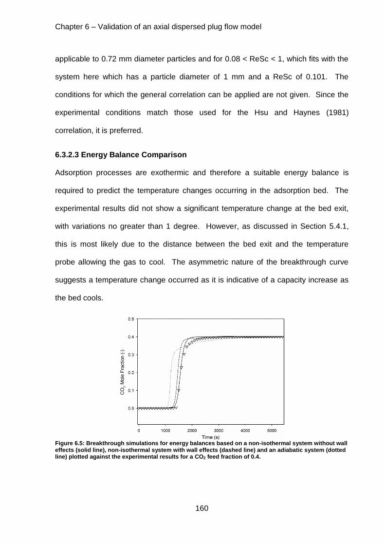
Chapter 6 – Validation of an axial dispersed plug flow model
160
applicable to 0.72 mm diameter particles and for 0.08 < ReSc < 1, which fits with the
system here which has a particle diameter of 1 mm and a ReSc of 0.101. The
conditions for which the general correlation can be applied are not given. Since the
experimental conditions match those used for the Hsu and Haynes (1981)
correlation, it is preferred.
6.3.2.3 Energy Balance Comparison
Adsorption processes are exothermic and therefore a suitable energy balance is
required to predict the temperature changes occurring in the adsorption bed. The
experimental results did not show a significant temperature change at the bed exit,
with variations no greater than 1 degree. However, as discussed in Section 5.4.1,
this is most likely due to the distance between the bed exit and the temperature
probe allowing the gas to cool. The asymmetric nature of the breakthrough curve
suggests a temperature change occurred as it is indicative of a capacity increase as
the bed cools.
Figure 6.5: Breakthrough simulations for energy balances based on a non-isothermal system without wall effects (solid line), non-isothermal system with wall effects (dashed line) and an adiabatic system (dotted line) plotted against the experimental results for a CO2 feed fraction of 0.4.
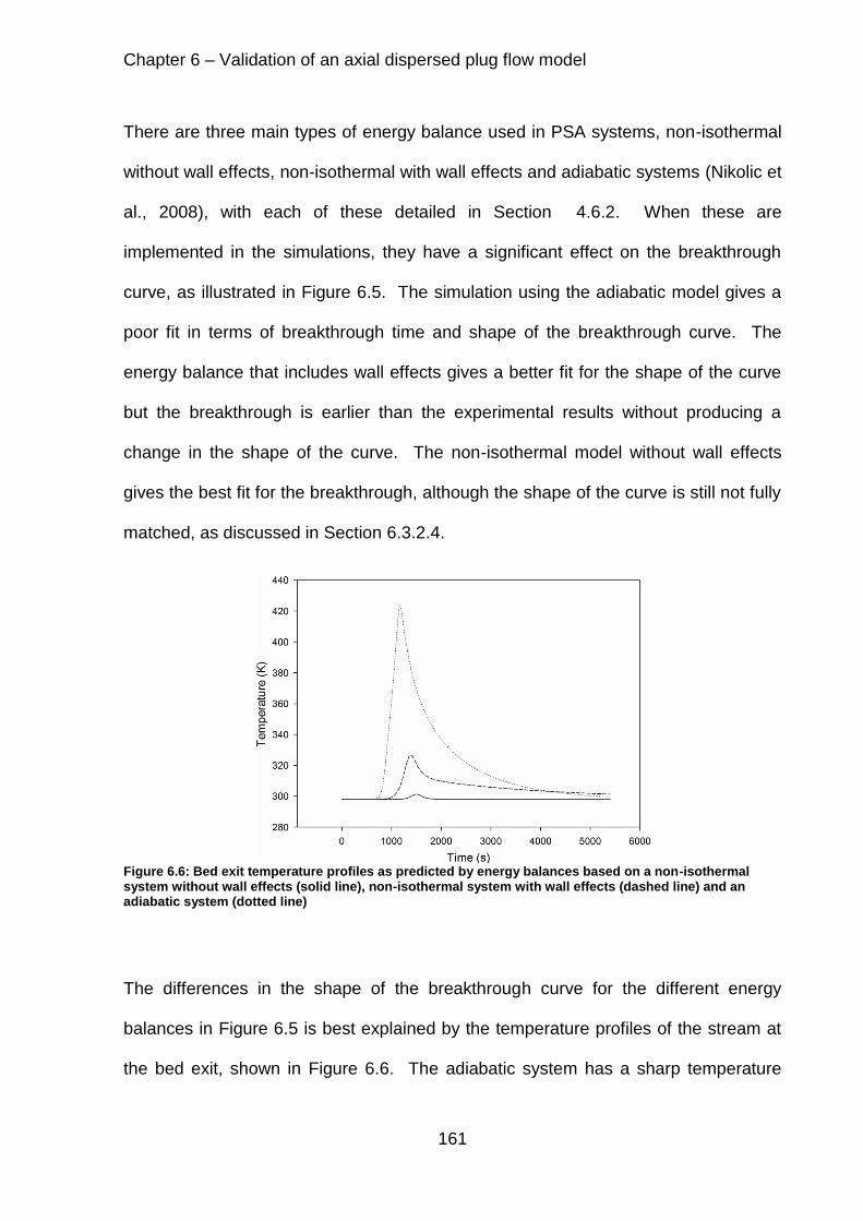
Chapter 6 – Validation of an axial dispersed plug flow model
161
There are three main types of energy balance used in PSA systems, non-isothermal
without wall effects, non-isothermal with wall effects and adiabatic systems (Nikolic et
al., 2008), with each of these detailed in Section 4.6.2. When these are
implemented in the simulations, they have a significant effect on the breakthrough
curve, as illustrated in Figure 6.5. The simulation using the adiabatic model gives a
poor fit in terms of breakthrough time and shape of the breakthrough curve. The
energy balance that includes wall effects gives a better fit for the shape of the curve
but the breakthrough is earlier than the experimental results without producing a
change in the shape of the curve. The non-isothermal model without wall effects
gives the best fit for the breakthrough, although the shape of the curve is still not fully
matched, as discussed in Section 6.3.2.4.
Figure 6.6: Bed exit temperature profiles as predicted by energy balances based on a non-isothermal system without wall effects (solid line), non-isothermal system with wall effects (dashed line) and an adiabatic system (dotted line)
The differences in the shape of the breakthrough curve for the different energy
balances in Figure 6.5 is best explained by the temperature profiles of the stream at
the bed exit, shown in Figure 6.6. The adiabatic system has a sharp temperature
Chapter 6 – Validation of an axial dispersed plug flow model
162
rise followed by a decaying curve that returns close to ambient temperature. The
magnitude of the steep temperature rise leads to a loss in the capacity which
explains the short breakthrough time. The decaying nature of the temperature profile
then gives rise to a breakthrough curve which tends to the inlet concentration
(Ruthven, 1984). The non-isothermal system with wall effects shows a smaller, but
not insignificant, peak and then a temperature decrease at a very low rate. This
leads to the breakthrough curve being steeper but then not quite reaching the final
concentration of carbon dioxide. The non-isothermal system without wall effects
leads to a slight temperature increase which cools rapidly so that the temperature
profile is symmetrical. This small temperature has the least effect on the
breakthrough time and the symmetrical temperature profile leads to a more
symmetrical breakthrough curve, meaning the asymmetric nature of the breakthrough
curve is not produced in the simulation.
Simulations that did not include wall effects have traditionally been used in literature
for PSA models (Farooq and Ruthven, 1990), where the temperature of the column
wall is assumed to be the same as the ambient temperature allowing the heat effects
to be lumped together. However, with increasing computational power, more recent
models, for both high pressure and low pressure systems, have included these
effects (Casas et al., 2012; Grande et al., 2013; Lopes et al., 2011). Without an
internal temperature profile or a temperature profile of the wall it is not possible to
validate the temperature profiles of the model. Therefore, the validation of the model
must rely on the breakthrough data which suggests that a model without wall effects
is the most accurate.

Chapter 6 – Validation of an axial dispersed plug flow model
163
6.3.2.4 Heat Transfer Coefficient Correlation Comparison
As discussed in Section 6.3.2.3, even with the inclusion of the energy balance the
asymmetrical shape of the breakthrough curve is not fully matched. The shape of the
simulation breakthrough curve is affected by the heat transfer rate from the gas
phase to the surroundings. The two main correlations considered for fixed beds are
the Leva (1947) correlation and the Yagi and Kunii (1960) correlation, detailed in
Section 4.7.3. Both correlations predict very similar values for the heat transfer
coefficient, with the Leva (1947) correlations and Yagi and Kunii (1960) predicting
values of 3.8x10⁻³ kJs-1m-2K-1 and 2.2x10⁻³ kJs-1m-2K-1 respectively. This leads to no
visible difference between two simulations with the same conditions. Several
literature models have used the Leva (1947) correlation to good success (Casas et
al., 2013a; Casas et al., 2012; Park et al., 1998) However, having reported the use of
the Leva (1947) correlation initially (Park et al., 1998), in subsequent work, Park et al.
(2000) suggested that the Leva (1947) correlation under predicts the heat transfer
rate at low mass fluxes, such as those used in that work and used here. For this
reason the Yagi and Kunii (1960).
The Yagi and Kunii (1960) correlation is based on the heat transfer coefficient when
the gas phase is stagnant,ℎ𝑤0 , and a fitting parameter, 𝛼𝑤. Yagi and Kunii (1960)
showed that the heat transfer coefficient becomes constant for systems with Re<30
and that the term with 𝛼𝑤 approaches zero. This means that the heat transfer
coefficient is the same as ℎ𝑤0 . Ofuchi and Kunii (1965) produced a graph which
predicts the heat transfer coefficient of the stagnant gas based on the ratio of solid to
fluid thermal conductivity but for the solid medium inside the bed rather than into the

Chapter 6 – Validation of an axial dispersed plug flow model
164
bed wall. The graph uses the dimensionless form of ℎ𝑤0 by multiplying it by the
characteristic length and dividing by the thermal conductivity of the fluid. This can be
applied to a fixed bed taking the characteristic length as the bed diameter instead of
the particle diameter. The ratio of thermal conductivities of stainless steel and the
gas mixtures is approximately 600. From this the graph presented by Ofuchi and
Kunii (1965) gives a value for the dimensionless group of 22. Based on the bed
diameter and fluid thermal conductivity, this predicts a value for ℎ𝑤0 of
22x10-2 kJs-1m-2K-1. This value is comparable to literature values. Park et al. (2000)
used a value of 4.2x10⁻² kJs-1m-2K-1 for a mixture of H2/CO2/CH4/CO using activated
carbon, found by using ℎ𝑤0 as a fitting parameter. Choi at al. (2004) give a final value
for the ℎ𝑤 as being 3.8x10⁻² kJs-1m-2K-1 in a methane and hydrogen separation over
activated carbon. The work by Ruthven et al. (1975) suggests a value of
19.7x10⁻² kJs-1m-2K-1 for propylene, cis-2-butene and 1-butene using zeolite 5A.
Figure 6.7: A comparison of simulations using values of 22x10-2
kJs-1
m-2
K-1
(solid line) and 4.2x10
2 kJs
-1m
-2K
-1 (dashed line) for the heat transfer coefficient of a stagnant gas with the experimental
data for a CO2 feed fraction of 0.4.

Chapter 6 – Validation of an axial dispersed plug flow model
165
A comparison of the value for ℎ𝑤0 predicted by the graph from Ofuchi and Kunii (1965)
and the value used by Park et al. (2000) is shown in Figure 6.7. The different values
do not have a significant effect on the breakthrough time or the shape of the
breakthrough curve simulated. Using a value of 4.2x10⁻² kJs-1m-2K-1 gives an SSD of
0.095 when combined for comparisons for all CO2 feed fraction and a value of
22x10-2 kJs-1m-2K-1 gives an SSD of 0.072. The lower value of ℎ𝑤0 appears to match
the shape of the breakthrough curve more accurately but breaks through sooner
giving the higher SSD. In this the system the accurate prediction of the breakthrough
time is required and so a value for ℎ𝑤0 of 22x10-2 kJs-1m-2K-1 is used.
6.4 Unmodified Activated Carbon PSA Cycle Modelling
Comparing simulations against the experimental data for breakthrough curves only
allows the adsorption step of a PSA cycle to be validated. The simplicity of the
experimental rig meant it was not possible to fully replicate a PSA cycle but it was
possible to produce experimental data for a 3 step and a 4 step process, as shown in
Section 5.6. Comparing the simulation output against the regenerative steps of a
PSA cycle shows the suitability of the model for developing a PSA cycle. Both the 3
step and 4 step experimental results are compared to corresponding simulations.
6.4.1 3 Step Cycle
A full description of a 3 step cycle is given in Section 3.7.3 and the model that can
replicate this is given in Section 4.11.3. The three step cycle includes an adsorption
step at elevated pressure, a depressurisation and purge step, where the feed is pure
nitrogen and in the first 60 seconds of the purge step the pressure is reduced to
atmospheric pressure, and a pressurisation step.

Chapter 6 – Validation of an axial dispersed plug flow model
166
Figure 6.8: 3 step breakthrough curves with their corresponding simulation at CO2 feed fractions of a) 0.1, b) 0.2, c) 0.3, d) 0.4 and e) 0.5
A comparison of the experimental carbon dioxide feed fraction at the bed exit for
each carbon dioxide feed fraction against the corresponding simulation for the
adsorption and purge step is given in Figure 6.8. The adsorption steps are the same

Chapter 6 – Validation of an axial dispersed plug flow model
167
as for the breakthrough curves reported in Figure 6.2. The two key points of
comparison for the purge step between the experimental and simulation data are the
shape of the curve and the peak value. For all of the simulations, the peak in carbon
dioxide in the outlet stream is accurately predicted during the depressurisation. This
shows that the controlled depressurisation model used, described in Section 4.11.3,
is able to replicate the depressurisation that is achieved by the back pressure
regulator in the experiment. The purge that continues after the depressurisation is
not simulated to the same degree of accuracy. The rate of decrease of carbon
dioxide is much faster in the simulation giving a shorter time for the bed to return to a
clean state. Table 6.4 shows the SSD for each carbon dioxide mole fraction and
separates this between the adsorption step and the entire regeneration step. The
regeneration step is more poorly matched than the adsorption step. The simulation
of PSA cycles is limited in literature. Cavenati et al. (2006) and subsequent work in
the same group by Lopes et al. (2011), did model a cyclic process. However, the
sampling technique was insufficient to show the detail of the desorption peak and so
these parts of the models are not validated. It is possible that the sudden changes in
pressure result in changes in the mass transfer resistances of the system which have
not previously been studied. However, a more likely cause is the empirical model for
a system without a fixed bed, discussed in Section 6.2, is not capable of predicting
the system response to the rapid change in pressure, flowrate and composition that
occurs. The empirical model for the surrounding system is validated for the
breakthrough of carbon dioxide at elevated pressure but has not been validated
against experiments with rapid changes in conditions. It is not possible to study the
rapid response of the surrounding system without the bed as the mass flow

Chapter 6 – Validation of an axial dispersed plug flow model
168
controllers are not able to replicate the sharp increase in flowrate as the bed
depressurises and desorption takes place. Schell et al. (2013) report a model used
for a complete PSA cycle, although their system did not return the bed to a fully
clean state. In their work, they are similarly not able to fully replicate the outlet
carbon dioxide fraction during the regeneration steps, with the model consistently
predicting a faster change in carbon dioxide fraction than is observed in their
experiments. They implement an empirical model based on a stagnant tank with an
improved fit to the experimental results.
Table 6.4: SSD between 3 step cycle experimental data and simulation data for the whole cycle and each of the steps for the unmodified activated carbon
0.1 0.2 0.3 0.4 0.5
Whole Cycle 0.060 0.062 0.072 0.075 0.083 Adsorption Step 0.017 0.018 0.018 0.014 0.015 Regeneration Step 0.080 0.078 0.088 0.092 0.102
The other aspect for comparison is the peak value predicted in the simulation
compared to the experimental result. The peak value of the 3 step desorption curve
indicates the selectivity of the material for carbon dioxide over nitrogen. The peak
values for the experimental data and the simulation data are presented in Table 6.5.
Carbon dioxide feed fractions of 0.2 and 0.3 are predicted to a good degree of
accuracy and the predictions at the other feed fractions are reasonable. For the
lowest carbon dioxide feed fraction, the simulation under predicts the peak value.
This is in agreement with Section 6.3.1, which suggests, based on the comparison of
the experimental and simulation breakthrough curves in Figure 6.2, the carbon
dioxide capacity is being under predicted for a feed fraction of 0.1. The simulations
of the two highest carbon dioxide feed fractions over predict the peak values which

Chapter 6 – Validation of an axial dispersed plug flow model
169
suggests at these feed fractions the selectivity is being over estimated. Considering
the good agreement for the breakthrough curve in Figure 6.2 which is dependent on
the carbon dioxide capacity, this would suggest the nitrogen capacity is being under
predicted. The closeness of the values suggests that the model is able to replicate
the changes occurring when the bed is depressurised. The same pattern between
the exit peak values as the carbon dioxide feed fraction increases is seen in Table
6.5 for both the experimental and simulation data, with the gap between the peak
values reducing each time.
Table 6.5: Comparison of the peak value of the desorption exit CO2 fraction at each CO2 feed fraction for the experimental and simulation data
CO2 Feed Fraction (-)
Experimental Peak Desorption Exit CO2 Fraction (-)
Simulation Peak Desorption Exit CO2 Fraction (-)
0.1 0.57 ± 0.009 0.53 0.2 0.69 ± 0.003 0.71 0.3 0.75 ± 0.009 0.77 0.4 0.77 ± 0.006 0.82 0.5 0.78 ± 0.006 0.85
Despite the discrepancies between the experimental and simulation data, the
agreement between the initial rise and the peak values suggests that the model is
able to replicate the majority of the effects that occur during the regeneration of the
bed in a PSA process.
6.4.2 4 Step Skarstrom Cycle
The 3 step cycle, although a useful indicator of the ability of the model to replicate
regeneration steps, is not representative of a typical PSA process in industry. The
most basic PSA cycle is a 4 step Skarstrom cycle which uses an adsorption step, a
blowdown step, a purge step and a pressurisation step, as fully described in Section
3.7.4. This separates the depressurisation and purge steps that are grouped

Chapter 6 – Validation of an axial dispersed plug flow model
170
together for a 3 step cycle. Therefore, during the blowdown step there is no flow
passing through the bed. This allows the carbon dioxide outlet fraction to reach a
maximum that is indicative of the selectivity of the material for the more adsorbed
product over the less adsorbed product. The other key difference to the 3 step cycle
is that the bed is not allowed to reach saturation, with the switch to the blowdown
step occurring when the carbon dioxide exit fraction reaches 5% of the inlet fraction.
As in the experiment, with the results presented in Section 5.6.2, the switch from the
adsorption step to the purge step occurs at 1510 s, which was determined from the
breakthrough curve.
Figure 6.9: CO2 exit mole fraction from experimental and simulation data for the adsorption, blowdown and purge steps of a 4 step Skarstrom cycle
The experimental and simulated CO2 exit mole fractions for the first three steps of a 4
step Skarstrom cycle are reported in Figure 6.9. There is good agreement between
the two, especially in the blowdown step. The overall cycle has an SSD of 0.050,
with the blowdown and purge step having SSD values of 0.051 and 0.062
respectively. There is a slight discrepancy in the time for the system to reach the

Chapter 6 – Validation of an axial dispersed plug flow model
171
maximum value, with the simulation reaching 99% of the maximum value 120
seconds sooner than the experimental data reaches 99% of its maximum value. The
maximum values differ slightly, with the average experiment maximum at an exit
fraction of 0.983 ± 0.06 and the simulation maximum at an exit value of 0.996. The
maximum values for the 3 step cycle in Table 6.9 indicate that the simulation is over
predicting the selectivity for carbon dioxide over nitrogen. This is further confirmed
here with the simulation giving a higher maximum value than the experimental
results.
As with the 3 step cycle, the carbon dioxide outlet fraction data presented in Figure
6.9 shows that the simulation predicts the bed being fully clean at an earlier time than
is observed in the experimental data. The initial part of the purge step is replicated
accurately but as the outlet carbon dioxide fraction approaches approximately 0.3,
the simulation does not predict the same reduction in the rate the carbon dioxide
outlet fraction is decreasing. The explanation for this is most likely to be
measurement delays that occur in the experimental rig as suggested by Schell et al.
(2013). However, this does not have the same rapid change in pressure as the three
step cycle and so could indicate the simulation is not able to predict a mass transfer
limitation for the purge step. It is not possible to be certain as very little work has
investigated the validation of the regeneration steps for PSA systems.
Overall, the agreement between the experimental and simulation data gives
confidence to further develop the model in order to represent effects of different PSA
cycles. Being able to replicate the breakthrough time is key as this dictates the
length of a step in the cycle. The first half of the purge step is also very important as
a full cyclic PSA process would not return the bed to a clean state, as shown by

Chapter 6 – Validation of an axial dispersed plug flow model
172
Schell et al. (2013). Therefore, the model accurately represents the aspects of the
experimental data which are most important for a PSA system.
6.5 Modified Activated Carbon Modelling
In order to test the flexibility of the model, simulations were produced for the
separation of CO2/N2 mixtures using the modified activated carbon. For this, the
assumptions and correlations used for the unmodified material were used, i.e.
multicomponent DSL, the Hsu and Haynes (1981) correlation for the dispersion
coefficient, an energy balance without wall effects, the Yagi and Kunii (1960)
correlation for the heat transfer coefficient and a stagnant heat transfer coefficient of
22x10-2 kJs-1m-2K-1. The parameters that have been changed from Table 6.1 are
given in Table 6.6. The extended DSL temperature independent parameters for the
modified activated carbon are reported in Table 5.8.
Table 6.6: Parameters for the simulation of CO2/N2 breakthrough separations using modified activated carbon
Bed Length m 0.065 Bed Density kg m3 191 Particle Diameter m 1 x 10⁻³
Pore Diameter m 1.76 x 10⁻⁹
Bed Voidage - 0.4 Particle Voidage - 0.85 CO2 Heat of Adsorption kJ mol-1 26.6 N2 Heat of Adsorption kJ mol-1 15.7
6.5.1 Breakthrough Modelling
A comparison between the experimental breakthrough data at each of the carbon
dioxide feed fractions tested and their corresponding simulation is presented in
Figure 6.10. The SSD and percentage difference in breakthrough time are reported
in Table 6.7. Excellent agreement is seen between the simulation and experiment for

Chapter 6 – Validation of an axial dispersed plug flow model
173
a carbon dioxide feed fraction of 0.2. There is a slight over prediction of the
breakthrough time for a carbon dioxide feed fraction of 0.1 but the shape of the
breakthrough curve is well matched, as evidenced by the low SSD. The
breakthrough curves for carbon dioxide feed fractions of 0.3, 0.4 and 0.5 are all
under predicted by the model, the extent of which increases at higher feed fractions.
The cause of this stems from the isotherm model used. The carbon dioxide capacity
predicted by the multicomponent DSL model, discussed in Section 5.5.1.1 and
reported in Table 5.18, shows that the DSL model does not predict the change in
capacity between 0.2 and 0.5 to be as large as the experimental results. The
increase in capacity for a breakthrough with a carbon dioxide feed fraction of 0.4 to
0.5 is predicted to be 0.35 mol kg-1 for the DSL isotherm model but 0.64 mol kg-1 for
the experimental data. This suggests that for the modified material, the isotherm
model is not able to predict the breakthrough capacities at higher feed fractions.
Figure 6.10: Simulation break through curves for the modified activated carbon material plotted against the corresponding experimental data with CO2 feed fraction of 0.1 (white circles), 0.2 (white squares), 0.3 (black triangles), 0.4 (white triangles) and 0.5 (black diamonds).

Chapter 6 – Validation of an axial dispersed plug flow model
174
Grande et al. (2013) reported similar under predictions of the breakthrough capacity
at elevated pressures, however, this did not lead to under predictions of the
breakthrough curve with their simulation results giving significantly longer
breakthrough times than their experimental data for the highest pressures used. The
results for the modified material differ from those for the unmodified material shown in
Figure 6.2, where the lower feed fractions were not as well represented as the higher
feed fractions. The results presented by Grande et al. (2013) and the results
reported here show that the carbon dioxide capacity at elevated pressures is difficult
to predict accurately.
Table 6.7: SSD values and the difference in breakthrough time for the comparison of the best fit simulation to the experimental breakthrough data for modified activated carbon.
CO2 Feed Fraction
SSD Breakthrough
Time Difference
0.1 0.0083 -19.6% 0.2 0.0059 -1.8% 0.3 0.0275 5.5% 0.4 0.0460 7.6% 0.5 0.0655 9.1%
Total 0.1531 -
The shape of the simulation breakthrough curves in Figure 6.10 is similar to the
experimental curves for carbon dioxide feed fractions of 0.1 and 0.2. However, for
the higher carbon dioxide feed fractions, the simulations do not show the same
degree of spreading as the experimental data. This is similar to the higher carbon
dioxide feed fractions for the unmodified material in Figure 6.2, where the
asymmetrical nature of the breakthrough curve was not represented. In both cases it
is likely that the temperature change is not being fully accounted for, as a higher
temperature rise and subsequent cooling would cause the breakthrough curve to

Chapter 6 – Validation of an axial dispersed plug flow model
175
spread at the top. This is less important for the lower carbon dioxide feed fractions
as the temperature rise is smaller and therefore the effect is less prominent. This
suggests that the dispersion and mass transfer taking place is being accurately
predicted by the correlations used. It is possible to use different correlations for the
heat transfer coefficient to predict greater temperature changes. However, as
discussed in Section 6.3.2.4, increased temperature changes result in the
breakthrough time not being accurately represented, which is the focus of this work.
As with the unmodified material, a significant temperature rise was not observed in
the experimental temperature profile for the modified material and so it is also not
possible to validate the temperature change taking place.
6.5.2 PSA Cycle Modelling
As with the unmodified material, simulations were carried out to replicate the PSA
cycles for the modified activated carbon. A description of the simulation of 3 and 4
step cycles is given in Section 3.7.
6.5.2.1 Three Step Cycle
A comparison of the experimental data for a 3 step cycle and the simulation data for
each CO2 feed fraction for the adsorption and purge step in a 3 step cycle is
presented in Figure 6.11. The adsorption step matches the results of the
breakthrough curves reported in Figure 6.10. For the purge step, the initial increase
in exit carbon dioxide mole fraction is accurately simulated but the peak value and
the decrease in exit carbon dioxide mole fraction are not well matched. Table 6.8
reports the normalised SSD for each of the carbon dioxide mole fractions. The
standard difference between the experimental and simulation data for the
regeneration step is much larger than the adsorption step. The regeneration step

Chapter 6 – Validation of an axial dispersed plug flow model
176
values are comparable to the SSD values for the unmodified activated carbon
reported in Table 6.4. The initial increase shows that the general behaviour is being
replicated. The discrepancy in the peak values between the simulation and
experimental data is quantified in Table 6.9. The model is predicting a much higher
selectivity for the carbon dioxide over nitrogen than is being observed in the
experiment. The most likely explanation is that the isotherm is not accurately
predicting the capacity for nitrogen. Garcia et al. (2013) showed that for CO2/H2
mixtures the DSL model tended to under predict the hydrogen uptake, especially at
low CO2 feed fractions. The extended DSL isotherm predicts low nitrogen capacities,
given in Table 5.18, due to the interaction of the parameters on the two sites for the
DSL isotherm, suggesting a high selectivity for carbon dioxide over nitrogen. In
contrast to the poor agreement for the modified material, the peaks for the purge step
using the unmodified activated carbon match with reasonable accuracy, as shown in
Table 6.5. The predicted selectivities using the multicomponent DSL isotherm for the
unmodified and modified activated carbons are given in Table 6.10. The predicted
carbon dioxide selectivities for the unmodified material are considerably lower than
the modified material and explain the much higher peak values predicted for the
modified material in Table 6.9.
Table 6.8: SSD between 3 step cycle experimental data and simulation data for the whole cycle and each of the steps
0.1 0.2 0.3 0.4 0.5
Whole Cycle 0.065 0.064 0.075 0.082 0.093 Adsorption Step 0.009 0.006 0.032 0.050 0.076 Regeneration Step 0.089 0.084 0.091 0.096 0.102

Chapter 6 – Validation of an axial dispersed plug flow model
177
Figure 6.11: 3 step breakthrough curves for modified activated carbon with their corresponding simulation at CO2 feed fractions of a) 0.1, b) 0.2, c) 0.3, d) 0.4 and e) 0.5
Table 6.9: Comparison of the peak value of the desorption exit CO2 fraction at each CO2 feed fraction for the experimental and simulation data for the modified activated carbon
CO2 Feed Fraction (-)
Experimental Peak Desorption Exit CO2
Fraction (-)
Simulation Peak Desorption Exit CO2 Fraction (-)
0.1 0.51 ± 0.015 0.71 0.2 0.63 ± 0.006 0.80 0.3 0.70 ± 0.003 0.84 0.4 0.71 ± 0.029 0.87 0.5 0.74 ± 0.008 0.90

Chapter 6 – Validation of an axial dispersed plug flow model
178
In a similar way to the unmodified material in Figure 6.8, Figure 6.11 shows the
simulation is unable to match the purge of the bed after depressurisation for the
modified material. The simulation predicts a more rapid decrease in the exit carbon
dioxide mole fraction than is observed in the experiment. This is most likely due to
the empirical model for the surrounding system being unable to predict the system
response to the rapid changes in pressure and mole fraction. This is similar to the
issues that Schell et al. (2013) reported in predicting the purge step.
Table 6.10: Comparison of the selectivity for carbon dioxide over nitrogen based on the multicomponent DSL isotherm calculated by dividing the carbon dioxide capacity by the nitrogen capacity.
Predicted Carbon Dioxide Selectivity over Nitrogen for the Unmodified Activated Carbon
Predicted Carbon Dioxide Selectivity over Nitrogen for the
Modified Activated Carbon
1.5 9.0 3.3 22.3 5.7 40.3 8.7 61.4
12.9 96.5
6.5.2.2 4 Step Skarstrom Cycle
A comparison for a 4 step Skarstrom cycle was conducted between the experimental
results and simulations. The four steps simulated were a pressurisation step (not
shown), an adsorption step, a 600 second blowdown step with depressurisation
occurring in the first 60 seconds and a 2100 second purge step. As with the
experimental results, the system is switched from the adsorption step to the
blowdown step after 1260 seconds. The experimental results for a 4 step Skarstrom
cycle are compared to simulation results in Figure 6.12. Strong agreement is seen
for the initial breakthrough in the adsorption step. This gives credence to the
importance of the model predicting the breakthrough time over the shape of the

Chapter 6 – Validation of an axial dispersed plug flow model
179
breakthrough curve that was discussed in Section 6.3.2. The SSD for the whole
cycle is 0.049, which is skewed by the adsorption step as these points match
perfectly. The blowdown step has a SSD of 0.077 and the purge step has a value of
0.053.
Figure 6.12: CO2 exit mole fraction from experimental and simulation data for the adsorption, blowdown and purge steps of a 4 step Skarstrom cycle using modified activated carbon
The blowdown step occurs from 1260s to 1860s. The initial rise is well replicated but
the broadening of the experimental curve as the system reaches equilibrium is not
represented by the simulated results. As with the unmodified material, this is most
likely due to the response of the surrounding system taking time to equilibrate.
During the 60 second depressurisation the velocities through the CO2 analyser are
very high but after this there is no flow through the system so the equilibration needs
to occur by diffusion. There might also be some lag in the system due to the 75
second response time of the analyser. The average maximum value for the
experimental data was 0.985 ± 0.011 whereas the maximum value for the simulation
was 0.9996. The maximum value for the simulation suggests a selectivity for carbon

Chapter 6 – Validation of an axial dispersed plug flow model
180
dioxide over nitrogen of 2500, which is unlikely considering the capacity shown for
the pure component isotherms. This is the same discrepancy that was observed for
the 3 step model and emphasised by the high selectivities that the DSL isotherm
predicts in Table 6.10. This further suggests that the nitrogen capacity is being under
predicted by the multicomponent DSL isotherm.
The purge curve shown in Figure 6.12 is represented to a high degree of accuracy.
Towards the lower exit carbon dioxide mole fractions, the simulation predicts a
slightly higher rate of decrease than the experimental data. The SSD for the purge
step of 0.053 is lower than any other cyclic simulation. It indicates a better fit than
for the purge step of the unmodified material which has an SSD of 0.062. Compared
to the 3 step, which had an SSD of 0.088 for the unmodified material and 0.092 for
the modified material, the fit is considerably better. This indicates that the 3 step
cycle model is not predicting the purge step as the system cannot respond to the
sudden change in pressure and flowrate. However, for the four step cycle model it is
possible to replicate the purge curve to a higher degree of accuracy.
6.6 Parameter Sensitivity Analysis
The main use for the model is to test adsorbents for their suitability for use in PSA
systems. However, it can also be used to aid design of adsorbent materials by
investigating which properties of the material have the biggest effect on the
breakthrough curves, both in terms of the breakthrough time and the shape of the
breakthrough curve. It is clear that for a given system it is desirable to have a long
breakthrough time and a steep breakthrough curve as this maximises the use of the
bed. Several parameters that can be controlled by the design of the adsorbent
pellets were varied within the model and the breakthrough curves compared. For

Chapter 6 – Validation of an axial dispersed plug flow model
181
each parameter a base case was established based on the parameters for the
unmodified activated carbon as given in Table 6.1. The parameter was then varied,
whilst keeping all other parameters constant, and the breakthrough curves
compared. There were three parameters that had a significant effect on the
breakthrough curve, the particle diameter, the bed voidage and the particle voidage.
These results are reported in the subsequent sections.
6.6.1 Particle Diameter
Figure 6.13: Sensitivity analysis for particle diameters of 1 x 10⁻⁴
m (dotted line), 5 x 10⁻⁴
m (short dashed line), 1 x 10
-3 m (solid line), 2.5 x 10
-3 m (long dashed line) and 5 x 10
-3 m (dashed and dotted line).
The particle diameter affects the gas flow through the system and the pressure drop
across a bed, resulting in a noticeable effect on the breakthrough curve. It was
assumed that a change in particle diameter did not affect any other properties in the
bed, i.e. the bed voidage remained constant. The correlations used for parameters
such as the dispersion coefficient are built into the model and therefore varied
appropriately. It was assumed that all correlations were valid for all particle
diameters tested. The breakthrough curves for particle diameters of 0.1, 0.5, 1, 2.5

Chapter 6 – Validation of an axial dispersed plug flow model
182
and 5 mm beads are given in Figure 6.13. As the particle diameter increases, the
shape of the breakthrough curve is severely affected. The breakthrough capacity
remains almost constant, as evidenced by the same fixed point at which all of the
curves cross at. The capacity is expected to remain constant, as observed, since the
particle diameter does not affect the adsorption capacity of the material or the
amount of material in the system.
Table 6.11: Predicted values for the Reynolds number, dispersion coefficient, overall CO2 mass transfer coefficient, CO2 film mass transfer effect and CO2 pore mass transfer effect at the particle diameters simulated
Particle Diameter
(m)
Reynolds Number
(-)
Dispersion Coefficient
(m2 s-1)
Overall CO2 Mass
Transfer Coefficient
(s-1)
CO2 Film Mass
Transfer (s-1)
CO2 Pore Mass
Transfer (s-1)
1 x 10⁻⁴ 0.12 2.31 x 10⁻⁷ 0.158 49.2 42.7 5 x 10⁻⁴ 0.49 6.75 x 10⁻⁷ 0.137 2.36 1.71 1 x 10⁻³ 1.22 1.50 x 10⁻⁶ 0.099 0.67 0.43
2.5 x 10⁻³ 3.05 4.37 x 10⁻⁶ 0.035 0.14 0.068 5 x 10⁻³ 6.10 9.41 x 10⁻⁶ 0.011 0.043 0.017
As discussed in Section 5.4.1, the shape of the breakthrough curve is strongly
dependent on the dispersion taking place and the mass transfer limitations. For each
of the particle diameters tested, the values of the dispersion coefficient and the mass
transfer coefficient that are predicted by their corresponding correlations are reported
in Table 6.11. The dispersion coefficient is the degree of turbulent spreading that is
occurring and therefore is greater at higher Reynolds numbers. An increase in
particle diameter increases the turbulence in the system and therefore leads to a
significant increase in the dispersion taking place. The mass transfer limitations also
greatly increase as the particle diameter increases. The overall carbon dioxide mass
transfer coefficient and the contribution of film and pore mass transfer limitations are

Chapter 6 – Validation of an axial dispersed plug flow model
183
reported in Table 6.11. The third mass transfer effect, the micropore mass transfer,
is assumed to have a constant contribution of 0.158 s-1 as this would be unaffected
by the size of the particle used (Ruthven, 1984). It is clear that an increase in particle
diameter significantly increases the mass transfer limitations. At very low particle
diameters, only the micropore resistance is significant but above particle diameters of
1 mm, the film and pore mass transfer resistances become the controlling influences.
As discussed by Garg and Ruthven (1975), the mass transfer and dispersion effects
are additive. Therefore, the greater dispersion and higher mass transfer effects lead
to an increase in the degree of spreading that is occurring in the system. The effects
are not as significant as the particle diameter decreases below 1 mm. Below this
value the dispersion effects become negligible and the mass transfer is only limited
by micropore diffusion. However, above 1 mm, small increases in particle diameter
are seen to have very large effects. It can be inferred from this, therefore, that
particle diameters should be minimised. Small particle sizes, however, have a
detrimental effect on the pressure drop across the bed. The effects are not seen
here as the bed is too small, but at industrial scale the pressure drop would increase
rapidly as the particle size diminished (Mehta and Hawley, 1969). Therefore, a
compromise would be needed between the two effects which could be quickly judged
by use of the model presented here.
6.6.2 Bed and Particle Voidage
The voidage in the system indicates the amount of active adsorbent material in the
bed. As discussed in Section 5.5.1.2, the carbon dioxide capacity on a volumetric
basis rather than a mass basis is a much better indicator of the capacity of a PSA
system for a fixed volume bed. Therefore, it is important to consider the bed density

Chapter 6 – Validation of an axial dispersed plug flow model
184
that a given adsorbent would have. The degree to which modifying the bed density
of the system affects the breakthrough curves has been tested by modifying the bed
and particle voidages.
Figure 6.14: Sensitivity analysis for bed voidages of 0.3 (dotted line), 0.4 (short dashed line), 0.48 (solid line), 0.6 (dashed and dotted line) and 0.7 (long dashed line)
The bed voidage cannot be modified without affecting the bed density. Therefore,
the bed density is modified accordingly to match a chosen bed voidage. This was
achieved by assuming the material and particle densities remain constant, i.e. the
particle was manipulated in such a way that the packing of the material changed
without the material itself being modified. Simulations using voidages of 0.3, 0.4,
0.48, 0.6 and 0.7 were investigated as voidages can range from the densest regular
packing for rhombohedral with a bed porosity of 0.26 up to the loosest forms with bed
porosities of 0.88 (Dullen, 1979). Breakthrough curves for these simulations are
plotted in Figure 6.14. It is apparent that the main effect is on the breakthrough time
rather than the shape of the breakthrough curve. There is slightly more spreading
observed for lower values of bed voidage as the interstitial velocity will be higher for a

Chapter 6 – Validation of an axial dispersed plug flow model
185
smaller bed voidage. However, this effect is minimal compared to the change in
capacity.
With a particle density of 500 kg m-3, an increase in bed voidage of 0.1 results in a
bed density decrease of 50 kg m-3. Therefore a bed voidage of 0.3 has a bed density
of 350 kg m-3 and a bed voidage of 0.7 has a bed density of 150 kg m-3. This means
at lower bed voidages there is more active adsorbent present, increasing the
capacity of the overall system. Therefore, the design of any adsorbent should alter
the shape of the material to increase the packing as this increases the carbon dioxide
capacity.
Figure 6.15: Sensitivity analysis for particle voidages of 0.6 (dotted line), 0.7 (short dashed line), 0.75 (solid line), 0.8 (dashed and dotted line) and 0.9 (long dashed line)
The particle voidage also has a significant role to play in the capacity of a given
system. In order to vary this, it is assumed that the material density and the bed
voidage remain constant. The particle and bed density can then be calculated for a
chosen particle voidage. The simulation was run using particle voidages of 0.6, 0.7,

Chapter 6 – Validation of an axial dispersed plug flow model
186
0.75, 0.8 and 0.9 and corresponding bed densities of 534, 428, 321, 262, 214 and
107 kg m-3. This covers the full range of particle voidages possible for activated
carbons (Dullen, 1979). The results of the simulations are presented in Figure 6.15.
The shape of the breakthrough curve is unaffected as the flow regime is not impacted
by the particle voidage and has a minimal effect on the mass transfer effects. The
breakthrough capacity is strongly affected as there is more of the adsorbent in the
same bed volume. In a similar way to the bed voidage, decreasing the particle
voidage has a strong effect on the overall capacity and should be minimised to
increase the capacity.
The degree to which changes to the bed and particle voidages affect the capacity of
the system highlight the importance of maximising the amount of activated material.
This is only an indication and might not possibly take in to account all of the effects
that a change in bed voidage and particle voidage might have. Modifications to
activated carbon tend to be based on opening up more of the pore structure which
increases the pore volume (Chen et al., 2013). However, this increase in pore
volume is more detrimental due to the decrease in bed density without giving
sufficient increases in the adsorption capability of the material itself. This model
shows that the focus needs to be on the structure of the material and maximising the
bed density without reducing the capacity of the material.
6.7 Conclusion
A model has been established and validated against experimental data. This was
first performed using the breakthrough curves for the separation of CO2/N2 mixtures
using the unmodified activated carbon. By careful selection of suitable correlations,
the model was able to simulate the breakthrough curves to a reasonable degree of

Chapter 6 – Validation of an axial dispersed plug flow model
187
accuracy using independent values for the parameters rather than fitting the model to
the experimental data. The model was then further validated against cyclic
experimental data for the unmodified material. The 3 step and 4 step model was
simulated to a good degree of accuracy, although the purge step in the simulation
was faster than the experimental data.
The breakthrough curves for the modified material are not as accurately simulated.
The breakthrough results suggest that the system requires an isotherm that predicts
a higher capacity for carbon dioxide at higher carbon dioxide partial pressures. The
PSA cycle simulations also suggest that the predicted nitrogen capacity needs to be
higher as the selectivities found in the experiments are significantly lower than those
predicted by the simulation. The purge step for the 4 step cycle is accurately
represented, giving an overall good prediction of the 4 step cycle, with important
variables such as the breakthrough time accurately predicted. This gives evidence
for choosing parameters that can accurately predict the breakthrough time. The
reasonable agreement suggests, to a first approximation, this model would be
capable of indicating the most suitable way to operate a PSA system.
A parameter sensitivity study has shown that there are relatively few material
parameters which strongly affect the breakthrough of a system. The particle
diameter, bed void and particle void have a significant effect on the breakthrough
curve. The particle diameter affects the shape of the breakthrough curve as the
dispersion and mass transfer are sensitive to changes in it. Above 1 mm diameter
particles, the spreading becomes significant. This suggests that in the design of a
particle, the critical diameter, above which dispersion and mass transfer effects
occur, needs to be found. Both the bed void and particle void affect the volume of

Chapter 6 – Validation of an axial dispersed plug flow model
188
active material in a given fixed bed. In both cases lower voids result in longer
breakthrough times without significant effects on the shape of the breakthrough
curve. The extremes that were tested may not be achievable but it adds further
evidence to the findings in Chapter 5 that the bed density needs to be maximised
either through the design of the particle and packing of the bed or through the design
of the material itself.
The model has been established in such a way that by knowing the dimensions of
the bed, the physical characteristics of the adsorbent and the temperature dependent
isotherm parameters, the system can be modelled straightforwardly. This can then
be used to compare the dynamic response of the system to a first approximation
without requiring experiments to be conducted which require a reasonable amount of
the material to be produced. The validation of the model means it can be used to
investigate the properties of a PSA system, which is done in Chapter 7.

Chapter 7– Pressure Swing Adsorption Cycle Development
189
Chapter 7 – Pressure Swing Adsorption Cycle Development
Chapter 7– Pressure Swing Adsorption Cycle Development
190
7.1 Introduction
The model presented and validated in Chapter 6 has been applied to develop
pressure swing adsorption (PSA) systems that capture of carbon dioxide from syngas
in integrated gasification combined cycle (IGCC) power plants. This is based on the
possibility of them being less expensive and more efficient than the liquid absorption
counterparts (Radosz et al., 2008). The removal of carbon dioxide from syngas by a
PSA system presents a relatively unique situation in requiring the maximum purity
and capture rate of both the heavy and light components. For post-combustion
carbon dioxide capture only the carbon dioxide product is important as the nitrogen
product is simply vented. Other more traditional systems also only captured one
product, often the light product. The development of PSA processes was realised in
the Skarstrom cycle aimed at producing oxygen and the process has been widely
applied to hydrogen production, where the more strongly adsorbed components are
not required (Ruthven, 1984).
The application of PSA systems for the recovery of both the light and heavy
component at high pressures has not been widely studied. Casas et al. (2013b)
have produced the most comprehensive study, studying a 10 step process and the
conditions that affect the purity of the gases produced and the amount of each gas
that is captured in the product. Schell et al. (2013) validated a 6 step model against
experimental results without optimising the system. The work mainly aimed to
validate the experimental set-up and therefore little consideration was given to
producing the best process design. Agarwal et al. (2010) developed a
superstructure-based simulation that was able to design a process for the separation
of CO2/H2 mixtures for pre-combustion capture based on maximising the carbon

Chapter 7– Pressure Swing Adsorption Cycle Development
191
dioxide capture rate and purity whilst minimising the power consumption of the
system. Xiao et al. (2009) investigated a vacuum pressure swing adsorption (VPSA)
system for the separation of carbon dioxide from syngas at elevated temperatures
and pressures.
The main aim of these studies was to produce a high quality carbon dioxide product,
with Agarwal et al. (2010) being the only one to detail the quality of the light product
but without carrying out an optimisation of any aspect of this. The main effect that a
PSA system would have on the efficiency of an IGCC power plant is the loss of
hydrogen. Therefore, it is very important to minimise this loss and it must be taken
into consideration when evaluating PSA systems. The literature work also does not
highlight the impact that each process step has on the overall system performance.
The systems described have been studied to prove if the concept is capable of
producing sufficient quality carbon dioxide product. However, in order to advance
this technology the importance of each step in a PSA cycle needs to be understood
to be able to evaluate which aspects are economically viable.
The work presented in this chapter addresses these issues to give a fuller
understanding of the PSA processes which could be applied for industrial carbon
capture processes. The simulations have been carried out to study the separations
of CO2/N2 mixtures, as this was the separation validated in Chapter 6. Therefore, the
quantitative values found for the quality of the gases produced will not be directly
applicable to IGCC operations. However, the impact that each process step has on
the quality of gases will be translatable to that process. The work is presented in
such a way so as to build the PSA process from a basic 4 step Skarstrom cycle to a
10 step cycle implementing pressure equalisation, purge gas recovery and the use of

Chapter 7– Pressure Swing Adsorption Cycle Development
192
a heavy product rinse. Each of the new steps are evaluated to understand the effect
they have on the quality of both the carbon dioxide product and the nitrogen product.
7.2 Model Set-Up
The aim of this chapter is to investigate different process configurations and to
suggest improvements for the development of a PSA process for the capture of
carbon dioxide from IGCC power plants. In order to do this a consistent model needs
to be used. The axial dispersed plug flow model that is described in Section 4.6 is
implemented. The only difference to the validated model is that the multicomponent
Langmuir-Freundlich (LF) isotherm is used instead of the Dual-site Langmuir (DSL)
isotherm. It was found that the LF isotherm gave a higher model stability which
became important for PSA processes with a large number of beds and many
discontinuities. The effect of using these two isotherms on the system is described in
Section 6.3.2.1, where the DSL isotherm is shown to give a better fit to the
experimental data. The LF model under predicts the breakthrough time by 6.9%
compared the DSL model under prediction of 4.2%. However, as this chapter aims
to study the aspects of a PSA cycle which will give significant process gains, the
small under prediction for breakthrough time given by the LF isotherm will not affect
the recommendations made.
Table 7.1: Gas stream feed conditions
Flowrate (mol s-1) 7.2 x 10⁻⁵
Pressure (Pa) 2.5 x 10⁶ Temperature (K) 298 CO2 Mole Fraction
(-) 0.4
N2 Mole Fraction (-) 0.6

Chapter 7– Pressure Swing Adsorption Cycle Development
193
All other parameters are unaffected and remain the same as for the model used in
Section 6.3.1. The feed stream is kept the same for all process configurations tested
and these properties are given in Table 7.1. A full description of the solver set-up,
the model configuration and the solution methods are given in Chapter 4.
7.3 Four Step Cycle
The Skarstrom cycle is the simplest PSA cycle, developed initially for separating
oxygen and nitrogen. It has four basic steps: adsorption, blowdown, purge and
pressurisation. The conditions of each of these steps can vary as well as the
duration of each step so that it can be applied to a wide range of industrial
separations (Ruthven, 1984). A 4 step Skarstrom cycle was validated against
experimental data in Section 6.4.2. Here the conditions are altered for the cycle in
order to maximise the carbon dioxide and nitrogen purities and capture rates.
Figure 7.1: 4 bed 4 step Skarstrom process configuration showing a) bed connections and b) bed sequencing. Ad – adsorption, BD – blowdown, Pur – purge with feed, Press – pressurisation.
A typical 4 step cycle is shown in Figure 7.1. The four process steps use high
pressure adsorption, blowdown, purge step by a fraction of the feed gas and a
a) b)

Chapter 7– Pressure Swing Adsorption Cycle Development
194
pressurisation step using a fraction of the feed gas. In order to realistically represent
a PSA process unit some modifications were made to the model used in Section
6.4.2. These are mainly concerned with the adjustment of the feed conditions. First
of all it was assumed that the pressurisation gas has the same properties of the
adsorption feed gas stream rather than a pure nitrogen stream. In the industrial
process the feed gas stream is at an elevated pressure and can therefore be used to
pressurise the bed without the need for any additional equipment such as a
compressor. The other key change is to purge the bed with a fraction of the feed gas
stream. The main reason to use a pure nitrogen purge is to return the bed to a clean
state, i.e. minimise the residual carbon dioxide in the bed. This results in a high
nitrogen purity but reduces the nitrogen capture rate. For a gas turbine the purity of
the light product would not need to be particularly high as a gas turbine can operate
across a range of hydrogen concentrations (Miller, 2011). The use of a fraction of the
feed gas for purging the system has been employed previously when the heavy
product is also required (Casas et al., 2013b; Schell et al., 2013). This also limits the
dilution of the heavy product by the light product.
It is possible to operate the bed in both a co-current and counter-current operation.
In counter-current operation the gas flows in the opposing direction to the adsorption
step during blowdown and purge step. This is used to minimise the amount of the
more strongly adsorbed product in the light product (Ruthven, 1984). However, due
to the desire to capture both the light and heavy product, the effect of using counter-
current steps was evaluated. As there are no interactions between the 4 beds during
the cycle, only one bed is simulated to reduce the computational time. The other
beds are assumed to operate in the same way but one quarter of a cycle out of sync

Chapter 7– Pressure Swing Adsorption Cycle Development
195
with the previous cycle as shown in Figure 7.1. This was tested by running a
simulation using 4 beds and there was no difference between the results for each
bed. For the one bed operation the time was kept constant for each step by
recording the adsorption time and then using this as the step length for the remaining
steps in each cycle.
The co-current and counter-current operations were compared by running the two
scenarios under the same conditions, given in Table 7.2. The feed stream is split
between the adsorption, purge and pressurisation steps. The fractions were found
iteratively in such a way that the length of the adsorption and pressurisation step
would be the same. The fraction for the purge step was chosen to give the required
cleaning of the bed whilst minimising loss of nitrogen. The purity of the carbon
dioxide outlet set as the breakthrough point is chosen as a balance between the
carbon dioxide and the nitrogen purity. The results reported are for the third cycle of
a system and at this point the system has reached cyclic steady state, judged by the
adsorption time for all beds matching the adsorption time of the previous step.
Table 7.2: Feed conditions and set adsorption switch point for a 4 step Skarstrom cycle
Feed Fraction for Adsorption (-) 0.45 Feed Fraction for Purge (-) 0.1 Feed Fraction for Pressurisation (-) 0.45 CO2 Mole Fraction Breakthrough Point (-) 0.22
7.3.1 Cyclic Outputs
The pressure profile for both operations is reported in Figure 7.2 as the counter-
current operation does not affect the pressure profile at the bed exit. The blowdown
step shows the reduction in pressure. This is non-linear and is controlled by

Chapter 7– Pressure Swing Adsorption Cycle Development
196
maintaining a fixed exit flowrate at the bed exit in a similar way to a valve, as
described in Section 4.11.3. It would be possible to adjust the exit flowrate so that
the depressurisation time matched the length of the adsorption step, however, this
does not affect the results of the system. In a similar way the pressurisation is not
quite linear due to the system controlling the exit velocity at 0 ms-1, as described in
Section 4.12.1.
Figure 7.2: Pressure profile for a 4 step cycle
The exit carbon dioxide fraction for a 4 step Skarstrom cycle using co-current flows is
shown in Figure 7.3a. The adsorption step has a low level of carbon dioxide in the
exit stream. This is caused by the bed not being completely purged of carbon
dioxide and then being pressurised with a fraction of the feed gas stream. The
adsorption step continues until the exit fraction reaches 0.22, as set in the simulation.
The system then switches to blowdown, where the fraction of carbon dioxide rises
rapidly to a peak value of 0.986 and then levels off as the minimum pressure is
reached. During the period between minimum pressure being reached and the start

Chapter 7– Pressure Swing Adsorption Cycle Development
197
of the purge step the carbon dioxide fraction remains constant as there is no flow in
the system. The purge step then causes a reduction of the exit fraction of the bed to
0.476 as the residual high fraction of carbon dioxide is pushed out by the purge
stream. The carbon dioxide in the outlet stream is reduced as the pressure is
increased. This is due to the capacity of the adsorbent for carbon dioxide increasing
with the pressure leading to residual carbon dioxide in the bed being adsorbed, along
with fresh carbon dioxide in the feed stream.
Figure 7.3: CO2 exit fractions for a 4 step Skarstrom cycle for bed 1 as shown in Figure 7.1 using a) co-current operation and b) counter-current operation.
The outlet carbon dioxide mole fraction for a counter-current system is reported in
Figure 7.3b. The main difference to the co-current cycle shown in Figure 7.3a is in
the blowdown step. At the end of the adsorption step, the inlet of the bed becomes
saturated with carbon dioxide and will therefore be at the same mole fraction as the
feed, i.e. 0.4. Therefore, the outlet carbon dioxide mole fraction jumps to 0.4 when
the bed is switched to counter-current operation for the blowdown step and the bed
inlet becomes the bed exit. During the blowdown step the carbon dioxide mole
fraction rises slowly and then at a rapid rate. The slow initial rate compared to the
a) b)

Chapter 7– Pressure Swing Adsorption Cycle Development
198
co-current blowdown step in Figure 7.3a is due to the residual nitrogen at the back of
the bed mixing with the carbon dioxide that is being desorbed, lowering the overall
concentration of carbon dioxide. This is more prevalent whilst the bed is at higher
pressures as the majority of carbon dioxide is released towards the end of the
blowdown step at low pressures. As the residual nitrogen was not driven off during
the depressurisation in the counter-current operation, it remains in the bed and
lowers the peak value of carbon dioxide mole fraction in the outlet to 0.970. The bed
being at equilibrium after the blowdown step causes the subsequent purge step to be
very similar to that for the co-current operation, causing a reduction in mole fraction
to 0.476 before the bed switches to co-current flow. The pressurisation step also
gives a very similar carbon dioxide mole fraction profile as the bed is cleaned to a
carbon dioxide mole fraction of approximately 0.4 during the purge step, meaning the
switch in flow direction for the pressurisation step does not change the outlet
concentration.
7.3.2 Capture Rates and Purities
From the results of the model it is possible to calculate the capture rate and the purity
of both the nitrogen and carbon dioxide. The capture rate of the carbon dioxide is the
amount of carbon dioxide in the outlet during the blowdown and purge steps divided
by the total amount of carbon dioxide flowing in and the capture rate of the nitrogen is
the amount of nitrogen in the outlet during the adsorption step divided by the total
amount of nitrogen flowing in. The purities are the amount of each component output
in the outlet stream during the steps in which that gas is collected, i.e. the adsorption
step for nitrogen and the blowdown and purge step for the carbon dioxide, divided by
the total amount of gas in those streams. The equations used to calculate these

Chapter 7– Pressure Swing Adsorption Cycle Development
199
values are given in Section 4.12.2. The important values from these figures are the
nitrogen capture rate and the carbon dioxide purity. In an IGCC system where a
CO2/H2 mixture needs to be separated, the capture rate of the hydrogen dictates the
loss of efficiency in the system, as a high capture rate means a higher percentage of
hydrogen in the feed stream is passed to the gas turbine. In the system simulated
here, this is represented by the nitrogen capture rate. The required carbon dioxide
purity will depend on the downstream application of the carbon dioxide, for
sequestration this is typically 95% (Xiao et al., 2009). The nitrogen purity is not as
important, as a gas turbine can operate over a large range of feedstock purities, with
only the leading gas turbines able to operate with a hydrogen feed fraction above 0.9,
and is more an indicator of the amount of carbon dioxide lost in the light product
stream (Miller, 2011). The carbon dioxide capture rate will ideally be greater than
90% (Xiao et al., 2009), but it is less significant than the purity as the carbon dioxide
product needs to be of sufficient quality for downstream processing.
Table 7.3: Capture rate and purities for carbon dioxide and nitrogen using a 4 step Skarstrom cycle with co-current and counter-current operation.
Co-Current
Counter-current
CO2 Capture Rate 84.6% 84.3% CO2 Purity 59.5% 58.9% N2 Capture Rate 56.5% 56.4% N2 Purity 88.7% 88.8%
The capture rates and purities of carbon dioxide and nitrogen for the co-current
operation are reported in Table 7.3. The carbon dioxide purity is particularly low at
59.5%. As the entire blowdown and purge step products are collected, the residual
nitrogen in the bed as well as the adsorbed nitrogen is collected. Figure 7.3a shows

Chapter 7– Pressure Swing Adsorption Cycle Development
200
that the fraction of carbon dioxide at the beginning of the blowdown step and the end
of the purge step is low, which restricts the purity of carbon dioxide which can be
achieved. The nitrogen capture rate is also low with a value of 56.5%. The low
carbon dioxide concentrations in the blowdown and purge steps show that there is a
large amount of nitrogen in the bed which is lost when it is captured in the carbon
dioxide product. The carbon dioxide capture rate is relatively high and the nitrogen
purity is comparable to a liquid absorption process. These are both controlled by the
outlet carbon dioxide mole fraction at which the bed switches from adsorption to
blowdown. Higher values for the switch carbon dioxide mole fraction would allow
lower purge rates to occur which minimises the nitrogen loss and increases the
carbon dioxide purity as there is less residual nitrogen in the bed. However, the
nitrogen purity and carbon dioxide capture rate would also be decreased as more
carbon dioxide would be collected in the nitrogen product during adsorption.
The capture rates and purities for the counter-current system are also reported in
Table 7.3, with all of these values being comparable to the co-current operation. The
similarity in the values is due to the entire contents of the blowdown and purge
stream being captured for the carbon dioxide product. As long as the beds are
returned to a similar state after the purge step, they will have the same amount of
nitrogen and carbon dioxide in the system and therefore the pressurisation and
adsorption step will not be different to the co-current set up. This suggests there is
no advantage in using counter-current operation for a 4 step Skarstrom cycle. The
main reason to use counter-current operation is to shift the carbon dioxide towards
the front of the bed so as to not contaminate the nitrogen product (Ruthven, 1984).

Chapter 7– Pressure Swing Adsorption Cycle Development
201
However, in this work the operation is not set-up to maximise the purity of the
nitrogen, negating the effects of counter-current operation.
A comparison with literature for either case is difficult as these exact conditions have
not been reported in the literature. The work reported for high pressure separations
use more than 4 steps in their cycle. Low pressure separations of CO2/N2 mixtures
using 4 step cycles are more common for post-combustion capture but with slightly
different process configurations as the focus is on the recovery of the carbon dioxide
product only. Liu et al. (2011) considered a 4 step cycle similar to that shown in
Figure 7.1a for a CO2/N2 separation using zeolite 13X (Z13X) but instead use the
nitrogen product to purge the bed and vacuum conditions for the blowdown step.
They achieved a carbon dioxide capture rate of 95.0% and a purity of 50.7%. Values
for nitrogen were not given. Gomes and Yee (2002) employed a PSA cycle to a
CO2/N2 separation using Z13X with the same configuration as Liu et al. (2011) and
reported a nitrogen purity of 78% and capture rate of 50% without discussing the
carbon dioxide capture rate or purity. Ko et al. (2002) also used the same
configuration and reported nitrogen purities of 99% and nitrogen recoveries of 75.4%
but to the detriment of the carbon dioxide purity of 24.4% and carbon dioxide capture
rate of 9.4%. A different process configuration was used by Kikkinides et al. (1993)
which is only achievable using VPSA. In that work the adsorption step was followed
by a purge using the high purity carbon dioxide, after which the bed was
depressurised to vacuum conditions. In doing this they achieved carbon dioxide
purities of up to 96% and carbon dioxide recoveries of 77%, without discussing the
quality of the nitrogen gas. This was only achieved through deep vacuum at 0.1 atm,
with an increase to 0.3 atm resulting in carbon dioxide purity of 72% and a capture

Chapter 7– Pressure Swing Adsorption Cycle Development
202
rate of 39%. It is clear from literature values that the variation in results is large but
the low carbon dioxide purity and nitrogen capture rate shown in Table 7.3 are
comparable with literature. The simulated results also suggest that the typical 4 step
Skarstrom cycle, even with process alterations, is not capable of producing the
quality of gas required for an IGCC power plant with carbon dioxide capture.
Figure 7.4: The amount of carbon dioxide produced during the blowdown and purge steps for a 4 step co-current Skarstrom cycle.
The 4 step Skarstrom cycle has been shown to not give sufficient carbon dioxide
purity or nitrogen capture rate, but the simulation results from it indicate how best to
improve the process. The carbon dioxide purity and nitrogen capture rate are
strongly interrelated as a higher purity in the carbon dioxide product will mean less
nitrogen is present and therefore this nitrogen will be in the nitrogen product, i.e. the
nitrogen capture rate will be higher. From the profile of exit carbon dioxide mole
fraction in Figure 7.3, it is clear that the overall carbon dioxide purity at the outlet is
impacted by the low fraction in the initial parts of the blowdown step and at the end of
the purge step. These parts of the steps are nitrogen rich and recycling them to the

Chapter 7– Pressure Swing Adsorption Cycle Development
203
process will reduce the nitrogen captured with the heavy product. Figure 7.4 shows
the amount of carbon dioxide released during the blowdown and purge steps. The
majority of the carbon dioxide is released during the blowdown step and therefore
this step should be the focus of process modifications.
7.4 Pressure Equalisation
In order to produce higher purity carbon dioxide, the fraction of carbon dioxide in the
blowdown stream needs to be higher. Co-current depressurisation, which partially
depressurises the bed before switching to counter-current blowdown, has been
employed to drive off residual nitrogen in the bed and to increase the initial carbon
dioxide mole fraction during blowdown (Yang, 1987). This has been heavily
investigated for hydrogen separation (Cen and Yang, 1986; Yang and Doong, 1985).
Cen and Yang (1986) separated a CO/H2 mixture over AC and achieved hydrogen
recoveries of up to 97.9% and carbon monoxide recoveries of up to 82.9% and
purities for both gases over 90%. However, it is not clear from systems that employ
the co-current depressurisation how this stream is utilised and will lead to a loss of
both products if the gas cannot be collected for either the heavy or light product. This
can be circumvented by instead using this gas as a pressurisation stream through
pressure equalisation steps. Pressure equalisation is implemented by connecting a
depressurising bed with a pressurising bed and allowing the two to reach equilibrium.
The primary purpose of this step is to conserve mechanical energy required for
pressurisation but also results in higher recoveries of both gases (Yang, 1987).

Chapter 7– Pressure Swing Adsorption Cycle Development
204
7.4.1 Single Pressure Equalisation Step
7.4.1.1 Process Description
Figure 7.5: Bed configuration for a 6 step process using one pressure equalisation step for 6 beds operating in parallel showing a) bed connections and b) bed sequencing. Ad – adsorption, ED – pressure equalisation down, BD – blowdown, Pur – purge with feed gas, EU – pressure equalisation up, Press - pressurisation
The bed configuration for a 6 step cycle employing one pressure equalisation step
using 6 beds operating in parallel is shown in Figure 7.5. The bed operating in the
pressure equalisation down step is connected to the feed of the bed operating in the
pressure equalisation up step. The flow of gas is controlled to the pressure
equalisation up bed until the pressure in this bed reaches the pressure of the
pressure equalisation down bed. This set-up means that all steps take the same
amount of time. If a bed finishes the operation it is undertaking, e.g. the bed
becomes fully pressurised, before the adsorbing bed reaches breakthrough, the feed
flowrate for that bed is reduced to zero. As with the 4 step process, this can be
operated counter-currently. Counter-current operations are tested by running the
ED1, BD and Pur steps counter-currently. The optimum split of the feed gas between
a) b)

Chapter 7– Pressure Swing Adsorption Cycle Development
205
the different steps and the carbon dioxide breakthrough point at which the adsorption
step switches is given in Table 7.4.
Table 7.4: Feed conditions and set adsorption switch point for a 6 step cycle
Feed Fraction for Adsorption (-) 0.65 Feed Fraction for Purge (-) 0.1 Feed Fraction for Pressurisation (-) 0.25 CO2 Mole Fraction Breakthrough Point (-) 0.22
The pressure profile for a 6 step process is represented in Figure 7.6. The pressure
profiles for the pressure equalisation step are seen in the second and fifth step. The
depressurisation and pressurisation in these steps are controlled in the same way as
for the blowdown and pressurisation steps, as discussed in Section 7.3. The pauses
in the pressure change are during idle periods in which the bed is waiting for the
adsorbing bed to reach the breakthrough point.
Figure 7.6: Pressure profile for a 6 bed 6 step PSA cycle

Chapter 7– Pressure Swing Adsorption Cycle Development
206
7.4.1.2 Simulation Outputs
Figure 7.7: Results for a 6 step cycle using one pressure equalisation step for bed 1 as shown in Figure 7.5 using a) co-current operation and b) counter-current operation.
The exit CO2 mole fraction for the simulation of bed 1 in Figure 7.5 for co-current
operation is depicted in Figure 7.7a. The carbon dioxide fraction rises during the
pressure equalisation down step to a mole fraction of 0.452, caused by the pressure
differential drives the gas from a partially saturated bed to a clean bed, pushing much
of the residual gas that is not adsorbed (primarily nitrogen) into the pressurising bed.
The blowdown step then proceeds in the same manner as the co-current 4 step cycle
but starting at a higher exit carbon dioxide mole fraction. The peak of the blowdown
step is 0.986, which is identical to the 4 step co-current Skarstrom cycle. This is
because the overall blowdown is the same and the difference is in the way in which
the gases are collected. The purge step in the 6 step cycle records a decrease in the
outlet carbon dioxide mole fraction to 0.502, similar to the purge step in the 4 step
cycle. The reciprocating pressure equalisation step, where the bed is pressurised,
leads to a sharp decrease in the carbon dioxide mole fraction, as the carbon dioxide
is recaptured in the bed as the adsorbent capacity increases with the rise in
a) b)

Chapter 7– Pressure Swing Adsorption Cycle Development
207
pressure. The pressurisation step then does not result in a significant change in the
carbon dioxide mole fraction as the residual carbon dioxide has been adsorbed and
the carbon dioxide in the feed stream is also being adsorbed.
The outlet carbon dioxide mole fraction for the counter-current operation is shown in
Figure 7.7b. The change in flow direction for the blowdown step causes the carbon
dioxide mole fraction to jump up from 0.449 to 0.50. The initial rate of increase is
slightly diminished compared to the co-current operation and the peak value for the
counter-current system is 0.979 compared to 0.986 for the co-current operation. This
is caused by a small amount of residual nitrogen in the bed after the pressure
equalisation down. The value of 0.979 for the counter-current operation is slightly
higher than the 0.970 for the counter-current 4 step operation, showing that the
residual nitrogen, which has been reduced here, is the cause for the reduction in
peak values for counter-current operation. There is a slight rise in the carbon
dioxide concentration at the start of the pressurisation step when the bed is switched
back to co-current flow. This is caused by a higher carbon dioxide concentration at
the exit of the bed resulting from the gas feeding at the inlet during the counter-
current pressure equalisation up step. This then drops down as the adsorbent
capacity continues to rise during the pressurisation step.
Table 7.5: Carbon dioxide and nitrogen capture rates and purities for 4 step co-current operation and for 6 step co-current and counter-current operation.
4 Step
Co-Current 6 Step
Co-Current 6 Step
Counter-current
CO2 Capture Rate 84.6% 83.35% 82.20% CO2 Purity 59.5% 72.14% 71.86% N2 Capture Rate 56.5% 79.28% 80.39% N2 Purity 88.7% 89.85% 88.46%

Chapter 7– Pressure Swing Adsorption Cycle Development
208
The carbon dioxide and nitrogen capture rates and purities for the 6 step cycle
operating co-currently and counter-currently are given in Table 7.5. Comparing this
to the capture rates and purities for the 4 step cycle, the carbon dioxide capture rate
and nitrogen purity are comparable and there are significant improvements for the
carbon dioxide purity and nitrogen capture rate for the 6-step cycle. The increase of
these two values is due to the recycle of the low quality depressurisation gas in the
pressure equalisation down step. Having the residual nitrogen recycled allows it to
be recaptured in the bed and then displaced during the adsorption step. This
therefore increases the capture rate of the nitrogen and decreases the amount
contaminating the carbon dioxide product. The co-current and counter-current
values for both capture rates and purities are nearly identical. This confirms, along
with the 4 step counter-current Skarstrom cycle discussed in Section 7.3.2, that
counter-current operation offers no benefits for this system. This is most likely due to
the conditions set to maximise the capture rate and purity of both products. It has
rarely been discussed in the literature as counter-current operation was used in the
initial 4 step Skarstrom cycle when looking to recover one product (Ruthven, 1984).
Schell et al. (2013) compared experimental data and simulations for the 6 step cycle
using two beds to separate CO2/H2 mixtures using activated carbon at high pressures
which was run using the counter-current operation. Their optimum separation gave a
hydrogen purity of 88.5%, hydrogen capture rate of 93.0%, a carbon dioxide purity of
92.6% and a carbon dioxide capture rate of 88.0%. The hydrogen capture rate and
carbon dioxide purity were considerably higher than those reported in this work.
There are two key differences between the work: the length of the cycle time and the
gases being separated. The rapid cycle time is employed in PSA operations in order

Chapter 7– Pressure Swing Adsorption Cycle Development
209
to limit the temperature changes from the heat of adsorption (Yang, 1987), however,
in the experimental section of this thesis it was shown that the temperature change
was minimal for this bed size and at the flowrates employed here, as discussed in
Section 5.4.1. This, therefore, would not have an effect on the purity and recoveries
observed. The use of a CO2/H2 mixture in the work by Schell et al. (2013) is the
more likely cause of the difference. Their work is based on isotherms reported
previously, where it can be seen that the selectivity of carbon dioxide over hydrogen
is significantly greater than the selectivity for carbon dioxide over nitrogen (Schell et
al., 2012b). This means that there is a lot less adsorbed hydrogen released during
the depressurisation steps for a CO2/H2 mixture compared to nitrogen in a CO2/N2
mixture. This will allow for greater carbon dioxide purities as well as greater
hydrogen capture rates.
Liu et al. (2011) employed a 6 step process for a CO2/N2 separation using Z13X at
low pressure. In their system, the purge step used a fraction of the nitrogen product
and was otherwise the same as the counter-current operation depicted in Figure 7.5.
They achieved a carbon dioxide capture rate of 93.6% and a carbon dioxide purity of
58.2%, without a discussion of the quality of the nitrogen. The results presented in
this study give a considerably higher carbon dioxide purity for only a slight loss in
carbon dioxide capture rate when compared to the results presented by Liu et al.
(2011). This is most likely caused by the higher pressures used in this study. At
higher pressure the carbon dioxide capacity rises faster than the nitrogen capacity
giving a better selectivity for carbon dioxide over nitrogen. Lopes et al. (2011) also
use the 6 step process for the purification of hydrogen from a H2/CO2/CO/CH4/N2
mixture using activated carbon at 10 bar, where they achieved a hydrogen purity of

Chapter 7– Pressure Swing Adsorption Cycle Development
210
99.99% and a hydrogen capture rate of 71.0%, with no description of the quality of
the heavy product. Compared to the system studied here, the light product purity is
considerably higher and the light product capture rate slightly lower. This is caused
by the system being optimised for hydrogen recovery, as the system must be set-up
so that any lower purity hydrogen is captured as heavy product reducing the
hydrogen capture rate.
As with the 4 step cycle, literature values can vary depending on the conditions used.
However, this work clearly shows in Table 7.5 the significant improvement that the
use of a pressure equalisation step causes compared to a 4 step cycle. The carbon
dioxide purity is still below the 95% target and the nitrogen capture rate is also lower
than the state of the art liquid absorption process.
7.4.2 Multiple Pressure Equalisation Steps
Figure 7.8: Bed arrangement for a 8 step - 7 bed system utilising 2 pressure equalisation steps. Ad – adsorption, ED – pressure equalisation down, BD – blowdown, Pur – purge with feed gas, I – idle, EU – pressure equalisation up, Press - pressurisation

Chapter 7– Pressure Swing Adsorption Cycle Development
211
Despite a significant improvement in the carbon dioxide purity for a 6 step cycle
employing one pressure equalisation step, it is still low. A single pressure
equalisation step leads to an increased purity as the low purity gas produced during
the early part of depressurisation is recycled and recaptured. The limit to the recycle
is due to the pressure between the two pressure equalisation beds converging and
equilibrium being reached. More of the low purity depressurisation gas can be
utilised by using multiple pressure equalisation steps. An 8 step process involving
two pressure equalisation steps is shown in Figure 7.8. The additional equalisation
step requires one extra bed. The pressure equalisation down can occur during one
adsorption step, however, the pressure equalisation step up must be split over two
beds and requires the use of idle steps. During the first equalisation down step, the
depressurising bed is connected to a bed which has been held at a middle pressure.
When these beds equalise, the pressurising bed then returns to an idle state before
being pressurised to the final bed pressure in the next step of the cycle. The
depressurising bed is then connected to a bed at low pressure which was has been
idle. These two beds are then allowed to equilibrate in the second pressure
equalisation step.
The feed conditions and the set adsorption switch time for a PSA cycle using two
pressure equalisation steps are reported in Table 7.6. The second pressure
equalisation step means there is a smaller pressure rise during the pressurisation
step requiring a smaller pressurisation flowrate.

Chapter 7– Pressure Swing Adsorption Cycle Development
212
Table 7.6: Feed conditions and set adsorption switch point for an 8 step cycle utilising two pressure equalisation steps.
Feed Fraction for Adsorption (-) 0.7 Feed Fraction for Purge (-) 0.1 Feed Fraction for Pressurisation (-) 0.2 CO2 Mole Fraction Breakthrough Point (-) 0.22
The outputs of a simulation of an 8 step cycle using 7 beds and two pressure
equalisations steps are presented in Figure 7.9. The pressure profile in Figure 7.9b
shows the operation of the pressure equalisation down in one cycle step and then the
two pressure equalisation steps up with their corresponding idle periods. Figure 7.9a
shows the effect on the outlet carbon dioxide mole fraction. The carbon dioxide mole
fraction at the start of the blowdown step is 0.578. The maximum carbon dioxide
mole fraction of 0.984 at outlet is comparable to the maximum observed for the 4 and
6 step cycles of 0.986 as the depressurisation process is very similar. The purge
step closely resembles that of the 4 and 6 step cycles as well due to the similar
nature of the conditions. The first pressure equalisation up step replicates the
pattern observed in Figure 7.7a, with a sharp drop in the carbon dioxide mole fraction
as the residual carbon dioxide is recaptured due to the rise in pressure. A further
drop is seen for the second pressure equalisation up step for the same reason. The
pressurisation step shows very little change as the residual carbon dioxide has all
been readsorbed and the fresh carbon dioxide in the feed stream is adsorbed at the
front end of the bed.

Chapter 7– Pressure Swing Adsorption Cycle Development
213
Figure 7.9: Results for an 8 step co-current cycle using two pressure equalisation step for bed 1 as shown in Figure 7.8, reporting the a) outlet CO2 mole fraction and the b) inlet pressure profile.
The capture rates and purities for the 8 step system are reported in Table 7.7.
Comparing this to the use of a single pressure equalisation step in a 6 step cycle,
reported in Table 7.5, there is a 5.7% increase in the carbon dioxide purity and a
4.1% increase in the nitrogen capture rate. This is to be expected as more of the low
purity depressurisation stream is being used to pressurise the bed rather than being
collected as part of the carbon dioxide product.
Table 7.7: Carbon dioxide and nitrogen capture rates and purities for an 8 step 7 bed cycle
CO2 Capture Rate 85.2% CO2 Purity 77.8% N2 Capture Rate 83.4% N2 Purity 88.4%
Casas et al. (2013b) reported a study mainly employing a system with 3 equalisation
steps for the separation of a CO2/H2 mixture using activated carbon at 34 bar. As
part of this study they considered the number of pressure equalisation steps,
investigating the impact of using both 2 and 4 pressure equalisation steps. They ran
simulations using a range of conditions to demonstrate the pay off between carbon
a) b)

Chapter 7– Pressure Swing Adsorption Cycle Development
214
dioxide capture rate and carbon dioxide purity for a process with 2 pressure
equalisation steps. The maximum capture rate achieved was 95% with a purity
below 87% and the maximum purity achieved was 90% with a capture rate of 80%.
There was not a detailed discussion of the hydrogen capture rate or purity and the
effects the process parameters have on this. For a comparable capture rate of 85%
to the work here, they achieved a carbon dioxide purity of just less than 90%. This
is considerably higher than the 77.8% achieved here, however, as discussed in
Section 7.4.1.2, the selectivity of carbon dioxide over hydrogen is much greater than
the selectivity of carbon dioxide over nitrogen. This results in more adsorbed
nitrogen in the system studied here and therefore reduced the achievable purity of
carbon dioxide. Xiao et al. (2009) considered the separation of CO2/H2O/H2 mixtures
using Z13X at 27 bar and temperatures exceeding 250°C. The water content in
these mixtures was 0.875, the carbon dioxide content was 0.036 and the remainder
was hydrogen to simulate the wet gas that was produced after the water gas shift
reactor in an IGCC power plant. The PSA process consisted of 2 pressure
equalisation steps but also employed a compressor so that the equalisation can
continue past the point where the pressures equilibrate and a vacuum desorption
step. In their process they achieved a carbon dioxide purity of 93.9%, a carbon
dioxide capture rate of 91.3% and a hydrogen purity of 97.4%, the hydrogen capture
rate was not mentioned. These were considerably higher purities and capture rates
than found in this study but this can be attributed to the use of hydrogen as well as
the different process configuration which employs a vacuum desorption step.
An increased number of pressure equalisation steps would continue to improve the
carbon dioxide purity attainable. Casas et al. (2013b) demonstrated in their

Chapter 7– Pressure Swing Adsorption Cycle Development
215
parametric study that an increase from 2 to 3 pressure equalisation steps caused a
maximum purity increase from 90% to 94% and a further increase to 4 pressure
equalisation steps caused the maximum purity to reach 96%. Lopes et al. (2011)
also showed an improvement in gas quality when increasing from one pressure
equalisation step to three, with the hydrogen capture rate from a CO2/H2 mixture
increasing from 71.0% to 82.4%. This study was not able to simulate a 3
equalisation step process as the simulation became too cumbersome to complete.
However, this work has shown the importance of the pressure equalisation steps and
the gains achieved by increasing the number of these steps. Previous work has only
focused on the capture rate the heavy component but here it has been shown that
the pressure equalisation steps increase the capture rate of the light component.
7.5 Purge Gas Recycle
Maximising the carbon dioxide concentration during the blowdown of the bed by
implementing pressure equalisation gives large improvements in the carbon dioxide
purity and the nitrogen capture rate. However, the purge step also has an impact on
these values as the exit stream from the purge bed is captured for the carbon dioxide
product. Previous work for processes recovering the heavy product has used
systems where the purge is not done by the feed gas or the light product but instead
with the heavy product (Chou and Chen, 2004; Kikkinides et al., 1993). The
processes that use this are VPSA processes and therefore can recycle the low
pressure heavy product into the atmospheric pressure bed without the use of a
compressor. However, this does suggest process gains can be made by effectively
recycling the purge stream.

Chapter 7– Pressure Swing Adsorption Cycle Development
216
Figure 7.10: Process configuration for a 9 step cycle using 2 pressure equalisation steps and a recycled purge stream.
This work suggests applying a staged purge using two steps. As with the pressure
equalisation step, it is preferable to use low quality gas elsewhere in the process
rather than allowing it to be captured in the heavy product. Figure 7.10 shows a
process configuration where the low purity purge gas is recycled to another column
which is also purging. This has two affects, the first is to decrease the overall purge
flowrate as by having two beds purging, the purge time has doubled. The second is
that only purge gas with relatively high carbon dioxide purity is captured. The feed
conditions and set adsorption switch point for this process are given in Table 7.8.

Chapter 7– Pressure Swing Adsorption Cycle Development
217
Table 7.8: Feed conditions and set adsorption switch point for a 9 step cycle utilising 2 pressure equalisation step, a CO2 rinse step and a purge recovery step
Feed Fraction for Adsorption (-) 0.71 Feed Fraction for Purge (-) 0.04 Feed Fraction for Pressurisation (-) 0.25 CO2 Mole Fraction Breakthrough Point (-) 0.22
The exit carbon dioxide mole fraction for a PSA process utilising a purge recovery
step is reported in Figure 7.11. The influence of the additional purge step on this
profile is only observed during the two purge steps. This can be compared to the
purge step in Figure 7.9a and it is apparent that the gradient is less steep during the
two purge steps, caused by the lower flowrate. The carbon dioxide mole fraction at
the end of the purge step for the 9 step cycle is 0.606, compared to 0.533 for the 8
step cycle. This higher value does not have a significant effect on the adsorption
times, which are 857 seconds and 846 seconds for the 9 step and 8 step cycles
respectively. At the end of the first purge step, where the bed was fed by the gas
from the second purge step, the carbon dioxide mole fraction is 0.744. This improves
the overall purity of the carbon dioxide product as the average fraction of carbon
dioxide in this stream was higher compared to the 8 step process. The other steps in
the 9 step cycle show the same trends as the 8 step cycle, with any deviation caused
by the slight increase in carbon dioxide concentration at the end of the second purge
step. The maximum value in the blowdown step is 0.984, which is the same as for
the 8 step cycle.

Chapter 7– Pressure Swing Adsorption Cycle Development
218
Figure 7.11: Results for a 9 step co-current cycle using two pressure equalisation steps, a CO2 rinse step and a purge recovery step for bed 1, reporting the a) outlet CO2 mole fraction and the b) inlet pressure profile.
The effect of using a second purge step on the capture rates and purities is reported
in Table 7.9. There is an improvement in the carbon dioxide purity, when compared
to the 8 step cycle value in Table 7.7, due to higher quality gas being collected during
the first purge step. However, this comes at the expense of a lower capture rate for
the 9 step cycle. More of the carbon dioxide remains in the bed after the purge step,
as indicated by the higher carbon dioxide mole fraction at the end of the second
purge step. It is therefore carbon dioxide that is not captured in the heavy product
and this also explains the slight reduction in the nitrogen purity. An equally
significant effect as the increase in carbon dioxide purity is the increase in the
nitrogen capture rate. The biggest area of loss of nitrogen is in the fraction of the
feed that is used for the purge gas, as this is not recovered elsewhere. The use of
two purge steps allowed the purge flowrate to decrease significantly. This means a
higher feed fraction of the gas stream is used in the adsorption and pressurisation

Chapter 7– Pressure Swing Adsorption Cycle Development
219
steps, where the gas will then be collected during the adsorption step. The carbon
dioxide product also has a higher proportion of carbon dioxide with approximately the
same flowrates, which indicates that there is less nitrogen in the heavy product
stream leading to an increase in the nitrogen capture rate.
Table 7.9: Carbon dioxide and nitrogen capture rates and purities for a 9 step 8 bed cycle
CO2 Capture Rate 80.89% CO2 Purity 82.78% N2 Capture Rate 89.13% N2 Purity 87.33%
7.6 Heavy Product Rinse
The 8 step cycle utilises all of process steps which can be implemented without
requiring additional equipment. There are other process steps which use equipment
such as compressors to further improve the quality of the captured gases.
Traditional PSA systems where the heavy product is the desired product employ a
heavy product rinse before depressurisation, i.e. after adsorption and before
pressure equalisation or blowdown, where it has been shown to give significant
improvement to the purity of the heavy product (Yang, 1987). This has been widely
applied to post-combustion capture system using VPSA where the bed is adsorbing
at atmospheric pressure so that the heavy product used for the rinse step does not
require pressurisation (Choi et al., 2003; Chou and Chen, 2004; Chue et al., 1995;
Kikkinides et al., 1993; Liu et al., 2011; Takamura et al., 2001). However, to apply
that to a PSA system where the adsorption step occurs at elevated pressures would
mean that the heavy product captured at low pressure would need to be
repressurised to be used for the rinse. Chue et al. (1995) used VPSA but their
adsorption step was at 1.2 MPa and therefore required a compressor to pressurise

Chapter 7– Pressure Swing Adsorption Cycle Development
220
the rinse feed stream but they did not discuss the impact this added energy
requirement would have. The system used here has an even higher adsorption
pressure of 2.5 MPa and it would therefore be expensive to pressurise the rinse gas.
There are also issues relating to the use of the gas which is produced from the rinse
step. In post-combustion systems, only the carbon dioxide is desired and therefore
this gas can be discarded, although this does cause a significant reduction in the
capture rate for the carbon dioxide. Kikkinides et al. (1993) recycled the product of
this step back to the flue gas stream, although were still only able to achieve a
carbon dioxide capture rate of 77%.
Figure 7.12: Bed arrangement for a 9 step - 8 bed system utilising 2 pressure equalisation steps and a heavy product rinse between pressure equalisation and blowdown. Ad – adsorption, ED – pressure equalisation down, R- rinse, BD – blowdown, P-R – purge with recycle, P-C – purge with feed gas, I – idle, EU – pressure equalisation up, Press - pressurisation
This work instead suggests moving the rinse step to after the pressure equalisation
steps. Yang (1987) theorised that it should be possible to combine the rinse with the
heavy product and co-current depressurisation, although at that point it had not been

Chapter 7– Pressure Swing Adsorption Cycle Development
221
tested. As discussed in Section 7.4, pressure equalisation is an extension of
co-current depressurisation where the product is recycled back into the process. If a
heavy product rinse was implemented after the two pressure equalisation steps and
before the blowdown step, the heavy product used for the rinse step would not need
to be pressurised to 2.5 MPa but instead to an intermediary pressure. The
configuration of the beds and the process arrangement are depicted in Figure 7.12
and Figure 7.13 respectively. A compressor is required in order to reach the
pressure of the bed after the second pressure equalisation step. The use of the rinse
product also needs to be evaluated. Recapturing the rinse product as part of the
carbon dioxide product is not feasible as this would negate the use of the heavy rinse
stream. Therefore, the two remaining options are to leave it as a rinse product or to
combine it with the light product. Combining it with the adsorption stream does have
the disadvantage of requiring further compression of the stream up to 2.5 MPa to
match the pressure in the adsorption product stream. However, not using the rinse
product will mean those gases are not collected in either product stream.
The feed conditions and the adsorption breakthrough point are provided in Table
7.10. The adsorption, purge and pressurisation conditions are the same as those
used in the 9 step PSA cycle as the rinse step does not heavily impact these steps.
The carbon dioxide rinse stream is simulated as a separate stream rather than as a
recycle as depicted in Figure 7.13 so as to simplify the computation. The conditions
of this stream are assumed as such to give sufficient flow to fully saturate the column
and the composition is chosen to be close to the final product purity produced. When
the exit carbon dioxide mole fraction reaches a value of 94.5% the flow of the rinse
stream is stopped.

Chapter 7– Pressure Swing Adsorption Cycle Development
222
Figure 7.13: Process configuration for the first step of a 9 step 8 bed process utilising two pressure equalisation steps and a carbon dioxide rinse.
Table 7.10: Feed conditions and set adsorption switch point for a 9 step cycle utilising 2 pressure equalisation step and a CO2 rinse step
Feed Fraction for Adsorption (-) 0.71 Feed Fraction for Purge (-) 0.04 Feed Fraction for Pressurisation (-) 0.25 CO2 Mole Fraction Breakthrough Point (-) 0.22 Rinse Step Purity (-) 0.95
The resulting exit carbon dioxide mole fraction for the 10 step process is illustrated in
Figure 7.14. The difference for the exit carbon dioxide mole fraction of the 10 step
system compared to the 9 step system in Figure 7.11 is for the additional carbon
dioxide rinse step and in the blowdown step. For the 10 step process, the rinse step
causes a sharp increase in exit carbon dioxide mole fraction before plateauing at the

Chapter 7– Pressure Swing Adsorption Cycle Development
223
fraction of the carbon dioxide rinse feed and the rinse feed is stopped. During the
blowdown step the bed is then saturated with relatively high purity carbon dioxide
which is then driven out by the resulting pressure drop in the system. The maximum
for this value is 0.992, which is higher than for all the previous PSA cycles which had
maximum values of 0.986. The purge steps and pressurisation steps remain the
same as the 9 step process.
Figure 7.14: Results for a 10 step co-current cycle using two pressure equalisation step and a CO2 rinse for bed 1 as shown in Figure 7.12, reporting the a) outlet CO2 mole fraction and the b) inlet pressure profile.
The analysis of the capture rates and purities depend on whether the rinse stream is
collected as part of the light product or is discarded as waste. The capture rates and
purities for each of these options are given in Table 7.11. The carbon dioxide
capture rate and purity are identical for both streams. This is because the use of the
rinse product does not affect the carbon dioxide product. The use of a carbon
dioxide rinse stream gives a significant rise in the carbon dioxide purity, increasing

Chapter 7– Pressure Swing Adsorption Cycle Development
224
from 82.8% for the 9 step process to 93.8% for the 10 step process. This is caused
by the blowdown step having a considerably higher concentration of carbon dioxide
in it from the rinse step. The carbon dioxide capture rate on the other hand shows a
significant reduction to 66.0% from 80.9%. The use of the heavy product stream
causes a fraction of the carbon dioxide product to be reintroduced into the process
and therefore lost as carbon dioxide product. The effect on the nitrogen product
depends on whether it is combined with the rinse product. For a system where the
rinse product is left as waste, the capture rate and purity are comparable to the 9
step cycle. Integration of the rinse product into the nitrogen product leads to a
significant increase in the capture rate. A large fraction of the nitrogen that is lost
during the blowdown step is instead captured by the rinse step. The only remaining
loss for the nitrogen product is the nitrogen in the purge feed stream. Combining the
rinse product with the nitrogen product significantly lowers the nitrogen purity as the
rinse product stream has a high concentration of carbon dioxide.
Table 7.11: Carbon dioxide and nitrogen capture rates and purities for a 9 step 8 bed cycle, considering the rinse product combined with the Adsorption product and the rinse product as a waste stream
Rinse as Waste
Rinse combined with Adsorption Product
CO2 Capture Rate 66.00% 66.00% CO2 Purity 93.77% 93.77% N2 Capture Rate 86.34% 96.01% N2 Purity 87.35% 70.41%
The process change proposed here causes the need for a compromise between the
carbon dioxide purity and capture rate. The reduction in carbon dioxide capture rate
is significant, however, it may be necessary to meet purity requirements needed for
carbon dioxide sequestration. The increased purity also comes with an increased

Chapter 7– Pressure Swing Adsorption Cycle Development
225
capture cost due to the required compressor. The other operating costs will remain
constant and therefore a reduction in the capture rate and the rise in operating costs
will give a significantly higher cost per tonne of carbon dioxide captured.
A recommendation on the effectiveness of combining the rinse product with the
nitrogen product will depend on the economics of the IGCC power plant. The
nitrogen purity is the performance indicator which is the most manageable. In an
IGCC process, the gas turbine can be configured to run with different qualities of gas
and could therefore be adjusted to accommodate the lower light product purity. More
significant is the increase in nitrogen capture rate. The inclusion of the rinse step
already adds the need of a compressor and further compression would be required to
combine the rinse product with the nitrogen product. The main efficiency loss from
introducing a PSA system to an IGCC power plant is the loss of light product
reducing the overall efficiency of the plant as the PSA process has few other energy
costs. Therefore, an increase of light product capture rate from 89.1% for a 9 step
process to 96.0% for a 10 step process could make the system more viable. At the
very least the increase in capture rate would need to increase the energy output of
the plant to match the energy requirement of the two compressors that would be
needed. Further work combining a PSA process with an IGCC power plant would be
required to test this.
7.7 Conclusion
The work in this chapter systematically studied the development of a PSA process for
separating carbon dioxide and nitrogen at elevated pressure with the aim of
producing high quality carbon dioxide and nitrogen product. Previous work which
has produced two products from high pressure streams have not investigated the

Chapter 7– Pressure Swing Adsorption Cycle Development
226
effect of each step on the 4 key performance indicators, the carbon dioxide purity, the
carbon dioxide capture rate, the light product purity and the light product capture rate,
often not reporting the light product capture rate which is vital for minimising the
efficiency loss of an IGCC power station.
The 4 step Skarstrom cycle was proven to not give sufficient carbon dioxide purity
and nitrogen capture rate for such a system. It highlighted that the low quality carbon
dioxide product at the start of the blowdown step and at the end of the purge step
need to be recycled effectively. Pressure equalisation was found to be an efficient
use of the low quality gas from the start of the blowdown step as it allows the residual
nitrogen to be driven off and adsorbed in another bed. A second pressure
equalisation step was found to increase the performance of the process further. The
carbon dioxide purity rose from 59.5% for a 4 step process to 77.8% for an 8 step
process, with the nitrogen capture rate rising from 56.5% to 83.4%. The carbon
dioxide purity was lower than those reported in literature (Casas et al., 2013b). This
was attributed to those studies looking at CO2/H2 separations and the selectivity of
activated carbon for carbon dioxide over hydrogen is significantly greater than the
selectivity for carbon dioxide over nitrogen. This work also found for both systems
with a pressure equalisation step and the 4 step cycle that counter-current operation
had no significant effect on the quality of the gases is produced. Counter-current
operation was first implemented in processes recovering only the light component
and is only required when producing high purity light product.
Two further process developments are suggested here. The first is to use a two
stage purge, where the lower quality purge gas is recycled and used to purge a bed
immediately after blowdown. This increases the carbon dioxide purity up to 82.8%

Chapter 7– Pressure Swing Adsorption Cycle Development
227
but does cause a reduction in the carbon dioxide capture rate as it is instead
collected in the nitrogen product. There is a significant increase in the nitrogen
capture rate to 89.1% caused by a much lower purge flowrate. The use of a heavy
product rinse step after pressure equalisation down but before blowdown was also
investigated. This showed that there can be a large payoff between purity and
capture rate as the carbon dioxide purity increased to 93.8% but the carbon dioxide
capture rate dropped to 66.0%, as a large proportion of the carbon dioxide product
was used in the rinse step. The rinse step also requires pressurisation of the
recycled feed stream which will increase operational costs. The nitrogen product is
dependent on the way in which the exit stream from the rinse step is used.
Combining the rinse product with the nitrogen stream increases the nitrogen capture
rate to 96.0% but decreases the nitrogen purity to 70.4% and also requires
pressurisation of this stream up to the adsorption pressure. However, not combining
this stream means that these gases are lost from the system. The decision on the
most efficient use of this stream will depend on the increased capture rate producing
more energy than the compressors for this step require.
The work presented here provides a more thorough understanding of the effect each
step in a PSA cycle has on the quality of the gases produced as well as suggesting
two novel approaches for doing this. It shows the importance of recycling gas
streams in order to maximise the capture rate of each gases. Compared to previous
work, an added emphasis has been placed on the light component capture rate
which is vital for this process to be viable for integration with an IGCC power plant.

Chapter 8 – Conclusions and Future Work
228
Chapter 8 – Conclusions and Future Work
Chapter 8 – Conclusions and Future Work
229
8.1 Conclusions
This study aimed to investigate activated carbons for the removal of carbon dioxide
from gas mixtures at high pressure. The full development from the analysis of the
material through to the implementation of a cyclic model was evaluated. The
material was studied under equilibrium conditions and dynamic conditions
experimentally in order to understand any disparities between the two techniques. A
model was then validated against the experimental data for both breakthrough and
cyclic experiments. Finally, the full development of a cyclic model, including the
effect of each of the different process steps, was explored.
8.1.1 Experimental Investigation
The material was investigated experimentally by characterising the physical
properties of the material, producing equilibrium isotherm data and conducting
dynamic experiments for breakthrough and cyclic systems. This led to several key
conclusions:
The Langmuir-Freundlich and Dual-site Langmuir isotherms were able to
represent the entire isotherm. The Langmuir isotherm over predicted the low
pressure regions and under predicted the high pressure regions. This was
caused by the heterogeneous nature of the surface of the activated carbon
materials.
Breakthrough experiments allowed the materials to be compared under
dynamic conditions. From these experiments, it was found that the modified
activated had a higher capacity for carbon dioxide than the unmodified
material on a mass basis, with a carbon dioxide feed mole fraction of 0.5

Chapter 8 – Conclusions and Future Work
230
resulting in carbon dioxide capacities of 7.48 ± 0.09 mol kg-1 and
6.09 ± 0.06 mol kg-1 respectively. However, on a volumetric basis the
unmodified material had a capacity of 1594 ± 16 mol m-3 than the modified
material of 1429 ± 16 mol m-3 for a carbon dioxide feed fraction of 0.5. It is
more important to compare materials on a volumetric basis as the size of the
bed is a key design requirement in adsorption systems. The modified material
has an increased adsorption capacity on a mass basis due to an increase in
pore surface area. However, this is a result of further opening of the pore
structure which has decreased the particle density. Therefore, future material
development needs to consider increasing adsorption capacity without
lowering the particle density.
The multicomponent dual-site Langmuir isotherm was proven to be most
suitable for predicting the breakthrough capacity for both the unmodified and
modified activated carbons. The IAST model based on the Langmuir-
Freundlich isotherm was also suitable for the unmodified materials. All other
models studied under-predicted the carbon dioxide capacity. This is because
these models all over predict the reduction in carbon dioxide capacity caused
by the adsorption of nitrogen.
The cyclic experiments showed that both materials had a high selectivity for
carbon dioxide over nitrogen, 59.9 molCO2/molN2 and 65.9 molCO2/molN2 for the
unmodified and modified materials respectively. This further emphasised the
minimal effect that adsorption of nitrogen had on the capacity of the material
for carbon dioxide.
Chapter 8 – Conclusions and Future Work
231
8.1.2 Model Validation
An axial dispersed plug flow model was validated against experimental data for the
unmodified activated carbon and the implementation for several correlations
discussed. The model was then further compared to cyclic systems and to systems
using the modified activated carbon. Finally, a parameter sensitivity study was
conducted. This work led to the following conclusions:
The model was able to successfully predict the breakthrough curve of the
unmodified material. The breakthrough time was accurately simulated, with
the model able to predict the breakthrough time with 2.3% for a carbon dioxide
feed fraction of 0.5, which is a key system indicator for cyclic models. The
Hsu and Haynes (1981) correlation was the most suitable or predicting the
dispersion coefficient and shows at high pressure the effect of a porous
material on the dispersion of the system is minimal.
The modified material was simulated with less success, with the simulation
predicting a steeper breakthrough curve than found in the experiment.
However, the breakthrough time was well simulated.
The cyclic curves were difficult to simulate. This is an area that is under
studied and is highly complex because of the effects of the surrounding pipe
and instruments on the breakthrough curve. However, a four step cycle was
predicted to a high degree of accuracy. The breakthrough was well simulated
and the initial rise in bed concentration well matched. The purge step also
showed reasonable agreement between the experimental data and the model.
The accuracy of the simulation shows that the model is suitable for predicting
PSA systems to a first approximation.

Chapter 8 – Conclusions and Future Work
232
The parameter sensitivity study, which has not previously been conducted for
the high pressure separation of carbon dioxide, showed that the particle
diameter and system voidages had the most significant effect on the
breakthrough. The particle diameter caused a change in the shape of the
breakthrough curve, with particles larger than 1 mm having a significant
degree of spreading. The shape of the breakthrough curve was unaffected by
changes to the bed or particle voidage but the breakthrough time was
impacted. Systems with a higher voidage had lower breakthrough times, and
therefore breakthrough capacities, due to the reduction of active adsorbent
material in the same volume of bed.
8.1.3 PSA Cycle Development
The validated model was further developed into a cyclic model and different process
configurations were simulated and compared based on the purity and capture rate of
both the heavy product and light product to give the following conclusions:
A 4 step Skarstrom cycle is not capable of producing a high purity carbon
dioxide stream or a high nitrogen capture rate due to the low quality gas is
incorporated into the carbon dioxide product stream. The use of counter-
current operation for the blowdown and purge steps had no significant effect
on the performance indicators.
Pressure equalisation steps significantly improved the quality of both gases.
The use of two pressure equalisation step produced a heavy product stream
with a carbon dioxide purity of 77.8% and a nitrogen capture rate of 83.4%.
This showed the importance of recycling the low quality gas from the

Chapter 8 – Conclusions and Future Work
233
blowdown step. The 6 step system also showed that there was no advantage
to counter-current operation.
A novel second purge step was suggested in order to recycle the low quality
gas from the purge step. The carbon dioxide purity increased to 82.8% and
there was a significant increase in the nitrogen capture rate to 89.1%. This
was caused by the recycling of the stream but also a result of the low purge
flow rate required.
Finally, a novel rinse step was suggested. Instead of a rinse step after the
adsorption step, a rinse step was simulated after the second pressure
equalisation down step. The carbon dioxide purity was 93.8%, which was
close to the target of 95%. However, this came at a significant loss in carbon
dioxide capture rate which was 66.0%. It is also important to note that this step
requires a compressor to produce the rinse stream which would decrease the
efficiency of the process. The effect on the nitrogen product was dependent
on if the product from the rinse step was collected in the nitrogen product or
discarded as waste. If the gas is collected as nitrogen product, the nitrogen
capture rate increased to 96.0%, but with a reduction in nitrogen purity to
70.4%. However, the nitrogen purity is less important due to the range of
conditions a gas turbine could be operated under. The recycling of the rinse
product would need a further compressor so that it was at the same pressure
as the outlet of the adsorption step which would decrease the efficiency of the
process.

Chapter 8 – Conclusions and Future Work
234
8.2 Future Work
This study has provided a clearer understanding of the methods needed to study
adsorption systems for carbon dioxide capture and in the development of PSA
cycles. As the application of adsorption to high pressure capture is still in its infancy,
there are several avenues for development of this work in the future.
8.2.1 Analysis of Adsorbent Materials
The requirement to study materials under dynamic conditions was highlighted in this
work. An extension of this would be to evaluate other materials for both pre and post
combustion capture on this basis. A combination of material development and
simulation would allow for the rapid screening of materials. The use of the model
would remove the requirement to use the experimental breakthrough rig for a large
number of adsorbents, which would require larger quantities of any material to be
produced. The inputs to the model are based on material properties and are simply
the particle diameter, the material and bulk densities, the heat of adsorption, specific
heat capacity of adsorbent and the isotherm properties. The breakthrough curves for
different materials can then be simulated to show which has the greatest adsorption
capacity and breakthrough profile. This would provide a more suitable comparison
than simply comparing the equilibrium adsorption capacity of each material.
8.2.2 Experiments Using Multicomponent Gas Mixtures
The experiments performed in this study were done using idealised gas mixtures with
only two components. The two components studied constitute the majority of the
syngas that exits the water gas shift reactor. However, the syngas produced from an
IGCC power plant with coal as a feedstock also contains many impurities, the key
ones being water and sulphur compounds. Both of these can reduced the adsorption
Chapter 8 – Conclusions and Future Work
235
capacity of activated carbon as they are often more strongly adsorbed. Performing
experiments using gas mixtures with the same components as a typical syngas
would be beneficial. This will allow any reduction in capacity or degradation caused
by the impurities to the adsorbent to be observed. The results could then be used in
conjunction with the model studied in this work in order to produce more realistic
simulations, taking into account the complete gas mixture.
8.2.3 Industrial Scale Simulations
The simulation of this bed has been on an experimental scale. However, it is
important to simulate the optimal PSA unit at an industrial scale to identify possible
scale-up issues. For example a larger bed is most likely to be close to adiabatic
conditions resulting in a more significant temperature change. With the development
of an industrial scale model, it would then be possible to connect such a model to an
IGCC power plant model. This would show the impact the carbon dioxide removal
would have on the efficiency of the power plant. Connection to a dynamic model of
an IGCC power plant would allow the light product stream from the PSA unit to be
fed to a gas turbine model and the impact of carbon dioxide capture on the net plant
efficiency to be found. This would allow comparisons to be made to other capture
technologies to evaluate which is the most suitable. A further extension of the
connection of the system with the IGCC power plant model would be the
incorporation of such a power plant model into the gCCS system developed by
Process System Enterprise. This program has the capability to incorporate the
transportation and storage aspects into the simulation and therefore the entire CCS
chain could be simulated. This would allow the complete energy impact for the
separation of carbon dioxide to be found.
Chapter 8 – Conclusions and Future Work
236
8.2.4 Economic Evaluation
Finally, there is a need for a study on the economics of a PSA system for pre-
combustion capture. The separations for pre-combustion capture require complex
bed sequences and arrangements and so far there has been no indication on the
economics of these systems. There will be a capital cost penalty associated with
more beds in a cycle and this will need to be compared with the operating costs and
efficiency gains a more complex system may have. Such an analysis would allow
further design constraints to be implemented which will inform the design of a final
PSA system. This would also provide the final comparison between different capture
technologies so that the most suitable pre-combustion capture system can be found.

Appendices
237
Appendix A Extended DSL Isotherm Site Interaction
A.1 DSL Site Pairing
The extended DSL isotherm is given in Section 4.2. For the binary mixtures this
can be expanded to give Equation A.1.1 for one component and Equation A.1.2 for
the second component. For the pure component isotherm energetic site 1 and 2 are
assigned so that the higher capacity, and therefore energetic site, is site 1 by
convention. When the DSL isotherm is extended to binary mixtures, the interaction
of each component to each site needs to be defined. In Equation A.1.1 and A.1.2 it
has been assumed that site 1 for both components is the most energetic site.
However, it is possible that the site which is found to be the most energetic for
component 1 is the least energetic for component two. If this is the case the
extension of the DSL isotherm would give Equations A.1.3 and A.1.4. This is
explained in detail by Ritter et al. (2011), where it is suggested that it is not possible
from the pure component isotherm to establish which relationship best represents the
system as the numbering of the sites is arbitrary. For the work presented here, it was
found that Equations A.1.1 and A.1.2 best represented the system as the capacities
predicted by Equations A.1.3 and A.1.4 were too low.
Table A.1: The 4 possible extensions of the DSL isotherm.
𝑞1∗ =
𝑞1,𝑠,1𝐵1,1𝑃𝑦1
(1 + 𝐵1,1𝑃𝑦1 + 𝐵1,2𝑃𝑦2)+
𝑞2,𝑠,1𝐵2,1𝑃𝑦1
(1 + 𝐵2,1𝑃𝑦1 + 𝐵2,2𝑃𝑦2) A.1.1
𝑞2∗ =
𝑞1,𝑠,2𝐵1,2𝑃𝑦2
(1 + 𝐵1,1𝑃𝑦1 + 𝐵1,2𝑃𝑦2)+
𝑞2,𝑠,2𝐵2,2𝑃𝑦2
(1 + 𝐵2,1𝑃𝑦1 + 𝐵2,2𝑃𝑦2) A.1.2
𝑞1∗ =
𝑞1,𝑠,1𝐵1,1𝑃𝑦1
(1 + 𝐵1,1𝑃𝑦1 + 𝐵2,2𝑃𝑦2)+
𝑞2,𝑠,1𝐵2,1𝑃𝑦1
(1 + 𝐵2,1𝑃𝑦1 + 𝐵1,2𝑃𝑦2) A.1.3
𝑞2∗ =
𝑞1,𝑠,2𝐵1,2𝑃𝑦2
(1 + 𝐵1,1𝑃𝑦1 + 𝐵2,2𝑃𝑦2)+
𝑞2,𝑠,2𝐵2,2𝑃𝑦2
(1 + 𝐵2,1𝑃𝑦1 + 𝐵1,2𝑃𝑦2) A.1.4

Appendices
238
Appendix B IAST Derivation for LF and DSL Isotherms
B.1 Summary of IAST
The ideal adsorbed solution theory (IAST) as developed by Myers and Prausnitz
(1965) is a method used for predicting binary mixture capacities from pure
component isotherm data. It uses the concept of equilibrium between a liquid
solution and a vapour phase and applies it to the equilibrium between the adsorbed
phase and the bulk phase. It can be applied to a system where the adsorbed phase
is thermodynamically ideal and the analogy to Raoult’s law is given by Equation B.1.1
(Rouquerol et al., 1999). A relationship between the spreading pressure and the
equilibrium pressure is found by the integration of the pure-component isotherm to
give Equation B.1.2.
𝑝𝑖 = 𝑥𝑖𝑝𝑖0(𝜋) B.1.1
𝜋𝑖0𝐴
𝑅𝑇= ∫
𝑞𝑖𝑝𝑢𝑟𝑒
𝑝𝑖𝑑𝑝𝑖
𝑝𝑖𝑜
0
B.1.2
The next assumption is that the spreading pressure of each component is equal and
equal to that of the mixture, thus allowing an equation without the spreading pressure
to be found that is purely dependent on the pure component isotherm. The solution
of this situation allows 𝑥𝑖 and 𝑝𝑖0 to be found. A further relationship is then needed to
the adsorbed amount. As the solution is ideal then it can be said that there is no
change in the area/molecule on mixing (Ruthven, 1984), leading to Equation B.1.3.
The component concentration for each phase is then related to the total by the
component mass fraction in the adsorbed phase in Equation B.1.4. In a binary
system this would give sufficient equations to solve for 𝑞𝑖.

Appendices
239
1
𝑞𝑡=∑
𝑋𝑖
𝑞𝑖𝑝𝑢𝑟𝑒
B.1.3
𝑞𝑖 = 𝑥𝑖𝑞𝑡 B.1.4
B.2 Solution for the Langmuir-Freundlich Isotherm
Equation B.1.2 uses the pure component isotherm to solve for the mass fraction in
the adsorbed phase. The Langmuir-Freundlich isotherm is given by Equation B.2.1.
The integral of this divided by the partial pressure is needed to solve Equation B.1.2,
given by Equation B.2.2 and solved to give Equation B.2.3.
𝑞𝑖𝑝𝑢𝑟𝑒 =
𝑞𝑠𝑖𝐵𝑖𝑝𝑖𝑛𝑖
1 + 𝐵𝑖𝑝𝑖𝑛𝑖
B.2.1
∫𝑞𝑖𝑝𝑢𝑟𝑒
𝑝𝑖𝑑𝑝𝑖
𝑝𝑖𝑜
0
= ∫𝑞𝑠𝑖𝐵𝑖𝑝𝑖
𝑛𝑖−1
1 + 𝐵𝑖𝑝𝑖𝑛𝑖𝑑𝑝𝑖
𝑝𝑖𝑜
0
B.2.2
∫𝑞𝑖𝑝𝑢𝑟𝑒
𝑝𝑖𝑑𝑝𝑖
𝑝𝑖𝑜
0
=𝑞𝑠𝑖𝑛𝑖𝑙𝑛(1 + 𝐵𝑖𝑝𝑖
0𝑛𝑖) B.2.3
If this is then equated for a binary system such that 𝜋1 = 𝜋2, then Equation B.2.4 can
be derived. The relationship from Equation B.1.1 puts this in terms of mass fraction
of each component in the adsorbed phase and that the component fractions sum to 1
to give Equation B.2.5.
𝑞𝑠1𝑙𝑛(1 + 𝐵1𝑝10𝑛1) = 𝑞𝑠2𝑙𝑛(1 + 𝐵2𝑝2
0𝑛2) B.2.4
𝑞𝑠1𝑙𝑛 (1 + 𝐵1 (𝑝1𝑥1)𝑛1
) = 𝑞𝑠2𝑙𝑛 (1 + 𝐵2 (𝑝2
1 − 𝑥1)𝑛2
) B.2.5
Equation B.2.5 can be solved numerically to find 𝑥1 and therefore 𝑥2. These values
can be used in conjunction with Equations B.1.3 and B.1.4 to find the capacity in the
component phase at the specified temperature, pressure and concentration.

Appendices
240
B.3 Solution for the Dual-Site Langmuir Isotherm
The same can be done with a Dual-site Langmuir isotherm given by Equation B.3.1.
The integral of the DSL divided by the partial pressure is given by Equation B.3.2
which can be solved to give Equation B.3.3.
𝑞𝑖𝑝𝑢𝑟𝑒 =
𝑞1,𝑠𝑖𝐵1,𝑖𝑝𝑖1 + 𝐵1,𝑖𝑝𝑖
+𝑞2,𝑠𝑖𝐵2,𝑖𝑝𝑖1 + 𝐵2,𝑖𝑝𝑖
B.3.1
∫𝑞𝑖𝑝𝑢𝑟𝑒
𝑝𝑖𝑑𝑝𝑖
𝑝𝑖𝑜
0
= ∫𝑞1,𝑠𝑖𝐵1,𝑖1 + 𝐵1,𝑖𝑝𝑖
+𝑞2,𝑠𝑖𝐵2,𝑖1 + 𝐵2,𝑖𝑝𝑖
𝑑𝑝𝑖
𝑝𝑖𝑜
0
B.3.2
∫𝑞𝑖𝑝𝑢𝑟𝑒
𝑝𝑖𝑑𝑝𝑖
𝑝𝑖𝑜
0
= 𝑞1,𝑠𝑖𝑙𝑛(1 + 𝐵1,𝑖𝑝𝑖0) + 𝑞2,𝑠𝑖𝑙𝑛(1 + 𝐵2,𝑖𝑝𝑖
0) B.3.3
If this is then equated for a binary system such that 𝜋1 = 𝜋2, then Equation B.3.4 is
produced. The relationship from Equation B.1.1 puts this in terms of mass fraction of
each component in the adsorbed phase and that the component fractions sum to 1 to
give Equation B.3.5.
𝑞1,𝑠1𝑙𝑛(1 + 𝐵1,1𝑝10) + 𝑞2,𝑠1𝑙𝑛(1 + 𝐵2,1𝑝1
0)
= 𝑞1,𝑠2𝑙𝑛(1 + 𝐵1,2𝑝20) + 𝑞2,𝑠2𝑙𝑛(1 + 𝐵2,2𝑝2
0) B.3.4
𝑞1,𝑠1𝑙𝑛 (1 +𝐵1,1𝑝1𝑥1
) + 𝑞2,𝑠1𝑙𝑛 (1 +𝐵2,1𝑝1𝑥1
)
= 𝑞1,𝑠2𝑙𝑛 (1 +𝐵1,2𝑝21 − 𝑥1
) + 𝑞2,𝑠2𝑙𝑛 (1 +𝐵2,2𝑝21 − 𝑥1
) B.3.5
Equation B.3.5 can be solved numerically to find 𝑥1 and therefore 𝑥2. These values
can be used in conjunction with Equations B.1.3 and B.1.4 to find the capacity in the
component phase at the specified temperature, pressure and concentration.

Appendices
241
Appendix C BET Isotherm Analysis
C.1 BET Isotherm Analysis
The analysis of the BET isotherm for the unmodified activated carbon is shown here.
Figure C.1.1shows the isotherm results for nitrogen at 77K. The maximum quantity
adsorbed was 318.9 cm³ g-1 STP, giving a single point adsorption total pore volume
of 0.493 cm³ g-1.
Figure C.1.1: BET results for N2 at 77K showing the adsorption (black circles) and desorption (white triangles) curves
The BET equation is given by Equation C.1.1.
𝑝 𝑝0⁄
𝑣(1 − 𝑝 𝑝0⁄ )=
1
𝑣𝑚𝑐+𝑐 − 1
𝑣𝑚𝑐(𝑝 𝑝0⁄ ) C.1.1
(Gregg and Sing, 1991)
This means a plot of
𝑝 𝑝0⁄
𝑣(1 − 𝑝 𝑝0⁄ ) 𝑣𝑠 (𝑝 𝑝0⁄ )

Appendices
242
Gives a slope and intercept respectively of
1
𝑣𝑚𝑐 𝑎𝑛𝑑
𝑐 − 1
𝑣𝑚𝑐
Where 𝑣𝑚 is the number of moles of adsorbate per gram of adsorbent. This is
connected to the pore surface area of the material by Equation C.1.2.
𝑆𝐵𝐸𝑇 =𝑣𝑚
22400𝐿𝑎𝑚 C.1.2
(Gregg and Sing, 1991)
Where 𝐿 is avagadro’s constant and 𝑎𝑚 is the average area of a molecule of nitrogen
which have values of 6.02 x 10²³ molecules mol-1 and 16.2 x 10⁻²⁰ m2 molecule-1.
The plot for the linearised version of the BET equation is given in Figure C.1.2 with a
trend line included. The slope of the trend line is 0.004825 ± 0.000002 g cm-3 STP
and the y-intercept is 9.1478 x10⁻⁶ ± 1.0392 x10⁻⁶ g cm-3 STP. This gives a
monolayer capacity of 206.8 cm³ g-1 STP. Substituting this into Equation C.1.2, the
BET pore surface area is calculated to be 900.4 ± 0.41 m² g-1.
Figure C.1.2: Plot for finding the monolayer volume based in the BET equation

Appendices
243
The average pore diameter can be found from the BET measurements by using the
4V/A method, where V is the total pore volume and A is the BET pore surface area.
This gives an average pore width of 2.19 nm.
A t-plot was produced to find the deviation from the standard isotherm (Gregg and
Sing, 1991). The linear range of the isotherm was found to be between relative
pressures of 0.614 and 0.714 which gave predictions for the statistical thickness to
be 0.753 and 0.881 nm based on the Harkins and Jura approximation. The t-plot for
this is given in Figure C.1.3. The trend line for this had a slope of
28.6 ± 0.16 cm³ g-1 nm-1 STP and an intercept of 232.7 ± 0.13 cm³ g-1 STP. The
micropore volume is found by multiplying the intercept by a constant to convert from
standard conditions to actual conditions, which gives a micropore volume of
0.360 cm3 g-1. The external surface area, Sa is calculated by multiplying the slope by
the thickness of a nitrogen molecule, 0.354 nm, and a constant to give an external
surface area of 44.1 m2 g-1. The external surface area is then taken away from the
BET surface area to give the micropore area, Smicro, which is calculated to be
856.1 m2 g-1.
Figure C.1.3: t-plot based on a thickness range of 0.74 – 0.9 nm
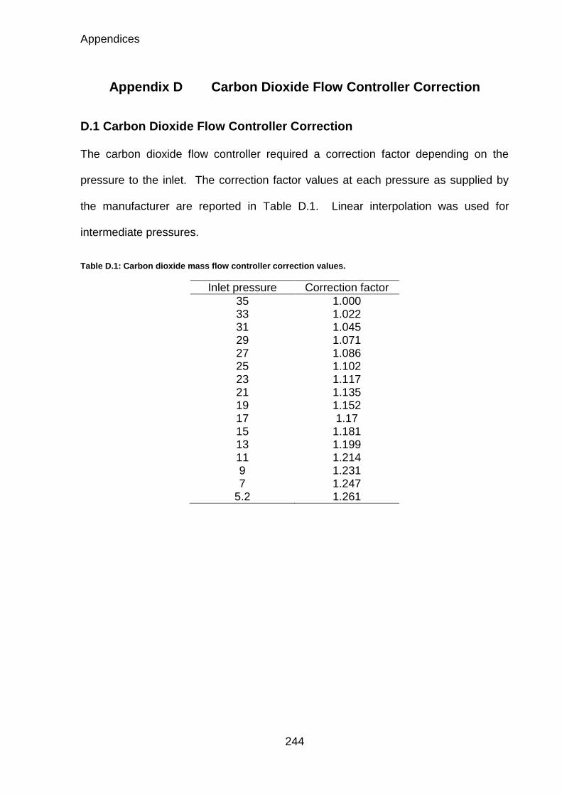
Appendices
244
Appendix D Carbon Dioxide Flow Controller Correction
D.1 Carbon Dioxide Flow Controller Correction
The carbon dioxide flow controller required a correction factor depending on the
pressure to the inlet. The correction factor values at each pressure as supplied by
the manufacturer are reported in Table D.1. Linear interpolation was used for
intermediate pressures.
Table D.1: Carbon dioxide mass flow controller correction values.
Inlet pressure Correction factor
35 1.000 33 1.022 31 1.045 29 1.071 27 1.086 25 1.102 23 1.117 21 1.135 19 1.152 17 1.17 15 1.181 13 1.199 11 1.214 9 1.231 7 1.247
5.2 1.261

Appendices
245
Appendix E Risk Assessment

Appendices
246

Appendices
247

Appendices
248

Appendices
249

Appendices
250
Appendix F gProms Code
The gProms code is split between the 4 main elements, VARAIBLE TYPES,
MODELS, TASKS and PROCESSES. The MODEL defines the equations being
solved and the TASKS define the sequence of the system. This Appendix shows the
code for implementing the equations shown in Chapter 4 in the models. The
implementation of the TASK for the 4 step model described in Section 4.12.1 is also
shown.
F.1 Models
F.1.1 Dispersion Model
PARAMETER
# Number of components
NoComp AS INTEGER
# Bed length, density and cross-sectional area
BedLength AS REAL
# Ideal gas constant
R AS REAL
# Bed Void
BedVoid AS REAL
DISTRIBUTION_DOMAIN
Axial AS [ 0 : BedLength ]
VARIABLE
# Mole Fractions
y AS DISTRIBUTION(NoComp,Axial) OF MoleFraction
yprod AS DISTRIBUTION(NoComp) OF NoType
# Superficial gas velocity
u AS DISTRIBUTION(Axial) OF Velocity
# Volumetric Flow
Q AS DISTRIBUTION(Axial) OF VolumetricFlowrate

Appendices
251
# Pressure
P AS DISTRIBUTION(Axial) OF Pressure
# Temperature
T AS DISTRIBUTION(Axial) OF Temperature
# Feed conditions
Pfeed AS Pressure
Tfeed AS Temperature
yfeed AS ARRAY(NoComp) OF NoType
Qfeed AS Velocity
# Dispersion Coefficient
Dispersion AS Diffusivity
# Bed Properties
BedDiameter AS Length
BedArea AS Area
BOUNDARY
# At the feed end
FOR i := 1 TO NoComp DO
y(i,0) = yfeed(i) ;
END # For
P(0) = Pfeed ;
T(0) = Tfeed ;
u(0) = Qfeed / BedArea / BedVoid ;
# At Bed Exit
PARTIAL(y(,BedLength),Axial) = 0 ;
PARTIAL(u(BedLength),Axial) = 0 ;
EQUATION
# Component mass balance
FOR i := 1 TO NoComp DO
FOR z := 0|+ TO BedLength|- DO
$y(i,z) = -u(z) * PARTIAL(y(i,z) , Axial)
+ Dispersion * PARTIAL(y(i,z) , Axial , Axial);
END # For
END # For
# Overall mass balance
FOR z := 0|+ TO BedLength|- DO
PARTIAL(u(z) , Axial) = 0 ;
END
# Mole Fraction at Bed End
FOR i := 1 to NoComp DO
y(i,BedLength) = yprod(i) ;
END # For
# Isothermal and Isobaric operation
FOR z := 0|+ TO BedLength DO
T(z) = Tfeed ;

Appendices
252
P(z) = Pfeed ;
END # For
# Volumetric Flow
FOR z := 0 TO BedLength DO
Q(z) = u(z) * BedArea * BedVoid ;
END # For
# Bed Area
BedArea = BedDiameter^2 / 4 * 3.141 ;
F.1.2 Adsorption Model
PARAMETER
# Number of components
NoComp AS INTEGER
# Bed Properties
BedLength AS REAL
BedDiameter AS REAL
BedArea AS REAL
BedDensity AS REAL
# Adsorbent Properties
Dp AS REAL
# Ideal gas constant
R AS REAL
# Isotherm Parameters
k11 AS ARRAY(NoComp) OF REAL
k12 AS ARRAY(NoComp) OF REAL
k13 AS ARRAY(NoComp) OF REAL
k14 AS ARRAY(NoComp) OF REAL
k21 AS ARRAY(NoComp) OF REAL
k22 AS ARRAY(NoComp) OF REAL
k23 AS ARRAY(NoComp) OF REAL
k24 AS ARRAY(NoComp) OF REAL
phys_prop AS FOREIGN_OBJECT
# For Dispersion
RMM AS ARRAY(NoComp) OF REAL
visccomp AS ARRAY(NoComp) OF REAL
phi AS ARRAY(NoComp) OF REAL
# For MT
rpore AS REAL
tortuosity AS REAL
Dc_rc2 AS ARRAY(NoComp) OF REAL
DISTRIBUTION_DOMAIN
Axial AS [ 0 : BedLength ]

Appendices
253
UNIT
Diffus AS Diffusivity
EB AS EB_Non_Isothermal_w_wall
VARIABLE
# Assigned Variables
# Feed conditions
Pfeed AS Pressure
Tfeed AS Temperature
Yfeed AS ARRAY(NoComp) OF MoleFraction
Qin AS VolumetricFlowrate
Qfeednorm AS VolumetricFlowrate
Tair AS Temperature
ypress AS ARRAY(NoComp) OF MoleFraction
#Dependent Variables
# Mole fraction
y AS DISTRIBUTION(NoComp,Axial) OF MoleFraction
yfinal AS MoleFraction
# Solid phase concentrations
q AS DISTRIBUTION(NoComp,Axial) OF SolidConcentration
# Equilibrium solid phase concentrations
qeq AS DISTRIBUTION(NoComp,Axial) OF SolidConcentration
# Superficial gas velocity
u AS DISTRIBUTION(Axial) OF Velocity
# Pressure
P AS DISTRIBUTION(Axial) OF Pressure
# Temperature
T AS DISTRIBUTION(Axial) OF Temperature
# Concentration
C AS DISTRIBUTION(Axial) OF NoType
ci AS DISTRIBUTION(NoComp,Axial) OF NoType
density AS DISTRIBUTION(Axial) OF NoType
viscosity AS DISTRIBUTION(Axial) OF NoType
heatcap AS DISTRIBUTION(Axial) OF NoType
thermalcond AS DISTRIBUTION(Axial) OF NoType
Qvol AS DISTRIBUTION(Axial) OF VolumetricFlowrate
# For Parameter Estimation
BedVoid AS NoType
PartVoid AS NoType
TotVoid AS NoType
Dispersion AS Diffusivity
# For Dispersion
Diff AS DISTRIBUTION(Axial) OF Diffusivity
Re AS NoType
Sc AS NoType
Peclet AS NoType

Appendices
254
# For MT
Dk AS ARRAY(NoComp) OF Diffusivity
Dpore AS ARRAY(NoComp) OF Diffusivity
k AS ARRAY(NoComp) OF MassCoefficient
kf AS MassCoefficient
# For Isotherm
qs1 AS DISTRIBUTION(NoComp,Axial) OF NoType
B1 AS DISTRIBUTION(NoComp,Axial) OF NoType
qs2 AS DISTRIBUTION(NoComp,Axial) OF NoType
B2 AS DISTRIBUTION(NoComp,Axial) OF NoType
# For Ergun
A_erg AS NoType
B_erg AS NoType
SET
RMM := [44 , 28] ;
visccomp := [1.82e-5 , 1.53e-5] ;
phi(1) := (1 + (visccomp(1)/visccomp(2))^0.5 *
(RMM(2)/RMM(1))^0.25)^0.5/(8*(1+RMM(1)/RMM(2)))^0.5 ;
phi(2) := (1 + (visccomp(2)/visccomp(1))^0.5 *
(RMM(1)/RMM(2))^0.25)^0.5/(8*(1+RMM(2)/RMM(1)))^0.5 ;
Dc_rc2 := [7.19e-2 , 1.06e-2] ;
rpore := 6.13e-9 ;
tortuosity := 1.414 ;
BOUNDARY
# At the feed end
For i := 1 to NoComp DO
-Dispersion*PARTIAL(y(i,0),Axial) = u(0) * (Yfeed(i) - y(i,0)) ;
END # For
P(0) = Pfeed ;
u(0) = Qin / BedArea / BedVoid ;
- EB.HeatDisp(0) * PARTIAL(T(0),Axial) = phys_prop.VapourDensity(Tfeed,Pfeed,yfeed) *
phys_prop.VapourHeatCapacity(Tfeed,Pfeed,yfeed)/1000 * u(0) * (Tfeed - T(0)) ;
# At the end of the bed
PARTIAL(T(BedLength), Axial) = 0 ;
PARTIAL(P(BedLength), Axial) = 0 ;
PARTIAL(y(,BedLength),Axial) = 0 ;
PARTIAL(u(BedLength),Axial) = 0 ;
EQUATION
# Normalised Flowrate
Qin = Qfeednorm*(1e5*Tfeed/(Pfeed*273))/1e6/60 ;
# Total Voidage
TotVoid = BedVoid + PartVoid - BedVoid*PartVoid ;

Appendices
255
# Component mass balance
FOR i := 1 TO NoComp DO
FOR z := 0|+ TO BedLength|- DO
TotVoid*$y(i,z) = -BedVoid*u(z)*PARTIAL(y(i,z), Axial)
+ BedVoid*Dispersion * (PARTIAL(y(i,z), Axial , Axial) + 2/C(z) * PARTIAL(y(i,z),Axial) *
PARTIAL(C(z), Axial))
- (1-TotVoid) / (C(z)) * ($q(i,z) - y(i,z) * SIGMA($q(,z)));
END # For
END # For
# Overall mass balance
FOR z := 0|+ TO BedLength|- DO
TotVoid*$C(z) = BedVoid*Dispersion*PARTIAL(C(z),Axial,Axial) -
BedVoid*PARTIAL(u(z)*C(z),Axial) - (1-TotVoid) * SIGMA($q(,z)) ;
END # For
FOR z := 0 TO BedLength DO
C(z) = (P(z)/(R*T(z))) ;
END
FOR i := 1 TO NoComp DO
FOR z := 0 TO BedLength DO
ci(i,z)=C(z)*y(i,z) ;
END # For
END # For
# Adsorption rate equation
FOR i := 1 TO NoComp DO
FOR z := 0 TO BedLength DO
$q(i,z) = k(i) * ( (qeq(i,z)) - q(i,z) ) ;
END # For
END # For
# Dual Site Langmuir Isotherm
FOR z := 0 TO BedLength DO
FOR i := 1 TO NoComp DO
qs1(i,z) = k11(i)*exp(k12(i)/(R*T(z))) ;
B1(i,z) = k13(i)*exp(k14(i)/(R*T(z))) ;
qs2(i,z) = k21(i)*exp(k22(i)/(R*T(z))) ;
B2(i,z) = k23(i)*exp(k24(i)/(R*T(z))) ;
qeq(i,z) = BedDensity / (1-TotVoid) * (qs1(i,z)*B1(i,z)*P(z)*y(i,z) / (1 + SIGMA(B1(,z)*P(z)*y(,z)))
+ qs2(i,z)*B2(i,z)*P(z)*y(i,z) / (1 + SIGMA(B2(,z)*P(z)*y(,z)))) ;
END # For
END # For
# Ergun Equation
A_erg = 150 * (1+2*Dp/(3*BedDiameter*(1-BedVoid)))^2 ;
B_erg = 1.75 * (1+2*Dp/(3*BedDiameter*(1-BedVoid))) ;
For z:= 0|+ TO BedLength|- DO
-PARTIAL(P(z), Axial) = A_erg * phys_prop.VapourViscosity(T(z),P(z),y(,z)) * (1 - BedVoid)^2 * u(z) /
(BedVoid^3 * Dp^2)
+ B_erg * (1-BedVoid) / (Dp * BedVoid^3) * u(z) * ABS(u(z)) *
phys_prop.VapourDensity(T(z),P(z),y(,z)) ;
END # For

Appendices
256
# End Mole Fraction
yfinal = y(2,BedLength) ;
FOR z := 0 TO BedLength DO
density(z) = phys_prop.VapourDensity(T(z),P(z),y(,z)) ;
viscosity(z) = phys_prop.VapourViscosity(T(z),P(z),y(,z)) ;
heatcap(z) = phys_prop.VapourHeatCapacity(T(z),P(z),y(,z)) ;
thermalcond(z) = phys_prop.VapourConductivity(T(z),P(z),y(,z)) ;
Qvol(z) = BedArea * u(z) ;
END # For
# Connection to Diff
P() = Diffus.P() ;
T() = Diffus.T() ;
Diff() = Diffus.Diff() ;
# Dispersion
Re = density(BedLength) * u(0) * Dp / viscosity(BedLength) ;
Sc = viscosity(BedLength) / (Diff(0) * density(BedLength)) ;
Peclet = 1/(0.328/(Re*Sc) + 3.33/(1+0.59/(Re*Sc))) ;
Dispersion = u(0) * Dp / Peclet ;
# MT Coeff
kf = Diff(0)/(Dp/2) * (2 + 1.1 * Re^0.6 * Sc^0.33) ;
FOR i := 1 TO NoComp DO
Dk(i) = 9700 * rpore * (Tfeed/RMM(i))^0.5 ;
Dpore(i) = PartVoid * Dk(i) * Diff(0) / (tortuosity * (Dk(i)+Diff(0))) ;
k(i) = 1 / (Dp/2 * qeq(i,0) / (3*kf*ci(i,0)) + (Dp/2)^2*qeq(i,0) / (15*PartVoid*Dpore(i)*ci(i,0)) + 1 /
15/Dc_rc2(i)) ;
END # For
# Connection to EB
T = EB.T ;
Tfeed = EB.Tfeed ;
Tair = EB.Tair ;
u = EB.u ;
q = EB.q ;
y = EB.y ;
P = EB.P ;
Re = EB.Re ;
BedVoid = EB.BedVoid ;
TotVoid = EB.TotVoid ;
F.1.3 Diffusivity Model
PARAMETER
NoComp AS INTEGER
BedLength AS REAL
RMM AS ARRAY(NoComp) OF REAL
sig AS ARRAY(NoComp) OF REAL
sigmix AS REAL
EpsoKap AS ARRAY(NoComp) OF REAL
EpsoKapmix AS REAL
Omega AS REAL
DISTRIBUTION_DOMAIN
Axial AS [ 0 : BedLength ]

Appendices
257
VARIABLE
P AS DISTRIBUTION(Axial) OF Pressure
T AS DISTRIBUTION(Axial) OF Temperature
Tdim AS DISTRIBUTION(Axial) OF Temperature
Diff AS DISTRIBUTION(Axial) OF Diffusivity
SET
RMM := [44 , 28] ;
sig := [3.996 , 3.617] ;
sigmix := 0.5 * SIGMA(sig()) ;
EpsoKap := [190 , 97] ;
EpsoKapmix := PRODUCT(EpsoKap())^0.5 ;
Omega := 1.042 ;
EQUATION
FOR z := 0 TO BedLength DO
Tdim(z) = T(z)/ EpsoKapmix ;
Diff(z) = (0.0018583*(T(z)^3*(1/RMM(1)+1/RMM(2)))^0.5 / (P(z)/1e5*sigmix^2*Omega))/1e4 ;
END # For
F.1.4 Energy Balance Model
PARAMETER
# Number of Components
NoComp AS INTEGER
# Bed Properties
BedLength AS REAL
BedDiameter AS REAL
BedArea AS REAL
BedDensity AS REAL
# Adsorbent Properties
Dp AS REAL
# Heat transfer coefficients
HeatCapacityPart AS REAL
HeatAdsorp AS ARRAY(NoComp) OF REAL
HeatTranStag AS REAL
alphaw AS REAL
# Ideal gas constant
R AS REAL
# Physical Properties
phys_prop AS FOREIGN_OBJECT
DISTRIBUTION_DOMAIN
Axial AS [ 0 : BedLength ]
VARIABLE
# Temperature

Appendices
258
T AS DISTRIBUTION(Axial) OF Temperature
Tfeed AS Temperature
Tair AS Temperature
# Superficial Velocity
u AS DISTRIBUTION(Axial) OF Velocity
# Solid Phase Concentration
q AS DISTRIBUTION(NoComp,Axial) OF SolidConcentration
# Pressure
P AS DISTRIBUTION(Axial) OF Pressure
# Mole Fraction
y AS DISTRIBUTION(NoComp,Axial) OF MoleFraction
# BedVoid
BedVoid AS NoType
TotVoid AS NoType
# Calcing HTCoeffWall
HTCoeffWall AS DISTRIBUTION(Axial) OF NoType
Pr AS DISTRIBUTION(Axial) OF NoType
Re AS DISTRIBUTION(Axial) OF NoType
PrRe AS DISTRIBUTION(Axial) OF Dimensionless
HeatDisp AS DISTRIBUTION(Axial) OF NoType
yagi AS DISTRIBUTION(Axial) OF NoType
EQUATION
# HT Coeff Wall
FOR z := 0 TO BedLength DO
Pr(z) = phys_prop.VapourHeatCapacity(T(z),P(z),y(,z))*phys_prop.VapourViscosity(T(z),P(z),y(,z))/
phys_prop.VapourConductivity(T(z),P(z),y(,z)) ;
PrRe(z) = 2.19*(Pr(z) * Re(z))^(1/3) ;
HTCoeffWall(z) = yagi(z) ;
yagi(z) = HeatTranStag + alphaw * phys_prop.VapourHeatCapacity(T(z),P(z),y(,z))/1000 *
phys_prop.VapourDensity(T(z),P(z),y(,z)) * u(z) ;
HeatDisp(z) = phys_prop.VapourConductivity(T(z),P(z),y(,z))*(7+0.5*Pr(z)*Re(z))/1000;
END # For
# Non-Isothermal
FOR z := 0|+ TO BedLength|- DO
(TotVoid * phys_prop.VapourDensity(T(z),P(z),y(,z)) *
phys_prop.VapourHeatCapacity(T(z),P(z),y(,z))/1000 + BedDensity * HeatCapacityPart) * $T(z) =
- phys_prop.VapourDensity(T(z),P(z),y(,z)) * phys_prop.VapourHeatCapacity(T(z),P(z),y(,z))/1000 *
BedVoid * PARTIAL(T(z) *u(z)/BedVoid ,Axial)
+ HeatDisp(z) * PARTIAL(T(z),Axial,Axial)
+ (1 - TotVoid) * SIGMA(HeatAdsorp()*$q(,z))
- 4 * HTCoeffWall(z) / BedDiameter * (T(z) - Tair) ;
END # For

Appendices
259
F.2 Tasks
F.2.1 4 Step Skarstrom Cycle
PARAMETER
Column AS MODEL Whole_System_Full
SCHEDULE
SEQUENCE
CONTINUE FOR Column.ad_time
REASSIGN
WITHIN Column DO
yfeedsys := ypurge ;
END
END
SWITCH
Column.Press_set := Column.deflow ;
END
CONTINUE UNTIL Column.Qfeednormsys <= Column.Qblow_1
SWITCH
Column.Press_set := Column.Depress ;
END
REASSIGN
Column.deflowrate := Column.deflowRate_2 ;
END # Reassign
CONTINUE UNTIL Column.Qoutmole >= Column.Depress_outmole
WHILE Column.Pfeedsys >= Column.Plow DO
SEQUENCE
REASSIGN
Column.error_de := -OLD(Column.Qoutmole)+Column.Depress_outmole ;
Column.DepressRate := OLD(Column.DepressRate)*
(OLD(Column.error_de)*Column.Depress_prop+1) ;
END # Reassign
CONTINUE FOR 0.1
END # Sequence
END # While
REASSIGN
Column.DepressRate := Column.DepressRateInt ;
Column.error_de := Column.Error_de_int ;
END # Reassign
SWITCH
Column.Press_set := Column.deflow ;
END
CONTINUE UNTIL Column.Qfeednormsys <= Column.Qblow_2
SWITCH
Column.Press_set := Column.Con ;
END

Appendices
260
CONTINUE FOR Column.blow_time
SWITCH
Column.Press_set := Column.reflow ;
END
CONTINUE UNTIL Column.Qfeednormsys >= Column.Qpurge
SWITCH
Column.Press_set := Column.Con ;
END
CONTINUE FOR Column.purge_time
END # Sequence

Appendices
261
Appendix G Compressibility Factor Calculation
G.1 Compressibility Factor Calculation
The cubic equation of state is often used to account for the deviation from the ideal
gas law, with a two parameter cubic equation shown by Equation G.1.1.
P =𝑅𝑇
𝑉 − 𝑏−
𝑎
𝑉2 + 𝑢𝑏𝑉 + 𝑤𝑏2 G.1.1
Another form of Equation G.1.1 is shown by Equation G.1.2 based on
compressibility. (Reid et al., 1987)
𝑍3 − (1 + 𝐵∗ − 𝑢𝐵∗)𝑍2 + (𝐴∗ + 𝑤𝐵∗ − 𝑢𝐵∗ − 𝑢𝐵∗2)𝑍 − 𝐴∗𝐵∗ − 𝑤𝐵∗2
− 𝑤𝐵∗3 = 0 G.1.2
𝐴∗ =𝑎𝑃
𝑅2𝑇2 G.1.3
𝐵∗ =𝑏𝑃
𝑅𝑇 G.1.4
There are several equation of states used for predicting the values of 𝑢, 𝑤, 𝑎 and 𝑏
The Peng-Robinson equation has previously been applied to high pressure
adsorption systems by Casas et al. (2012). For the Peng-Robinson equation of state
the value for 𝑢 is 2 and the value for 𝑤 is -1. The pure component values for 𝑎 and 𝑏
are given by Equations G.1.5 and G.1.6 respectively.
a =0.45724𝑅2𝑇𝑐
2
𝑃𝑐[1 + fω(1 − 𝑇𝑟
1 2⁄ )]2 G.1.5
b =0.07780𝑅𝑇𝑐
𝑃𝑐 G.1.6
fω = 0.37464 + 1.54266ω − 0.26992𝜔2 G.1.7

Appendices
262
For gas mixtures the proportion of the constants 𝑎 and 𝑏 need to be found using
Equations G.1.8 and G.1.9 respectively. The value of 𝑘𝑖𝑗̅̅ ̅̅ for a CO2/N2 mixture using
the Peng-Robinson equation is -0.017.
a𝑚 =∑∑𝑦𝑖𝑦𝑗(𝑎𝑖𝑎𝑗)1/2(1 − 𝑘𝑖𝑗̅̅ ̅̅ )
𝑗𝑖
G.1.8
b𝑚 =∑𝑦𝑖𝑏𝑖𝑖
G.1.9
The properties used in the calculation of the compressibility for CO2/N2 mixtures are
given in Table G.1. The range of compressibility factors calculated for the gas
mixtures simulated in this study are reported in Table G.2.
Table G.1: Carbon dioxide and nitrogen properties for the calculation of compressibility. (Reid et al., 1987)
Carbon Dioxide Nitrogen
𝑇𝑐 (K) 304.1 126.2
𝑃𝑐 (bar) 73.8 33.9
ω (-) 0.239 0.039
T (K) 298 298
P (bar) 25 25
Table G.2: CO2/N2 mixture compressibility factors for the range of carbon dioxide feed fractions studied.
CO2 Mole Fraction Z (-)
0 0.958 0.1 0.951 0.2 0.943 0.3 0.934 0.4 0.925 0.5 0.915

Appendices
263
Table G.3: Nomenclature used in Appendix G.
𝐴∗ Condition constant used in cubic equation of state
a Condition constant used in cubic equation of state
a𝑚 Condition constant used in cubic equation of state for gas mixtures
𝐵∗ Condition constant used in cubic equation of state
𝑏 Condition constant used in cubic equation of state
b𝑚 Condition constant used in cubic equation of state for gas mixtures
fω Condition constant used in cubic equation of state
𝑘𝑖𝑗̅̅ ̅̅ Condition constant used in cubic equation of state for gas mixtures
𝑃 Pressure
P𝑐 Critical pressure
𝑅 Gas constant
𝑇 Temperature
T𝑐 Critical Temperature
T𝑟 Relative Temperature
𝑢 Condition constant used in cubic equation of state
𝑉 Gas volume
𝑤 Condition constant used in cubic equation of state
𝑦 Component mole fraction
𝑍 Compressibility factor
ω Pitzer’s acentric factor

Appendices
264
Appendix H Component Mass Balance Derivation
H.1 Component Mass Balance Derivation
The general component mass balance is given by Equation H.1.1.
휀𝑡𝜕𝑐𝑖𝜕𝑡= −휀𝑏
𝜕(𝑐𝑖𝑣)
𝜕𝑧+ 휀𝑏𝐷𝑎𝑥
𝜕2𝑐𝑖𝜕𝑧2
− 𝜌𝑏𝜕𝑞𝑖𝜕𝑡
H.1.1
It is possible to represent the component concentration as a product of the total
concentration and the component mole fraction in Equation H.1.2 and then expanded
to give Equation H.1.4.
휀𝑡𝜕(𝐶𝑦𝑖)
𝜕𝑡= −휀𝑏
𝜕(𝐶𝑦𝑖𝑣)
𝜕𝑧+ 휀𝑏𝐷𝑎𝑥
𝜕2(𝐶𝑦𝑖)
𝜕𝑧2− 𝜌𝑏
𝜕𝑞𝑖𝜕𝑡
H.1.2
휀𝑡 (𝐶𝜕𝑦𝑖𝜕𝑡+ 𝑦𝑖
𝜕𝐶
𝜕𝑡)
= −휀𝑏 (𝐶𝑣𝜕𝑦𝑖𝜕𝑧+ 𝑦𝑖
𝜕(𝐶𝑣)
𝜕𝑧) + 휀𝑏𝐷𝑎𝑥 (
𝜕
𝜕𝑧(𝐶𝜕𝑦𝑖𝜕𝑧+ 𝑦𝑖
𝜕𝐶
𝜕𝑧))
− 𝜌𝑏𝜕𝑞𝑖𝜕𝑡
H.1.3
휀𝑡 (𝐶𝜕𝑦𝑖𝜕𝑡+ 𝑦𝑖
𝜕𝐶
𝜕𝑡)
= −휀𝑏 (𝐶𝑣𝜕𝑦𝑖𝜕𝑧+ 𝑦𝑖
𝜕(𝐶𝑣)
𝜕𝑧)
+ 휀𝑏𝐷𝑎𝑥 (𝐶𝜕2𝑦𝑖𝜕𝑧2
+ 2𝜕𝑦𝑖𝜕𝑧
𝜕𝐶
𝜕𝑧+ 𝑦𝑖
𝜕2𝐶
𝜕𝑧2) − 𝜌𝑏
𝜕𝑞𝑖𝜕𝑡
H.1.4
The overall mass balance is given by Equation H.1.5 and multiplied by the
component mole fraction to given Equation H.1.6.
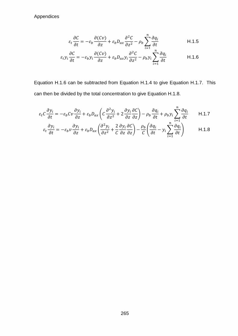
Appendices
265
휀𝑡𝜕𝐶
𝜕𝑡= −휀𝑏
𝜕(𝐶𝑣)
𝜕𝑧+ 휀𝑏𝐷𝑎𝑥
𝜕2𝐶
𝜕𝑧2− 𝜌𝑏∑
𝜕𝑞𝑖𝜕𝑡
𝑛
𝑖=1
H.1.5
휀𝑡𝑦𝑖𝜕𝐶
𝜕𝑡= −휀𝑏𝑦𝑖
𝜕(𝐶𝑣)
𝜕𝑧+ 휀𝑏𝐷𝑎𝑥𝑦𝑖
𝜕2𝐶
𝜕𝑧2− 𝜌𝑏𝑦𝑖∑
𝜕𝑞𝑖𝜕𝑡
𝑛
𝑖=1
H.1.6
Equation H.1.6 can be subtracted from Equation H.1.4 to give Equation H.1.7. This
can then be divided by the total concentration to give Equation H.1.8.
휀𝑡𝐶𝜕𝑦𝑖𝜕𝑡= −휀𝑏𝐶𝑣
𝜕𝑦𝑖𝜕𝑧+ 휀𝑏𝐷𝑎𝑥 (𝐶
𝜕2𝑦𝑖𝜕𝑧2
+ 2𝜕𝑦𝑖𝜕𝑧
𝜕𝐶
𝜕𝑧) − 𝜌𝑏
𝜕𝑞𝑖𝜕𝑡+ 𝜌𝑏𝑦𝑖∑
𝜕𝑞𝑖𝜕𝑡
𝑛
𝑖=1
H.1.7
휀𝑡𝜕𝑦𝑖𝜕𝑡= −휀𝑏𝑣
𝜕𝑦𝑖𝜕𝑧+ 휀𝑏𝐷𝑎𝑥 (
𝜕2𝑦𝑖𝜕𝑧2
+2
𝐶
𝜕𝑦𝑖𝜕𝑧
𝜕𝐶
𝜕𝑧) −
𝜌𝑏𝐶(𝜕𝑞𝑖𝜕𝑡− 𝑦𝑖∑
𝜕𝑞𝑖𝜕𝑡
𝑛
𝑖=1
) H.1.8
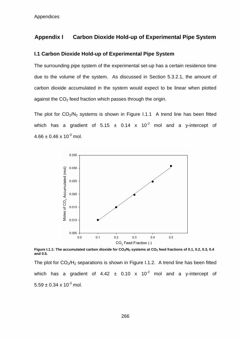
Appendices
266
Appendix I Carbon Dioxide Hold-up of Experimental Pipe System
I.1 Carbon Dioxide Hold-up of Experimental Pipe System
The surrounding pipe system of the experimental set-up has a certain residence time
due to the volume of the system. As discussed in Section 5.3.2.1, the amount of
carbon dioxide accumulated in the system would expect to be linear when plotted
against the CO2 feed fraction which passes through the origin.
The plot for CO2/N2 systems is shown in Figure I.1.1 A trend line has been fitted
which has a gradient of 5.15 ± 0.14 x 10⁻² mol and a y-intercept of
4.66 ± 0.46 x 10⁻³ mol.
Figure I.1.1: The accumulated carbon dioxide for CO2/N2 systems at CO2 feed fractions of 0.1, 0.2, 0.3, 0.4 and 0.5.
The plot for CO2/H2 separations is shown in Figure I.1.2. A trend line has been fitted
which has a gradient of 4.42 ± 0.10 x 10⁻² mol and a y-intercept of
5.59 ± 0.34 x 10⁻³ mol.

Appendices
267
Figure I.1.2: The accumulated carbon dioxide for CO2/H2 systems at CO2 feed fractions of 0.1, 0.2, 0.3, 0.4 and 0.5.

Appendices
268
Appendix J Dispersion and Mass Transfer Coefficient
Calculation
J.1 Dispersion Coefficient
The dispersion coefficient can be predicted from a range correlations which calculate
the Peclet number, the dimensionless group used in the evaluation of the dispersion
coefficient. The Reynolds number is the ratio of inertial and viscous forces and the
Schmidt number is the ratio of viscous and diffusive properties (Bird et al., 2001).
The sum of the Reynolds’ and Schmidt number is used for finding the Peclet number.
The two dimensionless groups are:
𝑅𝑒 =𝜌𝑢𝑑𝑝
𝜇 𝑎𝑛𝑑 𝑆𝑐 =
𝜇
𝜌𝐷𝐴𝐵
These are both affected by the viscosity of the gas and the gas density, however,
when the number are multiplied together the two properties cancel out making the
system only dependent on the particle diameter, the gas velocity and the gas
diffusivity. The particle diameter is 1 mm and the gas velocity is 7.41 X 10⁻⁴ m s-1 for
all CO2 feed fractions. The gas diffusivity for a CO2/N2 mixture is 6.12 x 10⁻⁷ m2 s-1
and 2.22 x 10⁻⁶ m2 s-1 for a CO2/H2 mixture. The dispersion coefficient can be
calculated by the Wakao and Funazkri (1978) correlation, the general correlation
given in Ruthven (1984) and the Hsu and Haynes (1981) correlation, all shown in
Section 4.7.1. The calculated dispersion coefficients from these three correlations for
each of the system studied are presented in Table J.1.

Appendices
269
Table J.1: Dispersion coefficient calculated from three correlations for all system studied here.
Diffusivity Wakao General Hsu and Haynes
(m2 s-1) Pe Dax (m2 s-1) Pe Dax (m
2 s-1) Pe Dax (m2 s-1)
CO2/N2 AC 6.12 x 10⁻⁷ 0.103 6.03 x 10⁻⁶ 0.906 6.82 x 10⁻⁷ 0.412 1.50 x 10⁻⁶
CO2/N2 MAC 2.22 x 10⁻⁶ 0.059 1.26 x 10⁻⁵ 0.975 7.61 x 10⁻⁷ 0.398 1.86 x 10⁻⁶
CO2/H2 MAC 6.12 x 10⁻⁷ 0.017 4.48 x 10⁻⁵ 0.415 1.79 x 10⁻⁶ 0.457 1.62 x 10⁻⁶
J.2 Mass Transfer Coefficient
The mass transfer coefficient which incorporates the surface, macropore and
micropore mass transfer resistances can be calculated by a correlation presented by
Farooq and Ruthven (1990). These correlations for the parameters describing the
mass transfer resistance are reported in Section 4.7.2. Each individual resistance
can be calculated from the respective part of the correlation as each resistance is
assumed to be additive, as shown by Equations J.2.1 to J.2.3.
1
𝑘𝑠𝑢𝑟𝑓𝑎𝑐𝑒,𝑖=𝑑𝑝𝑞0,𝑖
6𝑘𝑓𝑐0,𝑖
J.2.1
1
𝑘𝑚𝑎𝑐𝑟𝑜𝑝𝑜𝑟𝑒,𝑖=
𝑑𝑝𝑜𝑟𝑒2 𝑞0,𝑖
60휀𝑝𝐷𝑝𝑜𝑟𝑒𝑐0,𝑖 J.2.2
1
𝑘𝑚𝑖𝑐𝑟𝑜𝑝𝑜𝑟𝑒,𝑖=
𝑟𝑐2
15𝐷𝑐 J.2.3
These can be calculated for all three systems studied here as shown in Table J.2.
The values for hydrogen using the modified activated carbon are not presented as
hydrogen is assumed to not adsorb on the system. Calculating values for hydrogen
being adsorbed would require the hydrogen isotherm. The carbon dioxide isotherm
data for this separation is based on pure component data.

Appendices
270
Table J.2: Mass transfer resistances for all systems studied.
AC – CO2/N2 MAC – CO2/N2 MAC – CO2/H2*
CO2 N2 CO2 N2 CO2 H2
𝑘𝑠𝑢𝑟𝑓𝑎𝑐𝑒,𝑖 (s-1) 0.67 8.60 0.41 37.5 1.27 -
𝑘𝑚𝑎𝑐𝑟𝑜𝑝𝑜𝑟𝑒,𝑖 (s-1) 0.43 5.47 0.31 28.2 1.07 -
𝑘𝑚𝑖𝑐𝑟𝑜𝑝𝑜𝑟𝑒,𝑖 (s-1) 0.16 1.08 0.16 1.08 0.16 -
𝑘𝑖 (s-1) 0.099 0.81 0.083 1.01 0.12 1.08
*All values found assume that no hydrogen is adsorbed and the carbon dioxide
adsorbed amount is based on a pure component isotherm.

Appendices
271
Appendix K System Model Parameters
K.1 System Model Parameters
Figure K.1.1: Model configuration for the simulation of the system without a bed
The system without the bed, described in Section 3.6.2, was fitted to experimental
data using a configuration of beds, as shown in Figure K.1.1, with each bed based on
the reduced axial dispersed plug flow model. Beds 1 and 2 were matched to the
analyser response and the same parameters were used for all carbon dioxide mole
fraction. The bed lengths were found through iteration to match the breakthrough
time. The bed area and dispersion coefficient were found using the gProms
parameter estimation tool. Beds 3 and 4 were matched to the response of the
analyser to the experiments for the system without the bed. The bed lengths were
found through iteration to match the breakthrough time and were kept constant for all
carbon dioxide mole fractions. The bed area and dispersion coefficient were found
using the gProms parameter estimation tool individually for each carbon dioxide feed
fraction. The parameters for all four beds are shown in Table K.1.

Appendices
272
Table K.1: Parameters used for the simulation of the system without a bed
0.1 0.2 0.3 0.4 0.5
Bed 1
Bed Length (m) 0.002 0.002 0.002 0.002 0.002 Bed Area (m2) 1.25 x 10⁻³ 1.25 x 10⁻³ 1.25 x 10⁻³ 1.25 x 10⁻³ 1.25 x 10⁻³ Dispersion (m2 s-1) 4.14 x 10⁻⁹ 4.14 x 10⁻⁹ 4.14 x 10⁻⁹ 4.14 x 10⁻⁹ 4.14 x 10⁻⁹
Bed 2
Bed Length (m) 1 1 1 1 1 Bed Area (m2) 1.05 x 10⁻⁴ 1.05 x 10⁻⁴ 1.05 x 10⁻⁴ 1.05 x 10⁻⁴ 1.05 x 10⁻⁴ Dispersion (m2 s-1) 1.21 x 10⁻² 1.21 x 10⁻² 1.21 x 10⁻² 1.21 x 10⁻² 1.21 x 10⁻²
Bed 3
Bed Length (m) 5.5 5.5 5.5 5.5 5.5 Bed Area (m2) 9.39 x 10⁻⁶ 6.50 x 10⁻⁶ 3.98 x 10⁻⁶ 3.15 x 10⁻⁶ 3.00 x 10⁻⁶ Dispersion (m2 s-1) 9.14 x 10⁻³ 4.61 x 10⁻³ 1.32 x 10⁻³ 1.20 x 10⁻³ 1.41 x 10⁻³
Bed 4
Bed Length (m) 4.5 4.5 4.5 4.5 4.5 Bed Area (m2) 9.47 x 10⁻⁶ 7.27 x 10⁻⁶ 7.56 x 10⁻⁶ 7.89 x 10⁻⁶ 7.44 x 10⁻⁶ Dispersion (m2 s-1) 1.82 x 10⁻⁴ 6.06 x 10⁻⁵ 9.61 x 10⁻⁵ 3.98 x 10⁻⁵ 1.84 x 10⁻⁵

List of References
273
List of References
Agarwal, A., Biegler, L.T., Zitney, S.E., 2010. Superstructure-Based Optimal Synthesis of Pressure Swing Adsorption Cycles for Precombustion CO2 Capture. Industrial & Engineering Chemistry Research 49, 5066-5079.
Ahn, H., Lee, C.-H., Seo, B., Yang, J., Baek, K., 1999. Backfill Cycle of a Layered Bed H2 PSA Process. Adsorption 5, 419-433.
Bell, D.A., Towler, B.F., 2010. Coal gasification and its applications. Elsevier Science, Oxford.
Bird, R.B., Stewart, W.E., Lightfoot, E.N., 2001. Transport Phenomena, 2nd ed. John Wiley & Sons, Inc., Chichester.
Bottani, E.J., Tascon, J.M.D., 2008. Adsorption by carbons. Elsevier, London.
BP, 2014. BP Statistical Review of World Energy 2014, London.
Casas, N., Schell, J., Blom, R., Mazzotti, M., 2013a. MOF and UiO-67/MCM-41 adsorbents for pre-combustion CO2 capture by PSA: Breakthrough experiments and process design. Separation and Purification Technology 112, 34-48.
Casas, N., Schell, J., Joss, L., Mazzotti, M., 2013b. A parametric study of a PSA process for pre-combustion CO2 capture. Separation and Purification Technology 104, 183-192.
Casas, N., Schell, J., Pini, R., Mazzotti, M., 2012. Fixed bed adsorption of CO2/H-2 mixtures on activated carbon: experiments and modeling. Adsorption-Journal of the International Adsorption Society 18, 143-161.
Cavenati, S., Grande, C.A., Rodrigues, A.E., 2006. Separation of mixtures by layered pressure swing adsorption for upgrade of natural gas. Chemical Engineering Science 61, 3893-3906.
Cen, P.-L., Chen, W.-N., Yang, R.T., 1985. Ternary Gas Mixture Separation by Prssure Swing Adsorption: A Combined Hydrogen-Methane Seaparation and Acid Gas Removal Process. Industrial Engineering Chemical Process Design and Development 24, 1201-1208.
Cen, P.-L., Yang, R.T., 1986. Bulk Gas Separation by Pressure Swing Adsorption. Industrial Engineering Chemical Fundamentals 25, 758-767.
Chen, C., Rubin, E.S., 2009. CO2 control technology effects on IGCC plant performance and cost. Energy Policy 37, 915-924.
Chen, Z., Deng, S., Wei, H., Wang, B., Huang, J., Yu, G., 2013. Activated carbons and amine-modified materials for carbon dioxide capture — a review. Frontiers of Environmental Science & Engineering 7, 326-340.
Chiesa, P., Consonni, S., Kreutz, T., Williams, R., 2005. Co-production of hydrogen, electricity and CO2 from coal with commercially ready technology.

List of References
274
Part A: Performance and emissions. International Journal of Hydrogen Energy 30, 747-767.
Choi, B.-U., Nam, G.-M., Choi, D.-K., Lee, B.-K., Kim, S.-H., Lee, C.-H., 2004. Adsorption and regeneration dynamic characteristics of methane and hydrogen binary system. Korean Journal of Chemical Engineering 21, 821-828.
Choi, C.-T., Wen-Chung, H., 1994. Incorporation of a valve equation into the simulation of a pressure swing adsorption process. Chemical Engineering Science 49, 75-84.
Choi, W.-K., Kwon, T.-I., Yeo, Y.-K., Lee, H., Song, H., Na, B.-K., 2003. Optimal operation of the pressure swing adsorption (PSA) process for CO2 recovery. Korean Journal of Chemical Engineering 20, 617-623.
Chou, C.-T., Chen, C.-Y., 2004. Carbon dioxide recovery by vacuum swing adsorption. Separation and Purification Technology 39, 51-65.
Chue, K.T., Kim, J.N., Yoo, Y.J., Cho, S.H., Yang, R.T., 1995. Comparison of Activated Carbon and Zeolite 13X for CO2 Recovery from Flue Gas by Pressure Swing Adsorption. Industrial & Engineering Chemistry Research 34, 591-598.
Committee on Climate Change, 2010a. The Fourth Carbon Budget: Reducing Emissions Through the 2020s, London.
Committee on Climate Change, 2010b. Meeting Carbon Budgets - Ensuring a low-carbon recovery: 2nd report to Parliament, London.
Danckwerts, P.V., 1953. Continuous flow systems: Distribution of residence times. Chemical Engineering Science 2, 1-13.
Dantas, T.L.P., Luna, F.M.T., Silva Jr, I.J., de Azevedo, D.C.S., Grande, C.A., Rodrigues, A.E., Moreira, R.F.P.M., 2011. Carbon dioxide–nitrogen separation through adsorption on activated carbon in a fixed bed. Chemical Engineering Journal 169, 11-19.
Delgado, J.A., Rodrigues, A.E., 2008. Analysis of the boundary conditions for the simulation of the pressure equalization step in PSA cycles. Chemical Engineering Science 63, 4452-4463.
Delgado, J.A., Uguina, M.A., Sotelo, J.L., Águeda, V.I., Sanz, A., Gómez, P., 2011. Numerical analysis of CO2 concentration and recovery from flue gas by a novel vacuum swing adsorption cycle. Computers & Chemical Engineering 35, 1010-1019.
Delgado, J.A., Uguina, M.A., Sotelo, J.L., Ruíz, B., 2006. Fixed-bed adsorption of carbon dioxide-helium, nitrogen-helium and carbon dioxide-nitrogen mixtures onto silicalite pellets. Separation and Purification Technology 49, 91-100.

List of References
275
Descamps, C., Bouallou, C., Kanniche, M., 2008. Efficiency of an Integrated Gasification Combined Cycle (IGCC) power plant including CO2 removal. Energy 33, 874-881.
Do, D.D., 1998. Adsorption Analysis: Equilibria and Kinetics. Imperial College Press, London.
Doong, S.J., Yang, R.T., 1986. Bulk Separation of Multicomponent Gas Mixtrues by Pressure Swing Adsorption: Pore/Surface Diffusion and Equilibrium Models. AIChE Journal 32, 397-410.
Doong, S.J., Yang, R.T., 1987a. Bidisperse Pore Diffusion Model for Zeolite Pressure Swing Adsorption. AIChE Journal 33, 1045-1049.
Doong, S.J., Yang, R.T., 1987b. Hydrogen Purification by the Multibed Pressure Swing Adsorption Process. Reactive Polymers 6, 7-13.
Drage, T.C., Blackman, J.M., Pevida, C., Snape, C.E., 2009a. Evaluation of Activated Carbon Adsorbents for CO2 Capture in Gasification. Energy & Fuels 23, 2790-2796.
Drage, T.C., Kozynchenko, O., Pevida, C., Plaza, M.G., Rubiera, F., Pis, J.J., Snape, C.E., Tennison, S., 2009b. Developing activated carbon adsorbents for pre-combustion CO2 capture. Energy Procedia 1, 599-605.
Dreisbach, F., Staudt, R., Keller, J.U., 1999. High Pressure Adsorption Data of Methane, Nitrogen, Carbon Dioxide and their Binary and Ternary Mixtures on Activated Carbon. Adsorption 5, 215-227.
Dullen, F.A.L., 1979. Porous Media: Fluid Transport and Pore Structure. Academic Press, London.
European Commission - Joint Research Centre (JRC)/PBL Netherlands Environmental Assessment Agency, 2011. Emission Database for Global Atmospheric Research (EDGAR), release version 4.2 ed.
Farooq, S., Ruthven, D.M., 1990. Heat effects in adsorption column dynamics. 2. Experimental validation of the one-dimensional model. Industrial & Engineering Chemistry Research 29, 1084-1090.
Figueroa, J., Fout, T., Plasynski, S., McIlvried, H., Srivastava, R.D., 2008. Advances in CO2 capture technology-The U.S. Department of Energy's Carbon Sequestration Program. International Journal of Greenhouse Gas Control 2, 9-20.
Gao, F., Zhou, J., Bian, Z., Jing, C., Hu, J., Liu, H., 2013. Dynamic properties in CO2 adsorption on amine-modified MCM-41. Proceedings of the Institution of Mechanical Engineers, Part E: Journal of Process Mechanical Engineering 227, 106-116.
Gao, W., Butler, D., Tomasko, D.L., 2004. High-Pressure Adsorption of CO2 on NaY Zeolite and Model Prediction of Adsorption Isotherms. Langmuir 20, 8083-8089.

List of References
276
García, S., Gil, M.V., Martín, C.F., Pis, J.J., Rubiera, F., Pevida, C., 2011. Breakthrough adsorption study of a commercial activated carbon for pre-combustion CO2 capture. Chemical Engineering Journal 171, 549-556.
García, S., Pis, J.J., Rubiera, F., Pevida, C., 2013. Predicting Mixed-Gas Adsorption Equilibria on Activated Carbon for Precombustion CO2 Capture. Langmuir 29, 6042-6052.
Garg, D.R., Ruthven, D.M., 1975. Performance of molecular sieve adsorption columns: combined effects of mass transfer and longitudinal diffusion. Chemical Engineering Science 30, 1192-1194.
Global CCS Institute, 2013. The Global Status of CCS: 2013, Canberra, Australia.
Glueckauf, E., Coates, J.I., 1947. 241. Theory of chromatography. Part IV. The influence of incomplete equilibrium on the front boundary of chromatograms and on the effectiveness of separation. Journal of the Chemical Society (Resumed), 1315-1321.
Gomes, V.G., Yee, K.W.K., 2002. Pressure swing adsorption for carbon dioxide sequestration from exhaust gases. Separation and Purification Technology 28, 161-171.
Grande, C.A., 2012. Advances in Pressure Swing Adsorption for Gas Separation. ISRN Chemical Engineering 2012, 13.
Grande, C.A., Blom, R., Möller, A., Möllmer, J., 2013. High-pressure separation of CH4/CO2 using activated carbon. Chemical Engineering Science 89, 10-20.
Gregg, S.J., Sing, K.S.W., 1991. Adsorption, surface area, and porosity. Academic Press.
Himeno, S., Komatsu, T., Fujita, S., 2005. High-Pressure Adsorption Eqeuilbria of Methane and Carbon Dioxide on Several Activated Carbons. Journal of Chemical Engineering Data 50, 369-376.
Hsu, L.K.P., Haynes, H.W., 1981. Effective diffusivity by the gas chromatography technique: Analysis and application to measurements of diffusion of various hydrocarbons in zeolite NaY. AIChE Journal 27, 81-91.
IEA, 2012. Energy technology perspectives: Pathways to a clean energy system, France.
Kikkinides, E.S., Yang, R.T., Cho, S.H., 1993. Concentration and recovery of carbon dioxide from flue gas by pressure swing adsorption. Industrial & Engineering Chemistry Research 32, 2714-2720.
Ko, D., Siriwardane, R., Biegler, L.T., 2002. Optimization of a Pressure-Swing Adsorption Process Using Zeolite 13X for CO2 Sequestration. Industrial & Engineering Chemistry Research 42, 339-348.

List of References
277
Ko, D., Siriwardane, R., Biegler, L.T., 2005. Optimization of Pressure Swing Adsorption and Fractionated Vacuum Pressure Swing Adsorption Processes for CO2 Capture. Industrial & Engineering Chemistry Research 44, 8084-8094.
Krishnan, G., Steele, D., O'Brien, K., Callahan, R., Berchtold, K., Figueroa, J., 2009. Simulation of a Process to Capture CO2 From IGCC Syngas Using a High Temperature PBI Membrane. Energy Procedia 1, 4079-4088.
Kunze, C., Spliethoff, H., 2010. Modelling of an IGCC plant with carbon capture for 2020. Fuel Processing Technology 91, 934-941.
Langmuir, I., 1918. THE ADSORPTION OF GASES ON PLANE SURFACES OF GLASS, MICA AND PLATINUM. Journal of the American Chemical Society 40, 1361-1403.
Leva, M., 1947. Heat Transfer to Gases through Packed Tubes. Industrial & Engineering Chemistry 39, 857-862.
LeVaque, R.J., 2007. Finite Difference Methods for Ordinary and Partial Differential Equations. Society for Industrial and Applied Mathematics, Philadelphia.
Levenspiel, O., 1999. Chemical Reaction Engineering (3rd Edition). John Wiley & Sons, pp. 293-320.
Liang, X., Reiner, D., Li, J., 2011. Perceptions of opinion leaders towards CCS demonstration projects in China. Applied Energy 88, 1873-1885.
Liaw, C.H., Wang, J.S.P., Greenkorn, R.A., Chao, K.C., 1979. Kinetics of fixed-bed adsorption: A new solution. AIChE Journal 25, 376-381.
Liu, W., King, D., Liu, J., Johnson, B., Wang, Y., Yang, Z., 2009. Critical Material and Process Issues for CO2 Separation from Coal-Powered Plants. Journal of Materials 61, 36-44.
Liu, Z., Grande, C.A., Li, P., Yu, J., Rodrigues, A.E., 2011. Multi-bed Vacuum Pressure Swing Adsorption for carbon dioxide capture from flue gas. Separation and Purification Technology 81, 307-317.
Lopes, F.V.S., Grande, C.A., Ribeiro, A.M., Oliveira, E.L.G., Loureiro, J.M., Rodrigues, A.r.E., 2009. Enhancing Capacity of Activated Carbons for Hydrogen Purification. Industrial & Engineering Chemistry Research 48, 3978-3990.
Lopes, F.V.S., Grande, C.A., Rodrigues, A.E., 2011. Activated carbon for hydrogen purification by pressure swing adsorption: Multicomponent breakthrough curves and PSA performance. Chemical Engineering Science 66, 303-317.
Marsh, H., Rodriguez-Reinoso, F., 2006. Activated Carbon. Elesevier Limited, Oxford.

List of References
278
Martin-Martinez, J.M., Torregrosa-Macia, R., Mittelmeijer-Hazelelger, M.C., 1994. Mechanisms of Adsorption of CO2 in the micropores of activated anthracite. Fuel 74, 111-114.
Martín, C.F., García, S., Beneroso, D., Pis, J.J., Rubiera, F., Pevida, C., 2012. Precombustion CO2 capture by means of phenol–formaldehyde resin-derived carbons: From equilibrium to dynamic conditions. Separation and Purification Technology 98, 531-538.
Martin, C.F., Plaza, M.G., Pis, J.J., Rubiera, F., Pevida, C., Centeno, T.A., 2010. On the limits of CO2 capture capacity of carbons. Separation and Purification Technology 74, 225-229.
Martin, C.F., Stockel, E., Clowes, R., Adams, D.J., Cooper, A.I., Pis, J.J., Rubiera, F., Pevida, C., 2011. Hypercrosslinked organic polymer networks as potential adsorbents for pre-combustion CO2 capture. Journal of Materials Chemistry 21, 5475-5483.
Mehta, D., Hawley, M.C., 1969. Wall Effect in Packed Columns. Industrial & Engineering Chemistry Process Design and Development 8, 280-282.
Miller, B.G., 2011. Clean coal engineering technology. Butterworth-Heinemann, Burlington, MA.
Myers, A.L., Prausnitz, J.M., 1965. Thermodynamics of mixed-gas adsorption. AIChE Journal 11, 121-127.
Nikolic, D., Giovanoglou, A., Georgiadis, M.C., Kikkinides, E.S., 2008. Generic Modeling Framework for Gas Separations Using Multibed Pressure Swing Adsoprtion Processes. Industrial Engineering Chemical Research 47, 3156-3169.
Nord, L.O., Anantharaman, R., Bolland, O., 2009. Design and off-design analyses of a pre-combustion CO2 capture process in a natural gas combined cycle power plant. International Journal of Greenhouse Gas Control 3, 385-392.
Ofuchi, K., Kunii, D., 1965. Heat-transfer characteristics of packed beds with stagnant fluids. International Journal of Heat and Mass Transfer 8, 749-757.
Ordorica-Garcia, G., Douglas, P., Croiset, E., Zheng, L., 2006. Technoeconomic evaluation of IGCC power plants for CO2 avoidance. Energy Conversion Management 47, 2250-2259.
Pan, H., Ritter, J.A., Balbuena, P.B., 1998. Examination of the Approximations Used in Determining the Isosteric Heat of Adsorption from the Clausius−Clapeyron Equation. Langmuir 14, 6323-6327.
Park, J.-H., Kim, J.-N., Cho, S.-H., 2000. Performance Analysis of Four-Bed H2 PSA Process Using Layered Beds. AIChE Journal 46, 790-802.

List of References
279
Park, J.-H., Kim, J.-N., Cho, S.-H., Kim, J.-D., Yang, R.T., 1998. Adsorber dynamics and optimal design of layered beds for multicomponent gas adsorption. Chemical Engineering Science 53, 3951-3963.
Perry, R.H., Green, D.W., Maloney, J.O., 1997. Perry's chemical engineers' handbook, 7th ed. McGraw-Hill, London.
Radosz, M., Hu, X., Krutkramelis, K., Shen, Y., 2008. Flue-Gas Carbon Capture on Carbonaceous Sorbents: Toward a Low-Cost Multifunctional Carbon Filter for “Green” Energy Producers†. Industrial & Engineering Chemistry Research 47, 3783-3794.
Reid, R.C., Prausnitz, J.M., Poling, B.E., 1987. The Properties of Gases and Liquids 4th ed. McGraw-Hill, Inc., U.S.A.
Ribeiro, A.M., Grande, C.A., Lopes, F.V.S., Loureiro, J.M., Rodrigues, A.E., 2008. A parametric study of layered bed PSA for hydrogen purification. Chemical Engineering Science 63, 5258-5273.
Ritter, J.A., Bhadra, S.J., Ebner, A.D., 2011. On the Use of the Dual-Process Langmuir Model for Correlating Unary Equilibria and Predicting Mixed-Gas Adsorption Equilibria. Langmuir 27, 4700-4712.
Romano, M.C., Chiesa, P., Lozza, G., 2010. Pre-combustion CO2 capture from natural gas power plants, with ATR and MDEA processes. International Journal of Greenhouse Gas Control 4, 785-797.
Rother, J., Fieback, T., 2013. Multicomponent adsorption measurements on activated carbon, zeolite molecular sieve and metal–organic framework. Adsorption 19, 1065-1074.
Rouquerol, F., Roquerol, J., King, K.S.W., 1999. Adsorption by powders and porous solids: principles, methodology, and applications. Academic Press, San Diego.
Ruthven, D.M., 1984. Principles of Adsorption and Adsorption Processes. John Wiley & Sons, Inc., New York.
Ruthven, D.M., Garg, D.R., Crawford, R.M., 1975. The performance of molecular sieve adsorption columns: non-isothermal systems. Chemical Engineering Science 30, 803-810.
Salem, M.M.K., Braeuer, P., Szombathely, M.v., Heuchel, M., Harting, P., Quitzsch, K., Jaroniec, M., 1998. Thermodynamics of High-Pressure Adsorption of Argon, Nitrogen, and Methane on Microporous Adsorbents. Langmuir 14, 3376-3389.
Samanta, A., Zhao, A., Shimizu, G.K.H., Sarkar, P., Gupta, R., 2011. Post-Combustion CO2 Capture Using Solid Sorbents: A Review. Industrial & Engineering Chemistry Research 51, 1438-1463.
Santos, M.P.S., Grande, C.A., Rodrigues, A.E., 2011. Pressure Swing Adsorption for Biogas Upgrading. Effect of Recycling Streams in Pressure

List of References
280
Swing Adsorption Design. Industrial & Engineering Chemistry Research 50, 974-985.
Schell, J., Casas, N., Blom, R., Spjelkavik, A.I., Andersen, A., Cavka, J.H., Mazzotti, M., 2012a. MCM-41, MOF and UiO-67/MCM-41 adsorbents for pre-combustion CO2 capture by PSA: adsorption equilibria. Adsorption-Journal of the International Adsorption Society 18, 213-227.
Schell, J., Casas, N., Marx, D., Mazzotti, M., 2013. Precombustion CO2 Capture by Pressure Swing Adsorption (PSA): Comparison of Laboratory PSA Experiments and Simulations. Industrial & Engineering Chemistry Research 52, 8311-8322.
Schell, J., Casas, N., Mazzotti, M., 2009. Pre-combustion CO2 capture for IGCC plants by an adsorption process. Energy Procedia 1, 655-660.
Schell, J., Casas, N., Pini, R., Mazzotti, M., 2012b. Pure and binary adsorption of CO, H2, and N2 on activated carbon. Adsorption 18, 49-65.
Seader, J.D., Henley, E.J., Roper, D.K., 2010. Separation Process Principles. John Wiley & Sons.
Shafeeyan, M.S., Wan Daud, W.M.A., Shamiri, A., 2014. A review of mathematical modeling of fixed-bed columns for carbon dioxide adsorption. Chemical Engineering Research and Design 92, 961-988.
Shekhawat, D., Luebke, D.R., Pennline, A., 2003. A Review of Carbon Dioxide Selective Membranes, U.S. DOE Topical Report, West Virginia.
Shen, C., Grande, C.A., Li, P., Yu, J., Rodrigues, A.E., 2010. Adsorption equilibria and kinetics of CO2 and N2 on activated carbon beads. Chemical Engineering Journal 160, 398-407.
Sioshansi, F.P., 2009. Generating Electricity in a Carbon-Constrained World. Elsevier Academic Press.
Sips, R., 1948. On the Structure of a Catalyst Surface. The Journal of Chemical Physics 16, 490-495.
Sircar, S., Golden, T.C., Rao, M.B., 1996. Activated carbon for gas separation and storage. Carbon 34, 1-12.
Siriwardane, R.V., Shen, M.-S., Fisher, E.P., Poston, J.A., 2001. Adsorption of CO2 on Molecular Sieves and Activated Carbon. Energy & Fuels 15, 279-284.
Sjostrom, S., Krutka, H., 2010. Evaluation of solid sorbents as a retrofit technology for CO2 capture. Fuel 89, 1298-1306.
Sun, N., Sun, C., Liu, H., Liu, J., Stevens, L., Drage, T., Snape, C.E., Li, K., Wei, W., Sun, Y., 2013. Synthesis, characterization and evaluation of activated spherical carbon materials for CO2 capture. Fuel 113, 854-862.

List of References
281
Takamura, Y., Narita, S., Aoki, J., Hironaka, S., Uchida, S., 2001. Evaluation of dual-bed pressure swing adsorption for CO2 recovery from boiler exhaust gas. Separation and Purification Technology 24, 519-528.
Thomas, D.C., Benson, S., 2005. Carbon dioxide capture for storage in deep geologic formations. Elsevier, Oxford.
van Selow, E.R., Cobden, P.D., van den Brink, R.W., Hufton, J.R., Wright, A., 2008. Performance of sorption-enhanced water-gas shift as a pre-comustion CO2 capture technology. Energy Procedia 00, 000-000.
Wakao, N., Funazkri, T., 1978. Effect of fluid dispersion coefficients on particle-to-fluid mass transfer coefficients in packed beds : Correlation of sherwood numbers. Chemical Engineering Science 33, 1375-1384.
Wakao, N., Kaguei, S., Funazkri, T., 1979. Effect of fluid dispersion coefficients on particle-to-fluid heat transfer coefficients in packed beds: Correlation of nusselt numbers. Chemical Engineering Science 34, 325-336.
Wang, Q., Luo, J., Zhong, Z., Borgna, A., 2011. CO2 capture by solid adsorbents and their applications: current status and new trends. Energy & Environmental Science 4, 42-55.
Warmuzinski, K., Tanczyk, M., 1997. Multicomponent pressure swing adsorption Part I. Modelling of large-scale PSA installations. Chemical Engineering and Processing 36, 89-99.
Won, W., Lee, K.S., 2011. Adaptive predictive collocation with a cubic spline interpolation function for convection-dominant fixed-bed processes: Application to a fixed-bed adsorption process. Chemical Engineering Journal 166, 240-248.
Won, W., Lee, S., Lee, K.S., 2012. Modeling and parameter estimation for a fixed-bed adsorption process for CO2 capture using zeolite 13X. Separation and Purification Technology 85, 120-129.
Xiao, P., Wilson, S., Xiao, G., Singh, R., Webley, P., 2009. Novel adsorption processes for carbon dioxide capture within an IGCC process. Energy Procedia 1, 631-638.
Yagi, S., Kunii, D., 1960. Studies on heat transfer near wall surface in packed beds. AIChE Journal 6, 97-104.
Yang, J., Lee, C.-H., 1998. Adsorption Dynamics of a Layered Bed PSA for H2 Recovery from Coke Oven Gas. AIChE Journal 44, 1325-1334.
Yang, R.T., 1987. Gas Separation by Adsorption Processes. Butterworths, London.
Yang, R.T., Doong, S.J., 1985. Gas Separation by Pressure Swing Adsorption: A Pore-Diffusion Model for Bulk Separation. AIChE Journal 31, 1829-1832.

List of Publications
282
List of Publications
Oral Presentations:
S. Caldwell, J. Wood and B. Al-Duri, 2013. Development of a High-Pressure Solid
Adsorption Model for Use in Pre-Combustion Carbon Dioxide Capture. Oral
presentation at the 9th World Congress of Chemical Engineering, Seoul, Korea, 18 –
23 August 2013. Presentation FrO-T221-4.
J. Wang, J. Wood, S. Caldwell and Y Wang, 2011. Modelling of Pre-Combustion
Carbon Dioxide Capture and Power Plant Cycle at IGCC Power Stations. Oral
Presentation at the Mathematical Modelling and Simulation of Power Plants and
CO2 Capture Workshop, Warwick, UK, 20-21 March 2012.
Poster Presentations:
S. Caldwell, J. Wood and B. Al-Duri, 2014. Modelling of Pressure Swing Adsorption
Systems at High Pressure Using Fixed Beds for Pre-Combustion Carbon Dioxide
Capture. Poster Presentation at the Advanced Process Modelling Forum 2014,
London, UK, 1-3 April 2014.
S. Caldwell, J. Wood and B. Al-Duri, 2013. Modelling of High Pressure Solid
Adsorption Systems Using Fixed Beds for Pre-Combustion Carbon Dioxide Capture.
Poster Presentation at the Advanced Process Modelling Forum 2013, London, UK,
17-18 April 2013.

List of Publications
283
S. Caldwell, J. Wood and B. Al-Duri, 2012. Modelling of High Pressure Solid
Adsorption Systems Using Fixed Beds for Pre-Combustion Carbon Dioxide Capture.
Poster Presentation at the MEGS III Annual Conference, Birmingham, UK, 18-19
September 2012.
S. Caldwell, J. Wood and B. Al-Duri, 2012. Modelling Integrated Gasification
Combined Cycle (IGCC) Power Station with Carbon Capture. Poster Presentation at
the CO2Chem-CO2ChemEng Conference, Sheffield, UK, 3-4 April 2012.
S. Caldwell, J. Wood and B. Al-Duri, 2011. Modelling Integrated Gasification
Combined Cycle (IGCC) Power Station with Carbon Capture. Poster Presentation at
the Midland Energy Graduate School II Christmas Event and MEGS Inaugural
Lecture, Loughborough, UK, 13 December 2011.