Embed Size (px)
Citation preview

Applications of Effective Field Theory Techniques to Jet Physics
by
Simon M. Freedman
A thesis submitted in conformity with the requirementsfor the degree of Doctor of Philosophy
Graduate Department of PhysicsUniversity of Toronto
c© Copyright 2015 by Simon M. Freedman
Abstract
Applications of Effective Field Theory Techniques to Jet Physics
Simon M. Freedman
Doctor of Philosophy
Graduate Department of Physics
University of Toronto
2015
In this thesis we study jet production at large energies from leptonic collisions. We use the
framework of effective theories of Quantum Chromodynamics (QCD) to examine the properties
of jets and systematically improve calculations.
We first develop a new formulation of soft-collinear effective theory (SCET), the appropriate
effective theory for jets. In this formulation, soft and collinear degrees of freedom are described
using QCD fields that interact with each other through light-like Wilson lines in external cur-
rents. This formulation gives a more intuitive picture of jet processes than the traditional
formulation of SCET. In particular, we show how the decoupling of soft and collinear degrees
of freedom that occurs at leading order in power counting is explicit to next-to-leading order
and likely beyond.
We then use this formulation to write the thrust rate in a factorized form at next-to-leading
order in the thrust parameter. The rate involves an incomplete sum over final states due to
phase space cuts that is enforced by a measurement operator. Subleading corrections require
matching onto not only the next-to-next-to leading order SCET operators, but also matching
onto subleading measurement operators. We derive the appropriate hard, jet, and soft functions
and show they reproduce the expected subleading thrust rate.
Next, we renormalize the next-to-leading order dijet operators used for the subleading thrust
rate. Constraints on matching coefficients from current conservation and reparametrization in-
variance are shown. We also discuss the subtleties involved in regulating the infrared divergences
of the individual loop diagrams in order to extract the ultraviolet divergences. The results can
be used to increase the theoretical precision of the thrust rate.
Finally, we study the (exclusive) k⊥ and C/A jet algorithms in SCET. Regularizing the
virtualites and rapidities of the individual graphs, we are able to write the O(αs) dijet cross
ii

section as the product of separate hard, jet, and soft contributions. We show how to reproduce
the Sudakov form factor to next-to-leading logarithmic accuracy previously calculated by the
coherent branching formalism. Our result only depends on the running of the hard function,
and we comment that regularizing rapidities is not necessary in this case.
iii

Dedication
To my patient parents and wife
iv

Acknowledgements
I would like to start by giving my sincere thanks to my supervisor Michael Luke, for advising
and encouraging me throughout my degree. The work in this thesis would not have been
possible without my collaborators: William Man-Yin Cheung and Ray Georke. I would also
like to thank Saba Zuberi and Andrew Blechman for teaching me a lot about EFTs during my
first few years. As well, I would like to thank my committee members, Bob Holdom and Pierre
Savard for keeping me on track, and non-committee member Erich Poppitz for teaching me
about the Standard Model. I must also thank my fellow and former graduate students/zombies
Catalina Gomez and Santiago Amigo, for many useful discussions and terrible jokes.
I would also like to thank my families, both new and old. I owe my new family, the Chiu’s,
for all their support and great meals throughout the years. My parents, I would like to thank
for bearing with me through the long years of wondering when I would finally graduate and my
seemingly insane babbling about my research. My sister, I would like to thank for being my best-
“man” and for fighting the good fight while I do less practical things. And my grandparents,
despite the weekly questions about when I would graduate, I would like to thank them for their
strength and passion that I hope I inherited.
Finally, I reserve an unimaginable amount of gratitude to my wife Melissa, for her unwa-
vering support and encouragment, and an endless energy to keep my spirits high.
This work was supported by NSERC and the University of Toronto (and viewers like you).
v

Contents
1 Introduction 1
1.1 Hadronic Jet Physics . . . . . . . . . . . . . . . . . . . . . . . . . . . . . . . . . . 3
1.2 Factorization From Effective Field Theory . . . . . . . . . . . . . . . . . . . . . . 5
1.3 Organization of the Thesis . . . . . . . . . . . . . . . . . . . . . . . . . . . . . . . 7
2 Effective Theories of QCD 8
2.1 Review of Quantum Chromodynamics . . . . . . . . . . . . . . . . . . . . . . . . 11
2.2 Heavy Quark Effective Theory . . . . . . . . . . . . . . . . . . . . . . . . . . . . 12
2.3 Soft-Collinear Effective Theory . . . . . . . . . . . . . . . . . . . . . . . . . . . . 14
2.3.1 Examples of SCET Currents . . . . . . . . . . . . . . . . . . . . . . . . . 19
2.4 Conclusion . . . . . . . . . . . . . . . . . . . . . . . . . . . . . . . . . . . . . . . 21
3 SCET, QCD, and Wilson Lines 22
3.1 Introduction . . . . . . . . . . . . . . . . . . . . . . . . . . . . . . . . . . . . . . . 22
3.2 Label SCET Formulation . . . . . . . . . . . . . . . . . . . . . . . . . . . . . . . 23
3.3 SCET as QCD Fields Coupled to Wilson Lines . . . . . . . . . . . . . . . . . . . 26
3.3.1 Dijet Production at Leading Order . . . . . . . . . . . . . . . . . . . . . . 27
3.3.2 Subleading Corrections to Dijet Production . . . . . . . . . . . . . . . . . 31
3.4 Heavy-to-Light Current . . . . . . . . . . . . . . . . . . . . . . . . . . . . . . . . 36
3.5 Conclusions . . . . . . . . . . . . . . . . . . . . . . . . . . . . . . . . . . . . . . . 39
4 Subleading Corrections To Thrust Using Effective Field Theory 41
4.1 Introduction . . . . . . . . . . . . . . . . . . . . . . . . . . . . . . . . . . . . . . . 41
4.2 Review of SCET . . . . . . . . . . . . . . . . . . . . . . . . . . . . . . . . . . . . 43
4.3 Leading Order Calculation . . . . . . . . . . . . . . . . . . . . . . . . . . . . . . 45
4.4 Next-to-Leading Order Calculation . . . . . . . . . . . . . . . . . . . . . . . . . . 50
4.4.1 Measurement Operator . . . . . . . . . . . . . . . . . . . . . . . . . . . . 50
4.4.2 Factorization . . . . . . . . . . . . . . . . . . . . . . . . . . . . . . . . . . 53
4.5 Conclusion . . . . . . . . . . . . . . . . . . . . . . . . . . . . . . . . . . . . . . . 58
4.6 Appendix: Dijet Operators . . . . . . . . . . . . . . . . . . . . . . . . . . . . . . 59
4.7 Appendix: Jet and Soft Operators . . . . . . . . . . . . . . . . . . . . . . . . . . 61
vi

5 Renormalization of Subleading Dijet Operators in Soft-Collinear Effective
Theory 70
5.1 Introduction . . . . . . . . . . . . . . . . . . . . . . . . . . . . . . . . . . . . . . . 70
5.2 SCET and NLO Operators . . . . . . . . . . . . . . . . . . . . . . . . . . . . . . 73
5.2.1 Constraining the NLO Operators . . . . . . . . . . . . . . . . . . . . . . . 77
5.3 Infrared Regulator . . . . . . . . . . . . . . . . . . . . . . . . . . . . . . . . . . . 80
5.3.1 The Delta Regulator . . . . . . . . . . . . . . . . . . . . . . . . . . . . . . 80
5.3.2 Gluon mass . . . . . . . . . . . . . . . . . . . . . . . . . . . . . . . . . . . 82
5.4 Anomalous Dimensions . . . . . . . . . . . . . . . . . . . . . . . . . . . . . . . . 83
5.5 Conclusion . . . . . . . . . . . . . . . . . . . . . . . . . . . . . . . . . . . . . . . 88
6 The Exclusive kT and C/A Dijet Rates in SCET with a Rapidity Regulator 89
6.1 Introduction . . . . . . . . . . . . . . . . . . . . . . . . . . . . . . . . . . . . . . . 89
6.2 Review of Previous Work . . . . . . . . . . . . . . . . . . . . . . . . . . . . . . . 92
6.3 Next-to-Leading-Order calculation . . . . . . . . . . . . . . . . . . . . . . . . . . 95
6.4 Next-to-leading logarithm summation . . . . . . . . . . . . . . . . . . . . . . . . 97
6.5 Discussion . . . . . . . . . . . . . . . . . . . . . . . . . . . . . . . . . . . . . . . . 102
6.6 Conclusion . . . . . . . . . . . . . . . . . . . . . . . . . . . . . . . . . . . . . . . 103
6.7 Appendix: General Rapidity Anomalous Dimension . . . . . . . . . . . . . . . . . 103
7 Conclusion 105
7.1 Future Directions . . . . . . . . . . . . . . . . . . . . . . . . . . . . . . . . . . . . 106
vii

Chapter 1
Introduction
The Standard Model describes the strong and electroweak interactions at low energies. Elec-
troweak symmetry is spontaneously broken at low energies by the Higgs mechanism resulting
in four particles, three of which are Nambu-Goldstone bosons that become the longitudinal
modes of the massive weak bosons. The fourth particle is a fundamental scalar called the Higgs
boson that couples to massive Standard Model particles with a strength proportional to their
mass. Only recently was a scalar particle with the Higgs boson’s quantum numbers observed at
the Large Hadron Collider (LHC) with a mass of 125.36± 0.37(stat.)± 0.18(syst) GeV [1] and
125.02 +0.26−0.27 (stat.) +0.26
−0.15 (syst.) GeV [2] as measured by the ATLAS and CMS collaborations
respectively. The discovery of the Higgs boson gives a portal to explore the electroweak sym-
metry breaking mechanism. In order to explore this mechanism further, the LHC is increasing
the luminosity, and increasing the collision energy from the current 8 TeV to 13 TeV energy.
While the increased luminosity and collision energy allows for larger statistics and smaller dis-
tance scales to be probed, the large hadronic background in the form of jets will still make
precision measurements at the LHC difficult. Improvements in the understanding of jets from
the theory side will become more important in order to search for new physics and test the
Standard Model. In this thesis, we will study jets in simpler leptonic colliders using effective
theory techniques with the future goal of applying this understanding to the LHC environment.
The majority of hadron production and interactions occur due to Quantum Chromody-
namics (QCD). The Lagrangian of QCD is gauged under SU(3) and describes the interac-
tions between coloured quarks and gluons. However, the final states observed at detectors are
hadrons, which are colour singlet bound states of the quarks and gluons held together by long
distance non-perturbative effects. The discrepancy between the degrees of freedom of the QCD
Lagrangian and the observed final states is due to the property of asymptotic freedom. The
QCD coupling as a function of energy αs(Q), which describes the strength of the interactions
between quarks and gluons, increases at low energy to the point where it is no longer a suitable
expansion parameter. The energy scale where the coupling is large enough that the theory
becomes non-perturbative is above ΛQCD ≈ 250 MeV in the MS regularization scheme. These
non-perturbative effects make theoretical predictions involving QCD interactions challenging.
1

Chapter 1. Introduction 2
Studying large energy quark and gluon production requires understanding the large energy
sprays of hadrons called jets. In order to simplify the analysis we will concentrate on high energy
lepton collisions, which share many key similarities with hadron collisions for jet production at
small distance scales. Leptonic collisions provide a cleaner environment for calculations because
effects from parton distribution functions, initial state radiation, and beam remnants are either
non-existent or suppressed by the electroweak coupling and can be mostly ignored. The only
processes that need be considered at leading order in the electroweak coupling are the large
energy collision and the hadronization of the final states.
The strategy for calculating jet production is to factorize the different scales in the process.
Factorization helps to restore predictive power by separating the long distance non-perturbative
physics of the hadronization process, from the various short distance dynamics of the large
energy particle collision. The short distance physics can then be calculated in perturbation
theory where the prediction is limited by the expansion in αs(Q) � 1. The hadronization
process describes the long distance evolution of quarks and gluons into hadrons such as π’s and
K’s. This process is model dependent due to the non-perturbative QCD effects.
The processes we will be considering have the form ee → V → X for some intermediate
vector boson V and final state X. A factorized rate will take the form
dσ(ee→ V (Q2)→ X) = dσ(ee→ V (Q2)→ X)× Shad(X → X), (1.1)
where Q � ΛQCD is the large centre-of-mass energy, dσ is the perturbative rate, and the
hadronization process is described by Shad. The perturbative rate describes the production of
the partonic structure of the final state X from the initial hard interaction. The hadronization
process models how the actual final state X is produced from the partonic structure calculated
by the perturbative rate. The partonic final state X = qq + qqg +O(α2s) includes all possible
partons that can make the final state X after hadronization. The separation on the right
side of (1.1) is due to the different time scales associated with hadronization, which occurs at
O(1/ΛQCD), the hard interaction, which occurs at O(1/Q), and even longer time scales of the
subsequent gluon radiation, being well separated. Figure 1.1 shows an illustration of the process
being described and what types of dynamics each of the functions above describe. Factorization
allows us to consider the perturbative rate separately and ignore the effects of hadronization
until we are ready to compare to experiment.
Although the perturbative rate dσ is simpler to understand than the hadronization process,
calculating the perturbative rate is complicated by the existence of further scales in the final
state. We will concentrate on calculating jet-like final states that have two or three scales,
typically associated with the mass of the jet. While all these scales are well above ΛQCD,
their existence leads to logarithms of the ratio of these scales. These logarithmic enhancements
ruin the perturbative expansion in αs(Q) � 1 when the ratio of scales is large, limiting the
precision of theoretical predictions. Perturbative QCD methods exist to sum these logarithmic
enhancements (see for example [3–7]); however, they rely on a detailed understanding of the

Chapter 1. Introduction 3
e
e
V
dσ
Shad
Figure 1.1: Schematic drawing of an ee → V → X collision. The parts described by theperturbative rate and the hadronization process are shown by the large boxes. The shadedblobs represent the hadrons produced in this process.
graphs used in the calculation and can be difficult to extend to higher orders in the ratio of
scales.
Effective Field Theory (EFT) techniques provide another framework for summing loga-
rithms that is often simpler. In this thesis we use EFT techniques to calculate jet rates. We
will introduce a new formulation of the EFT commonly used for calculating jets that makes
factorization explicit. We then show an example of how this formulation can be applied to
factorization at higher orders and begin the process of an improved measurement of αs(MZ).
We also demonstrate a calculation for a jet process where factorization in the EFT calculation
appears to require the introduction of a new regulator.
1.1 Hadronic Jet Physics
The hadronization and showering processes will smear the high energy partons produced in the
hard scattering into a spread of low mass, collimated hadrons in the detector. This can make
it difficult to determine the seed of a particular cluster of hadrons. However, studying these
collimated bunches of hadrons, called jets, can give us information about their parent particles
and the processes that produced them. This can provide a useful test of QCD, but are also
important to understand as a background to many interesting processes since any interaction
with the strong force will be accompanied by jets in the detector.
In order to make concrete calculations, a jet must have a specific definition. Different
definitions will obviously divide the final state into different looking jets. We will distinguish
between jet algorithms and jet shapes in this thesis. A jet algorithm is a procedure to combine
multiple partons or hadrons in the final state into a specific number of jets. Examples of
jet algorithms are the kT and anti-kT algorithms [8], with the latter being the default jet
algorithm at the LHC and the former explored in Chapter 6. A jet shape instead returns a

Chapter 1. Introduction 4
(a) Virtual (b) Real
Figure 1.2: The real and virtual diagrams for the αs contribution of V → hadrons.
continuous parameter that describes the configuration of final state hadrons or partons. We will
be concerned with jet shapes that have a kinematic region where the hadrons in the detector
are collimated. Thrust [9] is an example of a jet shape that will be explored in Chapter 4 and
used as motivation in Chapter 5.
The requirements for a proper jet definition are outlined in [10]. Of particular importance for
theoretical calculations is the need for the jet definition to be free of infrared (IR) and collinear
divergences at all orders in perturbation theory. This is an obvious condition that makes the
rate calculable and thereby predictable. We can understand its significance by analyzing the
one-loop contribution to a jet rate from a vector boson decay. The one-loop diagrams are shown
in Figure 1.2. The virtual diagram in Figure 1.2a can be written as
− αs4π
∫dθ
sin θ
dE
E, (1.2)
where the energy of the internal gluon is E and θ is the emitted angle from the quark. The above
has an IR or soft divergence when E → 0 and a collinear divergence when the angle θ → 0, π.
Both divergences are due to the massless fermions going on-shell. These divergences must be
cancelled by corresponding divergences from the contribution of the real emissions. The real
emission diagrams for qqg production are shown in Figure 1.2b. Squaring and integrating over
phase space gives a contribution in the limit of a low energy gluon of
αs4π
∫J
dθ
sin θ
dE
E, (1.3)
where J is the restriction from the specific jet definition being used. Comparing (1.2) and (1.3)
we see the IR and collinear divergences in the virtual diagram will be cancelled by the real
diagram so long as the jet definition is insensitive to arbitrarily soft and collinear emission. The
virtual diagrams at each subsequent order in αs have the same IR and collinear divergences
as (1.2). These divergences must also be cancelled by a corresponding divergence in the real
gluon emission graphs at the appropriate order in αs. Therefore, in order to make theoretical
calculations, jet definitions can only restrict the upper limits of E and θ. Such jet definitions
are called IR and collinear safe.
The phase space restrictions also gives rise to a logarithmic enhancement in the perturbative

Chapter 1. Introduction 5
rate. One of the simplest phase space restrictions that can be made is to limit the invariant
mass of the quark-gluon pair E sin θ to be less than some mass scale M∗. This restriction on
the external gluon momentum leads to an αs ln2(M/Q) term in the O(αs) rate, where Q is the
total energy of the system. The form of this logarithm is a general feature of all jet definitions.
The cancellation of the IR and collinear divergences in the M → 0 limit to all orders in αs
means the perturbative rate will have the form
dσ =∑n
∑m≤2n
dσnmαns lnm
(M
Q
)+O
(M
Q
), (1.4)
where dσnm are O(1) constants. This is called the Sudakov or double logarithmic enhancement.
In general, the kinematic region that leads to boosted jets is when M � Q. The logarithmic
enhancement in (1.4) will ruin the perturbative expansion in αs(Q)� 1 in the particular limit
where M is small enough that αs(Q) ln(M/Q) ∼ O(1). The series is instead an expansion in
the large logarithms, which naively does not converge and leads to large theoretical errors.
Understanding how to sum these large logarithms is important for making accurate theo-
retical predictions. In the next section we will summarize how EFT techniques approach this
summation.
1.2 Factorization From Effective Field Theory
The EFT approach to summing the logarithmic enhancements in (1.4) is to factorize the per-
turbative rate into pieces that each depend on a single scale. EFTs are constructed to do
this automatically by expanding in the ratio of the scales of interest, similar to a multipole
expansion. This disentangles the physics at each of the scales and allows the rate to be written
in terms of operators that only depend on a single scale. The usual Renormalization Group
Equations (RGE) can then sum the logarithmic enhancements as desired. The calculation can
be made arbitrarily accurate by going to higher loop orders and/or higher orders in the ratio
of scales. Both of these effects can be included systematically in the EFT technique.
To understand how EFTs can factorize a rate, we consider a process involving two scales Q
and M such that there is a hierarchy Q � M . The factorized rate will be written in terms of
two pieces, one of which depends on Q and the other on M . The rate requires calculating the
square matrix element
dσ(I(Q2)→ F ) ∼∑F
∫d4x e−iQx〈I|J†(x)|F 〉〈F |J(0)|I〉, (1.5)
where I and F are the initial and final states respectively, Q is the initial energy, and J is
a current in the full theory. For totally inclusive processes such as B → Xsγ, there are no
restrictions on the sum over final states as the current enforces the b → s transition. The
∗This definition serves only as an example and violates the criteria of [10] beyond αs.

Chapter 1. Introduction 6
matrix element squared can be related through unitarity arguments to the matrix element of
the imaginary part of the time-ordered product
Tincl = −i∫
d4x e−iQxT{J†(x), J(0)}. (1.6)
This is the well-known optical theorem and is due to forward scattering amplitudes developing a
branch cut when intermediates states go on-shell. Alternatively, jets are semi-inclusive processes
that sum over all possible particles in the final state but have restrictions on their allowed
momentum that cannot be enforced by the current. This means the sum over final states in
(1.5) is only a partial sum and the optical theorem is no longer valid. For these processes,
projectors are introduced to remove the restrictions on the sum by only allowing final states
that have the correct momentum configuration. The rate is then related to the imaginary part
of the time-ordered product
Tsemi-incl = −i∫
d4x e−iQxTJ†(x)MJ J(0), (1.7)
where MJ is the projector for a specific jet definition J . Here the on-shell states that develop
branch cuts in the forward scattering amplitudes will have phase-space restrictions from the
projectors.
The degrees of freedom in the effective theory will not be able to probe all the components of
the small vertex displacement xµ ∼ 1/Q in (1.6) and (1.7). The operator T , which is non-local
in all components, is replaced with operators that are local in the appropriate components of
xµ for the appropriate degrees of freedom. Therefore, the full theory calculation is matched
onto (semi-)local effective theory operators Oi by
T → C0(Q)O0(M) +1
QC1(Q)O1(M) +
1
Q2C2(Q)O2(M) + . . . , (1.8)
where Ci(Q) are the matching coefficients. The subscript denotes the suppression in Q since
the EFT includes higher dimensional operators due to insertions of derivatives and extra fields.
This is known as the operator product expansion for inclusive processes. For semi-inclusive
processes, the projector MJ must also be matched onto the EFT degrees of freedom. These
latter will be more thoroughly examined in Chapter 4.
The right-hand side of (1.8) is the desired factorized form as implied by the arguments of
the matching coefficients and operators. The effective operators are constructed to reproduce
all the IR physics of the full theory around the scale M so only depend on this scale. The
ultraviolet (UV) physics above the scale Q is reproduced by the matching coefficients, which
are the coupling constants of the effective theory. Factorizing the rate into pieces that each
depend on a single scale splits the large ln(M/Q) in (1.4) into ln(M/µ)’s and ln(Q/µ)’s, where
µ is a renormalization scale. The effective operators will give the M dependent logarithms and
the matching coefficients will give the Q dependent logarithms. Each of these logarithms can

Chapter 1. Introduction 7
be minimized for the appropriate choice of µ and the RGE is then used to run between the
different scales. Running between the scales will sum the logarithmic enhancements in (1.4).
The advantage of using EFTs comes from automating the process of splitting the logarithms
and summing them. Subleading logarithms can be systematically included by calculating higher
loop effects in the RGE. Systematic improvements in M/Q can be included by using the higher
dimensional operators in (1.8) and any logarithmic enhancements to these subleading effects can
also be summed using the RGE. When there are more than two scales in the process, a sequence
of matching at each scale onto a new EFT and running to the next scale is required. Two
examples of multiple scales are B → Xsγ when the photon’s energy is close to B meson mass,
and jet rates. In these cases there are three correlated scales that we must run between. The
correlation of the scales makes factorization more difficult than the usual two-scale factorization
described above; however, the effective theory approach of matching and running is the same.
1.3 Organization of the Thesis
The rest of the thesis will be organized in the following way. In Chapter 2, we give a more
detailed review of EFTs. We also introduce heavy quark effective theory (HQET), the EFT
relevant for inclusive B decays, and the traditional formulation of soft-collinear effective theory
(SCET), the EFT relevant for jet observables. In Chapter 3, we derive a new way of describing
SCET as QCD fields coupled to Wilson lines. In Chapter 4, we use this formulation to derive a
factorization theorem at subleading orders for the thrust jet shape. In Chapter 5, we renormalize
the next-to-leading order operators necessary for the subleading thrust factorization theorem
with the purpose of summing the large logarithms. In Chapter 6, we examine the k⊥ and C/A
jet algorithms and discuss how a rapidity regulator restores the separation of soft and collinear
graphs in SCET at one-loop. We conclude the thesis in Chapter 7 and motivate future work to
be examined.
We also note the following regarding notation and repeated information within this thesis.
The names and notation used for some operators in Chapters 3 & 4 were changed in Chapter 5;
although, within each chapter the notation is self-consistent. As well, a summary of Chapter 3 is
given in the second section of Chapters 4 & 5, making each chapter in this thesis self-contained.

Chapter 2
Effective Theories of QCD
Effective field theories (EFTs) are used for calculating processes with multiple scales by only
describing the dynamics relevant below each scale. Large momentum transfers from massive
or highly off-shell particles above each scale cannot be resolved by low energy particles and
only occur through loops. The EFT is constructed by removing these higher energy degrees
of freedom from the description of the dynamics of the process. Only the relevant low energy
degrees of freedom remain in the theory. Using this principle, EFTs aim to provide a framework
to capture all the relevant low energy dynamics, while also providing a technique for increasing
the precision of predictions.
A process that involves a hard scale Q and a soft scale M has an expansion in M/Q when
these scales are widely separated. Above the scale Q, the dynamical degrees of freedom include
“heavy” fields with characteristic momentum p2 > Q2. The heavy fields may be particles with
masses greater than Q, such as Four-Fermi Theory, or may be off-shell particles with large
virtuality p2 ∼ Q2, such as the EFTs introduced in Sections 2.2 and 2.3. Below the scale Q,
there are only “light” degrees of freedom that have a characteristic momentum p2 � Q2. The
heavy fields can only be produced in loops and are removed from the low energy theory. The
Lagrangian for the full theory LH , which describes the interactions of all the fields, is matched
onto the EFT described by
LH −→ L(φL) =∑n>0
Cn
(On(φL)
Qn−4
). (2.1)
where φL are the light fields. The EFT operators On depend only on the light fields and are
characterized by their mass dimension n. The factor of Q is introduced to make the matching
coefficients Cn dimensionless.
The strategy for writing the EFT Lagrangian is to write all possible operators involving the
light fields that have the correct quantum numbers and symmetries. These effective operators
will reproduce all the IR physics of the full theory, including the M dependence. The matching
coefficients Cn captures our ignorance of the physics above the scale Q, which acts as an UV
8

Chapter 2. Effective Theories of QCD 9
n− 4 Name:
> 0 irrelevant, non-renormalizable= 0 marginal, renormalizable< 0 relevant, super-renormalizable
Table 2.1: Three cases of operators.
cut-off on the effective theory. If the full theory is known, the matching coefficients can be
found by subtracting matrix elements in the full and effective theory. By construction, the
subtraction will be the difference between the UV of the theories since both theories have the
same IR.
The sum in (2.1) makes it appear there are an infinite number of operators in the effective
theory to be accounted for. This would make it impractical for calculational purposes. However,
we can ignore most operators when working to a particular order in the M/Q expansion. There
are three cases of effective operators as described in Table 2.1. The irrelevant operators are so
named because their contribution falls as M/Q or faster based on dimensional analysis. The
effective operators depend only on the low energy degrees of freedom so all amputated Green’s
functions will have dimension Mn−4. The 1/Qn−4 in front of the operator in (2.1) ensures the
contribution from an irrelevant operator is (M/Q)n−4 � 1 with n > 4. These operators can
typically be ignored unless greater accuracy is required or they are the leading operator in the
expansion.
The marginal operators are conformally invariant in the classical theory as they have no scale
dependence in d = 4 dimensions. This conformal invariance is broken by quantum corrections
which introduces a new scale to the theory and gives the coupling constant a dependence on
energy. The coefficient will have a Landau pole and the coupling becomes non-perturbative.
This occurs either in the UV or IR, depending on the details of renormalization. However, the
energy dependence is logarithmic, meaning the theory is perturbative so long as the energy
scale is reasonably far away from the non-perturbative scale.
The final case of operators are the relevant operators. Relevant operators can cause problems
in an effective theory because they have a positive dependence in the large scale Q in the EFT
Lagrangian. An example is a scalar mass term that would enter as Q2C2φ2L with C2 ∼ O(1).
Such a field has a mass above the cut-off of our theory and should be integrated out unless C2
is finely tuned to be small [11]. Even if M2 was used in the Lagrangian, quantum corrections
would bring M2C2 → Q2C2 because Q is the cut-off scale of the EFT. EFTs with relevant
operators are said to suffer from a naturalness problem unless extra symmetries in the C2 → 0
limit protect the matching coefficient from becoming too large.
A classic example of an effective theory is Four-Fermi Theory, which is the low energy theory
of weak interactions. Suppose we are interested in non-leptonic b → cud decay. The lowest
order diagram in the Standard Model is mediated by a W boson and is shown in Figure 2.1a.
The W boson has a large mass MW compared to the b quark mass mb, so the scales can be

Chapter 2. Effective Theories of QCD 10
b
c
d
u
W
(a) Full Theory
b
c
d
u
(b) Effective Theory
Figure 2.1: Diagrams for non-leptonic b→ c transition in the Standard Model and Four-FermiTheory. The square represents an effective operator insertion.
ordered as Q ∼MW � mb ∼M & mc. The amplitude for this process is(ig2√
2
)2
VcbV∗ud (cLγ
µbL)−igµν
q2 −M2W
(dLγ
νuL)
(2.2)
where g2 is the weak coupling constant, Vij are CKM matrix elements, and ψL = 12(1 − γ5)ψ.
The momentum qµ is the momentum transfer between the b and c quarks. The full theory decay
has a non-local interaction due to the W boson propagator. The non-locality of the propagator
is a distance of order 1/M2W , which is beyond the 1/mb resolution of the low mass final states.
By expanding the propagator in (2.2) in powers of q2/M2W ∼ O(m2
b/M2W ), these interactions
are replaced by local operators in the effective theory as seen in Figure 2.1b. The lowest order
operator is the six-dimensional operator
O6I = VcbV∗ud (cLγ
µbL)(dLγµuL
), (2.3)
where we have left the CKM matrix elements in for convenience. The tree-level matching
coefficient can be found by subtracting the amplitude in (2.2) from (2.3) and gives C6I =
−i2√
2GFM2W + O(αs). Fermi’s constant is defined as GF = g2
2/(4√
2M2W ) and the M2
W is
needed due to the convention in (2.1). This an irrelevant operator, but is the lowest dimensional
operator that can describe non-leptonic b → c decay. Calculating one loop QCD corrections
in both the Standard Model and the effective theory will give the O(αs) corrections to the
matching coefficient.
Keeping with the philosophy that we must write all possible operators that respect the
symmetry of the theory, there is another possible six-dimensional operator [12]
O6II = VcbV∗ud (cLT
aγµbL)(dLT
aγµuL), (2.4)
where T a is an SU(3) generator. This operator mixes with O6I under renormalization. Again,
subtracting the amplitude (2.2) from the contribution of this operator gives the matching co-

Chapter 2. Effective Theories of QCD 11
efficient C6II = 0 + O(αs). We can also find a higher dimensional operator by expanding the
amplitude in (2.2) to O(q2/M2W ), which gives
O8 = VcbV∗ud (cLT
aγµbL) (iD)2(dLT
aγµuL)
(2.5)
with matching coefficient C8 = i2√
2GFM2W+O(αs). This operator is suppressed byO(m2
b/M2W )
compared to the leading order operator in (2.3) due to the derivative D insertions. There will
be many other operators at this order that can be written down; however, these operators are
only required when accuracy of O(m4b/M
4W ) is necessary.
In the next sections we will begin with a brief review of QCD and then review two effective
theories of QCD relevant for this thesis: heavy-quark effective theory (HQET), and soft-collinear
effective theory (SCET).
2.1 Review of Quantum Chromodynamics
The strong sector of the Standard Model is described by Quantum Chromodynamics (QCD).
QCD is a gauge theory with an SU(3) symmetry that couples to quarks in the fundamental
representation. The Lagrangian for QCD is
LQCD =∑
flavour
ψ(i /D −m)ψ − 1
2Tr (GµνGµν) (2.6)
where ψ is a Dirac spinor and m is the mass of the field. The covariant derivative is Dµ =
∂µ − igAµ and αs = g2/(4π) is the coupling constant of QCD. The gluon field is Aµ = AaµT a
where the repeated colour indices a = 1, . . . , 8 are summed and T a are the generators of SU(3).
The field strength is denoted by Gµν = (i/g)[Dµ, Dν ] and the trace in (2.6) is over colours.
We have neglected the CP violating term εµνκλGµνGκλ and gauge fixing terms as they are
unimportant to this thesis.
As described in Chapter 1, QCD exhibits asymptotic freedom, whereby the coupling con-
stant grows rapidly in the IR limit. This can be seen from the one loop running of the coupling
αs(µ) =αs(Q)
1− β0αs(Q)2π ln(Q/µ)
(2.7)
where β0 = 11CA/3 − 2nf/3 and nf is the number of active flavours of quarks. The coupling
constant has a Landau pole at µ = ΛQCD = Qe−2π/(αs(Q)β0) ≈ 250 MeV in the MS renormal-
ization scheme, where (2.7) diverges. QCD becomes strongly coupled before this scale. The
energy dependence of the coupling at high energies away from the Landau pole has been con-
firmed experimentally as shown in the plot of Figure 2.2. In this thesis, we will be concerned
with energy scales well above ΛQCD, where the coupling constant is small and a perturbative
expansion is valid.

Chapter 2. Effective Theories of QCD 12
pp –> jets (NLO)
QCD α (Μ ) = 0.1184 ± 0.0007s Z
0.1
0.2
0.3
0.4
0.5
αs (Q)
1 10 100Q [GeV]
Heavy Quarkonia (NLO)
e+e– jets & shapes (res. NNLO)
DIS jets (NLO)
April 2012
Lattice QCD (NNLO)
Z pole fit (N3LO)
τ decays (N3LO)
Figure 2.2: Values of αs at different energy scales Q. The shaded line represents the predictionfrom perturbative QCD. Plot taken from [13].
2.2 Heavy Quark Effective Theory
HQET is an effective theory that describes the interaction of a single heavy quark such as
a bottom or charm quark with light gluons and quarks. Unlike in Four-Fermi theory, where
the W boson was completely removed from the effective theory, HQET does not remove the
heavy quark entirely. Instead, the trajectory of the heavy quark is fixed by removing large
momentum transfers. The theory has been used extensively in describing B meson decays and
interactions [14]. We give a brief review of its derivation here.
In the limit where the mass of the heavy quark mQ → ∞ the heavy quark behaves as a
static time-like colour source. The heavy quark’s momentum can be parameterized as
pµQ = mQvµ + kµ, (2.8)
where vµ is the fixed trajectory. The residual momentum kµ � mQ describes small perturba-
tions away from this trajectory, and vµ will act as a label distinguishing different heavy quark
fields. The label is conserved in all interactions since no light field can give a large momentum
change to the heavy quark.
The large component of momentum is removed from the heavy quark field by writing the
spinor as
Q(x) =∑v
e−imQv·xQv(x) =∑v
e−imQv·x(hv(x) +Hv(x)) (2.9)

Chapter 2. Effective Theories of QCD 13
where the two fields are defined by the projectors P± = (1± /v)/2
hv(x) = P+Qv(x) Hv(x) = P−Qv(x). (2.10)
The decomposition means derivatives acting on the hv and Hv fields bring down momentum of
O(k) only. Substituting the quark field in (2.9) into the QCD Lagrangian in (2.6) removes the
mass term for the hv field, while the Hv field has a mass of 2mQ. Therefore, the Hv field is
above the cut-off of our effective theory mQ and can be removed using the equations of motion
Hv(x) =1
iv ·D + 2mQi /Dhv(x). (2.11)
This gives the leading order Lagrangian for the heavy quark
LHQET = hviv ·Dhv +O(1/mQ), (2.12)
where the higher order terms can be found by expanding (2.11) further. As expected, the labels
are conserved and cannot be changed by any interaction above. The leading order Lagrangian
also has a spin-flavour symmetry due to the absence of spin matrices and references to the
specific flavour of quark being described [12, 14]. This was expected due to the heavy quark
being a static colour source.
The leading order Feynman rules can also be obtained by expanding the QCD Feynman
rules for a heavy quark propagator, and gluon emission from a heavy quark. The QCD quark
propagator can be expanded in mQ to give
i/pQ +mQ
p2Q −m2
Q
=i
v · kP+ +O(1/mQ), (2.13)
which is the propagator for a heavy quark in (2.12). Similarly, we can consider the Feynman rule
for the emission of a soft gluon from a heavy quark field. Each heavy quark field is accompanied
with a P+ projector due to the above propagator, so the usual γµ vertex becomes
P+γµP+ = P+(P−γ
µ + vµ)→ vµ, (2.14)
where we have absorbed the final P+ into the definition of the heavy quark field. This is of
course also the same interaction term we found in (2.12).
Subleading interactions can be found by either expanding the Feynman rules further or
substituting the 1/mQ corrections to the equation of motion in (2.11) into the QCD Lagrangian.
Using the latter approach, the subleading terms are
L(1)HQET = −hv
D2⊥
2mQhv − hv
gσαβGαβ
4mQhv, (2.15)

Chapter 2. Effective Theories of QCD 14
where σαβ = i[γα, γβ]/2. The superscript represents the suppression by 1/mQ. The second term
explicitly breaks heavy quark spin symmetry. Although only the tree-level coupling constants
can be derived using the equation of motion, the coupling constant for the first term is correct
to all orders in αs due to reparametrization invariance [15]. Reparametrization invariance will
be discussed in Chapter 5 in the context of jet production. The coefficient for the second
term differs beyond tree-level, which can be accounted for by including a matching coefficient
a(µ) = 1 +O(αs) and calculating loop corrections in both QCD and HQET.
2.3 Soft-Collinear Effective Theory
Soft-collinear effective theory describes the interactions between highly boosted low invariant
mass collimated jets of particles. In this section we will introduce the traditional formulation
of SCET [16–20]∗. We will re-derive SCET in an alternative way in Chapter 3. We also give
two examples of currents that are required to describe processes where SCET is useful.
The approach to deriving the SCET Lagrangian is similar to derivation of the HQET La-
grangian. Because all the particles being described are massless, no particles are integrated
out of the theory, just as no particles were removed in HQET. Instead, the trajectory of the
total sum of the collimated jets of particles is fixed, although the trajectory of an individual
particle within a jet can be changed by another particle in the jet. It is convenient to introduce
light-cone coordinates in order to describe the momentum of these particles. We introduce two
light-like vectors
nµ = (1, n) nµ = (1,−n) (2.16)
where n is a unit three-vector. The two vectors have the properties that n2 = 0 = n2 and
n · n = 2. Any four-vector can be decomposed into these coordinates as
pµ = p · nnµ
2+ p · nn
µ
2+ pµ⊥ ≡ p
+ nµ
2+ p−
nµ
2+ pµ⊥ ≡ (p+, p−, ~p⊥). (2.17)
Energetic particles with small invariant masses are boosted in the centre-of-mass frame and
will have their momentum dominated by one component. In terms of the notation above, the
momentum of such a particle scales as
pµn ∼ Q(λ2, 1, λ). (2.18)
As usual, Q denotes the large energy of the total system, and the subscript n refers to the
particle travelling in the nµ direction. The small parameter λ� 1 is the expansion parameter
of the effective theory. A particle that has momentum scaling as in (2.18) is called an n-
collinear particle and has a virtuality of O(λ2Q2). The collinear particles alone are not enough
to reproduce the IR of QCD [16]. Soft degrees of freedom that communicate between different
∗We call this formulation “label SCET” in Chapter 3 but refer to it as the traditional formulation in subsequentchapters.

Chapter 2. Effective Theories of QCD 15
collinear sectors are also present and have momentum scaling
pµs ∼ Q(λ2, λ2, λ2). (2.19)
These particles have a virtuality of O(λ4Q2), which is much smaller than that of the collinear
particles. Often these particles are called ultra-soft to distinguish them from particles scaling
as Q(λ, λ, λ), which can arise in certain processes. In this thesis, unless it is otherwise stated,
we will mean soft to refer to ultra-soft particles.
A collinear particle is treated similar to a heavy quark in the previous section. The momen-
tum is similarly parameterized by
pµn = pµ + kµ (2.20)
where the residual momentum kµ ∼ λ2Q and the label momentum
pµ = p−nµ
2+ pµ⊥ ∼ Q(1, 0, λ) (2.21)
contains the large components of the momentum. Labels will be conserved separately in SCET
just as the velocity label in HQET was conserved. To derive the collinear quark Lagrangian
Lξξ, the large label is removed from the QCD spinor and the field is decomposed into
ψ(x) =∑p
e−ip·xψn,p(x) + qs(x) =∑p
e−ip·x(ξn,p(x) + ζn,p(x)) + qs(x). (2.22)
The two n-collinear fields ξn,p and ζn,p are defined using the projectors Pn = (/n/n)/4 and
Pn = (/n/n)/4 as
ξn,p(x) = Pnψn,p(x) ζn,p(x) = Pnψn,p(x) (2.23)
such that /nξn,p = 0 = /nζn,p. The soft quark field is included in the decomposition but is
subleading [18,19]. Unlike in HQET, where the two-component hv spinor includes only creation
operators, both ξn and ζn spinors have creation and annihilation operators. There are also two
types of gluons: one for collinear and one for soft. We also remove the large label momentum
from the collinear field and write a QCD gluon field as
Aµ(x) =∑q
e−iq·xAµn,q +Aµs . (2.24)
This is unlike HQET where there was only one type of gluon field. However, similar to HQET,
derivatives acting on the ξn, ζn, An, and soft fields now pull down momentum of O(λ2).
The collinear quark Lagrangian is found by substituting the fields in (2.22) and (2.24) into
the massless quark Lagrangian of QCD
ψi /Dψ =∑{p}
e−i(p′−p)·x [ξn,p′(in ·D)ξn,p + ζn,p′(n · p+ in ·D))ζn,p
]+ mixed terms. (2.25)

Chapter 2. Effective Theories of QCD 16
The covariant derivative iDµ = i∂µ + g∑
q eiq·xAµn,q + gAµs also includes a label that we have
suppressed and the sum is over all label momentum. For a fixed label momentum, the ξn,p fields
are massless, whereas the ζn,p fields have mass n · p, which is of order the cut-off Q. This is
similar to the massive Hv field in HQET. Therefore, we use the equation of motion to remove
the ζn,p field from our theory. The equation of motion for these heavy fields are
ζn,p(x) =1
n · (P + iD)(/P⊥ + /D⊥)
/n
2ξn,p(x), (2.26)
where we have introduced the “label operator” Pµ. The label operator acts on any collinear
field φn,p to pull down the label momentum
Pµφn,p = pµφn,p. (2.27)
Label momentum conservation is also implicitly understood in (2.26).
The equation of motion is inhomogeneous in λ scaling because the covariant derivative
includes partial derivatives, which pull down residual momentum, and contains soft gluons,
which are both suppressed compared to the label operator and collinear gluon. We can define
a homogeneous collinear derivative Dµn that has components
in ·Dn = n · P + gn ·An,qiDµ
n⊥ = Pµ⊥ + gAµn,q⊥ (2.28)
in ·Dn = in · ∂ + gn ·An,q.
The partial derivative in the third line is because n · P = 0 from the definition of the label
momentum in (2.21). The equation of motion in (2.26) can be expanded in λ using the collinear
derivative and the O(λ0) collinear quark Lagrangian becomes
L(0)ξξ =
∑{p}
e−iP·xξn,p
[in ·D + i /Dn⊥
1
in ·Dni /Dn⊥
]/n
2ξn,p. (2.29)
The Feynman rules of the theory are given in Figure 2.3. All the momentum transfers of O(Q2)
have been removed from the effective theory. Only the total label momentum is conserved, not
the label of individual collinear particles, due to the sum over labels in (2.29). This is seen by
the third diagram in Figure 2.3. The full momentum is conserved at each vertex in this theory
due to the seperate conservation of label and residual momentum.
The 1/(in ·Dn) in the SCET Lagrangian couples a collinear quark to an arbitrary number
of collinear gluons when the Lagrangian is expanded in g, as seen by the fourth diagram of
Figure 2.3. We can re-write this term using Wilson lines to make this explicit. The definition

Chapter 2. Effective Theories of QCD 17
p= i
/n
2
n · p(n · p)(n · p)− p2
⊥
k
p p′
µ, a
= igT anµ/n
2
q
p p′
µ, a
= igT a
(nµ +
γ⊥µ /p⊥
n · p+/p′⊥γ
⊥µ
n · p′−
/p′⊥/p⊥n · p n · p′
nµ
)/n
2
p p′
qµ, aν, b =
ig2T aT b
n · (p− q)
[γµ⊥γ
ν⊥ −
γµ⊥/p⊥n · p
nν −/p′⊥γ
ν⊥
n · p′nµ +
/p′⊥/p′⊥
(n · p)(n · p′)nµnν
]/n
2
+ig2T bT a
n · (q + p′)
[γν⊥γ
µ⊥ −
γν⊥/p⊥n · p
nµ −/p′⊥γ
µ⊥
n · p′nν +
/p′⊥/p′⊥
(n · p)(n · p′)nν nµ
]/n
2
Figure 2.3: Feynman rules for L(0)ξξ in (2.29) up to O(g2). Collinear quarks are denoted by
dotted lines and collinear gluons are denoted by springs with lines.
of a Wilson line is
Wn =
[∑perm
exp
(−g 1
n · Pn ·An
)]
=
∞∑m=0
∑perm
(−g)m
m!
n ·Aamn,qm · · · n ·Aa1n,q1
(n · q1) · · · (n · (q1 + · · ·+ qm)(2.30)
where we are summing over permutations and the label operator only acts within the square
brackets. In position space the Wilson line is defined as†
Wn(x) = P exp
(ig
∫ x
−∞dsn ·An(ns)
)(2.31)
where P defines the path-ordering. A Wilson line represents a colour source travelling along a
semi-infinite trajectory in the nµ direction. The equation of motion in ·DnWn = 0 leads to the
simplification
f(in ·Dn) = Wnf(n · P)W †n. (2.32)
†The definition here is slightly different than the definition given in Chapter 3 and beyond; however, it is thedefinition used most often in the traditional formulation of SCET, so we use it here.

Chapter 2. Effective Theories of QCD 18
We can use this identity to simplify the Lagrangian to
L(0)ξξ =
∑{p}
e−iP·xξn,p
[in ·D + i /Dn⊥Wn
1
n · PW †ni /Dn⊥
]/n
2ξn,p. (2.33)
The Lagrangian is non-local due to the Wilson lines and 1/(n · P), which is a total shift. The
Lagrangian still couples to an arbitrariy number of gluons, but this is now made explicit by the
existence of the Wilson lines.
The Wilson line in the Lagrangian arise from integrating out off-shell propagators in the
nµ direction. This may appear odd because we have not explicitly introduced any fields in the
n direction. However, it is due to decomposing the QCD quark field into ξn and ζn fields. A
boost in the nµ direction transforms a Dirac spinor to
ψn(x)→ eη2 ξn + e−
η2 ζn, (2.34)
where η is the pseudorapidity, which is large and enhances the ξn degrees of freedom. The
ζn components of the field become the colour source in the nµ direction for the ξn fields and
are described by a Wilson line. Absorbing the labels back into the fields in (2.33) and taking
Dµn → Dµ gives back the full QCD Lagrangian in light-cone quantization [21]. Obviously, the
expansion in (2.34) and thus (2.22) is frame-dependent since in the boosted frame, the degrees
of freedom of the n-collinear quarks are homogeneous. This is the motivation of Chapter 3.
There is still another simplification we can do to the Lagrangian in (2.33). The in ·D term
in the Lagrangian contains a soft gluon, which couples as shown in the second diagram of Figure
2.3. This mixing of soft and collinear degrees of freedom can be removed explicitly from the
Lagrangian by introducing a soft Wilson line
Yn(x) = P exp
(ig
∫ x
−∞dsn ·As(ns)
), (2.35)
which represents a colour source travelling along nµ. The collinear fields can then be redefined
as
ξn,p → Ynξn,p Aµn,q → YnAµn,pY
†n . (2.36)
Using this redefinition, the soft gluon can be removed from the Lagrangian using the equation
of motion (in · ∂ + gn · As)Yn = 0. The leading order SCET collinear quark Lagrangian then
becomes
L(0)ξξ = ξn
[in ·Dn + i /Dn⊥Wn
1
n · PW †ni /Dn⊥
]/n
2ξn. (2.37)
We have removed the sum over labels and instead impose label conservation implicitly at each
vertex. The form of the Lagrangian above is explicitly factorized because it only depends on
collinear degrees of freedom.

Chapter 2. Effective Theories of QCD 19
The full SCET Lagrangian in this formulation is
LSCET = Ls +∑
collinear
(L(0)ξξ + L(0)
cg + L(0)gf +O(λ)
)(2.38)
where the sum is over all collinear sectors needed to describe the process being considered. The
Lagrangian for the collinear gluon can be derived in a similar manner as the collinear quark
L(0)cg = −1
2TrGµνn Gnµν (2.39)
where Gµνn = (i/g)[Dµn, D
µn] only depends on collinear fields. There is no expansion in the soft
sector, so soft fields couple as massless QCD
Ls = qsi /Dqs −1
2TrGµνs Gsµν , (2.40)
where the derivative only involves soft fields. We do not write the gauge-fixing Lagrangian
Lgf involving ghost terms for the sake of brevity. The soft Lagrangian is exact to all orders in
λ, whereas both the collinear quark and gluon Lagrangian have subleading terms that can be
obtained similar to HQET. However, the subleading terms in the collinear Lagrangian include
terms that explicitly couple collinear and soft degrees of freedom, even after the field redefinition
of (2.36). The explicit coupling between sectors will be further discussed in Chapter 3.
The decoupling of the soft and collinear sectors means soft and collinear graphs can be
calculated separately. However, the sum over labels in the collinear Lagrangian leads to a
complication in calculating loop diagrams. For example, the integral for an internal particle of
momentum q + k will have the form
∑q 6=0
∫d4k In,q(k), (2.41)
where we have explicitly specified that the label momentum can never be small. The sum is
often impractical for calculations and can be replaced by a “binning” procedure that subtracts
a piece when the label momentum is small. This procedure has the form
∑q 6=0
∫d4k In,q(k)→
∫d4q In(q = q + k)−
∫d4k In(k) =
∫d4q In −
∫d4k Ino/, (2.42)
where the In is called the “naive” integral and the second integral is called the “zero-bin” [22].
The combination of the naive and zero-bin integrals properly reproduces the IR of QCD.
2.3.1 Examples of SCET Currents
Two examples of processes where SCET is useful are B → Xsγ in the shape function region and
dijet production, which are both shown at tree-level in Figure 2.4. The shape function region

Chapter 2. Effective Theories of QCD 20
b
s
γEγn
µ
(a) B → Xsγ
γ
Qµ
(b) Dijet Production
Figure 2.4: Examples of processes where SCET is the appropriate theory. The W boson hasalready been removed for B decays as symbolized by the circle-cross vertex.
is the kinematic limit where the energy carried away by the photon is Eγ ∼ O(mb) as seen in
Figure 2.4a. Dijet production in this thesis will refer to the production of exclusively two jets as
seen in Figure 2.4b. In both these examples, there are one or more boosted coloured fermions
produced making SCET the relevant effective theory to describe the process.
A heavy-to-light current describes b→ sγ decays in the shape function region. The strange
quark is boosted along a direction opposite to the photon in the B meson’s rest frame due to
momentum conservation. An SCET collinear quark field will describe the strange quark and
the b quark will be described by an HQET heavy quark field. A Wn Wilson line is required
by gauge invariance and will describe the interactions of the heavy quark with collinear gluons.
From gauge invariance, the leading order operator is
Jhl = e−i(P+Eγ n−mbv)·xξnWnΓhv (2.43)
where Γ is a general Dirac matrix. After the field redefinition in (2.36) the current becomes
[16,18]
Jhl = e−i(P+Eγ n−mbv)·xξnWnΓYnhv. (2.44)
Both the leading order current and the leading order Lagrangian in (2.38) explicitly decouple
the soft and collinear degrees of freedom. The interactions between sectors are reproduced by
the Wilson lines, which describes the total colour of each sector. However, currents suppressed
by λ, as well as the subleading Lagrangian, will explicitly couple the soft and collinear degrees
of freedom as seen in [23–25].
A dijet operator describes the production of two-jet final states. Off-shell photons of vir-
tuality Q2 can produce quark–anti-quark pairs that are boosted in opposite directions. This
leads to a dijet process where the energy of each of these fermions are of order Q. SCET will
describe this process using two collinear sectors, one for each of the directions the fermions are
boosted. These sectors can be labelled as nµ and nµ for the directions they travel. The leading
order dijet operator after the field redefinition is
O2 = e−i(P−Qn/2−Qn/2)·xξnWnY†nΓY †nW
†nξn (2.45)

Chapter 2. Effective Theories of QCD 21
where Wn and Yn are defined similarly to Wn in (2.30) and Yn in (2.35) respectively. As
in the heavy-to-light currents in the previous paragraph, the Wilson lines are necessary for
gauge invariance and describe the total colour of the other sectors. The current also explicitly
decouples the soft and collinear sectors as does the leading order Lagrangian. Subleading
corrections to this current have not been derived for this formulation of SCET; however, it is
expected that the soft and collinear sectors will explicitly couple in subleading currents.
In Chapter 3 we will show a new formulation of SCET where subleading Lagrangians and
currents maintain the explicit decoupling of sectors. This theory will have an explicit SU(3)
symmetry for each sector.
2.4 Conclusion
We have reviewed the characteristics of EFTs and given an example of how a heavy particle
is removed from the low energy theory. After reviewing QCD, we introduced two effective
theories where large momentum transfers were removed. HQET was introduced to describe the
dynamics of a heavy quark field. We also introduced the traditional formalism of SCET using
two-component spinors and label momentum. Two process where SCET is used, B → Xsγ in
the shape function region and dijet production, were described and the necessary leading order
external currents were shown. In this formulation of SCET, both the Lagrangian and current
are expanded λ and both break the leading order decoupling of soft and collinear sectors.

Chapter 3
SCET, QCD, and Wilson Lines
In this chapter we point out that the collinear expansion in the SCET Lagrangian in Chapter
2 is unnecessary, and that the SCET Lagrangian may instead be written as multiple decoupled
copies of QCD. The interactions between the sectors in full QCD are reproduced in the effective
theory by an external current consisting of QCD fields coupled to Wilson lines. We illustrate
this picture with two examples: dijet production and B → Xsγ. The text in this chapter is
reproduced in [26].
3.1 Introduction
SCET [16–21] describes the interaction of low invariant mass jets of particles which are highly
boosted with respect to one another. SCET is an expansion in inverse powers of the highly
boosted energy. At leading order in the SCET expansion, a field redefinition may be used to
manifestly decouple the soft and collinear degrees of freedom from one another at the operator
level [19]. Interactions between different soft and collinear sectors are reproduced in the currents
of the effective theory by lightlike Wilson lines. This simplification is the basis of factorization
theorems in SCET, allowing differential cross sections to be written as convolutions of inde-
pendent soft and collinear pieces. While factorization theorems have been well-studied using
traditional QCD approaches, the manifest decoupling of soft and collinear pieces at the level of
the Lagrangian in SCET both dramatically simplifies the study of factorization theorems, and
allows power corrections in inverse energy to be studied in a systematic way.
In standard formulations of SCET [16–21,24], there is an inherent asymmetry in the treat-
ment of soft and collinear degrees of freedom. While, for example, soft quark fields are identical
to four-component QCD quark fields, collinear quark fields are described by two-component
spinors with complicated nonlocal interactions. On general grounds, this asymmetry must be
spurious: QCD is Lorentz invariant, and dimensional regularization is a Lorentz invariant regu-
lator. One may therefore always boost to a reference frame in which the energy of the collinear
fields is small, and the collinear quark fields are described by four-component QCD fields. Thus,
the SCET description of collinear fields must be equivalent to that of full QCD.
22

Chapter 3. SCET, QCD, and Wilson Lines 23
This is not a new observation. It was observed in [21] that the Feynman rules of collinear
SCET fields are equivalent to those of QCD in light-cone quantization [27], and this equivalence
has been used to simplify calculations in the collinear sector of the theory [16,17,28]. In [29], it
was formally proven at leading order in power corrections that SCET is equivalent to multiple
copies of QCD coupled to Wilson lines when the field redefinition of [19] is used to decouple
soft from collinear fields. However, beyond leading order the approach was less clear.
In this chapter, we argue that this picture may be extended to all orders in the SCET
expansion. We show that the soft and collinear sectors of SCET may individually be described
by a separate copy of the full QCD Lagrangian, and that these sectors are decoupled from one
another to all orders in the SCET expansion. The interactions between the sectors in full QCD
are reproduced by the interactions between the individual sectors and the external current,
which consists of QCD fields coupled to Wilson lines. In particular, soft-collinear mixing terms
in the Lagrangian do not arise in the theory; their effects are accounted for by subleading
corrections to the external current, whose form is similar to that of subleading twist shape
functions [30,31].
In order to motivate this picture, we derive the subleading operators for two specific phenom-
ena; e+e− → dijet production and B → Xsγ. In Section 3.2 we review the standard derivation
of SCET. In Section 3.3.1 we present our approach for dijet production at leading order, while
in Section 3.3.2 we derive the new subleading operators for dijet production. In Section 3.4 we
present a similar analysis for B → Xsγ, and in Section 3.5 we present our conclusions.
3.2 Label SCET Formulation
In the approach to SCET introduced in [16–20], collinear fields are described by effective two-
component spinors, ξn,p, where n denotes the (lightlike) direction of motion, p is a label which
denotes the large components of the collinear momentum,
pµ ≡ n · p nµ
2+ pµ⊥ (3.1)
and the collinear quark momentum is pµ = pµ + kµ. We will refer to this approach as “label
SCET” to denote the removal of the large label momentum, and to distinguish it from the
approach of [21,24], in which label momentum was not removed, but the collinear quarks were
still treated as two-component spinors. The SCET Lagrangian for the collinear quark field is
obtained by integrating out the two small components of the field and expanding in powers of
λ2 ∼ kµ/n · p. This procedure results in the effective Lagrangian for the n-collinear quark
Lξ = L(0)ξξ + L(1)
ξξ + L(1)ξq + . . . , (3.2)

Chapter 3. SCET, QCD, and Wilson Lines 24
where the superscript refers to the suppression in λ [21, 23, 24, 32–34]. The leading order term
L(0)ξξ is
L(0)ξξ =
∑{p}
e−iP·xξn,p′
[in ·D + i /D⊥nWn
1
n · PW †ni /D
⊥n
]/n
2ξn,p (3.3)
where the covariant derivative Dµ = ∂µ − igT aAaµ, Aµ = Aµs + Aµn contains both soft and
collinear gluons, Dµn only contains n-collinear gluons, Wn is a Wilson line built out of collinear
An fields in the n direction, and the “label operator” Pµ pulls down the large label momentum
of the collinear fields. The subleading operator L(1)ξξ describes higher order corrections to the
interactions in L(0)ξξ , while the subleading operator
L(1)ξq = ξn
1
in ·Dnig [in ·Dn, i /Dn⊥]Wnqus + h.c (3.4)
is the leading operator which couples collinear and soft quarks. Performing the field redefinitions
on collinear quark and gluon fields [19]
ξn,p(x) = Y (3)n (x,∞)ξ
(0)n,p(x)
Aaµn,p(x) = Y (8)n
ab(x,∞)A(0) b µn,p (x), (3.5)
where Y(R)n are Wilson lines built out of soft As fields defined below, it may be shown that
all dependence on soft gluons disappears from the leading order Lagrangian (3.3), so soft and
collinear fields manifestly decouple at leading order in SCET. The collinear and soft lightlike
Wilson lines in position space are defined as
W (R)n (x, y) = P exp
(−ig
∫ n2·(y−x)
0ds n ·Aan(x+ ns)T aR
)
Y (R)n (x, y) = P exp
(−ig
∫ n2·(y−x)
0ds n ·Aas(x+ ns)T aR
)(3.6)
where R labels the SU(3) representation.∗ Under a gauge transformation, the Wilson lines
transform as
W (R)n (x, y)→ U (R)
c (x)W (R)n (x, y)U (R)†
c (y)
Y (R)n (x, y)→ U (R)
s (x)Y (R)n (x, y)U (R)†
s (y) (3.7)
where U (R)c,s is either a collinear or soft gauge transformation for representation R. Note that
W(R)n (x, y) = W
(R)†n (y, x), and similarly for Y
(R)n , and that W
(R)n (x, y) and Y
(R)n (x, y) corre-
spond to colour charge R propagating from y to x. Also note that W(R)n and Y
(R)n couple
the n and n components of the corresponding gluons, respectively; this notation is used to be
∗In the SCET literature [19], the fundamental Wilson lines (R = 3) are typically denoted by W and Y , andthe adjoint Wilson lines (R = 8) are denoted by Wab and Yab, where a, b = 1, . . . , 8.

Chapter 3. SCET, QCD, and Wilson Lines 25
consistent with the SCET literature.
At leading order, performing the field redefinitions (3.5), the current for dijet production in
the full theory
J QCD2 = e−iQ·x ψ(x)Γψ(x) (3.8)
(where Γ is an arbitrary Dirac structure and Q is the external momentum) may be written in
the factorized form in the effective theory
J (0)2 = e−iQ·x ξ
(0)n,p1
(x)W (3)n (x,∞)Y (3)
n†(x,∞)ΓY
(3)n (x,∞)W
(3)n†(x,∞)ξ
(0)n,p2
(x) (3.9)
where the Wn and Yn’s are lightlike Wilson lines defined analogously to (3.6). Label momentum
conservation is enforced at each vertex. The collinear Wilson line W(3)n arises from integrating
out the interactions of n-collinear fields with n-collinear fields and similarly for W(3)n . Each
sector is therefore decoupled at leading order and described by QCD fields coupled to Wilson
lines.
In this form it is manifest that all interactions between the different sectors occur via Wilson
lines, as was formally shown in [29]. The redefined quark fields ξ(0) do not transform under
soft gauge transformations, so the soft fields only couple to the Wilson line Y . Physically, this
corresponds to the fact that soft fields cannot deflect the worldline of a highly energetic quark,
and so they only see the direction and gauge charge of the collinear degrees of freedom (much
the same way that in Heavy Quark Effective Theory [14], soft degrees of freedom only see the
velocity and gauge charge of heavy quarks). Similarly, in a frame in which the n-collinear
quark fields are soft, the soft and n-collinear fields are recoiling in the opposite direction; thus
the n-collinear quark fields can only resolve the total gauge charge of the combined soft and
n-collinear fields via the Wilson line Wn (and similarly for the n-collinear fields).
At higher orders in the expansion, however, label SCET looks more complicated, and the
operator decoupling is no longer manifest. In particular, interactions such as L(1)ξq , in which soft
and collinear sectors couple directly instead of via Wilson lines [33], make the extension of the
arguments in [29] to higher orders unclear. In the next section we show how the leading order
picture can be easily extended, by reformulating the theory using QCD fields.
Another formulation of SCET [21,24] replaces the removal of label momentum with a multi-
pole expansion in soft position. Our formulation of SCET more closely resembles this formula-
tion than label SCET. However, we will diverge from the [21,24] treatment of collinear quarks,
which are two-component spinors giving mixed collinear-soft Lagrangian terms at subleading
orders similar to label SCET. Also, the non-Abelian nature of SCET requires the introduction
of a Wilson line R(x) [24]. Without the R Wilson line, soft transformations of collinear fields
gives higher order in λ pieces due to the soft and collinear fields being at different positions.
The R Wilson line redefines the collinear fields so they transform homogeneously in λ under soft
transformations. However, after the field redefinition (3.5), collinear fields no longer transform
under the soft gauge group, and the R Wilson line is not needed. In our formulation, soft

Chapter 3. SCET, QCD, and Wilson Lines 26
and collinear fields are decoupled and each sector does not transform under the other so the R
Wilson line will be unneeded.
3.3 SCET as QCD Fields Coupled to Wilson Lines
Despite the complexity of the leading order n-collinear Lagrangian (3.3) and the corresponding
Feynman rules, it is equivalent to the QCD Lagrangian [21, 29]. This is not unexpected: as
long as one is just describing soft fields or collinear fields in one direction, there is no Lorentz-
invariant expansion parameter, and one could just as easily work in a frame where the energy is
small, in which case it is obvious that there is no effective field theory description and QCD is
the appropriate theory. The large boost of a collinear quark only has physical meaning when it is
coupled to fields with large relative momentum via an external current, such as in e+e− → qqX
or B → Xsγ. The purpose of SCET is to describe the interactions in such situations between
fields whose relative momentum is greater than the cutoff of the theory.
We therefore begin with the starting point that in the absence of an external current, each
sector (collinear in each relevant direction and soft) can be described by LQCD, since QCD is
Lorentz invariant. Therefore, the all-orders SCET Lagrangian is
LSCET =∑i=s,nj
LiQCD, (3.10)
where j runs over all relevant collinear directions. LSCET then consists of a separate copy of
the QCD Lagrangian for each sector, each with a separate gauge symmetry. All interactions
between the different sectors will be described by the external current, which for dijet production
takes the form
J SCET2 = e−i
Q2x·(n+n)
[C
(0)2 O
(0)2 +
1
Q
∑i
C(1i)2 O
(1i)2 +O(λ2)
](3.11)
where O(0)2 is O(1) and the O
(1i)2 ’s are O(λ), and we have pulled out the phase corresponding
to the momentum of the external current. This is the only place the λ expansion enters in this
formulation of SCET.
As discussed in the previous section, fields in one sector only resolve the direction and
colour charge of fields in other sectors; hence, the sectors can only interact with each other via
Wilson lines. The current J SCET2 therefore decouples into separately SU(3)-invariant pieces
representing each sector, each of which describes QCD fields coupled to Wilson lines. At
leading order the current O(0)2 is equivalent to the usual leading order SCET current (3.9). The
subleading operators O(1i)2 are constructed from Wilson lines with derivative insertions, in a
similar manner as higher twist corrections to light-cone distribution functions [30,31].
We will show that we can do this to subleading order for dijet and heavy-to-light currents
with nonlocal operators. It will prove unnecessary to introduce large label momenta, since

Chapter 3. SCET, QCD, and Wilson Lines 27
p1
p2
q
(a)
p1
p2
q
(b)
Figure 3.1: QCD vertex for dijet production. In this and all other figures, the quark, antiquarkand gluon momenta are denoted p1, p2 and q.
these are frame-dependent. Instead, we follow [16] and [21, 24] and implement the appropriate
multipole expansion through the coordinate dependence of the currents. We first work out
the leading order operators to illustrate our picture in the next section, and then describe
the subleading corrections. We demonstrate that all such corrections may be accounted for
by subleading corrections to the current, rather than direct interactions between the different
sectors (such as the collinear-soft quark interaction term Lξq). This is the principal result of
this chapter.
3.3.1 Dijet Production at Leading Order
Consider the process e+e− → qqX, which contributes to dijet production. The external current
carries momentum
Qµe+e− = Q
nµ
2+Q
nµ
2, (3.12)
where Q is large compared to the invariant mass of the jets so SCET is the appropriate theory.
The O(αs) graphs contributing to this process in QCD are shown in Figure 3.1.
The SCET expansion of a given graph depends on the relative scaling of the momenta: n-
collinear momenta scale like pn ∼ Q(λ2, 1, λ), n-collinear momenta like pn ∼ Q(1, λ2, λ) and soft
momenta like ps ∼ Q(λ2, λ2, λ2)†. To match amplitudes onto SCET, we expand the relevant
graphs with the appropriate scalings in powers of λ, including the various energy-momentum
conserving delta functions. In particular, the full theory energy-momentum conserving delta
function is
δ(4)QCD(Q; p) ≡ δ(4)(Qµ
e+e− − pµ) = 2 δ (Q− p · n) δ (Q− p · n) δ(2) (~p⊥) (3.13)
where pµ is the four-momentum of the final state. Splitting pµ into n-collinear, n-collinear and
soft momenta,
pµ = pµn + pµn + pµs (3.14)
†We use light-cone coordinates, where pµ = (p · n, p · n, ~p⊥) and n · n = 2.

Chapter 3. SCET, QCD, and Wilson Lines 28
and expanding in powers of λ gives at leading order the SCET energy-momentum conserving δ
function
δ(4)QCD(Q; p) = δ
(4)SCET(Q; pn, pn) + pµs⊥
∂
∂pµn⊥δ
(4)SCET(Q; pn, pn) +O(λ2) (3.15)
where
δ(4)SCET(Q; pn, pn) = 2 δ (Q− pn · n) δ (Q− pn · n) δ(2) (~pn⊥ + ~pn⊥) (3.16)
and the first term in (3.15) is O(1) and the second is O(λ). Note that soft momenta are
unconstrained by overall energy-momentum conservation in the effective theory. This expansion
differs from the label SCET derivation, which replaces (3.16) with label conservation δp,p′ , and
which conserves momentum exactly in the effective theory. Higher order terms in the expansion
of (3.13) are accounted for by higher order corrections in SCET.
The expansion (3.15) can be understood in calculations as expanding QCD phase-space in
SCET momentum, where subleading phase-space effects are incorporated into the subleading
current through the higher multipole moments. Such was the case when considering phase-space
of jets at O(λ0) [35,36].
We can write the external production current (3.11) in terms of four-component QCD spinors
ψn and ψn. The leading order operator is
O(0)2 (x) =
[ψn(xn)PnΓW (3)
n (xn, x∞n )] [Y (3)n (x∞s
n , 0)Y(3)n (0, x∞s
n )] [W
(3)n (x∞n , xn)Pnψn(xn)
](3.17)
with C(0)2 = 1 + O(αs). This has a similar form as (3.9), with the difference that the collinear
fields are four-component spinors, and the positions of the fields
xn = (0, x · n, ~x⊥) x∞n = (0,∞, ~x⊥)
xn = (x · n, 0, ~x⊥) x∞n = (∞, 0, ~x⊥)
x∞sn = (0,∞, 0) x∞s
n = (∞, 0, 0), (3.18)
are chosen to obtain the correct momentum conservation (3.16). Note the coordinate xn con-
serves p · n momentum, and similarly for xn. We have also defined the usual projectors
Pn =/n/n
4Pn =
/n/n
4(3.19)
so at leading order in λ the external current (3.17) only couples to the large components of the
external quark spinors. However, the collinear quark fields evolve via QCD, which couples all
four components of the field. The one-gluon Feynman rules for O(0)2 are shown in Figure 3.2.
The terms in each square bracket of (3.17) each transform under a separate SU(3) symmetry,
corresponding to the various sectors of the theory‡ and represents a different decoupled sector
‡We ignore possible gauge transformations at ∞ since we use covariant gauge, which is “regular”. Forcomplications that arise in “singular” gauges, see [37, 38]. In our formulation, the necessary extra Wilson linesshould occur naturally in the matching.

Chapter 3. SCET, QCD, and Wilson Lines 29
p1
p2
p1
p2
p1
p2
p1
p2
−ig
Figure 3.2: One-gluon Feynman rules for O(0)2 . The SCET energy-momentum conserving delta
function δSCET has been omitted but is implied. Springs are soft gluons, springs with lines arecollinear gluons, and solid lines are fermions. Lines angled up are n-collinear, angled down aren-collinear, and horizontal are soft. The dashed lines represent the emission from a Wilson line.
(a) n-collinear (b) soft (c) n-collinear
Figure 3.3: Physical picture of O(0)2 as seen in each of the three sectors. The dashed lines
represent Wilson lines and the solid lines represent fermions.
giving the physical picture of Figure 3.3, which we explain below.
It is straightforward to show that the one-gluon matrix element of O(0)2 reproduces the QCD
amplitude at leading order in λ. The one-gluon amplitudes in Figure 3.1 in QCD are
iMa = −igT au(p1)2pα1 + γα/q
2p1 · qΓv(p2)ε∗α(q)δ
(4)QCD(Q; p1 + p2 + q) (3.20)
and
iMb = igT au(p1)Γ2pα2 + /qγα
2p2 · qv(p2)ε∗α(q)δ
(4)QCD(Q; p1 + p2 + q) (3.21)
where Γ is the Dirac structure of the external current. The corresponding leading order contri-
butions in SCET comes from an n-collinear quark, n-collinear antiquark, and a gluon which is
either soft or collinear, each of which gives a different result in SCET.
We first consider the case in which the n-collinear quark emits an n-collinear gluon. Using
the Dirac Equation /pnu(pn) = 0 to write
u(pn) =
(1 +
/pn,⊥n · pn
/n
2
)Pnu(pn) (3.22)

Chapter 3. SCET, QCD, and Wilson Lines 30
and similarly for v(pn), it is straightforward to show that
u(p1) (2pα1 + γα/q) Γv(p2) = u(p1) (2pα1 + γα/q)PnΓPnv(p2) +O(λ) (3.23)
so we can expand (3.20) as
iMan = −igT au(p1)2pα1 + γα/q
2p1 · qPnΓPnv(p2)ε∗α(q)δ
(4)SCET(Q; p1 + q, p2) +O(λ). (3.24)
With the projectors Pn now surrounding the Dirac structure Γ, this is precisely the amplitude
in the effective theory for a q-q pair to be produced by O(0)2 , followed by the emission of an
n-collinear gluon from the n-collinear quark through the usual QCD vertex. It is useful to
compare this with the expression for the same graph in label SCET:
iM′an = −igT aξn,p1(k1)
(nα +
γα⊥/p1⊥n · p1
+(/p1⊥ + /q⊥)γα⊥n · (p1 + q)
+(/p1⊥ + /q⊥)/p1⊥n · p1 n · (p1 + q)
nα)/n
2
×(/n
2
n · (p1 + q)
n · (k1 + k3) n · (p1 + q) + (p1⊥ + q⊥)2
)Γξn,p2(k2)ε∗n,q α(k3)
× δn·(p1+q),Qδn·p2,Qδ0,p1⊥+p2⊥+q⊥δ(4)(k1 + k2 + k3) (3.25)
where the first factor in parentheses is the collinear quark - collinear quark - collinear gluon
vertex, the second is the collinear quark propagator in label SCET, and the ξ fields are two-
component spinors. Some straightforward Dirac algebra shows that this is indeed equivalent to
the expression (3.24); however, the more complicated Feynman rules of label SCET, arising from
the fact that the collinear spinors are 2-component objects rather than 4-component spinors
obeying (3.22), makes the intermediate expression considerably more complicated.
Expanding the amplitude in which an n-collinear gluon is emitted from an n-collinear anti-
quark, (3.21), in powers of λ gives
iMbn = igT anα
n · qu(p1)PnΓPnv(p2)ε∗α(q)δ
(4)SCET(Q; p1 + q, p2) +O(λ) (3.26)
where we have used the expansions
2p2 · q = (p2 · n)(q · n) +O(λ2)
2p2 · ε∗(q) = (p2 · n)(ε∗(q) · n) +O(λ2). (3.27)
In SCET, the n-collinear quark does not couple to the n-collinear antiquark directly, but rather
to the Wilson line W(3)n (xn, x
∞n ) in O
(0)2 , and this amplitude is reproduced in the effective theory
by the graph in which the Wilson line emits the n-collinear quark. The interactions (3.24) and
(3.26) of the n-collinear gluon is represented in Figure 3.3a by a QCD quark field in the n
direction and a Wilson line in the n direction.
Similarly, the amplitudes in Figure 3.1 are reproduced for n-collinear gluons in SCET by a

Chapter 3. SCET, QCD, and Wilson Lines 31
gluon emitted from a semi-infinite n-collinear Wilson line W(3)n (xn, x
∞n ), and the usual QCD
Feynman rules for gluon emission, respectively. The n-collinear gluon interaction is represented
in Figure 3.3c.
Finally, the amplitude for soft gluon emission from the quark and antiquark lines is obtained
by expanding the sum of the two previous graphs for soft gluon momentum,
iMs = −igT a(nα
n · q− nα
n · q
)u(p1)PnΓPnv(p2)ε∗α(q)δ
(4)SCET(Q; p1, p2) +O(λ), (3.28)
which is the amplitude for gluon emission from a fundamental and anti-fundamental Wilson
line, Y(3)n (x∞s
n , 0) and Y(3)n (0, x∞s
n ) respectively, represented in Figure 3.3b.
Thus, we have shown that O(0)2 as defined in (3.17) reproduces the leading order QCD
qqg production amplitudes. In the next section, we will show how O(λ) operators arise as
generalizations of O(0)2 and the physical picture of Figure 3.3.
3.3.2 Subleading Corrections to Dijet Production
At leading order, the external current is written as a product of QCD fields coupled to Wilson
lines. Higher order corrections to the current are therefore expected to have the same structure,
but with insertions of derivatives and additional fields, in the same way that subleading twist
shape functions and parton distributions are related to the leading order operators [30, 31].
Defining the external current to subleading order in (3.11) where the O(1i)2 ’s are O(λ), it is
straightforward to determine the required operators O(1i)2 and coefficient functions C
(1i)2 by
carrying out the expansion of the previous section to higher orders in λ. Starting with the
emission of an n-collinear gluon, we can expand the QCD amplitudes (3.20) and (3.21) to O(λ):
iM(a,b)n = −igT au(p1)Γα(a,b)nv(p2)ε∗α(q)δ(4)SCET(Q; p1 + q, p2) +O(λ2) (3.29)
where
Γαan =(2pα1 + γα/q)
p1 · qPnΓPn −
∆αµ(n, p1)
n · (p1 + q)
/n
2γµ⊥ΓPn +
(2pα1 + γα/q)
2p1 · q/n
2
(/p1⊥ + /q)
n · (p1 + q)ΓPn
and
Γαbn = − nα
n · qPnΓPn −
nα
n · q/n
2
/p1⊥n · p1
ΓPn +1
Q∆αµ(n, q)PnΓγµ⊥
/n
2(3.30)
where we have defined
∆αµ(n, p) = gαµ − nαpµ
n · p(3.31)
and we have used the expansion
/q /ε∗(q) = (n · q) /n2γµ⊥∆αµ(n, q)ε∗α(q) +O(λ2) (3.32)

Chapter 3. SCET, QCD, and Wilson Lines 32
as well as the spinor expansion (3.22). The sum of the graphs is
Γαan + Γαbn =(2pα1 + γα/q)
2p1 · qPnΓPn −
nα
n · qPnΓPn +
1
Q
[∆αµ(n, q)PnΓγµ⊥
/n
2
+/n
2
(γα⊥ +
nα
n · q/p1⊥
)ΓPn +
(2pα1 + γα/q)
2p1 · q/n
2(/p1⊥ + /q) ΓPn
]. (3.33)
The first two terms of (3.33) are O(1), while the remaining terms are O(λ), and are reproduced
in the effective theory by the operators
O(1an)2 =
[ψn(xn)PnΓi /D⊥(xn)W (3)
n (xn, x∞n )] [Y (3)n (x∞s
n , 0)Y(3)n (0, x∞s
n )]
×[W
(3)n (x∞n , xn)
/n
2ψn(xn)
]O
(1bn)2 =
[ψn(xn)
/n
2i←−/D⊥(xn)ΓW (3)
n (xn, x∞n )
] [Y (3)n (x∞s
n , 0)Y(3)n (0, x∞s
n )]
×[W
(3)n (x∞n , xn)Pnψn(xn)
](3.34)
where the covariant derivatives are defined in the usual way
Dµψn,n,s = ∂µψn,n,s − igT aAµan,n,sψn,n,s (3.35)
to only couple the corresponding gluon fields to n-collinear, n-collinear, and soft quarks, re-
spectively. The one-gluon Feynman rules for these operators are given in Figure 3.6. The
last term in (3.33) corresponds in the effective theory to a gluon emitted from the n-collinear
quark leg via LQCD after the insertion of the subleading operator O(1bn)2 . From (3.33), we find
C(1an)2 = −1 +O(αs) and C
(1bn)2 = 1 +O(αs).
We can perform a similar expansion for soft gluon emission. Expanding the amplitude (3.20)
for soft momentum qµ, including the multipole expansion (3.15), gives
iMas = −igT a[u(p1)PnΓPnv(p2)
(nα
n · q
(1 + qµ⊥
∂
∂pµ1⊥
)+
2p1⊥µQ n · q
∆αµ(n, q)
)(3.36)
+nα
2Q n · qu(p1) (/n/p1⊥ΓPn + PnΓ/p2⊥/n) v(p2)
]ε∗α(q)δ
(4)SCET(Q; p1, p2) +O(λ2).
The second line in (3.36) is reproduced in the effective theory by O(1bn)2 , followed by emission
of a soft gluon off the soft Wilson line Yn, and so has already been accounted for. The term
proportional to ∆αµ(n, q) requires the introduction of the operator
O(1cns)2 (x) = −i
∫ ∞0
dt[ψn(xn)PnΓi
←−Dµ⊥W
(3)n (xn, x
∞n )]
(3.37)
×[Y (3)n (x∞s
n , tn)i←−D⊥µ(tn)Y (3)
n (tn, 0)Y(3)n (0, x∞s
n )] [W
(3)n (x∞n , xn)Pnψn(xn)
]

Chapter 3. SCET, QCD, and Wilson Lines 33
while the higher order term in the multipole expansion of the momentum requires the operator
O(1δs)2 (x) = Q
[ψn(xn)PnΓW (3)
n (xn, x∞n )] [Y (3)n (x∞s
n , 0)(x⊥µDµ⊥ +←−Dµ⊥x⊥µ)Y
(3)n (0, x∞s
n )]
×[W
(3)n (x∞n , xn)Pnψn(xn)
]. (3.38)
From (3.36) we find C(1cns)2 = −2 +O(αs) and C
(1δs)2 = 1 +O(αs).
In addition to subleading corrections to the leading order amplitudes, at subleading order
additional processes – soft quark and n-collinear antiquark emission – occur. In the standard
SCET approach, these arise from subleading terms in the effective Lagrangian which directly
couple the various sectors. In our formulation, the only coupling between the different sec-
tors occurs via the external current J SCET2 , so these processes are also described in SCET by
subleading operators O(1i)2 .
Consider Figure 3.1a where the gluon is n-collinear and the quark is soft. Expanding the
amplitude (3.20) for these kinematics gives
iMasq = −igT aus(p1)∆αµ(n, q)
n · p1
/n
2γµ⊥ΓPnv(p2)ε∗α(q)δ
(4)SCET(Q; q, p2) +O(λ2). (3.39)
The amplitude is reproduced in SCET by the subleading operator
O(1dns)2 (x) = −i
∫ ∞0
dt[nµigG
aµνn (xn)W (8)
nab(xn, x
∞n )]
×[Y (8)n
bc(x∞sn , tn)ψs(tn)Y (3)
n (tn, 0)T c/n
2γν⊥ΓY
(3)n (0, x∞s
n )
]×[W
(3)n (x∞n , xn)Pnψn(xn)
]. (3.40)
The structure of (3.40) can be understood by generalizing the arguments that led to (3.17).
The physical picture of (3.40) is shown in Figure 3.4. The n-collinear gluon recoiling against
the soft quark and n-collinear antiquark in an SU(3) adjoint looks like a gluon coupled to
an adjoint Wilson line, giving the first factor in (3.40) and the picture Figure 3.4a. The n-
collinear sector sees no difference between an antiquark recoiling against an n-collinear quark
and recoiling against an n-collinear gluon and a soft quark in a relative fundamental state, so
the third factor is unchanged from (3.17) and gives the picture Figure 3.4c. Finally, the soft
sector has fundamental and anti-fundamental Wilson lines emitted by the current as usual, but
then the fundamental emits a soft quark and becomes an adjoint Wilson line (the n-collinear
gluon) as pictured in Figure 3.4b. From (3.39) we find C(1dns)2 = 1 +O(αs).
The situation is similar for emission of an n-collinear gluon recoiling against an n-collinear
quark-antiquark pair. Expanding the amplitudes (3.20) and (3.21), we find the leading order
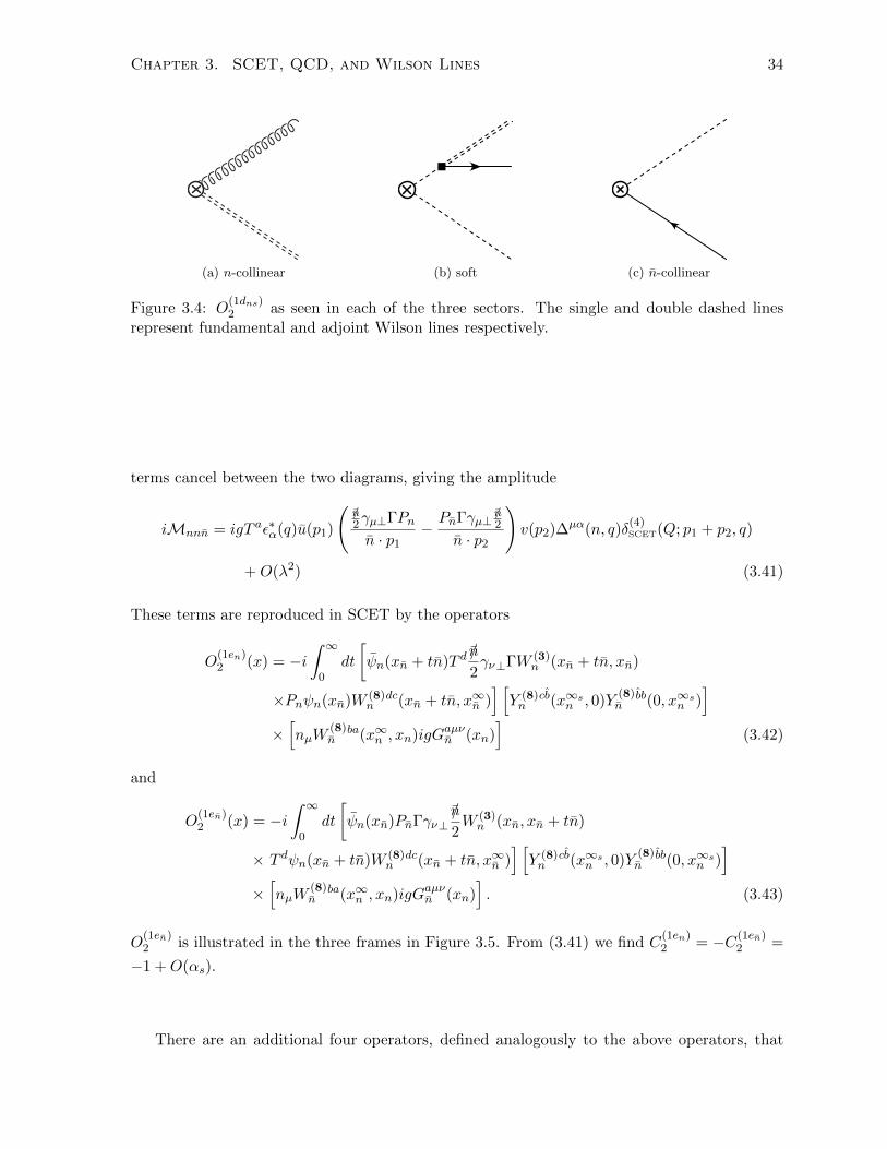
Chapter 3. SCET, QCD, and Wilson Lines 34
(a) n-collinear (b) soft (c) n-collinear
Figure 3.4: O(1dns)2 as seen in each of the three sectors. The single and double dashed lines
represent fundamental and adjoint Wilson lines respectively.
terms cancel between the two diagrams, giving the amplitude
iMnnn = igT aε∗α(q)u(p1)
(/n2γµ⊥ΓPn
n · p1−PnΓγµ⊥
/n2
n · p2
)v(p2)∆µα(n, q)δ
(4)SCET(Q; p1 + p2, q)
+O(λ2) (3.41)
These terms are reproduced in SCET by the operators
O(1en)2 (x) = −i
∫ ∞0
dt
[ψn(xn + tn)T d
/n
2γν⊥ΓW (3)
n (xn + tn, xn)
×Pnψn(xn)W (8)n
dc(xn + tn, x∞n )] [Y (8)n
cb(x∞sn , 0)Y
(8)n
bb(0, x∞sn )]
×[nµW
(8)n
ba(x∞n , xn)igGaµνn (xn)]
(3.42)
and
O(1en)2 (x) = −i
∫ ∞0
dt
[ψn(xn)PnΓγν⊥
/n
2W (3)n (xn, xn + tn)
× T dψn(xn + tn)W (8)n
dc(xn + tn, x∞n )] [Y (8)n
cb(x∞sn , 0)Y
(8)n
bb(0, x∞sn )]
×[nµW
(8)n
ba(x∞n , xn)igGaµνn (xn)]. (3.43)
O(1en)2 is illustrated in the three frames in Figure 3.5. From (3.41) we find C
(1en)2 = −C(1en)
2 =
−1 +O(αs).
There are an additional four operators, defined analogously to the above operators, that

Chapter 3. SCET, QCD, and Wilson Lines 35
(a) n-collinear (b) soft (c) n-collinear
Figure 3.5: O(1en)2 as seen in each of the three sectors.
arise due to corresponding corrections to the n sector:
O(1an)2 (x) =
[ψn(xn)
/n
2W (3)n (xn, x
∞n )
] [Y (3)n (x∞s
n , 0)Y(3)n (0, x∞s
n )]
×[W
(3)n (x∞n , xn)i
←−/D⊥(xn)ΓPnψn(xn)
]O
(1bn)2 (x) =
[ψn(xn)PnW
(3)n (xn, x
∞n )] [Y (3)n (x∞s
n , 0)Y(3)n (0, x∞s
n )]
×[W
(3)n (x∞n , xn)Γi /D⊥(xn)
/n
2ψn(xn)
]O
(1cns)2 (x) = −i
∫ ∞0
dt[ψn(xn)PnW
(3)n (xn, x
∞n )]
(3.44)
×[Y (3)n (x∞s
n , 0)Y(3)n (0, tn)iDµ
⊥(tn)Y(3)n (tn, x∞s
n )]
×[W
(3)n (x∞n , xn)iDµ⊥(xn)ΓPnψn(xn)
]O
(1dns)2 (x) = −i
∫ ∞0
dt[ψn(xn)PnW
(3)n (xn, x
∞n )]
×[Y (3)n (x∞s
n , 0)Γγν⊥/n
2T cY
(3)n (0, tn)ψs(tn)Y
(8)n
cb(tn, x∞sn )
]×[W (8)n
ba(x∞n , xn)igGaνµn (xn)nµ
].
These operators have the same matching coefficients as their n sector counterparts. The one-
gluon Feynman rules for the operators O(1i)2 are shown in Figure 3.6. Loop calculations still
require a zero-bin subtraction [22], which serves to fix the double counting in the same way as
the standard SCET.
Thus, we have shown the primary result of this chapter for e+e− → dijet at O(αs): O(λ)
SCET effects can be written as QCD fields coupled to Wilson lines, where each sector is de-
coupled into a separate SU(3) gauge theory. The only expansion is in the current, and the
subleading operators and physical pictures are generalizations of the O(λ0) operator (3.17) and
physical picture Figure 3.3.

Chapter 3. SCET, QCD, and Wilson Lines 36
p1
p2
p1
p2
p1
p2
(1an)
p1
p2
p1
p2
(1an)
p1
p2
p1
p2
p1
p2
p1
p2
p1
p2
p1
p2
p1
p2
p1
p2 p1
p2
Figure 3.6: One-gluon Feynman rules for NLO dijet operators O(1i)2 . The notation is the same
as Figure 3.2. The rule for O(1bn)2 has been split into two diagrams, depending on whether the
gluon is emitted from the vertex or the Wilson line.
3.4 Heavy-to-Light Current
A similar analysis may be carried out for B → Xsγ decay in the shape function region,
1− y ∼ ΛQCD/mb ∼ λ2 (3.45)
where y = 2Eγ/mb is the scaled energy of the photon. In this region the light final-state hadrons
are constrained to form a jet, and SCET is the appropriate EFT. The SCET analysis of this
process has been carried out to O(λ2) [23,25,32,39]. In this section we present the operators up
to O(λ) in order to show how the picture introduced in this chapter matches the standard SCET
results. The arguments are analogous to the dijet analysis. However, now there is only one
collinear sector and one soft sector, and a copy of the Heavy Quark Effective Theory (HQET)
Lagrangian is necessary. Again, the collinear and soft Lagrangian is not expanded in λ and
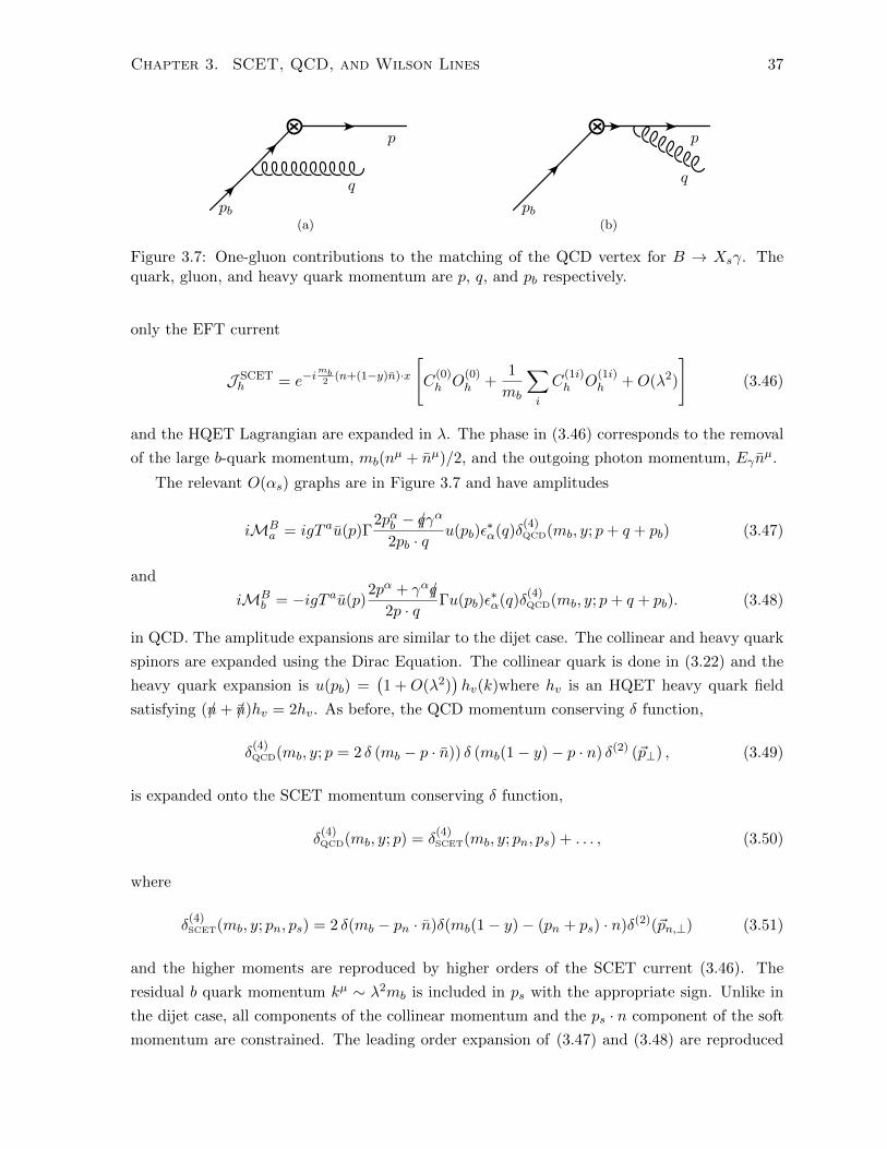
Chapter 3. SCET, QCD, and Wilson Lines 37
pb
p
q
(a)
pb
p
q
(b)
Figure 3.7: One-gluon contributions to the matching of the QCD vertex for B → Xsγ. Thequark, gluon, and heavy quark momentum are p, q, and pb respectively.
only the EFT current
J SCETh = e−i
mb2
(n+(1−y)n)·x
[C
(0)h O
(0)h +
1
mb
∑i
C(1i)h O
(1i)h +O(λ2)
](3.46)
and the HQET Lagrangian are expanded in λ. The phase in (3.46) corresponds to the removal
of the large b-quark momentum, mb(nµ + nµ)/2, and the outgoing photon momentum, Eγn
µ.
The relevant O(αs) graphs are in Figure 3.7 and have amplitudes
iMBa = igT au(p)Γ
2pαb − /qγα
2pb · qu(pb)ε
∗α(q)δ
(4)QCD(mb, y; p+ q + pb) (3.47)
and
iMBb = −igT au(p)
2pα + γα/q
2p · qΓu(pb)ε
∗α(q)δ
(4)QCD(mb, y; p+ q + pb). (3.48)
in QCD. The amplitude expansions are similar to the dijet case. The collinear and heavy quark
spinors are expanded using the Dirac Equation. The collinear quark is done in (3.22) and the
heavy quark expansion is u(pb) =(1 +O(λ2)
)hv(k)where hv is an HQET heavy quark field
satisfying (/n+ /n)hv = 2hv. As before, the QCD momentum conserving δ function,
δ(4)QCD(mb, y; p = 2 δ (mb − p · n)) δ (mb(1− y)− p · n) δ(2) (~p⊥) , (3.49)
is expanded onto the SCET momentum conserving δ function,
δ(4)QCD(mb, y; p) = δ
(4)SCET(mb, y; pn, ps) + . . . , (3.50)
where
δ(4)SCET(mb, y; pn, ps) = 2 δ(mb − pn · n)δ(mb(1− y)− (pn + ps) · n)δ(2)(~pn,⊥) (3.51)
and the higher moments are reproduced by higher orders of the SCET current (3.46). The
residual b quark momentum kµ ∼ λ2mb is included in ps with the appropriate sign. Unlike in
the dijet case, all components of the collinear momentum and the ps · n component of the soft
momentum are constrained. The leading order expansion of (3.47) and (3.48) are reproduced

Chapter 3. SCET, QCD, and Wilson Lines 38
by the operator
O(0)h (x) =
[ψn(x)PnΓW (3)
n (x, x∞c )] [Y (3)n (x∞s
n , xs)hv(xs)]
(3.52)
with C(0)h = 1 +O(αs), which is similar to the leading order label SCET operator [16]
J (0)h = e−i
mb2
(n+(1−y)n)·x ξ(0)n,p(x)W (3)
n (x,∞)ΓY (3)n (∞, x)hv(x). (3.53)
The difference between (3.52) and (3.53) are the use of four-component spinors for the collinear
fields and the fields are at the positions
x = (x · n, x · n, x⊥) xs = (0, x · n, 0)
x∞c = (−∞, x · n, x⊥) x∞sn = (0,∞, 0). (3.54)
The positions are chosen to reproduce (3.51).
The O(λ) expansion of the amplitudes is done in the same way as in the previous section,
so we omit the details. We find the following subleading operators:
O(1ac)h (x) =
[ψn(x)PnΓi /D⊥(x)
/n
2W (3)n (x, x∞c )
] [Y (3)n (x∞s
n , xs)hv(xs)]
O(1bc)h (x) =
[ψn(x)
/n
2i←−/D⊥(x)ΓW (3)
n (x, x∞c )
] [Y (3)n (x∞s
n , xs)hv(xs)]
O(1cs)h (x) = −i
∫ 0
−∞dt[ψn(x)Pni
←−D⊥µ(x)ΓW (3)
n (x, x∞c )]
(3.55)
×[Y (3)n (x∞s
n , xs + tn)i←−Dµ⊥(xs + tn)Y (3)
n (xs + tn, xs)hv(xs)]
O(1ds)h (x) = −i
∫ 0
−∞dt[nµigG
aµνn (x)W (8)
nab(x, x∞c )
]×[Y (8)n
bc(x∞sn , xs + tn)ψs(xs + tn)T c
/n
2γν⊥ΓY (3)
n (xs + tn, xs)hv(xs)
]O
(1δs)h (x) = mb
[ψn(x)PnΓW (3)
n (x, x∞c )] [Y (3)n (x∞s
n , xs)(←−Dµ⊥x⊥µ + x⊥µ
−→D⊥
)(xs)hv(xs)
].
These operators are the analogous dijet operators with only one collinear sector. The opera-
tors O(1cs,1s)h have integration limits −∞ and 0 since the b-quark is coming in from −∞ (as
opposed to the dijet case where the partons are outgoing to +∞). The matching coefficients
are C(1ac,1bc,1δs)h = 1 +O(αs), C
(1ds)h = −1 +O(αs) and C
(1cs)h = 2 +O(αs).
The formulation of SCET introduced in this chapter must be equivalent to standard SCET
formulations at subleading orders. For example, the soft quark operator O(1ds)h is reproduced
by the time-ordered product of L(1)ξq in (3.4) and the leading order current J (0)
h of (3.9), whose
Feynman rules are shown in [32]. A particularly simple example of a subleading standard SCET

Chapter 3. SCET, QCD, and Wilson Lines 39
operator that can be re-written as one of our operators is the O(λ2) label SCET current [21,24]
J (2A) = ξ(x)1
in ·D[in ·D(x)Wc(x, x
∞c )]hv(xs) + . . . , (3.56)
which is identical to the operator we find at O(λ2)
O(2ac)h = −imb
∫ 0
−∞dt[ψn(x)PnW
(3)n (x, x+ tn)in ·D(x+ tn)ΓW (3)
n (x+ tn, x∞c )]
×[Y (3)n (x∞s
n , xs)hv(xs)]
(3.57)
with C(2ac)h = 1 + O(αs). The “. . .” in (3.56) refer to other O(λ2) terms. The equivalence
between (3.56) and (3.57) can be shown using the relations [18,21]
1
in ·DW (3)n (x, x∞c ) = W (3)
n (x, x∞c )1
in · ∂(3.58)
and1
in · ∂φ(x) = −i
∫ 0
−∞dt φ(x+ tn), (3.59)
and the field redefinition (3.5). The relations (3.58) and (3.59) can be used to re-write (3.56)
as
J (2A) = ξ(x)Wc(x, x∞c )
1
in · ∂Wc(x
∞c , x) [in ·D(x)Wc(x, x
∞c )]hv(xs)
= −i∫ 0
−∞dt ξ(0)(x)W (0)
c (x, x+ tn)[in ·D(0)(x+ tn)W (0)
c (x+ tn, x∞c )]
× Yn(x∞sn , xs)hv(xs) (3.60)
= O(2ac)h
where the field redefinition (3.5) and ξ(x) = Pnψ(x) were used in the second line. The other
operators in [21,24] can be shown to be equivalent using the same trick.
3.5 Conclusions
We have demonstrated how SCET can be written as a theory of separate, decoupled sectors
of QCD by explicitly performing the matching of the external current at tree level in αs to
subleading order in λ for both dijet production and B → Xsγ. Interactions between different
sectors are reproduced in SCET by Wilson lines. We believe this makes the SCET picture
more transparent: instead of a complicated collinear Lagrangian that couples two-component
collinear quarks to soft fields, the Lagrangian is just multiple QCD copies. The only expansion
in λ occurs in the currents, which are QCD fields coupled to Wilson lines that represent the
colour flow of the other sectors. The subleading currents are generalizations of the leading order

Chapter 3. SCET, QCD, and Wilson Lines 40
currents akin to higher twist corrections to light-cone distribution functions. Corrections to
leading-order factorization theorems should be simpler since the manifest decoupling of sectors
that occurred at leading order now exists to all orders.

Chapter 4
Subleading Corrections To Thrust
Using Effective Field Theory
In this chapter we calculate the subleading corrections to the thrust rate. We use SCET to
factorize the rate and match onto jet and soft operators that describe the degrees of freedom of
the relevant scales. We work in the perturbative regime where all the scales are well above ΛQCD.
The thrust rate involves an incomplete sum over final states that is enforced by a measurement
operator. Subleading corrections require matching onto not only the higher dimensional dijet
operators, but also matching onto subleading measurement operators in the effective theory.
We explicitly show how to factorize the O(αsτ) thrust rate into a hard function multiplied by
the convolution of the vacuum expectation value of jet and soft operators. Our approach can
be generalized to other jet shapes and rates. The text in this chapter is reproduced in [40].
4.1 Introduction
Jet shapes are examples of observables with multiple scales, which can give rise to logarithmic
enhancements in the fixed order rate that ruin the perturbative expansion in the strong coupling
constant. Effective Field Theories (EFTs) separate the scales by expanding in their small
ratio and matching onto operators that describe the degrees of freedom at each scale. The
logarithmic enhancements are then summed by using the renormalization group to run between
the scales restoring perturbative control of the rate. The effects of the subleading corrections
from the small ratio of scales are systematically calculated in the EFT by matching onto higher
dimensional operators.
The appropriate theory for describing jet shapes with narrow jets is SCET [16–21, 26].
Deriving factorization theorems that separate the scales is straightforward at leading order
(LO) in SCET due to the explicit decoupling of the collinear and soft degrees of freedom.
Subleading corrections to SCET have previously been used to study subleading corrections to
B decays [23]; however, jet shapes are complicated by kinematic cuts placed on the phase space.
41

Chapter 4. Subleading Corrections To Thrust Using EFT 42
The goal of this chapter is to demonstrate how to factorize the subleading corrections to jet
shapes using SCET by considering the example of the thrust observable.
Thrust [9] is defined by
τ =1
Q
∑i∈X
min(Ei + ~t · ~pi, Ei − ~t · ~pi
), (4.1)
where Q is the initial energy, X is the final state, and the thrust axis ~t is the unit vector that
maximizes∑
i∈X |~t · ~pi|. When τ � 1 the final state is a pair of back-to-back jets with small
invariant mass. Thrust is a convenient observable to illustrate how to calculate subleading jet
shapes in SCET due to its simple phase space. We will concern ourselves only with e+e− →γ∗ → X in order to reduce the contribution from initial state radiation and restrict ourselves
to vector currents. It is possible to generalize to weak process but for simplicity, we will not
consider axial currents in this chapter.
The LO in τ thrust rate was calculated using SCET in [41,42]. The rate was written in the
factorized form
H × 〈0|J |0〉 ⊗ 〈0|J |0〉 ⊗ 〈0|S|0〉+O(τ), (4.2)
where the convolution is defined in Section 4.3. The LO rate was factorized by matching
onto SCET and expanding the final state phase space imposed by (4.1) in the SCET power
counting. The jet operators, J and J , describe the physics at the intermediate scale√τQ, the
soft operator, S, describes the physics at the soft scale τQ, and the hard function, H, describes
the physics above the hard scale Q. Factorization allows the large ln τ ’s to be summed by
separately renormalizing the jet and soft operators. This was done in [42].
We are interested in extending the results of [41, 42] to include the O(τ) corrections to the
rate. We restrict our calculation to the perturbative regime when the soft scale is well above
ΛQCD. We will ignore the effects of hadron masses, which have been discussed in [43]. We
will show how the O(τ) rate can be factorized as in (4.2) using SCET with the appropriate
subleading jet and soft operators. These subleading operators are generalizations of the LO
operators, and properly separate the scales while having consistent power counting. We leave
renormalizing these operators to a future work.
Understanding how to incorporate subleading phase space effects is important for writing
a factorization theorem beyond LO. We will show how subleading phase space is accounted for
in the effective theory by 1) consistent expansion of the cuts using the SCET power counting,
and 2) insertions of subleading operators that account for the QCD momentum conservation
expansion. Both these effects must be accounted for in order to calculate the O(τ) corrections
to the rate and reproduce the perturbative QCD result at O(αsτ) in [44].
The rest of the chapter is organized as follows: in Section 4.2 we review the description
of SCET in [26] and explain our reasoning for using this formulation over the formulation
in [16–20]. In Section 4.3 we review the LO calculation and introduce the notation used in the
rest of the chapter. We calculate the O(αsτ) rate in Section 4.4 and demonstrate how to write

Chapter 4. Subleading Corrections To Thrust Using EFT 43
it in a factorized form. We conclude in Section 4.5. The full list of operators is reserved for the
appendices.
For simplicity we use the notation LH ≡ ln(µ2/Q2), LJ ≡ ln(µ2/(Q√τ)2), LS ≡ ln(µ2/(Qτ)2),
and αs ≡ αsCF /(2π) where CF = (N2C − 1)/(2NC) for NC colours.
4.2 Review of SCET
Soft-Collinear Effective Theory describes the interactions between highly boosted and low en-
ergy degrees of freedom. Three types of fields are required for calculating thrust: n-collinear,
n-collinear, and soft, which have characteristic momentum scaling∗ in terms of the SCET ex-
pansion parameter λ� 1
pµn ∼ Q(λ2, 1, λ), pµn ∼ Q(1, λ2, λ), kµs ∼ Qλ2 (4.3)
respectively. The two collinear sectors describe fields that are highly energetic and moving in
opposite directions, while the soft sector describes low energy fields. The SCET Lagrangian and
operators are derived by expanding the interactions between the different fields in λ. Momenta
denoted by k will be O(λ2)Q unless otherwise specified.
We will use the SCET formulation of [26]. In this formulation, soft and collinear fields are
described by QCD in the absence of an external current. Therefore, the SCET Lagrangian is
LSCET = LnQCD + LnQCD + LsQCD, (4.4)
which has no subleading contributions and each LmQCD will describe fields from the m sector
only. The interactions between the sectors are contained in the external currents. The QCD
vector current
J2µ(x) = ψ(x)γµψ(x) (4.5)
is matched onto the SCET dijet operators
J2µ → C
(0)2 O
(0)µ2 +
1
Q
∑i≥1
C(i)2 O
(i)µ2 + . . . (4.6)
where the superscripts denote the suppression in λ and the ellipses represent higher dimensional
operators. The operators and their tree-level matching coefficients C(i)2 are found by expanding
the diagrams in Figure 4.1 in λ for n-collinear, n-collinear, and soft fields.
At LO, the (anti-)quark must be (n-)n-collinear and the gluon can be either collinear or
∗The momentum pµ = (p+, p−, p⊥) is defined in light-cone coordinates by p+ ≡ p ·n = E− ~p · ~n, p− ≡ p · n =E + ~p · ~n, and pµ⊥ = pµ − p+ nµ
2− p− n
µ
2where n · n = 2.

Chapter 4. Subleading Corrections To Thrust Using EFT 44
(a) (b)
Figure 4.1: QCD vertex diagrams required for dijet production at O(αs).
soft. The LO dijet operator is [26]
O(0)µ2 (x) =
[ψn(xn)PnW
(3)n (xn, x
∞n )] [Y (3)n (x∞s
n , 0)γµY(3)n (0, x∞s
n )] [W
(3)n (x∞n , xn)Pnψn(xn)
],
(4.7)
with one-loop matching coefficient [45]
C(0)2 (µ) = 1− αs
(1
2ln2
(µ2
−Q2
)+
3
2ln
(µ2
−Q2
)+ 4− π2
12
)+O(α2
s) (4.8)
and MS counterterm
Z(0)2 (µ) = 1 + αs
(− 1
ε2− 3
2ε− 1
εln
(µ2
−Q2
))+O(α2
s). (4.9)
The interactions between the different sectors are reproduced by Wilson lines defined in a
representation R
W (R)n (x, y) = P exp
(−ig
∫ n2·(y−x)
0ds n ·Aan(x+ ns)T aR
)
Y (R)n (x, y) = P exp
(−ig
∫ n2·(y−x)
0ds n ·Aas(x+ ns)T aR
)(4.10)
with similar definitions for W(R)n and Y
(R)n . The projectors Pn = (/n/n)/4 and Pn = (/n/n)/4 are
required from the expansion of the Dirac equation. The positions are defined as
xn = (0, x · n, ~x⊥) x∞n = (0,∞, ~x⊥) x∞sn = (0,∞, 0)
xn = (x · n, 0, ~x⊥) x∞n = (∞, 0, ~x⊥) x∞sn = (∞, 0, 0) (4.11)
and are necessary to conserve the appropriate components of momentum that respect (4.3).
Each square bracket in (4.7) is a separately gauge invariant piece, which means the sectors
explicitly decouple from one another. The physical interpretation of the operator is given
in [26].

Chapter 4. Subleading Corrections To Thrust Using EFT 45
The next-to-leading order (NLO) dijet operators and matching coefficients were found in [26]
and are reproduced in Section 4.6. The operators are generalizations of the LO operator (4.7)
with appropriate derivative insertions. For O(τ) corrections to thrust, we will also need the
N2LO operators, which are found by following the approach of [26]. These operators and their
matching coefficients are also shown in Section 4.6. Both the NLO and N2LO dijet operators
explicitly decouple the sectors in the same way as the LO operator.
A more widely used formulation of SCET [16–20] separates the collinear momentum into
p = p+k, where k ∼ λ2Q and p ∼ Q,λQ are the residual and label momentum respectively. The
large label momentum is removed from all interactions leading to the Lagrangian being a non-
local expansion of two-component spinors with soft and collinear fields explicitly interacting at
NLO. Although, the formalisms of [16–20] and [26] are equivalent, they approach momentum
conservation differently. This is important when cuts are placed on phase space such as for
the thrust rate. In the approach of [26], momentum is not conserved and the subleading
O(δ)2 operators in Section 4.6 account for the expansion of QCD momentum conservation using
SCET momentum power counting. In the approach of [16–20], label and residual momentum
are separately conserved meaning momentum is exactly conserved. The equivalent action of
the O(1δ)2 operator comes from the subleading kinetic interaction [46]
L(1)ξξ
∣∣gs=0
=∑p,p′
ξn,p(x)i/∂⊥1
P/P⊥ /n
2ξn,p′(x) + h.c (4.12)
where ξn,p is a two-component n-collinear spinor with label momentum p, and Pµ is an oper-
ator that pulls down label momentum. Insertions of this term into time-ordered products is
equivalent to expanding the on-shell condition (p+k)2 = 0 in λ. These terms are not necessary
for inclusive phase space calculations such as subleading B decays [23]. However, they will
be important when cuts are placed on phase space such as in the subleading thrust rate and
reproduce the action of the O(1δ)2 operator in time-ordered products.
In this chapter we choose to use the formalism of [26]. The Lagrangian of [26] has simpler
Feynman rules and only one insertion of O(1δ)2 is required instead of an insertion of L(1)
ξξ for each
collinear field. The explicit decoupling of sectors at the operator level also makes it easier to
derive a subleading factorization theorem.
4.3 Leading Order Calculation
The LO thrust distribution was calculated using the approach of [16–20] in [42] and was written
in the factorized form (4.2). In this section we review the calculation using the formalism of [26],
which gives an equivalent form of the answer. In the next section we generalize this description
to calculate the O(τ) rate.

Chapter 4. Subleading Corrections To Thrust Using EFT 46
The thrust rate is the cumulate of the distribution
R(τ) =1
σ0
∫dτ ′
dσ
dτ ′θ(τ − τ ′) =
∫d4xe−iQ·x〈0|J2
µ†(x)MQCD(τ)J2µ(0)|0〉 (4.13)
where Qµ = (Q/2)(nµ + nµ) is the momentum of the incoming photon and σ0 is the Born
cross-section. The measurement operator, MQCD(τ) [41,47], acts on states |X〉
MQCD(τ)|X〉 ≡ MQCD(τ, {pX})|X〉 (4.14)
to project only those final states that give a thrust value τ . When taking the cuts of diagrams,
the functionMQCD(τ, {pX}) generates the appropriate phase space by restricting the momentum
of the particles {pX}.
To factorize the rate, we first match the QCD currents and measurement operators onto
SCET dijet and measurement operators. The matching of the QCD currents onto SCET dijet
operators was discussed in Section 4.2. The QCD measurement operators are matched onto
SCET measurement operators in a similar manner
MQCD(τ)→ M(0)(τ) + M(1)(τ) + M(2)(τ) +O(λ3),
where the superscripts refer to the suppression in λ. The SCET measurement operators are
found by expanding the thrust constraints implemented byMQCD using the SCET momentum
scaling (4.3).
Thrust is measured with respect to the thrust axis, ~t, defined below (4.1). The definition of
the thrust axis in SCET has an expansion in λ and is written as ~t = ~t (0) + O(λ2). The SCET
momentum power counting defines the LO thrust axis ~t (0) = −~n [41], where we have chosen the
−~n axis to be exactly along the total n-collinear momentum (i.e. ~pn⊥ ≡ 0). The overall sign of
~t is unimportant as seen in (4.1). The sectors decouple in the LO measurement operator [41,42]
M(0)(τ) = M(0)n (τn)⊗ M(0)
n (τn)⊗ M(0)s (τs) (4.15)
because the thrust axis is independent of any individual particle. The convolution above is
defined as
f1(τ1)⊗ f2(τ2)⊗ f3(τ3) ≡∫dτ1dτ2dτ3θ(τ − τ1 − τ2 − τ3)f1(τ1)f2(τ2)f3(τ3). (4.16)

Chapter 4. Subleading Corrections To Thrust Using EFT 47
Using the LO definition of the thrust axis, the action of the measurement operators are
M(0)n (τ, {p}) =
(∑i p−i
Q
)d−2
δ
(τ − 1
Q
∑i
|~pi⊥|2
p−i
)
M(0)n (τ, {p}) =
(∑i p
+i
Q
)d−2
δ
(τ − 1
Q
∑i
|~pi⊥|2
p+i
)
M(0)s (τ, {k}) = δ
(τ − 1
Q
(n · k(0)
+t + n · k(0)−t
))(4.17)
where the sums are only over the momentum in each sector. We have defined
kµ±t =∑i
kµi θ(±~ki · ~t ) = k(0)µ±t + k
(2)µ±t +O(λ4) (4.18)
as the total soft momentum in the ±~t hemisphere. The LO definition is
k(0)µ±t =
∑i
kµi θ(±~ki · ~t(0)) =
∑i
kµi θ(∓~ki · ~n), (4.19)
where in both (4.18) and (4.19) the sum is over all soft particles. The d = 4 − 2ε dependent
prefactors in the collinear sectors come from choosing the collinear fields to be in the nµ and nµ
directions. At LO these prefactor have no affect, but are important for the O(τ) corrections.
By matching the QCD operators in (4.13) onto the SCET operators, the LO thrust rate is
written as
R(τ) = |C(0)2 |
2
∫ddxe−iQ·x〈0|O(0)µ†
2 (x)M(0)(τ)O(0)2 µ(0)|0〉+O(τ) (4.20)
where the O(τ) corrections will be calculated by the subleading in λ operators. The rate is
factorized by matching above the operator product onto jet and soft operators∫ddx e−iQ·xO
(0)µ†2 (x)M(0)(τ)O
(0)2µ (0) = C(0)J (0)(τn)⊗ J (0)(τn)⊗ S(0)(τs) (4.21)
with matching coefficient C(0). As usual, the superscripts on the jet and soft operators refer to
their suppression in λ. The rate can then be written in the desired factorized form
R(τ) = H(0)(µ)〈0|J (0)(µ, τn)|0〉 ⊗ 〈0|J (0)(µ, τn)|0〉 ⊗ 〈0|S(0)(µ, τs)|0〉+O(τ) (4.22)
where the hard function
H(0)(µ) = |C(0)2 (µ)|2C(0)(µ) (4.23)
is the product of the matching coefficients.
The explicit decoupling of n-collinear, n-collinear, and soft degrees of freedom in the dijet

Chapter 4. Subleading Corrections To Thrust Using EFT 48
0 xn
(a) 〈0|J(0)|0〉 (b) 〈0|J(0)|0〉 (c) 〈0|J(0)|0〉 (d) 〈0|J(0)|0〉
n n
nn
(e) 〈0|S(0)|0〉 (f) 〈0|S(0)|0〉 (g) 〈0|S(0)|0〉 (h) 〈0|S(0)|0〉
Figure 4.2: One-loop diagrams of (4.25). Solid lines represent fermions, dashed lines representWilson lines with the colour flowing in the direction of the arrows, and the dots representLagrangian insertions. The type of soft Wilson lines are labelled in Figure 4.2e. The cut isdistinguished by the bold vertical dashed line. The contributions to J (0) look identical to thecontributions of J (0) after a rotation of 180◦.
and measurement operators makes finding the appropriate jet and soft operators straightfor-
ward. Using the Fierz identity to separate the spin and colour indices, we find the operators
are
J (0)(µ, τ) =1
NCTr
∫dx+dd−2x⊥e
−iQx+ψn(0)W (3)
n (0, x∞sn )
/n
2M(0)
n (τ)W (3)n (x∞n , xn)ψn(xn)
J (0)(µ, τ) =1
NCTr
∫dx−dd−2x⊥e
−iQx−ψn(xn)W(3)n (xn, x
∞n )
/n
2M(0)
n (τ)W(3)n (x∞s
n , 0)ψn(0)
S(0)(µ, τ) =1
NCTrY
(3)n (x∞s
n , 0)Y (3)n (0, x∞s
n )M(0)s (τ)Y (3)
n (x∞sn , 0)Y
(3)n (0, x∞s
n ), (4.24)
where the trace is over spins and colour. These operators give the same Feynman rules as
those found in [42]. The matching coefficient in (4.21) is most easily found by comparing
the vacuum expectation value of both sides. The real emission contributions to the one-loop
vacuum expectation value of J (0) and S(0) are pictured in Figure 4.2. They are calculated by
cutting the diagrams along the vertical dashed lines and applying the measurement operator
to the fields passing through this cut [42]. The virtual diagrams are scaleless and thus zero in

Chapter 4. Subleading Corrections To Thrust Using EFT 49
MS. The vacuum expectation value of the jet and soft operators are [42]
〈0|J (0)(µ, τ)|0〉 = δ(τ)
[1 + αs
(2
ε2+
2
εLH +
3
2ε+ L2
H +3
2LH +
7
2− π2
2
)]+ αs
[(− 2
ε− 3
2− 2LJ
)(θ(τ)
τ
)]+
〈0|J (0)(µ, τ)|0〉 = 〈0|J (0)(µ, τ)|0〉 (4.25)
〈0|S(0)(µ, τ)|0〉 = δ(τ)
[1 + αs
(− 2
ε2− 2
εLH − L2
H +π2
6
)]+ αs
[(4
ε+ 4LS
)(θ(τ)
τ
)]+
,
where we have included the zero-bin procedure [22], which accounts for the double counting
between the collinear and soft operators. The matching coefficient C(0)(µ) = 1 [42] meaning
the hard function is
H(0)(µ) = 1 + αs
(L2H − 3LH − 8 +
7π2
6
)+O(α2
s). (4.26)
As expected, the jet and soft operators separate the√τQ and τQ scales. The hard function
describes the physics above the cut-off Q, of the effective theory.
Matrix elements of the jet and soft operators also do not need any further expansion in
τ . This is required to ensure that operators of different orders do not mix. We note that this
is different than the results in [35], which considered the exclusive JADE two-jet rate at LO.
This rate has the same O(αs) phase space as the thrust rate in QCD. In [35], the phase space
was not consistently expanded in λ and an expansion in τ was required after the phase space
integration. A subleading zero-bin procedure is necessary to ensure that the LO operators do
not contribute to subleading corrections. In this chapter and in [42], the measurement operator
is consistently expanded in λ so matrix elements of the jet and soft operators automatically
have consistent power counting.
The thrust rate at O(αsτ0) is calculated by substituting the hard function and the vacuum
expectation values of the jet and soft operators into (4.22). The rate is found to be
R(τ) = 1 + αs
(−2 ln2 τ − 3 ln τ +
π2
3− 1
)+O(α2
s, τ),
which reproduces the rate found in perturbative QCD at this order [42]. By separately renor-
malizing the jet and soft operators the large ln τ ’s were summed in [42]. In the next section we
follow the same procedure to find the O(αsτ) correction to the rate and write it in a factorized
form analogous to (4.22).

Chapter 4. Subleading Corrections To Thrust Using EFT 50
4.4 Next-to-Leading Order Calculation
The results are extended to include the O(τ) corrections by systematically matching the QCD
current and measurement operator in (4.13) onto subleading SCET dijet and measurement
operators. The O(τ) thrust rate in SCET is written as
R(τ) =∑
i+j+k≤2
C(i)∗2 C
(j)2
∫d4xe−iQ·x〈0|O(i)†µ
2 (x)M(k)(τ)O(j)2µ (0)|0〉+O(τ2). (4.27)
From the LO calculation λ ∼√τ , so we need the O(λ2) SCET operators as illustrated by the
constraints on the sum. One can explicitly check that the O(λ) corrections, which would give
O(√τ) corrections, vanish.
As in the previous section, we want to write (4.27) in a factorized form by matching onto
subleading jet and soft operators. These operators will be generalizations of the LO operators
and their matrix elements must have a consistent power counting in τ as in the LO case. We
will only do the tree-level matching, which is all that is necessary to calculate the O(αsτ)
rate. The subleading dijet operators are written in Section 4.6 and explicitly decouple the
sectors. We must also find the subleading measurement operators, M(1,2)(τ) in (4.15). We
will show in the next section that the action of the subleading measurement operators also
decouples the sectors, analogously to (4.15). The explicit decoupling of the sectors in the dijet
and measurement operators makes writing the rate in the desired factorized form in Section
4.4.2 straightforward.
4.4.1 Measurement Operator
The action of the subleading measurement operators are found by first expanding the definition
of the thrust axis and then finding this expansion’s effect on the measurement of thrust. The
thrust axis is defined as the unit vector that maximizes the sum below (4.1). The sum is
maximized when the thrust axis is in the direction of the hemisphere with the largest three-
momentum, ~p+t [41]. Therefore, the thrust axis is written in SCET as the expansion
~t =~p+t
|~p+t|= ~t (0) + ~t (2) + ~t (4) +O(λ6), (4.28)
where the superscripts refer to the suppression in λ.
In order to find ~p+t, we first note that the n-collinear and n-collinear particles are always in
opposite hemispheres. SCET momentum power counting enforces this at LO and the zero-bin
procedure will enforce this at all orders in λ. Therefore, the total momentum of the hemisphere
will be
~p+t = ~pn + ~k+t, (4.29)
where pµn is the total n-collinear momentum and kµ+t is the total soft momentum in the +~t
hemisphere as defined in (4.18). The expansion of (4.18) and (4.28) allows us to iteratively

Chapter 4. Subleading Corrections To Thrust Using EFT 51
solve for both ~t (i) and k(i)µ±t . The subleading corrections to the thrust axes are
~t (2) =2~k
(0)+t⊥p+n
(4.30)
~t (4) =2(~k
(0)+t⊥)2
(p+n )2
~n+(2~n · ~k(0)
+t + k−n )
(p+n )2
~k(0)+t⊥ +
2~k(2)+t⊥p+n
where k−n is the total n-collinear momentum in the nµ direction. The subleading correction to
the total soft momentum in each hemisphere
k(2)µ+t = −k(2)µ
−t =1
p+n
∑i
kµi
(2~k
(0)+t⊥ · ~ki⊥
)δ(−~n · ~ki) (4.31)
is found by inserting the ~t (2) into (4.18). The first equality above is because the sum of the soft
momentum in the two hemispheres must be O(λ2).
We note we could have instead used −~p+t = ~pn + ~k−t in (4.28), where ~pn is the total n-
collinear momentum and ~k−t is the total soft momentum in the −~t hemisphere. However, the
definition in (4.29) is simpler due to our choice of ~n in Section 4.3 such that ~pn⊥ = ~0. The
apparent asymmetry in the labelling of nµ and nµ in the resulting phase space will be accounted
for by the O(1δ)2 and O
(2δ⊥)2 operators in Section 4.6. The choice of ~pn⊥ ≡ ~0 means the Feynman
rules of these operators involve ∂/∂~pn⊥’s only.
The subleading measurement operators are found by substituting the corrections to the
thrust axis into (4.1). We first consider the contribution from an n-collinear particle with
momentum pi. As discussed in the second paragraph of this section, Ei + ~pi · ~t is always the
minimum for each n-collinear particle. Therefore, the n-collinear sector contributes
1
Q
∑i
(Ei + ~pi · ~t (0)) +1
Q
(~t (2) + ~t (4)
)·∑i
~pi +O(λ5) (4.32)
to the thrust, where the sum is only over n-collinear particles. The first term reproduces the
action of the LO measurement operator in (4.17). The t(2) term gives the NLO correction
and the first term of t(4) in (4.30) gives the N2LO correction. This power counting is due to
p⊥i ∼ O(λ)Q for n-collinear particles.
The contribution to thrust from the n-collinear particles is found in a similar way. Here,
the Ei − ~pi · ~t is always the minimum so the n-collinear sector contributes
1
Q
∑i
(Ei − ~pi · ~t (0))− 1
Q~t (4) ·
∑i
~pi +O(λ5), (4.33)
where the sum is only over n-collinear particles. The first term is the LO contribution and the
second term is the N2LO contribution. There is no ~t (2) term because we have set ~pn⊥ = ~0 by
our choice of ~n.

Chapter 4. Subleading Corrections To Thrust Using EFT 52
Unlike the collinear particles, soft particles can be in either hemisphere. The minimum of
Ei ± ~t · ~ki is determined by which hemisphere the soft particle is in. Therefore, the soft sector
contributes
1
Q
(n · k(0)
+t + n · k(0)−t
)+
1
Q
(n · k(2)
+t + n · k(2)−t + ~t (2) ·
(~k
(0)+t − ~k
(0)−t
))+O(λ6). (4.34)
to the total thrust. The first line is the LO contribution in (4.17) and the remaining terms are
all N2LO.
The action of the subleading measurement operators is found by Taylor expanding the
contribution to thrust in λ. We incorporate the NLO and N2LO corrections from the collinear
sectors in (4.32) and (4.33) by writing the action of the subleading measurement operators as
M(1n)(τ, {pn, pn, ks}) =
(pαn⊥Q
∂
∂τnM(0)
n (τn, {pn}))⊗(Q
p+n
M(0)n (τn, {pn})
)⊗
(−2k
(0)α+t⊥Q
M(0)s (τs, {ks})
)
M(2na)(τ, {pn, pn, ks}) =
(pαn⊥p
βn⊥
Q2
∂2
∂τ2n
M(0)n (τn, {pn})
)⊗(Q2
p+2n
M(0)n (τn, {pn})
)
⊗
(2k
(0)α+t⊥k
(0)β+t⊥
Q2M(0)
s (τs, {ks})
)
M(2nb)(τ, {pn, pn, ks}) =
(p−nQ
∂
∂τnM(0)
n (τn, {pn}))⊗(
Q2
(p+n )2M(0)
n (τn, {pn}))
⊗
(−(~k
(0)+t⊥)2
Q2M(0)
s (τs, {ks})
)(4.35)
M(2nb)(τ, {pn, pn, ks}) =M(0)n (τn, {pn})⊗
(p+n
Q
∂
∂τnM(0)
n (τn, {pn}))
⊗
((~k
(0)+t⊥)2
Q2M(0)
s (τs, {ks})
).
M(2na) comes from the second term in the expansion of the NLO correction in (4.32). The
N2LO corrections from the soft sector in (4.34) are incorporated by the subleading measurement
operators
M(2si)(τ, {pn, pn, ks}) =M(0)n (τn, {pn})⊗
(Q
p+n
M(0)n (τn, {pn})
)⊗M(2si)
s (τs, {ks}) (4.36)

Chapter 4. Subleading Corrections To Thrust Using EFT 53
where
M(2s1)s (τ, {ks}) =
2~k(0)+t⊥ · ~k
(0)+t⊥
Q
∂
∂τsM(0)
s (τs, {ks})
M(2s2)s (τ, {ks}) =
−2~k(0)+t⊥ · ~k
(0)−t⊥
Q
∂
∂τsM(0)
s (τs, {ks})
M(2s−t)s (τ, {ks}) =
p+nn · k
(2)+t
Q2
∂
∂τsM(0)
s (τs, {ks}) (4.37)
M(2s+t)s (τ, {ks}) =
p+n n · k
(2)−t
Q2
∂
∂τsM(0)
s (τs, {ks}).
The p+n in the action of the soft measurement operators M(2s±t) are introduced to cancel the
p+n in (4.31).
The actions of the measurement operators (4.35) and (4.36) define the NLO and N2LO
measurement operators M (1,2)(τ). As the brackets suggest, the sectors explicitly decouple in
the action of the subleading measurement operators. This is due to the corrections to thrust
depending only on the total momentum of each collinear sector and not any individual particle.
While it is possible to formally write the subleading measurement operators using the energy-
flow operator [41,42] and not just their actions in momentum space, we see no reason to do so:
only their actions in momentum space are necessary in calculations.
We note that the measurement operators in this section are found using the formalism of [26]
and would be different if we used the SCET formalism of [16–20]. It was suggested in [41] the
subleading measurement operators could be found using the subleading terms in the SCET
Lagrangian of [16–20]. While we do not explicitly check this, we note that the breaking of the
explicit decoupling of soft and collinear fields in the subleading Lagrangian would complicate
factorization.
4.4.2 Factorization
The explicit decoupling of the sectors in the subleading dijet and measurement operators makes
it straightforward to factorize the subleading corrections to the rate. In order to factorize the
rate, each operator product in (4.27) is matched onto the appropriate jet and soft operators∫ddxO
(i)†2 (x)M(k)(τ)O
(j)2 (0) =
∑α(l,m,n)
C(i,j,k)α J (l)(τn)⊗ J (m)(τn)⊗ S(n)(τs) (4.38)
+ τ C(i,j,k)0 J (0)(τn)⊗ J (0)(τn)⊗ S(0)(τs),
with matching coefficients C(i,j,k)α,0 . The last line is made N2LO by the explicit τ in front. The
integer α ≥ 1 labels the combination of jet and soft operators and we require i + j + k = 2 =

Chapter 4. Subleading Corrections To Thrust Using EFT 54
l +m+ n. The O(τ) rate can then be written in the factorized form
R(2)(τ) =∑i,j,k,α
H(i,j,k)α (µ)〈0|J (l)(µ, τn)|0〉 ⊗ 〈0|J (m)(µ, τn)|0〉 ⊗ 〈0|S(n)(µ, τs)|0〉
+ τ∑i,j,k
H(i,j,k)0 (µ)〈0|J (0)(µ, τn)|0〉 ⊗ 〈0|J (0)(µ, τn)|0〉 ⊗ 〈0|S(0)(µ, τs)|0〉 (4.39)
where the hard functions are defined as
H(i,j,k)α,0 (µ) = C
(i)∗2 (µ)C
(j)2 (µ)C
(i,j,k)α,0 (µ). (4.40)
This generalizes the LO factorization (4.22) to incorporate the N2LO corrections and is the
main result of our chapter. While it is possible to calculate the O(αsτ) rate directly from
(4.27), the factorized form will allow the jet and soft operators to be renormalized separately.
Below we will use a few examples to demonstrate how the jet and soft operators in (4.38)
are found. The full list of operators and their matching coefficients are found in Section 4.7. For
the sake of brevity, we only write those operators that contribute to the O(αsτ) rate. We omit
the phase space integrals when calculating matrix elements of the operators to avoid potentially
confusing the reader.
A) i = 1an, j = 1bn, k = 0 : The operators are found in (3.34). The left-hand side of
(4.38) is
−∫ddxe−iQ·x
1
Q
[ψn(xn)W
(3)n (xn, x
∞n )] [Y
(3)n (x∞s
n , 0)Y (3)n (0, x∞s
n )]
×[W (3)n (x∞n , xn)i
←−Dβ1
⊥ (xn)Γβ1µ1 ψn(xn)
]M(0)
n (τn)⊗ M(0)n (τn)⊗ M(0)
s (τs) (4.41)
× 1
Q
[ψn(0)i
←−Dβ2
⊥ (0)Γβ2µ2 W (3)
n (0, x∞sn )] [Y (3)n (x∞s
n , 0)Y(3)n (0, x∞s
n )] [W
(3)n (x∞s
n , 0)ψn(0)]
where Γαµ1 = /n2γ
α⊥γ
µPn and Γαµ2 = /n2γ
α⊥γ
µPn and γµ⊥ is defined in Section 4.7. The 1/Q’s come
from the definition of the operator expansion (4.6) and the negative sign comes from taking the
hermitian conjugate. The square brackets denote the separately gauge invariant pieces of each
sector. As for the LO factorization, we use the Fierz identity to separate the spin and colour
indices and match onto the appropriate jet and soft operators
C(1an,1bn,0)1 J (2abn)(τn)⊗ J (0)(τn)⊗ S(0)(τs) + τ C
(1an,1bn,0)0 J (0)(τn)⊗ J (0)(τn)⊗ S(0)(τs). (4.42)
The LO operators J (0), J (0) and S(0) are defined in (4.24) and the subleading jet operator is
J (2abn)(µ, τ) =1
Q2NCTr
∫dx+dd−2x⊥e
−iQx+ψn(0)iDα
⊥(0)W (3)n (0, x∞s
n ) (4.43)
× /n
2M(0)
n (τ)W (3)n (x∞n , xn)iD⊥α(xn)ψn(xn). (4.44)

Chapter 4. Subleading Corrections To Thrust Using EFT 55
(a) (b) (c)
Figure 4.3: Matrix element 〈0|J (2abn)|0〉 that give non-zero τ values at O(αs).
The operator is suppressed by λ2 due to the derivative insertions. The vacuum expectation
value of this operator is shown in Figure 4.3.
In order to find the matching coefficients, we calculate the vacuum expectation value of
(4.41) and (4.42). The Feynman rules for the dijet operators were written in [26], and we find
the vacuum expectation value of (4.41) is
− 1
2αsτ +O(α2
s). (4.45)
The vacuum expectation values of J (0), J (0), and S(0) were found in (4.24) and the diagrams
in Figure 4.3 lead to
〈0|J (2abn)(µ, τ)|0〉 =1
2αs +O(α2
s). (4.46)
Here and in the calculations below we have included the zero-bin procedure. As expected, the
matrix element of the J (2abn) operator is suppressed by τ ∼ λ2 compared to the LO jet operator.
The matching coefficients are found to be C(1an,1bn,0)1 = −1+O(αs) and C
(1an,1bn,0)0 = 0+O(α2
s)
meaning the hard functions are
H(1an,1bn,0)1 (µ) = 1 +O(αs)
H(1an,1bn,0)0 (µ) = 0 +O(α2
s). (4.47)
Therefore, the contribution of (4.41) to the rate can be written in the factorized form (4.39),
with the appropriate subleading jet operator.
B) i = 2δn, j = k = 0 : The operator O(2δn)2 is shown in (4.59) and accounts for the
matching of QCD momentum conservation onto SCET momentum conservation at O(λ2). The
contribution where j = 2δn in (4.38) means taking O(2δn)2 (0), which vanishes due to the explicit
x dependence in the dijet operator. As in the previous example, we use the Fierz identity to
factorize the contribution from this operator and match onto∫ddxO
(2δn)†2 (x)M(0)(τ)O
(0)2 (0) = C
(2δn,0,0)1 J (2δn)(τn)⊗ J (0δn)(τn)⊗ S(0)(τs)
+ τ C(2δn,0,0)0 J (0)(τn)⊗ J (0)(τn)⊗ S(0)(τs), (4.48)

Chapter 4. Subleading Corrections To Thrust Using EFT 56
where the new jet operators are
J (2δn)(τ) =1
QNCTr
∫dx+dd−2x⊥e
−iQx+ψn(0)W (3)
n (0, x∞sn )
× /n
2M(0)
n (τ)W (3)n (x∞n , xn)
(in ·←−D + in ·D
)(xn)ψn(xn) (4.49)
J (0δn)(τ) =iQ
NCTr
∫dx−dd−2x⊥e
−iQx− x−ψn(xn)W(3)n (xn, x
∞n )
× /n
2M(0)
n (τ)W(3)n (x∞s
n , 0)ψn(0).
The derivatives in J (2δn) pull down the O(λ2) component of the n-collinear momentum leading
to a λ2 suppression compared to the LO jet operator. The x− dependence of O(2δn)2 is put
into J (0δn) because only the n-collinear fields depend on this coordinate. We have introduced
the Q’s so the operators will have the correct mass dimensions. The diagrams of the vacuum
expectation value of J (2δn) and J (0δn) are the same as the diagrams of the vacuum expectation
value of J (0) and J (0) in Figure 4.2.
As before, the matching coefficient is most easily determined by comparing the vacuum
expectation value of both sides of (4.48). The explicit x− in both O(2δn)2 and J (0δn), which is
a derivative ∂/∂p+n in momentum space, acts on the d-dependent prefactor in M(0)
n of (4.17).
Therefore, the vacuum expectation value of the left-hand side of (4.48) is
αsτ
(−4
ε− 4LJ − 3
)+O(α2
s). (4.50)
and the vacuum expectation value of the jet operators are
〈0|J (2δn)(µ, τ)|0〉 = αs
(−2
ε− 2LJ −
3
2
)+O(α2
s)
〈0|J (0δn)(µ, τ)|0〉 = 2δ(τ) +O(αs). (4.51)
Comparing both sides of (4.48) we find the matching coefficients are C(2δn,0,0)1 (µ) = 1 +O(αs)
and C(2δn,0,0)0 (µ) = αs +O(α2
s). We see in this example why the last line of (4.38) is necessary:
the d−2 from the derivative acting onM(0)n gives an extra term in (4.50) when it is analytically
continued to d = 4 compared to 〈0|J (0δn)|0〉, which has no poles at d = 4. The contribution of
this operator product is thus factorized in the form of (4.39) with hard functions
H(2δn,0,0)1 (µ) = −1 +O(αs)
H(2δn,0,0)0 (µ) = −αs +O(α2
s). (4.52)
Again, the matrix elements of the jet operators have the appropriate power counting and the
logarithm in (4.51) is minimized at the jet scale, as expected.
C) i = 1δs, j = 0, k = 1n : As a final example, we show an insertion of the subleading
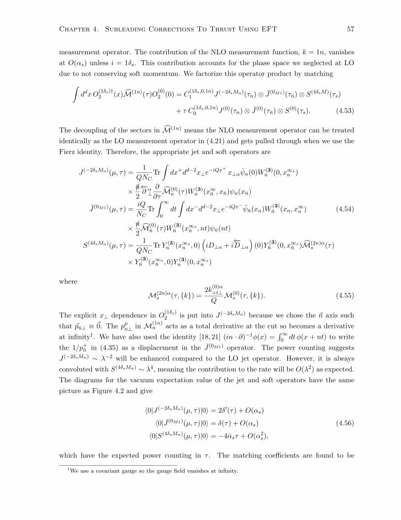
Chapter 4. Subleading Corrections To Thrust Using EFT 57
measurement operator. The contribution of the NLO measurement function, k = 1n, vanishes
at O(αs) unless i = 1δs. This contribution accounts for the phase space we neglected at LO
due to not conserving soft momentum. We factorize this operator product by matching∫ddxO
(1δs)†2 (x)M(1n)(τ)O
(0)2 (0) = C
(1δs,0,1n)1 J (−2δsMn)(τn)⊗ J (0M1)(τn)⊗ S(4δsM)(τs)
+ τ C(1δs,0,1n)0 J (0)(τn)⊗ J (0)(τn)⊗ S(0)(τs). (4.53)
The decoupling of the sectors in M(1n) means the NLO measurement operator can be treated
identically as the LO measurement operator in (4.21) and gets pulled through when we use the
Fierz identity. Therefore, the appropriate jet and soft operators are
J (−2δsMn)(µ, τ) =1
QNCTr
∫dx+dd−2x⊥e
−iQx+x⊥αψn(0)W (3)
n (0, x∞sn )
× /n
2
←−∂ α⊥
∂
∂τM(0)
n (τ)W (3)n (x∞n , xn)ψn(xn)
J (0M1)(µ, τ) =iQ
NCTr
∫ ∞0
dt
∫dx−dd−2x⊥e
−iQx−ψn(xn)W(3)n (xn, x
∞n ) (4.54)
× /n
2M(0)
n (τ)W(3)n (x∞s
n , nt)ψn(nt)
S(4δsMn)(µ, τ) =1
QNCTrY (3)
n (x∞sn , 0)
(iD⊥α + i
←−D⊥α
)(0)Y
(3)n (0, x∞s
n )M(2n)αs (τ)
× Y (3)n (x∞s
n , 0)Y (3)n (0, x∞s
n )
where
M(2n)αs (τ, {k}) =
2k(0)α+t⊥QM(0)
s (τ, {k}). (4.55)
The explicit x⊥ dependence in O(1δs)2 is put into J (−2δsMn) because we chose the ~n axis such
that ~pn⊥ ≡ ~0. The pµn⊥ in M(1n)n acts as a total derivative at the cut so becomes a derivative
at infinity†. We have also used the identity [18, 21] (in · ∂)−1φ(x) =∫∞
0 dt φ(x + nt) to write
the 1/p+n in (4.35) as a displacement in the J (0M1) operator. The power counting suggests
J (−2δsMn) ∼ λ−2 will be enhanced compared to the LO jet operator. However, it is always
convoluted with S(4δsMn) ∼ λ4, meaning the contribution to the rate will be O(λ2) as expected.
The diagrams for the vacuum expectation value of the jet and soft operators have the same
picture as Figure 4.2 and give
〈0|J (−2δsMn)(µ, τ)|0〉 = 2δ′(τ) +O(αs)
〈0|J (0M1)(µ, τ)|0〉 = δ(τ) +O(αs) (4.56)
〈0|S(4δsMn)(µ, τ)|0〉 = −4αsτ +O(α2s),
which have the expected power counting in τ . The matching coefficients are found to be
†We use a covariant gauge so the gauge field vanishes at infinity.

Chapter 4. Subleading Corrections To Thrust Using EFT 58
C(1δs,0,1Mn)1 (µ) = 1 + O(αs) and C
(1δs,0,1Mn)0 (µ) = 0 + O(α2
s) and the contribution from this
operator can be written in the factorized form of (4.39) with hard functions
H(1δs,0,1Mn)1 (µ) = 1 +O(αs)
H(1δs,0,1Mn)0 (µ) = 0 +O(α2
s). (4.57)
This example shows how the decoupling of the measurement operators makes it straightforward
to factorize their contribution.
The factorization of the rest of the subleading dijet and measurement operators follows in
the same way as the above examples. The explicit decoupling of the sectors makes finding
the jet and soft operators a matter of using the Fierz identity to separate spinor and colour
indices. The required jet and soft operators are written in Section 4.7. These operators are
generalizations of the LO operators found in Section 4.3. The matching coefficients are found
by comparing the vacuum expectation values of (4.38). These matrix elements are pictured
in Figure 4.4 of Section 4.7 and their values are shown in Table 4.1 of the Appendix. The
appropriate matching coefficients are shown in Table 4.2. Combining the results of this Table,
we find the O(αsτ) rate is
R(τ) = 1 + αs
(−2 ln2 τ − 3 ln τ +
π2
3− 1 + τ(2 ln τ − 4)
)O(α2
s, τ2). (4.58)
We can compare these results with those found using perturbative QCD in [44]. Although the
results in [44] are for the exclusive two-jet rate using the JADE algorithm, the O(αs) QCD
phase space is the same as the phase space for thrust, as mentioned above. Therefore, the
full O(αs) result calculated in [44] can be compared to (4.58). Summing the τ ln τ ’s requires
renormalizing the jet and soft operators, which we do not do here.
4.5 Conclusion
We have shown how to systematically calculate the O(τ) corrections to the thrust rate in the
perturbative regime using SCET. The rate was factorized and written as the convolution of
the vacuum expectation value of jet and soft operators. Each operator has consistent power
counting and depends on a different scale associated with the rate. The appropriate jet and
soft operators are found in this work, as well as the matching coefficients. The O(αsτ) rate was
calculated and reproduced the rate found using perturbative QCD.
The rate was factorized by matching the QCD currents and measurement operators onto
SCET dijet and measurement operators, which in the formulation of [26], explicitly decouple
the n-collinear, n-collinear, and soft degrees of freedom. The non-local product of the dijet
and measurement operators were then matched onto jet and soft operators that separately
describe each of these degrees of freedom. The approach illustrated here can be applied to

Chapter 4. Subleading Corrections To Thrust Using EFT 59
other jet observables to calculate subleading corrections. We are currently exploring subleading
corrections to the continuous angularity observables of which thrust is an example.
4.6 Appendix: Dijet Operators
The LO dijet operator was given in (4.7). In this section we write the NLO and N2LO dijet
operators necessary for calculating the O(αsτ) thrust rate. They are found by following the
SCET formulation of [26]. The NLO corrections are described in [26] and in chapter 3 along
with their matching coefficients and Feynman rules. We also require the operators describing
N2LO corrections and do so in the same way as NLO operators.
The operators describing the N2LO corrections to the n-collinear sector are
O(2an)2 (x) =
[ψn(xn)PnΓin ·D(xn)W (3)
n (xn, x∞n )] [Y (3)n (x∞s
n , 0)Y(3)n (0, x∞s
n )]
×[W
(3)n (x∞n , xn)Pnψn(xn)
]O
(2bn)2 (x) = −i
∫ ∞0
dt
[ψn(xn + tn)i
←−/D⊥(xn + tn)
/n
2Γ/n
2W (3)n (xn + tn, xn)
×i /D⊥(xn)W (3)n (xn, x
∞n )] [Y (3)n (x∞s
n , 0)Y(3)n (0, x∞s
n )] [W
(3)n (x∞n , xn)ψn(xn)
]O
(2An)2 (x) = −i
∫ ∞0
dt[ψn(xn)PnW
(3)n (xn, xn + tn)Γgσ⊥αβG
αβn (xn + tn) (4.59)
× W (3)n (xn + tn, x∞n )
] [Y (3)n (x∞s
n , 0)Y(3)n (0, x∞s
n )] [W
(3)n (x∞n , xn)Pnψn(xn)
]O
(2δn)2 (x) = Q
[ψn(xn)PnΓ
(n ·D + n ·
←−D)
(xn)W (3)n (xn, x
∞n )] [Y (3)n (x∞s
n , 0)Y(3)n (0, x∞s
n )]
×[x−W
(3)n (x∞n , xn)Pnψn(xn)
]with matching coefficients
C(2an)2 = −1
2+O(αs) C
(2bn)2 = −1 +O(αs)
C(2An)2 =
1
2+O(αs) C
(2δn)2 = 1 +O(αs). (4.60)
We use the same notation as in [26] and chapter 3. The Q in O(2δn)2 is required because of the

Chapter 4. Subleading Corrections To Thrust Using EFT 60
definition in (4.6). The operators describing corrections to the n-collinear sector are
O(2an)2 (x) =
[ψn(xn)PnW
(3)n (xn, x
∞n )] [Y (3)n (x∞s
n , 0)Y(3)n (0, x∞s
n )]
×[W
(3)n (x∞n , xn)Γin ·D(xn)Pnψn(xn)
]O
(2bn)2 (x) = −i
∫ ∞0
dt[ψn(xn)W (3)
n (xn, x∞n )] [Y (3)n (x∞s
n , 0)Y(3)n (0, x∞s
n )]
×[W
(3)n (x∞n , xn)i
←−/D⊥(xn)W
(3)n (xn, xn + tn)
/n
2Γ/n
2i /D(xn + tn)ψn(xn + tn)
]O
(2An)2 (x) = −i
∫ ∞0
dt[ψn(xn)PnW
(3)n (xn, x
∞n )] [Y (3)n (x∞s
n , 0)Y(3)n (0, x∞s
n )]
×[W
(3)n (x∞n , xn + tn)gGαβn (xn + tn)σ⊥αβΓPnW
(3)n (xn + tn, xn)ψn(xn)
]O
(2δn)2 (x) = Q
[x+ψn(xn)PnW
(3)n (xn, x
∞n )] [Y (3)n (x∞s
n , 0)Y(3)n (0, x∞s
n )]
×[W
(3)n (x∞n , xn)Γ
(n ·D + n ·
←−D)
(xn)Pnψn(xn)]
(4.61)
with matching coefficients the same as their n-collinear counterparts. The intuitive picture
of the operators in (4.59) and (4.61) is similar to the pictures presented in [26]. The N2LO
corrections for soft gluon emission are
O(2Ans)2 (x) = −i
∫ ∞0
dt[ψn(xn)PnW
(3)n (xn, x
∞n )]
×[Y (3)n (x∞s
n , tn)gσµνGµνs (tn)Y (3)
n (tn, 0)ΓY(3)n (0, x∞s
n )] [W
(3)n (x∞n , xn)Pnψn(xn)
]O
(2Ans)2 (x) = −i
∫ ∞0
dt[ψn(xn)PnW
(3)n (xn, x
∞n )]
×[Y (3)n (x∞s
n , 0)ΓY(3)n (0, tn)gσµνG
µνs (tn)Y
(3)n (tn, x∞s
n )] [W
(3)n (x∞n , xn)Pnψn(xn)
](4.62)
with matching coefficients
C(2Ans)2 = C
(2Ans)2 =
1
2+O(αs). (4.63)
The corrections from the expansion of the momentum conserving delta function are described

Chapter 4. Subleading Corrections To Thrust Using EFT 61
by
O(2δs+)2 (x) = Q
[x+ψn(xn)PnΓW (3)
n (xn, x∞n )] [Y (3)n (x∞s
n , 0)(n ·D + n ·
←−D)Y
(3)n (0, x∞s
n )]
×[W
(3)n (x∞n , xn)Pnψn(xn)
]O
(2δs−)2 (x) = Q
[ψn(xn)PnΓW (3)
n (xn, x∞n )] [Y (3)n (x∞s
n , 0)(n ·D + n ·
←−D)Y
(3)n (0, x∞s
n )]
×[x−W
(3)n (x∞n , xn)Pnψn(xn)
]O
(2δs⊥)2 (x) =
Q
2
[x⊥αx⊥βψn(xn)PnΓW (3)
n (xn, x∞n )]
×[Y (3)n (x∞s
n , 0)(Dα⊥D
β⊥ +←−Dβ⊥←−Dα⊥
)Y
(3)n (0, x∞s
n )] [W
(3)n (x∞n , xn)Pnψn(xn)
]O
(2δcsn)2 (x) = −i
∫ ∞0
dt[x⊥µψn(xn)PnΓi
←−Dν⊥(xn)W (3)
n (xn, x∞n )]
(4.64)
×[Y (3)n (x∞s
n , tn)i←−D⊥ν(tn)Y (3)
n (tn, 0)(Dµ⊥ +←−Dµ⊥)(0)Y
(3)n (0, x∞s
n )]
×[W
(3)n (x∞n , xn)Pnψn(xn)
]O
(2δcsn)2 (x) = −i
∫ ∞0
dt[x⊥µψn(xn)PnW
(3)n (xn, x
∞n )]
×[Y (3)n (x∞s
n , 0)(Dµ⊥ +←−Dµ⊥)(0)Y
(3)n (0, tn)iD⊥ν(tn)Y
(3)n (tn, x∞s
n )]
×[W
(3)n (x∞n , xn)iDν⊥(xn)ΓPnψn(xn)
]with matching coefficients
C(2δs+)2 = C
(2δs−)2 = 1 +O(αs) C
(2δs⊥)2 = 1 +O(αs)
C(2δcsn)2 = C
(2δcsn)2 = −2 +O(αs). (4.65)
We do not require the N2LO corrections from soft quark emission for an N2LO calculation.
As expected, the subleading operators can be written as separate n-collinear, n-collinear,
and soft pieces. The Feynman rules for the LO and NLO operators at O(αs) were shown in [26].
For the sake of brevity, we do not show the N2LO Feynman rules here. We are only concerned
with vector currents in the above calculations, so Γ = γµ.
4.7 Appendix: Jet and Soft Operators
The jet and soft operators are found by doing the matching in (4.38). It is convenient to use
the basis {1, γα⊥, γ5, σ
αβ⊥ ,
[/n
2,/n
2
], γα⊥γ5,
/n
2,/n
2,/n
2γα⊥,
/n
2γα⊥,
/n
2γ5,
/n
2γ5
}(4.66)

Chapter 4. Subleading Corrections To Thrust Using EFT 62
(a) 〈0|J(08)|0〉
snxn + tn
(b) 〈0|J(2e)|0〉
tnsn
(c) 〈0|S(2dns)|0〉 (d) 〈0|S(08)|0〉
Figure 4.4: Diagrams for the operators describing a soft quark and the quark and anti-quark inthe same sector. The double dashed lines represent Wilson lines in the adjoint representation.Reverse the fermion arrows for 〈0|J (2f)|0〉. The filled boxes highlight a Wilson line changingrepresentation.
for the Dirac matrices. We have defined γµ⊥ = gµν⊥ γν and σµν⊥ = i2 [γµ⊥, γ
ν⊥] where gµν⊥ = gµν −
(nµnν + nν nµ)/2. For use later, we aslo define εαβ⊥ = nµnνεαβµν . The jet and soft operators
will be parity even scalars due to only considering vector currents.
The leading order jet operators required at O(αs) are
J (0)(µ, τ) =1
NCTr
∫dx+dd−2x⊥e
−iQx+ψn(0)W (3)
n (0, x∞sn )
/n
2M(0)
n (τ)
×W (3)n (x∞n , xn)ψn(xn)
J (08)(µ, τ) =gαβ⊥ nµnνQNC
∫dx+dd−2x⊥e
−iQx+Gµαan (0)W (8)
nab(0, x∞s
n )M(0)n (τ) (4.67)
×W (8)n
ba(x∞n , xn)Gνβan (xn)
J (0δn)(µ, τ) =Q
NCTr
∫dx+dd−2x⊥e
−iQx+x+ψn(0)W (3)
n (0, x∞sn )
/n
2M(0)
n (τ)
×W (3)n (x∞n , xn)ψn(xn) (4.68)
J (0cnsδs)(µ, τ) =1
NCTr
∫dx+dd−2x⊥e
−iQx+x⊥αψn(0)
←−Dα⊥(0)W (3)
n (0, x∞sn )
/n
2M(0)(τ)
×W (3)n (x∞n , xn)ψn(xn).
Although J (0cnsδs) has a D⊥ suppression, there is an enhancement by an explicit x⊥ so the
operator is LO. The vacuum expectation value of the operator J (08) is shown in Figure 4.4a.
The other operators have the same diagrams as Figure 4.2 with the appropriate derivative
insertions. The Q’s are introduced by dimensional analysis. There are also the enhanced jet

Chapter 4. Subleading Corrections To Thrust Using EFT 63
operators
J (−2δs)(µ, τ) =Q2
NCTr
∫dx+dd−2x⊥e
−iQx+(x⊥)2ψn(0)W (3)
n (0, x∞sn )
/n
2M(0)
n (τ)
×W (3)n (x∞n , xn)ψn(xn) (4.69)
J (−2δsMn)(µ, τ) =1
NCTr
∫dx+dd−2x⊥e
−iQx+x⊥αψn(0)W (3)
n (0, x∞sn )
/n
2
←−∂ α⊥Q
∂
∂τM(0)
n (τ)
×W (3)n (x∞n , xn)ψn(xn)
J (−2M2nb)(µ, τ) =
1
NCTr
∫dx+dd−2x⊥e
−iQx+ψn(0)W (3)
n (0, x∞sn )
/n
2
n ·←−∂
Q
∂
∂τM(0)
n (τ)
×W (3)n (x∞n , xn)ψn(xn)
where the derivatives act at the cut. These operators are always associated with O(λ4) soft
operators so do not give an enhancement to the thrust rate. We have neglected the contribution
from M(−2na) because it vanishes at O(αs). The required N2LO jet operators are
J (2abn)(µ, τ) =1
Q2NCTr
∫dx+dd−2x⊥e
−iQx+ψn(0)Dα
⊥(0)W (3)n (0, x∞s
n )/n
2M(0)
n (τ)
×W (3)n (x∞n , xn)D⊥α(xn)ψn(xn)
J (2e)(µ, τ) =g2
QNCTr
∫ ∞0
dsdt
∫dx+dd−2x⊥e
−iQx+W (8)n
ab(x∞n , xn + tn)
× ψn(xn)W (3)n (xn, xn + tn)γµ⊥γ⊥α
/n
2T bψn(xn + tn)M(0)
n (τ)
× ψn(sn)T b/n
2γ⊥αγ⊥µW
(3)n (sn, 0)ψn(0)W (8)
nba(sn, x∞s
n )
J (2f)(µ, τ) =g2
QNCTr
∫ ∞0
dsdt
∫dx+dd−2x⊥e
−iQx+W (8)n
ab(x∞n , xn + tn)ψn(xn + tn)T b
×W (3)n (xn + tn, xn)
/n
2γα⊥γ
µ⊥ψn(xn)M(0)
n (τ)
× ψn(0)γ⊥µγ⊥α/n
2W (3)n (0, sn)T bψn(sn)W (8)
nba(tn, x∞s
n )
J (2an)(µ, τ) =1
QNCTr
∫dx+dd−2x⊥e
−iQx+ψn(0)in ·D(0)W (3)
n (0, x∞sn )
/n
2M(0)
n (τ)
×W (3)n (x∞n , xn)ψn(xn)
J (2An)(µ, τ) =1
QNCTr
∫ ∞0
dt
∫dx+dd−2x⊥e
−iQx+ψn(0)W (3)
n (0, tn)gεαβ⊥ Gαβn (tn)
×W (3)n (tn, x∞s
n )/n
2γ5M(0)
n (τ)W (3)n (x∞n , xn)ψn(xn)
J (2δn)(µ, τ) =1
NCTr
∫dx+dd−2x⊥e
−iQx+ψn(0)W (3)
n (0, x∞sn )
/n
2M(0)
n (τ)
×W (3)n (x∞n , xn)
(in ·←−D + in ·D
)(xn)ψn(xn) (4.70)

Chapter 4. Subleading Corrections To Thrust Using EFT 64
and their hermitian conjugates. The vacuum expectation value of J (2abn) was pictured in Figure
4.3. Although J (2e) and J (2f) look complicated, they have simple diagrams shown in Figure
4.4b. The γ5 in J (2An) is necessary because εαβ⊥ is parity odd. The vacuum expectation value
of these operators are shown in Table 4.1a.
The J operators are similar to the J operators. The leading order operators are
J (0)(µ, τ) =1
NCTr
∫dx−dd−2x⊥e
−iQx−ψn(xn)W(3)n (xn, x
∞n )
/n
2M(0)
n (τ)W(3)n (x∞s
n , 0)ψn(0)
J (08)(µ, τ) =gαβ⊥ nµnν
Q
∫dx−dd−2x⊥e
−iQx−Gµαan (xn)W(8)n
ab(xn, x∞n )M(0)
n (τ)
×W (8)n
ba(x∞sn , 0)Gνβan (0)
J (0M1)(µ, τ) =iQ
NCTr
∫ ∞0
dt
∫dx−dd−2x⊥e
−iQx−ψn(xn)W(3)n (xn, x
∞n )
/n
2M(0)
n (τ)
×W (3)n (x∞s
n , tn)ψn(tn) (4.71)
J (0M2)(µ, τ) =iQ2
NCTr
∫ ∞0
dt
∫ ∞0
ds
∫dx−dd−2x⊥e
−iQx−ψn(xn)W(3)n (xn, x
∞n )
/n
2M(0)
n (τ)
×W (3)n (x∞s
n , (t+ s)n)ψn((t+ s)n)
J (0δn)(µ, τ) =iQ
NCTr
∫dx−dd−2x⊥e
−iQx−x−ψn(xn)W(3)n (xn, x
∞n )
/n
2M(0)
n (τ)
×W (3)n (x∞s
n , 0)ψn(0).
There is only one enhanced operator that needs to be considered
J (−2Mnb)(µ, τ) =
1
NCTr
∫dx−dd−2x⊥e
−iQx−ψn(xn)W(3)n (xn, x
∞n )
/n
2
in ·←−∂
Q
∂
∂τM(−2nb)
n (τ)
×W (3)n (x∞s
n , 0)ψn(0). (4.72)
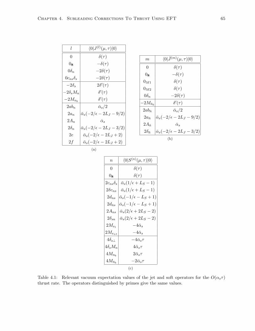
Chapter 4. Subleading Corrections To Thrust Using EFT 65
l 〈0|J (l)(µ, τ)|0〉
0 δ(τ)
08 −δ(τ)
0δn −2δ(τ)
0cnsδs −2δ(τ)
−2δs 2δ′(τ)
−2δsMn δ′(τ)
−2Mnb δ′(τ)
2abn αs/2
2an αs(−2/ε− 2LJ − 9/2)
2An αs
2δn αs(−2/ε− 2LJ − 3/2)
2e αs(−2/ε− 2LJ + 2)
2f αs(−2/ε− 2LJ + 2)
(a)
m 〈0|J (m)(µ, τ)|0〉
0 δ(τ)
08 −δ(τ)
0M1 δ(τ)
0M2 δ(τ)
0δn −2δ(τ)
−2Mnb δ′(τ)
2abn αs/2
2an αs(−2/ε− 2LJ − 9/2)
2An αs
2δn αs(−2/ε− 2LJ − 3/2)
(b)
n 〈0|S(n)(µ, τ)|0〉
0 δ(τ)
08 δ(τ)
2cnsδs αs(1/ε+ LS − 1)
2δcns αs(1/ε+ LS − 1)
2dns αs(−1/ε− LS + 1)
2dns αs(−1/ε− LS + 1)
2Ans αs(2/ε+ 2LS − 2)
2δsn αs(2/ε+ 2LS − 2)
2Ms1 −4αs
2Ms+t −4αs
4δs⊥ −4αsτ
4δsMn 4αsτ
4Mnb 2αsτ
4Mnb −2αsτ
(c)
Table 4.1: Relevant vacuum expectation values of the jet and soft operators for the O(αsτ)thrust rate. The operators distinguished by primes give the same values.

Chapter 4. Subleading Corrections To Thrust Using EFT 66
The N2LO operators are
J (2abn)(µ, τ) =1
QNCTr
∫dx−dd−2x⊥e
−iQx−ψn(xn)iDα⊥W
(3)n (xn, x
∞sn )
/n
2M(0)
n (τ)
×W (3)n (x∞n , xn)iD⊥α(xn)ψn(0)
J (2an)(µ, τ) =1
QNCTr
∫dx−dd−2x⊥e
−iQx−ψn(xn)W(3)n (xn, x
∞sn )
/n
2M(0)
n (τ)
×W (3)n (x∞n , 0)in ·
←−D(0)ψn(xn) (4.73)
J (2An)(µ, τ) =1
QNCTr
∫ ∞0
dt
∫dx+dd−2x⊥e
−iQx+ψn(xn)W
(3)n (xn, x
∞n )γ5
/n
2M(0)
n (τ)
×W (3)n (x∞n , tn)gεαβ⊥ Gαβn (tn)W (3)
n (tn, 0)ψn(0)
J (2δn)(µ, τ) =1
NCTr
∫dx−dd−2x⊥e
−iQx−ψn(xn)(in ·←−D + in ·D
)(xn)W
(3)n (xn, x
∞sn )
/n
2
× M(0)n (τ)W
(3)n (x∞n , 0)ψn(0)
The diagrams are similar to those found for the J operators. For example, J (08) is the horizontal
reflection of Figure 4.4a. The vacuum expectation values of these operators are shown in Table
4.1b. The difference in the required J operators compared to the J operators is because we
have chosen the ~n axis to be anti-parallel to the n-collinear sector.
The leading order soft operators are
S(0)(µ, τ) =1
NCTrY
(3)n (x∞s
n , 0)Y (3)n (0, x∞s
n )M(0)s (τ)Y (3)
n (x∞sn , 0)Y
(3)n (0, x∞s
n ) (4.74)
S(08)(µ, τ) =1
N2C
TrY(8)n
ab(x∞sn , 0)Y (8)
nbc(0, x∞s
n )M(0)s (τ)Y (8)
ncd(x∞s
n , 0)Y(8)n
da(0, x∞sn )
which only differ in the representation of the Wilson lines. The vacuum expectation value of

Chapter 4. Subleading Corrections To Thrust Using EFT 67
S(08) is pictured in Figure 4.4d. The N2LO operators are
S(2cnsδs)(µ, τ) =i
QNCTr
∫ ∞0
dtY(3)n (x∞s
n , 0)(i←−Dα⊥ + iDα
⊥
)(0)Y (3)
n (0, x∞sn )M(0)
s (τ)
× Y (3)n (x∞s
n , tn)i←−Dα⊥(tn)Y (3)
n (tn, 0)Y(3)n (0, x∞s
n )
S(2δcns)(µ, τ) =QNC
Tr
∫ ∞0
dtY(3)n (x∞s
n , 0)(i←−Dα⊥ + iDα
⊥
)(0)Y (3)
n (0, tn)D⊥α(tn)
× Y (3)n (tn, x∞s
n )M(0)s (τ)Y (3)
n (x∞sn , 0)Y
(3)n (0, x∞s
n )
S(2dns)(µ, τ) =g2
QN2C
Tr
∫ ∞0
dsdt Y (8)n
ab(x∞sn , sn)ψs(sn)T bY (3)
n (sn, 0)
× Y (3)n (0, x∞s
n )/n
2M(0)
s (τ)Y(3)n (x∞s
n , 0)Y (3)n (0, tn)T cψs(tn)Y (8)
nca(tn, x∞s
n )
S(2dns)(µ, τ) =g2
QN2C
Tr
∫ ∞0
dsdt Y(8)n
ab(x∞sn , sn)ψs(sn)T bY
(3)n (sn, 0)
× Y (3)n (0, x∞s
n )/n
2M(0)
s (τ)Y (3)n (x∞s
n , 0)Y(3)n (0, tn)T cψs(tn)Y
(8)n
ca(tn, x∞sn )
S(2Ans)(µ, τ) =gnαnβQNC
Tr
∫ ∞0
dt Y(3)n (x∞s
n , 0)Y (3)n (0, tn)Gαβs (tn)Y (3)
n (tn, x∞sn )M(0)
s (τ)
× Y (3)n (x∞s
n , 0)Y(3)n (0, x∞s
n )
S(2Ans)(µ, τ) =gnαnβQNC
Tr
∫ ∞0
dt Y(3)n (x∞s
n , tn)Gαβs (tn)Y(3)n (tn, 0)Y (3)
n (0, x∞sn )M(0)
s (τ)
× Y (3)n (x∞s
n , 0)Y(3)n (0, x∞s
n )
S(2δsn)(µ, τ) =1
QNCTrY
(3)n (x∞s
n , 0)(in ·←−D + in ·D
)(0)Y (3)
n (0, x∞sn )M(0)
s (τ)
× Y (3)n (x∞s
n , 0)Y(3)n (0, x∞s
n )
S(2δsn)(µ, τ) =1
QNCTrY
(3)n (x∞s
n , 0)(in ·←−D + in ·D
)(0)Y (3)
n (0, x∞sn )M(0)
s (τ)
× Y (3)n (x∞s
n , 0)Y(3)n (0, x∞s
n ) (4.75)
There are also N2LO operators involving the measurement function expansion that we write as
S(2Mi)(µ, τ) =1
NCTrY
(3)n (x∞s
n , 0)Y (3)n (0, x∞s
n )M(2i)s (τ)Y (3)
n (x∞sn , 0)Y
(3)n (0, x∞s
n ) (4.76)
where
M(s1)s (τ, {k}) =
2(~k(0)+t⊥)2
Q2
∂
∂τM(0)
s (τ, {k})
M(s+t)s (τ, {k}) =
p+n n · k
(2)+t
Q2
∂
∂τM(0)
s (τ, {k}) (4.77)
where the p+n cancels in the definition of k
(2)+t in (4.31). The contribution from the other
measurement operators in (4.36) vanish at O(αs).

Chapter 4. Subleading Corrections To Thrust Using EFT 68
There are also N4LO operators that contribute to the N2LO rate due to convoluting with
enhanced jet operators. These operators are
S(4δs⊥)(µ, τ) =1
NCTrY
(3)n (x∞s
n , 0)(←−Dα⊥←−D⊥α +Dα
⊥D⊥α
)Y (3)n (0, x∞s
n )M(0)s (τ)
× Y (3)n (x∞s
n , 0)Y(3)n (0, x∞s
n )
S(4δsMn)(µ, τ) =1
QNCTrY (3)
n (x∞sn , 0)(iDα
⊥ + i←−Dα⊥)Y
(3)n (0, x∞s
n )M(2n)αs (τ)
× Y (3)n (x∞s
n , 0)Y (3)n (0, x∞s
n ) (4.78)
S(4Mi)(µ, τ) =1
NCTrY
(3)n (x∞s
n , 0)Y (3)n (0, x∞s
n )M(4i)s (τ)Y (3)
n (x∞sn , 0)Y
(3)n (0, x∞s
n )
where
M(4nb)s (τ, {k}) =
−(~k(0)+t⊥)2
Q2M(0)
s (τ, {k})
M(4nb)s (τ, {k}) =
(~k(0)+t⊥)2
Q2M(0)
s (τ, {k}). (4.79)
The vacuum expectation value of the soft operators are shown in Table 4.1c.
The operators in Section 4.6 are matched onto combinations of the operators in this section.
The matching coefficients are found by taking the vacuum expectation value of both sides of
(4.38) and are shown in Table 4.2. Using this Table and Table 4.1 the O(αsτ) rate in (4.58)
can be calculated.

Chapter 4. Subleading Corrections To Thrust Using EFT 69
(i, j, k) (l,m, n) C(i,j,k)1 H
(i,j,k)1 R(τ)
(1an, 1bn, 0) (2abn, 0, 0) −1 +1 αsτ/2
(1bn, 1an, 0) (2ab†n, 0, 0) −1 +1 αsτ/2
(2an, 0, 0) (2an, 0, 0) 1 −1/2 αsτ(−1/ε− LJ − 9/4)
(0, 2an, 0) (2a†n, 0, 0) 1 −1/2 αsτ(−1/ε− LJ − 9/4)
(2An, 0, 0) (2An, 0, 0) −1/2 −1/4 −αsτ/4(0, 2An, 0) (2A†n, 0, 0) −1/2 −1/4 −αsτ/4(2δn, 0, 0) (2δn, 0δn, 0) 1 1 αs(4/ε+ 4LJ + 7)
(1en, 1en, 0) (2e, 08, 08) −1/2 −1/2 αsτ(−1/ε− LJ − 2)
(1fn, 1fn, 0) (2f, 08, 08 −1/2 −1/2 αsτ(−1/ε− LJ − 2)
(1an, 1bn, 0) (0, 2abn, 0) −1 +1 αsτ/2
(1bn, 1an, 0) (0, 2ab†n, 0) −1 +1 αsτ/2
(2an, 0, 0) (0, 2an, 0) 1 −1/2 αsτ(−1/ε− LJ − 9/4)
(0, 2an, 0) (0, 2a†n, 0) 1 −1/2 αsτ(−1/ε− LJ − 9/4)
(2An, 0, 0) (0, 2An, 0) −1/2 −1/4 −αsτ/4(0, 2An, 0) (0, 2A†n, 0) −1/2 −1/4 −αsτ/4(2δn, 0, 0) (2δn, 0δn, 0) 1 1 αs(4/ε+ 4LJ + 7)
(1δs, 1cns, 0) (0cnsδs, 0, 2cnsδs) 1/2 1 αsτ(−2/ε− 2LS − 2)
(2δcsn, 0, 0) (0cnsδs, 0, 2δcns) 1/2 1 αsτ(−2/ε− 2LS − 2)
(1dns, 1dns, 0) 08, 0, 2dns) 1 1 αsτ(1/ε+ LS + 1)
(1dns, 1dns, 0) (08, 0, 2dns) 1 1 αsτ(1/ε+ LS + 1)
(2Ans, 0, 0) (0, 0, 2Ans) 1 1/2 αsτ(1/ε+ LS + 1)
(0, 2Ans, 0) (0, 0, 2A†ns) 1 1/2 αsτ(1/ε+ LS + 1)
(2Ans, 0, 0) (0, 0, 2Ans) 1 1/2 αsτ(1/ε+ LS + 1)
(0, 2Ans, 0) (0, 0, 2A†ns) 1 1/2 αsτ(1/ε+ LS + 1)
(2δs−, 0, 0) (0, 0δn, 2δs−) 1 1 αsτ(−4/ε− 4LS − 4)
(2δs⊥, 0, 0) (−2δs, 0, 4δs⊥) 1/2 1/2 4αsτ
(1δs, 0, 1n) (−2δsMn, 0M1, 4δsMn) 1 1 4αsτ
(0, 0, 2nb) (−2M2nb , 0M2, 4Mnb) 1 1 −2αsτ
(0, 0, 2nb) (0,−2Mnb , 4Mnb) 1 1 2αsτ
(0, 0, 2s1) (0, 0M , 2Ms1) 1 1 −4αsτ
(0, 0, 2s+t) (0, 0M , 2M+t) 1 1 −4αsτ
(i, j, k) C(i,j,k)0 H
(i,j,k)0 R(τ)
(2δn, 0, 0) −4αs −4αs −4αsτ
(1en, 1en, 0) αs αs αsτ
(1fn, 1fn, 0) αs αs αsτ
(2δn, 0, 0) −4αs −4αs −4αsτ
(1dns, 1dns, 0) −αs −αs −αsτ(1dns, 1dns, 0) −αs −αs −αsτ
(2δs−, 0, 0) 4αs 4αs 4αsτ
Table 4.2: The operators and matching coefficients for the O(αs) factorization. The daggermeans the operator is the hermitian conjugate. At O(αsτ), there is at most one set of subleadingjet and soft operators to be matched onto, so α = 1. The table at the bottom gives the matchingcoefficients for the last line of (4.38). Values of the hard functions defined in (4.40), and thecontribution to R(τ) are also given.
Chapter 5
Renormalization of Subleading Dijet
Operators in Soft-Collinear Effective
Theory
In this chapter we calculate the anomalous dimensions of the next-to-leading order dijet oper-
ators in the SCET formulation of Chapter 3. We introduce a small gluon mass to regulate the
infrared divergences of the individual loop diagrams in order to properly extract the ultraviolet
divergences. We discuss this choice of infrared regulator and contrast it with the δ-regulator.
Our results can be used to increase the theoretical precision of the thrust distribution. The
text in this chapter is reproduced in [48].
5.1 Introduction
Perturbative calculations of jet observables involve multiple scales. In the kinematic region
where all the scales are much greater than ΛQCD but the ratio of these scales is small, often
called the “tail” region, the rate is perturbative in both the strong coupling constant αs and
the ratio of the scales involved. However, the rate includes large logarithms of the ratio of
these scales at each order in perturbation theory. These large logarithms limit the precision
of theoretical predictions. EFT techniques provide a framework to sum the terms enhanced
by the logarithms using renormalization group equations (RGE). This framework also contains
a systematic procedure for including higher order effects in the small ratio of scales using
subleading operators, allowing for logarithms suppressed by this small ratio to be summed in
addition to those at leading order in the ratio. These techniques can be used to improve the
precision of the theoretical predictions. In this chapter we renormalize the next-to-leading order
dijet operators in SCET with the purpose of using the RGE to sum the logarithms suppressed
by the ratio of scales. We will use the SCET operators introduced in the formulation of [26,40],
in which the QCD dynamics of jets are described by multiple decoupled copies of QCD, and the
70
Chapter 5. Renormalization of Subleading Dijet Operators in SCET 71
EFT expansion only enters in the external currents. Our results are useful for any observable
requiring dijet operators; however, we will use the concrete example of the thrust rate to
illustrate their usefulness.
Thrust [49] is a useful jet shape observable for precision studies of high energy collisions, in
particular for measuring αs(MZ) from LEP data∗. Thrust is defined as
τ =1
Q
∑i∈X
min(Ei + ~t · ~pi, Ei − ~t · ~pi
), (5.1)
where X is the final state, Q is the total energy, and ~t is chosen to maximize the sum. The
integrated rate of the differential thrust distribution is defined by
R(τ) =1
σ0
∫ τ
0dτ ′
dσ
dτ ′, (5.2)
where the Born rate is σ0. We will call this the thrust rate in the following. A perturbative
calculation of the thrust rate in the tail region where (ΛQCD/Q)� τ � 1 involves three relevant
scales: the hard scattering scale Q, the intermediate scale√τQ, and the soft scale τQ. The
rate can be written as an expansion R(τ) = R(0)(τ) + τR(1)(τ) + O(τ2) in this region, where
the superscripts refer to the suppression in τ , with R(0) and R(1) referring to O(τ0) and O(τ)
rate respectively. Each of the R(i)(τ) terms in the thrust rate has an expansion in αs of the
form
R(0)(τ) =∑n
∑m≤2n
R(0)nmα
ns lnm(τ),
R(1)(τ) =∑n
∑k≤2n−1
R(1)nkα
ns lnk(τ), (5.3)
where the R(i)nm are O(1) constants and the large logarithms ln τ � 1 are due to the separation
of scales. The highest logarithmic power for the O(τ) rate is suppressed by an additional power
of αs relative to the O(τ0) rate. When αs ln τ ∼ O(1) the O(τ0) rate becomes a divergent sum
in increasing powers of ln τ , spoiling the expansion in αs(Q)� 1. Although the O(τ) rate has
an overall suppression by τ compared to the O(τ0) rate, the rate is similarly a sum in increasing
powers of the logarithm. Therefore, in order to restore a perturbative expansion in αs for both
the O(τ0) and O(τ) rates, the logarithms must be summed.
The O(τ0) thrust rate has already been calculated to N3LL accuracy and included the fixed
order O(τ) rate at O(αs) [51]. In order to increase the theoretical precision in the tail region,
the leading logarithms in the O(τ) rate can become more important than further increasing the
logarithmic accuracy in the O(τ0) rate. Therefore, if the precision of the αs(MZ) measurement
is to be improved, these former contributions to the thrust rate will need to be calculated.
The appropriate EFT for describing thrust is SCET [16–21,24,26]. SCET includes collinear
∗See [50] and previous works by this collaboration.

Chapter 5. Renormalization of Subleading Dijet Operators in SCET 72
and ultrasoft (usoft) fields that reproduce both the highly boosted, and low energy degrees
of freedom that are relevant in the tail region. The expansion parameter of SCET is usually
denoted by λ. For thrust λ ∼√τ , meaning the O(τ) corrections require next-to-next-to-leading
order in λ (N2LO) corrections to the effective theory†. We use a formulation of SCET in which
QCD fields are coupled to Wilson lines [26]. Each of the sectors (usoft and collinear) interact
amongst themselves via QCD, while the interactions between sectors are described by Wilson
lines in appropriate representations. This picture has been shown explicitly to N2LO by doing a
tree-level matching from QCD [40]. We contrast this formulation with the traditional approach
to SCET, which has a Lagrangian expansion and mixes the various sectors [16–21,24].
SCET can sum the large logarithms in (5.3) by factorizing the rate and using the RGE
to run from the hard scale to the soft scale. The QCD operators are first matched onto the
appropriate SCET dijet operators at the hard scale Q. For the O(τ0) rate we use the LO dijet
operators. The O(τ) rate requires the NLO and N2LO dijet operators, which are then run to
the intermediate scale√τQ using the RGE. At the intermediate scale, the dijet operators are
matched onto soft operators with the help of a factorization theorem. The Wilson coefficients
of the soft operators, often called the jet function, are run to the soft scale τQ. The sequence
of matching and running sums the large logarithms in the rate.
Recently, a factorization theorem has been shown for the O(τ) rate [40] that makes this
possible. The appropriate dijet operators and the tree-level matching coefficients were derived,
as well as the appropriate soft operators. By solving the RGE for the operators in [40] the
large logarithms in the O(τ) rate can be summed. In this chapter we begin this process by
calculating the anomalous dimensions of the NLO dijet operators in SCET. Summing all the
logarithms in the O(τ) rate of (5.3) also require the N2LO dijet operators, which we leave for
future work.
To compute the anomalous dimensions of the subleading effective operators we first compute
their counterterms. We regulate using the MS scheme and include a separate infrared (IR)
regulator to ensure the 1/ε poles are ultraviolet (UV) divergences. The decoupling of the
collinear and usoft sectors, manifest in the formulation of [26], means the IR cannot be regulated
using a fermion off-shellness because the usoft sector will not be changed by this regulator. We
identify two possible IR regulators that will regulate the formulation of [26]: the δ-regulator and
a gluon mass. The δ-regulator [52] is similar to off-shellness but also modifies the Feynman rules
of the usoft Wilson lines. Unfortunately, the regulator introduces additional terms that make
the calculation unnecessarily complicated. We will demonstrate this in Section 5.3.1. A gluon
mass does not introduce any additional terms, meaning fewer calculations are needed. However,
this is done at the expense of introducing unregulated divergences in individual diagrams that
only cancel if all the diagrams are added together before integrating. Either choice of regulator
is equivalent since the counterterms do not depend on the IR regulator. We chose to use a
gluon mass.
†Unless otherwise stated, LO, NLO, and N2LO refer to the expansion in λ.

Chapter 5. Renormalization of Subleading Dijet Operators in SCET 73
The rest of the chapter is organized as follows: In Section 5.2 we briefly summarize the
SCET formulation of [26] and write the operators used in this calculation. We note that it
was necessary to generalize the operators of [26] in order to account for the mixing that occurs
under renormalization. In Section 5.3 we discuss our choice of using a gluon mass as an IR
regulator over the δ-regulator. We present the anomalous dimensions for the NLO operators in
Section 5.4 and conclude in Section 5.5.
5.2 SCET and NLO Operators
In the kinematic region where thrust is dominated by collimated jets of light, energetic parti-
cles, SCET is the appropriate description. It is convenient to introduce light-cone coordinates
for describing the momentum of the highly boosted particles. In light-cone coordinates the
momentum is decomposed into two light-like components described by the vectors nµ and nµ
as
pµ = p · nnµ
2+ p · nn
µ
2+ pµ⊥. (5.4)
The vectors nµ and nµ satisfy n2 = 0 = n2 and n · n = 2. A boosted particle with p · n ∼ Q
will be described by n-collinear fields in the effective theory. Similarly, a boosted particle with
p · n ∼ Q will be described by an n-collinear field. The perpendicular momentum of a collinear
particle pµ⊥ ∼ λQ is suppressed compared to the hard scale. We must also include usoft fields
that have no large components of momentum and whose momentum scales like pµ ∼ λ2Q.
We follow the approach of [26] in deriving the NLO SCET dijet operators. Since particles
in the same sector have no large momentum transfers, the interactions within each sector are
governed by QCD. Consequently, the Lagrangian has no expansion in λ and can be written as
LSCET = LnQCD + LnQCD + LusQCD, (5.5)
where LiQCD is the QCD Lagrangian involving only ith-sector fields.‡ The interactions of particles
in different sectors are described by external currents. Since these interactions involve large
momentum transfers, the external currents can be organized into an expansion in λ. When
computing the thrust rate in the limit τ � 1, the relevant external currents are dijet operators,
which can be determined by matching the full QCD current
ψ(x)Γψ(x) = e−iQ(n+n)·x/2
[C
(0)2 O
(0)2 (x) +
1
Q
∑i
∫{dt}C(1i)
2 ({t})O(1i)2 (x, {t}) +O(λ2)
](5.6)
for a general Dirac structure Γ. The phase corresponding to the external momentum has been
pulled out. The superscripts in the dijet operators refer to the suppression in λ and the 1/Q is
included because the subleading operators are higher dimensional. We have introduced a set of
‡The approach of including decoupled copies of QCD for each sector has also been used to study factorizationin QCD [53,54].

Chapter 5. Renormalization of Subleading Dijet Operators in SCET 74
dimensionless shift variables {t} = {Qt} that were not included in [26]; it will become apparent
below that this shift corresponds to a displacement along a light-like direction describing the
position of a derivative insertion. This generalization is needed in order to properly describe
the mixing of operators under renormalization.
The leading order operator in (5.6) is [26]
O(0)2 (x) =
[ψn(xn)W (3)
n (xn, x∞n )] [Y (3)n (x∞n
s , 0)Γ(0)Y(3)n (0, x∞n
s )] [W
(3)n (x∞n , xn)ψn(xn)
],
(5.7)
and its matching coefficient is [45,55]
C(0)2 (µ) = 1 +
αsCF4π
(− ln2 µ2
−Q2− 3 ln
µ2
−Q2− 8 +
π2
6
)(5.8)
where µ is the renormalization scale. The Dirac structure is
Γ(0) = PnΓPn (5.9)
with projectors Pn = (/n/n)/4 and Pn = (/n/n)/4. The subscripts on the fields denote the sector of
the field. Each of the square brackets in (5.7) are independently gauge invariant and corresponds
to a separate sector. The Wilson lines in the R representation
W (R)n (x, y) = P exp
(−ig
∫ n·(y−x)/2
0dsn ·Aan(x+ ns)T aRe
−sε
)
Y (R)n (x, y) = P exp
(−ig
∫ n·(y−x)/2
0dsn ·Aas(x+ ns)T aRe
−sε
), (5.10)
represent a light-like colour source corresponding to the total colour of the other sectors (the
symbol P indicates path-ordering). The ε in the definition above gives the proper iε pole
prescription. The W(R)n and Y
(R)n Wilson lines are defined similarly. The positions in (5.7)
xn = (0, x · n, x⊥) x∞n = (0,∞, x⊥)
xn = (x · n, 0, x⊥) x∞n = (∞, 0, x⊥) (5.11)
x∞ns = (∞, 0, 0) x∞n
s = (0,∞, 0),
come from multipole expanding the total momentum conservation constraint in λ and is needed
to ensure consistent power-counting at each order in λ.
The NLO operators are found by including O(λ) corrections in the interactions between the

Chapter 5. Renormalization of Subleading Dijet Operators in SCET 75
sectors [26]. The operators that describe the modification to the n-collinear sector are
O(1an)2 (x, t) =
[ψn(xn)W (3)
n (xn, xn + nt)iDµ⊥(xn + nt)W (3)
n (xn + nt, x∞n )]
×[Y (3)n (x∞n
s , 0)Γµ(1an)Y(3)n (0, x∞n
s )] [W
(3)n (x∞n , xn)ψn(xn)
]O
(1bn)2 (x, t) =
[ψ(xn)W (3)
n (xn, xn + tn)iDµ⊥(xn + tn)W (3)
n (xn + tn, x∞n )]
×[Y (3)n (x∞n
s , 0)Γµ(1bn)Y(3)n (0, x∞n
s )] [W
(3)n (x∞n , xn)ψn(xn)
]O
(1Bn)2 (x) =
[ψ(xn)W (3)
n (xn, x∞n )i←−∂ µ⊥
](5.12)
×[Y (3)n (x∞n
s , 0)Γµ(1bn)Y(3)n (0, x∞n
s )] [W
(3)n (x∞n , xn)ψn(xn)
]O
(1cn)2 (x, t1, t2) =
[ψn(xn)W (3)
n (xn, xn + t2n)i←−Dµ⊥(xn + t2n)W (3)
n (xn + t2n, x∞n )]
×[Y (3)n (x∞n
s , t1n)i←−Dµ⊥(t1n)Y (3)
n (t1n, 0)Γ(1cn)Y(3)n (0, x∞n
s )]
×[W
(3)n (x∞n , xn)ψn(xn)
]O
(1dn)2 (x, t) =
[ignµG
aµνn⊥ (xn)W (8)
nab(xn, x
∞n )]
×[Y (8)n
bc(x∞ns , tn)ψs(tn)T cY (3)
n (tn, 0)Γν(1dn)Y(3)n (0, x∞n
s )]
×[W
(3)n (x∞n , xn)ψn(xn)
]O
(1en)2 (x, t) =
[ignµG
aµνn⊥ (xn)W (8)
nab(xn, x
∞n )] [Y (3)n
dd(x∞ns , 0)Y
(8)n
dc(0, x∞ns )
]×[W
(8)n
cb(x∞n , xn + tn)ψn(xn + tn)T bΓ(1en)W(3)n (xn + tn, xn)ψn(xn)
]O
(1δ)2 (x) =Q
[ψn(xn)xµ⊥W
(3)n (xn, x
∞n )]
×[Y (3)n (x∞n
s , 0)Γ(1δ)(Dµ⊥ +←−Dµ⊥)(0)Y
(3)n (0, x∞n
s )] [W
(3)n (x∞n , xn)ψn(xn)
],
where the Dirac structures are
Γµ(1an) =PnΓγµ/n
2Γµ(1bn) =
/n
2γµΓPn Γ(1cn) =PnΓPn
Γµ(1dn) =/n
2γµ⊥ΓPn Γµ(1en) =
/n
2γµ⊥ΓPn Γ(1δ) =PnΓPn. (5.13)
The covariant derivative is defined as Dµ(x) = ∂µ − igT aAaµ(x) and only couples the gluon
to the corresponding sector on which it acts. The field strength tensor is defined as igGaµν =
fabc[Abµ, Acν ] where fabc are the SU(3) structure constants. The derivative in the (1Bn) oper-
ator is strictly a partial derivative and not a covariant derivative because we are working in a
covariant gauge where the gauge transformations at infinity vanish. The Q in front of the (1δ)
operator is required dimensionally. The matching coefficients for the operators listed above

Chapter 5. Renormalization of Subleading Dijet Operators in SCET 76
are [26]
C(1an)2 (t) = −δ(t) +O(αs) C
(1bn)2 (t) = δ(t) +O(αs)
C(1Bn)2 = 1 +O(αs) C
(1cn)2 (t2, t1) = 2iθ(t1)δ(t2) +O(αs) (5.14)
C(1dn)2 (t) = −2iθ(t) +O(αs) C
(1en)2 (t) = iθ(t) +O(αs)
C(1δ)2 (t) = 1 +O(αs),
which are all dimensionless. The factors of i ensure the convolution in (5.6) is real.
The NLO operators explicitly decouple the sectors, just as in the LO operator. These
operators differ from the LO operators by a D⊥ insertion at an arbitrary point along a Wilson
line (for example the (1an) operator) or by a change in the field content and Wilson line
representation (for example the (1en) operator). The operators in (5.12) are generalizations of
the NLO operators in [26, 40]. We find the form in (5.12) is necessary to properly renormalize
the operators, since different values of the parameters can mix under renormalization. We have
also slightly changed the definition of the (1bn) operator and included the (1Bn) operator, which
makes the operator basis in (5.12) diagonal under renormalization.
As was done in [26], we can compare the operators in (5.12) with the subleading operators
in other formulations of SCET, such as in [56]. In [56] the subleading heavy-to-light currents
were renormalized. While the dijet and heavy-to-light operators obviously differ in the usoft
and n-collinear sectors, the modifications to the n-collinear sector from the vector currents
and subleading Lagrangian insertions in [56] only differ from the corresponding operators in
(5.12) by the appropriate Dirac structure basis. This will serve as a way for us to compare the
anomalous dimensions we calculate in Section 5.4 with the results of [56].
We find it more convenient to work with the Fourier transformed operators O(i)2 defined as
O(1i)2 (x, u) =
∫dt
(2π)e−iutO
(1i)2 (x, t) = Q
∫dt
(2π)e−iQutO
(1i)2 (x, t)
O(1i)2 (x, u2, u1) =
∫dt2(2π)
dt1(2π)
e−i(t2u2+t1u1)O(1i)2 (x, t2, t1). (5.15)
The matching in (5.6) is written in terms of these operators as∫d{t}C(1i)
2 ({t})O(1i)2 ({t}) =
∫d{u}C(1i)
2 ({u})O(1i)2 ({u}) (5.16)
where
C(1i)2 (u) =
∫dt eiutC
(1i)2 (t)
C(1i)2 (u2, u1) =
∫dt2dt1 e
i(u2 t2+u1 t1)C(1i)2 (t2, t1). (5.17)
The u’s are momentum fractions at the vertex of the external current. For collinear momentum

Chapter 5. Renormalization of Subleading Dijet Operators in SCET 77
0 ≤ u ≤ 1 due to momentum conservation, while for usoft momentum 0 ≤ u <∞ because usoft
momentum is not conserved at the vertex. The Fourier transformation of the NLO operators
are
O(1an)2 (x, u) =
[ψn(xn)δ(u− in · D)iDµ
⊥(xn)W (3)n (xn, x
∞n )]
×[Y (3)n (x∞n
s , 0)Γµ(1an)Y(3)n (0, x∞n
s )] [W
(3)n (x∞n , xn)ψn(xn)
]O
(1bn)2 (x, u) =
[ψ(xn)δ(u− in · D)iDµ
⊥(xn)W (3)n (xn, x
∞n )]
×[Y (3)n (x∞n
s , 0)Γµ(1bn)Y(3)n (0, x∞n
s )] [W
(3)n (x∞n , xn)ψn(xn)
]O
(1cn)2 (x, u2, u1) =
[ψn(xn)δ(u2 − in · D)i
←−Dµ⊥(xn)W (3)
n (xn, x∞n )]
×[Y (3)n (x∞n
s , 0)i←−Dµ⊥(0)δ(u1 − in ·
←−D)Γ(1cn)Y
(3)n (0, x∞n
s )
]×[W
(3)n (x∞n , xn)ψn(xn)
]O
(1dn)2 (x, u) =
[ignµG
aµνn⊥ (xn)W (8)
nab(xn, x
∞n )]
(5.18)
×[Y (8)n
bc(x∞ns , 0)ψs(0)T cδ(u− in ·
←−D)Γν(1dn)Y
(3)n (0, x∞n
s )
]×[W
(3)n (x∞n , xn)ψn(xn)
]O
(1en)2 (x, u) =
[ignµG
aµνn⊥ (xn)W (8)
nab(xn, x
∞n )] [Y (3)n
dd(x∞ns , 0)Y
(8)n
dc(0, x∞ns )
]×[W
(8)n
cb(x∞n , xn)ψn(xn)T bΓ(1en)δ(u− in ·←−D)ψn(xn)
]where Dµ = Dµ/Q is a dimensionless covariant derivative. The tree-level matching coefficients
up to O(αs) corrections are
C(1an)2 (u) = −1 C
(1bn)2 (u) = 1
C(1cn)2 (u2, u1) = − 2
u1C
(1dn)2 (u) =
2
uC
(1en)2 (u) = −1
u(5.19)
The (1Bn) and (1δ) are independent of t so are not transformed.
5.2.1 Constraining the NLO Operators
We restrict ourselves to the electromagnetic current Γ = γλ in this chapter. This current is both
CP invariant and conserved. We will show how we can exploit these two properties to constrain
the NLO SCET operators. We will also show how we can use the ambiguity in defining the nµ
and nµ directions to make further constraints.
First we use CP invariance to expand the list of operators to include corrections to the
n-collinear sector. The action of CP is equivalent to switching n and n and then taking the
complex conjugate. Therefore, the NLO corrections to the n-collinear sector can be obtained

Chapter 5. Renormalization of Subleading Dijet Operators in SCET 78
for free from the operators in (5.12). The operators are
O(1an)2 (x, t) =
[ψn(xn)W (3)
n (xn, x∞n )] [Y (3)n (x∞n
s , 0)Γµ(1an)Y(3)n (0, x∞n
s )]
×[W
(3)n (x∞n , xn + tn)i
←−Dµ⊥(xn + nt)W
(3)n (xn + nt, xn)ψn(xn)
]O
(1bn)2 (x, t) =
[ψn(xn)W (3)
n (xn, x∞n )] [Y (3)n (x∞n
s , 0)Γµ(1bn)Y(3)n (0, x∞n
s )]
×[W
(3)n (x∞n , xn + tn)i
←−Dµ⊥(xn + nt)W
(3)n (xn + nt, xn)ψn(xn)
]O
(1Bn)2 (x) =
[ψ(xn)W (3)
n (xn, x∞n )] [Y (3)n (x∞n
s , 0)Γµ(1bn)Y(3)n (0, x∞n
s )]
×[i∂⊥µW
(3)n (x∞n , xn)ψn(xn)
]O
(1cn)2 (x, t2, t1) =
[ψn(xn)W (3)
n (xn, x∞n )]
×[Y (3)n (x∞n
s , 0)Γ(1cn)Y(3)n (0, t1n)Dµ
⊥(t1n)Y(3)n (t1n, x
∞ns )
]×[W
(3)n (x∞n , xn + t2n)iDµ
⊥(xn + t2n)W(3)n (xn + t2n, xn)ψn(xn)
]O
(1dn)2 (x, t) =
[ψn(xn)W (3)
n (xn, x∞n )]
×[Y (3)n (x∞n
s , 0)Γν(1dn)Y(3)n (0, tn)T cψs(tn)Y
(8)n
bc(tn, x∞ns )
](5.20)
×[ignµG
aµνn⊥ (xn)W
(8)n
ab(xn, x∞n )]
O(1en)2 (x, t) =
[ψn(xn)W (3)
n (xn, xn + tn)Γ(1en)Tbψn(xn + tn)W (8)
nbc(xn + tn, x∞n )
]×[Y (3)n
cd(x∞ns , 0)Y
(8)n
dd(0, x∞ns )
] [ignµG
aµνn⊥ (xn)W
(8)n
ad(xn, x∞n )]
with Dirac structures
Γµ(1an) = Γµ(1bn) Γµ(1bn) = Γµ(1an) Γ(1cn) = Γ(1cn)
Γµ(1dn) = Pnγµ⊥Γ
/n
2Γµ(1en) = Pnγ
µ⊥Γ
/n
2. (5.21)
The (1δ) is already CP invariant since the xµ⊥ can be moved into either collinear sector. CP
invariance guarantees the matching coefficients of the (1in) and (1in) are equal
C(1in)2 = C
(1in)2 (5.22)
for i = {a, b, c, d, e, B}. The Fourier transform of the operators in (5.20) are similar to those
in (5.18), and we avoid writing them down for the sake of brevity. In the following we will use
CP invariance to avoid talking about the (1in) operators unless it is necessary.
Next, we can exploit the conservation of the electromagnetic current ∂λψ(x)γλψ(x) = 0. As
was discussed in [57], the EFT dijet operators must also be conserved at each order in λ §. The
only operators in (5.12) that are not conserved by themselves are the (1an), (1bn), and (1B(n,n))
§We would like to thank Ilya Feige and Ian Moult for this observation

Chapter 5. Renormalization of Subleading Dijet Operators in SCET 79
operators. All the other NLO operators are conserved up to O(λ2). Therefore, conservation of
the current requires
C(1an)2 = −C(1bn)
2 C(1Bn)2 = C
(1Bn)2 (5.23)
to all orders in αs.
Finally, we can exploit Reparametrization Invariance (RPI) [15,58] to constrain the matching
coefficients. RPI has been discussed extensively for heavy-to-light currents in the traditional
SCET formulations [32, 56] but has not previously been discussed in the SCET formulation
we use. However, insight can be drawn from the traditional SCET formulations due to the
equivalence of the two approaches.
The n-collinear fields represent particles boosted in the nµ direction, where nµ is a vector
we specify when matching from QCD onto SCET. The n-collinear particles are described simi-
larly. However, an n-collinear particle does not travel exactly along the nµ direction, and will
generically have a momentum perpendicular to nµ of order λ. In fact, we could have chosen a
slightly different nµ, for example
n′µ = nµ + εµ⊥, (5.24)
where ε⊥ ∼ O(λ). In this case an n-collinear particle also appears to be boosted along the n′µ
direction and has relative perpendicular momentum of order λ. Therefore, it should not matter
to the physical result whether we include an n-collinear sector or an n′µ-collinear sector. We
can make use of this equivalence by applying the variation nµ → nµ+εµ⊥ to the operators in the
n-collinear sector and enforcing that they cancel order-by-order in λ. This provides constraints
on the matching coefficients that must hold to all orders in αs.
Using the equation of motion for a Wilson line n ·DW (R)n = 0 and a fermion /Dψ = 0, the
variation of the LO operator is
O(0)2 (x)
nµ→nµ+εµ⊥−−−−−−−→ O(0)2 (x)
+[ψn(xn)W (3)
n (xn, x∞n )] [Y (3)n (x∞n
s , 0)δ(Γ(0))Y(3)n (0, x∞n
s )] [W
(3)n (x∞n , xn)ψn(xn)
]+
[ψn(xn)
(n · x)ε⊥µ2
W (3)n (xn, x
∞n )
] [Y (3)n (x∞n
s , 0)(Dµ +
←−Dµ)
Γ(0)Y(3)n (0, x∞n
s )]
(5.25)
×[W
(3)n (x∞n , xn)ψn(xn)
]+O(λ2),
where
δ(Γ(0)) =/n
2
/ε⊥2
ΓPn. (5.26)
Only the left projector is transformed because the Dirac structure is Γ(0) = Pn1ΓPn2 where
nµ1 and nµ2 are the light-like directions of the two sectors. However, matching enforces that
n ≡ n1 = n2, so the transformed projector reduces to (5.26).
It is straightforward to show that the (1δ) and (1Bn) operators cancel the variations in

Chapter 5. Renormalization of Subleading Dijet Operators in SCET 80
(5.25) if their matching coefficients are constrained to be
C(0)2 = C
(1δ)2 = C
(1Bn)2 (5.27)
to all orders in αs. We note this is similar to what was found in [56] for heavy-to-light currents.
We will check the constraints in (5.23) and (5.27) when we renormalize the NLO opera-
tors. The anomalous dimensions, being the kernels of a linear integro-differential equation, are
expected to be equal if two operators are constrained to be the same up to a multiplicative
constant. We will see this in Section 5.4.
5.3 Infrared Regulator
In order to extract counterterms from loop diagrams we must be able to differentiate between
UV and IR divergences. Introducing a small mass scale to serve as an IR cut-off allows us
to regulate the IR separately from dimensional regularization and ensures that all the 1/ε
poles in the loop integrals are UV divergences. A common scheme is to introduce a small
fermion off-shellness, as was done in [16,45]. However, in the SCET approach of [26] where the
sectors explicitly decouple, a fermion off-shellness leaves the Wilson lines unchanged and will
not properly regulate the usoft sector of the LO operator¶. A regulator that produces similar
results to a fermion off-shellness is the δ-regulator [52]. The δ-regulator modifies the Feynman
rules of both the usoft and collinear sectors thereby regulating the IR of the SCET approach
we use in this chapter. However, when there is more then one external leg in a single sector,
the δ-regulator introduces extra terms that complicate the calculation. Using a gluon mass to
regulate the IR avoids these additional terms, although the individual diagrams will contain
unregulated divergences, which cancel in the total sum of diagrams. We have chosen to use a
gluon mass as our IR regulator, and in this section we will contrast some of the details of the
two approaches.
In this and following sections we will use a condensed notation for representing the Feynman
diagrams considered in our calculations. As an example to illustrate the notation, Figure 5.1
shows the diagrams for n-collinear quark and n-collinear anti-quark production using the LO
dijet operator. This notation becomes especially useful when considering subleading operators
with a gluon in the final state, as the number of diagrams grows considerably.
5.3.1 The Delta Regulator
The δ-regulator was introduced when considering SCET with massive gauge particles to help
make the loop integrals of individual diagrams converge [52]. The construction is similar to
using a fermion off-shellness and can be used to regulate the IR of the SCET formulation of [26].
¶In the traditional approach to SCET [16–20] the LO operator does not explicitly decouple until after a fieldredefinition, which does not affect the counterterms.

Chapter 5. Renormalization of Subleading Dijet Operators in SCET 81
p1
p2
=
p1
p2
≡
(a) In
=
≡
(b) Ius
=
≡
(c) In
Figure 5.1: Relevant graphs for the renormalization of the O(0)2 operator. Solid lines and
dashed lines are fermions and Wilson lines respectively. We decompose the diagram on the leftinto the contribution from each sector in the middle three diagrams. We can also compactifythe notation by only showing the sector that has the one-loop contribution, as shown on theright.
This makes it an obvious choice for regulating the NLO operators in (5.12). However, the δ-
regulator requires extra terms when there is more than one external leg that do not appear
when using a gluon mass to regulate the IR.
As an example to show where these extra terms arise, we renormalize the LO dijet operator
with an n-collinear anti-quark and an n-collinear quark and gluon in the final state. The
diagrams are shown in Figure 5.2. The δ-regulator regulates the IR by inserting a small mass
term into the Lagrangian for each field. The particles are brought off-shell by maintaining
the massless equations of motion p2 = 0. The Feynman rules for the Wilson lines are also
modified to incorporate this off-shellness. The Feynman rules for the propagators and Wilson
lines are [52]1
(pi + k)2 −∆iand
nαi TaRj
k · ni − δj,n(5.28)
respectively. The momentum of the internal particle is k and ∆i is the mass term inserted

Chapter 5. Renormalization of Subleading Dijet Operators in SCET 82
(a) In
(b) In
(c) Ius
Figure 5.2: One-loop diagrams for O(0)2 with an external n-collinear gluon, using the compact
notation of Figure 5.1.
into the Lagrangian. The Feynman rule for the Wilson line is for a particle in the jth-sector
with colour TRj emitting a particle in the ith-sector‖. The shift in the Wilson line is δj,n =
(2∆j)/((ni · nj)(nj · pi)). The regulator naively breaks the explicit decoupling into usoft and
collinear fields. However, once all the diagrams and their zero-bins have been accounted for,
the result does factorize [52].
The modification to the Feynman rule of the Wilson line in (5.28) leads to extra terms in the
calculation of the diagrams. For example, the usoft diagram in Figure 5.2 leads to the integral
2ig2κε
∫ddk
1
(k2 −∆g)(n · k + δq,n)
(CF + CAn · k − δq,n
− CAn · k − δg,n
), (5.29)
where κε = (µ2eγE )ε/(2π)d. The extra CA terms account for the internal usoft gluon being
emitted by or before the external n-collinear gluon. These extra terms are necessary to cancel
all the mixed UV/IR divergences from the n-collinear diagrams. The n-collinear diagram will
also require extra diagrams. However, as expected, the final result reproduces the expected LO
anomalous dimension and is very similar to using a fermion off-shellness in a theory that does
not decouple usoft and collinear fields.
5.3.2 Gluon mass
Another scheme that can be used to regulate the IR is to introduce a small gluon mass. Un-
fortunately, massive bosons introduce an obstacle in SCET: the individual diagrams are often
unregulated in dimensional regularization [52]. However, the sum of all the diagrams from a
particular operator must still be well-regulated by a gluon mass [52]. As an example, we show
how a gluon mass can be used to calculate the anomalous dimension of the LO operator. The
‖We note the colour structure was not in the original δ-regulator definition but is necessary when looking atO(g3) processes.

Chapter 5. Renormalization of Subleading Dijet Operators in SCET 83
necessary diagrams are shown in Figure 5.1. The n-collinear diagram gives the integral
In = 2ig2CFκε
∫ddk
n · (p1 − k)
(k2 −M2)(p1 − k)2(n · k)
= −2g2CFκεπd/2Γ(ε)M−2ε
∫ p−1
0
dk−
k−
(1− k−
p−1
)1−ε(5.30)
where M is the gluon mass. The second line above is found by doing the k+ integral by contours
and then the k⊥ integral. The final integral diverges as k− → 0 for all dimensions. The usoft
diagram gives the integral
Ius = 2ig2CFκε
∫ddk
1
(k2 −M2)(n · k)(−n · k)
= −2g2CFκεπd/2Γ(ε)M−2ε
∫ ∞0
dk−
k−(5.31)
after doing the same integrals as the n-collinear diagram. This integral diverges as k− → 0 and
∞. The n-collinear diagram gives the integral
In = 2ig2CFκε
∫ddk
n · (p2 − k)
(k2 −M2)(p2 − k)2(n · k)
= 2g2CFκεπd/2Γ(ε)
(∫ ∞0
dk−p+
2
M2 + k−p+2
(−M−2ε + (−k−p+2 )−ε) +
M−2ε
1− ε
)(5.32)
again doing the same integrals as the n-collinear diagram. The first term above diverges as
k− → ∞. As usual, we must also subtract a zero-bin Ino/ = Ius = Ino/ for each of the collinear
sectors [59]. Therefore, the sum of the diagrams is
In + In − Ius. (5.33)
Each of the divergences in the above integrals cancel in the sum and we can find the anomalous
dimension
γ2(0) =αsCFπ
(ln−Q2
µ2− 3
2
). (5.34)
This is the well-known result for the anomalous dimension of the LO dijet operator [45].
Although the δ-regulator would avoid unregulated divergences in intermediate steps, it
requires keeping track of additional terms. We chose to calculate the counterterms using a
gluon mass and expect a δ-regulator to give the same results.
5.4 Anomalous Dimensions
In order to run the NLO Wilson coefficients in (5.14) from the high scale Q to any other
scale below Q, we must solve the RGE. To do so we must renormalize the NLO operators and

Chapter 5. Renormalization of Subleading Dijet Operators in SCET 84
calculate their anomalous dimensions.
The renormalized operators (R) and bare operators (B) are related by
O(1i)2
(B)(µ;x, {u}) =∑j
∫{dv}Z2(1ij)(µ; {u, v})O(1i)
2(R)(x, {v}) (5.35)
where Z2(1ij) is the counterterm matrix extracted from the UV divergences of the Green’s
functions of the operator. In general, the continuous set of operators can mix within each label
u and with other operators j. The independence of µ of the renormalized operators leads to an
integro-differential equation for the bare operators
d
d lnµO
(1i)2
(B)(µ;x, {u}) = −∑j
∫{dv}γ2(1ij)(µ; {u, v})O(1j)
2(B)(µ;x, {v}). (5.36)
The anomalous dimension is calculated from the counterterms
γ2(1ij)(µ; {u, v}) = −∑k
∫{dw}Z−1
2(1ik)(µ; {u,w}) d
d lnµZ2(1kj)(µ; {w, v}). (5.37)
The corresponding equation for the Wilson coefficients
d
d lnµC
(1i)2 (µ; {u}) =
∑j
∫{dv}C(1j)
2 (µ; {v})γ2(1ij)(µ; {v, u}) (5.38)
is the RGE that must be solved.
The operators in (5.18) are written in a diagonal basis in i, j up toO(α2s) corrections meaning
Z2(1ij) =
Z2(1i) if i = j
0 if i 6= j .(5.39)
The counterterms can be written perturbatively as
Z2(1i)(µ; {u, v}) = δ({u− v}) +(αs
4π
)Z
(1)2(1i)(µ; {u, v}) +O(α2
s). (5.40)
The anomalous dimension will also be diagonal in i, j and the lowest order contribution will be
γ2(1i)(µ; {u, v}) = 2
(αsε
∂
∂αs− ∂
∂ lnµ2
)Z
(1)2(1i)(µ; {u, v}). (5.41)
The first term comes from the renormalization of the coupling constant g(R) = g(B)µ−2ε. We
will suppress the explicit dependence on µ in the anomalous dimension for the sake of more
concise notation.
The diagrams for the calculation of the anomalous dimensions of the NLO operators are
shown in Figure 5.3. We must consider a gluon in the final state for most of the operators

Chapter 5. Renormalization of Subleading Dijet Operators in SCET 85
(a) O
(1an)2 and O
(1bn)2
(b) O
(1δ)2
(c) O
(1cn)2
(d) O
(1dn)2
(e) O
(1en)2
Figure 5.3: Diagrams for the NLO operators. Each bracket represents the one-loop graphfrom a separate sector. Going from left to right, the diagrams are the n-collinear, usoft, andn-collinear sectors. The box vertex represents the derivative insertion.
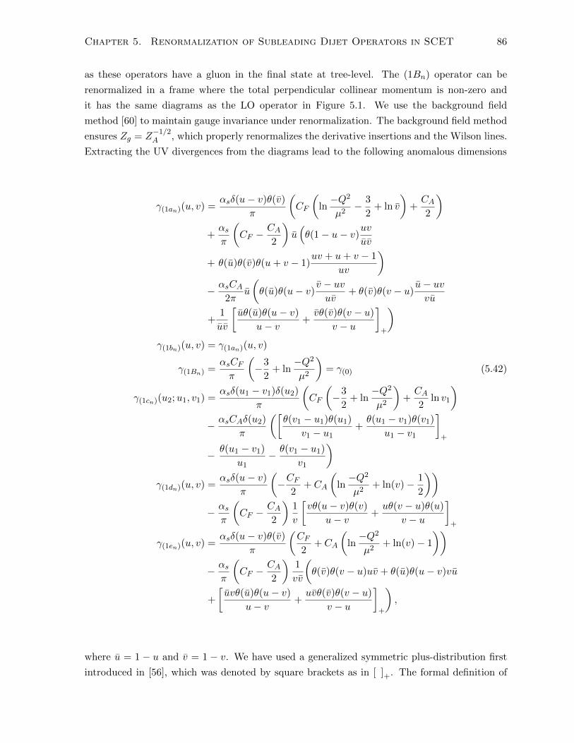
Chapter 5. Renormalization of Subleading Dijet Operators in SCET 86
as these operators have a gluon in the final state at tree-level. The (1Bn) operator can be
renormalized in a frame where the total perpendicular collinear momentum is non-zero and
it has the same diagrams as the LO operator in Figure 5.1. We use the background field
method [60] to maintain gauge invariance under renormalization. The background field method
ensures Zg = Z−1/2A , which properly renormalizes the derivative insertions and the Wilson lines.
Extracting the UV divergences from the diagrams lead to the following anomalous dimensions
γ(1an)(u, v) =αsδ(u− v)θ(v)
π
(CF
(ln−Q2
µ2− 3
2+ ln v
)+CA2
)+αsπ
(CF −
CA2
)u(θ(1− u− v)
uv
uv
+ θ(u)θ(v)θ(u+ v − 1)uv + u+ v − 1
uv
)− αsCA
2πu
(θ(u)θ(u− v)
v − uvuv
+ θ(v)θ(v − u)u− uvvu
+1
uv
[uθ(u)θ(u− v)
u− v+vθ(v)θ(v − u)
v − u
]+
)γ(1bn)(u, v) = γ(1an)(u, v)
γ(1Bn) =αsCFπ
(−3
2+ ln
−Q2
µ2
)= γ(0) (5.42)
γ(1cn)(u2;u1, v1) =αsδ(u1 − v1)δ(u2)
π
(CF
(−3
2+ ln
−Q2
µ2
)+CA2
ln v1
)− αsCAδ(u2)
π
([θ(v1 − u1)θ(u1)
v1 − u1+θ(u1 − v1)θ(v1)
u1 − v1
]+
− θ(u1 − v1)
u1− θ(v1 − u1)
v1
)γ(1dn)(u, v) =
αsδ(u− v)
π
(−CF
2+ CA
(ln−Q2
µ2+ ln(v)− 1
2
))− αs
π
(CF −
CA2
)1
v
[vθ(u− v)θ(v)
u− v+uθ(v − u)θ(u)
v − u
]+
γ(1en)(u, v) =αsδ(u− v)θ(v)
π
(CF2
+ CA
(ln−Q2
µ2+ ln(v)− 1
))− αs
π
(CF −
CA2
)1
vv
(θ(v)θ(v − u)uv + θ(u)θ(u− v)vu
+
[uvθ(u)θ(u− v)
u− v+uvθ(v)θ(v − u)
v − u
]+
),
where u = 1 − u and v = 1 − v. We have used a generalized symmetric plus-distribution first
introduced in [56], which was denoted by square brackets as in [ ]+. The formal definition of
Chapter 5. Renormalization of Subleading Dijet Operators in SCET 87
this distribution is
[θ(u− v)q(u, v) + θ(v − u)q(v, u)]+
≡ − limβ→0
d
du
[θ(u− v − β)
∫ 1+v
udw q(w, v) + θ(v − u− β)
∫ 0
udw q(v, w)
], (5.43)
which is the same as the distribution defined in [56] when u, v ≤ 1. The above definition is also
valid when u, v > 1, which was not required in [56]. Equation (5.42) is our main result.
We can compare the results for γ2(1an) with [56]. The (1an) operator in (5.12) is similar to
the NLO vector heavy-to-light current in [56]. As expected, the anomalous dimension for these
two operators are the same for the non-diagonal terms. They only disagree in the diagonal
terms by the difference of the LO dijet and heavy-to-light operator, which is expected. Also,
the anomalous dimensions of the (1an) and (1bn) operators are the same, as expected from
current conservation in (5.23). We can also check that γ2(1in) = γ2(1in) as expected from CP
invariance. Finally, the (1Bn), (1δ), and (0) operators all have the same anomalous dimension
as expected from RPI.
A final check is to compare the anomalous dimension of the (1en) and (1dn) operators. From
(5.12) we see the (1dn) operator is the limit of the (1en) operator when the quark becomes usoft.
Therefore, we expect in the limit where u ∼ λ2 ∼ v in the (1en) anomalous dimension to recover
the (1dn) anomalous dimension. This is indeed the case as seen in (5.42) ∗∗.
The NLO operators have a cusp in the usoft light-like Wilson lines at xµ = 0. Therefore,
the anomalous dimension depends on at most a single logarithm and can be written in the form
γ2(1i)(µ;u, v) = δ(u− v)ΓC(1i)(αs) ln
−Q2
µ2+ γNC
(1i)(αs;u, v). (5.44)
The coefficient of the logarithm is proportional to the universal cusp anomalous dimension
Γcusp(αs) [61], which means it is possible to perform NLL summation without going to higher
loops. This universal form of (5.44) is confirmed up to O(α2s) corrections in (5.42).
Obviously, solving the RGE analytically is straightforward for the (1Bn) and (1δ) operators
because the anomalous dimension is the same as the LO dijet operator. However, solving the
RGE analytically for the other operators is more difficult. The non-diagonal terms in the (1an)
and (1bn) RGE were solved in [56] by exploiting that the non-diagonal terms in the anomalous
dimensions can be written as f(u, v)S(u, v) where S(u, v) is a symmetric function. For example,
f(u, v) = u for the (1an) operator and 1/(vv) for the (1en) operator. The authors of [56] were
able to expand in an infinite set of Jacobi polynomials with the appropriate weight functions
in order to diagonalize the anomalous dimensions and solve the RGE. We expect that a similar
solution will work for the (1an), (1bn) and (1en) operators. However, the (1cn) and (1dn)
operators are qualitatively different due to the limits on the labels, and a different strategy may
∗∗This limit must be taken carefully, since the u → O(λ2) limit does not commute with the limit in thedefinition of the plus distribution.

Chapter 5. Renormalization of Subleading Dijet Operators in SCET 88
be required. In any case, we believe it may be more practical to solve the RGE numerically,
and we leave this for future work.
5.5 Conclusion
In order to increase the accuracy of the αs(MZ) measurement the O(τ) corrections are becoming
important. Just like for the O(τ0) rate, the O(τ) rate includes large logarithms that must be
summed. We describe how this can be done using SCET and the factorization theorem in [40].
The required operators in the O(τ) factorization theorem must be renormalized so they can be
run from the hard scale to the usoft scale. The running can be done in two stages. First the
NLO and N2LO dijet operators in SCET must be renormalized. These operators are then run
from the hard scale to the intermediate scale. In the next step, the soft operators introduced
in [40] will be renormalized and run from intermediate scale to the usoft scale. This sequence
of running and matching will sum all the large logarithms in the O(τ) rate.
In this chapter, we have started the first step by renormalizing the NLO dijet operators.
Although we have used thrust as a concrete example of an application, our results is applicable
to any observable requiring dijet operators. Because we use the SCET formulation of [26] we
cannot use fermion off-shellness to regulate the IR. Instead we have used a gluon mass, which
leads to individual diagrams being unregulated. However, the sum of all the diagrams from a
given operator is well-defined, as expected. The UV divergences are extracted by looking at the
1/ε poles allowing us to calculate the anomalous dimensions of the NLO operators. We have
checked our results with similar operators for the heavy-to-light currents in [56] and find good
agreement.
We leave renormalizing the N2LO dijets operators and the soft operators to future work.
Although we have calculated the anomalous dimensions of the NLO operators, and investigated
the possibility of solving the RGE analytically, we believe that it may be more practical to solve
it numerically, which we leave for future work.

Chapter 6
The Exclusive kT and C/A Dijet
Rates in SCET with a Rapidity
Regulator
We study the (exclusive) kT and C/A jet algorithms using effective field theory techniques.
Regularizing the virtualities and rapidities of graphs in SCET, we are able to write the next-
to-leading-order dijet cross section as the product of separate hard, jet, and soft contributions.
For the C/A algorithm, we show how to reproduce the Sudakov form factor to next-to-leading
logarithmic accuracy previously calculated by the coherent branching formalism. Our resummed
expression only depends on the renormalization group evolution of the hard function, rather
than on that of the hard and jet functions as is usual in SCET. We comment that regularizing
rapidities in this case is necessary for assessing effects of scale variations, but not for obtaining
the resummed expression. The text in this chapter is reproduced in [62].
6.1 Introduction
Jets are important for understanding the background to new physics being investigated at the
Large Hadron Collider. Jet production is a multiscale process that involves the large energy
of the jet, Q, and its small invariant mass, mjet, given by the details of the jet definition. A
hierarchy of scales Q� mjet gives rise to large logarithms of the form L ≡ ln(Q2/m2jet)� 1 in
perturbative calculations. These logarithms manifest in the jet production rate in the form
R =∞∑n=0
2n∑m=0
RnmαnsL
m, (6.1)
where αs is the strong coupling constant. Even when αs � 1, the large logarithms will ruin
perturbation theory when αsL2 ∼ 1.
Well-known perturbative QCD (pQCD) techniques based on factorization theorems [5] and
89

Chapter 6. The Exclusive kT and C/A Dijet Rates in SCET . . . 90
the coherent branching formalism [3] can sum these logarithms by writing the series (6.1) as
R = C(αs)Σ(αs, L), (6.2)
where
C(αs) =
∞∑n=0
Cnαns , (6.3)
ln Σ(αs, L) = Lf0(αsL) + f1(αsL) + αsf2(αsL) + . . . .
The coefficient function C(αs) contains no large logarithms L, while Σ(αs, L) sums the loga-
rithms. The f0 term sums the leading logarithms (LL), the f1 term sums the next-to-leading
logarithms (NLL), and the fn≥2 terms sum the subleading logarithms. In this chapter we will
always refer to the logarithmic order in the exponent (6.3) as opposed to the logarithmic order
in the perturbative rate (6.1).
An example of a jet definition is the (exclusive) kT jet algorithm [6,63], proposed to resolve
the exponentiation issue of the earlier JADE algorithm [6,64,65]. The kT and JADE algorithms
combine final-state partons into jets using a distance measure yij for all pairs of final-state
partons {i, j}. If the smallest yij is smaller than some pre-determined resolution parameter yc,
then that pair of partons are combined and all the yij ’s are re-calculated. The procedure is
repeated until all yij > yc, and these pseudo-partons are then called jets. The kT algorithm
measure for e+e− → jets is
yij = 2(1− cos θij)min(E2
i , E2j )
Q2(6.4)
where Q is the centre-of-mass energy, θij the angle between the final-state pair, and Ei,j their
respective energy. We are interested in a two-jet final state where the cut parameter is small.
Jets in the yc � 1 region have small mass mjet ≈√ycQ� Q, which gives rise to large logarithms
L ≡ ln(1/yc). The kT dijet production rate has been calculated using the coherent branching
formalism to full LL accuracy in [6, 63] and partial NLL accuracy in [66]. Clustering effects
among multiple gluon emissions generate unsummed logarithms that start at O(α2sL
2) in the
exponent [49] and ruin the NLL summation of [66].
Another jet definition, the C/A algorithm [4] is defined similarly to the kT algorithm but
avoids clustering effects. Two measures are used in this case: vij = 2(1 − cos θij) and the kT
algorithm measure yij in (6.4). Pairs of partons are ordered based on vij , but only the pair
with the smallest vij is combined when their yij < yc. At O(αs), the kT and C/A algorithms
give the same dijet rate at leading order in yc. However, clustering effects do not show up in
the C/A algorithm to ruin the NLL summation [49]. Therefore, the result in [66] gives full NLL
accuracy for the C/A dijet production.
EFT techniques offer another approach to summing the large logarithms. Using EFTs has

Chapter 6. The Exclusive kT and C/A Dijet Rates in SCET . . . 91
the advantage of using the renormalization group (RG) to sum the large logarithms, as well as
providing a systematic approach to power corrections. In [35] the kT dijet rate was calculated
using SCET to next-to-leading order (NLO). SCET [16–20, 26] describes QCD using highly
boosted “collinear” fields and low energy “soft” fields. SCET has previously been successful in
calculating jet shapes [42,67], where it automatically separated the hard scattering interaction
from the highly boosted interactions in the jets and from the soft radiation between them. Such
a separation allows the rate to be written as the convolution of hard, jet (one for each of the
dijets), and soft functions,
R = H × J × J × S, (6.5)
each of which depends on a different scale. These functions are then run individually to a
common scale for logarithm summation. The authors of [35], however, were unable to use
dimensional regularization to regulate the individual NLO collinear and soft graphs of the kT
dijet rate, making it unclear how to write the rate as separate jet and soft functions as in (6.5).
The C/A dijet rate was not discussed in [35], but its NLO calculation faces identical problem
as the kT dijet rate.
Recently [68,69] a new regulator capable of regulating these divergences has been proposed.
This new “rapidity regulator” effectively places a cut on the rapidities of the fields [69], enabling
the rate to be written as separate scheme dependent jet and soft functions. The rapidity
regulator was used to sum logarithms in the jet broadening event shape [42,68,69], which has a
similar issue at NLO to the kT and C/A dijet rates. The introduction of the rapidity regulator
opens up the possibility of the RG running in another scale ν, in analogy to the usual RG
running scale µ of dimensional regularization.
We propose to extend the work of [35] using the new rapidity regulator and investigate how
to write the kT dijet rate as the product of hard, jet, and soft functions as in (6.5). Our work
provides an application of the rapidity regulator to jet algorithms. Our calculation also applies
to the C/A algorithm as the two dijet rates are identical at NLO. As in [6, 63, 66] we assume
a factorization theorem for both the kT and C/A dijet rates, which allows us to interpret the
SCET collinear and soft graphs as the jet and soft functions that are run using the RG. We
can then use the RG to attempt to sum the large logarithms. We find that we reproduce
the coherent branching formalism result for the kT and C/A dijet rates [66], but that neither
approach sums the logarithms generated by the clustering effects for the kT dijet rate [49]. A
similar result was recently found for the inclusive kT algorithm [70]. We expect our result to
sum all the logarithms in the C/A dijet rate as in the coherent branching formalism, since
clustering effects are absent in this case [49].
Reproducing the coherent branching formalism result for the kT and C/A dijet rates using
SCET only requires the running of the hard function to NLL accuracy. The jet and soft
functions act as a single soft function S = J × J × S that reproduces the infrared physics of
QCD and depends only on a single soft scale. For NLL accuracy, defining separate scheme
dependent jet and soft functions using the rapidity regulator is only required to examine the

Chapter 6. The Exclusive kT and C/A Dijet Rates in SCET . . . 92
effects of scale variations, but not for obtaining the resummed expression.
The rest of the chapter proceeds as follows: in Section 6.2 we review the NLO results
and issues of [35], and in Section 6.3 we show how the rapidity regulator solves these issues.
In Section 6.4 we show our final result with NLL summation excluding clustering effects and
compare with the coherent branching formalism result. We discuss the interpretation of our
results and the utility of the rapidity regulator in Section 6.5. Finally we conclude in Section
6.6.
6.2 Review of Previous Work
The kT algorithm was previously studied using SCET in [35]. SCET is the appropriate EFT
to describe QCD with highly boosted massless fields. Collinear fields describe the boosted
particles, and soft fields describe the low-energy particle exchanges. The interactions within
each sector (soft, collinear in each direction) decouple from one another and are described by
a copy of QCD [26]. The interactions between sectors in the full theory are reproduced in the
currents via Wilson lines [17–20,26].
The appropriate SCET operator for dijet production where n and n are respectively the
light-like directions of the jets is [20, 71]
O2 =[ξnWn
] [Y †nΓYn
] [W †nξn
](6.6)
where ξn,n is a two-component n- or n-collinear spinor. The Wilson lines are defined in mo-
mentum space as
Wn =∑perm
[exp
(−gn · P
n ·An)]
Yn =∑perm
[exp
(−gn · P
n ·As)]
, (6.7)
with Wn and Yn defined analogously. Here Pµ is the momentum operator that acts on the gluon
fields. The fields As, An, and An represent soft, n-, and n-collinear gluon fields respectively.
The matching between QCD and SCET is well known [45] and gives the matching coefficient
C2(µ) = 1 +αsCF
2π
(−1
2ln2 µ2
−Q2− 3
2ln
µ2
−Q2− 4 +
π2
12
)+ . . . (6.8)
and MS counterterm
Z2(µ) = 1 +αsCF
2π
(1
ε2+
3
2ε+
1
εln
µ2
−Q2
)+ . . . . (6.9)
The ellipses denote higher orders in αs. The matching coefficient reproduces the ultraviolet

Chapter 6. The Exclusive kT and C/A Dijet Rates in SCET . . . 93
(a) (b)
Figure 6.1: QCD diagrams for real emission. In SCET the gluon can either be soft (pµ3 =
(k+3 , k
−3 ,~k3⊥)), n-collinear (pµ3 = (k+
3 , p−3 , ~p3⊥)) or n-collinear (pµ3 = (p+
3 , k−3 , ~p3⊥)).
(UV) physics of QCD.
The e+e− → γ∗ → dijet rate is calculated in SCET by summing the collinear and soft
diagrams and integrating over the appropriate phase space. Generally the rate is written in the
form1
σ0
dσdijet
dyc= H × (J × J × S) (6.10)
where σ0 = (4πα2/Q2)∑
f e2f is the Born cross section∗. The soft contribution S describes the
interaction of the soft fields, while the hard function H captures the physics of the hard initial
interaction. The hard function is defined to be H = |C2|2. The jet contributions J and J
describe the interactions of the n- and n-collinear fields respectively.
For perturbative calculations, the contributions in (6.10) are individually written as
F (µ) = 1 + F (1)(µ) + F (2)(µ) + . . . (6.11)
where F = H,J, J , S and F (n) is the O(αns ) term. The two QCD diagrams that contribute to
real emission at NLO are shown in Figure 6.1. In SCET, the gluon can either be soft, n-, or
n-collinear, resulting in six graphs that must be summed. We write all momenta in lightcone
coordinates qµ = (n · q, n · q, ~q⊥) ≡ (q+, q−, ~q⊥). We adopt the convention of [35] and use
the symbol k � Q for soft momentum, and p ∼ Q for large momentum. Contributions from
the NLO collinear and soft graphs in dimensional regularization are given by integrating the
corresponding differential cross sections over the relevant phase space PSF [35]
S(1)(µ) =αsCF
2πfε
∫PSS
dk+3 dk
−3
2
(k+3 k−3 )1+ε
J (1)(µ) =αsCF
2πfε
∫PSn
dk+3 dp
−3
(k+3 p−3 )−ε
Qk+3
[p−3Q
(1− ε) + 2Q− p−3p−3
]J
(1)0 (µ) = 2
αsCF2π
fε
∫PS0
dk+3 dk
−3
(k+3 k−3 )1+ε
(6.12)
∗For dijet rates via a Z0, only the Born cross section is modified. This is irrelevant for our calculation.

Chapter 6. The Exclusive kT and C/A Dijet Rates in SCET . . . 94
(a) (b) (c)
Figure 6.2: NLO kT dijet phase space for (a) n-collinear gluon (b) soft gluon and (c) zero-bin.These plots are taken from [35], and the bold arrows indicate that the plots extend to infinity.The C/A dijet phase space is identical.
n-collinear zero-bin soft
min(k+
3
p−3,
k+3 p−3
(Q−p−3 )2
)< yc k+
3 k−3 < ycQ
2 k+3 (k+
3 + k−3 ) < ycQ2
p−3 <√ycQ k−3 <
√ycQ k−3 (k+
3 + k−3 ) < ycQ2
p−3 > Q(1−√yc)
Table 6.1: Phase space constraints for NLO real emission for the kT and C/A algorithms. Theconstraints are plotted in Figure 6.2.
where J is referred to as the naive collinear graph and J0 the zero-bin. The “true” collinear
contribution requires a zero-bin subtraction [22] and is defined as J(µ) = J(µ) − J0(µ). We
have introduced fε ≡ µ2εeεγE/Γ(1− ε) for later convenience. The n-collinear graph is the same
as the n-collinear graph at NLO, J (1)(µ) = J (1)(µ).
The relevant NLO phase space constraints in SCET are found by applying the kT measure
(6.4) to the qqg final state and expanding in k � p,Q. The phase space constraints for the C/A
algorithm are identical to the kT constraints. At leading order in power counting the fermions
must be collinear, and we define nµ to be in the direction of the quark. The constraints for a soft
and n-collinear gluon are shown in Table 6.1 and plotted in Figure 6.2. The constraints for an
n-collinear gluon are the same as those for an n-collinear gluon with “+” and “−” interchanged.
In [35] it was found that the NLO soft graph can be written as
S(1)(µ) = −2αsCFπ
eεγE
εΓ(1− ε)
(µ2
ycQ2
)ε ∫ 1
0dx
(1− x2
2 )−ε
x+ . . . , (6.13)
where the ellipses denote terms that are properly regulated in dimensional regularization. The
integral in (6.13) is not regularized as x→ 0, and this means that interpreting the soft function
as the sum of the soft graphs as in (6.10) is not well defined. However, it was noted in [35] that
Chapter 6. The Exclusive kT and C/A Dijet Rates in SCET . . . 95
the NLO zero-bin can be written as
J(1)0 (µ) = −αsCF
π
eεγE
εΓ(1− ε)
(µ2
ycQ2
)ε ∫ 1
0
dx
x+ . . . ,
where again the ellipses denote terms that are properly regularized. The x → 0 divergence in
this integral is the same as the soft graph. Because J(1)0 (µ) enters into both J(µ) and J(µ)
with a relative minus sign compared to the soft graph, the total rate (1/σ0)(dσdijetkT (C/A)/dyc) is
properly regularized at NLO as expected.
Decomposing the rate as separately regularized jet and soft functions as in (6.10), where
J and S are respectively the collinear and soft graphs, is therefore not possible using pure
dimensional regularization. The issue of separately well-defined functions comes from how
phase space is being divided between the collinear and soft graphs in this scheme. The soft
graph is being integrated over the region k±3 → 0 while keeping k+3 k−3 ≤ ycQ2. This is a highly
boosted region, and is more naturally associated with the jet function than the soft function.
The jet broadening rate has a similar issue in SCET as shown in [42].
As pointed out in [35], the soft graph can be regulated using a different scheme such as a
cut-off regulator. The cut-off regulator removes the contribution of the aforementioned region
from the soft graph and regulates the integral in (6.13). The jet broadening rate can also be
regularized using a cut-off. The cut-off regulator, however, is not very attractive as it is not
gauge invariant, making it hard to run using the RG. It is also unclear how to define it in the
naive collinear calculation.
Another scheme also studied in [35] is to use off-shellness as an infrared regulator, while
using dimensional regularization to regulate the UV. Here, the small quark and anti-quark
off-shellness regulates the integrals in (6.13) and (6.14). However, the resulting collinear and
soft contributions – including the virtual diagrams – are not individually infrared finite, even
though these infrared divergences cancel in the total NLO rate as expected. Therefore it is
again unclear how to interpret these as the jet and soft functions of (6.10).
In the next section we use the recently introduced rapidity regulator [68, 69] to separate
the low energy theory into jet and soft functions associated with the collinear and soft fields
respectively.
6.3 Next-to-Leading-Order calculation
In this section we show how all the divergences in the phase space of the soft graphs are tamed
with the introduction of the rapidity regulator [68,69]. The rapidity regulator was used to solve
the similar issue and sum the logarithms in jet broadening [68, 69]. The regulator acts as an
energy cut-off in a similar way that dimensional regularization acts as a cut-off on the mass
scale of loop momenta [72]. The form is similar to dimensional regularization and also maintains
gauge invariance [69], unlike a cut-off regulator. We will show in this section that using the
Chapter 6. The Exclusive kT and C/A Dijet Rates in SCET . . . 96
rapidity regulator splits the NLO collinear and soft graphs into separately finite pieces. This
allows us to interpret the jet and soft functions as the collinear and soft interactions respectively.
The rapidity regulator modifies the momentum-space definition of the Wilson lines (6.7)
to [68,69]
Wn =∑perm
exp
(−gn · P
[w2 |n · P|−η
ν−ηn ·An
])
Yn =∑perm
exp
(−gn · P
[w|2P3|−η/2
ν−η/2n ·As
]). (6.14)
Here P3 pulls down the component of momentum in the spatial direction of the jet. The new
parameter η acts similarly to ε in dimensional regularization. The parameter w is a bookkeeping
parameter that is set to one at the end [68, 69]. Implementing the rapidity regulator modifies
the NLO collinear and soft graphs to
S(1)(µ, ν) = 2αsCF
2πw2fε
∫PSs
dk+3 dk
−3
(k+3 k−3 )1+ε
∣∣∣∣k+3 − k
−3
ν
∣∣∣∣−η (6.15)
J (1)(µ, ν) =αsCF
2πfε
∫PSn
dk+3 dp
−3
(k+3 p−3 )−ε
Qk+3
[p−3Q
(1− ε) + 2w2Q− p−3
p−3
(p−3ν
)−ν]
J(1)0 (µ, ν) = 2
αsCF2π
w2fε
∫PS0
dk+3 dk
−3
(k+3 k−3 )1+ε
(k−3ν
)−η.
Note that the phase space constraints PSF are not affected. The pure dimensional regularized
functions are recovered in the η → 0 limit.
Calculating the collinear and soft graphs is now straightforward. As has been previously
demonstrated [69], we must expand in η before ε. As we are considering the yc � 1 region, all
terms subleading in yc are also suppressed.
The naive NLO collinear graph is
J (1)(µ, ν) =αsCF
2π
(4w2
(1− π2
12− ln 2
)− 1
2+ ln 2 +
(1
ε− ln
Q2ycµ2
)(w2(2 + ln yc)−
1
2
)).
(6.16)
We leave in w for now and will set it to one at the end. The logarithms cannot be minimized
at any one scale because we have not yet included the zero-bin subtraction. The NLO zero-bin
contribution is
J(1)0 (µ, ν) =
αsCF2π
w2
(− 2
εη+
1
εlnycQ
2
ν2+
2
ηlnycQ
2
µ2− ln
ycQ2
µ2lnycQ
2
ν2
). (6.17)
Subtracting the zero-bin from the naive collinear graph gives the true (bare) collinear contri-

Chapter 6. The Exclusive kT and C/A Dijet Rates in SCET . . . 97
bution
JB(1)(µ, ν) =αsCF
2π
(4w2
(1− π2
12− ln 2
)− 1
2+ ln 2
+
(1
ε− ln
(Q2ycµ2
))(2w2
(1
η+ 1− 1
2lnQ2
ν2
)− 1
2
)). (6.18)
The collinear logarithms can be minimized at µJ =√ycQ and νJ = Q. The n-collinear
contribution J(µ, ν) is exactly the same as J(µ, ν) at this order in αs.
The NLO soft graph can be calculated similarly. The extra η-dependent piece in (6.15)
regulates the divergence of (6.13). The NLO (bare) soft graph is
SB(1)(µ, ν) =αsCF
2πw2
(ln2 ycQ
2
µ2− π2
3+ 2
(1
ε− 2
η+ ln
ycQ2
ν2
)(1
ε− ln
ycQ2
µ2
)), (6.19)
where the logarithms are minimized at the scales µS =√ycQ = νS . Note that the dimensional
regularization scale of the soft graph is equal to that of the collinear graph, µJ = µS .
Putting the collinear and soft graphs together, as well as the matching coefficient (6.8) and
the counterterm (6.9), the kT and C/A relative dijet rate is
1
σ0
dσdijetkT (C/A)
dyc= H(µ)J(µ, ν)J(µ, ν)S(µ, ν) (6.20)
= 1 +αsCF
2π
(− ln2 yc − 3 ln yc +
π2
6− 1− 6 ln 2
)+O(α2
s),
which exactly reproduces the pQCD [6, 65, 66]. All the graphs must be evaluated at the same
(µ, ν). Notice that the ν dependence must cancel between the collinear and soft graphs because
H is ν-independent. This is a general result and means that, when added together, the η
dependence of the J, J and S counterterms must vanish [68].
We find that unlike in [35], we can define the jet and soft functions in (6.10) as the collinear
and soft interactions respectively. In the next section we show how to sum the logarithms using
the RG by running each function individually. We then compare the summed expression to the
coherent branching formalism result.
6.4 Next-to-leading logarithm summation
We wish to calculate both f0 and f1 of (6.3) to sum the logarithms and compare to [66]. Because
we have two UV regulators, the jet and soft functions now run through a two-dimensional (µ, ν)
space.
The renormalized function F is defined in terms of the bare function FB and counterterm
ZF as FB = ZFF . Therefore, the anomalous dimensions in the two directions of the (µ, ν)

Chapter 6. The Exclusive kT and C/A Dijet Rates in SCET . . . 98
space are found using
γµF (µ, ν) = −(
∂
∂ lnµ+ β(αs)
∂
∂αs
)lnZF
γνF (µ, ν) = −(
∂
∂ ln ν+ β(w)
∂
∂w
)lnZF (6.21)
where F = H,J, S. The running of the coupling constant β(αs) = −2αsε+O(α2s) is well-known
and β(w) = −ηw/2 exactly [69]. The counterterms of the jet and soft functions are found from
(6.18) and (6.19) to be
ZS =1 +αsCF
2π
(2
ε2− 4
εη+
2
εlnµ2
ν2+
4
ηlnµ0
2
µ2
)+ . . .
ZJ =1 +αsCF
2π
(2
εη+
3
2ε− 1
εlnQ2
ν2− 2
ηlnµ0
2
µ2
)+ . . . (6.22)
where we have set w = 1, µ02 = ycQ
2, and the ellipses here denote higher orders in αs. The
hard function counterterm Z−1H ≡ |Z2|2 = ZSZ
2J as expected. The NLO anomalous dimensions
are
γµS =2αsCFπ
lnµ2
ν2γµJ =
αsCFπ
(3
2+ ln
ν2
Q2
)γνS =
2αsCFπ
lnµ0
2
µ2γνJ = −αsCF
πlnµ0
2
µ2
γµH ≡ γH = −αsCFπ
(3 + 2 ln
µ2
Q2
). (6.23)
The hard anomalous dimension in the ν direction vanishes identically because Z2 is ν-independent.
For consistency in the running, we must have
− ~γH = 2~γJ + ~γS , (6.24)
where ~γF = (γµF , γνF ) = −~∇ lnZF with ~∇ ≡
(µ ddµ , ν
ddν
). From (6.23), we see that these
conditions are satisfied at NLO.
The anomalous dimensions allow the functions to be run to any scale. However, unlike
in the usual case of only using dimensional regularization to regulate the UV, the hard, jet,
and soft functions are now scalar functions defined over a two-dimensional (µ, ν) space. Path
independence of running is equivalent to the curl of ~γF vanishing. This vanishing curl gives the
condition
µd
dµγνF (µ, ν) = ν
d
dνγµF (µ, ν), (6.25)
which, along with (6.24), must be satisfied to all orders in αs. We show in the Appendix that

Chapter 6. The Exclusive kT and C/A Dijet Rates in SCET . . . 99
the soft ν anomalous dimension can be written as
γνS(µ) = γνS(µ0) +
∫ µ
µ0
dµ′
µ′
(νd
dνγµS(µ′, ν)
), (6.26)
where the general form of the soft µ anomalous dimension is taken to be
γµS(µ, ν) = ΓS [αs(µ)] lnµ2
ν2+ γS [αs(µ)]. (6.27)
Here ΓS is called the cusp anomalous dimension. The γνS(µ0) contains no logarithms and all
the logarithmic dependency of γνS(µ) is determined by the µ anomalous dimension. A similar
expression to (6.26) appears in [69]. The hard anomalous dimension has a similar form as (6.27)
with ν = Q [42]. The jet anomalous dimension is completely constrained by the hard and soft
anomalous dimensions from (6.24).
We can use the above to solve the RG equations and sum the logarithms. Each function
F (µ, ν) must be evolved from the scale that minimizes its logarithms (µF , νF ) to a common
scale. The solution to the RG equations gives the running of each function
F (µ2, ν2) = F (µ1, ν1)e∫ µ2µ1
dµµγµF (µ,ν2)
e∫ ν2ν1
dννγνF (µ1,ν)
(6.28)
where we have chosen to run in ν first but path independence is guaranteed with the use of
(6.26). The summed rate for the path in Figure 6.3 is therefore
1
σ0
dσdijetkT (C/A)
dyc= H(µH)J(µJ , νJ)J(µJ , νJ)S(µS , νS)
× eKH(µH ,µJ )
(µJQ
)ωH(µH ,µJ )(νSνJ
)ωS(µJ ,µ0)
(6.29)
where we have run to a general (µ, ν), and used the consistency equations (6.24) and path
independence (6.26) to write everything in terms of the hard and soft running. Terms subleading
to NLL accuracy have been suppressed. Because of path independence, we can choose any other
path and get the same NLL terms. The summed rate is both µ- and ν-independent, as expected.
The running kernels in (6.29) are defined as
ωF (µ1, µ2) = −Γ0F
β0
[ln r +
(K − β1
β0
)αs(µ2)
4π(r − 1)
]KF (µ1, µ2) = −
γ0F
2β0ln r −
2πΓ0F
β20
[r − 1− r ln r
αs(µ1)(6.30)
+
(K − β1
β0
)1− r + ln r
4π+
β1
8πβ0ln2 r
],
where we denote r = αs(µ1)/αs(µ2). The coefficients ΓnF and γnF are given from the general

Chapter 6. The Exclusive kT and C/A Dijet Rates in SCET . . . 100
µ
Q
µ0
νJ
S
H
νS νJ
µJ
µS
µ
ν
µH
γH
γµJ (νJ)
γµJ (ν)γµ
S(ν)
γµS(νs)
γνS(µ0) γνJ(µ0)
Figure 6.3: Running each function from (µF , νF ) to (µ, ν).
form of the anomalous dimension (6.27) as
ΓF [αs(µ)] =(αs
4π
)Γ0F +
(αs4π
)2Γ1F + . . .
γF [αs(µ)] =(αs
4π
)γ0F +
(αs4π
)2γ1F + . . . (6.31)
where from (6.23) we can read off
Γ0H = −8CF γ0
H = −12CF
Γ0S = 8CF γ0
S = 0. (6.32)
The β-function of the coupling constant αs also has an expansion
β[αs(µ)] = −2αs
[(αs4π
)β0 +
(αs4π
)2β1 + . . .
](6.33)
where
β0 =11CA
3−
2nf3
β1 =34C2
A
3−
10CAnf3
− 2CFnf . (6.34)
The two-loop running in the coupling constant αs(µ) gives
αs(Q)
αs(µ)= 1 +
αs(Q)β0
4πlnµ2
Q2+αs(Q)β1
4πβ0ln
(1 +
αs(Q)β0
4πlnµ2
Q2
). (6.35)
The factor
K ≡(
67
9− π2
3
)CA −
10
9nf (6.36)

Chapter 6. The Exclusive kT and C/A Dijet Rates in SCET . . . 101
0
0.2
0.4
0.6
0.8
1
-4 -3 -2 -1 0 1 2 3 4 5 6 7 8 9
NLONLO/LL
NLO/NLL
NLONLO/LL
NLO/NLL
Figure 6.4: Plots of (6.38) for LL and NLL accuracy. NLO is the order in αs the coefficientfunction C(αs) of (6.3) is taken to. The multipole expansion breaks down before L → 0 oryc → 1, and the inclusion of NLO terms in C(αs) improves accuracy of the curve over thisregion. The procedure for calculating the error bands is described in the text.
is the well-known ratio of the one- and two-loop cusp anomalous dimensions, K = Γ1F /Γ
0F
[42, 66], and is required for the NLL summation.
Choosing the scales that minimize the logarithms in the hard, jet, and soft functions
µH = Q µJ = µS = µ0
νJ = Q νS = µ0 (6.37)
simplifies (6.29) to
1
σ0
dσdijetkT (C/A)
dyc= H(Q)J(µ0, Q)J(µ0, Q)S(µ0, µ0)eKH(Q,µ0)
(µ0
Q
)ωH(Q,µ0)
, (6.38)
which sums the large logarithms to partial NLL accuracy for the kT dijet rate and full NLL
accuracy for the C/A dijet rate. From the above equation we can see that only the RG of the
hard function is required for the summation to NLL accuracy. The action of running in rapidity
cancels between the jet and soft functions. We will elaborate more on this issue in the following
section.
We can now find the functions f0 and f1 of (6.3) from (6.38). The LL summation comes
Chapter 6. The Exclusive kT and C/A Dijet Rates in SCET . . . 102
from setting γ0H = K = β1 = 0. For the C/A dijet rate, the NLL summation comes from the
terms proportional to a single power of γ0H , K, and β1. Therefore,
f0 = −Γ0H
2β0
(1 +
ln(1− x)
x
)(6.39)
f1 =γ0H
2β0ln(1− x) +
Γ0HK
2β20
(x
1− x+ ln(1− x)
)−
Γ0Hβ1
2β30
(x+ ln(1− x)
1− x+
1
2ln2(1− x)
)where x ≡ αsCFβ0L/(4π). Using (6.32) we see that the functions agree exactly with the
coherent branching formalism result [66]. We plot the summed rate in Figure 6.4 as a function
of ln(1/yc). The maximum jet production is at around yc ' 0.2.
The error bars in Figure 6.4 are found by varying the scales µH,J,S and νJ,S in (6.29) by
2 and 1/2 of their values in (6.37). We vary the jet and soft scales together to maintain the
µJ ≈ µS scaling. Varying the νF scales without varying µJ produces no error due to the
exponent ωS(µJ = µ0, µ0) = 0. We take a naive approach to estimate the correlated errors by
varying µJ and νF together, and taking the geometric mean of the resulting percent errors.
6.5 Discussion
That only the RG of the hard function is necessary to reproduce the coherent branching for-
malism result of [66] to NLL accuracy suggests the kT and C/A dijet rate should be written
as
1
σ0
dσdijetkT (C/A)
dyc= H(µ)S(µ). (6.40)
Here the new soft function S(µ) = J(µ)J(µ)S(µ) is the combined collinear and soft graphs and
is well defined at NLO in pure dimensional regularization as seen in [35] and Section 6.2. This
new soft function is also infrared finite, as shown by using off-shellness to regulate the infrared
divergences of the collinear and soft graphs [35]. By running the functions between µH = Q
and µS =√ycQ = µS,J the is reproduced to NLL accuracy for the C/A algorithm.
By choosing to run along the particular path in Figure 6.5, it is clear that only the combined
collinear and soft graphs are required for reproducing the resummed expression (6.38). Along
this path, the general form of the ν anomalous dimension (6.26) becomes
γνS(µ0) = αs(µ0)∑m≥0
γ(m)S αms (µ0), (6.41)
which contains no large logarithms. For NkLL accuracy only the m ≤ k terms are required.
However, in general the γ(0)S term, which is required for NLL accuracy, vanishes as seen in the
kT and C/A dijet rate above and all the cases in [69]. For N2LL accuracy, therefore, only the
hard running and the γ(1)S term are required. However, understanding the dependence on the
scale µ0 requires the rapidity regulator as discussed in [69].

Chapter 6. The Exclusive kT and C/A Dijet Rates in SCET . . . 103
Figure 6.5: Running the functions along a particular path. Note that, up to NLL accuracy, thesummed result is independent of the path chosen and the final (µ, ν) point.
6.6 Conclusion
We have studied the (exclusive) kT and C/A dijet rates using effective theory methods, and
shown how to reproduce the coherent branching formalism result to NLL accuracy. We must
use the rapidity regulator if we wish to separate the NLO rate into regularized jet and soft
functions. We have demonstrated how to sum logarithms to LL and NLL accuracy using the
rapidity regulator in a path independent way, which can be generalized to any process that has
a factorization theorem. We comment that the rapidity regulator is necessary for evaluating
effects of scale variations, but not for summing the large logarithms to NLL accuracy in the
example of the C/A dijet rate. The same resummed result can be achieved if we consider the
combined jet and soft function and run to the common jet and soft scale. We also find that
using SCET with a rapidity regulator does not account for clustering effects and cannot improve
the coherent branching formalism result for the kT dijet rate. A more complicated SCET-like
theory may be able to properly account for these clustering effects, however, we do not explore
such a theory in this thesis.
6.7 Appendix: General Rapidity Anomalous Dimension
Here we show, using the soft function as an example, how to obtain (6.26), which allows us to
sum to NLL accuracy. Our argument relies on factorization of scales, the consistency condition
(6.24), the vanishing curl (6.25), the general form of γH , and that the anomalous dimensions
are defined perturbatively in αs.
Factorization means that the anomalous dimensions of each function are sensitive only to
scales relevant to it. Therefore, the ν dependence of ~γJ and ~γS will only be of the form ln(ν/Q)
and ln(ν/µ0) respectively. The consistency condition (6.24) requires that all ν dependence of
~γJ and ~γS must cancel to all orders in perturbation theory. As γµH is cusp-like and γνH vanishes,

Chapter 6. The Exclusive kT and C/A Dijet Rates in SCET . . . 104
Figure 6.6: Running the soft function in a rectangular path back to itself. Naively this resultsin a LL phase when ν2 � ν1.
γµF can have at most a linear dependence on ln(ν/νF ) and γνF must have no ν dependence.
The appearance of ln(µ/µ0) in ~γF , on the other hand, is not constrained. These logarithms
can show up in arbitrary powers, as long as they cancel one another in the sum ~γS + 2~γJ to
reproduce ~γH . Fortunately these logarithms have negligible effect on NLL summation. This
fact is made clear by the particular path shown in Figure 6.5, where these logarithms vanish in
γνS(µ0). Because of this and path independence, we suppress these terms in (6.27).
The fact that γνS is independent of ν to all orders in αs is also fixed by the form of γµS in
(6.27) and the vanishing curl (6.25). Taking this general form and applying ν(d/dν) to both
sides of (6.25) yields
µd
dµ
(νd
dνγνS(µ, ν)
)= 0. (6.42)
This means that ν(d/dν)γνS(µ, ν) is independent of µ and in particular αs(µ). Such terms do
not exist in perturbation theory, unless γνS(µ, ν) is independent of ν.
The full µ dependence of γνS can therefore be obtained from γµS via integrating (6.25):
γνS(µ) = γνS(µ′) +
∫ µ
µ′
dµ′′
µ′′
(νd
dνγµS(µ′′, ν)
). (6.43)
In (6.26) we choose µ′ = µ0 such that all logarithms in γνS(µ′) vanish and only the non-
logarithmic terms remain. If (6.43) is not used, then running the soft function in the closed
path shown in Figure 6.6 would result in a large phase that spoils the LL accuracy of the results
when ν2 � ν1.

Chapter 7
Conclusion
Testing large energy QCD requires understanding how jets are produced. We have discussed
the difficulties in calculating jet rates for large energy collisions. Jets are important to be able
to analyze properly because they provide good tests of QCD as well as a large background
to events at colliders. On the theoretical side, jet rates are interesting to calculate because
they involve multiple scales that are usually correlated. Separating the physics at each of these
scales is challenging. We have explored how to use Effective Field Theory (EFT) techniques to
separate these scales and improve theoretical results by calculating the subleading order effects.
While we are only interested in the perturbative rate where the QCD coupling constant
is small, the hierarchy of scales in jet rates leads to large logarithmic enhancements in the
perturbative rate. We have discussed how EFTs provide a framework for separating the physics
at each of these scales and systematically improving calculations. The appropriate EFT for jet
physics is soft-collinear effective theory (SCET). We introduced two formulations of SCET: the
first where the large energy of the jet is removed from the theory leaving behind two-component
spinors that couple to Wilson lines. The second formulation did not remove the large energy and
instead described the theory as QCD fields coupled to Wilson lines. While both formulations
are equivalent, the second formulation, discussed in Chapter 3, explicitly separates the various
sectors at each order in the small jet mass over large energy expansion.
Thrust is a jet shape that can be used to make accurate measurements of αs(MZ). The rate
had previously been factorized at leading order in the thrust parameter and the logarithmic
enhancements had been summed to a high degree. We showed in Chapter 4 how using the
explicit separation of collinear and soft fields in the formulation of SCET in Chapter 3, a
factorization theorem could be derived at subleading orders. This factorization was the first
ever factorization of a jet rate at subleading orders.
The subleading rate also has enhancements from large logarithms that ruins the perturbative
expansion in the QCD coupling constant αs(Q) � 1. These logarithms can be summed by
solving the Renormalization Group Equations (RGE) for the operators set out in Chapter 4. In
Chapter 5 we started to renormalize the next-to-leading order operators in Chapter 3. We found
that this was most easily done with a gluon mass regulator that leads to divergent integrals
105

Chapter 7. Conclusion 106
from each sector, but are convergent in the sum of all diagrams.
Finally, we discussed the kT and C/A jet algorithms in the context of SCET. Unlike the
thrust observable, the kT and C/A two-jet rates depend only on two invariant scales. This
leads to the soft and collinear graphs being individually divergent despite expecting them to
separate at O(αs). A rapidity regulator is introduced that properly regulates the divergences
appearing in these graphs. This allows the individual graphs to be calculated separately. We
show how the general form of the anomalous dimensions of the soft and jet operators at all
orders in αs. The general form can be written in such a way that leading-logarithmic accuracy
does not require the introduction of any new regulators. The leading-logarithmic result can
instead be obtained by running only the hard function, which is the square of the SCET Wilson
coefficient. The rapidity regulator is only required for determining how the rate depends on the
renormalization scales.
7.1 Future Directions
We showed using the SCET formulation in Chapter 3 that the soft and collinear fields decoupled
to all orders in power counting when matching from QCD at the ultraviolet (UV) scale Q.
However, we are uncertain why it was necessary to introduce the soft fields at the UV scale
in the first place in order to properly reproduce the infrared (IR) of QCD. As was discussed
in Chapter 2, knowledge of the existence of multiple IR scales is not required for matching
at the UV scale. These scales are only necessary after running the EFT theory down to the
next IR scale. In SCET, the soft fields are typically at a scale well below the collinear fields
as seen in (2.18) and (2.19). In fact, soft fields can be described as a subset of collinear fields
in this momentum scaling. However, the inclusion of soft fields at Q is currently necessary for
reproducing the IR of QCD in all formulations of SCET, which is counterintuitive. A future
direction would be to expand the work of Chapter 3 so soft fields are only introduced at a lower
IR scale.
The necessity for the introduction of a new regulator in the perturbative calculation for jet
rates involving only two scales, such as in Chapter 6, is also unexpected. The new regulator
appears to be required to maintain the scale independence of the rate. The resulting rapidity
logarithm appears to be an artifact of matching onto SCET when there are only two scales
instead of the usual three scales in rates such as thrust. When there are only two scales, the
UV scale and an IR soft scale, the soft and collinear fields both become heavy at the same soft
scale and must be removed from our description. SCET is then matched onto a new effective
theory. When there are three scales, the soft and collinear fields become heavy and are removed
at two widely separated scales. The rapidity logarithm may be due to a matching condition at
the lowest soft scale that is not typically necessary for calculations involving three scales, such
as thrust.
Finally, the work in Chapters 4 and 5 make it possible to increase the precision of the mea-

Chapter 7. Conclusion 107
surement of αs(MZ). Currently, the SCET calculation of thrust has given the most accurate
measurement of the strong coupling constant [50]. However, the value differs from what is ex-
pected from other measurement techniques, such as Lattice QCD. The SCET analysis included
the subleading rate in the thrust parameter and convoluted this subleading rate with the non-
perturbative soft function. Including, not only the summed logarithms in the subleading rate,
but also properly convoluting the non-perturbative soft function with the SCET soft operator
could give a more precise measurement of αs(MZ).

Bibliography
[1] Georges Aad et al. Measurement of the Higgs boson mass from the H → γγ and H →ZZ∗ → 4` channels with the ATLAS detector using 25 fb−1 of pp collision data. Phys.Rev.,
D90:052004, 2014.
[2] Vardan Khachatryan et al. Precise determination of the mass of the Higgs boson and
tests of compatibility of its couplings with the standard model predictions using proton
collisions at 7 and 8 TeV. 2014.
[3] S. Catani, L. Trentadue, G. Turnock, and B.R. Webber. Resummation of large logarithms
in e+ e- event shape distributions. Nucl.Phys., B407:3–42, 1993.
[4] Yuri L. Dokshitzer, G.D. Leder, S. Moretti, and B.R. Webber. Better jet clustering algo-
rithms. JHEP, 9708:001, 1997.
[5] John C. Collins, Davison E. Soper, and George F. Sterman. Factorization of Hard Processes
in QCD. Adv.Ser.Direct.High Energy Phys., 5:1–91, 1988. publ. in ‘Perturbative QCD’
(A.H. Mueller, ed.) (World Scientific Publ., 1989).
[6] Stefano Catani. Jet topology and new jet counting algorithms. Erice Proceedings, ‘QCD
at 200-TeV’, 21-41, 1991.
[7] George F. Sterman. Partons, factorization and resummation, TASI 95. 1995.
[8] Matteo Cacciari, Gavin P. Salam, and Gregory Soyez. The Anti-k(t) jet clustering algo-
rithm. JHEP, 0804:063, 2008.
[9] Edward Farhi. A QCD Test for Jets. Phys.Rev.Lett., 39:1587–1588, 1977.
[10] John E. Huth, Naor Wainer, Karlheinz Meier, Nicholas Hadley, F. Aversa, et al. Toward
a standardization of jet definitions. 1990.
[11] Joseph Polchinski. Effective field theory and the Fermi surface. 1992.
[12] M. Luke. Bottom quark physics and the heavy quark expansion. pages 193–242, 2002.
[13] Siegfried Bethke. World Summary of αs (2012). Nucl.Phys.Proc.Suppl., 234:229–234, 2013.
108
Bibliography 109
[14] Aneesh V. Manohar and Mark B. Wise. Heavy quark physics. Camb. Monogr. Part. Phys.
Nucl. Phys. Cosmol., 10:1–191, 2000.
[15] Michael E. Luke and Aneesh V. Manohar. Reparametrization invariance constraints on
heavy particle effective field theories. Phys.Lett., B286:348–354, 1992.
[16] Christian W. Bauer, Sean Fleming, and Michael E. Luke. Summing Sudakov logarithms
in B → Xsγ in effective field theory. Phys. Rev., D63:014006, 2000.
[17] Christian W. Bauer, Sean Fleming, Dan Pirjol, and Iain W. Stewart. An effective theory
for collinear and soft gluons: heavy to light decays. Phys. Rev., D63:114020, 2001.
[18] Christian W. Bauer and Iain W. Stewart. Invariant operators in collinear effective theory.
Phys. Lett., B516:134–142, 2001.
[19] Christian W. Bauer, Dan Pirjol, and Iain W. Stewart. Soft collinear factorization in
effective field theory. Phys. Rev., D65:054022, 2002.
[20] Christian W. Bauer, Sean Fleming, Dan Pirjol, Ira Z. Rothstein, and Iain W. Stewart.
Hard scattering factorization from effective field theory. Phys. Rev., D66:014017, 2002.
[21] M. Beneke, A.P. Chapovsky, M. Diehl, and T. Feldmann. Soft collinear effective theory
and heavy to light currents beyond leading power. Nucl. Phys., B643:431–476, 2002.
[22] Aneesh V. Manohar and Iain W. Stewart. The zero-bin and mode factorization in Quantum
Field Theory. Phys. Rev., D76:074002, 2007.
[23] Keith S.M. Lee and Iain W. Stewart. Factorization for power corrections to B → Xsγ and
B → Xu`ν. Nucl. Phys., B721:325–406, 2005.
[24] M. Beneke and T. Feldmann. Multipole expanded soft collinear effective theory with non-
Abelian gauge symmetry. Phys. Lett., B553:267–276, 2003.
[25] M. Beneke, F. Campanario, T. Mannel, and B.D. Pecjak. Power corrections to B →Xu`ν(Xsγ) decay spectra in the ‘shape-function’ region. JHEP, 0506:071, 2005.
[26] Simon M. Freedman and Michael Luke. SCET, QCD and Wilson Lines. Phys.Rev.,
D85:014003, 2012.
[27] A. Bassetto, M. Dalbosco, I. Lazzizzera, and R. Soldati. Yang-Mills theories in the light
cone gauge. Phys. Rev., D31:2012, 1985.
[28] Thomas Becher, Matthias Neubert, and Ben D. Pecjak. Factorization and momentum-
space resummation in deep-inelastic scattering. JHEP, 0701:076, 2007.
[29] Christian W. Bauer, Oscar Cata, and Grigory Ovanesyan. On different ways to quantize
Soft-Collinear Effective Theory. 2008.

Bibliography 110
[30] R.Keith Ellis, W. Furmanski, and R. Petronzio. Unraveling higher twists. Nucl. Phys.,
B212:29, 1983.
[31] Christian W. Bauer, Michael E. Luke, and Thomas Mannel. Light cone distribution func-
tions for B decays at subleading order in 1/mb. Phys. Rev., D68:094001, 2003.
[32] Dan Pirjol and Iain W. Stewart. A Complete basis for power suppressed collinear ultrasoft
operators. Phys.Rev., D67:094005, 2003.
[33] Christian W. Bauer, Dan Pirjol, and Iain W. Stewart. On power suppressed operators and
gauge invariance in SCET. Phys. Rev., D68:034021, 2003.
[34] Junegone Chay and Chul Kim. Collinear effective theory at subleading order and its
application to heavy - light currents. Phys. Rev., D65:114016, 2002.
[35] William Man-Yin Cheung, Michael Luke, and Saba Zuberi. Phase space and jet definitions
in SCET. Phys. Rev., D80:114021, 2009.
[36] Stephen D. Ellis, Christopher K. Vermilion, Jonathan R. Walsh, Andrew Hornig, and
Christopher Lee. Jet shapes and jet algorithms in SCET. JHEP, 1011:101, 2010.
[37] Ahmad Idilbi and Ignazio Scimemi. Singular and regular gauges in Soft Collinear Effective
Theory: the introduction of the new Wilson line T. Phys. Lett., B695:463–468, 2011.
[38] Miguel Garcia-Echevarria, Ahmad Idilbi, and Ignazio Scimemi. SCET, Light-Cone Gauge
and the T-Wilson Lines. Phys.Rev., D84:011502, 2011.
[39] Stefan W. Bosch, Matthias Neubert, and Gil Paz. Subleading shape functions in inclusive
B decays. JHEP, 0411:073, 2004.
[40] Simon M. Freedman. Subleading Corrections To Thrust Using Effective Field Theory.
2013.
[41] Christian W. Bauer, Sean P. Fleming, Christopher Lee, and George F. Sterman. Factor-
ization of e+e- Event Shape Distributions with Hadronic Final States in Soft Collinear
Effective Theory. Phys.Rev., D78:034027, 2008.
[42] Andrew Hornig, Christopher Lee, and Grigory Ovanesyan. Effective Predictions of Event
Shapes: Factorized, Resummed, and Gapped Angularity Distributions. JHEP, 05:122,
2009.
[43] Vicent Mateu, Iain W. Stewart, and Jesse Thaler. Power Corrections to Event Shapes with
Mass-Dependent Operators. 2012.
[44] G. Kramer and B. Lampe. Jet Cross-Sections in e+e− Annihilation. Fortsch.Phys., 37:161,
1989.

Bibliography 111
[45] Aneesh V. Manohar. Deep inelastic scattering as x→ 1 using soft collinear effective theory.
Phys.Rev., D68:114019, 2003.
[46] Christian W. Bauer, Dan Pirjol, and Iain W. Stewart. Power counting in the soft collinear
effective theory. Phys.Rev., D66:054005, 2002.
[47] Christian W. Bauer, Andrew Hornig, and Frank J. Tackmann. Factorization for generic
jet production. Phys.Rev., D79:114013, 2009.
[48] Simon M. Freedman and Raymond Goerke. Renormalization of Subleading Dijet Operators
in Soft-Collinear Effective Theory. 2014.
[49] A. Banfi, G.P. Salam, and G. Zanderighi. Semi-numerical resummation of event shapes.
JHEP, 0201:018, 2002.
[50] Riccardo Abbate, Michael Fickinger, Andre H. Hoang, Vicent Mateu, and Iain W. Stewart.
Thrust at N3LL with Power Corrections and a Precision Global Fit for αs(mZ). Phys.Rev.,
D83:074021, 2011.
[51] Thomas Becher and Matthew D. Schwartz. A precise determination of αs from LEP thrust
data using effective field theory. JHEP, 0807:034, 2008.
[52] Jui-yu Chiu, Andreas Fuhrer, Andre H. Hoang, Randall Kelley, and Aneesh V. Manohar.
Soft-Collinear Factorization and Zero-Bin Subtractions. Phys.Rev., D79:053007, 2009.
[53] Ilya Feige and Matthew D. Schwartz. An on-shell approach to factorization. Phys.Rev.,
D88(6):065021, 2013.
[54] Ilya Feige and Matthew D. Schwartz. Hard-Soft-Collinear Factorization to All Orders.
2014.
[55] Christian W. Bauer, Christopher Lee, Aneesh V. Manohar, and Mark B. Wise. Enhanced
nonperturbative effects in z decays to hadrons. Phys. Rev. D, 70:034014, Aug 2004.
[56] R.J. Hill, T. Becher, Seung J. Lee, and M. Neubert. Sudakov resummation for subleading
SCET currents and heavy-to-light form-factors. JHEP, 0407:081, 2004.
[57] Claudio Marcantonini and Iain W. Stewart. Reparameterization Invariant Collinear Op-
erators. Phys.Rev., D79:065028, 2009.
[58] Aneesh V. Manohar, Thomas Mehen, Dan Pirjol, and Iain W. Stewart. Reparameterization
invariance for collinear operators. Phys.Lett., B539:59–66, 2002.
[59] Aneesh V. Manohar and Iain W. Stewart. The zero-bin and mode factorization in Quantum
Field Theory. Phys. Rev., D76:074002, 2007.

Bibliography 112
[60] L.F. Abbott. The Background Field Method Beyond One Loop. Nucl.Phys., B185:189,
1981.
[61] G.P. Korchemsky and A.V. Radyushkin. Renormalization of the Wilson Loops Beyond
the Leading Order. Nucl.Phys., B283:342–364, 1987.
[62] William Man-Yin Cheung and Simon M. Freedman. The Exclusive kT Dijet Rate in SCET
with a Rapidity Regulator. 2012.
[63] S. Catani, Yuri L. Dokshitzer, M. Olsson, G. Turnock, and B.R. Webber. New clustering
algorithm for multi - jet cross-sections in e+ e- annihilation. Phys.Lett., B269:432–438,
1991.
[64] N. Brown and W.James Stirling. Jet cross-sections at leading double logarithm in e+ e-
annihilation. Phys.Lett., B252:657–662, 1990.
[65] N. Brown and W.James Stirling. Finding jets and summing soft gluons: A New algorithm.
Z.Phys., C53:629–636, 1992.
[66] Gunther Dissertori and Michael Schmelling. An Improved theoretical prediction for the
two jet rate in e+ e- annihilation. Phys.Lett., B361:167–178, 1995.
[67] Stephen D. Ellis, Christopher K. Vermilion, Jonathan R. Walsh, Andrew Hornig, and
Christopher Lee. Jet shapes and jet algorithms in SCET. JHEP, 1011:101, 2010.
[68] Jui-yu Chiu, Ambar Jain, Duff Neill, and Ira Z. Rothstein. The Rapidity Renormalization
Group. 2011.
[69] Jui-yu Chiu, Ambar Jain, Duff Neill, and Ira Z. Rothstein. A Formalism for the Systematic
Treatment of Rapidity Logarithms in Quantum Field Theory. 2012.
[70] Randall Kelley, Jonathan R. Walsh, and Saba Zuberi. Abelian Non-Global Logarithms
from Soft Gluon Clustering. 2012.
[71] Christian W. Bauer and Matthew D. Schwartz. Event Generation from Effective Field
Theory. Phys.Rev., D76:074004, 2007.
[72] H. Georgi. Effective field theory. Ann.Rev.Nucl.Part.Sci., 43:209–252, 1993.


![Michael J. Freedman - Stanford Universitymfreed/app/freedman-app-all.pdf · [8] Yevgeniy Dodis, Michael J. Freedman, Stanislaw Jarecki, and Shabsi Walfish. Versatile padding schemes](https://img.pdfslide.net/doc/110x75/5e236cc7a6b48e33f5088c8b/michael-j-freedman-stanford-mfreedappfreedman-app-allpdf-8-yevgeniy-dodis.jpg)