Embed Size (px)
Citation preview

STRUCTURE-PRESERVING ISOGEOMETRICANALYSIS FOR COMPUTATIONAL FLUID DYNAMICS
BY STEVIE-RAY JANSSEN
M.SC. THESISNovember 7th, 2016


STRUCTURE-PRESERVING ISOGEOMETRICANALYSIS FOR COMPUTATIONAL FLUID DYNAMICS
M.SC. THESIS
To obtain the degree Master of Science at Delft University of Technology,
by
Stevie-Ray JANSSEN
Student of Aerospace Engineering and Applied Mathematics,Delft University of Technology,
Delft, The Netherlands.

Thesis Committee:
Aerospace Engineering:Dr. ir. M.I. Gerritsma TU Delft, supervisorProf. dr. S. Hickel TU DelftDr. ir. A. Palha TU Eindehoven
Applied Mathematics:Dr. M. Möller, TU Delft, supervisorProf. dr. ir. C. Vuik TU DelftProf. dr. J.M.A.M. van Neerven TU Delft
November 7th, 2016
An electronic version of this dissertation is available athttp://repository.tudelft.nl/.

CONTENTS
Preface vii
1 Introduction 1
2 Exterior Calculus 52.1 Manifolds and Coordinate Spaces. . . . . . . . . . . . . . . . . . . . . . 62.2 Forms and Operations . . . . . . . . . . . . . . . . . . . . . . . . . . . 102.3 Chains and Cochains . . . . . . . . . . . . . . . . . . . . . . . . . . . . 142.4 The Codifferential and the Inner Product . . . . . . . . . . . . . . . . . . 212.5 Poisson Problems . . . . . . . . . . . . . . . . . . . . . . . . . . . . . . 242.6 Summary of Results . . . . . . . . . . . . . . . . . . . . . . . . . . . . . 26
3 Structure Preserving Isogeometric Analysis 293.1 The Sobolev-DeRham Complex . . . . . . . . . . . . . . . . . . . . . . . 303.2 Basis Functions and Isogeometric Analysis . . . . . . . . . . . . . . . . . 343.3 DeRham Conforming Spline Spaces. . . . . . . . . . . . . . . . . . . . . 403.4 Discretisation of the Poisson Problems . . . . . . . . . . . . . . . . . . . 453.5 Summary of Results . . . . . . . . . . . . . . . . . . . . . . . . . . . . . 48
4 Scalar Transport 514.1 The Interior Product and the Lie Derivative . . . . . . . . . . . . . . . . . 514.2 Transport Problems . . . . . . . . . . . . . . . . . . . . . . . . . . . . . 564.3 Discretisation of Transport Problems . . . . . . . . . . . . . . . . . . . . 614.4 Summary of Results . . . . . . . . . . . . . . . . . . . . . . . . . . . . . 70
5 Euler Equations 715.1 The Euler Equations . . . . . . . . . . . . . . . . . . . . . . . . . . . . 715.2 Discretisation of the Euler equations . . . . . . . . . . . . . . . . . . . . 745.3 Results, and Analysis . . . . . . . . . . . . . . . . . . . . . . . . . . . . 775.4 Summary of Results . . . . . . . . . . . . . . . . . . . . . . . . . . . . . 83
6 Conclusion & Future Directions 85
A DeRham Cohomology 87
B Derivation of Adjoint Relations 90
C Generalised Piola Transformations 93
D Well-Posedness of the Poisson Problem 95
E Derivation of Edge Functions 100
F Construction of Bounded Cochain Projections 102
v

vi CONTENTS
G Derivation of Transport Problems 105
H Construction of Periodic Basis 110
I Derivation of the Euler Equations and Invariants 113
J Proof Discrete Euler Equations Satisfy Conservation Laws 117
K Picard and Newton Linearisation 121
Bibliography 125
Index 128

PREFACE
Man, I went through this thesis project like a loose cannon. I finally found myself nearthe battlefront of knowledge! I was excited to learn, to develop new ideas, and I wanted todo everything. Call it a young man’s hubris. I’ve looked at space-time discretisations, thevariational multiscale method, discontinuous Galerkin, Lagrangian and Eulerian mesh-ing techniques, symplectic time integrators, and, of course, isogeometric analysis andstructure-preserving discretisation techniques. Unsurprisingly, I struggled somewhatwith combining this all into one thesis, which resulted in the fact that some materialhas been removed or moved to appendices to improve both consistency and readability.I encourage any reader to check the appendices as well.
In 2013 I attended dr. Gerritsma’s course on structure-preserving discretisations forCFD. The mathematics fascinated me even though I barely understood what he was talk-ing about (pseudo-differential form-coboundary-operator-mumbo-jumbo). I wanted tolearn more about this stuff, and asked him if I could do my thesis project with him. He,being a nice man and all, accepted my request. He brought me into contact with dr.Möller, who was organising biweekly seminars on isogeometric analysis at that time.Since this stuff was also pretty interesting, I ended up combining both topics into structure-preserving isogeometric analysis for CFD.
I would like to thank them both for guiding me along the way. I would like to thanksome of my predecessors, Hiemstra, dr. Kreeft, Natale, dr. Palha, Rebelo, Toshniwal,old students of dr. Gerritsma, whose theses inspired me and helped me mastering thematerial. I’d like to thank prof. Hughes for having me over at ICES in Austin for a fewmonths. Thank you for your great lectures on isogeometric analysis. Special thanks toRené and Deepesh for your guidance and friendship. I really enjoyed working with youguys. I’d also like to thank the other guys at ICES for letting me kick their asses at fußbal.Finally, I’d like to thank my girlfriend, Mariel, who has taken such good care of me.
Stevie-Ray JanssenRotterdam, November 2016
vii


1INTRODUCTION
Computational Fluid Dynamics (CFD), the field of computer simulations of fluid flows,has established itself as one of the pillars of modern fluid flow research. The field has awide range of theoretical applications which include the research of turbulence, tidal dy-namics, and blood flows, but also knows important industry applications as the designof aircraft, micro-processors, or submarines. The Navier-Stokes equations govern manyfluid flows. The underlying geometric structure of these equations facilitates structuresand symmetries. Classical solution methods often neglect these structures. As a re-sult, these methods fail to conserve invariant quantities, and are unable to simulate thedesired physical behaviour, [1]. Recently it is shown that solution techniques can beconstructed that do preserve the underlying geometry of physics. These techniques areknown as structure-preserving techniques.
"In discretising the incompressible Navier-Stokes’ one encounters two difficulties,p.265 [2]". The first difficulty is the discretisation of the non-linear convective term. Thesecond difficulty used to be the treatment of the saddle-point problem that describesthe relation between pressure and velocity. Structure-preserving methods have reducedthe second difficulty to a triviality. These methods aim at preserving fundamental struc-tures of operators and operands found in partial differential equations (PDE’s). Conceptsfrom differential geometry and algebraic topology are used to analyse these structures.In this approach we distinguish between relations that depend on metric and those thatare purely topological. The topological relations can be described using algebraic equa-tions, which allows exact representation in the discrete setting as argued by Tonti [1].Satisfying these topological relations lies at the heart of structure-preserving discretisa-tion techniques.
The application of differential geometry and algebraic topology has resulted in thedevelopment of a wide variety of structure-preserving discretisation techniques. Roughlyspeaking, they can be split in two groups, each having a different approach of discretisingthe Hodge-? operator. In the first approach one defines an explicit primal- and dual-gridon which the action of the Hodge-? operator is approximated. This approach leads moreto a finite-differencing, or finite-volume type methods. Fundamental works include the
1

1
2 1. INTRODUCTION
work on mimetic finite difference by Hyman, [3], and the work on discrete exterior cal-culus by Desbrun et al., [4]. In another approach one uses the inner product definitionof the Hodge-? operator in a variational approach, leading to finite-element type meth-ods. Fundamental works in are the ones on finite element exterior calculus by Arnoldet al., [5], conforming mimetic discretisations by Bochev and Hyman, [6], and mimeticspectral element method Gerritsma et al, [7].
Isogeometric analysis (IGA) was pitched by Hughes et al. in 2005 to bridge the gapbetween CAD design and analysis, [8]. In this approach Non-Uniform Rational B-splines(NURBS) are used for both representation of the physical geometry and variational anal-sysis. It was shown that NURBS posses superior approximation behaviour in analysisover Lagrange polynomials, classically used in finite elements analysis, [9, 10]. Buffa etal. developed a theoretical framework of structure-preserving isogeometric analaysis forelliptic PDE problems, [11]. Variety of successful implementations include the Maxwellequations by Buffa, [12], and the unsteady Navier-Stokes’ equations by Evans, [13]. Theseworks deal with similar discretisation challenges, e.g. unsteadiness, non-linearity andasymmetric operators, that are also present in the proposed model problem.
The incompressible Euler equations have a rich geometric structure as describedin [14]. The Hamiltonian structure of these was unveiled in the classical work by V.Arnold [15]. An interesting discretisation was introduced by L. Rebholz in which velocityand vorticity are treated as independent variables [16]. The structure-preserving dis-cretisation by Palha makes use of this idea [17]. The study proposed will contribute tothese developments, and will aim at the further development and analysis of structure-preserving techniques for the Euler equations. The main challenge is to discretise thenon-linear convective operator in a structure-preserving manner, i.e. preserving globalquantities as kinetic-energy, vorticity, and enstrophy.
This thesis is the result of a research project on discretisation techniques for CFD.This thesis was written to obtain the degree of Master of Science at the faculties of AerospaceEngineering (AE) and Applied Mathematics (AM) at Delft University of Technology. Theproject was divided in three objectives. The first objective was to study the existing ex-isting structure-preserving IGA framework for elliptic PDE’s, (chapter 2 and chapter 3).The objective for AM was to expand this theoretical framework to discretise hyperbolicPDE’s (chapter 4). The objective for AE was to construct a structure-preserving IGA dis-cretisation for the incompressible Euler equations, chapter 5. All results are combinedin this single thesis document.
In line with the mentioned works we will analyse the PDE’s using concepts from dif-ferential geometry, exterior calculus, and algebraic topology. Fundamental concepts andtheorems from these fields will be introduced and reviewed in chapter 2. We will identifythe DeRham complex, which can also be constructed in a discrete setting, and formulateelliptic PDE problems. In chapter 3 we will introduce a variational framework, the foun-dation of the finite-elements method, introduce concepts from isogeometric analysis,and construct a framework of structure-preserving isogeometric analysis, using the con-cepts introduced in chapter 2. We will use these results to discretise various formulationsof the scalar Poisson problem. In chapter 4 we expand our exterior calculus toolbox, andintroduce variational formulations for hyperbolic PDE’s. We study the scalar transportequation, and discuss various discretisation strategies. Finally, in chapter 5 we introduce

1
3
the Euler equations for incompressible fluids, and derive structure-preserving discreti-sations that conserve integral invariants over time. Conclusions and future directionswill be discussed in chapter 6


2EXTERIOR CALCULUS
The laws of physics are generally analysed using the language of vector calculus. Fol-lowing the works mentioned in the introduction, we will analyse physical relations usingdifferential geometry, exterior calculus, and algebraic topology. The first advantage ofthis approach is that analysis is performed on arbitrary geometries, which are knownas manifolds. Results that will be introduced do not depend on some local descriptionof physics. The second and main advantage of this approach, is that it enables a cleardistinction between relations that do depend on the description of local geometry, i.e.that depend on metric, and those that are purely topological, i.e. that are independent ofmetric. In the discrete setting local geometry is approximated on some mesh, which in-duces an approximation error for metric-dependent relations. Topological relations canbe described using algebraic equations, which allows exact representation in the discretesetting. Satisfying these topological relations lies at the heart of structure-preserving dis-cretisations techniques.In this chapter we will introduce fundamental concepts from the fields, and aim to re-late these concepts to numerical analysis. In section 2.1 we introduce manifolds andcoordinate systems on which we define primal and dual vector spaces. Dual vectors,known as differential forms, are used to describe physical quantities. Basic operationsas the wedge product ∧ and the exterior derivative d on differential forms are presentedin section 2.2. The exterior derivative is a generalisation of the grad,curl, and div oper-ations from vector calculus. Relations between differential forms that are governed bythe exterior derivative are topological, and can be satisfied exactly by discrete spaces us-ing chains and cochains. In section 2.3 we define these chains and cochains from thefield of algebraic topology. We show that differentiation is exact in the discrete setting.Metric-dependent relations are introduced in the next section, section 2.4. Here we de-fine an inner product through the Hodge-? operator. In the final section, section 2.5, wereturn to the physics, and formulate PDE’s on arbitrary geometries using the formalismsintroduced in this chapter.
5

2
6 2. EXTERIOR CALCULUS
2.1. MANIFOLDS AND COORDINATE SPACES
In this section we will introduce manifolds and coordinate bases. A manifold is a topo-logical description of some geometry. One needs to introduce a coordinate system tomeasure metrics, i.e. positions, distances, or angles on a specific manifold. For example,a disk in R2 is a manifold, one can measure metric using the Cartesian or the equivalentpolar coordinate system. Derivatives of the coordinate system’s mapping form a basis.This basis is used to describe quantities known as vectors. There exists a dual basis whichis used to describe quantities known as differential forms. Differential forms are coordi-nate invariant containers of quantities that are associated with points, lines, surfaces, orvolumes. We will use these differential forms as the variables in our coordinate invariantdescription of PDE’s.
A n-dimensional manifold M is a topological space which is locally homeomorphicto Euclidean space Rn . We define charts Uα to be the open subsets that cover the mani-fold M , i.e.
M = ⋃α∈A
Uα. (2.1)
For each chart Uα, there exists a bijective coordinate map ϕM ,α : Uα→Rm , with m ≥ n.The coordinate map ϕM ,α associates coordinates to each point p ∈Uα,
p = (x1, x2, · · · , xm) =ϕ−1M ,α(x1, x2, · · · , xm), (2.2)
with (x1, x2, · · · , xm) ∈ϕM ,α(Uα). The pair (Uα,ϕM ,α) defines a local coordinate system.We require that local coordinate systems are compatible in regions where charts overlap.Hence, on the overlap of charts Uα ∩Uβ we demand existence of a diffeomorphism,which is the map,
ϕM ,β ϕ−1M ,α :ϕM ,α(Uα∩Uβ) →ϕM ,β(Uα∩Uβ). (2.3)
A diffeomorphism is essentially a transformation from one coordinate system to another.We illustrate these concepts in Figure 2.1. The collection of all pairs A = (Uα,ϕM ,α)α∈A
is known as the atlas of M . We formally define a manifold using the atlas as follows.

2.1. MANIFOLDS AND COORDINATE SPACES
2
7
Uα
Uβ
M
Rn
Rm
ϕM,α
ϕM,β
ϕM,β ϕ−1M,α
Figure 2.1: Differentiable manifold M with charts Uα, and Uβ. Uα∩Uβ 6= ;. Points in Uα are described by
the map ϕM ,α : Uα→Rn , similarly for Uβ. On Uα∩Uβ there exists diffeomorphism ϕM ,β ϕ−1M ,α.
Definition 2.1 (Differentiable manifold, (Sec. 1.2 [18])).A n-dimensional k-differentiable manifold is a topological space for which there existsan atlas A = (Uα,ϕM ,α), whose coordinate maps are k-times differentiable, i.e. ϕM ,α ∈C k . A smooth manifold is a manifold with ϕM ,α ∈C ∞.
The continuity constraints are required to perform analysis on manifolds. Each pointp in M is either an interior point or a boundary point. We call p = (x1, x2, · · · , xn) ∈M aninterior point if there exists an open ball around p that is fully contained in M , i.e.
∃ ε> 0 s.t. x ∈M : d(x, p) < ε ⊂M ,
where d(x, p) is the distance measured in some metric. A point p is a boundary point ifit is not an interior point. The set of boundary points of M denoted by ∂M .We can use a coordinate system to locally define a linear vector space. First consider apoint p on the local coordinate system (U ,ϕ) on n-dimensional differentiable manifoldM . Consider a curve γ(s) = (x1(s), x2(s), · · · , xn(s)) through p, with parametric coordi-nate s ∈ (−ε,ε), such that γ(0) = p, as shown in Figure 2.2. The derivative with respect toparametrisation parameter s, known as the tangent vector at p along γ(s), is given by,
γ(p) = dγ
d s
∣∣∣∣p= d x1
d s
∂
∂x1
∣∣∣∣p+ d x2
d s
∂
∂x2
∣∣∣∣p+·· ·+ d xn
d s
∂
∂xn
∣∣∣∣p
. (2.4)

2
8 2. EXTERIOR CALCULUS
M
γ
γ
p
TpM
Figure 2.2: Tangent vectors γ of curves γ through p define the tangent space Tp M on differentiable manifoldM .
The collection of all possible tangent vectors through p span a linear vector space,which we call the tangent space of M at p, denoted by TpM . The collection of all tangentspaces on M is known as the tangent bundle, denoted by T M with,
T M := ⋃p∈M
TpM . (2.5)
Now we can construct a coordinate basis at p. Consider n linearly independent curves(γ1,γ2, · · · ,γn) through p given by,
γ1(x1) = (x1,0, · · · ,0),
γ2(x2) = (0, x2, · · · ,0),
...
γn(xn) = (0,0, · · · , xn).
The corresponding n tangent vectors define a basis ∂∂xi at a point p.
Definition 2.2 (Basis ∂∂xi , (Sec. 1.3 [18])).
Given a n-dimensional differentiable manifold M we can define basis vectors at a pointp ∈M ,
∂
∂xi:= (0, · · · ,0,
d xi
d s,0, · · · ,0). (2.6)
A given basis induces orientation locally on M , i.e the sign of the determinant of thecomponents of the basis is considered positive or negative. We call a manifold M ori-entable if the orientation is globally consistent. This means that any locally inducedorientation at a point p can be mapped continuously along any closed curve in M suchthat the orientation is not reversed at the endpoint in p.

2.1. MANIFOLDS AND COORDINATE SPACES
2
9
A vector v can be expanded in some basis at p,
v p =v1(p)∂
∂x1 + v2(p)∂
∂x2 +·· ·+ vn(p)∂
∂xn
=∑i
v i (p)∂
∂xi.
The action of a vector on a smooth scalar function on the manifold, f ∈ C∞(M ), alongcurve γ(s), is equivalent to the directional derivative of f in γ(s),
v p ( f ) =∑i
v i (p)∂ f
∂xi=∑
i
d xi
d s
∣∣∣∣p
∂ f
∂xi= d f (γ(s))
d s.
Note that this operation is a derivation. The dual space of the tangent space is knownas cotangent space. The cotangent space at p, denoted by T ∗
p M , consists of linearfunctionals acting on the tangent space. The collection of all cotangent spaces on M
is known as the cotangent bundle, and is denoted by T ∗M , with
T ∗M := ⋃p∈M
T ∗p M . (2.7)
The contangent space T ∗p M is also a linear vector space. We define the basis
(d x1,d x2, · · · ,d xn) for T ∗p M as the dual of the vector basis in the tangent space TpM .
Definition 2.3 (Dual basis d xi , (Sec. 2.1 [18])).Given a n-dimensional differentiable manifold M we define dual basis vectors at a pointp ∈M , such that
d xi(∂
∂x j
)= δi
j , (2.8)
where δij is the Kronecker delta. The expansion of a dual vector α, in some dual basis at
p is given by,
αp =αp (p)d x1 +α2(p)d x2 +·· ·+αn(p)d xn
=∑iαi (p)d xi .
The action of a dual vectorα(x) =α1(x)d x1+α2(x)d x2+·· ·+αn(x)d xn on a vector v (x) =v1(x) ∂
∂x1 + v2(x) ∂∂x2 +·· ·+ vn(x) ∂
∂xn , is given by,
α(v ) =n∑i
n∑jρi v j ∂
∂x jd xi =
n∑i
n∑jρi v jδi
j =n∑iρi v i .
Dual vectors, known as a differential 1-forms, will be used as the objects that hold phys-ical quantities in our formulation of physics. The space of differential 1-forms on M
is denoted by Λ(1)(M ), with α(1) ∈ Λ1(M ). Scalar functionals, known as differential 0-forms, are denoted by β(0) ∈ Λ(0)(M ). In our analysis, vectors will be used to describevariables which are intimately related to the geometric mapping, e.g. deformation andvelocity. Differential forms will play the role of physical variables living on the geome-tries. In the next section we expand the concept of differential forms, and introduce toolsand techniques required for analysis.
2
10 2. EXTERIOR CALCULUS
2.2. FORMS AND OPERATIONS
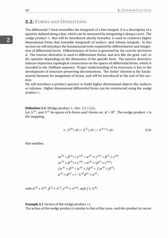
The differential 1-form resembles the integrand of a line integral. It is a description of aquantity defined along a line, which can be measured by integrating it along a curve. Thewedge product ∧, that will be introduced shortly hereafter, is used to construct higherdimensional forms that resemble integrands of surface- and volume integrals. In thissection we will introduce the fundamental tools required for differentiation and integra-tion of differential forms. Differentiation of forms is governed by the exterior derivatived . The exterior derivative is used to differentiate forms, and acts like the grad, curl, ordiv operator depending on the dimension of the specific form. The exterior derivativeinduces important topological connections on the spaces of differential forms, which isencoded in the DeRham sequence. Proper understanding of its structures is key to thedevelopment of structure-preserving discretisations. The Stokes’ theorem is the funda-mental theorem for integration of forms, and will be introduced at the end of this sec-tion.We will introduce a product operator to build higher dimensional objects like surfacesor volumes. Higher dimensional differential forms can be constructed using the wedgeproduct ∧.
Definition 2.4 (Wedge product ∧, (Sec. 2.5 [18])).Let Λ(k), and Λ(l ) be spaces of k-forms and l-forms on M ⊂ Rn . The wedge product ∧ isthe mapping,
∧ :Λ(k)(M )×Λ(l )(M ) →Λ(k+l )(M ) (2.9)
that satisfies,
(α(k) +β(l ))∧γ(m) =α(k) ∧γ(m) +β(l ) ∧γ(m)
(α(k) ∧β(l ))∧γ(m) =α(k) ∧ (β(l ) ∧γ(m))
f α(k) ∧β(l ) =α(k) ∧ f β(l ) = f (α(k) ∧β(l ))
α(k) ∧β(l ) = (−1)klβ(l ) ∧α(k),
with α(k) ∈Λ(k),β(l ) ∈Λ(l ),γ(m) ∈Λ(m), and f ∈Λ(0).
Example 2.1 (Action of the wedge product ∧).The action of the wedge product is similar to that of the cross- and dot-product in vector

2.2. FORMS AND OPERATIONS
2
11
calculus. Consider 1-forms α(1),β(1) ∈Λ1(M ) with M ⊂R3.
example 1:
d x1 ∧d x1 =−d x1 ∧d x1
⇔ d x1 ∧d x1 = 0
example 2:
α(1) ∧β(1) = (α1d x1 +α2d x2 +α3d x3)∧ (β1d x1 +β2d x2 +β3d x3)
=α1β2d x1 ∧d x2 +α1β3d x1 ∧d x3
+α2β1d x2 ∧d x1 +α2β3d x2 ∧d x3
+α3β1d x3 ∧d x1 +α3β2d x3 ∧d x2
= (α1β2 −α2β1)d x1 ∧d x2
+ (α2β3 −α3β2)d x2 ∧d x3
+ (α3β1 −α1β3)d x3 ∧d x1
example 3:
α(1) ∧β(1) ∧γ(1) = (α1β2γ3 −α2β1γ3)d x1 ∧d x2 ∧d x3
+ (α2β3γ1 −α3β2γ1)d x2 ∧d x3 ∧d x1
+ (α3β1γ2 −α1β3γ2)d x3 ∧d x1 ∧d x2
= det
∣∣∣∣∣∣α1 α2 α3
β1 β2 β3
γ1 γ2 γ3
∣∣∣∣∣∣d x1 ∧d x2 ∧d x3
Note that the result α(1) ∧β(1) is a 2-form with components similar to a ×b, which de-scribes a surface in vector calculus. Furthermore, α(1) ∧β(1) ∧γ(1) is a 3-form with com-ponents similar to a×b ·c , which describes a volume (parallelepiped) in vector calculus.
The example reveals a connection between differential forms and geometric objects.Moreover, we observe that forms resemble integrands of line-, surface-, and volume in-tegrals. In M (R3) we associate 3-forms with volumes, 2-forms with surfaces, 1-formswith lines, and 0-forms with points. Each differentiable k-form can be interpreted assome quantity that is to be measured (integrated) in some structure, e.g. flux is mea-sured through surface, and density in volume, and so on. Each physical quantity alsohas some natural orientation with respect to its underlying structure. We distinguish be-tween tangential (inner-oriented) forms, and normal (outer-oriented) forms (sec. 28 ofBurke [19]). A flux is defined normal through a surface, while vorticity is defined tan-gential to the surface. Further elaboration on the physical interpretation of differentialforms will follow in section 2.5. We present some examples.

2
12 2. EXTERIOR CALCULUS
Λ(k) geometry exampleΛ(0) points pressure p(0) = p(x, y, z)Λ(1) lines velocity v (1) = vx (x, y, z)d x + vy (x, y, z)d y + vz (x, y, z)d zΛ(2) surfaces flux σ(2) =σz (x, y, z)d x ∧d y
+σy (x, y, z)d z ∧d x +σx (x, y, z)d y ∧d zΛ(3) volumes density ρ(3) = ρ(x, y, z)d x ∧d y ∧d z.
Definition 2.5 (Exterior derivative d , (Sec. 2.6 [18])).Differentiation of differential forms is governed by the exterior derivative d . The exteriorderivative d is the mapping,
d :Λ(k)(M ) →Λ(k+1)(M ), (2.10)
satisfying,
d(α(k) +β(k)) = dα(k) +dβ(k)
d(α(k) ∧β(m)) = dα(k) ∧β(m) + (−1)kα(k) ∧dβ(m)
d 2α(k) := d dα(k) = 0,
The action of the exterior derivative on a 0-form α(0) ∈Λ(0) is given by,
dα(0) :=n∑
i=1
∂α
∂xid xi . (2.11)
The exterior derivative generalises the grad,curl, and div operators from multivariatecalculus. Furthermore, the fact that d 2 = 0, known as the nilpotency property, is equiv-alent to the curl grad = 0 and div curl = 0 relations. The exterior derivative defines asequence of mappings, known as the DeRham complex. For M ⊂Rn we have
R Λ(0) Λ(1) · · · Λ(n) ;d d d d
The action of the exterior derivative on various forms is shown below.
Example 2.2 (Action of the exterior derivative d in R3).The action of the exterior derivative is very similar to the grad, curl and div operators.Using the properties of the wedge product ∧, and the exterior derivative d , we find forM ⊂R3,

2.2. FORMS AND OPERATIONS
2
13
0-form:
dφ(0) = ∂φ
∂x1d x1 + ∂φ
∂x2d x2 + ∂φ
∂x3d x3
1-form:
du(1) =(∂u1
∂x1d x1 + ∂u1
∂x2d x2 + ∂u1
∂x3d x3
)∧d x1
+(∂u2
∂x1d x1 + ∂u2
∂x2d x2 + ∂u2
∂x3d x3
)∧d x2
+(∂u3
∂x1d x1 + ∂u3
∂x2d x2 + ∂u3
∂x3d x3
)∧d x3
=(∂u3
∂x2− ∂u2
∂x3
)d x2 ∧d x3 +
(∂u1
∂x3− ∂u3
∂x1
)d x3 ∧d x1 +
(∂u2
∂x1− ∂u1
∂x2
)d x1 ∧d x2
2-form:
dω(2) =(∂ω1
∂x1d x1 + ∂ω1
∂x2d x2 + ∂ω1
∂x3d x3
)∧d x2 ∧d x3
+(∂ω2
∂x1d x1 + ∂ω2
∂x2d x2 + ∂ω2
∂x3d x3
)∧d x3 ∧d x1
+(∂ω3
∂x1d x1 + ∂ω3
∂x2d x2 + ∂ω3
∂x3d x3
)∧d x2 ∧d x3
=(∂ω1
∂x1+ ∂ω2
∂x2+ ∂ω3
∂x3
)d x1 ∧d x2 ∧d x3
Hence dφ(0) defines a 1-form with components of grad operator in Cartesian coordi-nates, du(1) defines a 2-form with components of curl operator, and dω(2) defines a 3-form with component of the div operator.Important topological connections are encoded in the exterior derivative and the DeR-ham sequence. Connections between exterior derivative’s kernel and range, subspacesof the Λ(k)′ s, have an important role in the existence and uniqueness of PDE solutions.More on the structure of the DeRham sequence can be found in Appendix A. From thenilpotency of the exterior derivative it follows that if dα(k) =β(k+1), then dβ(k+1) = 0. Theconverse is true on contractible manifolds. Contractible manifolds can be continuouslyreduced to a point. Examples include any (star) domain in Euclidean space.
Theorem 2.1 (Poincaré Lemma, (Sec. 5.4 [18])).Let β(k) be a k-form on contractible manifold M , such that dβ(k) = 0. There exists a non-
unique α(k−1), such that,
dα(k−1) =β(k). (2.12)
Often α(k−1) is referred to as a potential function.
The theorem proofs existence of solutions for balancing relations is physics. Theserelations, often of the form grad(φ) = f , curl(~ω) = ~g , and div(~v) = h, are fundamental in

2
14 2. EXTERIOR CALCULUS
the description physics. Furthermore, note that the theorem proofs existence of poten-tials for every volume form, as dρ(n) = 0 for any volume form ρ(n). In vector calculus thisresult is known as the surjectiveness of the div operator.
Example 2.3 (Potential flow).Irrotational (inviscid) flow satisfies ∇×~V = 0, or in terms of differential geometry, d v (1) =0. Hence by the Poincaré lemma, there exists a velocity potential function φ(0) ∈Λ(0) s.t.dφ(0) = v (1). Flow solutions satisfying dφ(0) = v (1) are known as potential flow solutions.We will discuss potential flow in more detail in section 2.5.
We measure a differential form by pairing it with an equidimensional submanifold,e.g. a 2-form is measured by pairing it with some surface S, a 3-form with some volumeV , and so on. We present a few examples.
Λ(k) geometry exampleΛ(0) point: x pressure P = ∫
x p(0)
Λ(1) curve: γ circulation Γ= ∮γ v (1)
Λ(2) surface: S flux Φ= ∫S σ
(2)
Λ(3) volume: V mass M = ∫V ρ
(3).
Integration is governed through the generalised Stokes’ theorem .
Theorem 2.2. Generalised Stokes’ Theorem, (Sec. 3.3 [18])Let α(k) ∈Λ(k) be a k-form, and M be a (k +1)-dimensional submanifold. Then,∫
Mdα(k) =
∫∂M
α(k). (2.13)
The theorem generalises the classical Stokes’, Green’s and divergence theorem frommultivariate calculus, as well as the fundamental theorem of calculus. The theoremstates that the boundary operator ∂ is the formal adjoint of the exterior derivative d ,i.e.
⟨M ,dα(k)⟩ = ⟨∂M ,α(k)⟩. (2.14)
Note that this result is purely topological. In the next section we will introduce the dis-crete analogue of the generalised stokes theorem.
2.3. CHAINS AND COCHAINSIn discretisation techniques we find the formation of some a cell complex, i.e. a grid ofvertices, edges, faces, and volumes. These components, known as k-cells. Using k-cellswe can define discrete counter-parts of submanifolds, chains, and differential forms,cochains. Cochains can be integrated by pairing them with chains. We can apply thegeneralised Stokes’ theorem, Equation 2.13, to these structures to derive a discrete ver-sion of the exterior derivative, the coboundary operator δ. The coboundary operatorsatisfies the same topological structure as the exterior derivative. Its action is encodedin incidence matrices E(k,k−1). These incidence matrices are the foundation of our dis-cretisation approach.

2.3. CHAINS AND COCHAINS
2
15
Definition 2.6 (k-cell, (Appx. B.a [18])).A k-cell, τ(k), is a k-dimensional submanifold of n-dimensional manifold M which ishomeomorphic to k-dimensional unit ball.
Essentially k-cells are k-dimensional contractible spatial objects. From here on wewill form a grid of k-cells which will act as a discrete manifold on which we can definea discrete counterpart of differential forms. Grids are generally constructed using sim-plexes, or simplicial structures. In this work we follow [6, 20] and use k-dimensionalcuboids, k-dimensional objects for which there exists a bijection to the unit k-cube,x ∈ [−1,1]k . These cuboids are convenient because of their ability to hold tensor-product structures, and because Gaussian quadrature rules are defined on its interior.
Example 2.4 (n-dimensional cuboids).A 3-dimensional cuboid is a convex polytope bounded by 6 quadrilateral faces, each faceis bounded by 4 edges, and each edge is bounded by 2 nodes. Hence each 3-dimensionalcuboid consists of 8,12,6,1 0,1,2,3-dimensional objects. A 4-dimensional cuboidconsists of 16,32,24,8,1 0,1,2,3,4-dimensional objects.
Definition 2.7 (Cell Complex, (Appx. B.a [18])).A cell complex D on a n-dimensional differentiable manifold M is a finite collection ofsets of n,n −1, · · · ,0-cells such that,
i The collection of n-cells form a cover M .
ii Every face of a k-cell is contained in D.
iii Any two k-cells τ(k),σ(k) ∈D,
τ(k) ∩σ(k) =
υ(k−1), i.e. τ(k),σ(k) share a boundary υ(k−1)
σ(k) = τ(k), i.e. they indicate the same k-cell
;(2.15)
The cell complex forms the collection of nodes, lines, surfaces, volumes that is equiv-alent to grid structures in numerical methods. It will also form a discrete manifold struc-ture on which we can perform numerical analysis. For a cell complex to act like a mani-fold, we will need to provide orientation to its k-cells. Oriented k-cells act as a basis. Setsof oriented k-cells are known as k-chains. These k-chains can be interpreted as discretesubmanifolds.
Definition 2.8 (k-Chains c (k), (Appx. B.a [18])).The space of k-chains on a cell complex D, denoted by C(k)(D), is the space of all sets ofk-cells. Hence each k-chain c (k) ∈C(k)(D) can be written as,
c (k) =∑
ic iτ(k),i , with τ(k) ∈D, (2.16)
with c i the expansion coefficients. We use k-chains to describe k-dimensional pathsthrough oriented cell complexes. In our analysis we consider coefficients c i ∈ 0,±1,where c i = ±1 provides relative orientation of the i -th k-cell with respect to a globalorientation, and c i = 0 indicates that i -th k-cell is not within the considered path.

2
16 2. EXTERIOR CALCULUS
Example 2.5 (1-chains).Consider the oriented cell complex D shown in Figure 2.3. Closed paths around surfacess1, s2 are described by 1-chains c (1),c (2) ∈C(1)(D),
c 1 = l1 + l6 − l3 − l5,
c 2 = l2 + l7 − l4 − l6.
The space of C(1)(D) is a linear vector space, hence we are able to add c ′(k)s to construct
new paths. For example, c (1) + c (2) describes the path that encloses s1 ∪ s2. Next, weintroduce the boundary operator δ, which relates a k-chain to its boundary (k −1)-cells.
Definition 2.9 (Boundary operator ∂, (Appx. B.a [18])).The boundary operator is the mapping,
∂ : C(k) →C(k−1), ∂c (k) =∑
jc j∂τ(k), j , (2.17)
where the boundary operator ∂ acting on the j -th k-cell τ(k), j is given by,
∂τ(k), j =∑
ie i
jτ(k−1),i ,
with,
e ij =
+1, if orientation of τ(k−1),i is the same as the boundary of τ(k), j
−1, if orientation of τ(k−1),i is opposed to that of the boundary of τ(k), j
0, if τ(k−1),i is no face of τ(k), j
.
The boundary operator acting on a k-cell is encoded in an incidence matrix E(k−1,k) with
entries E(k−1,k)(i , j ) given by e ji . The boundary operator satisfies ∀c (k) ∈C(k)(D),
∂c (0) =0,
∂∂c (k) =0,
for which the latter property translates to matrix notation as (E(k−2,k−1)E(k−1,k))c (k) = 0.Finally, the boundary operator defines a sequence of mappings
; C(0) C(1) · · · C(n) R∂ ∂ ∂ ∂
Example 2.6 (Boundary operator ∂). Consider again the oriented cell complex D in Fig-ure 2.3. We find that
∂s1 = l1 + l6 − l3 − l5,
∂s2 = l2 + l7 − l4 − l6.

2.3. CHAINS AND COCHAINS
2
17
Now take chains c (2) = [s1, s2]T , c (1) = [l1, l2, · · · , l7]T , and c (0) = [p1, p2, · · · , p6]T . Wecould obtain c (1) through c (1) = E(1,2)c (2), and c (0) through c (0) = E(0,1)c (1), with
E(0,1) =
1 0 0 0 1 0 0−1 1 0 0 0 1 00 −1 0 0 0 0 10 0 1 0 −1 0 00 0 −1 1 0 −1 00 0 0 −1 0 0 −1
, E(1,2) =
1 00 1−1 00 −1−1 01 −10 1
,
where, for example, the 6-th row of E(1,2) corresponds to l6 for which orientation is similarto the face of s1, but opposite to the face of s2. One could check that E(0,1)E(1,2)c (2) = 0, i.e.the nilpotency ∂∂c (2) = 0 of the boundary operator is exact in these discrete structures.This is of great importance, as it will preserve the topological relations between exactand closed forms, introduced in the previous section, in the discrete setting. We will nowintroduce the discrete differential forms, known as cochains , which assign real values tothe k-chains introduced.
s1 s2
l1
l3
l2
l4
l5 l6 l7
p1
p4
p2
p5
p3
p6
Figure 2.3: Cell complex D on a 2-dimensional manifold. Positive orientation of k-cells is indicated bydirection of the arrows.
Definition 2.10 (k-Cochains c (k), (Appx. B.b [18])).The space of k-cochains on a cell complex D, denoted by C (k)(D), is the space that isdual to the space of k-chains C(k)(D). A k-cochain c (k) expands in basis τ(k),
c (k) =∑i
ciτ(k),i , (2.18)
where τ(k) is dual to a k-cell such that τ(k),i (τ(k), j ) = δij . The action of a k-cochain is the

2
18 2. EXTERIOR CALCULUS
mapping c (k) : C(k)(D) →R, with
⟨c (k),c (k)⟩ := c (k)(c (k)) =∑
i
∑j
ci c jτ(k),iτ(k), j =∑
ici c j .
Note that we could have chosen any other dual basis τ(k),i that spans C (k). Cochainsact as discrete differential forms, as will be shown. We now introduce the coboundaryoperator δ, which is the discrete equivalent of the differential operator.
Definition 2.11 (Coboundary operator δ).The coboundary operator δ : C (k) →C (k+1) is the formal adjoint of the boundary opera-
tor,
⟨c (k),δc (k)⟩ = ⟨∂c (k),c (k)⟩ . (2.19)
It follows that we can also encode the action of the coboundary operator in an incidencematrix,
⟨E(k−1,k)c (k),c (k)⟩ = ⟨c (k), (E(k−1,k))T c (k)⟩ .
Hence we define,
E(k,k−1) := (E(k−1,k))T . (2.20)
The coboundary operator inherits nilpotency property δδ = 0 from the boundary op-erator,
⟨c (k),δδc (k)⟩ 2.19= ⟨∂c (k),δc (k)⟩ 2.19= ⟨∂∂c (k),c (k)⟩ = 0,
and it defines a sequence of mappings,
R C (0) C (1) · · · C (n) ;.δ δ δ δ
We can now connect the continuous differential forms from the previous section tothe discrete cochain structures defined in this section.
Example 2.7 (Discretisation of v (1) = dφ(0)).Consider again the oriented cell complex shown in Figure 2.3. Now consider the equa-
tion v (1) = dφ(0), defined on some manifold that is covered by the cell-complex. We canintegrate over any line element l and use Stokes’s theorem to find,∫
lv (1) =
∫l
dφ(0) 2.13=∫∂l1
φ(0)
Next we discretise the variables v (1),φ(0) through integration,
v (1) =[∫
l1
v (1),∫
l2
v (1), · · · ,∫
l7
v (1)]T
,
φ(0) =[φ(0)(p1),φ(0)(p2), · · · ,φ(0)(p6)
]T.

2.3. CHAINS AND COCHAINS
2
19
The v (1), and φ(0) are cochains, each coefficient assigns a real value to an oriented k-cell, just as a differential form assigns a real value to a manifold. We can now solve thediscrete equation using the coboundary operator. Consider any 1-chain c (1), we find∫
c (1)
v (1) =∫∂c (1)
φ(0)
⇔ ⟨v (1),c (1)⟩ = ⟨φ(0),∂c (1)⟩ = ⟨δφ(0),c (1)⟩⇔ ⟨v (1) −E(1,0)φ(0),c (1)⟩ = 0.
So we can solve the equation by evaluating v (1) = E(1,0)φ(0). The result is exact, no ap-proximation has been made in this derivation, although information of the continuousforms have been lost in the process. In fact, any relation of the form α(k) = dβ(k−1) canbe discretised and solved using this approach, which preserves exactness of the exteriorderivative, Appendix A.
We are able to preserve the exactness of the topological structure of our equationswhen we go to the discrete setting. However, the discretisation of the continuous formsto the discrete cochains came at a cost. We were able to conserve the global quantity atthe cost of information concerning local behaviour. If we want to go back to a continu-ous form, we need to reconstruct the solution, performing some kind of interpolation.Bochev and Hyman introduced a framework to encode this process [6], which dependson the reduction- and reconstruction-operators.
Definition 2.12 (Reduction Operator R(k)).The reduction operator R(k) is a mapping
R(k) :Λ(k)(M ) →C (k)(D), (2.21)
that satisfies commutativity δR(k) =R(k+1)d , illustrated below.
Λ(k) Λ(k+1)
C (k) C (k+1)
d
δ
R(k+1)R(k)
Definition 2.13 (Reconstruction Operator I (k)).The reconstruction operator I (k) is a mapping
I (k) : C (k)(D) →Λ(k)h (M ), (2.22)
where Λ(k)h (M ) ⊂ Λ(k)(M ) is an approximate finite-dimensional subspace of Λ(k)(M ).
The reconstruction operator needs to satisfy the same commutative property, δI (k) =I (k+1)d , illustrated below.

2
20 2. EXTERIOR CALCULUS
C (k) C (k+1)
Λ(k)h Λ(k+1)
h
δ
d
I (k+1)I (k)
Using the reduction and reconstruction operators it is possible to describe the dis-cretisation process through the commuting diagram in Figure 2.4. Successful discretisa-tion needs to satisfy the following conditions;
i Consistency condition, R(k)I (k) = I ,
ii Approximation condition, I (k)R(k) = I +O (hp+1),
where h is some measure of grid size, and p the polynomial order of the approximation.We can use operators R, I to define discrete operators acting on cochain c (k) ∈ C (k).Consider any operator F acting on Λ(k), s.t. F :Λ(k) →Λ(l ). We can then define discreteoperator Fh through
Fh c (k) :=R(k)FI (l )c (k).
Λ(k) Λ(k+1)
C (k) C (k+1)
Λ(k)h Λ(k+1)
h
d
d
δ
R(k+1)R(k)
R(k+1)R(k) I (k+1)I (k)
Figure 2.4: Commuting diagram of the reconstruction and reduction operators R and I .
Classic discretisation techniques can be described through the reduction and recon-struction operators. In finite differencing techniques, one reconstructs using Taylor se-ries expansion, while in finite volume techniques, one often reconstructs using polyno-mial interpolation. In finite element techniques, forms are reconstructed using basisfunctions. In finite differencing, and finite volume techniques, an explicit grid is gen-erated, and one can reduce the continuous forms using integration, as in Example 2.7.Grids structures in finite element techniques are less obvious. Explicit reduction in finiteelement techniques can be performed using dual basis functions or projection opera-tors.

2.4. THE CODIFFERENTIAL AND THE INNER PRODUCT
2
21
2.4. THE CODIFFERENTIAL AND THE INNER PRODUCT
So far we have treated relations that are topological. In the previous section, we haveshown that the exterior derivative d can be discretised without loss of its structure. Inthis section we will introduce operations that depend on metric. In the discrete settinglocal geometry is approximated on some mesh, which induces an approximation errorfor metric-dependent relations. Fundamental is the Hodge-? operator, which maps anoriented form to its corresponding dual-oriented form. The Hodge-? operator definesan inner-product, which is a vital tool in variational analysis.
Definition 2.14 (Hodge-? operator, (Sec. 14.1 [18])).The Hodge-? operator in M ⊂Rn is a mapping ? :Λ(k) →Λ(n−k) with,
?α(x1, · · · , xn)d xi1 ∧·· ·∧d xik = sign ·α(x1, · · · , xn)d x j1 ∧·· ·∧d x jn−k , (2.23)
where i1, · · · ik ⊆ 1, · · · ,n and j1, · · · jn−k its complement, and
sign =− , if j1, · · · , jn−k , i1, · · · , ik is an even permutation of 1, · · · ,n
+ , else.
When applied twice to a differential k-form we find that ??α(k) = (−1)k(n−k)α(k). TheHodge-? defines a complex of sequences of mappings, known as the double DeRhamcomplex , Figure 2.5.
R Λ(0) Λ(1) · · · Λ(n) ;
; Λ(n) Λ(n−1) · · · Λ(0) R
d d d d
d d d d
? ? ?
Figure 2.5: Double DeRham complex; two dual DeRham sequences are connected through the Hodge-?operator.
Example 2.8 (Geometrical Interpretation of the Hodge-? operator).The Hodge-? transforms differential forms to their dual forms . Its action doesn’t affectthe magnitude or direction of the components, but maps the basis to its dual configura-

2
22 2. EXTERIOR CALCULUS
tion. Some examples are given,
R2 :
?1 = d x1 ∧d x2
?d x1 = d x2
?d x2 =−d x1
R3 :
?1 = d x1 ∧d x2 ∧d x3
?d x1 = d x2 ∧d x3
?d x2 ∧d x1 =−d x3
Now consider the case R2, for which the double DeRham complex is shown in Figure 2.6.Any point value becomes a face value and vice versa. A value associated along a line,becomes a value associated through a line.
Λ(0) Λ(1) Λ(2)
Λ(2) Λ(1) Λ(0)
d d d
d d d d
? ? ?
R ∅
∅ R
l
l
p
s
s
p
Figure 2.6: Double DeRham complex in R2.
The double-DeRham complex shows that we can identify two distinct orientationsof a physical quantity on a geometric object. The top row in Figure 2.6 corresponds toinner-orientated object (or tangent orientated). From left to right we observe a source ina point, some quantity along a line, rotation in a surface. The bottom row correspondsto outer-oriented objects (or normal oriented). Here we see source through a face, fluxthrough a surface, rotation around a point. Topological connections are shown horizon-tally, while metric-dependent relations are shown vertically.
Definition 2.15 (Inner Product (·, ·)M , (Sec. 14.1 [18])).The Hodge-? operator defines an L2-inner product (·, ·)M :Λ(k) ×Λ(k) →R by
(α(k),β(k))M :=∫Mα(k) ∧?β(k), (2.24)
with α(k),β(k) ∈Λ(k) on M .

2.4. THE CODIFFERENTIAL AND THE INNER PRODUCT
2
23
The inner product is essential in variational analysis, and plays a vital role in theconstruction of a finite-elements framework as we will see in the next chapter, chapter 3.With the Hodge-? operator we can define the adjoint of the differential operator, thecodifferential d∗ .
Definition 2.16 (Codifferential d∗, (Sec. 14.1 [18])).The codifferential d∗ is a mapping d∗ :Λ(k)(M ) →Λ(k−1)(M ) for which
d∗α(k) = (−1)n(k−1)+1?d ?α(k) (2.25)
The codifferential defines a sequence of mappings, known as the DeRham complex,which connects k +1-forms to k-forms. For M ⊂Rn we have
; Λ0 Λ1 · · · Λn Rd∗ d∗ d∗ d∗
It’s easy to see that d∗ is nilpotent, i.e. d∗d∗ = 0 (using the ?? and d 2 properties).
Example 2.9 (Action of codifferential d∗ in R3).The action of the exterior derivative is similar to the div, curl and grad operators. Usingthe properties of the wedge product ∧, and the exterior derivative d , we find for M ⊂R3,
1-form:
d∗u(1) =−[∂u1
∂x1+ ∂u2
∂x2+ ∂u3
∂x3
]2-form:
d∗ω(2) = (−1)n+1[(∂ω3
∂x2− ∂ω2
∂x3
)d x1 +
(∂ω1
∂x3− ∂ω3
∂x1
)d x2 +
(∂ω2
∂x1− ∂ω1
∂x2
)d x3
]2-form:
d∗ρ(3) =−[∂ρ
∂x1d x2 ∧d x3 + ∂ρ
∂x2d x3 ∧d x1 + ∂ρ
∂x3d x1 ∧d x2
]
Hence d∗u(1) defines a 0-form with components of div operator, d∗ω(2) defines a 1-formwith components of curl operator, and d∗ρ(3) defines a 2-form with component of thegrad operator. The codifferential is the adjoint of the exterior derivative.
Theorem 2.3 (Integration-by-parts, (Sec. 14.1 [18])).For forms α(k−1) ∈Λ(k−1), and β(k) ∈Λ(k), we have the relation,
(α(k−1),d∗β(k))M = (dα(k−1),β(k))M − (α(k−1),β(k))∂M , (2.26)
Now any differential k-form can be decomposed in orthogonal components tangentialand normal to the boundary, i.e. α(k) =αnd xn+αt d xt . Hence we can evaluate the bound-ary integral in terms of tangential and normal components of α(k−1),β(k),
(α(k−1),β(k))∂M =∫∂M
⟨αt ,βn⟩dΓ. (2.27)

2
24 2. EXTERIOR CALCULUS
Proof can be found in Appendix B. We will often use Theorem 2.3 to reduce continuityconstraint on our solution space, or to get rid of the co-differential.
We combine the exterior derivative and the codifferential operator to define the Laplace-DeRham operator, which is a generalised Laplace operator for k-forms.
Definition 2.17 (Laplace-de-Rham Operator, (Sec. 14.2 [18])).For any k-form we define the Laplace-de-Rham operator ∆ :Λ(k) →Λ(k) as
∆α(k) := dd∗α(k) +d∗dα(k) = (d +d∗)2α(k) (2.28)
Because d∗β(0) = 0 for any 0-formβ(0), the Laplace-DeRham operator acting on a 0-formreduces to ∆ = d∗d , which is the equivalence of the scalar Laplacian. The operatorsreduces to ∆= dd∗ when applied to a volume n-form.
The codifferential governs the a topological structure that mirrors the structure of theexterior derivative. It governs existence of solutions analogue to the Poincaré lemma,Equation 2.12. In Appendix A we combine properties of both operators to derive theHodge decomposition, which states there exists an unique decomposition in orthogonalcomplements for each k-form.
Theorem 2.4 (Hodge decomposition, (Sec. 14.2 [18])).For any k-form on a closed manifold M there exists an unique decomposition
α(k) = dφ(k−1) +d∗ψ(k+1) +h(k), (2.29)
where h(k) is a harmonic form, i.e. ∆h(k) = 0. Note that this doesn’t imply uniqueness ofφ(k−1) and ψ(k+1). On a contractable manifold the space of harmonic forms is empty, i.e.h(k) = 0.
2.5. POISSON PROBLEMSThere exists one-to-one correspondence between PDE’s described using vector calcu-lus and differential geometry. In multivariate calculus we distinguish between physicalvariables associated with scalars and those associated with vectors. In differential ge-ometry we associate physical variables with points, lines, surfaces, and volumes. Anyscalar function can be used to describe a point or volume (0,3)-form in R3, and any vec-tor function can be used to describe a line or surface (1,2)-form. The duality between apoint and a volume, and that between a surface and a line is encoded in the Hodge ?-operator. Let’s analyse the example of potential flow, which we introduced in section 2.2.
Example 2.10 (Potential flow in R2).The velocity field can be interpreted as a field of lines along which fluid parcels aretransported. Hence we can associate a 1-form with velocity, i.e. v (1). Now the quantityω(2) = d v (1) is known as vorticity and is a measure of rotation within the flow. In the caseof irrotational flow, i.e. ω(2) = 0 in our domain, we would get d v (1) = 0. Assuming that thedomain is simply connected, there exists a potential function φ(0) such that dφ(0) = v (1)
(Theorem 2.1).
2.5. POISSON PROBLEMS
2
25
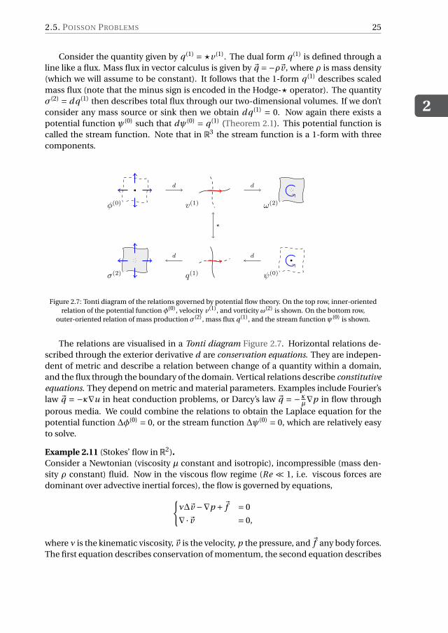
Consider the quantity given by q (1) = ?v (1). The dual form q (1) is defined through aline like a flux. Mass flux in vector calculus is given by ~q =−ρ~v , where ρ is mass density(which we will assume to be constant). It follows that the 1-form q (1) describes scaledmass flux (note that the minus sign is encoded in the Hodge-? operator). The quantityσ(2) = d q (1) then describes total flux through our two-dimensional volumes. If we don’tconsider any mass source or sink then we obtain d q (1) = 0. Now again there exists apotential function ψ(0) such that dψ(0) = q (1) (Theorem 2.1). This potential function iscalled the stream function. Note that in R3 the stream function is a 1-form with threecomponents.
φ(0) v(1) ω(2)
σ(2) q(1) ψ(0)
d d
d d
?
Figure 2.7: Tonti diagram of the relations governed by potential flow theory. On the top row, inner-orientedrelation of the potential function φ(0), velocity v (1), and vorticity ω(2) is shown. On the bottom row,
outer-oriented relation of mass production σ(2), mass flux q(1), and the stream function ψ(0) is shown.
The relations are visualised in a Tonti diagram Figure 2.7. Horizontal relations de-scribed through the exterior derivative d are conservation equations. They are indepen-dent of metric and describe a relation between change of a quantity within a domain,and the flux through the boundary of the domain. Vertical relations describe constitutiveequations. They depend on metric and material parameters. Examples include Fourier’slaw ~q = −κ∇u in heat conduction problems, or Darcy’s law ~q = −κ
µ∇p in flow throughporous media. We could combine the relations to obtain the Laplace equation for thepotential function ∆φ(0) = 0, or the stream function ∆ψ(0) = 0, which are relatively easyto solve.
Example 2.11 (Stokes’ flow in R2).Consider a Newtonian (viscosity µ constant and isotropic), incompressible (mass den-sity ρ constant) fluid. Now in the viscous flow regime (Re ¿ 1, i.e. viscous forces aredominant over advective inertial forces), the flow is governed by equations,
ν∆~v −∇p +~f = 0
∇·~v = 0,
where ν is the kinematic viscosity,~v is the velocity, p the pressure, and ~f any body forces.The first equation describes conservation of momentum, the second equation describes

2
26 2. EXTERIOR CALCULUS
conservation of mass. We can translate to the language of differential geometry. Weobtain,
νd∗d v (1) +d p(0) = f (1)
−d∗v (1) = 0.
We can obtain an equivalent dual formulation of these equations by pre-multiplying theequations with the Hodge-?, define dual forms, i.e. q (1) =?v (1), p(0) =?p(2), and f (1) =?g (1), and use the identities of d∗, d and ? to simplify the result. For the Stokes’ flowequations one obtains,
νdd∗q (1) −d∗p(2) = g (1)
d q (1) = 0.
The advantage of this formulation, is that the mass conservation constraint d q (1) = 0depends on the exterior derivative d . This means that a discretisation based on this for-mulation can be made such that it satisfies conservation of mass exactly pointwise (usingthe incidence matrices introduced in section 2.3). Structure preserving spectral elementsolution methods for the Stokes’ flow problem are studied in [21]. Their discretisationsatisfies pointwise divergence-free solution.
The last example showed that formulation has consequences in the discrete set-ting. We can choose the formulation such that certain relations are satisfied stronglypointwise, while others are weakly satisfied. The choice of formulation will also have aconsequence on the boundary conditions. Some boundary condition may be enforcedstrongly (essential) in one formulation, while it may be enforced weakly (natural) in adifferent one.
So far we have not considered the possibility of arbitrary physical geometries. Often,the quantity of interest will be defined on a geometry through a mapping. In the finite-element method we will need to pull-back differential k-forms to some parent domainon which the numerical integration rules are defined. The pull-back operator commu-tates with the exterior derivative. In Appendix C we derive appropriate transformationsfor each k. These relations conserve the topological structure of the exterior derivativeon arbitrary domains.
2.6. SUMMARY OF RESULTSAnalysis of PDE’s through exterior calculus enables us to distinguish between relationsthat depend on metric, and those that are topological. Topological relations can be de-scribed by algebraic equations, which can be satisfied exactly in the discrete setting.Proper discretisation of these relations guarantees numerical stability, and exact be-haviour of simulated physics.
The exterior derivative d is a topological operator, which describes derivatives of dif-ferential forms analogous to the grad-, curl-, and div- operators. In the discrete settingit can be satisfied without error by construction of incidence matrices. This construc-tion preserves the kernel structure of the exterior derivative, which governs existence of

2.6. SUMMARY OF RESULTS
2
27
PDE solutions. The kernel structure of the exterior derivative is encoded in the DeRhamcomplex.
R Λ(0) Λ(1) Λ(2) Λ(3) ;d d d d
The Hodge-? is a metric-dependent operator, which maps differential forms to theirdual representation. It is used together with the exterior derivative d to describe ellip-tic PDE’s. Its action needs to be approximated in the discrete setting. In finite volumetechniques its action is approximated through construction of a dual grid, whereas infinite-element techniques is is approximated through inner-product relations. Finally,the Hodge-? allows us to map PDE’s to a favourable configuration, in which certain re-lations or boundary conditions can be satisfied exactly.


3STRUCTURE PRESERVING
ISOGEOMETRIC ANALYSIS
"Don’t worry, everything will B-spline"
We can use powerful tools from functional analysis to prove well-posedness of ellip-tic PDE problems. In this approach one derives a weak formulation of the PDE problemby taking the inner product with a test function. The weak formulation of the prob-lem can be converted to a discrete problem by introducing a finite-dimensional basis inwhich the unknowns and test-function can be expanded. In isogeometric analysis splinebases from computer aided design are used to discretise the problem. In this chapterwe will introduce concepts from functional analysis, and explain the fundamentals ofisogeometric analysis. We will construct a discretisation framework using splines that iscompatible with the DeRham complex.
Weak formulations of elliptic PDE problems that define a symmetric bilinear opera-tor have been discretised successfully using the finite element method. Mixed type for-mulations however have posed difficulties. Such problems are known for spurious oscil-lations within the numerical solution. In order to cope with these oscillations penalisingtechniques were introduced, which in turn have a negative effect on the accuracy, (Sec.6.3 [2]). Classical is the work by Brezzi on stability requirements for these mixed-type for-mulations [22]. It was shown that spurious oscillations do not appear when inf-sub sta-ble finite element spaces are used. Using the concepts introduced in chapter 2, we deriveappropriate basis functions. The resulting method doesn’t require penalising techniquesfor stability, as shown by [5, 11, 23].
In section 3.1 we introduce fundamentals of functional analysis and introduce a DeR-ham sequence of Sobolev spaces. We will derive symmetric and mixed formulations ofthe Poisson problem, and prove well-posedness for both problem types. Furthermorewe will explain how we can discretise the problem by considering finite-dimensionalSobolev subspaces. Bézier, B-spline, and NURBS- polynomial bases will be introducedin the context of isogeometric analaysis in section 3.2. These basis functions will be used
29

3
30 3. STRUCTURE PRESERVING ISOGEOMETRIC ANALYSIS
to construct finite-dimensional Sobolev subspaces that are compatible with the DeR-ham complex in section 3.3. We will make a link to concepts introduced in chapter 2,and unveil the cochain structure of spline spaces. Finally, in section 3.4, we successfullydiscretise both Poisson problems using linear combinations of incidence matrices andmass matrices.
3.1. THE SOBOLEV-DERHAM COMPLEXFinite projection methods, e.g. isogeometric analysis and the finite element method,can be derived from variational analysis. In this approach one constructs a weak formu-lation of the PDE problem by taking the inner product with some test function. Well-posedness of these problems can be proven by selecting appropriate trial- and solutionspaces. In this section we construct these spaces, such that they satisfy the DeRham se-quence. We introduce the Poisson problems that will be studied in this chapter, and de-rive corresponding weak formulations. We end this section by explaining how we weakformulations can be discretised.
Consider orientable manifold Ω with tangent space T Ω and cotangent space T ∗Ω.In section 2.4 we defined an inner product on these spaces. We use the inner product todefine inner product spaces L2Λ(k).
Definition 3.1 (Inner product space L2Λ(k), (Sec. 2 [5])).Let Λ(k)(Ω) denote the space of k-forms on manifold Ω. We define the correspondingspace of square integrable forms L2Λ(k)(Ω) as,
L2Λ(k) := α(k) ∈Λ(k) : ‖α(k)‖L2Λ(k) <∞, (3.1)
where,
‖α(k)‖2L2Λ(k) =
(α(k),α(k)
)Ω=
∫Ωα(k) ∧?α(k) (3.2)
i.e. the norm defined by the inner product.
Definition 3.2 (Sobolev spaces WdΛ(k), (Sec. 2 [5])).
We define the Sobolev space WdΛ(k)(Ω) as
WdΛ(k) := α(k) ∈ L2Λ(k) : dα(k) ∈ L2Λ(k+1), (3.3)
with corresponding Sobolev norm,
‖α(k)‖2WdΛ
(k) = ‖α(k)‖2L2Λ(k) +‖dα(k)‖2
L2Λ(k+1) (3.4)
Note that WdΛ(0) is the equivalent of the Sobolov space H 1(Ω), WdΛ
(1) of H(curl;Ω),and WdΛ
(2) of H(div;Ω), i.e. descriptions of Sobolev spaces generally encountered inliterature, e.g. [11]. InΩ⊆R3 these spaces satisfy the DeRham sequence, i.e. the DeRhamSobolev complex,
WdΛ(0) WdΛ
(1) WdΛ(2) L2Λ(3)d d d
3.1. THE SOBOLEV-DERHAM COMPLEX
3
31
This construction can be mirrored to construct Sobolev spaces with respect to the cod-ifferential d∗,
Wd∗Λ(k) := α(k) ∈ L2Λ(k) : d∗α(k) ∈ L2Λ(k−1), (3.5)
with corresponding Sobolev norm,
‖α(k)‖Wd∗Λ(k) = ‖α(k)‖L2Λ(k) +‖d∗α(k)‖L2Λ(k−1) (3.6)
These spaces incorporates the existence of the DeRham complex given by
L2Λ(0) Wd∗Λ(1) Wd∗Λ(2) Wd∗Λ(3)d∗ d∗ d∗
These spaces act as trial- and solution-spaces in variational analysis of PDE prob-lems. In this approach one derives a weak formulation of the PDE problem. In thischapter we will study Poisson problems, e.g. those appearing in potential flow theory,section 2.5.
Problem 3.1 (The 0-form Poisson Problem in R2).Consider the domain Ω = [0,1]2 ⊂ R2 with boundary ∂Ω = Γd ∪Γn , where Γd ∩Γn = ;.
Given forcing f (0) ∈Λ(0), find solution ψ(0) ∈Λ(0) such that,∆ψ(0) = f (0),
ψ(0) = 0, on Γd
∂nψ(0) = 0, on Γn
(3.7)
A corresponding weak formulation of this problem can be obtained by taking the innerproduct with some test function w (0). Given forcing f (0) ∈ L2Λ(0), find solution ψ(0) ∈WdΛ
(0), such that,(d w (0),dψ(0))
Ω = (w (0), f (0))
Ω , ∀w (0) ∈WdΛ(0)0 , (3.8)
where WdΛ(0)0 is the space of compactly supported functions,
Λ(0)0 := α(0) ∈Λ(0) : with α(0) = 0 on Γd .
The derivation of this weak formulation, and a proof of well-posedness of the weak for-mulation is given in Appendix D. In the derivation of the weak formulation we usedintegration by parts, Theorem 2.3, for two reasons. In the discrete setting we will use afinite span of basis functions of a given polynomial order. Integration by parts reducescontinuity requirements on the span of basis functions. The second reason is that wenow have an expression that doesn’t contain the codifferential d∗, but only contains theexterior derivative d , which we can discretise using the framework introduced in sec-tion 2.3.

3
32 3. STRUCTURE PRESERVING ISOGEOMETRIC ANALYSIS
Problem 3.2 (The 2-form Poisson Problem in R2).Consider the domain Ω = [0,1]2 ⊂ R2 with boundary ∂Ω = Γd ∪Γn , where Γd ∩Γn = ;.
Given forcing f (2) ∈Λ(0), find solution ψ(2) ∈Λ(2) such that,∆ψ(2) = f (2),
ψ(2) = 0, on Γd
∂tψ(2) = 0, on Γn
(3.9)
As before, we could multiply with some test-function w (2), and apply integration byparts, to obtain. (
d∗w (2),d∗ψ(2))Ω = (w (2), f (2))Ω. (3.10)
This formulation won’t do us any good in the discrete setting, because it contains thecodifferential d∗. Alternatively we write Equation 3.9 as an equivalent system of firstorder differential equations,
d∗ψ(2) = v (1),
d v (1) = f (2),
ψ(2) = 0, on Γd
∂tψ(2) = 0, on Γn
(3.11)
The corresponding weak formulation of this system can be obtained taking inner prod-ucts with test functions q (1) and w (2), and apply integration by parts. Given forcingf (2) ∈ L2Λ(2), find solutions v (1) ∈WdΛ
(1) and ψ(2) ∈WdΛ(2), such that,(
d q (1),ψ(2))Ω = (
q (1), v (1))Ω , ∀q (1) ∈WdΛ
(1)0 ,(
w (2),d v (1))Ω = (
w (2), f (2))Ω , ∀w (2) ∈ L2Λ(2).
(3.12)
The derivation of this weak formulation, and a proof of well-posedness of the weak for-mulation is given in Appendix D. Well-posedness of this formulation depends explicitlyon the kernel structure of the Sobolev DeRham complex,
WdΛ(0) WdΛ
(1) L2Λ(2)d d
To ensure well-posedness of the discretised problem, discrete function spaces need tobe constructed that satisfy the same structure. In section 3.3 how we can do so.
In the example of the 0-form Poisson equation, Example D.1, we obtained weak for-mulation of the form,
Find u ∈V , such that a(v,u) = F (v), for all v ∈V ,
where S and V are the solution- and trial function spaces, a(·, ·) a bilinear form, andF (·) a functional. In the Galerkin discretisation approach we take a finite-dimensional

3.1. THE SOBOLEV-DERHAM COMPLEX
3
33
subspace Vh ⊂ V , and take the solution space equation to the trial Sh := Vh . In our caseVh will consist of the space spanned by the isoparametric basis, which we will introducein the next section, section 3.2. We define the finite-dimensional solution uh such that itsatisfies,
Find uh ∈ Sh , such that a(vh ,uh) = F (vh), for all vh ∈Vh .
Such discretisation approach is known as a conforming method. A discrete solution issought that satisfies the continuous PDE problem. Well-posedness of the problem wasproven for any element v ∈ V , and hence for any vh ∈ Vh . This implies well-posednessof the discrete problem in the case of symmetric operator problems as the Poisson prob-lem. Note that well-posedness of the 2-form problem depends on the kernel structure ofthe Sobolev DeRham complex, which needs to be mirrored by discrete spaces to provewell-posedness in the discrete setting.
R WdΛ(0)h WdΛ
(1)h · · · L2Λ(n)
h ;.d d d
Now, because,
a(u, vh) = F (vh), and
a(uh , vh) = F (vh), for all vh ∈V ,
We have that a(u, vh)−a(uh , vh) = a(u−uh , vh) = F (vh)−F (vh) = 0. This is known as theGalerkin orthogonality. The global error ε= (u −uh) is bounded.
Theorem 3.1 (Cea’s Lemma, (Sec. 1.5 [2])).Consider the finite-dimensional form of variational problem that satisfies the conditionsof Theorem D.3 or Theorem D.4. The approximate finite element solution uh to the ana-lytical solution u ∈V of the weak problem under consideration, is bounded by
‖u −uh‖ ≤C minvh∈Vh
‖u − vh‖.
If the finite-dimensional solution space is the span of a piecewise polynomial basis of poly-nomial order p, then
minvh∈Vh
‖u − vh‖ ≤C (u)hs ,
where h is a measure of mesh size, and C (u) a positive constant that depends on smooth-ness of the solution u. Constant s depends on smoothness of solution and polynomialorder of the basis.
The theorem states that the approximate solution converges to the exact solution inthe Sobolev norm. We call the order of convergence optimal when s = p. In the nextsection we will introduce isoparametric bases. The span of these bases will be used asour finite-dimensional solution- and trial spaces.

3
34 3. STRUCTURE PRESERVING ISOGEOMETRIC ANALYSIS
3.2. BASIS FUNCTIONS AND ISOGEOMETRIC ANALYSIS
In the restriction to finite-dimensional function-spaces one approximates physical quan-tities as a linear combination of basis functions. The challenge is then to find the appro-priate coefficients, such that the combination approximates the physical solution. Thebasis functions are generally defined on a simple regular mesh, which we call the param-eter space. However, most often the physical problem that we aim to solve, is defined onsome kind of geometry, which we call the physical space. To solve the problem in thephysical space, it is required to map the basis from the parent domain to the physicaldomain. The mapping can also be approximated as a linear combination of basis func-tion when it is not explicitly known.
In mechanics we often find an intimate relation between geometry and the physics.Accelerations, velocities and displacements affect the geometry on which the equationsneed to be solved. Take for example a problem where we would solve for the displace-ments of some kind of structure or material at a given period of time. We would thenlike to update our geometry using the found displacements. If the displacements andthe mapping are defined in a different basis, we would need to interpolate or project oursolution from one basis to the other. In many cases solutions sensitive to errors in thegeometry, e.g. thin-shell dynamics, boundary layers in fluid dynamics. The interpola-tion errors can have a significant impact on the approximate solution. To circumventthis problem, one would need to use the same basis for the mapping as the one used foranalysis. This is known as the isoparametric approach.
In the modern day design process however, geometries are dictated through CAD(Computer Aided Design). Many CAD programs use Bézier curves, B-splines and NURBS(Non-uniform rational B-splines) to represent geometries. The concept of using thesame basis for analysis as the one used for the mappings is known as the isogeomet-ric approach. The isogeometric paradigm was pitched by the Hughes group in 2005 tobridge the gap between CAD design and finite elements analysis [8].
In this section we will introduce the framework of isogeometric analysis. We willfirst introduce various bases, Béziers, B-splines, and NURBS, that are used to describegeometries in CAD. These basis functions will be the fundamental tool in our analysis.Definitions and formulas that will be introduced shortly can be found in the book byPiegl and Tiller, [24].
Bézier curves are widely used in computer graphics, because they can be manipu-lated intuitively, and are able to represent smooth geometries. A Bézier curve is a linearcombination of Bernstein polynomials, which can be efficiently evaluated through therecursive deCasteljau Algorithm.
Definition 3.3 (Bézier Curves, (Sec. 1.3 [24])).A Bézier curve of polynomial order p is the mapping C (t ) :R→Rd given by,
C (ξ) =p∑
i=0λB
i ,p (ξ)P i , 0 ≤ ξ≤ 1, (3.13)
where λi ,p is the i -th Bernstein polynomial basis function, and coefficients P i with

3.2. BASIS FUNCTIONS AND ISOGEOMETRIC ANALYSIS
3
35
P i ∈Rd are the control points. The i -th Bernstein polynomial is defined through,
λi ,p (ξ) =(
pi
)(ξ)i (1−ξ)p−i . (3.14)
The polygon that interpolates the control points linearly is known as the control polygonor control net. The curve lies in the convex hull of its control polygon, and the curves’ends are tangent to the control polygon. Finally, the Bézier curves are variation dimin-ishing, i.e. they preserve the local monotonicity. Note that there exists a change of basisto express a Bézier curves in Lagrange polynomials instead of Bernstein polynomials.Lagrange interpolation polynomials are classically used in FEA.
Success of the Bézier basis is due to these properties, which enable for intuitive de-sign. Classical polynomial interpolation does not satisfy these properties. The disadvan-tage of Bézier curves is that they cannot be controlled locally, i.e. changing one coeffi-cients will affect the whole curve (Bernstein polynomials have full support over parame-ter domain ξ ∈ [0,1]). One solution would be to use curves that consist of multiple Béziersegments, so called composite Bézier curves. The drawbacks of these curves are thatcontinuity is difficult to achieve over segments, and that the number of control pointsincrease with the polynomial degree p. These difficulties are overcome by the use of B-spline curves. B-splines carry the same advantageous properties as Bézier curves, andhave local support.
Definition 3.4 (B-spline Curves, (Sec. 2.2 - 2.3 [24])).A B-spline curve of polynomial order p is the mapping C (ξ) :R→Rd such that,
C (ξ) =n∑
i=1λi ,p (ξ)P i , ξ ∈R, (3.15)
where λi ,p is the i -th B-spline basis function, and P i ∈ Rd the i -th control point. A B-spline is defined by its knot vector through the Cox-de-boor recursive formula. A knotvector is a non-decreasing sequence of real numbers Ξ = ξ1, · · · ,ξn+p+1, such that theentries ξi , known as knots, satisfy ξi ≤ ξi+1, for i = 1, · · · ,n + p + 1. Furthermore, werequire the first and final entry to be non-equal, and each have multiplicity of p + 1,i.e. open knot vector. The i -th B-spline basis function λi ,p is then defined through therecursion,
p = 0, λi ,0(ξ) =
1, if ξi ≤ ξ< ξi+1
0, else
p > 0, λi ,p (ξ) = ξ−ξi
ξi+p −ξiλi ,p−1(ξ)+ ξi+p+1 −ξ
ξi+p+1 −ξi+1λi+1,p−1(ξ), (3.16)
where we define ξ−ξiξi+p−ξi
= 0 if ξi+p − ξi = 0, andξi+p+1−ξ
ξi+p+1−ξi+1= 0 if ξi+p+1 − ξi+1 = 0. By
construction the B-spline basis functions are a partition of unity (i.e. they sum up to 1),and the i -th B-spline basis function is supported on the interval [ξi ,ξi+p+1). The conti-nuity of a basis function can be reduced by using repeated knot values. The Bernstein

3
36 3. STRUCTURE PRESERVING ISOGEOMETRIC ANALYSIS
polynomial basis of order p can be obtained through the recursion by taking knot vectorΞ = 0, · · · ,0,1, · · · ,1. Hence the space of Bézier curves is contained within the space ofB-spline curves, Figure 3.1. The derivative of a B-spline basis function is given by,
d
dξλi ,p (ξ) = p
ξi+p −ξiλi ,p−1(ξ)− p
ξi+p+1 −ξi+1λi+1,p−1(ξ). (3.17)
NURBS
B-splines
Béziers
Figure 3.1: Set topology of functions used in computational geometry.
Example 3.1 (Example basis).Consider knot vector 0,0,0, 1
2 ,1,1,1. Using Equation 3.16 we find the B-spline basis forp = 0,1,2, Figure 3.2.
p = 0
λ1,0(ξ) =λ2,0(ξ) =λ5,0(ξ) =λ6,0(ξ) = 0
λ3,0(ξ) =
1, if 0 ≤ ξ< 12
0, else
λ4,0(ξ) =
1, if 12 ≤ ξ< 1
0, else
p = 1
λ1,1(ξ) =λ5,1(ξ) = 0
λ2,1(ξ) =
1−2ξ, if 0 ≤ ξ< 12
0, else
λ3,1(ξ) =
2ξ, if 0 ≤ ξ< 1
2
2−2ξ, if 0 ≤ ξ< 1
0, else
λ4,1(ξ) =
2ξ−1, if 12 ≤ ξ< 1
0, else
p = 2
λ1,2(ξ) =
(1−2ξ)2, if 0 ≤ ξ< 12
0, else
λ2,2(ξ) =
2ξ(2−3ξ), if 0 ≤ ξ< 1
2
(1−ξ)(2−2ξ), if 0 ≤ ξ< 1
0, else
λ3,2(ξ) =
2ξ2, if 0 ≤ ξ< 1
2
(3ξ−1)(2−2ξ), if 0 ≤ ξ< 1
0, else
λ4,2(ξ) =
(2ξ−1)2, if 12 ≤ ξ< 1
0, else

3.2. BASIS FUNCTIONS AND ISOGEOMETRIC ANALYSIS
3
37
0.0 0.5 1.0ξ
0.0
0.5
1.0
λ0(ξ
)
0.0 0.5 1.0ξ
0.0
0.5
1.0
λ1(ξ
)
0.0 0.5 1.0ξ
0.0
0.5
1.0
λ2(ξ
)
Figure 3.2: Non-zero B-spline basis functions for knot vector Ξ= 0,0,0, 12 ,1,1,1 for polynomial order p = 0
(left), p = 1 (center), and p = 2 (right).
A B-spline basis, which consists of piecewise polynomials, cannot be used to de-scribe conic curves, i.e. hyperbola, parabola, and ellipses. An additional dimension ofweighing coefficients can be used to construct these conic sections. These weighed B-splines are NURBS, (Non-uniform rational B-splines).
Definition 3.5 (NURBS Curves, (Sec. 4.2 [24])).A NURBS curve of polynomial order p is the mapping C :R→Rd such that,
C (ξ) =n∑
i=1ρi ,p (ξ)P i , ξ ∈R, (3.18)
where λi ,p is the i -th rational basis function, and P i ∈ Rd the i -th control point. therational basis functions are defined through their knot vector, and a vector of weightsw ∈Rn+1. The i -th rational basis function ρi ,p is given by,
ρi ,p (ξ) = λi ,p (ξ)wi∑ni=1λi ,p (ξ)wi
, (3.19)
where λi ,p is the i -th B-spline basis function of polynomial order p. The coefficientsP w
i = [P i , wi ]T ∈ Rd+1 are elements of the d +1 projective space. The resulting NURBScurve is then defined in the d model space. For unitary weights, wi = 1, the NURBScurve becomes a B-spline curve. Hence the space of B-spline curves is contained withinthe space of NURBS curves, Figure 3.1.
Example 3.2 (NURBS Curve - Construction of a Circle).In this example we show how we can construct a circular curve using a rational spline
basis. Let knot vector Ξ, weights w , and coefficients P be
Ξ=
0,0,0,1
4,
1
4,
2
4,
2
4,
3
4,
3
4,1,1,1
,
w =
1,
p2
2,1,
p2
2,1,
p2
2,1,
p2
2,1
,
P =[
1 1 0 −1 −1 −1 0 1 10 1 1 1 0 −1 −1 −1 0
],

3
38 3. STRUCTURE PRESERVING ISOGEOMETRIC ANALYSIS
Take B-spline basis polynomial p = 2. Now the set of rational basis functions ρi ,p (ξ), Fig-ure 3.3, can be constructed using Equation 3.19 and the Cox-de-Boor algorithm, Equa-tion 3.16. Note that repeated knots in Ξ affect the continuity of the basis functions. Themultiplicity of an interior knot m produces a B-spline or rational basis function withcontinuity (p −m). Furthermore, note that any B-spline or NURBS curve interpolatesthe control net where the basis functions have C 0 continuity, Figure 3.4.
0.00 0.25 0.50 0.75 1.00ξ
0.0
0.5
1.0
ρ2(ξ
)
Figure 3.3: Set of rational basis functions for p = 2, knot vector Ξ=
0,0,0, 14 , 1
4 , 24 , 2
4 , 34 , 3
4 ,1,1,1
,and set of
weights w =
1,p
22 ,1,
p2
2 ,1,p
22 ,1,
p2
2 ,1
.
Now Equation 3.18 can be used to compute the NURBS curve (red), Equation 3.18.In the figure it is shown how the weighting curve W (ξ) = ∑n
i=1λi ,p (ξ)wi projects the B-
spline curve defined by∑p
i=0λi ,p (ξ)wi P i onto the circle.
x
1.00.5
0.00.5
1.0
y
1.0
0.5
0.0
0.5
1.0
z
0.85
1.00
p∑i= 0
λi, p(ξ)wi
C(ξ)
Control net
Figure 3.4: NURBS circular curve (red) with corresponding 9-point control net (black). The weighing curve(blue) projects a B-spline curve onto the circle.

3.2. BASIS FUNCTIONS AND ISOGEOMETRIC ANALYSIS
3
39
x
1.00.5
0.00.5
1.0
y
1.0
0.5
0.0
0.5
1.0
z
0.0
0.2
0.4
0.6
0.8
1.0
Figure 3.5: Cone surface which is constructed by taking tensor product of circular curve from Example 3.2 anda linear curve.
Higher order geometries, i.e. surfaces and volumes, can be constructed by takingtensor products of these fundamental curves, e.g. Figure 3.5. An alternative way is theuse of T-splines. The control net of a T-spline surface can have T -shaped joints, whilethe control net of a NURBS surface must be the topological counterpart of a Cartesianmesh (can only have crossroad intersections). The development of unstructured splinegeometries is an active field of research. Patches of NURBS geometries can be sewn to-gether to construct complexer objects.
A B-spline basis can be refined without modifying the geometry. In one approach oneinserts new knots to the knot vector, which is known as knot insertion. Another approachis to increase the multiplicity of the knots, and increasing the degree of basis functions,which is known as degree elevation. These refinement strategies are analogous to h- andp- refinement in classical finite elements method. In a third refinement strategy, knownas k-refinement, one combines knot and insertion and degree elevation. There does notexist an analogy for this approach in FEA.
Definition 3.6 (Knot Insertion, (Sec. 2.1.4.1 [25])).Given knot vector Ξ = ξ1,ξ2, · · · ,ξn+p+1, and extended knot vector with m additional
knots, Ξ= ξ1 = ξ1, ξ2, · · · , ¯ξn+m+p+1 = ξn+p+1, such thatΞ⊂ Ξ. The control points of theextended knot vector P can be obtained from the original control points P through,
P =Tp P , (3.20)
3
40 3. STRUCTURE PRESERVING ISOGEOMETRIC ANALYSIS
where the transformation matrix Tp is defined through the recursive formula,
T0i , j =
1, ξi ∈ [ξ j ,ξ j+1)
0, otherwise
Tq+1i , j = ξi+q −ξ j
ξ j+q −ξ jT
qi , j +
ξ j+q+1 − ξi+q
ξ j+q+1 −ξ j+1T
qi , j+1, for q = 0,1, · · · , p −1. (3.21)
Definition 3.7 (Order Elevation, (Sec. 2.1 [25])).Given a knot vectorΞ= ξ1,ξ2, · · · ,ξn+p+1. The multiplicity of the knots are increased byone without adding new knot values. The new control points can be determined usingthe transformation matrix T defined in Definition 3.6.
This leads to the following framework of isogeometric analysis. Given a geometricmapping defined in NURBS, B-spline, or Bézier expansions, one can refine the geometryusing the strategies described above to obtain a mesh suitable for analysis. Note that thegeometry is exactly contained in the coarsest mesh and preserved as the mesh is refined.This is different from classical finite-element approaches in which refinement requiresinterpolation of the CAD geometry (with interpolation errors as the consequence). Fur-thermore, note that NURBS must be refined in the projective space. Finally, one can linka NURBS geometry to a FEA code through Bézier extraction. Bézier extraction is the pro-cess of transforming the basis to obtain a basis of composite Bézier bases. These canbe transformed element-by-element to a Lagrangian basis, which is exploited in manyclassical FEA codes.
3.3. DERHAM CONFORMING SPLINE SPACESIn line with the isoparametric paradigm we express quantities of interest in terms of thegeometric bases introduced in the previous section. Following various works, [8, 11, 13,26], we start out with B-splines to set up a framework for R1. B-splines are chosen be-cause of their use in representing geometries and because of their controllable smooth-ness. The control net of a linear combination of splines form a cochain structure onwhich we can differentiate using incidence matrices. We first construct spline spacesin R1 that satisfy the DeRham sequence. This framework can be extended to arbitrarydimensions by taking tensor products of the spline spaces for the R1 case.
Definition 3.8 (Spline Space Sp
n ).Let Ξ be an arbitrary knot vector of dimension n, and p some polynomial order that issupported by Ξ. The span of the set of basis functions defined by the set p,Ξ throughEquation 3.16 is denoted by,
SpΞ
:= spanλi ,p ni=0. (3.22)
In our analysis we will limit ourselves to uniform knot vectors. A knot vector is uniformif the knot values are uniformly distributed. Its basis is defined through the combinationof its dimension, n, and polynomial order p. We define the span of such basis functionsas,
Sp
n := S pΞ
:Ξ open and uniform, with dim(Ξ) = n. (3.23)

3.3. DERHAM CONFORMING SPLINE SPACES
3
41
These spline spaces will be used as building blocks to define our finite dimensionalspaces. First we will define the spaces in R1 satisfying the sequence,
WdΛ(0)h L2Λ(1)
h
d
Definition 3.9 (The Space of 0-formsΛ(0)h in R1).
Consider some scalar function, i.e. some 0-form f (0) ∈ WdΛ(0) in R1. An approximation
of this function, f (0)h ∈WdΛ
(0)h , is a B-spline curve of polynomial order p, i.e. f (0)
h (ξ) :R→Rwith,
f (0)h (ξ) :=
n∑i=1
λi ,p (ξ) fi , ξ ∈R, (3.24)
or WdΛ(0)h :=S
pn ,
where fi ∈R is the i -th expansion coefficient or control point (notice the similarity withEquation 3.15). Note that a polynomial order of at least p = 1 is required to satisfy theSobolev continuity constraints. We will make use the following notation,
f (0)h = f Tλp ,
with f T = [ f0, f1, · · · , fn] the vector of expansion coefficients, and λT = [λp0 ,λp
1 , · · · ,λpn ]
the vector of basis functions.
Next consider the 1-form v (1)h ∈ L2Λ(1)
h that satisfies v (1)h = d f (0)
h . The question is, how
to define its space L2Λ(1)h ? Do we let L2Λ(1)
h := Sp
n as well? We can apply the exterior
derivative on the 0-form f (0)h to obtain the appropriate basis for v (1)
h ,
d f (0)h (ξ) =
n∑i=2
(p
ξi+p −ξiλi ,p−1(ξ)dξ
)( fi − fi−1).
A proof of this result is provided in Appendix E. If we let vi = ( fi − fi−1), and use B-spline basis functions of a polynomial degree lower with scaling p
ξi+p−ξi, then the relation
v (1)h = d f (0)
h is exact.
Definition 3.10 (The Space of 1-formsΛ(1)h in R1).
Consider the 1-form v (1) ∈ L2Λ(1) in R1. An approximation of this function, v (1)h ∈ L2Λ(1)
h ,
is a B-spline curve of polynomial order p −1, i.e. v (1)h (ξ) :R→Rwith,
v (1)h (ξ) :=
n∑i=2
p
ξi+p −ξiλi ,p−1(ξ)vi dξ, (3.25)
L2Λ(1)h :=S
p−1n ,
We distinguish between the basis functions that are used to expand 0-forms and 1-forms, and call them nodal- and edge type basis functions in line with the work by Bochevand Gerritsma, [7].

3
42 3. STRUCTURE PRESERVING ISOGEOMETRIC ANALYSIS
Definition 3.11 (Nodal- & Edge-type basis functions, λ(0),λ(1)).The B-spline basis functions that are used to expand 0-forms are nodal-type basis func-tions, and the basis functions that are used to expand 1-forms are edge-type basis func-tions, [7]. Consider the relation v (1)
h = d f (0)h , with f (0)
h ∈ WdΛ(0)h and v (1)
h ∈ L2Λ(1)h , such
that,
f (0)h = f Tλ(0), (3.26)
v (1)h = v Tλ(1)dξ, (3.27)
with,
λ(0)i (ξ) :=λi ,p (ξ), (3.28)
λ(1)i (ξ) :=
(p
ξi+p −ξi
)λi ,p−1(ξ). (3.29)
The relation between the expansion coefficients, vi = ( fi − fi−1), is encoded by the inci-dence matrix E(1,0), Definition 2.11, such that v = E(1,0) f . The nodal-type basis functionsform a partition of unity. The edge-type basis functions have unit mass, proof in Ap-pendix E. This property reduces integration of discrete volume forms to summation ofthe expansion coefficients, e.g.∫
Ωv (1)
h =∫Ω
(n∑
i=2λ(1)
i (ξ)vi
)dξ=
n∑i=2
vi
An example pair of nodal- and edge-type basis functions is shown in Figure 3.6. Notethat edge-type basis functions cannot be derived for the NURBS basis, as the exteriorderivative does not map a NURBS basis onto another NURBS basis. This means we can-not unify the structure-preserving approach completely with isogeometric analysis. Inthis work we will only consider fixed geometries on which violation of the isoparametricof isogeometric paradigm doesn’t induce additional error.
Let us reflect for a moment and compare our framework to the cochain structure in-troduced in section 2.3. Differentiation of the 0-form is encoded in the same incidencematrix as the action of the coboundary operator δ, indicating that the control net is infact a cochain structure. Hence, reduction and reconstruction operators, R(k) and I (k)
can be defined that satisfy commuting properties shown in Figure 3.7. Buffa and Hiem-stra, [11, 27], make use of a dual basis to define the action of the reduction operator.
C (0) C (1)
WdΛ(0)h L2Λ(1)
h
d
δ
R(1)R(0) I (1)I (0)
Figure 3.7: Commuting diagram of the reconstruction and reduction operators, cochain spaces C (k), and the
spline spacesΛ(k)h
.

3.3. DERHAM CONFORMING SPLINE SPACES
3
43
0.0 0.2 0.4 0.6 0.8 1.0ξ
0.0
0.5
1.0
λ(0
) (ξ)
0.00 0.25 0.50 0.75 1.00ξ
0
4
8
λ(1
) (ξ)
Figure 3.6: Pair of nodal- (top) and edge-type (bottom) basis functions with p = 2 and knot vector
Ξ=
0,0,0, 14 , 2
4 , 34 ,1,1,1
. The nodal-type basis form a partition of unity, and the edge-type basis functions
have unit mass.
Definition 3.12 (Dual basis µ j(k)).
A dual basis function function µ j(k) is defined such that,
µj(k)λ
(k)i = δ j
i , (3.30)
which allows the definition of the reduction and reconstruction operator through appli-cation of the basis function or its dual.
R(k)
(n∑
i=1αiλ
(k)i
):=
n∑i=1
αiδji =α j =α, (3.31)
I (k) (α) :=αTλ(k) =n∑
i=1αiλ
(k)i (3.32)
The B-spline dual basis however is impractical for various reasons. It is not complete,not integrable using standard quadrature rules, and there is no analytical expression forits basis functions, (Sec. 5.1 [25]). Its existence proves the connection with the cochainstructure. We extend this framework toR3 using tensor products of nodal- and edge-typebasis functions.
Definition 3.13 (The Space of k-formsΛ(k)h in R3).

3
44 3. STRUCTURE PRESERVING ISOGEOMETRIC ANALYSIS
Let f (0)h ∈WdΛ
(0), v (1)h ∈WdΛ
(1), and ω(2)h ∈WdΛ
(2). We define,
WdΛ(0)h :=S
p,p,pn,n,n ,
WdΛ(1)h :=S p−1,p,p ×S p,p−1,p ×S p,p,p−1
WdΛ(2)h :=S p−1,p−1,p ×S p,p−1,p−1 ×S p−1,p,p−1
L2Λ(3)h :=S p−1,p−1,p−1,
such that,
f (0)h =∑(
λ(0)i (ξ)λ(0)
j (η)λ(0)k (ζ)
)fi , j ,k
v (1)h =∑(
λ(1)i (ξ)λ(0)
j (η)λ(0)k (ζ)
)vξi , j ,k dξ
+∑(λ(0)
i (ξ)λ(1)j (η)λ(0)
k (ζ))
vηi , j ,k dη
+∑(λ(0)
i (ξ)λ(0)j (η)λ(1)
k (ζ))
vζi , j ,k dζ
ω(2)h =∑(
λ(1)i (ξ)λ(1)
j (η)λ(0)k (ζ)
)ωξ,ηi , j ,k dξ∧dη
+∑(λ(0)
i (ξ)λ(1)j (η)λ(1)
k (ζ))ωη,ζi , j ,k dη∧dζ
+∑(λ(1)
i (ξ)λ(0)j (η)λ(1)
k (ζ))ωζ,ξi , j ,k dζ∧dξ.
Applying the exterior derivative to these forms yields,
d f (0)h =∑(
λ(1)i (ξ)λ(0)
j (η)λ(0)k (ζ)
)(fi , j ,k − fi−1, j ,k
)dξ
+∑(λ(0)
i (ξ)λ(1)j (η)λ(0)
k (ζ))(
fi , j ,k − fi , j−1,k)
dη
+∑(λ(0)
i (ξ)λ(0)j (η)λ(1)
k (ζ))(
fi , j ,k − fi , j ,k−1)
dζ,
d v (1)h =∑(
λ(1)i (ξ)λ(1)
j (η)λ(0)k (ζ)
)(vξi , j ,k − vξi , j−1,k − vηi , j ,k + vηi−1, j ,k
)dξ∧dη
+∑(λ(0)
i (ξ)λ(1)j (η)λ(1)
k (ζ))(
vηi , j ,k − vηi , j ,k−1 − vζi , j ,k + vζi , j−1,k
)dη∧dζ
+∑(λ(1)
i (ξ)λ(0)j (η)λ(1)
k (ζ))(
vζi , j ,k − vζi−1, j ,k − vξi , j ,k + vξi , j ,k−1
)dζ∧dξ,
dω(2)h =∑(
λ(1)i (ξ)λ(1)
j (η)λ(1)k (ζ)
)(ωξ,ηi , j ,k −ω
ξ,ηi , j ,k−1 +ω
η,ζi , j ,k
−ωη,ζi−1, j ,k +ω
ζ,ξi , j ,k −ω
ζ,ξi , j−1,k
)dξ∧dη∧dζ.
The coefficients of any derivative dα(k)h is obtained by applying an incidence matrix to
the coefficients of α(k)h . The defined spline spaces satisfy the exact sequence,
WdΛ(0)h WdΛ
(1)h WdΛ
(2)h L2Λ(3)
h
d d d
3.4. DISCRETISATION OF THE POISSON PROBLEMS
3
45
We will use a simplified notation, φ(k), to denote basis functions in Rn . For example, welet,
f (0)h = f Tφ(0) =∑
fi , j ,k φ(0)i , j ,k (ξ,η,ζ),
with,
φ(0)i , j ,k =λ(0)
i (ξ)λ(0)j (η)λ(0)
k (ζ),
and,
v (1)h =(vξ)Tφ(1)
ξdξ+ (vη)Tφ(1)
η dη+ (vζ)Tφ(1)ζ
dζ,
=[(vξ)T (vη)T (vζ)T
]φ(1)ξ
dξ
φ(1)η dη
φ(1)ζ
dζ
=v Tφ(1)
with,
φ(1)ξi , j ,k
=λ(1)i (ξ)λ(0)
j (η)λ(0)k (ζ),
Differentiation of a form is then written as,
dω(2)h = d
(ωTφ(2))= (E(3,2)ω)Tφ(3).
3.4. DISCRETISATION OF THE POISSON PROBLEMSThe framework of structure-preserving isogeometric analysis enables us to discretisePoisson problems that have been introduced in section 3.1. The resulting linear systemconsists of a combination of incidence matrices, and mass matrices. In this section wewill introduce mass matrices, and show that we can solve both Poisson problems withoptimal convergence rates.
Definition 3.14 (Mass MatricesM(k,k)).The mass matrix,M(k,k), is the linear mappingM(k,k) : C (k) →C (k). It is a Gramian of basisfunctions, i.e. the Hermitian matrix of inner products with entriesM(k,k)
i , j given by,
M(k,k)i , j =
(φ(k)
i ,φ(k)j
)Ω
.
The mass matrix is symmetric and positive definite. The mass matrix inherits a sparsitypattern by through the local support of the basis functions. Local support can be ex-ploited for element-wise construction of the mass matrix (more details on the element-wise construction of B-spline mass matrices can be found in sec. 3.3.1.4 of the IGA book,[25]). Gauss-Legendre quadrature is used to evaluate the integrals in the assembly rou-tine.

3
46 3. STRUCTURE PRESERVING ISOGEOMETRIC ANALYSIS
Example 3.3 (Mass matrix of 1-FormsM(1,1) in R2).
M(1,1) =(φ(1),φ(1))
Ω
=∫Ωφ(1) ∧?φ(1)
=∫Ω
([φ(1)ξ
dξ
φ(1)η dη
])([φ(1)ξ
dη
−φ(1)η dξ
])T
=∫Ω
([φ(1)ξ
(φ(1)ξ
)T ;; φ(1)
η (φ(1)η )T
])dξ∧dη
Example 3.4 (Discretisation of the 0-form Poisson problem).Consider the problem described in Example D.1 on domain Ω = [0,1]2 ⊂ R2. We letΓn =;, and take f (0) = 2π2 sin(πx)sin(πy). The problem is then, given f (0) ∈ L2Λ(0), findψ(0) ∈WdΛ
(0), such that(d w (0),dψ(0))
Ω = (w (0), f (0))
Ω , ∀w (0) ∈WdΛ(0)0 .
The exact solution of this problem is given by,
ψ(0) = sin(πx)sin(πy).
We let WdΛ(0)h :=S
p,pn,n , such that,
w (0)h = w Tφ(0),
ψ(0)h =ψTφ(0).
The discrete problem consists of finding ψ(0)h ∈WdΛ
(0)h such that,(
d w (0)h ,dψ(0)
h
)Ω=
(w (0)
h , f (0))Ω
, ∀w (0)h ∈WdΛ
(0)0h
.
Well-posedness for the discrete problem follows from well-posedness of the continuousproblem, proven in Example D.1.
w T (E(1,0))TM(1,1)E(1,0)ψ= w T (φ(0), f (0))Ω.
The Dirichlett boundary conditions are essential boundary conditions and need to beenforced strongly. Numerical solution for WdΛ
(0) = S 2,26,6 is shown in Figure 3.8a. Con-
vergence for various refinement levels are shown in Figure 3.9a. Observed convergencerates are optimal with respect to chosen spline polynomial order.
Example 3.5 (Discretisation of the 2-form Poisson problem).Now consider the problem described inExample D.2 on domain Ω= [0,1]2 ⊂ R2. We let

3.4. DISCRETISATION OF THE POISSON PROBLEMS
3
47
ξ
0.00.2
0.40.6
0.81.0
η
0.0
0.2
0.4
0.6
0.8
1.0
ψ(0
)
0.2
0.0
0.2
0.4
0.6
0.8
1.0
(a) ψ(0) ∈WdΛ(0)
ξ
0.00.2
0.40.6
0.81.0
η
0.0
0.2
0.4
0.6
0.8
1.0
ψ(2
)
0.2
0.0
0.2
0.4
0.6
0.8
1.0
(b) ψ(2) ∈ L2Λ(2)
Figure 3.8: Reconstructed solution of the 0-form (left) and 2-form (right) Poisson problem, Example 3.4 andExample 3.5. DeRham conforming spline space were taken with WdΛ
(0) :=Sp,p
n,n , with polynomial order p = 2and dimension n = 6.
10-2 10-1
h
10-11
10-10
10-9
10-8
10-7
10-6
10-5
10-4
10-3
10-2
‖ψ(0
)−ψ
(0)
h‖ L
2
12
13
1
4
1
5
p = 1p = 2p = 3p = 4
(a) ‖ψ(0) −ψ(0)h ‖L2
10-2 10-1
h
10-9
10-8
10-7
10-6
10-5
10-4
10-3
10-2
10-1
‖ψ(2
)−ψ
(2)
h‖ L
2
11
12
1
3
1
4
p = 1p = 2p = 3p = 4
(b) ‖ψ(2) −ψ(2)h ‖L2
Figure 3.9: L2-Error convergence results for the 0-form (left)- and 2-form (right) Poisson problem,Example 3.4 and Example 3.5, for various h-and p-refinement levels. Measured convergence rates are optimal
with respect to spline polynomial order. Note that the space of ψ(0) is equipped with the Sobolev norm,although the weaker convergence in the L2 norm is shown (left).

3
48 3. STRUCTURE PRESERVING ISOGEOMETRIC ANALYSIS
Γn =;, and take f (2) = 2π2 sin(πx)sin(πy)d x∧d y . The problem then consists of findingthe set (v (1),ψ(2)) ∈ (WdΛ
(1),L2Λ(2)), such that(d q (1),ψ(2)
)Ω− (
q (1), v (1))Ω = 0, ∀q (1) ∈WdΛ
(1)0 ,(
w (2),d v (1))Ω = (
w (2), f (2))Ω , ∀w (2) ∈ L2Λ(2)
0 ,
for a given f (2) ∈ L2Λ(2). The exact solution of ψ(2) is given by,
ψ(2) = sin(πx)sin(πy)d x ∧d y.
We let WdΛ(1)h :=S
p−1,pn−1,n ×S
p,p−1n,n−1 , and L2Λ(2)
h :=Sp−1,p−1
n−1,n−1 such that,
q (1)h = q Tφ(1), w (2)
h = w Tφ(2)
v (1)h = v Tφ(1), ψ(2)
h =ψTφ(2).
The discrete problem then consists of finding (v (1)h ,ψ(2)
h ) ∈ (WdΛ(1)h ,L2Λ(2)
h ), such that(d q (1)
h ,ψ(2)h
)Ω−
(q (1)
h , v (1)h
)Ω
= 0, ∀q (1)h ∈WdΛ
(1)0h
,(w (2)
h ,d v (1)h
)Ω
=(w (2)
h , f (2))Ω
, ∀w (2)h ∈ L2Λ(2)
0h.
Well-posedness of the discrete problem depends on the exactness of the DeRham com-plex which is satisfied by the discrete (cochain) spaces. The resulting system is givenby,
[q T w T ][ −M(1,1) (E(2,1))TM(2,2)
M(2,2)E(2,1) ;][
vψ
]=
[0
w T (φ(2), f (2))Ω
]Note that the resulting system is symmetric. The Dirichlett boundary conditions are nat-ural boundary conditions and are weakly enforced. A numerical solution correspondingto the choice of WdΛ
(0)h = S 2,2
6,6 , (which lets L2Λ(2)h = S 5,5
1,1 ), is shown in Figure 3.8b. Ob-served convergence rates are optimal with respect to chosen spline polynomial order,Figure 3.9b.
3.5. SUMMARY OF RESULTSWell-posedness of variational formulations of mixed-type elliptic PDE problems dependon the topological structure of the DeRham complex. One guarantees existence anduniqueness of the solution in both the continuous and the discrete setting by select-ing an appropriate set of function spaces, i.e. Sobolev spaces that satisfy the DeRhamcomplex. Finite-dimensional polynomial subspaces are taken to discretise quantities ofinterest.
In isogeometric analysis spans of finite numbers of B-spline basis functions are takento define the function spaces in the discrete setting. One distinguishes between nodal-and edge-type B-spline basis functions to discretise 0-forms and 1-forms in R1. In Rn
tensor products of combinations of these basis functions are taken to construct k-forms.

3.5. SUMMARY OF RESULTS
3
49
Derivatives of discrete forms can be obtained by applying an incidence matrix to its vec-tor of coefficients.
The Hodge-? is discretised through the inner product matrices, known as mass ma-trices. The resulting linear system consists of a combination of incidence matrices E andmass matrices M. The system can be inverted to obtain the coefficients of the discretesolution.


4SCALAR TRANSPORT
Hyperbolic PDE’s involve transport of quantities with finite transport velocities. In thischapter we aim to expand the framework derived for elliptic PDE problems to be able toconstruct structure-preserving discretisation techniques for hyperbolic PDE’s. We buildtowards discretisation of the non-linear convective term of the Euler equations by study-ing scalar transport problems.
In section 4.1 we expand our toolbox of exterior calculus to be able to formulate andanalyse coordinate invariant representations of hyperbolic problems. We introduce theLie derivative Lv and interior product iv , which describe how differential forms evolveas they are transported along some flow with the velocity vector field v . The scalar trans-port PDE’s that will be studied in this chapter are presented in section 4.2. In section 4.3we discuss various strategies for the discretisation of the interior product. We choose todiscretise transport problems on a static (Eulerian) mesh using a space-time discretisa-tion approach.
4.1. THE INTERIOR PRODUCT AND THE LIE DERIVATIVE
We introduce additional concepts from exterior calculus to describe transport phenom-ena. For theorems and notation we rely again on Frankel’s geometry of physics, [18].Consider some initial concentration at a point p, a 0-form ρ(0)
0 (p) := ρ(0)(p, t0), that issubjected to some flow. The problems described in this chapter consist of finding thedistribution, ρ(0)(p, t ), as it advected along with the flow. We can find the velocity of thethe concentration at p by differentiating its coordinate mapping with respect to time.Moreover, given its velocity, we can find its pathway, the integral curve, through integra-tion. Existence of these relations is stated in Theorem 4.1.
Theorem 4.1 (Fundamental Theorem on Vector Fields, (Sec. 1.4 [18])).Let v : U → Rn be a differentiable vector field on some manifold U ⊂ M . For each point
51

4
52 4. SCALAR TRANSPORT
p ∈U there is the integral curve γ : (−ε,ε) →U , such that,dγ(t )
d t = v(γ(t )),
γ(0) = p.(4.1)
Furthermore, there is a set Up , the neighbourhood of p, and a differentiable mappingΦ : Up×(−ε,ε) →Rn , such that the curveφt (q) :=Φ(q, t ) satisfies the differential equation,
∂
∂tφt (q) = v (φt (q)), (4.2)
for all time t ∈ (−ε,ε) and points q ∈Up . The family of mappings φt is known as localflow. The integral and differential flow-vector field relations are illustrated in Figure 4.1.Note that the velocity-vector v at q is an element of the tangent space T Mq .
p
q
Up
γ(t )
v(γ(0))
v(φ0(q))
φt (q)
Figure 4.1: Local flow in Up . The velocity field defines an integral curve γ(t ) in p with v (p) = dγ(t )d t
∣∣∣t=0
.
Moreover, the local flow φt in Up defines a velocity field v through differentiation, e.g. ∂∂t φ0(q) = v (φ0(q)).
We can describe the change of a differential form along the flow of a vector fieldthrough the action of the differential operator, known as the Lie-derivative.
Definition 4.1 (Lie-derivative Lv , (Sec. 4.2 [18])).Let v ∈T M be the velocity vector field with flow φt . Let α(k) ∈Λ(k)(M ) be a differen-
tiable k-form. The Lie-derivative is the mapping Lv :Λ(k) →Λ(k), for which,
Lvα(k) := d
d t[φ∗
t α(k)]t=0, (4.3)
whereφ∗t denotes the pull-back mapping, Definition C.1. The Lie-derivative satisfies the
following relation,
Lv (α(k) ∧β(l )) =Lvα(k) ∧β(l ) +α(k) ∧Lvβ
(l ). (4.4)
The Lie-derivative and the exterior derivative measure the derivative of some differentialk-form. They are related through Cartan’s formula,
Lvα(k) = (div + iv d)α(k), (4.5)

4.1. THE INTERIOR PRODUCT AND THE LIE DERIVATIVE
4
53
where iv is the interior product . The interior product defines a contraction of a differ-entiable form with a vector field.
Definition 4.2 (Interior product iv , (Sec. 2.9 [18])).The interior product is the mapping iv :Λ(k) →Λ(k−1) defined by,
iv f (0) = 0,
ivα(1) =α(1)(v ),
with properties,
iv (α(k) ∧β(l )) = ivα(k) ∧β(l ) + (−1)kα(k) ∧ ivβ
(l ),
iv iwα(k) =−iw ivα
(k),
for vector fields v , w . Nilpotency follows from the skew-symmetry, i.e. i 2v := iv iv = 0.
Note that the Lie-derivative commutes with both the interior product iv and the exte-rior derivative d , which can easily be derived from Cartan’s formula, Equation 4.5, andnilpotency of both operators.
Example 4.1 (Action of the interior product iv ).Consider vector field v on M ⊂R3,
v =n∑i
v i ∂
∂xi,
and differential forms u(1) ∈ Λ(1), ω(2) ∈ Λ(2), and σ(3) ∈ Λ(3). The action of the interior
4
54 4. SCALAR TRANSPORT
product on these forms is given by,
1-form:
iv u(1) =(
n∑i
v i ∂
∂xi
)(n∑j
u j d x j
)=∑
i , jv i u j∂
ij =
∑i
v i ui
2-form:
ivω(2) =
(n∑i
v i ∂
∂xi
) n∑j ,k
j<k
ω j k d x j ∧d xk
=
n∑j ,k
j<k
v jω j k d xk −n∑j ,k
j<k
vkω j k d x j
= det
∣∣∣∣∣∣d x1 d x2 d x3
ω23 ω13 ω12
v1 v2 v3
∣∣∣∣∣∣3-form:
ivσ(3) =
(n∑i
v i ∂
∂xi
)σd x1 ∧d x2 ∧d x3
=σv1d x2 ∧d x3 −σv2d x1 ∧d x3 +σv3d x1 ∧d x2
We observe that the action of the interior product with vector field v is similar to thewedge product with some differential form related to v (we recognize components ofthe vector dot-, cross-, and scalar product). In fact we will be able to relate vector fieldsto differential forms of the same dimension, and re-express the action of the interiorproduct as a wedge product on forms.
The dimension of a vector field v defined on M ⊂ Rn equals n. We can formulateisomorphisms to transform the vector field to differential forms. Differential 1-forms,and (n −1)-forms have the same dimension as v which makes them suitable candidatesfor the proposed relations. To map to the vector field to a 1-form we will make use of themetric tensor, and to go to a (n −1)-form, we will make use the interior product actingon the n-form basis.
Definition 4.3 (Metric tensors gi j , and g i j , (Sec. 2.1 [18])). Consider the basis ∂x j andits dual basis d xi on M ⊂ Rn . The metric tensors gi j , and g i j are the symmetric differ-entiable matrices,
gi j =⟨∂xi ,∂x j
⟩, (4.6)
g i j = ⟨d xi ,d x j ⟩, (4.7)

4.1. THE INTERIOR PRODUCT AND THE LIE DERIVATIVE
4
55
where the bilinear operation ⟨·, ·⟩ denotes the pairing. It’s easy to see that gi j g i j = δji ,
from which it follows that g i j = g−1i j . The metric tensors relate the basis to its dual basis,
∂xi = ∂x jδji = ∂x j
⟨∂xi ,d x j ⟩= ⟨
∂xi ,∂x j⟩
d x j = gi j d x j (4.8)
d xi = d x jδji = d x j ⟨d xi ,∂x j
⟩= ⟨d xi ,d x j ⟩∂x j = g i j∂x j (4.9)
Note that the metric tensor equals a diagonal matrix on orthogonal grids.
Definition 4.4 (Vector - Form isomorphisms). Given vector field v on M ⊂ Rn , we canrelate v to an inner-oriented 1-form v (1) through the metric tensor,
v =∑j
v j∂x j =∑
jv j
(∑i
g j i d xi
)=∑
i
(∑j
gi j v j
)d x j = v (1), (4.10)
where the components of v (1) are given by∑
j gi j v j . We can relate v to an outer oriented(n −1)-form by applying the interior product to the n-form basis,
v (n−1) = iv vol(n), (4.11)
where vol(n) := d x1 ∧ ·· · ∧ d xn is the volume-form basis. Components of the (n − 1)-form are as shown in Example 4.1. In literature the vector-form isomorphisms are oftenreferred to as musical isomorphisms, defining the [ operator to map the vector to a form,and the ] operator to map the form to a vector.
Finally, we can rewrite the action of the interior product with vector v on a k-form α(k)
as,
ivα(k) = (−1)k(n−k)? (?α(k) ∧ v (1)), (4.12)
where v (1) is the 1-form related to v through Equation 4.10, (proof of this relation canbe found in Hirani’s work on discrete exterior calculus, [28]). We can combine this rela-tion with Equation 4.11 to find the relation between the 1-form v (1) and the (n−1)-formv (n−1),
v (n−1) = iv vol(n) 4.12= ?(?vol(n) ∧ v (1)) =?(1∧ v (1)) =?v (1), (4.13)
from which it follows that,
ivα(k) = (−1)k(n−k)? (?α(k) ∧?v (n−1)), (4.14)
We introduce the isomorphisms because they can be used to express the action ofthe interior product in terms of differential forms, for which we have developed the dis-cretisation approach in chapter 3. We are left with a choice, will we use the 1-form v (1) orthe (n −1)-form v (n−1)? In the problems that we will study we will assume incompress-ible flow, which implies that conservation of mass is governed by divv = 0. We can relatedivv to v (n−1) by taking the exterior derivative of Equation 4.11,
d v (n−1) = div vol(n) = (divv )vol(n). (4.15)

4
56 4. SCALAR TRANSPORT
It follows that the incompressibility constraint divv = 0 equals d v (n−1) = 0 and d∗v (1) = 0.In the discrete setting we are able to preserve the exactness of the exterior derivative d ,which makes the isomorphism to v (n−1) the favourable option. However, as we will see,the 1-form isomorphism can be used to derive a slightly simplified representation of theinterior product’s adjoint. Next we introduce adjoints of the interior product and the Liederivative, which will be used to manipulate weak formulations later on.
Definition 4.5 (Cointerior product, i∗v ).The cointerior product is the mapping iv∗ :Λ(k) →Λ(k+1) defined by,
i∗v := (−1)n(k+1)−1? iv ? . (4.16)
The action of the cointerior product i∗v on differential form α(k) can be written as theaction of a wedge product,
i∗vα(k) = (−1)k (α(k) ∧ v (1)), (4.17)
where v (1) is the 1-form related to the vector field v . The Cointerior product is the adjointof the interior product, (
β(k−1), ivα(k)
)M
=(i∗vβ
(k−1),α(k))M
(4.18)
Proofs of these relations are provided in Appendix B.
Definition 4.6 (Co-Lie derivative L ∗v ).
The Co-Lie derivative is the mapping L ∗v :Λ(k) →Λ(k) defined by,
L ∗v := (−1)k(n+1)+1?Lv ? . (4.19)
The co-Lie derivative is related to the codifferential and the cointerior product througha relation mirroring Cartan’s formula, Equation 4.5,
L ∗v α
(k) = (d∗i∗v + i∗v d∗)α(k). (4.20)
The co-Lie derivative is the adjoint of the Lie-derivative,
(β(k),L ∗
v α(k)
)M
=(Lvβ
(k),α(k))M
−(β(k), i∗vα
(k))∂M
−(ivβ
(k),α(k))∂M
. (4.21)
In the upcoming section we will use the interior product and Lie-derivative to formulatethe equations governing advection problems. We will present the model problems onperiodic domains that will be studied in this chapter.
4.2. TRANSPORT PROBLEMSIn this section we derive the governing equations for scalar transport problems. Wepresent some test problems, which will be analysed in the sections to come. Scalar trans-port is governed by the conservation of mass. Let ρ(n) denote the density of a given quan-tity. The total mass M is given by,
M =∫
V (t )ρ(n), (4.22)

4.2. TRANSPORT PROBLEMS
4
57
where V (t ) ⊂M is some volume. Application of the transport theorem leads to the gov-erning equations describing scalar transport. A formal derivation of the governing equa-tions can be found in Appendix G.
Theorem 4.2 (Transport Theorem).The time-rate of change of a k-form α(k) ∈Λ(k) paired to a k-dimensional sub-manifold
V ⊂M at some time-instant t ∈R is given by,
d
d t
∫V (t )
α(k) =∫
V (t )
(∂α(k)
∂t+Lvα
(k)
). (4.23)
Theorem 4.3 (Scalar Transport Equations). The equation for conservation of mass ofsome quantity with density distribution ρ(n) that is advected along with some incompress-ible fluid with velocity vector field v is given by,∫
V (t )
(∂ρ(n)
∂t+Lvρ
(n))= 0, (4.24)
for some volume V (t ) ⊂ M . The velocity vector field satisfies the incompressibility con-straint, divv = 0 or d v (n−1) = 0, where v (n−1) is the (n −1)-form associated with v .
We can derive alternative formulations of the governing transport equation, Equa-tion 4.24, by considering dual formulation or incorporating the incompressibility con-straint, i.e. the non-conservative form. All four formulations are derived in Appendix G.Consider the dual formulation of the non-conservative formulation,
∂ρ(0)
∂t+Lvρ
(0) = 0. (4.25)
We choose to define the problems on periodic domains. A solution leaving one partof the domain, enters the domain on the other side. We denote periodic domains withreverse brackets, ]·, ·[. Note that a periodic domain in R1 has the topology of a circle,whereas a periodic domain in R2 has the topology of a torus, Figure 4.2. The benchmarkproblems that we consider, were introduced in the book by Donea and Huerta (Sec 3.11[2]).
Figure 4.2: Periodic domain in R2 has the topology of a torus.
4
58 4. SCALAR TRANSPORT
Problem 4.1 (Scalar advection-diffusion in R1).Consider the space-time manifold Q = Ω×R+, where Ω :=]0,1[ is the periodic unit-
interval. The incompressibility condition inR1 is satisfied if the velocity field is constant,i.e v =U∂x , with U ∈ R. Given some diffusion coefficient ε ∈ R+, and as initial solutionρ(0)(x,0) := ρ0(x) at t = 0 the sinusoid,
ρ0(x) =
12
(1+cos
(πσ (x −x0)
)), if ‖x −x0‖ ≤σ,
0, elsewhere(4.26)
The initial solution is compactly supported on [x0−σ, x0+σ], has maximum equal to 1 atx0, and is continuously differentiable. It has mass
∫ρ0d x =σ, and moment
∫ρ2
0d x = 3σ4 .
We take x0 = 12 and σ= 0.2, Figure 4.3a. The problem then consists of finding ρ(0)(x, t ) ∈
Λ(0)(Q) such that,
∂tρ
(0) + iv dρ(0) −εd∗dρ(0) = 0
ρ(0)(x,0) = ρ0(x). (4.27)
We will mainly focus on the case of pure advection, ε= 0, for which the exact solution isgiven by ρ(0)(x, t ) = ρ0(x−U t ), i.e. the solution traverses the domain with velocity U . Wewill show that diffusion has a stabilizing effect on the numerical solution.

4.2. TRANSPORT PROBLEMS
4
59
0.1 0.3 0.5 0.7 0.9x
0.0
0.5
1.0
ρ0(x
)
(a) Equation 4.26 with x0 = 0.5 and σ= 0.2.
x
0.250.50
0.75
y
0.25
0.50
0.75
ρ0(x, y
)
0.0
0.5
1.0
(b) Equation 4.28 with (x0, y0) = (0.3,0.3, andσ= 0.2.
Figure 4.3: Initial condition for the advection problems in R1 (top) and R2 (bottom). The initial condition iscontinuously differentiable, is compactly supported, and has unit maximum at its center location.
Problem 4.2 (Scalar advection in R2).Consider the space-time manifold Q = Ω×R+, where Ω =]0,1[2 is the periodic unit-
square. As an initial condition we take the tensor product of the sinusoids, Equation 4.26,
ρ(0)(x, y,0) = ρ0(x)ρ0(y). (4.28)
The initial solution is compactly supported on [(x0, y0)± (σ,σ)], has its maximum equalto 1 located at (x0, y0), and is continuously differentiable. It has mass
∫ρ0d x ∧d y =σ2,
and moment∫ρ2
0d x∧d y = 916σ
2. We take initial position (x0, y0) = (0.3,0.3), andσ= 0.2.The problem then consists of finding ρ(0)(x, t ) ∈Λ(0)(Q) such that,
∂tρ(0) + iv dρ(0) = 0
ρ(0)(x, y,0) = ρ0(x, y),

4
60 4. SCALAR TRANSPORT
for a given velocity field v . We will consider two different incompressible flow fields, thecircular velocity-field, and the Rudman vortex. We define the circular velocity field,
v =−2
(y − 1
2
)∂
∂x+2
(x − 1
2
)∂
∂y. (4.29)
One can verify that div v = 0. By using the polar coordinate transformation (x− 12 , y− 1
2 ) =(r cosθ,r sinθ), one can show the radial component of the flow equals zero. Furthermorewe find that ‖v‖ = 2r . Hence, the fluid parcel with initial position on r traverses the orbitγ = r , with period T = 2πr
2r = π[s]. Iso-contours of the stream function are shown inFigure 4.4a, indicating the circular paths, and the increase in velocity with r . Note thatthe circular velocity field is discontinuous on a periodic domain.
The second test case that we introduce is the Rudman vortex velocity field, [29]. TheRudman vortex is defined as,
v = A sin(πx)cos(πy)∂
∂x− A cos(πx)sin(πy)
∂
∂y, (4.30)
for some constant A ∈ R. The Rudman vortex is a continuously differentiable incom-pressible flow-field that deforms volumes, making it a more difficult test case in the dis-crete setting. Iso-contours of the Rudman vortex are shown in Figure 4.4b. The dis-tance between 2 iso-contours varies, hence any parcel that is advected in the stream-tube bound by these iso-contours will alternatively accelerate and decelerate along theway.
0.0 0.5 1.0x
0.0
0.5
1.0
y
(a) ψ(0) =−[(x2 −x)+ (y2 − y)]
0.0 0.5 1.0x
0.0
0.5
1.0
y
(b) ψ(0) = Aπ sin(πx)sin(πy)
Figure 4.4: Iso-contours of the stream function ψ(0) corresponding to (left) the circular velocity field,Equation 4.29, and (right) the Rudman vortex, Equation 4.30.
In the next sections we will discretise these problems using a space-time method.Most classical methods first discretise the spatial dependencies to obtain a semi-discretesystem of differential algebraic equations. Often these equations are solved using an ex-plicit, implicit, or combined multi-stepping algorithm. In a space-time finite elementmethod one expands variables in both space- and time-dependent basis functions. One

4.3. DISCRETISATION OF TRANSPORT PROBLEMS
4
61
advantage of this approach is that implementation of time dependencies of the con-sidered problem become trivial. Together with the advantages of isogeometric analysis,space-time discretisations would be highly advantageous for moving-boundary prob-lems, or fluid structure interactions. Another advantage is the possibility to (locally) re-fine in both space and time, e.g. as shown in the work by Abedi et al. [30]. The advantagesof space-time methods come at a cost however. The additional temporal dimension havea huge impact on both assembly cost and solve cost.
Our motivation to choose for space-time approach is that it is consistent with ourframework, and because it is convenient for rigorous stability analysis. It motivates us tointroduce the following notation.
Definition 4.7 (Space-time Lie-derivative LX , (Sec 4.3 [18])).Consider the space-time domain Q = Ω× T , with spatial domain Ω ⊂ R(n), and T =[0, t ] the considered time-interval. The space-time Lie-derivative is the mapping LX :Λ(k)(Ω) → (Ω) that satisfies,
LXα(k) = (d iX + iX d )α(k) (4.31)
= c∂α(k)
∂t+Lvα
(k), (4.32)
where constant c is the velocity of the time-frame (usually we take c = 1), X the space-time velocity-vector X := c ∂
∂t +v , and d the space-time exterior derivative,
dα(k) = d t ∧ ∂α(k)
∂t+dα(k). (4.33)
4.3. DISCRETISATION OF TRANSPORT PROBLEMS
Solutions on periodic domains will need to be reconstructed using a periodic spline ba-sis. A set of periodic node- and edge-type basis is shown in Figure 4.5. Such basis canbe obtain from on ordinary B-spline basis through knot insertion, Appendix H. In thisapproach, we obtain transformation matrices that maps a standard set of B-spline basisfunctions to a set of periodic B-spline basis functions.
Note that the dimension of the node-type basis corresponding to a periodic basis isequal to the dimension of its corresponding edge-type basis, i.e. a circular grid has anequal amount of nodes and edges. In Appendix H we show how a periodic basis can beconstructed.

4
62 4. SCALAR TRANSPORT
0.00 0.25 0.50 0.75 1.00ξ
0.0
0.5
1.0
λ(0
) (ξ)
0.00 0.25 0.50 0.75 1.00ξ
0
2
4
λ(1
) (ξ)
Figure 4.5: The set of (top) nodal- and (bottom) edge-type periodic B-splines, λ(0)i (ξ) and λ(1)
i (ξ),
corresponding to WdΛ(0) :=P 2
4 .
Proposed strategies to discretise the Lie-derivative can roughly be divided into 3 cat-egories, static, dynamic, and mixed approaches. In the static approach (Eulerian), themesh is fixed, and fluxes are approximated using interpolation- or projection methods.In the dynamic approach (Lagrangian), the flow is approximated, and the mesh is ad-vected with the flow. Dynamic approaches require periodical re-meshing to cope withaccumulated deformations. In the mixed approach (Semi-Lagrangian), the mesh is ad-vected to approximate fluxes.
Most dynamic- and mixed approaches rely on the idea of extrusion , e.g. Bossavit, [31],Heumann & Hiptmair, [32], and Mullen et al. [33]. In these approaches one approxi-mates the extruded volume Ev (V , t ),
Ev (V , t ) = ⋃τ∈[0,t ]
V (τ), (4.34)
and use an upwind/downwind approach to approximate integral fluxes, Figure 4.6. An-other approach was explored in the thesis works by Palha and Rebelo, [34, 35]. They ap-proximated fluxes by pulling back quadrature points over some time-step. The dynamic-and mixed approaches rely on the quality of the mapping. The development of volume-preserving mappings, corresponding to an incompressible flow-field, would be of greatbenefit for these approaches. Although these approaches are equally valid strategies todiscretise transport phenomena, we will pursuit a static strategy.

4.3. DISCRETISATION OF TRANSPORT PROBLEMS
4
63
V
V (t )
v
Figure 4.6: Approximation of the extruded volume Ev (V , t ).
To discretise the action of the interior product in a static approach, we need to finda suitable vector-basis that mimics the pairing of a vector and a differential form. Ger-ritsma et al. try to define the Lie-derivative on cochain structures using pointwise con-tractions, [36]. This requires point-wise storage of both function-values and derivatives,e.g. using hermite polynomials. However, we wish to expand the framework introducedin chapter 3 using nodal- and edge-type B-splines to discretise differential forms. In-stead of trying to find a proper basis for vectors to discretise the interior product, welook at its adjoint, the wedge product between differential forms.
Example 4.2 (Discrete Wedge Product).Consider the discretisation of ivρ
(2) on Ω ⊂ R2. We can derive a weak formulation bytaking the inner product with test function w (1),
(w (1), ivρ
(2))Ω
4.18= (w (1) ∧ v (1),ρ(2))
Ω = (σ(2)ρ(2))
Ω ,
where v (1) is the 1-form associated with v , and σ(2) = w (1) ∧ v (1). In the discrete settingwe take,
w (1)h =∑
i jw x
i , jλ(1)i (x)λ(0)
j (y)d x +∑i j
w yi , jλ
(0)i (x)λ(1)
j (y)d y
v (1)h =∑
klv x
k,lλ(1)k (x)λ(0)
l (y)d x +∑kl
v yk,lλ
(0)k (x)λ(1)
l (y)d y

4
64 4. SCALAR TRANSPORT
The 2-form σ(2)h := w (1)
h ∧ v (1)h is then given by,
σ(2)h = w (1)
h ∧ v (1)h = ∑
i j klw x
i , j v yk,lλ
(0)k (x)λ(0)
j (y)λ(1)i (x)λ(1)
l (y)d x ∧d y
− ∑i j kl
w yi , j v x
k,lλ(0)i (x)λ(0)
l (y)λ(1)k (x)λ(1)
j (y)d x ∧d y
= ∑i j kl
w xi , j v y
k,lφ(0)k, jφ
(2)i ,l d x ∧d y −w y
i , j v xk,lφ
(0)i ,l φ
(2)k, j d x ∧d y
= ∑i j kl
(w x
i ,l v yk, j −w y
k, j v xi ,l
)φ(0)
k,lφ(2)i , j d x ∧d y
=∑i j
[∑kl
(w x
i ,l v yk, j −w y
k, j v xi ,l
)φ(0)
k,l
]φ(2)
i , j d x ∧d y
=∑i jσi , j (x, y)φ(2)
i , j d x ∧d y.
The result is different from the 2-forms that we defined in chapter 3. From the examplewe see that the wedge product ∧ does not send the discrete forms to the right space, anddoes not satisfy the desired commutativity shown in the diagram, Figure 4.7. To map thewedge product to the right space we can use projection or interpolation techniques.
Λ(k) Λ(l)
Λ(k+l)
Λ(k)h Λ
(l)h
Λ(k+l)h
∧Π(k)
∧Π(l)
∧ ∧
Π(k+l)
Figure 4.7: desired commutativity of the wedge product
Definition 4.8 (Contraction Matrices C(k−1,k)v h
).
The contraction matrix, C(k−1,k)v h
, is the linear mapping C(k−1,k)v h
: C (k) →C (k−1). Its entries(C
(k−1,k)v h
)i , j
are given by,(C(k−1,k)
v h
)i , j
=(φ(k−1)
i , iv hφ(k)j
)Ω=
(φ(k−1)
i ∧ v (1)h ,φ(k)
j
)Ω
, (4.35)
where v (1)h =Π(1)v (1) with v (1) is the 1-form associated with the vector v . The continuous
velocity-field v can also be used if it is known. The contraction matrix approximates theinterior product. Contraction matrices only approximate the interior product’s nilpo-tency, whereas the incidence matrices satisfy the nilpotency of the exterior derivativeexactly.

4.3. DISCRETISATION OF TRANSPORT PROBLEMS
4
65
Example 4.3 (Computation of C(0,1)v and C(1,2)
v ).Let v = ux (x, y)∂x +uy (x, y)∂y be the velocity vector field onΩ⊂R2. The 1-form contrac-
tion matrix C(0,1)v is given by,
C(0,1)v =(
φ(0), ivφ(1))
Ω
=∫Ωφ(0) ∧?ivφ
(1)
=∫Ω
(φ(0))([uxφ
(1)x
uyφ(1)y
])T
d x ∧d y
=∫Ω
([φ(0)ux (φ(1)
x )T φ(0)uy (φ(1)y )T
])d x ∧d y
The 2-form contraction matrix C(1,2)v is given by,
C(1,2)v =(
φ(1), ivφ(2))
Ω
=∫Ωφ(1) ∧?ivφ
(2)
=∫Ω
([φ(1)
x d xφ(1)
y d y
])([−uxφ(2)d x
−uyφ(2)d y
])T
=∫Ω
([−φ(1)
x uy (φ(2))T
φ(1)y ux (φ(2))T
])d x ∧d y
We can use a combination of incidence matrices E(k,k−1) and contraction matricesC
(k−1,k)v h
, to differentiate the Lie-derivative as shown in the following example.
Example 4.4 (Discretisation of the scalar advection-diffusion equation).Consider the scalar advection-diffusion problem on the space-time domain Q =Ω×T ,where Ω=]0,1[ is the unit-interval periodic domain, Problem 4.1, and T = [0, t ] the con-sidered time-interval. Note that the space-time domain Q has the topology of a cylinder.We obtain a weak formulation of Equation 4.27 by taking the inner product with test-function w (0) ∈ WdΛ
(0)0 (Q), with w (0) = 0 at t = 0, and integrate-by-parts the diffusive
term, (w (0),LX ρ
(0))Q = ε(d w (0),dρ(0))
Q ,
with LX the space-time Lie-derivative, and X = c∂t +u∂x . To discretise the system wetake WdΛ
(0)h := S
p,pn,n . The 0-form basis is the product of periodic splines in the spatial
dimension and ordinary splines in the temporal dimension, φ(0)i , j (x, t ) = λi (x)λ j (t ). We
let,
w (0)h = w Tφ(0), ρ(0)
h =ρTφ(0),
and find, (w (0)
h , iX dρ(0)h
)Q= w TC
(0,1)X E(10)ρ(
d w (0)h ,dρ(0)
h
)Q= w T
(E
(1,0)Ω
)TM(1,1)E
(1,0)Ω
ρ,

4
66 4. SCALAR TRANSPORT
where E(1,0)Ω
is the incidence matrix acting on spatial edges only. Note that
E(1,0)) =[E
(1,0)Ω
,E(1,0)T
]T, with E(1,0)
T acting on temporal edges. The resulting system can be
written as,
C(0,1)X E(1,0))ρ = ε
(E
(1,0)Ω
)TM(1,1)E
(1,0)Ω
ρ
Note that the initial condition is an essential boundary condition which needs to be en-forced. For a few example runs we take spline spaces with dimension n = 24, and poly-nomial order p = 2. We consider the following 3 cases,
1. Pure advection with U = 1, c = 1, and ε= 0
2. Advection-diffusion with U = 1, c = 1, and ε= 0.001
3. Slowed time-frame with U = 1, c = 12 , and ε= 0.001
The results are shown in Figure 4.8. In every case mass was conserved with machineprecision. In the first case solution traversed the domain once. Spurious oscillationsare observed at various locations through space and time. These oscillations or wigglesare characteristic in higher-order approximations of advective problems. These wigglesaccumulate over time destabilizing the numerical solution. The next section is devotedto the analysis and control of these oscillations.
In the second problem diffusion was added, causing the distribution to smear outas it travels through space and time. The action of diffusion is, unlike convection, gov-erned by symmetric operations causing the smearing to take place in both spatial direc-tions. Spurious oscillations will smear out for this case. Some classical solution methodsadd artificial diffusion, or exploit the dissipative behaviour of a scheme to control os-cillations. The disadvantage of these approaches is that they also smear out the desiredsolution.
In the final case we halved the velocity of the time frame. This has the consequencethat it takes twice as long to reach the end-state. We observed that the distribution tra-verses the domain two times, and that the smearing reduces the distribution to the nearconstant value of σ= 0.2.
To reduce the cost of assembly and solving we take a partition of the domain intemporal direction. Consider space-time domain Q = [Ω,T ] with T = [0, t ]. We takea uniformly distributed sequence of time-instants, 0 = t0, t1, t2, . . . , tN = t , such thatT =⋃
k=0[tk , tk+1], and∆t = [tk+1− tk ]. The domain is now divided into N −1 space-timeslabs. The system can be assembled- and solved in a sequence, one slab at a time. Theinitial condition of a new slab equals the outflow solution of the previous slab, whichgives C 0 continuity in-between slabs. Alternatively, a discontinuous-galerkin methodcan be used to enforce continuity over slabs.
Example 4.5 (Circular Transport using Space-Time Slabs).Consider the circular transport problem on a periodic domain introduced in Problem 4.2.We let T = [0,π], i.e. 1 period, and divide Q in N = 8 space-time slabs ∆Q =Ω×∆T with
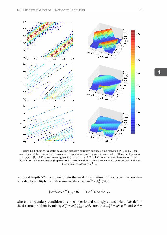
4.3. DISCRETISATION OF TRANSPORT PROBLEMS
4
67
Figure 4.8: Solutions for scalar advection diffusion equation on space-time manifold Q =Ω× [0,1] forn = 24, p = 2. Three cases were considered. Upper figures correspond to u,c,ε = 1,1,0, center figures to
u,c,ε = 1,1,0.001, and lower figures to u,c,ε = 1, 12 ,0.001. Left column shows iscontours of the
distribution as it travels through space-time. The right column shows surface plots. Colors/height indicatethe value of the density ρ(0))h .
temporal length ∆T = π/8. We obtain the weak formulation of the space-time problemon a slab by multiplying with some test-function w (0) ∈Λ(0)
0 (∆Q),
(w (0),LX ρ
(0))∆Q = 0, ∀w (0) ∈Λ(0)
0 (∆Q),
where the boundary condition at t = tk is enforced strongly at each slab. We definethe discrete problem by taking Λ(0)
h = S 2,2,224,24,8 ×S 2
8 , such that w (0)h = w Tφ(0) and ρ(0) =

4
68 4. SCALAR TRANSPORT
ρTφ(0). We find system of equations,
C(0,1)X E(1,0)ρ = 0.
The system needs to be solved slab-by-slab using the final solution at ∆Qk as initial so-lution for ∆Qk+1. Results are shown Figure 4.9a.
The shape and the height of the sinusoid are reasonably well preserved with someerror at its outer contour, and some deformation at its lower- and left side. Again, er-roneous wiggles are observed over the domain. These wiggles form a circular patternalong the sinusoids pathway. These oscillations generally have a large amplitude at theouter region where the transport velocity is the highest. In the next section we aim to geta better understanding of these oscillations, and try to control them.

4.3. DISCRETISATION OF TRANSPORT PROBLEMS
4
69
0.1 0.3 0.5 1.0x
0.1
0.3
0.5
1.0
y
0.10
0.05
0.00
0.05
0.10
0.20
0.30
0.40
0.50
0.60
0.70
0.80
0.90
1.00
1.10
(a) Reconstructed solution, ρ(0)h
0.1 0.3 0.5 1.0x
0.1
0.3
0.5
1.0
y
0.040
0.030
0.020
0.010
0.005
0.002
0.000
0.002
0.005
0.010
0.020
0.030
0.040
(b) Error, e(0)ρ
Figure 4.9: Contour plots of approximate solution ρ(0)h
and corresponding error e(0)ρ using a standard Galerkin
approach to solve the circular advection problem after one period, T =π. Spatial × temporal spline spaces
Λ(0)h
:=P2,224,24 ×S 2
8 , number of slabs k = 8.

4
70 4. SCALAR TRANSPORT
4.4. SUMMARY OF RESULTSThe Lie-derivative Lv describes variations of a k-form along the flow of some vectorfield v . It is related to the exterior derivative d and the interior product iv through Car-tan’s formula. The interior product iv describes the contraction of some k-form with avector field v , and it is a topological operator. These operators are used to construct acoordinate invariant representation of hyperbolic PDE’s.
The vector field v can be related to a 1-form v (1), which can be discretised in theexisting framework using nodal- and edge-type B-spline basis functions. This construc-tion introduces Hodge-? dependencies, inducing error in the discretisation, i.e. the ex-act structure of the interior product is not conserved. The contraction matrix Cv is theresulting inner product matrix of the interior product. The resulting system consists ofa linear combination of incidence, mass, and contraction matrices, E, M, and Cv . Thediscrete solution suffers from spurious oscillations, which grow over time.

5EULER EQUATIONS
The incompressible Euler equations in fluid dynamics describe balance of mass, mo-mentum, and energy in absence of viscosity and thermal conductivity when variationsof density are small, i.e. incompressible fluids. Solutions of these equations describe thepressure, velocity, thermal fields in a region of interest. The incompressible Euler equa-tions have a rich geometric structure, which studied in the classical work by Arnold, [15].The Euler equations contain various symmetries and invariants. In our discretisation weaim to preserve this structure, and conserve invariants in our simulations.
In section 5.1 we present an coordinate invariant representation of the Euler equa-tions, and discuss various formulations. The discretisation approach is discussed in sec-tion 5.2. The spatial discretisation can be constructed, such that the invariants are con-served at the semi-discrete level. The time integrator must be carefully selected to satisfythis conservation at each discrete time level. In section 5.3 we verify our results by run-ning various simulations.
5.1. THE EULER EQUATIONS
The Euler equations govern conservation of mass, momentum, and energy under theassumptions of incompressible and inviscid flow. Solutions of these equations describethe motion of idealised fluids. Under the assumption of incompressible flow, variationsin mass density ρ(n) are assumed to be small. For this case the mass and momentumequations can be solved independently from the energy equation. The assumption isgenerally used to model liquids and subsonic gas flows (i.e. low Mach number flows).Under the assumption of inviscid flow, viscous effects and shear stresses are assumed tobe zero. For this case, boundary layers and turbulent effects are neglected. This assump-tion is used to model convection-dominates flow (i.e. high Reynolds number flows) out-side boundary layers.
The conservation of momentum of an incompressible and inviscid fluid flow in Rn is
71

5
72 5. EULER EQUATIONS
given by,
∂v j
∂t+ vi
(∂v j
∂xi
)=− 1
ρ
∂p
∂x j+b j , (5.1)
with vi the components of the velocity field with j = 1, · · · ,n, p the pressure, ρ the massdensity, and bi components of body force. In Appendix I we derive a coordinate invariantform of the Euler equations expressed.
Theorem 5.1 (Euler Equations for Incompressible Flow, (Sec. 4.3c [18])). The equationsfor conservation of mass and momentum for an ideal incompressible fluid on manifoldM ⊂Rn are given by,
d∗v (1) = 0 (5.2)
∂v (1)
∂t+Lv v (1) =−d f (0), (5.3)
where v is the velocity-vector field, v (1) the velocity 1-form associated with v , and f (0)
given by,
f (0) =∫
d p
ρ− 1
2‖v (1)‖2 +φ(0),
with pressure p, mass density ρ, and potentialφ(0). We can solve for f (0) using the pressurePoisson equation, which can be obtained by taking the codifferetial d∗ of Equation I.3,and substitute the incompressibility constraint, Equation I.2,
d∗Lv v (1) =−∆ f (0). (5.4)
An equivalent system of equations can be derived by taking the exterior derivative d ofthese equations.
Theorem 5.2 (Vorticity Formulation of the Euler Equations). The equations for conser-vation of mass and momentum for an ideal incompressible fluid on manifold M ⊂Rn aregiven by,
∆ψ(2) =ω(2) (5.5)
∂ω(2)
∂t+Lvω
(2) = 0, (5.6)
where ψ(2) is the stream function with d∗ψ(2) = v (1), and vorticity ω(2) = d v (1).
The Euler equations have a Hamiltonian structure, which was studied in the classicalwork by Vladimir Arnold [15]. The equations govern various symmetries and invariants.In the discrete setting we aim to preserve these structures and conserve the mentionedquantities over time. The Euler equations satisfy conservation of integral circulation Γ,

5.1. THE EULER EQUATIONS
5
73
vorticity Ω, and helicity H ,
d
d tΓ= d
d t
∮γ(t )
v (1) = 0, (5.7)
d
d tΩ= d
d t
∫A(t )
ω(2) = 0, (5.8)
d
d tH = d
d t
∫V (t )
h(3) = 0, (5.9)
where h(3) = v (1)∧ω(2) is the helicity 3-form. Formal derivation of these results is given inAppendix I. Note that conservation of circulation and vorticity express an equal result,one can derive one from another by applying the generalised Stokes’ theorem, Equa-tion 2.13. Helicity is not the only quadratic invariant conserved by the Euler equations.The equations also govern conservation of kinetic-energy K ,
d
d tK = d
d t
1
2
(v (1), v (1))
V (t ) = 0, (5.10)
and in R2 the conservation of enstrophy S,
d
d tS = d
d t
1
2
(ω(2),ω(2))
V (t ) = 0. (5.11)
Proof of these relations is given in Appendix I.The exact part of the Lie derivative, i.e. div v (1), can be included in the right-hand-
side term to minimize the amount of terms that need to be discretised. We define theenergy head ,
g (0) := f (0) + iv v (1), (5.12)
such that the momentum equation, Equation I.3, can be written as,
∂v (1)
∂t+ iv d v (1) =−d g (0), (5.13)
which is known as Gromeka-Lamb’s formulation (sec. 4.4.10. [37]).We can obtain dual formulations of the Euler equations by applying the Hodge ?-
operator, and substituting the adjoint co-differential d∗ and co-Lie-derivative L ∗v , which
have been introduced in section 2.4 and section 4.1. In order to avoid confusion with v (1)
inR2 we denote q (1) = iv vol(n) as the (n−1)-form associated with the velocity vector fieldv .
Theorem 5.3 (Dual Formulations of the Euler equations). The dual equations for theconservation of mass and momentum for an ideal incompressible fluid on manifold M ⊂Rn are given by,
d q (n−1) = 0 (5.14)
∂q (n−1)
∂t− i∗vω
(n−2) = d∗g (n), (5.15)

5
74 5. EULER EQUATIONS
where v is the velocity-vector field, q (n−1) = ?v (1) the forms associated with v , ω(n−2) =(−1)n−1d∗q (n−1) is the dual vorticity form, and g (n) =?g (0) the energy head, Equation 5.12.The dual pressure Poisson equation is given by,
−di∗vω(n−2) =∆g (n). (5.16)
The stream function is given by ψ(n−2), such that dψ(n−2) = q (n−1). The dual vorticityformulation is given by,
(−1)n−1∆ψ(n−2) =ω(n−2) (5.17)
∂ω(n−2)
∂t−d∗i∗vω
(n−2) = 0. (5.18)
Note that d∗i∗vω(n−2) = i∗ω?q (1).
In the continuous setting primal and dual formulation are equivalent. In the discretesetting, however, as we have learned in the previous chapters, the choice of formulationhas an impact on the conservative properties. The exactness of the exterior derivative dcan be conserved. The primal formulation enables exactness of the vorticity constraintdd v (1) = dω(2) = 0 in the discrete setting, whereas the dual formulation enables exact-ness of the incompressibility constraint ddψ(n−2) = d q (n−1) = 0.
Note that the equations introduced need to be solved in pairs in order to solve for allunknowns. The pressure Poisson equation, Equation 5.16, needs to be solved togetherwith the momentum equations, Equation 5.15, to solve for unknowns q (1) and g (n). Sim-ilarly the stream function Poisson equation, Equation 5.17, needs to be solved with thevorticity equation, Equation 5.18, to solve for unknowns ω(n−2) and ψ(n−2). We will referto these as the momentum-pressure equations, and the vorticity-stream equations.
5.2. DISCRETISATION OF THE EULER EQUATIONSExactness of conservation of mass, i.e. the incompressibility constraint, is required inthe discrete setting in order to satisfy conservation of some other quantities as we willshow later on. This motivates us to discretise the dual formulations, where the incom-pressibility is governed by the exterior derivative d , rather than the codifferential d∗. Inthis section we will derive discretisations of the momentum and vorticity formulation.The semi-discrete system conserves integral mass, vorticity, kinetic energy and enstro-phy (proof in Appendix J). The time discretisation technique must carefully be selectedto conserve these quantities over time.
Definition 5.1 (discretisation of the Momentum-Pressure Formulation). Consider theperiodic unit square domain, Ω =]0,1[2. We obtain a weak-formulation of the pressurePoisson equation and the velocity equation, Equation 5.16 and Equation 5.15, by takingthe inner product with test functions r (2) ∈Λ(2)
0 (Ω) and s(1) ∈Λ(1)0 (Ω),(
r (2),di∗ω?q (1))Ω = (
r (2),dd∗g (2))Ω ,(
s(1),∂t q (1))Ω− (
s(1), i∗ω?q (1))Ω = (
d s(1), g (2))Ω
.

5.2. DISCRETISATION OF THE EULER EQUATIONS
5
75
Note that the pressure-Poisson equations needs to be solved by taking a system of firstorder equations as was done for the 2-form Poisson equation, Example 3.5. We definethe discrete solution by taking,
r (2)h = r Tφ(2), s(1)
h = sTφ(1),
g (2)h = g Tφ(2), q (1)
h = q Tφ(1),
which leads to the non-linear time-dependent system of equations,[−M(1,1)
(E(2,1)
)TM(2,2)
E(2,1) ;
][hg
]=
[0
−E(2,1)(M(1,1)
)−1C
(1,1)ωh
q
](5.19)
M(1,1) ∂q
∂t−C(1,1)
ωhq = (
E(2,1))TM(2,2)g . (5.20)
The semi-discrete system of non-linear equations satisfies conservation of mass, vortic-ity, kinetic energy, and enstrophy. Proof is presented in Appendix J. However, not everytime discretisation preserves the invariance of these quantities over time. Numericalschemes that preserve structures of Hamiltonian systems are symplectic integrators andenergy-conserving integrators. Palha and Gerritsma studied and derived these integra-tors for Hamiltonian ODE systems from a structure-preserving discretisation framework,[38]. The simplest of these methods is the implicit midpoint method.
Definition 5.2 (Implicit Midpoint Method). Given time-dependent system of non-linearequations,
d y(t )d t =A(y)y(t )
with, y(tk ) = y k ,(5.21)
where y k denotes the solution at time-instant tk . The implicit midpoint method is givenby,
y k+1 − y k
∆t=A(y)y , (5.22)
with y = 12
(y k+1 + y k
), and time-step ∆t = tk+1 − tk . The implicit midpoint method is
second order accurate in time.
Application of the implicit midpoint method to the discrete momentum equation,Equation J.2, yields the system of non-linear equations,
M(1,1) q k+1 −q k
∆t− 1
2C
(1,1)ωh
(q k+1 +q k
)= 1
2
(E(2,1))T
M(2,2) (g k+1 +g k
). (5.23)
We define the following algorithm,
1. Initialise:Given solution q k ,ωk , g k at time level tk . Let initially ω :=ωk .

5
76 5. EULER EQUATIONS
2. Iterate:Assemble contraction matrix C(1,1)
ωh. Simultaneously solve the discrete momentum
equation and the pressure-Poisson equation, Equation 5.23 and Equation J.1, toobtain solutions qk+1 and gk+1. Evaluate ωk+1, let ω := 1
2 (ωk+1 +ωk ). Iterate thisstep until set convergence criterion is met.
Conservation of mass depends on pairing of C(1,1)ωh
q and g , which can be achievedby simultaneously solving for qk+1 and gk+1. Conservation of integral vorticity is inde-pendent of the choice on time-integrator. It depends on the exactness of the exteriorderivative, which, by construction, is satisfied by E(1,0). Conservation of kinetic energyand enstrophy are preserved using the implicit midpoint method (can be checked us-ing the relations in Appendix J). However, enstrophy conservation depends on correctmatching of ω and q , which requires convergence of the linearisation technique. We letour convergence criterion depend on the enstrophy error, i.e. we iterate until
Sh(tk+1)−Sh(t0)
Sh(t0)≤ τ, (5.24)
where τ is the desired tolerance, e.g. τ= 10−6, and Sh the discrete enstrophy,
Sh =ωT (E(1,0))T
M(1,1)q . (5.25)
Definition 5.3 (discretisation of the Vorticity-Stream Formulation). Consider the peri-odic unit-square domain,Ω=]0,1[2. We obtain weak-formulations of the stream-functionPoisson equation and the vorticity equation, Equation 5.17 and Equation 5.18, by takingthe inner product with test functions r (0), s(0) ∈Λ(0)
0 (Ω),−(
dr (0),dψ(0))Ω = (
r (0),ω(0))Ω(
s(0),∂tω(0)
)Ω− (
iv d s(0),ω(0))Ω = 0
(5.26)
We define the discrete solution by taking,
r (0)h = r Tφ(0), s(0)
h = sTφ(0),
ψ(0)h =ψTφ(0), ω(0)
h =ωTφ(0),
which leads to the non-linear time-dependent system of equations,
M(0,0)ω+ (E(1,0))T
M(1,1)E(1,0)ψ= 0 (5.27)
M(0,0) ∂ω
∂t−
(C(0,1)
v hE(1,0)
)Tω= 0 (5.28)
We will prove that the discrete equations satisfy the relevant conservation laws that wederived in the previous section, section 5.1.

5.3. RESULTS, AND ANALYSIS
5
77
Application of the implicit midpoint method to the discrete vorticity equation, Equa-tion J.5, yields the system of non-linear equations,
M(0,0)ωk+1 −ωk
∆t− 1
2
(C
(0,1)v h
E(1,0))T
(ωk+1 +ωk ) = 0. (5.29)
We define the following algorithm.
1. Initialise:Given solution q k ,ωk , g k at time level tk . Let initially q := q k .
2. Iterate:Assemble contraction matrix C(0,1)
v h. Solve the discrete vorticity equation, Equa-
tion 5.29, to obtain ωk+1. Then solve the discrete stream-function Poisson equa-tion, Equation 5.27, to obtain solution stream-function ψk+1. Evaluate q k+1, andlet q := 1
2
(q k+1 +q k
). Iterate this step until set convergence criterion is met.
The advantage of this formulation is that conservation of mass is satisfied by con-struction of the stream-function. Therefore, it is not required to solve the vorticity- andPoisson equations simultaneously. Again, conservation of integral vorticity is indepen-dent on the choice of time integrator. Conservation of kinetic-energy and enstrophy arepreserved using the implicit midpoint method. However, conservation of kinetic-energydepends on the non-linear solution, and requires convergence of the linearisations tech-nique. We let the convergence criterion depend on the kinetic-energy error, i.e. we set,
Kh(tk+1)−Kh(t0)
Kh(t0)≤ τ, (5.30)
where τ is the desired tolerance, and Kh the discrete kinetic-energy,
Kh =ψTM(0,0)ω. (5.31)
It was shown by Palha and Gerritsma that the non-linear systems ,Equation 5.23 andEquation 5.29, can be combined into two systems of quasi-linear equations which can besolved staggered at time [17]. This approach combines the mass, vorticity, and enstrophyconserving properties of the vorticity formulation with the vorticity, and kinetic-energyconserving properties of the momentum formulation, and conserves all quantities with-out costly iterative techniques. In the next section we validate our results by introducingsome test problems.
5.3. RESULTS, AND ANALYSISThe problem of two co-rotating Taylor vortices was introduced by Mullen et al. to analyzethe performance of structure-preserving discretisations. Two equipotent vortices willsplit apart above some critical distance. Non-conserving methods fail to reproduce thisbehaviour after which the vortices merge together into one big vortex, [33]. We will lookat the problem of

5
78 5. EULER EQUATIONS
Example 5.1 (Taylor Vortices). Consider the Euler equations on Ω =]0,1[2. As initialcondition we consider a distribution of N = 2 Taylor vortices of equal strength, whichinduce vorticity,
ω(x) =2∑
i=1
Uσi
a
(2− (r − ri )2
a2
)exp
1
2
(1− (r (x)− r i )2
a2
), (5.32)
where U = 1 is the maximal tangential velocity, a = 0.075 the vortex strength, σi = ±1,the direction of rotation (positive for counter-clockwise), and (r (x)− r i )2 the squareddistance to the i -th core. We place initial cores near the center of the domain, (xi , yi ) =(0.4,0.5), (0.6,0.5), Equation 5.32. The cores will start to circle around the center. Thevortices deform in a stretching motion, which causes a tail to be formed at each vor-tex. The cores briefly touch, but the cores have gained too much momentum to merge.Instead they drift apart. Note that stabilized numerical techniques would induce mo-mentum loss, which could fail in capturing this behaviour.
We considered two configurations to show that the conservative properties are inde-pendent of discretisation parameters. In the first configuration we used a spline basis ofpolynomial order p = 1 with dimension n = 48, and used a time-step ∆t = 1/16. In thesecond configuration we let p = 2 and n = 64, and let ∆t = 1/32. The solutions at t = 1.5are shown in Figure 5.1. Both configurations were able to capture the non-merging mo-tion. The resulting distributions are roughly the same. However, the cores correspond-ing to the first configuration are less compact. We also observe more local extrema in thecentre region and in the tail regions. Finally, there is a difference in the core locations.
The vortex-stream formulation governs static conservation of mass, and dynamicconservation of vorticity, kinetic energy, and enstrophy. We compare the dynamicallyconserved quantities to their initial value, whereas the static quantity is evaluated ateach instant. Results of both configurations are shown in Figure 5.1. Both configurationsconserve enstrophy, vorticity, and mass with great precision. Kinetic energy is boundedwith relative error less than 1 percent. The quadratic quantities, i.e. kinetic energy andenstrophy, are better conserved by the second configuration.

5.3. RESULTS, AND ANALYSIS
5
79
0.0 0.5 1.0x
0.0
0.5
1.0
y
t= 2.0
0.0 0.5 1.0x
0.0
0.5
1.0
y
t= 2.0
50
40
25
10
6
0
2
20
30
45
Figure 5.1: Vorticity ω(0) at t = 1.5 of Taylor vortices on a periodic domain. Spline basis n = 48, p = 1, andtime-step ∆t = 1/32 (left), and n = 64, p = 2, ∆t = 1/64 (right).

5
80 5. EULER EQUATIONS
0.0 0.5 1.0x
0.0
0.5
1.0
y
t= 0.0
0.0 0.5 1.0x
0.0
0.5
1.0
y
t= 0.25
0.0 0.5 1.0x
0.0
0.5
1.0
y
t= 0.5
0.0 0.5 1.0x
0.0
0.5
1.0
y
t= 0.75
0.0 0.5 1.0x
0.0
0.5
1.0
y
t= 1.0
0.0 0.5 1.0x
0.0
0.5
1.0
y
t= 1.25
50
40
25
10
6
0
2
20
30
45
Figure 5.2: Vorticity ω(0) at various time-instants of simulated motion of an initial distribution of co-rotatingTaylor vortices on a periodic domain. Results were obtained using spline basis of polynomial order p = 2 and
dimension n = 64, and time-step size ∆t = 1/64.
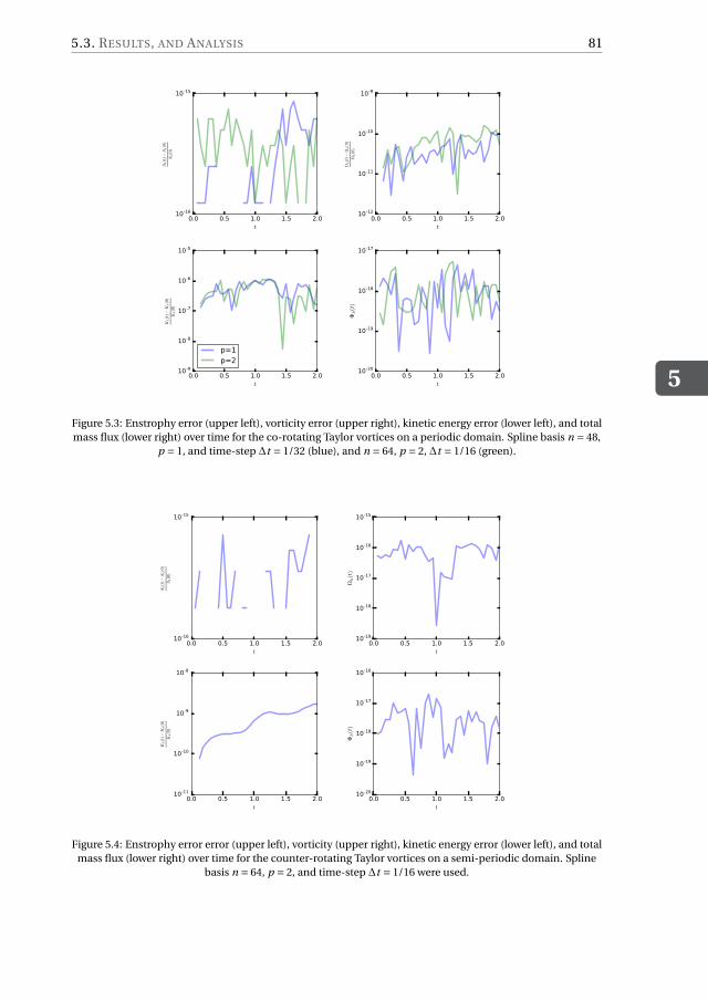
5.3. RESULTS, AND ANALYSIS
5
81
0.0 0.5 1.0 1.5 2.0t
10-16
10-15
Sh(t
)−Sh(0
)
Sh(0
)
0.0 0.5 1.0 1.5 2.0t
10-12
10-11
10-10
10-9
Ωh(t
)−
Ωh(0
)
Ωh(0
)
0.0 0.5 1.0 1.5 2.0t
10-9
10-8
10-7
10-6
10-5
Kh(t
)−Kh(0
)
Kh(0
)
p=1p=2
0.0 0.5 1.0 1.5 2.0t
10-20
10-19
10-18
10-17
Φh(t
)
Figure 5.3: Enstrophy error (upper left), vorticity error (upper right), kinetic energy error (lower left), and totalmass flux (lower right) over time for the co-rotating Taylor vortices on a periodic domain. Spline basis n = 48,
p = 1, and time-step ∆t = 1/32 (blue), and n = 64, p = 2, ∆t = 1/16 (green).
0.0 0.5 1.0 1.5 2.0t
10-16
10-15
Sh(t
)−Sh(0
)
Sh(0
)
0.0 0.5 1.0 1.5 2.0t
10-19
10-18
10-17
10-16
10-15
Ωh(t
)
0.0 0.5 1.0 1.5 2.0t
10-11
10-10
10-9
10-8
Kh(t
)−Kh(0
)
Kh(0
)
0.0 0.5 1.0 1.5 2.0t
10-20
10-19
10-18
10-17
10-16
Φh(t
)
Figure 5.4: Enstrophy error error (upper left), vorticity (upper right), kinetic energy error (lower left), and totalmass flux (lower right) over time for the counter-rotating Taylor vortices on a semi-periodic domain. Spline
basis n = 64, p = 2, and time-step ∆t = 1/16 were used.
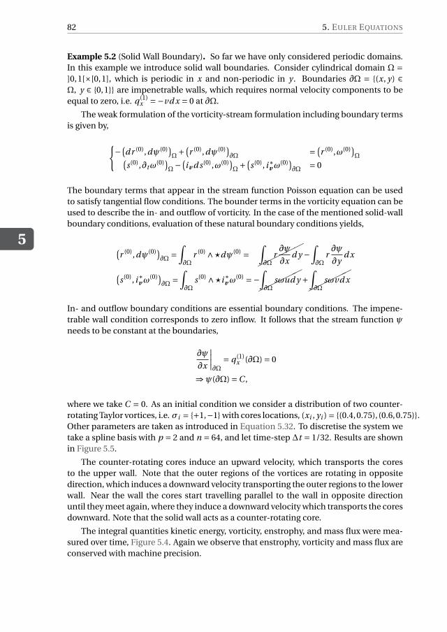
5
82 5. EULER EQUATIONS
Example 5.2 (Solid Wall Boundary). So far we have only considered periodic domains.In this example we introduce solid wall boundaries. Consider cylindrical domain Ω =]0,1[×[0,1], which is periodic in x and non-periodic in y . Boundaries ∂Ω = (x, y) ∈Ω, y ∈ 0,1 are impenetrable walls, which requires normal velocity components to beequal to zero, i.e. q (1)
x =−vd x = 0 at ∂Ω.
The weak formulation of the vorticity-stream formulation including boundary termsis given by,
−(
dr (0),dψ(0))Ω+ (
r (0),dψ(0))∂Ω = (
r (0),ω(0))Ω(
s(0),∂tω(0)
)Ω− (
iv d s(0),ω(0))Ω+ (
s(0), i∗vω(0))∂Ω = 0
The boundary terms that appear in the stream function Poisson equation can be usedto satisfy tangential flow conditions. The bounder terms in the vorticity equation can beused to describe the in- and outflow of vorticity. In the case of the mentioned solid-wallboundary conditions, evaluation of these natural boundary conditions yields,
(r (0),dψ(0))
∂Ω =∫∂Ω
r (0) ∧?dψ(0) =
∫∂Ω
r∂ψ
∂xd y −
∫∂Ω
r∂ψ
∂yd x
(s(0), i∗vω
(0))∂Ω =
∫∂Ω
s(0) ∧?i∗vω(0) =−
∫∂Ω
sωud y +
∫∂Ω
sωvd x
In- and outflow boundary conditions are essential boundary conditions. The impene-trable wall condition corresponds to zero inflow. It follows that the stream function ψ
needs to be constant at the boundaries,
∂ψ
∂x
∣∣∣∣∂Ω
= q (1)x (∂Ω) = 0
⇒ψ(∂Ω) =C ,
where we take C = 0. As an initial condition we consider a distribution of two counter-rotating Taylor vortices, i.e. σi = +1,−1 with cores locations, (xi , yi ) = (0.4,0.75), (0.6,0.75).Other parameters are taken as introduced in Equation 5.32. To discretise the system wetake a spline basis with p = 2 and n = 64, and let time-step ∆t = 1/32. Results are shownin Figure 5.5.
The counter-rotating cores induce an upward velocity, which transports the coresto the upper wall. Note that the outer regions of the vortices are rotating in oppositedirection, which induces a downward velocity transporting the outer regions to the lowerwall. Near the wall the cores start travelling parallel to the wall in opposite directionuntil they meet again, where they induce a downward velocity which transports the coresdownward. Note that the solid wall acts as a counter-rotating core.
The integral quantities kinetic energy, vorticity, enstrophy, and mass flux were mea-sured over time, Figure 5.4. Again we observe that enstrophy, vorticity and mass flux areconserved with machine precision.
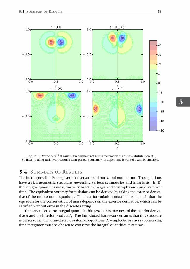
5.4. SUMMARY OF RESULTS
5
83
0.0 0.5 1.0x
0.0
0.5
1.0
y
t= 0.0
0.0 0.5 1.0x
0.0
0.5
1.0
y
t= 0.375
0.0 0.5 1.0x
0.0
0.5
1.0
y
t= 1.25
0.0 0.5 1.0x
0.0
0.5
1.0
y
t= 2.0
50
40
25
10
2
0
2
20
30
45
Figure 5.5: Vorticity ω(0) at various time-instants of simulated motion of an initial distribution ofcounter-rotating Taylor vortices on a semi-periodic domain with upper- and lower solid wall boundaries.
5.4. SUMMARY OF RESULTSThe incompressible Euler govern conservation of mass, and momentum. The equationshave a rich geometric structure, governing various symmetries and invariants. In R2
the integral quantities mass, vorticity, kinetic-energy, and enstrophy are conserved overtime. The equivalent vorticity formulation can be derived by taking the exterior deriva-tive of the momentum equations. The dual formulation must be taken, such that theequation for the conservation of mass depends on the exterior derivative, which can besatisfied without error in the discrete setting.
Conservation of the integral quantities hinges on the exactness of the exterior deriva-tive d and the interior product iv . The introduced framework ensures that this structureis preserved in the semi-discrete system of equations. A symplectic or energy conservingtime integrator must be chosen to conserve the integral quantities over time.


6CONCLUSION & FUTURE
DIRECTIONS
This thesis is the result of a research project on discretisation techniques for CFD. Theproject was divided in three objectives. The first objective was to study the existing exist-ing structure-preserving IGA framework for elliptic PDE’s. The second objective was toexpand this theoretical framework to discretise hyperbolic PDE’s, and the third objectivewas to construct a structure-preserving IGA discretisation for the incompressible Eulerequations, chapter 5.
Recently, some attention has been focused on structure-preserving discretisationtechniques within the scientific community. In these techniques special care is taken inthe preservation of fundamental mathematical structures, symmetries, and invariantsin the discretisation process. Exterior calculus proves to be insightful in identifying rel-evant topological dependencies. In exterior calculus we describe elliptic PDE’s with thetopological derivative operator d and the metric dual Hodge-? operator. Conservationof the important topological structure of the derivative operator d lies at the heart of thestructure-preserving framework. The framework is of theoretical relevance. It explainsthe correctness of using dual grids in finite-volume methods, and allows derivation ofinf-sub stable basis functions in finite-element methods.
The extension to hyperbolic PDE’s is not trivial. A superior theory to discretise theconvective terms and the vector fields is unavailable at this moment. However, by care-fully selecting the geometric formulation of the PDE, it is possible to conserve the nilpo-tency property of the interior product. This proved to be the key ingredient in the con-struction of an energy-conserving discretisation for the incompressible Euler equationsin R2. These discrete Euler equations behave as the continuous Euler equations whenthe mesh has sufficient resolution to represent relevant vortical structures, and whenspurious oscillations are within bounds. It needs to be verified if this construction isvalid for arbitrary geometries.
The next step is to develop a structure-preserving discretisation for the incompress-ible Euler equations in R3. It will be challenging to conserve integral helicity. Another
85

86 6. CONCLUSION & FUTURE DIRECTIONS
step might be the discretisation of the compressible Euler equations, for which there ex-ists a wide range of formulations and discretisaions. I wonder if it is possible to identifyan optimal formulation, or some fundamental construction, that needs to be satisfiedat the discrete level. These directions will improve our understanding of discretisationsand improve accuracy of simulations.
ADERHAM COHOMOLOGY
The DeRham sequence has important topological relations that governs existence of dif-ferential forms on manifolds. In cohomology we reduce these relations to topologicalstructures, i.e. chains and cochains. In section 2.3 we have shown that the codifferentialδ is the topological analogue of the exterior derivative d . In this chapter we introducethe structures corresponding to the exterior derivative d , the coboundary operator δ,and the codifferential d∗. We will present the Poincaré lemma and the Hodge decompo-sition.
Definition A.1 (Closed Forms, (Sec. 5.2 [18])).A k-form α(k) is closed if dα(k) = 0. The space of closed k-forms ZdΛ
(k) is the kernel ofthe exterior derivative, i.e.
ZdΛ(k) := α(k) ∈Λ(k) : dα(k) = 0 ⊂Λ(k).
Definition A.2 (Exact Forms, (Sec. 5.2 [18])).A k formα(k) is exact if there exists aβ(k−1) s.t. α(k) = dβ(k−1). The space of exact k-formsBdΛ
(k−1) is the range of the exterior derivative, i.e.
BdΛ(k−1) := dΛ(k−1) ⊂Λ(k).
It follows that every exact form is closed, i.e. if,
β(k−1) s.t. α(k) = dβ(k−1) then dα(k) = ddβ(k−1) = 0.
The topological structure is depicted in Figure A.1. The converse is true on contractiblemanifolds. Contractible spaces can be continuously reduced to a point. Examples in-clude any (star) domain in Euclidean space.
Theorem A.1 (Poincaré Lemma, (Sec. 5.4 [18])).On a contractible manifold M every closed k-form is exact, i.e.
∀α(k) ∈ZdΛ(k)(M ), there exists β(k−1) ∈Λ(k−1)(M ) s.t. α(k) = dβ(k−1).
87

A
88 A. DERHAM COHOMOLOGY
Λ(k−1) Λ(k)
ZdΛ(k)
HΛ(k)BdΛ(k−1)
Λ(k+1)
∅
d
d
Figure A.1: Poincaré Lemma, The range of the exterior derivative BdΛ(k−1) is contained in the kernel ZdΛ
(k).On contractible domains the converse is also true, for which then BdΛ
(k−1) =ZdΛ(k).
The theorem proofs existence of solutions for balancing relations is physics. Theserelations, often of the form grad(φ) = f , curl(~ω) = ~g , and div(~v) = h, are fundamental inphysics. From the theorem it also follows that for any volume form α(n), there exist apotential function. Since dΛ(n) = 0, we have thatΛ(n) =ZdΛ
(n), hence
∀α(n) ∈Λ(n) =ZdΛ(n), ∃β(n−1) ∈BdΛ
(k−1) s.t. dβ(n−1) =α(n). (A.1)
Thus the exterior derivative acting on Λ(n−1) is surjective on contractible domains(surjectivity of the ∇· operator). Note that this is only true if and only if the boundaryconditions satisfy the compatibility condition. Finally, the theorem implies that the ker-nel of Λ(k) is equal to dΛ(k−1) on contractible manifolds, i.e. BdΛ
(k−1) =ZdΛ(k). Hence
we can decompose the space of k-formsΛ(k) into
Λ(k)(M ) =ZdΛ(k) ⊕Z C
d Λ(k), (A.2)
where Z Cd denotes the complement of ZdΛ
(k) in Λ(k). On non-contractible domainswe can define the space of k-forms which are closed but not exact. We call such formsHarmonic forms.
Definition A.3 (Harmonic forms, (Sec. 14.2 [18])). The space of harmonic k-forms HΛ(k)
is defines as
HΛ(k) := α(k) ∈ZdΛ(k) :α(k) 6∈BdΛ
(k−1).
On contractible domains HΛ(k) =;. The space of closed k-forms can be written as thesum of exact k-forms united with the space of harmonic k-forms,
ZdΛ(k) =BdΛ
(k−1) ⊕HΛ(k).
If we combine this expression with Equation A.2 we obtain,
Λ(k)(M ) =BdΛ(k−1) ⊕HΛ(k) ⊕Z C
d Λ(k).
This result is known as the Hodge decomposition. The Hodge decomposition enables usto decompose differential forms in algebraic complements.

A
89
Definition A.4 (Co-closed Forms, (Sec. 14.2 [18])).A k-form α(k) is co-closed if d∗α(k) = 0. The space of co-closed k-forms Zd∗Λ(k) is thekernel of the codifferential, i.e.
Zd∗Λ(k) := α(k) ∈Λ(k) : d∗α(k) = 0 ⊂Λ(k).
Definition A.5 (Co-exact Forms, (Sec. 14.2 [18])).A k form α(k) is co-exact if ∃β(k+1) s.t. α(k) = d∗β(k+1). The space of co-closed k-formsBd∗Λ(k+1) is the range of the codifferential, i.e.
Bd∗Λ(k+1) := d∗Λ(k+1) ⊂Λ(k)
Definition A.6 (Harmonic Form, (Sec. 14.2 [18])).In line with our previous definition, section 2.2, we can define the space of harmonicforms as follows,
HΛ(k) := α(k) ∈ZdΛ(k) :α(k) 6∈BdΛ
(k−1)
HΛ(k) := α(k) ∈Zd∗Λ(k) :α(k) 6∈Bd∗Λ(k+1).
These definitions can be united as follows. A k-form α(k) is harmonic if ∆α(k) = 0. Thespace of harmonic k-forms is defined as,
HΛ(k) := α(k) ∈Λ(k) : dα(k) = d∗α(k) = 0.
As in section 2.2 we can decompose the space of k-forms in orthogonal components,
Λ(k)(M ) =BdΛ(k−1) ⊕HΛ(k) ⊕Z C
d Λ(k)
Λ(k)(M ) =Bd∗Λ(k+1) ⊕HΛ(k) ⊕Z Cd∗Λ
(k).
The decompositions can be unified by taking Z Cd Λ(k) =Bd∗Λ(k+1) and Z C
d∗Λ(k) =BdΛ
(k−1).This leads to a more useful definition of the Hodge decomposition.
Theorem A.2 (Hodge decomposition, (Sec. 14.2 [18])).For any k-form on a closed manifold M there exists an unique decomposition
α(k) = dφ(k−1) +d∗ψ(k+1) +h(k),
where h(k) is a harmonic form. Note that this doesn’t imply uniqueness of φ(k−1) andψ(k+1). On a contractable manifold the space of harmonic forms is empty, i.e. h(k) = 0.
The coboundary operator δ induces the same topological structure on cochain com-plexes. We can define cochain spaces analogue to the spaces of closed-, exact-, and har-monic form.
BδC (k−1) := δC (k−1),
ZδC (k) := c (k) ∈C (k) : δc (k) =;,
HC (k) := c (k) ∈ ZδC (k) : c (k) 6∈ BδC (k−1),
The topological structure of these spaces is shown in equivalent to the one shown inFigure A.1. The topology of the exterior derivative is preserved in discrete cochain struc-tures. This structure governs discrete counterparts of the Poincaré lemma, that dependson the exactness of the coboundary operator.
BDERIVATION OF ADJOINT
RELATIONS
In section 2.4 we introduced the L2-inner product through the action of the Hodge-?operator. In this chapter we derive the various adjoint relations that have been usedthroughout the work. Let L :Λ(k)(M ) →Λ(l )(M ) be a linear operator. The adjoint oper-ator is the liner operator L ∗ :Λ(l )(M ) →Λ(k)(M ) that satisfies,(
α(k),L ∗β(l ))M
=(Lα(k),β(l )
)M
, (B.1)
for some α(k) ∈Λ(k)(M ) and β(l ) ∈Λ(l )(M ). The exterior derivative d , the interior prod-uct iv , and the Lie derivative Lv do not depend on metric. Their respective adjoints, thecodifferential d∗, the cointerior product i∗v , and the co-Lie derivative L ∗
v do explicitlydepend on the metric-dependent Hodge-? operator. The adjoint relations can be usedto obtain a more favourable weak formulation. Note that in many derivations we use thefollowing property of the Hodge-? operator, ??α(k) = (−1)k(n−k).
1. The codifferential:
d∗α(k) = (−1)n(k−1)+1?d ?α(k) (B.2)
Let α(k−1) ∈Λ(k−1), and β(k) ∈Λ(k), now
d(α(k−1) ∧?β(k)) =dα(k−1) ∧?β(k) + (−1)k−1α(k−1) ∧d ?β(k)
=dα(k−1) ∧?β(k) + (−1)k−1α(k−1) ∧((−1)(n−k+1)(k−1)??
)d ?β(k)
=dα(k−1) ∧?β(k) + (−1)(n−k)(k−1)α(k−1) ∧??d ?β(k)
=dα(k−1) ∧?β(k) + (−1)(n−k)(k−1)α(k−1) ∧?((−1)n(k−1)−1d∗
)β(k)
=dα(k−1) ∧?β(k) + (−1)−k(k−1)−1α(k−1) ∧?d∗β(k)
=dα(k−1) ∧?β(k) −α(k−1) ∧?d∗β(k).
90

B
91
In the last line we used that k(k − 1) is even for all k. By rearranging the terms,integrating over manifold M , and using Theorem 2.2 and Definition 2.15, we find,∫
Mα(k−1) ∧?d∗β(k) =
∫M
dα(k−1) ∧?β(k) −∫∂M
α(k−1) ∧?β(k)
⇔(α(k−1),d∗β(k)
)M
=(dα(k−1),β(k)
)M
−∫∂M
α(k−1) ∧?β(k). (B.3)
The adjoint relation is obtained when the boundary term reduces to zero.
2. The cointerior product:
i∗v := (−1)n(k+1)−1? iv? (B.4)
Let α(k) ∈Λ(k), β(k−1) ∈Λ(k−1), and v be a vector field, and v (1) the 1-form associ-ated with v . Substitution the 1-form isomorphism, Equation 4.10, in the definitionof i∗v yields,
i∗vβ(k−1) =(−1)nk−1+(k−1)(n−k+1)??(??β(k−1) ∧ v (1))
=(−1)nk−1+(k−1)(n−k+1)+(k−1)(n−k+1)+k(n−k)(β(k−1) ∧ v (1))
=(−1)k2−1(β(k−1) ∧ v (1))
=(−1)k−1(β(k−1) ∧ v (1)),
Taking the inner product of β(k−1) and ivα(k) yields,(
β(k−1), ivα(k)
)M
=∫Mβ(k−1) ∧?ivα
(k)
4.10= (−1)k(n−k)∫Mβ(k−1) ∧??
(?α(k) ∧ v (1)
)=(−1)k(n−k)+(n−k+1)(k−1)
∫Mβ(k−1) ∧?α(k) ∧ v (1)
=(−1)k(n−k)+(n−k+1)(k−1)+(n−k)∫Mβ(k−1) ∧ v (1) ∧?α(k)
=(−1)k−1(β(k−1) ∧ v (1),α(k)
)M
=(i∗vβ
(k−1),α(k))M
The cointerior product i∗v is the adjoint of the interior product iv .(β(k−1), ivα
(k))M
=(i∗vβ
(k−1),α(k))M
(B.5)
3. The co-Lie derivative:
L ∗v := (−1)k(n+1)+1?Lv ? . (B.6)

B
92 B. DERIVATION OF ADJOINT RELATIONS
The co-Lie derivative is related to the codifferential and cointerior product that issimilar Cartan’s formula, Equation 4.5. Let α(k) ∈Λ(k) and v some vector field. Wefind,
L ∗v α
(k) 4.5= (−1)k(n+1)+1? (div ?+? iv d)?α(k)
=(−1)k(n+1)+1?((−1)(n−k−1)(k+1)d ??iv + (−1)(n−k+1)(k−1)? iv ??d
)?α(k)
=(−1)k(n+1)+1((−1)(n−k−1)(k+1)+nd∗i∗v + (−1)(n−k+1)(k−1)+n i∗v d∗
)α(k)
=(d∗i∗v + i∗v d∗)α(k). (B.7)
Using adjoint relations Equation B.3 and Equation B.5 we find,(β(k),L ∗
v α(k)
)M
B.7=(β(k),d∗i∗vα
(k))M
+(β(k), i∗v d∗α(k)
)M
=(dβ(k), i∗vα
(k))M
−(β(k), i∗vα
(k))∂M
+(ivβ
(k),d∗α(k))M
=(iv dβ(k),α(k)
)M
−(β(k), i∗vα
(k))∂M
(B.8)
+(divβ
(k),α(k))M
−(ivβ
(k),α(k))∂M
4.5=(Lvβ
(k),α(k))M
−(β(k), i∗vα
(k))∂M
−(ivβ
(k),α(k))∂M
. (B.9)
The adjoint relation is obtained when the boundary terms reduce to zero.

CGENERALISED PIOLA
TRANSFORMATIONS
In this chapter we derive the pull-back operators for k-forms in R3. These transforma-tions commutate with the exterior derivative, such that the DeRham structure is pre-served on arbitrary geometries. Note that these transformations are also useful whendetermining integrals on some parent domain.
Definition C.1 (Pull-back operator φ∗, (Sec. 2.7 [18])).Consider smooth bijective coordinate mapping φ : N →M . Consider local coordinatesxi for manifold M and ξ j for manifold N , such that x = φ(ξ) = x(ξ). Let α(0) ∈Λ(0)(M )be some 0-form. We define pull-back operator φ∗ to be equal to (φ∗α(0))(ξ) := α(x(ξ)).The pull-back operator satisfies the following properties,
φ∗(dα(0)) = d(φ∗α(0))
φ∗(α(k) ∧β(l )) = (φ∗α(k))∧ (φ∗β(l ))
We can use these properties to derive pull-back operators for arbitrary k-forms inR3. Letβ(1) be some 1-form.
φ∗β(1) =φ∗(βi d xi ) =βi (x(ξ))dφ∗(xi )
=βi (x(ξ))∂xi
∂ξ jdξ j
= βdξ j = β(1).
or β=βF , where F = Fi j = ∂xi
∂ξ j is the deformation gradient. Now for some 2-formω(2) we
93

C
94 C. GENERALISED PIOLA TRANSFORMATIONS
find,
φ∗ω(2) =φ∗ωi j d xi ∧d x j =ωi j (x(ξ))(φ∗d xi )∧ (φ∗d x j )
=ωi j (x(ξ))∂xi
∂ξk
∂x j
∂ξldξk ∧dξl
= ω(2),
with i 6= j , and k 6= l . We find that ∂xi
∂ξk∂x j
ξl dξk ∧dξl defines the adjugate of the deforma-
tion gradient matrix, i.e.
ω=ωAdj(F ) =ω(detF )(F−1).
Note that this relations is famous as the Piola (stress) transformation. Finally, for some3-form ρ(3) we find,
φ∗ρ(3) = ρ(x(ξ))∂xi
∂ξl
∂x j
∂ξm
∂xk
∂ξn dξl ∧dξm ∧dξn ,
where we obtain ρ = ρ(detF ). These transformations for the components of k-formscommute with the exterior derivative, such that any DeRham complex in some physicalspace is also satisfied in some pull-backed parameter space. The transformations areknown as the generalized Piola transformations. We can pull-back integrals using thegeneral pull-back formula.
Theorem C.1 (General pull-back formula, (Sec. 3.1 [18])).Consider again the smooth bijective coordinate mapping φ : N → M . Let U ⊂ N , such
that φ(U ) ⊂ M . Let α(k) ∈ Λ(k)(M ) be a k-form. The integral of α(k) on φ(U ) can bepulled-back to U , ∫
φ(U )α(k) =
∫Uφ∗α(k). (C.1)

DWELL-POSEDNESS OF THE
POISSON PROBLEM
Well-posedness of elliptic PDE problems can be analysed in the powerful Hilbert spacesetting. In this setting, weak formulations of the PDE problems are analysed. We willintroduce some fundamental properties and theorems that enable us to prove existenceand uniqueness to the PDE problems. Furthermore we prove well-posedness for thePoisson problems that were introduced in chapter 3.
Lemma D.1 (Cauchy-Schwarz inequality).Any two k-forms α(k),β(k) ∈ L2Λ(k) satisfy the inequality
|(α(k),β(k))| ≤ ‖α(k)‖L2Λ(k)‖β(k)‖L2Λ(k) (D.1)
Lemma D.2 (Generalised Poincaré inequality, (proof in [39])).Consider a k-form α(k) ∈ WdΛ
(k)(Ω) on contractible manifold Ω, i.e. the space of har-monic k-forms is empty. Then α(k) satisfies,
‖α(k)‖L2Λ(k) ≤C‖dα(k)‖L2Λ(k+1) , (D.2)
for some constant C . The Poincaré inequality allows us to define an equivalent Sobolevnorm ‖α(k)‖WdΛ
k := ‖dαk‖L2Λ(k+1) .
Definition D.1 (Weakly coercive).Let H1, H2 denote Hilbert spaces. A bilinear form B(·, ·) : H1×H2 →R is weakly coercive if
supv∈H2
B(u, v)
‖v‖H2
≥α‖u‖H1 , ∀u ∈ H1,
and supu∈H1
B(u, v)
‖u‖H1
≥α‖v‖H2 , ∀v ∈ H2,
where α ∈R.
95

D
96 D. WELL-POSEDNESS OF THE POISSON PROBLEM
Definition D.2 (Coercive).A bilinear form B(·, ·) : H ×H →R is coercive if
B(u,u) ≥α‖u‖2H , ∀u ∈ H .
Definition D.3 (Continuous).A bilinear form B(·, ·) : H1 ×H2 →R is continuous if
|B(u, v)| ≤ c‖u‖H1‖v‖H2 ,
where c ∈R.
The Lax-Milgram theorem is a powerful theorem to prove existence and uniquenessof solution to coercive PDE problems. We will also consider indefinite variational prob-lems for which well-posedness can be proved using Brezzi’s theorem, Theorem D.4.
Theorem D.3 (Lax-Milgram).Let u, v ∈ H, and let F : H →R define a bounded linear functional, and let a(·, ·) : H×H →R be a continuous, coercive, bilinear form. Then
∃!u ∈ H s.t. a(u, v) = F (v), ∀v ∈ H .
Problem D.1 (Mixed Variational Problem).Given a pair of Hilbert spaces H1,H2, bilinear forms a(·, ·) : H1×H1 →R, b(·, ·) : H1×H2 →R, and bounded linear functionals F (·) : H1 →R, and G(·) : H2 →R. We then seek u ∈ H1,p ∈ H2 s.t.
a(u, v)−b(v, p) = F (v),
b(u, q) =G(q),(D.3)
∀v ∈ H1, ∀q ∈ H2.
Theorem D.4 (Inf-Sup Condition - Brezzi’s Theorem (Sec. 2.1 [22])).Let Z = v ∈ H1 : b(v, q) = 0, ∀q ∈ H2, let bilinear form a(·, ·) be continuous on H1 × H1
and coercive on Z ×Z . There exists an unique solution (u, p) ∈ H1 ×H2 for Problem D.1 ifand only if bilinear form b(·, ·) is continuous on H1 ×H2 and if
supv∈H1
b(v, p)
‖v‖H1
≥C‖p‖H2 .
We will apply these theorems to two example problems in the framework of exteriorcalculus using the DeRham Sobolev Complex. The first problem, the 0-form Poissonproblem, is associated with unconstrained optimization of a quadratic functional. Thistype of problem has classically been solved successfully using Rayleigh-Ritz approach. Inthis approach the problem is converted to a set of discrete minimization problems withresulting linear problemAu = f , whereA is a symmetric positive definite (SPD) matrix.

D
97
Example D.1 (0-form Poisson problem).Consider the domain Ω = [0,1]2 ⊂ R2 with boundary ∂Ω = Γd ∪Γn , where Γd ∩Γn = ;.
Given f (0) ∈Λ(0), find ψ(0) ∈Λ(0) such that,∆ψ(0) = f (0),
ψ(0) = 0, on Γd
∂nψ(0) = 0, on Γn
We obtain a weak formulation of this problem by taking the inner product with some testfunction w (0) ∈Λ(0)
0 . WhereΛ(0)0 is the space of compactly supported 0-forms according,
Λ(0)0 := α(0) ∈Λ(0) : tr α(0) = 0 on Γd .
We use integration by parts for two reasons. First, we would like to reduced the conti-nuity constraints on the considered trial space. Secondly, we would like to get rid of thecodifferential d∗. We find,(
w (0),d∗dψ(0))Ω = (
w (0), f (0))Ω
⇔ (d w (0),dψ(0))
Ω = (w (0), f (0))
Ω+ (w (0),dψ(0))∂Ω.
For this case the boundary integral reduces to zero. We hence obtain the following weakformulation. Given f (0) ∈ L2Λ(0), find ψ(0) ∈WdΛ
(0) s.t.(d w (0),dψ(0))
Ω = (w (0), f (0))
Ω , ∀w (0) ∈WdΛ(0)0 .
We can rewrite this problem in variational formulation, defining bilinear form a(·, ·) andfunctional F (·),
a(·, ·) : WdΛ(0) ×WdΛ
(0) →R : a(·, ·) := (d ·,d ·)ΩF (·) : WdΛ
(0) →R : F (·) := (·, f (0))Ω.
Given ψ(0) ∈ L2Λ(0), find ψ(0) ∈WdΛ(0) such that,
a(w (0),ψ(0)) = F (w (0)), ∀w (0) ∈Λ(0)0 .
Lax-Milgram proves existence of unique solution if a(·, ·) is coercive, and continuous,and F (·) is bounded. Using Cauchy-Schwarz (CS), and Poincaré (PC), we find
|a(w (0),ψ(0))| = (d w (0),dψ(0))ΩC S≤ ‖d w (0)‖‖dψ(0)‖ <∞,
a(w (0), w (0)) = (d w (0),d w (0))Ω = ‖d w (0)‖2 PC≥ C‖w (0)‖2,
‖F‖ = sup‖w (0)‖≤1
|F (w (0))| C S≤ sup‖w (0)‖≤1
‖w (0)‖‖ f (0)‖ = ‖ f (0)‖ <∞.
Note that we used the boundedness of norms that exists by definitions of function spacesL2Λ(0) and WdΛ
(0). Hence by Lax-Milgram there exists an unique solution ψ(0) ∈WdΛ(0)
s.t. a(w (0),ψ(0)) = F (w (0)), ∀w (0) ∈W 0dΛ
(0).

D
98 D. WELL-POSEDNESS OF THE POISSON PROBLEM
In the second problem we will consider the volume, n-form, Poisson problem. Thisproblem is equivalent to constrained optimization of a quadratic functional. These prob-lems are solved numerically using a mixed Galerkin formulation.
Example D.2 (n-form Poisson problem, (Sec. 2.3 [23])).Consider the domain Ω = [0,1]2 ⊂ R2 with boundary ∂Ω = Γd ∪Γn , where Γd ∩Γn = ;.
Given f (2) ∈Λ(2), find ψ(2) ∈Λ(2) such that,∆ψ(2) = f (2), inΩ,
ψ(2) = 0, on Γd ,
∂tψ(2) = 0, on Γn
Again we multiply with some test-function w (2) and perform integration by parts forreasons mentioned before to obtain,(
d∗w (2),d∗ψ(2))Ω = (
w (2), f (2))Ω .
We could use a similar roadmap as for the 0-form Poisson case, using Lax-Milgram toprove well-posedness, and taking the dual Sobolev space Wd∗Λ(2). However, in the finiteprojection method, we will only be able to satisfy one of the DeRham Sobolov complexessimultaneously. Hence we want to limit ourselves to the use of the following sequenceof function spaces in proving well-posedness of the problem.
WdΛ(0) WdΛ
(1) L2Λ(2)d d
Consider the equivalent system of first-order-differential equations,d∗ψ(2) = v (1),
d v (1) = f (2)
A weak formulation can be obtained taking inner product with q (1) ∈ WdΛ(1)0 and w (2) ∈
L2Λ(2) respectively, and performing integration by parts, where
Λ(1)0 := α(1) ∈Λ(1) : tr α(1) = 0 on Γn.
We obtain,(d q (1),ψ(2)
)Ω+ (
q (1),ψ(2))∂Ω = (
q (1), v (1))Ω , ∀q (1) ∈WdΛ
(1)0 ,(
w (2),d v (1))Ω = (
w (2), f (2))Ω , ∀w (2) ∈ L2Λ(2).
Note that the boundary integral reduces to zero due to the induced boundary conditions.We can define bilinear forms a(·, ·), and b(·, ·) and functional F (·),
a(·, ·) :Λ(2) ×Λ(2) →R : a(·, ·) := (·, ·)Ωb(·, ·) : WdΛ
(1) ×L2Λ(1) →R : b(·, ·) := (d ·, ·)ΩF (·) : WdΛ
(0) →R : F (·) := (·, f (0))Ω.

D
99
Now we can rewrite the problem in the variational formulation. Given f (2) ∈ L2Λ(2), findψ(2) ∈ L2Λ(2) and v (1) ∈WdΛ
(1) such that,a(q (1), v (1))−b(q (1),ψ(2)) = 0, ∀q (1) ∈Λ(1)
0
b(v (1), w (2)) = F (w (2)), ∀w (2) ∈Λ(2).
Let ZdΛ(1) = q (1) ∈WdΛ
(1) : d q (1) = 0. Note that the exterior derivative on (n−1)-formsis surjective, Equation A.1, which implies that for any ψ(2) ∈ L2Λ(2), there exists someq (1)ψ ∈WdΛ
(1), such that ψ(2) = d q (1)ψ , and ‖ψ(2)‖ = ‖d q (1)
ψ ‖.Brezzi’s theorem, Theorem D.4, can now be used to prove well-posedness of this
problem. We need to prove that a(·, ·) is coercive on ZdΛ(1) ×ZdΛ
(1), that b(·, ·) is con-tinuous, and that the inf-sup condition is satisfied for b(·, ·).
a(q (1), q (1)) = ‖q (1)‖2WdΛ
(1) = ‖q (1)‖L2Λ(1) +‖d q (1)‖L2Λ(2) ,
|b(q (1),ψ(2))| = |(d q (1),ψ(2))| C S≤ ‖d q (1)‖‖ψ(2)‖ <∞
supq (1)∈WdΛ
(1)
b(q (1),ψ(2))
‖q (1)‖ ≥b(q (1)
ψ ,ψ(2))
‖q (1)ψ ‖
= ‖ψ(2)‖2
‖q (1)ψ ‖
≥ 1
C‖ψ(2)‖,
where we used that ‖q (1)ψ ‖ PC≤ C‖d q (1)
ψ ‖ =C‖ψ(2)‖. Hence there exists an unique solution
set (v (1),ψ(2)) ∈ (WdΛ(1),L2Λ(2)). Note that well-posedness depended on the exact se-
quence that is satisfied by the Sobolev DeRham complex. In our discretization approachwe must ensure that our finite-dimensional function spaces satisfy the exact sequenceto prove well-posedness in the discrete setting. In the 0-form Poisson example this wasnot the case which poses less restrictions on the choice of finite-dimensional functionspaces in the discretization process.

EDERIVATION OF EDGE FUNCTIONS
The finite-dimensional function spaces are constructed by taking spans of combinationsof nodal- and edge-type basis functions as is shown in section 3.3. In this chapter wederive the edge-type basis function and prove its unit mass property.
Consider the 1-form v (1)h ∈ L2Λ(1)
h that satisfies v (1)h = d f (0)
h . The question is, how do
we define L2Λ(1)h ? Do we let L2Λ(1)
h := Sp
n as well? Application of the exterior derivative
on the 0-form f (0)h yields the following,
d f (0)h (ξ) =
(d
dξ
n∑i=1
λi ,p (ξ) fi
)dξ
3.17=(
n∑i=1
(p
ξi+p −ξiλi ,p−1(ξ)− p
ξi+p+1 −ξi+1λi+1,p−1(ξ)
)fi
)dξ
=
p
ξp −ξ0λ1,p−1(ξ)dξ · f1 − p
ξp+1 −ξ1λ2,p−1(ξ)dξ · f1
+ p
ξp+1 −ξ1λ2,p−1(ξ)dξ · f2 −·· · · · ·
· · · · · ·− p
ξn+p −ξnλn,p−1(ξ)dξ · fn−1
+ p
ξn+p −ξnλn,p−1(ξ)dξ · fn −
((((((((
((((((p
ξn+p+1 −ξn+1λn+1,p−1(ξ)dξ · fn
=n∑
i=2
(p
ξi+p −ξiλi ,p−1(ξ)dξ
)( fi − fi−1)
Where we used that ξp − ξ0 = ξn+p+1 − ξn+1 = 0. If we let vi = ( fi − fi−1), and use B-spline basis functions of a polynomial degree lower with scaling p
ξi+p−ξi, then the relation
v (1)h = d f (0)
h is exact.
100
E
101
Unit mass. Take v (1)h = d f (0)
h with,
fi =
C , if i < j
C +1, if i ≥ j,
for some constant C ∈R, such that vi = δ ji . Now,
∫ ξ j+p
ξ j
λ(1)j (ξ)dξ=
∫ ξ j+p
ξ j
(n∑
i=2λ(1)
i (ξ)vi
)dξ
=∫ ξ j+p
ξ j
v (1)h =
∫ ξ j+p
ξ j
d f (0)h dξ= f (0)
h
∣∣∣ξ j+p
ξ j= (C +1)−C = 1
This property reduces integration of 1-forms to mere summation of the expansioncoefficients, i.e. for some v (1)
h ∈ L2,
∫Ω
v (1)h =
∫Ω
(n∑
i=2λ(1)
i (ξ)vi
)dξ=
n∑i=2
vi

FCONSTRUCTION OF BOUNDED
COCHAIN PROJECTIONS
We want to construct projection operators, Π(k), that commute with the exterior deriva-tive conform,
Λ(k) Λ(k+1)
C (k) C (k+1)
d
δ
Π(k+1)Π(k)
Such commuting projection operators are known as cochain projection operators. Boundedcochain operators are fundamental in analysis. These projection operators allow us toprovide estimates of the discrete solution with respect to the continuous solution. Moreon bounded cochain projectors can be found in the work by Falk and Winter, [5, 40].Construction of such operators is not trivial, standard Galerkin L2 projections of a k-form and k+1-form do not yield the desired commutativity. However, one can constructsuch projection by introducing a Poisson problem. An example is given in Appendix F.
Example F.1 (Construction of bounded cochain projections for ω(2) = d v (1) in R2).Consider the pair v (1) ∈WdΛ
(1) and ω(2) ∈ L2Λ(2) onΩ= [0,1]2 given by,
v (1) =− 1
4πcos(2πx)sin(2πy)d x − 1
4πsin(2πx)cos(2πy)d y
ω(2) = d v (1) = sin(2πx)sin(2πy)d x ∧d y.
We want to define bounded projection operators satisfying commutativity δΠ(1)v (1) =Π(2)d v (1). We let WdΛ
(1) := S 2,37,8 ×S 3,2
8,7 and L2Λ(2) := S 2,27,7 . To define Π(2) we consider
102

F
103
standard L2 projection, i.e.
(s(2)
h ,ω(2)h
)Ω=
(s(2)
h ,ω(2))Ω
, ∀s(2)h ∈ L2Λ(2)
h ,
Using the existence of q (1), such that, s(2) = d q (1), Equation A.1, and using ω(2) = d v (1),we find an equivalent formulation,
(d q (1)
h ,d v (1)h
)Ω=
(d q (1)
h ,d v (1))Ω
, ∀q (1)h ∈WdΛ
(1)h .
Integration by parts yields,
(∆q (1)
h , v (1)h
)Ω−
(d q (1)
h , v (1)h
)∂Ω
=(∆q (1)
h ,d v (1))Ω−
(d q (1)
h , v (1))∂Ω
, q (1)h ∈WdΛ
(1)h .
Hence we let,
Π(2) : L2Λ(2) →C (2), ω(2) Π(2)
→ ω(2)h with,
(s(2)
h ,ω(2)h
)Ω=
(s(2)
h ,ω(2))Ω
, ∀s(2)h ∈ L2Λ(2)
h
Π(1) : WdΛ(1) →C (1), v (1) Π
(1)
→ v (1)h with,
(∆q (1)
h , v (1)h
)Ω=
(∆q (1)
h , v (1))Ω
, ∀q (1)h ∈WdΛ
(1)h
To reduce continuity constraints, conform the chosen space WdΛ(1), we will work we the
integrated-by-parts version ofΠ(1). We obtain systems of equations,
M(2,2)ω= (φ(2),ω(2))
Ω(E(2,1))T
M(2,2)E(2,1)v − (E(2,1))T
(φ(2), v (1)
h
)∂Ω
= (E(2,1))T (
φ(2),d v (1))Ω− (
E(2,1))T (φ(2), v (1))
∂Ω .
A reconstruction of δΠ(1)v (1) is shown in Figure F.1. We find,
‖δΠ(1)v (1) −Π(2)d v (1)‖L2 = 1.2469e −15,
with,
‖v‖2L2 :=
dim(v )∑i
|vi |2.

F
104 F. CONSTRUCTION OF BOUNDED COCHAIN PROJECTIONS
x
0.0
0.2
0.4
0.6
0.8
1.0
y
0.0
0.2
0.4
0.6
0.8
1.0
ω(2
)h
1.0
0.5
0.0
0.5
1.0
Figure F.1: Reconstruction of bounded cochain projection δΠ(1)v (1).

GDERIVATION OF TRANSPORT
PROBLEMS
We can derive the integral transport equations by analysing how some k-formα(k) pairedto some k-dimensional sub-manifold V ⊂M evolves as it is advected with some velocityvector field v . Let φt be the flow associated with v , such that V (t ) =φt V . Theorem 4.1.From Theorem C.1 it follows that,∫
V (t )α(k) =
∫Vφ∗
t α(k). (G.1)
We can derive the transport theorem by differentiating this relation with respect to tyields,
d
d t
∫V (t )
α(k)(t ) = lim∆t→0
1
∆t
(∫V (t+∆t )
α(k)(t +∆t )−∫
V (t )α(k)(t )
)= lim∆t→0
1
∆t
(∫V (t+∆t )
α(k)(t +∆t )−∫
V (t+∆t )α(k)(t )
+∫
V (t+∆t )α(k)(t )−
∫V (t )
α(k)(t )
)G .1= lim
∆t→0
1
∆t
(∫Vφ∗
t+∆t [α(k)(t +∆t )−α(k)(t )]+∫
V[φ∗
t+∆t −φ∗t ]α(k)(t )
)=
∫Vφ∗
t lim∆t→0
α(k)(t +∆t )−−α(k)(t )
∆t+
∫Vφ∗
t lim∆t→0
φ∗∆t −1
∆tα(k)(t )
4.3=∫
Vφ∗
t∂α(k)
∂t+
∫Vφ∗
t Lvα(k)
=∫
V (t )
(∂α(k)
∂t+Lvα
(k)
).
105

G
106 G. DERIVATION OF TRANSPORT PROBLEMS
The time-rate of change of a k-formα(k) ∈Λ(k) paired to a k-dimensional sub-manifoldV ⊂M at some time-instant t ∈R is thus given by,
d
d t
∫V (t )
α(k) =∫
V (t )
(∂α(k)
∂t+Lvα
(k)
). (G.2)
Example G.1 (Conservation of mass, incompressible flow, and the advection-diffusionequation).Consider a volume V (t ) ⊂M ⊂Rn filled with some quantity with mass density ρ(n). Thequantity’s mass is given by,
M =∫
V (t )ρ(n).
Conservation of mass implies dd t M = 0. Applying Theorem 4.2 yields,
0 = d
d tM = d
d t
∫V (t )
ρ(n) =∫
V (t )
(∂ρ(n)
∂t+Lvρ
(n))
, (G.3)
Using Cartan’s formula and the fact that dρ(n) = 0, we find that Lvρ(n) = divρ
(n). We canre-express the volume-form, ρ(n) = ρ vol(n). Now,
divρ(n) = divρ vol(n) = dρiv vol(n) 4.14= dρv (n−1) = d q (n−1),
where q (n−1) := ρv (n−1) is the mass flux. Hence,∫V (t )
∂ρ(n)
∂t=−
∫V (t )
d q (n−1) =−∫∂V (t )
q (n−1), (G.4)
i.e. the time-rate of change of mass in the volume is balanced by the flux of the materialthrough the volume’s boundary. Additionally, we may want to take into account diffusivefluxes. Diffusive fluxes satisfy some constitutive law of the form,
q (n−1)diffusive =−εd∗ρ(3),
where the material parameter ε > 0 is the rate of diffusion. Examples of these consti-tutive laws are discussed in section 2.5. The total flux is then equal to the sum of theadvective flux and the diffusive flux, q (n−1) = ivρ
(3) − εd∗ρ(3). Substituting this relationinto Equation G.4 yields, ∫
V (t )
∂ρ(n)
∂t=−
∫V (t )
d(iv −εd∗)ρ(3)
⇔∫
V (t )
(∂ρ(n)
∂t+Lvρ
(n) −ε∆ρ(n))= 0,
where we assumed ε to be constant. The result is known as the scalar advection-diffusionequation. Note that in the case of convection, when ρ(3) is the mass density of the flowitself, there cannot be an additional diffusive term. In that case all information governing

G
107
the flow of the material is contained in its velocity v . In the case of a convection problem,conservation of mass is governed by,∫
V (t )
(∂ρ(n)
∂t+Lvρ
(n))= 0. (G.5)
Under the assumption of incompressible flow, variations of mass density ρ(n) are negli-gible within the volume V (t ), i.e. derivatives of ρ are assumed to be zero. For this casewe find that,
0 =∫
V (t )
(∂ρ(n)
∂t+Lvρ
(n)
)
=∫
V (t )dρv (n−1)
=∫
V (t )ρd v (n−1).
Hence an incompressible smooth flow in V (t ) satisfies d v (n−1) = 0. We will refer to thiscondition as the incompressibility constraint. Note that by the Poincaré lemma, Theo-rem 2.1, there exists some potential function ψ(n−2), such that dψ(n−2) = v (n−1). Thispotential function is known as the stream function.
Example G.2 (Stream function ψ(n−2)).We can retrieve the path of a fluid parcel by determining iso-surfaces of the stream func-tion. Consider some fluid parcel with mass density ρ(n) that is advected along some flowwith velocity field v on M . Along its path we find that,
Lvφtρ(n) 4.3= d
d t[φ∗
t φtρ(n)] = d
d t
[ρ(n)∣∣
t=0
]= 0.
Hence it follows that divρ(n) = d q (n−1) = 0. By the Poincaré lemma, Theorem 2.1, there
exists a potential function ψ(n−2), such that dψ(n−2) = q (n−1). Note that the stream func-tion satisfies the equation iv dψ(n−2) = iv q (n−1) = iv ivρ
(n) = 0.Now consider the case of incompressible flow, for which the there exists a stream
function ψ(n−2), such that dψ(n−2) = v (n−1). Hence,
Lvρ(n) = d(ρ(0) ∧ v (n−1))
= dρ(0) ∧ v (n−1) +
ρ(0) ∧d v (n−1)
= dρ(0) ∧dψ(n−2)
Let γ be a (n − 1)-dimensional iso-contour of the stream function ψ(n−2), i.e. a sub-manifold on which ψ(n−2) equals some constant. Satisfying the conservation of mass,Equation G.5, along this iso-contour yields,
0 = ∂ρ(n)
∂t+Lvρ
(n) = ∂ρ(n)
∂t+(((((
((dρ(0) ∧dψ(n−2), ∀x ∈ γ.

G
108 G. DERIVATION OF TRANSPORT PROBLEMS
Hence the fluid parcel remains constant along γ, and γ is its path. If the flow field istime dependent, then iso-contours are streaklines. Now let A be the (n−1)-dimensionalsurface that is bounded by various iso-contours of ψ(n−2), e.g. as shown in Figure G.1.Then the integral flux through A is constant,∫
Aq (n−1) =
∫A
dψ(n−2) =∫∂Aψ(n−2) =C .
A
C1
C4
C2
C3
Figure G.1: Surface A (red) bounded by iso-surfaces (blue) of the stream function ψ(1) = C1,C2,C3,C4. Theintegral flux is constant for any area bounded by the iso-surfaces,
∫A q(2) = ∫
∂A ψ(1) =C1 −C2 −C3 +C4.
From the principle of conservation of mass of some quantity with mass density ρ(n)
that is transported along some incompressible flow with velocity field v we can formu-late 4 equivalent formulations,
∂ρ(n)
∂t+Lvρ
(n) = 0, (G.6)
∂ρ(n)
∂t−L ∗
v ρ(n) = 0, (G.7)
∂ρ(0)
∂t+Lvρ
(0) = 0, (G.8)
∂ρ(0)
∂t−L ∗
v ρ(0) = 0, (G.9)
where ρ(n) = ρ vol(n) = ρ(0) ∧ vol(n) or ρ(0) = ?ρ(n). Equation G.6 and Equation G.9 areknown as conservative formulations of the conservation of mass, whereas Equation G.7and Equation G.8, are known as non-conservative formulations.
Proof. Equation G.6 follows from the integral conservation of mass, Equation G.5, underthe assumption of smoothness within V (t ). We can derive Equation G.9 by taking theHodge-? of Equation G.6,
?Lvρ(n) =?Lv ?ρ
(0) 4.19= −L ∗v ρ
(0).

G
109
The same strategy can be used to derive Equation G.7 from Equation G.8. Equivalenceof Equation G.6 and Equation G.8 can be shown by comparing Lvρ
(n) with ?Lvρ(0),
Lvρ(n) = div (ρ(0) ∧vol(n)) = d(ρ(0) ∧ v (n−1)) = dρ(0) ∧ v (n−1) +
ρ(0) ∧d v (n−1),
?Lvρ(0) =?iv dρ(0) =?? (?dρ(0) ∧ v (1)) = dρ(0) ∧?v (1) = dρ(0) ∧ v (n−1),
where we used the assumption of incompressible flow, d v (n−1) = 0. And hence it followsthat Lvρ
(n) =?Lvρ(0).

HCONSTRUCTION OF PERIODIC
BASIS
In this chapter we show how the periodic basis of Figure 4.5 can be constructed from anordinary B-spline basis through knot insertion on the domain Ω = [0,1]. The periodicbasis can be seen as an interior part of an extended ordinary B-spline basis, Figure H.1.Through knot insertion we can lower the continuity of the basis at ∂Ω, such that the in-terior part becomes an ordinary basis. From the knot insertion algorithm, Definition 3.6,we obtain the mapping Tp : T
pn → S
pn+2(p−1). This mapping can be manipulated such
that it links the basis functions crossing ∂Ω.Consider the B-spline shown in top of Figure H.1 with dimension n = 8 polynomial
order p = 2, and knot vector,
Ξ= 1
4−1,−1,−1,0,1,2,3,4,5,5,5.
To obtain C 0 at ∂Ω, we insert the knots 0,1. From Definition 3.6 we obtain the linearmap to the new n = 10 dimensional basis,
T=
1 0 0 0 0 0 0 00 1 0 0 0 0 0 00 1
212 0 0 0 0 0
0 0 1 0 0 0 0 00 0 0 1 0 0 0 00 0 0 0 1 0 0 00 0 0 0 0 1 0 00 0 0 0 0 1
212 0
0 0 0 0 0 0 1 00 0 0 0 0 0 0 1
We delete the first- and last p = 2 rows and (p −1 = 1) columns corresponding to basis
110

H
111
functions supported outside the domainΩ,
T=
12
12 0 0 0 0
0 1 0 0 0 00 0 1 0 0 00 0 0 1 0 00 0 0 0 1 00 0 0 0 1
212
The first- and final (p = 2) basis functions cross the boundary ∂Ω. The (p = 2)nd basisfunction can be linked to the final (n+p = 6)th basis function, and the (p −1 = 1)st basisfunction can be linked to the (n + p − 1 = 5)th basis function. Hence we add the 5thcolumn to the 1st, and the 6th to the 2nd,
T=
12
12 0 0
0 1 0 00 0 1 00 0 0 11 0 0 012
12 0 0
Hence we have obtained the map T : P 24 :→ S 2
6 . The reverse mapping that maps theordinary basis to the periodic equals the transpose TT : S 2
6 →P 24 , hence,
(Ti j )Tλi ,p =λpdj ,p ⇔ TTλp =λpd
p
We can use T to map mass matrices on periodic domains,
Mpd =(λ
pdp ,λpd
p
)Ω
=∫Ωλ
pdp ∧?λpd
p
=∫Ω
(TTλp
)∧?(TTλp
)=TT
(∫Ωλp ∧?λp
)T
=TTMT.
This enables us to use the normal assembly routines to construct mass matrices on pe-riodic domains.

H
112 H. CONSTRUCTION OF PERIODIC BASIS
0.00 0.25 0.50 0.75 1.00ξ
0.0
0.5
1.0
λ(0
) (ξ)
0.00 0.25 0.50 0.75 1.00ξ
0.0
0.5
1.0
λ(0
) (ξ)
Figure H.1: The periodic basis can be constructed by taking the inner part of an extended basis (top) andlinking the functions crossing the boundary ofΩ= [0,1]. Through knot insertion we can obtain a second basis
(bottom) whose inner part is an ordinary B-spline basis onΩ.

IDERIVATION OF THE EULER
EQUATIONS AND INVARIANTS
In Euler equations express conservation of mass, momentum, and energy in fluid dy-namics. In Appendix G, we derived an invariant formulation for the conservation of massusing the transport theorem, Theorem 4.2. In this section we will derive and analyse themomentum equations. In incompressible flow, i.e. variations in mass density ρ(n) areassumed to be small, we can solve the mass and momentum equation without solvingthe energy equation. The conservation of momentum under the assumption of a perfectfluid (viscous effects and shear stresses are assumed to be zero) and incompressible flowin Rn is given by,
∂v j
∂t+ vi
(∂v j
∂xi
)=− 1
ρ
∂p
∂x j+b j , (I.1)
with vi the components of the velocity field with j = 1, · · · ,n, p the pressure, ρ the massdensity, and bi components of body force.
To transform to invariant formulation we consider the momentum 1-form, P (1). Themomentum 1-form associates mass density with velocity along a line, dual to the massflux q (n−1) = ivρ
(n). We define,
P (1) = ρv (1) = ρ? v (n−1) =?ρiv vol(n) =?ivρ(n) =?q (n−1),
with v (1) = vi d xi . The Lie-derivative of this velocity 1-form is given by,
Lv v (1) = (div + iv d) v (1)
=d v2i + iv
∂vi
∂x jd x j ∧d xi
=2vi∂vi
∂x jd x j + vi
∂v j
∂xid x j − vi
∂vi
∂x jd x j
=vi∂v j
∂xid x j + 1
2
∂v2i
∂x jd x j ,
113

I
114 I. DERIVATION OF THE EULER EQUATIONS AND INVARIANTS
and so,
∂v (1)
∂t+Lv v (1) =
(∂v j
∂t+ vi
∂v j
∂xi+ 1
2
∂v2i
∂x j
)d x j ,
which contains the terms on the right-hand-side of Equation I.1 plus an additionaal termcontaining the kinetic energy 1
2 v2i = 1
2 iv v (1) = 12‖v (1)‖2. Pressure and density are related
through a constitutive equation or an equation of state, p = p(ρ). Let G(ρ) := ∫ d pρ =
1ρ
d pdρ dρ, then
dG(ρ) = ∂G(ρ)
∂x jd x j =G ′(ρ)
∂ρ
x jd x j = 1
ρ
d p
dρ
∂ρ
∂x jd x j = 1
ρ
∂p
∂x jd x j .
Finally we assume the body force b(1) is uniform, e.g. gravity, such that db(1) = 0. Thenthere exists a potential function φ(0), Theorem 2.1, such that −dφ(0) = b(1). Now bymatching components with Equation I.1 we find the invariant form of the equations forconservation of momentum,
∂v (1)
∂t+Lv v (1) − 1
2‖v (1)‖2 =−d
(φ(0) +
∫d p
ρ
).
Note that this formulation of the momentum equations is known asIn Example G.1 we derived that conservation of mass for an incompressible fluid can
be expressed as d v (n−1) = 0, or d∗v (1) = 0. Note that for this case there exists a potentialfunction, the stream function ψ(n−2) or ψ(2), such that dψ(n−2) = v (n−1) or d∗ψ(2) = v (1).
Theorem I.1 (Euler Equations for Incompressible Flow, (Sec. 4.3c [18])). The equationsfor conservation of mass and momentum for an ideal incompressible fluid on manifoldM ⊂Rn are given by,
d∗v (1) = 0 (I.2)
∂v (1)
∂t+Lv v (1) =−d f (0), (I.3)
where v is the velocity-vector field, v (1) the velocity 1-form associated with v , and f (0),
f (0) =∫
d p
ρ− 1
2‖v (1)‖2 +φ(0),
with pressure p, mass density ρ, and potentialφ(0). We can solve for f (0) using the pressurePoisson equation, which can be obtained by taking the codifferetial d∗ of Equation I.3,and substitute the incompressibility constraint, Equation I.2,
d∗Lv v (1) =−∆ f (0). (I.4)
Next we introduce the vorticity 2-form ω(2), which is a measure of rotation withinthe flow. We derive an equation for the vorticity by taking the exterior derivative d ofequation Equation I.1,
d
(∂v (1)
∂t+Lv v (1)
)= ∂ω(2)
∂t+Lvω
(2) =−dd f (0) = 0.
I
115
From the incompressibility constraint we know that there exists a stream function suchthat v (1) = d∗ψ(2). We find,
ω(2) = d v (1) = dd∗ψ(2) =∆ψ(2).
Vorticity and the stream function are related through a Poisson equation.
Example I.1 (Conservation of circulation). We can pair Equation I.3 with some curveγ(t ) ⊂M , ∫
γ(t )
∂v (1)
∂t+Lv v (1) =−
∫γ(t )
d f (0) =−∫∂γ(t )
f (0).
We define circulation Γ := ∫γ(t ) v (1). Using the transport theorem, Theorem 4.2, we find,
d
d tΓ= d
d t
∫γ(t )
v (1) =−∫∂γ(t )
f (0). (I.5)
Hence along any closed curve γ(t ) the circulation Γ is constant in time. This result isknown as Kelvin’s circulation theorem.
Example I.2 (Conservation of Vorticity). We can pair Equation 5.6 with some surfaceA(t ) ⊂M and use the transport theorem Theorem 4.2 to find,
d
d t
∫A(t )
ω(2) = 0,
i.e. the integral vorticity within a surface is conserved over time. This result is simply are-exprssion of Kelvin’s theorem for conservation of circulation, Equation I.5,
d
d t
∫A(t )
ω(2) = d
d t
∫A(t )
d v (1) = d
d t
∫∂A(t )
v (1) = 0, (I.6)
with ∂A(t ) = γ(t ) the closed curve that bounds a surface. Note that we can Equation 5.6as,
LXω(2) = 0,
with X = ∂∂t + v the space-time velocity field. Hence vorticity is invariant under the flow
related to X .
Example I.3 (Conservation of Helicity). Finally we consider the helicity 3-form h(3) :=v (1) ∧ω(2). From the properties of the Lie-derivative,Definition 4.1, we find that,
LX h(3) =LX(v (1) ∧ω(2))=LX v (1) ∧ω(2) + v (1) ∧LXω
(2) =−d f (0) ∧ω(2) +v (1) ∧0.
Now,
d(
f (0) ∧ω(2))= d(
f (0) ∧d v (1))= d f (0) ∧d v (1) +
f (0) ∧dd v (1) = d f (0) ∧ω(2).

I
116 I. DERIVATION OF THE EULER EQUATIONS AND INVARIANTS
Again by applying the transport theorem after pairing helicity with some volume V (t ) ⊂M , we find
d
d t
∫V (t )
h(3) =∫
V (t )LX h(3) =−
∫V (t )
d(
f (0) ∧ω(2))=−∫∂V (t )
f (0) ∧ω(2) = 0, (I.7)
i.e. the integral helicity is conserved over time.
Example I.4 (Conservation of Kinetic Energy). The weak formulation is valid for anytest-function w (1), taking w (1) := v (1), we obtain an equation for the evolution of kineticenergy, (
v (1),∂t v (1))M + (
v (1),Lv v (1))M =−(
v (1),d f (0))M , (I.8)
where(v (1),∂t v (1)
)M = 1
2∂t(v (1), v (1)
)M = 1
2∂t‖v (1)‖2, i.e. the time-rate-of-change of thekinetic energy. We can substitute this identity and integrate by parts to obtain,
1
2
∂
∂t‖v (1)‖2+(((((
((((d∗v (1), iv v (1))
M +((((((((((
v (1) ∧ v (1),d v (1))M
=− (v (1), iv v (1))
∂M −
(
d∗v (1), f (0))M − (
v (1), f (0))∂M .
By properties of the wedge product we find v (1)∧v (1) =−v (1)∧v (1), such that v (1)∧v (1) =0. Furthermore d∗v (1) = 0 for incompressible flow, and so we obtain,
1
2
∂
∂t‖v (1)‖2 =−(
v (1), iv v (1) + f (0))∂M .
It follows that the integral amount of kinetic energy within the domain is balanced bysome boundary flux-term, and hence conserved within boundary-less domains. A simi-lar result by deriving a weak formulation of the dual formulation.
We obtain a weak formulation of the primal vorticity formulation of the momen-tum equation, Equation 5.6, by taking the inner product with some test function s(2) ∈Λ(2)(M ), and obtain, (
s(2),∂tω(2))
M + (s(2),divω
(2))M = 0 (I.9)
Example I.5 (Conservation of Enstrophy ‖ω(2)‖2 in R2). We take s(2) :=ω(2) in weak for-mulation, Equation I.9, to obtain an equation for the evolution enstrophy,
1
2
∂
∂t‖ω(2)‖2 + (
ω(2),Lvω(2))
M = 0, (I.10)
where(ω(2),∂tω
(2))M = 1
2∂t(ω(2),ω(2)
)M = 1
2∂t‖ω(2)‖2, i.e. the time-rate-of-change of
enstrophy. In M ⊂R2 vorticity ω(2) =ω(0) ∧vol(2) =ωvol(2) is a scalar field, and hence,(ω(2),Lvω
(2))M = 1
2
∫M
d‖ω‖2q (1) =∫∂M
‖ω‖2q (1), (I.11)
where q (1) is the velocity (n−1)-form associated with the vector field v . In R2 we use v (1)
and q (1) to distinguish between the various 1-forms that are associated with v . It followsthat the enstrophy is balanced by some boundary flux-term. Note that this result is onlyvalid in R2. In R3 vortex stretching leads to very different mechanics.

JPROOF DISCRETE EULER
EQUATIONS SATISFY
CONSERVATION LAWS
In this chapter we prove that the semi-discrete equations introduced in section 5.2 sat-isfy conservation of integral mass, vorticity, kinetic-energy, and enstrophy at each timeinstant. Consider the vorticity-stream formulation,
[−M(1,1)
(E(2,1)
)TM(2,2)
E(2,1) ;
][hg
]=
[0
−E(2,1)(M(1,1)
)−1C
(1,1)ωh
q
](J.1)
M(1,1) ∂q
∂t−C(1,1)
ωhq = (
E(2,1))TM(2,2)g . (J.2)
1. Conservation of Mass:We obtain an equation for the evolution of the divergence of the velocity field by
pre-multiplying the discrete momentum equation, Equation J.2, with E(2,1)(M(1,1)
)−1,
E(2,1) ∂q
∂t−(((((
(((((
E(2,1) (M(1,1))−1C(1,1)ωh
q =(((
(((((((
(((
E(2,1) (M(1,1))−1 (E(2,1))T
M(2,2)g ,
with the two terms cancel out by Equation J.1.
2. Conservation of Vorticity:Vorticity and velocity are related through ω(0)
h = d∗q (1)h , or
M(0,0)ω= (E(1,0))T
M(1,1)q .
117

J
118 J. PROOF DISCRETE EULER EQUATIONS SATISFY CONSERVATION LAWS
The integral vorticity is then given by,∫Ωω(0)
h dΩ=(1,ω(0)
h
)Ω= 1TM(0,0)ω=(((((
(((1T (
E(1,0))TM(1,1)q = 0,
where again E(1,0)1 = 0. This is the discrete version of Kelvin’s circulation theorem.
3. Conservation of Kinetic Energy:We define the error e(1)
q = q (1) −q (1)h with, q (1)
h = q Tφ(1). We find,
0 = 1
2
∂
∂t‖q (1)‖2 =
(q (1)
h +e(1)q ,∂t q (1)
h +∂t e(1)q
)Ω
= 1
2
∂
∂t
(‖q (1)
h ‖2 +‖e(1)q ‖2
)+
(q (1)
h ,∂t e(1)q
)Ω+
(e(1)
q ,∂t q (1)h
)Ω
1
2
∂
∂t
(‖q (1)
h ‖2 +‖e(1)q ‖2
).
It follows that the discrete kinetic energy, 12‖q (1)
h ‖2 is balanced by the error’s kineticenergy. Hence by constructing a scheme that conserves the discrete kinetic energy,we consistently approximate the continuous kinetic energy, and bound the growthof the error’s kinetic energy. Th evolution of the discrete kinetic energy is given by,
1
2
d
d t
∫Ω
q (1)h ∧?q (1)
h =(q (1)
h ,∂t q (1)h
)Ω= q TM(1,1) ∂q
∂t.
Hence by pre-multiplying Equation J.2 with q T we obtain an equation for the evo-lution of the discrete kinetic energy,
q TM(1,1) ∂q
∂t−q TC(1,1)
ωhω=(((((
(((q T (
E(2,1))TM(2,2)g , (J.3)
with the right-hand-side term reduces to zero by conservation of mass, E(2,1)q = 0,and,
q TC(1,1)ωh
ω=(q (1)
h , i∗ωh?q (1)
h
)Ω=
(q (1)
h , i∗v hω(0)
h
)Ω
=(iv h q (1)
h ,ω(0)h
)Ω=
(iv h iv h vol(2),ω(0)
h
)Ω= 0.
We find that the conservation of kinetic-energy depends on the nilpotency of theinterior product.
4. Conservation of Enstrophy:We obtain an equation for the evolution of enstrophy by taking the test functionequal to the derivative of the vorticity,
1
2
d
d t
∫Ωω(0)
h ∧?ω(0)h =
(ω(0)
h ,∂tω(0)h
)Ω=
(ω(0)
h ,∂t d∗q (1)h
)Ω
=(dω(0)
h ,∂t q (1)h
)Ω=ωT (
E(1,0))TM(1,1) ∂q
∂t.

J
119
Hence, pre-multiplication of the discrete momentum equation, Equation J.2, with(E(1,0)ω
)Tyields,
ωT (E(1,0))T
M(1,1) ∂q
∂t−(((((
(((ωT (
E(1,0))TC(1,1)ωh
q =((((
(((((((
(ωT (
E(1,0))T (E(2,1))T
M(2,2)g ,
where the right-hand-side term equals zero due to the exterior derivative’s nilpo-tency. For the other term we find,
ωT (E(1,0))T
C(1,1)ωh
q =(dω(0)
h , i∗v hω(0)
h
)Ω=
(iv h dω(0)
h ,ω(0)h
)Ω
J .6= 0.
Next consider the velocity-pressure formulation,
M(0,0)ω+ (E(1,0))T
M(1,1)E(1,0)ψ= 0 (J.4)
M(0,0) ∂ω
∂t−
(C(0,1)
v hE(1,0)
)Tω= 0 (J.5)
1. Conservation of Mass:Conservation of mass is trivial with q = E(1,0)ψ, such that E(2,1)q = 0 with machineprecision.
2. Conservation of Vorticity:We obtain an equation of the evolution of the integral vorticity by by taking theunit test-function, 1 = 1Tφ(0),
d
d t
∫Ωω(0)
h dΩ=(1,∂tω
(0)h
)Ω= 1TM(0,0) ∂ω
∂t.
Hence, pre-multiplying the discrete vorticity equation, Equation J.5, with the unit-vector 1 yields,
1TM(0,0) ∂ω
∂t−
1T(C(0,1)
v hE(1,0)
)Tω= 0,
where E(1,0)1 = 0 trivially. So the discrete conservation of vorticity is satisfied throughthe exterior derivative.
3. Conservation of Kinetic Energy:We obtain an equation of the evolution of the integral kinetic energy by taking thetest-function equal to the stream function,
1
2
d
d t‖q (1)
h ‖2 =(q (1)
h ,∂t q (1)h
)Ω=
(dψ(0)
h ,∂t q (1)h
)Ω=
(ψ(0)
h ,∂tω(0)h
)Ω=ψTM(0,0) ∂ω
∂t.
Pre-multiplication of Equation J.5 withψ yields,
ψTM(0,0) ∂ω
∂t−
ψT(C(0,1)
v hE(1,0)
)Tω= 0,

J
120 J. PROOF DISCRETE EULER EQUATIONS SATISFY CONSERVATION LAWS
where,
ψT(C(0,1)
v hE(1,0)
)Tω= q T
(C(0,1)
v h
)Tω=
(iv h q (1)
h ,ω(0))Ω= (
iv h iv h vol(2),ω(0))Ω = 0.
Conservation of kinetic energy depends on the nilpotency of the interior product,which in this case is exactly satisfied due to the construction of q (1)
h = iv h vol(2).
4. Conservation of Enstrophy:Next we’ll analyze the enstrophy. We define error e(0)
ω =ω(0) −ω(0)h , and find,
0 = 1
2
∂
∂t‖ω(0)‖2 =1
2
∂
∂t
(ω(0)
h +e(0)ω ,∂tω
(0)h +∂t e(0)
ω
)Ω
=1
2
∂
∂t
(‖ω(0)
h ‖2 +‖e(0)ω ‖2
)+
(ω(0)
h ,∂t e(0)ω
)Ω+
(e(0)ω ,∂tω
(0)h
)Ω
=1
2
∂
∂t
(‖ω(0)
h ‖2 +‖e(0)ω ‖2
)It follows that the discrete enstrophy, 1
2‖ω(0)h ‖2, is balanced by the error’s enstro-
phy. Hence the error’s enstrophy is bounded if we can construct a scheme thatconserves the discrete enstrophy. Furthermore, the generalized Poincaré inequal-ity, Equation D.2, states,
‖q (1)h ‖2 D.2≤ C 2‖d∗q (1)
h ‖2 =C 2‖ω(0)h ‖2.
The discrete kinetic energy is bounded by the discrete enstrophy.
To obtain an equation for the evolution of enstrophy we take test function equalto the vorticity, ω(0)
h =ωTφ(0),
1
2
d
d t
∫Ωω(0)
h ∧?ω(0)h =
(ω(0)
h ,∂tω(0)h
)Ω=ωTM(0,0) ∂ω
∂t.
Hence, pre-multiplication of the discrete vorticity equation, Equation J.5, with thevorticity vectorω yields,
ωTM(0,0) ∂ω
∂t−
ωT(C(0,1)
v hE(1,0)
)Tω= 0,
where,
ωT(C(0,1)
v hE(1,0)
)Tω=
(iv h dω(0)
h ,ω(0)h
)Ω
I .11= 1
2
∫Ω
d‖ω(0)h ‖2q (1)
h = 1
2
∫∂Ω
‖ω(0)h ‖2q (1)
h = 0.
(J.6)
Hence conservation of enstrophy depends on the incompressibility constraint,and on the exactness of the exterior derivative.

KPICARD AND NEWTON
LINEARISATION
The discrete vorticy- and momentum equations, Equation J.5 and Equation J.2, are non-linear systems of equations. We can write these equations in the following form.
A(u)u = f , (K.1)
whereA(u) is the system matrix which is a function of the vector of unknown coefficientsu, and f is the right-hand-side vector. The system can be written as a fixed point,
u =A(u)−1 f ,
which we can write as iterative process, un+1 =A(un)−1 f .
Definition K.1 (Picard Iteration, (Sec. 9.7 [41])). Consider the system of equations of theform Equation K.1. We generate a sequence un with un → u for n →∞, and initial guessu0, that satisfies,
A(un)un+1 = f . (K.2)
Iterative techniques that rely on Banach’s fixed point iteration are known as Picard itera-tion techniques. Picard iteration converges linearly.
Alternatively, consider the vector of functionals F (u),
F (u) :=A(u)u − f = 0, (K.3)
for which we take a Taylor expansion at un+1,
0 = F (u) =F(un)+ ∂F (u)
∂u
∣∣∣∣un
(u −un)+O
((u −un)2
)=(A
(un)
un − f)+ ∂A(u)u
∂u
∣∣∣∣un
(u −un)+O
((u −un)2
),
121

K
122 K. PICARD AND NEWTON LINEARISATION
which we can evaluate at un+1 to obtain,
0 = F (un+1) = (A
(un)
un − f)+ ∂A (u)u
∂u
∣∣∣∣un
(un+1 −un)+O
((un+1 −un)2
). (K.4)
By neglecting higher order terms, we solve for un+1, and define an iterative process.
Definition K.2 (Newton Iteration, (Sec. 9.7 [41])). Consider the system of equations ofthe form Equation K.3. In the neighbourhood of root un+1, we generate a sequence un
using Taylor’s theorem, Equation K.4, with some initial guess u0,
un+1 = un −[∂A (u)u
∂u
∣∣∣∣un
]−1 (A
(un)
un − f)
, (K.5)
where ∂A(u)u∂u
∣∣∣un
is the Jacobian matrix. This method is known as the Newton iteration
techniques. Newton iteration converges quadratically. The method is less robust thanPicard iteration, and more sensitive to the accuracy of the initial guess u0.
As an example non-linear test problem we consider Burgers’ equation in R1. Burgers’equations describe a simplified Euler flow under the assumption that the function gra-dient equals zero. For this example we consider the non-conservative form of Burgers’equation (equivalent formulations for incompressible flows were derived insection 4.2),which is given by,
∂v (0)
∂t+Lv v (0) = 0. (K.6)
Example K.1 (Linearization of Burgers’ Equation). Consider space-time domain Q =Ω×T , with unit-interval Ω = [0,1], and time-interval T = [0, t ]. The discrete system ofBurgers’ equation, Equation K.6, using standard space-time Galerkin technique is givenby,
A(0,0)v v = 0, (K.7)
withA(0,0)v =C(0,1)
X h (v n )E(1,0), (K.8)
where X h(v ) = vh∂x + c∂t is the space-time velocity vector field, and vh = v Tφ(0) thereconstructed velocity field. To linearize the system of non-linear equations we con-sider sequences generated through Picard’s and Newton’s technique, where we take ini-tial guess v 0 equal to the initial solution at t = 0 over time [0, t ]. Picard’s technique,Equation K.2, requires iterative solving of,
A(0,0)v n v n+1 = 0, (K.9)
To generate a sequence through Newton, we need to compute the Jacobian matrixJ(A
(0,0)v v
).
Using the product rule we find,
J(A(0,0)
v
):= ∂
∂v
[A(0,0)
v v]= ∂
∂v
[A(0,0)
v
]v +A(0,0)
v∂
∂v[v ] ,

K
123
with,
∂
∂v jvi = δ j
i ,
and,
∂
∂v j
[(A(0,0)
v
)i ,:
]v =
(∂
∂v j
∫Q
([φ(0)
i (v Tφ(0))(φ(1)x )T φ(0)
i c(φ(1)t )T
])dQ
)E(1,0)v
=(∫
Q
([φ(0)
i φ(0)j (φ(1)
x )T 0T])
dQ
)E(1,0)v
Newton’s methods, Equation K.5, then yields,
v n+1 = v n −[J
(A
(0,0)v n
)]−1 [A
(0,0)v n v n
]. (K.10)
As an initial condition we take the sinusoid, Equation 4.26 with σ= 0.4 and x0 = 0.5.For the discretization we took linear splines, Λ(0)
h = S 1,164,24. Finally we took time t = 0.2.
Results are shown in Figure K.1. The initially smooth sinusoid steepens at its front, andwill eventually become discontinuous.
x
0.00.2
0.40.6
0.81.0
t
0.00
0.05
0.10
0.15
0.20
v(0
) (x, t
)
0.0
0.2
0.4
0.6
0.8
1.0
0.15
0.00
0.15
0.30
0.45
0.60
0.75
0.90
1.05
1.20
0.0 0.2 0.4 0.6 0.8 1.0x
0.00
0.05
0.10
0.15
0.20
t
Figure K.1: Steepening in Burgers’ equation of initial distribution. Contour plot (left) show the characteristiclines. Surf plot is also given (right).
To analyze the convergence behaviour of both methods we look at the residual r n ,
r n+1 = ‖un+1 −un‖∞.
Convergence is achieved when r n+1 is within the range of machine precision, i.e. r n+1 =O (10−14). Convergence can be considered linear if the linear convergence speed vlin
equals to some constant C < 1. Similarly, convergence can be considered quadratic ifthe quadratic convergence speed vqua equals to some constant C < 1.
vlin := ‖un+1−un‖∞‖un−un−1‖∞ vqua = ‖un+1−un‖∞
‖un−un−1‖2∞(K.11)

124 K. PICARD AND NEWTON LINEARISATION
Results are shown in Figure K.2. Both techniques converged with machine precision.Picard iteration converged with 27 iterations, whereas Newton iteration required 5 iter-ations.
0 5 10 15 20 25 30 35iter
10-15
10-14
10-13
10-12
10-11
10-10
10-9
10-8
10-7
10-6
10-5
10-4
10-3
10-2
10-1
100
‖un
+1−un‖ ∞
Picard
Newton
(a) Iteration residual. Methods are convergedwhen ‖un+1 −un‖∞ =O (10−14).
0 5 10 15 20 25 30 35iter
10-1
100
101
v lin
1 2 3 4 5 6 7 8 9 10iter
10-2
100
102
104
106
108
1010
1012
1014
v qua
(b) Convergence speed versus iterationnumber, Equation K.11, of Picard (top) and
Newton (bottom) iteration technique.Observed convergence speeds are near C < 1
until convergence is achieved.
Figure K.2

REFERENCES 125
REFERENCES[1] E. Tonti, Why starting from differential equations for computational physics? Journal
of Computational Physics 257, Part B, 1260 (2014).
[2] J. Donea and A. Huerta, Finite Element Methods for Flow Problems (John Wiley &Sons, Ltd, 2005).
[3] J. Hyman and M. Shashkov, Mimetic discretizations for maxwell’s equations, Journalof Computational Physics 151, 881 (1999).
[4] M. Desbrun, A. Hirani, M. Leok, and J. Marsden, Discrete exterior calculus, ArXivMathematics e-prints (2005), math/0508341 .
[5] D. N. Arnold, R. S. Falk, and R. Winther, Finite element exterior calculus: from Hodgetheory to numerical stability, Bulletin of the American Mathematical Society (2010),arXiv:0906.4325 [math.NA] .
[6] P. Bochev and J. Hyman, Principles of mimetic discretizations of differential opera-tors, in Compatible Spatial Discretizations, The IMA Volumes in Mathematics andits Applications, Vol. 142 (Springer New York, 2006) pp. 89–119.
[7] P. Bochev and M. Gerritsma, A spectral mimetic least-squares method, Computers& Mathematics with Applications 68, 1480 (2014), minimum Residual and LeastSquares Finite Element Methods.
[8] T. Hughes, J. Cottrell, and Y. Bazilevs, Isogeometric analysis: Cad, finite elements,nurbs, exact geometry and mesh refinement, Computer Methods in Applied Me-chanics and Engineering 194, 4135 (2005).
[9] I. B. J.A. Evans, Y. Bazilevs and T. Hughes, nwidths, supinfs, and optimality ratios forthe k-version of the isogeometric finite element method, Computer Methods in Ap-plied Mechanics and Engineering 198, 1726 (2009), advances in Simulation-BasedEngineering Sciences, Honoring J. Tinsley Oden.
[10] T. Hughes, J. Evans, and A. Reali, Finite element and NURBS approximations ofeigenvalue, boundary-value, and initial-value problems, Computer Methods in Ap-plied Mechanics and Engineering 272, 290 (2014).
[11] A. Buffa, J. Rivas, G. Sangalli, and R. Vázquez, Isogeometric discrete differentialforms in three dimensions, SIAM Journal on Numerical Analysis 49, 818 (2011),http://dx.doi.org/10.1137/100786708 .
[12] A. Buffa, G. Sangalli, and R. Vázquez, Isogeometric methods for computationalelectromagnetics: B-spline and t-spline discretizations, Journal of ComputationalPhysics 257, Part B, 1291 (2014), physics-compatible numerical methods.
[13] J. Evans and T. Hughes, Isogeometric divergence-conforming b-splines for the un-steady navier-stokes equations, Journal of Computational Physics 241, 141 (2013).

126 REFERENCES
[14] A. Majda and A. Bertozzi, Vorticity and Incompressible Flow (Cambridge Texts in Ap-plied Mathematics), 1st ed. (Cambridge University Press, 2001).
[15] V. Arnold, Sur la géométrie diffeérentielle des groupes de lie de dimensione infinieet ses application à l’hydrodynamique des fluides parfaits, Ann. Inst. Fourier , 319(1966).
[16] M. Olshanskii and L. Rebholz, Velocity-vorticity-helicity formulation and a solver forthe navier-stokes equations, Journal of Computational Physics 229, 4291 (2010).
[17] A. Palha and M. Gerritsma, A mass, energy, enstrophy, and vorticity conserving(meevc) mimetic spectral element discretization for the 2d incompressible navier-stokes equations, (2016).
[18] T. Frankel, The Geometry of Physics: An Introduction (Cambridge University Press,2011).
[19] W. Burke, Applied Differential Geometry (Cambridge University Press, 1987).
[20] J. Kreeft, A. Palha, and M. Gerritsma, Mimetic framework on curvilinear quadrilat-erals of arbitrary order, (2011).
[21] J. Kreeft and M. Gerritsma, Mixed mimetic spectral element method for stokes flow:A pointwise divergence-free solution, Journal of Computational Physics 240, 284(2013).
[22] F. Brezzi and M. Fortin, Mixed and hybrid finite elements methods, Springer seriesin computational mathematics (Springer-Verlag, 1991).
[23] P. Bochev, A discourse on variational and geometric aspects of stability of discretiza-tions, 33rd Computational Fluid Dynamics Lecture Series, VKI LS (2003-05).
[24] L. Piegl. and W. Tiller, The NURBS book, Monographs in visual communications(Springer, Berlin, New York, 1997) nURBS : Non-Uniform Rational B-Splines.
[25] J. A. Cottrell, T. J. R. Hughes, and Y. Bazilevs, Isogeometric Analysis: Toward Integra-tion of CAD and FEA, 1st ed. (Wiley Publishing, 2009).
[26] R. Hiemstra, D. Toshniwal, R. Huijsmans, and M. Gerritsma, High order geometricmethods with exact conservation properties, Journal of Computational Physics 257,Part B, 1444 (2014), physics-compatible numerical methods.
[27] R. Hiemstra, IsoGeometric Mimetic Methods, Master’s thesis, Delft University ofTechnology (2011).
[28] Hirani and A. Nirmal, Discrete Exterior Calculus, Ph.D. thesis, Pasadena, CA, USA(2003), aAI3086864.
[29] M. Rudman, Volume-tracking methods for interfacial flow calculations, (2009).

REFERENCES 127
[30] R. Abedi, S.-H. Chung, J. Erickson, Y. Fan, M. Garland, D. Guoy, R. Haber, J. M.Sullivan, S. Thite, and Y. Zhou, Spacetime meshing with adaptive refinement andcoarsening, in Proceedings of the Twentieth Annual Symposium on ComputationalGeometry, SCG ’04 (ACM, New York, NY, USA, 2004) pp. 300–309.
[31] A. Bossavit, Extrusion, contraction: their discretization via whitney forms, COMPEL- The international journal for computation and mathematics in electrical and elec-tronic engineering 22, 470 (2003), http://dx.doi.org/10.1108/03321640310474877 .
[32] H. Heumann and R. Hiptmair, Extrusion contraction upwind schemes forconvection-diffusion problems, Tech. Rep. 2008-30 (Seminar for Applied Mathemat-ics, ETH Zürich, Switzerland, 2008).
[33] P. Mullen, A. McKenzie, D. Pavlov, L. Durant, Y. Tong, E. Kanso, J. E. Marsden, andM. Desbrun, Discrete Lie Advection of Differential Forms, ArXiv e-prints (2009),arXiv:0912.1177 [math.NA] .
[34] A. Palha, High Order Mimetic Discretization, Ph.D. thesis, Delft University of Tech-nology (2013).
[35] P. Rebelo, Physically Accurate Advection - A discrete representation of the Lie deriva-tive, Master’s thesis, Delft University of Technology (2011).
[36] B. d. H. M. Gerritsma, J. Kunnen, Discrete lie derivative, .
[37] R. Granger, Fluid Mechanics (Courier Corporation, 1995).
[38] A. Palha and M. Gerritsma, Mimetic spectral element method for hamiltonian sys-tems, arXiv preprint arXiv:1505.03422 (2015).
[39] V. Goldshtein and M. Troyanov, Sobolev inequalities for differential forms andl q,p-cohomology, The Journal of Geometric Analysis 16, 597 (2006).
[40] R. Falk and R. Winther, Local bounded cochain projections, Mathematics of 83, 2631(2014).
[41] J. van Kan, A. Segal, and F. Vermolen, Numerical Methods in Scientific Computing(Delft Academic Press / VSSD, 2014).
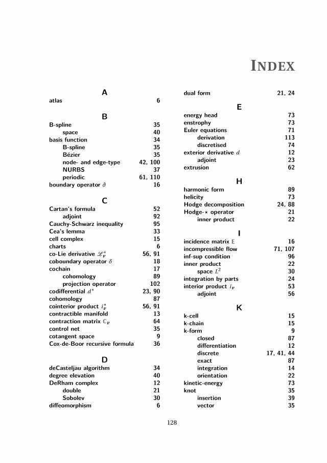
INDEX
Aatlas 6
BB-spline 35
space 40basis function 34
B-spline 35Bézier 35node- and edge-type 42, 100NURBS 37periodic 61, 110
boundary operator ∂ 16
CCartan’s formula 52
adjoint 92Cauchy-Schwarz inequality 95Cea’s lemma 33cell complex 15charts 6co-Lie derivative L ∗
v 56, 91coboundary operator δ 18cochain 17
cohomology 89projection operator 102
codifferential d∗ 23, 90cohomology 87cointerior product i∗v 56, 91contractible manifold 13contraction matrix Cv 64control net 35cotangent space 9Cox-de-Boor recursive formula 36
DdeCasteljau algorithm 34degree elevation 40DeRham complex 12
double 21Sobolev 30
diffeomorphism 6
dual form 21, 24
Eenergy head 73enstrophy 73Euler equations 71
derivation 113discretised 74
exterior derivative d 12adjoint 23
extrusion 62
Hharmonic form 89helicity 73Hodge decomposition 24, 88Hodge-? operator 21
inner product 22
Iincidence matrix E 16incompressible flow 71, 107inf-sup condition 96inner product 22
space L2 30integration by parts 24interior product iv 53
adjoint 56
Kk-cell 15k-chain 15k-form 9
closed 87differentiation 12discrete 17, 41, 44exact 87integration 14orientation 22
kinetic-energy 73knot 35
insertion 39vector 35
128

INDEX 129
LLaplace operator ∆ 24Lax-Milgram 96Lie-derivative Lv 52
adjoint 56space-time 61
Mmanifold M 6mass matrix M 45metric 55
Nnilpotency 12, 53
Oorientation 8, 11
PPoincaré inequality 95Poincaré lemma 13, 87Poisson problem 31
discretised 45well-posedness 95
potential flow 24potential function 13
pull-back operator φ∗ 93
Sscalar advection 57
discretised 65Sobolev space Wd 30Stokes’ flow 25Stokes’ theorem 14stream function 25, 107
Ttangent space 8Taylor vortices 77time integrator 75Tonti diagram 25transport theorem 57, 105
Vvector 7
field 52isomorphisms 54
Wwedge product ∧ 10
discrete 63


![Stevie Ray Vaughan : The Sky Is Crying [Songbook]](https://img.pdfslide.net/doc/110x75/5479ddc8b4af9fa42c8b46c7/stevie-ray-vaughan-the-sky-is-crying-songbook.jpg)


![Stevie Ray Vaughan - Mary Had a Little Lamb [Guitar Techniques]](https://img.pdfslide.net/doc/110x75/553cc1395503467d318b4b28/stevie-ray-vaughan-mary-had-a-little-lamb-guitar-techniques.jpg)