ORIGINAL RESEARCH FOR INQUISITIVE INVESTORS

BRANDES.COM/INSTITUTE BRANDESINSTITUTE@BRANDES.COM

MARKET TIMING: Opportunities and Risks by Wim Antoons

PAGE 2

IntroductionAsset allocation decisions, particularly those involving market timing, create both opportunities and pitfalls for investors. In the aftermath of the crash of October 1987, many investors sought protection of capital through market timing or tactical asset allocation strategies. Since then, the popularity of tactical asset allocation has increased both for professional investment managers and individual investors alike.

In this paper, I explore opportunities for enhancing returns using tactical asset allocation and market timing, as well as the challenges posed by market timing, including higher costs and the risk of missing the best-performing days of the market. I examine whether investors can succeed using tactical asset allocation and market timing strategies and look to behavioral finance concepts to explain why investors continue to embrace market timing in their investment process.

I find that strategic asset allocation was the most important driver of long-term investment success. This is because most market timers typically fail to accurately predict important equity market swings. The long-term odds are not in favor of market timing strategies.

The long-term odds are not in favor of market timing strategies.

Strategic asset allocation involves setting target allocations for various asset classes—based on factors such as time horizon, long-term investment objectives and risk tolerance—and periodically rebalancing a portfolio when it deviates from the allocation settings. Strategic asset allocation is compatible with a

“buy-and-hold” strategy.

Tactical asset allocation is an active portfolio strategy that seeks to take advantage of market pricing in the short term.

Market timing is the process of attempting to predict the future direction of the market and switching between asset classes and cash with the goal of profiting from changes in market outlook.

Executive Summary• Strategic asset allocation has been the most important driver of long-term investing

success; the long-term odds are not in favor of market timing strategies.• For market timers with a long-term horizon, it was more important to forecast bull

markets correctly than to get bear markets correct.• It is often noted that a very small proportion of high volatility days can account for the

equivalent of substantially all of long-term returns. But a strategy of trying to invest on the “best days” and avoid the “worst days” would be virtually impossible to execute.

• Any market timing strategy is likely to increase both trading and opportunity costs.• The advice of market timing newsletters was generally wrong more than right.• Mutual fund investors on average historically have tended to underperform the returns

of the funds in which they invest, largely due to poor timing of buy/sell decisions.• Investors face behavioral challenges in market timing as they tend to be poor forecasters,

yet are overconfident in the accuracy of their forecasts. • In general, market timing is detrimental to a sound and disciplined investment process; any

tactical asset allocation (market timing) should be strictly disciplined and limited in scope.

PAGE 3

I. Opportunity for Enhancing Returns

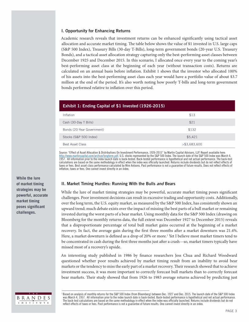
Academic research reveals that investment returns can be enhanced significantly using tactical asset allocation and accurate market timing. The table below shows the value of $1 invested in U.S. large caps (S&P 500 Index), Treasury Bills (30-day T-Bills), long-term government bonds (20-year U.S. Treasury Bonds), and a tactical asset allocation strategy capturing only the best-performing asset classes between December 1925 and December 2015. In this scenario, I allocated once every year to the coming year’s best-performing asset class at the beginning of each year (without transaction costs). Returns are calculated on an annual basis before inflation. Exhibit 1 shows that the investor who allocated 100% of his assets into the best-performing asset class each year would have a portfolio value of about $3.7 million at the end of the period. It’s also worth noting how poorly T-bills and long-term government bonds performed relative to inflation over this period.

1 Based on analysis of monthly returns for the S&P 500 Index (from Bloomberg) between Dec. 1927 and Dec. 2015. The launch date of the S&P 500 Index was March 4, 1957. All information prior to the index launch date is back-tested. Back-tested performance is hypothetical and not actual performance. The back-test calculations are based on the same methodology in effect when the index was officially launched. Returns include dividends but do not reflect effects of taxes or fees. Past performance is not a guarantee of future results. One cannot invest directly in an index.

Exhibit 1: Ending Capital of $1 Invested (1926-2015)

Inflation $13

Cash (30-Day T Bills) $21

Bonds (20-Year Government) $132

Stocks (S&P 500 Index) $5,421

Best Asset Class >$3,683,600

Source: “Effect of Asset Allocation & Distributions On Investment Performance, 1926-2015” by Martin Capital Advisors, LLP. Report available here: http://www.martincapital.com/archive/longterm.pdf. U.S. stocks represented by the S&P 500 Index. The launch date of the S&P 500 Index was March 4, 1957. All information prior to the index launch date is back-tested. Back-tested performance is hypothetical and not actual performance. The back-test calculations are based on the same methodology in effect when the index was officially launched. Returns include dividends but do not reflect effects of taxes or fees. Best asset class performance calculated by Wim Antoons. Past performance is not a guarantee of future results. Does not reflect effects of inflation, taxes or fees. One cannot invest directly in an index.

II. Market Timing Hurdles: Running With the Bulls and Bears

While the lure of market timing strategies may be powerful, accurate market timing poses significant challenges. Poor investment decisions can result in excessive trading and opportunity costs. Additionally, over the long term, the U.S. equity market, as measured by the S&P 500 Index, has consistently shown an upward trend; much debate exists over the impact of missing the best parts of a bull market or remaining invested during the worst parts of a bear market. Using monthly data for the S&P 500 Index (drawing on Bloomberg for the monthly returns data, the full extent was December 1927 to December 2015) reveals that a disproportionate percentage of total bull market gains occurred at the beginning of a market recovery. In fact, the average gain during the first three months after a market downturn was 21.4%. Here, a market downturn is defined as a drop of 20% or more.1 Yet I believe most market timers tend to be concentrated in cash during the first three months just after a crash—so, market timers typically have missed most of a recovery’s upside.

An interesting study published in 1986 by finance researchers Jess Chua and Richard Woodward questioned whether poor results achieved by market timing result from an inability to avoid bear markets or the tendency to miss the early part of a market recovery. Their research showed that to achieve investment success, it was more important to correctly forecast bull markets than to correctly forecast bear markets. Their study showed that from 1926 to 1983 average returns achieved by predicting just

While the lure of market timing strategies may be powerful, accurate market timing poses significant challenges.

PAGE 4

50% of bull markets underperformed buy-and-hold strategies, even when bear markets were forecasted with perfect accuracy.2 They concluded that for market timing to pay off, investors required accurate forecasts in at least:

• 80% of the bull and 50% of the bear markets; or• 70% of the bull and 80% of the bear markets; or • 60% of the bull and 90% of the bear markets.

Average returns achieved by predicting just 50% of bull markets underperformed buy-and-hold strategies, even when bear markets were forecasted with perfect accuracy.

III. The 25 Best and Worst Trading Days in the Stock Market

Believers in market timing argue that returns can be increased dramatically by avoiding the worst days in the stock market. On the flip side, non-believers argue that missing the best days in the stock market decimates long-term returns. I tested both hypotheses by examining monthly returns for the S&P 500 Index from January 1961 to the end of December 2015.

As shown in the table below, the results are compelling. The buy-and-hold investor would have realized an annual return of 9.87%. The perfectly accurate market timer who avoided the 25 worst trading days would have generated an annual return of 15.27%, before fees and taxes. However, the investor who missed the best 25 days realized an annual return of only 5.74%.

2 Chua, Jess H. and Richard S. Woodward. “Gains from Stock Market Timing.” Monograph Series in Finance and Economics. Monograph 1986-2. Salomon Brothers Center for the Study of Financial Institutions. Graduate School of Business Administration, New York University.

Long-Term Trends Have Been Against the Market Timer

My analysis of monthly returns for the S&P 500 Index from December 1927 until December 2015 shows:

• 12 bear markets (defined as more than 20% losses in the equity market) • 13 bull markets • Average bull market gain of 179.8% • Average bear market loss of -35.75% • Average bull market lasted 66 months • Average bear market lasted 16 months • 27% of monthly returns during bear markets were positive

U.S. stocks represented by the S&P 500 Index. The launch date of the S&P 500 Index was March 4, 1957. All information prior to the index launch date is back-tested. Back-tested performance is hypothetical and not actual performance. The back-test calculations are based on the same methodology in effect when the index was officially launched. Returns include dividends but do not reflect effects of taxes or fees. Past performance is not a guarantee of future results. Please note that all indices are unmanaged and are not available for direct investment.

Exhibit 2: Avoiding the Worst Days Would Have Outperformed Buy and HoldThe Results of Market Timing for the S&P 500 Index (1/1/1961 to 12/31/2015)

Annualized Return (%) Growth of $100

Missing 25 Best Days 5.74 $831

Missing 25 Worst Days 15.27 $21,886

Buy and Hold 9.87 $3,550

Missing Worst & Best Days 10.94 $5,125

Source: S&P 500 Index via Bloomberg, as of 12/31/15. Past performance is not a guarantee of future results. One cannot invest directly in an index. Does not reflect the effects of fees and taxes.

The results show that long-term returns were actually realized in very short periods of time. Extending the analysis, returns for the best 81 trading days during the period (out of 13,844 trading days) would have equaled the total return for a buy-and-hold investor over the entire period. In other words, with perfect foresight, being invested only 0.59% of the time would produce the same results as if an investment were held over the entire 55-year period. Or, from a different perspective, had one missed these 81 best-performing days, the annualized return during the period would fall to a meager 0.03%.

The results show that long-term returns were actually realized in very short periods of time.

PAGE 5

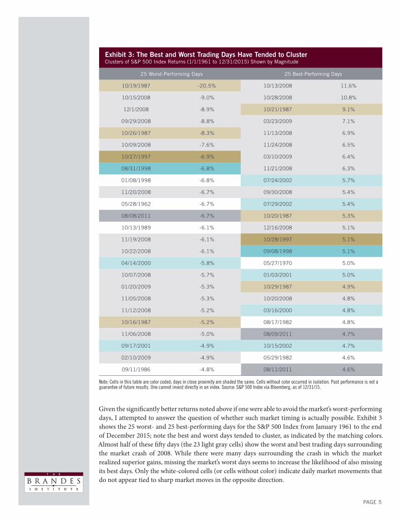
Exhibit 3: The Best and Worst Trading Days Have Tended to ClusterClusters of S&P 500 Index Returns (1/1/1961 to 12/31/2015) Shown by Magnitude

25 Worst-Performing Days 25 Best-Performing Days

10/19/1987 -20.5% 10/13/2008 11.6%

10/15/2008 -9.0% 10/28/2008 10.8%

12/1/2008 -8.9% 10/21/1987 9.1%

09/29/2008 -8.8% 03/23/2009 7.1%

10/26/1987 -8.3% 11/13/2008 6.9%

10/09/2008 -7.6% 11/24/2008 6.5%

10/27/1997 -6.9% 03/10/2009 6.4%

08/31/1998 -6.8% 11/21/2008 6.3%

01/08/1998 -6.8% 07/24/2002 5.7%

11/20/2008 -6.7% 09/30/2008 5.4%

05/28/1962 -6.7% 07/29/2002 5.4%

08/08/2011 -6.7% 10/20/1987 5.3%

10/13/1989 -6.1% 12/16/2008 5.1%

11/19/2008 -6.1% 10/28/1997 5.1%

10/22/2008 -6.1% 09/08/1998 5.1%

04/14/2000 -5.8% 05/27/1970 5.0%

10/07/2008 -5.7% 01/03/2001 5.0%

01/20/2009 -5.3% 10/29/1987 4.9%

11/05/2008 -5.3% 10/20/2008 4.8%

11/12/2008 -5.2% 03/16/2000 4.8%

10/16/1987 -5.2% 08/17/1982 4.8%

11/06/2008 -5.0% 08/09/2011 4.7%

09/17/2001 -4.9% 10/15/2002 4.7%

02/10/2009 -4.9% 05/29/1982 4.6%

09/11/1986 -4.8% 08/11/2011 4.6%

Note: Cells in this table are color coded; days in close proximity are shaded the same. Cells without color occurred in isolation. Past performance is not a guarantee of future results. One cannot invest directly in an index. Source: S&P 500 Index via Bloomberg, as of 12/31/15.

Given the significantly better returns noted above if one were able to avoid the market’s worst-performing days, I attempted to answer the question of whether such market timing is actually possible. Exhibit 3 shows the 25 worst- and 25 best-performing days for the S&P 500 Index from January 1961 to the end of December 2015; note the best and worst days tended to cluster, as indicated by the matching colors. Almost half of these fifty days (the 23 light gray cells) show the worst and best trading days surrounding the market crash of 2008. While there were many days surrounding the crash in which the market realized superior gains, missing the market’s worst days seems to increase the likelihood of also missing its best days. Only the white-colored cells (or cells without color) indicate daily market movements that do not appear tied to sharp market moves in the opposite direction.

PAGE 6

Looking back at Exhibit 2, an investor who missed both the 25 best- and worst-trading days would have realized an annual return of 10.94%, greater than the buy-and-hold investor. However, in my opinion, an investment strategy that attempts to miss both the best and the worst days is flawed. I disagree with researchers such as Mebane Faber who wrote in “Where the Black Swans Hide and The 10 Best Days Myth”3 that: “We continue to advocate that investors attempt to avoid declining markets where most of the volatility lies and conclude that market timing and risk management is indeed possible, and beneficial to the investor.” My concern with this line of thinking stems from my observation that the best trading days, as shown in Exhibit 3, often follow the worst trading days. I believe many investors panic when they see a bad trading day and sell, thus locking in their losses and eliminating the potential to participate in subsequent rebounds. Further, I do not believe that it is possible to consistently predict market performance—especially during these days when volatile returns (both up and down) have tended to cluster.

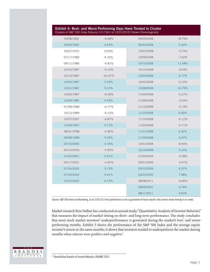
Exhibit 4 shows the same best- and worst-performing days featured in Exhibit 3, but arranged chronologically. There are a number of periods in which the stock market started with a sell-off followed by a recovery. Investors who sold after that first market correction likely missed the subsequent best-performing days and ended up with very poor long-term returns. The colored cells (blue for positive and gray for negative) reflect days when I considered positive and negative returns to “cluster.”

3 “Where The Black Swans Hide & the 10 Best Days Myth.” Faber, Mebane, Cambria Investment Management. Quantitative Research Monthly, 2011. http://papers.ssrn.com/sol3/papers.cfm?abstract_id=1908469

In my opinion, an investment strategy that attempts to miss both the best and the worst days is flawed.

PAGE 7

Exhibit 4: Best- and Worst-Performing Days Have Tended to Cluster Clusters of S&P 500 Index Returns (1/1/1961 to 12/31/2015) Shown Chronologically

05/28/1962 -6.68% 09/29/2008 -8.79%

05/29/1962 4.65% 09/30/2008 5.42%

05/27/1970 5.02% 10/07/2008 -5.74%

07/17/1982 4.76% 10/09/2008 -7.62%

09/11/1986 -4.81% 10/13/2008 11.58%

10/16/1987 -5.16% 10/15/2008 -9.03%

10/19/1987 -20.47% 10/20/2008 4.77%

10/20/1987 5.33% 10/22/2008 -6.10%

10/21/1987 9.10% 10/28/2008 10.79%

10/26/1987 -8.28% 11/05/2008 -5.27%

10/29/1987 4.93% 11/06/2008 -5.03%

01/08/1988 -6.77% 11/12/2008 -5.19%

10/13/1989 -6.13% 11/13/2008 6.92%

10/27/1997 -6.87% 11/19/2008 -6.12%

10/28/1997 5.12% 11/20/2008 -6.71%

08/31/1998 -6.80% 11/21/2008 6.32%

09/08/1998 5.09% 11/24/2008 6.47%

03/16/2000 4.76% 12/01/2008 -8.93%

04/14/2000 -5.83% 12/16/2008 5.14%

01/03/2001 5.01% 01/20/2009 -5.28%

09/17/2001 -4.92% 02/01/2009 -4.91%

07/24/2002 5.73% 03/10/2009 6.37%

07/29/2002 5.41% 03/23/2009 7.08%

10/15/2002 4.73% 08/08/2011 -6.66%

08/09/2001 4.74%

08/11/2011 4.63%

Source: S&P 500 Index via Bloomberg, as of 12/31/15. Past performance is not a guarantee of future results. One cannot invest directly in an index.

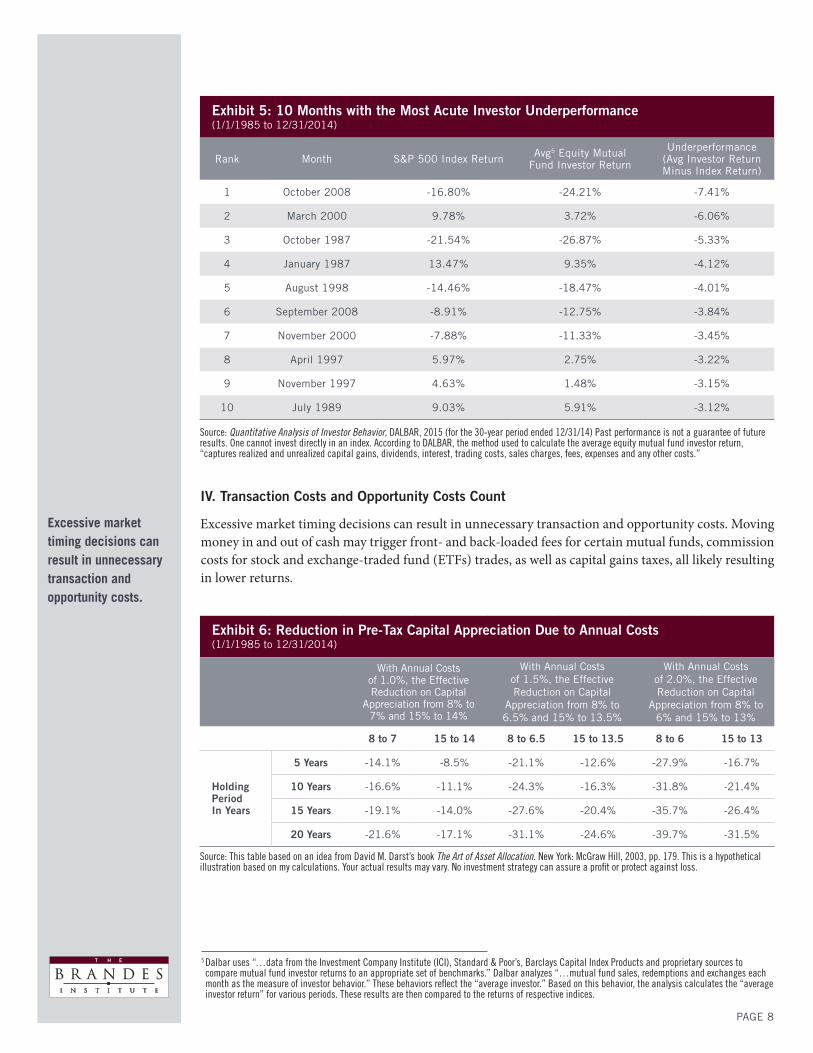
Market research firm Dalbar has conducted an annual study, “Quantitative Analysis of Investor Behavior,” that measures the impact of market timing on short- and long-term performance. The study concludes that most stock market investors’ underperformance is generated during the market’s best- and worst-performing months. Exhibit 5 shows the performance of the S&P 500 Index and the average equity investor’s return in the same months; it shows that investors tended to underperform the market during months when returns were positive and negative.4

4 “Quantitative Analysis of Investor Behavior, DALBAR, 2015.

PAGE 8

Exhibit 5: 10 Months with the Most Acute Investor Underperformance(1/1/1985 to 12/31/2014)

Rank Month S&P 500 Index Return Avg5 Equity Mutual Fund Investor Return

Underperformance(Avg Investor Return Minus Index Return)

1 October 2008 -16.80% -24.21% -7.41%

2 March 2000 9.78% 3.72% -6.06%

3 October 1987 -21.54% -26.87% -5.33%

4 January 1987 13.47% 9.35% -4.12%

5 August 1998 -14.46% -18.47% -4.01%

6 September 2008 -8.91% -12.75% -3.84%

7 November 2000 -7.88% -11.33% -3.45%

8 April 1997 5.97% 2.75% -3.22%

9 November 1997 4.63% 1.48% -3.15%

10 July 1989 9.03% 5.91% -3.12%

Source: Quantitative Analysis of Investor Behavior, DALBAR, 2015 (for the 30-year period ended 12/31/14) Past performance is not a guarantee of future results. One cannot invest directly in an index. According to DALBAR, the method used to calculate the average equity mutual fund investor return, “captures realized and unrealized capital gains, dividends, interest, trading costs, sales charges, fees, expenses and any other costs.”

5 Dalbar uses “…data from the Investment Company Institute (ICI), Standard & Poor’s, Barclays Capital Index Products and proprietary sources to compare mutual fund investor returns to an appropriate set of benchmarks.” Dalbar analyzes “…mutual fund sales, redemptions and exchanges each month as the measure of investor behavior.” These behaviors reflect the “average investor.” Based on this behavior, the analysis calculates the “average investor return” for various periods. These results are then compared to the returns of respective indices.

Excessive market timing decisions can result in unnecessary transaction and opportunity costs.

Exhibit 6: Reduction in Pre-Tax Capital Appreciation Due to Annual Costs (1/1/1985 to 12/31/2014)

With Annual Costs of 1.0%, the Effective Reduction on Capital

Appreciation from 8% to 7% and 15% to 14%

With Annual Costs of 1.5%, the Effective Reduction on Capital

Appreciation from 8% to 6.5% and 15% to 13.5%

With Annual Costs of 2.0%, the Effective Reduction on Capital

Appreciation from 8% to 6% and 15% to 13%

8 to 7 15 to 14 8 to 6.5 15 to 13.5 8 to 6 15 to 13

Holding PeriodIn Years

5 Years -14.1% -8.5% -21.1% -12.6% -27.9% -16.7%

10 Years -16.6% -11.1% -24.3% -16.3% -31.8% -21.4%

15 Years -19.1% -14.0% -27.6% -20.4% -35.7% -26.4%

20 Years -21.6% -17.1% -31.1% -24.6% -39.7% -31.5%

Source: This table based on an idea from David M. Darst’s book The Art of Asset Allocation. New York: McGraw Hill, 2003, pp. 179. This is a hypothetical illustration based on my calculations. Your actual results may vary. No investment strategy can assure a profit or protect against loss.

IV. Transaction Costs and Opportunity Costs Count

Excessive market timing decisions can result in unnecessary transaction and opportunity costs. Moving money in and out of cash may trigger front- and back-loaded fees for certain mutual funds, commission costs for stock and exchange-traded fund (ETFs) trades, as well as capital gains taxes, all likely resulting in lower returns.

PAGE 9

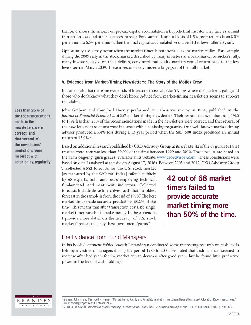
Less than 25% of the recommendations made in the newsletters were correct, and that several of the newsletters’ predictions were incorrect with astonishing regularity.

6 Graham, John R. and Campbell R. Harvey. “Market Timing Ability and Volatility Implied in Investment Newsletters’ Asset Allocation Recommendations.” NBER Working Paper #4890. October 1994.7 Damodaran, Aswath. Investment Fables: Exposing the Myths of the “Can’t Miss” Investment Strategies. New York: Prentice Hall, 2004. pp. 499-500.

42 out of 68 market timers failed to provide accurate market timing more than 50% of the time.

Exhibit 6 shows the impact on pre-tax capital accumulation a hypothetical investor may face as annual transaction costs and other expenses increase. For example, if annual costs of 1.5% lower returns from 8.0% per annum to 6.5% per annum, then the final capital accumulated would be 31.1% lower after 20 years.

Opportunity costs may occur when the market timer is not invested as the market rallies. For example, during the 2009 rally in the stock market, described by many investors as a bear-market or sucker’s rally, many investors stayed on the sidelines, convinced that equity markets would return back to the low levels seen in March 2009. These investors likely missed a large part of the bull market.

V. Evidence from Market-Timing Newsletters: The Story of the Motley Crew

It is often said that there are two kinds of investors: those who don’t know where the market is going and those who don’t know what they don’t know. Advice from market-timing newsletters seems to support this claim.

John Graham and Campbell Harvey performed an exhaustive review in 1994, published in the Journal of Financial Economics, of 237 market-timing newsletters. Their research showed that from 1980 to 1992 less than 25% of the recommendations made in the newsletters were correct, and that several of the newsletters’ predictions were incorrect with astonishing regularity. One well-known market-timing advisor produced a 5.4% loss during a 13-year period when the S&P 500 Index produced an annual return of 15.9%.6

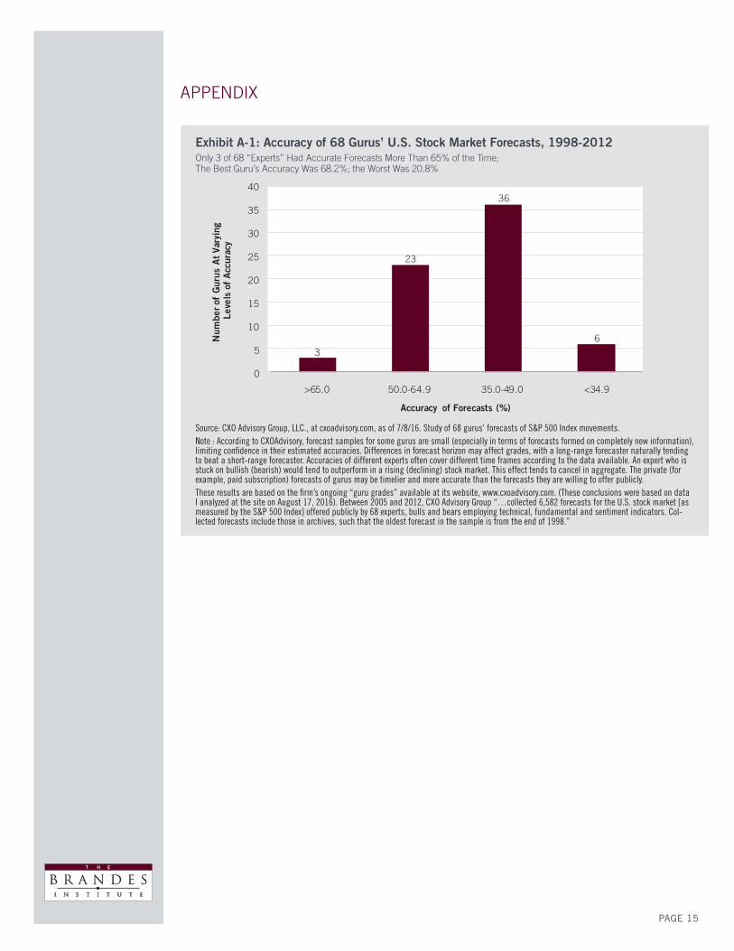
Based on additional research published by CXO Advisory Group at its website, 42 of the 68 gurus (61.8%) tracked were accurate less than 50.0% of the time between 1999 and 2012. These results are based on the firm’s ongoing “guru grades” available at its website, www.cxoadvisory.com. (These conclusions were based on data I analyzed at the site on August 17, 2016). Between 2005 and 2012, CXO Advisory Group

“…collected 6,582 forecasts for the U.S. stock market [as measured by the S&P 500 Index] offered publicly by 68 experts, bulls and bears employing technical, fundamental and sentiment indicators. Collected forecasts include those in archives, such that the oldest forecast in the sample is from the end of 1998.” The best market timer made accurate predictions 68.2% of the time. This means that after transaction costs, no single market timer was able to make money. In the Appendix, I provide more detail on the accuracy of U.S. stock market forecasts made by these investment “gurus.”

The Evidence from Fund ManagersIn his book Investment Fables Aswath Damodaran conducted some interesting research on cash levels held by investment managers during the period 1980 to 2001. He noted that cash balances seemed to increase after bad years for the market and to decrease after good years, but he found little predictive power in the level of cash holdings.7

PAGE 10

Damodaran also noted that after the crash of 1987, many mutual fund managers claimed that they could have saved investors money by steering them out of equities before the crash. They argued they could have moved between stocks, bonds and T-bills in advance of major market movements and this would have allowed investors to earn higher returns. Yet during the ‘90s, returns delivered by these funds fell short of their promises. Analyzing returns between 1994-1998 and 1989-1998, he shows that the

“S&P 500” (which reflected the performance of the overall stock market), delivered a higher average annual return (more than 15.0% annualized in the 5- and 10-year periods studied) vs. 12 so-called “Asset Allocation” funds that sought to avoid losses and deliver better-than-stock market returns (which gained about 12.0% and 10.0% annualized during the 5- and 10-year periods, respectively).

These results underscore the notion that buy-and-hold strategies historically have outperformed efforts to time the market. Another much broader study of returns for more than 400 U.S. mutual funds between 1976 and 1994 found “no evidence that funds have significant market-timing ability.8

Evidence in the Market

In a 1994 article titled “The Folly of Stock Market Timing,” R.H. Jeffrey examined the effects of moving assets between the S&P 500 Index and Treasury bills between 1975 and 1982 (using annual timing intervals) and concluded that the potential downside vastly exceeded the potential upside. (While Jeffrey focused much of his attention on this 8-year period, he also analyzed market-timing results between 1926 and 1982 and several periods within that multi-decade span. Summarizing his findings, he wrote, “The point of these charts and statistics is simply to emphasize that a market-timing strategist has tremendous natural odds to overcome, and that these odds increase geometrically with the length of the time frame and with the frequency of the timing interval.” In fact, he determined that the process of allocating assets from stocks to cash and back may result in missing out on the best years of the market.

Using a measure Jeffrey called the “compression effect,” he quantified “…the degree to which the overall positive real return from the S&P [500 Index] depended on ‘being present’ in equities during the few periods when real equity returns were high.” His compression effect was calculated at the end of the period by removing sequentially the best quarter’s returns for the S&P 500 Index in his study, then the second-best quarter and so on. In essence, the compression rate refers to the percentage of holding periods with the most influence on the results from perfectly timing the market. Missing these periods would have yielded a return below that of a buy-and-hold investor. The smaller this figure, the more difficult it was to beat a buy-and-hold strategy. Jeffrey added that the rationale for being fully invested lay not in the frequency with which stocks outperformed cash, but rather that most of the gains in his study were “…compressed into just a few periods, which (perversely but understandably) tend to follow particularly adverse times for stocks.” Summing up one of the many challenges for investors seeking to time the market, success “…depends on buying stocks when the prevailing view is that they should be sold, and vice versa,” Jeffrey wrote.9

Further evidence of the difficulty in effectively timing the market is provided in a detailed 1992 study conducted on the South African stock exchange. In this study, academics researched the results of perfectly accurate market timing (0%-100% equity) between South African T-bills and the JSE All Share Index (AS) over the period 1967–1989. Rebalancing was calculated on a monthly, quarterly and annual basis. A buy-and-hold strategy in the JSE All Share Index would have yielded 20.1% annually; T-bills would have yielded 8.9% annually. Perfectly accurate market timing on a monthly basis would have increased the returns to 48.8% annually. The less one rebalanced (quarterly or annually), the lower the results were.

Buy-and-hold strategies historically have outperformed efforts to time the market.

8 Becker, Connie, Wayne Ferson, David H. Myers and Michael J. Schill. “Conditional Market Timing with Benchmark Investors.” Journal of Financial Economics, Volume 52 (1999), pp. 119–148.9 Jeffrey, R.H. “The Folly of Stock Market Timing.” Harvard Business Review, Volume 84, Issue 4. 1984.

The process of allocating assets from stocks to cash and back may result in missing out on the best years of the market.

PAGE 11

Consistently incorrect timing (on a monthly basis) would have resulted in an annual loss of 23.6%. (The results of incorrect timing were better when rebalancing on an annual basis.) The spread between perfect correct timing and incorrect timing was a spectacular 72.4%. The loss/gain ratio was always greater than 1.0, indicating an investor could have lost much more than he could have gained with market timing. In order to be a perfectly accurate market timer, investors needed to reverse their investment course on 42% of the observations. The compression rate in this study was always about +/-10%. In other words, in order to gain with perfect market timing, you would have needed to be accurate in at least 87.4% of the switches. If you were right in 68.3% of the cases, your return would have equaled a passive buy-and-hold strategy.10 Exhibits illustrating additional results from this study are provided in the Appendix.

Evidence from Mutual Fund Investors

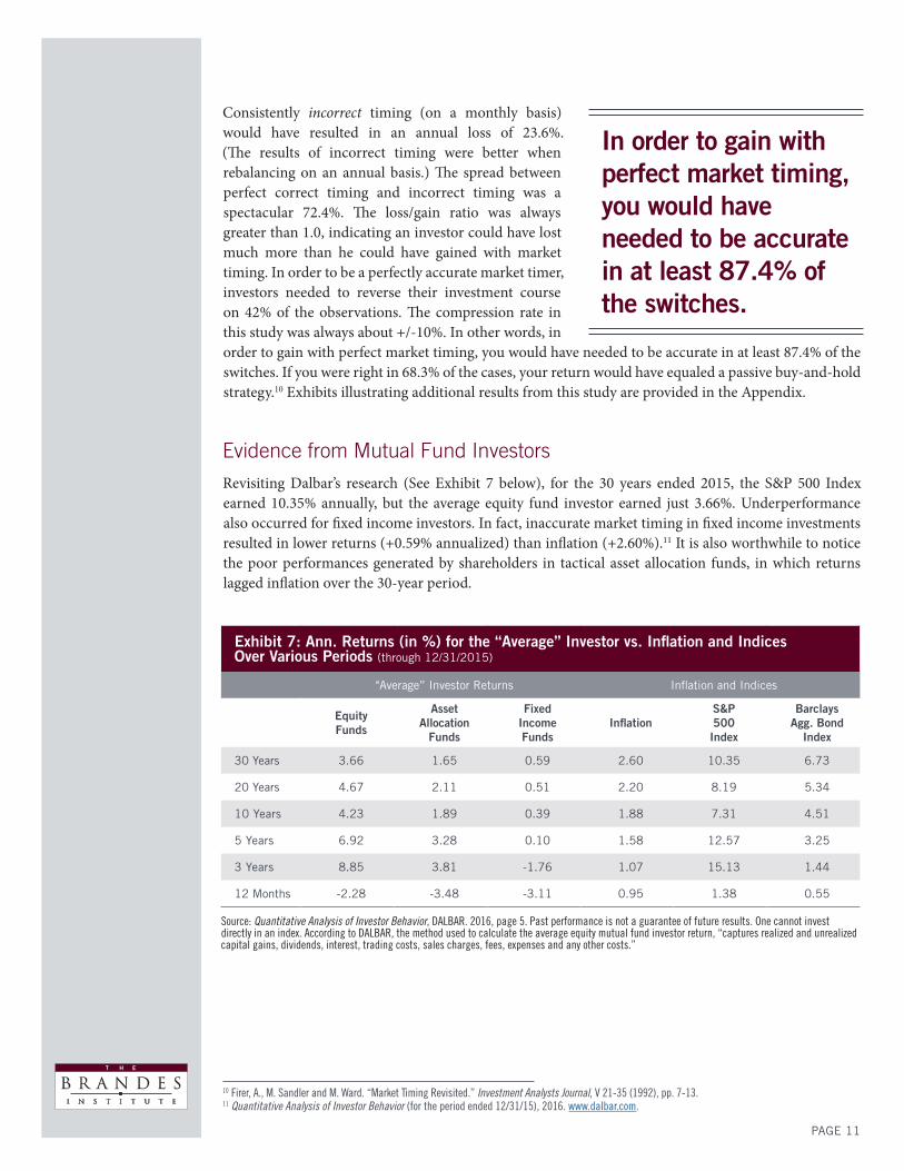
Revisiting Dalbar’s research (See Exhibit 7 below), for the 30 years ended 2015, the S&P 500 Index earned 10.35% annually, but the average equity fund investor earned just 3.66%. Underperformance also occurred for fixed income investors. In fact, inaccurate market timing in fixed income investments resulted in lower returns (+0.59% annualized) than inflation (+2.60%).11 It is also worthwhile to notice the poor performances generated by shareholders in tactical asset allocation funds, in which returns lagged inflation over the 30-year period.

In order to gain with perfect market timing, you would have needed to be accurate in at least 87.4% of the switches.

10 Firer, A., M. Sandler and M. Ward. “Market Timing Revisited.” Investment Analysts Journal, V 21-35 (1992), pp. 7-13.11 Quantitative Analysis of Investor Behavior (for the period ended 12/31/15), 2016. www.dalbar.com.

Exhibit 7: Ann. Returns (in %) for the “Average” Investor vs. Inflation and Indices Over Various Periods (through 12/31/2015)

"Average” Investor Returns Inflation and Indices

Equity Funds

Asset Allocation

Funds

Fixed Income Funds

InflationS&P 500 Index

Barclays Agg. Bond

Index

30 Years 3.66 1.65 0.59 2.60 10.35 6.73

20 Years 4.67 2.11 0.51 2.20 8.19 5.34

10 Years 4.23 1.89 0.39 1.88 7.31 4.51

5 Years 6.92 3.28 0.10 1.58 12.57 3.25

3 Years 8.85 3.81 -1.76 1.07 15.13 1.44

12 Months -2.28 -3.48 -3.11 0.95 1.38 0.55

Source: Quantitative Analysis of Investor Behavior, DALBAR. 2016, page 5. Past performance is not a guarantee of future results. One cannot invest directly in an index. According to DALBAR, the method used to calculate the average equity mutual fund investor return, “captures realized and unrealized capital gains, dividends, interest, trading costs, sales charges, fees, expenses and any other costs.”

PAGE 12

Evidence from Technical Indicators

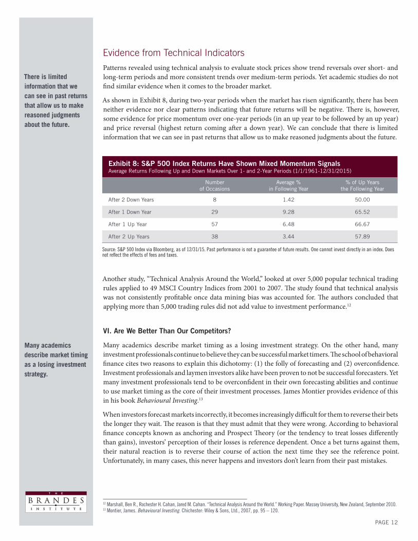
Patterns revealed using technical analysis to evaluate stock prices show trend reversals over short- and long-term periods and more consistent trends over medium-term periods. Yet academic studies do not find similar evidence when it comes to the broader market.

As shown in Exhibit 8, during two-year periods when the market has risen significantly, there has been neither evidence nor clear patterns indicating that future returns will be negative. There is, however, some evidence for price momentum over one-year periods (in an up year to be followed by an up year) and price reversal (highest return coming after a down year). We can conclude that there is limited information that we can see in past returns that allow us to make reasoned judgments about the future.

There is limited information that we can see in past returns that allow us to make reasoned judgments about the future.

Exhibit 8: S&P 500 Index Returns Have Shown Mixed Momentum Signals Average Returns Following Up and Down Markets Over 1- and 2-Year Periods (1/1/1961-12/31/2015)

Number of Occasions

Average % in Following Year

% of Up Years the Following Year

After 2 Down Years 8 1.42 50.00

After 1 Down Year 29 9.28 65.52

After 1 Up Year 57 6.48 66.67

After 2 Up Years 38 3.44 57.89

Source: S&P 500 Index via Bloomberg, as of 12/31/15. Past performance is not a guarantee of future results. One cannot invest directly in an index. Does not reflect the effects of fees and taxes.

Another study, “Technical Analysis Around the World,” looked at over 5,000 popular technical trading rules applied to 49 MSCI Country Indices from 2001 to 2007. The study found that technical analysis was not consistently profitable once data mining bias was accounted for. The authors concluded that applying more than 5,000 trading rules did not add value to investment performance.12

VI. Are We Better Than Our Competitors?

Many academics describe market timing as a losing investment strategy. On the other hand, many investment professionals continue to believe they can be successful market timers. The school of behavioral finance cites two reasons to explain this dichotomy: (1) the folly of forecasting and (2) overconfidence. Investment professionals and laymen investors alike have been proven to not be successful forecasters. Yet many investment professionals tend to be overconfident in their own forecasting abilities and continue to use market timing as the core of their investment processes. James Montier provides evidence of this in his book Behavioural Investing.13

When investors forecast markets incorrectly, it becomes increasingly difficult for them to reverse their bets the longer they wait. The reason is that they must admit that they were wrong. According to behavioral finance concepts known as anchoring and Prospect Theory (or the tendency to treat losses differently than gains), investors’ perception of their losses is reference dependent. Once a bet turns against them, their natural reaction is to reverse their course of action the next time they see the reference point. Unfortunately, in many cases, this never happens and investors don’t learn from their past mistakes.

12 Marshall, Ben R., Rochester H. Cahan, Jared M. Cahan. “Technical Analysis Around the World.” Working Paper. Massey University, New Zealand, September 2010.13 Montier, James. Behavioural Investing. Chichester: Wiley & Sons, Ltd., 2007, pp. 95 – 120.

Many academics describe market timing as a losing investment strategy.

PAGE 13

Conclusion

My belief is in line with those who believe market timing is detrimental to a sound and disciplined investment process. For example, economist J.M. Keynes believed that deviating from strategic asset allocation decisions was impractical and counterintuitive to achieving positive long-term results. In fact, deliberate short-term deviations from policy targets, he wrote, introduce substantial risks to the investment process:

“The idea of wholesale shifts is for various reasons impractical and indeed undesirable. Most of those who attempt to, sell too late and buy too late, and do both too often, incurring heavy expenses and developing too unsettled and speculative a state of mind.”14

David Swensen, manager of the Yale Endowment Fund and considered the Warren Buffett of tactical asset allocation, wrote, “Market timing explicitly moves the portfolio away from long-term policy targets, exposing the institution to avoidable risks. Because policy asset allocation provides the central means through which investors express return and risk preferences, serious investors attempt to minimize deviations from policy targets. To ensure that actual portfolios reflect desired risk and return characteristics, avoid market timing and employ rebalancing activity to keep asset classes at targeted levels.”15

My research reveals that investors tend to be overconfident in their attempts to time the market and that market timing strategies actually underperform in the long run due to transaction costs, opportunity costs and poor investment decisions. The results of the Firer, Sandler and Ward study cited earlier revealed how difficult market timing has been: a perfect market timer needed to reverse his investment course about 40% of the time. However, the compression rate was always around 10%, indicating that the ideal periods to switch were concentrated. The accuracy rate reveals a market timer needed to be right in about 70% to 80% of investment decisions; otherwise, he lost money due to transaction costs. One must also consider the gain/loss ratio, which was 1.5 or higher, meaning one could have lost more than one gained when attempting to time the market.

While many successful investors attribute their successes to superior stock picking or adherence to a sound investment discipline, I know of no single Wall Street guru who made his or her fortune using market timing. Elaine Garzarelli became a superstar on Wall Street by predicting the Wall Street crash of 1987 a few weeks in advance, and was ranked for 11 years on the “first team” in Quantitative Analysis in Institutional Investor’s all-star poll. Looking back, that was a great run. But by 1998, BusinessWeek asked,

“Remember Elaine Garzarelli? Two years ago, the investment strategist—who made her name by turning bearish a month before the 1987 crash—yelled ‘sell!’ at Dow 5400. Six months later and 1200 points higher, she turned bullish. But too late: Her bad call took Garzarelli out of the guru game.”16 Fifteen years later, in a special issue of BusinessWeek published in Spring 2003, Garzarelli predicted, "The stock market is stuck in a holding pattern for years.”17 That predication came shortly before a prolonged multi-year bull market.

It is my belief that sound investment philosophy should be based on strategic asset allocation decisions, with limited flexibility to make tactical moves. If one wishes to engage in tactical moves, they must adhere to a strict discipline. For example, a balanced portfolio may have the flexibility to deviate from 50% equity/50% fixed income to a 45% equity/55% fixed income weighting, but not be permitted to deviate further. I strongly advise against more extreme market timing decisions and always encourage decision makers to keep top of mind the trust our clients put in us to provide the best advice possible.

Andrew Duncan and William Massina contributed to this report.

14 Swensen, David. Pioneering Portfolio Management. New York: The Free Press, 2000, pp. 67.15 Swensen, David. Pioneering Portfolio Management. New York: The Free Press, 2000, pp. 73.16 Laderman, Jeffrey. “A Famous Bear Sees Honey Ahead.” BusinessWeek. Oct. 26, 1998. Issue 3601.17 Scherreik, Susan. “Elaine Garzarelli: It's All In The Timing.” BusinessWeek. Spring2003 Special Issue, Issue 3826A.

A market timer needed to be right in about 70% to 80% of investment decisions; otherwise, he lost money due to transaction costs.

PAGE 14

References

Bernstein, W., 2002. The Four Pillars of Investing, McGraw Hill, 87.

Becker, C., Ferson, W., Myers, D., Schill, M., 1998. Conditional Market Timing with Benchmark Investors, Journal of Financial Economics, Volume 52 Issue 1, 119 – 148.

BusinessWeek, March, 24th, 2003

Chua, J., Woodward, R., 1986. Gains from Stock Market Timing, Salomon Brothers Center for the Study of Financial Institutions, NY University, 12 - 13.

Dalbar, 2015. Quantitative Analysis of Investor Behavior.

Dalbar, 2016. Quantitative Analysis of Investor Behavior.

Damodaran, A., 2004. Investment Fables, Exposing the Myths of the “can’t miss” Investment Strategies, Prentice Hall, 499 – 501.

Darst, M. David, The Art of Asset Allocation, McGraw Hill, 2003, pp. 179.

Estrada, J., 2007. Black Swans and Market Timing: How not To Generate Alpha, SSRN.

Faber, M., 2011. Where the Black Swans Hide & the 10 Best Days Myth, Cambria – Quantitative Research Monthly.

Firer, A., Sandler, M., Ward, M., 1992. Market Timing Revisited, Investment Analysts Journal, Volume 21, Issue 35, 7 - 13.

Gibson, R., 2000. Asset Allocation, Mc Graw Hill, 73 – 82.

Ibbotson, R., 2015. Stocks, Bonds, Bills and Inflation 2014 Yearbook, Ibbotson Ass.

Jeffrey, H. R., 1984. The Folly of Stock Market Timing, Harvard Business Review, Volume 84, Issue 4.

Kahneman, D., Tversky, A., 2000. Choices, Values, and Frames, Cambridge University Press, Chapter 1

Marshall, R. B., Cahan, H. R., Cahan, J. 2010. Technical Analysis Around the World, SSRN.

Montier, J., 2007. Behavioural Investing, J. Wiley & Sons, Ltd., 95 – 120.

Swensen D., 2000. Pioneering Portfolio Management, The Free Press, 73.

About the Author

Wim Antoons is Head of Asset Management at Bank Nagelmackers and a member of the Brandes Institute Advisory Board. At Nagelmackers, he oversees the investment process for the private banking and fund of funds businesses. He established the firm's value investment philosophy and its open architecture fund platform. He is also co-manager of the Nagelmackers Funds and manager of the Nagelmackers Privilege Fund. Before joining Nagelmackers, he worked for 6 years in the unit-linked business at Fortis Bank Insurance, responsible for the selection of value equity funds.

PAGE 15

APPENDIX

Exhibit A-1: Accuracy of 68 Gurus’ U.S. Stock Market Forecasts, 1998-2012 Only 3 of 68 “Experts” Had Accurate Forecasts More Than 65% of the Time;The Best Guru’s Accuracy Was 68.2%; the Worst Was 20.8%

3

23

36

6

0

5

10

15

20

25

30

35

40

>65.0 50.0-64.9 35.0-49.0 <34.9

Num

ber o

f G

urus

At Va

ryin

g Le

vels

of

Acc

urac

y

Accuracy of Forecasts (%)

Source: CXO Advisory Group, LLC., at cxoadvisory.com, as of 7/8/16. Study of 68 gurus’ forecasts of S&P 500 Index movements.Note : According to CXOAdvisory, forecast samples for some gurus are small (especially in terms of forecasts formed on completely new information), limiting confidence in their estimated accuracies. Differences in forecast horizon may affect grades, with a long-range forecaster naturally tending to beat a short-range forecaster. Accuracies of different experts often cover different time frames according to the data available. An expert who is stuck on bullish (bearish) would tend to outperform in a rising (declining) stock market. This effect tends to cancel in aggregate. The private (for example, paid subscription) forecasts of gurus may be timelier and more accurate than the forecasts they are willing to offer publicly. These results are based on the firm’s ongoing “guru grades” available at its website, www.cxoadvisory.com. (These conclusions were based on data I analyzed at the site on August 17, 2016). Between 2005 and 2012, CXO Advisory Group “…collected 6,582 forecasts for the U.S. stock market [as measured by the S&P 500 Index] offered publicly by 68 experts, bulls and bears employing technical, fundamental and sentiment indicators. Col-lected forecasts include those in archives, such that the oldest forecast in the sample is from the end of 1998.”

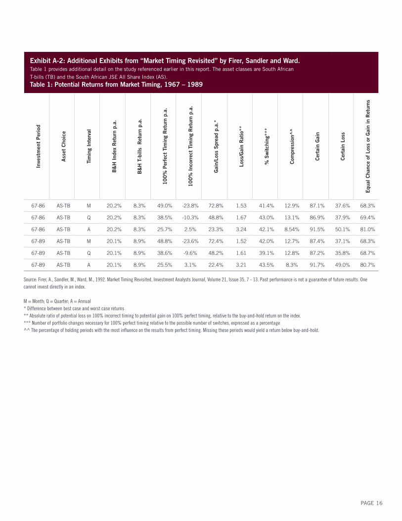
Exhibit A-2: Additional Exhibits from “Market Timing Revisited” by Firer, Sandler and Ward.Table 1 provides additional detail on the study referenced earlier in this report. The asset classes are South African

T-bills (TB) and the South African JSE All Share Index (AS).

Table 1: Potential Returns from Market Timing, 1967 – 1989

Inve

stm

ent

Per

iod

Ass

et C

hoic

e

Tim

ing

Inte

rval

B&

H I

ndex

Ret

urn

p.a.

B&

H T

-bill

s R

etur

n p.

a.

10

0%

Per

fect

Tim

ing

Ret

urn

p.a.

10

0%

Inc

orre

ct T

imin

g R

etur

n p.

a.

Gai

n/Lo

ss S

prea

d p.

a.*

Loss

/Gai

n R

atio

**

% S

wit

chin

g***

Com

pres

sion

^^

Cer

tain

Gai

n

Cer

tain

Los

s

Equ

al C

hanc

e of

Los

s or

Gai

n in

Ret

urns

67-86 AS-TB M 20.2% 8.3% 49.0% -23.8% 72.8% 1.53 41.4% 12.9% 87.1% 37.6% 68.3%

67-86 AS-TB Q 20.2% 8.3% 38.5% -10.3% 48.8% 1.67 43.0% 13.1% 86.9% 37.9% 69.4%

67-86 AS-TB A 20.2% 8.3% 25.7% 2.5% 23.3% 3.24 42.1% 8.54% 91.5% 50.1% 81.0%

67-89 AS-TB M 20.1% 8.9% 48.8% -23.6% 72.4% 1.52 42.0% 12.7% 87.4% 37.1% 68.3%

67-89 AS-TB Q 20.1% 8.9% 38.6% -9.6% 48.2% 1.61 39.1% 12.8% 87.2% 35.8% 68.7%

67-89 AS-TB A 20.1% 8.9% 25.5% 3.1% 22.4% 3.21 43.5% 8.3% 91.7% 49.0% 80.7%

PAGE 16

Source: Firer, A., Sandler, M., Ward, M., 1992. Market Timing Revisited, Investment Analysts Journal, Volume 21, Issue 35, 7 - 13. Past performance is not a guarantee of future results. One cannot invest directly in an index.

M = Month; Q = Quarter; A = Annual* Difference between best case and worst case returns** Absolute ratio of potential loss on 100% incorrect timing to potential gain on 100% perfect timing, relative to the buy-and-hold return on the index.*** Number of portfolio changes necessary for 100% perfect timing relative to the possible number of switches, expressed as a percentage^^ The percentage of holding periods with the most influence on the results from perfect timing. Missing these periods would yield a return below buy-and-hold.

PAGE 17

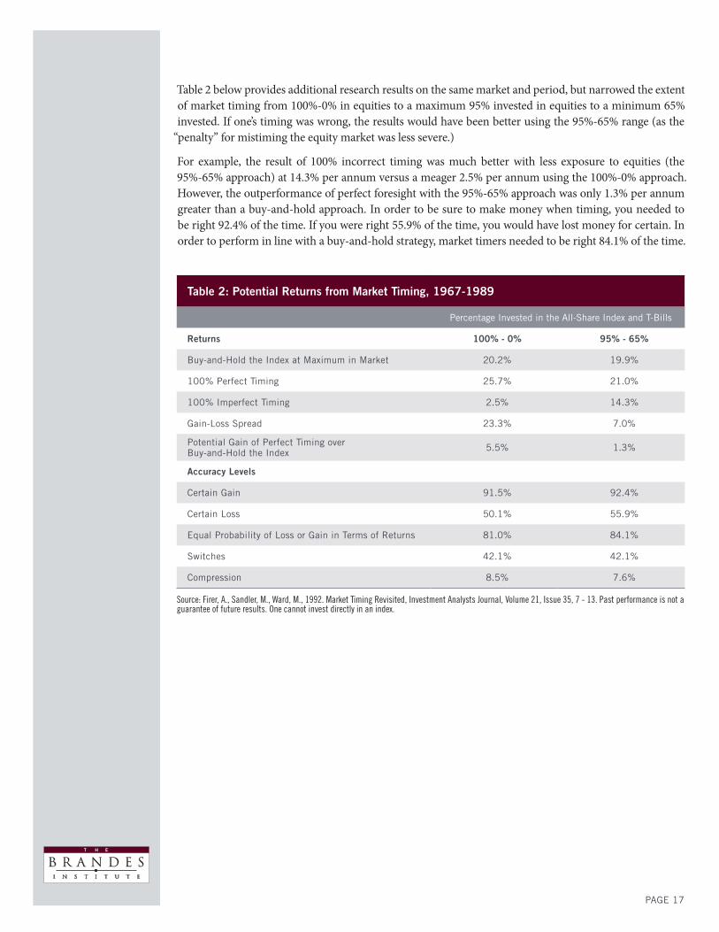
Table 2 below provides additional research results on the same market and period, but narrowed the extent of market timing from 100%-0% in equities to a maximum 95% invested in equities to a minimum 65% invested. If one’s timing was wrong, the results would have been better using the 95%-65% range (as the

“penalty” for mistiming the equity market was less severe.)

For example, the result of 100% incorrect timing was much better with less exposure to equities (the 95%-65% approach) at 14.3% per annum versus a meager 2.5% per annum using the 100%-0% approach. However, the outperformance of perfect foresight with the 95%-65% approach was only 1.3% per annum greater than a buy-and-hold approach. In order to be sure to make money when timing, you needed to be right 92.4% of the time. If you were right 55.9% of the time, you would have lost money for certain. In order to perform in line with a buy-and-hold strategy, market timers needed to be right 84.1% of the time.

Table 2: Potential Returns from Market Timing, 1967-1989

Percentage Invested in the All-Share Index and T-Bills

Returns 100% - 0% 95% - 65%

Buy-and-Hold the Index at Maximum in Market 20.2% 19.9%

100% Perfect Timing 25.7% 21.0%

100% Imperfect Timing 2.5% 14.3%

Gain-Loss Spread 23.3% 7.0%

Potential Gain of Perfect Timing over Buy-and-Hold the Index 5.5% 1.3%

Accuracy Levels

Certain Gain 91.5% 92.4%

Certain Loss 50.1% 55.9%

Equal Probability of Loss or Gain in Terms of Returns 81.0% 84.1%

Switches 42.1% 42.1%

Compression 8.5% 7.6%

Source: Firer, A., Sandler, M., Ward, M., 1992. Market Timing Revisited, Investment Analysts Journal, Volume 21, Issue 35, 7 - 13. Past performance is not a guarantee of future results. One cannot invest directly in an index.

The S&P 500 Index is a market capitalization index that measures the equity performance of 500 leading companies in industries of the U.S. economy.

The FTSE/JSE All-Share Index is designed to represent the performance of South African companies. It represents 99% of the full market capital value of South African companies, i.e. before the application of any investability weightings, of all ordinary securities listed on the main board of the Johannesburg Stock Exchange (JSE), subject to minimum freefloat and liquidity criteria.

The Bloomberg Barclays U.S. Aggregate Bond Index is a broad-based benchmark that measures the investment-grade, U.S. dollar-denominated, fixed-rate taxable bond market. This index is a total return index which reflects the price changes and interest of each bond in the index.

This material was prepared by the Brandes Institute, a division of Brandes Investment Partners®. It is intended for informational purposes only. It is not meant to be an offer, solicitation or recommendation for any products or services. The foregoing reflects the thoughts and opinions of the Brandes Institute.

The information provided in this material should not be considered a recommendation to purchase or sell any particular security. It should not be assumed that any security transactions, holdings or sectors discussed were or will be profitable, or that the investment recommendations or decisions we make in the future will be profitable or will equal the investment performance discussed herein.

Unlike bonds issued or guaranteed by the U.S. government or its agencies, stocks and other bonds are not backed by the full faith and credit of the United States. Stock and bond prices will experience market fluctuations. Please note that the value of government securities and bonds in general have an inverse relationship to interest rates. Bonds carry the risk of default, or the risk that an issuer will be unable to make income or principal payment. There is no assurance that private guarantors or insurers will meet their obligations. The credit quality of the investments in a portfolio is no guarantee of the safety or stability of the portfolio.

International and emerging markets investing is subject to certain risks such as currency fluctuation and social and political changes; such risks may result in greater share price volatility. Please note that all indices are unmanaged and are not available for direct investment.

No investment strategy can assure a profit or protect against loss.

Diversification does not assure a profit or protect against a loss in a declining market.

Brandes Investment Partners does not guarantee that the information supplied is accurate, complete or timely, or make any warranties with regard to the results obtained from its use.

Copyright © 2016 Brandes Investment Partners, L.P. ALL RIGHTS RESERVED. Brandes Investment Partners® is a registered trademark of Brandes Investment Partners, L.P. in the United States and Canada. Users agree not to copy, reproduce, distribute, publish or in any way exploit this material, except that users may make a print copy for their own personal, non-commercial use. Brief passages from any article may be quoted with appropriate credit to the Brandes Institute. Longer passages may be quoted only with prior written approval from the Brandes Institute. For more information about Brandes Institute research projects, visit our website at www.brandes.com/institute.

The Brandes Institute11988 El Camino Real Suite 600 P.O. Box 919048 San Diego CA 92191-9048858.755.0239800.237.7119

Get the Latest Research and Ideas:

BRANDES.COM/INSTITUTE BRANDESINSTITUTE@BRANDES.COM