Bypassing KLS:

Gaussian Cooling and an O∗(n3) Volume Algorithm

Ben Cousins Santosh VempalaSchool of Computer Science

Georgia Tech

April 3, 2019

Abstract

We present an O∗(n3) randomized algorithm for estimating the volume of a well-roundedconvex body given by a membership oracle, improving on the previous best complexity ofO∗(n4).The new algorithmic ingredient is an accelerated cooling schedule where the rate of coolingincreases with the temperature. Previously, the known approach for potentially achieving suchcomplexity relied on a positive resolution of the KLS hyperplane conjecture, a central openproblem in convex geometry.

1 Introduction

Computing the volume of a convex body is an ancient and fundamental problem; it is also a difficultproblem, as evidenced by both the #P-hardness of computing the volume of an explicit polytope[6] and exponential lower bounds for deterministic algorithms in the general oracle model, evento approximate the volume to within an exponential factor in the dimension [13, 14]. Againstthis backdrop, the breakthrough result of Dyer, Frieze and Kannan [8, 9] established a randomizedpolynomial-time algorithm for estimating the volume to within any desired accuracy. In the quarter-century since then, the quest for faster volume algorithms has revealed an array of powerful andelegant techniques for the design and analysis of algorithms, and influenced the development ofasymptotic convex geometry [1, 17, 7, 18, 15, 16, 3, 21, 19, 11] .

The DFK algorithm for computing the volume of a convex body K in Rn given by a membershiporacle uses a sequence of convex bodies K0,K1, . . . ,Km = K, starting with the unit ball fullycontained in K and ending with K. Each successive body Ki = 2i/nBn ∩ K is a slightly largerball intersected with K. Using random sampling, the algorithm estimates the ratios of volumes ofconsecutive bodies. The product of these ratios times the volume of the unit ball was the estimateof the volume of K. Sampling is achieved by a random walk in the convex body. There were manytechnical issues to be addressed, but the central challenge was to show a random walk that “mixed”rapidly, i.e., converged to its stationary distribution in a polynomial number of steps. The overallcomplexity of the algorithm was O∗(n23) oracle calls1.

Since then researchers have improved the complexity of volume computation and sampling forconvex bodies considerably, to O∗(n4) for volume estimation and for obtaining the first random

1The O∗ notation suppresses error terms and logarithmic factors.

1

arX

iv:1

409.

6011

v1 [

cs.D

S] 2

1 Se

p 20

14

sample [21, 19] and to O∗(n3) per sample for subsequent samples [19, 20]. These improvements relyon continuous random walks, the use of affine transformations, improved isoperimetric inequalitiesand several other developments. However, throughout the course of these developments, the outerDFK algorithm using a chain of bodies remained unchanged till most recent improvement in 2003[21]. The LV algorithm relies on sampling a sequence of logconcave distributions, akin to simulatedannealing, starting with one that is highly concentrated around a point deep inside the convex bodyand ending with the uniform distribution (we will discuss these ideas in more detail presently).The total number of random points needed is only O∗(n), down from Ω(n2) needed by all previousalgorithms. Combining this with the O∗(n3) amortized complexity for each sample yielded theoverall O∗(n4) complexity for volume computation. Before running this algorithm, there is a pre-processing step where the convex body is placed in nearly-isotropic position, ensuring in particularthat most of the body is contained in a ball of radius O(

√n). Crucially, this well-roundedness

property is maintained during the course of the algorithm.Is there a faster algorithm? In 1995, Kannan, Lovasz and Simonovits, while analyzing the

convergence of the ball walk for sampling, proposed a beautiful geometric conjecture now knownas the KLS hyperplane conjecture [15]. Roughly speaking, it says that the worst-case isoperimetricratio for a subset of a convex body is achieved by a hyperplane to within a constant factor. Theywere able to show that hyperplanes are within O(

√n) of the minimum. The convergence of the ball

walk depends on the square of the reciprocal of the isoperimetric ratio; thus the KLS conjecturehad the potential to improve the sampling time by a factor of n to O∗(n2) per sample and therebyindicated the possibility of an O∗(n3) volume algorithm (such an algorithm would have to surmountother substantial hurdles).

The KLS hyperplane conjecture remains unresolved, in spite of intensive efforts and partialprogress towards its resolution [2, 12, 11]. Indeed, it captures two well-known and much older con-jectures from convex geometry, the slicing (or hyperplane) conjecture and the thin-shell conjecture(these were all shown to be equivalent in a certain sense recently [10, 11]), and thus has effectivelyevaded resolution for nearly a half-century.

Our main finding is an O∗(n3) algorithm for any convex body containing a unit ball and mostlycontained in a ball of radius O∗(

√n). Equivalently, it suffices to have E(‖X‖2) = O∗(n) for a

uniform random point X from the body. Assuming the body is well-rounded (or sandwiched) inthis sense, no further affine transformation is used, and there is no need to assume or maintainnear-isotropy during the course of the volume algorithm.

To describe the main ideas behind the improvement, we recall the LV algorithm in more de-tail. It uses a sequence of O∗(

√n) exponential distributions, starting with a distribution that is

concentrated inside the unit ball contained in K, then “flattening” this distribution to the uniformby adjusting a multiplicative factor in the exponent2. In each phase, samples from the previousdistribution are used to estimate the ratio of the integrals of two consecutive exponential functions(by simply averaging the ratio of the function values at the sample points). It is crucial to keepthe variance of this ratio estimator bounded, and to do this, the distributions could be cooled by afactor of 1 + 1√

nin each phase. This leads to O∗(

√n) phases in total, and to O∗(

√n) samples per

phase. Along with the amortized sample complexity of O∗(n3) per sample, this gives the bound ofO∗(n4).

How could we possibly improve this without the KLS conjecture? One avenue is indicated

2In the original description, the algorithm first created a “pencil” using an extra dimension, but this can beavoided [19].

2

by our recent paper [5], which gives an O∗(n3) algorithm to compute the Gaussian measure of aconvex body, i.e., the integral of a standard Gaussian over a convex body given by a membershiporacle and containing the unit ball. This is achieved by using a sequence of Gaussians (ratherthan exponentials as in LV), starting with a highly concentrated Gaussian centered inside K andending with the standard Gaussian. The cooling schedule is the same as in the LV algorithm, buteach sample takes only O∗(n2) time. For a Gaussian distribution restricted to a convex body, thepaper gave an improved bound on the conductance. This is based on an improved isoperimetricinequality derived from the fact that the KLS conjecture holds for restrictions Gaussians to convexbodies. For a Gaussian with covariance σ2I, the mixing time was shown to be O∗(maxσ2, 1n2)(see Theorem 3.3 below). Since the start is a small σ and the last σ is 1, this bound is O∗(n2)throughout the algorithm. (There are additional technical issues such as maintaining a warm startfor the random walks, and we will encounter them here as well.)

We will also use Gaussian cooling, starting with a highly concentrated Gaussian and flatteningit (i.e., increasing σ) till we reach the uniform distribution. In the beginning, this is similar tothe algorithm of [5]. But after σ becomes higher than 1 (or some constant), we no longer havequadratic sampling time, as the mixing time of the ball work grows as maxσ2, 1n2. Moreover,we need to go till σ2 = Ω(n), so cooling at the rate of 1 + 1/

√n would be too slow. The main

new idea is that for σ > 1, the cooling rate can be made higher, in fact about 1 + σ/√n instead

of only 1 + 1/√n. This means that the number of phases to double σ2 is only

√n/σ and therefore

the number of samples per “doubling” phase is roughly also√n/σ, giving n/σ2 samples in total.

Multiplying by the sampling time, we have√nσ ·

√nσ · σ

2n2 = n3, a cubic algorithm!The key technical component of the analysis is to show that the variance of the ratio estimator

remains bounded by a constant even at this higher cooling rate. For this we use the localizationlemma of Lovasz and Simonovits. Our main result can be stated more precisely as follows. Wenote that the roundness condition can be achieved for any convex body by a preprocessing stepconsisting of an affine transformation. It is a significantly weaker condition than isotropic position.

Theorem 1.1. There is an algorithm that, for any ε > 0, p > 0 and convex body K in Rn thatcontains the unit ball and has EK(‖X‖2) = O∗(n), with probability 1− p, approximates the volumeof K within relative error ε and has complexity O∗(n3) in the membership oracle model.

More generally, if EK(‖X‖2) = R2, then the algorithm has complexity

O

(maxR2n2, n3

ε2· log4 n log2 n

εlog

1

p

)= O∗

(maxR2n2, n3

).

The current best complexity for achieving well-roundedness, i.e., R2 = O(n), for a convex bodyis O∗(n4) [21]. In previous work, the complexity of generating the first nearly uniform randompoint was always a factor significantly higher than for later points. Here, using a faster coolingschedule, we can generate the first random point in O∗(n3) steps, under the same assumption thatK is well-rounded. Any subsequent uniform random points also require O∗(n3) steps.

Theorem 1.2. There is an algorithm that, for any ε > 0, p > 0, and any convex body K in Rnthat contains the unit ball and has EK(‖X‖2) = R2, with probability 1−p, generates random pointsfrom a density ν that is within total variation distance ε from the uniform distribution on K. Inthe membership oracle model, the complexity of each random point, including the first, is

O

(maxR2n2, n3 log n log

n

εlog

n

p

)= O∗

(maxR2n2, n3

).

3

2 Algorithm

At a high level, the algorithm relies on sampling random points from a sequence of distributionsusing the ball walk with a Metropolis filter. For a target density proportional to the function f ,the ball walk with δ-steps is defined follows:

Ball walk(δ, f)

At point x:

1. Pick a random point y from x+ δBn.

2. Go to y with probability min1, f(y)/f(x).

Figure 1: The Ball walk with a Metropolis filter

After a suitable number of steps, the point x obtained will be from a distribution close to theone whose density is proportional to f . To keep the number of steps small, we need a warm start,i.e., a point whose distribution is already close to the target distribution. We describe the procedurefor obtaining a warm start after the main volume algorithm.

The algorithm starts with a Gaussian of variance 1/(4n), with mean at the center of the unit ballinside K. This variance is increased over a sequence of phases till the distribution becomes uniformover K. In the first part of the algorithm, till the variance reaches a constant, it is increased by afixed factor of 1 + 1/

√n in each phase. Thus, the number of phases required is O(

√n log n). In the

next part of the algorithm, the variance accelerates at a faster rate, by a factor of 1 + σ/(4C√n)

where σ2 is the current variance. This process is continued till the variance becomes linear in C2n,at which point one final phase can be used to jump to the uniform distribution. In each phase, wepick a sample of random points from the current distribution and compute the average of the ratioof the current density to the next density for each point. The product of these ratios times a fixedterm to account for the integral of the initial function is the estimate output by the algorithm.

Let f(σ2,K) be the function that assigns value exp(−‖x‖2/(2σ2)

)to points in a convex set K

and zero to points outside. The algorithm below uses a series of such functions.To sample efficiently from each distribution in the sequence of distributions defined in the

volume algorithm, we need to maintain a warm start, i.e., a point whose distribution is not farfrom the target distribution of that phase. To do this, we use a finer cooling schedule describedbelow, chosen so that a random point from the current distribution is a warm start for the nextdistribution.

3 Outline of analysis

The main insight that speeds up our algorithm is the cooling rate of 1 + σ/√n once σ2 > 8C2.

If we cooled at a rate of 1 + 1/√n throughout the algorithm, we would get an O∗(n4) algorithm

for computing the volume of a convex body contained in a ball of radius O∗(√n). Theorem 3.3

implies that the mixing time of the ball walk is O∗(max1, σ2n2) for a Gaussian with variance σ2.Cooling at the faster rate once σ2 > 8C2 allows us to compute volume in time O∗(n3) by havingfewer phases when the mixing time of the ball walk increases. Analogously to the analysis of the

4

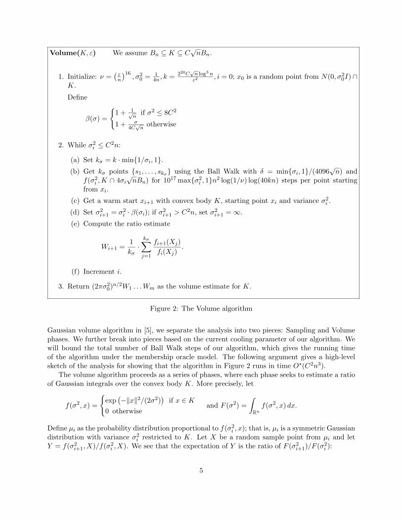
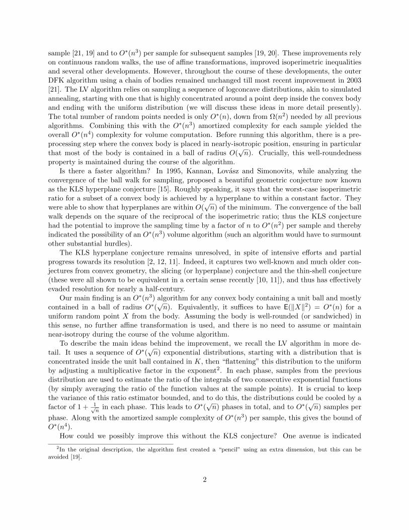
Volume(K, ε) We assume Bn ⊆ K ⊆ C√nBn.

1. Initialize: ν =(εn

)16, σ2

0 = 14n , k = 220C

√n log3 nε2

, i = 0; x0 is a random point from N(0, σ20I)∩

K.

Define

β(σ) =

1 + 1√

nif σ2 ≤ 8C2

1 + σ4C√n

otherwise

2. While σ2i ≤ C2n:

(a) Set kσ = k ·min1/σi, 1.(b) Get kσ points s1, . . . , skσ using the Ball Walk with δ = minσi, 1/(4096

√n) and

f(σ2i ,K ∩ 4σi

√nBn) for 1017 maxσ2

i , 1n2 log(1/ν) log(40kn) steps per point startingfrom xi.

(c) Get a warm start xi+1 with convex body K, starting point xi and variance σ2i .

(d) Set σ2i+1 = σ2

i · β(σi); if σ2i+1 > C2n, set σ2

i+1 =∞.

(e) Compute the ratio estimate

Wi+1 =1

kσ·kσ∑j=1

fi+1(Xj)

fi(Xj).

(f) Increment i.

3. Return (2πσ20)n/2W1 . . .Wm as the volume estimate for K.

Figure 2: The Volume algorithm

Gaussian volume algorithm in [5], we separate the analysis into two pieces: Sampling and Volumephases. We further break into pieces based on the current cooling parameter of our algorithm. Wewill bound the total number of Ball Walk steps of our algorithm, which gives the running timeof the algorithm under the membership oracle model. The following argument gives a high-levelsketch of the analysis for showing that the algorithm in Figure 2 runs in time O∗(C2n3).

The volume algorithm proceeds as a series of phases, where each phase seeks to estimate a ratioof Gaussian integrals over the convex body K. More precisely, let

f(σ2, x) =

exp

(−‖x‖2/(2σ2)

)if x ∈ K

0 otherwiseand F (σ2) =

∫Rnf(σ2, x) dx.

Define µi as the probability distribution proportional to f(σ2i , x); that is, µi is a symmetric Gaussian

distribution with variance σ2i restricted to K. Let X be a random sample point from µi and let

Y = f(σ2i+1, X)/f(σ2

i , X). We see that the expectation of Y is the ratio of F (σ2i+1)/F (σ2

i ):

5

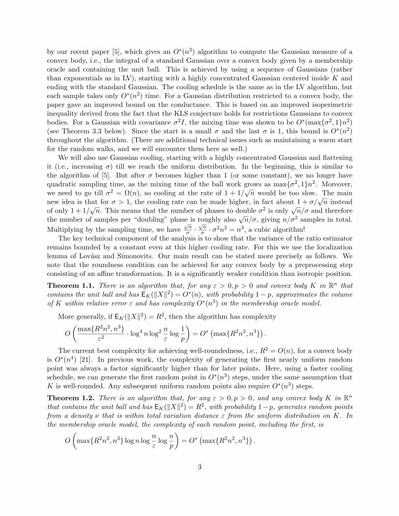
Warm start (x0, σ2start,K)

Let

α(σ) =

1 + 1

n if σ2start ≤ 8C2

1 + σ2

C2notherwise

σ2end =

σ2start(1 + 1√

n) if σ2

start ≤ 8C2

σ2start(1 + σ

4C√n

) otherwise

Set σ = σstart. While σ2 ≤ σ2end, repeat:

1. Increase σ2 by a factor of α(σ).

2. Get a point x from using the Ball walk with δ = minσ, 1/(4096√n) and f = f(σ2,K ∩

4σ√nBn) for maxσ2, 1n2 · 1017 log(1/ν) log(40kn) steps starting from x0.

Return x as the warm start.

Figure 3: Maintaining a warm start

E(Y ) =

∫K

exp

(‖x‖2

2σ2i

− ‖x‖2

2σ2i+1

)dµi(x)

=

∫K

exp

(‖x‖2

2σ2i

− ‖x‖2

2σ2i+1

)·

exp(−‖x‖2/(2σ2

i ))

F (σ2i )

dx

=1

F (σ2i )·∫K

exp

(− ‖x‖

2

2σ2i+1

)dx =

F (σ2i+1)

F (σ2i )

.

Our goal is to estimate E(Y ) within some target relative error. The volume algorithm esti-mates the quantity E(Y ) by taking random sample points X1, . . . , Xk and computing the empiricalestimate for E(Y ) from the corresponding Y1, . . . , Yk:

W =1

k

k∑j=1

Yj =1

k

k∑j=1

fi+1(Xj)

fi(Xj).

The variance of Y divided by its expectation squared will give a bound on how many independentsamples Xi are needed to estimate E(Y ) within the target accuracy. Thus we seek to boundE(Y 2)/E(Y )2. We have that

E(Y 2) =

∫K exp

(‖x‖22σ2i− ‖x‖

2

σ2i+1

)dx∫

K exp(−‖x‖

2

2σ2i

)dx

.

And therefore

E(Y 2)

E(Y )2=F (σ2

i )F (σ2i+1σ

2i

2σ2i−σ2

i+1)

F (σ2i+1)2

=F (σ2

i )F (σ2i · ( 1

2σ2i /σ

2i+1−1

))

F (σ2i+1)2

6

If we let σ2 = σ2i+1 and σ2

i = σ2/(1 + α), then we can further simplify as

E(Y 2)

E(Y )2=F(

σ2

1+α

)F(

σ2

1−α

)F (σ2)

.

The algorithm has two parts, and the cooling rate αi is different for them. In the first part,starting with a Gaussian of variance σ2 = 1/(4n), which has almost all its measure inside the ballcontained in K, we increase the variance by a fixed factor of 1+1/

√n in each phase till the variance

reaches a constant. For each σ, we sample random points from the corresponding distribution andestimate the ratio of the densities for the current phase and the next phase by averaging oversamples. The number of samples required in each phase is proportional to the number of phases,and thus both are O∗(

√n). The total complexity for the first part is thus

O∗(√n) phases×O∗(

√n) samples per phase×O∗(n2) time per sample = O∗(n3).

This is exactly the analysis carried out in [5] to sample the standard Gaussian density in a convexbody.

In the second part, we increase the variance till it reaches Ω(n), after which one final phasesuffices to compare with the target uniform distribution. However, we cannot afford to cool at thesame rate of 1 + 1/

√n because the time per sample goes to Ω(σ2n2) for σ > 1. By the end of

this part, we would be using n3 per sample, and the overall complexity would be n4. Instead weobserve that we can cool at a faster rate of 1 + σ/(4C

√n) and still maintain that the variance of

the ratio estimator is a constant.In Section 4.2, we prove the following bound.

Lemma 3.1. Let K ⊆ C√nBn, σ2 ≥ 8C2, α ≤ 1/10, and n ≥ 10. Then,

F(

σ2

1+α

)F(

σ2

1−α

)F (σ2)

≤ 1280 · exp

(7 · C

2α2n

σ2

).

Lemma 3.1 allows us to cool faster if the variance of the current Gaussian is larger; moreprecisely once σ2 ≥ 8C2, we can select

α =σ

4C√n

and the variance will be bounded by a constant.With this rate, the number of phases needed to double the variance is only O(

√n/σ), and

thus the number of samples per phase is also the same. Together, they compensate for the highercomplexity of obtaining each sample. The complexity of the second part is

O∗(√n/σ) phases×O∗(

√n/σ) samples per phase×O∗(σ2n2) time per sample = O∗(n3).

In Section 4.2, we prove that cooling at this accelerated rate still keeps the variance of the ratioestimator bounded by a constant.

To sample efficiently, we need a warm start for each phase. For two probability distributions Pand Q with state space K, the M -warmness of P and Q is defined as

M(P,Q) = supS⊆K

P (S)

Q(S).

7

To keep this parameter bounded by a constant, we use a finer-grained cooling schedule so that arandom point from one phase is a warm start for the next phase. This cooling schedule is alsodifferent in the two parts. In the first part of the algorithm, where we can cool at the rate of1 + 1/n and use O∗(n2) steps to sample. In the second part, we cool at the rate of 1 + σ2/(C2n2),and this is fast enough to compensate for the higher sample complexity of O∗(σ2n2). Thus, theoverall time to obtain a warm start for every phase of the algorithm is also O∗(n3). We analyzethis in full detail in Section 4.1, including the proof that this cooling rate maintains a warm startfrom one phase to the next.

The following lemma guarantees that the ball walk in the algorithm will always have a warmstart, i.e. the M -warmness is bounded by a constant.

Lemma 3.2. Let K ⊆ C√n · Bn, σ2

i+1 = σ2i (1 + σ2

i /(C2n)), and fi(x) = exp

(−‖x‖2/(2σ2

i )).

Denote Qi as the associated probability distributions of fi over K. Then we can bound the warmnessbetween successive phases as

M(Qi, Qi+1) ≤√e.

To prove the sampling itself is efficient, we derive the following theorem from the results of [5].

Theorem 3.3. Let K be a convex set containing the unit ball, Q0 be a starting distribution, andQ be the target Gaussian density N (0, σ2I) restricted to K ∩ 4σ

√nBn. For any ε > 0, p > 0,

the lazy Metropolis ball walk with δ-steps for δ = minσ, 1/(4096√n), starting from Q0, satisfies

dtv(Qt, Q) ≤ ε with probability 1− p after

t ≥ C ·M(Q0, Q) ·maxσ2, 1n2 log

(1

ε

)log

(1

p

)steps for an absolute constant C.

In other words, the ball walk will mix in O∗(maxσ2, 1n2) steps from a warm start.

4 Proofs

4.1 Sampling

First, we prove that the stationary distribution of each phase is a warm start for the next.Proof.(of Lemma 3.2). Note that

fi+1(x) = exp

(− ‖x‖

2

2σ2i+1

)= exp

(− ‖x‖2

2σ2i (1 + σ2

i /(C2n))

)= exp

(−‖x‖

2

2σ2i

·(

1− σ2i /(C

2n)

1 + σ2i /(C

2n)

))= fi(x) · exp

(‖x‖2

2C2n· 1

1 + σ2i /(C

2n)

)≤ fi(x) · exp

(‖x‖2

2C2n

).

8

We have that

M(Qi, Qi+1) = supS⊆K

Qi(S)

Qi+1(S)

≤∫K fi+1(x) dx∫K fi(x) dx

· supx∈K

fi(x)

fi+1(x)

=

∫K fi+1(x) dx∫K fi(x) dx

· supx∈K

(exp

(− ‖x‖

2

2C2n· 1

1 + σ2i /(C

2n)

))

=

∫K fi+1(x) dx∫K fi(x) dx

≤∫K fi(x) exp

(‖x‖2/(2C2n)

)dx∫

K fi(x) dx

≤ supx∈K

(exp

(‖x‖2

2C2n

))≤√e,

since ‖x‖ ≤ C√n.

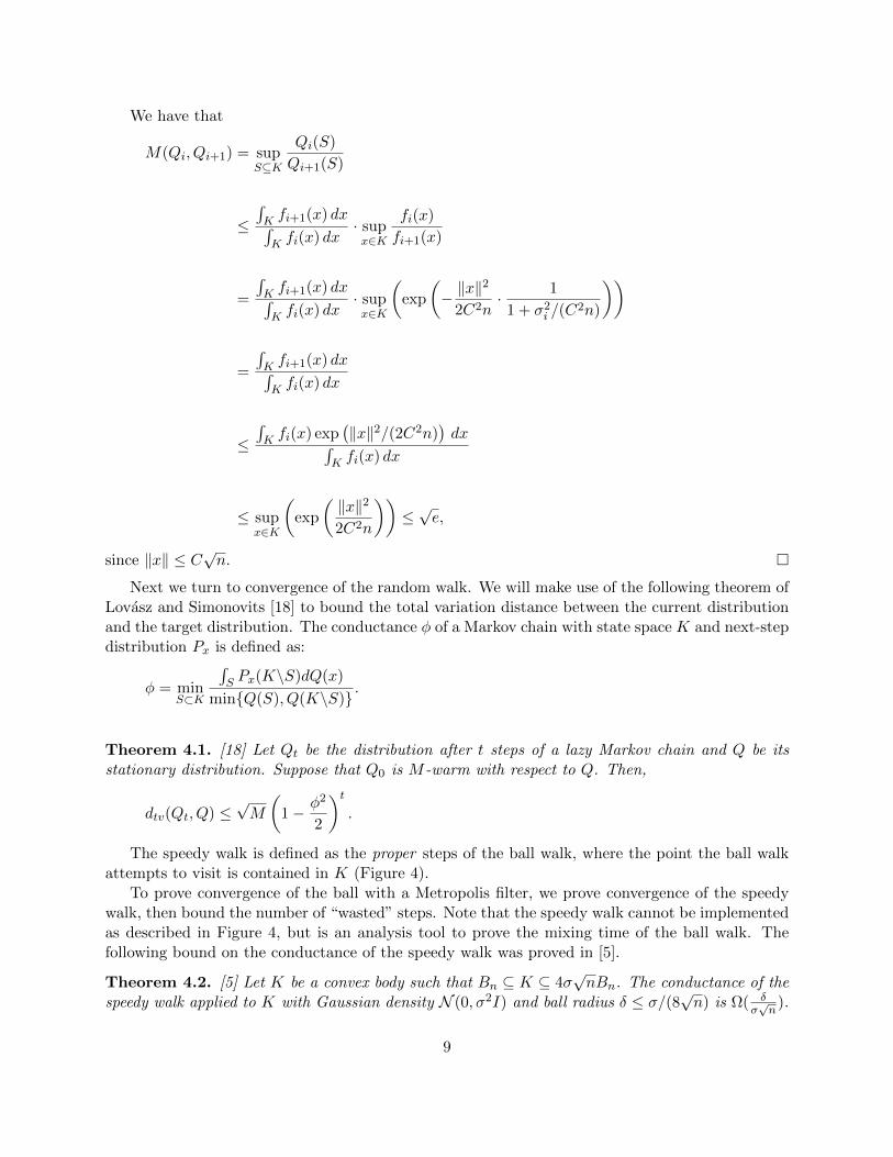
Next we turn to convergence of the random walk. We will make use of the following theorem ofLovasz and Simonovits [18] to bound the total variation distance between the current distributionand the target distribution. The conductance φ of a Markov chain with state space K and next-stepdistribution Px is defined as:

φ = minS⊂K

∫S Px(K\S)dQ(x)

minQ(S), Q(K\S).

Theorem 4.1. [18] Let Qt be the distribution after t steps of a lazy Markov chain and Q be itsstationary distribution. Suppose that Q0 is M -warm with respect to Q. Then,

dtv(Qt, Q) ≤√M

(1− φ2

2

)t.

The speedy walk is defined as the proper steps of the ball walk, where the point the ball walkattempts to visit is contained in K (Figure 4).

To prove convergence of the ball with a Metropolis filter, we prove convergence of the speedywalk, then bound the number of “wasted” steps. Note that the speedy walk cannot be implementedas described in Figure 4, but is an analysis tool to prove the mixing time of the ball walk. Thefollowing bound on the conductance of the speedy walk was proved in [5].

Theorem 4.2. [5] Let K be a convex body such that Bn ⊆ K ⊆ 4σ√nBn. The conductance of the

speedy walk applied to K with Gaussian density N (0, σ2I) and ball radius δ ≤ σ/(8√n) is Ω( δ

σ√n

).

9

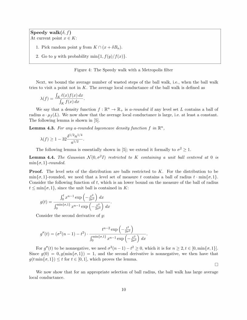
Speedy walk(δ, f)At current point x ∈ K:

1. Pick random point y from K ∩ (x+ δBn).

2. Go to y with probability min1, f(y)/f(x).

Figure 4: The Speedy walk with a Metropolis filter

Next, we bound the average number of wasted steps of the ball walk, i.e., when the ball walktries to visit a point not in K. The average local conductance of the ball walk is defined as

λ(f) =

∫K `(x)f(x) dx∫K f(x) dx

.

We say that a density function f : Rn → R+ is a-rounded if any level set L contains a ball ofradius a · µf (L). We now show that the average local conductance is large, i.e. at least a constant.The following lemma is shown in [5].

Lemma 4.3. For any a-rounded logconcave density function f in Rn,

λ(f) ≥ 1− 32δ1/2n1/4

a1/2.

The following lemma is essentially shown in [5]; we extend it formally to σ2 ≥ 1.

Lemma 4.4. The Gaussian N (0, σ2I) restricted to K containing a unit ball centered at 0 isminσ, 1-rounded.

Proof. The level sets of the distribution are balls restricted to K. For the distribution to beminσ, 1-rounded, we need that a level set of measure t contains a ball of radius t · minσ, 1.Consider the following function of t, which is an lower bound on the measure of the ball of radiust ≤ minσ, 1, since the unit ball is contained in K:

g(t) =

∫ t0 x

n−1 exp(− x2

2σ2

)dx∫ minσ,1

0 xn−1 exp(− x2

2σ2

)dx.

Consider the second derivative of g:

g′′(t) = (σ2(n− 1)− t2) ·tn−2 exp

(− t2

2σ2

)∫ minσ,1

0 xn−1 exp(− x2

2σ2

)dx.

For g′′(t) to be nonnegative, we need σ2(n− 1)− t2 ≥ 0, which it is for n ≥ 2, t ∈ [0,minσ, 1].Since g(0) = 0, g(minσ, 1) = 1, and the second derivative is nonnegative, we then have thatg(tminσ, 1) ≤ t for t ∈ [0, 1], which proves the lemma.

We now show that for an appropriate selection of ball radius, the ball walk has large averagelocal conductance.

10

Lemma 4.5. If δ ≤ minσ, 1/(4096√n), then the average local conductance, λ(f), for the density

function f proportional to the Gaussian N (0, σ2In) restricted to K containing the unit ball, is atleast 1/2.

Proof. Using Lemma 4.3 and Lemma 4.4, we have that

λ(f) ≥ 1− 32minσ1/2, 1n1/4

64n1/4 minσ1/2, 1=

1

2.

The following lemma is shown in [5].

Lemma 4.6. If the average local conductance is at least λ, M(Q0, Q) ≤ M , and the speedy walktakes t steps, then the expected number of steps of the corresponding ball walk is at most Mt/λ.

We can now prove Theorem 3.3.Proof. (of Theorem 3.3) By Theorem 4.2 and Theorem 4.1, we have selecting δ =minσ, 1/(4096

√n) implies that the speedy walk starting from a distribution that is M -warm

will be within total variation distance ε of the target distribution in O(maxσ2, 1n2 log(M/ε))steps.

By Lemma 4.6, the ball walk will, in expectation, take at most 2M times as many steps sincethe average local conductance λ is at least 1/2. We then run the ball walk for log(1/p) times asmany steps, which gives that the ball walk will be within ε total variation distance with probabilityat least 1− p.

We can now prove Theorem 1.2 (note we are analyzing only the sampling phases of Figure 2).Proof. (of Theorem 1.2) First we bound the total number of sampling phases of Figure 2. Thevariance starts at 1/(4n) and cools at a rate of 1+1/n until it equals 8C2. Thus, there are O(n log n)phases here, assuming that C = poly(n). Then, the cooling rate changes to 1 + σ2/(C2n) until thevariance equals C2n. Observe that it will take O(n) phases to increase the variance to 16C2. It willtake roughly 1/4 as many phases until the variance reaches 32C2, so by bounding by a geometricseries we see that the total number of phases here is O(n). Therefore, the total number of samplingphases is O(n log n). To get an overall sampling failure probability of p, we allot O(p/(n log n))failure probability to each phase. Also note that we set the target total variation distance of eachphase to be O(ε/(n log n)).

Next note that the sampler will always have a warm start, in fact the warmness will be boundedby√e. For the phases when the cooling rate is 1+1/n, we use Lemma 5.9 of [5]. When the cooling

rate is 1 + σ2/(C2n), we use Lemma 3.2.Finally, we bound the complexity of each sampling phase. We see that when σ2 ≤ 8C2

that the mixing time of each phase is O(C2n2), thus the total number of ball walk steps isO(C2n3 log n log n/ε log n/p). Then, when the cooling rate becomes 1 + σ2/(C2n), group thephases into chunks where each chunk increase the variance by a factor of 2. Consider a chunkthat starts with variance σ2. The chunk will consist of O(C2n/σ2) phases, each of which has mix-ing time O(σ2n2 log n/ε log n/p). Since there will be O(log n) chunks, the total mixing time of achunk is O(C2n3 log n log n/ε log n/p). Thus the total mixing time of all the sampling phases isO(C2n3 log n log n/ε log n/p).

11

4.2 Variance of the ratio estimator

The goal of this section is to prove the Lemma 3.1, which gives a bound on the variance of therandom variable we use to estimate the ratio of Gaussian integrals in the volume algorithm inFigure 2. We use the Localization Lemma in [15], which allows us to reduce inequalities in Rn to1-dimensional inequalities on needles. A needle N is defined as an interval I = [a, b] in Rn alongwith a nonnegative linear function on I.

Lemma 4.7. Let f1, f2, f3, f4 : Rn → R be nonnegative continuous functions, and β, γ > 0. Thenthe following are equivalent:

1. For every convex body K ⊆ Rn,(∫Kf1

)β (∫Kf2

)γ≤(∫

Kf3

)β (∫Kf4

)γ.

2. For every needle N ⊆ Rn,(∫Nf1

)β (∫Nf2

)γ≤(∫

Nf3

)β (∫Nf4

)γ.

For our particular functions, we can simplify the integrals in the inequality over all needlescontained in R · Bn. The following lemma says that if Equation 4 holds for some value c, thenLemma 3.1 holds for the same value c.

Lemma 4.8. If for all intervals [`, u] ⊆ [−1, 1] and b > −`,∫ u` (t+ b)n−1 exp

(− (1+α)t2R2

2σ2

)dt∫ u` (t+ b)n−1 exp

(− (1−α)t2R2

2σ2

)dt(∫ u

` (t+ b)n−1 exp(− t2R2

2σ2

)dt)2 ≤ c

for some c ∈ R, then for all convex bodies K ⊆ R ·Bn,

F ( σ2

1+α)F ( σ2

1−α)

F (σ2)2≤ c.

We defer the proof of Lemma 4.8 to the end of the section. We now describe how we useLemma 4.8 to prove the variance bound. For convenience, we now assume K is contained in a ballof radius

√n, i.e. we set R =

√n, and then later extend the analysis to any R. Define

g(σ2, b, t) := (t+ b)n−1 exp

(− t

2n

2σ2

)(1)

for b ≥ −`, σ2 > 0. Also, define a restriction of g to an interval [`, u]:

g[`,u](σ2, b, t) =

(t+ b)n−1 exp

(− t2n

2σ2

)if t ∈ [`, u]

0 otherwise

As a function of t, both g and g[`,u] are logconcave, as they are the product of logconcave functions.Therefore they have a unique maximum value, and moreover the maximum achieved at a singlepoint.

To bound the variance ratio, we will establish bounds on each of the three integrals. For eachintegral we bound the maximum of its integrand, then use logconcavity to bound the integral.

12

Lemma 4.9. Let h : R → R+ be a logconcave function with maximum Mh = h(y∗) and δ be suchthat maxh(y∗ + δ), h(y∗ − δ) = Mh/2. Then,

δMh

2≤∫Rg(x) dx ≤ 4δMh.

Proof. The first inequality is clear since there at least one of y∗+ δ and y∗− δ achieves Mh/2 andtherefore h has value at least Mh/2 in an interval of length δ.

For the second inequality, we use Lemma 5.6(a) from [22]. The lemma says that for anylogconcave function h, Pr(g(x) ≤ cMh) ≤ c. Using c = 1/2, the integral of h outside the interval[y∗ − δ, y∗ + δ] is at most the integral of h inside this interval, and the latter is at most 2δMh.

Suppose that g(σ2, b, t), t ∈ R, is maximized at t∗σ2 and suppose g[`,u](σ2, b, t) is maximized at

y∗σ2 . Let M(σ2) = g(σ2, b, t∗σ2) and M[`,u](σ2) = g[`,u](σ

2, b, t∗σ2). Clearly M[`,u](σ2) ≤ M(σ2). Let

δσ2 be such that

maxg[`,u](σ

2, b, y∗σ2 − δσ2), g[`,u](σ2, b, y∗σ2 + δσ2)

= M[`,u](σ

2)/2.

Our strategy to bound the variance ratio will be to separately bound the ratio of the maximaof the integrands and the ratio of their “halving” widths, which will give a bound on the varianceratio of

64 ·M[`,u](

σ2

1+α)M[`,u](σ2

1−α)

M[`,u](σ2)2·δσ2/(1+α)δσ2/(1−α)

δσ22 .

Proof.(of Lemma 4.8)Applying Lemma 4.7 and setting f1(x) = f(σ2/(1 + α), x), f2(x) = f(σ2/(1 − α), x), f3(x) =

f4(x) =√c · f(σ2, x), β = γ = 1, we have that

F ( σ2

1+α)F ( σ2

1−α)

F (σ2)2≤ c

if and only if for all needles N ⊆ Rn,∫N f( σ2

1+α , x) dx∫N f( σ2

1−α , x) dx(∫N f(σ2, x) dx

)2 ≤ c.

To prove the lemma, we will show that we can reduce the inequality for an arbitrary needleN ⊆ Rn to the simpler form. N is defined by an interval I in Rn and a non-negative linear functionon I.

Consider Figure 5. Define z as the closest distance from the origin to the extension of the I inboth directions. Parameterize the interval I in terms of t, where t = 0 gives the closest point alongthe extension of I to the origin (note t = 0 does not necessarily have to be on I). Also define theminimum and maximum values of t on I as ` and u respectively. Note that we can assume that−R ≤ ` ≤ u ≤ R since f is 0 outside of R ·Bn. We then have that∫Nf(σ2, x) dx =

∫ u

`(mt+b)n−1 exp

(− t

2 + z2

2σ2

)) dt = exp

(− z2

2σ2

)·∫ u

`(mt+b)n−1 exp

(− t2

2σ2

)dt

13

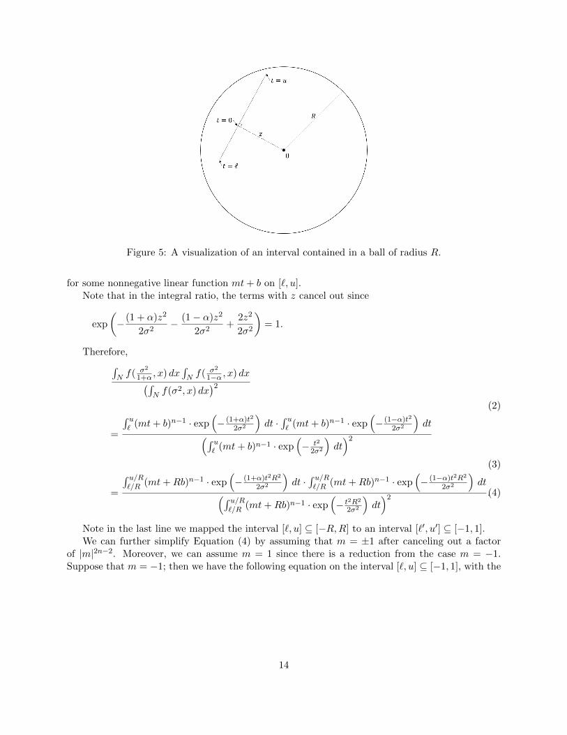
Figure 5: A visualization of an interval contained in a ball of radius R.

for some nonnegative linear function mt+ b on [`, u].Note that in the integral ratio, the terms with z cancel out since

exp

(−(1 + α)z2

2σ2− (1− α)z2

2σ2+

2z2

2σ2

)= 1.

Therefore,∫N f( σ2

1+α , x) dx∫N f( σ2

1−α , x) dx(∫N f(σ2, x) dx

)2(2)

=

∫ u` (mt+ b)n−1 · exp

(− (1+α)t2

2σ2

)dt ·

∫ u` (mt+ b)n−1 · exp

(− (1−α)t2

2σ2

)dt(∫ u

` (mt+ b)n−1 · exp(− t2

2σ2

)dt)2

(3)

=

∫ u/R`/R (mt+Rb)n−1 · exp

(− (1+α)t2R2

2σ2

)dt ·

∫ u/R`/R (mt+Rb)n−1 · exp

(− (1−α)t2R2

2σ2

)dt(∫ u/R

`/R (mt+Rb)n−1 · exp(− t2R2

2σ2

)dt)2 .(4)

Note in the last line we mapped the interval [`, u] ⊆ [−R,R] to an interval [`′, u′] ⊆ [−1, 1].We can further simplify Equation (4) by assuming that m = ±1 after canceling out a factor

of |m|2n−2. Moreover, we can assume m = 1 since there is a reduction from the case m = −1.Suppose that m = −1; then we have the following equation on the interval [`, u] ⊆ [−1, 1], with the

14

restriction that b ≥ u:∫ u` (b− y)n−1 exp

(− (1+α)y2R2

2σ2

)dy ·

∫ u` (b− y)n−1 exp

(− (1−α)y2R2

2σ2

)dy(∫ u

` (b− y)n−1 exp(−y2R2

2σ2

)dy)2

=

∫ −`−u(b+ t)n−1 exp

(− (1+α)t2R2

2σ2

)dt ·

∫ −`−u(b+ t)n−1 exp

(− (1−α)t2R2

2σ2

)dt(∫ −`

−u(b+ t)n−1 exp(− t2R2

2σ2

)dt)2 ,

where we used the substitution t = −y. This is then equivalent to the case m = 1 after mapping[−u,−`] to [`, u].

Thus we have the reduction to all needles and applying localization as in Lemma 4.7 proves thelemma.

As indicated by the statement of Lemma 3.1, we will get a bound on the variance of the ratioestimator of

F ( σ2

1+α)F ( σ2

1−α)

F (σ2)2≤ c1 exp

(c2α2R2

σ2

).

4.2.1 Locating the maxima

We begin by locating the maximum of g, as defined in (1). The maximum of g will determine themaximum of g[`,u], based on if the maximum of g is less than `, in [`, u], or greater than u.

Taking the derivative of g(σ2, b, t) = (t+ b)n−1 · exp(−nt2/(2σ2)

), we see that

d(g(σ2, b, t))

dt= (t+ b)n−2 exp

(− nt

2

2σ2

)[−nt

2

σ2− nbt

σ2+ n− 1

](5)

Therefore, the derivative equals 0 if t+b = 0 or nt2/σ2 +nbt/σ2−n+1 = 0. For t = b to equal 0, weneed that t = ` and b = −`. However, this point cannot be a local maximum of g since the derivativeis positive to the immediate right of t = `. We now consider when t2 + bt− σ2(n− 1)/n = 0:

t∗ =−b±

√b2 + 4σ2(n− 1)/n

2

=b

2

(−1 +

√1 +

4σ2(n− 1)

b2n

)(6)

Note that we ignore the negative case in (6) since it would give a point < `. The function willachieve a local maximum at t∗, but t∗ is not necessarily in [`, u]. We thus have 3 cases for whereg[`,u] is maximized:

• t∗ ∈ [`, u] and the unique maximum is t∗.

15

• t∗ < `: the function is strictly decreasing on [`, u] and the unique maximum is `.

• t∗ > u: the function is strictly increasing on [`, u] and the unique maximum is u.

The following lemma allows us to restrict the range of b-values when the maximum is in [−1, 1]and is helpful for bounding the ratio of maxima in the next section.

Lemma 4.10. If σ2 ≥ 8, n ≥ 10, and t∗σ2 ∈ [−1, 1], then b ≥ 3σ2/4.

Proof. We have that

t∗σ2 =−b+

√b2 + 4σ2(n−1)

n

2≥−b+

√b2 + 18σ2

5

2.

Thus we need that b2 + 18σ2/5 < (b+ 2)2 to have t∗σ2 ≤ 1, which implies that

4b+ 4 ≥ 18σ2

5⇒ b

σ2≥ 18− 20/σ2

20≥ 18− 5/2

20=

31

40>

3

4.

4.2.2 Bounding ratio of maxima

In this section, we prove the following lemma.

Lemma 4.11. Suppose that σ2 ≥ 8, α ≤ 1/10, and n ≥ 10. Then the ratio

M[`,u](σ2

1+α)M[`,u](σ2

1−α)

M[`,u](σ2)≤ exp

(7α2n

σ2

).

Our first goal is to get a worst-case bound on the ratio

M[`,u](σ2

1+α)M[`,u](σ2

1−α)

M[`,u](σ2)2

assuming that t∗σ2 ∈ [`, u], and then we show that the ratio will only decrease when t∗σ2 /∈ [`, u].

Lemma 4.12. Suppose that t∗σ2 ∈ [`, u] ⊆ [−1, 1], σ2 ≥ 8, α ≤ 1/10, and n ≥ 10. Then

M[`,u](σ2

1+α)M[`,u](σ2

1−α)

M[`,u](σ2)2≤ exp

(7α2n

σ2

).

Proof. Note that it is sufficient to consider the case when t∗σ2/(1+α), t∗σ2/(1−α) ∈ [`, u] since the

maxima only decrease when g is restricted to the interval [`, u]. We thus have that

M[`,u](σ2

1+α)M[`,u](σ2

1−α)

M[`,u](σ2)2≤g( σ2

1+α , b, t∗σ2/(1+α)) · g( σ2

1−α , b, t∗σ2/(1−α))

g(σ2, b, t∗σ2)2

=

((b+ t∗σ2/(1+α))(b+ t∗σ2/(1−α))

(b+ t∗σ2)2

)n−1

. . .

. . . · exp( n

2σ2

(2t∗σ2

2 − (1 + α)t∗σ2/(1+α)2 − (1− α)t∗σ2/(1−α)

2))

. (7)

16

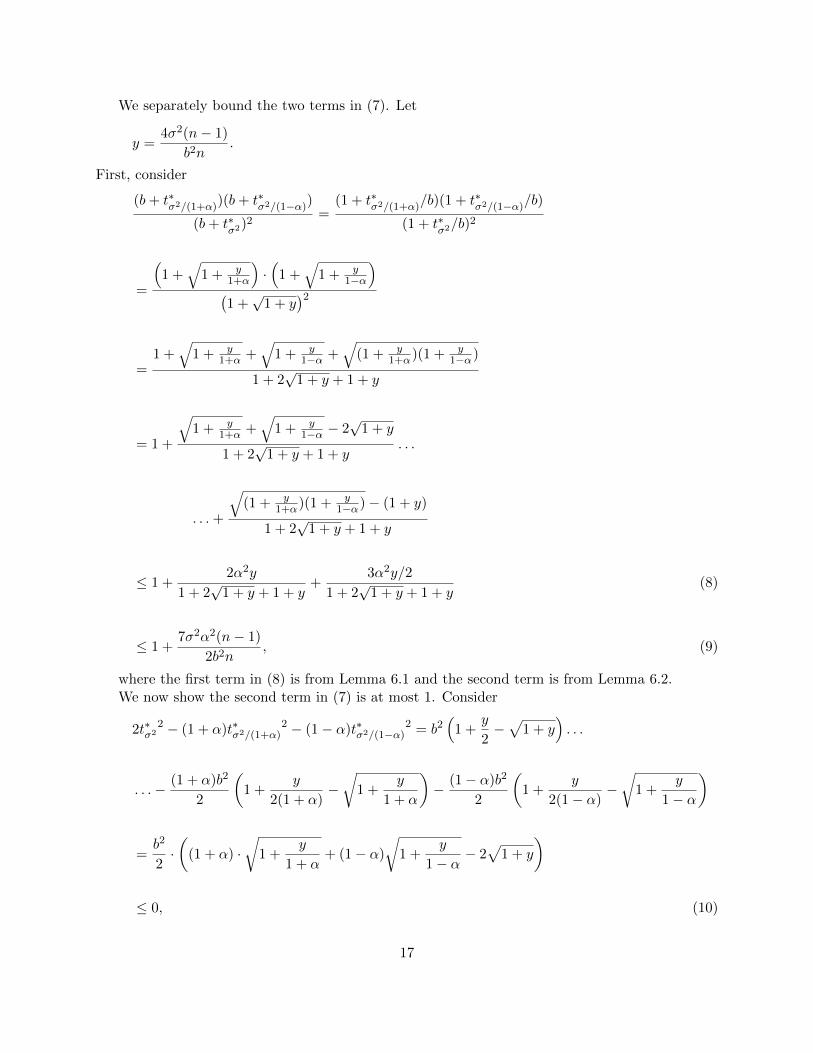
We separately bound the two terms in (7). Let

y =4σ2(n− 1)

b2n.

First, consider

(b+ t∗σ2/(1+α))(b+ t∗σ2/(1−α))

(b+ t∗σ2)2

=(1 + t∗σ2/(1+α)/b)(1 + t∗σ2/(1−α)/b)

(1 + t∗σ2/b)2

=

(1 +

√1 + y

1+α

)·(

1 +√

1 + y1−α

)(1 +√

1 + y)2

=1 +

√1 + y

1+α +√

1 + y1−α +

√(1 + y

1+α)(1 + y1−α)

1 + 2√

1 + y + 1 + y

= 1 +

√1 + y

1+α +√

1 + y1−α − 2

√1 + y

1 + 2√

1 + y + 1 + y. . .

. . .+

√(1 + y

1+α)(1 + y1−α)− (1 + y)

1 + 2√

1 + y + 1 + y

≤ 1 +2α2y

1 + 2√

1 + y + 1 + y+

3α2y/2

1 + 2√

1 + y + 1 + y(8)

≤ 1 +7σ2α2(n− 1)

2b2n, (9)

where the first term in (8) is from Lemma 6.1 and the second term is from Lemma 6.2.We now show the second term in (7) is at most 1. Consider

2t∗σ22 − (1 + α)t∗σ2/(1+α)

2 − (1− α)t∗σ2/(1−α)2 = b2

(1 +

y

2−√

1 + y). . .

. . .− (1 + α)b2

2

(1 +

y

2(1 + α)−√

1 +y

1 + α

)− (1− α)b2

2

(1 +

y

2(1− α)−√

1 +y

1− α

)

=b2

2·(

(1 + α) ·√

1 +y

1 + α+ (1− α)

√1 +

y

1− α− 2√

1 + y

)

≤ 0, (10)

17

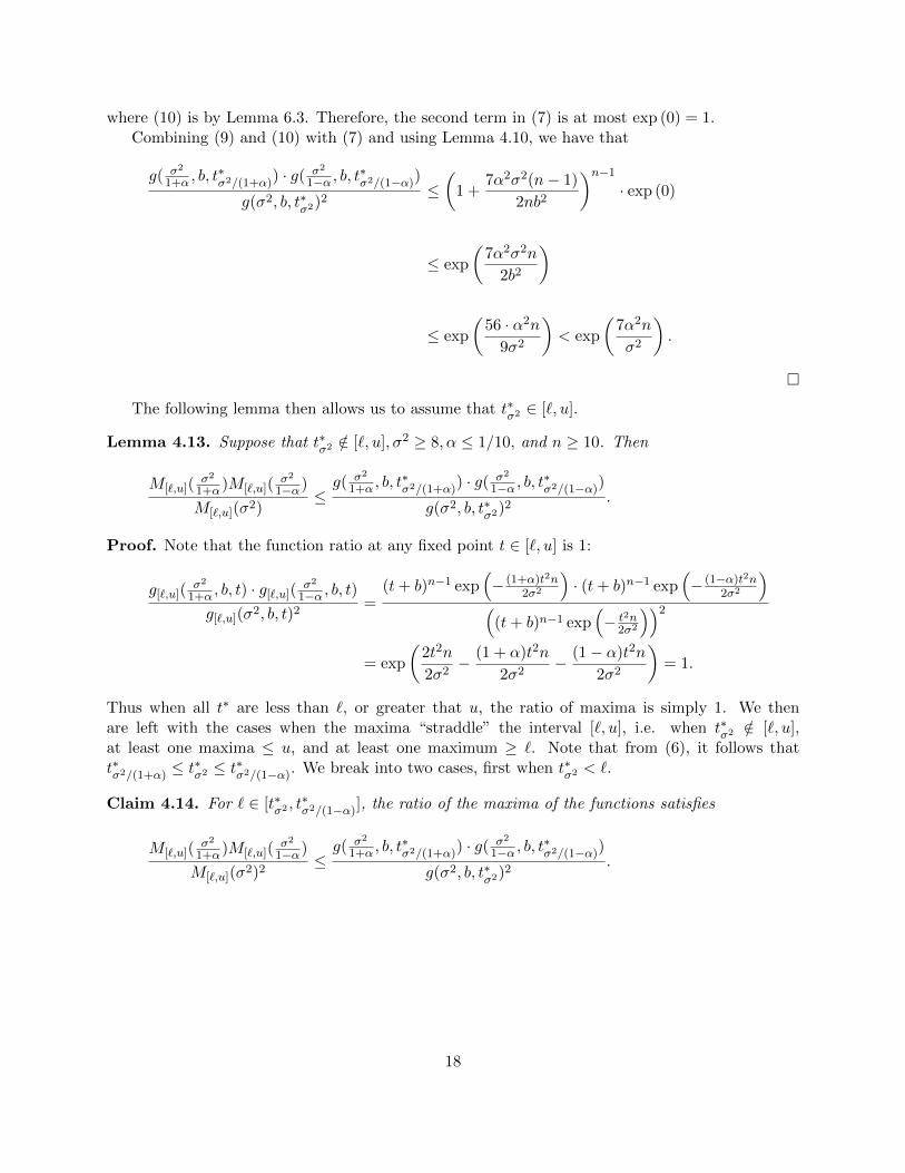
where (10) is by Lemma 6.3. Therefore, the second term in (7) is at most exp (0) = 1.Combining (9) and (10) with (7) and using Lemma 4.10, we have that

g( σ2

1+α , b, t∗σ2/(1+α)) · g( σ2

1−α , b, t∗σ2/(1−α))

g(σ2, b, t∗σ2)2

≤(

1 +7α2σ2(n− 1)

2nb2

)n−1

· exp (0)

≤ exp

(7α2σ2n

2b2

)

≤ exp

(56 · α2n

9σ2

)< exp

(7α2n

σ2

).

The following lemma then allows us to assume that t∗σ2 ∈ [`, u].

Lemma 4.13. Suppose that t∗σ2 /∈ [`, u], σ2 ≥ 8, α ≤ 1/10, and n ≥ 10. Then

M[`,u](σ2

1+α)M[`,u](σ2

1−α)

M[`,u](σ2)≤g( σ2

1+α , b, t∗σ2/(1+α)) · g( σ2

1−α , b, t∗σ2/(1−α))

g(σ2, b, t∗σ2)2

.

Proof. Note that the function ratio at any fixed point t ∈ [`, u] is 1:

g[`,u](σ2

1+α , b, t) · g[`,u](σ2

1−α , b, t)

g[`,u](σ2, b, t)2=

(t+ b)n−1 exp(− (1+α)t2n

2σ2

)· (t+ b)n−1 exp

(− (1−α)t2n

2σ2

)(

(t+ b)n−1 exp(− t2n

2σ2

))2

= exp

(2t2n

2σ2− (1 + α)t2n

2σ2− (1− α)t2n

2σ2

)= 1.

Thus when all t∗ are less than `, or greater that u, the ratio of maxima is simply 1. We thenare left with the cases when the maxima “straddle” the interval [`, u], i.e. when t∗σ2 /∈ [`, u],at least one maxima ≤ u, and at least one maximum ≥ `. Note that from (6), it follows thatt∗σ2/(1+α) ≤ t

∗σ2 ≤ t∗σ2/(1−α). We break into two cases, first when t∗σ2 < `.

Claim 4.14. For ` ∈ [t∗σ2 , t∗σ2/(1−α)], the ratio of the maxima of the functions satisfies

M[`,u](σ2

1+α)M[`,u](σ2

1−α)

M[`,u](σ2)2≤g( σ2

1+α , b, t∗σ2/(1+α)) · g( σ2

1−α , b, t∗σ2/(1−α))

g(σ2, b, t∗σ2)2

.

18

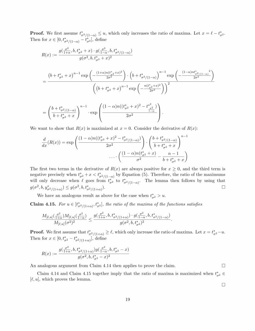
Proof. We first assume t∗σ2/(1−α) ≤ u, which only increases the ratio of maxima. Let x = `− t∗σ2 .

Then for x ∈ [0, t∗σ2/(1−α) − t∗σ2 ], define

R(x) :=g( σ2

1+α , b, t∗σ2 + x) · g( σ2

1−α , b, t∗σ2/(1−α))

g(σ2, b, t∗σ2 + x)2

=

(b+ t∗σ2 + x

)n−1exp

(−

(1+α)n(t∗σ2

+x)2

2σ2

)·(b+ t∗σ2/(1−α)

)n−1exp

(−

(1−α)nt∗σ2/(1−α)

2

2σ2

)((b+ t∗

σ2 + x)n−1

exp

(−n(t∗

σ2+x)2

2σ2

))2

=

(b+ t∗σ2/(1−α)

b+ t∗σ2 + x

)n−1

· exp

(1− α)n((t∗σ2 + x)2 − t∗2σ2

1−α)

2σ2

.

We want to show that R(x) is maximized at x = 0. Consider the derivative of R(x):

d

dx(R(x)) = exp

((1− α)n((t∗σ2 + x)2 − t∗σ2/(1−α))

2σ2

)·

(b+ t∗σ2/(1−α)

b+ t∗σ2 + x

)n−1

. . . ·(

(1− α)n(t∗σ2 + x)

σ2− n− 1

b+ t∗σ2 + x

)The first two terms in the derivative of R(x) are always positive for x ≥ 0, and the third term isnegative precisely when t∗σ2 +x < t∗σ2/(1−α) by Equation (5). Therefore, the ratio of the maximums

will only decrease when ` goes from t∗σ2 to t∗σ2/(1−α). The lemma then follows by using that

g(σ2, b, y∗σ2/(1+α)) ≤ g(σ2, b, t∗σ2/(1+α)).

We have an analogous result as above for the case when t∗σ2 > u.

Claim 4.15. For u ∈ [t∗σ2/(1+α), t∗σ2 ], the ratio of the maxima of the functions satisfies

M[`,u](σ2

1+α)M[`,u](σ2

1−α)

M[`,u](σ2)2≤g( σ2

1+α , b, t∗σ2/(1+α)) · g( σ2

1−α , b, t∗σ2/(1−α))

g(σ2, b, t∗σ2)2

.

Proof. We first assume that t∗σ2/(1+α) ≥ `, which only increase the ratio of maxima. Let x = t∗σ2−u.

Then for x ∈ [0, t∗σ2 − t∗σ2/(1+α)], define

R(x) :=g( σ2

1+α , b, t∗σ2/(1+α))g( σ2

1−α , b, t∗σ2 − x)

g(σ2, b, t∗σ2 − x)2

An analogous argument from Claim 4.14 then applies to prove the claim.

Claim 4.14 and Claim 4.15 together imply that the ratio of maxima is maximized when t∗σ2 ∈[`, u], which proves the lemma.

19

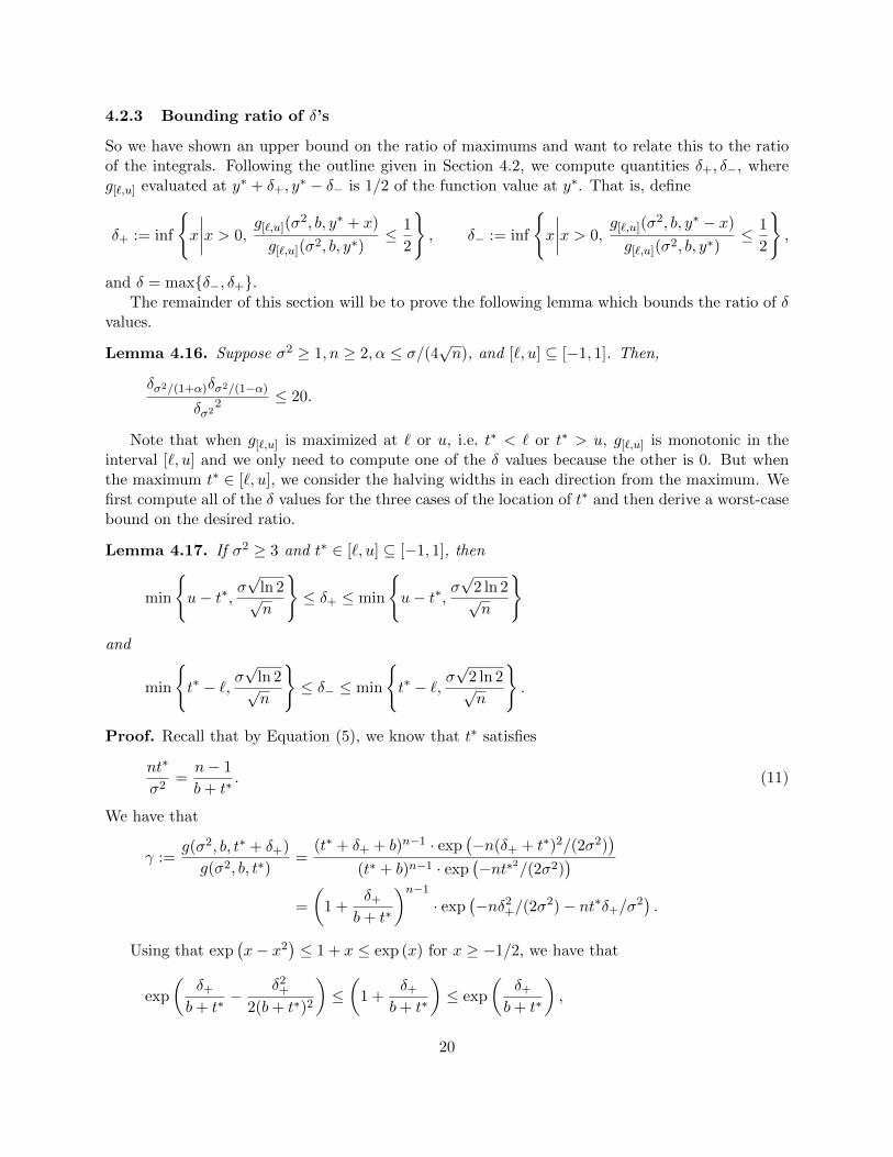
4.2.3 Bounding ratio of δ’s

So we have shown an upper bound on the ratio of maximums and want to relate this to the ratioof the integrals. Following the outline given in Section 4.2, we compute quantities δ+, δ−, whereg[`,u] evaluated at y∗ + δ+, y

∗ − δ− is 1/2 of the function value at y∗. That is, define

δ+ := inf

x

∣∣∣∣x > 0,g[`,u](σ

2, b, y∗ + x)

g[`,u](σ2, b, y∗)≤ 1

2

, δ− := inf

x

∣∣∣∣x > 0,g[`,u](σ

2, b, y∗ − x)

g[`,u](σ2, b, y∗)≤ 1

2

,

and δ = maxδ−, δ+.The remainder of this section will be to prove the following lemma which bounds the ratio of δ

values.

Lemma 4.16. Suppose σ2 ≥ 1, n ≥ 2, α ≤ σ/(4√n), and [`, u] ⊆ [−1, 1]. Then,

δσ2/(1+α)δσ2/(1−α)

δσ22 ≤ 20.

Note that when g[`,u] is maximized at ` or u, i.e. t∗ < ` or t∗ > u, g[`,u] is monotonic in theinterval [`, u] and we only need to compute one of the δ values because the other is 0. But whenthe maximum t∗ ∈ [`, u], we consider the halving widths in each direction from the maximum. Wefirst compute all of the δ values for the three cases of the location of t∗ and then derive a worst-casebound on the desired ratio.

Lemma 4.17. If σ2 ≥ 3 and t∗ ∈ [`, u] ⊆ [−1, 1], then

min

u− t∗, σ

√ln 2√n

≤ δ+ ≤ min

u− t∗, σ

√2 ln 2√n

and

min

t∗ − `, σ

√ln 2√n

≤ δ− ≤ min

t∗ − `, σ

√2 ln 2√n

.

Proof. Recall that by Equation (5), we know that t∗ satisfies

nt∗

σ2=n− 1

b+ t∗. (11)

We have that

γ :=g(σ2, b, t∗ + δ+)

g(σ2, b, t∗)=

(t∗ + δ+ + b)n−1 · exp(−n(δ+ + t∗)2/(2σ2)

)(t∗ + b)n−1 · exp

(−nt∗2/(2σ2)

)=

(1 +

δ+

b+ t∗

)n−1

· exp(−nδ2

+/(2σ2)− nt∗δ+/σ

2).

Using that exp(x− x2

)≤ 1 + x ≤ exp (x) for x ≥ −1/2, we have that

exp

(δ+

b+ t∗−

δ2+

2(b+ t∗)2

)≤(

1 +δ+

b+ t∗

)≤ exp

(δ+

b+ t∗

),

20

and therefore we have an upper bound on the function ratio of

γ ≤ exp

(−δ+(

nt∗

σ2− n− 1

b+ t∗)−

nδ2+

2σ2

)= exp

(−nδ2

+

2σ2

)and the lower bound of

γ ≥ exp

(−δ+

(nt∗

σ2− n− 1

b+ t∗

)− δ2

+

(n

2σ2+

n− 1

(b+ t∗)2

))= exp

(−δ2

+

(n

2σ2+

n− 1

(b+ t∗)2

))= exp

(−δ2

+

(n

2σ2+

n2t∗2

σ4(n− 1)

))by Equation (11)

= exp

(−δ2

+n

2σ2(1 +

2nt∗2

σ2(n− 1))

)

≥ exp

(−δ2

+n

σ2

).

We are searching for the range of δ+’s which could make γ equal 1/2. From the two boundsabove, solving for δ+ in

exp

(−nδ2

+

2σ2

)=

1

2

gives an upper bound and

exp

(−δ2

+n

σ2

)=

1

2

gives a lower bound, assuming that t∗+ δ+ ≤ u. Note that both bounds above only have δ2+ terms,

so this bound also applies to δ− if t∗ − δ− ≥ `. If shifting by δ goes outside the interval, e.g.t∗ + δ+ > u, then we shorten the width to be the distance from t∗ to the interval endpoint.

We now handle the cases when t∗ lies outside the interval [`, u]; first consider when t∗ < `.

Lemma 4.18. If t∗ < `, σ2 ≥ 1, n ≥ 2, then

min

σ

3√n,

1

2n(`/σ2 − 1/(b+ `)), u− `

≤ δ ≤ min

σ√

2√n,

1

n(`/σ2 − 1/(b+ `)), u− `

.

Proof. Recall that t∗ satisfies

nt∗

σ2=n− 1

b+ t∗,

21

which implies that

n`

σ2>n− 1

b+ `

since t∗ < `. We have that

g(σ2, b, `+ δ)

g(σ2, b, `)=

(1 +

δ

b+ `

)n−1

· exp

(−nδ

2

2σ2− n`δ

σ2

).

Using that exp(x− x2/2) ≤ 1 + x ≤ exp(x), we have that

g(σ2, b, `+ δ)

g(σ2, b, `)≤ exp

(−nδ

2

2σ2− δ

(n`

σ2− n− 1

b+ `

))and

g(σ2, b, `+ δ)

g(σ2, b, `)≥ exp

(−δ2(

n

2σ2+

n− 1

2(b+ `)2)− δ(n`

σ2− n− 1

b+ `)

)≥ exp

(−δ2(

n

2σ2+

n2`2

2σ4(n− 1))− δ(n`

σ2− n− 1

b+ `)

)≥ exp

(−nδ

2

σ2− δ(n`

σ2− n− 1

b+ `)

),

where the last line used that σ2 ≥ 1, n ≥ 2. Suppose we set

min

c1σ√n,

c2

n(`/σ2 − 1/(b+ `))

≤ δ ≤ min

c3σ√

2√n

,c4

n(`/σ2 − 1/(b+ `))

.

Then by Lemma 6.4, we have that

exp(−c2

1 − c2

)≤ g(σ2, b, `+ δ)

g(σ2, b, `)≤ exp

(−minc2

3, c4).

We turn the above bounds on the function value at ` + δ into a range of δ values as follows.When exp

(−c2

3 − c4

)≤ 1/2, we know that the actual δ is less than this value (analogously when

exp(−minc2

1, c2)≥ 1/2, we know δ is greater than this). So we have that selecting c1, c2, c3, c4

such that

c21 + c2 ≤ ln 2 and minc2

3, c4 ≥ ln 2

gives a bound on the value of δ.Thus we can select c1 = 1/3, c2 = 1/2, c3 = 1, c4 = 1. This then implies the lemma after

handling the case when u− ` is less than δ.

By a similar argument, we get the following bounds for when t∗ > u.

Lemma 4.19. If t∗ > u and σ2 ≥ 1/2, then

min

σ

2√n,

1

2n(2/(b+ u)− u/σ2), u− `

≤ δ ≤ min

σ√

2√n,

1

n(1/(b+ u)− u/σ2), u− `

.

22

Proof. Recall that t∗ satisfies

nt∗

σ2=n− 1

b+ t∗,

which implies that

nu

σ2<n− 1

b+ u

since t∗ > u.We have that

g(σ2, b, u− δ)g(σ2, b, u)

=

(1− δ

b+ u

)n−1

· exp(−nδ2/(2σ2) + nuδ/σ2

).

Note that once δ > b+ u, the function value will be negative. Therefore, we know that

b+ u ≥ δ,

and furthermore, for our selection of δ, we have that

δ

b+ u≤ 1

(b+ u) · 2n(1/(b+ u)− u/σ2)=

1

2(n− nu(b+ u)/σ2)<

1

2(n− (n− 1))=

1

2

Using that exp(x− x2) ≤ 1 + x ≤ exp(x) for x ≥ −1/2, we have that

g(σ2, b, u− δ)g(σ2, b, u)

≤ exp

(−nδ2/(2σ2)− δ(n− 1

b+ u− nu/σ2)

),

and

g(σ2, b, u− δ)g(σ2, b, u)

≥ exp

(−δ2(n/(2σ2) +

n− 1

(b+ u)2)− δ(n− 1

b+ u− nu/σ2)

)≥ exp

(−δ2n/(2σ2)− δ(2(n− 1)

b+ u− nu/σ2)

).

Suppose we set

min

c1σ√

2√n

,c2

n(2/(b+ u)− u/σ2)

≤ δ ≤ min

c3σ√

2√n

,c4

n(1/(b+ u)− u/σ2)

.

Then by Lemma 6.4, we have that

exp(−c2

1 − c2

)≤ g(σ2, b, u− δ)

g(σ2, b, `)≤ exp

(−minc2

3, c4).

Thus when exp(−c2

3 − c4

)≤ 1/2, we know that the actual δ is less than this value (analogously

when exp(−minc2

1, c2)≥ 1/2, we know δ is greater than this). So we have that selecting

c1, c2, c3, c4 such that

c21 + c2 ≤ ln 2 and minc2

3, c4 ≥ ln 2

23

gives a bound on the value of δ.Thus we can select c1 = 1/(2

√2), c2 = 1/2, c3 = 1, c4 = 1. This then implies the lemma after

handling the case when u− ` is less than δ.

Now that we have derived all the δ values, the following three claims will bound the δ-ratio indifferent cases and together prove Lemma 4.16.

Claim 4.20. For [`, u] ⊆ [−1, 1], suppose that t∗σ2/(1+α) ≤ u, t∗σ2/(1−α) ≥ `, and α ≤ σ/(4√n).

Then

δσ2/(1+α)δσ2/(1−α)

δσ22 ≤ 20.

Proof. The following claim essentially says that if t∗σ2 < ` ≤ t∗σ2/(1−α), then δσ2 behaves as if

t∗σ2 ∈ [`, u].

Claim 4.21. For t∗σ2 < ` ≤ t∗σ2/(1−α), u ≤ 1, and α ≤ σ/(c√n), we have that

1

n`/σ2 − (n− 1)/(b+ `)≥ cσ

2√n.

Proof. It suffices to prove the lemma for ` = t∗σ2/(1−α), i.e. show that

1

nt∗σ2/(1−α)

/σ2 − (n− 1)/(b+ t∗σ2/(1−α)

)≥ cσ

2√n,

since the quantity is monotonically decreasing with `.We have that

t∗σ2/(1−α)2+bt∗σ2/(1−α) −

σ2(n− 1)

n. . .

=

(b2

4− b2

2·

√1 +

4σ2(n− 1)

(1− α)nb2+b2

4· (1 +

4σ2(n− 1)

(1− α)nb2)

)

. . .+

(−b2

2+b2

2·

√1 +

4σ2(n− 1)

(1− α)nb2

)− σ2(n− 1)

n

=σ2(n− 1)

(1− α)n− σ2(n− 1)

n=σ2(n− 1)α

(1− α)n

≤ 3ασ2

2.

24

Thus

1

nt∗σ2/(1−α)

/σ2 − (n− 1)/(b+ t∗σ2/(1−α)

)≥

2(b+ t∗σ2/(1−α))

3nα

≥ 2bc√n

3σn

≥ cσ

2√n,

where we used the fact that b/σ ≥ 3σ/4 from Lemma 4.10.

We have a symmetric claim for when t∗σ2 > u whose proof is nearly identical.

Claim 4.22. For t∗σ2 > u, t∗σ2/(1+α) ≤ u, u ≤ 1, and α ≤ σ/(c√n), we have that

1

(n− 1)/(b+ u)− nu/σ2≥ cσ

2√n.

We break into cases for the value of δσ2 . By Claim 4.21 and Claim 4.22, we can restrict ourselvesto δσ2 = Ω(σ/

√n) or Ω(u − `). More precisely, by also applying Lemmas 4.17, 4.18, and 4.19, we

know that either δσ2 ≥ σ√

1/(3n) or δσ2 ≥ (u− `)/2.

• Case 1:

δσ2 ≥ σ√

1

3n.

Then Lemmas 4.17, 4.18, and 4.19,

δσ2/(1+α)δσ2/(1−α)

δσ22 ≤ 18

√1

1 + α· 1

1− α< 20.

• Case 2:

σ√

1/(3n) ≥ δσ2 ≥ (u− `)/2.

Since δσ2/(1+α), δσ2/(1−α) ≤ u− `,

δσ2/(1+α)δσ2/(1−α)

δσ22 ≤ (u− `) · (u− `)

(u− `)2/4≤ 4.

We then bound the ratio of the δ values for the two remaining cases, all t∗ < ` and all t∗ > u.

Claim 4.23. If t∗σ2/(1+α), t∗σ2 , t

∗σ2/(1−α) < ` ≤ 1, σ2 ≥ 1, n ≥ 2, and α ≤ σ/(4

√n),

δσ2/(1+α)δσ2/(1−α)

δσ22 ≤ 20.

25

Proof. We break into three cases.Case 1:

δσ2 ≥ σ√

1

3n.

Then by Lemma 4.18,

δσ2/(1+α)δσ2/(1−α)

δσ22 ≤

18√

(1 + α)/(1− α)

1 + α

< 20.

Case 2:

σ

√1

3n> δσ2 ≥

1

2n(`/σ2 − 1/(b+ `)).

Then,

δσ2/(1+α)δσ2/(1−α)

δσ22 ≤

4(`/σ2 − 1/(b+ `)

)2((1 + α)`/σ2 − 1/(b+ `)) · ((1− α)`/σ2 − 1/(b+ `))

=4(`/σ2 − 1/(b+ `))2

(`/σ2 − 1/(b+ `) + α`/σ2) · (`/σ2 − 1/(b+ `)− α`/σ2)

=4(`/σ2 − 1/(b+ `))2

(`/σ2 − 1/(b+ `))2 − α2`2/σ4

≤ 36/(4σ2n)

9/(4σ2n)− 1/(16σ2n)< 5,

where the last line used that `/σ2 − 1/(b+ `) ≥ 3/(2σ√n) and α ≤ σ/(4

√n).

Case 3: δσ2 = u− `.We have that δσ2/(1+α), δσ2/(1−α) ≤ u− `, and thus

δσ2/(1+α)δσ2/(1−α)

δσ22 ≤ 1.

The proof for bounding the δ-ratio for all t∗ > u is nearly identical.

Claim 4.24. If t∗σ2/(1+α), t∗σ2 , t

∗σ2/(1−α) > u, u ≤ 1, σ2 ≥ 1/2, and α ≤ σ/(4

√n), then

δσ2/(1+α)δσ2/(1−α)

δσ22 ≤ 10.

Proof. We break into three cases.Case 1:

δσ2 ≥σ

2

√1

n.

26

Then by Lemma 4.18,

δσ2/(1+α)δσ2/(1−α)

δσ22 ≤ 8

√1

1 + α· 1

1− α< 10.

Case 2:

σ

2

√1

n> δσ2 ≥

1

2n(2/(b+ u)− u/σ2).

Then,

δσ2/(1+α)δσ2/(1−α)

δσ22 ≤

4(2/(b+ u)− u/σ2

)2(2/(b+ u)− (1 + α)u/σ2) · (2/(b+ u)− (1− α)u/σ2)

=4(2/(b+ u)− u/σ2)2

(2/(b+ u)− u/σ2 − αu/σ2) · (2/(b+ u)− u/σ2 + αu/σ2)

=4(2/(b+ u)− u/σ2)2

(2/(b+ u)− u/σ2)2 − α2u2/σ4

≤ 4/(σ2n)

1/(σ2n)− 1/(16σ2n)< 5,

where the last line used that 2/(b+ u)− u/σ2 ≥ 1/(σ√n) and α ≤ σ/(4

√n).

Case 3: δσ2 = u− `.We have that δσ2/(1+α), δσ2/(1−α) ≤ u− `, and thus

δσ2/(1+α)δσ2/(1−α)

δσ22 ≤ 1.

Lemma 4.16 then follows immediately from Claims 4.20, 4.23, and 4.24.

4.2.4 Variance bound

From the results of the previous sections, we can now prove Lemma 3.1.Proof.(of Lemma 3.1)

Applying Lemma 4.9 to the bound on the maximum ratio in Lemma 4.11 and the bounds

27

on the ratio δ values in Lemma 4.16, we have that∫R g[`,u](

σ2

1+α , b, t) dt∫R g[`,u](

σ2

1−α , b, t) dt(∫R g[`,u](σ2, b, t) dt

)2

≤ 64 ·M[`,u](

σ2

1+α)M[`,u](σ2

1−α)

M[`,u](σ2)2·δσ2/(1+α)δσ2/(1−α)

δσ22

≤ 64 · exp

(7 · α

2n

σ2

)· 20

≤ 1280 · exp

(7 · α

2n

σ2

).

Then applying localization as in Lemma 4.8, we have that for any convex body K ⊆√nBn,

F ( σ2

1+α)F ( σ2

1−α)

F (σ2)2≤ 1280 · exp

(7 · α

2n

σ2

).

We now prove the lemma by extending the above bound to K ⊆ C√nBn. Let σ = σ/C.

F ( σ2

1+α)F ( σ2

1−α)

F (σ2)2=

∫K exp

(− (1+α)x2

2σ2

)dx ·

∫K exp

(−x2(1−α)

2σ2

)dx(∫

K exp(− x2

2σ2

)dx)2

=

∫K/C exp

(− (1+α)C2t2

2σ2

)dt ·

∫K/C exp

(− t2(1−α)C2

2σ2

)dt(∫

K/C exp(− t2C2

2σ2

)dt)2

=

∫K/C exp

(− (1+α)t2

2σ2

)dt ·

∫K/C exp

(− t2(1−α)

2σ2

)dt(∫

K/C exp(− t2

2σ2

)dt)2

≤ 1280 · exp

(25 · α

2n

σ2

)= 1280 · exp

(25 · α

2nC2

σ2

).

4.3 Proof of the main theorem

In this section, we prove Theorem 1.1 by analyzing the runtime of the algorithm in Figure 2 andalso showing that the volume estimate it computes is accurate.

The following lemma from [5] says that almost all of the volume of the starting Gaussian iscontained in K

28

Lemma 4.25. If σ2 ≤ 1/(n+√

8n ln(1/ε)) and Bn ⊆ K, then∫K

exp

(−−‖x‖

2

2σ2

)dx ≥ (1− ε)

∫Rn

exp

(−−‖x‖

2

2σ2

)dx.

The following lemma is essentially shown in [5], which bounds the variance assuming a fixedcooling rate of σ2

i+1 = σ2i (1 + 1/

√n).

Lemma 4.26. Let X be a random point in K with density proportional to fi(x) = exp(−‖x‖2

2σ2i

),

σ2i+1 = σ2

i (1 + 1/√n), and Y = fi+1(X)/fi(X). Then,

E(Y 2)

E(Y )2< 8.

The following lemma is the crucial component of our improved algorithm, which bounds thevariance of our ratio estimater under a faster cooling rate. It follows immediately from Lemma 3.1.

Lemma 4.27. Suppose that K ⊆ C√nBn and σ2

i ≥ 8C2. Let X be a random point in K with

density proportional to fi(x) = exp(−‖x‖2

2σ2i

), σ2i+1 = σ2

i · (1 + σi/(4C√n)), and Y = fi+1(X)/fi(X).

Then,

E(Y 2)

E(Y )2< 211.

We now show that the volume estimate computed in Algorithm 2 is accurate. Define Ri as thei-th integral ratio, i.e.

Ri :=F (σ2

i+1)

F (σ2i )

=

∫K exp

(−‖x‖2/(2σ2

i+1))dx∫

K exp(−‖x‖2/(2σ2

i ))dx

,

and let Wi denote the estimate of the algorithm for Ri.

Lemma 4.28. With probability at least 4/5,

(1− ε)R1 . . . Rm ≤W1 . . .Wm ≤ (1 + ε)R1 . . . Rm.

Proof. Let (Xi0, X

i1, X

i2, . . . , X

iki

) be the sequence of sample points for the ith volume phase. Thedistribution of each Xi is approximately the correct distribution, but slightly off based on the errorparameter ν in each phase that bounds the total variation distance. We will define new randomvariables Xi

j that have the correct distribution for each phase.

Note that X0j would be sampled from the exact distribution, and then rejected if outside of

K. Therefore Pr(X0j = X0

j ) = 1. Suppose that the total number of sample points throughout thealgorithm is t. Using induction and the definition of total variation distance, we see that

Pr(Xji = Xj

i ,∀i, j) ≥ 1− tν

Let

Y ij =

exp

(−‖X

ij‖2

2σ2i+1

)exp

(−‖X

ij‖2

2σ2i

)29

and

Wi =1

ki

ki∑j=1

Y ij .

Note that all of the Y ij have the same expectation, and it is equal to E(Wi). Suppose that we

have E(Y ij )2) ≤ ciE(Y i

j )2, or equivalently Var(Y ij ) ≤ (ci − 1)E(Y i

j )2. Then

Var(W 2i ) =

1

k2i

ki∑j=1

Var(Y ij ) =

1

kiVar(Wi) ≤

ci − 1

k· EWi)

2. (12)

Suppose that we had independence between samples. Then, we can use Equation (12) to boundthe probability of failure. We break the analysis into two part, just as in the algorithm: whenσ2i ≤ 8C2 and when σ2

i > 8C2.When σ2

i ≤ 8C2, we cool by the rate of σ2i+1 = σ2

i (1 + 1/√n). By Lemma 4.26, we know that

when σ2i+1 = σ2

i (1 + 1/√n), E(Y j

i )2) ≤ 8E(Y ji )2. As σ2

0 = 1/(4n), we can upper bound the numberof phases m1 in this phase of the algorithm as 2

√n ln(32C2n).Then by Chebyshev’s inequality, we

have that

Pr(|W1 . . . Wm1 −R1 . . . Rm1 | ≥ε

2·R1 . . . Rm1) ≤ 4Var(W1 . . . Wm1)

ε2R21 . . . R

2m1

=28m1

k1ε2.

Thus, selecting

k1 =280m1

ε2=

560√n ln(32C2n)

ε2

implies that we are within ε/2 relative error with probability at most 1/10.When σ2

i > 8C2, the analysis is a bit more involved because of the variable cooling rate. By

Lemma 4.27, when σ2 ≥ 8C2 and σ2i+1 = σ2

i (1 + σ/(8C√n)), E(Y j

i )2) ≤ 212E(Y ji )2. We divide

the cooling schedule into “chunks”, where a chunk represents the value of the variance increase bya multiplicative factor of e. Since we stop once the variance equals C2n, we have at most log nchunks of phases, and we assign ε/(2 log n) error to each chunk. Denote the number of phases inchunk i as mi. Analogously to the above, by Chebyshev’s inequality we can select

ki =213 · 10mi log3 n

ε2

to have ε/(2 log n) relative error in each phase with probability 1/(10 log n). Note that we can easilyget an upper bound on mi. Since we cool at a rate of 1 + σ/(4C

√n), we bound mi by 8C

√n/σ

for the current variance σ2. Thus assuming independence between successive samples, for a phasewith variance σ2, we can take

220C√n log3 n

ε2 maxσ, 1

samples to prove the lemma.

30

However, subsequent samples are dependent, and we must carefully bound the dependence. Theanalysis is somewhat involved, but will follow essentially the sample template as in [21, 5] whichutilizes the following lemma to bound dependence between subsequent samples, where ν is thetarget total variation distance for each sample point. For convenience, denote the entire sequenceof t samples points used in the algorithm as (Z0, Z1, . . . , Zt−1).

Lemma 4.29. (a) For 0 ≤ i < t, the random variables Zi and Zi+1 are ν-independent, and therandom variables Zi and Zi+1 are (3ν)-independent.

(b) For 0 ≤ i < t, the random variables (Z0, . . . , Zi) and Zi+1 are (3ν)-independent.(c) For 0 ≤ i < m, the random variables W1 . . . Wi and Wi+1 are (3kmν)-independent.

We can now prove the main theorem.Proof.(of Theorem 1.1)

We assume that ε ≥ 2−n, which only ignores cases which would take exponential time. Thenby Lemma 4.25, selecting σ2

0 = 1/(4n) implies that all but a negligible amount of volume of thestarting Gaussian is contained in K.

By Lemma 4.28, the answer returned by the algorithm will be within the target relative errorwith probability at least 4/5. By assigning a probability of failure of log 40kn to each samplingphase in line 2(b) in Figure 2, we ensure an overall sampling failure probability of 1/20. Thus theoverall probability of failure is 3/4, and note that we can boost this probability of failure to 1− pby the standard trick of repeating the algorithm log 1/p times and returning the median.

We now analyze the runtime of the algorithm in Figure 2. Assume that C ≥ 1, otherwise wecan simply use the algorithm of [5]. When σ2 ≤ 8C2, using the value of k, the mixing time assignedto each phase, and the fact that there are O(n log n) phases, we see that the total number of ballwalk steps taken is O(C2n2.5k log n log2(n/ε)) = O(C2n3 log4 n log2(n/ε)/ε2) = O∗(C2n3). Whenσ2 > 8C2, the analysis is very similar if we note that the faster cooling rate and fewer numberof samples cancels out the slower mixing time of O∗(σ2n2). Also, there are O(n) total phases inthis section of the algorithm. Thus, it follows that the total number of ball walk steps taken isO(C2n3 log2 n log2(n/ε)/ε2) = O∗(C2n3).

5 Conclusion

We make a few concluding remarks.

1. The accelerated cooling schedule used in our algorithm can be seen as a worst-case analysis ofthe cooling schedule used in a practical algorithm for volume computation [4]; in the latter,we used an adaptive schedule that empirically estimates the maximum tolerable change inthe variance of the Gaussian.

2. An important open question is to find an O∗(n3) rounding algorithm. The current bestrounding complexity is O∗(n4) [21].

3. In our algorithm, the complexity of volume computation is essentially the same as the amor-tized complexity of generating a single uniform random sample — both are O∗(n3). This is

31

in contrast to all previous volume algorithms where the amortized complexity of sampling islower by at least a factor of n compared to the complexity of volume computation.

4. It would be nice to find a simpler/more direct proof of Lemma 3.1. An equivalent formulationis to bound the derivative with respect to σ2 of the second moment of a one-dimensionalGaussian N(0, σ2) restricted by a needle. More precisely, Lemma 3.1 is equivalent, up toconstants, to showing that for all [`, u] ⊆ [−

√n,√n], b ≥ −`, and σ2 = Ω(1),∫ u

` (t+ b)n−1 · t2 · exp(− t2(1−α)

2σ2

)dt∫ u

` (t+ b)n−1 · exp(− t2(1−α)

2σ2

)dt−

∫ u` (t+ b)n−1 · t2 · exp

(− t2(1+α)

2σ2

)dt∫ u

` (t+ b)n−1 · exp(− t2(1+α)

2σ2

)dt

≤ c · α

References

[1] D. Applegate and R. Kannan. Sampling and integration of near log-concave functions. InSTOC ’91: Proceedings of the twenty-third annual ACM symposium on Theory of computing,pages 156–163, New York, NY, USA, 1991. ACM.

[2] K. M. Ball. Logarithmically concave functions and sections of convex sets in rn. StudiaMathematica, 88:69–84, 1988.

[3] R. Bubley, M. Dyer, and M. Jerrum. An elementary analysis of a procedure for samplingpoints in a convex body. Random Structures Algorithms, 12(3):213–235, 1998.

[4] B. Cousins and S. Vempala. Volume computation of convex bodies. MATLAB File Exchange,2013. http://www.mathworks.com/matlabcentral/fileexchange/43596-volume-computation-of-convex-bodies.

[5] B. Cousins and S. Vempala. A cubic algorithm for computing Gaussian volume. In SODA,pages 1215–1228, 2014.

[6] M. E. Dyer and A. M. Frieze. On the complexity of computing the volume of a polyhedron.SIAM J. Comput., 17(5):967–974, 1988.

[7] M. E. Dyer and A. M. Frieze. Computing the volume of a convex body: a case where ran-domness provably helps. In Proc. of AMS Symposium on Probabilistic Combinatorics and ItsApplications, pages 123–170, 1991.

[8] M. E. Dyer, A. M. Frieze, and R. Kannan. A random polynomial time algorithm for approxi-mating the volume of convex bodies. In STOC, pages 375–381, 1989.

[9] M. E. Dyer, A. M. Frieze, and R. Kannan. A random polynomial-time algorithm for approxi-mating the volume of convex bodies. J. ACM, 38(1):1–17, 1991.

[10] R. Eldan. Thin shell implies spectral gap up to polylog via a stochastic localization scheme.Geometric and Functional Analysis, 23:532–569, 2013.

[11] R. Eldan and B. Klartag. Approximately gaussian marginals and the hyperplane conjecture.Contermporary Mathematics, 545, 2011.

32

[12] B. Fleury. Concentration in a thin euclidean shell for log-concave measures. J. Funct. Anal.,259(4):832–841, 2010.

[13] Z. Furedi and I. Barany. Computing the volume is difficult. In STOC ’86: Proceedings of theeighteenth annual ACM symposium on Theory of computing, pages 442–447, New York, NY,USA, 1986. ACM.

[14] Z. Furedi and I. Barany. Approximation of the sphere by polytopes having few vertices.Proceedings of the AMS, 102(3), 1988.

[15] R. Kannan, L. Lovasz, and M. Simonovits. Isoperimetric problems for convex bodies and alocalization lemama. Discrete & Computational Geometry, 13:541–559, 1995.

[16] R. Kannan, L. Lovasz, and M. Simonovits. Random walks and an O∗(n5) volume algorithmfor convex bodies. Random Structures and Algorithms, 11:1–50, 1997.

[17] L. Lovasz and M. Simonovits. Mixing rate of markov chains, an isoperimetric inequality, andcomputing the volume. In Proc. 31st IEEE Annual Symp. on Found. of Comp. Sci., pages482–491, 1990.

[18] L. Lovasz and M. Simonovits. Random walks in a convex body and an improved volumealgorithm. In Random Structures and Alg., volume 4, pages 359–412, 1993.

[19] L. Lovasz and S. Vempala. Fast algorithms for logconcave functions: Sampling, rounding, inte-gration and optimization. In FOCS ’06: Proceedings of the 47th Annual IEEE Symposium onFoundations of Computer Science, pages 57–68, Washington, DC, USA, 2006. IEEE ComputerSociety.

[20] L. Lovasz and S. Vempala. Hit-and-run from a corner. SIAM J. Computing, 35:985–1005,2006.

[21] L. Lovasz and S. Vempala. Simulated annealing in convex bodies and an O∗(n4) volumealgorithm. J. Comput. Syst. Sci., 72(2):392–417, 2006.

[22] L. Lovasz and S. Vempala. The geometry of logconcave functions and sampling algorithms.Random Structures and Algorithms, 30(3):307–358, 2007.

6 Appendix

Here we give proofs of lemmas that were used in previous sections.

Lemma 6.1. Let α ≤ 1/10. Then,√1 +

x

1 + α+

√1 +

x

1− α− 2√

1 + x ≤ 5α2x

2.

33

Proof.Define

fx(t) :=

√1 +

x

1 + t+

√1 +

x

1− t− 2√

1 + x.

Then,

fx(0) =√

1 + x+√

1 + x− 2√

1 + x = 0.

Consider the derivative of f .

d

dt(fx(t)) =

x

2·

1

(1− t)2√

1 + x1−t

− 1

(1 + t)2√

1 + x1+t

=x

2·

(1 + t)2√

1 + x1+t − (1− t)2

√1 + x

1−t

(1− t)2(1 + t)2√

(1 + x1−t)(1 + x

1+t)

=x

2·

(1 + t)4(1 + x1+t)− (1− t)4(1 + x

1−t)

(1− t)2(1 + t)2√

(1 + x1−t)(1 + x

1+t) ·(

(1 + t)2√

1 + x1+t + (1− t)2

√1 + x

1−t

)

=tx(2t2x+ 6x+ 8t2 + 8

)2(1− t2)2

√(1 + x

1−t)(1 + x1+t) ·

((1 + t)2

√1 + x

1+t + (1− t)2√

1 + x1−t

)We then split into cases based on the value of x, and get an upper bound on the derivative of

5tx for t ≤ 1/10.

• Case 1: x ≤ 1

Then,

d

dt(fx(t)) ≤ 15tx

2(1− t2)2((1 + t)2 + (1− t)2)< 4tx.

• Case 2: x > 1

Then,

d

dt(fx(t)) ≤ 15tx2

2(1− t2)2x√

11−t2 ·

(√1 + 1

1+t + (1− t)2)

< 4tx.

34

Thus we have the following bound on fx(α):

fx(α) = fx(0) +

∫ α

0f ′x(t) dt ≤ 0 +

∫ α

04tx dt = 2α2x.

Lemma 6.2. If α ≤ 1/10, then√(1 +

x

1 + α)(1 +

x

1− α)− (1 + x) ≤ 3α2x

2.

Proof.Define

fx(t) :=

√(1 +

x

1 + t)(1 +

x

1− t)− (1 + x) .

Then,

fx(0) =√

(1 + x)(1 + x)− (1 + x) = 0.

We now bound the derivative of f :

d

dt(fx(t)) =

tx(x+ 2)

(1− t2)2√

(1 + x1+t)(1 + x

1−t)

=tx(x+ 2)

(1− t2)2√

1 + x(x+2)1−t2

≤ tx(x+ 2)

(1− t2)2(1 + x)

≤ 2tx(x+ 1)

(1− t2)2(1 + x)

=2tx

(1− t2)2

< 3tx.

Thus we have the following bound on fx(α):

fx(α) = fx(0) +

∫ α

0f ′x(t) dt ≤ 0 +

∫ α

03tx dt =

3α2x

2.

Lemma 6.3. If α < 1 and x ≥ 0, then

(1 + α) ·√

1 +x

1 + α+ (1− α) ·

√1 +

x

1− α− 2√

1 + x ≤ 0.

35

Proof. Define

fx(t) := (1 + t)

√1 +

x

1 + t.

Then, we want to show

fx(−α) + fx (α)

2≤ fx (0) ,

and so it is sufficient to show fx is concave for our range of x, α; i.e. the second derivative isnon-positive. We see that this is true since

d2

dt2(fx(t)) =

−x2

4(1 + t)3(1 + x1+t)

3/2≤ 0.

Lemma 6.4. Given r, s ∈ R+, selecting

x = min c1√r,c2

s

implies that

minc21, c2 ≤ r · x2 + s · x ≤ c2

1 + c2.

Proof.Case 1: x = c1/

√r ≤ c2/s.

Then, rx2 + sx = c21 + sc1/

√r and

c21 ≤ c2

1 +sc1√r≤ c2

1 + c2.

Case 2: x = c2/s ≤ c1/√r

Then, rx2 + sx = rc22/s

2 + c2 and

c2 ≤rc2

2

s2+ c2 ≤ c2

1 + c2.

36