Embed Size (px)
Citation preview
Bézier Curves and Surfaces (1)
Hongxin Zhang and Jieqing Feng
2006-12-04
State Key Lab of CAD&CGZhejiang University
12/04/06 State Key Lab of CAD&CG 2
Contents
1. Bernstein Polynomials
2. A Divide-and-Conquer Method for Drawing a Bézier Curve
3. Quadratic Bézier Curves
4. Cubic Bézier Curve
5. A Matrix Representation for Cubic Bézier Curves
12/04/06 State Key Lab of CAD&CG 3
Bernstein Polynomials
• Introduction of Polynomials• Definition of Bernstein Polynomial• Properties of Bernstein Polynomial• Conversion Between Bernstein Basis and
Power Basis• A Matrix Representation for Bernstein
Polynomials
12/04/06 State Key Lab of CAD&CG 4
Introduction of Polynomials
• Polynomial: p(t)=antn+an-1tn-1+…+a1t+a0 are the linear combination of power basis {(1,t,t2,…,tn)}
• Polynomials are incredibly useful mathematical tools in Science and Engineering
Simply definedCalculated quickly on computer systemsRepresent a tremendous variety of functionsDifferentiated and integrated easilyPieced together to form spline curves that can approximate any function to any accuracy desired
12/04/06 State Key Lab of CAD&CG 5
Introduction of Polynomials
• The set of polynomials of degree less than or equal to n forms a vector space
Polynomials can be added togetherPolynomials can be multiplied by a scalarAll the vector space properties hold
• The set of functions {(1,t,t2,…,tn)} form a basisfor above vector space
Any polynomial of degree less than or equal to n can be uniquely written as a linear combinations of these functions
12/04/06 State Key Lab of CAD&CG 6
Introduction of Polynomials
• NotesThe power basis is only one of an infinite number of bases for the space of polynomialsThe Bernstein basis is another of the commonly used bases for the space of polynomials
12/04/06 State Key Lab of CAD&CG 7
Definition of Bernstein Polynomial
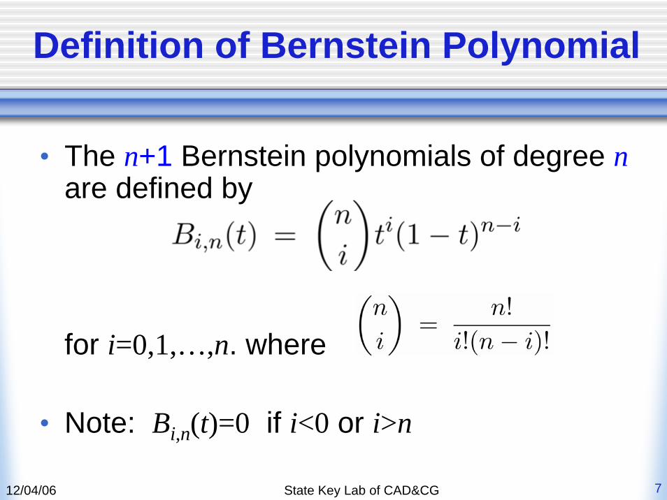
• The n+1 Bernstein polynomials of degree nare defined by
for i=0,1,…,n. where
• Note: Bi,n(t)=0 if i<0 or i>n
12/04/06 State Key Lab of CAD&CG 8
Example of Bernstein Polynomials (1)
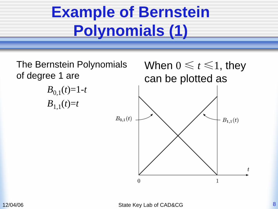
The Bernstein Polynomials of degree 1 are
B0,1(t)=1-tB1,1(t)=t
When 0 ≤ t ≤1, they can be plotted as
12/04/06 State Key Lab of CAD&CG 9
Example of Bernstein Polynomials (2)
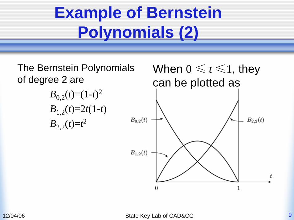
The Bernstein Polynomials of degree 2 are
B0,2(t)=(1-t)2
B1,2(t)=2t(1-t)B2,2(t)=t2
When 0 ≤ t ≤1, they can be plotted as
12/04/06 State Key Lab of CAD&CG 10
Example of Bernstein Polynomials (3)
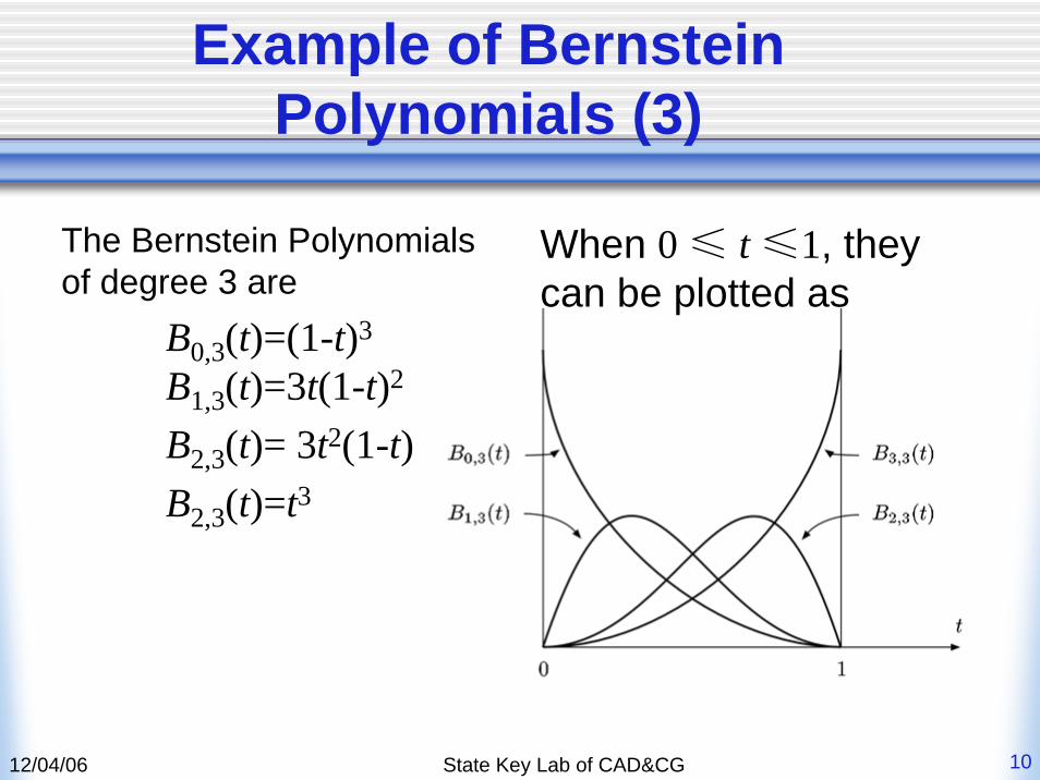
The Bernstein Polynomials of degree 3 are
B0,3(t)=(1-t)3
B1,3(t)=3t(1-t)2
B2,3(t)= 3t2(1-t)B2,3(t)=t3
When 0 ≤ t ≤1, they can be plotted as
12/04/06 State Key Lab of CAD&CG 11
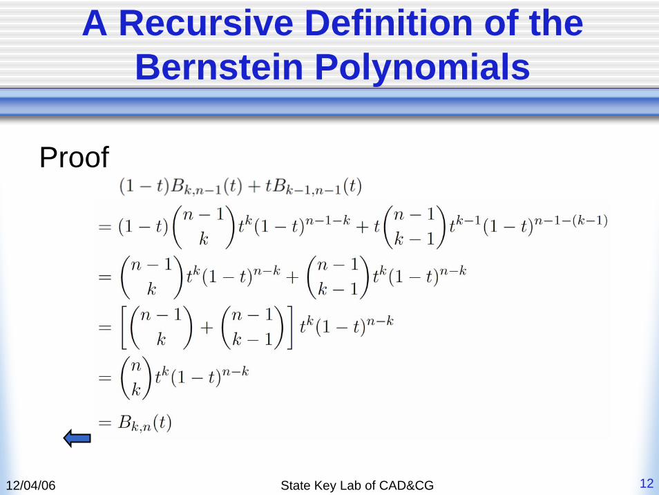
A Recursive Definition of the Bernstein Polynomials
• The Bernstein polynomials of degree ncan be defined by blending together twoBernstein polynomials of degree n-1
Bk,n(t)=(1-t) Bk,n-1(t)+tBk-1,n-1(t)The above statement can be proved by utilizing definition of the Bernstein polynomials
12/04/06 State Key Lab of CAD&CG 12
A Recursive Definition of the Bernstein Polynomials
Proof
12/04/06 State Key Lab of CAD&CG 13
Properties of Bernstein Polynomial
• Non-Negative• Partition of Unity • Symmetry• Degree Raising • Linear Precision• Derivatives
12/04/06 State Key Lab of CAD&CG 14
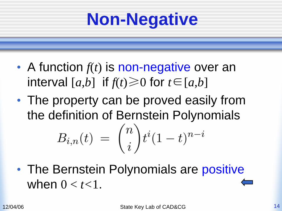
Non-Negative
• A function f(t) is non-negative over an interval [a,b] if f(t)≥0 for t∈[a,b]
• The property can be proved easily from the definition of Bernstein Polynomials
• The Bernstein Polynomials are positivewhen 0 < t<1.
12/04/06 State Key Lab of CAD&CG 15
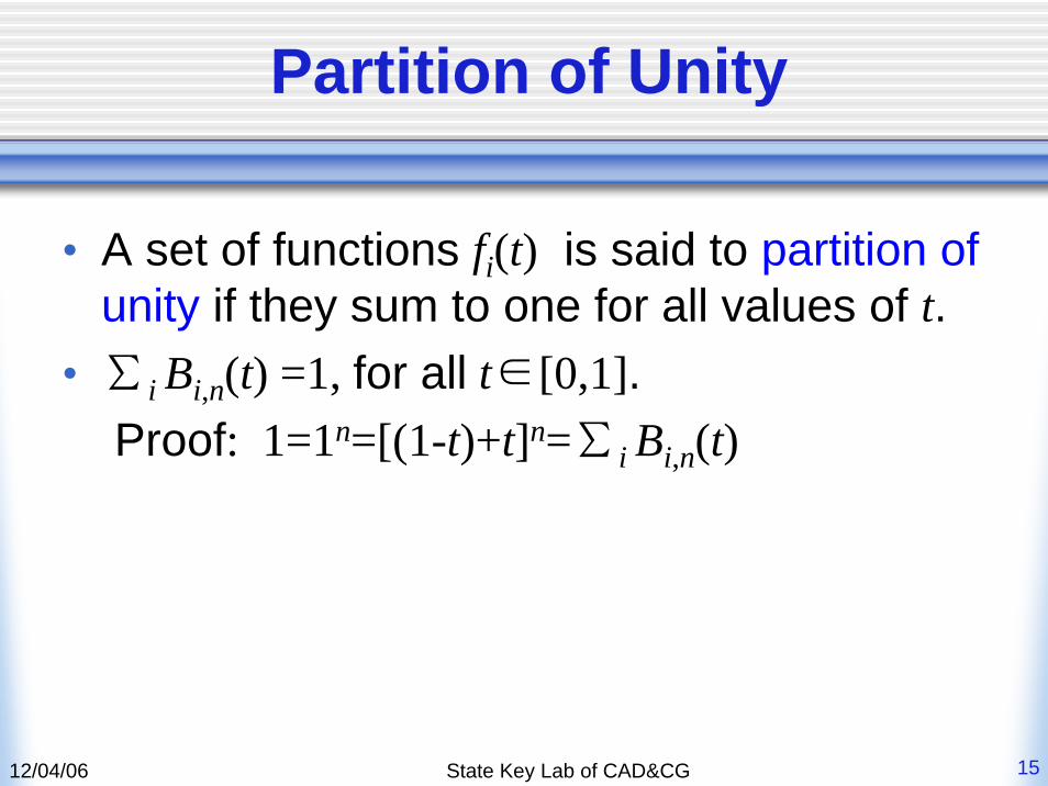
Partition of Unity
• A set of functions fi(t) is said to partition of unity if they sum to one for all values of t.
• ∑i Bi,n(t) =1, for all t∈[0,1].Proof: 1=1n=[(1-t)+t]n=∑i Bi,n(t)
12/04/06 State Key Lab of CAD&CG 16
Partition of Unity
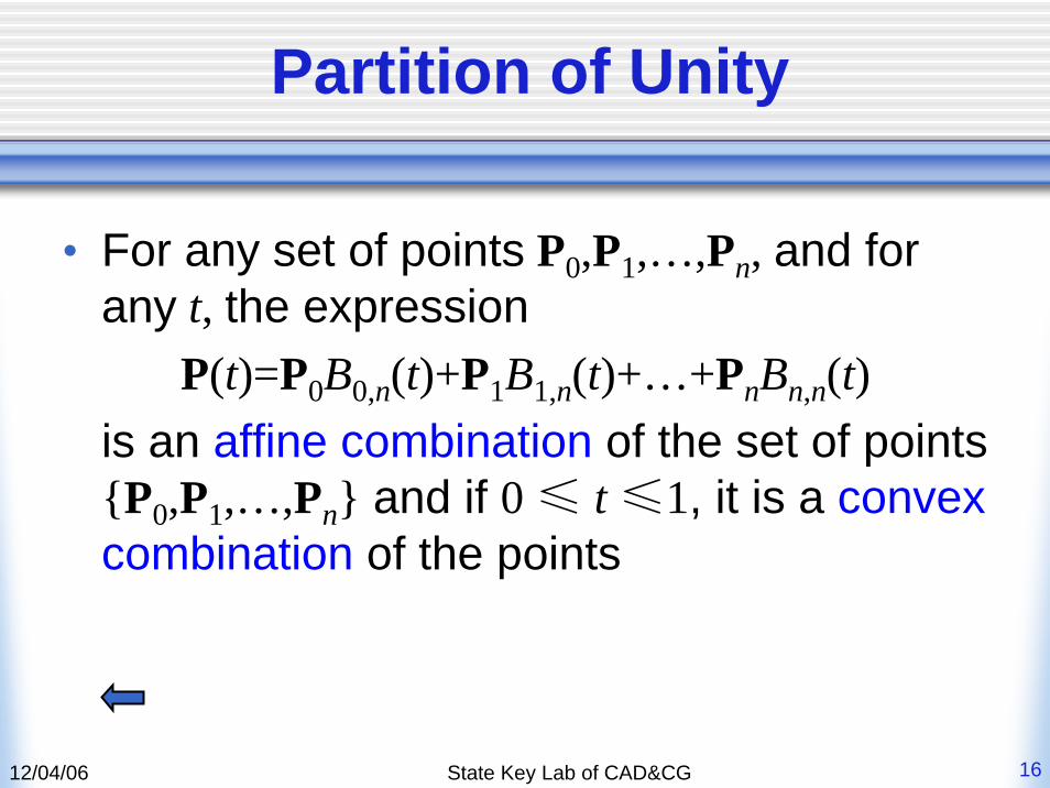
• For any set of points P0,P1,…,Pn, and for any t, the expression
P(t)=P0B0,n(t)+P1B1,n(t)+…+PnBn,n(t) is an affine combination of the set of points {P0,P1,…,Pn} and if 0 ≤ t ≤1, it is a convex combination of the points
12/04/06 State Key Lab of CAD&CG 17
Symmetry
• Bi,n(t)= Bn-i,n(1-t) • Proof: from definition……

12/04/06 State Key Lab of CAD&CG 18
Degree Raising
• Any of the lower-degree Bernstein polynomials (degree < n) can be expressed as a linear combination of Bernstein polynomials of degree n.
• Any Bernstein polynomial of degree n-1can be written as a linear combination of Bernstein polynomials of degree n.
( ) ( ) ( ), , 1 1, 11 1
1 1i n i n i nn i iB t B t B t
n n+ + +
− + += +
+ +
12/04/06 State Key Lab of CAD&CG 19
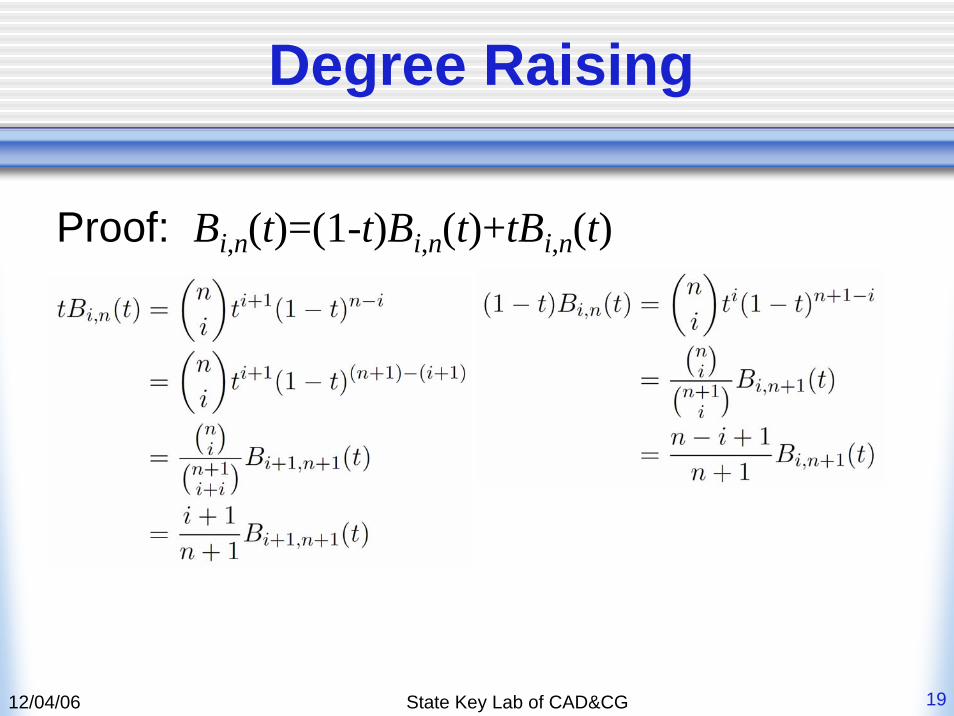
Degree Raising
Proof: Bi,n(t)=(1-t)Bi,n(t)+tBi,n(t)
12/04/06 State Key Lab of CAD&CG 20
Degree Raising
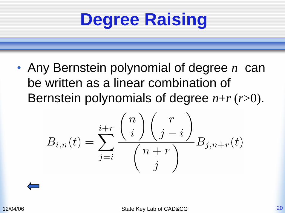
• Any Bernstein polynomial of degree n can be written as a linear combination of Bernstein polynomials of degree n+r (r>0).
12/04/06 State Key Lab of CAD&CG 21
Linear Precision
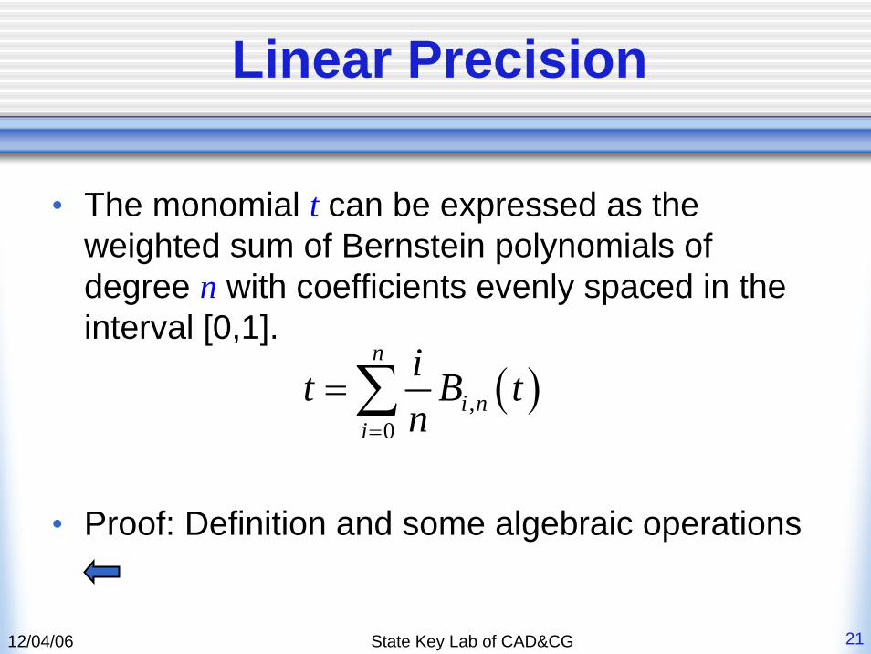
• The monomial t can be expressed as the weighted sum of Bernstein polynomials of degree n with coefficients evenly spaced in the interval [0,1].
• Proof: Definition and some algebraic operations
( ),0
n
i ni
it B tn=
= ∑
12/04/06 State Key Lab of CAD&CG 22
Derivatives
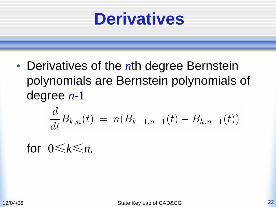
• Derivatives of the nth degree Bernstein polynomials are Bernstein polynomials of degree n-1
for 0≤k≤n.
12/04/06 State Key Lab of CAD&CG 23
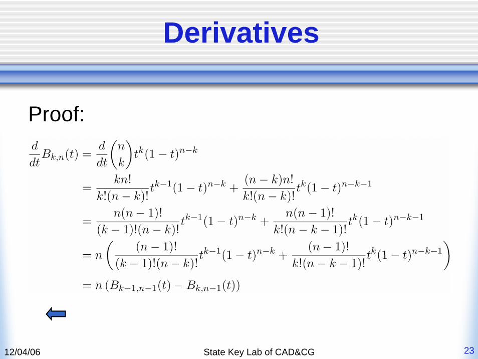
Derivatives
Proof:
12/04/06 State Key Lab of CAD&CG 24
Conversion Between Bernstein Basis and Power Basis
• Conversion from the Bernstein Basis to the Power Basis
• Conversion from the Power Basis to the Bernstein Basis
• The Bernstein Polynomials as a Basis of Polynomial Space
12/04/06 State Key Lab of CAD&CG 25
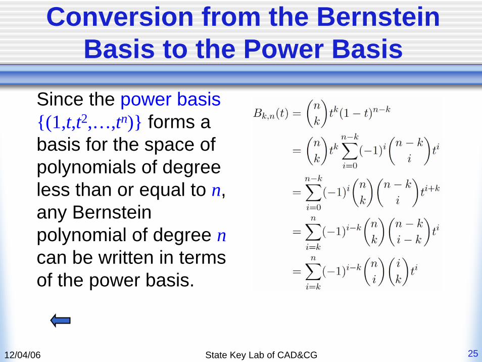
Conversion from the Bernstein Basis to the Power Basis
Since the power basis {(1,t,t2,…,tn)} forms a basis for the space of polynomials of degree less than or equal to n, any Bernstein polynomial of degree ncan be written in terms of the power basis.
12/04/06 State Key Lab of CAD&CG 26
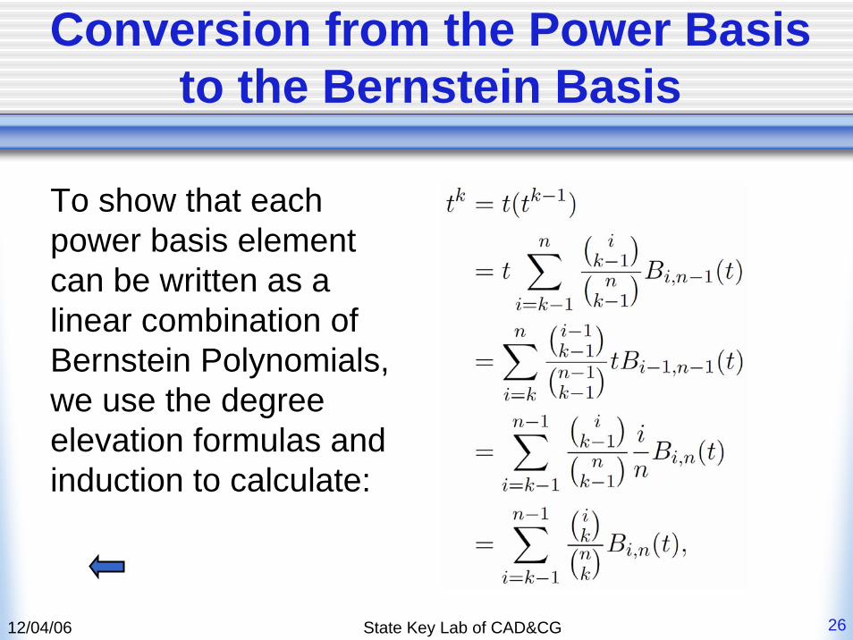
Conversion from the Power Basis to the Bernstein Basis
To show that each power basis element can be written as a linear combination of Bernstein Polynomials, we use the degree elevation formulas and induction to calculate:
12/04/06 State Key Lab of CAD&CG 27
The Bernstein Polynomials as a Basis of Polynomial Space
• The Bernstein polynomials of degree nform a basis for the space of polynomials of degree less than or equal to n.
They span the space of polynomials of degree ≤ n: any polynomial of degree less than or equal to n can be written as a linear combination of the Bernstein polynomials They are linearly independent
12/04/06 State Key Lab of CAD&CG 28
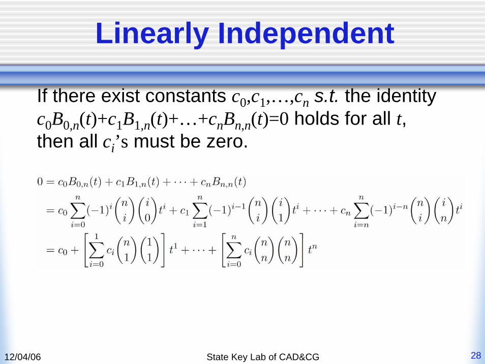
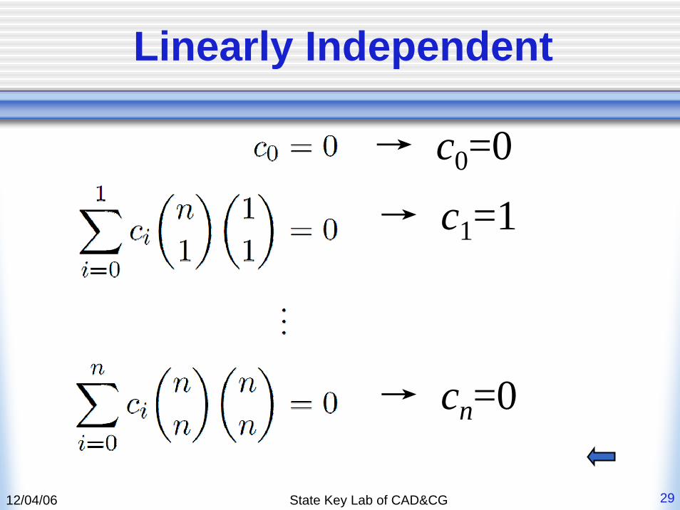
Linearly Independent
If there exist constants c0,c1,…,cn s.t. the identity c0B0,n(t)+c1B1,n(t)+…+cnBn,n(t)=0 holds for all t, then all ci’s must be zero.
12/04/06 State Key Lab of CAD&CG 29
Linearly Independent
→ c0=0
→ c1=1
→ cn=0
12/04/06 State Key Lab of CAD&CG 30
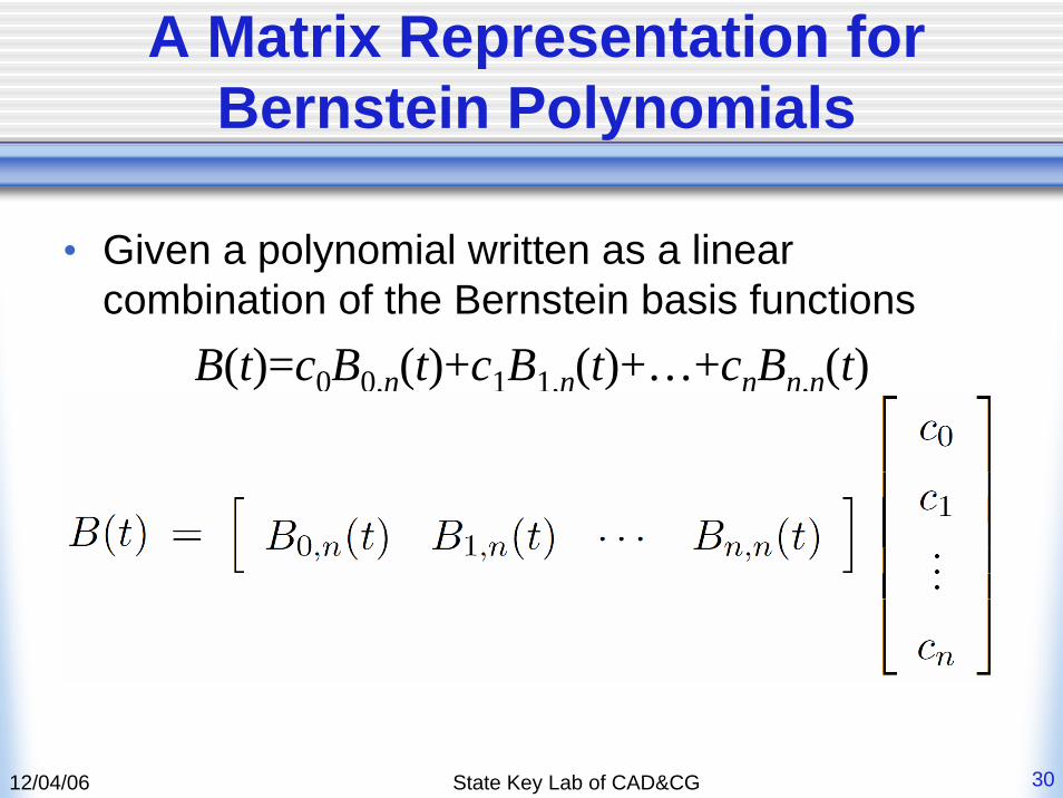
A Matrix Representation for Bernstein Polynomials
• Given a polynomial written as a linear combination of the Bernstein basis functions
B(t)=c0B0,n(t)+c1B1,n(t)+…+cnBn,n(t)
12/04/06 State Key Lab of CAD&CG 31
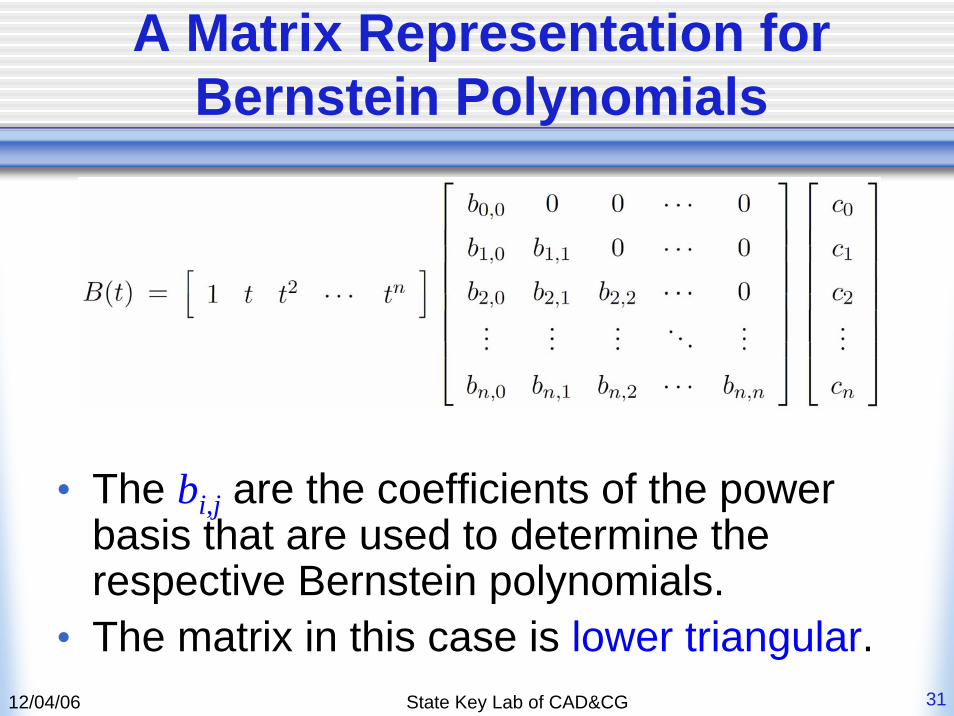
A Matrix Representation for Bernstein Polynomials
• The bi,j are the coefficients of the power basis that are used to determine the respective Bernstein polynomials.
• The matrix in this case is lower triangular.
12/04/06 State Key Lab of CAD&CG 32
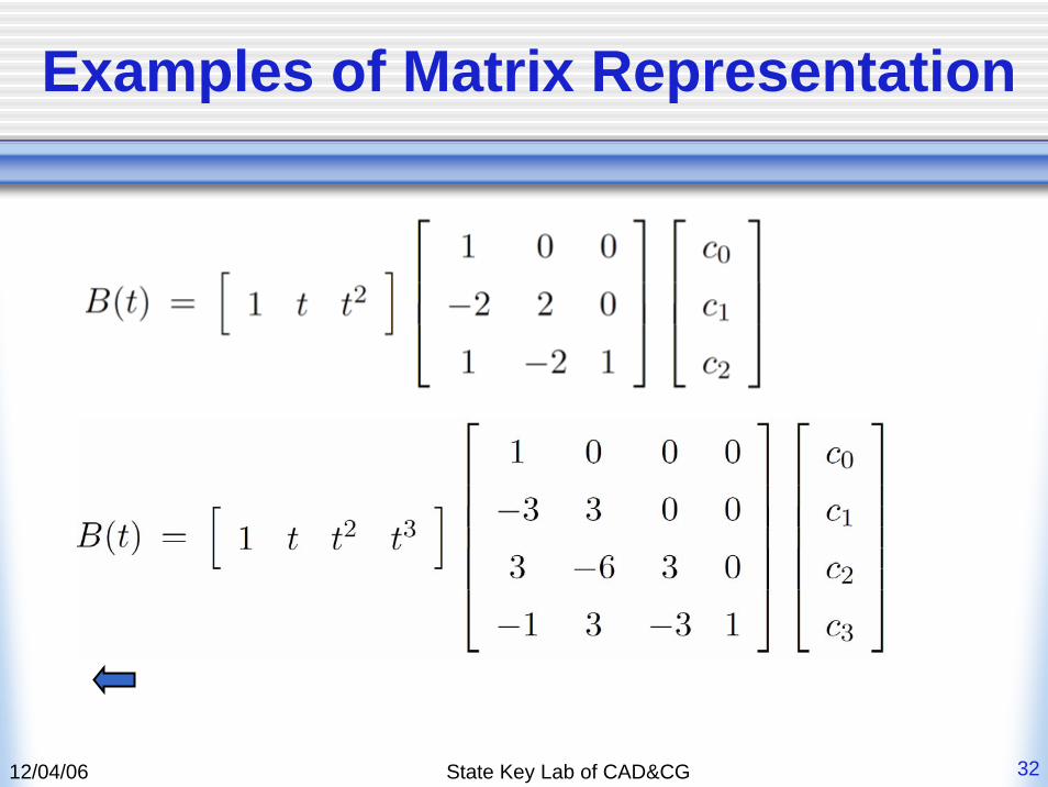
Examples of Matrix Representation
12/04/06 State Key Lab of CAD&CG 33
A Divide-and-Conquer Method for Drawing a Bézier Curve
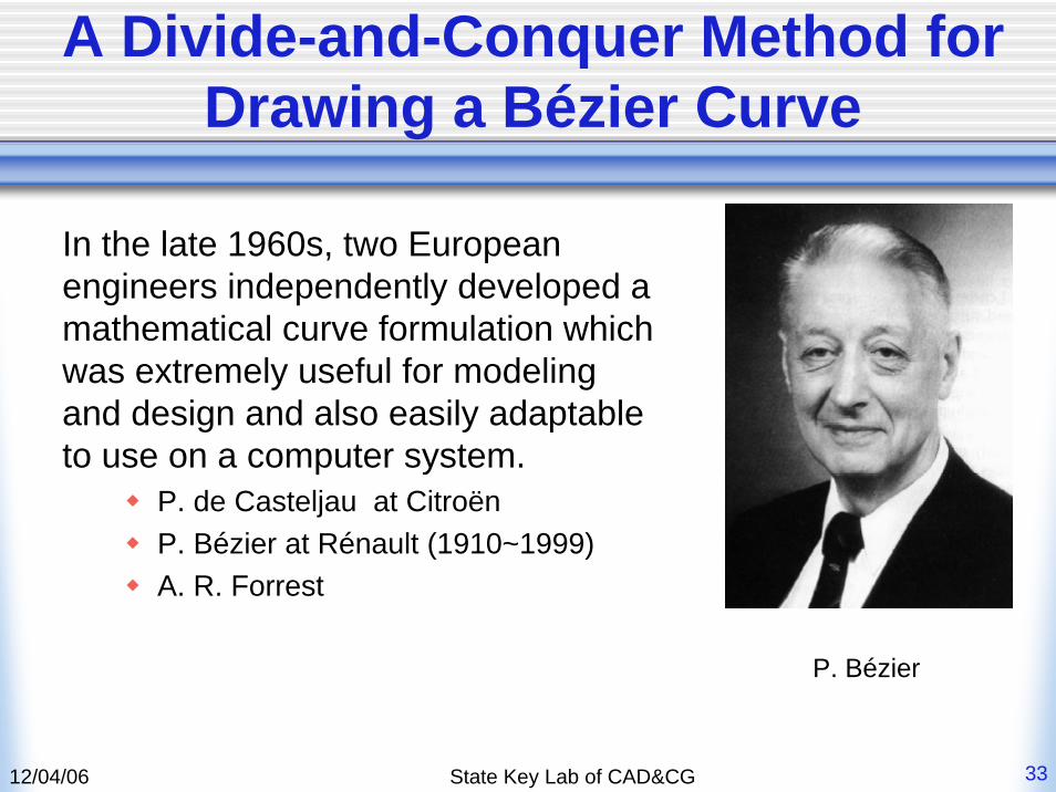
In the late 1960s, two European engineers independently developed a mathematical curve formulation which was extremely useful for modeling and design and also easily adaptable to use on a computer system.
P. de Casteljau at CitroënP. Bézier at Rénault (1910~1999)A. R. Forrest
P. Bézier
12/04/06 State Key Lab of CAD&CG 34
The Subdivision Procedure
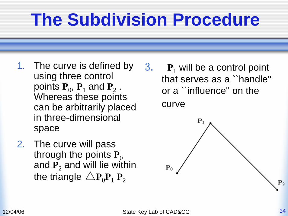
1. The curve is defined by using three control points P0, P1 and P2 . Whereas these points can be arbitrarily placed in three-dimensional space
2. The curve will pass through the points P0 and P2 and will lie within the triangle △P0P1 P2
3. P1 will be a control point that serves as a ``handle'' or a ``influence'' on the curve
12/04/06 State Key Lab of CAD&CG 35
The Subdivision Procedure
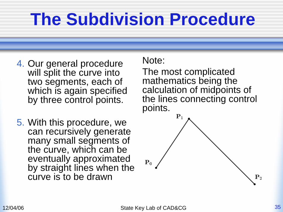
4. Our general procedure will split the curve into two segments, each of which is again specified by three control points.
5. With this procedure, we can recursively generate many small segments of the curve, which can be eventually approximated by straight lines when the curve is to be drawn
Note: The most complicated mathematics being the calculation of midpoints of the lines connecting control points.
12/04/06 State Key Lab of CAD&CG 36
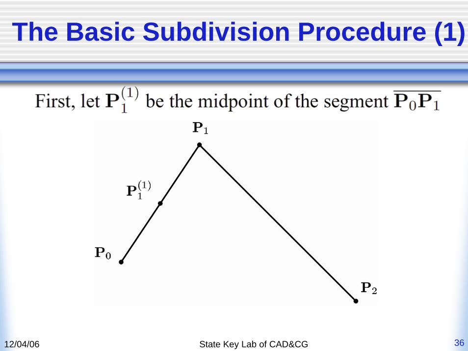
The Basic Subdivision Procedure (1)
12/04/06 State Key Lab of CAD&CG 37
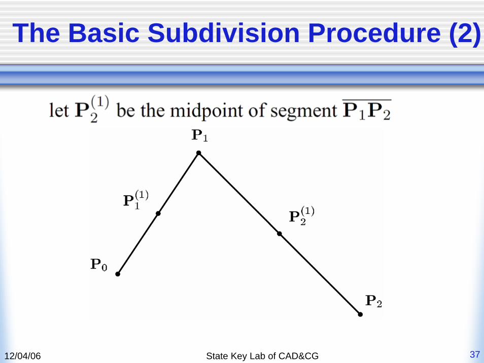
The Basic Subdivision Procedure (2)
12/04/06 State Key Lab of CAD&CG 38
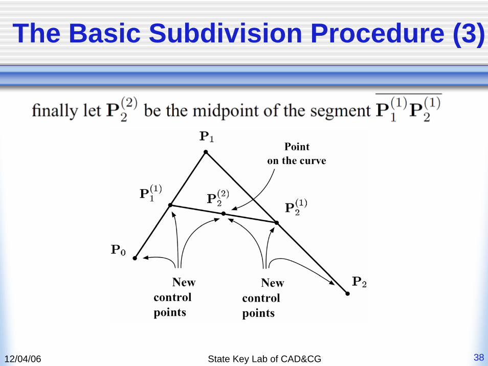
The Basic Subdivision Procedure (3)
12/04/06 State Key Lab of CAD&CG 39
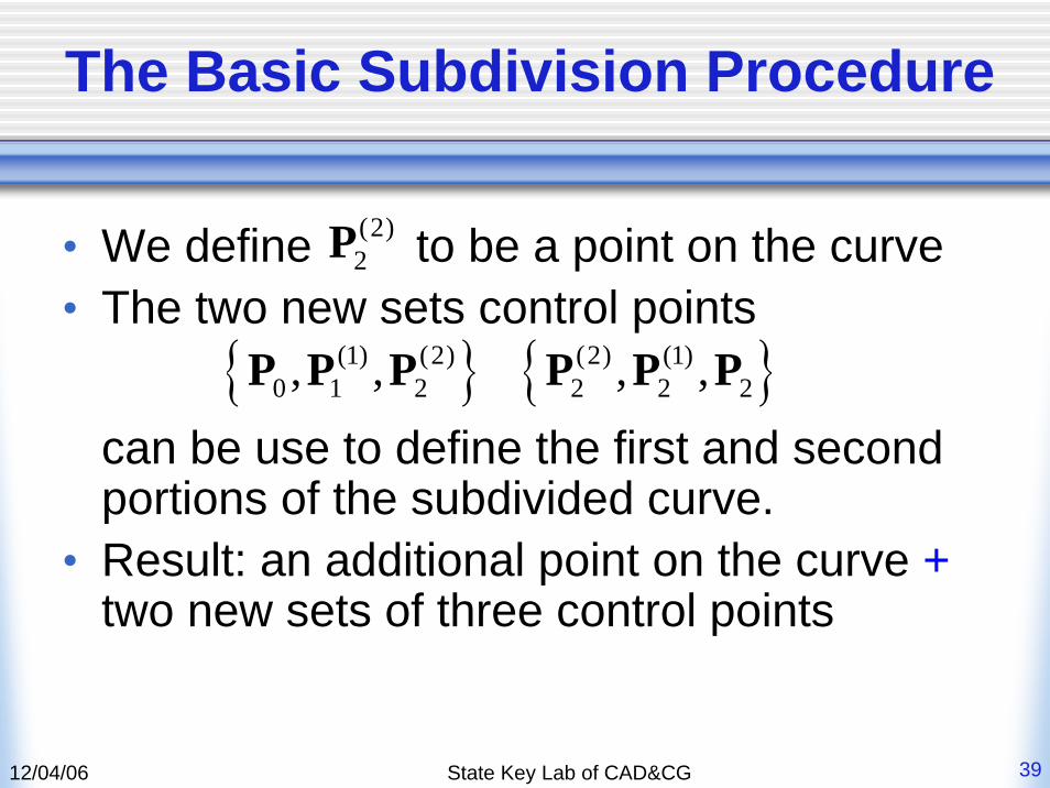
The Basic Subdivision Procedure
• We define to be a point on the curve• The two new sets control points
can be use to define the first and second portions of the subdivided curve.
• Result: an additional point on the curve +two new sets of three control points
(2)2P
{ }(1) (2)0 1 2, ,P P P { }(2) (1)
2 2 2, ,P P P
12/04/06 State Key Lab of CAD&CG 40
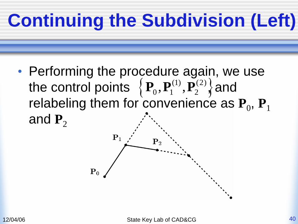
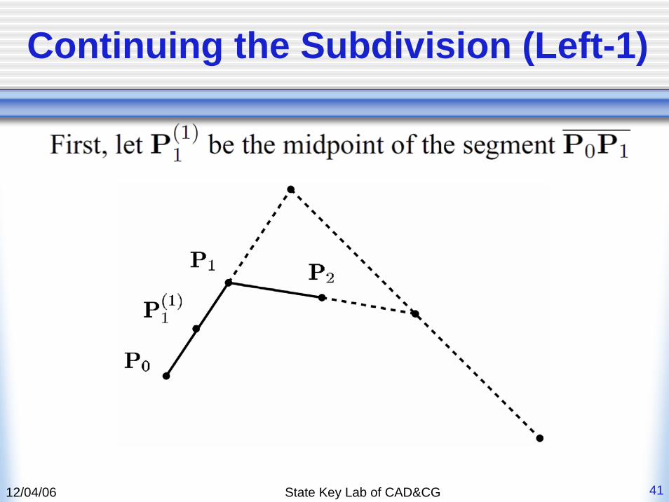
Continuing the Subdivision (Left)
• Performing the procedure again, we use the control points , and relabeling them for convenience as P0, P1and P2
{ }(1) (2)0 1 2, ,P P P
12/04/06 State Key Lab of CAD&CG 41
Continuing the Subdivision (Left-1)
12/04/06 State Key Lab of CAD&CG 42
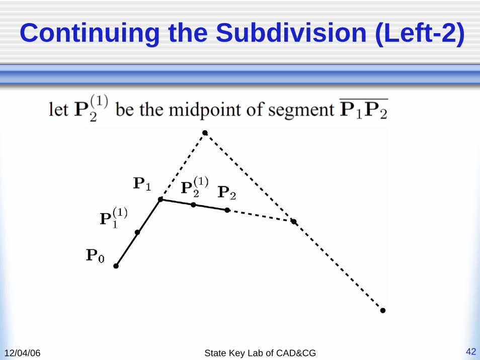
Continuing the Subdivision (Left-2)
12/04/06 State Key Lab of CAD&CG 43
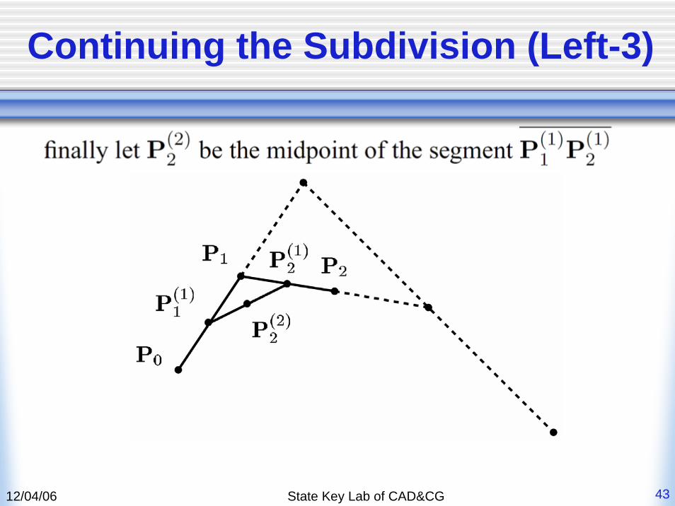
Continuing the Subdivision (Left-3)
12/04/06 State Key Lab of CAD&CG 44
Continuing the Subdivision (Left)
• We now define to be a point on the curve. This process produces another point on the curve, and creates two new sets of control points as was the case before.
(2)2P
12/04/06 State Key Lab of CAD&CG 45
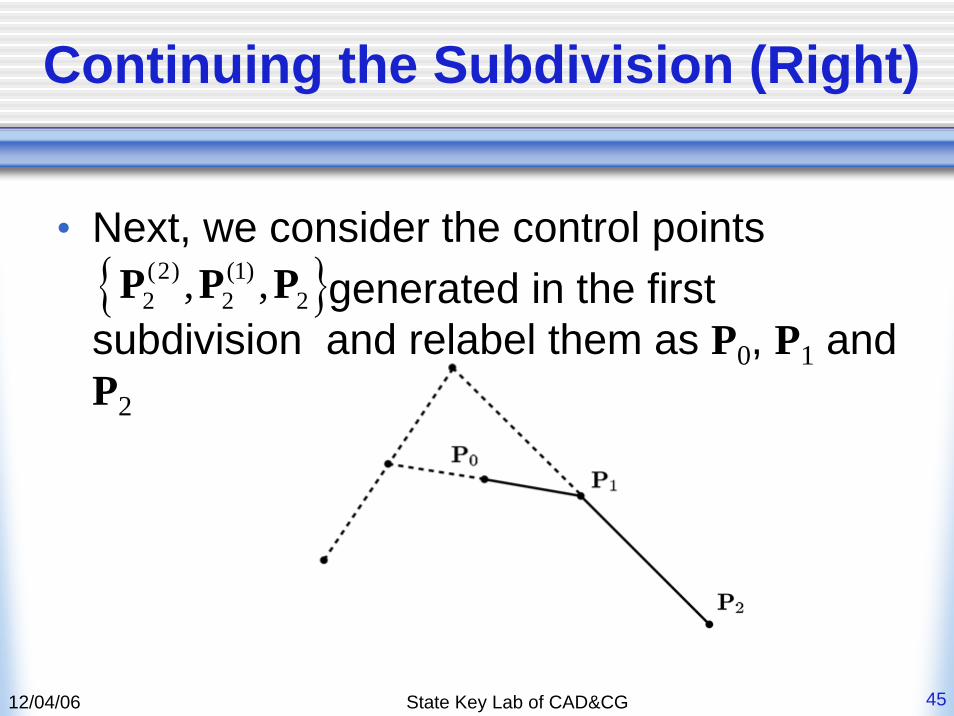
Continuing the Subdivision (Right)
• Next, we consider the control points generated in the first
subdivision and relabel them as P0, P1 and P2
{ }(2) (1)2 2 2, ,P P P
12/04/06 State Key Lab of CAD&CG 46
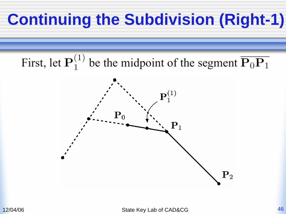
Continuing the Subdivision (Right-1)

12/04/06 State Key Lab of CAD&CG 47
Continuing the Subdivision (Right-2)
12/04/06 State Key Lab of CAD&CG 48
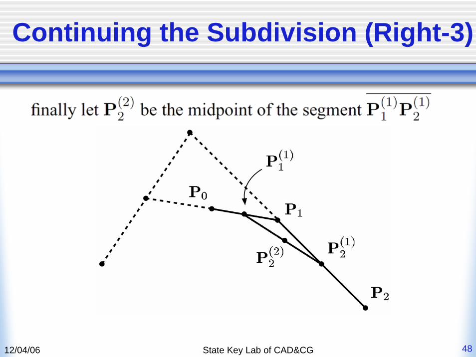
Continuing the Subdivision (Right-3)

12/04/06 State Key Lab of CAD&CG 49
Continuing the Subdivision (Right)
• We now have on the curve . (2)2P
12/04/06 State Key Lab of CAD&CG 50
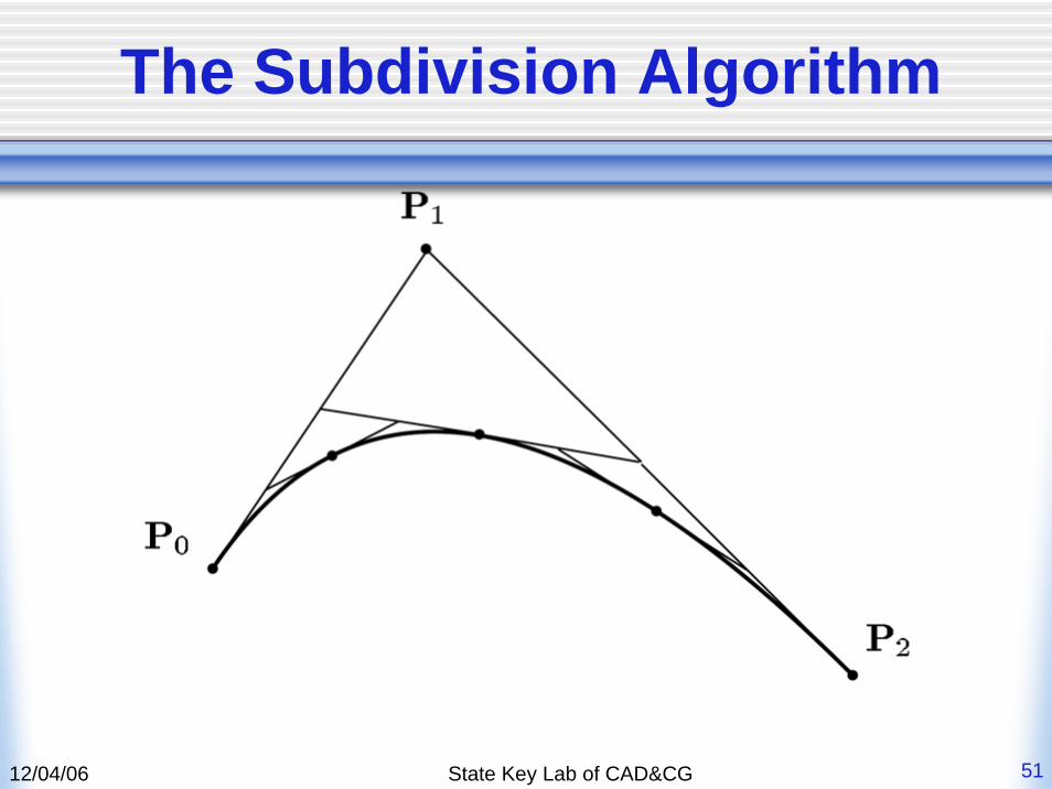
The Subdivision Algorithm
• Three points have now been generated on the curve and four subcurves have been generated.
• At each step the process creates both a point on the curve and two new sets of control points.
• This effectively subdivides the curve into two new curve segments, each of which can be handled separately.
12/04/06 State Key Lab of CAD&CG 51
The Subdivision Algorithm
12/04/06 State Key Lab of CAD&CG 52
Summary
• It is a geometric method, as it uses only the midpoint formula as it's fundamental tool.
• It uses the basic computer science paradigm of (sub)divide and conquer to calculate points on the curve.
• The curve can be ``drawn'' using computer graphics by calculating a somewhat-dense set of points, and connecting them with straight lines.
• The curve drawn by this method is a quadratic Bézier curve.
12/04/06 State Key Lab of CAD&CG 53
Quadratic Bezier Curves
• Development of the Quadratic Bézier Curve
• Developing the Equation of the Curve • Properties of the Quadratic Curve • Summarizing the Development of the
Curve
12/04/06 State Key Lab of CAD&CG 54
Development of the Quadratic Bézier Curve
• Given three control points P0, P1 and P2 ,we develop a divide procedure that is based upon a parameter t , which is a number between 0 and 1 ( the illustrations utilize the value 0.75 ).
12/04/06 State Key Lab of CAD&CG 55
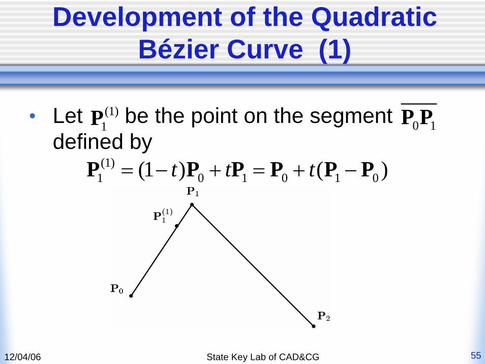
Development of the Quadratic Bézier Curve (1)
• Let be the point on the segment defined by
(1)1P 0 1P P
(1)1 0 1 0 1 0(1 ) ( )t t t= − + = + −P P P P P P
12/04/06 State Key Lab of CAD&CG 56
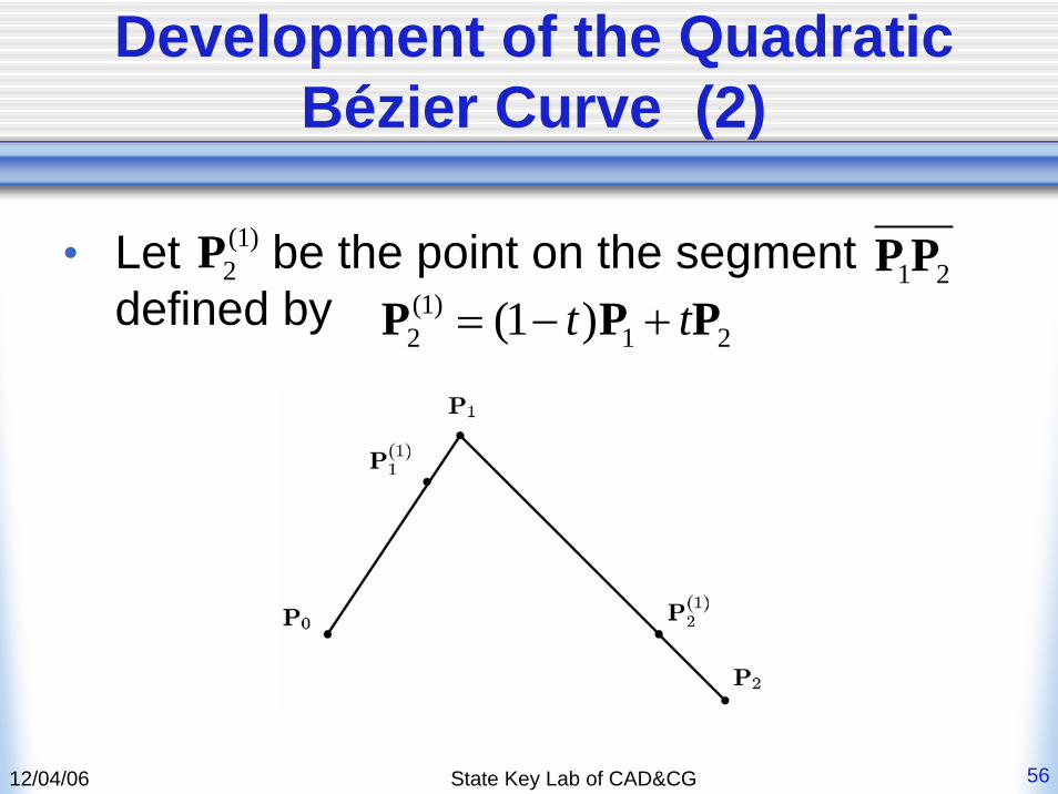
Development of the Quadratic Bézier Curve (2)
• Let be the point on the segment defined by
(1)2P 1 2P P
(1)2 1 2(1 )t t= − +P P P
12/04/06 State Key Lab of CAD&CG 57
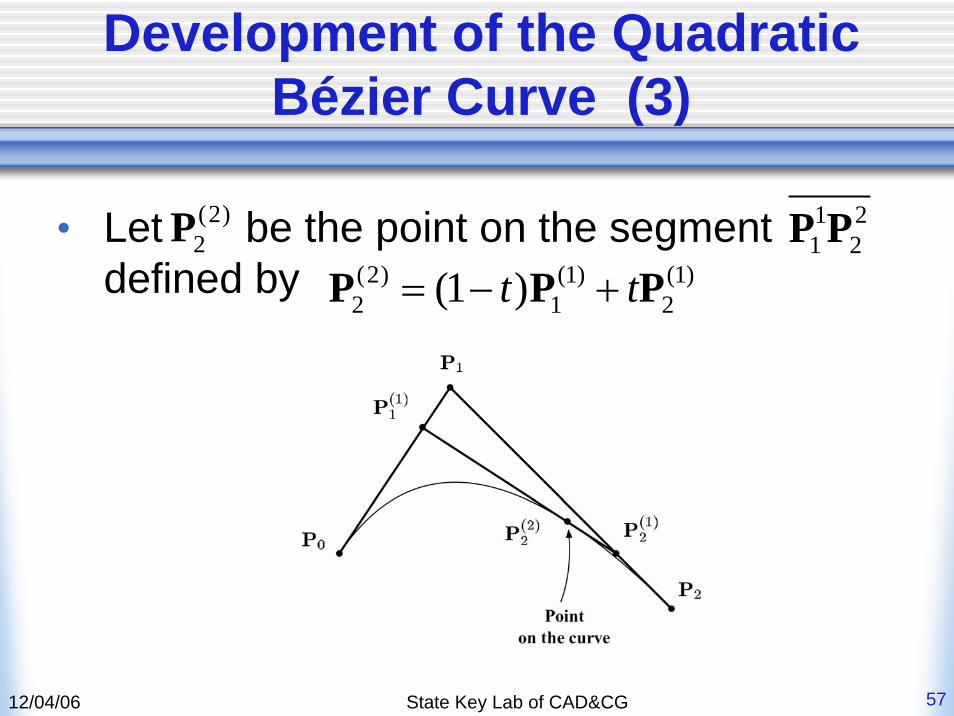
Development of the Quadratic Bézier Curve (3)
• Let be the point on the segment defined by
(2)2P 1 2
1 2P P(2) (1) (1)2 1 2(1 )t t= − +P P P
12/04/06 State Key Lab of CAD&CG 58
Development of the Quadratic Bézier Curve (4)
• Define
• Note1. It is a geometric mean to define points on
the curve.2. It is identical to the divide-and-conquer
method in the case t=1/2.
(2)2( )t =P P
12/04/06 State Key Lab of CAD&CG 59
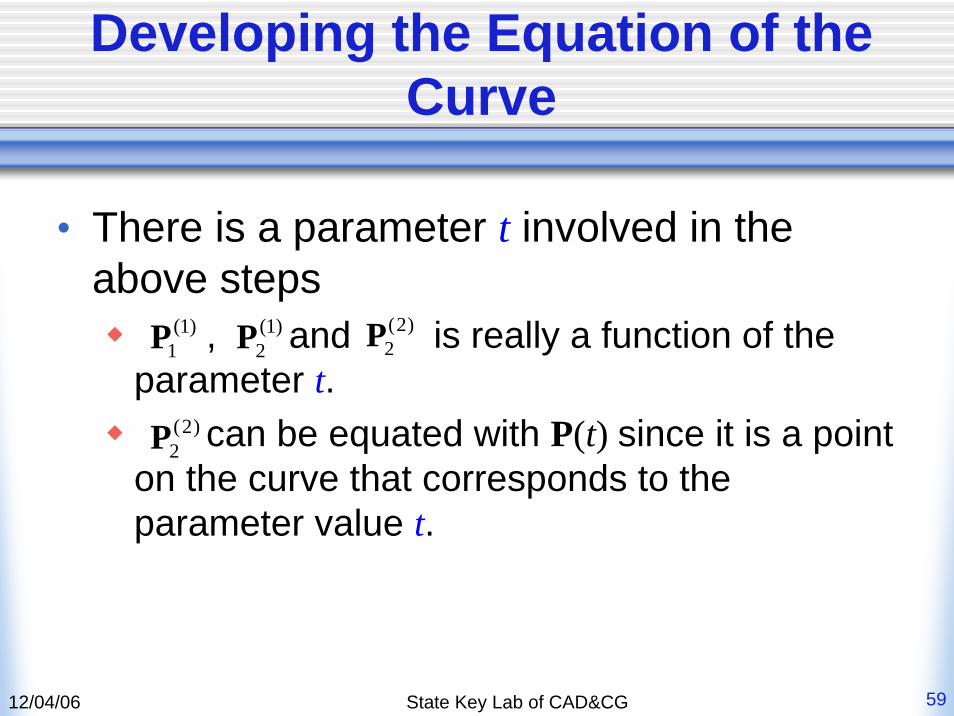
Developing the Equation of the Curve
• There is a parameter t involved in the above steps
, and is really a function of the parameter t.
can be equated with P(t) since it is a point on the curve that corresponds to the parameter value t.
(1)1P (1)
2P (2)2P
(2)2P
12/04/06 State Key Lab of CAD&CG 60
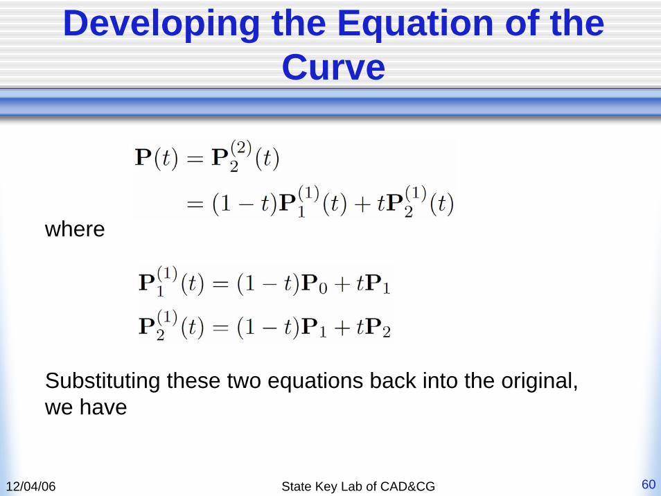
Developing the Equation of the Curve
where
Substituting these two equations back into the original, we have
12/04/06 State Key Lab of CAD&CG 61
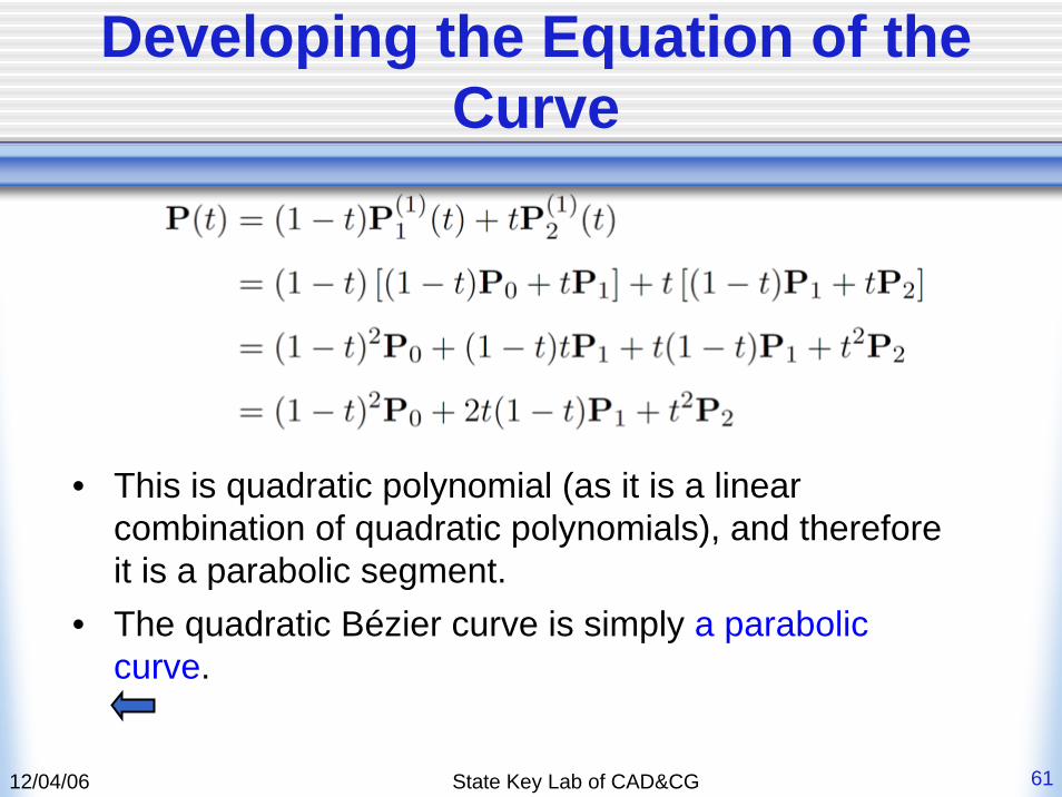
Developing the Equation of the Curve
• This is quadratic polynomial (as it is a linear combination of quadratic polynomials), and therefore it is a parabolic segment.
• The quadratic Bézier curve is simply a parabolic curve.
12/04/06 State Key Lab of CAD&CG 62
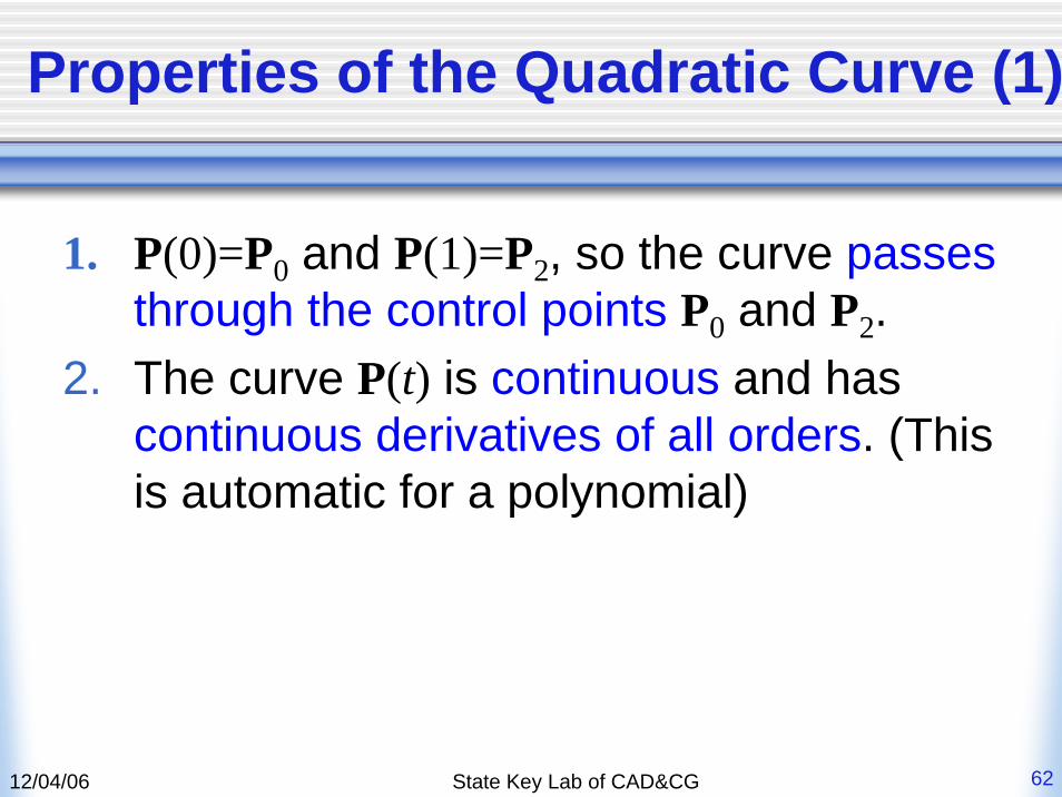
Properties of the Quadratic Curve (1)
1. P(0)=P0 and P(1)=P2, so the curve passes through the control points P0 and P2.
2. The curve P(t) is continuous and has continuous derivatives of all orders. (This is automatic for a polynomial)
12/04/06 State Key Lab of CAD&CG 63
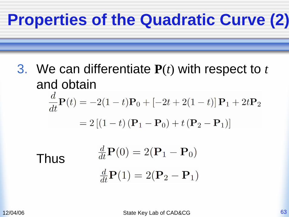
Properties of the Quadratic Curve (2)
3. We can differentiate P(t) with respect to tand obtain
Thus
12/04/06 State Key Lab of CAD&CG 64
Properties of the Quadratic Curve (3)
4. The functions (1-t)2, 2t(1-t) and t2 that are used to “blend” the control points P0, P1 and P2 together are the degree-2 Bernstein Polynomials. They are all non-negative functions and sum to one.
5. The curve is contained within the triangle △P0P1P2. Since
P(t) is a convex combination of the points P0, P1 and P2. The convex hull of a triangle is the triangle itself.
12/04/06 State Key Lab of CAD&CG 65
Properties of the Quadratic Curve (4)
6. If the points P0, P1 and P2 are colinear, then the curve is a straight line.
7. The process of calculating one P(t)subdivides the control points into two sets and , each of which can be used to define another curve, as in our subdivision process above.
{ }(1) (2)0 1 2, ,P P P { }(2) (1)
2 2 2, ,P P P
12/04/06 State Key Lab of CAD&CG 66
Properties of the Quadratic Curve (4)
8. All the points, generated from the divide-and-conquer method, lie on this curve.
12/04/06 State Key Lab of CAD&CG 67
Summarizing the Development of the Curve
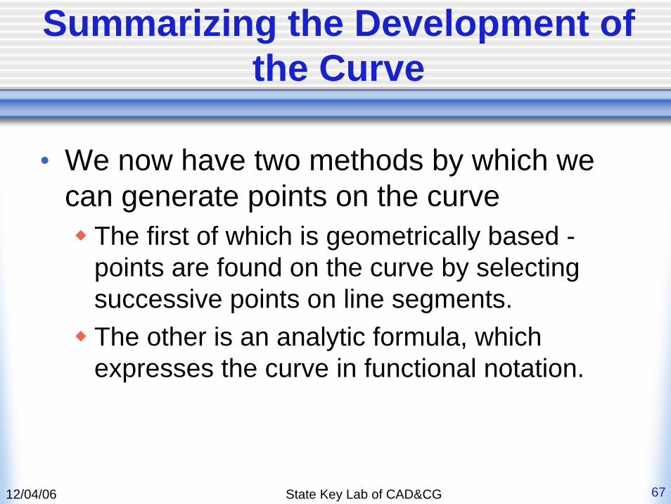
• We now have two methods by which we can generate points on the curve
The first of which is geometrically based -points are found on the curve by selecting successive points on line segments. The other is an analytic formula, which expresses the curve in functional notation.
12/04/06 State Key Lab of CAD&CG 68
The Geometrical Construction Method
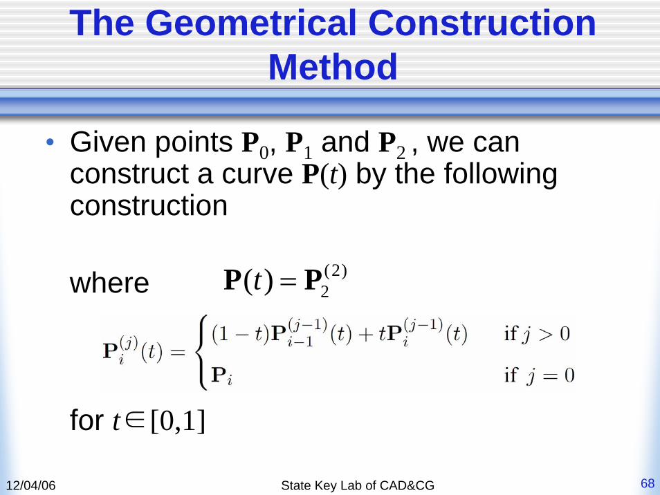
• Given points P0, P1 and P2 , we can construct a curve P(t) by the following construction
where
for t∈[0,1]
(2)2( )t =P P
12/04/06 State Key Lab of CAD&CG 69
The Analytical Formula
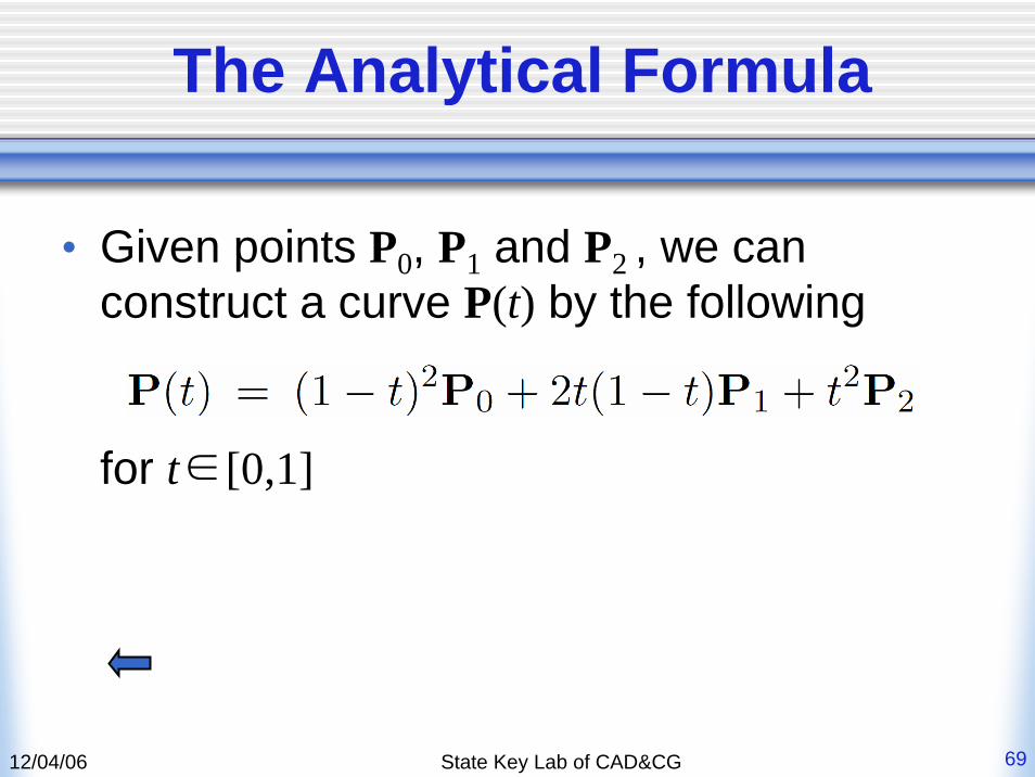
• Given points P0, P1 and P2 , we can construct a curve P(t) by the following
for t∈[0,1]
12/04/06 State Key Lab of CAD&CG 70
Cubic Bézier Curve – Geometric Construction
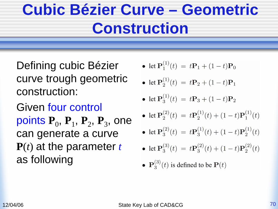
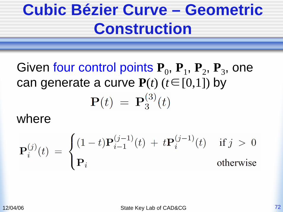
Defining cubic Bézier curve trough geometric construction:Given four control points P0, P1, P2, P3, one can generate a curve P(t) at the parameter tas following
12/04/06 State Key Lab of CAD&CG 71
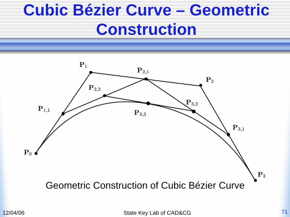
Cubic Bézier Curve – Geometric Construction
Geometric Construction of Cubic Bézier Curve
12/04/06 State Key Lab of CAD&CG 72
Cubic Bézier Curve – Geometric Construction
Given four control points P0, P1, P2, P3, one can generate a curve P(t) (t∈[0,1]) by
where
12/04/06 State Key Lab of CAD&CG 73
Cubic Bézier Curve –Analytical Construction
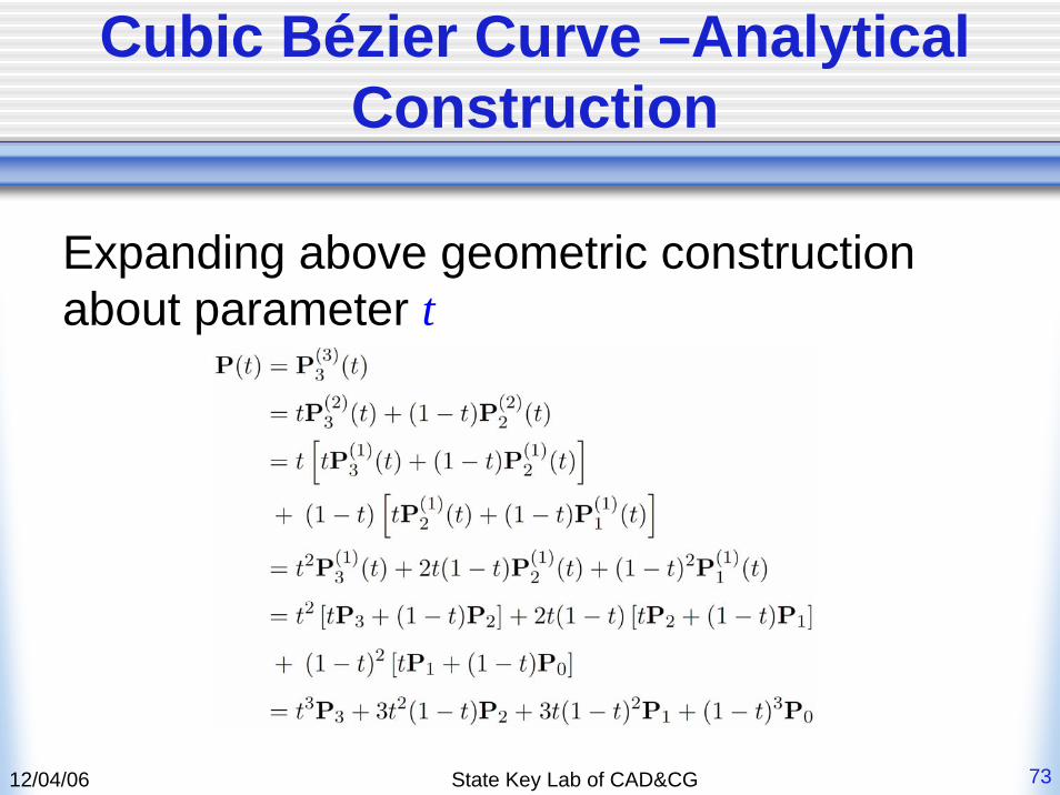
Expanding above geometric construction about parameter t
12/04/06 State Key Lab of CAD&CG 74
Cubic Bézier Curve –Analytical Construction
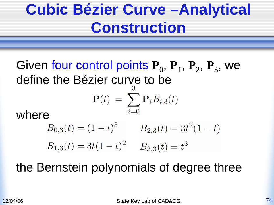
Given four control points P0, P1, P2, P3, we define the Bézier curve to be
where
the Bernstein polynomials of degree three
12/04/06 State Key Lab of CAD&CG 75
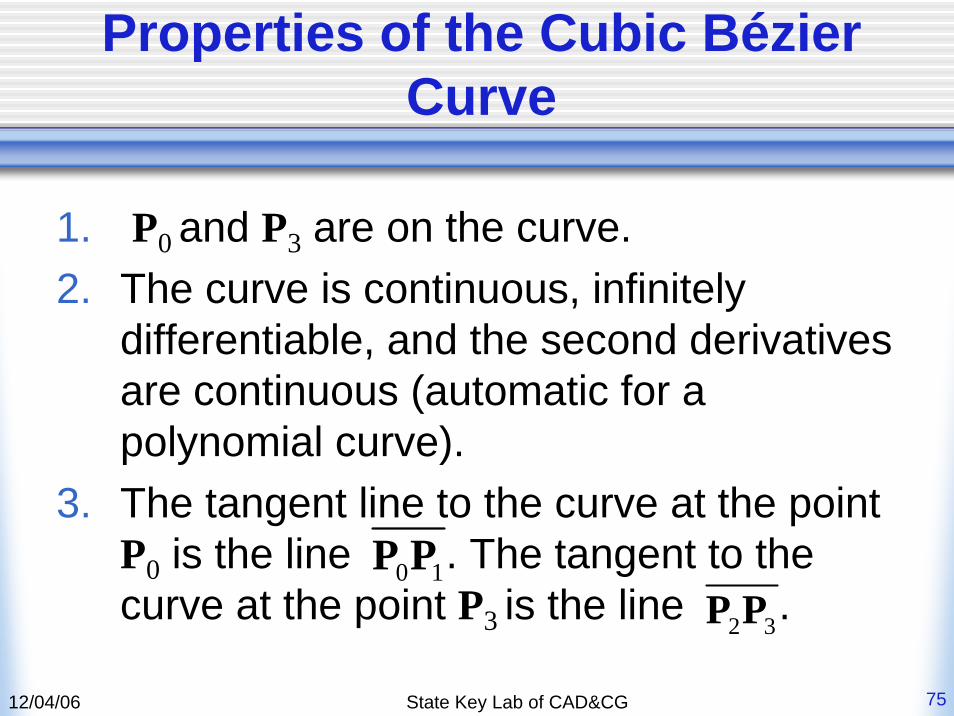
Properties of the Cubic Bézier Curve
1. P0 and P3 are on the curve. 2. The curve is continuous, infinitely
differentiable, and the second derivatives are continuous (automatic for a polynomial curve).
3. The tangent line to the curve at the point P0 is the line . The tangent to the curve at the point P3 is the line . 2 3P P
0 1P P
12/04/06 State Key Lab of CAD&CG 76
Properties of the Cubic Bézier Curve
• The curve lies within the convex hull of its control points.
• Both P1 and P2 are on the curve only if the curve is linear.
12/04/06 State Key Lab of CAD&CG 77
A Matrix Representation for Cubic Bezier Curves
• Overview• Developing the Matrix Equation • Subdivision Using the Matrix Form • Generating a Sequence of Bézier Control
Polygons
12/04/06 State Key Lab of CAD&CG 78
Overview
• Purposes of matrix representationFast computation of matrices multiplicationGenerating different Bézier control polygons for the cubic curve
12/04/06 State Key Lab of CAD&CG 79
Developing the Matrix Equation
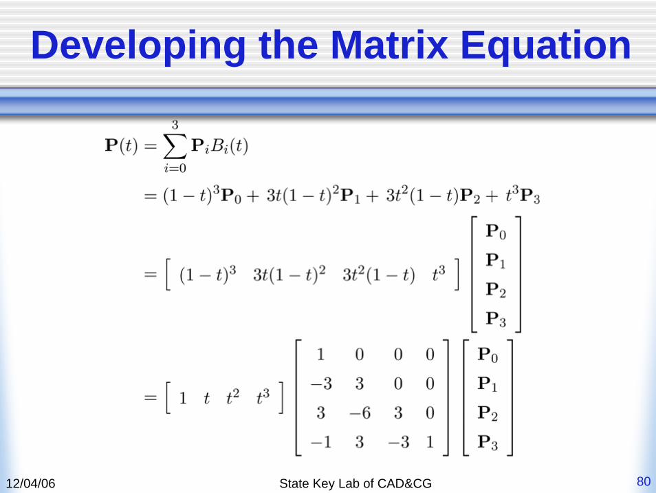
• A cubic Bézier Curve can be written in a matrix form
1. Expanding the analytic definition of the curve into its Bernstein polynomial coefficients,
2. Then writing these coefficients in a matrix form using the polynomial power basis.
12/04/06 State Key Lab of CAD&CG 80
Developing the Matrix Equation
12/04/06 State Key Lab of CAD&CG 81
Developing the Matrix Equation
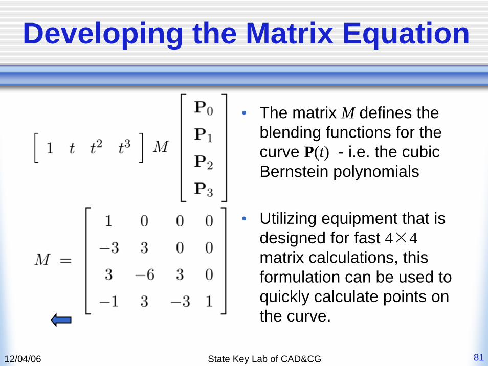
• The matrix M defines the blending functions for the curve P(t) - i.e. the cubic Bernstein polynomials
• Utilizing equipment that is designed for fast 4×4matrix calculations, this formulation can be used to quickly calculate points on the curve.
12/04/06 State Key Lab of CAD&CG 82
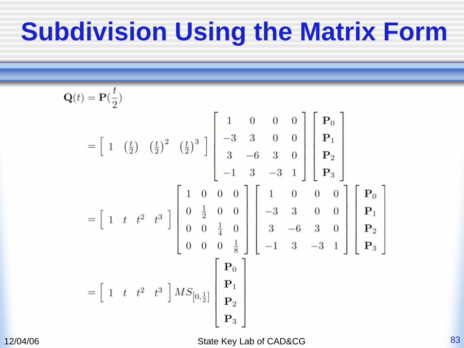
Subdivision Using the Matrix Form
• Suppose we wish to generate the control polygon for the portion of the curve P(t)where t ranges between 0 and 1/2
Clearly this new curve is a cubic polynomial, and traces the desired portion of P as t ranges between 0 and 1For the control points of the new curve Q(t)
Geometric ConstructionUsing matrix form of the curve P
12/04/06 State Key Lab of CAD&CG 83
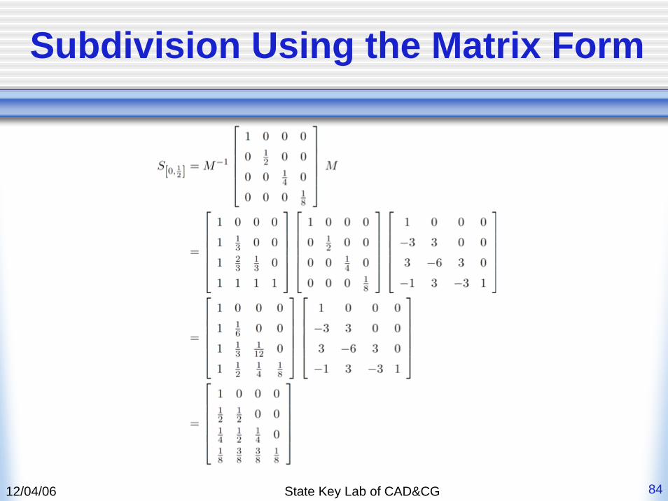
Subdivision Using the Matrix Form
12/04/06 State Key Lab of CAD&CG 84
Subdivision Using the Matrix Form
12/04/06 State Key Lab of CAD&CG 85
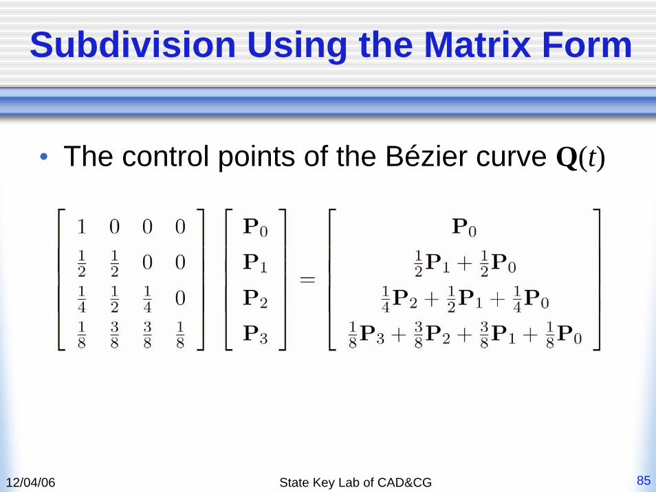
Subdivision Using the Matrix Form
• The control points of the Bézier curve Q(t)
12/04/06 State Key Lab of CAD&CG 86
Subdivision Using the Matrix Form
• Similarly, the Bézier control polygon for the second half of the curve t∈[1/2,1] can be obtained as following
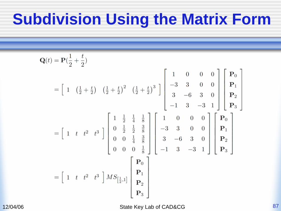
12/04/06 State Key Lab of CAD&CG 87
Subdivision Using the Matrix Form
12/04/06 State Key Lab of CAD&CG 88
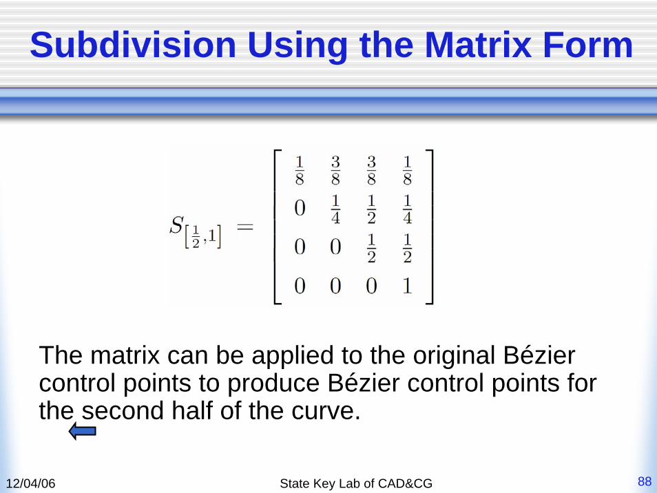
Subdivision Using the Matrix Form
The matrix can be applied to the original Bézier control points to produce Bézier control points for the second half of the curve.
12/04/06 State Key Lab of CAD&CG 89
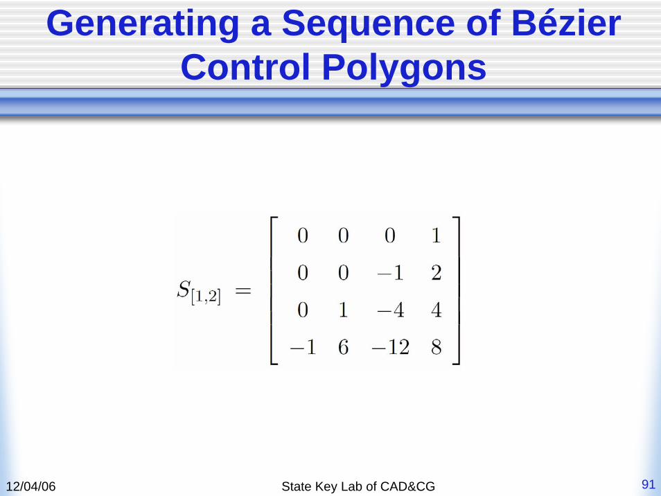
Generating a Sequence of Bézier Control Polygons
• Using matrix calculations similar to those above, we can generate an iterative scheme to generate a sequence of points on the curve
• If we consider the portion of the cubic curve where P(t) ranges between 1 and 2 , we generate the Bézier control points of Q(t) by reparameterization of the original curve - namely by replacing t by t+1

12/04/06 State Key Lab of CAD&CG 90
Generating a Sequence of Bézier Control Polygons
12/04/06 State Key Lab of CAD&CG 91
Generating a Sequence of Bézier Control Polygons
12/04/06 State Key Lab of CAD&CG 92
Generating a Sequence of Bézier Control Polygons
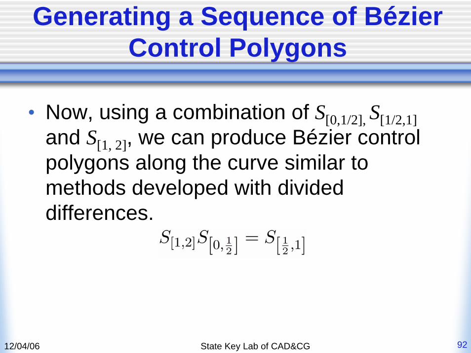
• Now, using a combination of S[0,1/2], S[1/2,1]and S[1, 2], we can produce Bézier control polygons along the curve similar to methods developed with divided differences.

12/04/06 State Key Lab of CAD&CG 93
Generating a Sequence of Bézier Control Polygons
Applying S[0,1/2] to obtain a Bézier control polygon for the first half of the curveApplying S[1, 2] to this control polygon to obtain the Bézier control polygon for the second half of the curve
12/04/06 State Key Lab of CAD&CG 94
Generating a Sequence of Bézier Control Polygons
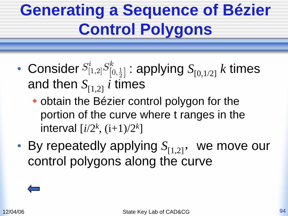
• Consider : applying S[0,1/2] k times and then S[1,2] i times
obtain the Bézier control polygon for the portion of the curve where t ranges in the interval [i/2k, (i+1)/2k]
• By repeatedly applying S[1,2],we move our control polygons along the curve