c© 2007 Abhinav Bhatele

APPLICATION–SPECIFIC TOPOLOGY–AWARE MAPPINGAND LOAD BALANCING FOR THREE–DIMENSIONAL

TORUS TOPOLOGIES

BY

ABHINAV BHATELE

B. Tech., Indian Institute of Technology, Kanpur, 2005

THESIS

Submitted in partial fulfillment of the requirementsfor the degree of Master of Science in Computer Science

in the Graduate College of theUniversity of Illinois at Urbana-Champaign, 2007

Urbana, Illinois

Adviser:

Professor Laxmikant V. Kale

Abstract

The advent of supercomputers like Blue Gene/L, XT3, XT4 and Blue Gene/P has

given rise to new challenges in parallel programming. Interconnect topology of ma-

chines is one such factor which has become crucial in optimizing the performance of

applications on clusters with thousands of processors. If the topology of an inter-

connect is clearly defined, it is possible to minimize the communication volume and

balance it evenly across processors. It can be minimized by co-locating communi-

cating entities on nearby objects. This can be done at two stages in the program: 1.

during program start-up where we define the initial mapping for migratable entities

and static mapping for non-migratable entities, and 2. during load balancing when

migratable entities are moved across processors to keep the load evenly balanced.

In this thesis, we examine how topological considerations in mapping and load

balancing algorithms can help communication and make applications faster. To

present concrete results, several applications written in Charm++, 7-point 3-

dimensional Stencil, NAMD and LeanCP are considered. Results on 7-point Sten-

cil are presented as a proof of principle because it is a relatively simple to analyze and

map. NAMD and LeanCP on the other hand are production codes with thousands

of users. NAMD is a classical molecular dynamics application and heavily depends

on load balancing for optimal performance. Load balancers deployed in NAMD

have been modified to place communicating objects in proximity to one another

by considering the communication in multicasts. LeanCP is a quantum chemistry

application based on the Car-Parrinello ab-initio Molecular Dynamics (CPAIMD)

method. In LeanCP, the default mapping of its several object arrays to processors

ii

by the Charm++ runtime has been modified to optimize communication. Results

of improvements from these strategies are demonstrated for all these applications

on IBM’s Blue Gene/L and Cray’s XT3.

iii

To my aunt, mother and girlfriend.

Girija, Vimlesh and Shambhavi.

iv

Acknowledgements

There are many people whom I need to thank for their help and support with this

thesis. The order in which they are mentioned is immaterial and I apologize if I have

missed out some names. I wish to thank my advisor Professor Laxmikant V. Kale

for showing the torch and helping me move forward inch by inch. He has always

given me an ear, no matter how busy he has been. He has been my inspiration to

continue for a PhD after my Master’s degree.

My colleagues in the Parallel Programming Laboratory (PPL) have made my

stay in US easier and a lot of fun. I thank Eric Bohm for helping me set my foot

in research and for the constant technical help with LeanCP. Thanks to Gengbin

Zheng for his help with various Charm++, load balancing and NAMD problems.

I also want to thank my colleagues Chee Wai Lee, Nilesh Choudhury and Sayantan

Chakravorty for their help with various things.

Special thanks to Glenn Martyna and Sameer Kumar at IBM for their mentoring

and support at my summer internship and otherwise. Thanks to Jim Phillips for

help with understanding NAMD code. Many thanks to Fred Mintzer and Glenn

Martyna at IBM and Shawn Brown and Chad Vizino at PSC for runs on Blue

Gene/L and BigBen respectively. Thanks to Chao Huang at PPL for the Blue

Gene/L topology interface and to Deborah Weisser at Cray Inc. for help with the

XT3 topology interface. Again, it would have been difficult without Shawn and

Chad’s help to get the topology interface running on XT3.

Thanks to my friends for their support. Heartfelt thanks to all the wonderful

people in my family who have always shown confidence in me. My mother, father

v

and uncle for seeing a dream for me; My Maa, for her endless love and blessings

which have brought me this far; and my brothers for their support. And finally, I

thank my girlfriend who has been patient with me whenever I told her I was busy

with my thesis. She has been a constant source of encouragement, motivation and

inspiration.

vi

Table of Contents

List of Tables . . . . . . . . . . . . . . . . . . . . . . . . . . . . . . . . ix

List of Figures . . . . . . . . . . . . . . . . . . . . . . . . . . . . . . . . x

List of Abbreviations . . . . . . . . . . . . . . . . . . . . . . . . . . . . xi

List of Symbols . . . . . . . . . . . . . . . . . . . . . . . . . . . . . . . xiii

1 Introduction . . . . . . . . . . . . . . . . . . . . . . . . . . . . . . . 11.1 Parallel Machines and Topologies . . . . . . . . . . . . . . . . . . . . 11.2 Effect of Topology on Communication . . . . . . . . . . . . . . . . . . 31.3 Charm++ and its Applications . . . . . . . . . . . . . . . . . . . . . 4

2 Processor and Communication Graphs . . . . . . . . . . . . . . . 62.1 Processor Topologies . . . . . . . . . . . . . . . . . . . . . . . . . . . 62.2 Communication Scenarios . . . . . . . . . . . . . . . . . . . . . . . . 8

2.2.1 Regular and Irregular Communication . . . . . . . . . . . . . 82.2.2 Point-to-Point, Multicasts and Reductions . . . . . . . . . . . 9

2.3 Previous Work . . . . . . . . . . . . . . . . . . . . . . . . . . . . . . 10

3 Objects in Charm++ . . . . . . . . . . . . . . . . . . . . . . . . . . 123.1 Chares and Arrays . . . . . . . . . . . . . . . . . . . . . . . . . . . . 133.2 Dynamic Mapping Framework . . . . . . . . . . . . . . . . . . . . . . 133.3 Topology Interface in Charm++ . . . . . . . . . . . . . . . . . . . . 14

3.3.1 Cray XT3 . . . . . . . . . . . . . . . . . . . . . . . . . . . . . 143.4 3D Jacobi . . . . . . . . . . . . . . . . . . . . . . . . . . . . . . . . . 15

3.4.1 Topology Aware Mapping . . . . . . . . . . . . . . . . . . . . 153.4.2 Evaluation of Mapping Strategies . . . . . . . . . . . . . . . . 17

4 LeanCP and Regular Communication . . . . . . . . . . . . . . . . 194.1 Parallel Implementation . . . . . . . . . . . . . . . . . . . . . . . . . 194.2 Communication in LeanCP . . . . . . . . . . . . . . . . . . . . . . . 224.3 Topology Aware Mapping . . . . . . . . . . . . . . . . . . . . . . . . 23

4.3.1 Mapping GSpace and RealSpace Arrays . . . . . . . . . . . . 244.3.2 Mapping of Density Objects . . . . . . . . . . . . . . . . . . . 254.3.3 Mapping PairCalculator Arrays . . . . . . . . . . . . . . . . . 25

vii

5 NAMD and Multicasts . . . . . . . . . . . . . . . . . . . . . . . . . 275.1 Parallel Implementation . . . . . . . . . . . . . . . . . . . . . . . . . 275.2 Communication in NAMD . . . . . . . . . . . . . . . . . . . . . . . . 28

5.2.1 Topological mapping of patches . . . . . . . . . . . . . . . . . 295.3 Load Balancing . . . . . . . . . . . . . . . . . . . . . . . . . . . . . . 30

5.3.1 Topology-aware decisions . . . . . . . . . . . . . . . . . . . . . 32

6 Results . . . . . . . . . . . . . . . . . . . . . . . . . . . . . . . . . . 346.1 3D Jacobi . . . . . . . . . . . . . . . . . . . . . . . . . . . . . . . . . 35

6.1.1 Performance on Blue Gene/L . . . . . . . . . . . . . . . . . . 356.1.2 Performance on Cray XT3 . . . . . . . . . . . . . . . . . . . . 38

6.2 LeanCP . . . . . . . . . . . . . . . . . . . . . . . . . . . . . . . . . . 396.3 NAMD . . . . . . . . . . . . . . . . . . . . . . . . . . . . . . . . . . 42

7 Future Work and Conclusion . . . . . . . . . . . . . . . . . . . . . 447.1 Generalized Topology Sensitive Mapping . . . . . . . . . . . . . . . . 447.2 Load Balancers for Section Multicasts . . . . . . . . . . . . . . . . . . 457.3 Summary . . . . . . . . . . . . . . . . . . . . . . . . . . . . . . . . . 45

References . . . . . . . . . . . . . . . . . . . . . . . . . . . . . . . . . . 47

Appendix A . . . . . . . . . . . . . . . . . . . . . . . . . . . . . . . . . 51

Appendix B . . . . . . . . . . . . . . . . . . . . . . . . . . . . . . . . . 53

Appendix C . . . . . . . . . . . . . . . . . . . . . . . . . . . . . . . . . 54

Vita . . . . . . . . . . . . . . . . . . . . . . . . . . . . . . . . . . . . . . 56

viii

List of Tables

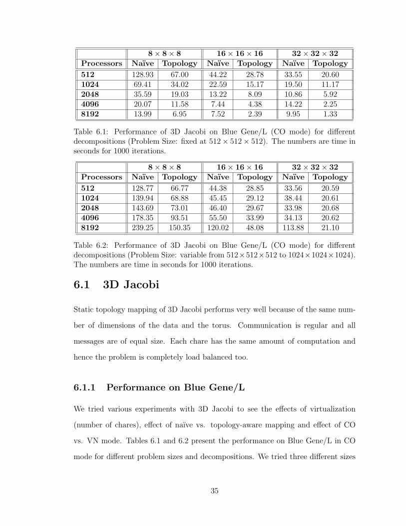
6.1 Performance of 3D Jacobi on Blue Gene/L (CO mode) for differentdecompositions (Problem Size: fixed at 512×512×512). The numbersare time in seconds for 1000 iterations. . . . . . . . . . . . . . . . . . 35

6.2 Performance of 3D Jacobi on Blue Gene/L (CO mode) for differentdecompositions (Problem Size: variable from 512×512×512 to 1024×1024× 1024). The numbers are time in seconds for 1000 iterations. . 35

6.3 Performance and hop-counts for 3D Jacobi on Blue Gene/L (VNmode) for block size 32 × 32 × 32 (Problem Size: fixed at 512 ×512× 1024). The numbers are time in seconds for 1000 iterations. . . 37

6.4 Performance and hop-counts for 3D Jacobi on Cray XT3 for differentdecompositions (Problem Size: fixed at 512 × 512 × 512). N standsfor naıve and T stands for topology-aware mapping. The numbersare time in seconds for 1000 iterations. . . . . . . . . . . . . . . . . . 38

6.5 Performance and hop-counts for 3D Jacobi on Cray XT3 for differentdecompositions (Problem Size: variable from 512×512×256 to 1024×512 × 1024). N stands for naıve and T stands for topology-awaremapping. The numbers are time in seconds for 1000 iterations. . . . . 38

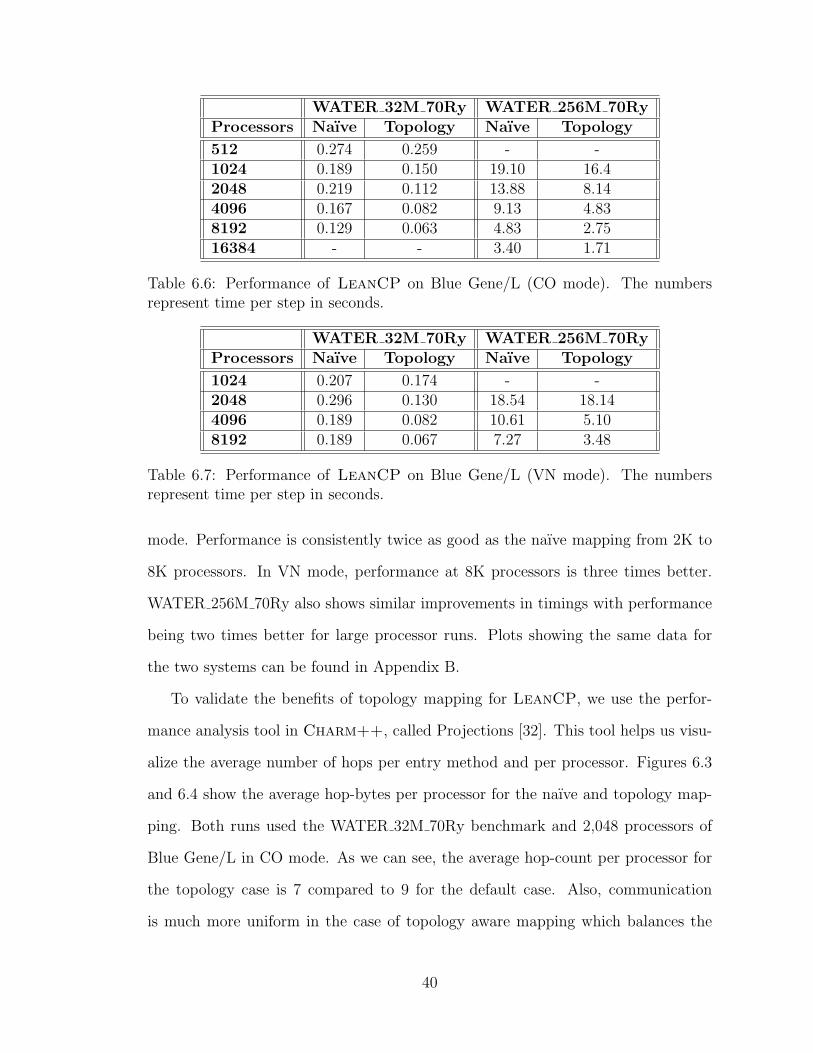
6.6 Performance of LeanCP on Blue Gene/L (CO mode). The numbersrepresent time per step in seconds. . . . . . . . . . . . . . . . . . . . 40

6.7 Performance of LeanCP on Blue Gene/L (VN mode). The numbersrepresent time per step in seconds. . . . . . . . . . . . . . . . . . . . 40

6.8 Reduction in hop-bytes for 3D NAMD on Blue Gene/L (Bench-mark:ApoA1) . . . . . . . . . . . . . . . . . . . . . . . . . . . . . . . 42

6.9 Reduction in hop-bytes for 3D NAMD on Blue Gene/L (Benchmark:F1-ATPase) . . . . . . . . . . . . . . . . . . . . . . . . . . . . . . . . . . 42

ix

List of Figures

1.1 A three-dimensional torus network (All connections are not shownfor the sake of simplicity) . . . . . . . . . . . . . . . . . . . . . . . . . 2

2.1 (a) A 2-dimensional mesh network, (b) A 2-dimensional torus network 72.2 A 4-dimensional hypercube network . . . . . . . . . . . . . . . . . . . 7

3.1 Programmer’s and System’s view of the same program under execution 123.2 Topology-aware mapping of 3D Jacobi’s data array onto the 3D pro-

cessor grid. Different colors (shades) signify which chares get mappedto which processors . . . . . . . . . . . . . . . . . . . . . . . . . . . . 16

3.3 Hop-count measurement for 3D Jacobi running on Blue Gene/L (us-ing one processor per node) . . . . . . . . . . . . . . . . . . . . . . . 17

4.1 Flow of control in LeanCP . . . . . . . . . . . . . . . . . . . . . . . 204.2 Mapping of different arrays to the 3D torus of the machine . . . . . . 24

5.1 Communication between patches and other objects in NAMD . . . . 285.2 Computes and patches mapped to the processor torus . . . . . . . . . 295.3 Choice of the best processor to place a compute. The best choice is

on the extreme left where we get two proxies on one processor. Theworst is on the right where we cannot find any proxy/patch on theprocessor. . . . . . . . . . . . . . . . . . . . . . . . . . . . . . . . . . 31

5.4 Topological search for a underloaded processor in the 3D torus . . . . 32

6.1 Performance of 3D Jacobi on Blue Gene/L (CO mode) . . . . . . . . 366.2 Hops for 3D Jacobi on Blue Gene/L (CO mode) . . . . . . . . . . . . 376.3 Average Hops for LeanCP on Blue Gene/L for the naıve mapping . . 416.4 Average Hops for LeanCP on Blue Gene/L for the topology mapping 41

8.1 Performance of 3D Jacobi on Blue Gene/L (VN mode) . . . . . . . . 518.2 Hops for 3D Jacobi on Blue Gene/L (VN mode) . . . . . . . . . . . . 518.3 Performance of 3D Jacobi on Cray XT3 . . . . . . . . . . . . . . . . . 528.4 Hops for 3D Jacobi on Cray XT3 . . . . . . . . . . . . . . . . . . . . 52

9.5 Performance of LeanCP using the WATER 32M 70Ry benchmark onBlue Gene/L . . . . . . . . . . . . . . . . . . . . . . . . . . . . . . . 53

9.6 Performance of LeanCP using the WATER 256M 70Ry benchmarkon Blue Gene/L . . . . . . . . . . . . . . . . . . . . . . . . . . . . . . 53

x

List of Abbreviations

NAMD Nanoscale Molecular Dynamics

CPAIMD Car-Parrinello ab-initio Molecular Dynamics

PPL Parallel Programming Laboratory

IBM International Business Machines

PSC Pittsburgh Supercomputing Center

3D 3-dimensional

VP Virtual Processor

PE Physical Processor

2D 2-dimensional

et al. et alii (and others)

RTS runtime system

1D 1-dimensional

6D 6-dimensional

API Application Programming Interface

a.k.a. also known as

FFT Fast Fourier Transform

4D 4-dimensional

MD Molecular Dynamics

etc. et cetera

PME Particle Mesh Ewald

ORB Orthogonal Recursive Bisection

xi

BG/L Blue Gene/L

CO co-processor mode

VN virtual node mode

vs. versus

ApoA1 Apolipoprotein-A1

F1-ATPase Adenosine Triphosphate Synthase

xii

List of Symbols

Λ overlap matrix Lambda

Ψ overlap matrix Psi

G(,) GSpace

ns number of states

Ng number of planes in g-space

N number of planes

Ngρ number of density points in g-space

Ny number of sub-planes

natom−type types of atoms

R(,) RealSpace

Gρ() RhoG

Rρ(,) RhoR

P(,,,,) PairCalculator

Ry Rydberg

MHz Megahertz

MB Megabyte

GHz Gigahertz

GB Gigabyte

A Angstrom

xiii

1 Introduction

Computation and communication are the two aspects of a parallel program which

decide its efficiency and performance. Computation needs to be divided evenly

among processors to achieve perfect load balance. Communication on the other

hand needs to be minimized across processors to ensure minimum overhead. These

two tasks are not independent of each other and need to be performed together.

To minimize communication, we need to place communicating objects on the

same physical processor. This might not be feasible always if we wish to avoid

overloading a particular processor with computational work. In such cases, com-

municating objects should be placed on processors which are close in terms of the

number of network links a message has to travel to go from one to the other. This

might not be possible for irregular or flat topologies but is possible for clearly defined

three-dimensional (3D) topologies. Let us look at a few of them and analyze how

information about such topologies can be utilized to our benefit during a program

run.

1.1 Parallel Machines and Topologies

Most supercomputers today have their processors connected through a multi-dimensional

interconnect network. The network can be a 3D mesh, a 3D torus or a butterfly or

fat-tree network or something different. New supercomputers might have complex

topologies which are a hybrid of simple ones. We need to understand the topology

of the machine to map objects onto physical processors effectively.

1

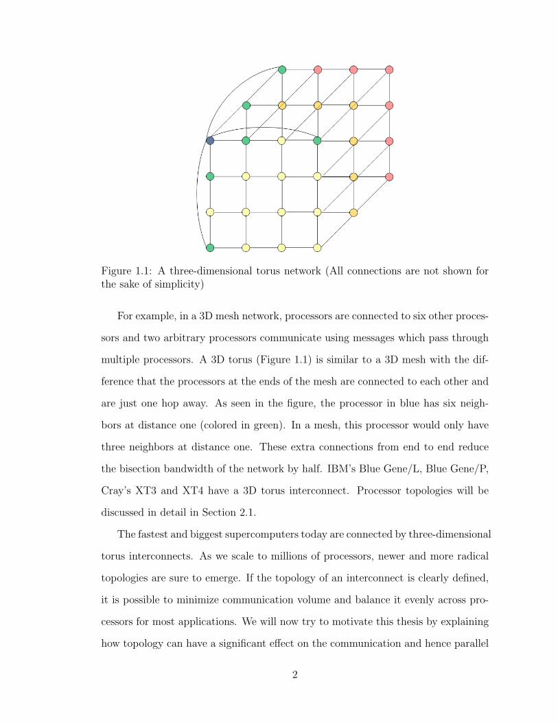
Figure 1.1: A three-dimensional torus network (All connections are not shown forthe sake of simplicity)

For example, in a 3D mesh network, processors are connected to six other proces-

sors and two arbitrary processors communicate using messages which pass through

multiple processors. A 3D torus (Figure 1.1) is similar to a 3D mesh with the dif-

ference that the processors at the ends of the mesh are connected to each other and

are just one hop away. As seen in the figure, the processor in blue has six neigh-

bors at distance one (colored in green). In a mesh, this processor would only have

three neighbors at distance one. These extra connections from end to end reduce

the bisection bandwidth of the network by half. IBM’s Blue Gene/L, Blue Gene/P,

Cray’s XT3 and XT4 have a 3D torus interconnect. Processor topologies will be

discussed in detail in Section 2.1.

The fastest and biggest supercomputers today are connected by three-dimensional

torus interconnects. As we scale to millions of processors, newer and more radical

topologies are sure to emerge. If the topology of an interconnect is clearly defined,

it is possible to minimize communication volume and balance it evenly across pro-

cessors for most applications. We will now try to motivate this thesis by explaining

how topology can have a significant effect on the communication and hence parallel

2

performance of a program.

1.2 Effect of Topology on Communication

Without a knowledge of the topology of a machine, we would place entities of a par-

allel program arbitrarily. However, this might lead to unoptimized communication

among the entities. If we can co-locate communicating objects close to each other

on nearby processors, we can minimize communication volume.

Communication volume is characterized by hop-bytes [1] which is in turn de-

pendent on the hop-count. Hop-count is the number of hops (processors) through

which a message has to jump to go from one processor to another. Hop-bytes

are obtained by multiplying the hop-count for a message by its message size. The

sum of hop-bytes for all messages for a program gives us its total communication

volume. Ideally we want all communication to be local to each processor so that

this volume is zero. However this is not possible in many scenarios (for example,

if there is all-to-all communication). Hence, we aim at minimizing this volume by

placing communicating objects on nearby processors.

To achieve the above-mentioned effect, we require two kinds of information dur-

ing the actual program run: 1. communication graph of the parallel entities in

a program and, 2. topology information about the processors being used on the

particular machine. This bring us to the choice of a parallel language which helps

us express both easily. The parallel language and framework used in this thesis

is Charm++. We now introduce Charm++ and some applications written in

Charm++ which are used in this work for implementation of the ideas and algo-

rithms, and for obtaining results.

3

1.3 Charm++ and its Applications

The Charm++ [2, 3] parallel language and runtime system is based on an object-

oriented parallel programming model. Charm++ is message-driven and based on

the idea of virtualization. Virtualization is the idea of decomposing a problem into a

large number of small parts where this number is generally a lot more than the num-

ber of processors. Mapping these small parts (virtual processors or VPs) to physical

processors (PEs) leads to an adaptive overlap of computation and communication.

It also provides us with a framework for obtaining the communication properties

of the application and flexibility of mapping VPs to PEs. This framework will be

discussed in Chapter 3.

As a proof of principle, to demonstrate the effectiveness of topology mapping, we

use a simple application written in Charm++. It is a 7-point 3-dimensional stencil

(referred to as 3D Jacobi henceforth in this thesis) which does regular communica-

tion with its neighbors. The two real applications which have benefitted from the

research in this thesis are NAMD and LeanCP. NAMD [4, 5] is a classical molecu-

lar dynamics application which involves calculation of forces and velocities of atoms

in a system. It has both migratable (objects that can be moved across processors)

and non-migratable (objects which stay on a fixed processor during the entire run)

objects. NAMD does an initial assignment of the non-migratable objects. The mi-

gratable objects are assigned by a load balancer to the processors which is critical

for good performance. In this thesis, we look at the benefits of topological placement

of these migratable objects close to their interacting non-migratable counterparts.

LeanCP [6, 7] is a quantum chemistry application also written in Charm++. It

is an implementation of the Car-Parrinello ab initio molecular dynamics (CPAIMD)

algorithm. LeanCP has several arrays of objects which communicate in a disci-

plined fashion among their own members and with members of other arrays. This

4

gives us a fairly regular communication graph which should be relatively easy to

map on to a processor topology. But there are complex intertwined dependencies

among these objects which make this problem difficult. We try to map communi-

cating objects of the same array close to one another and also to other array objects

which are involved.

Further chapters in this thesis are organized as follows: We begin with a descrip-

tion of processor topologies and role of communication in a program in Chapter 2.

We discuss different communication scenarios and analyze which ones can be op-

timized in certain ways. We also list some of the previous work in this area. We

then move on to describe the Charm++framework in Chapter 3. Here we discuss

Charm++arrays and how they are mapped. We also discuss the topology inter-

face which provides information about the machine and the allocated partition at

runtime. 3D Jacobi is discussed in Section 3.4. Topology aware mapping for this

application is also discussed there. Chapters 4 and 5 discuss the ideas implemented

in LeanCP and NAMD respectively to improve their performance. Results which

prove and exemplify the effectiveness of topology-awareness are presented in Chap-

ter 6 and future work is discussed in Chapter 7.

5

2 Processor and CommunicationGraphs

To set the context for our work, we discuss the common processor and communi-

cation graphs which we come across nowadays. The most powerful supercomputers

today are connected by a 3D torus interconnect network. However, parallel ma-

chines can have different kinds of interconnect topologies ranging from fat-tree to

hypercube networks. Communication graphs can range from most general unstruc-

tured kind to very specific regular ones. It is important to understand different

communication scenarios to do hop-count calculations and optimize the mapping

algorithms.

2.1 Processor Topologies

Processors in a parallel machine are connected physically in some fashion. These

connections decide the topology of the interconnect joining them. We are going to

omit a discussion of networks like crossbar switching and bus networks which do

not scale to machines with thousands of processors. Below is a description of the

common topologies used in machines today:

n-Dimensional Mesh In a n-dimensional mesh network, each processor is con-

nected to two other processors in each physical dimension. This gives a total

of 2n connections for each processor. The most common case is n = 3 which is

called a 3D mesh. If the size of the mesh in each dimension is N , the diameter

of the mesh is 3 × (N − 1). Figure 2.1 (a) shows a 2-dimensional (2D) mesh

network.

6

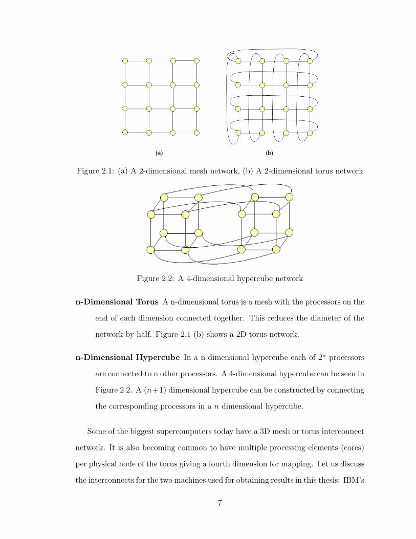
Figure 2.1: (a) A 2-dimensional mesh network, (b) A 2-dimensional torus network

Figure 2.2: A 4-dimensional hypercube network

n-Dimensional Torus A n-dimensional torus is a mesh with the processors on the

end of each dimension connected together. This reduces the diameter of the

network by half. Figure 2.1 (b) shows a 2D torus network.

n-Dimensional Hypercube In a n-dimensional hypercube each of 2n processors

are connected to n other processors. A 4-dimensional hypercube can be seen in

Figure 2.2. A (n+1) dimensional hypercube can be constructed by connecting

the corresponding processors in a n dimensional hypercube.

Some of the biggest supercomputers today have a 3D mesh or torus interconnect

network. It is also becoming common to have multiple processing elements (cores)

per physical node of the torus giving a fourth dimension for mapping. Let us discuss

the interconnects for the two machines used for obtaining results in this thesis: IBM’s

7

Blue Gene/L and Cray XT3. Blue Gene/L has a 3D torus interconnect [8]. Each

midplane (512 nodes) of the machine is a complete torus of dimension 8 × 8 × 8.

Midplanes when joined together form bigger toruses. Each node has two processors

giving rise to 1024 processors in a single midplane. Blue Gene/P has a similar

network configuration but it has 4 processors per node. This gives 2,048 processors

in a single midplane.

Cray XT3 processors are connected by a proprietary SeaStar 3D mesh intercon-

nect [9]. It is also reconfigurable as a 3D torus interconnect but only when using

the entire machine. Any smaller subset gives us a 3D mesh. It is also different in

the sense that all dimensions of the torus are different and not even. The size of the

torus on the Cray XT3 at PSC (called BigBen) is 11 × 12 × 16 in the X, Y and Z

dimensions.

2.2 Communication Scenarios

We now proceed to discuss different communication scenarios which occur in bench-

marks and real-life applications and then explain the ones which we will concentrate

upon in this thesis.

2.2.1 Regular and Irregular Communication

Based on whether each object interacts with a fixed number or variable number of

objects, we can classify the cases into:

1. Regular Communication: In this case, each object communicates with a

fixed number of objects. Let us consider the example of a 2D stencil where

each element in the array is updated by using values from four of its neigh-

bors. For this benchmark, it is known that at every step, each element will

communicate with four other elements. Such cases are the most simple and

8

easy to pin down to physical processors in a topological fashion. The appli-

cation LeanCP is also an example of the same category because each array

element communicates with a fixed number of objects which can be identified

by analyzing the algorithm.

2. Irregular Communication: It often happens that the application changes

the properties of the communicating objects which in turn changes the objects

they communicate with. For example, in a molecular dynamics application,

atoms migrate to newer objects and hence the communicating neighbors of

both the old and the new object change. Such a scenario is referred to as

irregular communication.

2.2.2 Point-to-Point, Multicasts and Reductions

Based on the degree of communication which essentially refers to if data is being sent

to/by multiple objects or data is being sent on a one-to-one basis, we can classify

the scenarios into:

1. Point-to-point Communication: When objects communicate with each

other by sending one-on-one messages, it is referred to as point-to-point com-

munication. It is fairly straightforward to understand and map the communi-

cation graph in this case.

2. Multicasts: When an object sends the same data to different objects, then it

is said to be performing a multicast. Broadcast is a special case of multicast

where the message is sent to all the objects in a program. Information about

multicasts helps in doing optimizations and minimizing communication. For

example, in most cases a multicast can be done through a tree. This does not

reduce the number of messages but reduces the load on a particular object

and hence contention around a particular processor.

9

3. Reductions: In this case also multiple objects are involved but the phe-

nomenon observed is just the opposite of what happens in a multicast. Several

objects send data to one object which collects all this data and manipulates

it further.

For the applications we are going to consider in this thesis, we will encounter all

the scenarios mentioned above. 3D Jacobi is an example of simple, regular point-

to-point communication. In LeanCP, communication is regular but we have point-

to-point messages, multicasts and reductions. NAMD has irregular communication

and also uses point-to-point messages, multicasts and reductions.

2.3 Previous Work

There has been substantial research on the general problem of mapping a com-

munication graph to a processor graph. The problem has been shown to be NP-

complete [10, 11, 12] and so efforts have been made in two directions to conquer

it: heuristic algorithms and physical optimization techniques. As early as 1981,

Bokhari [10] came up with an algorithm of pairwise exchanges to reduce interpro-

cessor communication. Results were shown for a specific array processor (the finite

element machine). Lee and Aggarwal [11] came up with a greedy algorithm which

used initial assignment and pairwise exchange. Results were presented for a 8-node

and 16-node hypercube system graph.

Physical optimization techniques like simulated annealing and genetic algorithms

have also been used. Bollinger and Midkiff [13] propose a two-phase annealing

approach to schedule traffic along network links. Arunkumar and Chockalingam [14]

propose a genetic approach which combines the benefits of global search algorithms

with local search heuristics. They claim to improve upon the genetic algorithms

in terms of the mappings produced and the time taken to obtain them which is

10

generally large in such cases. An interesting idea to reduce the time taken is proposed

by Mansour et. al [15] where graph contraction and then interpolation are used to

find solutions for large graphs.

The problem has also been studied for specific topologies and/or task graphs

which comes closer to the work discussed in this thesis. Ercal et. al [16] use a recur-

sive task allocation scheme based on the Kernighan-Lin mincut bisection heuristic

for a hypercube. Agarwal et. al [1, 17] try to solve the mapping problem for pro-

cesses with persistent load patterns using load balancing for 3D torus-like topolo-

gies. Results are shown through simulation studies for two benchmarks, Jacobi and

LeanMD [18]. They also show actual results for a 2D Jacobi-like benchmark on up

to 1,000 processors of Blue Gene/L. Performance improvement is about two times

compared to a random mapping. In this thesis, we present results for 3D Jacobi on

up to 16,384 processors of Blue Gene/L and 2,048 processors of Cray XT3. Per-

formance improvement is up to seven times compared to the default mapping for

some runs. In addition, we also show results for two production codes, NAMD and

LeanCP on the aforementioned machines.

In this light, it becomes important to also mention previous research done specif-

ically for optimizing task-layout on these two machines. Bhanot et. al [19] propose a

general method for optimizing task layout on the Blue Gene/L machine and present

results for two applications, SAGE and UMT2000 on up to 2,048 nodes. Another

interesting study by Weisser et. al [9] studies the performance impact of fragmen-

tation of the Cray XT3 machine by the resource allocator.

11

3 Objects in Charm++

Charm++ [2, 3, 20, 21] is an object-oriented parallel programming framework. It

includes a programming language based on C++ and an adaptive runtime system.

Charm++ is based on the idea of virtualization. Virtualization is the idea of divid-

ing the problem into multiple virtual processors (VPs) which are mapped to physical

processors (PEs) by an intelligent runtime system. The number of VPs is typically

much larger than the number of PEs (which makes the degree of virtualization

greater than one).

In the Charm++ programming model, decomposition of the problem is left to

the programmer; mapping and communication are handled by the runtime system

(RTS). The programmer decomposes the problems into objects and models commu-

nication between them as remote method invocations. Method invocation on objects

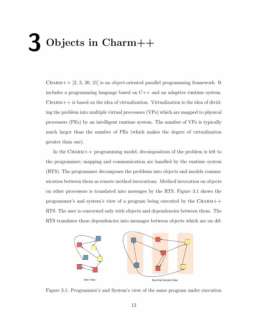
on other processors is translated into messages by the RTS. Figure 3.1 shows the

programmer’s and system’s view of a program being executed by the Charm++

RTS. The user is concerned only with objects and dependencies between them. The

RTS translates these dependencies into messages between objects which are on dif-

Figure 3.1: Programmer’s and System’s view of the same program under execution

12

ferent processors. When a remote method is invoked in Charm++ (referred to as

an “entry method”), the RTS sends a message to the concerned processor. Each

processor has a queue into which this message gets queued and is executed when

this message is processed by the scheduler. Thus, Charm++ is an asynchronous

message-driven message-passing model.

3.1 Chares and Arrays

The two most important kinds of objects in Charm++ are called Chares and Chare

Arrays. A Chare is the basic unit of computation in Charm++. It can be created

on any processor and accessed remotely (through entry methods). A Chare Array is

a collection of chares indexed by some index type. They can be considered similar to

any other arrays we come across in programming languages. We will refer to them

as chare arrays, Charm++ arrays or simply arrays interchangeably. Each element

of a chare array is called an array element. Charm++ supports 1-dimensional (1D)

to 6-dimensional (6D) arrays.

3.2 Dynamic Mapping Framework

It is important to understand how chares and chare arrays are mapped by the

RTS during a run. Charm++ does a default mapping of chares and chare arrays

to processors. For 1D arrays, it does a round-robin mapping while for 2D to 6D

arrays, it calculates a hash function using the indices and takes the remainder of

division with a big prime number (specifically, 1280107).

Charm++ provides the user with the flexibility to decide his own mapping for

an array of chares and pass it on to the RTS before array creation. The user needs

to inherit from the CkArrayMap class and override the virtual function “procNum”

13

which is called by the RTS when it is looking for the processor on which a particular

object resides. This map can be passed to the RTS when calling the constructor for

array creation.

3.3 Topology Interface in Charm++

Apart from the mapping interface, we also need information about the topology

of the machine. We need information like the dimensions of the 3D mesh/torus,

whether we have a torus (wraparound) in each dimension and functionality to get

coordinates on the torus for a processor rank and vice-versa. This was implemented

for Blue Gene/L for specific research in [22, 23], On Blue Gene/L, this information

is available in a data structure called “BGLPersonality” and can be accessed using

some system calls.

With multiple machines coming up with similar topologies, a need was felt to

make this interface more user-friendly and to hide machine-specific details from

the user. So, we implemented an API which provides the application with simple

calls to obtain information about the topology of the machine without having to

worry about the particular machine. This API now gives meaningful information

on Blue Gene/L, Cray XT3 and Blue Gene/P. The implementation details about

this interface can be found in Appendix C.

3.3.1 Cray XT3

Obtaining topology information is not straightforward on Cray XT3. There are no

system calls which can provide information about the dimensions of the partition

which has been allocated during a run. With help from technical support at Pitts-

burgh Supercomputing Center (PSC), we derived this information in several steps.

Every node on the XT3 has a unique node ID. A static routing table is available

14

on the machine which has the physical coordinates and neighbors for every node.

The Charm++ RTS reads this file during program start-up. To get the physical

coordinates corresponding to a processor rank, we obtain the node ID for the rank

through a system call and then get the coordinates from the routing table. Once we

have the coordinates for all processors in an allocation, we can get the dimensions

of the torus by looking at its diagonally opposite corners.

3.4 3D Jacobi

We begin with the first application which has been used in this thesis to demonstrate

the benefit from topology-aware mapping. 3D Jacobi is an implementation of a 3-

dimensional 7-point stencil in Charm++. We have a three dimensional array of

doubles. All elements are initialized with non-zero values. In every iteration, each

element of the array updates itself by computing the average of its six neighbors

(two in each dimension) and itself.

To parallelize the computation using Charm++, we create a 3D chare array.

Each element of this chare array is responsible for the computation of some contigu-

ous elements of the data array. The data array is divided into smaller 3D partitions

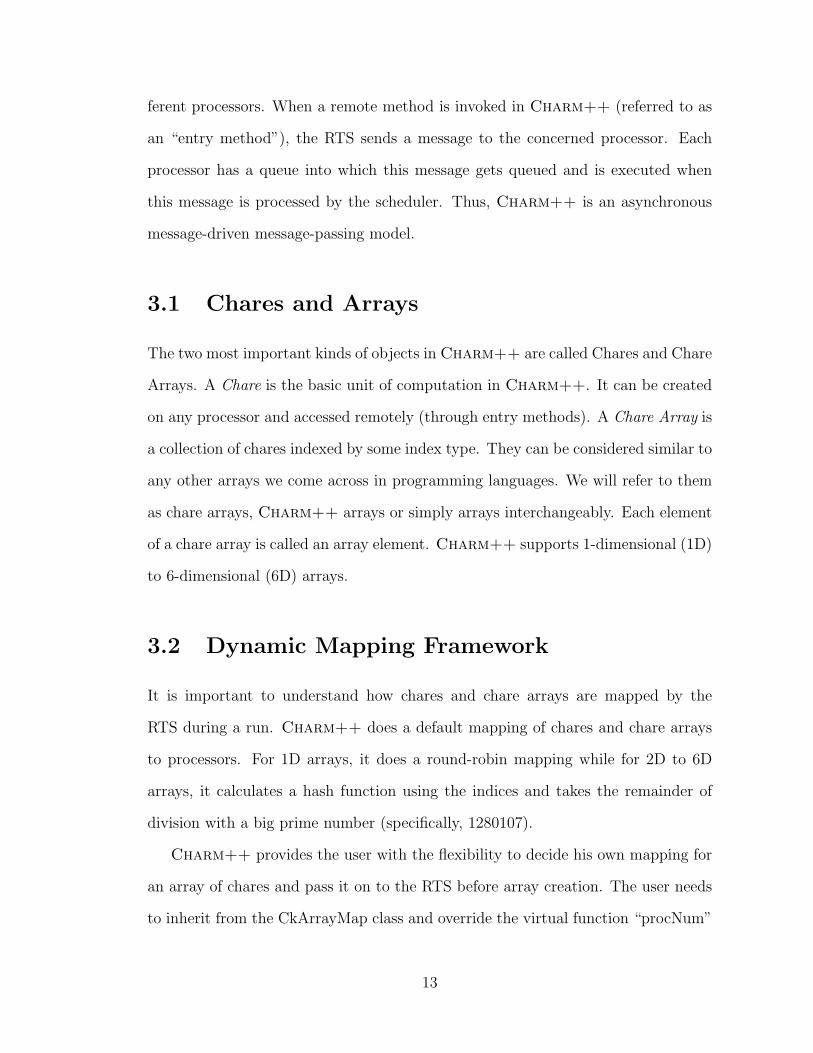
and nearby elements on the chare array get nearby 3D boxes (Figure 3.2). These

chares communicate with their neighbors to exchange the updated data on the

boundaries. Let us now see the mapping of these chares onto processors.

3.4.1 Topology Aware Mapping

The Charm++ runtime does the mapping of virtual processors to physical proces-

sors by default. Henceforth, we will refer to this mapping as the naıve or default

mapping. The RTS has no knowledge of the topology of the machine by itself and

so its mapping is totally oblivious to the communication in the application and the

15

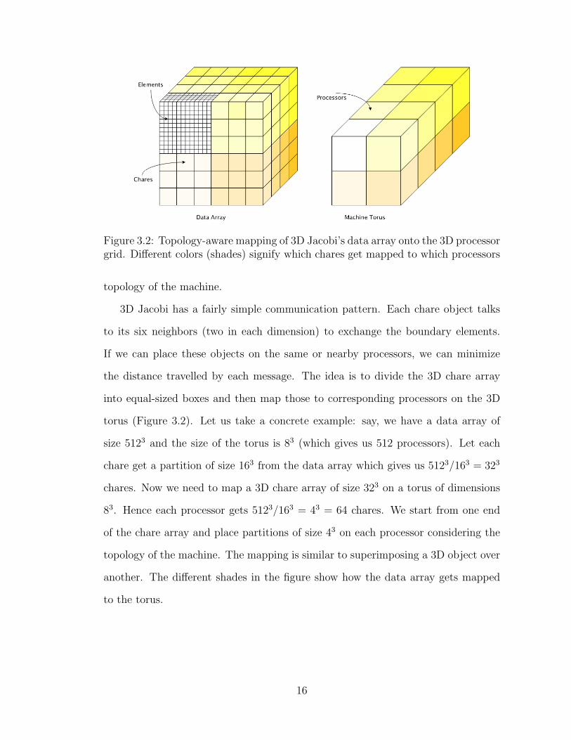
Figure 3.2: Topology-aware mapping of 3D Jacobi’s data array onto the 3D processorgrid. Different colors (shades) signify which chares get mapped to which processors

topology of the machine.

3D Jacobi has a fairly simple communication pattern. Each chare object talks

to its six neighbors (two in each dimension) to exchange the boundary elements.

If we can place these objects on the same or nearby processors, we can minimize

the distance travelled by each message. The idea is to divide the 3D chare array

into equal-sized boxes and then map those to corresponding processors on the 3D

torus (Figure 3.2). Let us take a concrete example: say, we have a data array of

size 5123 and the size of the torus is 83 (which gives us 512 processors). Let each

chare get a partition of size 163 from the data array which gives us 5123/163 = 323

chares. Now we need to map a 3D chare array of size 323 on a torus of dimensions

83. Hence each processor gets 5123/163 = 43 = 64 chares. We start from one end

of the chare array and place partitions of size 43 on each processor considering the

topology of the machine. The mapping is similar to superimposing a 3D object over

another. The different shades in the figure show how the data array gets mapped

to the torus.

16

NaiveTopology

0

100,000

200,000

300,000

400,000

500,000

600,000

700,000

800,000

512 1,024 2,048 4,096 8,192

Ho

p−

co

un

t

No. of processors

3D Jacobi with block size 32 x 32 x 32

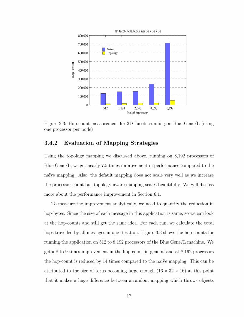
Figure 3.3: Hop-count measurement for 3D Jacobi running on Blue Gene/L (usingone processor per node)

3.4.2 Evaluation of Mapping Strategies

Using the topology mapping we discussed above, running on 8,192 processors of

Blue Gene/L, we get nearly 7.5 times improvement in performance compared to the

naıve mapping. Also, the default mapping does not scale very well as we increase

the processor count but topology-aware mapping scales beautifully. We will discuss

more about the performance improvement in Section 6.1.

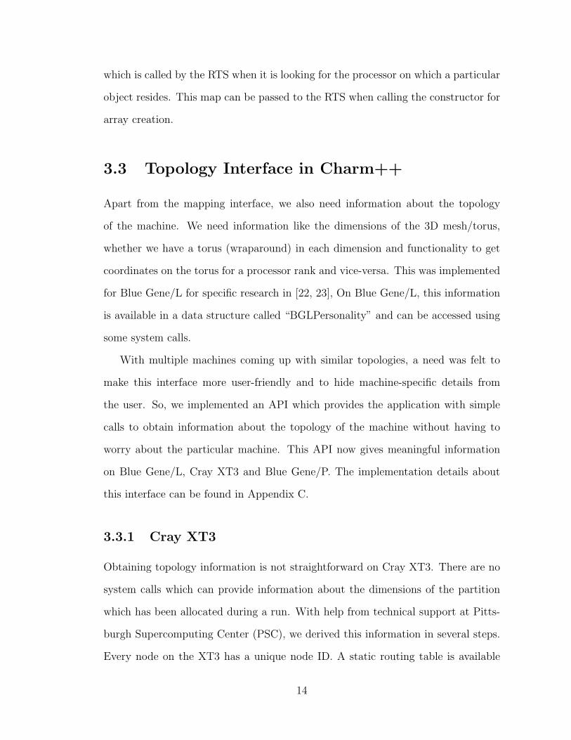
To measure the improvement analytically, we need to quantify the reduction in

hop-bytes. Since the size of each message in this application is same, so we can look

at the hop-counts and still get the same idea. For each run, we calculate the total

hops travelled by all messages in one iteration. Figure 3.3 shows the hop-counts for

running the application on 512 to 8,192 processors of the Blue Gene/L machine. We

get a 8 to 9 times improvement in the hop-count in general and at 8,192 processors

the hop-count is reduced by 14 times compared to the naive mapping. This can be

attributed to the size of torus becoming large enough (16 × 32 × 16) at this point

that it makes a huge difference between a random mapping which throws objects

17

all over the torus and a topology-aware mapping.

For the topology scheme used above, it is fairly easy to calculate the number of

hops mathematically. Let us say, we have a chare array of size N3 and processor

torus of size P 3. This gives a chare array of size N3/P 3 = C3 on each processor.

Within this C ×C ×C box of chares, the only chares that communicate externally

are the ones on the surface (on the faces, edges and corners). Each processor sends

one message per chare on the face, one more for the chares on the edges and a third

one for the chares on the corners. Hence total number of messages per processor

= (C− 2) ∗ (C− 2) ∗ 6 + (C− 2) ∗ 8 ∗ 2 + 8 ∗ 3a. For the example above, we have 323

chares on 83 processors which means 43 chares per processor. Thus each processor

has a box of 4 × 4 × 4 chares. Hence number of messages sent by each processor

every iteration is 4×6+2×8×2+8×3 = 80. This gives a total of 512×80 = 40960

hops per iteration.

18

4 LeanCP and RegularCommunication

An accurate understanding of phenomena occurring at the quantum scale can be

achieved by considering a model representing the electronic structure of the atoms

involved. The Car-Parrinello ab initio Molecular Dynamics (CPAIMD) method [24,

25, 26, 27] is one such algorithm which has been widely used to study systems con-

taining 10 − 103 atoms. The implementation of CPAIMD in Charm++ is called

LeanCP [6, 7] (a.k.a. OpenAtom, which is the name it will bear after its produc-

tion release). To achieve a fine-grained parallelization of CPAIMD, computation in

LeanCP is divided into a large number of virtual processors which enables scaling to

tens of thousands of processors. We will look at the parallel implementation of this

technique, understand its computational phases and the communication involved

and then analyze the benefit from topology-aware mapping of its objects.

4.1 Parallel Implementation

In an ab-initio approach, the system is driven by electrostatic interactions between

the nuclei and electrons. Calculating the electrostatic energy involves computing

several terms: (1) quantum mechanical kinetic energy of non-interacting electrons,

(2) Coulomb interaction between electrons or the Hartree energy, (3) correction

of the Hartree energy to account for the quantum nature of the electrons or the

exchange-correlation energy, and (4) interaction of electrons with atoms in the sys-

tem or the external energy. Hence, CPAIMD computations involve a large number

of phases (Figure 4.1) with high interprocessor communication. These phases are

19

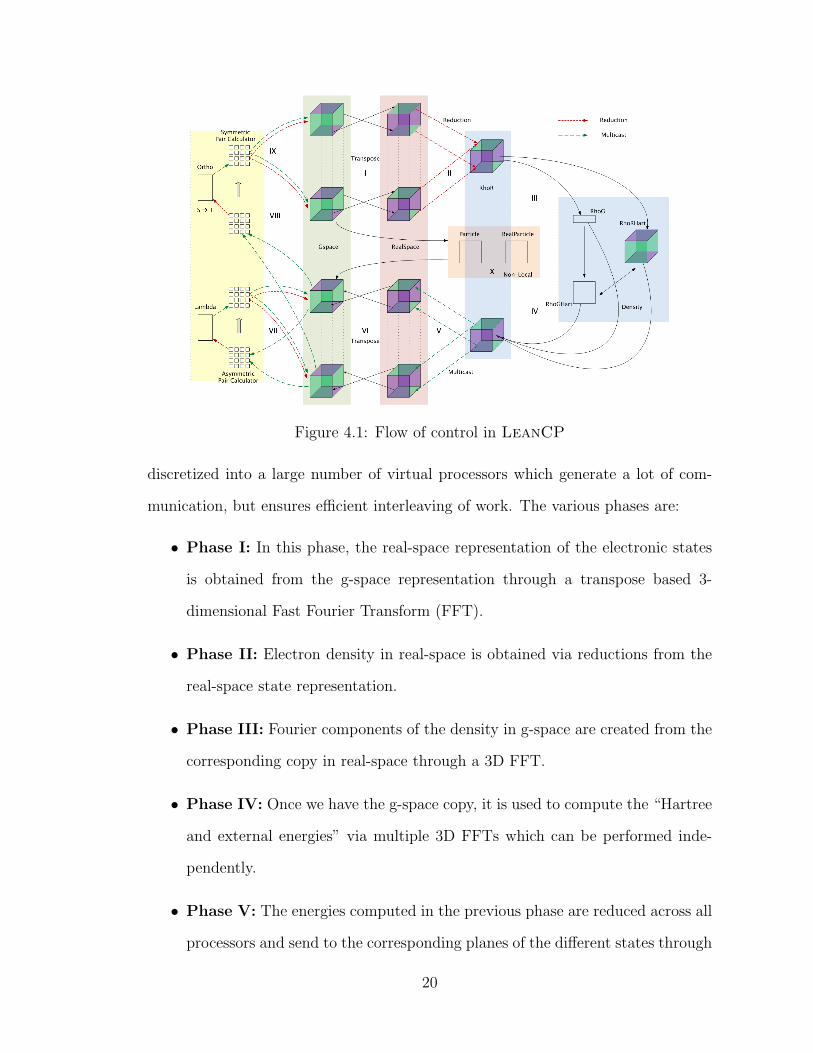
Figure 4.1: Flow of control in LeanCP

discretized into a large number of virtual processors which generate a lot of com-

munication, but ensures efficient interleaving of work. The various phases are:

• Phase I: In this phase, the real-space representation of the electronic states

is obtained from the g-space representation through a transpose based 3-

dimensional Fast Fourier Transform (FFT).

• Phase II: Electron density in real-space is obtained via reductions from the

real-space state representation.

• Phase III: Fourier components of the density in g-space are created from the

corresponding copy in real-space through a 3D FFT.

• Phase IV: Once we have the g-space copy, it is used to compute the “Hartree

and external energies” via multiple 3D FFTs which can be performed inde-

pendently.

• Phase V: The energies computed in the previous phase are reduced across all

processors and send to the corresponding planes of the different states through

20

multicasts. This is exactly reverse of the procedure used to obtain the density

in phase II.

• Phase VI: In this phase, the forces are obtained in g-space from real-space

via a 3D FFT.

• Phase VII: For functional minimization, force regularization is done in this

phase by computing the overlap matrix Lambda (Λ) and applying it. This

involves several multicasts and reductions.

• Phase VIII: This phase is similar to Phase VII and involves computation

of the overlap matrix Psi (Ψ) and its inverse square root (referred to as the

S → T process) to obtain “reorthogonalized” states. This phase is called

orthonormalization.

• Phase IX: The inverse square matrix from the previous phase is used in a

“backward path” to compute the necessary modification to the input data.

This again involves multicasts and reductions to obtain the input for phase I

of the next iteration.

• Phase X: Since Phase V is a bottleneck, this phase is interleaved with it

to perform the non-local energy computation. It involves computation of the

kinetic energy of the electrons and computation of the non-local interaction

between electrons and the atoms using the EES method [28].

For a detailed description of this algorithm please refer to [7]. We will now

proceed to understand the communication involved in these phases through a de-

scription of the various chare arrays involved and dependencies among them.

21

4.2 Communication in LeanCP

The ten phases described in the previous section are parallelized by decomposing

the physical system into 15 chare arrays of different dimensions (ranging between

one and four). A description of these objects and communication between them

follows:

1. GSpace and RealSpace: These represent the g-space and real-space rep-

resentations of the electronic states. They are 2-dimensional arrays with

states in one dimension and planes in the other. They are represented by

G(s, p) [ns × Ng] and R(s, p) [ns × N ] respectively. GSpace and RealSpace

interact through transpose operations in Phase I and hence all planes of one

state of GSpace interact with all planes of the same state of RealSpace. Re-

alSpace also interacts with RhoR through reductions in Phase II.

2. RhoG and RhoR: They are the g-space and real-space representations of

electron density and are 1-dimensional (1D) and 2-dimensional (2D) arrays

respectively. They are represented as Gρ(p) [Ngρ] and Rρ(p, p′) [(N/Ny)×Ny].

RhoG is obtained from RhoR in Phase III through two transposes.

3. RhoGHart and RhoRHart: RhoR and RhoG are used to compute their

Hartree and exchange energy counterparts through several 3D FFTs (in Phase

IV). This involves transposes and point-to-point communication. RhoGHart

and RhoRHart are 2D and 3D arrays represented by GHE(p, a) [NgHE ×

natom−type] and RHE(p, p′, a) [(1.4N/Ny)×Ny × natom−type].

4. Particle and RealParticle: These two 2D arrays are the g-space and real-

space representations of the non-local work and denoted as Gnl(s, p) [ns×Ng]

and Rnl(s, p) [ns × 0.7N ]. Phase X for the non-local computation can be

overlapped with Phases II-VI and involves communication for two 3D FFTs.

22

5. Ortho and CLA Matrix: The 2D ortho array, O(s, s′) does the post-

processing of the overlap matrices to obtain the T-matrix from the S-matrix.

There are three 2D CLA Matrix instances used in each of the steps of the

inverse square method (for matrix multiplications) used during orthonormal-

ization. In the process, these arrays communicate with the paircalculator chare

arrays mentioned next.

6. PairCalculators: These 4-dimensional (4D) arrays are used in the force reg-

ularization and orthonormalization phases (VII and VIII). They communicate

with the GSpace, CLA Matrix and Ortho arrays through multicasts and reduc-

tions. They are represented as Pc(s, s′, p, p′) of dimensions Ns×Ns×Ng×N ′g.

A particular state of the GSpace array interacts with all elements of the pair-

calculator array which have this state in one of its first two dimensions.

7. Structure Factor: This is a 3D array used when we do not use the EES

method for the non-local computation.

4.3 Topology Aware Mapping

LeanCP provides us with a scenario where the load on each virtual processor is

static (under the CPAIMD method) and the communication is regular and clearly

understood. Hence, it should be fairly straightforward to intelligently map the

arrays in this application to minimize inter-processor communication and keep load

balanced. As discussed in Chapter 3, Charm++ does a default mapping of objects

(elements of chare arrays) to processors. Let us see how we can do better than the

default mapping by using the communication and topology information at runtime.

We begin with the two most important arrays in LeanCP which represent electronic

states in g-space and real-space.

23

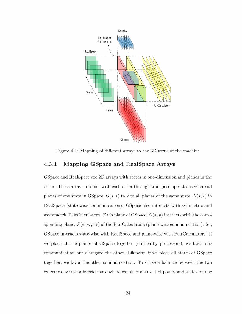
Figure 4.2: Mapping of different arrays to the 3D torus of the machine

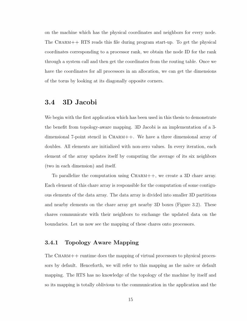
4.3.1 Mapping GSpace and RealSpace Arrays

GSpace and RealSpace are 2D arrays with states in one-dimension and planes in the

other. These arrays interact with each other through transpose operations where all

planes of one state in GSpace, G(s, ∗) talk to all planes of the same state, R(s, ∗) in

RealSpace (state-wise communication). GSpace also interacts with symmetric and

asymmetric PairCalculators. Each plane of GSpace, G(∗, p) interacts with the corre-

sponding plane, P (∗, ∗, p, ∗) of the PairCalculators (plane-wise communication). So,

GSpace interacts state-wise with RealSpace and plane-wise with PairCalculators. If

we place all the planes of GSpace together (on nearby processors), we favor one

communication but disregard the other. Likewise, if we place all states of GSpace

together, we favor the other communication. To strike a balance between the two

extremes, we use a hybrid map, where we place a subset of planes and states on one

24

processor.

We start with laying out the GSpace array on the torus and then map other

objects based on GSpace’s mapping. The 3D torus is divided into rectangular boxes

(which we will refer to as “prisms”) such that we get prisms equal in number to the

planes in GSpace. The longest dimension of the prism is chosen to be the same as

one of the dimensions of the torus. Within each prism for a specific plane, the states

in G(*, p) are laid out in increasing order along the long axis of the prism. Figure 4.2

shows the GSpace chares at the bottom being mapped along the long dimension of

the torus in the center. Once GSpace is mapped, we place the RealSpace chares.

We come up with prisms perpendicular to the GSpace prisms which are formed by

including processors holding all planes for a particular state of GSpace, G(s, ∗). The

corresponding states of RealSpace, R(s, ∗) are mapped on to these prisms.

4.3.2 Mapping of Density Objects

RhoR objects communicate with RealSpace plane wise and hence Rρ(p, ∗) have to

be placed close to R(∗, p). To achieve this, we start with the centroid of the prism

used by R(∗, p) and place RhoR chares in proximity to it. RhoG chares, Gρ(p) are

mapped near RhoR chares, Rρ(p, ∗) but not on the same processors as RhoR to

avoid bottlenecks.

4.3.3 Mapping PairCalculator Arrays

Since PairCalculator and GSpace chares interact plane-wise, the effort is to place

G(∗, p) and P (∗, ∗, p, ∗) together. Chares with indices P (s1, s2, p, p′) are placed

around the centroid of G(s1, p), ..., G(s1+sgrain, p) and G(s2, p), ...., G(s2+sgrain, p).

This minimizes the hop-count for orthonormalization input and output.

25

The mapping schemes discussed above substantially reduce the hop-count for dif-

ferent phases. They also restrict different communication patterns to specific prisms

within the torus, thereby reducing contention and ensuring balanced communica-

tion through out the torus. State-wise and plane-wise communication is confined to

different (orthogonal) prisms. This helps avoid scaling bottlenecks as we will see in

Section 6.2.

26

5 NAMD and Multicasts

Understanding biomolecular systems has been aided by the development of molec-

ular dynamics applications for simulation of biomolecular reactions. NAMD [4, 5,

29, 30] is a molecular dynamics code which is widely used for molecular dynamics

simulations. It was written using Charm++about ten years ago and has performed

well on a variety of machines and molecular systems. With the emergence of large

supercomputers, further optimizations have become necessary to scale NAMD to

tens of thousands of processors. Since the molecular system is a simulation box

with spatial coordinates for each atom, it should be possible to do a topological

placement of the atoms to minimize communication. Lets us look at how this is

done in NAMD.

5.1 Parallel Implementation

Classical Molecular Dynamics (MD) requires the calculation of forces due to bonds

and non-bonded forces (which include electrostatic and Van der Waal’s forces).

For parallelization, NAMD does a hybrid of spatial and force decomposition to

combine the advantages of both [31]. The simulation box is divided into patches

each containing a few atoms. For every pair of interacting patches, we create a chare

(called a compute) which is responsible for calculating the pairwise forces between

the patches. There are different kinds of computes depending on the forces they

calculate: bonded (angles, dihedrals, crossterms etc.) and non-bonded computes.

The number of patches is considerably less than the number of computes. The

27

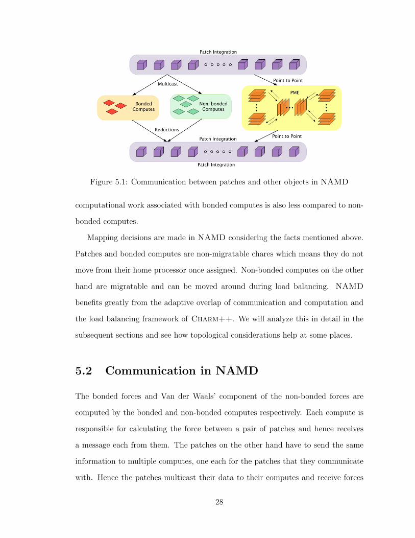
Figure 5.1: Communication between patches and other objects in NAMD

computational work associated with bonded computes is also less compared to non-

bonded computes.

Mapping decisions are made in NAMD considering the facts mentioned above.

Patches and bonded computes are non-migratable chares which means they do not

move from their home processor once assigned. Non-bonded computes on the other

hand are migratable and can be moved around during load balancing. NAMD

benefits greatly from the adaptive overlap of communication and computation and

the load balancing framework of Charm++. We will analyze this in detail in the

subsequent sections and see how topological considerations help at some places.

5.2 Communication in NAMD

The bonded forces and Van der Waals’ component of the non-bonded forces are

computed by the bonded and non-bonded computes respectively. Each compute is

responsible for calculating the force between a pair of patches and hence receives

a message each from them. The patches on the other hand have to send the same

information to multiple computes, one each for the patches that they communicate

with. Hence the patches multicast their data to their computes and receive forces

28

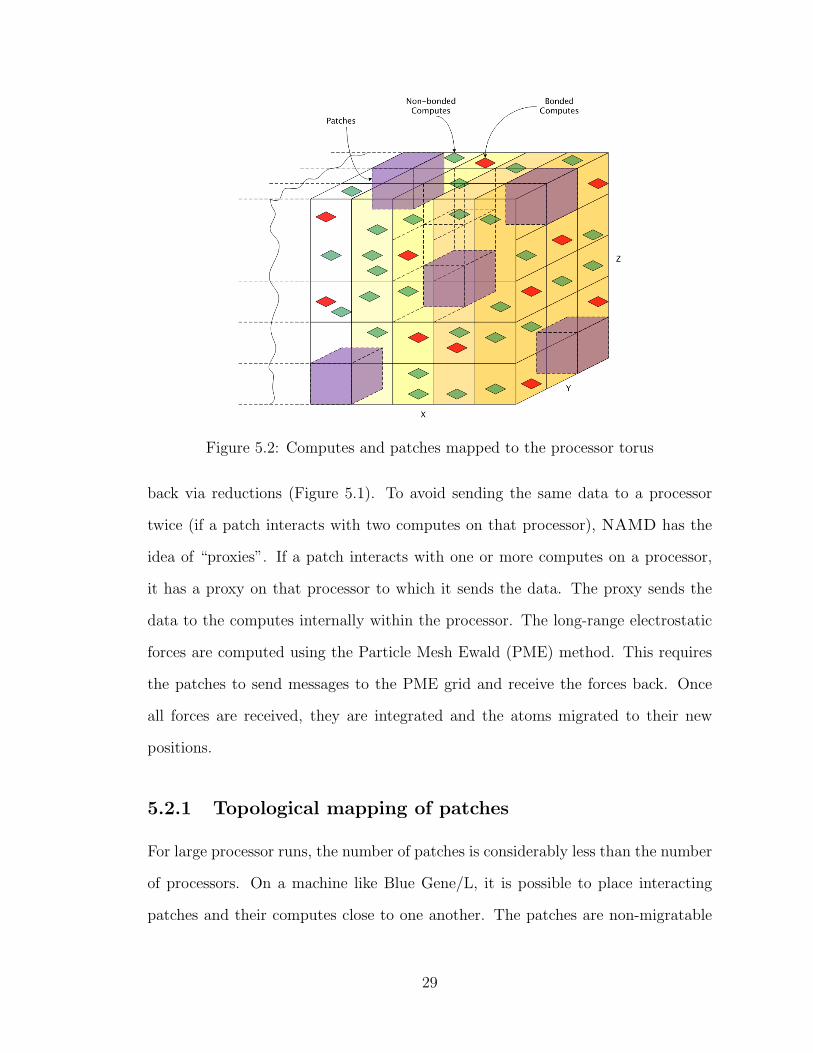
Figure 5.2: Computes and patches mapped to the processor torus

back via reductions (Figure 5.1). To avoid sending the same data to a processor

twice (if a patch interacts with two computes on that processor), NAMD has the

idea of “proxies”. If a patch interacts with one or more computes on a processor,

it has a proxy on that processor to which it sends the data. The proxy sends the

data to the computes internally within the processor. The long-range electrostatic

forces are computed using the Particle Mesh Ewald (PME) method. This requires

the patches to send messages to the PME grid and receive the forces back. Once

all forces are received, they are integrated and the atoms migrated to their new

positions.

5.2.1 Topological mapping of patches

For large processor runs, the number of patches is considerably less than the number

of processors. On a machine like Blue Gene/L, it is possible to place interacting

patches and their computes close to one another. The patches are non-migratable

29

and we need to decide an initial static mapping for them. Ideally, we would like to

place the patches maximally away so that the simulation box occupies the whole

torus and then place the computes between them.

A strategy to divide the simulation box and place it on the 3D torus of Blue

Gene/L is discussed in [22, 23]. An orthogonal recursive bisection (ORB) is done on

the 3D torus until we get partitions equal to the number of patches. Then we map

the spatially divided simulation box onto the processor partitions. Figure 5.2 shows

the mapping of patches, bonded and non-bonded computes on to the 3D torus. This

scheme has now been made general using the topology interface in Charm++ and

can now be used on any machine with topology information.

Once the patches are mapped, the non-migratable bonded computes are placed

with no topological consideration. Non-bonded computes are also placed likewise.

But these create load imbalance and hence are reshuffled soon within a major load

balancing step. We discuss the NAMD load balancers next.

5.3 Load Balancing

NAMD depends heavily on the load balancing framework provided by Charm++

for good performance. Computational load in NAMD is persistent across iterations

and hence, load information from previous iterations can be used in future iterations.

Every few hundred or thousand iterations, a few iterations are instrumented and the

load information from these steps is used during the load balancing step to unload

the overloaded processors.

There are two major load balancers at work in NAMD. The first one is a com-

prehensive load balancer which considers every compute and processor and assigns a

mapping for all the computes. This leads to movement of a lot of computes. This is

called only once, right after start-up. The second one is a refinement load balancer

30

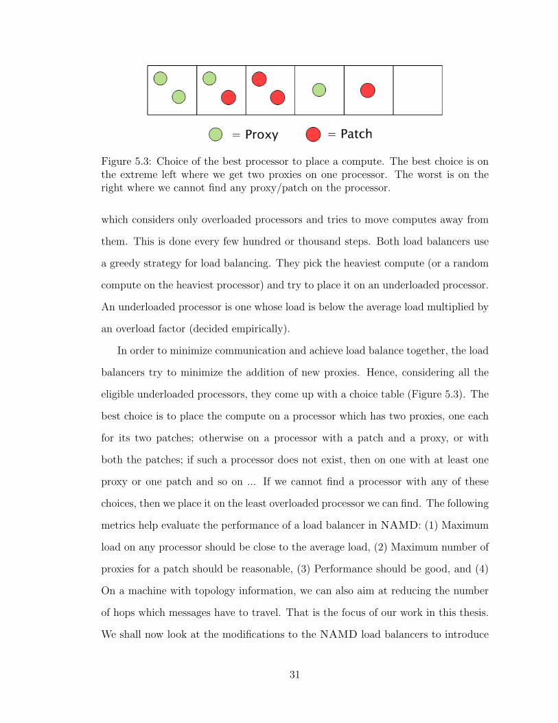
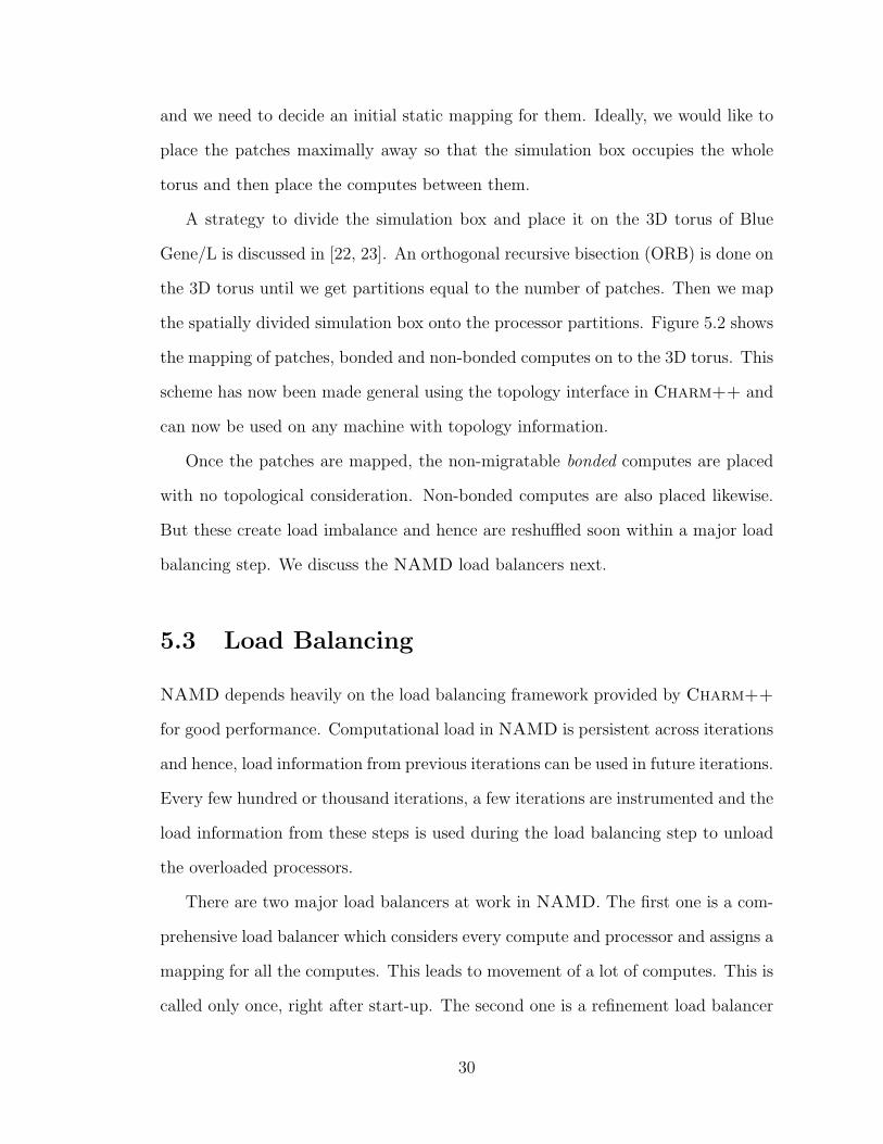
Figure 5.3: Choice of the best processor to place a compute. The best choice is onthe extreme left where we get two proxies on one processor. The worst is on theright where we cannot find any proxy/patch on the processor.

which considers only overloaded processors and tries to move computes away from

them. This is done every few hundred or thousand steps. Both load balancers use

a greedy strategy for load balancing. They pick the heaviest compute (or a random

compute on the heaviest processor) and try to place it on an underloaded processor.

An underloaded processor is one whose load is below the average load multiplied by

an overload factor (decided empirically).

In order to minimize communication and achieve load balance together, the load

balancers try to minimize the addition of new proxies. Hence, considering all the

eligible underloaded processors, they come up with a choice table (Figure 5.3). The

best choice is to place the compute on a processor which has two proxies, one each

for its two patches; otherwise on a processor with a patch and a proxy, or with

both the patches; if such a processor does not exist, then on one with at least one

proxy or one patch and so on ... If we cannot find a processor with any of these

choices, then we place it on the least overloaded processor we can find. The following

metrics help evaluate the performance of a load balancer in NAMD: (1) Maximum

load on any processor should be close to the average load, (2) Maximum number of

proxies for a patch should be reasonable, (3) Performance should be good, and (4)

On a machine with topology information, we can also aim at reducing the number

of hops which messages have to travel. That is the focus of our work in this thesis.

We shall now look at the modifications to the NAMD load balancers to introduce

31

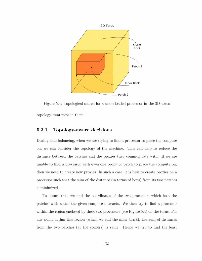
Figure 5.4: Topological search for a underloaded processor in the 3D torus

topology-awareness in them.

5.3.1 Topology-aware decisions

During load balancing, when we are trying to find a processor to place the compute

on, we can consider the topology of the machine. This can help to reduce the

distance between the patches and the proxies they communicate with. If we are

unable to find a processor with even one proxy or patch to place the compute on,

then we need to create new proxies. In such a case, it is best to create proxies on a

processor such that the sum of the distance (in terms of hops) from its two patches

is minimized.

To ensure this, we find the coordinates of the two processors which host the

patches with which the given compute interacts. We then try to find a processor

within the region enclosed by these two processors (see Figure 5.4) on the torus. For

any point within this region (which we call the inner brick), the sum of distances

from the two patches (at the corners) is same. Hence we try to find the least

32

overloaded processor within this brick.

If we fail, then we need to try the rest of the torus (called the outer brick). We

spiral around the inner brick on the outside and try to find the first underloaded

processor we can. As soon as we find one, we place the compute on it. We will see

in Section 6.3, the benefit from this optimization in terms of reduction in hop-bytes

and better performance.

33

6 Results

In this chapter, we discuss and analyze the results of the schemes developed in the

previous chapters for topology sensitive mapping and load balancing for different

applications. Results are presented for 3D Jacobi, LeanCP and NAMD on up to

16,384 processors of Blue Gene/L and 2,048 processors of Cray XT3.

A brief description of the two machines follows:

• IBM’s Blue Gene/L: The Blue Gene/L machine at IBM T J Watson (re-

ferred to as the “Watson BG/L”) has 20,480 nodes. Each node contains two

700 MHz PowerPC 440 cores and has 512 MB of memory shared between the

two. The nodes on Blue Gene/L are connected into a 3D torus. We used the

Watson BG/L for most of our runs. Blue Gene/L can be run in two modes:

co-processor or CO mode where we just use one processor per node for the

computation and virtual node or VN mode where we use both processors per

node.

• Cray’s XT3: BigBen at Pittsburgh Supercomputing Center (PSC) has 2,068

compute nodes each of which has two 2.6 GHz AMD Opteron processors. The

two processors on a node share 2 GB of memory. The nodes are connected

into a 3D torus by a custom SeaStar interconnect. We do not get a contiguous

allocation of processors on XT3 if we use the default queue. We had to take

help from the PSC staff to set up a reservation to get a mesh of 8 × 8 × 16

which is 1,024 nodes and 2,048 processors.

34

8× 8× 8 16× 16× 16 32× 32× 32Processors Naıve Topology Naıve Topology Naıve Topology

512 128.93 67.00 44.22 28.78 33.55 20.601024 69.41 34.02 22.59 15.17 19.50 11.172048 35.59 19.03 13.22 8.09 10.86 5.924096 20.07 11.58 7.44 4.38 14.22 2.258192 13.99 6.95 7.52 2.39 9.95 1.33

Table 6.1: Performance of 3D Jacobi on Blue Gene/L (CO mode) for differentdecompositions (Problem Size: fixed at 512× 512× 512). The numbers are time inseconds for 1000 iterations.

8× 8× 8 16× 16× 16 32× 32× 32Processors Naıve Topology Naıve Topology Naıve Topology

512 128.77 66.77 44.38 28.85 33.56 20.591024 139.94 68.88 45.45 29.12 38.44 20.612048 143.69 73.01 46.40 29.67 33.98 20.684096 178.35 93.51 55.50 33.99 34.13 20.628192 239.25 150.35 120.02 48.08 113.88 21.10

Table 6.2: Performance of 3D Jacobi on Blue Gene/L (CO mode) for differentdecompositions (Problem Size: variable from 512×512×512 to 1024×1024×1024).The numbers are time in seconds for 1000 iterations.

6.1 3D Jacobi

Static topology mapping of 3D Jacobi performs very well because of the same num-

ber of dimensions of the data and the torus. Communication is regular and all

messages are of equal size. Each chare has the same amount of computation and

hence the problem is completely load balanced too.

6.1.1 Performance on Blue Gene/L

We tried various experiments with 3D Jacobi to see the effects of virtualization

(number of chares), effect of naıve vs. topology-aware mapping and effect of CO

vs. VN mode. Tables 6.1 and 6.2 present the performance on Blue Gene/L in CO

mode for different problem sizes and decompositions. We tried three different sizes

35

1

2

4

8

16

32

64

128

512 1K 2K 4K 8K

Tim

e (s

econ

ds)

No. of processors

3D Jacobi with block size 32 x 32 x 32

Variable Problem NaiveVariable Problem Topology

Fixed Problem NaiveFixed Problem Topology

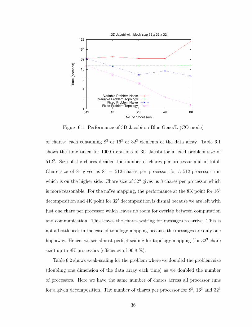
Figure 6.1: Performance of 3D Jacobi on Blue Gene/L (CO mode)

of chares: each containing 83 or 163 or 323 elements of the data array. Table 6.1

shows the time taken for 1000 iterations of 3D Jacobi for a fixed problem size of

5123. Size of the chares decided the number of chares per processor and in total.

Chare size of 83 gives us 83 = 512 chares per processor for a 512-processor run

which is on the higher side. Chare size of 323 gives us 8 chares per processor which

is more reasonable. For the naıve mapping, the performance at the 8K point for 163

decomposition and 4K point for 323 decomposition is dismal because we are left with

just one chare per processor which leaves no room for overlap between computation

and communication. This leaves the chares waiting for messages to arrive. This is

not a bottleneck in the case of topology mapping because the messages are only one

hop away. Hence, we see almost perfect scaling for topology mapping (for 323 chare

size) up to 8K processors (efficiency of 96.8 %).

Table 6.2 shows weak-scaling for the problem where we doubled the problem size

(doubling one dimension of the data array each time) as we doubled the number

of processors. Here we have the same number of chares across all processor runs

for a given decomposition. The number of chares per processor for 83, 163 and 323

36

NaiveTopology

0

100,000

200,000

300,000

400,000

500,000

600,000

700,000

800,000

512 1,024 2,048 4,096 8,192

Ho

p−

co

un

t

No. of processors

3D Jacobi with block size 32 x 32 x 32

Figure 6.2: Hops for 3D Jacobi on Blue Gene/L (CO mode)

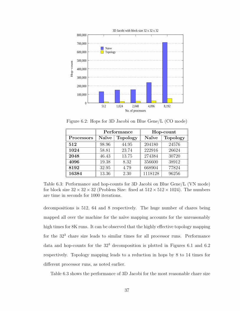
Performance Hop-countProcessors Naıve Topology Naıve Topology

512 98.96 44.95 204180 245761024 58.81 23.74 222916 266242048 46.43 13.75 274384 307204096 19.38 8.32 356600 389128192 32.95 4.79 668904 7782416384 13.36 2.30 1118128 96256

Table 6.3: Performance and hop-counts for 3D Jacobi on Blue Gene/L (VN mode)for block size 32× 32× 32 (Problem Size: fixed at 512× 512× 1024). The numbersare time in seconds for 1000 iterations.

decompositions is 512, 64 and 8 respectively. The huge number of chares being

mapped all over the machine for the naıve mapping accounts for the unreasonably

high times for 8K runs. It can be observed that the highly effective topology mapping

for the 323 chare size leads to similar times for all processor runs. Performance

data and hop-counts for the 323 decomposition is plotted in Figures 6.1 and 6.2

respectively. Topology mapping leads to a reduction in hops by 8 to 14 times for

different processor runs, as noted earlier.

Table 6.3 shows the performance of 3D Jacobi for the most reasonable chare size

37

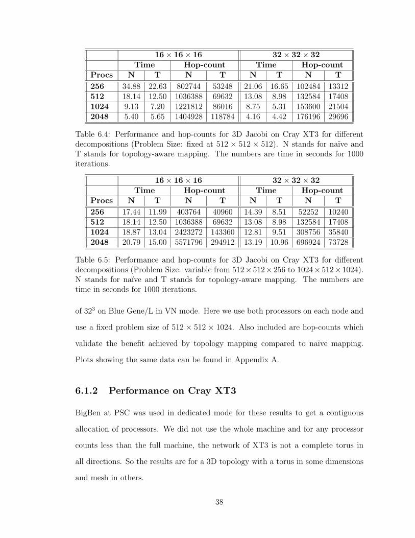
16× 16× 16 32× 32× 32Time Hop-count Time Hop-count

Procs N T N T N T N T

256 34.88 22.63 802744 53248 21.06 16.65 102484 13312512 18.14 12.50 1036388 69632 13.08 8.98 132584 174081024 9.13 7.20 1221812 86016 8.75 5.31 153600 215042048 5.40 5.65 1404928 118784 4.16 4.42 176196 29696

Table 6.4: Performance and hop-counts for 3D Jacobi on Cray XT3 for differentdecompositions (Problem Size: fixed at 512 × 512 × 512). N stands for naıve andT stands for topology-aware mapping. The numbers are time in seconds for 1000iterations.

16× 16× 16 32× 32× 32Time Hop-count Time Hop-count

Procs N T N T N T N T

256 17.44 11.99 403764 40960 14.39 8.51 52252 10240512 18.14 12.50 1036388 69632 13.08 8.98 132584 174081024 18.87 13.04 2423272 143360 12.81 9.51 308756 358402048 20.79 15.00 5571796 294912 13.19 10.96 696924 73728

Table 6.5: Performance and hop-counts for 3D Jacobi on Cray XT3 for differentdecompositions (Problem Size: variable from 512×512×256 to 1024×512×1024).N stands for naıve and T stands for topology-aware mapping. The numbers aretime in seconds for 1000 iterations.

of 323 on Blue Gene/L in VN mode. Here we use both processors on each node and

use a fixed problem size of 512 × 512 × 1024. Also included are hop-counts which

validate the benefit achieved by topology mapping compared to naıve mapping.

Plots showing the same data can be found in Appendix A.

6.1.2 Performance on Cray XT3

BigBen at PSC was used in dedicated mode for these results to get a contiguous

allocation of processors. We did not use the whole machine and for any processor

counts less than the full machine, the network of XT3 is not a complete torus in

all directions. So the results are for a 3D topology with a torus in some dimensions

and mesh in others.

38

Experiments similar to Blue Gene/L were repeated on Cray XT3 to test our

mapping schemes and the topology interface written in Charm++ for XT3 (which

was being tested for the first time). We did not do the 83 chare size experiments

because it creates a huge number of chares which is not the best choice for the degree

of virtualization. Tables 6.4 and 6.5 show performance numbers for strong and weak

scaling for 256 to 2,048 processors. The maximum improvement in performance is

only 1.7 times compared to 7.5 times on Blue Gene/L. This might be attributed to

the more efficient interconnect of XT3.

But the story of hop-counts is exactly similar to that of Blue Gene/L. We get a

reduction of up to ten times in the hop-count. It is worth noting that in Table 6.4

at 2,048 processors, there is no improvement; in fact there is a slight slow down

with topology mapping. Since it is difficult to get dedicated time on this machine,

we have not been able to analyze this further. We do not see similar problems in

Table 6.5, so a possibility is that this might be because of the few chares we have

per processor on 2K processors. Appendix A shows the same data in plots.

6.2 LeanCP

We now showcase the benefits of topology mapping on the first real application used

for our tests. Liquid water was used as a test case due to the importance of aqueous

solutions in biophysics. The two water systems considered consist of 32 and 256

water molecules respectively. The g-space spherical cutoff for the two systems is

70 Ry which is why they are called WATER 32M 70Ry and WATER 256M 70Ry

respectively.

Tables 6.6 and 6.7 compare the performance of naıve vs. topology mapping on

Blue Gene/L for CO and VN modes respectively. For WATER 32M 70Ry, topology

mapping helps overcome the communication bottlenecks at 2K processors in CO

39

WATER 32M 70Ry WATER 256M 70RyProcessors Naıve Topology Naıve Topology

512 0.274 0.259 - -1024 0.189 0.150 19.10 16.42048 0.219 0.112 13.88 8.144096 0.167 0.082 9.13 4.838192 0.129 0.063 4.83 2.7516384 - - 3.40 1.71

Table 6.6: Performance of LeanCP on Blue Gene/L (CO mode). The numbersrepresent time per step in seconds.

WATER 32M 70Ry WATER 256M 70RyProcessors Naıve Topology Naıve Topology

1024 0.207 0.174 - -2048 0.296 0.130 18.54 18.144096 0.189 0.082 10.61 5.108192 0.189 0.067 7.27 3.48

Table 6.7: Performance of LeanCP on Blue Gene/L (VN mode). The numbersrepresent time per step in seconds.

mode. Performance is consistently twice as good as the naıve mapping from 2K to

8K processors. In VN mode, performance at 8K processors is three times better.

WATER 256M 70Ry also shows similar improvements in timings with performance

being two times better for large processor runs. Plots showing the same data for

the two systems can be found in Appendix B.

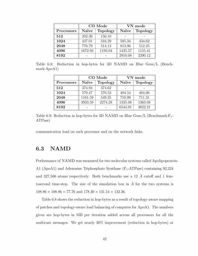
To validate the benefits of topology mapping for LeanCP, we use the perfor-

mance analysis tool in Charm++, called Projections [32]. This tool helps us visu-

alize the average number of hops per entry method and per processor. Figures 6.3

and 6.4 show the average hop-bytes per processor for the naıve and topology map-

ping. Both runs used the WATER 32M 70Ry benchmark and 2,048 processors of

Blue Gene/L in CO mode. As we can see, the average hop-count per processor for

the topology case is 7 compared to 9 for the default case. Also, communication

is much more uniform in the case of topology aware mapping which balances the

40

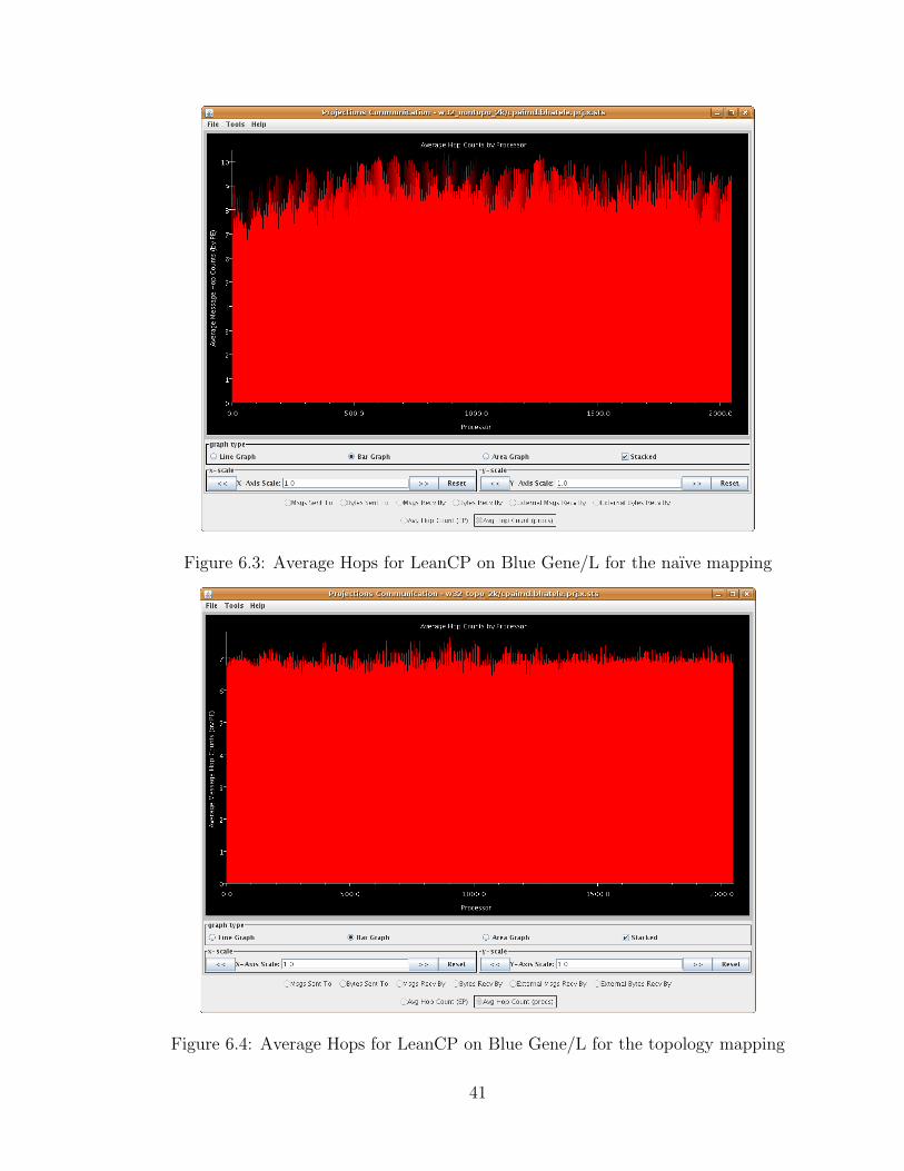
Figure 6.3: Average Hops for LeanCP on Blue Gene/L for the naıve mapping

Figure 6.4: Average Hops for LeanCP on Blue Gene/L for the topology mapping

41

CO Mode VN modeProcessors Naıve Topology Naıve Topology

512 202.39 150.10 - -1024 437.01 316.29 505.34 434.622048 776.79 514.13 813.06 512.254096 1672.93 1193.04 1435.57 1155.418192 - - 2910.08 2290.12

Table 6.8: Reduction in hop-bytes for 3D NAMD on Blue Gene/L (Bench-mark:ApoA1)

CO Mode VN modeProcessors Naıve Topology Naıve Topology

512 374.94 374.62 - -1024 570.47 570.53 484.54 484.062048 1161.59 549.35 710.99 711.314096 3933.59 2274.28 1335.08 1363.088192 - - 6544.91 3822.21

Table 6.9: Reduction in hop-bytes for 3D NAMD on Blue Gene/L (Benchmark:F1-ATPase)

communication load on each processor and on the network links.

6.3 NAMD

Performance of NAMD was measured for two molecular systems called Apolipoprotein-

A1 (ApoA1) and Adenosine Triphosphate Synthase (F1-ATPase) containing 92,224

and 327,506 atoms respectively. Both benchmarks use a 12 A cutoff and 1 fem-

tosecond time-step. The size of the simulation box in A for the two systems is

108.86× 108.86× 77.76 and 178.30× 131.54× 132.36.

Table 6.8 shows the reduction in hop-bytes as a result of topology-aware mapping

of patches and topology-aware load balancing of computes for ApoA1. The numbers

given are hop-bytes in MB per iteration added across all processors for all the

multicast messages. We get nearly 30% improvement (reduction in hop-bytes) at

42

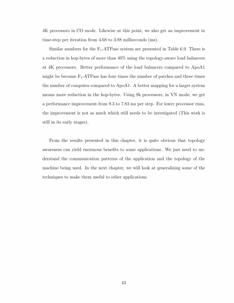
4K processors in CO mode. Likewise at this point, we also get an improvement in

time-step per iteration from 4.68 to 3.88 milliseconds (ms).

Similar numbers for the F1-ATPase system are presented in Table 6.9. There is

a reduction in hop-bytes of more than 40% using the topology-aware load balancers

at 4K processors. Better performance of the load balancers compared to ApoA1

might be because F1-ATPase has four times the number of patches and three times

the number of computes compared to ApoA1. A better mapping for a larger system

means more reduction in the hop-bytes. Using 8k processors, in VN mode, we get

a performance improvement from 9.3 to 7.83 ms per step. For lower processor runs,

the improvement is not as much which still needs to be investigated (This work is

still in its early stages).

From the results presented in this chapter, it is quite obvious that topology

awareness can yield enormous benefits to some applications. We just need to un-

derstand the communication patterns of the application and the topology of the

machine being used. In the next chapter, we will look at generalizing some of the

techniques to make them useful to other applications.

43

7 Future Work and Conclusion

In this thesis, we have focused on specific parallel applications and analyzed the

benefit from topology-aware mapping. The approach has been to understand the

parallel implementation and the communication characteristics of the application.

Based on the communication graph, we have tried to place communicating objects

on nearby processors on a 3D mesh or torus topology. The two different places where

we have done this are: 1. defining a static mapping during start-up as in the case of

3D Jacobi and LeanCP, and 2. modifying the load balancers to take the topology

of machine into account (as in NAMD). So, our effort has been concentrated on a

few specific applications and a 3D mesh or torus topology. We shall now discuss

future efforts to make these ideas more general so that they can be used by other

applications on diverse topologies.

7.1 Generalized Topology Sensitive Mapping

We were quite successful in mapping different chare arrays in LeanCP by con-

sidering their communication dependencies. We wish to extend this idea to do

this for any application with regular communication. Given the communication

dependencies between chare arrays and the topology, the Charm++ RTS should

automatically do an intelligent mapping. This would remove the burden of mapping

from the user and give optimized performance compared to a random mapping.

A more general idea is to successfully do this for any arbitrary communication

graph and topology. This has been proved to be NP-complete by Bokhari [10].

44

Hence the effort would be towards development of heuristics which perform well for

most scenarios. This would useful for problems with regular communication like

Jacobi, Matrix multiplication and FFTs.

7.2 Load Balancers for Section Multicasts

Multicasts in NAMD are a very special case. All patches send the same data to

their multicast targets and each multicast target (compute) receives data from only

two patches. In general, a target can receive messages from any number of multicast

roots.

We plan to build upon the algorithms developed in the NAMD load balancers

to do this for a more general case. We wish to write a load balancer within the

Charm++ load balancing framework which considers generic multicasts and the

topology of the machine. Since it would be within the Charm++ framework,

other applications will also be able to use it. This can be used by applications like

cosmology (ChaNGa [33]) and meshing applications.

7.3 Summary

Work presented in this thesis demonstrates the benefit of topology-awareness in

mapping of objects on to a parallel machine statically or during load balancing. We

first describe the topology interface in Charm++ which facilitates the mapping of

objects onto 3D topologies. As a first example, we take a simple application, 3D

7-point stencil and prove that topology mapping does help in reducing contention

during communication, thereby reducing the time required for the same. The num-

ber of hops travelled by messages is reduced by ten times on the average which gives

us a performance boost of two to seven times in certain cases.

45

The two real applications which benefit from the idea of topology-aware map-

ping are LeanCP and NAMD. LeanCP has regular communication between its

numerous chare arrays and thus provides us with a structured well-defined example

for topology-aware mapping. Since the application is heavily communication bound,

it shows good improvements compared to the naıve mapping. NAMD’s load bal-

ancers on the other hand depend on many factors for optimal performance. Hence,

it becomes difficult to judge the real benefit of topology mapping. Yet NAMD

also shows a reasonable improvement in terms of hop-bytes and some improvement

in performance for higher processor counts. We hope to utilize the insights gained

from the study of these applications to create a generalized automatic framework

for topology-aware mapping. This would benefit many applications in the future.

and performance of the application.

46

References

[1] Tarun Agarwal, Amit Sharma, and Laxmikant V. Kale. Topology-aware taskmapping for reducing communication contention on large parallel machines. InProceedings of IEEE International Parallel and Distributed Processing Sympo-sium 2006, April 2006.

[2] L. V. Kale, B. Ramkumar, A. B. Sinha, and A. Gursoy. The CHARM Par-allel Programming Language and System: Part I – Description of LanguageFeatures. Parallel Programming Laboratory Technical Report #95-02, 1994.

[3] L. V. Kale, B. Ramkumar, A. B. Sinha, and V. A. Saletore. The CHARMParallel Programming Language and System: Part II – The Runtime system.Parallel Programming Laboratory Technical Report #95-03, 1994.

[4] James C. Phillips, Rosemary Braun, Wei Wang, James Gumbart, EmadTajkhorshid, Elizabeth Villa, Christophe Chipot, Robert D. Skeel, LaxmikantKale, and Klaus Schulten. Scalable molecular dynamics with NAMD. Journalof Computational Chemistry, 26(16):1781–1802, 2005.

[5] James C. Phillips, Gengbin Zheng, Sameer Kumar, and Laxmikant V. Kale.NAMD: Biomolecular simulation on thousands of processors. In Proceedingsof the 2002 ACM/IEEE conference on Supercomputing, pages 1–18, Baltimore,MD, September 2002.

[6] Ramkumar V. Vadali, Yan Shi, Sameer Kumar, L. V. Kale, Mark E. Tuck-erman, and Glenn J. Martyna. Scalable fine-grained parallelization of plane-wave-based ab initio molecular dynamics for large supercomputers. Journal ofComptational Chemistry, 25(16):2006–2022, Oct. 2004.

[7] Eric Bohm, Glenn J. Martyna, Abhinav Bhatele, Sameer Kumar, Laxmikant V.Kale, John A. Gunnels, and Mark E. Tuckerman. Fine Grained Parallelizationof the Car-Parrinello ab initio MD Method on Blue Gene/L. IBM Journalof Research and Development: Applications of Massively Parallel Systems (toappear), 52(1/2), 2007.

[8] M.Blumrich, D.Chen, P.Coteus, A.Gara, M.Giampapa, P.Heidelberger,S.Singh, B.Steinmacher-Burow, T.Takken, and P.Vranas. Design and analy-sis of the blue gene/l torus interconnection network. IBM Research Report,December 2003.

47

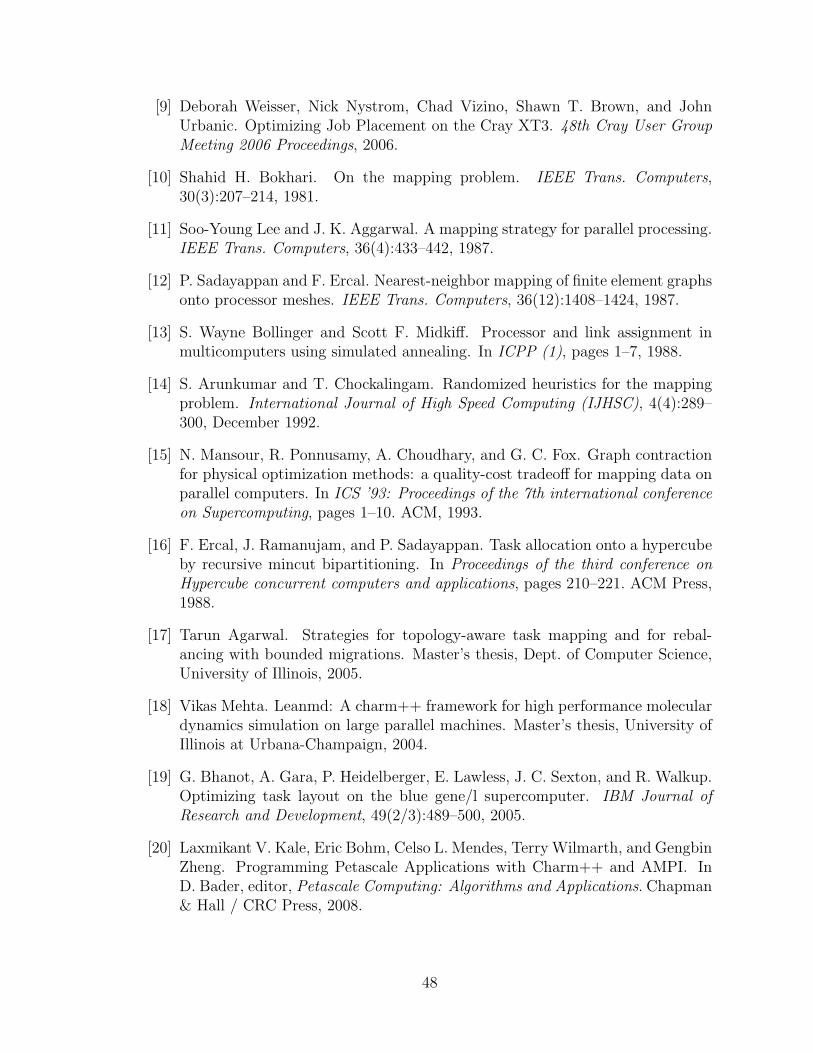
[9] Deborah Weisser, Nick Nystrom, Chad Vizino, Shawn T. Brown, and JohnUrbanic. Optimizing Job Placement on the Cray XT3. 48th Cray User GroupMeeting 2006 Proceedings, 2006.

[10] Shahid H. Bokhari. On the mapping problem. IEEE Trans. Computers,30(3):207–214, 1981.

[11] Soo-Young Lee and J. K. Aggarwal. A mapping strategy for parallel processing.IEEE Trans. Computers, 36(4):433–442, 1987.

[12] P. Sadayappan and F. Ercal. Nearest-neighbor mapping of finite element graphsonto processor meshes. IEEE Trans. Computers, 36(12):1408–1424, 1987.

[13] S. Wayne Bollinger and Scott F. Midkiff. Processor and link assignment inmulticomputers using simulated annealing. In ICPP (1), pages 1–7, 1988.

[14] S. Arunkumar and T. Chockalingam. Randomized heuristics for the mappingproblem. International Journal of High Speed Computing (IJHSC), 4(4):289–300, December 1992.

[15] N. Mansour, R. Ponnusamy, A. Choudhary, and G. C. Fox. Graph contractionfor physical optimization methods: a quality-cost tradeoff for mapping data onparallel computers. In ICS ’93: Proceedings of the 7th international conferenceon Supercomputing, pages 1–10. ACM, 1993.

[16] F. Ercal, J. Ramanujam, and P. Sadayappan. Task allocation onto a hypercubeby recursive mincut bipartitioning. In Proceedings of the third conference onHypercube concurrent computers and applications, pages 210–221. ACM Press,1988.

[17] Tarun Agarwal. Strategies for topology-aware task mapping and for rebal-ancing with bounded migrations. Master’s thesis, Dept. of Computer Science,University of Illinois, 2005.

[18] Vikas Mehta. Leanmd: A charm++ framework for high performance moleculardynamics simulation on large parallel machines. Master’s thesis, University ofIllinois at Urbana-Champaign, 2004.

[19] G. Bhanot, A. Gara, P. Heidelberger, E. Lawless, J. C. Sexton, and R. Walkup.Optimizing task layout on the blue gene/l supercomputer. IBM Journal ofResearch and Development, 49(2/3):489–500, 2005.

[20] Laxmikant V. Kale, Eric Bohm, Celso L. Mendes, Terry Wilmarth, and GengbinZheng. Programming Petascale Applications with Charm++ and AMPI. InD. Bader, editor, Petascale Computing: Algorithms and Applications. Chapman& Hall / CRC Press, 2008.

48

[21] L. V. Kale and Sanjeev Krishnan. Charm++: Parallel Programming withMessage-Driven Objects. In Gregory V. Wilson and Paul Lu, editors, ParallelProgramming using C++, pages 175–213. MIT Press, 1996.

[22] Sameer Kumar, Chao Huang, Gheorghe Almasi, and Laxmikant V. Kale.Achieving strong scaling with NAMD on Blue Gene/L. In Proceedings of IEEEInternational Parallel and Distributed Processing Symposium 2006, April 2006.

[23] Sameer Kumar, Chao Huang, Gengbin Zheng, Eric Bohm, Abhinav Bhatele,James C. Phillips, Hao Yu, and Laxmikant V. Kale. Scalable Molecular Dynam-ics with NAMD on Blue Gene/L. IBM Journal of Research and Development:Applications of Massively Parallel Systems (to appear), 52(1/2), 2007.

[24] R. Car and M. Parrinello. Unified approach for molecular dynamics and density-functional theory. Phys. Rev. Lett., 55:2471–2474, (1985).

[25] G. Galli and M. Parrinello. Computer Simulation in Materials Science, 3:283,(1991).

[26] M.C. Payne, M. Teter, D.C. Allan, T.A. Aria, and J.D. Joannopolous. Itera-tive minimization techniques for ab initio total energy calculations : moleculardynamics and conjugate gradients. Rev. Mod. Phys., 64:1045, (1992).

[27] M. E. Tuckerman. Ab initio molecular dynamics: Basic concepts, current trendsand novel applications. J. Phys. Condensed Matter, 14:R1297, 2002.

[28] H.S. Lee, M.E. Tuckerman, and G.J. Martyna. Efficient evaluation of nonlo-cal pseudopotentials via euler exponential spline interpolation. Chem. Phys.Chem., 6:1827, (2005).

[29] Abhinav Bhatele, Sameer Kumar, Chao Mei, James C. Phillips, Gengbin Zheng,and Laxmikant V. Kale. NAMD: A Portable and Highly Scalable Program forBiomolecular Simulations. 2007.

[30] Klaus Schulten, James C. Phillips, Laxmikant V. Kale, and Abhinav Bhatele.Biomolecular modeling in the era of petascale computing. In D. Bader, editor,Petascale Computing: Algorithms and Applications, pages 165–181. Chapman& Hall / CRC Press, 2008.

[31] Laxmikant Kale, Robert Skeel, Milind Bhandarkar, Robert Brunner, AttilaGursoy, Neal Krawetz, James Phillips, Aritomo Shinozaki, Krishnan Varadara-jan, and Klaus Schulten. NAMD2: Greater scalability for parallel moleculardynamics. Journal of Computational Physics, 151:283–312, 1999.

[32] Laxmikant V. Kale, Gengbin Zheng, Chee Wai Lee, and Sameer Kumar. Scal-ing applications to massively parallel machines using projections performanceanalysis tool. In Future Generation Computer Systems Special Issue on: Large-Scale System Performance Modeling and Analysis, volume 22, pages 347–358,February 2006.

49

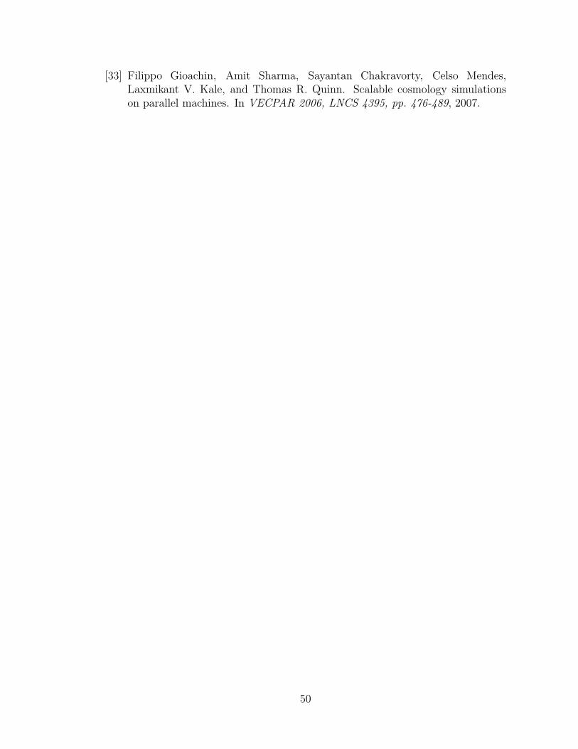
[33] Filippo Gioachin, Amit Sharma, Sayantan Chakravorty, Celso Mendes,Laxmikant V. Kale, and Thomas R. Quinn. Scalable cosmology simulationson parallel machines. In VECPAR 2006, LNCS 4395, pp. 476-489, 2007.

50

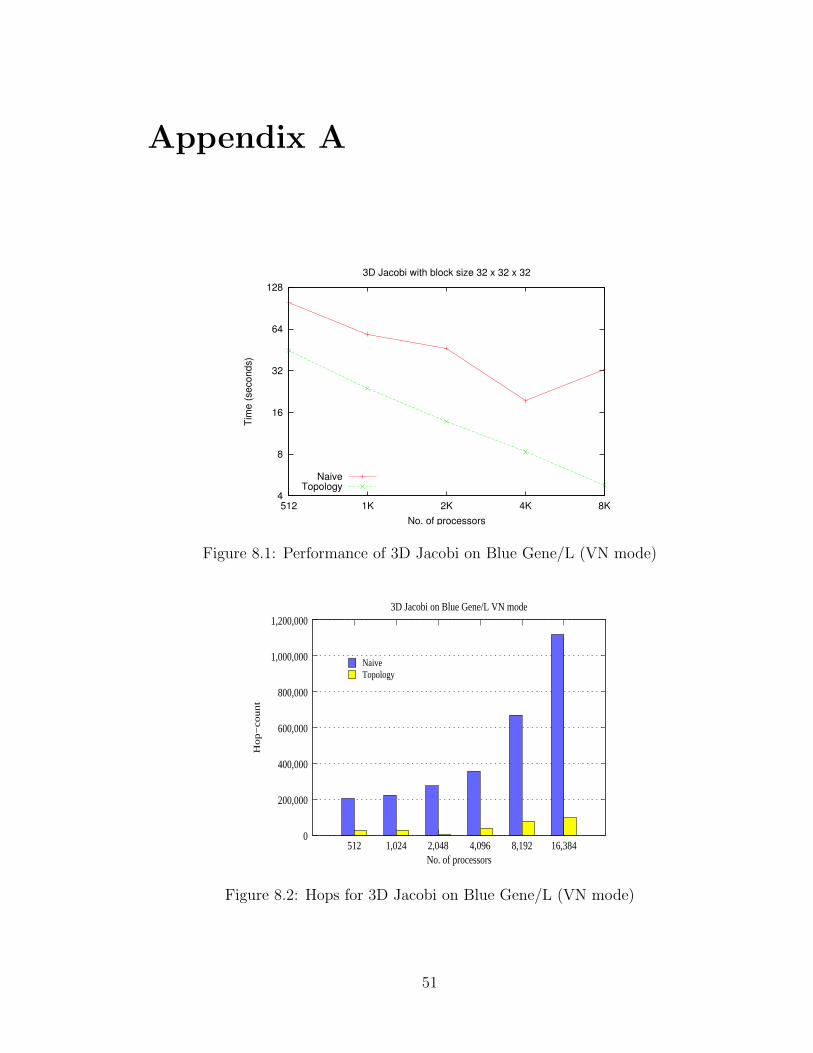
Appendix A

4

8

16

32

64

128

512 1K 2K 4K 8K

Tim

e (s

econ

ds)

No. of processors

3D Jacobi with block size 32 x 32 x 32

NaiveTopology

Figure 8.1: Performance of 3D Jacobi on Blue Gene/L (VN mode)

NaiveTopology

0

200,000

400,000

600,000

800,000

1,000,000

1,200,000

512 1,024 2,048 4,096 8,192 16,384

Ho

p−

co

un

t

No. of processors

3D Jacobi on Blue Gene/L VN mode

Figure 8.2: Hops for 3D Jacobi on Blue Gene/L (VN mode)

51

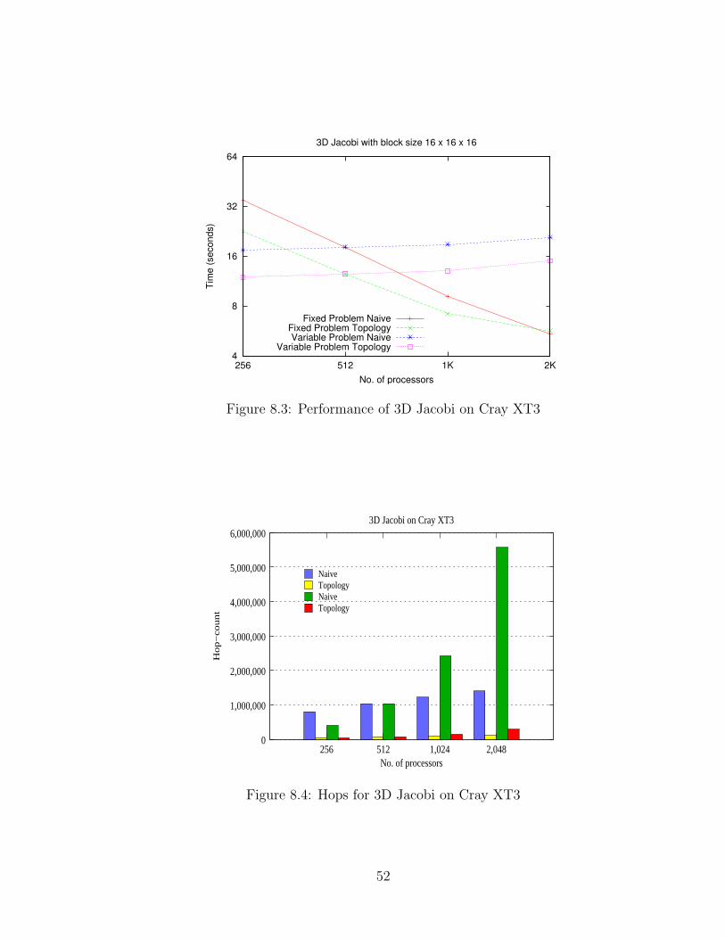
4

8

16

32

64

256 512 1K 2K

Tim

e (s

econ

ds)

No. of processors

3D Jacobi with block size 16 x 16 x 16

Fixed Problem NaiveFixed Problem TopologyVariable Problem Naive

Variable Problem Topology

Figure 8.3: Performance of 3D Jacobi on Cray XT3

NaiveTopologyNaiveTopology

0

1,000,000

2,000,000

3,000,000

4,000,000

5,000,000

6,000,000

256 512 1,024 2,048

Ho

p−

co

un

t

No. of processors

3D Jacobi on Cray XT3

Figure 8.4: Hops for 3D Jacobi on Cray XT3

52

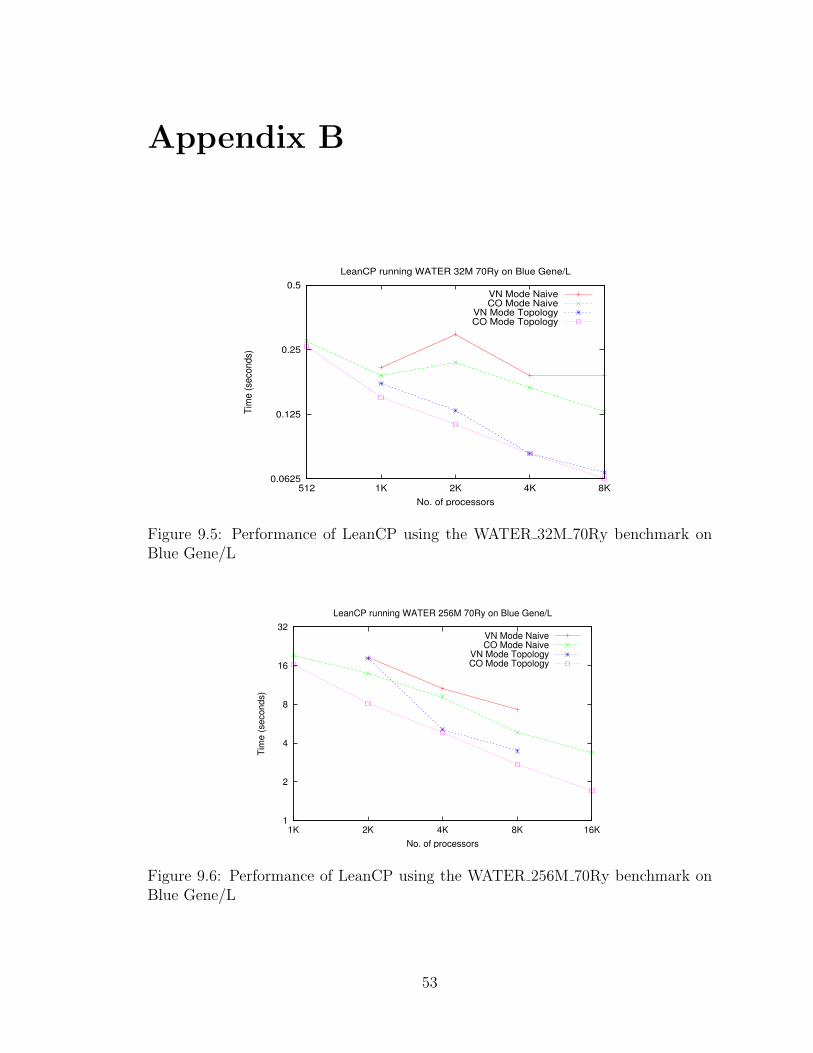
Appendix B

0.0625

0.125

0.25

0.5

512 1K 2K 4K 8K

Tim

e (s

econ

ds)

No. of processors

LeanCP running WATER 32M 70Ry on Blue Gene/L

VN Mode NaiveCO Mode Naive

VN Mode TopologyCO Mode Topology

Figure 9.5: Performance of LeanCP using the WATER 32M 70Ry benchmark onBlue Gene/L

1

2

4

8

16

32

1K 2K 4K 8K 16K

Tim

e (s

econ

ds)

No. of processors

LeanCP running WATER 256M 70Ry on Blue Gene/L

VN Mode NaiveCO Mode Naive

VN Mode TopologyCO Mode Topology

Figure 9.6: Performance of LeanCP using the WATER 256M 70Ry benchmark onBlue Gene/L

53

Appendix C

The Topology API in Charm++ provides the user application with a lot of useful

functions which facilitate the implementation of mapping algorithms. It should be

noted that these functions are only applicable for 3D mesh and torus topologies:

void rankToCoordinates(int pe, int &x, int &y, int &z) This function re-

turns the physical co-ordinates on the machine for a given processor rank or

ID (assigned by the system).

int coordinatesToRank(int x, int y, int z) This function returns the sys-

tem assigned processor rank for given physical co-ordinates (x, y, z) on the

machine.

int getHopsBetweenRanks(int pe1, int pe2) This returns the number of hops

between two processors.

void sortRanksByHops(int pe, int *pes, int *idx, int n) Given a list of pro-

cessors, this function sorts the list by their distance in hops from a given

processor.

int pickClosestRank(int mype, int *pes, int n) This function picks the clos-

est processor to a given processor from a given list.

int areNeighbors(int pe1, int pe2, int pe3, int distance) This function

determines if the sum of the distance in hops between three processors is less

than a certain distance.

54

These functions are used in LeanCP and NAMD extensively to simplify the

mapping algorithms. For example, to sort a list of processors by their distance from

their centroid, we can do the following:

void sortByCentroid(int *list, int npes) {

int pe, x, y, z, x1, y1, z1;

int idx[npes];

for(int i=0; i<npes; i++) {

rankToCoordinates(list[i], x1, y1, z1);

x += x1;

y += y1;

z += z1;

}

x = x/npes;

y = y/npes;

z = z/npes;

pe = coordinatesToRank(x, y, z);

sortRanksByHops(pe, list, idx, npes);

}

55

Vita

Office Address: Residential Address:

Thomas M. Siebel Center for Comp. Sc. 505, E White St, Apt. #06

201, N. Goodwin Avenue, Champaign, IL 61820

Urbana, IL 61801 Ph: +1-217-417-7579

http://charm.cs.uiuc.edu/~bhatele E-mail: bhatele2@uiuc.edu

Abhinav Bhatele

Educational Qualifications

Doctor of Philosophy in Computer Science 2005 – Present

University of Illinois at Urbana Champaign CGPA: 3.89/4.0

Bachelor of Technology in Computer Science and Engineering 2001-2005

Indian Institute of Technology, Kanpur CPI: 9.1/10.0

Research Experience

Graduate Research Assistant, Parallel Programming Laboratory, UIUC

2005-Present

Working with Prof. Laxmikant V. Kale in the Parallel Programming Group at UIUC

since August 2005.

• I work on molecular dynamics applications called NAMD and LeanCP written

56

in Charm++. My work is related to topology sensitive mapping and load-

balancing.

• Working on BigSim, a Parallel Discrete Event Simulator developed at PPL.

Summer Intern, IBM T J Watson Research Center, NY, USA May-July

2007

Worked with Dr. Sameer Kumar in the Blue Gene Software Group

• Devised topology sensitive load balancing algorithms to be applied to Charm++

programs in general and NAMD in particular.

Summer Intern, IBM T J Watson Research Center, NY, USA May-July

2006

Worked with Dr. Guojing Cong at the Advanced Computing Technology Center

• Developed a tool for automatic and detailed profiling of programs at finer

levels like functions and individual statements.

Summer Intern, INRIA Labs, Nancy, France May-July 2004

Worked with Prof. Dominique Mery and Stephan Merz in the MOSEL group

• Developed a GUI for TLC and Xprove: TLC is a model checker and Xprove

is a theorem prover being developed at INRIA Labs.

Summer Intern, IIT Kanpur, India May-July 2003

Worked with Prof. Shashank K. Mehta at IIT Kanpur

• Studied a Picoblaze microprocessor design in VHDL (developed by Xilinx)

and implemented and tested it using Verilog.

57

Recent Publications

1. Abhinav Bhatele, Sameer Kumar, Chao Mei, James C. Phillips, Gengbin

Zheng, Laxmikant V. Kale, NAMD: A Portable and Highly Scalable Program

for Biomolecular Simulations, PPL Technical Report, 2007

2. Abhinav Bhatele, Guojing Cong, A Selective Profiling Tool: Towards Auto-

matic Performance Tuning, In Proceedings of SMTPS 07, IPDPS, 2007

3. Abhinav Bhatele, Shubham Satyarth, Sanjeev K. Aggarwal, Compiler Algo-

rithm Language (CAL): An Interpreter and Compiler, In Proceedings of ACST,

2007

4. Klaus Schulten, James C. Phillips, Laxmikant V. Kale, Abhinav Bhatele,

Biomolecular modeling in the era of petascale computing, In Petascale Com-

puting: Algorithms and Applications, pp. 165-181, D. Bader, Ed., Chapman

& Hall / CRC Press, New York, 2007

5. Eric Bohm, Abhinav Bhatele, Laxmikant V. Kale, Mark E. Tuckerman, Sameer

Kumar, John A. Gunnels, Glenn Martyna, Fine grained parallelization of the

Car-Parrinello ab initio MD method on Blue Gene/L, In IBM J. Res. Dev.,

Volume 52, No. 1/2, 2007

6. Sameer Kumar, Chao Huang, Gengbin Zheng, Eric Bohm, Abhinav Bhatele,

Jim Phillips, Gheorghe Almasi, Hao Yu, Laxmikant V. Kale, Achieving Strong

Scaling with NAMD on Blue Gene/L, In IBM J. Res. Dev., Volume 52, No.

1/2, 2007

Relevant Courses

Graduate – Advanced Computer Architecture (CS533), Formal Methods of Com-

putation (CS475), Parallel Programming Methods (CS498lvk), Programming Lan-

guages and Compilers (CS421), Advanced Topics in Compiler Construction (CS526),

58

Social Computing (CS598kgk), Improving your Research Skills (CS598lrs)

Undergraduate – Advanced Compiler Optimizations (CS738), Computer Archi-

tecture (CS422), Compilers (CS335), Computer Networks (CS425), Operating Sys-

tems (CS330), Algorithms II (CS345), Theory of Computation (CS340), Data Struc-

tures and Algorithms (CS210), Discrete Mathematics (CS201)

Programming Skills

Languages: Charm++, C, C++, JAVA, Verilog, VHDL, Scheme, ML, Ocaml

Platforms: Most flavors of Windows and Linux

Tools: Lex, Yacc, LaTeX, Make, Perl

Graduate Projects

Optimizing LeanMD on Blue Gene/L – Topology mapping for this basic molec-

ular dynamics code on the Blue Gene machine

Review of Barnes-Hut Implementation in Several Parallel Programming

Models – Survey of which parallel programming are a good fit for the Barnes Hut

problem

SocViz: Visualization of Facebook Data – A HCI Study and development of

a visualization tool for social networking data

Undergraduate Projects

Compiler Algorithm Language (CAL): An Interpreter and Compiler – De-

signed a new language to help compiler writers express their algorithms in a more

natural way.

Picoblaze 8-bit Microprocessor – Studied this multiprocessors design and im-

plemented and tested it in Verilog HDL.

59

Performance of TCP over Multiple Wireless Interface – Solved the problem

of Loss Isolation in Multiple Wireless Interfaces by using TCP-in-TCP mechanism.

LaTeX Compiler – (A reduced subset of it) was developed as a part of the com-

piler course CS335.

Extended Nachos Project – Implemented a subset of the OS as a part of the

operating systems course CS330.

Awards and Achievements

• Instructor for a class of 40 students for the “Data Structures and Algorithms”

course

• Nominated among the six best B. Tech. projects (2005) in the Computer

Science department

• Awarded the Student Benefit Fund Scholarship for excellent performance in

academics in 2002

• Awarded the Academic Excellence Award at IIT Kanpur for the year 2001-

2002

• Received a certificate of merit in the Indian National Physics Olympiad 2001

• Received a certificate of merit in the Indian National Chemistry Olympiad

2001

• Adjudged the best student and awarded the Gold Medal in 2000 in high school

for excellent academic performance

• Received the SAIL Scholarship in high school in 1999 for Grade 10th perfor-

mance.

60

References

Prof. Laxmikant V. Kale (kale@cs.uiuc.edu), Professor, Dept. Of Computer Sci-

ence, UIUC

Dr. Glenn J. Martyna (martyna@us.ibm.com), Researcher, IBM T J Watson Re-

search, NY

Dr. Sameer Kumar (sameerk@us.ibm.com), Researcher, IBM T J Watson Research,

NY

Dr. Guojing Cong (gcong@us.ibm.com), Researcher, IBM T J Watson Research,

NY

Prof. Sanjeev K. Aggarwal (ska@iitk.ac.in), Professor, Dept. Of Computer Science,

IITK

61