NETWORK CENTRIC TRAFFIC ANALYSIS

By

JIEYAN FAN

A DISSERTATION PRESENTED TO THE GRADUATE SCHOOLOF THE UNIVERSITY OF FLORIDA IN PARTIAL FULFILLMENT

OF THE REQUIREMENTS FOR THE DEGREE OFDOCTOR OF PHILOSOPHY

UNIVERSITY OF FLORIDA

2007

1

c© 2007 Jieyan Fan

2

To those who sparked my interest in science, opening for me the door to discovering

nature and letting me walk through it in my own way.

3

ACKNOWLEDGMENTS

First of all, thank my advisor Professor Dapeng Wu for his great inspiration, excellent

guidance, deep thoughts, and friendship. I also thank my supervisory committee members,

Professors Shigang Chen, Liuqing Yang, and Tao Li, for their interest in my work.

I also express my appreciation to all of the faculty, staff, and my fellow students

in the Department of Electrical and Computer Engineering. In particular, I extend my

thanks to Dr. Kejie Lu for his helpful discussions.

4

TABLE OF CONTENTS

page

ACKNOWLEDGMENTS . . . . . . . . . . . . . . . . . . . . . . . . . . . . . . . . . 4

LIST OF TABLES . . . . . . . . . . . . . . . . . . . . . . . . . . . . . . . . . . . . . 8

LIST OF FIGURES . . . . . . . . . . . . . . . . . . . . . . . . . . . . . . . . . . . . 9

ABSTRACT . . . . . . . . . . . . . . . . . . . . . . . . . . . . . . . . . . . . . . . . 12

CHAPTER

1 INTRODUCTION . . . . . . . . . . . . . . . . . . . . . . . . . . . . . . . . . . 14

1.1 Introduction to Network Anomaly Detection . . . . . . . . . . . . . . . . . 141.2 Introduction to Network Centric Traffic Classification . . . . . . . . . . . . 16

2 NETWORK ANOMALY DETECTION FRAMEWORK . . . . . . . . . . . . . 18

2.1 Introduction . . . . . . . . . . . . . . . . . . . . . . . . . . . . . . . . . . . 182.2 Edge-Router Based Network Anomaly Detection Framework . . . . . . . . 18

2.2.1 Traffic Monitor . . . . . . . . . . . . . . . . . . . . . . . . . . . . . 202.2.2 Local Analyzer . . . . . . . . . . . . . . . . . . . . . . . . . . . . . 202.2.3 Global Analyzer . . . . . . . . . . . . . . . . . . . . . . . . . . . . . 21

2.3 Summary . . . . . . . . . . . . . . . . . . . . . . . . . . . . . . . . . . . . 22

3 FEATURES FOR NETWORK ANOMALY DETECTION . . . . . . . . . . . . 23

3.1 Introduction . . . . . . . . . . . . . . . . . . . . . . . . . . . . . . . . . . . 233.2 Hierarchical Feature Extraction Architecture . . . . . . . . . . . . . . . . . 24

3.2.1 Three-Level Design . . . . . . . . . . . . . . . . . . . . . . . . . . . 243.2.2 Feature Extraction in a Traffic Monitor . . . . . . . . . . . . . . . . 263.2.3 Feature Extraction in a Local Analyzer or a Global Analyzer . . . . 27

3.3 Two-Way Matching Features . . . . . . . . . . . . . . . . . . . . . . . . . . 273.3.1 Motivation . . . . . . . . . . . . . . . . . . . . . . . . . . . . . . . . 273.3.2 Definition of Two-Way Matching Features . . . . . . . . . . . . . . 30

3.4 Basic Algorithms . . . . . . . . . . . . . . . . . . . . . . . . . . . . . . . . 323.4.1 Hash Table Algorithm . . . . . . . . . . . . . . . . . . . . . . . . . 323.4.2 Bloom Filter . . . . . . . . . . . . . . . . . . . . . . . . . . . . . . . 33

3.5 Bloom Filter Array (BFA) . . . . . . . . . . . . . . . . . . . . . . . . . . . 353.5.1 Data Structure . . . . . . . . . . . . . . . . . . . . . . . . . . . . . 353.5.2 Algorithm . . . . . . . . . . . . . . . . . . . . . . . . . . . . . . . . 363.5.3 Round Robin Sliding Window . . . . . . . . . . . . . . . . . . . . . 383.5.4 Random-Keyed Hash Functions . . . . . . . . . . . . . . . . . . . . 39

3.6 Complexity Analysis . . . . . . . . . . . . . . . . . . . . . . . . . . . . . . 403.6.1 Space/Time Trade-off . . . . . . . . . . . . . . . . . . . . . . . . . . 413.6.2 Optimal Parameter Setting for Bloom Filter Array . . . . . . . . . . 50

5

3.7 Simulation Results . . . . . . . . . . . . . . . . . . . . . . . . . . . . . . . 513.7.1 The BFA Algorithm vs. the Hash Table Algorithm . . . . . . . . . . 513.7.2 Experiment on Feature Extraction System . . . . . . . . . . . . . . 55

3.8 Summary . . . . . . . . . . . . . . . . . . . . . . . . . . . . . . . . . . . . 57

4 MACHINE LEARNING ALGORITHM FOR NETWORK ANOMALYDETECTION . . . . . . . . . . . . . . . . . . . . . . . . . . . . . . . . . . . . . 59

4.1 Introduction . . . . . . . . . . . . . . . . . . . . . . . . . . . . . . . . . . . 594.1.1 Receiver Operating Characteristics Curve . . . . . . . . . . . . . . . 594.1.2 Threshold-Based Algorithm . . . . . . . . . . . . . . . . . . . . . . 604.1.3 Change-Point Algorithm . . . . . . . . . . . . . . . . . . . . . . . . 604.1.4 Bayesian Decision Theory . . . . . . . . . . . . . . . . . . . . . . . . 62

4.2 Bayesian Model for Network Anomaly Detection . . . . . . . . . . . . . . . 644.2.1 Bayesian Model for Traffic Monitors and Local Analyzers . . . . . . 644.2.2 Bayesian Model for Global Analyzers . . . . . . . . . . . . . . . . . 664.2.3 Hidden Markov Tree (HMT) Model for Global Analyzer . . . . . . . 68

4.3 Estimation of HMT Parameters . . . . . . . . . . . . . . . . . . . . . . . . 724.3.1 Likelihood Estimation . . . . . . . . . . . . . . . . . . . . . . . . . . 724.3.2 Transition Probability Estimation . . . . . . . . . . . . . . . . . . . 76

4.4 Network Anomaly Detection Using HMT . . . . . . . . . . . . . . . . . . . 814.5 Simulation Results . . . . . . . . . . . . . . . . . . . . . . . . . . . . . . . 84

4.5.1 Experiment Setting . . . . . . . . . . . . . . . . . . . . . . . . . . . 844.5.2 Performance Comparison . . . . . . . . . . . . . . . . . . . . . . . . 864.5.3 Discussion . . . . . . . . . . . . . . . . . . . . . . . . . . . . . . . . 88

4.6 Summary . . . . . . . . . . . . . . . . . . . . . . . . . . . . . . . . . . . . 89

5 NETWORK CENTRIC TRAFFIC CLASSIFICATION: AN OVERVIEW . . . . 90

5.1 Introduction . . . . . . . . . . . . . . . . . . . . . . . . . . . . . . . . . . . 905.2 Related Work . . . . . . . . . . . . . . . . . . . . . . . . . . . . . . . . . . 945.3 Intuitions Behind a Proper Detection of Voice and Video Streams . . . . . 95

5.3.1 Packet Inter-Arrival Time and Packet Size in Time Domain . . . . . 975.3.2 Packet Inter-Arrival Time in Frequency Domain . . . . . . . . . . . 995.3.3 Packet Size in Frequency Domain . . . . . . . . . . . . . . . . . . . 995.3.4 Combining Packet Inter-Arrival Time and Packet Size in Frequency

Domain . . . . . . . . . . . . . . . . . . . . . . . . . . . . . . . . . . 1005.4 Summary . . . . . . . . . . . . . . . . . . . . . . . . . . . . . . . . . . . . 102

6 NETWORK CENTRIC TRAFFIC CLASSIFICATION SYSTEM . . . . . . . . 104

6.1 System Architecture . . . . . . . . . . . . . . . . . . . . . . . . . . . . . . 1046.1.1 Flow Summary Generator (FSG) . . . . . . . . . . . . . . . . . . . 1056.1.2 Feature Extactor (FE) and Voice/Video Subspace Generator (SG) . 1056.1.3 Voice/Video CLassifer (CL) . . . . . . . . . . . . . . . . . . . . . . 106

6.2 Feature Extractor (FE) Module via Power Spectral Density (PSD) . . . . . 1076.2.1 Modeling the network flow as a stochastic digital process . . . . . . 107

6

6.2.2 Power Spectral Density (PSD) Computation . . . . . . . . . . . . . 1086.3 Subspace Decomposition and Bases Identification on PSD Features . . . . 115

6.3.1 Subspace Decomposition Based on Minimum Coding Length . . . . 1176.3.2 Subspace Bases Identification . . . . . . . . . . . . . . . . . . . . . . 120

6.4 Voice/Video Classifier . . . . . . . . . . . . . . . . . . . . . . . . . . . . . 1216.5 Experiment Results . . . . . . . . . . . . . . . . . . . . . . . . . . . . . . . 123

6.5.1 Experiment Settings . . . . . . . . . . . . . . . . . . . . . . . . . . . 1236.5.2 Skype Flow Classification . . . . . . . . . . . . . . . . . . . . . . . . 1246.5.3 General Flow Classification . . . . . . . . . . . . . . . . . . . . . . . 1246.5.4 Discussion . . . . . . . . . . . . . . . . . . . . . . . . . . . . . . . . 125

6.6 Summary . . . . . . . . . . . . . . . . . . . . . . . . . . . . . . . . . . . . 128

7 CONCLUSION AND FUTURE WORK . . . . . . . . . . . . . . . . . . . . . . 129

7.1 Summary of Network Centric Anomaly Detection . . . . . . . . . . . . . . 1297.2 Summary of Network Centric Traffic Classification . . . . . . . . . . . . . . 131

APPENDIX

A PROOFS . . . . . . . . . . . . . . . . . . . . . . . . . . . . . . . . . . . . . . . 133

A.1 Equation (4–31) . . . . . . . . . . . . . . . . . . . . . . . . . . . . . . . . . 133A.2 Equation (4–32) . . . . . . . . . . . . . . . . . . . . . . . . . . . . . . . . . 133A.3 Equation (4–33) . . . . . . . . . . . . . . . . . . . . . . . . . . . . . . . . . 134A.4 Equation (4–34) . . . . . . . . . . . . . . . . . . . . . . . . . . . . . . . . . 134

REFERENCES . . . . . . . . . . . . . . . . . . . . . . . . . . . . . . . . . . . . . . . 135

BIOGRAPHICAL SKETCH . . . . . . . . . . . . . . . . . . . . . . . . . . . . . . . . 140

7

LIST OF TABLES

Table page

3-1 Notations for two-way matching features . . . . . . . . . . . . . . . . . . . . . . 31

3-2 Notations for complexity analysis . . . . . . . . . . . . . . . . . . . . . . . . . . 41

3-3 Space/time complexity for hash table, Bloom filter, and BFA . . . . . . . . . . . 47

4-1 Parameters used in CUSUM . . . . . . . . . . . . . . . . . . . . . . . . . . . . . 60

4-2 Notations for hidden markov tree model . . . . . . . . . . . . . . . . . . . . . . 70

4-3 Parameter setting of feature extraction for network anomaly detection . . . . . . 86

4-4 Performance of different schemes. . . . . . . . . . . . . . . . . . . . . . . . . . . 86

5-1 Commonly used speech codec and their specifications . . . . . . . . . . . . . . . 96

6-1 Typical PD and PFA values. . . . . . . . . . . . . . . . . . . . . . . . . . . . . . 126

8

LIST OF FIGURES

Figure page

2-1 An ISP network architecture. . . . . . . . . . . . . . . . . . . . . . . . . . . . . 19

2-2 Network anomaly detection framework. . . . . . . . . . . . . . . . . . . . . . . . 19

2-3 Responsibilities of and interactions among the traffic monitor, local analyzer,and global analyzer. . . . . . . . . . . . . . . . . . . . . . . . . . . . . . . . . . 20

2-4 Example of asymmetric traffic whose feature extraction is done by the globalanalyzer. . . . . . . . . . . . . . . . . . . . . . . . . . . . . . . . . . . . . . . . . 21

3-1 Hierarchical structure for feature extraction. . . . . . . . . . . . . . . . . . . . . 24

3-2 Network in normal condition. . . . . . . . . . . . . . . . . . . . . . . . . . . . . 28

3-3 Source-address-spoofed packets. . . . . . . . . . . . . . . . . . . . . . . . . . . . 29

3-4 Reroute. . . . . . . . . . . . . . . . . . . . . . . . . . . . . . . . . . . . . . . . . 29

3-5 Hash Table Algorithm . . . . . . . . . . . . . . . . . . . . . . . . . . . . . . . . 33

3-6 Bloom Filter Operations . . . . . . . . . . . . . . . . . . . . . . . . . . . . . . . 34

3-7 Scenarios of the problems caused by Bloom filter. (a) Boundary problem. (b)An outbound packet arrives before its matched inbound packet with t2 − t1 < Γ. 34

3-8 Bloom Filter Array Algorithm . . . . . . . . . . . . . . . . . . . . . . . . . . . . 37

3-9 Bloom Filter Array Algorithm using sliding window . . . . . . . . . . . . . . . . 38

3-10 Space/time trade-off for the hash table, BFA with η = 0.1%, and BFA with η =1% . . . . . . . . . . . . . . . . . . . . . . . . . . . . . . . . . . . . . . . . . . . 48

3-11 Relation among space complexity, time complexity, and collision probability.(a) M∗

a vs. η. (b) E[Ta]∗ vs. η. . . . . . . . . . . . . . . . . . . . . . . . . . . . 50

3-12 Space complexity vs. collision probability for fixed time complexity. . . . . . . . 52

3-13 Memory size (in bits) vs. average processing time per query (in µs) . . . . . . . 53

3-14 Average processing time per query (in µs) vs. average number of hash functioncalculations per query. . . . . . . . . . . . . . . . . . . . . . . . . . . . . . . . . 54

3-15 Comparison of numerical and simulation results. (a) Hash table algorithm. (b)BFA algorithm with η=1%. . . . . . . . . . . . . . . . . . . . . . . . . . . . . . 55

3-16 Feature data: (a) Number of SYN packets (link 1), (b) Number of unmatchedSYN packets (link 1), (c) Number of SYN packets (link 2), and (d) Number ofunmatched SYN packets (link 2). . . . . . . . . . . . . . . . . . . . . . . . . . . 58

9

4-1 Generative process in graphical representation, in which the traffic state generatesthe stochastic process of traffic. . . . . . . . . . . . . . . . . . . . . . . . . . . . 64

4-2 Extended generative model including traffic feature vectors: (a) original modeland (b) simplified model. . . . . . . . . . . . . . . . . . . . . . . . . . . . . . . 65

4-3 Generative independent model that describes dependencies among traffic statesand traffic feature vectors. . . . . . . . . . . . . . . . . . . . . . . . . . . . . . . 66

4-4 Generative dependent model that describes dependencies among edge routers. . 67

4-5 Hidden Markov tree model. For an node i, ρ(i) denotes its parent node and ν(i)denotes the set of its children nodes. . . . . . . . . . . . . . . . . . . . . . . . . 69

4-6 Probability density function of the univariate Gaussian distribution N (x; 0, 1). . 73

4-7 Histogram of the two-way matching features measured at a real network duringnetwork anomalies. . . . . . . . . . . . . . . . . . . . . . . . . . . . . . . . . . . 73

4-8 The EM algorithm for estimating p(φi|Ωi = u), i ∈ Ξ, u ∈ 0, 1. . . . . . . . . . 75

4-9 Iteratively estimate transition probabilities. . . . . . . . . . . . . . . . . . . . . 77

4-10 Belief propagation algorithm. . . . . . . . . . . . . . . . . . . . . . . . . . . . . 78

4-11 Viterbi algorithm for HMT decoding. . . . . . . . . . . . . . . . . . . . . . . . . 82

4-12 Experiment Network . . . . . . . . . . . . . . . . . . . . . . . . . . . . . . . . . 85

4-13 Performance of threshold-based and machine learning algorithms with differentfeature data . . . . . . . . . . . . . . . . . . . . . . . . . . . . . . . . . . . . . . 87

4-14 Performance of four detection algorithms . . . . . . . . . . . . . . . . . . . . . . 88

5-1 Average packet size versus inter-arrival variability metric for 5 applications: voice,video, file transfer, mix of file transfer with voice and video. . . . . . . . . . . . 96

5-2 Inter-arrival time distribution for voice and video traffic . . . . . . . . . . . . . . 97

5-3 Packet size distribution for voice and video traffic . . . . . . . . . . . . . . . . . 98

5-4 Power spectral density of two sequences/traces of time-varying inter-arrival timesfor voice traffic . . . . . . . . . . . . . . . . . . . . . . . . . . . . . . . . . . . . 99

5-5 Power spectral density of two sequences of time-varying inter-arrival times forvideo traffic . . . . . . . . . . . . . . . . . . . . . . . . . . . . . . . . . . . . . . 100

5-6 Power spectral density of two sequences of discrete-time packet sizes for voicetraffic . . . . . . . . . . . . . . . . . . . . . . . . . . . . . . . . . . . . . . . . . 101

10

5-7 Power spectral density of two sequences of discrete-time packet sizes for videotraffic . . . . . . . . . . . . . . . . . . . . . . . . . . . . . . . . . . . . . . . . . 101

5-8 Power spectral density of two sequences of continuous-time packet sizes for voicetraffic . . . . . . . . . . . . . . . . . . . . . . . . . . . . . . . . . . . . . . . . . 102

5-9 Power spectral density of two sequences of continuous-time packet sizes for videotraffic . . . . . . . . . . . . . . . . . . . . . . . . . . . . . . . . . . . . . . . . . 102

6-1 VOVClassifier System Architecture . . . . . . . . . . . . . . . . . . . . . . . . . 104

6-2 Power spectral density features extraction module. Cascade of processing steps. 107

6-3 Levinson-Durbin Algorithm. . . . . . . . . . . . . . . . . . . . . . . . . . . . . . 113

6-4 Parametric PSD Estimate using Levinson-Durbin Algorithm. . . . . . . . . . . . 114

6-5 Pairwise steepest descent method to achieve minimal coding length. . . . . . . . 119

6-6 Function IdentifyBases identifies bases of subspace. . . . . . . . . . . . . . . . . 120

6-7 Function VoiceVideoClassify determines whether a flow with PSD feature vector~ψ is of type voice or video or neither. θ1 are θ2 are two user-specified thresholdarguments. Function voicevideoClassify uses Function NormalizedDistance tocalculate normalized distance between a feature vector and a subspace. . . . . . 122

6-8 The ROC curves of single-typed flows generated by Skype, (a) VOICE and (b)VIDEO. . . . . . . . . . . . . . . . . . . . . . . . . . . . . . . . . . . . . . . . . 124

6-9 The ROC curves of hybrid flows generated by Skype, (a) VOICE, (b) VIDEO,(c) FILE+VOICE, and (d) FILE+VIDEO. . . . . . . . . . . . . . . . . . . . . . 125

6-10 The ROC curves of single-typed flows generated by Skype, MSN, and GTalk:(a) VOICE and (b) VIDEO. . . . . . . . . . . . . . . . . . . . . . . . . . . . . . 126

6-11 The ROC curves of hybrid flows generated by Skype, MSN, and GTalk: (a) VOICE,(b) VIDEO, (c) FILE+VOICE, and (d) FILE+VIDEO. . . . . . . . . . . . . . . 127

11

Abstract of Dissertation Presented to the Graduate Schoolof the University of Florida in Partial Fulfillment of theRequirements for the Degree of Doctor of Philosophy

NETWORK CENTRIC TRAFFIC ANALYSIS

By

Jieyan Fan

December 2007

Chair: Dapeng Oliver WuMajor: Electrical and Computer Engineering

Over the past few years, the Internet infrastructure has become a critical part of the

global communications fabric. Emergence of new applications and protocols (such as voice

over Internet Protocol, peer-to-peer, and video on demand) also increases the complexity

of Internet. All these trends increase the demand for more reliable and secure service.

This has affected the interest of Internet service providers (ISP) in network centric traffic

analysis.

Our study considers network centric traffic analysis from the two perspectives

that most interest ISPs: network centric anomaly detection, and network centric traffic

classification.

In the first part of our research, we focus on network centric anomaly detection.

Despite the rapid advance in networking technologies, detection of network anomalies

at high-speed switches/routers is still far from maturity. To push the frontier, two

major technologies need to be addressed. The first is efficient feature-extraction

algorithms/hardware that can match a line rate in the order of Gb/s. The second is fast

and effective anomaly detection schemes. Our study addresses both issues. The novelties

of our scheme are the following. First, we design an edge-router based framework that

detects network anomalies as they first enter an ISP’s network. Second, we propose the

so-called two-way matching features, which are effective indicators of network anomalies.

We also design data structure to extract the features efficiently. Our detection scheme

12

exploits both temporal and spatial correlations among network traffic. Simulation results

show that our scheme can detect network anomalies with high accuracy, even if the volume

of abnormal traffic on each link is extremely small.

In the second part, we focus on network centric traffic classification. Nowadays,

VoIP and IPTV become increasingly popular. To tap the potential profits that VoIP

and IPTV offer, carrier networks must efficiently and accurately manage and track the

delivery of IP services. Yet, the emergence of a bloom of new zero-day voice and video

applications such as Skype, Google Talk, and MSN pose tremendous challenges for ISPs.

The traditional approach of using port numbers to classify traffic is infeasible because

it uses a dynamic port number. The proliferation of proprietary protocols and usage of

encryption techniques make application-level analysis infeasible. Our study focus on a

statistical pattern classification technique to identify multimedia traffic. In particular,

we focus on detecting and classifying voice and video traffic. We propose a system

(VOVClassifier ) for voice and video traffic classification that uses the regularities residing

in multimedia streams. Experimental results demonstrate the effectiveness and robustness

of our approach.

13

CHAPTER 1INTRODUCTION

Over the past few years, the Internet infrastructure has become a critical part of the

global communications fabric. A survey by the Internet Systems Consortium (ISC) shows

that the number of hosts advertised in domain name system (DNS)[1, 2] has risen from

approximately 9,472,000 in January 1996 to 394,991,609 in January 2006. In addition, the

emergence of new applications and protocols, such as voice over Internet Protocol (VoIP),

pear-to-pear (P2P), and video on demand (VoD)[3], also increases the complexity of the

Internet. Accompanying this trend is an increasing demand for more reliable and secure

service. A major challenge for Internet service providers (ISP) is to better understand the

network state by analyzing network traffic in real time. Thus ISPs are very interested in

the problem of network centric traffic analysis.

We consider the network centric traffic analysis problem from two perspectives: 1)

network anomaly detection and 2) network centric traffic classification. We introduce the

two perspectives in the next two sections.

1.1 Introduction to Network Anomaly Detection

With the rapid growth of Internet, detection of network anomalies becomes a major

concern in both industry and academia since it is critical to maintain availability of

network services. Abnormal network behavior is usually the symptom of potential

unavailability in that:

• Network anomaly is usually caused by malicious behavior, such as denial-of-service(DoS) attacks, distributed denial-of-service (DDoS) attacks, worm propagation,network scans, or email spams;

• Even if it is caused by unintentional reasons, network anomaly is often accompaniedwith network congestion or router failures.

However, detecting network anomalies is not an easy task, especially at high-speed

routers. One of the main difficulties arises from the fact that the data rate is too high to

afford complicated data processing. An anomaly detection algorithm usually works with

14

traffic features instead of the original traffic data itself. Traffic features can be regarded as

succinct summaries of the voluminous traffic (e.g., the traffic data rate is a feature of the

traffic). We study two major issues in feature extraction for network anomaly:

• what features to extract (i.e., what features make most distinction between normaland abnormal network states);

• how to extract features efficiently to catch up line rate of high-speed routers (e.g., inthe order of Gb/s).

Our research addresses both issues.

In addition to traffic feature extraction, another difficulty lies in classification

of network state based on extracted features. Given the same feature set, different

classification schemes have different performance. The difficulty lies in how to efficiently

but accurately make decisions on network state. In this paper, we address this problem by

designing a machine learning algorithm to exploit spatial correlations among edge routers

Specifically, our major contributions in network anomaly detection include but not

limited to

• designing a framework which deploys on edge routers to detect network anomaliesbased on both local information and global information;

• proposing the so-called two-way matching features which make significant distinctionsbetween normal and abnormal network states, and designing the data structureBloom filter array to extract the two-way matching features efficiently;

• designing a machine learning algorithm to detect network anomalies accurately byexploiting spatial correlations of edge routers and efficiently by employing the hiddenMarkov tree data structure.

Analysis and simulation results show that our framework is capable of detecting

network anomalies accompanied with low volume traffic, which is of much importance to

detect network anomalies in the first place. For example, for low volume DDoS attacks,

given the same false alarm probability, our scheme has a detection probability of 0.97,

whereas the existing scheme has a detection probability of 0.17, which demonstrates the

superior performance of our scheme.

15

1.2 Introduction to Network Centric Traffic Classification

Besides network anomaly detection, classification of normal network traffic is also

of practical significance to both enterprise network administrators and ISPs. Along

with the rapid emergence of new types of network applications such as VoIP, VoD, and

P2P file exchange, quality of service (QoS) becomes a more and more important issue.

For example, transmission of real-time voice and video has bandwidth, delay, and loss

requirements. However, there is no QoS guarantee for these real-time applications over the

current best-effort network. Many schemes are proposed to address this problem. On the

other hand, enterprise network administrators may want to restrict network bandwidth

used by disallowed VoIP, VoD, or P2P applications, if not totally block, which might be

too rude. That is, they want to limit the QoS of specific network traffic.

Wu et al.[4] summarized techniques for QoS provision for real-time streams from

the point of view of end hosts. These techniques include coding methods, protocols,

and requirements on stream servers. Another effective solution is from the point of view

of network carriers or ISPs. For example, ISPs can assign different forwarding priority

to different types of network traffic on routers. This is the motivation of differentiated

services (DiffServ)[5, 6].

DiffServ is a method designed to guarantee different levels of QoS for different classes

of network traffic. It is achieved by setting the “type of service” (TOS)[7] field, which

hence is also called DiffServ code point(DSCP)[5], in the IP header according to the class

of the network data, so that the better classes get higher numbers. Unfortunately, such

design highly depends on network protocols, especially proprietary protocols, observing

DiffServ regulations. In the worst case, if all protocols set TOS to the highest number, it

is even worse to employ DiffServ method.

For this reason, we believe a proper DiffServ scheme should be able to classify

network traffic on the fly, instead of relying on any tags in packet header. Thus, the

difficulty lies in accurate classification of network traffic in real-time.

16

Yet, the emergence of a bloom of new zero-day voice and video applications such as

Skype, Google Talk, and MSN poses tremendous challenges for ISPs. The traditional

approach of using port numbers to classify traffic is infeasible due to the usage of

dynamic port number. In the second part of our research, we focus on a statistical

pattern classification technique to identify multimedia traffic. Based on the intuitions that

voice and video data streams show strong regularities in the packet inter-arrival times

and the associated packet sizes when combined together in one single stochastic process,

we propose a system, called VOVClassifier , for voice and video traffic classification.

VOVClassifier is an automated self-learning system that classifies traffic data by extracting

features from frequency domain using Power Spectral Density analysis and grouping

features using Subspace Decomposition. We applied VOVClassifier to real packet traces

collected from different network scenarios. Results demonstrate the effectiveness and

robustness of our approach.

17

CHAPTER 2NETWORK ANOMALY DETECTION FRAMEWORK

2.1 Introduction

The first issue of network anomaly detection is to design a framework. There are

two types of network anomaly detection frameworks, i.e., host-based frameworks and

network-based frameworks. Host-based frameworks are deployed on end-hosts. These

frameworks typically use firewall and intrusion detection systems (IDS), and/or balance

the load among multiple (geographically dispersed) servers to defend against network

anomalies. The host-based approaches can help protect the server system; but it may not

be able to protect legitimate access to the server, because high-volume abnormal traffic

may congest the incoming link to the server.

On the other hand, network-based frameworks are deployed inside networks, e.g.,

on routers. These frameworks are responsible for detecting network anomalies and

identifying abnormal packets/flows or anomaly sources. To detect network anomalies,

signal processing techniques (e.g., wavelet [8], spectral analysis [9, 10], statistical methods

[11–13]), and machine learning techniques [14] can be used. To identify network anomaly

sources, IP traceback [15] is typically used. The IP traceback techniques can help contain

the attack sources; but it requires large-scale deployment of the same IP traceback

technique and needs modification of existing IP forwarding mechanisms (e.g., IP header

processing).

This chapter presents our network anomaly detection framework, which is of the

network-based category. We present our framework design in Section 2.2 and summarize

this chapter in Section 2.3.

2.2 Edge-Router Based Network Anomaly Detection Framework

To detect network anomalies in an ISP network, we designed an edge-router based

network anomaly detection framework. The motivation results from an ISP network

architecture (Figure 2-1). It consists of two types of IP routers, i.e., core routers and edge

18

Figure 2-1. An ISP network architecture.

routers. Core routers interconnect with one another to form a high-speed autonomous

system (AS). In contrast, edge routers are responsible for connecting subnets (i.e.,

customer networks or other ISP networks) with the AS. In this paper, a subnet can be

either a customer network or an ISP network.

Figure 2-2. Network anomaly detection framework.

19

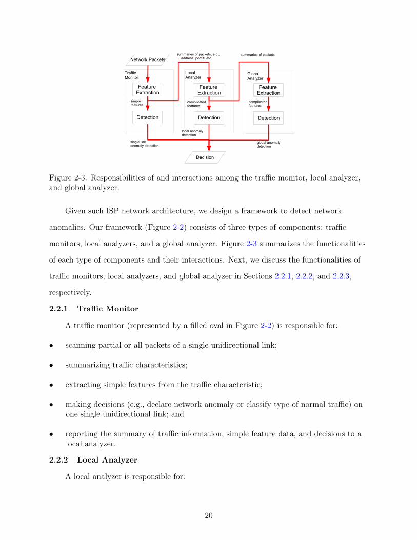
Figure 2-3. Responsibilities of and interactions among the traffic monitor, local analyzer,and global analyzer.

Given such ISP network architecture, we design a framework to detect network

anomalies. Our framework (Figure 2-2) consists of three types of components: traffic

monitors, local analyzers, and a global analyzer. Figure 2-3 summarizes the functionalities

of each type of components and their interactions. Next, we discuss the functionalities of

traffic monitors, local analyzers, and global analyzer in Sections 2.2.1, 2.2.2, and 2.2.3,

respectively.

2.2.1 Traffic Monitor

A traffic monitor (represented by a filled oval in Figure 2-2) is responsible for:

• scanning partial or all packets of a single unidirectional link;

• summarizing traffic characteristics;

• extracting simple features from the traffic characteristic;

• making decisions (e.g., declare network anomaly or classify type of normal traffic) onone single unidirectional link; and

• reporting the summary of traffic information, simple feature data, and decisions to alocal analyzer.

2.2.2 Local Analyzer

A local analyzer is responsible for:

20

• extracting complicated features from traffic information obtained at a single edgerouter;

• making decisions based on local traffic information (i.e., one edge router);

• reporting decisions, feature data, and summary of traffic information (if necessary) toa global analyzer.

The local analyzer can utilize temporal correlation of traffic to generate feature data.

2.2.3 Global Analyzer

A global analyzer is responsible for:

• extracting complicated features that require global information, such as routinginformation, from traffic;

• analyzing feature data obtained from multiple local analyzers; and

• making decisions with global information obtained from multiple edge routers.

Figure 2-4. Example of asymmetric traffic whose feature extraction is done by the globalanalyzer.

The global analyzer has a global view of the whole network. Hence, it exploits

both temporal correlation and spatial correlation of traffic. Here it is important to note

that, some feature data must be obtained at the global analyzer if global information

is required. For example, in Figure 2-4, if the traffic from subnet A to server B passes

through edge router X, and the traffic from server B to subnet A passes through edge

21

router Y, then the so-called two-way matching features between subnet A and server B

shall be obtained at the global analyzer, which has the routing information of the ISP

network.

The advantages of our framework design are that:

1. it is deployed on edge routers instead of systems of end users, such that it can detectnetwork anomalies in the first place they enter an AS;

2. it has no burden on core routers;

3. it is flexible in that detection of network anomalies can be made both locally andglobally;

4. it is capable of detecting low volume network anomalies accurately by exploitingspatial correlations among edge routers.

The framework is designed to be an add-on service provided by ISP to protect end

users from network anomalies.

2.3 Summary

This chapter is concerned with design of network anomaly detection frameworks.

There are two types of frameworks (i.e., host-based and network based. Our design is of

the second type). Specifically, we designed a framework deployed on edge routers. It is

composed of three components, traffic monitors, local analyzers, and global analyzers.

This framework is flexible in that it can detect network anomalies from both local view

and global view of the network. By exploiting spatial correlations among edge routers, our

framework is capable of detecting low volume network anomalies.

22

CHAPTER 3FEATURES FOR NETWORK ANOMALY DETECTION

3.1 Introduction

Given the network anomaly detection framework we have established, the second

issue of network anomaly detection is feature extraction. Features for network anomaly

detection have been studied extensively in recent years. For example, Peng et al.[12]

proposed the number of new source IP addresses to detect DDoS attacks, under the

assumption that source addresses of IP packets observed at an edge router were relatively

static in normal conditions than those during DDoS attacks. Peng further pointed out

that the feature could differentiate DDoS attacks from the flash crowd, which represents

the situation when many legitimate users start to access one service at the same time.

For example, when many people watch a live sports broadcast over the Internet at the

same time. In both cases (DDoS attacks and the flash crowd), the traffic rate is high. But

during DDoS attacks, the edge routers will observe many new source IP addresses because

attackers usually spoof source IP addresses of attacking packets to hide their identities.

Therefore, this feature improves those DDoS detection schemes that rely on traffic rate

only. However, Peng et al.[12] focused on detection of DDoS attacks. It did not mention

other types of network anomalies. For example, when malicious users are scanning the

network, we can also observe high traffic rate but few new source IP addresses. It is

very important to differentiate network scanning from flash crowd because the former is

malicious but the latter is not. The two-way matching feature on different network layers

(Section 3.3.1) can tell not only the presence of network anomalies but also their cause.

Lakhina et al.[16] summarized the characteristics of network anomalies under different

causes. Its contribution is to help identify causes of network anomalies. For example,

during DDoS attacks, we can observe high bit rate, high packet rate, and high flow rate.

The source addresses are distributed over the whole IP address space. On the other hand,

during network scanning, all the three rates are high, but the destination addresses,

23

rather than the source addresses, are distributed. However, the paper did not resolve an

important problem, i.e., how to extract features efficiently to match a high line rate in

the order of Gb/s. We proposed a data structure called Bloom filter array to address this

problem.

3.2 Hierarchical Feature Extraction Architecture

Network anomaly detection is not an easy task, especially at high-speed routers.

One of the main difficulties arises from the fact that the data rate is too high to afford

complicated data processing. An anomaly detection algorithm usually works with traffic

features instead of the original traffic data itself. Traffic features can be regarded as

succinct representations of the voluminous traffic, e.g., the traffic data rate is a feature of

the traffic.

We focus on presenting our feature extraction architecture for network anomaly

detection. We also cover extraction schemes for some simple features, such as data rate

and SYN/FIN(RST) ratio. The more advanced features, the so-called two-way matching

features, are discussed later.

3.2.1 Three-Level Design

Figure 3-1. Hierarchical structure for feature extraction.

To efficiently extract features from traffic, we design a three-level hierarchical

structure (Figure 3-1), where incoming packets are processed by level-one filters, then

by level-two filters, and finally by (level-three) feature extraction modules. Level-one filters

24

and level-two filters are placed in traffic monitors. A feature extraction module can be

placed in either a traffic monitor or a local analyzer, depending on the type of the feature.

Level-one filters select a packet based on its source-destination pair, which is defined

by the source IP address (SA), the source network mask (SNM), the destination IP

address (DA) , the destination network mask (DNM). For example, if we are interested in

packets from 172.10.5.28 to 210.33.68.102, we can choose 255.255.255.255 as both the SNM

and the DNM; if we are interested in packets from 172.10.x.x to 208.33.1.x, we can use

255.255.0.0 as the SNM and 255.255.255.0 as the DNM. In this way, we selectively monitor

an end-host or a subnet, giving much flexibility in framework configuration. The output of

a level-one filter is packets with the same source-destination pair, which are conveyed to

level-two filters.

A level-two filter classifies the packets coming from level-one filters, based on

the upper-layer1 data fields, e.g., TCP SYN or FIN. The packets of interest will be

forwarded to one or multiple feature extraction modules. For example, the number of

TCP SYN packets can be used to generate both the TCP SYN rate feature and the TCP

SYN/FIN(RST) ratio feature; hence, TCP SYN packets are conveyed to both the TCP

SYN rate module and the TCP SYN/FIN(RST) ratio module (Figure 3-1). On the other

hand, a feature module may need packets from multiple level-two filters. For example, the

SYN/FIN(RST) ratio feature extraction requires packets from three filters (Figure 3-1).

Compared to the packet classification schemes developed by Wang et al.[11] and

Peng et al.[12], our hierarchical structure for feature extraction is more general and

efficient.

Next, we describe the most important module in the three-level hierarchical structure,

the feature extraction module.

1 Here, the upper layer can be either Layer 4 or Layer 7.

25

Similar to previous studies [11, 12], we generate features in a discrete manner, i.e.,

our feature extraction module will generate a (feature) value or a vector at the end of

each time slot. Intuitively, shorter slot duration may reduce the detection delay, which

is defined as the interval from the epoch when the anomaly starts to the epoch when the

anomaly is detected; but a smaller duration may increase the computational complexity,

since the detection algorithm needs to analyze more feature data for the same time

interval. On the other hand, if a feature is represented by a ratio, the slot duration

must be sufficiently large to avoid division by zero. For example, if we want to use the

SYN/FIN(RST) ratio as in Ref. [11] to detect TCP SYN flood, then the slot duration

cannot be too small, because the number of FIN packets in a short period can be 0, which

will result in a false alarm even if the number of SYN packets is not large.

Feature extraction can be done in a traffic monitor, a local analyzer, and a global

analyzer, which will be described in Sections 3.2.2 and 3.2.3, respectively.

3.2.2 Feature Extraction in a Traffic Monitor

As we mentioned earlier, some features are generated within a traffic monitor. These

features are typically simple and reside in traffic of a single unidirectional link.

In our framework, a traffic monitor can generate the following features:

• Packet rate: defined by the number of packet arrivals in one time slot. This feature issimple but useful for detecting high volume DoS and DDoS attacks. But it can hardlyhelp detect low volume attacks and other types of network anomalies. Furthermore,normal network behaviors may be also accompanied with high packet rate, e.g., flashcrowd [12]. So is data rate.

• Data rate: defined by the total number of bits of all packets that arrive in one timeslot.

• SYN/FIN(RST) ratio2 : defined by the ratio of the number of TCP SYN packets inone time slot to the number of FIN (and a portion of RST) packets in the same timeslot.

2 How to obtain this ratio can be found in Ref. [17].

26

3.2.3 Feature Extraction in a Local Analyzer or a Global Analyzer

Although a traffic monitor can generate simple features efficiently, these features may

not be sufficient to detect network anomalies. In particular, the packet rate and data

rate features may only be useful for detecting network anomalies accompanied with high

volume traffic; and SYN/FIN(RST) ratio has a large variation even for normal traffic

and hence cannot help accurately distinguish normal network conditions from network

anomalies. To improve detection accuracy, one can use a local analyzer to generate more

sophisticated features, for example, the SYN/SYN-ACK ratio proposed in Ref. [17] and

the percentage of new IP addresses proposed in Ref. [12].

However, the existing features such as the SYN/SYN-ACK ratio [17] and the

percentage of new IP addresses [12] either do not lead to good performance of detectors,

or require high storage/time complexity (Section 3.1). To address these deficiencies, we

propose a new type of features called two-way matching features, which can make distinct

features between normal and attack traffic, thereby improving accuracy of detecting

attacks.

Next, we discuss the two-way matching features and the extraction scheme.

3.3 Two-Way Matching Features

3.3.1 Motivation

The motivation of using two-way matching features arises from the fact that, for

most Internet applications, packets are generated from both end hosts that are engaged

in communication. Information carried by packets on one direction shall match the

corresponding information carried by packets on the other direction. By monitoring the

degree of mismatch between flows of two directions, we can detect network anomalies.

To illustrate this, let us consider the behaviors of the two-way traffic in three scenarios,

namely, 1) normal conditions, 2) DDoS attacks, and 3) re-route.

In the first scenario, when the network of an ISP works normally, information carried

on both directions of communication matches (Figure 3-2). Host a and host v are two

27

Figure 3-2. Network in normal condition.

ends of communication (assume that host v is within the autonomous system of the ISP

while host a is not). Host a sends a packet to host v and v responds a packet back to

host a. Both packets pass the edge router A. From the point of view of the local analyzer

1 attached to edge router A, we define the first packet as an inbound packet, and the

second packet as an outbound packet. The source IP address (SA) and destination IP

address (DA) of the inbound packet match the DA and SA of the outbound packet. If the

communication is based on UDP or TCP, we can further observe that the source port (SP)

and destination port (DP) of the inbound packet match the DP and SP of the outbound

packet. Therefore, the local analyzer 1 can observe matched inbound and outbound

packets in normal conditions. In the example of Figure 3-2, it is assumed that the border

gateway protocol (BGP) routing makes the inbound packets and the corresponding

outbound packets pass through the same edge router. If the BGP routing makes the

inbound packets and the corresponding outbound packets go through different edge routers

(Figure 2-4), the matching can still be achieved by a global analyzer (Section 2.2.3), i.e.,

multiple local analyzers convey the unmatched inbound packets and the corresponding

outbound packets to the global analyzer, which has the routing information of the whole

autonomous system.

28

Figure 3-3. Source-address-spoofed packets.

In the second scenario, when attackers launch spoofed-source-IP-address DDoS

attacks[18], the local analyzer 1 observes many unmatched inbound packets (Figure 3-3).

Since source addresses of inbound packets are spoofed, the outbound packets are routed to

the nominal destinations, i.e., b and c in Figure 3-3, which do not pass through edge router

A any more. In this case, local analyzer 1 will observe many unmatched inbound packets.

Figure 3-4. Reroute.

In the third scenario (Figure 3-4), the number of unmatched inbound packets

observed by local analyzer 1 is increased due to a failure of the original route and re-route

of outbound packets to another edge router. A global analyzer can address this problem

similar to the asymmetric case in the first scenario.

29

All the above scenarios seem to suggest that the number of unmatched inbound

packets observed by an edge router is a good feature for network anomaly detection.

However, usually, this is not true because traffic volume from one end to the other is not

symmetric, typically. In Figure 3-2, if host a is a client uploading a large file using the File

Transfer Protocol (FTP)[19] to host v, there will be much more packets from a to v than

those from v to a. Uploading file to an FTP server is a normal behavior but the number of

unmatched inbound packets is very high in this case.

Therefore, it is more appropriate to use flow-level quantities (instead of packet-level

quantities) as features for network anomaly detection. As in the above FTP case, when a

TCP connection is established, all packets on one direction constitute one flow and packets

on the reverse direction constitute another flow. No matter how many packets are sent on

each direction, there are only one inbound flow and only one outbound flow. They match

in IP addresses and port numbers. Therefore, we call the number of unmatched inbound

flows as a two-way matching feature.

Two-way matching features are shown to be effective indicators of network anomalies

[20].3 However, extraction of two-way matching features at high-speed edge routers is not

an easy task. We will address this issue in Sections 3.4 and 3.5.

Next, we define the two-way matching features.

3.3.2 Definition of Two-Way Matching Features

We first define three terms.

Definition 1. Signature is the information of interest, carried in traffic.

The exact definition of signature depends on the specific application targeted. For

example, to detect SYN flood DDoS attacks, we may use a 5-tuple signature <SA, SP,

3 Two-way matching features are good indicators of DDoS attacks with spoofed sourceIP addresses but are not good indicators of DDoS attacks with non-spoofed source IPaddresses.

30

DA, DP, sequence number> for inbound packets and <DA, DP, SA, SP, ACK number –

1> for outbound packets. We further define inbound signature as the signature extracted

from inbound packets and outbound signature from outbound packets.

Definition 2. A flow is a set of the packets with the same signature and the same

direction.

For example, a TCP connection between two ends generates two flows with different

directions.

Definition 3. An unmatched inbound flow (UIF) is an inbound flow that has no cor-

responding outbound packet arriving at an intended edge router within a time period

Γ.

Note that we use a time constraint Γ in the definition of UIF because it takes

time for an outbound packet to arrive. If Γ is too short, then some returning outbound

packets might be ignored, which increases the false alarm probability of network anomaly

detection. If Γ is too large, then the detection delay is long. The suitable choice of Γ

depends on the round trip time (RTT) of the connection. For example, we can choose Γ

to be the most significant 99% RTT, i.e., more than 99% corresponding outbound packets

return within time Γ.

Table 3-1: Notations for two-way matching featuresNotation Descriptionti The ith sampling time epoch, where ti+1 = ti + Γ and i ∈ Z+.s(p) Inbound signature of an an inbound packet p.s′(p′) Outbound signature of an outbound packet p′.D(ti) The number of UIF during the ith period.

Based on the above definitions, we define the two-way matching features to be the

number of UIF. Table 3-1 lists the notations used in the rest of the paper, where Z+

stands for the nonnegative integer set.

In the following sections, we present algorithms to extract two-way matching features

from the traffic at local analyzers. Note that two-way matching features should be

31

extracted by global analyzers when an AS is not symmetric. However, the feature

extraction approaches used by local analyzers and global analyzers are same.

3.4 Basic Algorithms

This section presents two basic algorithms to process and store the two-way matching

features, namely, the hash table algorithm and the Bloom filter algorithm.

3.4.1 Hash Table Algorithm

The general procedure to extract the two-way matching features from traffic at an

local analyzer is:

1. The local analyzer maintains a buffer in memory;

2. When the traffic monitor captures an inbound packet, if its inbound signature is notin the buffer, the local analyzer creates one entry for its signature and set the state ofthat entry to “UNMATCHED”;

3. When the traffic monitor captures an outbound packet, if its outbound signature is inthe buffer, the local analyzer sets the state of that entry to “MATCHED”;

4. At time ti+1, the local analyzer assigns the number of entries with state “UNMATCHED”to D(ti).

So typically we need three operations: insertion, search and removal4 .

A basic algorithm to do this is to use a hash table. Suppose the signature extracted

from a packet is b bits long. We organize the buffer into a table, V , with ` cells of b + 1

bits each. The extra one bit is the state bit. We also have K hash functions hi:S 7→ Z`,

where i ∈ ZK = 0, 1, . . . ,K − 1, and S is the data set of interest, e.g., signature domain.

The symbol Z` stands for the set 0, . . . , `− 1, where ` is an integer.

The operations of hash table algorithm are listed in Figure 3-5, where the argument s

is the signature extracted from a packet.

4 Setting the state to “MATCHED” is actually the removal operation.

32

1. function HashTableInsert(V , s)2. for i ← 0 to K − 13. if V [hi(s)] is empty4. insert s to V [hi(s)], set state bit of V [hi(s)] to “UNMATCHED”5. return6. end if7. end for8. report insertion operation error9. end function

10. function HashTableSearch(V , s)11. for i ← 0 to K − 112. if V [hi(s)] is empty13. return false14. if V [hi(s)] holds s15. return true16. end for17. return false;18. end function19. function HashTableRemove(V , s)20. for i ← 0 to K − 121. if V [hi(s)] is empty22. return;23. if V [hi(s)] holds s24. set state bit of V [hi(s)] to “MATCHED”25. return true;26. end if27. end for28. end function

Figure 3-5. Hash Table Algorithm

3.4.2 Bloom Filter

The hash table algorithm can be used for offline traffic analysis or analysis of low

data-rate traffic but it cannot catch up with a high data rate at edge routers. To address

this limitation, one can use Bloom filter algorithm[21]. Compared to the hash table

algorithm, Bloom filter algorithm reduces space/time complexity by allowing small degree

of inaccuracy in membership representation, i.e., a packet signature, which does not

appear before, may be falsely identified as present.

33

Bloom filter stores data in a vector V of M elements, each of which consists of one

bit. Bloom filter also uses K hash functions hi:S 7→ ZM , where i ∈ ZK. Figure 3-6

describes the insertion and search operations of Bloom filter.

1. function BloomFilterInsert(V , s)

2. for ∀i ∈ ZK do

3. V [hi(s)] ← 1

4. end function

5. function BloomFilterSearch(V , s)

6. for ∀i ∈ ZK do

7. if V [hi(s)] 6= 1 then

8. return false

9. end for

10. return true

11. end function

Figure 3-6. Bloom Filter Operations

(a) (b)

Figure 3-7. Scenarios of the problems caused by Bloom filter. (a) Boundary problem. (b)An outbound packet arrives before its matched inbound packet with t2 − t1 < Γ.

Although Bloom filter has better performance in the sense of space/time trade-off, it

cannot be directly applied to our application because of the following problems:

1. Bloom filter does not provide removal functionality. Since one bit in the vector maybe mapped by more than one item, it is unsuitable to remove the item by setting allbits indexed by its hash results to 0.

2. Bloom filter does not have counting functionality. Although the counting Bloom filter[22] can be used for counting, it replaces a bit with a counter, which significantlyincreases the space complexity.

34

3. Sampling two-way matching features in discrete time results in boundary effect(Figure 3-7(a)). An inbound packet arrives at time t′1 ∈ [ti, ti+1) whereas its matchedoutbound packet arrives within next period. The inbound packet is counted as anunmatched inbound packet even though t′2 − t′1 < Γ. Therefore, boundary effectincreases the false alarm rate.

4. In previous discussion, we did not consider the scenario that an outbound packet mayarrive before its matched inbound packet (Figure 3-7(b)). When the outbound packetarrives at time t′1, its signature is not in the buffer, so we do nothing. At time t′2,its matched inbound packet arrives, whose inbound signature will be recorded. As aresult, the latter is regarded as an unmatched inbound packet during period [ti, ti+1).This early-arrival problem also increases the false alarm rate.

Next, we propose a Bloom filter array algorithm to address the above problems.

3.5 Bloom Filter Array (BFA)

The good space/time trade-off motivates us to apply Bloom filter to two-way

matching feature extraction. But we need to address the limitations of Bloom filter

mentioned in Section 3.4.2. Our idea is to design a Bloom filter array (BFA) with the

following functionalities, not available in the original Bloom filter [21, 23]:

1. Removal functionality : We implement insertion and removal operations synergisticallyby using insertion-removal pair vectors. The trick is that, rather than removing anoutbound signature from the insertion vector, we create a removal vector and insertthe outbound signature into the removal vector.

2. Counting functionality : We implement this by introducing counters in Bloomfilter array. The value of a counter is changed based on the query result from aninsertion/removal operation.

3. Boundary effect abatement : We use multiple time slots and a sliding window tomitigate the boundary effect.

4. Resolving the early-arrival problem: which is achieved by storing signature of not onlyinbound packets but also outbound packets. In this way, when an inbound packetarrives and the signature of its matched outbound packet is present, we do not countthis inbound packet as an unmatched one.

3.5.1 Data Structure

To address the boundary effect, we partition the time constraint Γ into w time slots,

where w is the number of slots enough to mitigate the boundary effect (see Section 3.5.3).

35

Assume the length of a slot is γ. Then, we have Γ = w × γ. The data structure of BFA is

as follows:

• An array of bit vectors IVj (j ∈ Z+), where IVj is the jth insertion vector holdinginbound signatures in slot [τj, τj+1), where τj+1 = τj + γ.

• An array of bit vectors RVj (j ∈ Z+), where RVj is the jth removal vector holdingoutbound signatures in slot [τj, τj+1).

• An array of counters Cj (j ∈ Z+), where Cj is used to count the number of UIF inslot [τj, τj+1).

Since the two-way flows need to be matched within a time interval of length Γ, we

only need to keep information within a time window of length Γ. That is, if the current

slot is [τj, τj+1), only IVj−w+1, . . . , IVj, RVj−w+1, . . . , RVj, and Cj−w+1, . . . , Cj are

kept in memory.

3.5.2 Algorithm

Our algorithm for BFA (Figure 3-8) consists of three functions, namely, ProcInbound,

ProcOutbound and Sample, which are described as below.

Function ProcInbound is to process inbound packets. It works as below. When

an inbound packet arrives during [τj, τj+1), we increase Cj by 1 and insert its inbound

signature s into IVj if none of the following conditions is satisfied:

1. s is stored in at least one RVj′ , where j − w + 1 ≤ j′ ≤ j;

2. s is stored in IVj.

Condition 1 being true means that the corresponding outbound flow of this inbound

packet has been observed previously; so we should not count it as an unmatched inbound

packet. Condition 2 being true means that the inbound flow, to which this inbound packet

belongs, has been observed during the current slot j; so we should not count the same

inbound flow again. If both conditions are false, we increase Cj by one to indicate a new

potential UIF (line 7 to 10).

36

1. function ProcInbound(s)2. a ← false, b ← false3. if ∃j′, j − w + 1 ≤ j′ ≤ j, such that BloomFilterSearch(RVj′ ,s) returns true then4. a ← true5. if BloomFilterSearch(IVj,s) returns true then6. b ← true7. if a and b are both false8. Cj ← Cj + 19. BloomFilterInsert(IVj, s)

10. end if11. end function12. function ProcOutbound(s′)13. for j′ ← j to j − w + 114. if BloomFilterSearch(RVj′ , s

′) returns true15. break16. if BloomFilterSearch(IVj′ , s

′) returns true17. Cj′ ← Cj′ − 118. end for19. BloomFilterInsert(RVj, s′)20. end function21. function Sample(j)22. return Cj−w+1

23. end function

Figure 3-8. Bloom Filter Array Algorithm

Function ProcOutbound is to process outbound packets. It works as below. When an

outbound packet arrives during [τj, τj+1), we check whether we need to update counter Cj′

for each j′ (j − w + 1 ≤ j′ ≤ j). Specifically, for each j′ (j − w + 1 ≤ j′ ≤ j), decrease Cj′

by one if its outbound signature s′ satisfies both of the following conditions:

1. s′ is not contained in RVj′ ;

2. s′ is contained in IVj′ .

Condition 1 being true means that no packet from the outbound flow to which this

outbound packet belongs arrives during the j′th time slot. Condition 2 being true means

that the matched inbound flow of this outbound packet has been observed in the j′th slot.

Satisfying both conditions means that its matched inbound flow has been counted as a

potential UIF; hence, upon the arrival of the outbound packet, we need to decrease Cj′ by

37

one to uncount it. In Function ProcOutbound, Line 13 starts a loop to iterate j′ from j to

j − w + 1. Condition 1 is checked in lines 14 to 15 and Condition 2 is checked in lines 16

to 17. Note that the loop exits (line 15) if RVj′ contains s′; this is because an outbound

packet of the same flow arrived in that j′th slot and hence the buffer of the jth slot (for

each j < j′) has already been checked.

Function Sample is to extract the two-way matching features. When we execute

Function Sample at the end of the jth slot (i.e., at time τj+1), the output is D(τj−w+1)

instead of D(τj) since a time lag of Γ (w slots) is needed for two-way matching.

3.5.3 Round Robin Sliding Window

1. function ProcInbound(s)2. a ← false, b ← false3. if ∃j′, j′ ∈ (I − w + 1)%w, (I − w + 2)%w, . . . , I%w, such that

BloomFilterSearch(RVj′ ,s) returns true then4. a ← true5. if BloomFilterSearch(IVI ,s) returns true then6. b ← true7. if a and b are both false then8. CI ← CI + 19. BloomFilterInsert(IVI , s)

10. end if11. end function12. function ProcOutbound(s′)13. for j′ ← I to (I − w + 1)%w14. if BloomFilterSearch(RVj′ , s

′) returns true then15. break16. if BloomFilterSearch(IVj′ , s

′) returns true then17. Cj′ ← Cj′ − 118. end for19. BloomFilterInsert(RVI , s′)20. end function21. function Sample()22. I ← (I + 1)%w23. return CI

24. end function

Figure 3-9. Bloom Filter Array Algorithm using sliding window

The algorithm presented in Section 3.5.2 has a drawback in memory allocation.

Specifically, at epoch τj+1, we sample D(τj−w+1), and then we need to throw away the

38

buffer for the (j − w + 1)th slot, and create a new buffer for the (j + 1)th slot. This is

inefficient for most operating systems. A better memory allocation strategy is to use the

useless buffer of the (j−w +1)th slot for the new (j +1)th slot, saving the cost of memory

allocation. This is the idea of our round-robin sliding window.

Our new memory allocation scheme is the following. We allocate a memory area

of fixed size for w insertion vectors IVj, w removal vectors, RVj, and w counters

Cj, where j ∈ Zw. The insertion vector, removal vector, and counter for the jth slot

are IVj%w, RVj%w, and Cj%w, respectively. Here, % stands for modulo operation. We

also define a pointer I to point to the current slot. Then, rather than deleting a useless

buffer and acquiring a new buffer for the new slot, we simply update the pointer by

I = (I + 1)%w. Figure 3-9 shows the improved version of BFA, based on the round-robin

sliding window.

3.5.4 Random-Keyed Hash Functions

In previous sections, we assume K hash functions are given a priori. However,

choosing hash functions appropriately is not trivial due to the following two concerns.

First, K is a user-specified parameter, subject to change. But for a value of K that a

user5 chooses, it is not desirable to require the user to manually select K hash functions

from a large pool of hash functions provided by the manufacturer. Also, it wastes memory

to store a large pool of hash functions.

Second, to improve security, the K hash functions need to be changed over time.

Otherwise, if an attacker knows the hash functions, he can generate such attack packets

that for signatures of any two packets, s1 and s2, s1) 6= s2 but hi(s1) = hi(s2), i ∈ ZK. The

consequence is that even if there are many attack packets with different signatures, the

5 A user here is a network operator who wants to use our BFA and detection techniqueto detect network anomalies.

39

BFA algorithm will regard them as belonging to the same flow. So, the number of UIF for

these packets is only one. This causes security vulnerability.

We address the aforementioned two problems by using keyed hash functions, i.e.,

we only need one kernel hash function and K randomly generated keys. Specifically, the

ith hash function hi(x) is simply h(keyi, x), where h is a predefined kernel hash function

and keyi (i ∈ ZK) are randomly generated keys. For example, we can use MD5 Digest

Algorithm[24] as the hash function. Since MD5 takes any number of bits as input, we can

organize keyi and x into a bit vector and apply MD5 to it.

Using keyed hash functions, the first concern (varying K) can be addressed straightforwardly.

Specifically, when K is changed, we simply generate a corresponding number of random

keys. Applying these K keys to the same kernel hash function, we obtain K hash

functions. Hence, our method has two advantages: 1) the number of hash functions

can be specified on the fly; 2) hash functions are determined on the fly, instead of being

stored a priori, resulting in storage saving.

The second concern (changing hash functions) can also be addressed if the keys are

periodically changed. Even if the kernel hash function is disclosed, it is still very difficult,

if not impossible, for an attacker to guess the changing random keys.

Note that the collision probability of the hash functions is not affected due to the

use of keyed hash functions. In the case of random-keyed hash functions, the collision

probability of hi(x) depends on not only the collision probability of h but also the

correlation between keyi and x. Since random number generator techniques are so mature

that we can assume independence between keyi and x, introduction of random keys has no

effect on the collision probability.

3.6 Complexity Analysis

This section compares the hash table, Bloom filter, and our BFA. The section is

organized as follows. In Section 3.6.1, we analyze the space/time trade-off for the three

algorithms. Section 3.6.2 addresses how to optimally choose parameters of BFA.

40

3.6.1 Space/Time Trade-off

Space/time trade-off for both Hash table and Bloom filter algorithms was analyzed by

Bloom [21]. However, the analysis by Bloom[21] is not directly applicable to our setting

due to the following reasons:

1. A static data set was assumed by Bloom[21]. However, our feature extraction dealswith a dynamic data set, i.e., the number of elements in the data set changes overtime. Hence, new analysis for a dynamic data set is needed. In addition, Bloom[21]only considered the search operation due to the assumption of static data sets. Ourfeature extraction, on the other hand, requires three operations, i.e., insertion, search,and removal, for dynamic data sets.

2. Bloom[21] assumed bit-comparison hardware in time complexity analysis. However,current computers usually use word (or multiple-bit) comparison, which is moreefficient than bit-comparison hardware. Hence, it is necessary to analyze thecomplexity based on word comparison.

3. The time complexity obtained by Bloom[21] did not include hash function calculations.However, hash function calculation dominates the overall time complexity, e.g.,calculating one hash function based on MD5 takes 64 clock cycles [25], while oneword-comparison usually takes less than 8 clock cycles [26].

For the above reasons, we develop new analysis for the hash table and Bloom filter,

respectively. In addition, we analyze the performance of BFA and use numerical results to

compare the three algorithms. Table 3-2 lists the notations used in the analysis.

Table 3-2: Notations for complexity analysisNotation DescriptionN Random variable representing the number of different flows recorded.φ Empty ratio.η Collision probability, i.e., the probability that an item is falsely identified

to be in the buffer.R Flow arrival rate, which is assumed to be constant.

Analysis for hash table. Denote by Mh the size of a hash table in bits (i.e., space

complexity) and by Th the random variable representing the number of hash function

calculations for an unsuccessful search (i.e., time complexity).

Let us consider search operation first. Upon the arrival of an inbound packet, the

HashTableSearch (see Figure 3-5) checks if its inbound signature s is in the table. Because

41

an unsuccessful search will continue the loop until an empty cell is found, it consumes

more time than a successful one does. In addition, it is very difficult to analyze the time

complexity of a successful search since the complexity depends on the distribution of

flow signatures and the data rate of each flow. For this reason, we only consider the time

consumed for an unsuccessful search, which is a conservative estimate of the average time

complexity of a search. Recall that, as mentioned in Section 3.4.1, the hash table has `

cells of b + 1 bits each, such that Mh = `(b + 1). Given the condition that N flows have

been recorded by the hash table, the empty ratio is

φ =`−N

`=

Mh −N(b + 1)

Mh

. (3–1)

In each loop, the HashTableSearch calculates one hash function and checks the addressed

entry. If the entry is not empty, next loop is executed. The conditional probability that

the loop is executed for x times for a given n follows a geometric distribution as below

Pr[Th = x|N = n] = φ(1− φ)x−1. (3–2)

Therefore the conditional expectation of Th is

E[Th|N = n] =∞∑

x=1

xφ(1− φ)x−1 =1

φ=

Mh

Mh − n(b + 1). (3–3)

Since the table records data for the duration of Γ, the maximum number of different

flows that we need to store in the buffer is RΓ. Then the expectation of Th is

E[Th] =RΓ∑n=0

Pr[N = n]E[Th|N = n]. (3–4)

Assume N has a uniform distribution

Pr[N = n] =1

RΓ + 1. (3–5)

42

Applying Equation (3–5) to Equation (3–4), we obtain the expectation of Th

E[Th] =1

RΓ + 1

RΓ∑n=0

Mh

Mh − n(b + 1). (3–6)

Since the time to insert a signature into or remove a signature from a given entry is

much shorter than that to find the proper entry, the time complexities of insertion and

removal operations are almost the same as that of the search operation. Equation (3–6)

gives the space/time trade-off (i.e., Mh vs. Th) of the hash table method.

Analysis for Bloom filter. First of all, we consider the space complexity of Bloom

filter. Denote by Mb the length of the vector V used by Bloom filter (see Section 3.4.2).

The choice of Mb will affect the accuracy of the search function, BloomFilterSearch (see

Figure 3-6). The reason is the following.

When signatures of N flows are stored in V , φ, denoting the percentage of entries of

V with value 0, is

φ =

(1− K

Mb

)N

, (3–7)

where K is the number of hash functions. Assuming K ¿ Mb, as is certainly the case, we

can approximate φ as

φ ≈ exp

(−KN

Mb

). (3–8)

Function BloomFilterSearch(V , s) falsely identifies s to be stored in V if and only if

results of all K hash functions point to bits with value 1, which is known as a collision.

Denote by ηN the collision probability under the condition that N flows have been

recorded. Then

ηN = (1− φ)K =

[1− exp

(−KN

Mb

)]K. (3–9)

43

Therefore, the average collision probability is

η =RΓ∑n=0

ηn Pr[N = n] =1

RΓ + 1

RΓ∑n=0

[1− exp

(−Kn

Mb

)]K, (3–10)

where N is assumed to be uniformly distributed as in Equation (3–5). From Equation (3–10),

it can be observed that η decreases with Mb if K is fixed. Based on Equation (3–10), we

can denote Mb as a function of η and K as below

Mb = αRΓ(η,K). (3–11)

Equation (3–11) gives the space complexity of Bloom filter as a function of collision

probability and the number of hash functions.

Now, let us consider the time complexity of Bloom filter. Denote by Tb the random

variable representing the number of hash function calculations.

Function BloomFilterInsert always calculates all the K hash functions, that is,

Tb|BloomFilterInsert is executed ≡ K, (3–12)

where “|” followed by an event means a condition and “≡” means equality with

probability 1.

For function BloomFilterSearch, we first consider a special case that BloomFil-

terSearch returns true. In this case, all K hash functions need to be calculated. So

Tb|BloomFilterSearch returns true ≡ K. (3–13)

This fact will be used in the analysis for BFA (see Section 3.6.1).

In general,

Pr[Tb = x|N=n and BloomFilterSearch is executed]

=

φ(1− φ)x−1 x < K

(1− φ)K−1 x = K. (3–14)

44

Hence, the conditional expectation of Tb is

E[Tb|N=n and BloomFilterSearch is executed]

=K−1∑x=1

xφ(1− φ)x−1 +K(1− φ)K−1

=1−

[1− exp

(− Kn

αRΓ(η,K)

)]K

exp(− Kn

αRΓ(η,K)

)

4=βn(η,K). (3–15)

Averaging over N at both sides of Equation (3–15), we get the expectation of Tb under the

condition that BloomFilterSearch is executed, i.e.,

E[Tb|BloomFilterSearch is executed]

=1

RΓ + 1

RΓ∑n=0

βn(η,K). (3–16)

If we know the two prior probabilities, i.e., the probability that BloomFilterSearch is

executed, denoted by Ps, and the probability that BloomFilterInsert is executed, denoted

by Pi, then we can get

E[Tb] =Ps

RΓ + 1

RΓ∑n=0

βn(η,K) + PiK. (3–17)

Equation (3–17) gives the time complexity of Bloom filter in terms of number of hash

function calculations.

Analysis for Bloom filter array. Once again, we analyze the space complexity

of BFA first. The techniques in Section 3.6.1 can be applied here since BFA is originated

from standard Bloom filter. However, there are some differences between these two

schemes. As described in Section 3.5, BFA has multiple buffers such as IVj, RVj, and Cj,

j ∈ Zw. Therefore, the storage size for BFA, denoted by Ma (in bits), is w(2 ×Mv + L),

where Mv is the size of each insertion or removal vector, and L is the size of each counter

in bits.

45

Similar to Equation (3–10), the collision probability is

η =1

Rγ + 1

Rγ∑n=0

[1− exp

(−Kn

Mv

)]K. (3–18)

Note that length of each time slot of BFA is γ, so that the upper limit of the summation

operator is Rγ rather than RΓ. Similar to Equation (3–11), Mv is a function of η and K.

We define

Mv = αRγ(η,K). (3–19)

Then

Ma = w(2× αRγ(η,K) + L). (3–20)

Equation (3–20) gives the space complexity of BFA.

Now, let us consider the time complexity of BFA. Denote by Ta the random

variable representing the number of hash function calculations for BFA. Recall that BFA

(Figure 3-9) defines three functions, ProcInbound, ProcOutbound, and Sample. Obviously,

Ta|Sample is executed ≡ 0. (3–21)

When executing Function ProcInbound, all the K hash functions need to be

calculated. The reason is the following.

1. If variables a and b are both false, Function BloomFilterInsert is executed, whichcalculates K hash functions (see Equation (3–12)).

2. Otherwise, at least one of a and b is true; then at least one of the search operations,i.e., BloomFilterSearch(RVj′ ,s), j′ = (I − w + 1)%w,(I − w + 2)%w,. . . , I%w, andBloomFilterSearch(IVI ,s), returns true. This also means that K hash functions havebeen calculated (see Equation (3–13)).

Therefore, in any case, ProcInbound calculates all the K hash functions. Further note

that, although BloomFilterSearch executes up to w + 1 search operations, and at most

one insertion operation, the total number of hash function calculations in these operations

46

is the same as that in one search operation. This is because the results of hash function

calculation in one search operation can be used again by all the other search operations

and insertion operation. Therefore,

Ta|ProcInbound is executed ≡ K. (3–22)

Similarly,

Ta|ProcOutbound is executed ≡ K. (3–23)

In each time slot, we execute Sample once, ProcInbound for Rpiγ times, and ProcOut-

bound for Rpoγ times, where Rpi and Rpo are inbound packet arrival rate and outbound

packet arrival rate, respectively. Combining Equations (3–21), (3–22), and (3–23) and

assuming (Rpi + Rpo)γ À 1, which is always true in our design of BFA, we have

E[Ta] =0× 1

(Rpi + Rpo)γ + 1+

K(Rpi + Rpo)γ

(Rpi + Rpo)γ + 1≈ K. (3–24)

Combining Equations (3–24) and (3–20), we obtain the relationship between Ma and

Ta as below

Ma = w [2αRγ(η, E[Ta]) + L] . (3–25)

Table 3-3: Space/time complexity for hash table, Bloom filter, and BFAAlgorithm Space complexity Time complexityHash table Mh (free variable) Equation (3–6)Bloom filter Equations (3–10) and (3–11) Equations (3–15), (3–16), and (3–17)BFA Equation (3–18), (3–19), and (3–20) Equation (3–24)

Table 3-3 lists the space complexity and time complexity for hash table, Bloom filter,

and BFA algorithms.

Numerical Results.

47

In this section, we use the formulae derived in above sections to compare the hash

table scheme with BFA algorithm through numerical calculations. The setting of our

numerical study is the following:

1. Traces captured from an ISP’s edge router shows that the average number offlows during one second is around 250, 000. So, we let R=250, 000. To reduce theprobability of false alarms caused by normal packets with long RTT, we choose Γlarge enough such that more than 99% packets have RTT less than Γ. For the sametraces, Γ=80 seconds.

2. Suppose we want to detect TCP traffic anomaly. Thus the signature captured fromeach packet is composed of 32-bit SA, 32-bit DA, 16-bit SP, and 16-bit DP. So b = 96bits.

3. In the BFA algorithm, we use 40 time slots (i.e., w = 40), each of which is 2 seconds(i.e., γ = 2). Also suppose each counter is a 32-bit integer (i.e., L = 32).

1 2 3 4 5 6 7 8 9 1010

7

108

109

1010

1011

Time E[T]

Spa

ce M

Hash Table

BFA (η = 0.001)

BFA (η = 0.01)

Figure 3-10. Space/time trade-off for the hash table, BFA with η = 0.1%, and BFA withη = 1%

Figure 3-10 shows M vs. E[T ] for the hash table scheme, BFA with collision

probability 1%, and BFA with collision probability 0.1%. In Figure 3-10, X axis represents

the time complexity (i.e., the expected number of hash function calculations) and Y

axis represents the space complexity (i.e., the number of bits needed for storage). From

Figure 3-10, we can see that the curve of BFA is below the curve of the hash table. It

means BFA uses less space for a given time complexity. Therefore, BFA achieves better

48

space/time trade-off than the hash table. We also see that the curve of BFA with η = 1%

is below the curve of BFA with η = 0.1%. This shows the relationship between space/time

and collision probability. Specifically, to reach a lower collision probability or more

accurate detection, we need to either calculate more hash functions or use more storage

space.

To see the gain of using BFA, let us look at an example. Suppose E[T ] = 5, i.e., in

each slot, 5 hash function calculations is needed on average. Then, the memory required

by the hash table scheme, BFA with η = 0.1%, and BFA with η = 1% is 1.01G bits,

115.3M bits, and 62.9M bits, respectively. It can be seen that our BFA with η = 1% can

save storage by a factor of 16, compared to the hash table scheme.

Figure 3-10 shows that for the hash table scheme, Mh is a monotonic decreasing

function of E[Th]. The observation matches our intuition that the larger table, the smaller

collision probability for hash functions, resulting in less hash function calculations. Further

note that Mh approaches RΓ(b + 1) when E[Th] increases. This is the minimum space

required to tolerate up to RΓ flows.

For BFA, Ma is not a monotonic function of E[Ta], which approximately equals K.

We have the following observations.

• Case A: For fixed storage size, the smaller K, the larger the probability that all Khash functions of two different inputs return the same outputs, which is the collisionprobability. In other words, the smaller K, the larger storage size required to achievea fixed collision probability. That is, K ↓⇒ Ma ↑.

• Case B: Since an input to BFA may set K bits to “1” in a vector V , hence the largerK, the more bits in V will be set to “1” (nonempty), which translates into a largercollision probability. In other words, the larger K, the larger storage size required toachieve a fixed collision probability. That is, K ↑⇒ Ma ↑.Combining Cases A and B, it can be argued that there exists a value of K or E[Ta]

that achieves the minimum value of Ma, given a fixed collision probability. This minimum

property can be used to guide the parameter setting for BFA, which will be addressed in

Section 3.6.2.

49

3.6.2 Optimal Parameter Setting for Bloom Filter Array

This section addresses how to determine parameters of BFA under two criteria,

namely, minimum space criterion and competitive optimality criterion.

Minimum space criterion. According to Equation (3–25), three parameters, Ma,

E[Ta], and η, are coupled. Since the collision probability η critically affects the detection

error rate in our network anomaly detection, a network operator may want to choose an

upper bound η on the acceptable collision probability η and then minimize the storage

required, i.e.,

minE[Ta]

Ma, subject to η ≤ η (3–26)

According to Equation (3–25), the solution of (3–26) is as below

M∗a = min

E[Ta]Ma = min

E[Ta]w [2αRγ(η, E[Ta]) + L] , (3–27)

E[Ta]∗ = arg min

E[Ta]Ma = arg min

E[Ta]αRγ(η, E[Ta]). (3–28)

10−5

10−4

10−3

10−2

10−1

1

2

3

4

5

6

7

8x 10

8

η

Ma*

(a)

10−5

10−4

10−3

10−2

10−1

2

4

6

8

10

12

14

η

E[T

a]*

(b)

Figure 3-11. Relation among space complexity, time complexity, and collision probability.(a) M∗

a vs. η. (b) E[Ta]∗ vs. η.

Figure 3-11 shows M∗a vs. η, and E[Ta]

∗ vs. η under the same setting as that

in Section 3.6.1. From Figure 3-11(a), it can be observed that M∗a decreases when η

50

increases. This is because the larger collision probability we can tolerate, the less space

required.

From Figure 3-11(b), one observes that generally, E[T ∗a ] decreases when η increases.

This may be because the smaller E[T ∗a ] or K, the larger the probability that all K hash

functions of two different inputs return the same outputs, which is the collision probability.

Competitive optimality criterion.From Equation (3–18), it can be observed that

η decreases with the increase of Mv if K is fixed; in other words, Mv decreases with the

increase of η if K is fixed. Further, from Equations (3–19) and (3–25), it can be inferred

that Ma decreases with the increase of η if E[Ta] is fixed (note that E[Ta] ≈ K). This is

shown in Figure 3-12. From the figure, it can be observed that the two lines intersect at a

value of collision probability, denoted by ηc. This value is critical for the parameter setting

of BFA. If a network operator has a desirable collision probability η, which is greater than

ηc, then it should choose E[Ta] = 4 since this parameter setting gives both smaller time

complexity and smaller space complexity. We call this property ‘competitive optimality’

since there is no tradeoff between time complexity and space complexity in this case.

On the other hand, if a network operator has a desirable collision probability η, which

is smaller than ηc, then it needs to make a tradeoff between space complexity and time

complexity.

3.7 Simulation Results

In this section, we conduct two sets of experiments to show the performance of BFA

for feature extraction in high-speed networks. Section 3.7.1 compares the performance of

the BFA algorithm with that of the hash table algorithm. In Section 3.7.2, we show the

performance of the complete feature extraction system, which uses the BFA algorithm.

3.7.1 The BFA Algorithm vs. the Hash Table Algorithm

Simulation settings. We apply the hash table algorithm and the BFA algorithm

to the time series of signatures extracted from real traffic traces, which were collected

by Auckland University[27]. To make a fair comparison with respective to the numerical

51

10−3

10−2

10−1

108.1

108.3

108.5

108.7

η

Ma

ηc=0.0156

E[Ta]=4

E[Ta]=6

Figure 3-12. Space complexity vs. collision probability for fixed time complexity.

results in Section 3.6.1, we use the same 96-bit signature, i.e., SA, DA, SP, and DP, and

let R=250, 000 packets/second and Γ=80 seconds, which translates to 250, 000 × 80=20M

input signatures for each simulation. These signatures are preloaded into memory before

the beginning of simulations so that I/O speed of hard drive does not affect the execution

time of simulations.

For each simulation run of the hash table algorithm, we specify the memory size

Mh, and measure the algorithm performance in terms of the average number of hash

function calculations per signature query request, denoted by Th, and the execution

time. Due to the Law of Large Numbers, Th approaches the expected number of hash

function calculations per signature query request, i.e., E[Th] in Equation (3–6), if we run

the simulation many times with the same Mh. In our simulations, we run the hash table

algorithm ten times; each time with a different set of input signatures but with the same

Mh.

For each simulation run of the BFA algorithm, we specify the memory size ma and

the number of hash functions K, and measure the algorithm performance in terms of

the collision frequency, denoted by η, and the execution time. The collision frequency is

defined as the ratio of the number of collision occurrences in BloomFilterSearch to the

52

total number of BloomFilterSearch executions. Due to the Law of Large Numbers, η is a

good estimate of collision probability, η.

Performance comparison between hash table and BFA. Figure 3-13 shows

average processing time per query vs. memory size for the hash table algorithm, BFA

algorithm with η=0.1%, and BFA algorithm with η=1%.

0 1 2 3 4 5 6 710

7

108

109

1010

Average processing time per packet (µ s)

Allo

cate

d m

emor

y si

ze (

bits

)

Hash TableBFA (η=0.001)BFA (η=0.01)

Figure 3-13. Memory size (in bits) vs. average processing time per query (in µs)

From Figure 3-13, we observe that 1) compared to the hash table algorithm, the BFA

algorithm requires less memory space for the same time complexity (average processing

time per query), which was predicted in Section 3.6, and 2) the BFA algorithm with η=1%

has a better space-complexity/time-complexity tradeoff than the BFA algorithm with

η=0.1% but at cost of higher collision probability, which is predicted by the numerical

results in Figure 3-10.

Figure 3-14 shows average processing time per query vs. average number of

hash function calculations per query. It can be observed that the average processing

time per query linearly increases with the increase of the average number of hash

function calculations per query. That is, the larger the average number of hash function

calculations per query, the larger the average processing time per query. For this

reason, instead of running simulations to obtain the time complexity (i.e., the average

53

1 2 3 4 5 6 7 80

1

2

3

4

5

6

7

Average number of hash function calculations

Ave

rage

pro

cess

ing

time

per

pack

et (µ

s)

Hash Table

BFA (η=0.001)

BFA (η=0.01)

Figure 3-14. Average processing time per query (in µs) vs. average number of hashfunction calculations per query.

processing time per query), in Section 3.6.1, we used the average number of hash function

calculations per query to represent the time complexity of the hash table algorithm and

the BFA algorithm.

Performance comparison between numerical and simulation results.

Figure 3-15 compares the simulations results and the numerical results obtained from

the analysis in Section 3.6, for both hash table algorithm and BFA algorithm in terms of

space complexity vs. time complexity.

In Figure 3-15(a), the numerical result agrees well with the simulation result, except

when the average number of hash function calculations per query is close to 1. From

Equation (3–6), if the expected number of hash function calculations approaches 1, the

required memory size approaches infinity; in contrast, simulations with a large Mh may

not give accurate results, due to limited memory size of a computer. This causes the big

discrepancy between the numerical result and the simulation result when the average

number of hash function calculations per query is close to 1. When the average number

of hash function calculations per query is greater than or equal to two, it is observed that

simulation always requires more memory than the numerical result. This is due to the

fact that practical hash function is not perfect. That is, entries in the hash table are not

54

1 2 3 4 5 6 7 810

9

1010

1011

Average number of hash function calculations

Allo

cate

d m

emor

y si

ze (

bits

)

simulation resultsnumerical results

(a)

1 2 3 4 5 6 7 810

7

108

109

Average number of hash function calculations

Allo

cate

d m

emor

y si

ze (

bits

)

simulation resultsnumerical results

(b)

Figure 3-15. Comparison of numerical and simulation results. (a) Hash table algorithm.(b) BFA algorithm with η=1%.

equally likely to be accessed. Hence, Equation (3–2) does not hold perfectly, neither does

Equation (3–3). As a result, the average number of hash function calculations per query in

simulation is larger than that predicted by Equation (3–6).

Figure 3-15(b) shows that the numerical result agrees well with the simulation result

for all the values of the average number of hash function calculations per query under our

study.

3.7.2 Experiment on Feature Extraction System

In this section, we show the performance of the complete feature extraction system

implemented on traffic monitors and local analyzers, which uses the BFA algorithm.

The reason of conducting this experiment is that we would like to know the

performance of the whole hierarchical feature extraction architecture presented in

Section 3.2. In contrast, the experiment in Section 3.7.1 does not involve the interaction

among the three levels.

Experiment settings. We use the trace data provided by Auckland University [27]

as the background traffic. This data set consists of packet header information of traffic

between the Internet and Auckland University. The connection is OC-3 (155 Mb/s) for

both directions.

55

In our experiment, we use two 24-hour traces as the background traffic. We simulate

network anomalies caused by TCP SYN flood attacks [18] by randomly inserting TCP

SYN packets with random source IP addresses into the background trace during specified

time periods. Specifically, synchronized attacks are simulated during 14000 – 16000 second

and 28000 – 32000 second in both traces. In addition, asynchronous attacks are launched

during 50000-52000 second in trace 1 and during 57000-59000 second in trace 2. The

average attack rate is 1% of the packet rate of the background traffic during the same

period.

To detect TCP SYN flood attacks, we choose < SA, DA, SP, DP > as the signature

of inbound packets and < DA, SA,DP, SP > for outbound ones. Thus the two-way

matching feature is the number of unmatched inbound TCP SYN packets in one time slot.

The average flow rate is 2480 flows/second. Therefore, we set R = 2480. We further set

η = 0.1%, K = 8, w = 8, and γ = 10. Then, by solving Equation (3–18) for Mv and

requiring Mv to be a power of 2, we obtain Mv = 215 bits. The computer used for our

experiments has one 2.4G Hz CPU and 1GB memory. For comparison, we also extract the

number of inbound SYN packets in a slot.

Performance.

The average processing rate is measured to be 265, 000 packets/second. Hence,

the algorithm can deal with a line rate of 1 Gbps since the average Internet packet

size is about 500 bytes. Note that our test is offline and data is read from hard disk,

whose access speed is much lower than that of memory. In a real implementation,

data is captured by a high-speed network interface and maintained in the memory;

so the processing speed can be increased. Furthermore, in our test, a hash function is

implemented by software, which is also much slower than a dedicated hardware. Therefore,

it is reasonable to anticipate a higher processing rate if a dedicated hardware is used.

56

We show the features extracted from the two traces, specifically, the number of SYN

packet arrivals and the number of unmatched inbound SYN packet arrivals during a slot

(Figure 3-16).

From Figure 3-16, it can be observed that the features are rather noisy, especially for

the feature of the number of SYN packets. From Figs. 3-16(a) and 3-16(c), we can hardly

distinguish the slots under the low volume synchronized attacks from the slots without

attacks (by visual inspection). In comparison, it is much easier to identify the slots under

the synchronized attacks (by visual inspection) when the number of unmatched SYN

packets is used as the feature (see Slot 1400 − 1600 and Slot 2800 − 3200 in Figs. 3-16(b)

and 3-16(d).

3.8 Summary

This chapter is concerned with design of data structure and algorithms for network

anomaly detection, more specifically, feature extraction for network anomaly detection.

Our objective is to design efficient data structure and algorithms for feature extraction,

which can cope with a link with a line rate in the order of Gbps. We proposed a novel

data structure, namely the Bloom filter array, to extract the so-called two-way matching

features, which are shown to be effective indicators of network anomalies. Our key

technique is to use a Bloom filter array to trade off a small amount of accuracy in feature

extraction, for much less space and time complexity. Different from the existing work, our

data structure has the following properties: 1) dynamic Bloom filter, 2) combination of a

sliding window with the Bloom filter, and 3) using an insertion-removal pair to enhance

the Bloom filter with a removal operation. Our analysis and simulation demonstrate

that the proposed data structure has a better space/time trade-off than conventional

algorithms.

Next, we discuss classification algorithm based on extracted features.

57

0

50

100

150

200

250

300

0 1000 2000 3000 4000 5000 6000 7000 8000 9000

Num

ber

of P

acke

ts

Time Slot

SYN (Link 1)

(a)

0

50

100

150

200

250

300

0 1000 2000 3000 4000 5000 6000 7000 8000 9000

Num

ber

of P

acke

ts

Time Slot

UM-SYN (Link 1)

(b)

0

50

100

150

200

250

300

0 1000 2000 3000 4000 5000 6000 7000 8000 9000

Num

ber

of P

acke

ts

Time Slot

SYN (Link 2)

(c)

0

50

100

150

200

250

300

0 1000 2000 3000 4000 5000 6000 7000 8000 9000

Num

ber

of P

acke

ts

Time Slot

UM-SYN (Link 2)

(d)

Figure 3-16. Feature data: (a) Number of SYN packets (link 1), (b) Number of unmatchedSYN packets (link 1), (c) Number of SYN packets (link 2), and (d) Number of unmatchedSYN packets (link 2).

58

CHAPTER 4MACHINE LEARNING ALGORITHM FOR NETWORK ANOMALY DETECTION

4.1 Introduction

The third issue in network anomaly detection is the classification algorithm. In

this section, we introduce three basic detection algorithms, threshold-based algorithm,

change-point algorithm, and Bayesian decision theory. Our machine learning algorithm

derives from the Bayesian decision theory.

This section is organized as below. Section 4.1.1 introduces the Receiver Operating

Characteristics curve. It is used in Section 4.5 as the metrics to compare performance of

different classification methods. We describe the threshold-based algorithm, change-point

algorithm, and Bayesian decision theory in Sections 4.1.2, 4.1.3, and 4.1.4, respectively.

4.1.1 Receiver Operating Characteristics Curve

Receiver Operating Characteristics (ROC) curve [28] is a typical method to quantify

the performance of detection algorithms. It is a plot of detection probability vs.

false alarm probability. In practice, we estimate detection probability and false alarm

probability by the fraction of true positives and the fraction of true negatives, respectively.

Hence, to obtain an ROC curve, one needs to measure the following quantities

• ∆f : the number of false alarms, i.e., the number of slots in which the detectionalgorithm declares ‘abnormal’ given that no anomaly actually happens in these slots;

• ∆n: the number of slots in which no anomaly happens;

• ∆d: the number of slots in which the detection algorithm declares ‘abnormal’ giventhat network anomalies actually happen in these slots;

• ∆a: the number of slots in which network anomalies happen.

The false alarm probability and the detection probability of the detection algorithm

can be estimated by ∆f/∆n and ∆d/∆a, respectively. By varying parameters of detection

algorithms, we can obtain different pairs of false alarm probability and detection

59

probability, which give the ROC curve [28]. In this paper, we will use the ROC curve

to compare the performance of different detection algorithms.

Next, we introduce some basic classification algorithms.

4.1.2 Threshold-Based Algorithm

The idea of the threshold-based algorithm is that if the feature value exceeds a

preset threshold, declare ‘abnormal’; otherwise, declare ‘normal’. Note that the detection

operation is conducted in each slot. By tuning the threshold for the feature value, we

can obtain different pairs of false alarm probability and detection probability, resulting

in the ROC curve. Given the ROC curve and the desired false alarm probability, one can

determine the value of the threshold for detection operation.

Although it is the simplest method, threshold-based algorithm can only be used

when the features make significant difference between normal and abnormal conditions.

Therefore, threshold-based algorithm is not suitable to detect low volume network

anomalies.

4.1.3 Change-Point Algorithm

In the literature, a simple change-point algorithm — non-parametric Cumulative

Summation (CUSUM) algorithm — has been widely used [11–13, 17]. However, existing

studies only consider the change from normal state to abnormal state, which means that

the number of false alarms can be very large after network anomalies end. To facilitate the

discussion, we define the following parameters used in CUSUM in Table 4-1:

Table 4-1: Parameters used in CUSUMParameter DescriptionΦ(ti) The observed traffic feature at the end of time slot i.Φn The expectation of Φ(ti) in normal states.Φa The expectation of Φ(ti) in abnormal states. Without losing generality,

here we assume that Φn < Φa

Φ(ti) The adjusted variable, defined as Φ(ti) = Φ(ti)− a, where a is a parameter such thatΦn < a < Φa.

60

Now define variable S(ti) by

S(ti)4=

0 i = 0

max(0,S(ti−1) + Φ(ti)) i > 0

(4–1)

In the CUSUM algorithm, if S(ti) is smaller than a threshold HCUSUM , declare that

the network state is normal; otherwise, declare that the state is abnormal.

From the discussion above, we note that two parameters, i.e., a and HCUSUM , need

to be determined. However, we cannot uniquely determine these two parameters. To

overcome this problem, we shall introduce another parameter, i.e., the detection delay,

denoted as D. According to the change-point theory, we have

D

HCUSUM

→ 1(Φa − Φn

)−∣∣Φn − a

∣∣ =1

Φa − a. (4–2)

From Equation (4–2), we can obtain

HCUSUM = D× (Φa − a). (4–3)

Hence, once D and a are given, we can determine HCUSUM through Equation (4–3).1

Given a and HCUSUM , we can use the CUSUM algorithm to detect network anomaly.

We notice that the existing CUSUM algorithms [11–13] only consider one change,

i.e., from the normal state to the abnormal state. In practice, this approach may lead to

a large number of false alarms after the end of attacks. To mitigate the high false alarm

issue of the existing algorithms, which we call single-CUSUM algorithms, we develop a

dual-CUSUM algorithm. In this algorithm, one CUSUM will be used to detect the change

from the normal to the abnormal state, while another CUSUM is responsible for detecting

the change from the abnormal to the normal state. The method of setting parameters for

1 In Refs. [11] and [12], a = (Φa − Φn)/2; thus only the detection delay is needed.

61

dual-CUSUM is similar to the method described in this section. Tuning HCUSUM results

in the ROC curve of both CUSUM and dual-CUSUM methods.

Although CUSUM has better performance than threshold-based method, its detection

accuracy is still unsatisfactory. We developed a machine learning algorithm which

dramatically outperforms both single and dual CUSUM algorithms (Section 4.5.2).

Our machine learning algorithm is based on Bayesian decision theory, which is introduced

in next section.

4.1.4 Bayesian Decision Theory

Bayesian decision theory is a “fundamental statistical approach to the problem of

pattern classification”[29]. It is composed of

• the feature space, D, which might be a multi-dimensional Euclidean space;

• U states of nature, ~H = Hu; u ∈ ZU;

• prior probability distribution, P (H), H ∈ ~H;

• likelihood probabilities, p(φ|H), φ ∈ D, H ∈ ~H;

• loss function, χ(H∗, H), H∗, H ∈ ZU , which describes the loss incurred for classifyingan object to be of class H∗ when its state of nature is class H.

Note that, in the paper, P (·) represents a probability mass function (PMF)[30] and

p(·) a probability density function (pdf)[30].

Given the observed feature, φ, of an object, the Bayesian decision theory classifies it

to be of class H such that

H = arg minH∗

∑

H∈ ~H

χ(H∗, H)P (H|φ). (4–4)

Due to Bayes formula[30],

P (H|φ) =p(φ|H)P (H)∑

H′∈ ~H p(φ|H ′)P (H ′)=

p(φ|H)P (H)

p(φ), (4–5)

62

Equation (4–4) is equivalent to

H = arg minH∗

∑

H∈ ~H

χ(H∗, H)p(φ|H)P (H). (4–6)

Equation (4–6) gives the Bayesian criterion for pattern classification.

A simple loss function is defined to be

χ(Hu∗ , Hu) =− χ(u)I(u∗ = u), for ∀ u ∈ ZU , (4–7)

where χ(u) is the gain factor, typically positive, representing the gain obtained by

correctly detecting Hu, and I(·) is the indicator function such that

I(x) =

1 if x is true

0 if x is false

. (4–8)

Equation (4–7) specifies that misclassification induces zero loss and correct classification

induces negative loss, which actually achieves gain. Applying Equation (4–7) to Equation (4–6),

the Bayesian criterion is simplified to,

u = arg maxu∈ZU

χ(u)p(φ|Hu)P (Hu). (4–9)

We call Equation (4–9) the maximum gain criterion. Further note that, scaling all gain

factors by a same factor does not change the criterion specified by Equation (4–9). Hence,

we can always set χ(0) = 1. By tuning other gain factors, we can generate ROC curve for

Bayesian decision theory.

In this chapter, we extended the Bayesian decision theory for network anomaly

detection. The remainder of this chapter is organized as follows. In Section 4.2, we

establish Bayesian models for network anomaly detection. Sections 4.3 and 4.4 solve

two fundamental problems of Bayesian model, i.e., training problem and classification

problem, respectively. Section 4.5 shows our simulation results and Section 4.6 concludes

this chapter.

63

4.2 Bayesian Model for Network Anomaly Detection

In this section, we model the network anomaly detection issue in terms of Bayesian

decision theory. This section is organized as follows. Section 4.2.1 generalizes the

Bayesian model for network anomaly detection on traffic monitors and local analyzers.

In section 4.2.2, we extend this model to the whole autonomous system. Section 4.2.3

introduces the hidden Markov tree model to decrease the computation complexity of the

general model defined in Section 4.2.2.

4.2.1 Bayesian Model for Traffic Monitors and Local Analyzers

As described earlier, both the traffic monitor and the local analyzer have local

information of one edge router. They are able to detect network anomalies through one

single edge router. That is, a traffic monitor makes anomaly declaration when it observes

abnormal features extracted from one link of an edge router, such as large data rate, large

SYN/FIN(RST) ratio, and so on. Similarly, a local analyzer detects network anomaly

by observing the two-way matching features on one edge router. Next, we formulate the

detection problem in terms of the Bayesian decision theory introduced in Section 4.1.4.

Figure 4-1. Generative process in graphical representation, in which the traffic stategenerates the stochastic process of traffic.

In the context of network anomaly detection, there are two states of nature of an edge

router, i.e., ~H = H0, H1, where

• H0 represents normal state, in which case no abnormal network traffic enters the ASthrough that edge router;

• H1 represents abnormal state, in which case abnormal network traffic enters the ASthrough the edge router.

64

To formulate the model, we define a random variable Ω : ~H → Z2, such that

Ω(Hu) = u, u ∈ Z2. (4–10)

Furthermore, denote by Λ the traffic observed by traffic monitors. Since network

state induces stochastic process of traffic, we employ the widely-used graphic model

representation [31] to depict this cause-effect relationship in Figure 4-1.

(a) (b)

Figure 4-2. Extended generative model including traffic feature vectors: (a) original modeland (b) simplified model.

Denote by Φ, Φ ∈ D, the feature extracted from traffic, where D is the feature space.

Most importantly, in selection of the optimal features, we seek for the most discriminative

statistical properties of the traffic. Also note that it is possible to employ multiple features

in the detection procedure, in which case Φ is a vector. Since features are succinct

representations of the voluminous traffic, we extend the above model in Figure 4-1 to the

one illustrated in Figure 4-2(a). Once Φ is extracted from Λ, we assume that Φ represents

Λ well. It means that we may operate only over lower-dimensional Φ, which reduces

computational complexity. Therefore, we simplify the model in Figure 4-2(a) to that

illustrated in Figure 4-2(b), where Λ is dismissed.

Since the feature is measurable, it is called observable random vector, and is depicted

by a rectangular node in Figure 4-2(b). The network state generating the traffic feature

is to be estimated. We call it hidden random variable, and depict it by a round node in

Figure 4-2(b). Now, the goal becomes to estimate the hidden state Ω given the observable

65

Φ. The maximum gain criterion (see Equation (4–9)) specifies the estimate, u, to be

u = arg maxu∈Z2

χ(u)p(φ|Ω = u)P (Ω = u). (4–11)

Since p(φ|Ω) and P (Ω = u) are unknown, we need to estimate them. This is the goal

of training (Section 4.3).

Figure 4-3. Generative independent model that describes dependencies among trafficstates and traffic feature vectors.

An AS has many edge routers, each of which has multiple links. Traffic monitors

deployed on links and local analyzers on edge routers extract features and make decisions

independently. Therefore, the one link model in Figure 4-2(b) is further extended to the

more general model for the AS as illustrated in Figure 4-3, where κ stands for the number

of edge routers.

The limitation of the detection model in Figure 4-3 is that it assumes edge routers

are mutually independent. This is due to the fact that traffic monitors and local analyzers

only have local information of the whole AS. Although it is suitable to detect network

anomalies accompanied with high traffic volume on single link, it is not suitable for low

volume network anomaly detection. We address this limitation by introducing spatial

correlation in next section.

4.2.2 Bayesian Model for Global Analyzers

The novelty of our detection approach lies in introducing spatial correlation among

edge routers into the network anomaly detection. This section introduces the spatial

correlation and its contribution to network anomaly detection. Since only global analyzers

66

have global information of the whole AS, detection approach employing spatial correlation

can only be deployed in global analyzers.

When network anomaly happens, usually more than one edge router exhibits

abnormal symptoms. For example, when DDoS attacks are launched toward a victim

in an AS, the attack traffic enters the AS from multiple edge routers as the attack sources

are distributed. At each of those edge routers, the monitored traffic volume may be

low. That is, each traffic monitor or local analyzer observes a small deviation of traffic

features from normal distribution. However, the global analyzer, upon obtaining reports

from local analyzers, will observe small deviations of features from multiple edge routers

simultaneously. Employing spatial correlation contributes to low traffic network anomaly

detection.

Figure 4-4. Generative dependent model that describes dependencies among edge routers.

Introducing the spatial correlation into the independent model in Figure 4-3 results

in the dependent model as illustrated in Figure 4-4. The difference between two models

is that, from the view point of a global analyzer, edge routers are no long independent.

As a result, statistical dependence among states of edge routers is represented by the

non-directional connections. Note that the independent model can be regarded as a special

case of the dependent one. Also note that we still assume that features extracted from one

edge router are independent of the states of other edge routers.

67

Let

~Ω =

(Ω1, Ω2, · · · , Ωκ

), (4–12)

~u =

(u1, u2, · · · , uκ

), (4–13)

~φ =

(φ1, φ2, · · · , φκ

), (4–14)

where Ωi is the random variable representing state of edge router i, i ∈ 1, . . . , κ, which

is defined in the same way as in Equation (4–10). We further assume gain factors are

independent of node index, i.e., χ(ui) = χ(ui′) whenever ui = ui′ (0 or 1), no matter

whether i is equal to i′ or not. Then the maximum gain criterion (see Equation (4–9)) for

the dependent model is

~u = arg max~u

χ(~u)p(~φ|~Ω = ~u)P (~Ω = ~u)

= arg max~u

[κ∏

i=1

χ(ui)p(φi|Ωi = ui)

]P (~Ω = ~u). (4–15)

As the dependent model takes spatial correlation into consideration, it can make more

accurate detection, especially when traffic volume is low. However, it is a computationally

intractable model. That is because solving Equation (4–15) directly, we need to exhaustively

compute p(~φ|~Ω)P (~Ω) for each possible combination of ~Ω, which results in a O (2κ)

complexity. For a large AS, it is intractable.

We introduced a hierarchical structure to reduce computation complexity, which is the

topic of the next section.

4.2.3 Hidden Markov Tree (HMT) Model for Global Analyzer

The reason that the dependent model illustrated in Figure 4-4 becomes computationally

intractable is that we assume edge routers are fully dependent. A rough understanding

is that, if we break some dependence in Figure 4-4, we can reduce the computation

complexity. On the other hand, we would like to account for the dependencies among as

many nodes as possible to provide accurate detection. To balance these two conflicting

68

goals, we propose to use a hierarchical model, the hidden Markov tree (HMT) model, as

depicted in Figure 4-5.

Figure 4-5. Hidden Markov tree model. For an node i, ρ(i) denotes its parent node andν(i) denotes the set of its children nodes.

The motivation of applying HMT model is that we assume edge routers are not

equally correlated. Instead, edge routers topologically close to each other have high mutual

correlations. Based on this assumption, we cluster edge routers according to the topology

of AS and form a tree structure, as depicted in Figure 4-5. Without loss of generality,

Figure 4-5 plots a quad-tree structure, i.e., each node, except leaf nodes, has four children.

To facilitate further discussion, each node in the HMT is assigned an integer number,

beginning with 0, from top to bottom. That is, node 0 is always a root node2 . Table 4-2

lists the notations used in the rest of the paper for HMT.

In the HMT, each leaf node stands for an edge router. Zero-padding virtual edge

routers are introduced when the number of edge routers is not a power of B. States of

these zero-padding virtual nodes are always normal and features are always 0. Non-leaf

2 A HMT might have multiple roots, depending on the number of edge routers and thenumber of levels.

69

Table 4-2: Notations for hidden markov tree modelNotation DescriptionΩi The random variable representing the state of node i.Φi The random variable/vector representing the feature(s) measured at node i.~ΦT Φi; i ∈ T , where T is a subtree of the HMT.L The number of levels of the HMT.Ξ The set of all nodes in the HMT.Ξl The set of nodes at level l, l ∈ ZL, in the HMT. Specifically, Ξ0 represents the set

of root nodes and ΞL−1 leaf nodes.B The number of children nodes of each node, except leaves. For example,

B = 4 for quad-HMT, as illustrated in Figure 4-5.ρ(i) The parent node of node i, where i /∈ Ξ0.ν(i) The set of children nodes of node i, where i /∈ ΞL−1.T i The set of ancestor nodes of node i, where i /∈ Ξ0, including node i.R(i) The root node of the subtree containing node i, where i ∈ Ξ.Ti The subtree whose root is node i, where i ∈ Ξ.Ti\j Ti \ Tj.T\i TR(i) \ Ti.

nodes represent clusters of edge routers. Features of nodes are defined in Equation (4–16).

Φi =

Features measured at the corresponding edge router i ∈ ΞL−1(i.e., leaf node)

1B

∑j∈ν(i) Φj i /∈ ΞL−1(i.e., non-leaf node)

.

(4–16)

One notes that only features of leaf nodes have physical meaning, i.e., features measured

at corresponding edge routers. Features of a non-leaf node are assumed to be average of

features of its child nodes.

We have two assumptions for the HMT:

1. Node state only depends on state of its parent, if it is known, i.e.,

P (Ωi|Ωj, j ∈ Ξ, j 6= i) =P (Ωi|Ωρ(i)), i ∈ Ξ \ Ξ0 (4–17)

2. Features measured at a node only depends on state of that node, if it is known, i.e.,

p(φi|~Ω) =p(φi|Ωi), i ∈ Ξ (4–18)

70

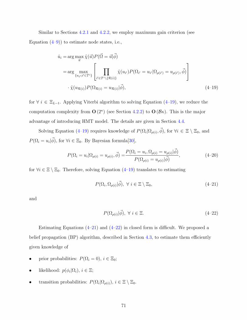
Similar to Sections 4.2.1 and 4.2.2, we employ maximum gain criterion (see

Equation (4–9)) to estimate node states, i.e.,

ui = arg max~u

χ(~u)P (~Ω = ~u|~φ)

= arg maxui′ ;i′∈T i

∏

i′∈T i\R(i)χ(ui′)P (Ωi′ = ui′|Ωρ(i′) = uρ(i′), ~φ)

· χ(uR(i))P (ΩR(i) = uR(i)|~φ), (4–19)

for ∀ i ∈ ΞL−1. Applying Viterbi algorithm to solving Equation (4–19), we reduce the

computation complexity from O (2κ) (see Section 4.2.2) to O (Bκ). This is the major

advantage of introducing HMT model. The details are given in Section 4.4.

Solving Equation (4–19) requires knowledge of P (Ωi|Ωρ(i), ~φ), for ∀i ∈ Ξ \ Ξ0, and

P (Ωi = ui|~φ), for ∀i ∈ Ξ0. By Bayesian formula[30],

P (Ωi = ui|Ωρ(i) = uρ(i), ~φ) =P (Ωi = ui, Ωρ(i) = uρ(i)|~φ)

P (Ωρ(i) = uρ(i)|~φ), (4–20)

for ∀i ∈ Ξ \ Ξ0. Therefore, solving Equation (4–19) translates to estimating

P (Ωi, Ωρ(i)|~φ), ∀ i ∈ Ξ \ Ξ0, (4–21)

and

P (Ωρ(i)|~φ), ∀ i ∈ Ξ. (4–22)

Estimating Equations (4–21) and (4–22) in closed form is difficult. We proposed a

belief propagation (BP) algorithm, described in Section 4.3, to estimate them efficiently

given knowledge of

• prior probabilities: P (Ωi = 0), i ∈ Ξ0;

• likelihood: p(φi|Ωi), i ∈ Ξ;

• transition probabilities: P (Ωi|Ωρ(i)), i ∈ Ξ \ Ξ0.

71

Usually it is difficult to estimate prior probabilities. In the paper, we simply assume

P (Ωi = 0) = P (Ωi = 1) = 12, i ∈ Ξ0. That is, states of root nodes are equally likely to

be normal or abnormal. Other parameters such as likelihood and transition probabilities

are estimated from training data. This is covered in Section 4.3. After that, classification

using maximum gain criterion is described in Section 4.4.

4.3 Estimation of HMT Parameters

In this section, we describe estimation of HMT parameters. It is organized as follows.

In Section 4.3.1, we describe estimation of likelihood p(φi|Ωi), i ∈ Ξ. Estimation of

transition probabilities P (Ωi|Ωρ(i)), i ∈ Ξ \ Ξ0 are presented in Section 4.3.2.

4.3.1 Likelihood Estimation

For the purpose of likelihood estimation, we collect two sets of training data.

• The set of features sampled in normal states, ~φ(k)0 ; k ∈ 1, . . . , K0, where K0 is

the number of normal samples and ~φ(k)0 =φ(k)

i,0 ; i ∈ Ξ, φ(k)i,0 denotes the kth feature

measured at node i;

• The set of features sampled in abnormal states, ~φ(k)1 ; k ∈ 1, . . . , K1, where K1 is

the number of abnormal samples and ~φ(k)1 =φ(k)

i,1 ; i ∈ Ξ, φ(k)i,1 denotes the kth feature

measured at node i.

Gaussian mixture model. In order to effectively estimate the likelihood, we assume

that the random variables/vectors, Φi|Ωi, i ∈ Ξ, follow a statistical distribution model.

Then, likelihood estimation translates to model parameters estimation. We establish the

statistical model in the following.

Because of its good properties, Gaussian (normal) distribution [30] is widely employed

in many applications. The pdf of a d-dimensional multivariate Gaussian distribution with

mean vector µ and variance matrix Σ is

N (x; µ, Σ)4=

1

(2π)d/2 |Σ|1/2exp

[−1

2(x− µ)tΣ−1(x− µ)

]. (4–23)

Figure 4-6 plots the pdf of the univariate Gaussian distribution N (x; 0, 1). It is observed

that Gaussian distribution is a unimodal distribution[30], i.e., its pdf only has one peak.

72

−4 −3 −2 −1 0 1 2 3 40

0.05

0.1

0.15

0.2

0.25

0.3

0.35

0.4

x

p(x)

N(0,1) distribution

Figure 4-6. Probability density function of the univariate Gaussian distribution N (x; 0, 1).

−100 0 100 200 300 400 500 6000

0.02

0.04

0.06

0.08

0.1

0.12Histogram

Figure 4-7. Histogram of the two-way matching features measured at a real networkduring network anomalies.

However, multiple peaks may exist in the empirical distribution of Φi|Ωi. For

example, Figure 4-7 shows the histogram of the two-way matching features measured

in a real network during DDoS attacks. It has two peaks. Hence, the unimodal Gaussian

distribution is not suitable. In the paper, we adopt the Gaussian mixture model (GMM)

to model the likelihood distribution.

73

The motivation of the GMM is the following. Suppose we first randomly pick a

number G from set 1, 2, . . . , G with probability P (G = g)=π(g), where

G∑g=1

π(g) = 1. (4–24)

Next, we generate a random variable X from a Gaussian distribution with pdf N (x; µ(g), Σ(g)).

Then the random variable X follows the G-state GMM, whose pdf is

pX(x) =G∑

g=1

N (x; µ(g), Σ(g)) π(g), (4–25)

where π(g), µ(g), and Σ(g) are known as prior probability, mean vector, and variance

matrix of the gth Gaussian distribution in the GMM, respectively. A G-state GMM has G

modes. Therefore, it is suitable to model distributions with multiple modes.

In the paper, we assume Φi|Ωi, i ∈ Ξ, follow G-state GMM. That is, the pdf of the

likelihood of node i is

p(φi|Ωi = u) =G∑

g=1

πi,u(g)N (φi; µi,u(g), Σi,u(g)) , (4–26)

for ∀i ∈ Ξ, ∀u ∈ 0, 1, where πi,u(g), µi,u(g), and Σi,u(g) are prior probability, mean

vector, and variance matrix of the gth Gaussian distribution at node i with state u,

respectively.

Next, we present schemes to estimate the GMM parameters.

GMM parameter estimation. Based on Equation (4–26), the likelihood estimation

translates to estimating GMM parameters πi,u(g), µi,u(g), and Σi,u(g) for ∀i ∈ Ξ,

∀u ∈ 0, 1, and ∀g ∈ 1, . . . , G, with constraint

G∑g=1

πi,u(g) = 1. (4–27)

Denote by πi,u(g), µi,u(g), and Σi,u(g) the estimates of πi,u(g), µi,u(g), and Σi,u(g),

respectively.

74

The most commonly used approach to estimate model parameters is the maximum-likelihood

(ML) method. Given the training features at node i with network state u, φ(1)i,u , . . . , φ

(Ku)i,u ,

the ML method chooses the parameters to maximize

Ku∏

k=1

p(φ(k)i,u |Ωi = u), (4–28)

where p(·|Ωi = u) is given in Equation (4–26). Unfortunately, Nechyba[32] showed

that ML method for G-state GMM with G > 1 has no closed form solution. In

addition, a G-state GMM has a 3G-dimensional continuous parameter space. Exhaustive

searching numerical solution for ML estimate in such a parameter space is computational

intractable.

1. Input: φ(k)i,u , k ∈ 1, . . . , Ku; π

(0)i,u (g), µ

(0)i,u(g), and Σ

(0)i,u(g), g ∈ 1, . . . , G.

2. Output: πi,u(g), µi,u(g), and Σi,u(g), g ∈ 1, . . . , G.3. j = 0.4. repeat

5. ϑ(j)i,u(g, φ)

4=

N(φ;µ

(j)i,u(g),Σ

(j)i,u(g)

)π

(j)i,u(g)

∑Gg=1N

(φ;µ

(j)i,u(g),Σ

(j)i,u(g)

)π

(j)i,u(g)

6. π(j+1)i,u (g) = 1

Ku

∑Ku

k=1 ϑ(j)i,u(g, φ

(k)i,u )

7. µ(j+1)i,u (g) =

∑Kuk=1 ϑ

(j)i,u(g,φ

(k)i,u)φ

(k)i,u∑Ku

k=1 ϑ(j)i,u(g,φ

(k)i,u)

8. Σ(j+1)i,u (g) =

∑Kuk=1 ϑ

(j)i,u(g,φ

(k)i,u)‖φ(k)

i,u−µ(j+1)i,u (g)‖2

∑Kuk=1 ϑ

(j)i,u(g,φ

(k)i,u)

9. j ← j + 110. until converge11. πi,u(g) = π

(j)i,u(g), µi,u(g) = µ

(j)i,u(g), Σi,u(g) = Σ

(j)i,u(g), ∀g ∈ 1, . . . , G.

Figure 4-8. The EM algorithm for estimating p(φi|Ωi = u), i ∈ Ξ, u ∈ 0, 1.

A practical solution to this issue is the expectation-maximization (EM) algorithm[29,

30]. Nechyba[32] derived EM algorithm for GMM in detail. Figure 4-8 illustrates the

algorithm.

The EM algorithm requires initial values for the parameters, as denoted by π(0)i,u (g),

µ(0)i,u(g), and Σ

(0)i,u(g) in Figure 4-8. At each iteration j, the EM algorithm uses parameters

estimated at iteration j − 1 to calculate new estimates. Although both EM and ML

75

methods scan the parameter space, EM works in a better way. It is proven that after each

iteration, EM algorithm guarantees to generate estimates of parameters which increase

Equation (4–28). As a result, EM algorithm converges much faster than numerical ML

method.

However, the disadvantage of EM algorithm is that it converges to a local maxima

rather than the global one. Specifically, initial values of parameters determine the local

maxima to which the EM algorithm converges. In practice, we have prior knowledge of

network features, which helps to choose initial values of parameters.

Till now, we present schemes to estimate likelihood of HMT. In next section, we

estimate transition probabilities.

4.3.2 Transition Probability Estimation

In this section, we estimate P (Ωi|Ωρ(i)), i ∈ Ξ \ Ξ0. Since closed form representation of

the transition probabilities is not available, we also estimate them in an iterative way.

Denote by ~φ(k); k ∈ 1, . . . , K the set of training features for transition probability

estimation, where ~φ(k) = φ(k)i ; i ∈ Ξ. Figs. 4-9 and 4-10 show the pseudo-code for

transition probability estimation. In next two sections, we explain the two figures.

Iteratively estimate transition probabilities. Figure 4-9 shows the pseudo-code

to estimate transition probabilities. The function TransProbEstimate takes three sets of

arguments:

1. likelihood estimated in Section 4.3.1, p(φi|Ωi); i ∈ Ξ;

2. training features, ~φ(k); k ∈ 1, . . . , K.It returns the estimate of transition probabilities, i.e.,

P (Ωi|Ωρ(i)), ∀ i ∈ Ξ \ Ξ0.

Before the iterations, we set the initial transition probabilities to be 12

at line 5 of

Figure 4-9. This is equivalent to assume normal state and abnormal state to be initially

76

1. function TransProbEstimate(. . .)2. Argument 1: likelihood, p(φi|Ωi); i ∈ Ξ.3. Argument 2: training data, ~φ(k); k ∈ 1, . . . , K.4. Return: transition probability estimate: P (Ωi = ui|Ωρ(i)), i ∈ Ξ \ Ξ0.5. P (0)(Ωi = u|Ωρ(i) = u′) = 1

2, for ∀ i ∈ Ξ \ Ξ0, ∀ u, u′ ∈ 0, 1.

6. j = 0.7. repeat8. for k ← 1 to K9.

P (j+1)(Ωρ(i)|~φ(k)), P (j+1)(Ωi, Ωρ(i)|~φ(k)); i ∈ Ξ \ Ξ0

=BP(

P (j)(Ωi|Ωρ(i)); i ∈ Ξ \ Ξ0

, p(φi|Ωi); i ∈ Ξ , ~φ(k)

)(4–29)

10. end for11. for ∀ i ∈ Ξ \ Ξ0

12.

P (j+1)(Ωi|Ωρ(i)) =1

K

K∑

k=1

P (j+1)(Ωi, Ωρ(i)|~φ(k))

P (j+1)(Ωρ(i)|~φ(k))

=1

K

K∑

k=1

P (j+1)(Ωi|Ωρ(i), ~φ(k)) (4–30)

13. end for14. j ← j + 115. until converge16. P (Ωi|Ωρ(i))=P (j)(Ωi|Ωρ(i)).

Figure 4-9. Iteratively estimate transition probabilities.

equally likely. Then, at each iteration, we update the estimate of transition probabilities

until it converges. The update procedure is the following.

First, we iterate the training feature set. For each feature, we use BP algorithm (see

Figure 4-10) to estimate the posterior probabilities given that feature. The details of the

BP algorithm is discussed in the next section.

Three sets of arguments are passed to the BP algorithm:estimate of transition probabilities obtained at the previous iteration,

P (j)(Ωi|Ωρ(i)); i ∈ Ξ \ Ξ0

;

1. likelihood, p(φi|Ωi); i ∈ Ξ, which is the argument passed to function TransProbEsti-mate;

77

1. function BP(. . .)2. Argument 1: transition probabilities,

P (Ωi|Ωρ(i)); i ∈ Ξ \ Ξ0

.

3. Argument 2: likelihood, p(φi|Ωi); i ∈ Ξ.4. Argument 3: training feature, ~φ.

5. Return: posterior probabilities,

P (Ωρ(i)|~φ), P (Ωi, Ωρ(i)|~φ); i ∈ Ξ \ Ξ0

.

6. Υi(0) = Υi(1) = 12, for ∀i ∈ Ξ0(i.e., roots).

7. υi(u) = p(φi|Ωi = u), for ∀i ∈ ΞL−1(i.e., leaves), ∀u ∈ 0, 1.8. Top-down pass, i.e., from root to leaf:9. for l ← 1, . . . , L− 1

10. for ∀ i ∈ Ξl,∀ u ∈ 0, 1, let11.

Υi(u) =∑

u′∈0,1P

(Ωi = u|Ωρ(i) = u′

)Υρ(i)(u

′)p(φρ(i)|uρ(i) = u′) (4–31)

12. end for13. end for14. Bottom-up pass, i.e., from leaf to root;15. for l ← L− 2, . . . , 016. for ∀ i ∈ Ξl, ∀ u ∈ 0, 1, let17.

υi(u) = p(φi|Ωi = u)∏

j∈ν(i)

∑

u′∈0,1P (Ωj = u′|Ωi = u) υj(u

′)

(4–32)

18. end for19. end for20.

P (Ωρ(i) = u|~φ) =Υi(u)υi(u)∑u′ Υi(u′)υi(u′)

(4–33)

21.

P (Ωi = u, Ωρ(i) = u′|~φ)

=υi(u)υρ(i)(u

′)P(Ωi = u|Ωρ(i) = u′

)Υρ(i)(u

′)

[∑

u′′ Υi(u′′)υi(u′′)][∑

u′′ P(Ωi = u′′|Ωρ(i) = u′

)υi(u′′)

] (4–34)

Figure 4-10. Belief propagation algorithm.

78

2. current training feature, ~φ(k).

It returns estimate of posterior probabilities

P (j+1)(Ωρ(i)|~φ(k)), P (j+1)(Ωi, Ωρ(i)|~φ(k)); i ∈ Ξ \ Ξ0

.

With the posterior probabilities obtained through BP algorithm, we update the

estimates of transition probabilities by Equation (4–30) for ∀ i ∈ Ξ \ Ξ0 and step to the

next iteration. When the estimates converge, iteration stops and Function TransProbEsti-

mate returns estimates obtained at the last iteration.

The validity of Equation (4–30) is shown in the following. For ∀ i ∈ Ξ \ Ξ0,

P (Ωi|Ωρ(i)) =

∫P (Ωi|Ωρ(i), ~Φ = ~φ)p(~φ)d~φ

=E~Φ

[P ((Ωi|Ωρ(i), ~Φ))

], (4–35)

where E [·] represents statistical expectation and the subscript stands for the random

variable over which expectation is taken. Because sample average is always the best

unbiased estimate of statistical expectation[30], we estimate

E~Φ

[P ((Ωi|Ωρ(i), ~Φ))

]

by

1

K

K∑

k=1

P (Ωi|Ωρ(i), ~φ(k)) =

1

K

K∑

k=1

P (Ωi, Ωρ(i)|~φ(k))

P (Ωρ(i)|~φ(k)). (4–36)

Combining Equations (4–35) and (4–36), we obtain Equation (4–30).

Next, we discuss the belief propagation algorithm, which is called by function

TransProbEstimate.

Belief propagation algorithm. The BP algorithm [33–35], also known as the

sum-product algorithm, e.g., [36–39], is an important method for computing approximate

marginal distributions. In this paper, we apply the BP algorithm to estimating posterior

probabilities (Figure 4-10).

79

Function BP takes three sets of arguments:

1. transition probabilities,P (Ωi|Ωρ(i)); i ∈ Ξ \ Ξ0

;

2. likelihood , p(φi|Ωi); i ∈ Ξ;

3. the training feature, ~φ,

and returns estimates of the posterior probabilities,

P (Ωρ(i)|~φ), P (Ωi, Ωρ(i)|~φ); i ∈ Ξ \ Ξ0

.

In Function BP(), we define two sets of transitory variables for convenience, i.e.,

Υi(u)4=p

(Ωi = u, ~φT\i

), (4–37)

υi(u)4=p

(~φTi|Ωi = u

), (4–38)

where u ∈ 0, 1, i ∈ Ξ.

Function BP() first initializes the variables Υi(u) for root nodes and υi(u) for leaves.

• When i ∈ Ξ0, i.e., root nodes, T\i = ∅, such that Υi(u) = P (Ωi = u). Hence, we letΥi(0) = 1

2and Υi(1) = 1

2for all root nodes i(see line 6 of Figure 4-10), because we

assume root nodes are equally likely to be in normal or abnormal state.

• When i ∈ ΞL−1, i.e., leaf nodes, ~φTi= ~φi, therefore υi(u) = p(φi|Ωi = u), u ∈ 0, 1

(see line 7 of Figure 4-10).

Then it propagates belief on the tree roots and leaves to other nodes in top-down pass

and bottom-up pass, respectively.

• During the top-down pass, Function BP iterates from root to leaf. At each level l,we update the transitory variables Υi(u) by Equation (4–31), which is proven inAppendix A.1. Note that, Υρ(i)(u

′) in Equation (4–31) is obtained in the previousiteration, i.e., iteration at level l − 1.

• During the bottom-up pass, Function BP iterates from leaf to root. at each levell, we update the transitory variables υi(u) by Equation (4–32), which is provenin Appendix A.2. Also note that, υj(u

′) is obtained in the previous iteration, i.e.,iteration at level l + 1.

80

Finally, we obtain the posterior probabilities by Equations (4–33) and (4–34). These

two equations are proven in Appendix A.3 and A.4, respectively. The estimated posterior

probabilities are used in Function TransProbEstimate to update estimates of transition

probabilities (see Figure 4-9).

Till now, we established the HMT model and described approaches to estimate

its model parameters from training data. Next, we present network anomaly detection

approaches using the fully determined HMT model.

4.4 Network Anomaly Detection Using HMT

In this section, we present the network anomaly detection using HMT model. This

is equivalent to a decoding problem in terms of pattern classification. That is, given an

observation sequence, i.e., extracted features ~φ = φi; i ∈ Ξ, and a HMT model defined by

• prior probabilities: P (Ωi), i ∈ Ξ0;

• likelihood: p(φi|Ωi), i ∈ Ξ;

• transition probabilities: P (Ωi|Ωρ(i)), i ∈ Ξ \ Ξ0,

we need to compute the “best” state combination ~Ω = Ωi; i ∈ Ξ. Here, the word

“best” is in terms of maximum gain criterion, as illustrated in Equation (4–19). We

rewrite the criterion in Equation (4–39),

ui = arg maxui′ ;i′∈T i

∏

i′∈T i\R(i)χ(ui′)P (Ωi′ = ui′|Ωρ(i′) = uρ(i′), ~φ)

· χ(uR(i))P(ΩR(i) = uR(i)|~φ

), (4–39)

for ∀ i ∈ Ξ. Function ViterbiDecodeHMT, as illustrated in Figure 4-11, shows the

pseudo-code for the classification algorithm.

Function ViterbiDecodeHMT takes three arguments. The first two arguments, the

transition probabilities and the likelihood, are estimated during training phase. The

last one is the extracted features, based on which we perform anomaly detection. It

returns the estimates of node states. Among them, we are only interested in states of leaf

81

nodes, which represent whether an edge router is in abnormal state. Next, we explain the

algorithm in detail.

1. function ViterbiDecodeHMT(. . .)2. Argument 1: transition probabilities,

P (Ωi|Ωρ(i)); i ∈ Ξ \ Ξ0

.

3. Argument 2: likelihood, p(φi|Ωi); i ∈ Ξ.4. Argument 3: feature, ~φ.5. Return: estimated node states, ui; i ∈ Ξ.6.

P (Ωρ(i)|~φ), P (Ωi, Ωρ(i)|~φ); i ∈ Ξ \ Ξ0

=BP(

P (Ωi|Ωρ(i)); i ∈ Ξ \ Ξ0

, p(φi|Ωi); i ∈ Ξ , ~φ

)(4–40)

7.

P(Ωi|Ωρ(i), ~φ

)=

P(Ωi, Ωρ(i)|~φ

)

P(Ωρ(i)|~φ

) (4–41)

8. for ∀ i ∈ Ξ0

9. ui = arg maxuiP (Ωi = ui|~φ)

10. end for11. for l ← 1, . . . , L− 1, for ∀ i ∈ Ξl

12.

ui = arg maxui

χ(ui)P(Ωi = ui|Ωρ(i)=uρ(i),~φ

)·

∏

i′∈T ρ(i)\R(i)

χ(ui′)P(Ωi′ = ui′|Ωρ(i′) = uρ(i′), ~φ

) χ(uR(i))P

(ΩR(i) = uR(i)|~φ

)

(4–42)

13. end for

Figure 4-11. Viterbi algorithm for HMT decoding.

By Bayesian formula, the terms in Equation (4–39) can be computed by

P(Ωi′ = ui′|Ωρ(i′) = uρ(i′), ~φ

)=

P(Ωi′ = ui′ , Ωρ(i′) = uρ(i′)|~φ

)

P(Ωρ(i′) = uρ(i′)|~φ

) , (4–43)

82

where i′ ∈ Ξ\Ξ0. Therefore, it also requires to calculate posterior probabilities. We employ

BP algorithm (see Equations (4–40) and (4–41) in Figure 4-11) to solve Equation (4–43) in

a way similar to HMT transition probability estimation(see Figure 4-10).

Obtaining solutions to Equation (4–43) for all nodes, we can solve Equation (4–39). A

brute force solution to Equation (4–39) is to exhaustively compute

∏

i′∈T i\R(i)χ(ui′)P (Ωi′ = ui′|Ωρ(i′) = uρ(i′), ~φ)

χ(uR(i))P

(ΩR(i) = uR(i)|~φ

), (4–44)

for ∀ i ∈ Ξ \ Ξ0, ∀ ~u ∈ Space of ~Ω and select the “best” one. A HMT with L levels

modeling an AS with κ edge routers has

BdlogB κe1− B−L

1− B−1

nodes, each of which has two states, normal and abnormal. Then the ~Ω space has

2BdlogB κe 1−B−L

1−B−1

possible values. The computation complexity of the brute force method is

O(2BdlogB κe)

,

even worse than the dependent model (see Figure 4-4), whose complexity is

O (2κ) .

In this paper, we applied Viterbi algorithm [40–42] to solving Equation (4–39) in an

iterative manner, reducing the computational complexity to O (Bκ).

The motivation of Viterbi algorithm is the following. It iterates from top level of a

HMT to bottom level. At each iteration, it estimates the node states in that level in a way

that, when combined with states estimated in upper levels, “best” explains the observed

features. That is, at each iteration, Viterbi algorithm always selects the local maxima.

83

Although it does not guarantee to find the global optimal solution to Equation (4–39),

Viterbi algorithm is efficient and has good performance empirically.

The computation complexity of Viterbi algorithm is O (Bκ), much better than

the dependent model, as illustrated in Figure 4-4, whose complexity is O (2κ). The

performance improvement results from the fact that Viterbi algorithm does not exhaustively

test all possible node state combinations. Instead, we decompose the decoding problem

into multiple stages, each of which decodes node states at one level in HMT. At level l, we

estimate node states of level l, i.e., Ωi; i ∈ Ξl, based on results obtained during previous

stages, i.e. Ωi; i ∈ Ξ0, . . . , Ξl−1. In such a procedure, each node is only accessed for

twice. Hence the complexity is linear to the number of nodes, which is

BdlogB κe1− B−L

1− B−1< Bκ

1− B−L

1− B−1≈ Bκ.

Till now, we described the HMT model, including its parameter training and

classification approaches. Next, we show the simulation results of applying the HMT

model to network anomaly detection.

4.5 Simulation Results

In this section, we evaluate the performance of the proposed schemes through

simulation.

4.5.1 Experiment Setting

In our study, we develop a testbed to 1) extract various feature information, and 2)

analyze feature data by our machine learning algorithm and CUSUM algorithms. Next,

we describe the setting for networks, traffic traces, and feature extraction used in our

experiments.

Network.

In our experiment, we assume that the ISP network consists of a core AS, a victim

subnet, and 16 edge routers that connect to 16 subnets, as illustrated in Figure 4-12. At

each edge router, two monitors are placed to measure the inbound and outbound traffic

84

Figure 4-12. Experiment Network

between a subnet and the victim network, respectively. For convenience, we denote a link

as the route between an edge router and the victim subnet.

Traffic. A link may carry normal traffic (called background traffic) or abnormal

traffic. For the background traffic, we use the same data set as in Section 3.7.2[27]. Since

we do not have real data traces obtained from 16 different links, we use the real traffic

trace measured on one link (between the Internet and Auckland University) in 16 different

days to create traffic traces for 16 different links.

For the abnormal traffic, we randomly generate TCP SYN flood attacks into the

background trace. Specifically, we generate several attack scenarios. For each scenario,

we randomly select the abnormal links and attack durations. Attack traffic on each link

is generated in the same way as in Section 3.7.2. That is, we randomly insert TCP SYN

packets with random source IP addresses into the background traffic of that link. The

average packet rate of TCP SYN attack traffic on each selected link is 1% of the total

packet rate on the link. For each attack scenario, attacks on each of the selected links are

launched during almost the same period to simulate the synchronized DDoS attacks. Since

the attack traffic on each link is low (just 1%), we effectively simulate low volume attack

traffic.

85

Features.

To detect distributed TCP SYN attacks, we use the two-way matching features

described in Chapter 3, i.e., the number of unmatched inbound SYN packets in one

time slot. The parameter setting of two-way matching features extraction is same as in

Section 3.7.2. For convenience, we summarize the parameters in Table 4-3.

Table 4-3: Parameter setting of feature extraction for network anomaly detectionNotation DescriptionR 2480η 0.1%K 8w 8γ 10 secondsMv 215 bits

For comparison purpose, we also measure the number of SYN packets and SYN/FIN

ratio[11] in a slot.

4.5.2 Performance Comparison

Table 4-4: Performance of different schemes.Feature Detection algorithm Detection probability False alarm probabilitySYN/FIN ratio CUSUM 0.174 0.129SYN CUSUM 0.52 0.129SYN Machine learning 0.656 0.123Unmatched SYN CUSUM 0.690 0.130Unmatched SYN Machine learning 0.973 0.115

Table 4-4 compares the performance of different schemes, where the benchmark is

the scheme in [11], i.e., the CUSUM scheme with SYN/FIN ratio as the feature; for the

benchmark scheme, we use the same parameter setting as that in [11]; we compare the

benchmark with CUSUM and our machine learning algorithm under different features.

To make fair comparison, we make the false alarm probability of each scheme almost

the same and compare the detection probability. From Table 4-4, it can be seen that,

the benchmark scheme (‘SYN/FIN ratio’+CUSUM) performs very poorly in detecting

low volume DDoS attacks. In contrast, a CUSUM algorithm with the number of SYN

86

packets or the number of unmatched SYN packets as the feature can achieve much higher

detection probability. More importantly, our machine learning algorithm can significantly

outperform CUSUM, given the same feature data, no matter whether the feature is the

number of SYN packets or the number of unmatched SYN packets.

0

0.2

0.4

0.6

0.8

1

0 0.2 0.4 0.6 0.8 1

Det

ectio

n P

roba

bilit

y

False Alarm Probability

Threshold (SYN)Machine Learning (SYN)

Threshold (UM-SYN)Machine Learning (UM-SYN)

Figure 4-13. Performance of threshold-based and machine learning algorithms withdifferent feature data

Figure 4-13 compares the ROC curve of the threshold-based scheme described in

Section 4.1.2 and our machine learning algorithm under two different features, i.e., the

number of SYN packets (denoted by ‘SYN’) and the number of unmatched SYN packets

(denoted by ‘UM-SYN’). We observe that, for the same detection algorithm, using the

number of unmatched SYN packets can significantly improve the ROC performance,

compared to using the number of SYN packets. In other words, given the same false alarm

probability, the detection probability is much higher when using the number of unmatched

SYN as feature.

Another important observation from Figure 4-13 is that given the same feature data,

our machine learning algorithm can (significantly) improve the ROC, compared to the

threshold-based scheme; e.g., for the same false alarm probability of 0.05, our machine

learning algorithm achieves a detection probability of 0.93, while the threshold-based

scheme only achieves a detection probability of 0.72. This is due to the fact that our

87

machine learning algorithm exploits the spatial correlation among traffic on multiple links,

while the threshold-based scheme only uses the traffic on one link.

0

0.2

0.4

0.6

0.8

1

0.0001 0.001 0.01 0.1 1

Det

ectio

n P

roba

bilit

y

False Alarm Probability

Single CUSUMDual CUSUM

ThresholdMachine Learning

Figure 4-14. Performance of four detection algorithms

In Figure 4-14, we compare the ROC performance of four detection algorithms (the

threshold-based, the single-CUSUM, the dual-CUSUM described in Section 4.1.3, and our

machine learning algorithm) under the same feature, i.e., the number of unmatched SYN

packets. For the single-CUSUM and the dual-CUSUM algorithm, the detection delay D is

chosen from 1 to 10 slots and the parameter ai of link i is determined by

ai = (Dattack − Dnormal)× i

17, ∀ 1 ≤ i ≤ 16,

where Dattack and Dnormal are the average number of unmatched inbound SYN packets in

attack and normal conditions, respectively.

The ROC performance (Figure 4-14) of our machine learning algorithm is the

best among all the algorithms. We also see that the dual-CUSUM out-performs the

simple threshold-based algorithm and the single-CUSUM algorithm has the worst ROC

performance.

4.5.3 Discussion

We would like to point out that, besides detecting network anomalies with low

volume traffic, our machine learning algorithm is also able to detect high volume anomaly,

88

the results of which are not shown here due to the space limit. The machine learning

algorithm is shown to be robust under realistic time-varying traffic patterns such as

the Auckland data traffic [27]. We tested our machine learning algorithms for a large

IP address space, i.e., the IP address space can be the whole IP address space for the

Internet.

4.6 Summary

In this chapter, we propose a novel machine learning detection algorithm, based on

Bayesian decision theory and hidden Markov tree model. The key idea of our algorithm is

to exploit spatial correlation of network anomalies. Our detection scheme has the following

nice properties:

• In addition to detecting network anomalies having high-data-rate on a link, ourscheme is also capable of accurately detecting attacks having low-data-rate onmultiple links. This is due to exploitation of spatial correlation of network anomalies.

• Our scheme is robust against time-varying traffic patterns, owing to powerful machinelearning techniques.

• Our scheme can be deployed in large-scale high-speed networks, thanks to use ofBloom filter array to efficiently extract features.

With the proposed techniques, our scheme can effectively detect network anomalies

without modifying existing IP forwarding mechanisms at routers. Our simulation results

show that the proposed framework can detect DDoS attacks even if the volume of attack

traffic on each link is extremely small (i.e., 1%). Especially, for the same false alarm

probability, our scheme has a detection probability of 0.97, whereas the existing scheme

has a detection probability of 0.17, which demonstrates the superior performance of our

scheme.

89

CHAPTER 5NETWORK CENTRIC TRAFFIC CLASSIFICATION: AN OVERVIEW

In Chapters 5 and 6, we focus on the second part of our research, i.e., network centric

traffic classification. This chapter motivates the significance and points out the challenges

of this issue, and shows weakness of existing solutions.

5.1 Introduction

The Telecom business is rapidly changing. Commoditized below profitable levels,

traditional circuit-switched voice service just is not lucrative anymore. Since 2000, the

drop in traditional voice revenue has prompted the large telcos to explore new business

opportunities. Services over IP (SoIP) have been identified as the new streams to continue

growing. Among all the SoIP, VoIP and IPTV are the most attractive ones as they are

trusted to represent the largest source of profits as consumer interest in online voice and

video services increases, and as broadband deployments proliferate. According to Point

Topic research firm, there were 209.3 million global broadband users at the end of 2005,

up to 56.2 million from 153.3 million lines on 31 December 2004. As a consequence, VoIP

and IPTV user population is expected to grow dramatically in the next few months. For

example, France Telecom released on July 2006 that the number of its VoIP users grew

80% in the last 6 months to a total of 1.73 million as of June 30th, 2006. Same for IPTV

users expected to grow from 300,000 today to 5 million in the next 2 years.

But to tap the potential profits that SoIP offers, the infrastructure of carrier networks

needs to evolve. Next-generation Networks (NGN) feature the convergence of access

technologies (wireline, wireless, cellular), information services (voice, broadband, data,

content), and devices (consumer electronics, traditional telecom equipment). Such

multi-layered convergence promises reduced costs, greater workforce and consumer

mobility, and exciting new business models. However, the trend toward convergence

creates a strong need for fair methods of efficiently and accurately managing and tracking

the delivery of IP services. As carriers transition to becoming service providers, they begin

90

to sell and deliver IP services to their customers. Unfortunately the emergence of a bloom

of new zero-day voice and video applications over IP, like Skype, Google Talk (Gtalk),

MSN, etc, the proliferation of new peer-to-peer protocols that now allow the usage of voice

and video among other applications, and the continuing growth of the usage of encryption

techniques to protect data confidentiality, lead to tremendous revenue leakage for ISPs due

to their inefficiency in detecting these new applications and thus lack of proper actions.

The result from unmanaged commercial traffic adds up to loss of hundreds of millions of

dollars annually and poses a solid road block to the profitability of ISPs’ VoIP and IPTV

services.

As a consequence, it is imperative for ISPs to identify robust solutions for detecting

voice and video over IP data-streams. The most common approach for identifying

applications on an IP network is to associate the observed traffic with an application

based on TCP or UDP port numbers [43, 44]. In principle the TCP and UDP server

port numbers can be used to identify the higher layer application, by simply identifying

the server port and mapping this port to an application using the Internet Assigned

Numbers Authority (IANA) list of registered ports [45]. However, port-based application

classification has limitations due to the emergence of new applications that no longer

use fixed, predictable port numbers. For example, non-privileged users often have to use

ports above 1024 to circumvent operating system access control restrictions; or common

applications like FTP allows the negotiation of unknown and unpredictable server ports to

be used for the data transfer; or proprietary applications may deliberately try to hide their

existence or bypass port-based filters by using standard ports. For example, server port 80

is being used by a large variety of non-web applications to circumvent firewalls which do

not filter port-80 traffic; others (e.g., Skype) tend to use dynamic ports.

A more reliable technique involves stateful reconstruction of session and application

information from packet contents [46–48]. Although this avoids reliance on fixed port

numbers, it imposes significant complexity and processing load on the classification device,

91

which must be kept powerful enough to perform concurrent analysis of a large number

of flows while applying techniques to search very complex protocol signatures that might

require processing of a large chunk of packet payload. The proliferation of proprietary

protocols, coupled with the growing trend in the usage of encryption techniques to ensure

data confidentiality, makes this approach infeasible. For example, Skype does not run on

any standard port, but randomly selects ports for its communication and use either the

TCP, or UDP or both for the data transfer. Furthermore, its use of a 256-bit encryption

algorithm and no visibility into neither the algorithm nor its keys makes its detection

even harder. All the above makes the general problem of the detection of VoIP and video

data-streams over IP challenging and yet it is of huge business interest.

A new emerging tendency in the research community to approach this problem is

to rely on pattern classification techniques. This new family of techniques formulate

the application detection problem as a statistical problem that develop discriminating

criteria based on statistical observations and distributions of various flow properties in the

packet traces. A few papers [49, 50] have taken this statistical approach to classify traffic

into p2p, multimedia streaming, interactive application, and bulk transfer application.

Unfortunately, although these papers addressed the problem of distinguishing multimedia

traffic from other applications, they have not addressed the problem of distinguishing

voice traffic from video traffic. One problem is to separate streaming traffic from other

applications, and a different problem is to detect and correctly classify voice and video and

clearly separate the two applications from each other. In the extreme case, voice and/or

video data streams might even be bundled together in the same exact flow with other

applications. These problems are common for many applications like Skype, Gtalk and

MSN that allow users to mix voice and/or video streams with chat and/or file transfer

traffic in the same exact 5-tuple flow, defined as ¡source IP address, destination IP address,

source port, destination port, and protocol number¿. In such cases, one flow may carry

92

traffic from multiple types of applications (such as voice, video, chat, and file transfer),

referred to as hybrid flow in the remainder of this paper.

Our research focuses on detecting and classifying voice and video traffic and further

deal with its more general formulation that considers the presence of hybrid flows.

Based on the intuitions that voice and video data streams show strong regularities in

the inter-arrival times of packets within the flow and the associated packet sizes when

combined together in one single stochastic process and analyzed in the frequency domain,

we propose a system, called VOVClassifier , for voice and video traffic classification.

VOVClassifier is an automated self-learning system that is composed of four

major modules operating in cascade. The system first is trained with voice and video

data streams and afterwards enters the classification phase. During the training

period, all packets belonging to the same flow are extracted and used to generate a

stochastic model that captures the features of interest. Then all flows are processed in

the frequency domain using Power Spectral Density (PSD) analysis in order to extract a

high-dimensional space of frequencies that carry the majority of energy of the signal. All

features extracted from each flow are grouped into a “feature vector”. Due to the wide

usage of different codecs for voice and video, we propose a second module that clusters the

feature vectors into several groups using Subspace Decomposition (SD) and then identifies

its subspace structure, e.g. bases of the subspace, using Principal Component Analysis

(PCA). These two steps are applied to all flows during the training period and produce

low-dimensional spaces, referred in the paper as voice subspace and video subspace.

After training, all flows are processed by the PSD module and the associated feature

vector is compared with the voice and video spaces obtained during training. The space at

minimum normalized distance from the feature vector is selected as candidate and chosen

if and only if its distance is below a specific predetermined threshold.

We applied VOVClassifier to real packet traces collected into two different network

scenarios. Results demonstrate the effectiveness and robustness of our approach, able to

93

achieve 100% detection rate of both voice and video in the case of single-typed flow, e.g.

one application per 5-tuple, and 98.6% and 94.8% respectively for voice and video when

dealing with the more complex scenario of hybrid flows, e.g. voice, video and file transfer

bundled together in the same 5-tuple flow.

The rest of the chapter is organized as follows. In Section 5.2, we introduce the

related work in the area of pattern classification methodologies. Section 5.3 describes

the weaknesses of metrics previously used by other works when applied in our context

and highlights the new traffic features that constitute the foundation of our approach.

Section 5.4 summarizes this chapter.

5.2 Related Work

Existing work on traffic classification uses discriminating criteria such as the packet

size distribution per flow, the inter-arrival times between packets within the same flow

and other statistics captured across multiple flows. For example, in Ref. [49], the authors

proposed the combination of average packet size within a flow and the inter-arrival

variability metric, e.g. defined as the ratio of the variance to the average inter-arrival

times of packets within a flow, as a powerful metric to define fairly distinct boundaries for

three groups of applications: (i) bulk data transfer like FTP, (ii) interactive like HTTP,

and (iii)streaming like voice, video, gaming, etc. Several classification techniques, like

nearest-neighbor and K-nearest-neighbor, were then tested using the above traffic features.

Although this preliminary study has proved that the approach of pattern classification has

great potential for a proper application classification, it proves that much more work still

remains, e.g. exploiting other alternative for traffic features and classification techniques.

Moreover, although the features extracted are simple and feasible to be implemented

on-the-fly, the learning algorithm is complex and the outcome boundaries among the three

families of applications are heavily non-linear and time-dependent.

Similar to Ref. [49], Karagiannis et al.[50] proposed a novel approach, called BLINC,

that exploits network-related properties and characteristics. The novelty of this approach

94

resides in twofold. First, the authors shift the focus from classifying individual flows to

associating Internet hosts with applications, and then classifying their flows accordingly.

Second, BLINC follows a different philosophy from previous methods attempting to

capture the inherent behavior of a host at three levels: (i) social level, e.g. how each host

interacts with other hosts, (ii) functional level, e.g. role played by each host in the network

as a provider of an application or a consumer of the application, and finally (iii) the

application level, e.g. ports used by each host during its communication with other hosts.

Although the approach proposed in [50] is interesting from a conceptual perspective and

proved to perform reasonably well for a variety of different applications, it is still prone

to large estimation errors for streaming applications. Moreover, its high complexity and

large memory consumption remains an open issue for high-speed application classification.

Other papers using pattern classification appeared lately in literature but more focused

on specific application detection like Peer-to-Peer [46] and chat [51]. More importantly, to

the best of our knowledge, none of the existing work has been able to separate voice traffic

from video traffic or to indicate the presence of voice traffic or video traffic in a hybrid

flow that contains traffic from both voice/video and other applications such as file transfer.

5.3 Intuitions Behind a Proper Detection of Voice and Video Streams

Generally speaking, the problem of voice and video detection can be formulated as

a complex pattern classification problem that has to deal with curse of dimensionality,

e.g. discrimination of voice and video data streams when dealing with hidden traffic

patterns and too many interrelated features. A critical step toward the solution is to

identify traffic features that correctly represent the characteristics of the data streams of

interest and uniquely isolate them from other applications. In order to achieve this, in this

section we start by showing how simple metrics presented in the past are not applicable

in our context and we conclude with some observations that constitute the essence of

our approach. In Figure 5-1 we show the results obtained when using the combination

of average packet size and the inter-arrival variability metric proposed by Roughan et

95

al. [49]. Although this metric performed very well in separating streaming, file transfer,

transactional and interactive applications, it performs poorly when used to further

separate applications within the same family, as voice, video or voice and video mixed

with other applications like file transfer, e.g. hybrid flows. Figure 5-1 clearly highlights the

complete absence of any distinct boundary and heavy overlapping between voice and video

traffic. The reasons why the pair (average packet size, inter-arrival variability metric)

cannot separate video from voice are as below. First, the packet size for video/voice is

controlled by the packetization strategy of the video/voice application designer [52]; hence,

a video application may produce similar average packet size to that for voice (Figure 5-1).

Second, random end-to-end delay in the Internet causes large variations in the inter-arrival

variability metric for different video/voice flows.

0 2 4 6 8 10 120

500

1000

1500

Inter−Arrival Variability Metric

Ave

rage

Pac

ket S

ize

(Byt

es)

audiofilefileaudiofilevideovideo

Figure 5-1. Average packet size versus inter-arrival variability metric for 5 applications:voice, video, file transfer, mix of file transfer with voice and video.

Table 5-1: Commonly used speech codec and their specificationsStandard Codec Method Inter-Packet Delay (ms)G.711[53] PCM .125G.726[54] ADPCM .125G.728[55] LD-CELP .625G.729[56] CS-ACELP 10G.729A[56] CS-ACELP 10G.723.1[57] MP-MLQ 30G.723.1[57] ACELP 30

96

In order to overcome the above problem, in this section we exploit different metrics

that might have great potential to serve our purpose: strong regularities of inter-arrival

times between packets within the same flow and packet sizes residing in voice and video

data streams. Specifically, we consider four types of metrics, i.e.,

1. packet inter-arrival time and packet size in time domain;

2. packet inter-arrival time in frequency domain;

3. packet size in frequency domain;

4. combining packet inter-arrival time and packet size in frequency domain.

These metrics are discussed later.

0 0.01 0.02 0.03 0.04 0.05 0.060

0.05

0.1

0.15

0.2

0.25

IAT (seconds)

pdf

AUDIOVIDEO

Figure 5-2. Inter-arrival time distribution for voice and video traffic

5.3.1 Packet Inter-Arrival Time and Packet Size in Time Domain

The intuitions behind such metrics reside in the observation that any protocol used

for voice and video applications specifies a constant time between two consecutive packets

at the transmitter side, also known as Inter-Packet Delay (IPD).For example, Table 5-1

lists some speech codec standards and the associated IPDs that are required for a correct

implementation of those protocols. Packets leaving the transmitter might traverse a

large number of links in the Internet before reaching the proper destination. Along this

97

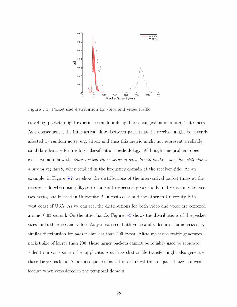
0 100 200 300 400 500 600 7000

0.01

0.02

0.03

0.04

0.05

0.06

0.07

Packet Size (Bytes)

pdf

AUDIOVIDEO

Figure 5-3. Packet size distribution for voice and video traffic

traveling, packets might experience random delay due to congestion at routers’ interfaces.

As a consequence, the inter-arrival times between packets at the receiver might be severely

affected by random noise, e.g. jitter, and thus this metric might not represent a reliable

candidate feature for a robust classification methodology. Although this problem does

exist, we note how the inter-arrival times between packets within the same flow still shows

a strong regularity when studied in the frequency domain at the receiver side. As an

example, in Figure 5-2, we show the distributions of the inter-arrival packet times at the

receiver side when using Skype to transmit respectively voice only and video only between

two hosts, one located in University A in east coast and the other in University B in

west coast of USA. As we can see, the distributions for both video and voice are centered

around 0.03 second. On the other hands, Figure 5-3 shows the distributions of the packet

sizes for both voice and video. As you can see, both voice and video are characterized by

similar distribution for packet size less than 200 bytes. Although video traffic generates

packet size of larger than 200, these larger packets cannot be reliably used to separate

video from voice since other applications such as chat or file transfer might also generate

these larger packets. As a consequence, packet inter-arrival time or packet size is a weak

feature when considered in the temporal domain.

98

5.3.2 Packet Inter-Arrival Time in Frequency Domain

We show how the same feature becomes a key reliable feature when observed in

the frequency domain. In this new domain, we are interested whether it does exist any

frequency component, e.g. inter-arrival time, that captures the majority of the energy of

this stochastic process at the receiver side. We exploit the above by computing the power

spectral density (PSD) analysis of the packet inter-arrival time process of two traces, each

of which is of length 10 second, in Figures 5-4 and 5-5 respectively for voice and video. We

can see that some regularity for both voice and video exist for different traces, although

the regularity is not quite strong. This result holds true for all experiments conducted

when transmitting Skype voice and video packets over the Internet from University A to

University B.

0 0.2 0.4 0.6 0.8 1−70

−60

−50

−40

−30

−20

−10

0

Normalized Frequency (×π rad/sample)

Pow

er S

pect

ral D

ensi

ty (

dB)

Trace 1Trace 2

Figure 5-4. Power spectral density of two sequences/traces of time-varying inter-arrivaltimes for voice traffic

5.3.3 Packet Size in Frequency Domain

Somewhat stronger regularity is visible for voice and video packet sizes. Indeed,

most video coding schemes use two types of frames[58], i.e., Intra frames (I-frame)

and Predicted frames (P-frame). An I-frame is a frame coded without reference to any

frame except itself. It serves as the starting point for a decoder to reconstruct the video

stream. A P-frame may contain both image data and motion vector displacements

99

0 0.2 0.4 0.6 0.8 1−45

−40

−35

−30

−25

−20

−15

−10

−5

0

Normalized Frequency (×π rad/sample)

Pow

er S

pect

ral D

ensi

ty (

dB)

Trace 1Trace 2

Figure 5-5. Power spectral density of two sequences of time-varying inter-arrival times forvideo traffic

and/or combinations of the two. Its decoding needs reference to previously decoded

frames. Packets containing I-frames are larger than those containing P-frames. Usually,

the number of P-frames between two consecutive I-frames is constant. Hence, one can

observe a strong periodic variation of packet size due to the interleaving of I-frames and

P-frames composing video data streams. Voice streams have similar phenomenon if Linear

Prediction Coding (LPC), e.g., code excited linear prediction (CELP) voice coder, is

employed. As an example, Figs. 5-6 and 5-7 show the power spectral density of voice and

video packet sizes, respectively.

5.3.4 Combining Packet Inter-Arrival Time and Packet Size in FrequencyDomain

Figs 5-8 and 5-9 show how the regularities hidden in voice and video data streams

can be amplified when combining the two features together in one single stochastic process

that will be described later in the paper. Note how the two important frequencies are

amplified and clearly visible in the PSD plots. The reason why there is a peak in the

PSD for voice (see Figure 5-8) is that voice applications usually produce close-to-constant

packet rate due to constant inter-packet delay of the widely used speech codecs listed

in Table 5-1; e.g., the peak of 33 Hz in Figure 5-8 corresponds to 30 ms inter-packet

100

0 0.2 0.4 0.6 0.8 110

20

30

40

50

60

70

80

Normalized Frequency (×π rad/sample)

Pow

er S

pect

ral D

ensi

ty (

dB)

Trace 1Trace 2

Figure 5-6. Power spectral density of two sequences of discrete-time packet sizes for voicetraffic

0 0.2 0.4 0.6 0.8 130

35

40

45

50

55

60

65

70

75

80

Normalized Frequency (×π rad/sample)

Pow

er S

pect

ral D

ensi

ty (

dB)

Trace 1Trace 2

Figure 5-7. Power spectral density of two sequences of discrete-time packet sizes for videotraffic

delay. Compared to voice, video applications have a flatter PSD. The reason is as below.

The number of bits in an I-frame of video depends on the texture of the image (e.g.,

the I-frame of a blackboard image produces much less bits than that of a complicated

flower image), resulting in a large range in the number of packets in an I-frame, e.g., from

1 packet to a few hundred packets produced by an I-frame. The frame rate is usually

constant (e.g., 30 frames/s is a standard rate in USA), i.e., a frame will be generated every

101

33 seconds for 30 frames/s; hence, the inter-arrival time between two packets in an I-frame

may span a large range, resulting in a flat PSD.

0 10 20 30 40 50−5

0

5

10

15

20

25

30

35

40

45

Frequency (Hz)

Pow

er S

pect

ral D

ensi

ty (

dB)

Trace 1Trace 2

Figure 5-8. Power spectral density of two sequences of continuous-time packet sizes forvoice traffic

0 100 200 300 400 50012

14

16

18

20

22

24

26

28

30

Frequency (Hz)

Pow

er S

pect

ral D

ensi

ty (

dB)

Trace 1Trace 2

Figure 5-9. Power spectral density of two sequences of continuous-time packet sizes forvideo traffic

5.4 Summary

In this chapter, we motivated the importance and presented challenges faced by

network traffic classification, specifically, detecting and classifying voice and video traffic.

102

Nowadays, VoIP and IPTV become increasingly popular and represent the largest

source of profits as consumer interest in online voice and video services increases, and

as broadband deployments proliferate. In order to tap the potential profits that VoIP

and IPTV offer, carrier networks have to efficiently and accurately manage and track the

delivery of IP services. Yet, the emergence of a bloom of new zero-day voice and video

applications such as Skype, Gtalk, and MSN poses tremendous challenges for ISPs. The

traditional approach of using port numbers to classify traffic is infeasible due to the usage

of dynamic port number. The proliferation of proprietary protocols, coupled with the

growing trend in the usage of encryption techniques to ensure data confidentiality, makes

application-level analysis infeasible. We also proposed a novel problem that multiple

sessions reuse the same transport layer connection. To our best knowledge, this problem

has never been considered in existing literatures.

We showed that existing technologies (Section 5.2) are not able to accurately

distinguish between voice and video flows. By analyzing the properties of voice and

video data streams, our intuition is to exploit the strong regularities residing in packet

inter-arrival times and the associated packet sizes. In this chapter, we analyze four types

of metrics that exploit the regularities,

1. packet inter-arrival time and packet size in time domain;

2. packet inter-arrival time in frequency domain;

3. packet size in frequency domain;

4. combining packet inter-arrival time and packet size in frequency domain.

By analyzing properties and illustrating figures of the four types of metrics, we show

that combining packet inter-arrival time and packet size in one single stochastic process

generates distinctive feature to classify voice and video streams.

103

CHAPTER 6NETWORK CENTRIC TRAFFIC CLASSIFICATION SYSTEM

6.1 System Architecture

Figure 6-1. VOVClassifier System Architecture

We first present the overall architecture of our system (VOVClassifier , Figure 6-1),

and provide a high-level description of the functionalities of each of its modules. Generally

speaking, VOVClassifier is an automated learning system that uses packet headers from

raw packets collected off the wire, organize them into transport network flows and process

them in realtime to search for voice and video applications. VOVClassifier first trains voice

and video data streams separately before being used in realtime for classification. During

the training phase, VOVClassifier extracts feature vectors, which is a summary (also

known as a statistic) of raw traffic bit stream, and maintain their statistics in memory.

During the online classification phase, a classifier makes decision by measuring similarity

metrics between the feature vector extracted from on-the-fly network traffic and the

feature vectors extracted from training data. Flows with high values of similarity metric

with the voice (or video) features are classified as voice(or video); data streams with low

values of similarity with voice/video are classified as other applications.

In general, VOVClassifier is composed of four major modules that operate in cascade:

(i) Flow Summary Generator (FSG),(ii) Feature Extractor (FE) via Power Spectral

104

Density analysis, (iii) Voice/video-Subspace Generator (SG) and (iv) Voice/video-

CLassifier (CL).

Next, we briefly summarize the functionalities of each component.

6.1.1 Flow Summary Generator (FSG)

All packets collected off-the-wire are processed by the Flow Summary Generator

module, that reorders packets by removing any duplicated packet, and organizes them into

network transport flows according to their 5-tuple, e.g., source IP, destination IP, source

Port, destination Port and transport protocol. In Section 5.3 we have shown as voice and

video data streams that are characterized by packets that are very small in size. As a

consequence, this module filters out all packets whose size is smaller than a pre-specified

threshold θP . The processed flow is then internally described in terms of packet sizes and

inter-arrival times between packets within any generic flow FS.

FS = 〈Pi,Ai〉 ; i = 1, . . . , I , (6–1)

where Pi and Ai denote the packet size and relative packet arrival time of the ith packet

in the flow with I packets, respectively. As we only consider relative arrival time, A1 is

always 0.

6.1.2 Feature Extactor (FE) and Voice/Video Subspace Generator (SG)

The FSG output is forwarded to the Feature Extractor module that computes a

feature vector for each flow processed by analyzing its power spectral density (PSD) in

order to exploit regularities residing in voice and video traffic. The voice/video Subspace

Generator processes the high dimensional feature vectors received and projects the feature

vectors into a low dimensional space that embeds the fine granularity properties of the

data stream in process. This is achieved by first partitioning the feature vector space into

a few non-overlapping clusters or data sets and then extracting the characteristic of each

cluster using principal component analysis (PCA).The FSG and FE modules (Figure 6-1)

are used during both the training and the classification phases.

105

6.1.3 Voice/Video CLassifer (CL)

During the classification phase, the data are processed by one extra module, named

Voice/Video Classifier, that compares the feature vectors extracted from current data

streams entering the system to the voice and video subspaces generated during training

in order to classify the stream as voice, video or other. The problem of data stream

classification requires the implementation of a similarity metric. In literatures, there

are many similarity metrics. For example, Bayes classifier uses cost function, and

nearest-neighbor (1-NN) and K-nearest-neighbor (KNN) use Euclidean distance. In

general, no similarity metric is guaranteed to be the best for all applications. For example,

Bayes classifier is applicable only when the likelihood probabilities are well estimated,

which requires the number of training samples to be much larger than the number of

feature dimensions. As a consequence, it is not suitable for classification based on an high

dimensional feature vector, such as the PSD feature vector. Furthermore, both 1-NN and

K-NN are proved to be optimal only under the assumption that data of the same category

are clustered together. Unfortunately, this is not always the case. We overcome the above

problem by employing a similarity metric based on the normalized distance from feature

vector representing the ongoing flow to the two subspaces obtained during training phase.

The subspace at minimum distance will be elected as candidate only if the distance is

below specific thresholds.

We conclude this section by highlighting one minor limitation of our approach. Our

system is unable to distinguish a flow containing video only from a flow containing video

packets piggybacked by voice data (when video and voice applications are simultaneously

launched in Skype, voice data is piggybacked on video packets). This is because the

feature for video packets piggybacked by voice data is very similar to that for video only.

Hence, our traffic classifier will declare a flow containing video packets piggybacked by

voice data as ”video”.

106

The rest of this chapter is organized as the following. Sections 6.2, 6.3, and 6.4

describe the components, Feature Extractor, Voice / Video Subspace Generator, and Voice

/ Video Classifier, respectively. In Section 6.5, we conduct experiments on traffic collected

between two universities using Skype, MSN, and GTalk. Section 6.6 summarizes this

chapter.

6.2 Feature Extractor (FE) Module via Power Spectral Density (PSD)

As explained in Section 5.3 the extraction and processing of simple traffic features

does not solve the problem of detecting and separating voice and video data streams from

other applications. In this section we first introduce the preliminary steps that we take to

transform each generic flow FS obtained from FSG into a stochastic process that combines

the inter-arrival times and packet sizes. Then we describe how to use power spectral

density (PSD) analysis as a powerful methodology to extract such hidden key regularities

residing in real-time multimedia network traffic.

6.2.1 Modeling the network flow as a stochastic digital process

Figure 6-2. Power spectral density features extraction module. Cascade of processingsteps.

Each flow FS extracted from the FSG is forwarded to the FE module that applies

several steps in cascade (Figure 6-2). First, any FS extracted (see Equation (6–1)) is

modeled as a continuous stochastic process as illustrated in Equation (6–2):

P(t) =∑

<P,A>∈FS

Pδ(t−A), (6–2)

where δ(·) denotes the delta function. As the reader can notice, our model combines

packet arrival times and packet sizes together as a single stochastic process. Because

digital computers are more suitable to deal with discrete-time sequences than continuous-time

107

processes, we transform P(t) to a discrete-time sequence by applying sampling at

frequency Fs = 1Ts

.

Because the signal defined in Equation (6–2) is represented as a summation of delta

functions, its spectrum spans the whole frequency domain. In order to correctly reshape

the spectrum of Ph(t) to avoid aliasing when it is sampled at interval Ts, we apply a

low pass filter (LPF) characterized by its impulse response hLPF (t). Ph(t) can then be

mathematically described as following:

Ph(t) =P(t) ∗ hLPF (t) =∑

<P,A>∈FS

Ph (t−A) . (6–3)

After sampling at interval Ts we obtain the following discrete-time sequence:

Pd(i) =Ph(iTs) =∑

<P,A>∈FS

Ph (iTs −A) , (6–4)

where i = 1, . . . , Id = Amax

Ts+ 1, Amax is the arrival time of the last packet in the flow.

We note that the sampling interval Ts cannot be arbitrarily chosen. If Ts is too large,

then the spectrum of the flow Fs contains information only related to low frequencies and

thus lacks of information related to the high frequency spectrum. On the other hand, if Ts

is too small, then the length Id of the resulting discrete-time sequence will be very large,

resulting in very high complexity in computing the PSD of Fs. After an extensive analysis

of widely-used voice and video applications such as Skype, MSN, and GTalk, we observed

that choosing Ts = 0.5 milliseconds is sufficient to extract all useful information for our

purpose.

Next, we provide a methodology to extract the regularities residing in the signal P(t).

We achieve this by studying the extracted digital signal Pd(i) in the frequency domain

applying power spectral density analysis.

6.2.2 Power Spectral Density (PSD) Computation

Power spectral density definition.

108

The power spectral density of a digital signal represents its energy distribution in

the frequency domain. Regularities in time domain translate into dominant periodic

components in its autocorrelation function and finally to peaks in its power spectral

density.

For a general second-order stationary sequence y(i)i∈Z, the power spectral density

(defined in [59]) can be computed as:

ψ($; y) =∞∑

k=−∞r(k; y)e−j$k, $ ∈ [−π, π), (6–5)

where r(k; y); k ∈ Z represents the autocovariance sequence of the signal yi; i ∈ Z, i.e.,

r(k; y) =E [y(i)y∗(i− k)] . (6–6)

Although $ in Equation (6–5) can take any value, we restrict its domain to be within

[−π, π) because ψ($; y) = ψ($ + 2π; y).

According to Equations (6–5) and (6–6), the computation of the PSD for a digital

signal theoretically requires to have access to an infinite long time sequence. Since in

reality, we cannot assume to have infinite digital sequences at our disposal, we need to

face the problem on which technique can be used in our context to estimate the power

spectral density with an admissible accuracy. In literature, two different families of PSD

estimation are available: parametric and non-parametric. Parametric methods have

shown to perform better under the assumption that the underlying model is correct

and accurate. Furthermore, these methods are more interesting from a computational

complexity perspective as they require the estimation of fewer variables when compared

with non-parametric methods.

In our research, we employ parametric method to estimate PSD. The details are

presented in the next section.

PSD estimation based on parametric method.

109

Now, we briefly present the parametric methods to estimate PSD. According to

Weierstrass theorem, any continuous PSD can be approximated arbitrarily closely by a

rational PSD of the form

ψ($) =

∣∣∣∣B($)

A($)

∣∣∣∣2

ε2, (6–7)

where ε2 is a positive scalar and B($) and A($) are polynomials:

A($) =1 + a1e−i$ + · · ·+ ape

−ip$, (6–8)

B($) =1 + b1e−i$ + · · ·+ bqe

−iq$. (6–9)

Equation (6–7) can be regarded as obtaining a signal by filtering white noise of power ε2

through a filter with transfer function B($)A($)

, i.e.,

y(i) +

p∑t=1

aty(i− t) =ε(i) +

q∑t=1

btε(i− t) (6–10)

Starting from Equation (6–7), three types of methods are derived:if p > 0 and q = 0, one models y(i)i∈Z as an autoregressive (AR(p)) signal;

1. if p = 0 and q > 0, one models y(i)i∈Z as a moving average (MA(q)) signal;

2. otherwise, it is modeled as an autoregressive moving average (ARMA(p, q)) signal.

Based on the AR, MA, or ARMA assumptions, one can estimate the coefficients in

Equation (6–7) and hence PSD. In general, none of these three models outperforms the

other two but rather their performance are strictly related to the specific shape of the

signal under consideration. Due to the fact that the signal we process are characterized

by strong regularities in the time domain, we decided to adopt the AR model. The reason

is that the AR equation can model spectrum with narrow peaks by placing zeros of A($)

close to the unit circle.

110

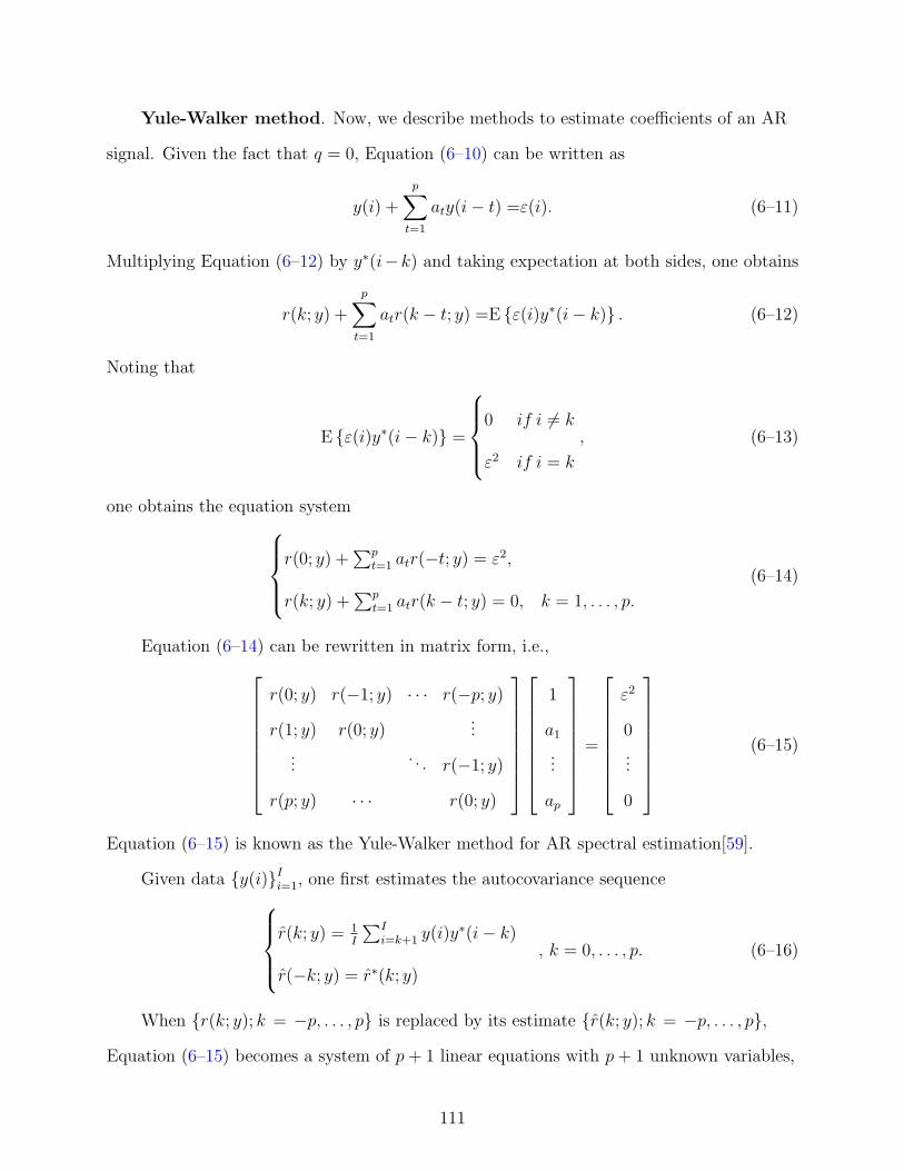
Yule-Walker method. Now, we describe methods to estimate coefficients of an AR

signal. Given the fact that q = 0, Equation (6–10) can be written as

y(i) +

p∑t=1

aty(i− t) =ε(i). (6–11)

Multiplying Equation (6–12) by y∗(i−k) and taking expectation at both sides, one obtains

r(k; y) +

p∑t=1

atr(k − t; y) =E ε(i)y∗(i− k) . (6–12)

Noting that

E ε(i)y∗(i− k) =

0 if i 6= k

ε2 if i = k

, (6–13)

one obtains the equation system

r(0; y) +∑p

t=1 atr(−t; y) = ε2,

r(k; y) +∑p

t=1 atr(k − t; y) = 0, k = 1, . . . , p.

(6–14)

Equation (6–14) can be rewritten in matrix form, i.e.,

r(0; y) r(−1; y) · · · r(−p; y)

r(1; y) r(0; y)...

.... . . r(−1; y)

r(p; y) · · · r(0; y)

1

a1

...

ap

=

ε2

0

...

0

(6–15)

Equation (6–15) is known as the Yule-Walker method for AR spectral estimation[59].

Given data y(i)Ii=1, one first estimates the autocovariance sequence

r(k; y) = 1I

∑Ii=k+1 y(i)y∗(i− k)

r(−k; y) = r∗(k; y)

, k = 0, . . . , p. (6–16)

When r(k; y); k = −p, . . . , p is replaced by its estimate r(k; y); k = −p, . . . , p,Equation (6–15) becomes a system of p + 1 linear equations with p + 1 unknown variables,

111

i.e., ε2, a1, . . ., ap. Its solution is

a1

...

ap

=−

r(0; y) · · · r(−p + 1; y)

.... . .

...

r(p− 1; y) · · · r(0; y)

−1

r(1)

...

r(p)

, (6–17)

ε2 =r(0; y) +

p∑t=1

r(−t; y)at. (6–18)

Levinson-Durbin algorithm (LDA). The direct solution of Yule-Walker method,

i.e., Equations (6–17) and (6–18), is not good enough in terms of time complexity.

Equation (6–17) computes the inversion of covariance matrix, whose time complexity is

O (p3)[60, page 755]. In addition, in most applications, there is no a priori information

about the true order p. To cope with that, the Yule-Walker system of equations,

Equation (6–15), has to be solved for p = 1 up to p = pmax, where pmax is some

prespecified maximum order. The time complexity is O (p4max).

In this paper, we use the Levinson-Durbin Algorithm (LDA)[59]to reduce time

complexity. It estimates AR signal coefficients recursively in the order p. To facilitate

further discussion and to emphasize the order p, we denote

Rp+14=

r(0; y) r(−1; y) · · · r(−p; y)

r(1; y) r(0; y) · · · r(−p + 1; y)

.... . .

...

r(p; y) · · · r(1; y) r(0; y)

, (6–19)

ap4=

a1

...

ap

, (6–20)

112

and ε2p the power of noise of the AR(p) signal. Thus, one can rewrite Equation (6–15) as

Rp+1

1

ap

=

ε2p

0

(6–21)

1. function LDA(. . .)2. Argument 1: data, y(i)I

i=1.3. Argument 2: order, p.4. Return: parameters of AR(p) model, ap and ε2

p.5.

r(k; y) =1

I

I∑

i=k+1

y(i)y∗(i− k), for ∀ k = 0, 1, . . . , p (6–22)

6.

r′1 = a1 = −r(1; y)

r(0; y)(6–23)

7.

ε21 = r(0; y)− |r(1; y)|2

r(0; y)(6–24)

8. for t ← 1, . . . , p9.

rt4= [r∗(t; y), r∗(t− 1; y), · · · , r∗(1; y)]T (6–25)

at4= [at, at−1, · · · , a1]

T (6–26)

r′t+1 =− r(t + 1; y) + rtat

ε2t

(6–27)

ε2t+1 =ε2

t

(1−

∣∣r′t+1

∣∣2)

(6–28)

at+1 =

[at

0

]+ r′t+1

[at

1

](6–29)

10. end for

Figure 6-3. Levinson-Durbin Algorithm.

Figure 6-3 gives the LDA algorithm to estimate coefficients of AR(p) model given

data y(i)Ii=1.

113

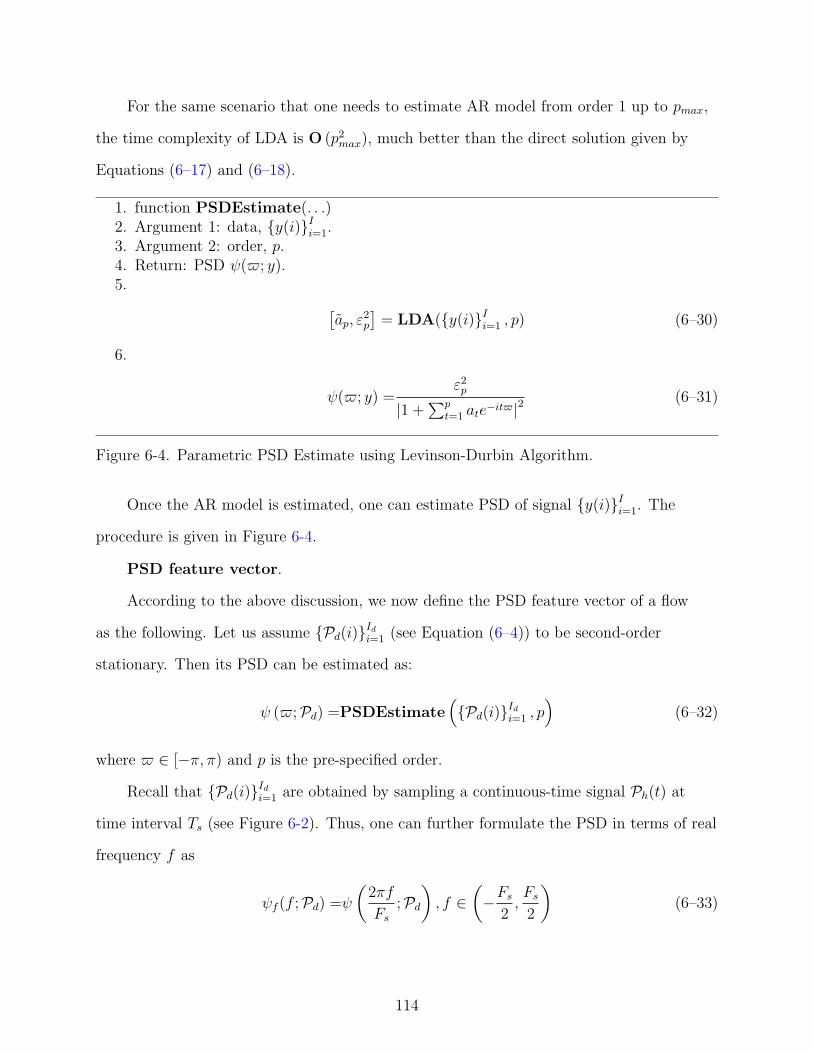
For the same scenario that one needs to estimate AR model from order 1 up to pmax,

the time complexity of LDA is O (p2max), much better than the direct solution given by

Equations (6–17) and (6–18).

1. function PSDEstimate(. . .)2. Argument 1: data, y(i)I

i=1.3. Argument 2: order, p.4. Return: PSD ψ($; y).5.

[ap, ε

2p

]= LDA(y(i)I

i=1 , p) (6–30)

6.

ψ($; y) =ε2

p

|1 +∑p

t=1 ate−it$|2 (6–31)

Figure 6-4. Parametric PSD Estimate using Levinson-Durbin Algorithm.

Once the AR model is estimated, one can estimate PSD of signal y(i)Ii=1. The

procedure is given in Figure 6-4.

PSD feature vector.

According to the above discussion, we now define the PSD feature vector of a flow

as the following. Let us assume Pd(i)Id

i=1 (see Equation (6–4)) to be second-order

stationary. Then its PSD can be estimated as:

ψ ($;Pd) =PSDEstimate(Pd(i)Id

i=1 , p)

(6–32)

where $ ∈ [−π, π) and p is the pre-specified order.

Recall that Pd(i)Id

i=1 are obtained by sampling a continuous-time signal Ph(t) at

time interval Ts (see Figure 6-2). Thus, one can further formulate the PSD in terms of real

frequency f as

ψf (f ;Pd) =ψ

(2πf

Fs

;Pd

), f ∈

(−Fs

2,Fs

2

)(6–33)

114

where Fs = 1Ts

. Equation (6–33) shows the relationship between the periodic components

of a stochastic process in the continuous-time domain and the shape of its PSD in the

frequency domain.

ψf (f ;Pd) is a continuous function in frequency domain. To handle it in a computer,

we need to do sampling in frequency domain. In other words, we select a series of

frequencies,

0 ≤ f1 < f2 < · · · < fM ≤ Fs

2, (6–34)

and define the PSD feature vector as

~ψ =

[ψf (f1;Pd) , ψf (f2;Pd) , ψf (fM ;Pd)

]T

. (6–35)

~ψ ∈ RM is the feature vector we use to perform classification.

In the next Section, we introduce a new technique that we use to translate the

characteristic of these high-dimensional feature vectors into a more tractable low

dimensional space.

6.3 Subspace Decomposition and Bases Identification on PSD Features

In many scientific and engineering problems, the data of interest can be viewed

as drawn from a mixture of geometric or statistical models instead of a single one.

Such data are often referred to in different contexts as “mixed,” or “multi-modal,” or

“multi-model,” or “heterogeneous,” or “hybrid.” Subspace decomposition is a general

method for modeling and segmenting such mixed data using a collection of subspaces,

also known in mathematics as a subspace arrangement. By introducing certain new

algebraic models and techniques into data clustering, traditionally a statistical problem,

the subspace decomposition methodology offers a new spectrum of algorithms for data

modeling and clustering that are in many aspects more efficient and effective than (or

complementary to) traditional methods, e.g., principle component analysis (PCA),

Expectation Maximization (EM), and K-Means clustering.

115

As illustrated in Figure 6-1, we collect voice and video training flows during the

training phase. After processing the raw packet data through the feature extraction

module via PSD, one obtains two sets of feature vectors,

Ψ(1) 4=

~ψ1(1), ~ψ1(2), . . . , ~ψ1 (N1)

, (6–36)

which is obtained through voice training data, where N1 is the number of voice flows; and

Ψ(2) 4=

~ψ2(1), ~ψ2(2), . . . , ~ψ2 (N2)

, (6–37)

which is obtained through video training data, where N2 is the number of video flows.

To facilitate further discussion, let us also regard Ψ(i) as a M ×Ni matrix, for i = 1, 2,

where each column is a feature vector. In other words, Ψ(i) ∈ RM×Ni .

In this section, we present techniques to identify the low dimensional subspaces

embedded in RM , for both Ψ1 and Ψ2.

There are a lot of low dimensional subspace identification schemes, such as Principal

Components Analysis (PCA) [61] and Metric Multidimensional Scaling (MDS) [62], which

identify linear structure, and ISOMAP [63] and Locally Linear Embedding (LLE)[64],

which identify non-linear structure.

Unfortunately, all these methods assume that data are embedded in one single

low-dimensional subspace. This assumption is not always true. For example, as different

software uses different voice coding, it is more reasonable to assume that the PSD feature

vector of voice traffic is a random vector generated from a mixture model than a single

model. In such case, it is more likely that there are several subspaces in which the feature

vectors are embedded. The same holds for video feature vectors.

As a result, a better scheme is to first, cluster the trained feature vectors into several

groups, known as subspace decomposition; and second, to identify the subspace structure

of each group, known as subspace bases identification. We describe the two steps in the

following sections.

116

6.3.1 Subspace Decomposition Based on Minimum Coding Length

The purpose of subspace decomposition is to partition the data set

Ψ =

~ψ(1), ~ψ(2), . . . , ~ψ (N)

(6–38)

into non-overlapping K subsets such that

Ψ =Ψ1 ∪Ψ2 ∪ · · · ∪ΨK . (6–39)

Hong[65] proposed a method to decompose subspaces according to the minimum coding

length criteria. The idea is to view the data segmentation problem from the perspective of

data coding/compression.

Suppose one wants to find a coding scheme, C, which maps data in Ψ ∈ RM×N to

bit sequence. As all elements are real numbers, infinite long bit sequence is needed to

decode without error. Hence, one has to specify the tolerable decoding error, ε, to obtain a

mapping with finite coding length, i.e.,

∥∥∥~ψn − C−1(C

(~ψn

))∥∥∥2

≤ ε2, for ∀n = 1, . . . , N. (6–40)

Then the coding length of the coding scheme C is a function

LC : RM×N → Z+. (6–41)

It is proven [65] that the coding length is up bounded by

LC (Ψ) ≤L (Ψ) =N + K

2log2 det

(I +

K

Nε2ΨΨT

)+

K

2log2

(1 +

µTΨµΨ

ε2

), (6–42)

where

µΨ =1

N

N∑i=1

~ψ(i), (6–43)

Ψ =[~ψ(1)− µΨ, . . . , ~ψ(N)− µΨ

]. (6–44)

117

The optimal partition (see Equation (6–39)), in terms of minimum coding length

criteria, should minimize coding length of the segmented data, i.e.,

minΠLC (Ψ; Π) = min

Π

K∑

k=1

LC (Ψk) +K∑

k=1

|Ψk|[− log2

(Ψk

K

)], (6–45)

where Π denotes the partition scheme. The first term in Equation (6–45) is the summation

of coding length of each group, and the second one is the number of bits needed to

encoding membership of each item of Ψ in the K groups.

The optimal partition is achieved in the following way. Let the segmentation scheme

be represented by the membership matrix,

Πk4= diag ([π1k, π2k, . . . , πNk]) ∈ RN×N , (6–46)

where πnk denotes the probability that vector ~ψ(n) belongs to subset k, such that

K∑

k=1

πnk = 1, for ∀n = 1, . . . , N (6–47)

and diag(·) denotes converting a vector to a diagonal matrix.

Hong[65, page 34] proved that the coding length is bounded as follows.

LC (Ψ; Π)

≤K∑

k=1

[tr (Πk) + K

2log2 det

(I +

K

tr (Πk) ε2ΨΠkΨ

T

)]

+K∑

k=1

[tr (Πk)

(− log2

tr (Πk)

N

)]

4=L(Ψ; Π), (6–48)

where tr (·) denotes the trace of a matrix, and det (·) denotes matrix determinant.

Combining Equations (6–45) and (6–48), one achieves a minimax criterion

Π = arg minΠ

[maxCLC (Ψ; Π)

]= arg min

ΠL(Ψ; Π). (6–49)

118

Then for ∀ψn ∈ Ψ, ψn ∈ Ψk after segmentation if and only if

k = arg maxk

πnk. (6–50)

1. function MCLPartition(. . .)

2. Argument 1: set of feature vectors, Ψ =

~ψ(1), . . . , ~ψ (N)

3. Return: partition of Ψ,

Π = Ψ1, . . . , ΨK ; Ψ1 ∪ . . . ∪ΨK = Ψ, Ψi ∩Ψj = ∅ for ∀i 6= j,

.4. Initialization:

Π =

~ψ(1)

,

~ψ(2)

, . . . ,

~ψ(N)

,

5. while true do6.

〈π1, π2〉 = arg minπ∗1∈Π,π∗2∈Π

L (π∗1 ∪ π∗2)− L (π∗1, π∗2) (6–51)

7. if L (π∗1 ∪ π∗2)− L (π∗1, π∗2) ≥ 0 then

8. break9. else

10. Π = (Π \ π1, π2) ∪ π1 ∪ π211. end if12. end while13. return Π

Figure 6-5. Pairwise steepest descent method to achieve minimal coding length.

There is no closed form solution for Equation (6–49). Hong[65, page41] proposed a

pairwise steepest descent method to solve it (Figure 6-5). It works in a bottom-up way.

It starts with a partition scheme that assigns each element of Ψ to a partition. Then, at

each iteration, the algorithm finds two subsets of feature vectors such that by merging

these two subsets, one can decrease the coding length the most (Equation (6–51)). This

procedure stops when no further decrease of coding length can be achieved by merging any

two subsets.

Using the above method, we obtain a partition of voice feature vector set Ψ(1),

119

Ψ(1) = Ψ(1)1 ∪ · · · ∪Ψ

(1)K1

, (6–52)

and a partition of video feature vector set Ψ(2),

Ψ(2) = Ψ(2)1 ∪ · · · ∪Ψ

(2)K2

. (6–53)

Next, we describe the method to identify subspace bases in each of the segmentations.

6.3.2 Subspace Bases Identification

In this section, we use PCA[61] algorithm to identify subspace bases for each

segmentation,

Ψ

(i)k ; k = 1, . . . , Ki, i = 1, 2

, (6–54)

obtained in the previous section. The basic idea is to identify uncorrelated bases and

choose those bases with dominant energy. Figure 6-6 shows the algorithm.

1. function[~µ, U , Σ, U , Σ

]= IdentifyBases

(Ψ ∈ RM×N , δ

)

2. ~µ = 1|Ψ|

∑~ψ∈Ψ

~ψ

3. Ψ =[~ψ1 − ~µ, ~ψ2 − ~µ, . . . , ~ψ|Ψ| − ~µ

]

4. Do eigenvalue decomposition on ΨΨT such that

ΨΨT =UΣUT , (6–55)

where U 4= [~u1, · · · , ~uM ], Σ

4= diag ([σ2

1, . . . , σ2M ]), and σ2

1 ≥ σ22 ≥ · · · ≥ σ2

M .

5. J = arg minJ∑J

m=1 σ2(m) ≥ δ∑M

m=1 σ2(m)

6. U = [~u1, ~u2, . . . , ~uJ−1]7. U = [~uJ , ~uJ+1, . . . , ~uM ]8. Σ = diag

([σ2

1, . . . , σ2J−1

])9. Σ = diag

([σ2J , . . . , σ2

M

])10. end function

Figure 6-6. Function IdentifyBases identifies bases of subspace.

In Figure 6-6, argument Ψ represents the feature vector set of one segmentation and

δ is a user defined parameter which specifies the percentage of energy retained, e.g., 90%

120

or 95%. The algorithm returns 5 variables. ~µ represents the sampled mean of all feature

vectors. It is the origin of the identified subspace. The columns of U are the bases with

dominant energy (i.e.,variance), whose corresponding variances are denoted by Σ. These

bases determine the identified low dimensional subspace spanned by Ψ. The columns of

U compose the null space of the previous subspace, whose corresponding variances are Σ.

The last two outputs are required to calculate the distance of an ongoing feature vector to

the subspace, which will be described in Section 6.4.

Applying the function IdentifyBases on all segmentations, we obtain

[~µ

(i)k , U (i)

k , Σ(i)k , U (i)

k , Σ(i)k

]=IdentifyBases(Ψ

(i)k ) (6–56)

for ∀k = 1, . . . , Ki, ∀i = 1, 2. These are the outputs of subspace identification module, and

hence the results of training phase, in Figure 6-1.

During the classification phase, these outputs are used as system parameters, which

will be presented in the next section.

6.4 Voice/Video Classifier

In Section 6.3, we presented an approach to identify subspaces spanned by PSD

feature vectors of training voice and video flows. Specifically, one obtains the following

parameters:

[~µ

(i)k , U (i)

k , Σ(i)k , U (i)

k , Σ(i)k

](6–57)

for ∀k = 1, . . . , Ki, ∀i = 1, 2. In this section, we use these parameters to do classification.

During the classification phase, for each ongoing flow F , one composes a sub-flow,

FS, by extracting small packets, i.e., packets smaller than θP , and passes it through PSD

feature extraction module to generate PSD feature vector ~ψ. This is the input to the

voice/video classifier.

The voice/video classifier works in the following way. It first calculates the normalized

distances between ~ψ and all subspaces of both categories. Then it chooses minimum

121

distance to each category. The decision is made by comparing the two distance values to

two thresholds, θA and θV respectively for voice and video. Figure 6-7 shows the procedure

of the voice/video classifier.

1. function type = VoiceVideoClassify(

~ψ, θA, θV

)

2. For ∀i = 1, 2, ∀k = 1, . . . , Ki

d(i)k = NormalizedDistance

(~ψ, ~µ

(i)k , U (i)

k , Σ(i)k

)

.3. For ∀i = 1, 2,

di = mink

d(i)k

.4. if d1 < θA and d2 > θV

5. type = VOICE.6. else if d1 > θA and d2 < θV

7. type = VIDEO.8. else9. type = “DON’T KNOW”, i.e., neither voice nor video.

10. end if11. end function

12. function d = NormalizedDistance(

~ψ, ~µ, U , Σ)

13. d =(

~ψ − ~µ)T

UΣ−1UT(

~ψ − ~µ)

14. end function

Figure 6-7. Function VoiceVideoClassify determines whether a flow with PSD featurevector ~ψ is of type voice or video or neither. θ1 are θ2 are two user-specified thresholdarguments. Function voicevideoClassify uses Function NormalizedDistance to calculatenormalized distance between a feature vector and a subspace.

Note that, in Function VoiceVideoClassify, line 7, when we detect flow type to be

video, the flow may also carry voice traffic. The reason is discussed in Section 6.1.3.

From lines 2 and 13 in Figure 6-7, the time complexity of function VoiceVideoClassify

is

O((K1 + K2)M

2). (6–58)

122

6.5 Experiment Results

In this section, we demonstrate the experiment results of applying the system

presented in Figure 6-1 to network traffic classification. Before that, we first describe

experiment settings in Section 6.5.1.

6.5.1 Experiment Settings

We perform four sets of experiments. In Section 6.5.2, two sets of experiments are

conducted on traffic generated by Skype. In Section 6.5.3, other two sets of experiments

are conducted on traffic generated by Skype, MSN, and GTalk.

For each set of the experiments, we use Receiver Operating Characteristics (ROC)

curves[28, page 107] as the performance metric. ROC curve is a curve of detection

probability, PD, vs. false alarm probability, PFA, where,

PD|H4=P (The estimated state of nature is H|The true state of nature is H) , (6–59)

PFA|H4=P (The estimated state of nature is H|The true state of nature is not H) , (6–60)

where H can be voice, video, file+voice, and file+video. By tuning parameters θσ, θA, and

θV ( see Figure 6-7), one is able to generate ROC curve.

During the experiments, we collected network traffic from three applications, i.e.,

Skype, MSN, and GTalk. For each application, traffic was collected in two scenarios. For

the first scenario, two lab computers located in University A and University B respectively

were communicating with each other. There was direct connection between two peers. For

the second one, we used a firewall to block direct connection between the two peers such

that the application was forced to use relay nodes.

To do classification, we chose first 10 seconds of each flow, i.e., Amax ≤ 10 seconds.

We set Ts = 0.5 milliseconds. Hence, Id = 20, 000.

123

6.5.2 Skype Flow Classification

In this section, we conduct experiments on Skype traffic. We first consider the

scenario when each Skype flow carries one type of traffic. In other words, in this set of

experiments, one flow is of type VOICE, VIDEO, or none of the above.

Figure 6-8 shows the ROC curves of classifying voice and video flows.

0 0.2 0.4 0.6 0.8 10.9

0.91

0.92

0.93

0.94

0.95

0.96

0.97

0.98

0.99

1

PFA

PD

(a)

0 0.2 0.4 0.6 0.8 10.9

0.91

0.92

0.93

0.94

0.95

0.96

0.97

0.98

0.99

1

PFA

PD

(b)

Figure 6-8. The ROC curves of single-typed flows generated by Skype, (a) VOICE and (b)VIDEO.

We then conduct experiments on hybrid Skype flows. In other words, each flow

may be of type VOICE, VIDEO, FILE+VOICE, FILE+VIDEO, or none of the above.

Figure 6-9 plots the ROC curves of these five types, respectively.

6.5.3 General Flow Classification

Now, let us do the same experiments on network traffic generated by Skype, MSN,

and GTalk, as these are very common applications at present. In other words, a voice flow

now can be a VoIP flow generated by Skype, MSN, or GTalk. So are video flows. Note

that, GTalk does not support video conference. Similarly, two sets of experiments are

conducted, one on single-typed flows and the other on hybrid flows.

124

0 0.2 0.4 0.6 0.8 10.9

0.91

0.92

0.93

0.94

0.95

0.96

0.97

0.98

0.99

1

PFA

PD

(a)

0 0.2 0.4 0.6 0.8 10.9

0.91

0.92

0.93

0.94

0.95

0.96

0.97

0.98

0.99

1

PFA

PD

(b)

0 0.2 0.4 0.6 0.8 10.5

0.55

0.6

0.65

0.7

0.75

0.8

0.85

0.9

0.95

1

PFA

PD

(c)

0 0.2 0.4 0.6 0.8 10.5

0.55

0.6

0.65

0.7

0.75

0.8

0.85

0.9

0.95

1

PFA

PD

(d)

Figure 6-9. The ROC curves of hybrid flows generated by Skype, (a) VOICE, (b) VIDEO,(c) FILE+VOICE, and (d) FILE+VIDEO.

Similar to Section 6.5.2, we first consider the scenario when each flow carries one type

of traffic. By tuning the thresholds, θσ, θA, and θV , we generate ROC curves of classifying

voice and video flows (Figure 6-10).

We then conduct experiments on hybrid flows. Figure 6-11 shows the ROC curves of

classifying VOICE, VIDEO, FILE+VOICE, and FILE+VIDEO flows.

6.5.4 Discussion

To better understand Figs. 6-8, 6-9, 6-10, and 6-11, we show some typical values of

PD and PFA pairs in Table 6-1. One can see the following phenomena from Table 6-1.

125

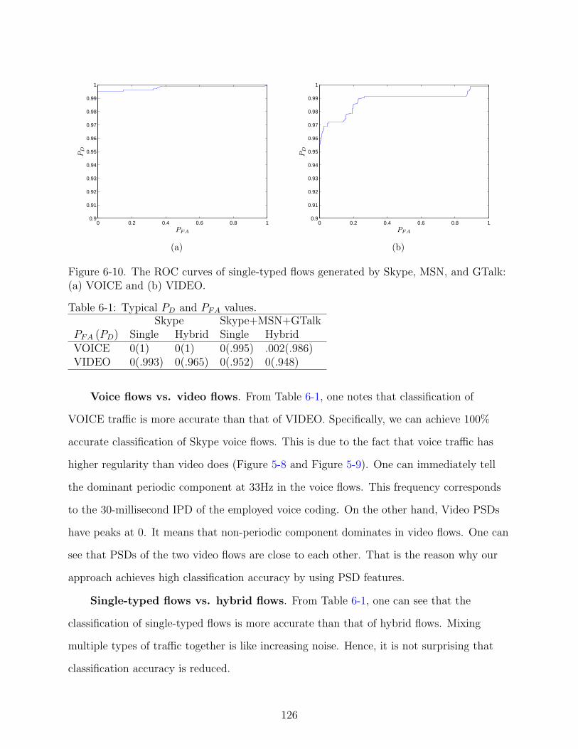
0 0.2 0.4 0.6 0.8 10.9

0.91

0.92

0.93

0.94

0.95

0.96

0.97

0.98

0.99

1

PFA

PD

(a)

0 0.2 0.4 0.6 0.8 10.9

0.91

0.92

0.93

0.94

0.95

0.96

0.97

0.98

0.99

1

PFA

PD

(b)

Figure 6-10. The ROC curves of single-typed flows generated by Skype, MSN, and GTalk:(a) VOICE and (b) VIDEO.

Table 6-1: Typical PD and PFA values.Skype Skype+MSN+GTalk

PFA (PD) Single Hybrid Single HybridVOICE 0(1) 0(1) 0(.995) .002(.986)VIDEO 0(.993) 0(.965) 0(.952) 0(.948)

Voice flows vs. video flows. From Table 6-1, one notes that classification of

VOICE traffic is more accurate than that of VIDEO. Specifically, we can achieve 100%

accurate classification of Skype voice flows. This is due to the fact that voice traffic has

higher regularity than video does (Figure 5-8 and Figure 5-9). One can immediately tell

the dominant periodic component at 33Hz in the voice flows. This frequency corresponds

to the 30-millisecond IPD of the employed voice coding. On the other hand, Video PSDs

have peaks at 0. It means that non-periodic component dominates in video flows. One can

see that PSDs of the two video flows are close to each other. That is the reason why our

approach achieves high classification accuracy by using PSD features.

Single-typed flows vs. hybrid flows. From Table 6-1, one can see that the

classification of single-typed flows is more accurate than that of hybrid flows. Mixing

multiple types of traffic together is like increasing noise. Hence, it is not surprising that

classification accuracy is reduced.

126

0 0.2 0.4 0.6 0.8 10.5

0.55

0.6

0.65

0.7

0.75

0.8

0.85

0.9

0.95

1

PFA

PD

(a)

0 0.2 0.4 0.6 0.8 10.5

0.55

0.6

0.65

0.7

0.75

0.8

0.85

0.9

0.95

1

PFA

PD

(b)

0 0.2 0.4 0.6 0.8 10

0.1

0.2

0.3

0.4

0.5

0.6

0.7

0.8

0.9

1

PFA

PD

(c)

0 0.2 0.4 0.6 0.8 10

0.1

0.2

0.3

0.4

0.5

0.6

0.7

0.8

0.9

1

PFA

PD

(d)

Figure 6-11. The ROC curves of hybrid flows generated by Skype, MSN, and GTalk: (a)VOICE, (b) VIDEO, (c) FILE+VOICE, and (d) FILE+VIDEO.

One application vs. multiple applications. One further notes that classification

of Skype flows is more accurate than that of flows generated from general applications, i.e.,

Skype, MSN, and GTalk.

Empirically, we found that Skype flows are similar to GTalk flows, but quite different

from MSN. For example, both Skype and GTalk voice flows have about 33-millisecond

inter-arrival time, whereas MSN voice flow has approximately 25-millisecond inter-arrival

time.

127

When these flows are mixed together, classification accuracy is reduced. But the

accuracy reduction is acceptable. Specifically, for hybrid voice traffic at PFA ≈ 0, PD is

reduced from 1 to 0.986; for hybrid video traffic, it is from 0.965 to 0.948.

This shows that our approach is robust. The robustness results from the fact that the

subspace identification module, as presented in Section 6.3, decomposes multiple subspaces

in the original high-dimensional feature space. As a result, PSD feature vectors of Skype

and GTalk are likely to be within different subspaces than those of MSN. Therefore, we

can still classify traffic accurately.

6.6 Summary

In this chapter, we describe the VOVClassifier system to do network classification.

VOVClassifier is composed of four components, feature summary generator, feature

extractor, subspace generator, and voice/video classifier. The novelty of VOVClassifier is

• modeling a network flow by a stochastic process;

• estimating PSD feature vector to extract the regularities residing in voice and videotraffic;

• decomposing subspaces of training feature vectors followed by bases identification;

• using minimum distance to subspace as the similarity metric to perform classification.

Experiment results demonstrate the effectiveness and robustness of our approach.

Specifically, we show that classification of voice traffic is more accurate than that of video

traffic; classification of single-typed flows is more accurate than that of hybrid flows;

and classification of pure Skype flows is more accurate than that of flows generated from

multiple applications (e.g., Skype, MSN, and GTalk).

128

CHAPTER 7CONCLUSION AND FUTURE WORK

7.1 Summary of Network Centric Anomaly Detection

In the first part of our study, we presented our achievement on network centric

anomaly detection. We first proposed a novel edge-router based framework to robustly

and efficiently detect network anomalies in the first place they happen. The key idea is

to exploit spatial and temporal correlation of abnormal traffic. The motivation of our

framework design is to use both spacial and temporal correlation among edge routers. The

framework consists of three types of components (i.e., traffic monitors, local analyzers,

and a global analyzer). Traffic monitors summarize traffic information on each single link

between edge router and user subnet. Local analyzers collect information on edge routers,

which is provided by traffic monitors, and reports to the global analyzer. The global

analyzer has a global view of the whole autonomous system and makes final decision. The

advantages of our framework design are the following.

1. It is deployed on edge routers instead of systems of end users, such that it can detectnetwork anomalies in the first place they enter an AS.

2. It has no burden on core routers;

3. It is flexible in that detection of network anomalies can be made both locally andglobally;

4. It is capable of detecting low volume network anomalies accurately by exploitingspatial correlations among edge routers.

We then presented feature extraction for network anomaly detection. Based on

the framework, we designed the hierarchical feature extraction architecture. Different

components extract different features. For example, traffic monitors can extract features

such as packet rate, data rate, and SYN/FIN ratio. Local analyzers are able to extract

features such as SYN/SYN-ACK ratio, round-trip time, and two-way matching features

on one edge router. The global analyzer can extract two-way matching features from

the whole autonomous system. Specifically, we focus on the novel type of features,

129

the two-way matching features, proposed by us. This type of features uses both the

temporal and spacial information carried in network traffic. It is a very effective indicator

of network anomaly associated with spoofed source IP address. We designed a novel

data structure, referred to as Bloom filter array, to efficiently extract two-way matching

features. Different from the existing works, our data structure has the following properties:

1) dynamic Bloom filter, 2) combination of a sliding window with the Bloom filter, and

3) using insertion-removal pairs to enhance the Bloom filter with a removal operation.

Our analysis and simulation demonstrate that the proposed data structure has a better

space/time trade-off than conventional algorithms.

In the end, we applied the machine learning technology to network anomaly detection.

Specifically, we used Bayesian model to determine the state of each edge router, normal

or abnormal. Traditionally, edge routers are regarded as independent. It is incapable to

detect low-traffic network anomaly. Straightforward improvement over this independent

model is to regard edge routers to be dependent on each other. However, this method has

an exponential time complexity to determine the edge router states, i.e., O (2κ), where

κ is the number of edge routers. We proposed the hidden Markov tree (HMT) to model

the correlations among edge routers. It takes advantages of employing dependence among

edge routers while has almost linear time complexity, i.e., O (Bκ), where B is the number

of child nodes of each non-leaf node in the HMT. Our machine learning scheme has the

following nice properties:

• In addition to detecting network anomalies having high-data-rate on a link, ourscheme is also capable of accurately detecting attacks having low-data-rate onmultiple links. This is due to exploitation of spatial correlation of network anomalies.

• Our scheme is robust against time-varying traffic patterns, owing to powerful machinelearning techniques.

• Our scheme can be deployed in large-scale high-speed networks, thanks to use ofBloom filter array to efficiently extract features.

130

Our simulation results show that the proposed framework can detect DDoS attacks

even if the volume of attack traffic on each link is extremely small (i.e., 1%). Especially,

for the same false alarm probability, our scheme has a detection probability of 0.97,

whereas the existing scheme has a detection probability of 0.17, which demonstrates the

superior performance of our scheme.

7.2 Summary of Network Centric Traffic Classification

We then presented our research on network centric traffic classification, specifically, to

detect and classify voice and video data streams.

We first motivated the significance and points out the challenges of this issue, and

shows weakness of existing solutions. With the emergence of software using user specified

ports or dynamic ports, traffic classification based on TCP and UDP port numbers is

no longer valid. Other methods based on reconstructions of session and application

information from packet contents impose significant complexity and processing load on

the classification device. In addition, they are incapable to classify encrypted traffic. A

new emerging tendency in the research community to approach this problem is to rely

on pattern classification techniques. However, existing machine learning technologies are

not able to distinguish between voice and video traffic. In the research, we also proposed

a novel problem that one network flow may carry multiple types of sessions, such as

Skype uses one connection to carry voice, video, chat, and file transfer at the same time.

This increases the difficulties of traffic classification. To our best knowledge, no existing

literature has ever considered this problem. Our intuition to approach this problem is to

employ regularities residing in multimedia traffic. We also illustrates four types of metrics

to measure the regularities, i.e.,

1. packet inter-arrival time and packet size in time domain;

2. packet inter-arrival time in frequency domain;

3. packet size in frequency domain;

131

4. combining packet inter-arrival time and packet size in frequency domain.

It turns out that the last one is the most distinctive feature for classifying voice and

video traffic.

We then presented the VOVClassifier system to classify voice and video traffic.

VOVClassifier is composed of four major modules that operate in cascade, flow summary

generator, feature extractor, voice / video subspace generator, and voice / video classifier.

The novelty of VOVClassifier is that

• we combine packet inter-arrival times and packet sizes of a network flow and model itby a stochastic process;

• we estimate PSD feature vector to extract regularities residing in voice and videotraffic;

• we use minimum coding length to decompose subspaces from the training featurevectors and principal component analysis to identify bases of each subspace;

• we use minimum distance to subspaces as the similarity metric to perform classification.

The experiment results demonstrate the effectiveness and robustness of our approach.

132

APPENDIX APROOFS

A.1 Equation (4–31)

Proof:

∑

u′∈0,1P

(Ωi = u|Ωρ(i) = u′

)Υρ(i)(u

′)p(φρ(i)|uρ(i) = u′)

=∑

u′∈0,1P

(Ωi = u|Ωρ(i) = u′

)p(Ωρ(i) = u′, ~φT\ρ(i)

)p(φρ(i)|Ωρ(i) = u′)

=∑

u′∈0,1p(Ωi = u, Ωρ(i) = u′, ~φT\i

)

=p(Ωi = u, ~φT\i)

=Υi(u). (A–1)

A.2 Equation (4–32)

Proof:

p(φi|Ωi = u)∏

j∈ν(i)

∑

u′∈0,1P (Ωj = u′|Ωi = u) υj(u

′)

=p(φi|Ωi = u)∏

j∈ν(i)

∑

u′∈0,1P (Ωj = u′|Ωi = u) p(~φTj

|Ωj = u′)

=p(φi|Ωi = u)∏

j∈ν(i)

p(~φTj|Ωi = u)

=p(~φTi|Ωi = u) = υi(u) (A–2)

133

A.3 Equation (4–33)

Proof:

Υi(u)υi(u)∑u′ Υi(u′)υi(u′)

=p(Ωi = u, ~φT\i

)p(~φT\i

|Ωi = u)

∑u′ p

(Ωi = u′, ~φT\i

)p(~φT\i

|Ωi = u)

=p(Ωi = u, ~φ

)

∑u′ p

(Ωi = u′, ~φ

)

=p(Ωi = u, ~φ

)

p(~φ)

=P (Ωρ(i) = u|~φ) (A–3)

A.4 Equation (4–34)

Proof:

υi(u)υρ(i)(u′)P

(Ωi = u|Ωρ(i) = u′

)Υρ(i)(u

′)

[∑

u′′ Υi(u′′)υi(u′′)][∑

u′′ P(Ωi = u′′|Ωρ(i) = u′

)υi(u′′)

]

=p(~φTi|Ωi = u

)p(~φTρ(i)

|Ωρ(i) = u′)

P(Ωi = u|Ωρ(i) = u′

)p(Ωρ(i) = u′, ~φT\ρ(i)

)[∑

u′′ p(Ωi = u′′, ~φT\i

)p(~φTi|Ωi = u′′

)] [∑u′′ P

(Ωi = u′′|Ωρ(i) = u′

)p(~φTi|Ωi = u′′

)]

=p(Ωi = u, ~φTi

|Ωρ(i) = u′)

p(Ωρ(i) = u′, ~φT\ρ(i)

)p(~φTρ(i)

|Ωρ(i) = u′)

[∑u′′ p

(Ωi = u′′, ~φ

)] [∑u′′ p

(Ωi = u′′, ~φTi

|Ωρ(i) = u′)]

=p(Ωi = u, Ωρ(i) = u′, ~φTi∪T\ρ(i)

)p(~φTρ(i)

|Ωρ(i) = u′)

p(~φ)

p(~φTi|Ωρ(i) = u′

)

=p(Ωi = u, Ωρ(i) = u′, ~φTi∪T\ρ(i)

)p(~φρ(i)|~φTi

, Ωρ(i) = u′)

p(~φ)

=p(Ωi = u, Ωρ(i) = u′, ~φ

)

p(~φ)

=P (Ωi = u, Ωρ(i) = u′|~φ) (A–4)

134

REFERENCES

[1] P. Mockapetris, “Domain names - concepts and facilities,” RFC 1034.

[2] P. Mockapetris, “Domain names - implementation and specification,” RFC 1035.

[3] “Video on demand,” Wikipedia. [Online]. Available: http://en.wikipedia.org/wiki/Video on demand

[4] D. Wu, Y. T. Hou, W. Zhu, Y.-Q. Zhang, and J. M. Peha, “Streaming video overthe internet: Approaches and directions,” IEEE Trans. Circuits Syst. Video Technol.,vol. 11, pp. 282–300, Mar. 2001.

[5] K. Nichols, S. Blake, F. Baker, and D. Black, “Definition of the differentiated servicesfield (ds field) in the ipv4 and ipv6 headers,” RFC 2474.

[6] S. Blake, D. Black, M. Carlson, E. Davies, Z. Wang, and W. Weiss, “An architecturefor differentiated services,” RFC 2475.

[7] P. Almquist, “Type of service in the internet protocol suite,” RFC 1349.

[8] S. S. Kim, A. L. N. Reddy, and M. Vannucci, “Detecting traffic anomalies usingdiscrete wavelet transform,” in Proceedings of International Conference on InformationNetworking (ICOIN), vol. III, Busan, Korea, Feb. 2004, pp. 1375–1384.

[9] C.-M. Cheng, H. T. Kung, and K.-S. Tan, “Use of spectral analysis in defense againstdos attacks,” in Proceedings of IEEE Globecom 2002, vol. 3, Taipei, Taiwan, Nov.2002, pp. 2143–2148.

[10] A. Hussain, J. Heidemann, and C. Papadopoulos, “A framework for classifying denialof service attacks,” in Proceedings of ACM SIGCOMM, Karlsruhe, Germany, Aug.2003.

[11] H. Wang, D. Zhang, and K. G. Shin, “Detecting SYN flooding attacks,” in Proc. IEEEINFOCOM’02, New York City, NY, June 2002, pp. 1530–1539.

[12] T. Peng, C. Leckie, and K. Ramamohanarao, “Detecting distributed denial of serviceattacks using source IP address monitoring,” Department of Computer Science andSoftware Engineering, The University of Melbourne, Tech. Rep., 2002. [Online].Available: http://www.cs.mu.oz.au/∼tpeng

[13] R. B. Blazek, H. Kim, B. Rozovskii, and A. Tartakovsky, “A novel approach todetection of “denial-of-service” attacks via adaptive sequential and batch-sequentialchange-point detection methods,” in Proc. IEEE Workshop on Information Assuranceand Security, West Point, NY, June 2001, pp. 220–226.

[14] S. Mukkamala and A. H. Sung, “Detecting denial of service attacks using supportvector machines,” in Proceedings of IEEE International Conference on Fuzzy Systems,May 2003.

135

136

[15] S. Savage, D. Wetherall, A. Karlin, and T. Anderson, “Practical network support forip traceback,” in Proc. of ACM SIGCOMM’2000, Aug. 2000.

[16] A. Lakhina, M. Crovella, and C. Diot, “Characterization of network-wide anomaliesin traffic flows,” in Proc. ACM SIGCOMM Conference on Internet Measurement ’04,Oct. 2004.

[17] H. Wang, D. Zhang, and K. G. Shin, “Change-point monitoring for the detectionof dos attacks,” IEEE Transactions on Dependable and Secure Computing, no. 4, pp.193–208, Oct. 2004.

[18] J. Mirkovic and P. Reiher, “A taxonomy of ddos attacks and ddos defense mechanisms,”in Proc. ACM SIGCOMM Computer Communications Review ’04, vol. 34, Apr. 2004,pp. 39–53.

[19] J. B. Postel and J. Reynolds, “File transfer protocol,” RFC 959, Oct. 1985. [Online].Available: http://www.faqs.org/rfcs/rfc959.html

[20] K. Lu, J. Fan, J. Greco, D. Wu, S. Todorovic, and A. Nucci, “A novel anti-ddos systemfor large-scale internet,” in ACM SIGCOMM 2005, Philadelphia, PA, Aug. 2005.

[21] B. H. Bloom, “Space/time trade-offs in hash coding with allowable errors,” Commun.ACM, vol. 13, no. 7, pp. 422–426, July 1970.

[22] L. Fan, P. Cao, J. Almeida, and A. Z. Broder, “Summary cache: A scalable wide-areaweb cache sharing protocol.” IEEE/ACM Trans. Netw., vol. 8, no. 3, June 2000.

[23] F. Chang, W. chang Feng, and K. Li, “Approximate caches for packet classification,”in IEEE INFOCOM 2004, vol. 4, Mar. 2004, pp. 2196–2207.

[24] R. Rivest, “The md5 message-digest algorithm,” RFC 1321, Apr. 1992. [Online].Available: http://www.faqs.org/rfcs/rfc1321.html

[25] MD5 CRYPTO CORE FAMILY, HDL Design House, 2002. [Online]. Available:http://www.hdl-dh.com/pdf/hcr 7910.pdf

[26] D. A. Patterson and J. L. Hennessy, Computer Organization and Design: TheHardware/Software Interface. San Francisco, CA: Morgan Kaufmann, 1998, ch. 5,6.

[27] “Auckland-IV trace data,” 2001. [Online]. Available: http://wand.cs.waikato.ac.nz/wand/wits/auck/4/

[28] L. L. Scharf, Statistical signal processing: detection, estimation, and time seriesanalysis. Addison Wesley, 1991.

[29] R. O. Duda, P. E. Hart, and D. G. Stork, Pattern Classification, 2nd ed.Wiley-Interscience, Oct. 2000.

[30] G. Casella and R. L. Berger, Statistical Inference, 2nd ed. Duxbury Press, June 2001.

137

[31] B. J. Frey, Graphical Models for Machine Learning and Digital Communication.Cambridge, MA: MIT Press, 1998.

[32] M. C. Nechyba, “Maximum-likelihood estimation for mixture models:the em algorithm,,” 2003, course note. [Online]. Available: http://mil.ufl.edu/∼nechyba/ eel6825.f2003/course materials/t4.em theory/em notes.pdf

[33] Y. Weiss, “Correctness of local probability propagation in graphical models withloops,” Neural Computation, vol. 12, pp. 1–4, 2000.

[34] J. S. Yedidia, W. T. Freeman, and Y. Weiss, “Generalized belief propagation,”Advances in Neural Information Processing Systems, vol. 13, pp. 689–695, Dec. 2000.

[35] J. Pearl, Probabilistic Reasoning in Intelligent Systems: Networks of PlausibleInference. Morgan Kaufmann, Sept. 1988.

[36] S. M. Aji and R. J. McEliece, “The generalized distributive law,” IEEE Trans. Inform.Theory, vol. 46, pp. 325–343, Mar. 2000.

[37] T. Richardson, “The geometry of turbo-decoding dynamics,” IEEE Trans. Inform.Theory, vol. 46, pp. 9–23, Jan. 2000.

[38] R. J. McEliece, D. J. C. McKay, and J. F. Cheng, “Turbo decoding as an instanceof pearls belief propagation algorithm,” IEEE J. Select. Areas Commun., vol. 16, pp.140–52, Feb. 1998.

[39] F. Kschischang and B. Frey, “Iterative decoding of compound codes by probabilitypropagation in graphical models,” IEEE J. Select. Areas Commun., vol. 16, pp.219–230, Feb. 1998.

[40] A. J. Viterbi, “Error bounds for convolutional codes and an asymptotically optimumdecoding algorithm,” IEEE Trans. Inform. Theory, vol. 13, pp. 260–269, Apr. 1967.

[41] J. G. DAVID FORNEY, “The viterbi algorithm,” in Proceedings of the IEEE, vol. 61,Mar. 1973, pp. 268–278.

[42] L. R. RABINER, “A tutorial on hidden markov models and selected applications inspeech recognition,” in Proceedings of the IEEE, vol. 77, Feb. 1989, pp. 257–286.

[43] D. Moore, K. Keys, R. Koga, E. Lagache, and k claffy, “The CoralReef software suiteas a tool for system and network administrators,” in Usenix LISA. (2001), Dec. 2001.[Online]. Available: citeseer.ist.psu.edu/moore01coralreef.html

[44] C. Logg, “Characterization of the traffic between slac and the internet,” July2003. [Online]. Available: http://www.slac.stanford.edu/comp/net/slac-netflow/html/SLAC-netflow.html

[45] I. A. N. Authority, “Port numbers,” Aug. 2006. [Online]. Available:http://www.iana.org/assignments/port-numbers

138

[46] T. Karagiannis, A. Broido, N. Brownlee, kc claffy, and M. Faloutsos, “Is p2p dying orjust hiding?” in IEEE Globecom 2004, 2004.

[47] S. Sen, O. Spatscheck, and D. Wang, “Accurate, scalable in nettwork identification ofp2p traffic using application signatures,” in WWW, 2004.

[48] K. Wang, G. Cretu, and S. J. Stolfo, “Anomalous payload-based network intrusiondetection,” in 7th International Symposium on Recent Advanced in IntrusionDetection, Sept. 2004, pp. 201–222.

[49] M. Roughan, S. Sen, O. Spatscheck, and N. Duffield, “Class-of-service mapping for qos:A statistical signature-based approach to ip traffic classification,” in ACM InternetMeasurement Conference, Taormina, Italy, 2004.

[50] T. Karagiannis, K. Papagiannaki, and M. Faloutsos, “Blinc: multilevel trafficclassification in the dark,” in SIGCOMM ’05: Proceedings of the 2005 conference onApplications, technologies, architectures, and protocols for computer communications.New York, NY, USA: ACM Press, 2005, pp. 229–240.

[51] C. Dewes, A. Wichmann, and A. Feldmann, “An analysis of internet chatsystems,” in IMC ’03: Proceedings of the 3rd ACM SIGCOMM conference on Internetmeasurement. New York, NY, USA: ACM Press, 2003, pp. 51–64.

[52] D. Wu, T. Hou, and Y.-Q. Zhang, “Transporting real-time video over the internet:Challenges and approaches,” Proceedings of the IEEE, vol. 88, no. 12, pp. 1855–1875,December 2000.

[53] ITU-T, “G.711: Pulse code modulation (pcm) of voice frequencies,” ITU-TRecommendation G.711, 1989. [Online]. Available: http://www.itu.int/rec/T-REC-G.711/e

[54] ITU-T, “G.726: 40, 32, 24, 16 kbit/s adaptive differential pulse codemodulation (adpcm),” ITU-T Recommendation G.726, 1990. [Online]. Available:http://www.itu.int/rec/T-REC-G.726/e

[55] ITU-T, “G.728: Coding of speech at 16 kbit/s using low-delay code excitedlinear prediction,” ITU-T Recommendation G.728, 1992. [Online]. Available:http://www.itu.int/rec/T-REC-G.728/e

[56] ITU-T, “G.729: Coding of speech at 8 kbit/s using conjugate-structurealgebraic-code-excited linear prediction (cs-acelp),” ITU-T Recommendation G.729,1996. [Online]. Available: http://www.itu.int/rec/T-REC-G.729/e

[57] ITU-T, “G.723.1: Dual rate speech coder for multimedia communications transmittingat 5.3 and 6.3 kbit/s,” ITU-T Recommendation G.723.1, 2006. [Online]. Available:http://www.itu.int/rec/T-REC-G.723.1/en

[58] Y. Wang, J. Ostermann, and Y.-Q. Zhang, Video Processing and Communications,1st ed. Prentice Hall, 2002.

139

[59] P. Stoica and R. Moses, Spectral Analysis of Signals, 1st ed. Upper Saddle River, NJ:Prentice Hall, 2005.

[60] T. H. Cormen, C. E. Leiserson, R. L. Rivest, and C. Stein, Introduction to Algorithms,2nd ed. Duxbury Press, Sept. 2001.

[61] L. I. Smith, “A tutorial on principal components analysis,” Feb. 2002.[Online]. Available: http://www.cs.otago.ac.nz/cosc453/student tutorials/principal components.pdf

[62] K. V. Deun and L. Delbeke, “Multidimensional scaling,” University of Leuven.[Online]. Available: http://www.mathpsyc.uni-bonn.de/doc/delbeke/delbeke.htm

[63] J. B. Tenenbaum, V. de Silva, and J. C. Langford, “A global geometric framework fornonlinear dimensionality reduction,” Science, vol. 290, pp. 2319–2323, Dec. 2000.

[64] S. T. Roweis and L. K. Saul, “Nonlinear dimensionality reduction by locally linearembedding,” Science, vol. 290, pp. 2323–2326, Dec. 2000.

[65] W. Hong, “Hybrid models for representation of imagery data,” Ph.D. dissertation,University of Illinois at Urbana-Champaign, Aug. 2006.

BIOGRAPHICAL SKETCH

Jieyan Fan was born on Jul 26, 1979 in Shanghai, China. The only child in the family,

he grew up mostly in his home town, graduating from the High School Affiliated to Fudan

University in 1997. He earned his B.S. and M.S. in electrical engineering from Shanghai

Jiao Tong University, Shanghai, China, in 2001 and 2004, respectively. He is currently

a Ph.D. candidate with electrical and computer engineering, University of Florida,

Gainesville, FL. His research interests are network security and pattern classification.

Upon completion of his Ph.D. program, Jieyan will be working in Yahoo! Inc,

Sunnyvale, CA.

140