c© 2012 Zhijun Yin

EXPLORING LINK, TEXT AND SPATIAL-TEMPORAL DATA IN SOCIAL MEDIA

BY

ZHIJUN YIN

DISSERTATION

Submitted in partial fulfillment of the requirementsfor the degree of Doctor of Philosophy in Computer Science

in the Graduate College of theUniversity of Illinois at Urbana-Champaign, 2012

Urbana, Illinois

Doctoral Committee:

Professor Jiawei Han, Chair & Director of ResearchAssociate Professor Chengxiang ZhaiProfessor Thomas S. HuangAssociate Professor Jiebo Luo, University of Rochester

Abstract

With the development of Web 2.0, a huge amount of user generated data in social media sites

is attracting the attentions from different research areas. Social media data has heterogenous

data types including link, text and spatial-temporal information, which poses many inter-

esting and challenging tasks for data mining. Link is the representation of the relationships

in social networking sites. Text data includes user profiles, status updates, posted articles,

social tags, etc. Mobile applications make spatial-temporal information widely available in

social media. The objective of my thesis is to advance the data mining techniques in the

social media setting. Specifically I will mine useful knowledge from social media by taking

advantage of the heterogenous information including link, text and spatial-temporal data.

First, I propose a link recommendation framework to enhance the link structure inside so-

cial media. Second, I use the text and spatial information to mine geographical topics from

social media. Third, I utilize the text and temporal information to discover periodic topics

from social media. Fourth, I take advantage of both link and text information to detect

community-based topics by incorporating community discovery into topic modeling. Last,

I aggregate the spatial-temporal information from geo-tagged social media and mine inter-

esting trajectories. All of my studies integrate the link, text and spatial-temporal data from

different perspectives, which provide advanced principles and novel methodologies for data

mining in social media.

ii

To my family for all their love.

iii

Acknowledgments

I would like to thank all the people who have helped me during my Ph.D. study in the past

several years.

First and foremost, I would like to express my deepest gratitude to my advisor Professor

Jiawei Han for his help throughout my Ph.D. study. His vision, patience, enthusiasm and

encouragement inspire me to think deeply and do solid work. This thesis would not have

been possible without his support.

Also I would like to thank other doctoral committee members, Professor Chengxiang

Zhai, Professor Thomas Huang and Professor Jiebo Luo, for their invaluable help on my

research and constructive suggestions on the dissertation.

During my Ph.D. study, it is my great honor to work with talented colleagues in Data

Mining group and Database and Information System (DAIS) group. I owe sincere gratitude

to my collaborators, especially, Liangliang Cao, Manish Gupta, Xin Jin, Rui Li, Xiaolei Li,

Yizhou Sun, Tim Weninger, Qiaozhu Mei. I also thank all the current and former Data

Mining group-mates Deng Cai, Chen Chen, Hong Cheng, Marina Danilevsky, Hongbo Deng,

Bolin Ding, Jing Gao, Hector Gonzalez, Quanquan Gu, Ming Ji, Hyung Sul Kim, Sangkyum

Kim, Jae-Gil Lee, Zhenhui Li, Xide Lin, Jialu Liu, Lu-An Tang, Chi Wang, Jingjing Wang,

Tianyi Wu, Dong Xin, Xiao Yu, Bo Zhao, Peixiang Zhao, Feida Zhu.

Last but not least, I am indebted to my wife Weiyi Zhou and my family for their love all

the time.

iv

Table of Contents

List of Tables . . . . . . . . . . . . . . . . . . . . . . . . . . . . . . . . . . . . viii

List of Figures . . . . . . . . . . . . . . . . . . . . . . . . . . . . . . . . . . . . x

Chapter 1 Introduction . . . . . . . . . . . . . . . . . . . . . . . . . . . . . 1

Chapter 2 Related Work . . . . . . . . . . . . . . . . . . . . . . . . . . . . . 62.1 Link Mining in Social Media . . . . . . . . . . . . . . . . . . . . . . . . . . . 62.2 Text Mining in Social Media . . . . . . . . . . . . . . . . . . . . . . . . . . . 82.3 Spatial-temporal Mining in Social Media . . . . . . . . . . . . . . . . . . . . 11

Chapter 3 Link Recommendation . . . . . . . . . . . . . . . . . . . . . . . 133.1 Introduction . . . . . . . . . . . . . . . . . . . . . . . . . . . . . . . . . . . . 133.2 Problem Formulation . . . . . . . . . . . . . . . . . . . . . . . . . . . . . . . 143.3 Proposed Solution . . . . . . . . . . . . . . . . . . . . . . . . . . . . . . . . . 15

3.3.1 Graph Construction . . . . . . . . . . . . . . . . . . . . . . . . . . . 153.3.2 Algorithm Design . . . . . . . . . . . . . . . . . . . . . . . . . . . . . 173.3.3 Edge Weighting . . . . . . . . . . . . . . . . . . . . . . . . . . . . . . 193.3.4 Attribute Ranking . . . . . . . . . . . . . . . . . . . . . . . . . . . . 203.3.5 Complexity and Efficiency . . . . . . . . . . . . . . . . . . . . . . . . 21

3.4 Experiment . . . . . . . . . . . . . . . . . . . . . . . . . . . . . . . . . . . . 223.4.1 Datasets . . . . . . . . . . . . . . . . . . . . . . . . . . . . . . . . . . 223.4.2 Link Recommendation Criteria . . . . . . . . . . . . . . . . . . . . . 223.4.3 Accuracy Metrics and Baseline . . . . . . . . . . . . . . . . . . . . . 243.4.4 Methods Comparison . . . . . . . . . . . . . . . . . . . . . . . . . . . 263.4.5 Parameter Setting . . . . . . . . . . . . . . . . . . . . . . . . . . . . 283.4.6 Case Study . . . . . . . . . . . . . . . . . . . . . . . . . . . . . . . . 29

3.5 Conclusions and Future Work . . . . . . . . . . . . . . . . . . . . . . . . . . 30

Chapter 4 Latent Geographical Topic Analysis . . . . . . . . . . . . . . . 314.1 Introduction . . . . . . . . . . . . . . . . . . . . . . . . . . . . . . . . . . . . 314.2 Problem Formulation . . . . . . . . . . . . . . . . . . . . . . . . . . . . . . . 334.3 Location-driven Model . . . . . . . . . . . . . . . . . . . . . . . . . . . . . . 354.4 Text-driven Model . . . . . . . . . . . . . . . . . . . . . . . . . . . . . . . . 364.5 Location-text Joint Model . . . . . . . . . . . . . . . . . . . . . . . . . . . . 37

v

4.5.1 General Idea . . . . . . . . . . . . . . . . . . . . . . . . . . . . . . . . 384.5.2 Latent Geographical Topic Analysis . . . . . . . . . . . . . . . . . . . 384.5.3 Parameter Estimation . . . . . . . . . . . . . . . . . . . . . . . . . . 414.5.4 Discussion . . . . . . . . . . . . . . . . . . . . . . . . . . . . . . . . . 43

4.6 Experiment . . . . . . . . . . . . . . . . . . . . . . . . . . . . . . . . . . . . 454.6.1 Datasets . . . . . . . . . . . . . . . . . . . . . . . . . . . . . . . . . . 454.6.2 Geographical Topic Discovery . . . . . . . . . . . . . . . . . . . . . . 464.6.3 Quantitative Measures . . . . . . . . . . . . . . . . . . . . . . . . . . 524.6.4 Geographical Topic Comparison . . . . . . . . . . . . . . . . . . . . . 54

4.7 Conclusion and Future Work . . . . . . . . . . . . . . . . . . . . . . . . . . . 56

Chapter 5 Latent Periodic Topic Analysis . . . . . . . . . . . . . . . . . . 585.1 Introduction . . . . . . . . . . . . . . . . . . . . . . . . . . . . . . . . . . . . 585.2 Problem Formulation . . . . . . . . . . . . . . . . . . . . . . . . . . . . . . . 605.3 Latent Periodic Topic Analysis . . . . . . . . . . . . . . . . . . . . . . . . . . 61

5.3.1 General Idea . . . . . . . . . . . . . . . . . . . . . . . . . . . . . . . . 625.3.2 LPTA Framework . . . . . . . . . . . . . . . . . . . . . . . . . . . . . 635.3.3 Parameter Estimation . . . . . . . . . . . . . . . . . . . . . . . . . . 64

5.4 Discussion . . . . . . . . . . . . . . . . . . . . . . . . . . . . . . . . . . . . . 665.4.1 Complexity Analysis . . . . . . . . . . . . . . . . . . . . . . . . . . . 665.4.2 Parameter Setting . . . . . . . . . . . . . . . . . . . . . . . . . . . . 665.4.3 Connections to Other Models . . . . . . . . . . . . . . . . . . . . . . 67

5.5 Experiment . . . . . . . . . . . . . . . . . . . . . . . . . . . . . . . . . . . . 675.5.1 Datasets . . . . . . . . . . . . . . . . . . . . . . . . . . . . . . . . . . 685.5.2 Qualitative Evaluation . . . . . . . . . . . . . . . . . . . . . . . . . . 695.5.3 Quantitative Evaluation . . . . . . . . . . . . . . . . . . . . . . . . . 77

5.6 Conclusion and Future Work . . . . . . . . . . . . . . . . . . . . . . . . . . . 78

Chapter 6 Latent Community Topic Analysis . . . . . . . . . . . . . . . . 816.1 Introduction . . . . . . . . . . . . . . . . . . . . . . . . . . . . . . . . . . . . 816.2 Problem Formulation . . . . . . . . . . . . . . . . . . . . . . . . . . . . . . . 836.3 Latent Community Topic Analysis . . . . . . . . . . . . . . . . . . . . . . . . 86

6.3.1 General Idea . . . . . . . . . . . . . . . . . . . . . . . . . . . . . . . . 866.3.2 Generative Process in LCTA . . . . . . . . . . . . . . . . . . . . . . . 886.3.3 Parameter Estimation . . . . . . . . . . . . . . . . . . . . . . . . . . 906.3.4 Complexity Analysis . . . . . . . . . . . . . . . . . . . . . . . . . . . 91

6.4 Experiment . . . . . . . . . . . . . . . . . . . . . . . . . . . . . . . . . . . . 926.4.1 Datasets . . . . . . . . . . . . . . . . . . . . . . . . . . . . . . . . . . 926.4.2 Topics and Communities Discovered by LCTA . . . . . . . . . . . . . 926.4.3 Comparison with Community Discovery Methods . . . . . . . . . . . 966.4.4 Comparison with Topic Modeling Methods . . . . . . . . . . . . . . . 1006.4.5 Parameter Setting . . . . . . . . . . . . . . . . . . . . . . . . . . . . 102

6.5 Conclusion and Future Work . . . . . . . . . . . . . . . . . . . . . . . . . . . 105

vi

Chapter 7 Trajectory Pattern Ranking . . . . . . . . . . . . . . . . . . . . 1067.1 Introduction . . . . . . . . . . . . . . . . . . . . . . . . . . . . . . . . . . . . 1067.2 Problem Definition . . . . . . . . . . . . . . . . . . . . . . . . . . . . . . . . 1087.3 Trajectory Pattern Mining Preliminary . . . . . . . . . . . . . . . . . . . . . 109

7.3.1 Location Detection . . . . . . . . . . . . . . . . . . . . . . . . . . . . 1097.3.2 Location Description . . . . . . . . . . . . . . . . . . . . . . . . . . . 1107.3.3 Sequential Pattern Mining . . . . . . . . . . . . . . . . . . . . . . . . 111

7.4 Trajectory Pattern Ranking . . . . . . . . . . . . . . . . . . . . . . . . . . . 1127.4.1 General Idea . . . . . . . . . . . . . . . . . . . . . . . . . . . . . . . . 1137.4.2 Ranking Algorithm . . . . . . . . . . . . . . . . . . . . . . . . . . . . 1147.4.3 Discussion . . . . . . . . . . . . . . . . . . . . . . . . . . . . . . . . . 117

7.5 Trajectory Pattern Diversification . . . . . . . . . . . . . . . . . . . . . . . . 1177.5.1 General Idea . . . . . . . . . . . . . . . . . . . . . . . . . . . . . . . . 1187.5.2 Diversification Algorithm . . . . . . . . . . . . . . . . . . . . . . . . . 1197.5.3 Discussion . . . . . . . . . . . . . . . . . . . . . . . . . . . . . . . . . 122

7.6 Experiments . . . . . . . . . . . . . . . . . . . . . . . . . . . . . . . . . . . . 1227.6.1 Data Set and Baseline Methods . . . . . . . . . . . . . . . . . . . . . 1227.6.2 Comparison of Trajectory Pattern Ranking . . . . . . . . . . . . . . . 1247.6.3 Comparison of Trajectory Pattern Diversification . . . . . . . . . . . 1247.6.4 Top Ranked Trajectory Patterns . . . . . . . . . . . . . . . . . . . . . 1267.6.5 Location Recommendation Based on Trajectory Pattern Ranking . . 126

7.7 Conclusion and Future Work . . . . . . . . . . . . . . . . . . . . . . . . . . . 127

Chapter 8 Conclusion . . . . . . . . . . . . . . . . . . . . . . . . . . . . . . 128

References . . . . . . . . . . . . . . . . . . . . . . . . . . . . . . . . . . . . . . 130

vii

List of Tables

3.1 Attributes and relationships of users in a social network. . . . . . . . . . . . 163.2 Statistics of datasets. . . . . . . . . . . . . . . . . . . . . . . . . . . . . . . . 223.3 Comparison of the methods in DBLP dataset. . . . . . . . . . . . . . . . . . 263.4 Comparison of the methods in IMDB dataset. . . . . . . . . . . . . . . . . . 273.5 Recommended Persons in DBLP dataset. . . . . . . . . . . . . . . . . . . . . 293.6 Attribute Ranking in DBLP dataset. . . . . . . . . . . . . . . . . . . . . . . 30

4.1 Notations used in problem formulation. . . . . . . . . . . . . . . . . . . . . . 344.2 Notations used in LGTA framework. . . . . . . . . . . . . . . . . . . . . . . 384.3 Statistics of datasets. . . . . . . . . . . . . . . . . . . . . . . . . . . . . . . . 464.4 Topics discovered in Landscape dataset. . . . . . . . . . . . . . . . . . . . . 474.5 Topics discovered in Activity dataset. . . . . . . . . . . . . . . . . . . . . . . 494.6 Topic Southbysouthwest in Festival dataset. . . . . . . . . . . . . . . . . . . 504.7 Topic Acadia in National park dataset. . . . . . . . . . . . . . . . . . . . . . 514.8 Topics discovered in Car dataset. . . . . . . . . . . . . . . . . . . . . . . . . 524.9 Text perplexity in datasets. . . . . . . . . . . . . . . . . . . . . . . . . . . . 534.10 Location and text perplexity in datasets. . . . . . . . . . . . . . . . . . . . . 544.11 Average KL-divergence between topics in datasets. . . . . . . . . . . . . . . 544.12 Topics discovered in Food dataset. . . . . . . . . . . . . . . . . . . . . . . . . 56

5.1 Notations used in problem formulation. . . . . . . . . . . . . . . . . . . . . . 605.2 Selected periodic topics by LPTA. . . . . . . . . . . . . . . . . . . . . . . . . 705.3 Selected topics by PLSA and LDA. . . . . . . . . . . . . . . . . . . . . . . . 745.4 Periodic topics in SIGMOD vs. VLDB and SIGMOD vs. CVPR datasets. . . 755.5 Topics in periodic vs. bursty dataset by LPTA. . . . . . . . . . . . . . . . . 765.6 Accuracy and NMI in datasets. . . . . . . . . . . . . . . . . . . . . . . . . . 79

6.1 Notations used in problem formulation. . . . . . . . . . . . . . . . . . . . . . 846.2 Topics in DBLP dataset by LCTA. . . . . . . . . . . . . . . . . . . . . . . . 936.3 Selected communities in DBLP dataset by LCTA. . . . . . . . . . . . . . . . 946.4 Topics in Twitter dataset by LCTA. . . . . . . . . . . . . . . . . . . . . . . . 956.5 Selected communities in Twitter dataset by LCTA. . . . . . . . . . . . . . . 966.6 Topics in DBLP dataset by NormCut+PLSA. . . . . . . . . . . . . . . . . . 986.7 Topics in DBLP dataset by SSNLDA+PLSA. . . . . . . . . . . . . . . . . . 986.8 Topics in Twitter dataset by NormCut+PLSA and SSNLDA+PLSA. . . . . 98

viii

6.9 Accuracy and NMI by NormCut, SSNLDA and LCTA. . . . . . . . . . . . . 1006.10 Accuracy and NMI by PLSA, NetPLSA, LinkLDA and LCTA. . . . . . . . . 1016.11 Normalized cut in DBLP dataset by PLSA, NetPLSA, LinkLDA and LCTA. 1026.12 Normalized cut in Twitter dataset by PLSA, NetPLSA, LinkLDA and LCTA. 1026.13 Communities when the number of communities is 4. . . . . . . . . . . . . . . 1036.14 Selected communities when the number of communities is 20. . . . . . . . . . 1046.15 Selected topics in DBLP dataset when the number of topics is 20. . . . . . . 105

7.1 Top locations in London and their descriptions. . . . . . . . . . . . . . . . . 1117.2 An example of sequential pattern mining. . . . . . . . . . . . . . . . . . . . . 1127.3 Top frequent trajectory patterns in London. . . . . . . . . . . . . . . . . . . 1137.4 A toy example of trajectory pattern ranking. . . . . . . . . . . . . . . . . . . 1167.5 Top ranked trajectory patterns in London. . . . . . . . . . . . . . . . . . . . 1177.6 Top ranked locations in London with normalized PL scores. . . . . . . . . . . 1187.7 Diversification of trajectory patterns in London. . . . . . . . . . . . . . . . . 1217.8 Statistics of datasets. . . . . . . . . . . . . . . . . . . . . . . . . . . . . . . . 1237.9 Location recommendation based on current trajectory. . . . . . . . . . . . . 127

ix

List of Figures

3.1 An augmented graph with person and attribute nodes. . . . . . . . . . . . . 163.2 Verification of link recommendation criteria in datasets. . . . . . . . . . . . . 23

4.1 Document locations of topics in Landscape dataset. . . . . . . . . . . . . . . 484.2 Topic comparison in Car dataset. . . . . . . . . . . . . . . . . . . . . . . . . 554.3 Topic comparison in Food dataset. . . . . . . . . . . . . . . . . . . . . . . . 57

5.1 Timestamp distribution for the topic related to Coachella festival. . . . . . . 615.2 Timestamp distributions of topic VLDB and its words. . . . . . . . . . . . . 72

7.1 Relationship among user, location and trajectory in geo-tagged social media. 1147.2 Comparison of NDCG@10. . . . . . . . . . . . . . . . . . . . . . . . . . . . . 1247.3 Comparison of Location coverage. . . . . . . . . . . . . . . . . . . . . . . . . 1257.4 Comparison of trajectory coverage. . . . . . . . . . . . . . . . . . . . . . . . 1257.5 Top ranked trajectory patterns in London, New York and Paris. . . . . . . . 126

x

Chapter 1

Introduction

The phenomenal success of social media sites, such as Facebook, Twitter, LinkedIn and

Flickr, has revolutionized the way of people to communicate and think. This paradigm

has attracted the attention of researchers that wish to study the corresponding social and

technological problems. A huge amount of data is generated from these social media sites and

it incorporates rich information that has rarely been studied in the setting of social media

before. Unlike traditional datasets, social media data has heterogenous data types including

link, text and spatial-temporal information. New methodologies are urgently needed for data

analysis and many potential applications in social media. My thesis focuses on exploring

the techniques to mine the knowledge from social media by taking advantage of embedded

heterogenous information.

Social media contains three interesting dimensions including link, text and spatial-temporal

data. First, link is the key concept underlying the social networking sites. Facebook considers

links as undirected friendships, while LinkedIn highlights links as colleagues and classmates.

Twitter uses the follower-followee relationships, which are directed links. Link is not only the

representation of pair-wise relationship but also an important indication for social influence

and community behavior. Second, text exists everywhere in social media. Users describe

their hobbies and backgrounds in their profiles, update their status and write or share in-

teresting articles. They also use text to tag objects like images and videos and post their

corresponding comments. Third, spatial-temporal information is embedded in social media.

Some sites record the timestamps of user actions and obtain the geographical information

through mobile applications. These spatial-temporal features can help us discover common

1

wisdoms and analyze user behaviors.

In this thesis I explore the heterogenous data types in social media including link, text and

spatial-temporal information and mine useful knowledge. First, considering the importance

of links, I propose a link recommendation framework to enhance the link structure inside

social media [109, 110]. Second, we propose a Latent Geographical Topic Analysis framework

to mine geographical topics in social media by utilizing the text and spatial information [108].

Third, we propose a Latent Periodic Topic Analysis framework to discover periodic topics in

social media by exploiting the periodicity of the terms as well as term co-occurrences [106].

Fourth, we propose a Latent Community Topic Analysis framework to discover community-

based topics in social media by incorporating community discovery into topic modeling.

Last, we aggregate the spatial-temporal information from geo-tagged social media and mined

interesting trajectory patterns [107]. All these studies integrate the link, text and spatial-

temporal information in social media from different perspectives and provide new principles

and novel methodologies for data mining in social media using heterogenous dimensions.

The studies in my thesis are summarized as follows.

• Link Recommendation Link recommendation is a critical task that not only helps

increase the linkage inside the network and also improves user experience. In an

effective link recommendation algorithm it is essential to identify the factors that

influence link creation. Our study enumerates several of these intuitive criteria and

proposes an approach that satisfies these factors. Our approach estimates link relevance

by using random walk algorithm on an augmented social graph with both attribute and

structure information. The global and local influences of the attributes are leveraged in

the framework as well. Other than link recommendation, our framework can also rank

the attributes in the network. Experiments on DBLP and IMDB data sets demonstrate

that our method outperformed state-of-the-art methods for link recommendation.

• Latent Geographical Topic Analysis We study the problem of discovering and compar-

2

ing geographical topics from GPS-associated documents. GPS-associated documents

become popular with the pervasiveness of location-acquisition technologies. For exam-

ple, in Flickr, the geo-tagged photos are associated with tags and GPS locations. In

Twitter, the locations of the tweets can be identified by the GPS locations from smart

phones. Many interesting concepts, including cultures, scenes, and product sales, cor-

respond to specialized geographical distributions. We are interested in two questions:

(1) how to discover different topics of interests that are coherent in geographical re-

gions? (2) how to compare several topics across different geographical locations? To

answer these questions, we propose and compare three ways of modeling geographical

topics: location-driven model, text-driven model, and a novel joint model called LGTA

(Latent Geographical Topic Analysis) that combines location and text. We show that

LGTA works well at not only finding regions of interests but also providing effective

comparisons of the topics across different locations. The results confirm our hypothe-

sis that the geographical distributions can help modeling topics, while topics provide

important clues to group different geographical regions.

• Latent Periodic Topic Analysis We study the problem of latent periodic topic analysis

from timestamped documents. The examples of timestamped documents include news

articles, sales records, financial reports, TV programs, and more recently, posts from

social media websites such as Flickr, Twitter, and Facebook. Different from detecting

periodic patterns in traditional time series database, we discover the topics of coherent

semantics and periodic characteristics where a topic is represented by a distribution

of words. We propose a model called LPTA (Latent Periodic Topic Analysis) that

exploits the periodicity of the terms as well as term co-occurrences. To show the

effectiveness of our model, we collect several representative datasets including Seminar,

DBLP and Flickr. The results show that our model can discover the latent periodic

topics effectively and leverage the information from both text and time well.

3

• Latent Community Topic Analysis We study the problem of latent community topic

analysis in text-associated graphs. With the development of social media, a lot of

user-generated content is available with user networks. Along with rich information in

networks, user graphs can be extended with text information associated with nodes.

Topic modeling is a classic problem in text mining and it is interesting to discover

the latent topics in text-associated graphs. Different from traditional topic modeling

methods considering links, we incorporate community discovery into topic analysis in

text-associated graphs to guarantee the topical coherence in the communities so that

users in the same community are closely linked to each other and share common latent

topics. We handle topic modeling and community discovery in the same framework.

In our model we separate the concepts of community and topic, so one community can

correspond to multiple topics and multiple communities can share the same topic. We

compare different methods and perform extensive experiments on two real datasets.

The results confirm our hypothesis that topics help understand community structure,

while community structure helps model topics.

• Trajectory Pattern Ranking Social media including those popular photo sharing web-

sites is attracting increasing attention in recent years. As a type of user-generated data,

wisdom of the crowd is embedded inside such social media. In particular, millions of

users upload to Flickr their photos, many associated with temporal and geographical

information. We study how to rank the trajectory patterns mined from the uploaded

photos with geotags and timestamps. The main objective of our study is to reveal

the collective wisdom in the seemingly isolated photos and mine the travel sequences

reflected by the geo-tagged photos. Instead of focusing on mining frequent trajectory

patterns from geo-tagged social media, we put more effort into ranking the mined

trajectory patterns and diversifying the ranking results. Through leveraging the rela-

tionships among users, locations and trajectories, we rank the trajectory patterns. We

4

then use an exemplar-based algorithm to diversify the results in order to discover the

representative ones. We evaluate the proposed framework on 12 different cities using

a Flickr dataset and demonstrate its effectiveness.

The remainder of the thesis is organized as follows. Chapter 2 provides an overview of

the related work. In Chapter 3, 4, 5, 6 and 7 present our studies for link recommendation,

latent geographical topic analysis, latent periodic topic analysis, latent community topic

analysis and trajectory pattern ranking in social media respectively. Chapter 8 summarizes

the thesis.

5

Chapter 2

Related Work

In this chapter we review the related work. In this thesis we would like to explore link,

text and spatial-temporal data in social media, so we survey the existing literature on link

mining, text mining and spatial-temporal mining in social media in the following sections.

2.1 Link Mining in Social Media

In [33, 34], Getoor et al. classified link mining tasks into three types: object-related, link-

related, and graph-related. Object-related tasks include object ranking, object classification,

cluster analysis and record linkage or object identification. Link-related tasks include iden-

tifying link type, predicting link strength and predicting link cardinality. Graph-related

tasks include subgraph discovery, graph classification and generative models for graphs. In

this section, we mainly focus on the related link mining tasks including link prediction and

community discovery.

Link prediction Link prediction methods include node similarity based, topological pat-

tern based and probabilistic inference based methods. Node similarity based methods at-

tempt to seek an appropriate distance measure for two objects. In [24], Debnath et al.

estimated the weight values from a set of linear regression equations obtained from a social

network graph that captures human judgement about similarity of items. Kashima et al. [48]

used node information for link prediction on metabolic pathway, protein-protein interaction

and coauthorship datasets. They used label propagation over pairs of nodes with multiple

link types and predict relationships among the nodes. Topological pattern based methods

6

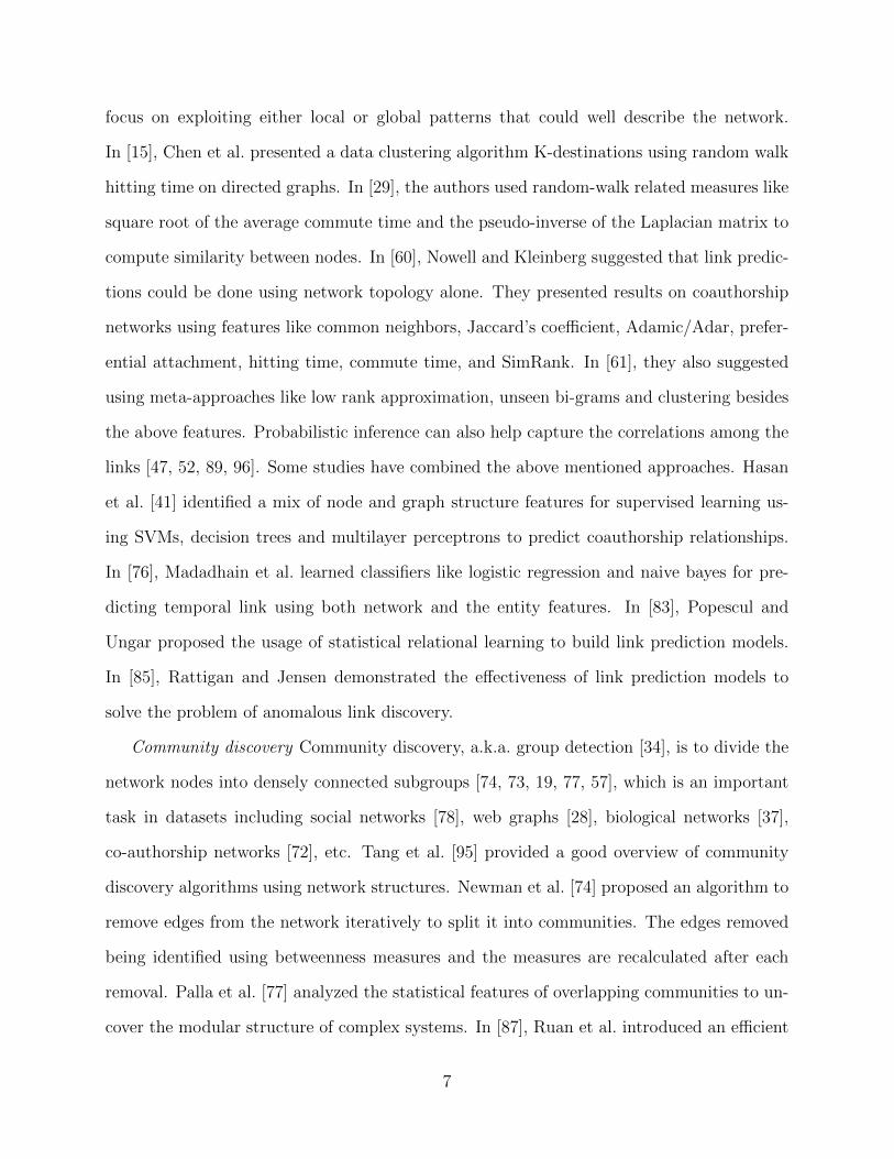
focus on exploiting either local or global patterns that could well describe the network.

In [15], Chen et al. presented a data clustering algorithm K-destinations using random walk

hitting time on directed graphs. In [29], the authors used random-walk related measures like

square root of the average commute time and the pseudo-inverse of the Laplacian matrix to

compute similarity between nodes. In [60], Nowell and Kleinberg suggested that link predic-

tions could be done using network topology alone. They presented results on coauthorship

networks using features like common neighbors, Jaccard’s coefficient, Adamic/Adar, prefer-

ential attachment, hitting time, commute time, and SimRank. In [61], they also suggested

using meta-approaches like low rank approximation, unseen bi-grams and clustering besides

the above features. Probabilistic inference can also help capture the correlations among the

links [47, 52, 89, 96]. Some studies have combined the above mentioned approaches. Hasan

et al. [41] identified a mix of node and graph structure features for supervised learning us-

ing SVMs, decision trees and multilayer perceptrons to predict coauthorship relationships.

In [76], Madadhain et al. learned classifiers like logistic regression and naive bayes for pre-

dicting temporal link using both network and the entity features. In [83], Popescul and

Ungar proposed the usage of statistical relational learning to build link prediction models.

In [85], Rattigan and Jensen demonstrated the effectiveness of link prediction models to

solve the problem of anomalous link discovery.

Community discovery Community discovery, a.k.a. group detection [34], is to divide the

network nodes into densely connected subgroups [74, 73, 19, 77, 57], which is an important

task in datasets including social networks [78], web graphs [28], biological networks [37],

co-authorship networks [72], etc. Tang et al. [95] provided a good overview of community

discovery algorithms using network structures. Newman et al. [74] proposed an algorithm to

remove edges from the network iteratively to split it into communities. The edges removed

being identified using betweenness measures and the measures are recalculated after each

removal. Palla et al. [77] analyzed the statistical features of overlapping communities to un-

cover the modular structure of complex systems. In [87], Ruan et al. introduced an efficient

7

spectral algorithm for modularity optimization to discover community structure. Nowicki

et al. [75] proposed a statistical approach to a posteriori blockmodeling to partition the ver-

tices of the graph into several latent classes where the probability distribution of the relation

between two vertices depends only on the classes to which they belong. In [113], Zhang et

al. proposed an LDA-based hierarchical Bayesian algorithm called SSN-LDA, where commu-

nities are modeled as latent variables in the graphical models and defined as distributions

over social actor space. In [112], Zhang et al. used a Gaussian distribution with inverse-

Wishart prior to model the arbitrary weights that are associated with the social interaction

occurrences. Leskovec et al. [57] studied a range of network community detection methods

originating from theoretical computer science, scientific computing, and statistical physics

in order to compare them and to understand their relative performance and the systematic

biases in the clusters they identify. Yang et al. [120] proposed a graph clustering algorithm

(similar to k-medoids) based on both structural and attribute similarities through a unified

distance measure. In [63], Long et al. proposed a probabilistic model for relational clustering

under a large number of exponential family distributions.

2.2 Text Mining in Social Media

In this section we provide an overview of the related work to text mining in social media.

We review the existing studies on topic modeling and the extension with link and spatial-

temporal information. We also survey the work related to event detection and tracking.

Topic modeling Statistical topic models can be considered as the probabilistic models for

uncovering the underlying semantic structure of a document collection based on hierarchical

Bayesian analysis of the text collection. Topic models, such as PLSA [44] and LDA [9], use

a multinomial word distribution to represent a semantic coherent topic and model the gen-

eration of the text collection with a mixture of such topics. There are also many extensions

of the traditional topic models [6, 7, 8, 58].

8

Topic modeling with links Some studies extended topic modeling with links. In [68],

Mei et al. introduced a model called NetPLSA that regularizes a statistical topic model

with a harmonic regularizer based on a graph structure in the data. In [94], Sun et al.

defined a multivariate Markov Random Field for topic distribution random variables for

each document to model the dependency relationships among documents over the network

structure. Zhou et al. [119] proposed a generative probabilistic model to discover semantic

community in social networks, but they used text information only without considering

link structure. There are several studies on generative topic models based on text and

links including Author-Topic model [93, 86], Author-Recipient-Topic model [66, 67, 79],

Group-Topic model [103], Link-PLSA-LDA [71], Block-LDA [3], Topics-on-Participations

model [115, 116]. The generation of each link in a document is modeled as a sampling from

a topic-specific distribution over documents [20, 26]. Liu et al. [62] proposed a model called

Topic-Link LDA where the membership of authors is modeled with a mixture model and

whether a link exists between two documents follows a binomial distribution parameterized

by the similarity between topic mixtures and community mixtures as well as a random factor.

Spatial topic modeling Some works studied the spatial topics from social media. Sizov [92]

proposed a framework called GeoFolk to combine text and spatial information together

to construct better algorithms for content management, retrieval, and sharing in social

media. GeoFolk modeled each region as an isolated topic and assumed the geographical

distribution of each topic is Gaussian. In [100], Wang et al. proposed a Location Aware

Topic Model to explicitly model the relationships between locations and words, where the

locations are represented by predefined location terms in the documents. Mei et al.[69]

proposed a probabilistic approach to model the subtopic themes and spatiotemporal theme

patterns simultaneously in weblogs, where the locations need to be predefined.

Temporal topic mining Some methods were proposed to mine topics from documents

associated with timestamps. Wang et al. [102] used an LDA-style topic model to capture

both the topic structure and the changes over time. Mei et al. [69] partitioned the timeline

9

into buckets and proposed a probabilistic approach to model the subtopic themes and spa-

tiotemporal theme patterns simultaneously in weblogs. Wang et al. mined correlated bursty

topic patterns from coordinated text streams in [101]. Blei and Lafferty [7] employed state

space models on the natural parameters of multinomial distributions of topics and design

a dynamic topic model to model the time evolution of stream. Iwata et al. [45] proposed

an online topic model for sequentially analyzing the time evolution of topics in document

collections, in which current topic-specific distributions over words are assumed to be gen-

erated based on the multiscale word distributions of the previous epoch. Stochastic EM

algorithm was used in the online inference process. In [114], Zhang et al. discovered different

evolving patterns of clusters, including emergence, disappearance, evolution within a corpus

and across different corpora. The problem was formulated as a series of hierarchical Dirichlet

processes by adding time dependencies to the adjacent epochs, and a cascaded Gibbs sam-

pling scheme is used to infer the model. All the existing studies on temporal topic mining

focus on the evolutionary pattern of the topics.

Event detection and tracking In [1], Allan et al. introduced the problems of event detec-

tion and tracking within a stream of broadcast news stories. To extract meaningful struc-

ture from document streams that arrive continuously over time is a fundamental problem

in text mining [50]. Kleinberg developed a formal approach for modeling the stream using

an infinite-state automaton to identify the bursts efficiently. Fung et al. [31] proposed Time

Driven Documents-partition framework to construct a feature-based event hierarchy for a

text corpus based on a given query. In [59], Li et al. proposed a probabilistic model to incor-

porate both content and time information in a unified framework to detect the retrospective

news events. In [42], He et al. used concepts from physics to model bursts as intervals of

increasing momentum, which provided a new view of bursty patterns. Besides traditional

text documents like news articles and research publications, event detection is also studied in

those new social media like Twitter and Flickr [4, 88]. Becker et al. [4] explored a variety of

techniques for learning multi-feature similarity metrics for social media documents to detect

10

events. In [88], Sakaki et al. proposed an algorithm to monitor tweets to detect real time

events such as earthquakes and typhoons. In [56], Leskovec et al. proposed a meme-tracking

approach to provide a coherent representation of the news cycle, i.e., daily rhythms in the

news media. Yang et al. [104] studied temporal patterns with online content and how the

popularity of the content grows and fades over time. These studies of event detection and

tracking mainly focus on mining temporal bursts.

2.3 Spatial-temporal Mining in Social Media

In this section we review the related work about spatial-temporal mining in geo-tagged social

media. We have reviewed other related work about spatial-temporal mining with text data

in Section 2.2.

With the development of GPS technology, several studies have been done in geo-tagged

social media mining. Amitay et al.[2] described a system called Web-a-Where for associating

geography with Web pages. Rattenbury et al.[84] proposed a Scale-structure Identification

method to extract the event and place semantics from Flickr tags based on the time and

location metadata. To enhance semantic and geographic annotation of web images on Flickr,

Cao et al.[12] used Logistic Canonical Correlation Regression (LCCR) to improve the anno-

tation by exploiting the correlation between heterogeneous features and tags. Crandall et

al. [22] predicted the locations for the photos on Flickr from the visual, textual and temporal

features. In [90], Serdyukov et al. predicted the locations for the Flickr photos by a language

model on user annotations. They extended the language model by tag-based smoothing and

cell-based smoothing. Besides mining the location information for Flickr images, blog is also

a good source to extract landmarks [46, 39, 40]. Silva et al. [23] also proposed a system

for retrieving multimedia travel stories by using location data. Some studies focused on

mining trip information based on the sequence of locations. Popescu et al. [82, 81] showed

how to extract clean trip related information from Flickr metadata. They extracted the

11

place names from Wikipedia and generated the trip by mapping the photo tags to location

names. In [18, 17], Choudhury et al. formulated trip planning as directed orienteering prob-

lem. In [64], Lu et al. used dynamic programming for trip planning. In [49], Kennedy et al.

used location, tags and visual features of the images to generate diverse and representative

images for the landmarks.

12

Chapter 3

Link Recommendation

3.1 Introduction

Social networking sites such as Facebook, Twitter, and LinkedIn have drawn much more

attention than ever before. The users not only use the social network sites to maintain

contacts with old friends, but also use the sites to find new friends with similar interests and

for business networking. Since the link among people is the underlying key concept for online

social network sites, it is not surprising that link recommendation is an essential link mining

task. First, link recommendation can help users to find potential friends, a function that

improves user experience in social networking sites and attracts more users consequently.

Compared with the usual passive ways of locating possible friends, the users on these social

networks are provided with a list of potential friends, with a simple confirmation click.

Second, link recommendation helps the social networking sites grow fast in terms of the

social linkage. A more complete social graph not only improves user involvement, but also

provides the monetary benefits associated with a wide user base such as a large publisher

network for advertisements.

Link prediction is the problem of predicting the existence of a link between two entities in

an entity relationship graph, where prediction is based on the attributes of the objects and

other observed links. Link prediction has been studied on various kinds of graphs including

metabolic pathways, protein-protein interaction, social networks, etc. These studies use

different measures such as node-wise similarity and topology-based similarity to predict

the existence of the links. In addition to these existing measures, different models have

13

been investigated for the link prediction tasks including relational Bayesian networks and

relational Markov networks. Link recommendation in social network is closely related to

link prediction, but has its own specific properties. Social network can be considered as a

graph where each node has its own attributes. Linked entities share certain similarities with

respect to attribute information associated with entities and structure information associated

with the graph. We study the problem of expressing the link relevance to incorporate both

attributes and structure in a unified and intuitive manner.

3.2 Problem Formulation

Given a social graph G (V , E), where V is the set of nodes and E is the set of edges, each

node in V represents a person in the network and each edge in E represents a link between

two person nodes. Besides the links, each person has his/her own attributes. The existence

of an edge in G represents a link relationship between the two persons.

The link recommendation task can be expressed as: Given node v in V , provide a ranked

list of nodes in V as the potential links ranked by link relevance (with the existing linked

nodes of v removed).

The following presents some intuition-based desiderata for link relevance where Alice is

more likely to form a link with Bob rather than with Carol.

1. Homophily : Two persons who share more attributes are more likely to be linked than

those who share fewer attributes. E.g., Alice and Bob both like Football and Tennis,

and Alice has no common interest with Carol.

2. Rarity : The rare attributes are likely to be more important, whereas the common

attributes are less important. E.g., only Alice and Bob love Hiking, but thousands of

people, including Alice and Carol, are interested in Football.

3. Social influence: The attributes shared by a large percentage of friends of a particular

14

person are important for predicting potential links for that person. E.g., most of the

people linked to Alice like Football, and Bob is interested in Football but Carol is not.

4. Common friendship: The more neighbors two persons share, the more likely it is that

they are linked together. E.g., Alice and Bob share over one hundred friends, but Alice

and Carol have no common friend.

5. Social closeness : The potential friends are likely to be located close to each other in

the social graph. E.g., Alice and Bob are only one step away from each other in social

graph, but Alice and Carol are five steps apart.

6. Preferential attachment : A person is more likely to link to a popular person rather

than to a person with only a few friends. E.g., Bob is very popular and has thousands

of friends, but Carol has only ten friends.

A good link candidate should satisfy the above criteria both on the attribute and structure

in social networks. In other words, the link relevance should be estimated by considering

the above intuitive rules.

3.3 Proposed Solution

3.3.1 Graph Construction

Given the original social graph G(V,E), we construct a new graph G′(V ′, E ′), augmented

based on G. Specifically, for each node in graph G, we create a corresponding node in G′,

called person node. For each edge in E in graph G, we create a corresponding edge in G′.

For each attribute a, we create an additional node in G′, called attribute node. V ′ = Vp ∪ Va

where Vp is the person node set and Va is the attribute node set. For every attribute of a

person, we create a corresponding edge between the person node and the attribute node.

15

Table 3.1: Attributes and relationships of users in a social network.

User Attributes Friends

Alice “c++”, “python” Bob, CarolBob “c++”, “c#”, “python” Alice, CarolCarol “c++”, “c#”, “perl” Alice, Bob, DaveDave “java”, “perl” Carol, EveEve “java”, “perl” Dave

Example 1 Consider a social network of five people: Alice, Bob, Carol, Dave and Eve. The

attributes and relationships of the users are shown in Table 3.1. The augmented graph G′

containing both person nodes and attribute nodes is shown in Figure 3.1.

Figure 3.1: An augmented graph with person and attribute nodes.

The edge weights in G′ are defined by the uniform weighting scheme. The weight w(a, p)

of the edge from attribute node a to person node p is defined as follows.

w(a, p) =1

|Np(a)|(3.1)

where Np(a) denotes the set of person nodes connected to attribute node a.

Given person node p, attribute node a connected to p and person node p′ connected to

node p, the edge weight w(p, a) from person node p to attribute node a and the edge weight

w(p, p′) from person node p to person node p′ are defined as follows.

16

w(p, a) =

λ

|Na(p)| if |Na(p)| > 0 and |Np(p)| > 0;

1|Na(p)| if |Na(p)| > 0 and |Np(p)| = 0;

0 otherwise.

(3.2)

w(p, p′) =

1−λ|Np(p)| if |Np(p)| > 0 and |Na(p)| > 0;

1|Np(p)| if |Np(p)| > 0 and |Na(p)| = 0;

0 otherwise.

(3.3)

where Na(p) denotes the set of the attribute nodes connected to node p, Np(p) denotes the

set of person nodes connected to node p, and λ controls the tradeoff between attribute and

structural properties. The larger λ is, the more the algorithm uses attribute properties for

link recommendation. Specifically, if λ = 1, the algorithm makes use of the attribute features

only. If λ = 0, it is based on structural properties only.

3.3.2 Algorithm Design

In order to calculate the link relevance based on the criteria in Section 3.2, we propose a

random walk based algorithm on the newly constructed graph to simulate the friendship

hunting behavior. The stationary probabilities of random walk starting from a given person

node are considered as the link relevance between the person node and the respective nodes

in the probability distribution.

Random walk process on the newly constructed graph satisfies the desiderata (provided

in the Section 3.2) for link relevance in the following ways. (1) If two persons share more

attributes, the corresponding person nodes in the graph will have more connected attribute

nodes in common. Therefore, the random walk probability from one person node to the

other via those common attribute nodes is high. (2) If one attribute is rare, there are fewer

17

outlinks for the corresponding attribute node. Therefore, the weight of each outlink is larger

and the probability of a random walk originating from a person and reaching the other

person node via this attribute node is larger. (3) If one attribute is shared by many of the

existing linked persons of the given person, the random walk will pass through the existing

linked person nodes to this attribute node. (4) If two persons share many friends, these

two person nodes have a large number of common neighbors in the graph. Therefore, the

random walk probability from one person node to the other is high. (5) If two person nodes

are close to each other in the graph, the random walk probability from one to the other is

likely to be larger than if they are far away from each other. (6) If a person is very popular

and links to many persons, there are many inlinks to the person node in the graph. For a

random person node in the graph it is easier to access a node with more inlinks.

Here, we use the random walk with restart on the augmented graph with person and

attribute nodes to calculate the link relevance for a particular person p∗.

rp = (1− α)∑

p′∈Np(p)

w(p′, p)rp′ (3.4)

+(1− α)∑

a′∈Na(p)

w(a′, p)ra′ + αr(0)p

ra = (1− α)∑

p′∈Np(p)

w(p′, a)rp′ (3.5)

where rp is the link relevance of person p with regard to p∗, i.e., the random walk probability

of person node p from person node p∗, ra is the relevance of attribute a with regard to p∗,

i.e., the random walk probability of attribute node a from person node p∗, and α is the

restart probability. r(0)p = 1 if node p refers to person p∗ and r

(0)p = 0 otherwise.

18

3.3.3 Edge Weighting

The edge weighting in the augmented graph is important to the link recommendation algo-

rithm. In Section 3.3.1, we assigned weights to each attribute uniformly. Here we propose

several edge weighting methods for the edges from person nodes to attribute nodes. The

edge weight w(p, a) from person node p to attribute node a is defined as follows.

w(p, a) =

λwp(a)∑

a′∈Na(p) wp(a′)if |Na(p)| > 0 and |Np(p)| > 0;

wp(a)∑a′∈Na(p) wp(a′)

if |Na(p)| > 0 and |Np(p)| = 0;

0 otherwise.

where wp(a) is the importance score for attribute a with regard to person p, Na(p) denotes

the set of the attribute nodes connected to node p, Np(p) denotes the set of the person nodes

connected to node p, and λ controls the tradeoff between attribute and structural properties.

Global Weighting: Instead of weighting all the attributes equally, we should attach more

weight to the more promising attributes. Here we give the definition of attribute global

importance g(a) for attribute a in social graph G(V,E) as follows.

g(a) =

∑(u,v)∈E e

auv(

na2

)na is the number of the persons that have attribute a. eauv = 1 if persons u and v both have

attribute a, eauv = 0 otherwise. The global importance score for attribute a measures the

percentage of existing links among all the possible person pairs with the attribute a. The

local importance score g(a) is used as wp(a).

Local Weighting: Instead of considering the attributes globally, we derive the local im-

portance of the attributes for the specific person based on its neighborhood. The definition

19

of attribute local importance lp(a) for attribute a with regard to person p is as follows.

lp(a) =∑

p′∈Np(p)

A(p′, a)

where Np(p) denotes the set of the person nodes connected to node p. A(p, a) = 1 if person

p has attribute a, A(p, a) = 0 otherwise. The definition demonstrates that the more the

number of friends that share the attribute, the more important the attribute is for the

person. The local importance score lp(a) is used as wp(a), so the edge weight from person p

to attribute a depends on the local importance of a with regard to p.

Mixed Weighting: Other than considering global and local importance separately, we can

combine the two together.

The first mixture method is to use linear interpolation to combine the global and local

importance together.

wp(a) = γg(a)∑

a′∈Na(p) g(a′)+ (1− γ)

lp(a)∑a′∈Na(p) lp(a

′)

where γ controls the tradeoff between the global importance score and the local importance

score.

The second mixture method is to construct attribute importance score by multiplying

global and local importance score.

wp(a) = g(a)× lp(a)

3.3.4 Attribute Ranking

Besides link recommendation, we can rank attributes with respect to a specific person by

using the proposed framework. Attribute ranking can have many potential applications.

For example, advertisements can be targeted more accurately if we know a person’s interests

20

more precisely. Furthermore, we can analyze the behavior of users of a particular category.

In the augmented graph, all the nodes including the attribute nodes have the random walk

probability. Similarly, we can rank attribute nodes based on the random walk probability in

Equation 3.5. The attributes with high ranks in our framework are those that are frequently

shared by the given person, the existing friends and the potential friends.

Instead of ranking the attributes for a single person, we can also rank the attributes

for a cluster of person nodes. For example, we can discover the most relevant interests for

all computer science graduate students. To achieve this, instead of starting random walk

from a single node, we can restart with a bundle of nodes. The equations are the same as

Equations (3.4) and (3.5) except for the definition of r(0)p . Let P be the set of the persons

to be analyzed, r(0)p = 1

|P | if node p belongs to P and r(0)p = 0 otherwise.

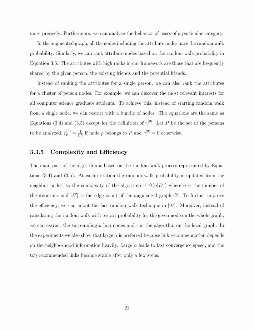
3.3.5 Complexity and Efficiency

The main part of the algorithm is based on the random walk process represented by Equa-

tions (3.4) and (3.5). At each iteration the random walk probability is updated from the

neighbor nodes, so the complexity of the algorithm is O(n|E ′|) where n is the number of

the iterations and |E ′| is the edge count of the augmented graph G′. To further improve

the efficiency, we can adopt the fast random walk technique in [97]. Moreover, instead of

calculating the random walk with restart probability for the given node on the whole graph,

we can extract the surrounding k-hop nodes and run the algorithm on the local graph. In

the experiments we also show that large α is preferred because link recommendation depends

on the neighborhood information heavily. Large α leads to fast convergence speed, and the

top recommended links become stable after only a few steps.

21

Table 3.2: Statistics of datasets.

Statistics DBLP IMDB

# Person nodes 2500 6750# Attribute nodes 11749 9851

# Average attributes per person 93.94 29.02# Average links per person 6.63 96.67

3.4 Experiment

In this section, we describe our experiments on real data sets to demonstrate the effectiveness

of our framework.

3.4.1 Datasets

DBLP. Digital Bibliography Project (DBLP) is a computer science bibliography. Authors

in the WWW conference from year 2001 to year 2008 are represented as person nodes in

our graph. For each author, we get the entire publication history. Terms in the paper titles

are considered as the attributes for the corresponding author. Co-authorship between two

authors maps to the link between their corresponding person nodes.

IMDB. The Internet Movie Database (IMDB) is an online database of information related

to movies, actors, television shows, etc. We consider all the actors and actresses who have

performed in more than ten movies (we excluded TV shows) since 2005. Movie locations

are considered as their attributes. If two persons appear in the same movie, we create a link

between the corresponding nodes.

The statistics of DBLP and IMDB data sets are listed in Table 3.2.

3.4.2 Link Recommendation Criteria

We proposed the desired criteria for link recommendation in Section 3.2. Here we show the

existence of these criteria in both data sets. (1) We sample the same number of non-linked

22

a(1) DBLP a(2) IMDB

b(1) DBLP b(2) IMDB

c(1) DBLP c(2) IMDB

d(1) DBLP d(2) IMDB

Figure 3.2: Verification of link recommendation criteria in datasets.

pairs as that of linked pairs in both data sets. As shown in Figure 3.2a, compared to the

non-linked pairs, the linked pairs are more likely to share more attributes. (2) We analyze the

correlation between the global importance of an attribute and the number of people sharing

23

the attribute. The global importance of the attribute measures the percentage of existing

links among all the possible person pairs with this attribute. The larger the global weight

is, the more predictive the attribute is for link recommendation. As shown in Figure 3.2b,

we find that the attributes of lower frequency are likely to have higher global weights. (3) If

we randomly draw a person from the linked persons, it is obvious that the selected person

is more likely to have the frequent attribute in common with these linked persons. (4)

We sample equal number of non-linked pairs and linked pairs. As shown in Figure 3.2c,

compared to the non-linked pairs, the linked pairs are more likely to share more neighbors.

(5) We construct a new graph by removing 25% linked node pairs from the original graph.

We test the distances between the removed 25% node pairs in the new graph. We sample

the same number of non-linked pairs as the removed linked node pairs in the original graph.

As shown in Figure 3.2d, compared to the non-linked pairs in the original graph, these 25%

node pairs are much closer to each other. (6) The node degree determines number of persons

a particular person is linked to. A popular person is more likely to be highly linked.

3.4.3 Accuracy Metrics and Baseline

Accuracy Metrics. We remove some of the edges in the graph and recommend the links

based on the pruned graph. Four-fold cross validation is used on both of the data sets in

the experiment: randomly divide the set of links in the social graph into four partitions, use

one partition for testing, and retain the links in other partitions. We randomly sample 100

people and recommend the top-k links for each person. We use precision, recall and mean

reciprocal rank (MRR) for reporting accuracy. P@k = 1|S|∑

p∈S Pk(p) where S is the set of

sampled person nodes, Pk(p) = Nk(p)k

and Nk(p) is the number of the truly linked persons

in the top-k list of person p. recall = 1|S|∑

p∈S recall(p) where recall(p) = |Fp∩Rp||Fp| (recall is

measured on the top-50 results). Fp is the truly linked person set of person p and Rp is the

set of recommended linked persons of person p. MRR = 1|S|∑

p∈S1

rankpwhere rankp is the

rank of the first correctly recommended link of person p.

24

Baseline methods. To demonstrate the effectiveness of our method, we compare our

method with the other methods based on the attribute and structure.

• Random: Random selection.

• SimAttr: Cosine similarity based on the attribute space.

• WeightedSimAttr: Cosine similarity based on the attribute space using global impor-

tance as the attribute weight.

• ShortestDistance: The length of the shortest path.

• CommonNeighbors: score(x, y) = |Γ(x) ∩ Γ(y)|. Γ(x) is the set of neighbors of x in

graph G.

• Jaccard: score(x, y) = |Γ(x) ∩ Γ(y)|/|Γ(x) ∪ Γ(y)|.

• Adamic/Adar: score(x, y) =∑

z∈Γ(x)∩Γ(y)1

log |Γ(z)| .

• PrefAttach: score(x, y) = |Γ(x)| · |Γ(y)|.

• Katz: score(x, y) =∑

l=1..∞ βl · |path<l>x,y |, where β is the damping factor and path<l>x,y

is the set of all length-l paths from x to y. We consider the paths with length no more

than 3.

To compare our method with the supervised learning methods, we use Support Vector

Machine (SVM) on a combination of attribute and structure features. Specifically, we use

the promising features, including SimAttr, WeightedSimAttr, CommonNeighbors, Jaccard,

Adamic/Adar and Katz, for the training. Here we use the LIBSVM toolkit1. Both linear

kernel and Radial Basis Function (RBF) kernel are tested. We use SVM Linear to denote

the SVM method using linear kernel and SVM RBF to denote the SVM method using RBF

kernel in Tables 3.3 and 3.4.

1http://www.csie.ntu.edu.tw/˜cjlin/libsvm

25

Table 3.3: Comparison of the methods in DBLP dataset.

P@1 P@5 P@10 P@20 P@50 Recall MRR

Random 0.000 0.000 0.001 0.002 0.002 0.024 0.004PrefAttach 0.023 0.015 0.015 0.011 0.009 0.119 0.057ShortestDistance 0.075 0.066 0.060 0.054 0.038 0.705 0.183SimAttr 0.363 0.146 0.095 0.060 0.033 0.579 0.448WeightedSimAttr 0.618 0.281 0.172 0.097 0.045 0.738 0.674CommonNeighbors 0.578 0.273 0.171 0.103 0.051 0.816 0.665Jaccard 0.563 0.272 0.171 0.105 0.050 0.800 0.654Adamic/Adar 0.628 0.299 0.187 0.109 0.051 0.823 0.713Katz β = 0.05 0.575 0.265 0.175 0.104 0.051 0.820 0.664Katz β = 0.005 0.573 0.268 0.176 0.105 0.051 0.819 0.664Katz β = 0.0005 0.573 0.267 0.176 0.104 0.051 0.820 0.663SVM RBF 0.543 0.290 0.188 0.110 0.051 0.825 0.664SVM Linear 0.623 0.299 0.186 0.110 0.051 0.821 0.707RW Uniform: λ = 0.6, α = 0.9 0.700 0.347 0.214 0.123 0.056 0.907 0.777RW Global: λ = 0.6, α = 0.7 0.735 0.353 0.218 0.124 0.055 0.891 0.795RW Local: λ = 0.7, α = 0.9 0.723 0.335 0.199 0.114 0.052 0.859 0.788RW MIX: λ = 0.6, α = 0.9, γ = 0.6 0.748 0.361 0.219 0.122 0.055 0.881 0.806RW MIX2: λ = 0.5, α = 0.9 0.720 0.346 0.206 0.119 0.054 0.873 0.787

We use RW Uniform to denote our method using uniform weighting scheme, RW Global

to denote our method using global edge weighting, RW Local to denote our method using

local edge weighting, RW MIX to denote our method using mixed weighting of global and

local importance by linear interpolation, and RW MIX2 to denote our method using mixed

weighting by multiplication of global and local attribute importance.

3.4.4 Methods Comparison

Here we compare accuracy of link recommendation using different methods on the DBLP and

IMDB data sets. The results are listed in Tables 3.3 and 3.4. Random method performs the

worst as expected. Since there are so many person nodes in the graph, it is almost impossible

to recommend the correct links by random selection. PrefAttach and ShortestDistance

perform poorly in both data sets.

Structure-based measures other than ShortestDistance perform well for both data sets.

This indicates that the graph structure plays a crucial role in link recommendation. Com-

pared with DBLP, precision and MRR in IMDB are much higher, but recall is lower. The

26

Table 3.4: Comparison of the methods in IMDB dataset.

Method P@1 P@5 P@10 P@20 P@50 Recall MRR

Random 0.003 0.004 0.003 0.002 0.003 0.008 0.012PrefAttach 0.048 0.028 0.023 0.022 0.017 0.027 0.092ShortestDistance 0.003 0.008 0.007 0.008 0.009 0.032 0.033SimAttr 0.663 0.536 0.424 0.291 0.159 0.361 0.738WeightedSimAttr 0.818 0.682 0.565 0.414 0.218 0.476 0.852CommonNeighbors 0.848 0.740 0.653 0.504 0.287 0.639 0.900Jaccard 0.878 0.771 0.684 0.547 0.315 0.669 0.913Adamic/Adar 0.845 0.757 0.670 0.518 0.299 0.666 0.899Katz β = 0.05 0.420 0.367 0.334 0.259 0.155 0.356 0.531Katz β = 0.005 0.743 0.671 0.584 0.445 0.254 0.576 0.833Katz β = 0.0005 0.818 0.716 0.634 0.485 0.277 0.606 0.878SVM RBF 0.745 0.696 0.634 0.515 0.305 0.677 0.823SVM Linear 0.855 0.759 0.679 0.553 0.331 0.712 0.900RW Uniform: λ = 0.1, α = 0.8 0.878 0.766 0.683 0.554 0.333 0.724 0.917RW Global: λ = 0.2, α = 0.9 0.910 0.799 0.694 0.551 0.335 0.723 0.938RW Local: λ = 0.4, α = 0.9 0.945 0.814 0.703 0.543 0.316 0.694 0.961RW MIX: λ = 0.4, α = 0.9, γ = 0.1 0.943 0.813 0.704 0.543 0.318 0.699 0.959RW MIX2: λ = 0.2, α = 0.9 0.953 0.818 0.706 0.559 0.335 0.723 0.965

reason is that on average there are much more links per person in IMDB (96.67) than in

DBLP (6.63). The more the links, the more likely we can get correct link recommendations

in the top results. Furthermore, dense graph structure makes structure-based measures more

expressive.

Attribute-based measures (especially WeightedSimAttr) perform fairly well in both DBLP

and IMDB. Accuracy achieved by WeightedSimAttr is comparable to that achieved by

structure-based measures. It indicates that attribute information complements to the struc-

ture features for link recommendation in these two data sets. WeightedSimAttr uses the

global importance as the attribute weight, whereas SimAttr weighs all the attributes equally.

The effectiveness of global importance score helps WeightedSimAttr to be more accurate than

SimAttr.

Supervised learning methods SVM RBF and SVM Linear perform well, but cannot beat

the best baseline measure in precision at top in both of the data sets. It shows that directly

combining attribute and structure features using supervised learning technique may not

lead to good results. Although SVM makes use of both attribute and structure properties,

27

it does not take into account the semantics behind the link recommendation criteria when

computing the model.

Compared with the baseline methods, our methods perform significantly better in both

DBLP and IMDB. In DBLP, RW MIX has the best precision (74.75% precision at 1, 36.05%

precision at 5 and 21.87% precision at 10) and the best MRR (80.58%), while RW Uniform

has the best recall (90.68%). In IMDB, RW MIX2 has the best precision (95.25% precision

at 1, 81.80% precision at 5, 70.58% precision at 10) and the best MRR (96.48%), while

RW Uniform has the best recall (72.43%). Global and local weighting methods reinforce the

link recommendation criteria. Hence, RW Global, RW Local, RW MIX and RW MIX2 can

beat RW Uniform in terms of precision at top and MRR. In DBLP, RW Global performs

better than RW Local, because the global attributes (keywords) play an important role in

link recommendation compared to very specific attributes shared with coauthors. In IMDB,

RW Local performs better than RW Global, which suggests that the movie locations of the

partners has a significant influence on actors. Also, in DBLP, RW MIX can beat both

RW Global and RW Local, whereas in IMDB RW MIX2 can outperform RW Global and

RW Local. Note that RW MIX may not always provide accuracy between that of RW Global

and RW Local because some people have high local influence while some others have high

global influence.

3.4.5 Parameter Setting

In our link recommendation framework, there are two parameters λ and α. We discuss

how to set both parameters and how the parameter settings affect the link recommendation

results.

Parameter setting. Different data sets may lead to different optimal λ and α. We

obtain the best values of these parameters by performing a grid search over ranges of val-

ues for these parameters and measuring accuracy on the validation set for each of these

configuration settings.

28

Table 3.5: Recommended Persons in DBLP dataset.Rakesh Agrawal Ricardo A. Baeza-Yates Jon M. Kleinberg Ravi Kumar Gerhard Weikum

Roberto J. Bayardo Jr. Nivio Ziviani Christos Faloutsos Andrew Tomkins Fabian M. Suchanek

Ramakrishnan Srikant Carlos Castillo Jure Leskovec D. Sivakumar Gjergji Kasneci

Jerry Kiernan Vassilis Plachouras Prabhakar Raghavan Andrei Z. Broder Klaus Berberich

Christos Faloutsos Alvaro R. Pereira Jr. Andrew Tomkins Sridhar Rajagopalan Srikanta J. Bedathur

Yirong Xu Massimiliano Ciaramita Ravi Kumar Ziv Bar-Yossef Michalis Vazirgiannis

Daniel Gruhl Aristides Gionis Cynthia Dwork Prabhakar Raghavan Stefano Ceri

Gerhard Weikum Barbara Poblete Lars Backstrom Jasmine Novak Timos K. Sellis

Timos K. Sellis Gleb Skobeltsyn Ronald Fagin Jon M. Kleinberg Jennifer Widom

Serge Abiteboul Ravi Kumar Sridhar Rajagopalan Christopher Olston Hector Garcia-Molina

Sridhar Rajagopalan Massimo Santini Deepayan Chakrabarti Anirban Dasgupta Francois Bry

Rafael Gonzalez-Cabero Sebastiano Vigna Uriel Feige Daniel Gruhl Frank Leymann

Asuncion Gomez-Perez Qiang Yang D. Sivakumar Uriel Feige Wolfgang Nejdl

*Names in Italics font represent true positives.

Effect of λ setting. λ controls the tradeoff between attribute and structural properties.

Higher value of λ implies that the algorithm gives more importance to the attribute features

than structure features. We find the optimal λ is 0.6 in DBLP and 0.2 in IMDB, and

the combination of attribute and structural features is much better than using attribute or

structure properties individually.

Effect of α setting. α is the restart probability of random walks. Random walk with

restart is quite popular in applications like personalized search and query suggestion. In our

link recommendation setting, large α provides more accurate link recommendation, unlike

low α in traditional applications. In personalized search, random walks are used to discover

relevant entities spread out in the entire graph, so a small α is favorable in those cases.

However, in link recommendation task, we are more focused on the local neighborhood

information, so a large α is more reasonable. We find that α = 0.9 provides the best result.

Besides high accuracy, large α makes the algorithm converge faster.

3.4.6 Case Study

We select several well known researchers and show the recommended persons in Table 3.5

as well as top-ranked keywords for each person in Table 3.6. Since we partition the links

into four partitions, the recommended persons in Table 3.5 are selected from top-3 results

29

Table 3.6: Attribute Ranking in DBLP dataset.

Rakesh Soumen Ricardo A. Ravi Jon M. ChengXiang Jure GerhardAgrawal Chakrabarti Baeza-Yates Kumar Kleinberg Zhai Leskovec Weikum

mining search search search networks retrieval networks xmldatabase mining retrieval networks algorithms information graphs searchdatabases information information information search search information information

information algorithms query algorithms social language graph databasesystems dynamic semantic time information mining network peersearch learning xml semantic network models social management

applications databases analysis analysis analysis model evolution queryxml structure model graph systems learning learning systems

semantic queries searching systems problem analysis search semanticsystem networks matching efficient graph modeling marketing efficient

in each partition obtained by applying our framework using global weighting strategy. The

top-ranked keywords in Table 3.6 are selected by applying our framework using uniform

weighting on the complete coauthorship graph without partitioning.

3.5 Conclusions and Future Work

We propose a framework for link recommendation based on attribute and structural prop-

erties in a social network. We first enumerate the desired criteria for link recommendation.

To calculate the link relevance that satisfies those criteria, we augment the social graph with

attributes as additional nodes and use a random walk algorithm on the augmented graph.

Both global and local attribute information can be leveraged into the framework by influ-

encing edge weights. Besides link recommendation, our framework can be easily adapted to

provide attribute ranking as well.

Our framework can be further improved in several aspects. First, attributes may be

correlated with each other. The framework should automatically identify such semantic cor-

relations and handle it properly for link recommendation. Second, the algorithm currently

adds a new attribute node for every value of categorical attributes. Handling numeric at-

tributes would require tuning to appropriate level of discretization. We also plan to test the

effectiveness of our method on friendship networks like Facebook.

30

Chapter 4

Latent Geographical Topic Analysis

4.1 Introduction

With the popularity of low-cost GPS chips and smart phones, geographical records have

become prevalent on the Web. A geographical record is usually denoted by a two dimensional

vector, latitude and longitude, representing a unique location on the Earth. There are several

popular ways to obtain geographical records on the Web:

1. Advanced cameras with GPS receivers could record GPS locations when the photos

were taken. When users upload these photos on the Web, we can get the geographical

records from the digital photo files.

2. Some applications including Google Earth and Flickr provide interfaces for users to

specify a location on the world map. Such a location can be treated as a geographical

record in a reasonable resolution.

3. People can record their locations by GPS functions in their smart phones. Popular so-

cial networking websites, including Facebook, Twitter, Foursquare and Dopplr, provide

services for their users to publish such geographical information.

In the above three scenarios, GPS records are provided together with different docu-

ments including tags, user posts, etc. We name those documents with GPS records as

GPS-associated documents. The amount of GPS-associated documents is increasing dra-

matically. For example, Flickr hosts more than 100 million photos associated with tags

31

and GPS locations. The large amount of GPS-associated documents makes it possible to

analyze the geographical characteristics of different subjects. For example, by analyzing

the geographical distribution of food and festivals, we can compare the cultural differences

around the world. We can also explore the hot topics regarding the candidates in presidential

election in different places. Moreover, we can compare the popularity of specific products

in different regions and help make the marketing strategy. The geographical characteristics

of these topics call for effective approaches to study the GPS-associated documents on the

Web.

In recent years, some studies have been conducted on GPS-associated documents in-

cluding organizing geo-tagged photos [22] and searching large geographical datasets [49].

However, none of them addressed the following two needs in analyzing GPS-associated doc-

uments.

• Discovering different topics of interests those are coherent in geographical regions. Ad-

ministrative divisions such as countries and states can be used as regions to discover

topics. However, we are more interested in different region segmentations correspond-

ing to different topics. For example, a city can be grouped into different sub-regions in

terms of architecture or entertainment characteristics; a country might be separated

into regions according to landscapes like desert, beach and mountain. Unfortunately,

existing studies either overlook the differences across geographical regions or employ

country/state as the fixed configuration.

• Comparing several topics across different geographical locations. It is often more inter-

esting to compare several topics than to analyze a single topic. For example, people

would like to know which products are more popular in different regions, and sociolo-

gists may want to know the cultural differences across different areas. With the help

of GPS-associated documents, we can map topics of interests into their geographical

distributions. None of the previous work addressed this problem and we aim to develop

32

an effective method to compute such comparison.

We propose three different models for geographical topic discovery and comparison. First,

we introduce a location-driven model, where we cluster GPS-associated documents based on

their locations and make each document cluster as one topic. The location-driven model

works if there exist apparent location clusters. Second, we introduce a text-driven model,

which discovers topics based on topic modeling with regularization by spatial information.

The text-driven model can discover geographical topics if the regularizer is carefully selected.

However, it cannot get the topic distribution in different locations for topic comparison, since

locations are only used for regularization instead of being incorporated into the generative

process. Third, considering the facts that a good geographical configuration benefits the

estimation of topics, and that a good topic model helps identify the meaningful geographical

segmentation, we build a unified model for both topic discovery and comparison. We propose

a novel location-text joint model called LGTA (Latent Geographical Topic Analysis), which

combines geographical clustering and topic modeling into one framework. Not only can we

discover the geographical topics of high quality, but also can estimate the topic distribution

in different geographical locations for topic comparison.

4.2 Problem Formulation

In this section, we define the problem of geographical topic discovery and comparison. The

notations that we used are listed in Table 4.1.

Definition 1. A GPS-associated document is a text document associated with a GPS

location. Formally, document d contains a set of words wd, where the words are from

vocabulary set V . ld = (xd, yd) is the location of document d where xd and yd are longitude

and latitude respectively. One example of a GPS-associated document can be a set of tags

for a geo-tagged photo in Flickr, where the location is the GPS location where the photo was

33

Table 4.1: Notations used in problem formulation.

Symbol Description

V Vocabulary (word set), w is a word in VD Document collectiond A document d that consists of words and GPS location

wd The text of document dld The GPS location of document dZ The topic set, z is a topic in Zθ The word distribution set for Z, i.e., {θz}z∈Z

taken. Another example can be a tweet in Twitter, where the location is the GPS location

from the smart phone.

Definition 2. A geographical topic is a spatially coherent meaningful theme. In other

words, the words that are often close in space are clustered in a topic. We give two geo-

graphical topic examples as follows.

Example 1. Given a collection of geo-tagged photos related to festival with tags and

locations in Flickr, the desired geographical topics are the festivals in different areas, such

as Cherry Blossom Festival in Washington DC and South by Southwest Festival in Austin,

etc.

Example 2. Given a collection of geo-tagged photos related to landscape with tags and

locations in Flickr, the desired geographical topics are landscape categories that are spatially

coherent, such as coast, desert, mountain, etc.

We study the problem of geographical topic discovery and comparison. Given a collection

of GPS-associated documents, we would like to discover the geographical topics. We would

also like to compare the topics in different geographical locations. Here we give an example

of geographical topic discovery and comparison.

Example 3. Given a collection of geo-tagged photos related to food with tags and loca-

tions in Flickr, we would like to discover the geographical topics, i.e., what people eat in

34

different areas. After we discover the food preferences, we would like to compare the food

preference distributions in different geographical locations.

To support topic comparison in different locations, we define the topic distribution in

geographical location as follows.

Definition 3. A topic distribution in geographical location is the conditional dis-

tribution of topics given a specific location. Formally, p(z|l) is the probability of topic z

given location l = (x, y) where x is longitude and y is latitude, s.t.,∑

z∈Z p(z|l) = 1. From

p(z|l), we can know which topics are popular in location l.

The problem of geographical topic discovery and comparison is formulated as

follows. Given a collection of GPS-associated documents D and the number of topics K,

we would like to discover K geographical topics, i.e., θ = {θz}z∈Z where Z is the topic

set and a geographical topic z is represented by a word distribution θz = {p(w|z)}w∈V s.t.∑w∈V p(w|z) = 1. Along with the discovered geographical topics, we also would like to know

the topic distribution in different geographical locations for topic comparison, i.e., p(z|l) for

all z ∈ Z in location l as in Definition 3. In the next sections, we will present three different

models for solving this problem.

4.3 Location-driven Model

In the location-driven model, we simply cluster the documents based on their locations.

Each document cluster corresponds to one topic. p(z|d) is the probability of topic z given

document d from the location clustering result. We then estimate the word distribution θz

for topic z by p(w|z) ∝∑

d∈D p(w|d)p(d|z), where p(d|z) is obtained from p(z|d) by Bayes’

theorem. In Festival dataset in Example 1, after we cluster the photos according to their

locations, those photos close to each other are merged into the same cluster. And then we

can generate the geographical topics (i.e., festival descriptions for each region) based on tags

in each cluster.

35

To cluster objects in 2-D space, we can use partition-based clustering like KMeans,

density-based clustering like Meanshift [21] and DBScan [27], and mixture model based

clustering. After we get the word distribution θz for topic z ∈ Z based on the clustering

result, we would like to know the topic distribution in geographical location p(z|l) for topic

comparison. Therefore, we prefer a generative model for location clustering because we can

get the estimation of p(l|z). p(z|l) can be obtained by Bayes’ theorem from p(l|z). A popular

generative model is Gaussian Mixture Model (GMM). In GMM, we assume that each cluster

is mathematically represented by a Gaussian distribution and the entire data set is modeled

by a mixture of Gaussian distributions.

Although the location-driven model is straightforward, it is likely to fail if the document

locations do not have good cluster patterns. A geographical topic may be from several

different areas and these areas may not be close to each other. For example, in Landscape

dataset in Example 2, there are no apparent location clusters; mountains exist in different

areas and some are distant from each other. Therefore, the location-driven model fails in

Landscape dataset as shown in the experiment in Section 4.6.2.

4.4 Text-driven Model

In the text-driven model, we discover the geographical topics based on topic modeling. To

incorporate location information, we can use the idea of NetPLSA [68] to regularize topic

modeling. PLSA [44] models the probability of each co-occurrence of words and documents

as a mixture of conditionally independent multinomial distributions. NetPLSA regularizes

PLSA with a harmonic regularizer based on a graph structure in the data. In our case,

the nodes of the graph are documents and the edge weights are defined as the closeness in

location between two documents. Therefore, documents that are close in location would be

assumed to have similar topic distributions.

36

The objective function that NetPLSA aims to minimize is as follows.

L(D) = −(1− λ)∑d∈D

∑w∈V

c(w, d) log∑z∈Z

p(w|z)p(z|d)

+λ

2

∑(u,v)∈E

w(u, v)∑z∈Z

(p(z|du)− p(z|dv))2 (4.1)

where c(w, d) is the count of word w in document d and w(u, v) is the closeness of document

du and dv. p(w|z) is the word distribution of topic z and p(z|d) is the topic distribution of

document d. λ controls the regularization strength.

With the guidance of text information, the text-driven model may discover geographical

topics that are missed by the location-driven model. However, there are still several problems

in the text-driven model. First, we can only get the word distribution of geographical topics

θz for z ∈ Z, but we cannot get the topic distribution of geographical locations in Definition 3,

which is important for geographical topic comparison. In text-driven model we cannot know

p(z|l) because location is only used for regularization instead of being modeled in the topic

generative process. Second, it is difficult to define the document closeness measure used in

regularization. For example, in Food data set in Example 3, some food preferences exist

only in some small regions, while some others exist throughout the continent. It is difficult

to choose the closeness measure in this case.

4.5 Location-text Joint Model

In this section, we propose a novel location-text joint model called LGTA (Latent Geograph-

ical Topic Analysis), which combines geographical clustering and topic modeling into one

framework.

37

Table 4.2: Notations used in LGTA framework.

Symbol Description

R The region set, r is a region in Rφ The topic distribution set for R, i.e., {φr}r∈Rµ The mean vector set for R, i.e., {µr}r∈RΣ The covariance matrix set for R, i.e., {Σr}r∈Rα The region importance weights

4.5.1 General Idea

To discover geographical topics, we need a model to encode the spatial structure of words.

The words that are close in space are likely to be clustered into the same geographical topic.

In order to capture this property, we assume there are a set of regions. The topics are

generated from regions instead of documents. If two words are close to each other in space,

they are more likely to belong to the same region. If two words are from the same region,

they are more likely to be clustered into the same topic. In Festival dataset in Example 1,

the regions can be the areas in different cities, so the discovered geographical topics are

different festivals. In Landscape data set in Example 2, the regions can be different areas

such as the long strips along the coast and the areas in the mountains, so the discovered

geographical topics are different landscapes. In Food data set in Example 3, the regions

can be different areas that people live together, so the discovered geographical topics are

different food preferences. We would like to design a model that can identify these regions

as well as discover the geographical topics.

4.5.2 Latent Geographical Topic Analysis

In this section, we introduce our LGTA framework for geographical topic discovery and

comparison. The notations used in the framework are listed in Table 4.2.

38

Discovering geographical topics

We would like to discover K geographical topics. The word distribution set of all the topics is

denoted as θ, i.e., {θz}z∈Z . Let us assume there are N regions and denote the region set as R.

We assume that the geographical distribution of each region is Gaussian, parameterized as

(µ,Σ) = {(µr,Σr)}r∈R where µr and Σr are the mean vector and covariance matrix of region

r. α is a weight distribution over all the regions. p(r|α) indicates the weight of region r and∑r∈R p(r|α) = 1. Since topics are generated from regions, we use φ = {φr}r∈R to indicate

topic distributions for all the regions. φr = {p(z|r)}z∈Z where p(z|r) is the probability of

topic z given region r.∑

z∈Z p(z|r) = 1 for each r.

In our model, topics are generated from regions instead of documents and the geograph-

ical distribution of each region follows a Gaussian distribution. The words that are close in

space are more likely to belong to the same region, so they are more likely to be clustered

into the same topic. The generative procedure of the model is described as follows.

To generate a geographical document d in collection D:

1. Sample a region r from the discrete distribution of region importance α, r ∼ Discrete(α).

2. Sample location ld from Gaussian distribution of µr and Σr.

p(ld|µr,Σr) =1

2π√|Σr|

exp(−(ld − µr)TΣ−1

r (ld − µr)2

) (4.2)

3. To generate each word in document d:

(a) Sample a topic z from multinomial φr.

(b) Sample a word w from multinomial θz.

Instead of aligning each topic with a single region, each topic in our model can be related

to several regions. Therefore, our model can handle topics with complex shapes. Our model

identifies the regions considering both location and text information. Meanwhile, it discovers

39

the geographical topics according to the identified geographical regions. Let us denote all

parameters by Ψ = {θ, α, φ, µ,Σ}. Given the data collection {(wd, ld)}d∈D where wd is the

text of document d and ld is the location of document d, the log-likelihood of the collection

given Ψ is as follows.

L(Ψ;D) = log p(D|Ψ)

= log∏d∈D

p(wd, ld|Ψ) (4.3)

In Section 4.5.3, we show how to estimate all the parameters using an EM algorithm.

Comparing geographical topics

To compare the topics in different geographical locations, we need to get p(z|l) in Definition 3

for all topics z ∈ Z given location l = (x, y) where x is longitude and y is latitude. Given

the estimated Ψ, we first estimate the density of location l given topic z.

p(l|z,Ψ) =∑r∈R

p(l|r,Ψ)p(r|z,Ψ)

=∑r∈R

p(l|µr,Σr)p(z|r)p(r|α)

p(z|Ψ)(4.4)

where p(z|Ψ) =∑

r∈R p(z|r)p(r|α) and p(l|µr,Σr) is based on Equation 4.2.

After we get p(l|z,Ψ), we can get p(z|l,Ψ) according to Bayes’ theorem.

p(z|l,Ψ) ∝ p(l|z,Ψ)p(z|Ψ)

∝∑r∈R

p(l|µr,Σr)p(z|r)p(r|α) (4.5)

40

4.5.3 Parameter Estimation

In order to estimate parameters Ψ = {θ, α, φ, µ,Σ} in Equation 4.3, we use maximum likeli-

hood estimation. Specifically, we use Expectation Maximization(EM) algorithm to solve the

problem, which iteratively computes a local maximum of likelihood. Let us denote rd as the

region of document d. We introduce the hidden variable p(r|d,Ψ), which is the probability of

rd = r given document d and Ψ. In the E-step, it computes the expectation of the complete

likelihood Q(Ψ|Ψ(t)), where Ψ(t) is the value of Ψ estimated in iteration t. In the M-step, it

finds the estimation Ψ(t+1) that maximizes the expectation of the complete likelihood.

In the E-step, p(r|d,Ψ(t)) is updated according to Bayes formulas as in Equation 4.6.

p(r|d,Ψ(t)) =p(t)(r|α)p(wd, ld|r,Ψ(t))∑

r′∈R p(t)(r′|α)p(wd, ld|r′,Ψ(t))

(4.6)

where p(wd, ld|r,Ψ(t)) is calculated as follows.

p(wd, ld|r,Ψ(t)) = p(wd|r,Ψ(t))p(ld|r,Ψ(t)) (4.7)

where p(ld|r,Ψ(t)) = p(ld|µ(t)r ,Σ

(t)r ) is defined as Gaussian distribution in Equation 4.2 and

p(wd|r,Ψ(t)) is multinomial distribution for the words in document d in terms of probability

p(w|r,Ψ(t)).

p(wd|r,Ψ(t)) ∝∏w∈wd

p(w|r,Ψ(t))c(w,d) (4.8)

where c(d, w) is the count of word w in document d.

We assume that the words in each region are generated from a mixture of a background

model and the region-based topic models. The purpose of using a background model is

to make the topics concentrated more on more discriminative words, which leads to more

41

informative models [111].

p(w|r,Ψ(t)) = λBp(w|B) + (1− λB)∑z∈Z

p(t)(w|z)p(t)(z|r) (4.9)

p(t)(w|z) is from θ(t), and p(t)(z|r) is from φ(t). p(w|B) is the background model, which we

set as follows.

p(w|B) =

∑d∈D c(w, d)∑

w∈V∑

d∈D c(w, d)(4.10)

In the M-step, we find the estimation Ψ(t+1) that maximizes the expectation of the

complete likelihood Q(Ψ|Ψ(t)) using the following updating formulas.

p(t+1)(r|α) =

∑d∈D p(r|d,Ψ(t))

|D|(4.11)

µ(t+1)r =

∑d∈D p(r|d,Ψ(t))ld∑d∈D p(r|d,Ψ(t))

(4.12)

Σ(t+1)r =

∑d∈D p(r|d,Ψ(t))(ld − µ(t)

r )(ld − µ(t)r )T∑

d∈D p(r|d,Ψ(t))(4.13)

In order to get updated θ(t+1) and φ(t+1) in the M-step, we use another EM algorithm

to estimate them. We define the hidden variable ϕ(w, r, z), which corresponds to the events

that word w in region r is from topic z. The relevant EM updating process is as follows.

ϕ(w, r, z)← (1− λB)p(w|z)p(z|r)λBp(w|B) + (1− λB)

∑r∈R p(w|z)p(z|r)

(4.14)

p(z|r)←∑

d∈D∑

w∈V c(w, d)p(r|d,Ψ(t))ϕ(w, r, z)∑z′∈Z

∑d∈D

∑w∈V c(w, d)p(r|d,Ψ(t))ϕ(w, r, z′)

(4.15)

p(w|z)←∑

r∈R∑

d∈D c(w, d)p(r|d,Ψ(t))ϕ(w, r, z)∑w′∈V

∑r∈R∑

d∈D c(w′, d)p(r|d,Ψ(t))ϕ(w′, r, z)

(4.16)

θ and φ obtained from the above EM steps are considered as θ(t+1) and φ(t+1).

42

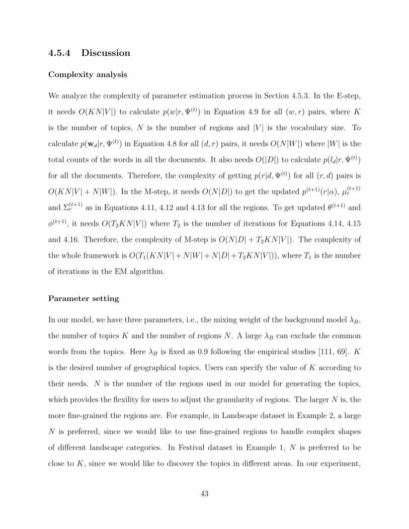
4.5.4 Discussion

Complexity analysis

We analyze the complexity of parameter estimation process in Section 4.5.3. In the E-step,

it needs O(KN |V |) to calculate p(w|r,Ψ(t)) in Equation 4.9 for all (w, r) pairs, where K

is the number of topics, N is the number of regions and |V | is the vocabulary size. To

calculate p(wd|r,Ψ(t)) in Equation 4.8 for all (d, r) pairs, it needs O(N |W |) where |W | is the

total counts of the words in all the documents. It also needs O(|D|) to calculate p(ld|r,Ψ(t))

for all the documents. Therefore, the complexity of getting p(r|d,Ψ(t)) for all (r, d) pairs is

O(KN |V |+N |W |). In the M-step, it needs O(N |D|) to get the updated p(t+1)(r|α), µ(t+1)r

and Σ(t+1)r as in Equations 4.11, 4.12 and 4.13 for all the regions. To get updated θ(t+1) and

φ(t+1), it needs O(T2KN |V |) where T2 is the number of iterations for Equations 4.14, 4.15

and 4.16. Therefore, the complexity of M-step is O(N |D| + T2KN |V |). The complexity of

the whole framework is O(T1(KN |V |+N |W |+N |D|+T2KN |V |)), where T1 is the number

of iterations in the EM algorithm.

Parameter setting

In our model, we have three parameters, i.e., the mixing weight of the background model λB,

the number of topics K and the number of regions N . A large λB can exclude the common

words from the topics. Here λB is fixed as 0.9 following the empirical studies [111, 69]. K

is the desired number of geographical topics. Users can specify the value of K according to

their needs. N is the number of the regions used in our model for generating the topics,

which provides the flexility for users to adjust the granularity of regions. The larger N is, the

more fine-grained the regions are. For example, in Landscape dataset in Example 2, a large

N is preferred, since we would like to use fine-grained regions to handle complex shapes

of different landscape categories. In Festival dataset in Example 1, N is preferred to be

close to K, since we would like to discover the topics in different areas. In our experiment,

43

small changes of N yield similar results. When the parameters are unknown, Schwarz’s

Bayesian information criterion (BIC) provides an efficient way to select the parameters. The

BIC measure includes two parts: the log-likelihood and the model complexity. The first part

characterizes the fitness over the observations, while the second is determined by the number

of parameters. In practice we can train models with different parameters, and compare their

BIC values. The model with the lowest value will be selected as the final model.

Topic guidance in comparison

We can add some guidance in the framework to make the discovered geographical topics

aligned with our needs for topic comparison. For example, in Food data set, we would like

to compare the geographical distribution of Chinese food and Italian food, we can add some

prior knowledge in two topics and guide one topic to be related to Chinese food and the other

to be related to Italian food. Specifically, we define a conjugate prior (i.e., Dirichlet prior) on

each multinomial topic distribution. Let us denote the Dirichlet prior σz for topic z. σz(w)

can be interpreted as the corresponding pseudo counts for word w when we estimate the

topic distribution p(w|z). With this conjugate prior, we can use the Maximum a Posteriori

(MAP) estimator for parameter estimation, which can be computed using the same EM

algorithm except that we would replace Equation 4.16 with the following formula:

p(w|z)←∑

d∈D c(w, d)p(r|d,Ψ(t))ϕ(w, r, z) + σz(w)∑w′∈V

∑d∈D(c(w′, d)p(r|d,Ψ(t))ϕ(w′, r, z) + σz(w′))

(4.17)

Comparison with GeoFolk

In [92], Sizov proposed a novel model named GeoFolk to combine the semantics of text feature

and spatial knowledge. Sizov shows that GeoFolk works better than text-only analysis in tag

recommendation, content classification and clustering. However, GeoFolk is not suitable for

region clustering due to two facts: First, GeoFolk models each region as an isolated topic and

thus fails to find the common topics in different geographical sites. Second, GeoFolk assumes

44

the geographical distribution of each topic is Gaussian, which makes its results similar to

the results of the location-driven model using GMM. As a result, it would fail to discover

the meaningful topics with non-Gaussian geographical distributions. For example, in the

Landscape dataset in Example 2, the coast topic is along the coastline, GeoFolk fails to

discover it. For the mountain topic, GeoFolk cannot discover it because the mountain topic

is located in different areas. In contrast, our LGTA model separates the concepts of topics

and regions, and the coordinates are generated from regions instead of topics. Therefore, we

can discover the meaningful geographical topics properly.

4.6 Experiment

4.6.1 Datasets

We evaluate the proposed models on Flickr dataset. We crawl the images with GPS locations

through Flickr API 1. Flickr API supports search criteria including tag, time, GPS range,

etc.. We select several representative topics including Landscape, Activity, Manhattan,

National Park, Festival, Car and Food. The statistics of the datasets are listed in Table 4.3.

For Landscape dataset, we crawl the images containing tag landscape and keep the images

containing tags mountains, mountain, beach, ocean, coast, desert around US. For Activity

data set, we crawl the images containing tags hiking and surfing around US. For Manhattan

dataset, we crawl the images containing tag manhattan in New York City. For National Park

dataset, we crawl the images containing tag nationalpark and keep the images with tags

rockymountain, yellowstone, olympic, grandcanyon, everglades, smokymountain, yosemite,

acadia. For Festival dataset, we crawl the images containing tag festival in New York,

Los Angeles, Chicago, Washington DC, San Francisco and Austin area. For Car data set,

we crawl the images containing tags chevrolet, pontiac, cadillac, gmc, buick, audi, bmw,

mercedesbenz, fiat, peugeot, citroen, renault. We remove the images with tags autoshow,

1http://www.flickr.com/services/api/

45

Table 4.3: Statistics of datasets.

Data set Time span # image # words

Landscape 09/01/09 - 09/01/10 5791 1143Activity 09/01/09 - 09/01/10 1931 408Manhattan 09/01/09 - 09/01/10 28922 868Festival 09/01/09 - 09/01/10 1751 421National Park 09/01/09 - 09/01/10 2384 351Car 01/01/06 - 09/01/10 34707 12Food 01/01/06 - 09/01/10 151747 278

show, race, racing and only keep car brand names in the dataset. For Food dataset, we

crawl the images containing tags cuisine, food, gourmet, restaurant, restaurants, breakfast,

lunch, dinner, appetizer, entree, dessert and keep 278 related food tags including dish names

and food style names.

We compare the following methods in the experiment.

• LDM: Location-driven model in Section 4.3.

• TDM: Text-driven model in Section 4.4. We set regularization factor λ as 0.5 and

add one edge between two documents if their distance is within threshold ε. ε varies

according to different settings in the datasets as shown in Section 4.6.2.

• GeoFolk: The topic modeling method proposed in [92], which uses both text and

spatial information (see Section 4.5.4).

• LGTA: Latent Geographical Topic Analysis framework in Section 4.5.

4.6.2 Geographical Topic Discovery

In this section, we compare the discovered geographical topics by different methods in several

representative datasets.

46

Table 4.4: Topics discovered in Landscape dataset.

LDM TDMTopic 1 Topic 2 Topic 3 Topic 1 Topic 2 Topic 3

california mountains beach ocean mountains mountainsocean desert ocean beach desert water

mountains mountain water california mountain mountainwater utah mountains water california treesbeach arizona sea sea utah coastdesert lake sunset sunset nationalpark lake

mountain snow mountain seascape snow reflectionsunset southwest blue sand rock oregoncoast rock seascape arizona park scenerysea water lake blue lake washington

GeoFolk LGTATopic 1 Topic 2 Topic 3 Topic 1 Topic 2 Topic 3

california desert beach beach desert mountainsocean mountains ocean ocean california mountainwater mountain water water mountains lakebeach california mountains california mountain trees

mountains water sea sea arizona watercoast utah sunset coast utah snow

mountain arizona mountain sunset rock scenerysea sunset blue seascape southwest hiking

sunset rock seascape pacific park washingtonpacific snow lake sand sunset reflection

Topic discovery in Landscape dataset

In Landscape dataset, we intend to discover 3 topics, i.e., different landscapes. We set ε in

TDM as 0.1(∼10km), since we assume that two locations within 10km should have similar

landscapes. In LGTA, we set the number of regions N as 30, since we would like to use 10

regions in average to cover each landscape topic. We list the topics discovered by different

methods in Table 4.4, and we also plot the document locations for different topics on the map

in Figure 4.1. Since there are no apparent location clusters for the topics, LDM and GeoFolk

fail to discover meaningful geographical topics due to their inappropriate assumption that

each topic has a location distribution like Gaussian. TDM performs better than LDM and

GeoFolk. Topic 1 of TDM is related to coast, but Topic 2 and Topic 3 are not distinguishable.

47

LDM(Topic 1) LDM(Topic 2) LDM(Topic 3)

TDM(Topic 1) TDM(Topic 2) TDM(Topic 3)

GeoFolk(Topic 1) GeoFolk(Topic 2) GeoFolk(Topic 3)

LGTA(Topic 1(coast)) LGTA(Topic 2(desert)) LGTA(Topic 3(mountain))

Figure 4.1: Document locations of topics in Landscape dataset.

In LGTA, we assume that the topics are generated from a set of regions, so we can clearly

identify three clusters coast, desert and mountain in Table 4.4. From the LGTA topics in

Figure 4.1, we can see that Topic 1(coast) is along the coastline, Topic 2(desert) is aligned

with the desert areas in US and Topic 3(mountain) maps to the mountain areas in US.

Topic discovery in Activity dataset

In Activity dataset, we intend to discover 2 topics, i.e., hiking and surfing. We set ε in

TDM as 0.1(∼10km), since we assume that two locations within 10km should have similar

activities. In LGTA, we set the number of regions N as 20, since we would like to use

10 regions in average to cover each activity topic. Similar to Landscape dataset, LDM

48

and GeoFolk fail to discover meaningful geographical topics because there are no apparent

location clusters for the topics. The result of LDM is similar to GeoFolk, while the result

of TDM is similar to LGTA. Both TDM and LGTA can identify two topics, i.e., hiking and

surfing. We list the topics discovered by GeoFolk and LGTA in Table 4.5.

Table 4.5: Topics discovered in Activity dataset.

GeoFolk LGTA

Topic 1 Topic 2 Topic 1(surfing) Topic 2(hiking)hiking 0.077 hiking 0.095 surfing 0.070 hiking 0.109

mountains 0.037 mountains 0.050 beach 0.065 mountains 0.059mountain 0.027 mountain 0.041 california 0.059 mountain 0.042california 0.027 surfing 0.032 ocean 0.053 nature 0.027surfing 0.024 beach 0.030 surf 0.031 trail 0.019beach 0.023 newhampshire 0.029 hiking 0.031 hike 0.017nature 0.020 whitemountains 0.022 waves 0.028 desert 0.017ocean 0.019 trail 0.021 water 0.025 washington 0.014trail 0.015 ocean 0.021 surfer 0.022 lake 0.013hike 0.015 nature 0.019 pacific 0.018 camping 0.013

Topic discovery in Manhattan dataset

In Manhattan dataset, we intend to discover 5 topics, i.e., different regions in Manhattan.

We set ε in TDM as 0.001(∼0.1km), since the photos in Manhattan are very dense. In

LGTA, we make the number of regions close to the number of topics, since we would like

to discover large regions in Manhattan. We set the number of regions N as 10. Overall,

LDM, GeoFolk and LGTA can identify different regions in Manhattan because meaningful

topics can be obtained by clustering based on location, such as topic lowermanhattan and

topic midtown. Although we have the regularization based on spatial information in TDM,

it can only guarantee the smoothness of topics in the neighborhood. TDM is likely to mix

the words from distant areas in the same topic. For example, TDM mix timessquare 0.060,

upperwestside 0.051, chinatown 0.033, greenwichvillage 0.031 and unionsquare 0.017 into

one topic, and these words are distant from each other.

49

Topic discovery in Festival dataset

In Festival dataset, we intend to discover 10 topics, i.e., festivals in different cities. We set

ε in TDM as 0.01(∼1km), since 1km is a reasonable range in cities. In LGTA, we set the

number of regions N as 20. Similar to Manhattan dataset, LDM, GeoFolk and LGTA can

discover meaningful geographical topics, because the cities are distant from each other in

space. TDM is possible to mix the festivals from different areas into the same topic. We

list the topics related to southbysouthwest festival discovered by TDM, GeoFolk and LGTA

in Table 4.6. The result of LDM is similar to GeoFolk. From Table 4.6, we can find that

GeoFolk and LGTA discover pure topics related to southbysouthwest festival in Austin, but

TDM mix southbysouthwest in Austin and atlanticantic streetfair in New York together.

Table 4.6: Topic Southbysouthwest in Festival dataset.

TDM GeoFolk LGTA

sxsw 0.124 sxsw 0.173 sxsw 0.163brooklyn 0.082 austin 0.136 austin 0.149

southbysouthwest 0.061 southbysouthwest 0.127 texas 0.142south 0.055 texas 0.125 southbysouthwest 0.085

streetfestival 0.050 south 0.121 south 0.070southwest 0.049 southwest 0.103 funfunfunfest 0.061

funfunfunfest 0.044 downtown 0.093 southwest 0.060atlanticavenue 0.044 musicfestival 0.074 musicfestival 0.057atlanticantic 0.041 live 0.034 downtown 0.040

streetfair 0.040 stage 0.010 music 0.034

Topic discovery in National Park dataset

In National Park dataset, we intend to discover 8 topics, i.e., different national parks. We set

ε in TDM as 0.01(∼1km), since 1km is a reasonable range in national park areas. In LGTA,

we set the number of regions N as 20. We show that even if there are apparent location

clusters, LDM and GeoFolk may obtain misleading results. As shown in Table 4.7, GeoFolk

merges acadia, everglades and greatsmokymountain together into topic acadia, because these

three national parks have fewer photos than other parks and are all located on the east coast

50

of US. GeoFolk, similar to LDM, uses one Gaussian distribution to cover all these three

parks, so the words from these parks are mixed into a single topic. In TDM, topic acadia is

mixed with rockymountain. In LGTA, we use the fine-grained regions to generate the topics,

so all the words in LGTA are related to acadia, where mountdesertisland is home to acadia

and barharbor is a town on mountdesertisland.

Table 4.7: Topic Acadia in National park dataset.

TDM GeoFolk LGTA

acadianationalpark 0.088 acadianationalpark 0.108 acadianationalpark 0.208maine 0.087 maine 0.107 maine 0.205acadia 0.087 acadia 0.107 acadia 0.205

colorado 0.081 everglades 0.079 barharbor 0.084rockymountainnat. 0.071 florida 0.058 newengland 0.084

northrim 0.050 tennessee 0.050 mountdesertisland 0.070rockymountain 0.036 barharbor 0.043 beach 0.025

newengland 0.036 newengland 0.043 outdoor 0.016barharbor 0.036 greatsmokymountain. 0.043 flowers 0.015

rockymountains 0.034 mountdesertisland 0.036 wood 0.012

Topic discovery in Car dataset.

In Car dataset, we intend to discover 3 topics. We set ε in TDM as 0.1(∼10km), since 10km is

a reasonable range in the world scale. In LGTA, we would like to use the fine-grained regions

to discover the possible topics, so we set the number of regions N as 50. In Car dataset,

there are no apparent location clusters or good text indications. As shown in Table 4.8,

LDM, TDM and GeoFolk all fail to discover meaningful topics. However, LGTA can get

the interesting geographical topics. In LGTA, Topic 1 is about American cars including

chevrolet, pontiac, cadillac, gmc and buick. Topic 2 is related to German cars including audi,

mercedesbenz and bmw. Topic 3 is about those European cars excluding German brands,

including fiat, peugeot, citroen and renault. These interesting patterns can be discovered

because these car brands in the same topic have similar geographical distributions.

51

Table 4.8: Topics discovered in Car dataset.

LDM TDMTopic 1 Topic 2 Topic 3 Topic 1 Topic 2 Topic 3

chevrolet chevrolet fiat bmw renault cadillacgmc pontiac renault chevrolet peugeot audi

cadillac cadillac citroen fiat mercedesbenz pontiacbuick buick peugeot citroen buick gmc

pontiac gmc audi buick - buick

GeoFolk LGTAfiat peugeot chevrolet fiat bmw chevrolet

Topic 1 Topic 2 Topic 3 Topic 1 Topic 2 Topic 3renault chevrolet pontiac renault audi pontiaccitroen bmw cadillac citroen mercedesbenz cadillacpeugeot fiat gmc peugeot - gmc

mercedesbenz renault buick - - buick

*If the probability of a word in a topic is less than 1e-4, output as ‘-’.

Summary

With the experiments on these representative datasets, we can summarize the results as fol-

lows. If there are apparent location cluster patterns such as Manhattan and Festival datasets,

LDM and GeoFolk are able to work, so is LGTA. If there are no apparent location clusters

but good text indications in the datasets such as Landscape and Activity datasets, LDM

and GeoFolk fail, TDM may work and LGTA works well. Even if there are location cluster

patterns, LDM and GeoFolk may fail, while LGTA is still robust, such as in National Park

dataset. In the difficult datasets such as Car dataset, only LGTA can discover meaningful

geographical topics. Overall, LGTA is the best and most robust method for geographical

topic discovery.

4.6.3 Quantitative Measures

In this section, we use some quantitative measures to evaluate the performances of different

methods.

We use perplexity to evaluate the performance of topic modeling [9]. We keep 80% of

52

the data collection as the train set and use the remaining collection as the held-out test

set. We train the models on the train set and compute the perplexity of the test set to

evaluate the models. A lower perplexity score indicates better generalization performance

of the model. Specifically, we use text perplexity to measure the topic qualities and use

location/text perplexity to measure the performance of geographical topics.

perplexitytext(Dtest) = exp{−∑

d∈Dtest log p(wd)∑d∈Dtest Nd

}

perplexitylocation/text(Dtest) = exp{−∑

d∈Dtest log p(wd, ld)∑d∈Dtest Nd

}

where Dtest is the test collection and Nd is document length of document d.

We list the results of text perplexity for different methods in Table 4.9 and the results of

location/text perplexity for LDM, GeoFolk and LGTA in Table 4.10. TDM is not available in

Table 4.10 because we cannot estimate the location probabilities using TDM. From Table 4.9

and 4.10, we can see both text perplexity and location/text perplexity of LGTA are the

lowest in all the datasets. Especially, in Landscape, Activity and Car datasets, neither LDM

nor GeoFolk can discover meaningful geographical topics, so the perplexities of LDM and

GeoFolk in these data sets are much larger than those of LGTA.

Table 4.9: Text perplexity in datasets.

Data set LDM TDM GeoFolk LGTA

Landscape 394.680 444.676 384.411 366.546Activity 184.970 176.234 184.979 157.775Manhattan 193.823 201.042 193.001 192.010National Park 118.159 120.100 117.238 117.077Festival 177.978 214.975 173.621 170.033Car 9.936 9.926 9.937 9.924

In Table 4.11, we show the average distance of word distributions of all pairs of topics

measured by KL-divergence. The larger the average KL-divergence is, the more distinct

the topics are. In Landscape and Activity datasets, LDM and GeoFolk fail to discover

53

Table 4.10: Location and text perplexity in datasets.

Data set LDM GeoFolk LGTA

Landscape 688.628 672.967 569.047Activity 358.559 358.577 257.086Manhattan 109.103 107.620 105.684National Park 136.435 112.973 103.853Festival 99.308 94.604 91.230Car 40242.767 40348.974 8718.927

meaningful topics, so the average KL-divergence of TDM and LGTA is much larger than

those of LDM and GeoFolk. In Manhattan, National Park and Festival datasets, the average

KL-divergence of different methods are similar. In Car datasets, the average KL-divergence

of TDM and LGTA are much larger than LDM and GeoFolk. Although the words from

different topics of TDM in Car dataset are distinct, the topics are not meaningful as shown

in Section 4.6.2.

Table 4.11: Average KL-divergence between topics in datasets.

Data set LDM TDM GeoFolk LGTA

Landscape 0.159 0.311 0.141 0.281Activity 0.164 0.402 0.164 0.491Manhattan 0.908 1.091 0.965 1.020National Park 2.576 2.325 2.474 2.598Festival 2.206 2.109 2.080 2.258Car 2.518 3.745 2.365 3.731

4.6.4 Geographical Topic Comparison

In this section, we show the results of topic comparison for Car and Food datasets.

Topic comparison in Car dataset

In Figure 4.2, we plot the topic distribution in different locations for Car dataset according to

the discovered topics from LGTA in Section 4.6.2. Compared with European cars, American

cars are mainly in North America. European excluding German cars dominate most of

54

American Car European(excluding German) Car German Car

*For each topic z, we plot p(z|l) for all the locations. The larger p(z|l) is, the darker location l is.

We only plot the locations with p(l|z) > 1e−4.

Figure 4.2: Topic comparison in Car dataset.

European areas. German cars, as luxury brands, are popular in Germany and other areas

such as East Asia and Australia.

Topic comparison in Food dataset

In Food dataset, we set the number of topics K as 10. To derive the topics that we are

interested in, we set the priors according to Equation 4.17. We use the words chinese,

japanese, italian, french, spanish and mexican as priors for six topics and leave the remaining

four topics to other possible food preferences. We set the number of regions N as 100, since

we would like to use more find-grained regions to discover the food preferences. As shown in

Table 4.12, each of the six topics consists of the typical food related to the preferences. We

plot the comparison of the topics on the maps in Figure 4.3. From Figure 4.3, we can find

that Chinese food is popular in China and Southeast Asia. In US and West Europe, Chinese

food also has certain popularity. Japanese food is dominant in Japan, and it is welcome on

the west coast of US. Italian food is very popular in Mediterranean area, and it is popular in

US too. French food is popular in France and US. Spanish food is popular in Spain, US and

part of South America. Mexican food is the main food in Mexico, and it highly influences

the Southwestern area of US. From all these figures, we can find that each food preference

has its main area. In the metropolitan areas in US, different kinds of food co-exist.

55

Table 4.12: Topics discovered in Food dataset.

Topic 1 (Chinese Food) Topic 2 (Japanese Food) Topic 3 (Italian Food)

chinese 0.552 japanese 0.519 italian 0.848

noodles 0.067 ramen 0.104 cappuccino 0.067

dimsum 0.064 soba 0.066 latte 0.048

hotpot 0.039 noodle 0.065 gelato 0.030

rice 0.038 sashimi 0.039 pizza 0.002

noodle 0.035 yakitori 0.030 pizzeria 0.002

tofu 0.020 okonomi. 0.026 mozzarella 0.001

dumpling 0.018 udon 0.026 pasta 0.001

duck 0.018 tempura 0.020 ravioli 0.000

prawn 0.017 curry 0.016 pesto 0.000

Topic 4 (French Food) Topic 5 (Spanish Food) Topic 6 (Mexican Food)

french 0.564 spanish 0.488 mexican 0.484

bistro 0.070 tapas 0.269 tacos 0.069

patisserie 0.056 paella 0.076 taco 0.059

bakery 0.049 pescado 0.059 salsa 0.036

resto 0.044 olives 0.032 cajun 0.031

pastry 0.033 stickyrice 0.017 burrito 0.027

tarte 0.026 tortilla 0.013 crawfish 0.023

croissant 0.021 mediterra. 0.010 guacamole 0.022

baguette 0.019 mussels 0.008 margarita 0.020

mediterra. 0.018 octopus 0.008 cocktails 0.020

4.7 Conclusion and Future Work

The emerging trend of GPS-associated document opens up a wide variety of novel applica-

tions. We introduce the problem of geographical topic discovery and comparison. We pro-

pose and compare three strategies of modeling geographical topics including location-driven

model, text-driven model, and a novel joint model called LGTA (Latent Geographical Topic

Analysis) that combines both location and text information. To test our approaches, we

collect several representative datasets from Flickr website including Landscape, Activity,

Manhattan, National park, Festival, Car, and Food. Evaluation results show that the new

LGTA model works well for not only finding regions of interests but also providing effective

56

Chinese Food Japanese Food

Italian Food French Food

Spanish Food Mexican Food

*For topic z, we plot p(z|l) for all the locations. The larger p(z|l) is, the darker the location is. We

only plot the locations with p(l|z) > 1e−4.

Figure 4.3: Topic comparison in Food dataset.

comparisons of different topics across locations.

Our work opens up several interesting future directions. First, we can apply our models

on other interesting data sources. For example, we can mine interesting geographical topics

from the tweets associated with user locations in Twitter. Second, other than topic discovery

and comparison, we would like to extend our model to other text mining tasks. For example,

we can do geographical sentiment analysis for different subjects.

57

Chapter 5

Latent Periodic Topic Analysis

5.1 Introduction

Periodic phenomena exist ubiquitously in our lives, and lots of natural and social topics have

periodic recurring patterns. Hurricanes strike over the similar seasons every year. Many

music and film festivals are held during similar periods annually. Sales offered by different

brands culminate during Thanksgiving and Christmas every year. TV programs usually

follow weekly schedules. Publicly traded companies are required to disclose information

on an ongoing basis by submitting both annual reports and quarterly reports. Due to the

prevalent existence of periodic topics, periodicity analysis is important in real world. Based

on the discovered periodic patterns, people can not only analyze natural phenomena and

human behavior, but also predict the future trends and help decision making.

Nowadays with the development of the Web, many text data exist with time information,

e.g., news articles associated with their publishing dates, tagged photos annotated with their

taken dates in Flickr1 and published tweets along with their upload times in Twitter2. A lot

of useful information is embedded in these text data, and it is interesting to discover topics

that are periodic and characterize their temporal patterns.

Due to the importance of periodicity analysis, many research works have been proposed

in periodicity detection for time series database [65, 38, 105, 25, 99]. Some studies follow the

similar strategies to analyze the time distribution of a single tag or query to detect periodic

1http://www.flickr.com2http://twitter.com

58

patterns [98, 14, 70]. However, most of the existing studies are limited to time series database

and cannot be applied on text data directly. First, a single word is not enough to describe a

topic, and more words are needed to summarize a topic comprehensively. Second, analyzing

the periodicity of single terms only is not sufficient to discover periodic topics. For example,

the words like “music”, “festival” and “chicago” may not have periodic patterns if considered

separately, but there may be periodic topics if these words are considered together. Third,

there are synonyms and polysemy words due to the language diversity, which makes the

problem even more challenging.

We propose a model called LPTA (Latent Periodic Topic Analysis) to handle the above

difficulties. Instead of analyzing periodicity based on the occurrence of single terms or

patterns, our model exploits the periodicity of the terms as well as term co-occurrences, and

in the end discovers the periodic topics where a topic is represented by a distribution of

words. Our method can be viewed as a variant of latent topic models, where a document

is generated by several latent topics which correspond to the semantic concepts of interests.

Popular latent topic models include Probabilistic Latent Semantic Analysis (PLSA) [44],

Latent Dirichlet Allocation (LDA) [9], and many variants of them (see Section 2.2 for a

detailed review of these models). Unlike these traditional models, LPTA focuses on the

periodic property in the time domain. The goal of learning LPTA is not only to find a latent

topic space to fit the data corpus, but also detect whether a topic is periodic or not.

The contributions of our study are summarized as follows.

1. We introduce the problem of latent periodic topic analysis that has not been studied

before.

2. We propose the LPTA model to discover periodic topics by exploring both the periodic

properties and the co-occurrence structures of the terms.

3. We perform extensive experiments on several representative datasets to demonstrate

the effectiveness of our method.

59

Table 5.1: Notations used in problem formulation.

Symbol Description

V Vocabulary (word set), w is a word in VD Document collectiond A document d that consists of words and timestamp

wd The text of document dtd The timestamp of document dZ The topic set, z is a topic in Zθ The word distribution set for Z

5.2 Problem Formulation

In this section, we define the problem of latent periodic topic analysis. The notations used

in our study are listed in Table 5.1.

Definition 4. A topic is a semantically coherent theme, which is represented by a multi-

nomial distribution of words. Formally, each topic z is represented by a word distribution

θz = {p(w|z)}w∈V s.t.∑

w∈V p(w|z) = 1.

Definition 5. A periodic topic is a topic repeating in regular intervals. Formally, the

conditional probability of time t given topic z, i.e., p(t|z), follows periodic patterns in terms

of periodic interval T . In order words, the timestamp distribution for each topic has bursts

every interval T . Periodic interval T can be defined by users according to their needs, such

as 1 week (weekly), 1 month (monthly), 1 year (annually), etc.

Definition 6. A timestamped document is a text document associated with a times-

tamp. A timestamped document can be a news article along with its release date. It can

also be a tweet associated with its publishing time in Twitter. Another example is a tagged

photo uploaded to Flickr where the tags are considered as text and the time when the photo

was taken is considered as its timestamp.

Given the definitions of timestamped document and periodic topic, we define the problem

of latent periodic topic analysis as follows.

60

Definition 7. Given a collection of timestamped documents D, periodic interval T and

the number of topics K, we would like to discover K periodic topics repeating every interval

T , i.e., θ = {θz}z∈Z where Z is the topic set, along with their time distributions {p(t|z)}z∈Z .

Here we give an example of latent periodic topic analysis.

Example 4. Given a collection of photos related to music festival along with tags and

timestamps in Flickr, the desired periodic topics are annual music festivals such as South By

Southwest every March, Coachella every April, Lollapalooza every August, etc. As shown

in Figure 5.1, the topic related to Coachella festival occurs in April every year. The top

words in the topic are coachella(0.1106), music(0.0915), indio(0.0719), california(0.0594)

and concert(0.0357) where the numbers in the parentheses are the weights of the correspond-

ing words in θz provided that topic z is the topic of Coachella festival.

2006 2007 2008 2009 2010 20110

0.05

0.1

Figure 5.1: Timestamp distribution for the topic related to Coachella festival.

5.3 Latent Periodic Topic Analysis

In this section, we propose our LPTA (Latent Periodic Topic Analysis) model. First, we

introduce the general idea of our model. Second, we present the detail of our periodic topic

generative process. Third, we explain how to estimate the parameters.

61

5.3.1 General Idea

In general, the temporal patterns of topics can be classified into three types: periodic topics,

background topics, and bursty topics. A periodic topic is one repeating in regular intervals;

a background topic is one covered uniformly over the entire period; a bursty topic is a

transient topic that is intensively covered only in a certain time period. We assume that

a word is generated by a mixture of these topics and infer the most likely time domain

behaviors. We will discuss how to model three kinds of topics and then study how to infer

the mixture model. To encode the periodic topics, we take both the temporal structure and

term co-occurrence into consideration. The words occurring around the same time in each

period are likely to be clustered. If two words co-occur often in the same documents, they

are more likely to belong to the same topic. In order to capture this property, we assume

the timestamps of each periodic topic follow similar patterns in each period. Specifically,

we model the distribution of timestamps for each periodic topic as a mixture of Gaussian

distributions where the interval between the consecutive components is T . In addition to

periodic topics, the document collection may contain background words. In order to alleviate

the problem of background noises, we model the background topics as well in our model. In

particular, the timestamps of the background topics are generated by a uniform distribution.

Other than periodic topics and background topics, we employ bursty topics to model patterns

with bursting behavior in a short period but not regularly. The timestamps of the bursty

topics are generated from a Gaussian distribution. Therefore, the document collection is

modeled as a mixture of background topics, bursty topics and periodic topics. By fitting

such a mixture model to timestamped text data, we can discover periodic topics along with

their time distributions.

62

5.3.2 LPTA Framework

Let us denote the topic set as Z and the word distribution set as θ, i.e., {θz}z∈Z where

θz = {p(w|z)}w∈V s.t.∑

w∈V p(w|z) = 1. φ is the multinomial distributions for topics

conditioned on documents, i.e., {φd}d∈D where φd = {p(z|d)}z∈Z s.t.∑

z∈Z p(z|d) = 1. µ

and σ are the collections of the means and standard deviations of timestamps for bursty

topics and periodic topics. µz and σz are the mean and standard deviation of timestamps

for topic z respectively. The generative procedure of latent periodic topic analysis model is

described as follows.

To generate each word in document d from collection D:

1. Sample a topic z from multinomial φd.

(a) If z is a background topic, sample time t from a uniform distribution [tstart, tend],

where tstart and tend are the start time and end time of the document collection.

(b) If z is a bursty topic, sample t from N(µz, σ2z).

(c) If z is a periodic topic, sample period k of document d from a uniform distribution.

Sample time t from N(µz + kT, σ2z), where T is periodic interval.

2. Sample a word w from multinomial θz.

Given the data collection {(wd, td)}d∈D where wd is the word set in document d and td

is the timestamp of document d, the log-likelihood of the collection given Ψ = {θ, φ, µ, σ} is

as follows.

L(Ψ;D) = log p(D|Ψ)

= log∏d∈D

p(wd, td|Ψ) (5.1)

63

log p(wd, td|Ψ) =∑d

∑w

n(d, w) log∑z

p(td|z)p(w|z)p(z|d) (5.2)

where n(d, w) is the count of word w in document d.

If topic z is a background topic, p(t|z) is modeled as a uniform distribution:

p(t|z) =1

tend − tstart(5.3)

If topic z is a bursty topic, p(t|z) is modeled as a Gaussian distribution:

p(t|z) =1√

2πσze− (t−µz)2

σ2z (5.4)

If topic z is a periodic topic, p(t|z) is modeled as a mixture of Gaussian distributions:

p(t|z) =∑k

p(t|z, k)p(k) (5.5)

where k is the period id, p(t|z, k) = 1√2πσz

e− (t−µz−kT )2

σ2z and p(k) is uniform in terms of k.

5.3.3 Parameter Estimation

In order to estimate parameters Ψ in Equation 5.1, we use maximum likelihood estimation.

Specifically, we use Expectation Maximization (EM) algorithm to solve the problem, which

iteratively computes a local maximum of likelihood. We introduce the probability of the

hidden variable p(z|d, w), which is the probability that word w in document d belongs to

topic z. In the E-step, it computes the expectation of the complete likelihood Q(Ψ|Ψ(t)),

where Ψ(t) is the value of Ψ estimated in iteration t. In the M-step, it finds the estimation

Ψ(t+1) that maximizes the expectation of the complete likelihood.

64

In the E-step, p(z|d, w) is updated according to Bayes formula as in Equation 5.6.

p(z|d, w) =p(td|z)p(w|z)p(z|d)∑z′ p(td|z′)p(w|z′)p(z′|d)

(5.6)

In the M-step, p(w|z) and p(z|d) are updated as follows.

p(w|z) =

∑d n(d, w)p(z|d, w)∑

d

∑w′ n(d, w′)p(z|d, w′)

(5.7)

p(z|d) =

∑w n(d, w)p(z|d, w)∑

w

∑z′ n(d, w)p(z′|d, w)

(5.8)

If topic z is bursty topic, µz and σz are updated accordingly as follows.

µz =

∑d

∑w n(d, w)p(z|d, w)td∑

d

∑w n(d, w)p(z|d, w)

(5.9)

σz = (

∑d

∑w n(d, w)p(z|d, w)(td − µz)2∑d

∑w n(d, w)p(z|d, w)

)1/2 (5.10)

If topic z is a periodic topic, we partition the time line into intervals of length T and

assume that each document is only related to its corresponding interval. In other words,

p(td|z, k) in Equation 5.5 is set as 0 if document d is not in the k-th interval. µz and σz for

periodic topic z can be updated according to the following steps.

µz =

∑d

∑w n(d, w)p(z|d, w)(td − IdT )∑d

∑w n(d, w)p(z|d, w)

(5.11)

σz = (

∑d

∑w n(d, w)p(z|d, w)(td − µz − IdT )2∑

d

∑w n(d, w)p(z|d, w)

)1/2 (5.12)

where Id is the corresponding interval of document d.

65

5.4 Discussion

5.4.1 Complexity Analysis

We analyze the complexity of parameter estimation process in Section 5.3.3. In the E-step,

it needs O(K|W |) to calculate p(z|d, w) in Equation 5.6 for all (z, d, w) triples, where K is

the number of topics and |W | is the total counts of the words in all the documents. In the

M-step, it needs O(K|W |) to update p(w|z) according to Equation 5.7 for all (w, z) pairs and

O(K|W |) to update p(z|d) according to Equation 5.8 for all (z, d) pairs. It needs O(|W |) to

update µz in Equation 5.9 and O(|W |) to update σz in Equation 5.10 for each bursty topic

z. Similarly, it needs O(|W |) to update µz in Equation 5.11 and O(|W |) to update σz in

Equation 5.12 for each periodic topic z. Therefore, the complexity of the LPTA model is

O(iterK|W |), where iter is the number of the iterations in the EM algorithm.

5.4.2 Parameter Setting

In LPTA, we have two types of parameters, i.e., the number of topics K and the length

of periodic interval T . Users can specify the value of K according to their needs. For

example, if topics of finer granularity are to be discovered, K can be set to a relatively large

number, whereas if topics of coarser granularity are desired, K can be set to a relatively

small value. When the parameters are unknown, Schwarz’s Bayesian information criterion

(BIC) provides an efficient way to select the parameters. The BIC measure includes two

parts: the log-likelihood and the model complexity. The first part characterizes the fitness

over the observations, while the second is determined by the number of parameters. In

practice we can train models with different parameters, and compare their BIC values. The

model with the lowest value will be selected as the final model. For periodic interval T ,

users can specify as 1 week (for weekly topics), 1 year (for annual topics), etc. Besides,

instead of fixing the periodic interval as one value, we can also make a mixture of topics

with different periodic intervals. In this way, we can discover the topics of different periodic

66

intervals simultaneously. Specifically, a bursty topic can be considered as a periodic topic

with only one period during the entire time span. We will study how to extract the periodic

interval automatically in future work.

5.4.3 Connections to Other Models

Probabilistic Latent Semantic Analysis PLSA is a latent variable model for co-occurrence

data which associates an unobserved topic variable with the occurrence of a word in a

particular document [44]. PLSA does not consider the time information, and it can be

considered as a special case of our LPTA model when all the topics are background topics.

Retrospective News Event Detection RED is a probabilistic model to incorporate both

content and time information to detect retrospective news event [59]. Although RED models

the time information into the framework, it can only detect bursty topics with unigram

models. RED can be considered as a simplified version of our LPTA framework, which

contains bursty topics only and uses a mixture of unigram models.

Topic Over Time TOT is an LDA-style generative model to extract the evolutionary

topic patterns in timestamped documents [102]. In our model LPTA, we model background

topics, bursty topics as well as periodic topics. Compared with TOT, LPTA focuses on

recurring periodic topic patterns instead of the evolution of the topics.

5.5 Experiment

In this section, we demonstrate the evaluation results of our method. First, we introduce

the datasets used in the experiment. Second, we compare our method with other methods

on these datasets qualitatively. Third, we use multiple measures including accuracy and

normalized mutual information to evaluate our method quantitatively.

67

5.5.1 Datasets

We evaluate our ideas on several representative datasets from real life to social media.

• Seminar We collected the weekly seminar announcements for one semester from six

research groups in computer science department at University of Illinois at Urbana-

Champaign3. The research groups include AIIS (Artificial Intelligence and Information

Systems), DAIS (Database and Information Systems), Graphics, HCI, Theory and UP-

CRC (Universal Parallel Computing Research Center). The seminar time is considered

as the document timestamp. We would like to discover weekly topics, so we set periodic

interval T as 1 week. The dataset has 61 documents and 901 unique words.

• DBLP Digital Bibliography Project (DBLP)4 is a computer science bibliography. We

collected the paper titles of several different conferences from 2003 to 2007. The con-

ferences include WWW, SIGMOD, SIGIR, KDD, VLDB and NIPS. The timestamps

of the documents are determined according to the conference programs. We would like

to discover annual topics, so we set periodic interval T as 1 year. The resulting dataset

has 4070 documents and 2132 unique words.

• Flickr Flickr is an online photo sharing website. We crawled images through Flickr

API5. The tags of a photo are considered as document text, while the time when

the photo was taken is considered as document timestamp. Specifically, we crawled

the photos for several music festivals from 2006 to 2010 including SXSW (South by

Southwest), Coachella, Bonnaroo, Lollapalooza and ACL (Austin City Limits). We

would like to discover annual topics, so we set periodic interval T as 1 year. The

resulting dataset has 84244 documents and 7524 unique words.

3http://cs.illinois.edu/4http://www.informatik.uni-trier.de/∼ley/db/5http://www.flickr.com/services/api/

68

5.5.2 Qualitative Evaluation

Topics Discovered by LPTA

We set the number of periodic topics as 6 in both Seminar and DBLP datasets and 5 in

Flickr dataset according to our construction of these datasets. We evaluate the change of

the number of topics in quantitative evaluation in Section 5.5.3. We list selected topics

discovered by LPTA in different datasets in Table 5.2. In Seminar dataset, LPTA can

effectively discover the topics for different research groups and their corresponding seminar

time. For example, Topic 1 is DAIS at 16:00 every Tuesday, where data, text and mining

are the popular words. Topic 2 is AIIS at 14:00 every Friday, which focuses on machine

learning and algorithms. In DBLP dataset, LPTA can identify six periodic topics, i.e., six

annual conferences. For example, Topic 1 is KDD in August, which focuses on data mining.

Topic 2 is SIGIR. The terms like retrieval, web, search, relevance and evaluation are the core

topics in SIGIR. In Flickr dataset, LPTA can clearly detect the music festivals as well as

their durations. For example, Topic 1 is about ACL, which is held around late September

in zilker park, austin, texas. Since the dates that ACL took place were not fixed every year,

i.e., Sep 15-17 in 2006, Sep 14-16 in 2007, Sep 26-28 in 2008, Oct 2-4 in 2009 and Oct 8-10

in 2010, the standard deviation of the timestamps is 10d13h20m. Topic 2 is about Bonnaroo

in manchester, tennessee. Since the dates of Bonnaroo did not vary too much every year,

the standard deviation of the timestamps for Bonnaroo is only 2d14h21m.

LPTA vs. Periodicity Detection

In order to see whether pooling together related words is better than analyzing periodicity at

single word level, we make a comparison between LPTA and periodicity detection method.

We attempt to detect periodic words by periodicity detection algorithm. Fourier decomposi-

tion represents a sequence as a linear combination of the complex sinusoids. To identify the

power content of each frequency, the power spectral density PSD (or power spectrum) of a

69

Table 5.2: Selected periodic topics by LPTA.

SeminarTopic 1 (DAIS) Tue 16:00 (0h0m0s) Topic 2 (AIIS) Fri 14:00 (0h0m0s)

model 0.0166 computer 0.0168based 0.0158 learning 0.0158mining 0.0151 machine 0.0138

text 0.0143 science 0.0128network 0.0135 algorithms 0.0128

web 0.0119 language 0.0118problem 0.0111 work 0.0108

data 0.0111 problems 0.0108query 0.0111 models 0.0108latent 0.0095 prediction 0.0108

DBLPTopic 1 (KDD) Aug 23 (10d3h11m) Topic 2(SIGIR) Aug 3 (9d6h56m)

mining 0.0353 retrieval 0.0495data 0.0289 based 0.0197

search 0.0233 web 0.0189clustering 0.0208 text 0.0171

based 0.0195 query 0.0164web 0.0168 search 0.0162

learning 0.0159 document 0.0149networks 0.0114 language 0.0118analysis 0.0105 relevance 0.0111

large 0.0104 evaluation 0.0111

FlickrTopic 1 (ACL) Sep 29 (10d13h20m) Topic 2 (Bonnaroo) Jun 16 (2d14h21m)

acl 0.0945 bonnaroo 0.1066austin 0.0827 music 0.0870music 0.0763 manchester 0.0587

austincitylim. 0.0442 tennessee 0.0518limits 0.0441 live 0.0327city 0.0441 concert 0.0275

texas 0.0426 arts 0.0175concert 0.0283 performance 0.0174

live 0.0212 backstagegall. 0.0113zilker 0.0173 rock 0.0111

*The date and the duration in the parentheses are the mean and standard deviationof the timestamps for the corresponding periodic topic.

70

sequence is used to indicate the signal power at each frequency in the spectrum [98]. A well

known estimator of the PSD is the periodogram, which is a vector comprised of the squared

magnitude of the Fourier coefficients. We use AUTOPERIOD [99], a two-tier approach by

considering the information in both the autocorrelation and the periodogram, to detect pe-

riods for each word. Unfortunately, the method fails to detect meaningful periodic words

because the time series are sparse and few words have apparent periodic patterns. Most of

the words do not occur periodically without considering topics.

Compared with single word representation, LPTA uses multiple words to describe a topic.

For example, in DBLP dataset, LPTA discovers topic VLDB with the word distribution data

0.0530, xml 0.0208, query 0.0196, queries 0.0176, efficient 0.0151, mining 0.0142, database

0.0136, streams 0.0112, databases 0.0111. We can see that a single word may not be enough

to represent such a topic and multiple words can represent a topic better. LPTA can not only

provide a more comprehensive description of the topic, but also discover the periodic topic

when its consisting words do not have periodic patterns separately. In LPTA, we can plot the

time distributions of the discovered topics based on p(d|z) and document timestamps, where

p(d|z) can be obtained from p(z|d) according to Bayes’ theorem. In Figure 5.2, we plot the

time distribution of topic VLDB in DBLP dataset as well as the time distributions of word

data, xml and query which are the top popular words in the topic. We can see that topic

VLDB has the clear periodic patterns while data, xml and query do not occur periodically.

It shows that LPTA can discover the periodic topics effectively even if its consisting words

do not have periodic patterns by themselves.

LPTA vs. Topic Models

In order to see whether traditional topic models can detect meaningful topics, we compare

the results of topic modeling methods including PLSA and LDA with the one of LPTA. We

set the number of topics as 6 in both Seminar and DBLP datasets and 5 in Flickr dataset for

both PLSA and LDA. We list several selected topics by using PLSA and LDA in Table 5.3.

71

2003 2004 2005 2006 2007 20080

0.01

0.02

0.03

0.04

Topic VLDB discovered by LPTA

2003 2004 2005 2006 2007 20080

0.01

0.02

0.03

Word “data”

2003 2004 2005 2006 2007 20080

0.005

0.01

0.015

Word “xml”

2003 2004 2005 2006 2007 20080

0.005

0.01

0.015

Word “query”

Figure 5.2: Timestamp distributions of topic VLDB and its words.

72

Since the words in computer science areas are closely related, PLSA and LDA cannot identify

the topics of different research areas in Seminar dataset. In DBLP dataset, all the topics

are similar, so both PLSA and LDA cannot discover the meaningful topic clusters. In Flickr

dataset, PLSA mixes several music festivals together. For example, both southbysouthwest

and coachella appear in Topic 1, and in Topic 2 lollapalooza and austincitylimits are merged

together. We find that LDA performs better than PLSA in this dataset. LDA can discover

several festivals although it mixes coachella and bonnaroo in Topic 1. Compared with the

result of LPTA in Table 5.2, we can see that LPTA can discover the meaningful topics of

better quality.

Integration of Text and Time Information

To demonstrate the effectiveness of LPTA model for combining the information of both text

and time, we study the following two specific cases in DBLP dataset.

SIGMOD vs. VLDB SIGMOD and VLDB are two reputed conferences in database area,

and the concentrated topics in these two conferences are similar. Therefore, it is difficult to

differentiate these two conferences based on text only. However, SIGMOD is usually held in

June, while VLDB is usually held in September. In LPTA, we discover the periodic topics

by considering the information from both text and time, so we can easily identify these

two topics. We set the number of periodic topics as 2 and show the topics in Table 5.4.

As we can see from Table 5.4, Topic 1 is SIGMOD on Jun 17 with the standard deviation

7d11h6m and Topic 2 is VLDB on Sep 11 with the standard deviation 9d5h29m. Although

the popular words in both of the topics are data, query and xml, these two topics can be

clustered because the timestamps form two clusters.

SIGMOD vs. CVPR SIGMOD and CVPR are held in June, so it is difficult to differ-

entiate these two if we rely on time information only. However, SIGMOD is a database

conference while CVPR is a computer vision conference. Therefore, in this case, text infor-

mation will help identify these two topics even though the timestamps of these two topics

73

Table 5.3: Selected topics by PLSA and LDA.

SeminarPLSA LDA

Topic 1 Topic 2 Topic 1 Topic 2data memory problem systems

latent computer algorithm computervisualization data network science

intel mining graph algorithmstalk parallel time time

analysis science networks agentcomputer pattern influence visualizationsystems programm. online datamachine hardware work engineeringvisual algorithms question function

DBLPPLSA LDA

Topic 1 Topic 2 Topic 1 Topic 2web search web systemdata text mining databasexml databases semantic distributed

queries relational detection usermining user automatic adaptive

semantic analysis services contentsearch ranking application relevance

streams structure graph performancemanagement support extraction feedback

adaptive evaluation patterns image

FlickrPLSA LDA

Topic 1 Topic 2 Topic 1 Topic 2sxsw lollapalooza music lollapalooza

austin music coachella musicmusic chicago bonnaroo chicagotexas concert california live

southbysouthwest acl manchester concertlive grantpark indio grantparkatx live tennessee august

coachella austincitylimits arts photosdowntown august art summerlivemusic austin palmspring performance

74

overlap with each other. We set the number of periodic topics as 2 and show the topics in

Table 5.4. As we can see from Table 5.4, Topic 1 is SIGMOD with its focus on data, query,

xml, database and system and Topic 2 is CVPR focusing on image, recognition, tracking,

detection and segmentation.

Table 5.4: Periodic topics in SIGMOD vs. VLDB and SIGMOD vs. CVPR datasets.

SIGMOD vs. VLDB SIGMOD vs. CVPR

Topic 1 (SIGMOD) Topic 2 (VLDB) Topic 1 (SIGMOD) Topic 2 (CVPR)Jun 17 (7d11h6m) Sep 11 (9d5h29m) Jun 20 (7d15h42m) Jun 21 (3d4h37m)

data data data imagequery xml query basedxml query xml tracking

database queries database recognitionprocessing efficient processing learning

efficient database efficient objectdatabases based based shape

queries databases system segmentationweb system databases detection

system processing queries motion

Periodic vs. Bursty Topics

To demonstrate the effectiveness of LPTA model for balancing periodic and bursty topics,

we study the following case in Flickr dataset. Instead of pooling the photos related to music

festivals all together, we keep the photos related to SXSW and ACL festivals from 2006 to

2010 and those related to Coachella and Lollapalooza in 2009 only. In this way, we simulate

the dataset with 2 periodic topics and 2 bursty topics. We set the number of periodic

topics as 2 and the number of bursty topics as 2 in LPTA and show the discovered topics

in Table 5.5. From Table 5.5, we can see that the words recurring during similar periods

every year like sxsw and acl fit into two corresponding periodic topics (i.e., Topic 1 and

Topic 2), while the words that occur only in one period like lollapalooza, chicago, grantpark,

illinois, coachella, indio and california fit into two corresponding bursty topics (i.e., Topic 3

and Topic 4). LPTA can differentiate between the bursty topics and periodic topics in this

75

dataset. The mean dates for periodic topics SXSW and ACL are Mar 18 and Sep 28 every

year, and the mean dates for bursty topics Lollapalooza and Coachella are Aug 8 2009 and

Apr 17 2009, respectively.

Table 5.5: Topics in periodic vs. bursty dataset by LPTA.

Bursty topics Periodic topics

Topic 1 (Lollapalooza) Topic 2 (Coachella) Topic 3 (SXSW) Topic 4 (ACL)Aug 8 2009 Apr 17 2009 Mar 18 Sep 28(1d0h12m) (10d20h23m) (6d8h33m) (14d7h22m)lollapalooza coachella sxsw acl

chicago indio austin austinconcert music texas musicmusic california music austincitylimits

grantpark concert southbysouthwest cityaugust live live limits

live desert concert texasillinois art atx concert

performance musicfestival downtown livelolla livemusic gig zilker

Summary

From the above qualitative evaluation, we can see that compared with periodicity detection

for every single word, LPTA can not only provide a more comprehensive description of a

topic, but also discover the periodic topic even when its consisting words do not have periodic

patterns separately. Compared with topic modeling methods including PLSA and LDA,

LPTA can discover the periodic topics with more meaningful semantics. Besides, LPTA can

identify the mean date and its standard deviation for each periodic topic effectively. From

the SIGMOD vs. VLDB and SIGMOD vs. CVPR datasets in DBLP, we can see that it is

difficult to discover meaningful topics without the combination of text and time information

and LPTA achieves good balance between these two. With regards to the tradeoff between

periodic topics and bursty topics, from periodic vs. bursty dataset in Flickr, we can see that

the words will fit into the corresponding periodic or bursty topics if they have periodic or

bursty patterns.

76

5.5.3 Quantitative Evaluation

Evaluation Metric

To evaluate the results quantitatively, we provide some evaluation metrics to compare the

results. The latent topics discovered by the topic modeling approaches can be regarded as

clusters. Based on the estimated conditional probability of topic z given document d, i.e.,

p(z|d), we can infer the cluster label for document d. Therefore, accuracy and normalized

mutual information (NMI) can be used to measure the clustering performance [10]. Given

document d, its label ld in the dataset and the topic zd for document d obtained from the

topic modeling approach, accuracy is defined as follows.

Accuracy =

∑d δ(ld,map(zd))

|D|(5.13)

where |D| is the number of all the documents and δ(x, y) is the delta function that is one if

x = y and is zero otherwise, and map(zd) is the permutation mapping function that maps

the topic zd of document d to the corresponding label in the dataset. The best mapping

between the topics and document labels can be found by Kuhn-Munkres algorithm [51].

We denote L as the set of document labels obtained from the dataset and Z as the topics

obtained from the topic modeling approaches. The mutual information metric MI(L,Z)

between L and Z is defined as follows.

MI(L,Z) =∑

l∈L,z∈Z

p(l, z) logp(l, z)

p(l)p(z)(5.14)

where p(l) and p(z) are the probabilities that a document arbitrarily selected from the

dataset has label l or belongs to topic z, and p(l, z) is the joint probability that a arbitrarily

selected document has label l and belongs to topic z. The normalized mutual information

NMI is defined as follows.

77

NMI(L,Z) =MI(L,Z)

max(H(L), H(Z))(5.15)

where H(L) and H(Z) are the entropies of L and Z. Specifically, NMI = 1 if L and Z are

identical, and NMI = 0 if L and Z are independent.

Performance Evaluations and Comparisons

In Table 5.6, we list the comparison of accuracy and normalized mutual information by

using different methods in different datasets. We vary the number of topics from 2 to 10.

From Table 5.6, we can see that LPTA performs significantly better than PLSA and LDA.

In average, LDA performs better than PLSA, but is not as good as LPTA. It demonstrates

that LPTA makes good use of the text and time information. Accuracy and NMI of PLSA

and LDA in Flickr dataset are higher compared with other datasets. The reason is that

the topical clusters are relatively apparent in Flickr while the clusters are not clear in both

Seminar and DBLP datasets. In Seminar and DBLP datasets, the words are related to

computer science, it is difficult to differentiate subjects in various research areas. Especially

in DBLP dataset, the conferences from database, data mining, information retrieval and

machine learning are closely related to each other, it is difficult to cluster them without

considering the periodic patterns, which explains why accuracy and NMI in DBLP dataset

are extremely low. However, LPTA is stable and has relatively high values in both accuracy

and NMI, because LPTA leverages both the topical clusters and periodic patterns.

5.6 Conclusion and Future Work

In our study we introduce the problem of latent periodic topic analysis on timestamped

documents. We propose a model called LPTA (Latent Periodic Topic Analysis) that exploits

both the periodicity of the terms and term co-occurrences. To test our approach, we collect

several representative datasets including seminar, DBLP and Flickr. Evaluation results show

78

Table 5.6: Accuracy and NMI in datasets.

Seminar

KAccuracy(%) NMI(%)

PLSA LDA LPTA PLSA LDA LPTA

2 31.1 31.8 37.7 11.7 12.3 34.73 37.0 38.0 51.0 19.0 19.9 53.04 39.4 41.3 65.4 23.6 24.0 70.75 40.1 42.1 78.5 25.7 26.6 82.46 43.0 41.9 90.4 30.6 28.9 92.37 40.8 39.5 94.5 30.5 29.7 94.28 39.0 40.0 91.9 30.4 31.0 91.79 35.3 36.9 90.0 30.5 30.8 88.810 34.9 33.9 88.1 31.7 30.2 86.8

Avg 37.9 38.4 76.4 26.0 26.0 77.2

DBLP

KAccuracy(%) NMI(%)

PLSA LDA LPTA PLSA LDA LPTA2 24.2 25.4 38.3 1.9 2.8 23.93 26.8 26.8 51.1 3.6 3.8 45.74 26.5 27.7 61.5 3.8 4.5 56.75 27.1 28.7 66.1 4.5 5.6 63.06 26.6 27.8 67.8 4.7 5.7 65.97 24.0 26.2 65.9 4.3 5.8 63.88 22.3 23.9 66.7 4.4 5.6 63.19 20.8 22.3 65.1 4.4 5.6 60.810 19.6 20.6 63.6 4.5 5.5 58.2

Avg 24.2 25.5 60.7 4.0 5.0 55.7

Flickr

KAccuracy(%) NMI(%)

PLSA LDA LPTA PLSA LDA LPTA2 45.7 48.9 49.7 22.4 28.3 37.23 57.7 59.9 63.1 35.9 42.1 54.94 63.7 70.6 74.8 42.2 53.8 67.45 69.2 74.8 85.7 48.6 59.9 79.26 67.6 78.5 90.2 47.9 60.2 82.17 67.2 71.5 89.6 46.5 54.3 80.28 66.0 69.8 86.5 45.7 53.1 77.69 64.2 64.5 83.7 44.3 50.6 74.710 63.1 67.7 81.4 43.5 51.4 73.1

Avg 62.7 67.3 78.3 41.9 50.4 69.6

79

that our LPTA model works well for discovering the latent periodic topics by combining the

information from topical clusters and periodic patterns.

Periodicity analysis is an important task for web mining and social media mining. In the

future we will focus on how to extend our current work to handle the increasing amount of

web documents and complex structure of social media. We are especially interested in three

scenarios:

• Effectively analyzing large scale data. Although we have tested our model in quite a

few datasets, these datasets are relatively small compared with web-scale information

resources. We are interested in designing scalable algorithms that can also handle the

potentially noisy data in real life.

• Automatically determining the optimal number of topics in real life. In our current

model, the number of topics is given as a parameter. In the future, we plan to use

Bayesian information criterion to select the optimal number of topics or employ Dirich-

let process for model selection.

• Incorporating the social networks into periodicity detection. In our current scheme,

document are treated isolatedly and we do not consider whether these documents

come from the same user or users who are close friends. In social media websites such

as Flickr and Twitter, the social network plays an important role and incorporates

rich information. In the future we would like to combine such network structure for

analysis.

80

Chapter 6

Latent Community Topic Analysis

6.1 Introduction

Topic modeling is a classic text mining task which is to discover the hidden topics that occur

in a document collection. Topic models, such as PLSA [44], LDA [9] and their variants [5],

use a multinomial word distribution to represent a semantic coherent topic and model the

generation of the text collection with a mixture of such topics. With more and more text

content online, it is difficult for us to read all the documents and digest all the information.

Topic modeling provides an effective approach to help understand these huge amounts of

information. The discovered topics are also useful to organize and search the content.

With the development of social media, a lot of user-generated content is available with

user networks. Users communicate and interact with each other in social media sites. Be-

sides the links among users, users generate a lot of text content as well. Along with rich

information in networks, user graphs can be extended with text information on nodes. In

social networking sites, users maintain profile pages, write comments and share articles. In

photo and video sharing sites, users use short text to tag photos and videos. In micro-

blogging sites, users post their status updates. We consider a graph with text on nodes as

a text-associated graph.

To discover the community-based latent topics in text-associated graphs, we are inter-

ested in the following three tasks. First, we would like to discover the community structure

in the graph, so we can know the relationships among different users. Identified communities

not only can provide summarization of network structure and help understand the graphs,

81

but also are important to analyze user behaviors in the setting of social networks. Second,

we would like to discover the latent topics in text-associated graphs. In this way we can

know the interests of the users in the graph. Third, we would like to learn the relationship

between communities and topics, so we can know which communities are interested in a

specific topic or which topics a specific community cares about.

In our study we incorporate community discovery into topic analysis and propose a

community-based topic analysis framework called LCTA (Latent Community Topic Anal-

ysis). With the development of social networks, discovering communities in graphs draws

much more attention than before [78]. A community in a network is considered as a group of

nodes with more interactions and common topics among its members than between its mem-

bers and others, and community discovery is the process to group the nodes into the clusters

of close interaction and common interests. To discover communities in graphs, typically

an objective function is chosen to capture the intuition of a community as a set of nodes

with better internal connectivity than external connectivity based on link structure [57].

However, if we only use link to discover communities, we cannot capture the coherence of

common interests inside communities. A good community should be coherent in interaction

patterns as well as shared topics. Most of previous studies overlook the connection between

interactions and interests, and hence might have difficulties in finding the most appropriate

communities. To discover the community-based topics in text-associated graphs, we follow

the previous text mining studies [44, 9, 66, 62] by using topics to model text corpus. Our

work is different from the previous work in our assumption that topic and community are

different concepts. Instead of modeling topics by considering pair-wise link relationships,

we consider topic modeling in the community level. We assume that one community can

correspond to multiple topics and multiple communities can share the same topic. For ex-

ample, in a network one community can be interested in both politics and entertainment

topics, while multiple communities can be interested in a politics topic. The analysis of

topics and communities could benefit each other. In our model, users are likely to form a

82

link to another user from the same community and users in the same community usually

share coherent interests as topics. Topics are generated from communities in our method, so

it captures the topical coherence in the community level. As we will see in the experimental

results, the interaction of communities and topics provides flexibility in both community

discovery and topic modeling process.

The contributions of our study are summarized as follows.

• We introduce the problem of latent community topic analysis.

• We propose a model called LCTA to discover community-based topic by incorporating

community discovery into topic modeling.

• We perform extensive experiments on two real datasets to demonstrate the effectiveness

of our LCTA method.

6.2 Problem Formulation

In this section, we introduce the problem of latent community topic analysis and define the

related concepts. The used notations are listed in Table 6.1.

Definition 8. A text-associated graph is a graph with text information on nodes.

Formally, G(U,E) is a graph that contains users and edges, where U is the user set in G

and E is the edge set in G. u is a user in U that consists of both text and links. wu is the

text part of user u and lu is the link part of user u.

Definition 9. A community is a group of users in the graph with more interactions and

common interests within the group than between groups. We denote C as the community

set and c is a community in C.

The conditional probability of a community given a user represents the participation

level of the user in the community. Formally, p(c|u) is the probability of community c given

83

Table 6.1: Notations used in problem formulation.

Symbol Description

G A graph that contains users and linksU The user set in GE The edge set in GV Vocabulary set, w is a word in VC The community set, c is a community in CZ The topic set, z is a topic in Zu A user u that is associated with texts and links

wu The text of user ulu The links of user uα The community distribution set for U , i.e., {αu}u∈Uαu The community distribution for user u, i.e., {p(c|u)}c∈Cθ The word distribution set for Z, i.e., {θz}z∈Zθz The word distribution for topic z, i.e., {p(w|z)}w∈Vφ The topic distribution set for C, i.e., {φc}c∈Cφc The topic distribution for community c, i.e., {p(z|c)}z∈Zη The user distribution set for C, i.e., {ηc}c∈Cηc The user distribution for community c, i.e., {p(v|c)}v∈U

user u, s.t.,∑

c∈C p(c|u) = 1. We denote α as the community distribution set for user set

U , i.e.,{αu}u∈U where αu = {p(c|u)}c∈C . From αu, we can infer to which community user u

is most likely to belong.

Definition 10. A topic is a semantically coherent theme, which is represented by a multi-

nomial distribution of words. Formally, each topic z is represented by a word distribution

θz = {p(w|z)}w∈V s.t.∑

w∈V p(w|z) = 1. We denote Z as the topic set and θ as the word

distribution set for Z, i.e., {θz}z∈Z .

The conditional probability of a topic given a community represents the relationship

between the topic and the community. Formally, p(z|c) is the probability of topic z given

user c, s.t.,∑

z∈Z p(z|c) = 1. We denote φ as the topic distribution set for C, i.e., {φc}c∈C

where φc = {p(z|c)}z∈Z . From φc, we can infer which topic community c is mostly interested

in.

To help understand the above definitions, we give two examples below.

84

Example 5. In DBLP1 (a digital computer science bibliographic graph), authors are con-

sidered as users, the paper titles of the authors are the text of users and the co-authorship

relationship forms the links between users. In this text-associated graph, communities are

the groups of authors that have close collaboration and common research interests with each

other, and topics can be different research areas in computer science domains.

Example 6. In Twitter 2 (a micro-blogging site), users can post text of up to 140 characters

on their profile pages. The published tweets are the text of users and the follower relationship

forms the links of users. In this text-associated graph, communities are the groups of users

that have similar follower patterns and common discussed topics with each other, and topics

can be the popular themes in the social community.

Given the definitions of text-associated graph, community and topic, we define the prob-

lem of latent community topic analysis as follows.

Definition 11. Latent community topic analysis is the process to group the nodes in

a graph into different communities and discover the topics that are coherent in communities.

Formally, given a text-associated graph G(U,E), the number of communities N and the

number of topics K, we would like to know the following results in latent community topic

analysis.

• The community distribution set α for user set U , i.e., {αu}u∈U where αu is the commu-

nity distribution for user u, i.e., {p(c|u)}c∈C where |C|=N . Based on α we can assign

users to the most likely communities that they belong to.

• The word distribution set θ for topic set Z, i.e., {θz}z∈Z where |Z|=K and θz is the

word distribution for topic z, i.e., {p(w|z)}w∈V . Based on θ we can know the the

discussed topics in the text-associated graph.

1http://www.informatik.uni-trier.de/∼ley/db/2http://twitter.com/

85

• The topic distribution set φ for community set C, i.e., {φc}c∈C where φc is the topic

distribution for community c, i.e., {p(z|c)}z∈Z . Based on φ, we can know the rela-

tionship between topics and communities, i.e., which topics are related to a specific

community.

6.3 Latent Community Topic Analysis

In this section we introduce our framework of latent community topic analysis. First, we

propose a model called LCTA. Second, we introduce how to estimate the parameters in the

model. Third, we analyze the complexity of our algorithm.

6.3.1 General Idea

In our LCTA (Latent Community Topic Analysis) model, we would like to discover both

communities and topics in a text-associated graph. The network structure provides infor-

mation of how popular a node is and how it is connected to its neighbor nodes. When a

group of nodes are closely connected together and share common interests, the group can

be considered as a community. Another important information existing in a text-associated

graph is topic. If we explore the semantics of the text in the graph, we can find meaningful

topics shared by different users.

In LCTA we use the following characteristics in text-associated graphs.

• Topic and community are different concepts. In practice, a community can incorporate

multiple topics, while multiple communities can share the same topic. For example,

in DBLP (a digital computer science bibliographic graph), one community can be

interested in both “database” and “data mining” topics, while multiple communities

can be interested in “information retrieval” topic.

• Good community structure is useful for modeling topics. The users in the same com-

86

munity are closely connected to each other and share common topics. Topics are

related to community structure instead of individual nodes. Therefore, we can guar-

antee the topic coherence in the community level. For example, in DBLP, if several

authors often collaborate together and form a community, we can assume that they

have some common research interests. The discovered community structure can be

used for generating more meaningful topics.

• Meaningful topics can help discover communities. The users form a community not

only because they are linked to each other but also because they share common topics.

Instead of single terms, topics are used as the latent concepts in the text, which can

represent different aspects more comprehensively. Meaningful topics can guide the

discovery of community structure. For example, if two authors are both interested in

“data mining” topic, they are more likely to belong to the same community. Besides,

the link graph may not be complete sometimes, so the topics can provide additional

information for community discovery.

Based on the above characteristics in text-associated graphs, we would like to integrate

community discovery and topic modeling in our LCTA model. It is not difficult to see that the

analysis of communities and topics can mutually enhance each other. A good community

needs to be coherent in both links and topics. A user is more likely to form a link with

another user within the same community and the users in the same community share the

common topics. We believe that integrating both community structure and text topics will

lead to a better description of communities and hence more accurate analysis. To model

topics, we consider the topical coherence in the community level beyond the constraints on

the pair-wise relationship. In traditional topic modeling methods topics are from documents

and the relationship between terms and documents are predetermined. In our model topics

are from communities and we explore the relationship between terms and communities, so

communities in our method can be considered as pseudo-documents. The communities in

87

our model are not predefined and they are discovered along with the topic modeling process.

Through the mutual enhancement between community discovery and topic modeling, we can

discover the communities that are coherent in both link and topical structure and identify

the topics that are coherent in the community level.

6.3.2 Generative Process in LCTA

The generative process to generate a text-associated graph is as follows.

For each user u in a text-associated graph G:

1. To generate each word for user u:

(a) Sample a community c from multinomial αu.

(b) Sample a topic z from multinomial φc.

(c) Sample a word w from multinomial θz.

2. To generate each link for user u:

(a) Sample a community c from multinomial αu.

(b) Sample a user v from multinomial ηc and form a link between user u and v.

In order to generate a user u in graph G, we need to generate both the text wu and

the links lu of user u. To generate each word in wu, we first sample a community c from

multinomial αu. φc is the topic distribution for community c. Since the users in the same

community are likely to have the same topics, we sample a topic z from φc. Lastly we sample

a word w from multinomial θz. To generate each link in lu, we first sample a community c

from multinomial αu. η is the user distribution set for community set C, i.e., {ηc}c∈C where

ηc is {p(v|c)}v∈U . ηc can be considered as the user participation in community c. Since a

user is more likely to link to another user from the same community, we sample a user v

from multinomial ηc and form a link between user u and v.

Given the data collection {(wu, lu)}u∈U where wu represents the text of user u and lu

represents the links of user u, the log-likelihood of the collection is as follows.

88

L(G) = log∏u∈U

p(wu, lu)

=∑u∈U

log p(wu, lu)

∝∑u∈U

log∑c∈C

p(wu|c)p(c|u)∑c∈C

p(lu|c)p(c|u)

p(lu|c) =∏

(u,v)∈E

p(v|c) (6.1)

p(wu|c) =∏w∈wu

p(w|c) (6.2)

We assume that the words in each community are generated from a mixture of a back-

ground model and the community-based topic models. The purpose of using a background

model is to make the topics concentrated more on discriminative words, which leads to more

informative models [111].

p(w|c) = λBp(w|B) + (1− λB)∑z∈Z

p(w|z)p(z|c) (6.3)

λB is the mixing weight of the background model and a large λB can exclude the common

words from the topics. In our study the mixing weight λB is set as 0.9 following the empirical

studies [111, 69]. p(w|B) is the background model, which we set as follows.

p(w|B) =

∑u∈U n(u,w)∑

w∈V∑

u∈U n(u,w)(6.4)

where n(u,w) is the frequency of word w with regard to user u.

89

6.3.3 Parameter Estimation

In order to estimate parameters α, θ, φ, η in log-likelihood, we use maximum likelihood es-

timation. In particular, we use Expectation Maximization (EM) algorithm to estimate pa-

rameters, which iteratively computes a local maximum of likelihood. In the EM algorithm,

we introduce the probabilities of the hidden variables, i.e., p(c, z|u,w) and p(c|u, v) where

p(c, z|u,w) is the probability of word w in user u belonging to community c and topic z and

p(c|u, v) is the probability of linked user v in terms of user u belonging to community c. In

the E-step, it computes the expectation of the complete likelihood. In the M-step, it finds

the estimation of the parameters that maximizes the expectation of the complete likelihood.

In the E-step, p(c, z|u,w) and p(c|u, v) are updated according to Bayes formulas.

p(c, z|u,w)← (1− λB)p(w|z)p(z|c)p(c|u)

λBp(w|B) + (1− λB)∑

c′∈C∑

z′∈Z p(w|z′)p(z′|c′)p(c′|u)(6.5)

p(c|u, v)← p(v|c)p(c|u)∑c′∈C p(v|c′)p(c′|u)

(6.6)

In the M-step, we update the parameters as follows, where n(u,w) is the frequency of

word w with regard to user u and n(u, v) is the weight of the link from user u to v.

p(z|c)←∑

u∈U∑

w∈V n(u,w)p(c, z|u,w)∑u∈U

∑w∈V

∑z′∈Z n(u,w)p(c, z′|u,w)

(6.7)

p(w|z)←∑

u∈U∑

c∈C n(u,w)p(c, z|u,w)∑u∈U

∑c∈C∑

w′∈V n(u,w′)p(c, z|u,w′)(6.8)

p(v|c)←∑

u∈U n(u, v)p(c|u, v)∑u∈U

∑(u,v′)∈E n(u, v′)p(c|u, v′)

(6.9)

90

p(c|u)←∑

z∈Z∑

w∈V n(u,w)p(c, z|u,w) +∑

v∈U n(u, v)p(c|u, v)∑c′∈C

∑z∈Z∑

w∈V n(u,w)p(c′, z|u,w) +∑

c′∈C∑

v∈U n(u, v)p(c′|u, v)(6.10)

We update topic-related parameters p(z|c) and p(w|z) in Equations 6.7 and 6.8 and up-

date community-related parameter p(v|c) in Equation 6.9. In Equation 6.10, the community

distribution of a user p(c|u) is updated according to the information from both topics and

links. The EM steps can be considered as the mutual enhancement between community

discovery and topic modeling. In our model, topics are generated from communities, so a

good community grouping can help extract meaningful topics. On the other hand, since the

communities are coherent in topics, a good topic modeling can improve community discovery

process.

6.3.4 Complexity Analysis

We analyze the complexity of parameter estimation process in this section. In the E-step,

it needs O(KN |W |) to calculate p(c, z|u,w) in Equation 6.5 for all (u,w) pairs, where K

is the number of topics, N is the number of communities and |W | is the number of words

in all the users. To calculate p(c|u, v) in Equation 6.6 for all (u, v) pairs, it needs O(N |E|)

where |E| is the number of edges in the graph. In the M-step, it needs O(KN |W |) to update

p(z|c) in Equation 6.7 for all the communities and to update p(w|z) in Equation 6.8 for all

the topics. It needs O(N |E|) to update p(v|c) in Equation 6.9 for all the communities. To

get updated p(v|c) in Equation 6.9, it needs O(KN |W |+N |E|). Therefore, the complexity

of the whole framework is O(iter(KN |W | + N |E|)) where iter is the number of iterations

in the EM algorithm.

91

6.4 Experiment

In this section, we demonstrate the evaluation results of our method. First, we introduce

the datasets used in the experiment. Second, we demonstrate the discovered topics and the

corresponding communities by our LCTA (Latent Community Topic Analysis) model. Third,

we compare our method with other community discovery methods. Fourth, we compare our

method with other topic modeling methods. Lastly we study the effect of parameter changes

on the results.

6.4.1 Datasets

We evaluate the proposed method on two datasets – DBLP and Twitter.

• DBLP Digital Bibliography Project (DBLP) is a computer science bibliography. We

collected the authors in four categories including data mining, databases, machine

learning and information retrieval according to the labeling in [32]. In this data set,

authors are considered as users, the paper titles of the authors are the text of users

and the co-authorship relationship forms the links of users. There are 4236 users, 5577

unique terms and 15272 links.

• Twitter Twitter is a micro-blogging site where users can post text of up to 140 char-

acters on their profile pages. We collected the tweets related to “obama” and “social

media” published by the users from the celebrity list in [54]. In this data set, the tweets

are the text of users and the follower relationship forms the links of users. There are

1023 users, 5361 unique terms and 350929 links.

6.4.2 Topics and Communities Discovered by LCTA

In this section, we demonstrate the discovered topics and the corresponding communities by

our LCTA (Latent Community Topic Analysis) model in the datasets.

92

DBLP

In DBLP dataset, we set the number of communities as 20 and the number of topics as 4.

The topics are listed in Table 6.2. From the result in Table 6.2, we can see that our method

can discover the topics in four different areas. Topic 1 is about information retrieval and its

popular words are information, retrieval, web, search, query, document, etc. Topic 2 focuses

on the words like learning, classification and reasoning. We can infer that it is about machine

learning. Topic 3 is about data mining with its emphasis on mining, clustering, frequent,

patterns, etc. Topic 4 is related to database and its popular words contain database, query,

system and xml.

Table 6.2: Topics in DBLP dataset by LCTA.

Topic 1 Topic 2 Topic 3 Topic 4(information retrieval) (machine learning) (data mining) (database)

retrieval 0.0425 learning 0.0393 data 0.0451 data 0.0350information 0.0329 knowledge 0.0095 mining 0.0396 database 0.0274

web 0.0328 classification 0.0086 efficient 0.0174 query 0.0184search 0.0234 reasoning 0.0084 clustering 0.0159 system 0.0157text 0.0205 model 0.0079 databases 0.0130 xml 0.0149

query 0.0155 analysis 0.0068 time 0.0102 databases 0.0144document 0.0155 models 0.0067 large 0.0102 systems 0.0137language 0.0115 approach 0.0064 patterns 0.0097 queries 0.0129

user 0.0094 algorithm 0.0062 frequent 0.0087 management 0.0117system 0.0090 planning 0.0061 queries 0.0085 object 0.0104

In Table 6.3, we show the selected discovered communities related to four different top-

ics and their user distributions inside the communities. As we can see from the result in

Table 6.3, one topic can correspond to multiple communities and the authors in the same

community are closely related to each other. Besides, in our model one community can be

related to multiple topics. For example, in our experiment one community has the proba-

bility 70.21% in data mining topic and 29.79% in database topic, and its users include Wei

Wang 0.1159, Jeffrey Xu Yu 0.0966, Hongjun Lu 0.0929, Haixun Wang 0.0676, etc. It is a

representative community whose members are interested in both data mining and database.

93

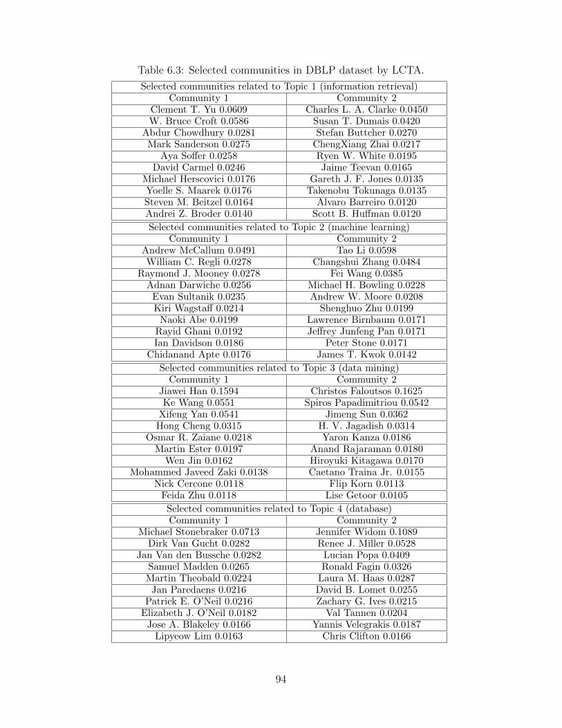
Table 6.3: Selected communities in DBLP dataset by LCTA.

Selected communities related to Topic 1 (information retrieval)Community 1 Community 2

Clement T. Yu 0.0609 Charles L. A. Clarke 0.0450W. Bruce Croft 0.0586 Susan T. Dumais 0.0420

Abdur Chowdhury 0.0281 Stefan Buttcher 0.0270Mark Sanderson 0.0275 ChengXiang Zhai 0.0217

Aya Soffer 0.0258 Ryen W. White 0.0195David Carmel 0.0246 Jaime Teevan 0.0165

Michael Herscovici 0.0176 Gareth J. F. Jones 0.0135Yoelle S. Maarek 0.0176 Takenobu Tokunaga 0.0135Steven M. Beitzel 0.0164 Alvaro Barreiro 0.0120Andrei Z. Broder 0.0140 Scott B. Huffman 0.0120

Selected communities related to Topic 2 (machine learning)Community 1 Community 2

Andrew McCallum 0.0491 Tao Li 0.0598William C. Regli 0.0278 Changshui Zhang 0.0484

Raymond J. Mooney 0.0278 Fei Wang 0.0385Adnan Darwiche 0.0256 Michael H. Bowling 0.0228

Evan Sultanik 0.0235 Andrew W. Moore 0.0208Kiri Wagstaff 0.0214 Shenghuo Zhu 0.0199

Naoki Abe 0.0199 Lawrence Birnbaum 0.0171Rayid Ghani 0.0192 Jeffrey Junfeng Pan 0.0171Ian Davidson 0.0186 Peter Stone 0.0171

Chidanand Apte 0.0176 James T. Kwok 0.0142

Selected communities related to Topic 3 (data mining)Community 1 Community 2

Jiawei Han 0.1594 Christos Faloutsos 0.1625Ke Wang 0.0551 Spiros Papadimitriou 0.0542

Xifeng Yan 0.0541 Jimeng Sun 0.0362Hong Cheng 0.0315 H. V. Jagadish 0.0314

Osmar R. Zaiane 0.0218 Yaron Kanza 0.0186Martin Ester 0.0197 Anand Rajaraman 0.0180

Wen Jin 0.0162 Hiroyuki Kitagawa 0.0170Mohammed Javeed Zaki 0.0138 Caetano Traina Jr. 0.0155

Nick Cercone 0.0118 Flip Korn 0.0113Feida Zhu 0.0118 Lise Getoor 0.0105

Selected communities related to Topic 4 (database)Community 1 Community 2

Michael Stonebraker 0.0713 Jennifer Widom 0.1089Dirk Van Gucht 0.0282 Renee J. Miller 0.0528

Jan Van den Bussche 0.0282 Lucian Popa 0.0409Samuel Madden 0.0265 Ronald Fagin 0.0326Martin Theobald 0.0224 Laura M. Haas 0.0287

Jan Paredaens 0.0216 David B. Lomet 0.0255Patrick E. O’Neil 0.0216 Zachary G. Ives 0.0215

Elizabeth J. O’Neil 0.0182 Val Tannen 0.0204Jose A. Blakeley 0.0166 Yannis Velegrakis 0.0187

Lipyeow Lim 0.0163 Chris Clifton 0.0166

94

Twitter

In Twitter dataset, we set the number of communities as 20 and the number of topics as

2. In Table 6.4, we listed two topics. Topic 1 is about Obama with its focus on health,

care, white, house, etc. Topic 2 is about social media. In Twitter, many popular users are

entrepreneurs and marketers, so its popular words in Topic 2 contain social, media, marketing

and business. Some users are technology lovers and some specialize in development and

search engine optimization, so the words like ways and tips are also popular.

Table 6.4: Topics in Twitter dataset by LCTA.

Topic 1 (Obama) Topic 2 (social media)

president 0.0064 michelle 0.0032 social 0.0153 video 0.0043

health 0.0056 administration 0.0031 media 0.0144 sites 0.0039

care 0.0052 bill 0.0031 marketing 0.0098 tools 0.0039

obama 0.0051 afghanistan 0.0031 twitter 0.0089 web 0.0038

barack 0.0046 bush 0.0029 business 0.0077 online 0.0038

speech 0.0044 nobel 0.0029 blog 0.0056 brand 0.0037

reform 0.0038 peace 0.0027 facebook 0.0049 company 0.0035

white 0.0038 calls 0.0026 ways 0.0046 roi 0.0032

house 0.0037 poll 0.0026 post 0.0046 expert 0.0030

plan 0.0035 iran 0.0026 tips 0.0045 guide 0.0030

We show several selected communities and their user distributions in Table 6.5. In the

communities related to topic Obama, Community 1 is about news media. For example,

NPR Politics is political coverage and conversation from NPR News. NewsHour is one of

the most trusted news programs on TV. David Shuster is a journalist for NBC News and

MSNBC. Karl Rove is the former deputy chief of staff to President George W. Bush and is

the author of Courage and Consequence. Community 2 is a community about conservative

politics. For example, MichaelPatrick Leahy is the author of Rules for Conservative Radicals.

ChadTEverson is a conservative activist. Nansen Malin is a student who does conservative

politics. Most of the users in the communities related to social media are entrepreneurs,

strategists, authors, speakers, business coaches, etc. For example, Zee M Kane is the editor-

95

in-chief of The Next Web. Robert Clay is an entrepreneur and business mentor to aspiring

market leaders. Jonathan Nafarrete is a social media strategist.

Table 6.5: Selected communities in Twitter dataset by LCTA.

Selected communities related to Topic 1 (Obama)

Community 1 Community 2

NPR Politics 0.0249 Tabitha Hale 0.0093

Paula Poundstone 0.0207 MichaelPatrick Leahy 0.0075

Los Angeles Times 0.0166 Infidels Are Cool 0.0068

NPR News 0.0142 It’s Only Words 0.0064

Redeye Chicago 0.0135 Justin Hart 0.0061

Jim Long 0.0134 michaelemlong 0.0061

NewsHour 0.0107 ChadTEverson 0.0058

Steve Garfield 0.0103 Nansen Malin 0.0057

David Shuster 0.0101 Markham Robinson 0.0055

Karl Rove 0.0092 Andrew Windham 0.0055

Selected communities related to Topic 2 (social media)

Community 1 Community 2

Social Media Insider 0.0062 Robert Clay 0.0092

Jeff Flowers 0.0061 Jonathan Nafarrete 0.0091

Wolfgang Jaegel 0.0059 Andrew Windham 0.0091

Zee M Kane 0.0059 Arleen Boyd 0.0083

Mark Fulton 0.0056 Bobby Bloggeries 0.0077

Social Media News 0.0054 Montaignejns 0.0076

Nick Donnelly 0.0052 Glen Gilmore 0.0074

Brian Tercero 0.0048 Larry Brauner 0.0071

Alex Blom 0.0045 Guy Kawasaki 0.0071

Monik Pamecha 0.0044 Jay Oatway 0.0070

6.4.3 Comparison with Community Discovery Methods

Our LCTA (Latent Community Topic Analysis) model is closely related to community dis-

covery. LCTA can handle community discovery and topic modeling simultaneously. Specif-

ically, in LCTA topics are generated from different communities. In this way we guarantee

topical coherence in the community level. It is interesting to compare the performance of

our model with community discovery methods.

96

We compare the following methods in this section.

• NormCut [91]: Normalized cut algorithm on a link graph.

• SSNLDA [113]: An LDA-based hierarchical Bayesian algorithm on a link graph where

communities are modeled as latent variables and defined as distributions over user

space.

• LCTA: Our Latent Community Topic Analysis model that integrates community dis-

covery with topic modeling.

To compare the discovered topics from LCTA with the ones based on NormCut and

SSNLDA, we first use NormCut and SSNLDA to cluster the link graph into 20 communities

in both datasets and pool the text of the users in the same community together. We consider

the text in each community as a document and run topic modeling method PLSA [44] on the

collection. We set the number of topics as 4. NormCut+PLSA and SSNLDA+PLSA can be

considered as the approaches to discover topics based on clustered communities. The topics

discovered by NormCut+PLSA and SSNLDA+PLSA in DBLP dataset are listed in Table 6.6

and Table 6.7. We can see the topics discovered by NormCut+PLSA and SSNLDA+PLSA

are not meaningful and the result by LCTA in Table 6.2 is much better. The topics discovered

by NormCut+PLSA and SSNLDA+PLSA in Twitter dataset are listed in Table 6.8. We

can see that compared with the result by LCTA in Table 6.4, the topics discovered by these

two approaches are not pure enough. In Table 6.8, the topic related to Obama contains

the terms like social media, while the topic related to social media also contains the term

obama. Therefore we can see that our LCTA model considering community discovery and

topic modeling in a unified framework performs better than those approaches processing

community discovery and topic modeling separately.

Besides the qualitative evaluation, we also quantitatively evaluate the topical coher-

ence. In DBLP dataset, each user is categorized into one domain of data mining, databases,

97

Table 6.6: Topics in DBLP dataset by NormCut+PLSA.

Topic 1 Topic 2 Topic 3 Topic 4

data 0.0241 data 0.0326 learning 0.0215 retrieval 0.0237mining 0.0171 database 0.0142 web 0.0163 information 0.0167

clustering 0.0109 query 0.0139 search 0.0108 data 0.0141system 0.0095 queries 0.0118 mining 0.0102 learning 0.0114learning 0.0091 databases 0.0107 data 0.0100 search 0.0108

databases 0.0089 xml 0.0105 query 0.0069 system 0.0106efficient 0.0087 efficient 0.0097 information 0.0068 web 0.0098

information 0.0086 mining 0.0086 classification 0.0066 query 0.0088database 0.0085 web 0.0085 model 0.0065 text 0.0085approach 0.0076 system 0.0082 approach 0.0063 document 0.0073

Table 6.7: Topics in DBLP dataset by SSNLDA+PLSA.

Topic 1 Topic 2 Topic 3 Topic 4

data 0.0325 data 0.0248 data 0.0286 data 0.0243database 0.0148 learning 0.0138 learning 0.0123 mining 0.0199

query 0.0132 retrieval 0.0124 mining 0.0114 web 0.0154system 0.0111 information 0.0111 query 0.0109 search 0.0130learning 0.0099 query 0.0093 information 0.0102 learning 0.0123

databases 0.0098 mining 0.0093 system 0.0100 information 0.0112queries 0.0096 database 0.0093 database 0.0096 retrieval 0.0112systems 0.0094 system 0.0092 databases 0.0093 query 0.0103efficient 0.0089 search 0.0079 web 0.0085 databases 0.0102

clustering 0.0088 efficient 0.0078 retrieval 0.0082 efficient 0.0101

Table 6.8: Topics in Twitter dataset by NormCut+PLSA and SSNLDA+PLSA.

NormCut+PLSA SSNLDA+PLSA

Topic 1 Topic 2 Topic 1 Topic 2obama 0.0103 media 0.0099 obama 0.0102 media 0.0145

president 0.0065 social 0.0096 president 0.0067 social 0.0141health 0.0047 marketing 0.0061 health 0.0054 obama 0.0103care 0.0047 twitter 0.0058 care 0.0050 twitter 0.0081

media 0.0041 business 0.0050 media 0.0048 marketing 0.0075speech 0.0040 blog 0.0041 speech 0.0047 business 0.0067social 0.0038 top 0.0039 social 0.0039 video 0.0059white 0.0036 obama 0.0037 white 0.0038 top 0.0056barack 0.0034 great 0.0036 reform 0.0037 blog 0.0054house 0.0034 video 0.0036 house 0.0036 great 0.0051

98

machine learning and information retrieval according to the labeling in [32]. Therefore, ac-

curacy and normalized mutual information (NMI) [10] can be used to measure the clustering

performance and topical coherence in DBLP dataset.

Accuracy Given user u, its label su in the dataset and the assigned label ru obtained

from the above methods, accuracy is defined as follows.

Accuracy =

∑u∈U δ(su,map(ru))

|U |

where |U | is the number of all the users and δ(x, y) is the delta function that is one if x = y

and is zero otherwise, and map(ru) is the permutation mapping function that maps the label

ru of user u to the corresponding label in the dataset. The best mapping between the labels

can be found by Kuhn-Munkres algorithm [51].

Normalized Mutual Information We denote C as the user labels obtained from the dataset

and C ′ as the ones obtained from the above methods. The mutual information metric

MI(C,C ′) is defined as follows.

MI(C,C ′) =∑

c∈C,c′∈C′p(c, c′) log

p(c, c′)

p(c)p(c′)

where p(c) is the probability that a user arbitrarily selected from the dataset has label c,

and p(c, c′) is the joint probability that the arbitrarily selected document has label c and is

assigned with label c′. The normalized mutual information NMI is defined as follows.

NMI(C,C ′) =MI(C,C ′)

max(H(C), H(C ′))(6.11)

where H(C) is the entropy of C. Specifically, NMI = 1 if C and C ′ are identical, and NMI

= 0 if C and C ′ are independent.

We show the result of accuracy and normalized mutual information in DBLP dataset in

Table 6.9. From the table, we can see that LCTA performs the best among all the methods.

99

Table 6.9: Accuracy and NMI by NormCut, SSNLDA and LCTA.

NAccuracy(%) NMI(%)

NormCut SSNLDA LCTA NormCut SSNLDA LCTA5 36.78 29.46 72.19 2.02 1.41 43.7910 41.43 23.56 54.81 8.34 1.72 31.7715 36.99 21.12 37.74 10.01 2.29 25.6620 33.45 18.81 35.10 9.01 1.71 23.46

The labels of the users in DBLP dataset mainly consider the coherence of topics. Since

NormCut and SSNLDA do not consider the text information, both of them perform poor in

the dataset. When the number of communities is large such as 15 and 20, NormCut performs

relatively well in accuracy measure. The reason is that in the result of NormCut there is

a small number of very large communities while in the result of other methods the clusters

are of similar sizes. There are only four types of labels in DBLP dataset. If the result is

dominant by one big cluster, the cluster can be mapped to one of the four labels, so the

result will have a relatively large accuracy value. Therefore, accuracy may not be a good

measure to compare the performance especially when the number of communities is large,

so we use normalized mutual information as additional evaluation measure. In normalized

mutual information both NormCut and SSNLDA perform poorly. Therefore we can see that

our LCTA model performs better than those approaches processing community discovery

and topic modeling separately.

6.4.4 Comparison with Topic Modeling Methods

In this section we compare our LCTA (Latent Community Topic Analysis) model with other

topic modeling methods.

We compare the following methods in this section.

• PLSA [44]: Probabilistic latent semantic analysis.

• NetPLSA [68]: PLSA regularized with a harmonic regularizer based on a link graph

100

structure.

• LinkLDA [26]: A generative model of both text and links where words and links are

generated according to the same latent topic space.

• LCTA: Our Latent Community Topic Analysis model that integrates community dis-

covery with topic modeling.

The latent topics discovered by PLSA, NetPLSA and LinkLDA can also be used to

calculate the clusters of users. Similarly accuracy and normalized mutual information (NMI)

can be used to measure the clustering performance and topical coherence in DBLP dataset

for comparing different methods.

Table 6.10: Accuracy and NMI by PLSA, NetPLSA, LinkLDA and LCTA.

NAccuracy(%) NMI(%)

PLSA NetPLSA LinkLDA LCTA PLSA NetPLSA LinkLDA LCTA5 67.55 68.09 69.33 72.19 41.29 42.49 40.50 43.7910 44.54 45.96 44.05 54.81 28.71 29.05 26.86 31.7715 33.39 34.23 32.48 37.74 22.36 23.09 21.72 25.6620 25.89 26.42 26.67 35.10 20.06 21.24 18.73 23.46

The comparison result of both accuracy and normalized mutual information is listed in

Table 6.10. From the table we can see that our LCTA model performs the best among all the

methods. Compared with PLSA, NetPLSA considers the link graph structure to regularize

the topic modeling process, so it has a better performance than PLSA. Our LCTA model

separates the concepts of topic and community and it performs better than LinkLDA in

which both words and links are generated according to the same latent topic space.

Beside evaluating the topical coherence, we also compare the link structure coherence

for different topic modeling methods. From the clusters of users by PLSA, NetPLSA and

LinkLDA, we can calculate the normalized cut measure based on the partition of the graphs.

Normalized Cut Normalized cut (Ncut) is defined as Ncut =∑N

i=1cut(Ci,U−Ci)assoc(Ci,U)

, where

cut(A,B) =∑

u∈A,v∈B n(u, v), assoc(A,U) =∑

s∈A,t∈U n(s, t) and Ci is the i-th community.

101

cut(A,B) is the total weight of the edges that have been removed by disconnecting two parts

A and B. assoc(A,U) is the total connection from nodes in A to all the nodes in the graph.

Table 6.11: Normalized cut in DBLP dataset by PLSA, NetPLSA, LinkLDA and LCTA.

N PLSA NetPLSA LinkLDA LCTA

5 2.36 2.15 2.35 1.8910 6.82 6.70 6.00 5.6015 12.52 11.77 11.12 10.5320 16.70 16.29 15.84 15.69

Table 6.12: Normalized cut in Twitter dataset by PLSA, NetPLSA, LinkLDA and LCTA.

N PLSA NetPLSA LinkLDA LCTA

5 7.85 6.87 7.10 6.1110 17.80 16.25 16.78 16.2415 27.80 26.29 26.76 25.9120 37.72 35.84 36.23 35.47

We list the result of DBLP dataset in Table 6.11 and the one of Twitter dataset in Ta-

ble 6.12. In both datasets, compared with other methods, LCTA performs better, which

means that LCTA considers the link information relatively well and can discover more co-

herent communities.

6.4.5 Parameter Setting

In this section, we study the effect of parameter changes on the result. We have to set two

parameters in our model, i.e., the number of communities and the number of topics.

To study the effect of the number of communities, we build a subset of DBLP dataset

including all the co-authors of Hector Garcia-Molina, Rakesh Agrawal, Christos Faloutsos

and Jiawei Han, which results in a graph of 494 users. We set the number of communities

as 4 and 20 separately and compare the discovered communities. In Table 6.13, we can see

that if we set the number of communities as 4 there are four communities related to these

four researchers. We increase the number of communities from 4 to 20 and show the selected

102

communities related to Christos Faloutsos and Jiawei Han in Table 6.14. Community 1 of

Christos Faloutsos is about his community at Carnegie Mellon University and Community

2 is about his community along with Yahoo Research and Cornell University. Community

1 of Jiawei Han is about his community at University of Illinois at Urbana and Champaign

including his students Xifeng Yan, Dong Xin, etc. Community 2 is another collaboration

community of Jiawei Han. From this example, we can see that if we set the number of com-

munities to a small value, we can have communities of coarse granularity. If we increase the

number of communities, coarse communities will break down into the ones of fine granularity.

Table 6.13: Communities when the number of communities is 4.

Community 1 (Hector Garcia-Molina) Community 2 (Rakesh Agrawal)

Hector Garcia-Molina 0.1395 Rakesh Agrawal 0.1200Jennifer Widom 0.0455 Ramakrishnan Srikant 0.0369

Jeffrey D. Ullman 0.0425 Surajit Chaudhuri 0.0340Rajeev Motwani 0.0325 Michael J. Carey 0.0313Sharad Mehrotra 0.0213 Raghu Ramakrishnan 0.0308

Abraham Silberschatz 0.0190 Hamid Pirahesh 0.0282Yannis Papakonstantinou 0.0186 Jeffrey F. Naughton 0.0277

Janet L. Wiener 0.0179 David J. DeWitt 0.0262Serge Abiteboul 0.0163 Jerry Kiernan 0.0190Wilburt Labio 0.0159 Umeshwar Dayal 0.0175

Community 3 (Christos Faloutsos) Community 4 (Jiawei Han)

Christos Faloutsos 0.1513 Jiawei Han 0.1719Andrew Tomkins 0.0300 Jian Pei 0.0482

Ravi Kumar 0.0298 Wei Wang 0.0440Spiros Papadimitriou 0.0282 Xifeng Yan 0.0302

Jure Leskovec 0.0243 Jeffrey Xu Yu 0.0239H. V. Jagadish 0.0236 Ke Wang 0.0235

Dimitris Papadias 0.0195 Hongjun Lu 0.0222Jimeng Sun 0.0195 Hong Cheng 0.0214

Raymond T. Ng 0.0188 Dong Xin 0.0209Agma J. M. Traina 0.0183 Haixun Wang 0.0201

To study the effect of the number of topics, we vary the number of topics and compare

the the results. If we set the number of topics as 4, from Table 6.2, we can get the four

topics including information retrieval, machine learning, data mining and database. If we

103

Table 6.14: Selected communities when the number of communities is 20.

Selected communities related to Christos Faloutsos

Community 1 Community 2Christos Faloutsos 0.2322 Ravi Kumar 0.1451

Spiros Papadimitriou 0.0521 Andrew Tomkins 0.1451Jimeng Sun 0.0426 Christos Faloutsos 0.1043

Dimitris Papadias 0.0412 Jure Leskovec 0.0915Yufei Tao 0.0400 Prabhakar Raghavan 0.0444

Agma J. M. Traina 0.0386 Carlos Guestrin 0.0349Caetano Traina Jr. 0.0297 Andreas Krause 0.0349

Hanghang Tong 0.0242 Marko Grobelnik 0.0296Nick Roussopoulos 0.0220 Jon M. Kleinberg 0.0296

Jia-Yu Pan 0.0219 Sridhar Rajagopalan 0.027

Selected communities related to Jiawei Han

Community 1 Community 2Jiawei Han 0.2576 Jiawei Han 0.1418Xifeng Yan 0.0950 Wei Wang 0.1060Dong Xin 0.0654 Anthony K. H. Tung 0.0919Xiaolei Li 0.0601 Wen Jin 0.0792

Hong Cheng 0.0594 Haixun Wang 0.0767Hector Gonzalez 0.0271 Hongjun Lu 0.0696

Xiaoxin Yin 0.0237 Martin Ester 0.0550Tianyi Wu 0.0224 Jian Pei 0.0371Chen Chen 0.0195 Nick Koudas 0.0326Feida Zhu 0.0180 Jiong Yang 0.0301

increase the number of topics from 4 to 20, we can have the topics of fine granularity. In

Table 6.15, we list several topics related to database and machine learning when the number

of topics is 20. The first topic related to database is about relational database and query

optimization, and the second is about spatial temporal database. The first topic related to

machine learning is about bayesian networks and kernel methods, and the second is learning

in computer vision.

104

Table 6.15: Selected topics in DBLP dataset when the number of topics is 20.

Selected topics related to database Selected topics related to machine learning

Topic 1 Topic 2 Topic 1 Topic 2query 0.0344 queries 0.0385 learning 0.0478 image 0.0285

database 0.0339 temporal 0.0383 bayesian 0.0226 recognition 0.0268relational 0.0294 spatial 0.0316 networks 0.0189 visual 0.0177queries 0.0284 efficient 0.0274 supervised 0.0185 learning 0.0160

databases 0.0229 processing 0.0197 analysis 0.0181 motion 0.0144sql 0.0190 objects 0.0163 classification 0.0155 shape 0.0129

optimization 0.0185 spatio 0.0153 kernel 0.0124 3d 0.0117object 0.0150 moving 0.0146 models 0.0121 vision 0.0111

relations 0.0122 indexing 0.0122 fast 0.0103 interactive 0.0107views 0.0117 multidimensional 0.0119 markov 0.0099 fuzzy 0.0104

6.5 Conclusion and Future Work

With the development of social media a lot of user-generated content is available with user

networks. The user graphs extended with text information on the nodes form text-associated

graphs. We study the problem of latent community topic analysis in text-associated graphs

and propose a model called LCTA to incorporate community discovery into topic modeling.

We handle topic modeling and community discovery in the same framework to guarantee

the topical coherence in the communities. We perform extensive experiments on two real

datasets and show that our model outperforms other methods.

Our work opens up several interesting future directions. First, the communities in our

LCTA model are of the same level but the communities in real world may have hierarchical

structure. It is interesting to extend our framework to hierarchical community discovery

scenarios by bottom-up or top-down strategy. Second, the user-generated content in social

media sites includes not only text data but also other rich information such as pictures,

time, and spatial information. It is interesting to integrate those heterogeneous information

together in the framework.

105

Chapter 7

Trajectory Pattern Ranking

7.1 Introduction

Social media is becoming increasingly popular with the development of Web 2.0. Social media

websites such as Flickr, Facebook, and YouTube host overwhelming amounts of photos and

videos. In such a media sharing community, image or video files are contributed, tagged,

and commented by users all over the world. Extra information can be incorporated within

social media, such as geographical information captured by GPS devices. Studying such

social media attracts both academic and industrial interests, and it has been a hot research

area in recent years [84, 22, 82, 81, 11, 18, 64].

Our goal is to explore the common wisdom in photo sharing community. We study

millions of personal photos in Flickr, which are associated with user tags and geographical

information. The geographical information is captured by low-cost GPS chips in cell phones

and cameras, and often saved in the header of image files. Going beyond the recent work on

using Flickr photos to match tourist interests in terms of locations [82, 81, 11], we focus on

trajectory patterns. We would like to discover trajectory patterns interesting to two kinds

of users. First, some users are interested in the most important trajectory patterns. When

they visit a new city, they would like to follow those trajectories that concentrate on popular

locations that lots of people are interested in. Second, some users are interested in exploring

a new place in diverse ways. They are not only interested in the most important trajectories,

but also eager to explore other routes to cover the entire area. Instead of focusing on how

to mine frequent trajectory patterns, we put more effort into ranking the mined trajectory

106

patterns and diversifying the ranking results. Trajectory pattern ranking helps the first

kind of users who are interested in top important trajectories, while diversification helps

the second kind of users that are willing to explore the diverse routes. There are some

studies on trip planning using Flickr. In [18, 17], Choudhury et al. formulated trip planning

as directed orienteering problem. In [64], Lu et al. used dynamic programming for trip

planning. In [53], Kurashima et al. recommended tourist routes by combining topic models

and Markov model. However, diversified trajectory pattern ranking has not been investigated

in geo-tagged social media before. After aggregating the trajectories by pattern mining, we

investigate the problem of ranking trajectory patterns and diversifying the ranking results.

Trajectory mining has been investigated in many datasets including animal movement [55],

hurricane tracking [55], urban traffic [36, 35], human travel history [118, 117], etc.. Gian-

notti et al. developed a spatial-temporal pattern mining paradigm that discovers trajectory

patterns [36]. We mine trajectory patterns from geo-tagged social media, where trajectory

patterns are represented by a sequence of locations according to temporal order. Usually the

pattern mining result is a set of mined patterns with their frequencies. However, this kind

of representation has several disadvantages. First, there are too many trajectory patterns

in the result. It is difficult for users to go through all the patterns in the list to discover the

interesting ones. As a result, the interesting trajectory patterns are buried in the massive

result set. Second, if we only return the top frequent trajectory patterns as results, the re-

sults may not be interesting to all users. One reason is that top frequent trajectory patterns

are usually short and not informative. Third, many trajectory patterns are similar, so re-

dundant information exists in the results. Many frequent trajectory patterns share common

sub-patterns, so it is not interesting to output all of them. To overcome the above problems,

we propose an algorithm to rank trajectory patterns by considering the relationships among

users, locations and trajectories, and introduce an exemplar-based algorithm to diversify

trajectory pattern ranking results.

107

7.2 Problem Definition

In geo-tagged social media sites such as Flickr, a large collection of photos is uploaded by

users. Each photo is taken by a user at specific location and time. The location is annotated

by GPS coordinate (x, y), where x refers to longitude and y refers to latitude. Here are a

few definitions that we used.

Definition 12. Location is a popular region that users visit.

Definition 13. Trajectory is a sequence of locations visited by a user according to tem-

poral order during the same day1.

Definition 14. Trajectory pattern is a sequence of locations whose frequency is no smaller

than minimum support. The sequence frequency is defined as the number of users visiting

the locations according to the order in the sequence. We only discuss the trajectory patterns

without duration constraints.

The problem of diversified trajectory pattern ranking in geo-tagged social media is formu-

lated as given a collection of geo-tagged photos along with users, locations and timestamps,

how to rank the mined trajectory patterns with diversification into consideration.

Our framework consists of three main components: (1) extracting trajectory patterns

from the photo collection, (2) ranking the trajectory patterns by estimating their importance

according to user, location and trajectory pattern relations, and (3) diversifying the ranking

result to identify the representative trajectory patterns from all the candidates. We will

explain these components one by one. Though geo-tagged social media is taken as an

example, our technique can be applied to other trajectory pattern ranking scenarios.

1We can extend the trajectory to span multiple days. We only discuss the scenario within the same daywithout loss of generality.

108

7.3 Trajectory Pattern Mining Preliminary

In this section, we introduce how to mine frequent trajectory patterns in geo-tagged photo

collections such as those in Flickr. Since the GPS coordinates of photos are at a very fine

granularity, we need to detect locations before extracting trajectory patterns. This process

is similar to discovering ROI (region of interest) in [36]. With the detected locations, we can

generate the trajectories for each user according to his visiting order of the locations during

the same day. Then we can mine the frequent trajectory patterns using sequential pattern

mining. If a trajectory pattern repeats frequently, we consider it as a frequent trajectory

pattern.

7.3.1 Location Detection

We cluster the photo GPS coordinates to detect the locations. The location clustering process

should satisfy the following criteria: (1) The close-by points should be grouped together, (2)

clustering should accommodate arbitrary shapes, and (3) the clustering parameters should

be easy to set according to the application scenario. Considering all the aspects, we use the

mean-shift algorithm [16, 21] to extract locations. Mean-shift is an iterative procedure that

shifts each data point to the average of data points in its neighborhood.

m(x) =

∑s∈SK(s− x)s

K(s− x)s

where S is the set of all the data points. The difference m(x)−x is the mean shift. x→ m(x)

is performed for all s ∈ S simultaneously to move the data point to its sample mean and

this process repeats until convergence. In our case, the location of a photo is considered as

a data point. If one user takes multiple photos at the same place, it is only counted as one

point. Here we use a flat kernel function and set the bandwidth λ as 0.001. 0.001 in GPS

coordinate is approximately 100m. We assume that a reasonable extent for typical locations

109

is around 100 meters in diameter, so we use 0.001 as the bandwidth for mean-shift clustering.

We use a flat kernel as follows.

K(x) =

1 if ‖x‖ ≤ λ

0 if ‖x‖ > λ.

7.3.2 Location Description

After getting the locations in Section 7.3.1, we need to generate the descriptions for the

locations. For each photo in Flickr, besides the GPS location, we also have associated tags

that are contributed by users. Here we use a generative mixture model to extract useful tags

for each location.

Given location L, we assume that the tags of the photos in location L are generated from

a background model B and a corresponding location model θL. The background model B

is represented by a tag distribution p(t|B) where∑

t p(t|B) = 1, while the location model

θL is represented by another tag distribution p(t|θL) where∑

t p(t|θL) = 1. Given the photo

collection CL of location L, we want to find p∗(t|θL) that maximizes the following likelihood.

log p(CL|θ) =∑t

c(t, L) log[(1− λ)p(t|θL) + λp(t|B)]

where t is tag and c(t, L) is the count of the users that contribute tag t in location L. Here

we use the count of the users instead of the count of the photos for the reason that one user

may take many photos at the same location. Therefore, the count of the users is better to

represent the popularity of the tag for the specific location. λ is the tradeoff between the

background model B and the location model θL. We set λ as 0.8 empirically here. p(t|B)

can be obtained by considering the tags in all the locations, i.e., p(t|B) = c(t)∑t c(t)

where c(t)

is the count of the users that contribute tag t in the whole collection, and p∗(t|θL) that

maximizes the above likelihood can be estimated by EM algorithm. We introduce hidden

110

variable zt, where zt = 1 means that tag t is from background B and zt = 0 means that tag

t is from location model θL.

In E-step,

p(zt = 1|t) =λp(t|C)

λp(t|C) + (1− λ)p(t|θL)

In M-step,

p(t|θL) =c(t)(1− p(zt = 1|t))∑t c(t)(1− p(zt = 1|t))

We calculate p∗(t|θL) for location L and use the top tags to annotate location L. The

descriptions for top locations in London is listed in Table 7.1. From Table 7.1, we can find

that the tags such as uk and london are not included in the top tags for the location with

the above smoothing.

As an example, we crawled 27974 photos in London area from Flickr and clustered 883

locations. The top locations associated with their tag descriptions are listed in Table 7.1.

Table 7.1: Top locations in London and their descriptions.

londoneye(528), trafalgarsquare(456), britishmuseum(230), bigben(205),

waterloobridge(198), towerbridge(185), piccadillycircus(182), royalfestivalhall(175),

coventgarden(169), centrepoint(169), parliamentsquare(150), cityhall(141),

oxfordcircus(138), lloyds(121), buckinghampalace(107), naturalhistorymuseum(97),

canarywharf(94), bricklane(91), toweroflondon(91), brighton(90), embankment(88),

soho(80), stpancras(77), stpaulscathedral(77), leicestersquare(76),

gherkin(75), stjamespark(68), barbican(67), victoriaandalbertmuseum(64)

*The number in the parentheses is the number of users visiting the place.

7.3.3 Sequential Pattern Mining

After the location clustering step, we generate the trajectories according to the visiting order

of the locations. We use the PrefixSpan algorithm [80] to extract the frequent sequential

patterns and treat them as trajectory patterns. Given a set of sequences, sequential pat-

111

tern mining algorithm will find all the sequential patterns whose frequencies are no smaller

than the minimum support. The frequency of a pattern is defined as the number of se-

quences subsuming the pattern. We set the minimum support threshold as 2 to collect as

many trajectory patterns as possible for ranking. Here we show a sequential pattern mining

example.

Table 7.2: An example of sequential pattern mining.

ID Travel sequence

1 londoneye → bigben → trafalgarsquare2 londoneye → bigben → downingstreet → trafalgarsquare3 londoneye → bigben → westminster4 londoneye → tatemodern → towerbridge5 londoneye → bigben → tatemodern

Example 7. Given 5 sequences in Table 7.2 and a minimum support of 2, we find the

following three patterns: londoneye → bigben has a frequency of 4, since it is contained in

sequences 1, 2, 3 and 5. londoneye → bigben → trafalgarsquare has a frequency of 2, since

it is contained in sequences 1 and 2. londoneye → tatemodern has a frequency of 2, since it

is contained in both sequences 4 and 5.

After clustering 883 locations in London in the previous stage, we generate 4712 trajec-

tories. We mine 1202 trajectory patterns from these trajectories and list the top frequent

trajectory patterns in London in Table 7.3, where the location descriptions are generated in

Section 7.3.2. From Table 7.3, we find that the most frequent trajectory patterns contain

important locations but reveal limited information. These frequent patterns are short and

not informative, so we need a better ranking mechanism to organize the mined patterns.

7.4 Trajectory Pattern Ranking

In this section, we discuss how to rank the mined trajectory pattern without considering

diversification. First, we discuss the needs of trajectory pattern ranking and introduce the

112

Table 7.3: Top frequent trajectory patterns in London.

Rank Trajectory pattern Frequency

1 londoneye → bigben 212 bigben → londoneye 193 londoneye → tatemodern 184 londoneye → royalfestivalhall 155 londoneye → trafalgarsquare 146 londoneye → waterloobridge 127 towerbridge → cityhall 128 royalfestivalhall → londoneye 119 tatemodern → londoneye 1110 bigben → parliamentsquare 10

general idea about our ranking strategy. Second, we describe our ranking algorithm in detail.

Third, we analyze the complexity of the algorithm and give the convergence proof.

7.4.1 General Idea

In the previous stage, we extract all the frequent sequential patterns as trajectory patterns.

In this way, the common movement behaviors are extracted from the data collection. How-

ever, there are too many trajectory patterns and it is difficult for users to browse all the

candidates. Therefore, a ranking mechanism is needed for these trajectory patterns. We

can simply rank all these trajectory patterns by their frequencies as in Table 7.3, where

frequency refers to the number of users visiting the sequence. As one can see in Table 7.3,

all the top ten trajectory patterns ranked by frequency are of length 2. Although the top

frequent trajectory patterns cover the important locations such as londoneye, bigben and

tatemodern, they are not informative for the reason that people are more interested in the

sequential order of locations. In order to derive better importance measure of a trajectory

pattern, we need to consider more aspects about geo-tagged social media.

In geo-tagged social media, relationships among users, locations and trajectories are

embedded in the dataset as illustrated in Figure 7.1. Specifically, a trajectory is a sequence

of locations visited by users, and its importance should be influenced both by users and

113

Figure 7.1: Relationship among user, location and trajectory in geo-tagged social media.

locations. Here we propose a ranking algorithm to explore such relations. The assumptions

that we make here are listed as follows.

1. A trajectory pattern is important if many important users take it and it contains

important locations,

2. a user is important if the user takes photos at important locations and visits the

important trajectory patterns, and

3. a location is important if it occurs in one or more important trajectory patterns and

many important users take photos at the location.

7.4.2 Ranking Algorithm

We denote the importance scores of users, locations and trajectory patterns as PU , PL and

PT . PU , PL and PT are all vectors. Each element in the vector is the importance score of

the corresponding unit. The relationship between PU , PL and PT are as follows according

to the above assumptions.

PL = MLT · PT PU = MUL · PL

114

PT = MTU · PU PU = MTTU · PT

PL = MTUL · PU PT = MT

LT · PL

MTU is the trajectory-user matrix, and its entry indicates the ownership of a trajectory

for a user. MUL is the user-location matrix indicating whether a user takes a photo at a

location. MLT is the location-trajectory matrix indicating whether a location is contained

in a trajectory or not.

We summarize the trajectory pattern ranking algorithm in Algorithm 1. The importance

scores of users, locations and trajectories mutually enhance each other according to the

assumptions until convergence.

Algorithm 1 Trajectory pattern ranking

Input: MTU , MUL, MLT

Output: A ranked list of trajectory patterns

1. Initialize P(0)T

2. Iterate

PL = MLT · P (t)T PU = MUL · PL

PT = MTU · PU PU = MTTU · PT

PL = MTUL · PU P

(t+1)T = MT

LT · PL

P(t+1)T = P

(t+1)T /‖P (t+1)

T ‖1

until convergence.

3. Output the ranked list of trajectory patterns in the decreasing order of P ∗T , i.e., the

converged PT .

115

To illustrate the updating procedure, we use a toy example with 3 users and 4 trajectory

patterns to characterize how PL, PU , and PT evolve in each iteration in Table 7.4. Note that

the importance scores are normalized for better understanding.

Table 7.4: A toy example of trajectory pattern ranking.

Trajectory patterns with user and location information.

Trajectory index User index Location sequence

T1 U1 L1, L2, L3T2 U1 L3, L4T3 U2 L1, L3T4 U3 L3, L4

Importance scores updating process.

Iteration 1 2 3 4

Trajectories

T1 0.2500 0.3077 0.3090 0.3088T2 0.2500 0.2308 0.2300 0.2299T3 0.2500 0.2308 0.2310 0.2313T4 0.2500 0.2308 0.2300 0.2299

Users

U1 0.3333 0.6061 0.6060 0.6062U2 0.3333 0.2020 0.2020 0.2022U3 0.3333 0.1919 0.1920 0.1917

Locations

L1 0.2500 0.2516 0.2520 0.2516L2 0.2500 0.1887 0.1890 0.1887L3 0.2500 0.3113 0.3110 0.3113L4 0.2500 0.2484 0.2480 0.2484

We list the trajectory pattern ranking result in London in Table 7.5. Although the tra-

jectory pattern frequencies are low, they are visited by important users and cover important

locations. Compared with the top frequent trajectory patterns in Table 7.3, the trajectory

patterns ranked by our model are more informative.

In Algorithm 1, not only can we estimate the importance of trajectories, but we can

also get the location importance according to PL. The top locations according to PL from

London are listed in Table 7.6. The user count of the locations stands for the number of

the users visiting the location. We find that the location importance is not determined by

user count alone. For example, horseguards is important for trajectory pattern ranking even

116

Table 7.5: Top ranked trajectory patterns in London.

Rank Trajectory pattern PT Freq.

1 londoneye → bigben → downingstreet → horseguards → trafalgarsquare 0.0037 2

2 londoneye → bigben → tatemodern 0.0029 2

3 tatemodern → bigben → londoneye 0.0029 3

4 londoneye → bigben → parliamentsquare → westminster 0.0028 2

5 westminster → bigben → downingstreet → horseguards → trafalgarsquare 0.0028 2

6 royalfestivalhall → londoneye → bigben 0.0027 2

7 londoneye → royalfestivalhall → tatemodern 0.0027 3

8 tatemodern → londoneye → royalfestivalhall 0.0027 2

9 londoneye → tatemodern → towerbridge 0.0027 2

10 londoneye → towerbridge → tatemodern 0.0027 2

though it only has a user count of 25. The reason is that horseguards is on the popular

trajectory from bigben to trafalgarsquare.

7.4.3 Discussion

In Algorithm 1, we consider the importance vector of trajectory patterns P ∗T as the eigen

vector for MT ·M for the largest eigen value, where M = MTU ·MUL ·MLT . We find that

Algorithm 1 is a normalized power iteration method to detect the eigen vector of MT ·M

for the largest eigen value if P(0)T is not orthogonal to it. Therefore, the convergence of the

algorithm is guaranteed according to convergence property of normalized power iteration

method [43].

In Algorithm 1, each iteration requires the multiplication of MT ·M and PL, so it need

O(|E|), where |E| is the number of nonzero elements in MT ·M . In total, the time complexity

of the algorithm is O(k|E|), where k is the iteration number.

7.5 Trajectory Pattern Diversification

In this section, we discuss the diversification of trajectory pattern ranking results. First, we

discuss why we need to diversify the ranking results. Second, we propose an exemplar-based

117

Table 7.6: Top ranked locations in London with normalized PL scores.

Location PL # User Location PL # User

londoneye 0.0157 528 southwark 0.0062 57

trafalgarsquare 0.0125 456 stpaulscathedral 0.0058 77

bigben 0.0121 205 downingstreet 0.0053 52

tatemodern 0.0119 491 horseguards 0.0051 25

royalfestivalhall 0.0093 175 londonbridge 0.0049 37

towerbridge 0.0089 185 embankment 0.0047 23

cityhall 0.0077 141 harrods 0.0047 39

waterloobridge 0.0076 198 toweroflondon 0.0046 91

parliamentsquare 0.0075 150 naturalhistorymuseum 0.0046 97

piccadillycircus 0.0074 182 monument 0.0046 59

britishmuseum 0.0074 230 victoriaandalbertmuseum 0.0045 64

gherkin 0.0073 75 bank 0.0044 63

lloyds 0.0070 121 royalacademy 0.0040 34

coventgarden 0.0070 169 oxfordstreet 0.0040 51

buckinghampalace 0.0064 107 bloomsbury 0.0038 27

algorithm to discover representative trajectory patterns. Third, we analyze the algorithm

complexity and give some discussion.

7.5.1 General Idea

Although our algorithm in Section 7.4 works well in ranking trajectory patterns, the results

may not satisfy the needs of all the people. Take the top ranked trajectory patterns in London

in Table 7.5 as an example, the results are useful for people who are new to London, because it

clearly illustrates the popular routes together with important sites such as londoneye, bigben,

and tatemodern. However, for others who want to explore more areas in London, the result

in Table 7.5 is highly concentrated in only a few regions. Besides, some trajectories are very

similar. For example, in Table 7.5, Trajectory 1 (londoneye → bigben → downingstreet →

horseguards → trafalgarsquare) and Trajectory 5 (westminster → bigben → downingstreet

→ horseguards → trafalgarsquare) are almost the same except the starting points. If we

recommend both Trajectory 1 and Trajectory 5 in top ten ranked results, it may not be

so useful. To overcome the problem, we need to diversify the trajectory pattern ranking

118

results in order to identify the representative trajectory patterns. To generate diversified

result, we would like to have three properties on the diversification algorithm. First, similar

trajectory patterns need to be aggregated together. Second, good exemplars of trajectory

patterns need to be selected. Third, those trajectory patterns ranked highly in our ranking

algorithm should get higher priority to be exemplars.

7.5.2 Diversification Algorithm

Since we value diversified trajectories, we need a measure to model how different or how

similar two trajectories are. The measure should penalize the trajectories that have common

sub-patterns. Therefore, we defined the similarity between two trajectories i and j based on

the longest common subsequence(LCSS) as follows.

LCSS(i, j) =

0 if m = 0 and n = 0;

LCSS(Rest(i), Rest(j)) + 1

if |si,x − sj,x| < ε and |si,y − sj,y| < ε;

max{LCSS(Rest(i), j), LCSS(i, Rest(j))}

otherwise.

where m is the length of trajectory i and n is the length of trajectory j. Rest(i) the

subsequence of i without the first element. si is the first element in trajectory i.

Based on the defined similarity, we would like to detect the exemplary trajectory patterns,

which provide a discrete or heavily quantized description of the whole dataset. The similarity

measure LCSS(i, j) can be viewed as how well trajectory i represents trajectory j. Suppose

trajectory i is represented by an exemplar trajectory r(i), we can see that trajectory i

becomes an exemplar if r(i) = i. The sets {r(i)|1 ≤ i ≤ N} are all the representative

119

trajectory patterns. The optimal set of exemplars corresponds to the ones for which the

sum of similarities of each point to its exemplar is maximized.

There are several ways of searching for the optimal exemplars such as vertex substitu-

tion heuristic p-median search and affinity propagation [30]. Here we use Frey and Dueck’s

affinity propagation algorithm to discover the trajectory pattern exemplars. Affinity prop-

agation considers all data points as potential exemplars and iteratively exchanges messages

between data points until it finds a good solution with a set of exemplars. There are two

kinds of messages. One type is called “responsibility” message, while the other type is called

“availability” message. Responsibility message r(i, k) is sent from trajectory i to candidate

exemplar k, which reflects the accumulated evidence for how well-suited candidate k is to

serve as the exemplar for trajectory i. Availability message a(k, i) is sent from candidate

exemplar k to trajectory i, which represents the accumulated evidence for how appropriate

trajectory i to choose candidate k as its exemplar. In each iteration, we update the respon-

sibility message for all the trajectory and exemplar candidate pairs and let all candidate

exemplars compete for ownership of the trajectories. The responsibility score is derived

from LCSS similarity scores and availability scores from the trajectory to other potential

exemplars as follows.

r(i, k)← s(i, k)−maxk′ 6=k{a(i, k′) + s(i, k′)}

where s is the similarity score that is LCSS similarity between trajectories.

Meanwhile, we update availability message for all the pairs to determine whether a

candidate exemplar is a good representative of the trajectory. The availability score is

aggregated from the responsibility scores from the exemplar to other trajectories.

a(k, i)← min{0, r(k, k) +∑

i′ 6={k,i}

max(0, r(i′, k))}

120

Table 7.7: Diversification of trajectory patterns in London.

Rank Trajectory pattern

1 bigben → downingstreet → horseguards → trafalgarsquare

2 spitalfields → shoreditch(1) → shoreditch(2) → shoreditch(3) → shoreditch(4)

3 charingcross → londoneye

4 bricklane(1) → bricklane(2)

5 londoneye → royalfestivalhall → tatemodern

6 oldstreet(1) → oldstreet(2)

7 piccadillycircus → soho → oldcomptonstreet

8 londonbridge → cityhall → towerbridge

9 gherkin → lloyds → londonbridge → southwark

10 leicestersquare → chinatown

Self-availability score is updated as follows.

a(k, k)←∑i′:i′ 6=k

max(0, r(i′, k))

We exchange the messages between trajectories until a set of exemplars are identified.

In the end, r(i) = arg maxk[r(i, k) + a(k, i)]. Trajectory i becomes an exemplar if r(i) = i.

To incorporate the information of ranking results in Section 7.4, we can give higher ranked

trajectories larger self-similarity scores in message passing. Specifically, in responsibility

update process, the trajectory with higher self-similarity will have larger responsibility value,

which means the trajectory is more appropriate to serve as the exemplars. In this way, the

important trajectories identified by our ranking algorithms are more likely to be exemplars.

We list the diversified trajectory patterns in London in Table 7.7. We find that the results

in Table 7.7 are much more diverse than those in Table 7.5. Instead of being limited to the

top locations, the results in Table 7.7 cover many other interesting trajectory patterns. For

example, the routes 2, 4 and 6 are three trajectory patterns to explore the street art such as

graffiti in Shoreditch. Besides the popular trajectory patterns such as bigben→ downingstreet

→ horseguards → trafalgarsquare, several other interesting trajectory patterns in different

areas of London such as londonbridge → cityhall → towerbridge and gherkin → lloyds →

londonbridge → southwark are also discovered.

121

7.5.3 Discussion

In the above exemplar-based algorithm, each iteration updates the message among all the

trajectory and exemplar candidate pairs. Since each trajectory can be an exemplar can-

didate, the time complexity is O(N2T ), where NT is the number of the trajectory patterns.

Therefore, the total complexity is O(kN2T ), where k is the iteration number of message

passing.

The algorithm satisfies the three desired properties for diversification. First, since we

use LCSS to calculate the similarity between trajectories, similar trajectory patterns will be

aggregated together. For example, Trajectory 1 (londoneye → bigben → downingstreet →

horseguards→ trafalgarsquare) and Trajectory 5 (westminster→ bigben→ downingstreet→

horseguards → trafalgarsquare) in Table 7.5 are unlikely to be output together because they

have a large similarity. Second, affinity propagation does a good job to find high-quality

exemplars, so good representative trajectory patterns are selected. Third, those trajectory

patterns ranked highly in our ranking algorithm have high preference scores, so they have

higher priority to be exemplars.

7.6 Experiments

In this section, we describe the experiments to demonstrate the effectiveness of our methods.

We propose some measures to evaluate our methods quantitatively and present top ranked

trajectory patterns in different cities. We also make use of our trajectory pattern ranking

result to recommend locations according to current trajectories.

7.6.1 Data Set and Baseline Methods

We crawled images with GPS records using Flickr API 2. The GPS location for each image

is represented by a two dimensional vector of longitude and latitude. Each image is also

2http://www.flickr.com/services/api/

122

associated with user-provided tags, of which the number varies from zero to over ten. We

collect data for 12 popular cities and the statistics of the dataset are shown in Table 7.8.

The locations are obtained by using the method in Section 7.3.1. The location descriptions

are obtained by using the method in Section 7.3.2. The trajectory patterns are obtained by

using the method in Section 7.3.3.

Table 7.8: Statistics of datasets.

City # Photo # User # Location # Trajectory # Pattern

Barcelona 7764 1799 201 1320 189

Berlin 5401 1242 167 965 136

Chicago 7418 1589 219 1343 164

DC 5091 1368 173 826 123

Los Angeles 7336 2149 208 1095 105

London 27974 5455 883 4712 1202

Madrid 4014 1072 146 651 131

Milan 5200 1239 127 813 44

New York 16365 3836 568 2692 549

Paris 10826 2699 357 1923 620

Rome 6143 1609 158 1086 193

San Francisco 15841 3047 578 2631 245

To demonstrate the effectiveness of our methods, we compare the performance of the

following methods.

1. FreqRank: Rank trajectory patterns by sequential pattern frequency as in Section 7.3.3.

2. ClassicRank: The method used in [118] to mine classic travel sequences. The classical

score of a sequence is the integration of the following three aspects. 1) The sum of

hub scores of the users who have taken this sequence. 2) The authority scores of the

locations contained in this sequence. 3) These authority scores are weighted based on

the probability that people would take a specific sequence. We calculate the user hub

score and the location authority score using MUL.

3. TrajRank: Rank trajectory patterns using our method as in Section 7.4.

4. TrajDiv: Diversify trajectory patterns using our method as in Section 7.5.

123

Figure 7.2: Comparison of NDCG@10.

7.6.2 Comparison of Trajectory Pattern Ranking

To evaluate the results of trajectory pattern ranking, we follow [118] to label the trajectory

patterns using three scores (i.e., highly interesting (2), interesting (1), not interesting (0)).

We use NDCG(normalized discounted cumulative gain) to compare the performances of the

different methods.

NDCGp =DCGpIDCGp

DCGp = rel1 +

p∑i=2

relilog2 i

where IDCGp is the DCGp value of ideal ranking list. reli is the i-th trajectory’s score.

We show the comparison of trajectory pattern ranking in Figure 7.2. The results are

compared based on the NDCG@10. From Figure 7.2, we find that TrajRank performs the

best on average, which means the ranking mechanism considering the relationship among

user, location and trajectory pattern works well. FreqRank and ClassicRank lie between

TrajDiv and TrajRank. TrajDiv does not perform as well as other methods, because TrajDiv

focuses on selecting the most representative trajectory patterns instead of choosing the most

important ones and it trades importance for coverage.

7.6.3 Comparison of Trajectory Pattern Diversification

To evaluate the results of diversification of trajectory pattern ranking, we use two measures

to compare different methods. One is location coverage, i.e., the number of covered locations

in the top results. A good set of representative trajectory patterns should cover more

124

Figure 7.3: Comparison of Location coverage.

Figure 7.4: Comparison of trajectory coverage.

locations. The other measure is trajectory coverage based on the edit distances [13] between

different trajectory patterns. The trajectory coverage score is calculated by the summation

of the edit distance of each trajectory pattern in the dataset to the closest one in the top

result. The score is normalized by the summation of the edit distance of each trajectory

pattern to the closest one in the dataset. The larger the trajectory coverage score is, the

more representative the result list is.

The location and trajectory coverage of the top 10 results are shown in Figure 7.3 and

Figure 7.4. The location coverage of ClassicRank is good, but its trajectory coverage is

poor. The coverage of TrajRank is low for the reason that it focus on several important

locations without diversification. Compare with other methods, TrajDiv covers much more

locations and its trajectory coverage is also much higher than other methods. It indicates

that TrajDiv selects more representative trajectory patterns than other methods. In other

words, TrajDiv gives a more comprehensive view of the trajectory patterns.

125

(a) London (b) New York (c) Paris

Figure 7.5: Top ranked trajectory patterns in London, New York and Paris.

7.6.4 Top Ranked Trajectory Patterns

In Figure 7.5, we show the top ranked trajectory patterns mined by TrajRank for several

cities. In Figure 7.5(a), people in London first visit London Eye and then go to Big Ben.

Next they will go along the Parliament St. to Downing Street. Later they will go through

Whitehall and pass Horse Guards on the way to Trafalgar Square. In Figure 7.5(b), the top

ranked trajectory pattern is along the Fifth Avenue. People first start at the Apple flagship

store on the Fifth Avenue close to the Central Park. Then they visit St Patrick’s Cathedral

and go to Rockefeller Center in the end. In Figure 7.5(c), people in Paris first visit Eiffel

Tower and then go to Louvre Museum. Later they go along the River Seine to Notre Dame

de Paris at last.

7.6.5 Location Recommendation Based on Trajectory Pattern

Ranking

Trajectory pattern ranking leads to many interesting applications such as location recom-

mendation based on current trajectory. We can consider the current trajectory as the prefix

of the extracted trajectory patterns and rank the next location according to the ranking

scores of the trajectory patterns (i.e., prefix + next potential location). In Table 7.9, we list

some location recommendations based on current trajectory in London. For example, if you

take London Eye as the starting point, you can go to many places of interest. If you visit

126

Table 7.9: Location recommendation based on current trajectory.

Current trajectory Recommended next destination

londoneye bigben, tatemodern, trafalgarsquare, southbank, parliamentsquare,towerbridge, piccadillycircus, buckinghampalace

londoneye → bigben downingstreet, horseguards, trafalgarsquare, parliamentsquare

londoneye → bigben horseguards, trafalgarsquare→ downingstreet

londoneye → tatemodern southbank, towerbridge, piccadillycircus

lodoneye→trafalgarsquare buckinghampalace

London Eye and Big Ben, your next destination can be in the Trafalgar Square direction.

If you start from London to Tate Modern, the recommendation includes South Bank and

Tower Bridge, which means you can either go along River Thames to Tower Bridge or go

back to South Bank.

7.7 Conclusion and Future Work

We investigate the problem of trajectory pattern ranking and diversification based on geo-

tagged social media. We extract trajectory patterns from Flickr geo-tagged photos using

sequential pattern mining and propose a ranking strategy that considers the relationships

among user, location and trajectory. To diversify the ranking results, we use an exemplar-

based algorithm to discover the representative trajectory patterns. We test our methods on

the photos of 12 different cities from Flickr and show our methods outperform the baseline

methods in trajectory pattern ranking and diversification.

The results also point to several interesting future directions. First, so far we apply our

methods to the metropolitan areas and it would be interesting to mine meaningful trajectory

patterns outside big cities. Second, it is interesting to incorporate the duration constraints

in our trajectory pattern ranking and diversification framework. Third, we plan to consider

the semantic correlations between the locations in addition to current algorithms. It will be

interesting to incorporate our previous work on geological annotation [12] and the current

mining algorithms.

127

Chapter 8

Conclusion

Social media is becoming increasingly popular with the phenomenal success of many social

media sites. Massive user participation makes social media an important part of our daily

lives. A huge amount of data has been generated in social media sites, which poses many

interesting and challenging tasks for data mining. Different from traditional datasets, social

media has heterogenous data types including link, text and spatial-temporal data. Link is

one of the key concepts in social network sites. Text exists everywhere in social media as the

intermediate for communication. Spatial-temporal data is available from social media sites

with the prevalence of mobile devices and applications. Instead of mining these data in an

isolated manner, we attempt to integrate these rich information to mine useful knowledge

from social media.

In this thesis I explore the interconnections among the heterogenous dimensions in social

media including link, text and spatial-temporal data and mine useful knowledge from the

integration of different data types. First, we propose a link recommendation model that

combines both link and attribute information in social graphs. The proposed framework

satisfies multiple intuitive factors that influence link creation. Second, we propose a Latent

Geographical Topic Analysis (LGTA) model that combines text and spatial information

to discover geographical topics. Our LGTA model works well at not only finding regions

of interests but also providing effective comparisons of the topics across different locations,

which confirmed our hypothesis that the geographical distributions can help modeling topics

while topics provide important clues to group different geographical regions. Third, we

propose a Latent Periodic Topic Analysis (LPTA) model that combines text and temporal

128

information to discover periodic topics. Our LPTA model exploits the periodicity of the

terms as well as term co-occurrences and leverages the information from both text and

time well. Fourth, we propose a Latent Community Topic Analysis (LCTA) model that

combines text and link information to discover community-based topics. Our LCTA model

incorporates community discovery into topic analysis in text-associated graphs to guarantee

the topical coherence in the communities so that users in the same community are closely

linked to each other and share common latent topics. The result confirms our hypothesis

that topics can help understand community structure, while community structure can help

model topics. Last, we propose a trajectory pattern ranking framework for geo-tagged social

media. Through leveraging the relationships among users, locations and trajectories, we rank

the trajectory patterns to reveal the collective wisdom in the seemingly isolated photos.

The studies in this thesis combine the link, text and spatial-temporal data in social media

from different perspectives. It addresses the urgent needs of analyzing the novel social media

datasets in an integrated manner and advances both the principles and methodologies for

data mining in social media.

129

References

[1] James Allan, Ron Papka, and Victor Lavrenko. On-line new event detection andtracking. In Proc. of 1998 Int. ACM SIGIR Conf. on Research & Development inInformation Retrieval (SIGIR’98), pages 37–45, 1998.

[2] Einat Amitay, Nadav Har’El, Ron Sivan, and Aya Soffer. Web-a-where: geotaggingweb content. In Proc. of 2004 Int. ACM SIGIR Conf. on Research & Development inInformation Retrieval (SIGIR’04), pages 273–280, 2004.

[3] Ramnath Balasubramanyan and William W. Cohen. Block-lda: Jointly modelingentity-annotated text and entity-entity links. In Proc. of 2011 SIAM Int. Conf. onData Mining (SDM’11), pages 450–461, 2011.

[4] Hila Becker, Mor Naaman, and Luis Gravano. Learning similarity metrics for eventidentification in social media. In Proc. of 2010 Int. Conf. on Web Search and DataMining (WSDM’10), pages 291–300, 2010.

[5] David M. Blei. Introduction to probabilistic topic models. In Communications of theACM, 2011.

[6] David M. Blei and John D. Lafferty. Correlated topic models. In Proc. of 2005 NeuralInfo. Processing Systems Conf. (NIPS’05), pages 774–781, 2005.

[7] David M. Blei and John D. Lafferty. Dynamic topic models. In Proc. of 2006 Int.Conf. on Machine Learning (ICML’06), pages 113–120, 2006.

[8] David M. Blei and Jon D. McAuliffe. Supervised topic models. In Proc. of 2007 NeuralInfo. Processing Systems Conf. (NIPS’07), pages 893–900, 2007.

[9] David M. Blei, Andrew Y. Ng, and Michael I. Jordan. Latent dirichlet allocation.Journal of Machine Learning Research, 3:993–1022, 2003.

[10] Deng Cai, Qiaozhu Mei, Jiawei Han, and Chengxiang Zhai. Modeling hidden topicson document manifold. In Proc. of 2008 ACM Conf. on Information and KnowledgeManagement (CIKM’08), pages 911–920, 2008.

[11] Liangliang Cao, Jiebo Luo, A. Gallagher, Xin Jin, Jiawei Han, and T. S. Huang. Aworldwide tourism recommendation system based on geotagged web photos. In Proc.of 2010 Int. Conf. on Acoustics, Speech, and Signal Processing (ICASSP’10), pages2274–2277, 2010.

130

[12] Liangliang Cao, Jie Yu, Jiebo Luo, and Thomas S. Huang. Enhancing semantic andgeographic annotation of web images via logistic canonical correlation regression. InProc. of 2009 ACM Multimedia Int. Conf. (ACM-Multimedia’09), pages 125–134, 2009.

[13] Lei Chen, M. Tamer Ozsu, and Vincent Oria. Robust and fast similarity search formoving object trajectories. In Proc. of 2005 ACM SIGMOD Int. Conf. on Managementof Data (SIGMOD’05), pages 491–502, 2005.

[14] Ling Chen and Abhishek Roy. Event detection from flickr data through wavelet-based spatial analysis. In Proc. of 2009 ACM Conf. on Information and KnowledgeManagement (CIKM’09), pages 523–532, 2009.

[15] Mo Chen, Jianzhuang Liu, and Xiaoou Tang. Clustering via random walk hitting timeon directed graphs. In Proc. of 2008 AAAI Conf. on Artificial Intelligence (AAAI’08),pages 616–621, 2008.

[16] Yizong Cheng. Mean shift, mode seeking, and clustering. IEEE Trans. Pattern Anal.Mach. Intell., 17(8):790–799, 1995.

[17] Munmun De Choudhury, Moran Feldman, Sihem Amer-Yahia, Nadav Golbandi, RonnyLempel, and Cong Yu. Automatic construction of travel itineraries using social bread-crumbs. In Proc. of 2010 ACM Conference on Hypertext and Hypermedia (HH’10),pages 35–44, 2010.

[18] Munmun De Choudhury, Moran Feldman, Sihem Amer-Yahia, Nadav Golbandi, RonnyLempel, and Cong Yu. Constructing travel itineraries from tagged geo-temporal bread-crumbs. In Proc. of 2010 Int. World Wide Web Conf. (WWW’10), pages 1083–1084,2010.

[19] Aaron Clauset, M. E. J. Newman, and Cristopher Moore. Finding community structurein very large networks. Physical Review E, 70:066111, 2004.

[20] David A. Cohn and Thomas Hofmann. The missing link - a probabilistic model ofdocument content and hypertext connectivity. In Proc. of 2000 Neural Info. ProcessingSystems Conf. (NIPS’00), pages 430–436, 2000.

[21] Dorin Comaniciu and Peter Meer. Mean shift: A robust approach toward feature spaceanalysis. IEEE Trans. Pattern Anal. Mach. Intell., 24(5):603–619, 2002.

[22] David J. Crandall, Lars Backstrom, Daniel P. Huttenlocher, and Jon M. Kleinberg.Mapping the world’s photos. In Proc. of 2009 Int. World Wide Web Conf. (WWW’09),pages 761–770, 2009.

[23] Gamhewage C. de Silva and Kiyoharu Aizawa. Retrieving multimedia travel storiesusing location data and spatial queries. In Proc. of 2009 ACM Multimedia Int. Conf.(ACM-Multimedia’09), pages 785–788, 2009.

131

[24] Souvik Debnath, Niloy Ganguly, and Pabitra Mitra. Feature weighting in contentbased recommendation system using social network analysis. In Proc. of 2008 Int.World Wide Web Conf. (WWW’08), pages 1041–1042, 2008.

[25] Mohamed G. Elfeky, Walid G. Aref, and Ahmed K. Elmagarmid. Periodicity detectionin time series databases. IEEE Trans. Knowl. Data Eng., 17(7):875–887, 2005.

[26] Elena Erosheva, Stephen Fienberg, and John Lafferty. Mixed-membership models ofscientific publications. Proc. of the National Academy of Sciences, 101:5220–5227,2004.

[27] Martin Ester, Hans-Peter Kriegel, Jorg Sander, and Xiaowei Xu. A density-basedalgorithm for discovering clusters in large spatial databases with noise. In Proc. of1996 ACM SIGKDD Int. Conf. on Knowledge Discovery and Data Mining (KDD’96),pages 226–231, 1996.

[28] Gary William Flake, Steve Lawrence, and C. Lee Giles. Efficient identification of webcommunities. In Proc. of 2000 ACM SIGKDD Int. Conf. on Knowledge Discovery andData Mining (KDD’00), pages 150–160, 2000.

[29] Francois Fouss, Alain Pirotte, Jean-Michel Renders, and Marco Saerens. Random-walkcomputation of similarities between nodes of a graph with application to collaborativerecommendation. IEEE Trans. Knowl. Data Eng., 19(3):355–369, 2007.

[30] Brendan J. Frey and Delbert Dueck. Clustering by passing messages between datapoints. Science, 315:972–976, 2007.

[31] Gabriel Pui Cheong Fung, Jeffrey Xu Yu, Huan Liu, and Philip S. Yu. Time-dependentevent hierarchy construction. In Proc. of 2007 ACM SIGKDD Int. Conf. on KnowledgeDiscovery and Data Mining (KDD’07), pages 300–309, 2007.

[32] Jing Gao, Wei Fan, Yizhou Sun, and Jiawei Han. Heterogeneous source consensuslearning via decision propagation and negotiation. In Proc. of 2009 ACM SIGKDDInt. Conf. on Knowledge Discovery and Data Mining (KDD’09), pages 339–348, 2009.

[33] Lise Getoor. Link mining: a new data mining challenge. SIGKDD Explorations,5(1):84–89, 2003.

[34] Lise Getoor and Christopher P. Diehl. Link mining: a survey. SIGKDD Explorations,7(2):3–12, 2005.

[35] Fosca Giannotti, Mirco Nanni, Dino Pedreschi, and Fabio Pinelli. Trajectory patternanalysis for urban traffic. In Proc. of 2009 ACM SIGSPATIAL Int. Workshop onComputational Transportation Science (GIS-IWCTS’09), pages 43–47, 2009.

[36] Fosca Giannotti, Mirco Nanni, Fabio Pinelli, and Dino Pedreschi. Trajectory patternmining. In Proc. of 2007 ACM SIGKDD Int. Conf. on Knowledge Discovery and DataMining (KDD’07), pages 330–339, 2007.

132

[37] M. Girvan and M. E. Newman. Community structure in social and biological networks.Proc. of the National Academy of Sciences, 99(12):7821–7826, 2002.

[38] Jiawei Han, Guozhu Dong, and Yiwen Yin. Efficient mining of partial periodic patternsin time series database. In Proc. of 1999 Int. Conf. on Data Engineering (ICDE’99),pages 106–115, 1999.

[39] Qiang Hao, Rui Cai, Xin-Jing Wang, Jiang-Ming Yang, Yanwei Pang, and Lei Zhang.Generating location overviews with images and tags by mining user-generated trav-elogues. In Proc. of 2009 ACM Multimedia Int. Conf. (ACM-Multimedia’09), pages801–804, 2009.

[40] Qiang Hao, Rui Cai, Jiang-Ming Yang, Rong Xiao, Like Liu, Shuo Wang, and LeiZhang. Travelscope: standing on the shoulders of dedicated travelers. In Proc. of 2009ACM Multimedia Int. Conf. (ACM-Multimedia’09), pages 1021–1022, 2009.

[41] Mohammad Al Hasan, Vineet Chaoji, Saeed Salem, and Mohammed Zaki. Link pre-diction using supervised learning. In 2006 SIAM Int. Conf. on Data Mining (SDM’06)workshop on Link Analysis, Counterterrorism and Security, 2006.

[42] Dan He and D. Stott Parker. Topic dynamics: an alternative model of bursts instreams of topics. In Proc. of 2010 ACM SIGKDD Int. Conf. on Knowledge Discoveryand Data Mining (KDD’10), pages 443–452, 2010.

[43] Michael T. Heath. Scientific Computing: An Introductory Survey. McGraw-Hill, sec-ond edition, 2002.

[44] Thomas Hofmann. Probabilistic latent semantic indexing. In Proc. of 1999 Int. ACMSIGIR Conf. on Research & Development in Information Retrieval (SIGIR’99), pages50–57, 1999.

[45] Tomoharu Iwata, Takeshi Yamada, Yasushi Sakurai, and Naonori Ueda. Online multi-scale dynamic topic models. In Proc. of 2010 ACM SIGKDD Int. Conf. on KnowledgeDiscovery and Data Mining (KDD’10), pages 663–672, 2010.

[46] Rongrong Ji, Xing Xie, Hongxun Yao, and Wei-Ying Ma. Mining city landmarksfrom blogs by graph modeling. In Proc. of 2009 ACM Multimedia Int. Conf. (ACM-Multimedia’09), pages 105–114, 2009.

[47] Hisashi Kashima and Naoki Abe. A parameterized probabilistic model of networkevolution for supervised link prediction. In Proc. of 2006 Int. Conf. on Data Mining(ICDM’06), pages 340–349, 2006.

[48] Hisashi Kashima, Tsuyoshi Kato, Yoshihiro Yamanishi, Masashi Sugiyama, and KojiTsuda. Link propagation: A fast semi-supervised learning algorithm for link prediction.In Proc. of 2009 SIAM Int. Conf. on Data Mining (SDM’09), pages 1099–1110, 2009.

133

[49] Lyndon S. Kennedy and Mor Naaman. Generating diverse and representative imagesearch results for landmarks. In Proc. of 2008 Int. World Wide Web Conf. (WWW’08),pages 297–306, 2008.

[50] Jon M. Kleinberg. Bursty and hierarchical structure in streams. In Proc. of 2002 ACMSIGKDD Int. Conf. on Knowledge Discovery and Data Mining (KDD’02), pages 373–397, 2002.

[51] H. W. Kuhn. The Hungarian method for the assignment problem. Naval ResearchLogistic Quarterly, 2:83–97, 1955.

[52] Jerome Kunegis and Andreas Lommatzsch. Learning spectral graph transformationsfor link prediction. In Proc. of 2009 Int. Conf. on Machine Learning (ICML’09),page 71, 2009.

[53] Takeshi Kurashima, Tomoharu Iwata, Go Irie, and Ko Fujimura. Travel route rec-ommendation using geotags in photo sharing sites. In Proc. of 2010 ACM Conf. onInformation and Knowledge Management (CIKM’10), pages 579–588, 2010.

[54] Haewoon Kwak, Changhyun Lee, Hosung Park, and Sue B. Moon. What is twitter,a social network or a news media? In Proc. of 2011 Int. World Wide Web Conf.(WWW’11), pages 591–600, 2010.

[55] Jae-Gil Lee, Jiawei Han, and Kyu-Young Whang. Trajectory clustering: a partition-and-group framework. In Proc. of 2007 ACM SIGMOD Int. Conf. on Management ofData (SIGMOD’07), pages 593–604, 2007.

[56] Jure Leskovec, Lars Backstrom, and Jon M. Kleinberg. Meme-tracking and the dy-namics of the news cycle. In Proc. of 2009 ACM SIGKDD Int. Conf. on KnowledgeDiscovery and Data Mining (KDD’09), pages 497–506, 2009.

[57] Jure Leskovec, Kevin J. Lang, and Michael W. Mahoney. Empirical comparison ofalgorithms for network community detection. In Proc. of 2010 Int. World Wide WebConf. (WWW’10), pages 631–640, 2010.

[58] Wei Li and Andrew McCallum. Pachinko allocation: Dag-structured mixture modelsof topic correlations. In Proc. of 2006 Int. Conf. on Machine Learning (ICML’06),pages 577–584, 2006.

[59] Zhiwei Li, Bin Wang, Mingjing Li, and Wei-Ying Ma. A probabilistic model for retro-spective news event detection. In Proc. of 2005 Int. ACM SIGIR Conf. on Research& Development in Information Retrieval (SIGIR’05), pages 106–113, 2005.

[60] David Liben-Nowell and Jon M. Kleinberg. The link prediction problem for socialnetworks. In Proc. of 2003 ACM Conf. on Information and Knowledge Management(CIKM’03), pages 556–559, 2003.

134

[61] David Liben-Nowell and Jon M. Kleinberg. The link-prediction problem for socialnetworks. Journal of the American Society for Information Science and Technology(JASIST), 58(7):1019–1031, 2007.

[62] Yan Liu, Alexandru Niculescu-Mizil, and Wojciech Gryc. Topic-link lda: joint modelsof topic and author community. In Proc. of 2009 Int. Conf. on Machine Learning(ICML’09), page 84, 2009.

[63] Bo Long, Zhongfei (Mark) Zhang, and Philip S. Yu. A probabilistic framework for rela-tional clustering. In Proc. of 2007 ACM SIGKDD Int. Conf. on Knowledge Discoveryand Data Mining (KDD’07), pages 470–479, 2007.

[64] Xin Lu, Changhu Wang, Jiang-Ming Yang, Yanwei Pang, and Lei Zhang. Photo2trip:Generating travel routes from geo-tagged photos for trip planning. In Proc. of 2010ACM Multimedia Int. Conf. (ACM-Multimedia’10), pages 1579–1582, 2010.

[65] Heikki Mannila, Hannu Toivonen, and A. Inkeri Verkamo. Discovering frequentepisodes in sequences. In Proc. of 1995 ACM SIGKDD Int. Conf. on KnowledgeDiscovery and Data Mining (KDD’95), pages 210–215, 1995.

[66] Andrew McCallum, Andres Corrada-Emmanuel, and Xuerui Wang. Topic and rolediscovery in social networks. In Proc. of 2005 Int. Joint Conf. on Artificial Intelligence(IJCAI’05), pages 786–791, 2005.

[67] Andrew McCallum, Xuerui Wang, and Andres Corrada-Emmanuel. Topic and rolediscovery in social networks with experiments on enron and academic email. Journalof Artificial Intelligence Research, 30:249–272, 2007.

[68] Qiaozhu Mei, Deng Cai, Duo Zhang, and ChengXiang Zhai. Topic modeling withnetwork regularization. In Proc. of 2008 Int. World Wide Web Conf. (WWW’08),pages 101–110, 2008.

[69] Qiaozhu Mei, Chao Liu, Hang Su, and ChengXiang Zhai. A probabilistic approach tospatiotemporal theme pattern mining on weblogs. In Proc. of 2006 Int. World WideWeb Conf. (WWW’06), pages 533–542, 2006.

[70] Masaya Murata, Hiroyuki Toda, Yumiko Matsuura, Ryoji Kataoka, and TakayoshiMochizuki. Detecting periodic changes in search intentions in a search engine. InProc. of 2010 ACM Conf. on Information and Knowledge Management (CIKM’10),pages 1525–1528, 2010.

[71] Ramesh Nallapati and William W. Cohen. Link-plsa-lda: A new unsupervised modelfor topics and influence of blogs. In Proc. of 2008 Int. AAAI Conference on Weblogsand Social Media (ICWSM’08), 2008.

[72] M. E. J. Newman. Coauthorship networks and patterns of scientific collaboration.Proc. of the National Academy of Sciences, pages 5200–5205, 2004.

135

[73] M. E. J. Newman. Fast algorithm for detecting community structure in networks.Physical Review E, 69:066133, 2004.

[74] M. E. J. Newman and M. Girvan. Finding and evaluating community structure innetworks. Physical Review E, 69:026113, 2004.

[75] Krzysztof Nowicki and Tom A. B. Snijders. Estimation and prediction for stochasticblockstructures. Journal of the American Statistical Association, 96(455):1077–1087,2001.

[76] Joshua O’Madadhain, Jon Hutchins, and Padhraic Smyth. Prediction and rankingalgorithms for event-based network data. SIGKDD Explorations, 7(2):23–30, 2005.

[77] Gergely Palla, Imre Derenyi, Illes Farkas, and Tamas Vicsek. Uncovering the overlap-ping community structure of complex networks in nature and society. Nature, 435:814,2005.

[78] S. Parthasarathy, Y. Ruan, and V. Satuluri. Community discovery in social networks:Applications, methods and emerging trends. In Social Network Data Analytics, pages79–113. Springer US, 2011.

[79] Nishith Pathak, Colin Delong, Arindam Banerjee, and Kendrick Erickson. Social topicmodels for community extraction. In Proc. of 2008 SNA-KDD Workshop on SocialNetwork Mining and Analysis (SNA-KDD’08), 2008.

[80] Jian Pei, Jiawei Han, Behzad Mortazavi-Asl, Jianyong Wang, Helen Pinto, QimingChen, Umeshwar Dayal, and Meichun Hsu. Mining sequential patterns by pattern-growth: The prefixspan approach. IEEE Trans. Knowl. Data Eng., 16(11):1424–1440,2004.

[81] Adrian Popescu and Gregory Grefenstette. Deducing trip related information fromflickr. In Proc. of 2009 Int. World Wide Web Conf. (WWW’09), pages 1183–1184,2009.

[82] Adrian Popescu, Gregory Grefenstette, and Pierre-Alain Moellic. Mining tourist in-formation from user-supplied collections. In Proc. of 2009 ACM Conf. on Informationand Knowledge Management (CIKM’09), pages 1713–1716, 2009.

[83] Alexandrin Popescul, Rin Popescul, and Lyle H. Ungar. Statistical relational learningfor link prediction, 2003.

[84] Tye Rattenbury, Nathaniel Good, and Mor Naaman. Towards automatic extraction ofevent and place semantics from flickr tags. In Proc. of 2007 Int. ACM SIGIR Conf. onResearch & Development in Information Retrieval (SIGIR’07), pages 103–110, 2007.

[85] Matthew J. Rattigan and David Jensen. The case for anomalous link discovery.SIGKDD Explorations, 7(2):41–47, 2005.

136

[86] Michal Rosen-Zvi, Thomas L. Griffiths, Mark Steyvers, and Padhraic Smyth. Theauthor-topic model for authors and documents. In Proc. of 2004 Int. Conf. on Uncer-tainty in Artificial Intelligence (UAI’04), pages 487–494, 2004.

[87] Jianhua Ruan and Weixiong Zhang. An efficient spectral algorithm for network com-munity discovery and its applications to biological and social networks. In Proc. of2007 Int. Conf. on Data Mining (ICDM’07), pages 643–648, 2007.

[88] Takeshi Sakaki, Makoto Okazaki, and Yutaka Matsuo. Earthquake shakes twitterusers: real-time event detection by social sensors. In Proc. of 2010 Int. World WideWeb Conf. (WWW’10), pages 851–860, 2010.

[89] Ramesh Sarukkai. Link prediction and path analysis using markov chains. ComputerNetworks, 33(1-6):377–386, 2000.

[90] Pavel Serdyukov, Vanessa Murdock, and Roelof van Zwol. Placing flickr photos ona map. In Proc. of 2009 Int. ACM SIGIR Conf. on Research & Development inInformation Retrieval (SIGIR’09), pages 484–491, 2009.

[91] Jianbo Shi and Jitendra Malik. Normalized cuts and image segmentation. IEEE Trans.Pattern Anal. Mach. Intell., 22(8):888–905, 2000.

[92] Sergej Sizov. Geofolk: latent spatial semantics in web 2.0 social media. In Proc. of2010 Int. Conf. on Web Search and Data Mining (WSDM’10), pages 281–290, 2010.

[93] Mark Steyvers, Padhraic Smyth, Michal Rosen-Zvi, and Thomas L. Griffiths. Proba-bilistic author-topic models for information discovery. In Proc. of 2004 ACM SIGKDDInt. Conf. on Knowledge Discovery and Data Mining (KDD’04), pages 306–315, 2004.

[94] Yizhou Sun, Jiawei Han, Jing Gao, and Yintao Yu. itopicmodel: Information network-integrated topic modeling. In Proc. of 2009 Int. Conf. on Data Mining (ICDM’09),pages 493–502, 2009.

[95] Lei Tang and Huan Liu. Community Detection and Mining in Social Media. SynthesisLectures on Data Mining and Knowledge Discovery. Morgan & Claypool Publishers,2010.

[96] Benjamin Taskar, Ming Fai Wong, Pieter Abbeel, and Daphne Koller. Link predictionin relational data. In Proc. of 2003 Neural Info. Processing Systems Conf. (NIPS’03),2003.

[97] Hanghang Tong, Christos Faloutsos, and Jia-Yu Pan. Fast random walk with restartand its applications. In Proc. of 2006 Int. Conf. on Data Mining (ICDM’06), pages613–622, 2006.

[98] Michail Vlachos, Christopher Meek, Zografoula Vagena, and Dimitrios Gunopulos.Identifying similarities, periodicities and bursts for online search queries. In Proc. of2004 ACM SIGMOD Int. Conf. on Management of Data (SIGMOD’04), pages 131–142, 2004.

137

[99] Michail Vlachos, Philip S. Yu, and Vittorio Castelli. On periodicity detection andstructural periodic similarity. In Proc. of 2005 SIAM Int. Conf. on Data Mining(SDM’05), 2005.

[100] Chong Wang, Jinggang Wang, Xing Xie, and Wei-Ying Ma. Mining geographic knowl-edge using location aware topic model. In Proc. of 2007 Workshop on GeographicInformation Retrieval (GIR’07), 2007.

[101] Xuanhui Wang, ChengXiang Zhai, Xiao Hu, and Richard Sproat. Mining correlatedbursty topic patterns from coordinated text streams. In Proc. of 2007 ACM SIGKDDInt. Conf. on Knowledge Discovery and Data Mining (KDD’07), pages 784–793, 2007.

[102] Xuerui Wang and Andrew McCallum. Topics over time: a non-markov continuous-time model of topical trends. In Proc. of 2006 ACM SIGKDD Int. Conf. on KnowledgeDiscovery and Data Mining (KDD’06), pages 424–433, 2006.

[103] Xuerui Wang, Natasha Mohanty, and Andrew McCallum. Group and topic discoveryfrom relations and their attributes. In Proc. of 2005 Neural Info. Processing SystemsConf. (NIPS’05), 2005.

[104] Jaewon Yang and Jure Leskovec. Patterns of temporal variation in online media. InProc. of 2011 Int. Conf. on Web Search and Data Mining (WSDM’11), pages 177–186,2011.

[105] Jiong Yang, Wei Wang, and Philip S. Yu. Mining asynchronous periodic patterns intime series data. IEEE Trans. Knowl. Data Eng., 15(3), 2003.

[106] Zhijun Yin, Liangliang Cao, Jiawei Han, Jiebo Luo, and Thomas S. Huang. Lpta:A probabilistic model for latent periodic topic analysis. In Proc. of 2011 SIAM Int.Conf. on Data Mining (SDM’11), 2011.

[107] Zhijun Yin, Liangliang Cao, Jiawei Han, Chengxiang Zhai, and Thomas S. Huang.Diversified trajectory pattern ranking in geo-tagged social media. In Proc. of 2011Int. Conf. on Data Mining (ICDM’11), pages 980–991, 2011.

[108] Zhijun Yin, Liangliang Cao, Jiawei Han, Chengxiang Zhai, and Thomas S. Huang.Geographical topic discovery and comparison. In Proc. of 2011 Int. World Wide WebConf. (WWW’11), pages 247–256, 2011.

[109] Zhijun Yin, Manish Gupta, Tim Weninger, and Jiawei Han. Linkrec: a unified frame-work for link recommendation with user attributes and graph structure. In Proc. of2011 Int. World Wide Web Conf. (WWW’10), pages 1211–1212, 2010.

[110] Zhijun Yin, Manish Gupta, Tim Weninger, and Jiawei Han. A unified framework forlink recommendation using random walks. In Proc. of 2010 Int. Conf. on Advances inSocial Network Analysis and Mining (ASONAM’10), pages 152–159, 2010.

138

[111] ChengXiang Zhai, Atulya Velivelli, and Bei Yu. A cross-collection mixture model forcomparative text mining. In Proc. of 2004 ACM SIGKDD Int. Conf. on KnowledgeDiscovery and Data Mining (KDD’04), pages 743–748, 2004.

[112] Haizheng Zhang, C. Lee Giles, Henry C. Foley, and John Yen. Probabilistic communitydiscovery using hierarchical latent gaussian mixture model. In Proc. of 2007 AAAIConf. on Artificial Intelligence (AAAI’07), pages 663–668, 2007.

[113] Haizheng Zhang, Baojun Qiu, C. Lee Giles, Henry C. Foley, and John Yen. An lda-based community structure discovery approach for large-scale social networks. In Proc.of 2007 IEEE Conf. on Intelligence and Security Informatics (ISI’07), pages 200–207,2007.

[114] Jianwen Zhang, Yangqiu Song, Changshui Zhang, and Shixia Liu. Evolutionary hier-archical dirichlet processes for multiple correlated time-varying corpora. In Proc. of2010 ACM SIGKDD Int. Conf. on Knowledge Discovery and Data Mining (KDD’10),pages 1079–1088, 2010.

[115] Guoqing Zheng, Jinwen Guo, Lichun Yang, Shengliang Xu, Shenghua Bao, ZhongSu, Dingyi Han, and Yong Yu. A topical link model for community discovery intextual interaction graph. In Proc. of 2010 ACM Conf. on Information and KnowledgeManagement (CIKM’10), pages 1613–1616, 2010.

[116] Guoqing Zheng, Jinwen Guo, Lichun Yang, Shengliang Xu, Shenghua Bao, Zhong Su,Dingyi Han, and Yong Yu. Mining topics on pariticipations for community discovery.In Proc. of 2011 Int. ACM SIGIR Conf. on Research & Development in InformationRetrieval (SIGIR’11), pages 445–454, 2011.

[117] Vincent Wenchen Zheng, Yu Zheng, Xing Xie, and Qiang Yang. Collaborative locationand activity recommendations with gps history data. In Proc. of 2010 Int. World WideWeb Conf. (WWW’10), pages 1029–1038, 2010.

[118] Yu Zheng, Lizhu Zhang, Xing Xie, and Wei-Ying Ma. Mining interesting locations andtravel sequences from gps trajectories. In Proc. of 2009 Int. World Wide Web Conf.(WWW’09), pages 791–800, 2009.

[119] Ding Zhou, Eren Manavoglu, Jia Li, C. Lee Giles, and Hongyuan Zha. Probabilisticmodels for discovering e-communities. In Proc. of 2006 Int. World Wide Web Conf.(WWW’06), pages 173–182, 2006.

[120] Yang Zhou, Hong Cheng, and Jeffrey Xu Yu. Graph clustering based on struc-tural/attribute similarities. In Proc. of 2009 Int. Conf. on Very Large Data Bases(VLDB’09), pages 718–729, 2009.

139