c© 2015 Asif Tanveer

PREDICTION OF TOOL TEMPERATURE DURING MACHINING OFTI-6AL-4V ALLOY WITH ATOMIZATION-BASED CUTTING FLUID

SPRAY SYSTEM

BY

ASIF TANVEER

THESIS

Submitted in partial fulfillment of the requirementsfor the degree of Master of Science in Mechanical Engineering

in the Graduate College of theUniversity of Illinois at Urbana-Champaign, 2015

Urbana, Illinois

Adviser:

Professor Shiv G. Kapoor

ABSTRACT

Atomization-based cutting fluid (ACF) spray system is being sought as

an alternative to cooling processes currently used for machining difficult-to-

cut materials such as Ti-6Al-4V alloy. The ACF spray system generates a

stream of monodispersed droplets of cutting fluid which then gets mixed in a

high-velocity gas flow to form a focused axisymmetric jet of droplets. During

machining, this jet is able to penetrate the small region of the tool-chip

interface helping in lubrication and cooling of the interface. The advantage

of the ACF spray system is that it requires very small amount of cutting fluid,

which makes the system more energy efficient and environmentally friendly.

It has been recently reported that ACF spray system improves machining

performances including tool life and reduced temperature near the tool-chip

interface in turning Ti-alloy. It is clear from these studies that the reduction

in temperature and improvement in machining are mainly dependent on the

interaction of the cutting fluid from the ACF spray system with the chip-tool

interface. Therefore, it is imperative to have a physics-based understanding

of the phenomena taking place at the interface that is responsible for the tool

temperature reduction.

ii

In this study, a thermal model for the atomization-based cutting fluid

(ACF) spray system is developed to predict the temperature of the cutting

edge of the tool during machining of titanium alloys. In the model, film

boiling is taken into account because of the high temperatures involved in

turning of Ti-6Al-4V alloy. Due to film boiling a thin vapor film is formed

between the heated tool surface and the droplet. Heat is being conducted

away from the tool through this film. It is shown that the thermal model is

able to predict the temperature reduction due to ACF spray cooling and the

predicted temperature profile is comparable to the experimental results.

iii

ACKNOWLEDGMENTS

I would like first to thank my adviser Professor Shiv G. Kapoor, Postdoc

Dr. Deepak Marla and Postdoc Dr. Chandra Nath for their constant guidance

and knowledge that made this research possible. I would also like to thank

the Grayce Wicall Gauthier Chair for funding this research. Thanks to the

UIUC MechSE machine shop for their fine EDM work. This research was

supported by the grant from NSF CMMI 12-33944.

I would also like to thank Soham Mujumdar, Alex Hoyne, James Zhu,

Arvind Pattabhiraman and Surojit Ganguly for their valuable input into my

research.

iv

TABLE OF CONTENTS

LIST OF TABLES . . . . . . . . . . . . . . . . . . . . . . . . . . . . . vii

LIST OF FIGURES . . . . . . . . . . . . . . . . . . . . . . . . . . . . viii

LIST OF ABBREVIATIONS . . . . . . . . . . . . . . . . . . . . . . . xi

CHAPTER 1 INTRODUCTION . . . . . . . . . . . . . . . . . . . . 11.1 Background and Motivation . . . . . . . . . . . . . . . . . . . 11.2 Research Objectives and Scope . . . . . . . . . . . . . . . . . 6

1.2.1 Objectives . . . . . . . . . . . . . . . . . . . . . . . . . 61.2.2 Research Scopes . . . . . . . . . . . . . . . . . . . . . . 71.2.3 Overview of the Thesis . . . . . . . . . . . . . . . . . . 8

CHAPTER 2 LITERATURE REVIEW . . . . . . . . . . . . . . . . . 92.1 Machining of titanium alloy . . . . . . . . . . . . . . . . . . . 9

2.1.1 Properties and applications of titanium alloy . . . . . . 102.1.2 Metallurgy of Titanium Alloys . . . . . . . . . . . . . . 122.1.3 Machinability of Titanium Alloys . . . . . . . . . . . . 14

2.2 Cutting Fluid Application Techniques used in Machining . . . 252.3 ACF Spray System . . . . . . . . . . . . . . . . . . . . . . . . 29

2.3.1 ACF Spray System Components . . . . . . . . . . . . . 302.3.2 Ultrasonic Atomization . . . . . . . . . . . . . . . . . . 312.3.3 ACF spray dynamics and entrainment of droplets . . . 332.3.4 Single droplet impingement behavior . . . . . . . . . . 36

2.4 Prediction of Cutting Temperature in Machining . . . . . . . . 442.5 Thermal models of Droplets and Sprays . . . . . . . . . . . . . 512.6 Literature Gap . . . . . . . . . . . . . . . . . . . . . . . . . . 55

CHAPTER 3 HEAT TRANSFER MODEL OF ATOMIZED-BASEDCUTTING FLUID (ACF) SYSTEM . . . . . . . . . . . . . . . . . 583.1 Thermal Model Development . . . . . . . . . . . . . . . . . . 58

3.1.1 Model of Heat Transfer due to an Impinging Droplet . 603.2 Chapter Summary . . . . . . . . . . . . . . . . . . . . . . . . 71

v

CHAPTER 4 SPRAY GENERATION MODEL . . . . . . . . . . . . 724.1 Spray Model . . . . . . . . . . . . . . . . . . . . . . . . . . . . 72

4.1.1 Gas Model . . . . . . . . . . . . . . . . . . . . . . . . . 744.1.2 Droplet Model . . . . . . . . . . . . . . . . . . . . . . . 77

4.2 Implementation of the Model . . . . . . . . . . . . . . . . . . 794.3 Effect of Droplet Diameter and Gas Nozzle Pressure . . . . . . 804.4 Determination of Spreading Regime Velocity of Droplets . . . 824.5 Chapter Summary . . . . . . . . . . . . . . . . . . . . . . . . 87

CHAPTER 5 TEMPERATURE AND GAS FLOW VALIDATION . 895.1 Measurement of Tool Temperature . . . . . . . . . . . . . . . 90

5.1.1 Experimental Setup . . . . . . . . . . . . . . . . . . . . 905.1.2 Thermocouple Principle . . . . . . . . . . . . . . . . . 915.1.3 Inserted Thermocouple Setup . . . . . . . . . . . . . . 93

5.2 Comparison of Temperature Profiles . . . . . . . . . . . . . . . 945.2.1 Model Predictions . . . . . . . . . . . . . . . . . . . . . 955.2.2 Validation . . . . . . . . . . . . . . . . . . . . . . . . . 96

5.3 Measurement of Gas Velocity . . . . . . . . . . . . . . . . . . 1015.3.1 Experimental Setup . . . . . . . . . . . . . . . . . . . . 1015.3.2 Comparison of Gas Velocity Profiles . . . . . . . . . . . 104

5.4 Chapter Summary . . . . . . . . . . . . . . . . . . . . . . . . 105

CHAPTER 6 CONCLUSIONS AND RECOMMENDATIONS . . . . 1086.1 Summary . . . . . . . . . . . . . . . . . . . . . . . . . . . . . 1086.2 Conclusions . . . . . . . . . . . . . . . . . . . . . . . . . . . . 1096.3 Recommendations for Future Work . . . . . . . . . . . . . . . 112

REFERENCES . . . . . . . . . . . . . . . . . . . . . . . . . . . . . . . 114

vi

LIST OF TABLES

2.1 Machining time ratios for various types of titanium alloysto AISI 4340 steel at 300 BHN [31] . . . . . . . . . . . . . . . 14

4.1 Spray simulation parameters . . . . . . . . . . . . . . . . . . . 80

5.1 Values of the parameters used in the experiment . . . . . . . . 925.2 Contact length values for different cutting conditions [10] . . . 965.3 Temperature at different locations from the cutting edge . . . 98

vii

LIST OF FIGURES

2.1 Effect of feed and depth of cut on cutting force at cuttingspeed of 75 m/min) [32] . . . . . . . . . . . . . . . . . . . . . 16

2.2 Effect of depth of cut and on cutting force at a cuttingspeed of 16 m/min and feed of 0.280 mm ) [32] . . . . . . . . . 17

2.3 Effect of cutting speed and feed on tool life in turning Ti-6Al-4V) [34] . . . . . . . . . . . . . . . . . . . . . . . . . . . . 18

2.4 Effect of depth of cut and on cutting force during millingof TC21 alloy) [35] . . . . . . . . . . . . . . . . . . . . . . . . 18

2.5 Distribution of thermal load during machining titaniumalloys and steel) [37] . . . . . . . . . . . . . . . . . . . . . . . 20

2.6 Mean rake temperature vs. culling speed in turning tita-nium alloy) [40] . . . . . . . . . . . . . . . . . . . . . . . . . . 21

2.7 Measured rake temperature vs. time for 5 tool engage-ments at cutting speed of 100 m/min and feed-rate of 0.1mm/rev) [40] . . . . . . . . . . . . . . . . . . . . . . . . . . . 21

2.8 Typical surface roughness at feedrate of 0.35 mm/rev) [42] . . 232.9 SEM images of cross-sectional top view of the major section

of the chips at different cutting speeds. (a) 150 m/min. (b)300 m/min. (c) 450 m/min) [47] . . . . . . . . . . . . . . . . . 24

2.10 Tool wear along with (a) crater view and (b) flank view ofthe insert obtained after tool chip-off with the applicationof standard pressure coolant. (c) Crater view and (d) flankview of the insert obtained with the application of HPC) [48] . 26

2.11 Predicted vs experimetnal tool temperature for cryogeniccooling of Ti-6Al-4V alloy) [49] . . . . . . . . . . . . . . . . . 28

2.12 Predicted vs experimetnal tool temperature for cryogeniccooling of Ti-6Al-4V alloy) [50] . . . . . . . . . . . . . . . . . 28

2.13 (a) Schematic of the ACF spray system and (b) Cross-section of coaxial nozzle system; θg: gas nozzle conver-gence, θd: droplet nozzle convergence [9] . . . . . . . . . . . . 31

2.14 Schematic diagram of ultrasonic atomization [51] . . . . . . . 32

viii

2.15 Schematic of the entrainment behavior of axisymmetric co-flow jet produced by a high-velocity gas and fluid droplets(AA, BB, and CC denote cross-sections at three differentregions) [7] . . . . . . . . . . . . . . . . . . . . . . . . . . . . . 33

2.16 Four different nozzle geometries studied by Rukosuyev etal.with a. Lh=-10.16 mm and yn=6o, b. Lh=-10.16 mmand yn=0o, c. Lh=+10.16 mm and yn=6o, d. Lh=+10.16mm and yn=0o [53] . . . . . . . . . . . . . . . . . . . . . . . . 35

2.17 Spray behavior at different nozzle geometries [53] . . . . . . . 352.18 Droplet Impingement Regimes) [59] . . . . . . . . . . . . . . . 382.19 Spreading and splashing regimes for primary droplets ) [64] . . 402.20 Evolution of droplet spread for We=20 and at times 0, 0.1,

0.2, 0.3, and 0.4 sec) [69] . . . . . . . . . . . . . . . . . . . . . 422.21 Side-view of spreading film) [9] . . . . . . . . . . . . . . . . . 442.22 Experimental and predicted film thickness values over POD

and DIP for:) [9] . . . . . . . . . . . . . . . . . . . . . . . . . 452.23 Influence of (a) the tool nose radius and (b) the included

angle of the tool on the maximum cutting temperature [15] . . 462.24 Peak tool temperature as a function of cutting speed [16] . . . 482.25 Peak tool temperature vs. tool edge radius speed [16] . . . . . 482.26 Temperature distribution on the forming chip during tita-

nium machining [18] . . . . . . . . . . . . . . . . . . . . . . . 492.27 Temperature distribution of tool for orthogonal cutting of

Ti-6Al-4V [17] . . . . . . . . . . . . . . . . . . . . . . . . . . . 502.28 Temperature distribution at the cutting zone: (a) WC/Co

and (b) cBN coated WC/Co) [19] . . . . . . . . . . . . . . . . 512.29 Temperature profile of the cutting tool) [20] . . . . . . . . . . 522.30 Evolution of droplet isotherms at 1, 2, 4 and 5 ms) [71] . . . . 542.31 The effect of the subcooling degree of the droplet on the

transient temperature variation of the heated surface) [24] . . 56

3.1 Film boiling phenomenon: (a) Initial film formation whencold, (b) Nucleate boiling after 8 min, (c) Film boiling after15 min. . . . . . . . . . . . . . . . . . . . . . . . . . . . . . . . 60

3.2 Steps in the thermal model . . . . . . . . . . . . . . . . . . . . 613.3 Schematic showing the film boiling of droplet . . . . . . . . . . 623.4 Schematic of droplet just before impact and at maximum

spreading . . . . . . . . . . . . . . . . . . . . . . . . . . . . . 67

4.1 Model of the nozzle used in ANSYS Fluent . . . . . . . . . . . 734.2 ACF spray system setup . . . . . . . . . . . . . . . . . . . . . 744.3 Velocity vector plot for 50 kPa gas nozzle pressure . . . . . . . 774.4 Velocity contour plot for 12.5 µm-size droplets sprayed

with 50 kPa gas nozzle pressure . . . . . . . . . . . . . . . . . 794.5 Droplet entrainment in the gas flow . . . . . . . . . . . . . . . 82

ix

4.6 Gas velocity vector near the gas nozzle for nozzle pressureof 100 kPa for droplet size of 12.5µm . . . . . . . . . . . . . . 83

4.7 Effect of droplet diameter and gas pressure at (a) 50 kPa,(b) 100 kPa and (c) 300 kPa . . . . . . . . . . . . . . . . . . . 84

4.8 We vs. v at different droplet diameters . . . . . . . . . . . . . 864.9 Km vs. v at different droplet diameters . . . . . . . . . . . . . 87

5.1 Experimental setup for the temperature measurement . . . . . 915.2 Working principle of the thermocouple [10] . . . . . . . . . . . 935.3 Inserted thermocouple setup [9] . . . . . . . . . . . . . . . . . 945.4 Slot dimensions and positions inside the tools for insertion

of thermocouples [9] . . . . . . . . . . . . . . . . . . . . . . . 955.5 Comparison between numerical and experimental results . . . 975.6 Temperature profile for different cutting conditions . . . . . . 995.7 Temperature fields for (a) dry cutting at 0.2 mm/rev, 80

m/min; (b) ACF-CO2 at 0.2 mm/rev, 110 m/min; (c)ACF-CO2 at 0.2 mm/rev, 80 m/min; (d) ACF-CO2 at 0.15mm/rev, 80 m/min; (e) ACF-air at 0.2 mm/rev, 80 m/min;(f) Finishing with ACF-CO2 at 0.06 mm/rev, 80 m/min; . . . 100

5.8 Experimental setup for gas flow measurement . . . . . . . . . 1025.9 Working principle of the pitot tube . . . . . . . . . . . . . . . 1045.10 Velocity contour of the ACF spray system gas flow . . . . . . 1065.11 Comparison of the experimental and simulated gas velocity

profiles . . . . . . . . . . . . . . . . . . . . . . . . . . . . . . 107

x

LIST OF ABBREVIATIONS

α Contact angle at maximum spreading length

d Diameter of droplet before impingement

Dmax Maximum spread diameter of droplet

dr, dz Differential vapor cell volume dimensions

dt Differential time

dT Differential temperature

E1 Initial energy of droplet just before impact

E2 Final energy of droplet after impact

g Acceleration due to gravity

kc Thermal conductivity of tool material

kv Thermal conductivity of vapor

K1 Kinetic energy of droplet just before impact

K2 Kinetic energy of droplet after impact

Lv Latent heat of vapor

p Pressure of vapor

q′′ Boiling heat flux

q′′ Heat flux generated during cutting

r Horizontal coordinate describing radius of droplet spread

r0 Droplet spread radius

SBC Surface area at the interface of liquid and vapor

xi

SBAC Top surface area liquid droplet

Slg,1 Initial liquid-air surface energy

Ssg,1 Initial solid-air surface energy

Slg,2 Final liquid-air surface energy

Ssg,2 Final solid-air surface energy

t Time domain

T Temperature

Ts Tool surface temperature

Tb Boiling temperature

u Axial vapor velocity

v Radial vapor velocity

V (0) Initial droplet volume

V (t) Liquid volume

z Vertical coordinate describing thickness of droplet

δ Vapor film thickness

θ Contact angle at equilibrium

σlg Liquid-air surface tension

σsg Solid-air surface tension

σsl Solid-liquid surface tension

ρv Vapor density

ρl Liquid density

µv Dynamic viscosity of vapor

ζmax Ratio of maximum droplet spreading length

xii

CHAPTER 1

INTRODUCTION

1.1 Background and Motivation

Titanium and its alloys have a high demand in the biomedical, aerospace,

automotive, and precision industries due to their unique physical and me-

chanical properties such as high strength-to-weight ratio, high corrosion and

wear resistance, durability, and biocompatibility [1, 2, 3, 4, 5]. However, some

thermophysical and mechanical properties of titanium such as low thermal

conductivity, low elongation-to-break ratio, low elastic modulus, and high

strength at elevated temperatures pose serious challenges to machining pro-

cesses as extreme temperatures over 600◦C may develop within the small

tool-chip interface causing accelerated tool wear and reduced tool life [1, 6].

To improve tool life, the atomized cutting fluid (ACF) spray system has

recently been introduced as a viable solution over the conventional flood

cooling[7, 8]. The ACF spray system generates monodispersed droplets with

the help of an ultrasonic generator. The low-velocity droplets are carried by

a high-velocity gas (air or CO2), which then impinges onto the surface of the

tool and penetrates the chip-tool interface. This in turn cools the surface

1

and reduces the temperature of the tool. The system is also environmental

friendly as it uses cutting fluid as low as 20 mL/min [9]. In comparison to

other cooling techniques such as high-pressure cooling and cryogenic cool-

ing, the ACF spray system uses less energy, thus making it energy efficient.

Nath et al. [7] developed the system for turning of Ti-6Al-4V to study droplet

spray characteristics including droplet entrainment zone (e.g., angle and dis-

tance) and droplet-gas co-flow development regions with respect to droplet

and gas velocities, and spray distance. It was found that a high droplet ve-

locity, a low gas velocity and a longer spray distance significantly improve

tool life and surface finish. Hoyne et al. [9] also performed experiments on

the ACF spray system and came to a conclusion that a thin film forms at the

cutting interface during spraying and might have tendency to penetrate into

the toolchip interface with the use of the ACF spray system. In a separate

study by the same authors [10], inserted thermocouple technique was used to

measure and map cutting zone temperatures at different locations inside the

tool during turning of Ti-6Al-4V. The mapped temperature profiles further

indicated that the average temperature of the tool during ACF spray system

with CO2 is reduced, thereby indicating a longer tool life.

Although it has been established from the studies by Hoyne et al. [10] that

temperature decrease in the tool has a correlation with ACF spray cooling,

it has not been verified if the cutting fluid film formation at the cutting

interface is directly responsible for the temperature reduction. Additionally,

2

measuring temperature near the cutting edge has proven to be challenging

owing to difficulties in setting the inserted thermocouple inside the tool close

to the cutting edge. Using other temperature measuring techniques near

the cutting zone such as pyrometry to take infrared photos of the tool for

determining the tool temperature is difficult since the spray and the chip

formed interfere with the imaging [11]. A model-based approach however,

may be helpful in predicting the temperature profile of the tool and also may

help to explain how the heat transfer phenomenon associated with the ACF

spray system is responsible for the reduction in tool temperature in general.

A limited number of predictive cutting temperature models have been

proposed for titanium machining applications. Two-dimensional analytical

models by Loewen et al. [12] and Weiner et al. [13] tried to predict the tem-

perature in the tool and chip but the models neglected the interaction of

air or cutting fluid in the surrounding. Radulescu et al. [14] formulated a

3D transient analytical thermal model but it also suffered the limitation of

overlooking any fluid interaction with the cutting interface. Anagonye et

al. [15] studied the influence of tool geometry on cutting temperature for

titanium alloy machining using finite element techniques and showed that

increasing tool nose radius decreases the peak temperature reached in the

tool. Li et al. [16] modeled the turning of titanium alloy numerically in 3D

to predict the cutting forces and temperatures and showed a direct correla-

tion with cutting speed and chip-tool interface temperature. However, the

3

temperature prediction for the model was not validated with the experimen-

tal data. Sima et al. [17] modeled the cutting temperature during high-speed

machining of Ti-6Al-4V using a modified Johnson-Cook (JC) equation and

predicted the effect of various tool coatings on temperature of the tool. A fi-

nite element study using JC model wasn also performed by Karpat et al. [18]

to predict the temperature of the chip. However, in this study the model-

predicted cutting temperatures and the temperature gradient on the forming

chip were not validated. Thepsonthi et al. [19] used finite element model to

predict the effect of tool coating on the cutting zone temperature by defining

temperature-dependent strain softening terms in the model. Results show

that cBN coating has a lower cutting temperature and also has a lower wear

rate during milling of Ti-6Al-4V. Pervaiz et al. [20] conducted a finite ele-

ment simulation coupled with CFD simulation to predict the temperature

distribution in tool during Ti-6Al-4V machining in the presence of dry air.

In this study, the temperature distribution of the cutting tool is estimated

by considering the solid-fluid interface. However, by considering the flow of

air only, this model can only be extended to simulate MQL and flood cooling

techniques. While these models can be modified to different work materials

they are all concerned with dry cutting and do not include the application

of cutting fluid in the prediction of tool temperatures.

On the spray system modeling front, there are a few droplet and spray heat

transfer models in the literature but majority of them deal with temperatures

4

that are lower than the cutting zone temperature usually found during ti-

tanium machining. Zhao et al. [21] formulated a droplet impact and heat

transfer model for water and liquid metal droplets on a glass substrate but

the study focused mainly on the impact shape of the droplets and considered

time-dependent solidification by cooling only. Mehmet et al. [22] modeled

unsteady convective heat transfer for fuel droplets but the work focused on

the heat transfer between droplet and the ambient gas only and did not in-

clude any validation of the model predictions. Sazhin et al. [23] modeled

droplet heat transfer model of biodiesel. However, it focused the tempera-

ture at boiling point only. Yang et al. [24] considered film boiling in their

3D modeling of droplet heat transfer, but did not account for the variable

surface temperature and the heat generation. Nishio et al. [25] modeled heat

transfer of dilute spray impinging on hot surface but included only convective

and conductive heat transfer. Bernardin et al. [26] also studied spray thermal

model and focused on film boiling but relied on empirical correlations for the

heat flux from other previous studies.

In summary, measurement of tool temperature in titanium machining has

always remained a challenge owing to the difficulty in accommodating ther-

mocouples inside the tool and masking problems associated with infrared

imaging. To overcome the issue, analytical and numerical models have been

proposed as an alternative way to predict the tool temperature but they pri-

marily deal with dry cutting and do not consider the effect of the cutting

5

fluid. On the other hand, models developed for droplet and spray cooling

do not consider the high temperatures produced during titanium machining.

In general, most of these studies do not address the effect of coolant on the

temperature at the chip-tool interface during machining of titanium alloys.

Therefore, a thermal model that will combine heat generation in tool and

heat transfer from the tool due to cutting fluid to predict the tool tempera-

ture with the application of ACF spray system is required.

1.2 Research Objectives and Scope

1.2.1 Objectives

The main objective of this research is to develop a thermal model to

predict the cutting tool temperature when machining titanium alloys using

the ACF spray system. To accomplish this, the specific research objectives

are:

1. To gain an understanding of the possible heat transfer mechanism that

may take place at the cutting interface with the ACF spray system.

2. To formulate a physics-based model describing the influence of ACF

spray cooling on the tool temperature during machining and predict

the tool temperature profile.

3. To design parameters of the ACF spray system that will ensure spread-

ing of the droplets, which in turn contributes to heat transfer and im-

6

prove tool life.

1.2.2 Research Scopes

This research focuses on the modeling of the heat transfer of droplets

impinged on the heated surface of the tool to have a better understanding

of the actual cooling mechanism of the ACF spray system that takes place

during machining. The model consists of the tool geometry only and does

not include the chip geometry. The boundaries of the model include the tool

rake face that utilizes the chip-tool contact area for the heat source term,

and a heat transfer coefficient is applied to the rest of the face. The flanks

are exposed to ambient air and the rest of the tool faces are modeled as

adiabatic walls. The tool material is selected to be tungsten carbide (WC).

The model considers the heat transfer taking place in the tool for turning

operation of titanium alloy and utilizes typical cutting conditions (speed: 80

m/min, depth of cut: 1.5 mm) to calculate the heat source term. For the

ACF spray system, droplet sizes of 30 µm in diameter or less are used since

the actual ACF spray utilizes monodisperse droplets with sizes in the order

of µm.

For temperature measurement and validation, K-type (chromel-alumel)

thermocouple is found to be suitable for use during the inserted thermocou-

ple measurements of temperatures since it can withstand temperatures upto

1300◦C [27]. Due to the difficulty in measuring the temperature exactly at

7

the cutting edge, distances of 0.15 mm, 0.25 mm, 0.35 mm and 0.45 mm from

the cutting edge are validated instead.

1.2.3 Overview of the Thesis

Chapter 2 provides an overview of the literature on titanium machining,

cooling techniques used in machining of titanium alloy, the ACF spray sys-

tem, single droplet impingement dynamics, and thermal model predictions

of temperatures generated during machining.

In Chapter 3 the methodology involved in ACF spray model and the heat

transfer of an impinging droplet are described. Relevant assumptions involv-

ing the modeling are also highlighted.

Chapter 4 presents the results of the numerical models along with a study

on the selection of optimal design parameters for the spray system to be

effectively used in machining.

Chapter 5 discusses the results obtained from the thermal model and

explains experimental procedures used for measurement and validation of

temperatures in the tool. Experimental setup and cutting conditions are

discussed and technique for measuring temperature using inserted thermo-

couples is showcased. Experiment for measuring and validation of the gas

velocity is also highlighted

Finally, Chapter 6 summarizes the work and draws conclusions from the

research findings.

8

CHAPTER 2

LITERATURE REVIEW

This chapter gives a synopsis of the available literature of the proper-

ties and machinability of titanium and its alloys, cooling techniques used in

machining and the ACF spray system along with its spray dynamics and

droplet impingement. Available literature concerning prediction of cutting

temperatures in the tool and chip and current techniques used in thermal

models for titanium machining is also reviewed. In addition to that, droplet

and spray models focused on heat transfer are highlighted. The chapter

then concludes with a review of gaps that exist in literature on prediction of

cutting temperature in titanium machining.

2.1 Machining of titanium alloy

Over the last few decades, titanium alloys have found new applications

in consumer industries including biomedical applications [4] and aviation

industries [3]. In aircrafts, some of the parts and components that utilize

titanium alloys include engine parts, rotors, compressor blades, landing gears,

fasteners, hydraulic system components and nacelles. It is estimated that

titanium, especially Ti-6Al-4V accounts for 50% of all alloys used in aircraft

9

industries [3]. In biomedical applications, titanium alloys are being developed

as an alternative orthopedic and dental implant material. Such demand for

these alloys is mainly attributed to their unique properties such as high

strength-to-weight ratio, ability to withstand moderately high temperatures

without creeping, and good corrosion and fracture resistance [1, 2].

Despite their inherent qualities, titanium alloys have certain metallurgical

properties such as poor thermal conductivity and chemical affinity to most

tool materials above 600oC which cause rapid tool wear and make them

difficult-to-machine materials [2, 1]. As a result, conventional processes of

machining titanium involve downtime and loss in productivity.

2.1.1 Properties and applications of titanium alloy

Titanium alloys are found in applications where combination of weight,

strength, corrosion resistance, and/or high temperature stability is required.

The main reasons for using titanium in aerospace applications are:

• weight reduction (replacement for steels and Ni-based super-alloys)

• application temperature (substitute for Al alloys, Ni-based superalloys,

and steels)

• corrosion resistance (substitute for Al alloys and low-alloyed steels)

• galvanic compatibility with polymer matrix composites (sub-stitute for

Al alloys)

10

• space limitation (substitute for Al alloys and steels)

Weight saving is one of the primary reasons for using titanium since its alloys

have high strength-to-weight ratio. The lower density of titanium compared

to steel allows it to replace steel even though steel has a greater strength. On

the other hand, it has significantly higher strength than aluminum [3]. This

allows titanium alloys to be used in air frames and components of jet engines.

Also, titanium can retain its strength at high operating temperatures and is

able to outperform aluminum at places such as nacelles and auxiliary power

units where temperatures in excess of 130oC exist. Titanium also replaces

aluminum and steel as material for landing gears of aircraft where correct

amount of material is needed to sustain the high load.

The corrosion resistance of titanium alloys is such that protective coating

is often not required, which saves weight. Due to this, much of the floor

support structure under the galleys and lavatories is made of titanium.

Titanium is also galvanically compatible with materials such as carbon

used in polymer matrix composites (PMC). Since PMCs are extensively used

as composite structures in modern aircrafts, the selection of titanium over

aluminum and steel is crucial [3].

In biomedical industries titanium and its alloys have found abundant us-

ages due to their salient physical properties such as resistance to corrosion

and biocompatibility [4]. Ideally, biomedical implants are required to be

highly innocuous without any inflammatory or allergic reactions in human

11

body. An implant surgery being successful mainly depends on the reaction

of human body to the implant, which evaluates the biocompatibility of a

biomaterial. Titanium was proposed originally as an alternative for the 316L

stainless steel and Co-Cr alloys owing to better biocompatibility and corro-

sion resistance [28], since stainless steels and Co-Cr alloys usually contain

some harmful elements, such as Ni, Co and Cr.

Titanium-based alloys are also widely used for manufacturing orthopedic

and dental devices under load-bearing applications [29]. Porous titanium al-

loys have been found to be suitable for porous implants since they exhibit a

good combination of mechanical strength with low elastic modulus. There-

fore, porous alloys can overcome the mechanical weakness of porous ceramics

and polymeric materials as well as eliminating problems of biomechanical

mismatch of elastic modulus. At the same time, they possess interconnected

structure to provide space for maintenance of stable blood supply and in-

growth of new bone tissues. Interconnectivity is very important for porous

biomaterials, as the connected pores allow cells to grow inside biomaterials

and body fluid to circulate [30].

2.1.2 Metallurgy of Titanium Alloys

Titanium at its pure form undergoes an allotropic transformation at 882oC.

The close-packed hexagonal alpha structure is transformed into the body-

centered cubic phase at this temperature. Alloying elements that are added

12

to titanium either stabilizes the alpha phase or the beta phase, which in turn,

changes the transformation temperature. The elements that increase the

transformation temperature are called alpha stabilizers and Al, O, N and C

elements fall into this group. Mo, V, Cu and Nb decrease the transformation

temperature and are known as beta stabilizers. Based on the presence of

these stabilizers, titanium alloys are classified into three major groups: alpha

alloys, alpha-beta alloys and beta alloys.

• Alpha (α) alloys: Alpha alloys have alpha stabilizers. The resulting

microstructure provides excellent creep resistance and tensile strength

at temperatures up to 300oC and hence, alpha alloys used for high-

temperature applications such as rotating components of turbines. [3].

• Beta (β) alloys: Beta alloys contain beta stabilizers and are charac-

terized by high hardenability, high forgeability and improved fracture

toughness at a given strength level. These alloys are thermally stable

and are used as coil springs such as hydraulic return springs and flight

control springs, as well as biomedical implants. [3].

• Alpha-beta (α − β) alloys: Alpha-beta alloy is the most widely used

titanium alloys in aerospace industries and consist of both alpha and

beta stabilizers. It has good fatigue and fracture properties, and has

high yield strength. As a result, it is used in components where static

and fatigue strengths are important. These alloys also possesses good

corrosion and high temperature resistances. In addition to all these

13

qualities, it is compatible with PMCs, and hence is a premiere metal

for next-generation aircrafts where PMCs are used extensively [3].

2.1.3 Machinability of Titanium Alloys

Machinability of titanium alloys is poor in terms of tool life. The tool

wears fast, which means the cutting speed must be kept low. This increases

machining time and machining cost per part is automatically increased. Ta-

ble 2.1 shows the machining time ratios for various types of titanium alloys

compared to AISI 4340 steel at 300 BHN. Similarly, it takes over three times

longer to manufacture titanium parts than to manufacture aluminum parts

[5]. In this section, a review of the machinability of titanium alloys in terms

of cutting force, temperature, surface roughness, chip formation and residual

stresses is made in order to highlight the importance of difficulty in machining

these alloys.

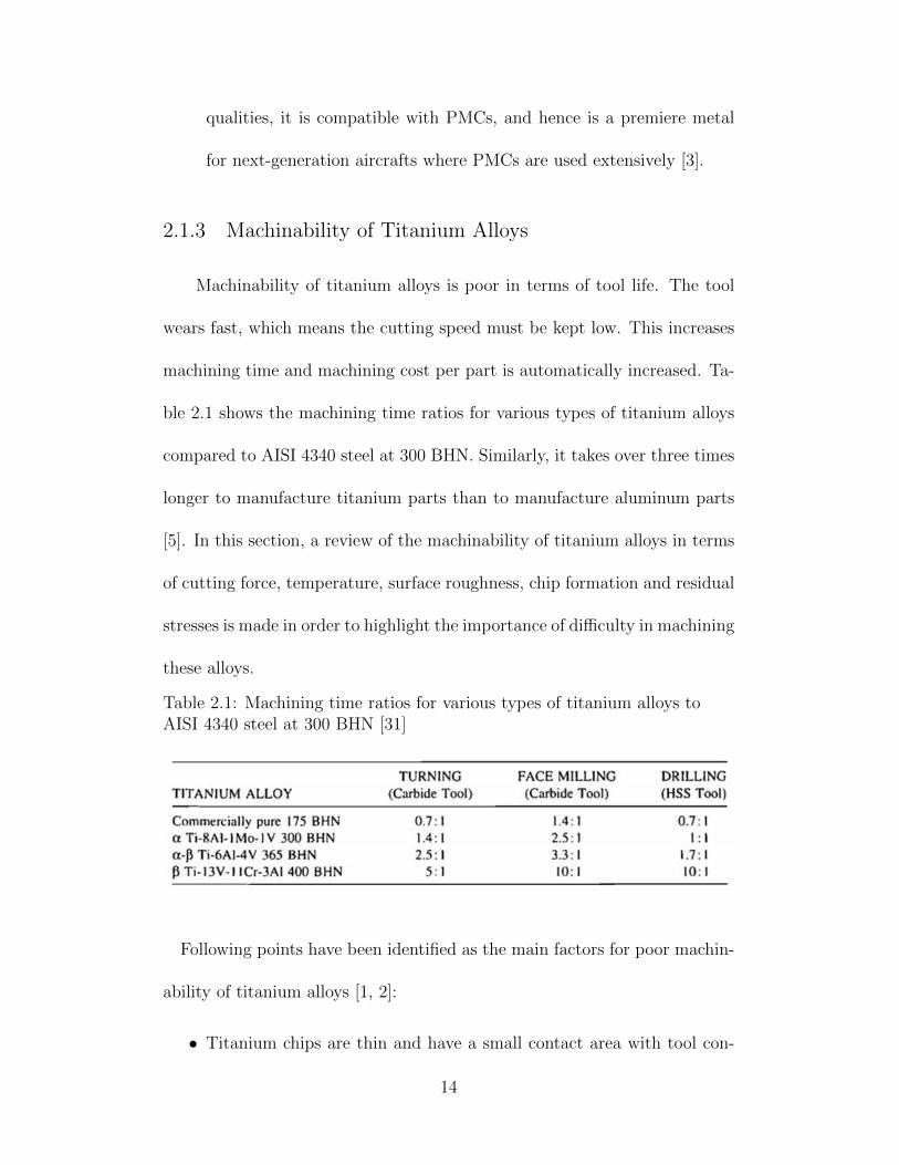
Table 2.1: Machining time ratios for various types of titanium alloys toAISI 4340 steel at 300 BHN [31]

Following points have been identified as the main factors for poor machin-

ability of titanium alloys [1, 2]:

• Titanium chips are thin and have a small contact area with tool con-

14

sequently. This causes high stresses in tool.

• Titanium has strong chemical affinity with most tool materials at tem-

peratures above 500oC.

• The catastrophic thermoplastic shear process by which chips are formed.

• Titanium has low modulus of elasticity which can cause chatter, de-

flection, and rubbing problems.

• Titanium has a tendency to ignite during machining due to high tem-

peratures involved.

Cutting Force

Studies on cutting force during machining of titanium alloys, namely Ti-

6Al-4V, have been conducted by various authors [32, 33, ?]. Experimental

results by Sun et al. [32] on turning of Ti-6Al-4V show that all the three

cutting conditions - feedrate, depth of cut and speed have influence on the

cutting force. Figure 2.1 shows that as the feed-rate is increased the cutting

force also increases in general. However, feed and thrust force components do

not vary as much as the cutting force. It has also been observed that there

is a variation in the amplitude of the cutting force and the oscillation is

prominent at lower feeds. This is attributed to the low modulus of elasticity

and high strength of titanium. With depth of cut the force also increases

(see Fig. 2.1) as tool is plunged further into the material. This causes wear

15

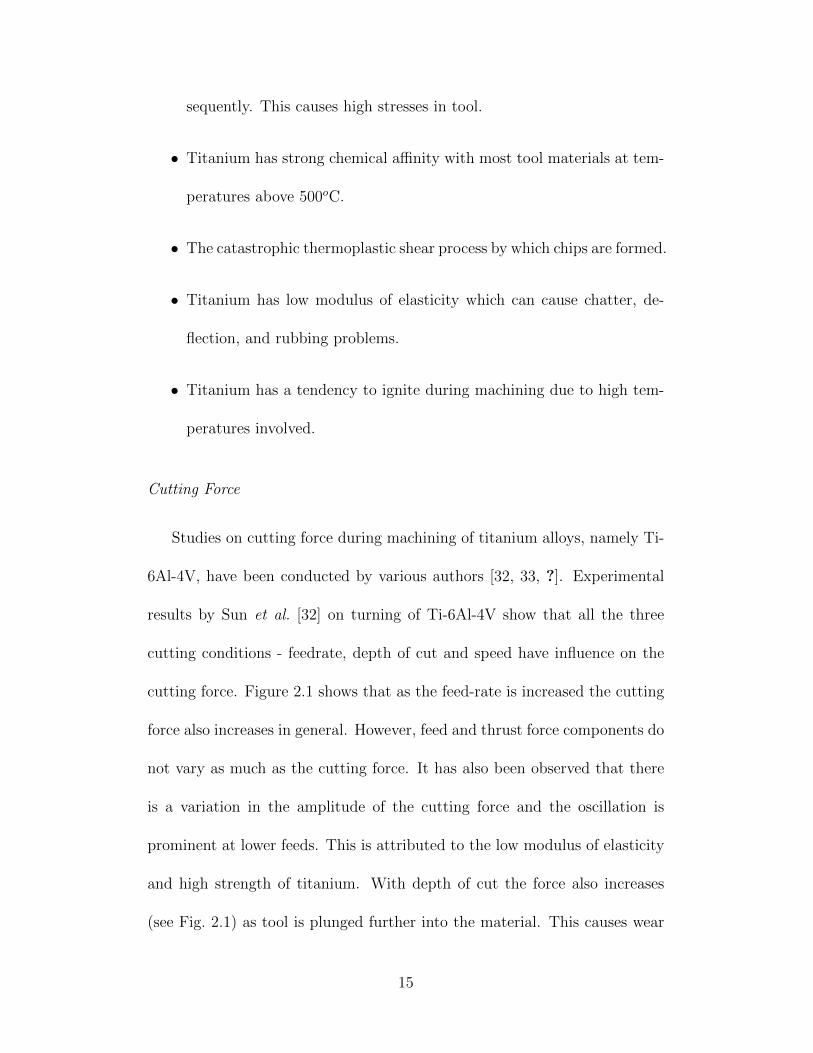
of the tool and affects the tool life.

Figure 2.1: Effect of feed and depth of cut on cutting force at cutting speedof 75 m/min) [32]

Increase in the average cutting speed show a general decrease in the cut-

ting force as observed by both Sun et al. [32] and Balaji et al. [33]. Results

from the works of Sun et al. (see Fig. 2.2) show that cutting force increases

initially with cutting speed up to 21 m/min due to strain hardening and

then decreases dramatically with cutting speed from 21 to 57 m/min. This

decrease is attributed to thermal softening due to the increased cutting tem-

perature, which requires less work for shear failure and hence, lower average

cutting forces. Therefore, the temperature sensitivity of the workpiece pre-

dominates over the strain rate sensitivity within the cutting speed range and

force is decreased. However, the increase in temperature is detrimental to the

tool and will cause rapid wear during machining at those cutting conditions.

16

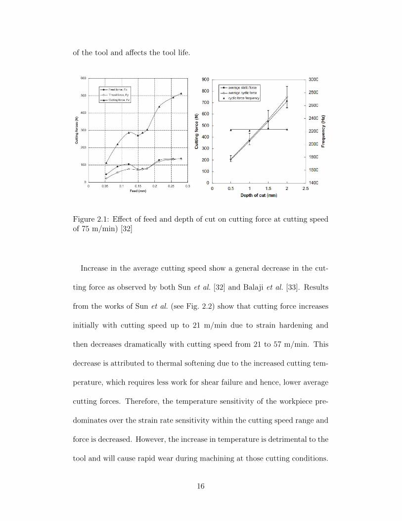
Figure 2.3 shows the effect of the cutting speed and feed on the tool life as

observed by Kahles et al. [34].

Figure 2.2: Effect of depth of cut and on cutting force at a cutting speed of16 m/min and feed of 0.280 mm ) [32]

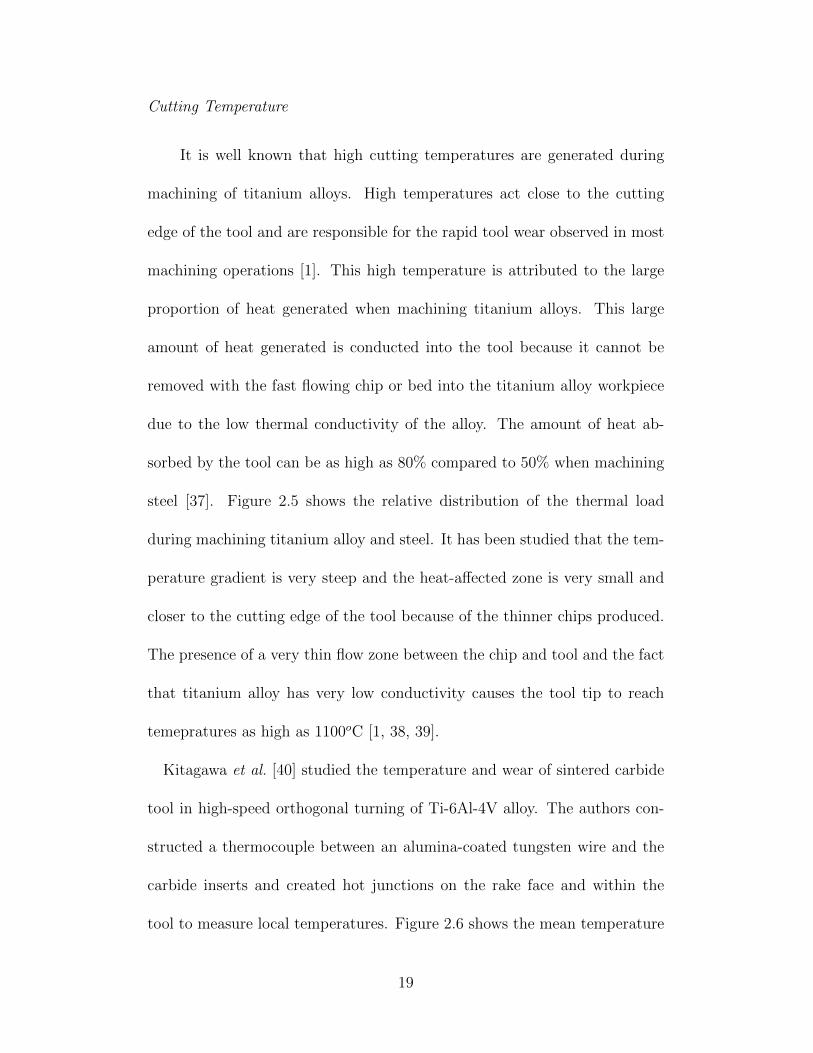
During milling, cutting forces can also be high, as observed by Shi et

al. [35] in their experimental study of the milling of a new damage-tolerant

titanium alloy (TC21). Their results are shown in Fig. 2.4. Vijay et al. [36]

also conducted experiments on end milling of Ti-6Al-4V and found similar

trend in cutting force with the increase in the depth of cut and feed rate.

This may be attributed to the unusually small chip-tool contact area on the

rake face when machining titanium.

17

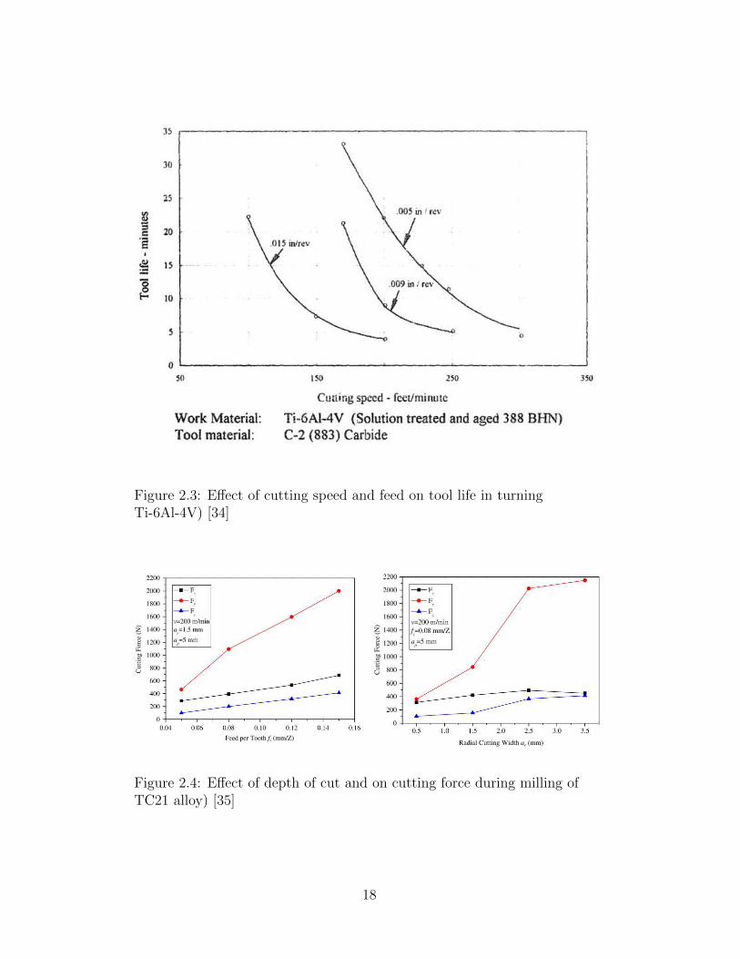
Figure 2.3: Effect of cutting speed and feed on tool life in turningTi-6Al-4V) [34]

Figure 2.4: Effect of depth of cut and on cutting force during milling ofTC21 alloy) [35]

18

Cutting Temperature

It is well known that high cutting temperatures are generated during

machining of titanium alloys. High temperatures act close to the cutting

edge of the tool and are responsible for the rapid tool wear observed in most

machining operations [1]. This high temperature is attributed to the large

proportion of heat generated when machining titanium alloys. This large

amount of heat generated is conducted into the tool because it cannot be

removed with the fast flowing chip or bed into the titanium alloy workpiece

due to the low thermal conductivity of the alloy. The amount of heat ab-

sorbed by the tool can be as high as 80% compared to 50% when machining

steel [37]. Figure 2.5 shows the relative distribution of the thermal load

during machining titanium alloy and steel. It has been studied that the tem-

perature gradient is very steep and the heat-affected zone is very small and

closer to the cutting edge of the tool because of the thinner chips produced.

The presence of a very thin flow zone between the chip and tool and the fact

that titanium alloy has very low conductivity causes the tool tip to reach

temepratures as high as 1100oC [1, 38, 39].

Kitagawa et al. [40] studied the temperature and wear of sintered carbide

tool in high-speed orthogonal turning of Ti-6Al-4V alloy. The authors con-

structed a thermocouple between an alumina-coated tungsten wire and the

carbide inserts and created hot junctions on the rake face and within the

tool to measure local temperatures. Figure 2.6 shows the mean temperature

19

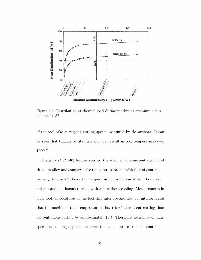
Figure 2.5: Distribution of thermal load during machining titanium alloysand steel) [37]

of the tool rake at varying cutting speeds measured by the authors. It can

be seen that turning of titanium alloy can result in tool temperatures over

1000oC.

Kitagawa et al. [40] further studied the effect of intermittent turning of

titanium alloy and compared the temperature profile with that of continuous

turning. Figure 2.7 shows the temperature data measured from both inter-

mittent and continuous turning with and without cooling. Measurements in

local tool temperatures at the tool-chip interface and the tool interior reveal

that the maximum rake temperature is lower for intermittent cutting than

for continuous cutting by approximately 15%. Therefore, feasibility of high-

speed end milling depends on lower tool temperatures than in continuous

20

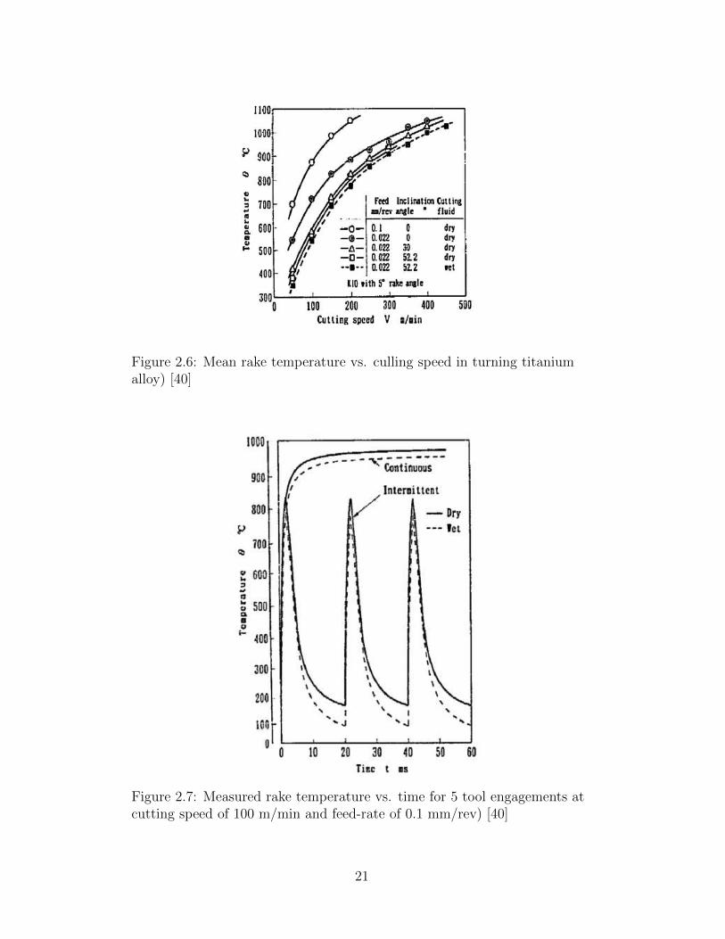
Figure 2.6: Mean rake temperature vs. culling speed in turning titaniumalloy) [40]

Figure 2.7: Measured rake temperature vs. time for 5 tool engagements atcutting speed of 100 m/min and feed-rate of 0.1 mm/rev) [40]

21

turning, owing to the time lag in temperature rise. Additionally, from this

study it is clear that an efficient cooling technique is essential for reduced

cutting temperature in turning of Ti-6Al-4V alloy and consequent longer tool

life.

Infact, it has been observed that cutting speed has the most considerable

influence on tool life; the tool life is extremely short at high cutting speeds but

improves dramatically as the speed is reduced [1]. At higher cutting speed,

thermal softening of the workpiece takes place as temperatures increase. This

increased temperature is responsible for thermal degradation of tool wear.

Surface Roughness

There are many methods to quantify the surface integrity of a ma-

chined part, and the most widely used method is the surface roughness. It

is considered to be the primary indicator of the quality of the surface fin-

ish [41]. The temperatures created during high-speed machining of titanium

alloy were found to play a major role in tool wear, which is a significant

factor in surface roughness of materials [40].

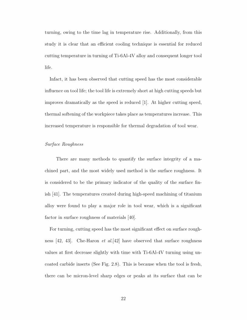
For turning, cutting speed has the most significant effect on surface rough-

ness [42, 43]. Che-Haron et al.[42] have observed that surface roughness

values at first decrease slightly with time with Ti-6Al-4V turning using un-

coated carbide inserts (See Fig. 2.8). This is because when the tool is fresh,

there can be micron-level sharp edges or peaks at its surface that can be

22

trimmed out to create a smoother contact surface with the workpiece as

cutting proceeds. However, as time goes by, the surface roughness values in-

crease sharply. This can be attributed to the deformation/wear of flank face

or adherence of workpiece material at tool nose. In addition to this, it has

been found that average surface roughness produced during machining using

tungsten carbide inserts is lower compared to that using PCD for speeds of

40-80m/min [43].

Figure 2.8: Typical surface roughness at feedrate of 0.35 mm/rev) [42]

Chip Morphology

Chip morphology and segmentation play a predominant role in deter-

mining the machinability of titanium alloy and tool wear. At lower cutting

speeds the chip is often discontinuous, while the chip becomes serrated as

the cutting speeds are increased [44]. Chip formation involves two fracture

mechanisms of work material [45], ductile fracture mechanism caused by over-

23

strain under compressive stress and high-speed ductile fracture mechanism

caused by strain concentration due to the local weakening by heat generation.

The titanium chips form saw-tooth shape as a consequence of a catastrophic

thermoplastic shear. This takes place when thermal softening in the primary

shear zone due to high heat generation during high-speed machining, is equal

or higher than the strain hardening produced by high strain rate. This leads

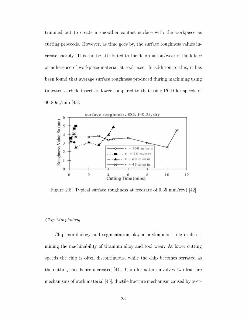
to the formation of the shear bands. Komanduri et al. [46] studied the chip

formation process during the cutting of Ti6Al4V and concluded that the

catastrophic shear chip exists in all speed ranges and is independent of tool

geometry. Figure 2.9 shows the segmented chips formed during machining of

Ti-6Al-4V alloy.

Figure 2.9: SEM images of cross-sectional top view of the major section ofthe chips at different cutting speeds. (a) 150 m/min. (b) 300 m/min. (c)450 m/min) [47]

24

2.2 Cutting Fluid Application Techniques used in

Machining

The high temperature and stresses developed at the cutting edge of the

tool are the main reasons for the difficult machinability of titanium alloys.

To address the problem, a cutting fluid needs to be applied as a basic rule.

The cutting fluid not only acts as a coolant but also as a lubricant that

reduces the tool friction and cutting forces, thus improving the tool life.

Uninterrupted flow of coolant can also provide a good flushing action to

remove chips and minimize the temperature. Additionally, a high pressure

coolant supply can result in discontinuous and easily disposable chips, as

opposed to the continuous chips produced in machining with conventional

cooling methods [1].

Palanisamy et al. [48] studied the effect of the application of cutting fluid

at high pressure during machining of titanium alloys. The authors observed

that using high-pressure coolant during machining results in longer tool life

and better surface finish on the machined material. Figure 2.10 shows that

application of high-pressure cooling (90 bar) increases machining time and

minimizes flank wear compared to low-pressure (6 bar) cooling. With low-

pressure cooling the excessive temperature at the chip-tool interface can re-

sult in the welding of chips to the insert (Fig. 2.10a). This results in signifi-

cant damage in the crater and flank section of the insert. This weakens the

cutting edge and results in the edge breakdown. In high-pressure cooling,

25

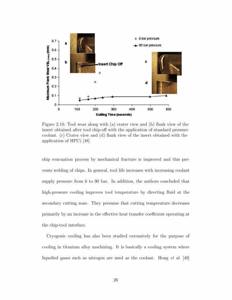
Figure 2.10: Tool wear along with (a) crater view and (b) flank view of theinsert obtained after tool chip-off with the application of standard pressurecoolant. (c) Crater view and (d) flank view of the insert obtained with theapplication of HPC) [48]

chip evacuation process by mechanical fracture is improved and this pre-

vents welding of chips. In general, tool life increases with increasing coolant

supply pressure from 6 to 90 bar. In addition, the authors concluded that

high-pressure cooling improves tool temperature by directing fluid at the

secondary cutting zone. They presume that cutting temperature decreases

primarily by an increase in the effective heat transfer coefficient operating at

the chip-tool interface.

Cryogenic cooling has also been studied extensively for the purpose of

cooling in titanium alloy machining. It is basically a cooling system where

liquefied gases such as nitrogen are used as the coolant. Hong et al. [49]

26

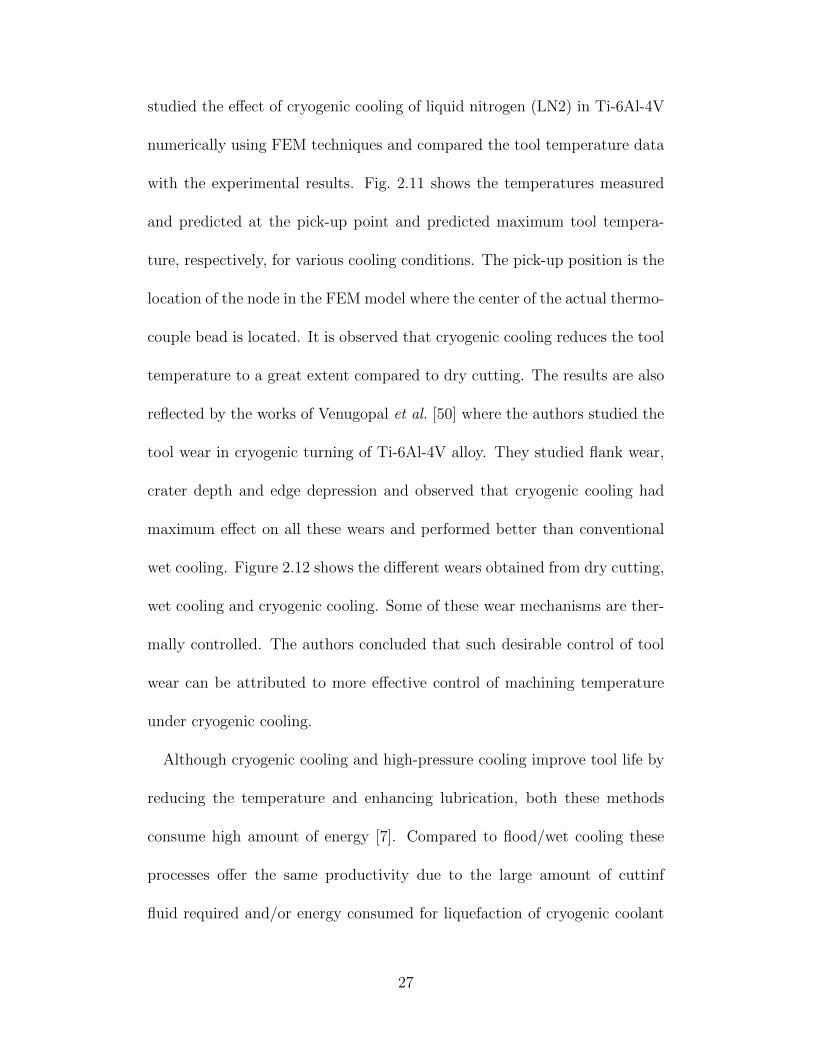
studied the effect of cryogenic cooling of liquid nitrogen (LN2) in Ti-6Al-4V

numerically using FEM techniques and compared the tool temperature data

with the experimental results. Fig. 2.11 shows the temperatures measured

and predicted at the pick-up point and predicted maximum tool tempera-

ture, respectively, for various cooling conditions. The pick-up position is the

location of the node in the FEM model where the center of the actual thermo-

couple bead is located. It is observed that cryogenic cooling reduces the tool

temperature to a great extent compared to dry cutting. The results are also

reflected by the works of Venugopal et al. [50] where the authors studied the

tool wear in cryogenic turning of Ti-6Al-4V alloy. They studied flank wear,

crater depth and edge depression and observed that cryogenic cooling had

maximum effect on all these wears and performed better than conventional

wet cooling. Figure 2.12 shows the different wears obtained from dry cutting,

wet cooling and cryogenic cooling. Some of these wear mechanisms are ther-

mally controlled. The authors concluded that such desirable control of tool

wear can be attributed to more effective control of machining temperature

under cryogenic cooling.

Although cryogenic cooling and high-pressure cooling improve tool life by

reducing the temperature and enhancing lubrication, both these methods

consume high amount of energy [7]. Compared to flood/wet cooling these

processes offer the same productivity due to the large amount of cuttinf

fluid required and/or energy consumed for liquefaction of cryogenic coolant

27

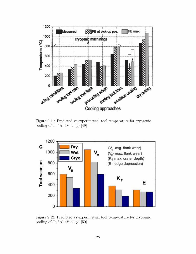
Figure 2.11: Predicted vs experimetnal tool temperature for cryogeniccooling of Ti-6Al-4V alloy) [49]

Figure 2.12: Predicted vs experimetnal tool temperature for cryogeniccooling of Ti-6Al-4V alloy) [50]

28

and for pumping high-pressure coolant. As a result, an alternative form

of cooling method has recently been developed that consumes less energy

and reduces the cutting temperature at the same time [9]. The new cooling

method, known as the atomization-based cutting-fluid (ACF) spray system,

has helped in reducing the tool temperature during machining [10] and has

improved tool life by 40-50% over flood cooling [7]. A combination of spray

system parameters used in the ACF spray system has shown improved ma-

chining performance such as tool life, cutting force, and chip breakability

during titanium machining [7]. More details on the ACF spray system as

one of the alternative cooling technologies is described in the next section.

2.3 ACF Spray System

The atomization-based cutting fluid (ACF) spray system was first pro-

posed as an efficient cooling technique for micromachining [8]. Hoyne et

al. [10] and Nath et al. [7] later showed that ACF spray system is able to

successfully reduce the overall temperature of the tool and increase tool lifes-

pan during turning of titanium alloys. In the study by Nath et al. [7], the

ACF spray system was observed to reduce friction coefficient at the cutting

interface, and improve tool life and surface finish during machining. Hoyne et

al. [9] further studied the film that is formed after the spray from the ACF

spray system impinges on the surface. From the study, it was established

that there are three zones of film and the steady film zone is the most suit-

29

able for the cutting interface in machining for lubrication and temperature

reduction. In addition, it was also observed experimentally in another study

by the same authors [10] that the ACF spray system is able to reduce the

tool temperature successfully.

2.3.1 ACF Spray System Components

The ACF spray system schematic is shown in Fig. 2.13. It consists of a

cutting fluid reservoir, an ultrasonic atomizer, two coaxial nozzles of different

diameters, and a gas supply system. The ultrasonic atomizer at one end that

generates monodispersed spray droplets (e.g. ∼ 10−100 µm). There are two

coaxial nozzles in the system, the droplet nozzle and the gas nozzle. The low-

velocity droplets formed from the atomizer flow through the larger droplet

nozzle that are then entrained by the high-velocity gas (e.g. air and/or

CO2) flowing through the inner gas nozzle. The entrainment is created by

the pressure drop around the gas jet that draws in the droplets and carry

them forward. This produces a focused axisymmetric jet of droplets that are

impinged at the tool-chip interface. Upon impingement, the droplets interact

with the heated tool/chip surface leading to heat transfer and vaporization

of droplets that results in cooling of the tool/chip surface.

30

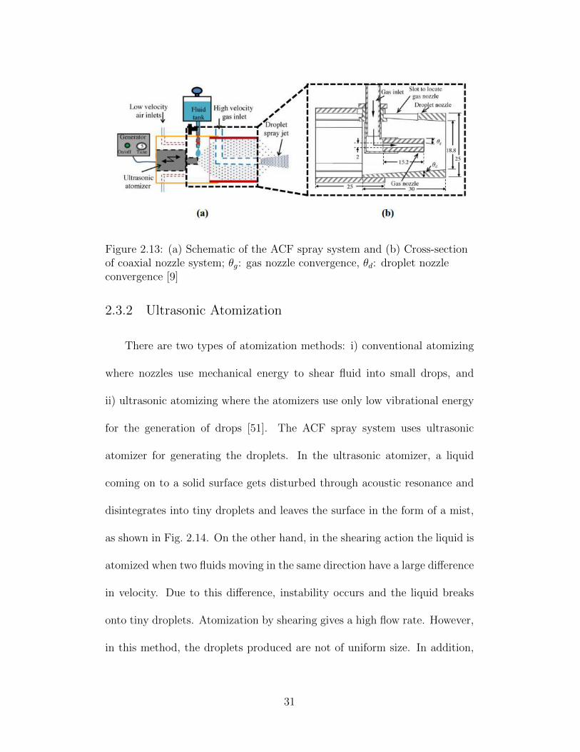
Figure 2.13: (a) Schematic of the ACF spray system and (b) Cross-sectionof coaxial nozzle system; θg: gas nozzle convergence, θd: droplet nozzleconvergence [9]

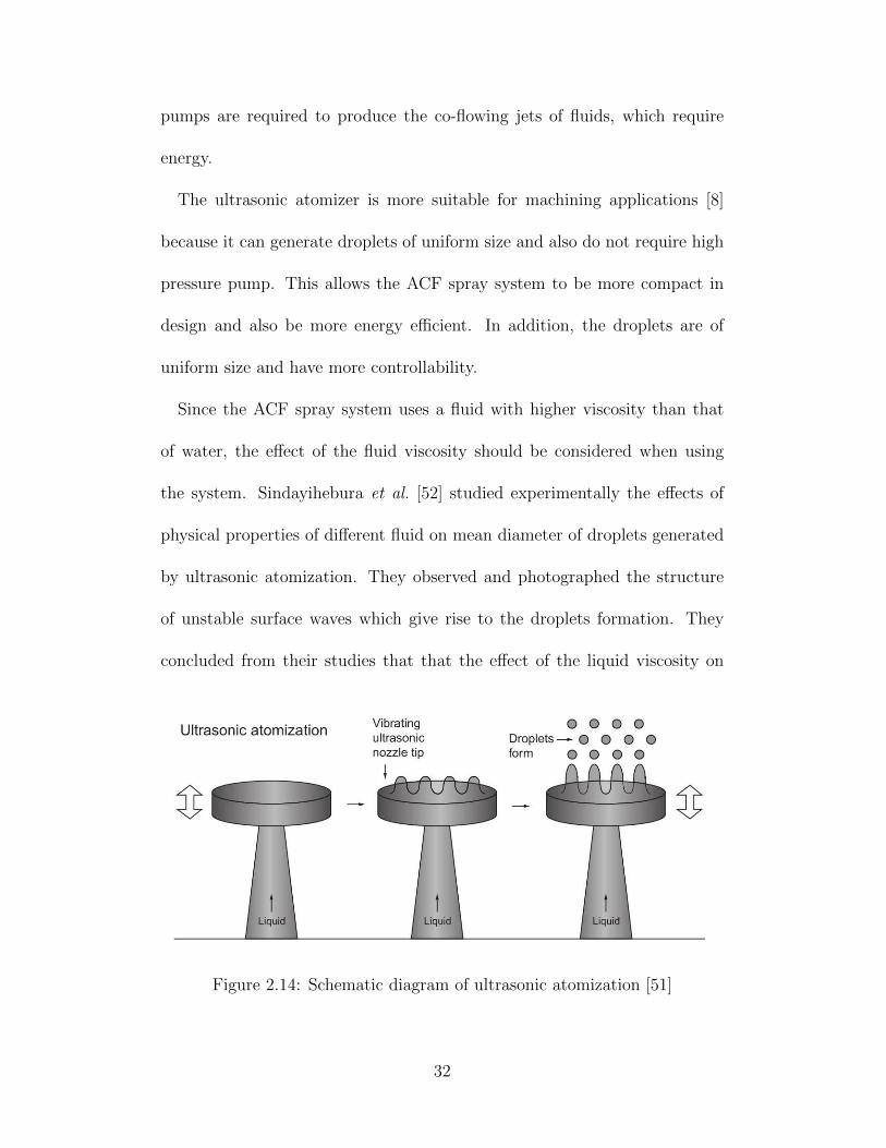
2.3.2 Ultrasonic Atomization

There are two types of atomization methods: i) conventional atomizing

where nozzles use mechanical energy to shear fluid into small drops, and

ii) ultrasonic atomizing where the atomizers use only low vibrational energy

for the generation of drops [51]. The ACF spray system uses ultrasonic

atomizer for generating the droplets. In the ultrasonic atomizer, a liquid

coming on to a solid surface gets disturbed through acoustic resonance and

disintegrates into tiny droplets and leaves the surface in the form of a mist,

as shown in Fig. 2.14. On the other hand, in the shearing action the liquid is

atomized when two fluids moving in the same direction have a large difference

in velocity. Due to this difference, instability occurs and the liquid breaks

onto tiny droplets. Atomization by shearing gives a high flow rate. However,

in this method, the droplets produced are not of uniform size. In addition,

31

pumps are required to produce the co-flowing jets of fluids, which require

energy.

The ultrasonic atomizer is more suitable for machining applications [8]

because it can generate droplets of uniform size and also do not require high

pressure pump. This allows the ACF spray system to be more compact in

design and also be more energy efficient. In addition, the droplets are of

uniform size and have more controllability.

Since the ACF spray system uses a fluid with higher viscosity than that

of water, the effect of the fluid viscosity should be considered when using

the system. Sindayihebura et al. [52] studied experimentally the effects of

physical properties of different fluid on mean diameter of droplets generated

by ultrasonic atomization. They observed and photographed the structure

of unstable surface waves which give rise to the droplets formation. They

concluded from their studies that that the effect of the liquid viscosity on

Figure 2.14: Schematic diagram of ultrasonic atomization [51]

32

the droplet mean diameter is insignificant. However, the effect of viscosity is

significant for impingement characteristics as the droplets interact with the

surface.

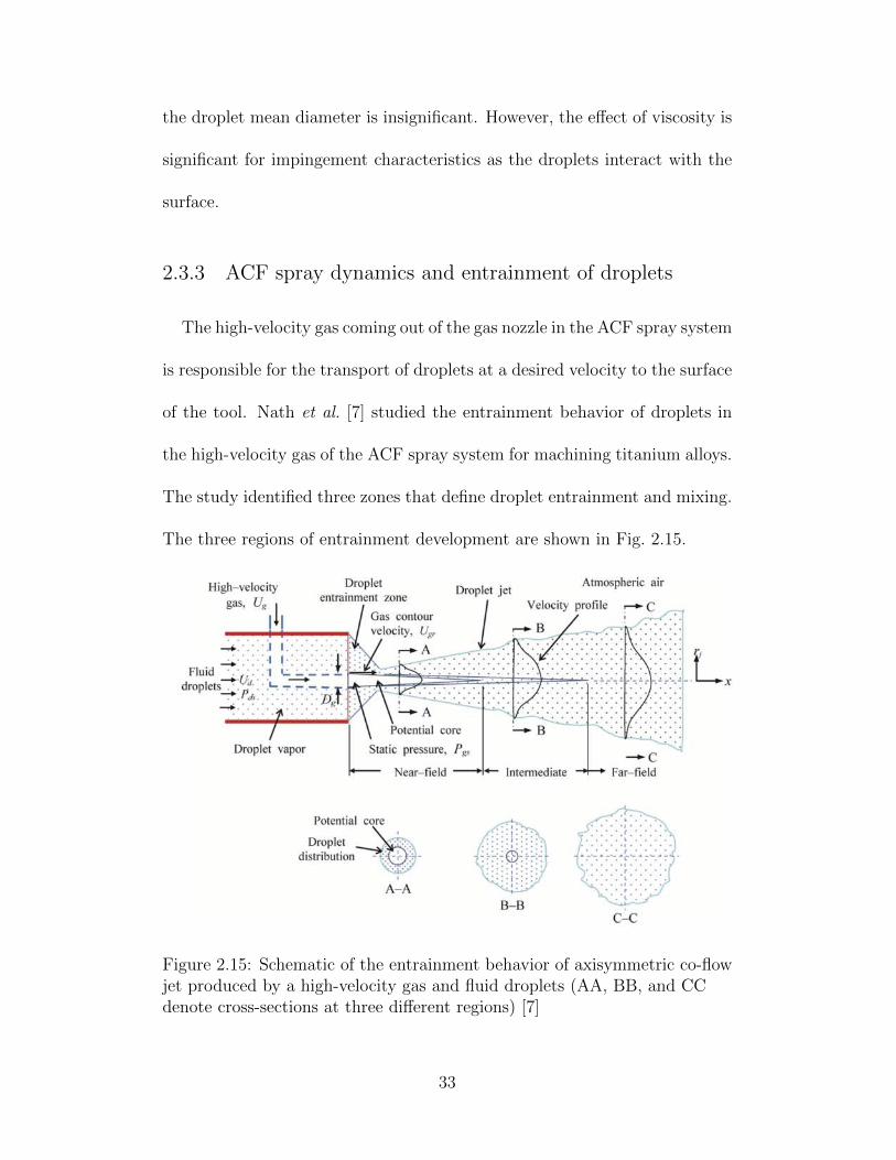
2.3.3 ACF spray dynamics and entrainment of droplets

The high-velocity gas coming out of the gas nozzle in the ACF spray system

is responsible for the transport of droplets at a desired velocity to the surface

of the tool. Nath et al. [7] studied the entrainment behavior of droplets in

the high-velocity gas of the ACF spray system for machining titanium alloys.

The study identified three zones that define droplet entrainment and mixing.

The three regions of entrainment development are shown in Fig. 2.15.

Figure 2.15: Schematic of the entrainment behavior of axisymmetric co-flowjet produced by a high-velocity gas and fluid droplets (AA, BB, and CCdenote cross-sections at three different regions) [7]

33

In the first region called the near-field (NF) zone, a potential core is ob-

served with the absence of any droplet generated by the ultrasonic atomizer.

In this NF region, the vorticity is zero and as a result, no mixing of the fluids

occurs. On the other hand, the droplets are distributed uniformly in the

FF zone. In between the NF and the FF zone the droplets get entrained by

the high-velocity gas. For the different conditions studied, the authors have

reported that uniform distribution takes place at 25-35 mm or at x/Dg >16.

They have also observed that when droplet velocity increases and gas veloc-

ity decreases, the distance between the gas nozzle exit and the FF region

becomes smaller. Finally, the authors concluded that having the spray dis-

tance outside the potential core ensured an even distribution of droplets and

consequently an even fluid film formation in machining. Thus, a larger spray

distance reduces friction coefficient at the cutting interface, and improves

tool life and surface finish during machining.

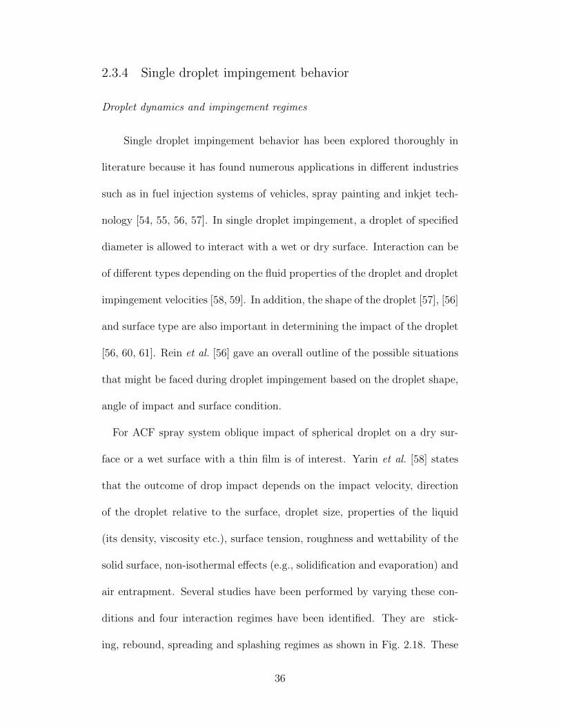
Rukosuyev et al. [53] studied the effects of system parameters on ultra-

sonic cutting fluid application system in micro-machining. In this study the

authors evaluated the focusing capability of the generated spray and the ef-

fects of different nozzle geometries and spray parameters (spray velocity).

Figure 2.16 shows the different positions of the gas nozzle with respect to

the droplet nozzle and Fig. 2.17 shows the resulting spray at those geome-

tries and spray parameters (see Fig. 2.17 for the spray parameters). They

concluded that the position of the nozzle with respect to the cutting zone is

34

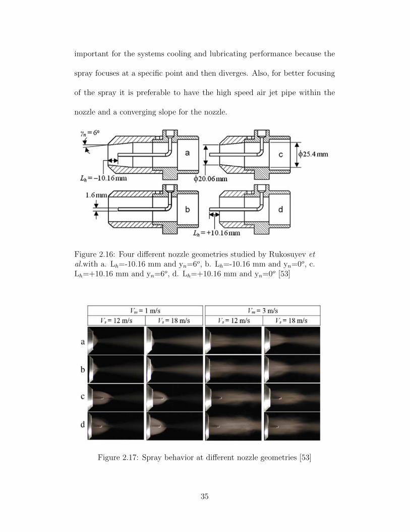
important for the systems cooling and lubricating performance because the

spray focuses at a specific point and then diverges. Also, for better focusing

of the spray it is preferable to have the high speed air jet pipe within the

nozzle and a converging slope for the nozzle.

Figure 2.16: Four different nozzle geometries studied by Rukosuyev etal.with a. Lh=-10.16 mm and yn=6o, b. Lh=-10.16 mm and yn=0o, c.Lh=+10.16 mm and yn=6o, d. Lh=+10.16 mm and yn=0o [53]

Figure 2.17: Spray behavior at different nozzle geometries [53]

35

2.3.4 Single droplet impingement behavior

Droplet dynamics and impingement regimes

Single droplet impingement behavior has been explored thoroughly in

literature because it has found numerous applications in different industries

such as in fuel injection systems of vehicles, spray painting and inkjet tech-

nology [54, 55, 56, 57]. In single droplet impingement, a droplet of specified

diameter is allowed to interact with a wet or dry surface. Interaction can be

of different types depending on the fluid properties of the droplet and droplet

impingement velocities [58, 59]. In addition, the shape of the droplet [57], [56]

and surface type are also important in determining the impact of the droplet

[56, 60, 61]. Rein et al. [56] gave an overall outline of the possible situations

that might be faced during droplet impingement based on the droplet shape,

angle of impact and surface condition.

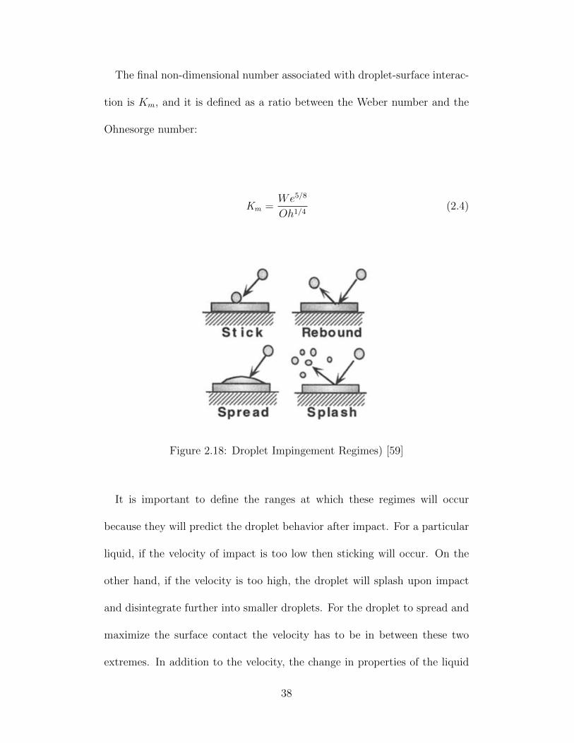
For ACF spray system oblique impact of spherical droplet on a dry sur-

face or a wet surface with a thin film is of interest. Yarin et al. [58] states

that the outcome of drop impact depends on the impact velocity, direction

of the droplet relative to the surface, droplet size, properties of the liquid

(its density, viscosity etc.), surface tension, roughness and wettability of the

solid surface, non-isothermal effects (e.g., solidification and evaporation) and

air entrapment. Several studies have been performed by varying these con-

ditions and four interaction regimes have been identified. They are stick-

ing, rebound, spreading and splashing regimes as shown in Fig. 2.18. These

36

regimes can be characterized by several non-dimensional numbers. These

include: Reynolds number (Re), Ohnesorge number (Oh), Weber number

(We) and non-dimensional number, Km. Reynolds number Re is the ratio

of the inertial force by viscous force and is characterized by,

Re =ρvdd0µ

, (2.1)

where ρ is the density and is the dynamic viscosity of the fluid. The

term d0 represents characteristic length and vd the impact velocity of the

droplet. Ohnesorge number gives the relation between the inertial, viscous

and surface tension forces and is given by,

Oh =µ√ρσd0

, (2.2)

where σ is the surface tension of the liquid droplet. Weber number is

defined as the ration of the droplet kinetic energy to the droplet surface

energy and is mathematically written as:

We =ρvd

2d0σ

(2.3)

37

The final non-dimensional number associated with droplet-surface interac-

tion is Km, and it is defined as a ratio between the Weber number and the

Ohnesorge number:

Km =We5/8

Oh1/4(2.4)

Figure 2.18: Droplet Impingement Regimes) [59]

It is important to define the ranges at which these regimes will occur

because they will predict the droplet behavior after impact. For a particular

liquid, if the velocity of impact is too low then sticking will occur. On the

other hand, if the velocity is too high, the droplet will splash upon impact

and disintegrate further into smaller droplets. For the droplet to spread and

maximize the surface contact the velocity has to be in between these two

extremes. In addition to the velocity, the change in properties of the liquid

38

will also affect the droplet impact regime. Based on these parameters, the

non-dimensionless numbers discussed above will have ranges for which these

regimes occur.

For the stick regime to occur, the Weber number needs to be less than 5,

as reported by Jayaratne et al. [62], who studied the sticking regime of water

droplets on wetted surface experimentally by varying the droplet diameter,

velocity and impingement angle. Above this Weber number, rebound will

take place. The rebound regime for water droplets on a fixed wetted surface

is 5 < We < 10, as reported by Stow et al. [63]. Above Weber number

of 10, spreading occurs. This regime is of interest in ACF spray system

cooling, since the droplet in this regime spreads to form maximum contact

with the surface and can contribute to higher heat transfer rate. With higher

impact energy the droplet breaks up into further smaller diameter droplets

and splashing occurs. To distinguish between the spreading and the splashing

regime the non-dimensionless number, Km is used. Mundo et al. [64] used

LED visualization technique to perform droplet impact tests on two different

steel surfaces and developed the non-dimensional number Km. The authors

determined that the droplet will spread if Km < 57.7 and splash otherwise

(See Fig. 2.19).

For a surface at a temperature above Leidenfrost temperature of the liquid

being used, the droplet may also break up or rebound and break up induced

by boiling as stated by Bai et al. [65]. At such high temperatures, partial

39

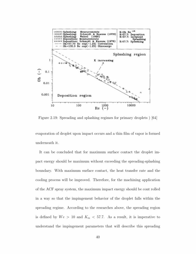
Figure 2.19: Spreading and splashing regimes for primary droplets ) [64]

evaporation of droplet upon impact occurs and a thin film of vapor is formed

underneath it.

It can be concluded that for maximum surface contact the droplet im-

pact energy should be maximum without exceeding the spreading-splashing

boundary. With maximum surface contact, the heat transfer rate and the

cooling process will be improved. Therefore, for the machining application

of the ACF spray system, the maximum impact energy should be cont rolled

in a way so that the impingement behavior of the droplet falls within the

spreading regime. According to the researches above, the spreading region

is defined by We > 10 and Km < 57.7. As a result, it is imperative to

understand the impingement parameters that will describe this spreading

40

regime.

Modeling of the spreading of single droplet and spray impingement

A number of researchers have worked on modeling the dynamics of

single droplet impingement. These studies are focused on the mechanism

of crown formation and generation of secondary droplets. This is expected

since there are a number of applications where splashing and consequent

atomization of droplets are important, such as fuel spray inside combustion

chambers [64, 66]. During ACF spray cooling, the droplet should spread with

the highest energy without exceeding the spreading/splashing boundary so

that maximum amount of area for the spreading is covered and droplets

penetrate the chip-tool interface. Fukai et al. [67] created a model of an im-

pinging droplet on a flat dry surface using mass continuity and momentum

equations for a long time scale (greater than 1 second). In the model the

authors studied the deformation of the droplet by accounting for the pres-

ence of inertial, viscous, gravitational, surface- tension, and wetting effects,

including the phenomenon of contact-angle hysteresis. Experiments were

also performed for a water droplet system in which impingement surfaces of

different wettability were employed. The contact angles determined experi-

mentally were used as input to the numerical model. The authors concluded

that the theoretical model predicted well the deformation of the impacting

droplet both during spreading and recoiling.

41

Ghai et al. [68] created a model of a spreading droplet during impact with

a dry rotating surface by using conservation of energy and volume in a mod-

ified spherical cap approach. The authors also extended the work for oblique

impacts on stationary dry surface by taking the tangential component of the

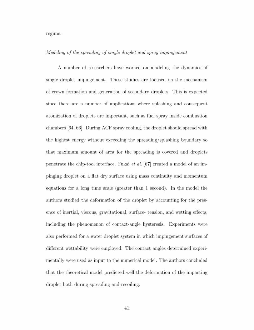
impact velocity on the surface. Yarin et al. [69] modeled droplet impact

behavior on a thin liquid film for weak impacts (We < 40) and established

that crowning does not occur at low We numbers. Instead, the droplet upon

impact on wetted surface at much longer times (of the order of 10−2 s) pro-

duces spreading patterns. A doughnut-like wave with a rim as shown in

Figure 2.20 represents such a pattern of inertial spreading counteracted by

surface tension.

Figure 2.20: Evolution of droplet spread for We=20 and at times 0, 0.1, 0.2,0.3, and 0.4 sec) [69]

42

Modeling of the ACF Spray Impingement

Since the ACF spray system is relatively a new technology, few works

have been done regarding the modeling of the system to characterize and

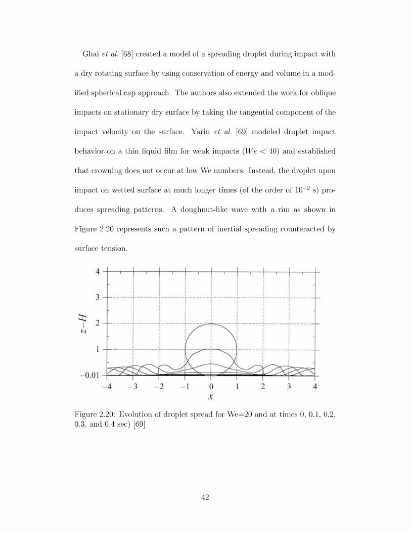
understand its operation. Hoyne et al. [9] developed a 3D thin fluid film

model for the ACF spray system based on the NavierStokes equations for

mass and momentum to predict the film thickness as it approaches the cut-

ting interface. The model takes into account of the cross-film velocity profile,

droplet impingement, pressure distributions and gasliquid shear interaction.

The authors also measured the film thickness experimentally by using fluo-

rescent dye and camera and identified three three distinct zones of the fluid

film created by the ACF spray system: (1) impingement zone; (2) steady

zone; and (3) unsteady zone. The three zones are shown in Fig. 2.21. The

impingement zone features a fast moving unsteady thin film that is due to

the disturbance of the high-velocity gas. The zone appears for a distance

from point of impingement (DIP) of less than 3 mm. Beyond the impinge-

ment zone, the film reaches the steady zone, which features thickness values

between 10 and 50 mm. After 7 mm, the film transitions to the unsteady

zone and becomes rougher as waviness and wisps develop on the film surface.

It was concluded from the experiments that the film present in the steady

zone is the least disturbed and therefore, most desirable of the three zones

at the chip-tool interface. The model developed the steady zone of the film,

and it was found that the film thickness was comparable to the experimental

43

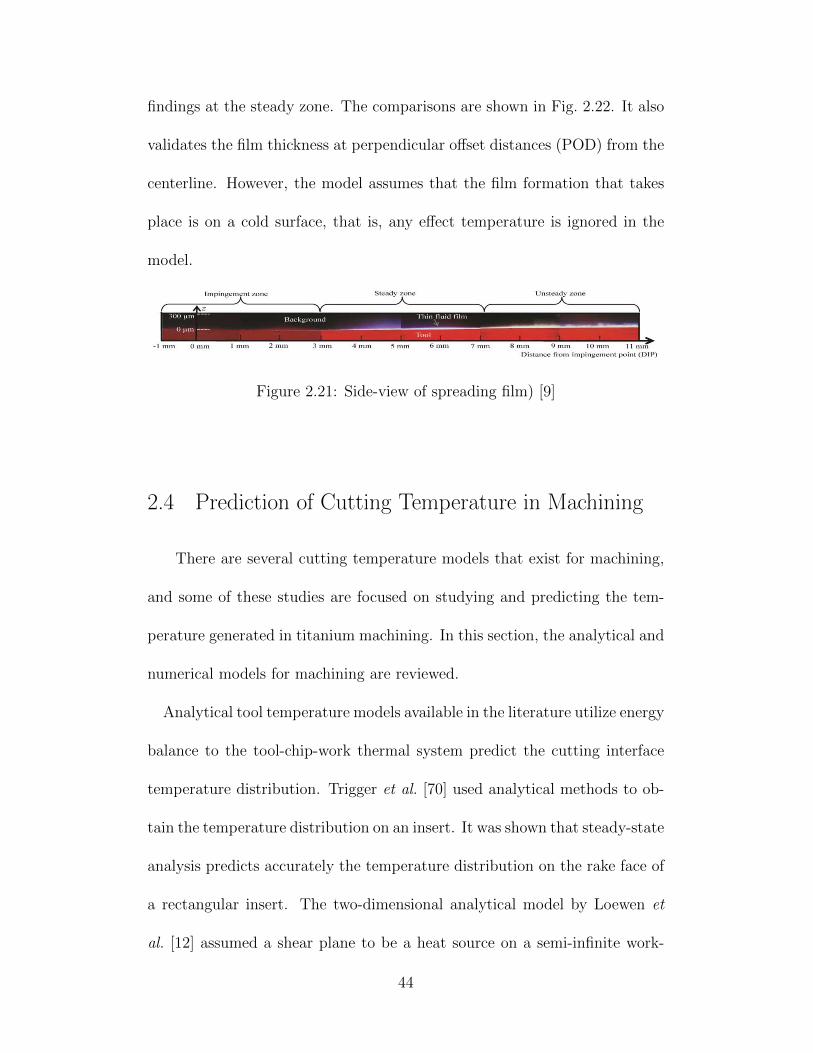
findings at the steady zone. The comparisons are shown in Fig. 2.22. It also

validates the film thickness at perpendicular offset distances (POD) from the

centerline. However, the model assumes that the film formation that takes

place is on a cold surface, that is, any effect temperature is ignored in the

model.

Figure 2.21: Side-view of spreading film) [9]

2.4 Prediction of Cutting Temperature in Machining

There are several cutting temperature models that exist for machining,

and some of these studies are focused on studying and predicting the tem-

perature generated in titanium machining. In this section, the analytical and

numerical models for machining are reviewed.

Analytical tool temperature models available in the literature utilize energy

balance to the tool-chip-work thermal system predict the cutting interface

temperature distribution. Trigger et al. [70] used analytical methods to ob-

tain the temperature distribution on an insert. It was shown that steady-state

analysis predicts accurately the temperature distribution on the rake face of

a rectangular insert. The two-dimensional analytical model by Loewen et

al. [12] assumed a shear plane to be a heat source on a semi-infinite work-

44

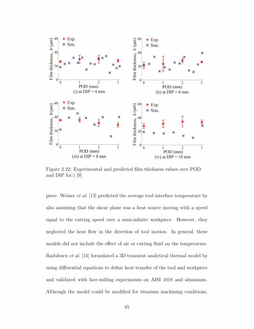
Figure 2.22: Experimental and predicted film thickness values over PODand DIP for:) [9]

piece. Weiner et al. [13] predicted the average tool interface temperature by

also assuming that the shear plane was a heat source moving with a speed

equal to the cutting speed over a semi-infinite workpiece. However, they

neglected the heat flow in the direction of tool motion. In general, these

models did not include the effect of air or cutting fluid on the temperature.

Radulescu et al. [14] formulated a 3D transient analytical thermal model by

using differential equations to define heat transfer of the tool and workpiece

and validated with face-milling experiments on AISI 1018 and aluminum.

Although the model could be modified for titanium machining conditions,

45

it also suffered the limitation of overlooking any fluid interaction with the

cutting interface.

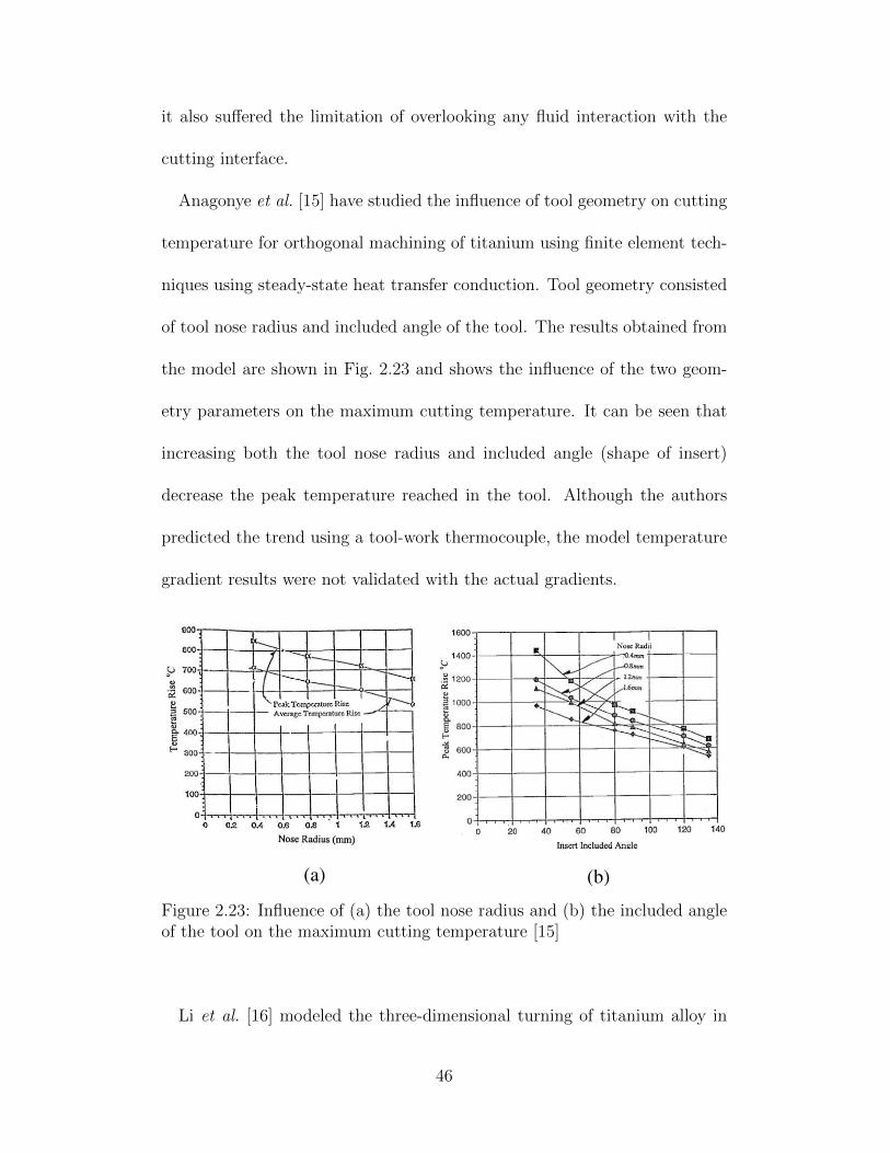
Anagonye et al. [15] have studied the influence of tool geometry on cutting

temperature for orthogonal machining of titanium using finite element tech-

niques using steady-state heat transfer conduction. Tool geometry consisted

of tool nose radius and included angle of the tool. The results obtained from

the model are shown in Fig. 2.23 and shows the influence of the two geom-

etry parameters on the maximum cutting temperature. It can be seen that

increasing both the tool nose radius and included angle (shape of insert)

decrease the peak temperature reached in the tool. Although the authors

predicted the trend using a tool-work thermocouple, the model temperature

gradient results were not validated with the actual gradients.

(a) (b)

Figure 2.23: Influence of (a) the tool nose radius and (b) the included angleof the tool on the maximum cutting temperature [15]

Li et al. [16] modeled the three-dimensional turning of titanium alloy in

46

the commercially available AdvantEdge 3D simulation software. The work-

material model in finite element analysis consists of the power-law strain

hardening, thermal softening, and rate sensitivity. The authors investigated

the effects of cutting speed on peak tool temperature and tool cutting edge

radius on forces, chip thickness, and tool temperature. Six finite element

simulations at two feeds and four cutting speeds were run to obtain the peak

temperature on the tool rake face. The peak tool temperature data is shown

in Fig. 2.24. Results show the temperature is independent of the feed and

has a direct correlation with cutting speed. They also studied the effect of

tool edge radius on the maximum temperature through the simulations. The

results shown in Fig. 2.25 indicate that with increase in the tool edge radius,

the peak temperature decreases. However, the authors did not validate any

of the temperature profiles predicted in their work. They also generated

chip temperature from the model by assuming that maximum chip and tool

temperatures are same as they are in contact with one another.

A finite element study using Johnson-Cook (JC) model was performed

by Karpat et al. [18] to predict the temperature of the chip. The study

investigates the influence of various flow softening conditions on the finite

element simulation outputs for machining titanium alloy Ti-6Al-4V. A new

flow softening expression, which allows defining temperature-dependent flow

softening behavior, is also proposed by the authors. In the model, assumption

of rigid tool is maintained. Figure 2.26 shows the temperature contour of the

47

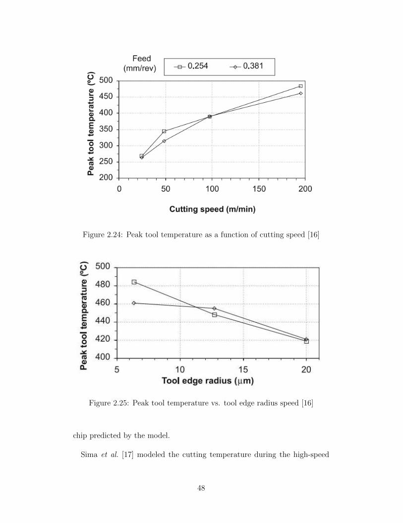
Figure 2.24: Peak tool temperature as a function of cutting speed [16]

Figure 2.25: Peak tool temperature vs. tool edge radius speed [16]

chip predicted by the model.

Sima et al. [17] modeled the cutting temperature during the high-speed

48

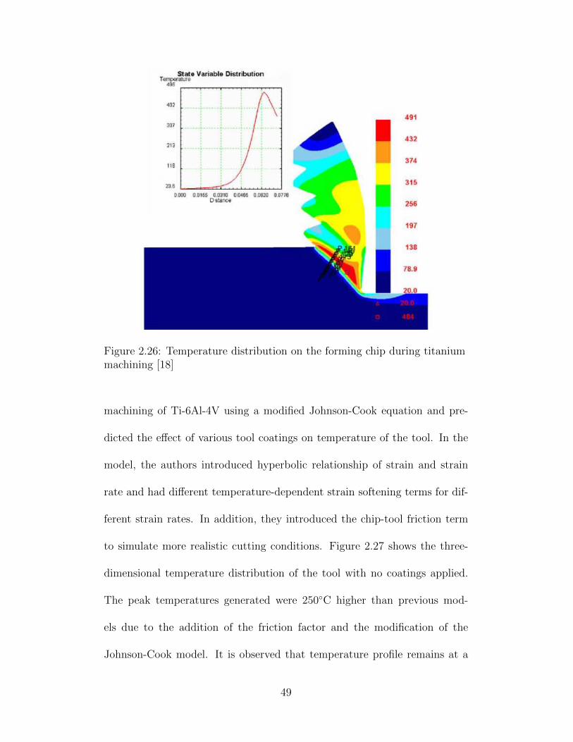
Figure 2.26: Temperature distribution on the forming chip during titaniummachining [18]

machining of Ti-6Al-4V using a modified Johnson-Cook equation and pre-

dicted the effect of various tool coatings on temperature of the tool. In the

model, the authors introduced hyperbolic relationship of strain and strain

rate and had different temperature-dependent strain softening terms for dif-

ferent strain rates. In addition, they introduced the chip-tool friction term

to simulate more realistic cutting conditions. Figure 2.27 shows the three-

dimensional temperature distribution of the tool with no coatings applied.

The peak temperatures generated were 250◦C higher than previous mod-

els due to the addition of the friction factor and the modification of the

Johnson-Cook model. It is observed that temperature profile remains at a

49

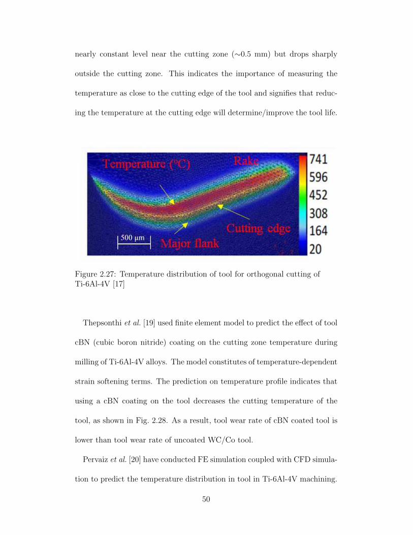
nearly constant level near the cutting zone (∼0.5 mm) but drops sharply

outside the cutting zone. This indicates the importance of measuring the

temperature as close to the cutting edge of the tool and signifies that reduc-

ing the temperature at the cutting edge will determine/improve the tool life.

Figure 2.27: Temperature distribution of tool for orthogonal cutting ofTi-6Al-4V [17]

Thepsonthi et al. [19] used finite element model to predict the effect of tool

cBN (cubic boron nitride) coating on the cutting zone temperature during

milling of Ti-6Al-4V alloys. The model constitutes of temperature-dependent

strain softening terms. The prediction on temperature profile indicates that

using a cBN coating on the tool decreases the cutting temperature of the

tool, as shown in Fig. 2.28. As a result, tool wear rate of cBN coated tool is

lower than tool wear rate of uncoated WC/Co tool.

Pervaiz et al. [20] have conducted FE simulation coupled with CFD simula-

tion to predict the temperature distribution in tool in Ti-6Al-4V machining.

50

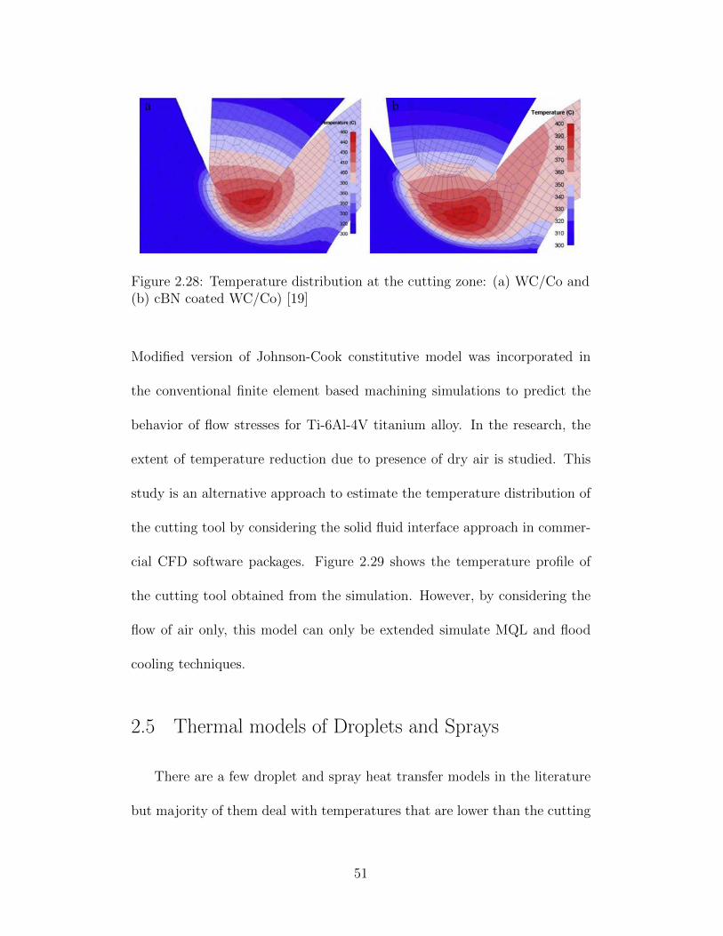
Figure 2.28: Temperature distribution at the cutting zone: (a) WC/Co and(b) cBN coated WC/Co) [19]

Modified version of Johnson-Cook constitutive model was incorporated in

the conventional finite element based machining simulations to predict the

behavior of flow stresses for Ti-6Al-4V titanium alloy. In the research, the

extent of temperature reduction due to presence of dry air is studied. This

study is an alternative approach to estimate the temperature distribution of

the cutting tool by considering the solid fluid interface approach in commer-

cial CFD software packages. Figure 2.29 shows the temperature profile of

the cutting tool obtained from the simulation. However, by considering the

flow of air only, this model can only be extended simulate MQL and flood

cooling techniques.

2.5 Thermal models of Droplets and Sprays

There are a few droplet and spray heat transfer models in the literature

but majority of them deal with temperatures that are lower than the cutting

51

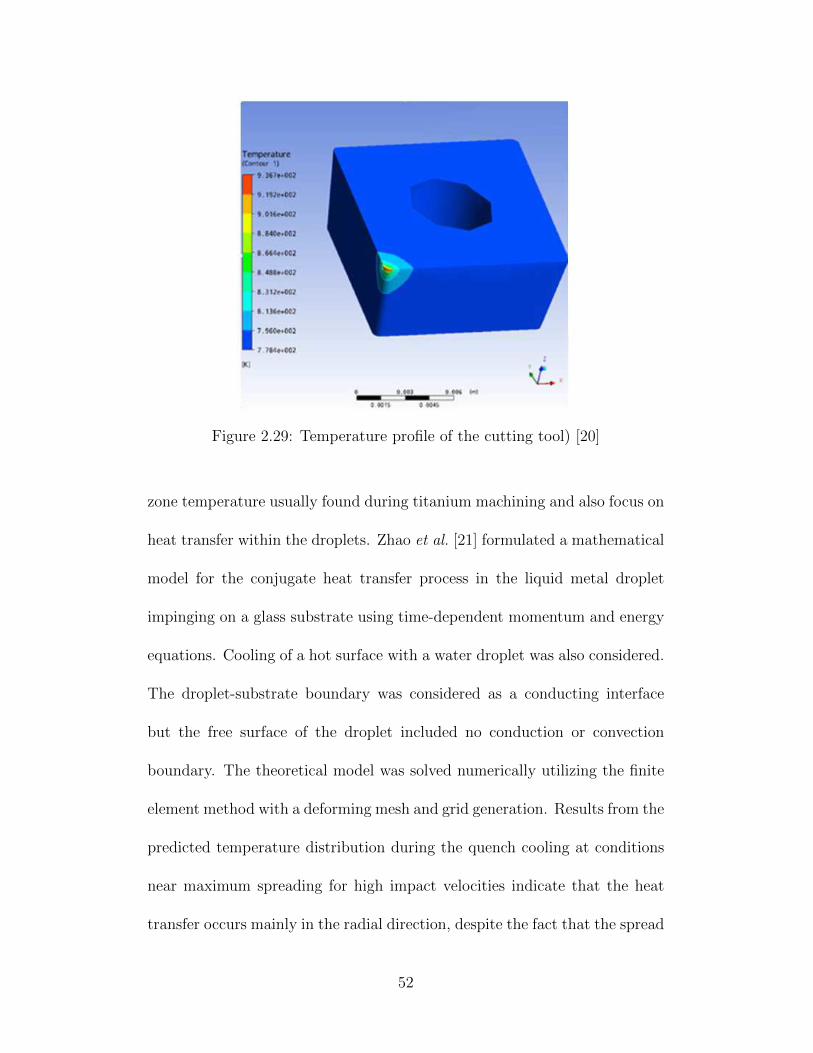
Figure 2.29: Temperature profile of the cutting tool) [20]

zone temperature usually found during titanium machining and also focus on

heat transfer within the droplets. Zhao et al. [21] formulated a mathematical

model for the conjugate heat transfer process in the liquid metal droplet

impinging on a glass substrate using time-dependent momentum and energy

equations. Cooling of a hot surface with a water droplet was also considered.

The droplet-substrate boundary was considered as a conducting interface

but the free surface of the droplet included no conduction or convection

boundary. The theoretical model was solved numerically utilizing the finite

element method with a deforming mesh and grid generation. Results from the

predicted temperature distribution during the quench cooling at conditions

near maximum spreading for high impact velocities indicate that the heat

transfer occurs mainly in the radial direction, despite the fact that the spread

52

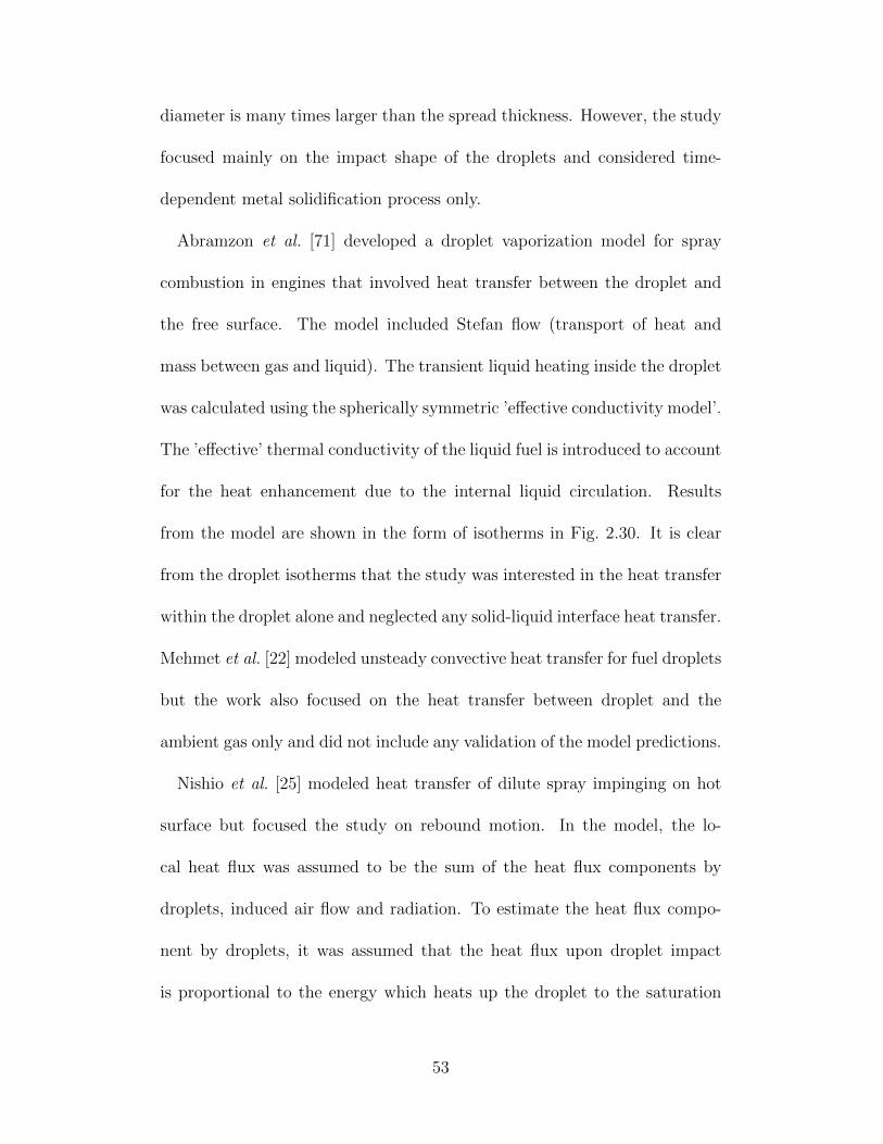
diameter is many times larger than the spread thickness. However, the study

focused mainly on the impact shape of the droplets and considered time-

dependent metal solidification process only.

Abramzon et al. [71] developed a droplet vaporization model for spray

combustion in engines that involved heat transfer between the droplet and

the free surface. The model included Stefan flow (transport of heat and

mass between gas and liquid). The transient liquid heating inside the droplet

was calculated using the spherically symmetric ’effective conductivity model’.

The ’effective’ thermal conductivity of the liquid fuel is introduced to account

for the heat enhancement due to the internal liquid circulation. Results

from the model are shown in the form of isotherms in Fig. 2.30. It is clear

from the droplet isotherms that the study was interested in the heat transfer

within the droplet alone and neglected any solid-liquid interface heat transfer.

Mehmet et al. [22] modeled unsteady convective heat transfer for fuel droplets

but the work also focused on the heat transfer between droplet and the

ambient gas only and did not include any validation of the model predictions.

Nishio et al. [25] modeled heat transfer of dilute spray impinging on hot

surface but focused the study on rebound motion. In the model, the lo-

cal heat flux was assumed to be the sum of the heat flux components by

droplets, induced air flow and radiation. To estimate the heat flux compo-

nent by droplets, it was assumed that the heat flux upon droplet impact

is proportional to the energy which heats up the droplet to the saturation

53

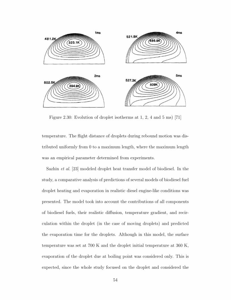
Figure 2.30: Evolution of droplet isotherms at 1, 2, 4 and 5 ms) [71]

temperature. The flight distance of droplets during rebound motion was dis-

tributed uniformly from 0 to a maximum length, where the maximum length

was an empirical parameter determined from experiments.

Sazhin et al. [23] modeled droplet heat transfer model of biodiesel. In the

study, a comparative analysis of predictions of several models of biodiesel fuel

droplet heating and evaporation in realistic diesel engine-like conditions was

presented. The model took into account the contributions of all components

of biodiesel fuels, their realistic diffusion, temperature gradient, and recir-

culation within the droplet (in the case of moving droplets) and predicted

the evaporation time for the droplets. Although in this model, the surface

temperature was set at 700 K and the droplet initial temperature at 360 K,

evaporation of the droplet due at boiling point was considered only. This is

expected, since the whole study focused on the droplet and considered the

54

solid-liquid interface as a fixed temperature boundary only.

Yang et al. [24] developed a 3D modeling of droplet heat transfer to un-

derstand the fundamental nature of the heat transfer phenomenon of a sub-

cooled droplet upon impact with a superheated flat surface. The numerical

technique adopted in their model involved a finite-volume algorithm coupled

with the level-set methods that tracks the deformation of the droplet surface.

The model included film boiling phenomenon and considered vapor film heat

transfer. The temperature profile from the model is shown in Fig. 2.31. The

model predicted the time-dependent variation of the super-heated surface

temperature, but it did not include any heat source term as encountered in

machining and also considered the surface to be isothermal.

Bernardin et al. [26] also studied film boiling heat transfer of droplet

streams but the relied on empirical correlations based on single droplet

stream characteristics and did not include any droplet-surface interaction

2.6 Literature Gap

The atomized spray system has demonstrated that it can improve tool life

compared to flood cooling techniques by reducing the average tool tempera-

ture but the process by which it does is largely unknown. There is a lack of

physics-based understanding of the heat transfer phenomena when the ACF

spray system is used that leads lowering of the cutting temperature and in-

creasing the tool life. A possible way of understanding the mechanism could

55

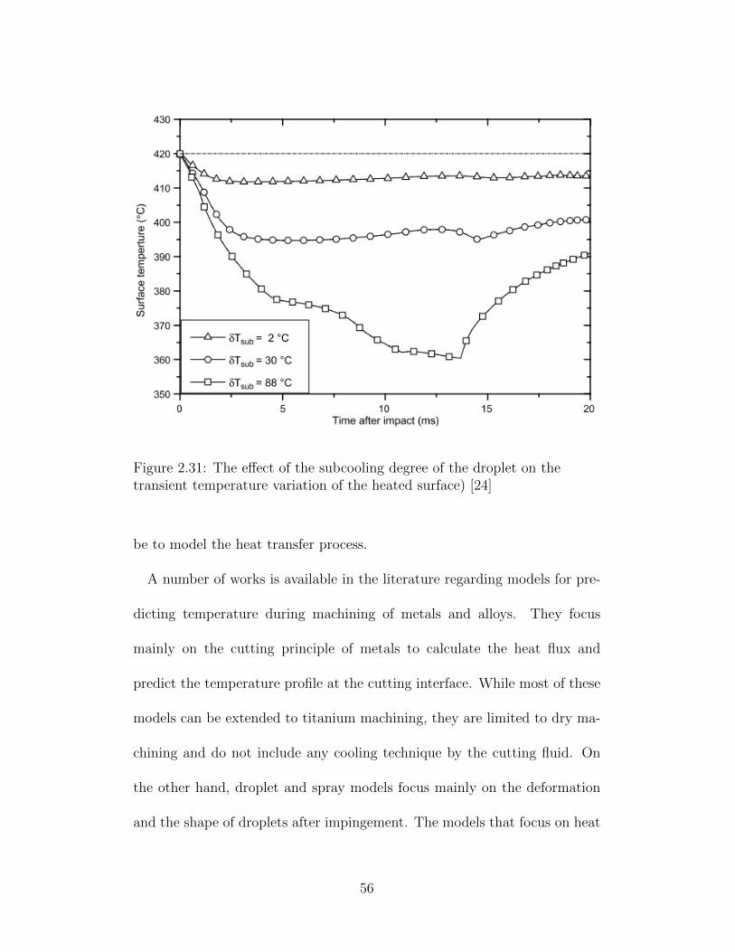
Figure 2.31: The effect of the subcooling degree of the droplet on thetransient temperature variation of the heated surface) [24]

be to model the heat transfer process.

A number of works is available in the literature regarding models for pre-

dicting temperature during machining of metals and alloys. They focus

mainly on the cutting principle of metals to calculate the heat flux and

predict the temperature profile at the cutting interface. While most of these

models can be extended to titanium machining, they are limited to dry ma-

chining and do not include any cooling technique by the cutting fluid. On

the other hand, droplet and spray models focus mainly on the deformation

and the shape of droplets after impingement. The models that focus on heat

56

transfer of droplets mostly deal with splashing and evaporation mechanism

of droplets at much lower temperatures than those faced in machining. Ad-

ditionally, the thermal models concentrate on the variation of temperature

within the droplets, since many of these models have been developed for

spray mechanisms in engines. As a result, the current study needs to be fo-

cused on combining the machining heat generation in the tool with the heat

transfer from the tool with the aid of droplets/spray.

A study of film formation due to ACF spray impingement has also been

made on a cold tool surface. However, the temperature measurements taken

show that a very high average temperature (∼ 600◦C) is reached during

turning of titanium alloys that is likely to initiate boiling heat transfer. Also,

the boiling regime should govern if a film or droplets are formed at the cutting

interface. Therefore, the model to be developed for the problem should

consider the effects of boiling on the ACF spray droplets being impinged

on to the heated surface of the tool. Additionally, the model should be able

to generate a thermal profile for the tool and predict the temperature near

the cutting edge for machining of titanium alloys with ACF spray system.

In the initial studies of the ACF spray system, carbon dioxide seemed to

play an important role in reducing the tool temperature. As a result, a study

on the effect of the gas on the ACF spray cooling mechanism also needs to

be explored.

57

CHAPTER 3

HEAT TRANSFER MODEL OFATOMIZED-BASED CUTTING FLUID(ACF) SYSTEM

Atomized-based cutting fluid (ACF) spray system has been established

as a viable alternative for difficult-to-cut materials such as Ti alloys [7].

Through the use of atomized cutting fluid (ACF) spray system the tool

temperature has been significantly reduced [10]. While it has been estab-

lished that ACF spray system is an efficient technique for cooling and lu-

brication in machining, the studies have been primarily experimental in na-

ture [8, 10, 7, 9]. In order to effectively use the ACF spray system in ma-

chining, it is essential to understand the spray droplet interaction with the

heated tool surface and the mechanism of heat transfer that takes place at

the cutting interface.

3.1 Thermal Model Development

In machining Ti-6Al-4V, the temperature can reach as high as 600◦C

with the use of cutting fluid. As a result, it is highly possible that boiling

heat transfer takes place at the cutting interface. However, boiling involves

different heat transfer regimes including nucleate and film boiling depending

on temperature rise. In order to identify the mechanism that is taking place

58

during machining, a controlled experiment where the WC tool is placed on

a hot plate and the cutting-fluid is sprayed on the rake face of the tool is

carried out. The plate is gradually heated to over 300◦C and the temperature

of the plate/tool is measured with a K-type thermocouple. It is seen that

a film is formed for the first few minutes (See Fig. 3.1(a)). However, with

time, nucleate boiling is seen to occur near the cutting edge (Fig. 3.1(b)) and

after 15 minutes when the temperature is over 300◦C, the droplets impinged

from the ACF spray system are seen to be skittering around indicating that

Leidendfrost point has been reached and the film boiling may be occurring

(Fig. 3.1). Since the maximum temperature reached in this experiment is

much lower than the tool temperature observed during machining Ti-6Al-4V

(300◦C<600◦C), it can be safely assumed that vapor film boiling through the

spreading droplet will dominate during actual machining.

The procedure involved in developing the thermal model that includes

film boiling heat transfer shown in Fig. 3.2. First, the initial temperature of

the tool surface on which the droplet is being impinged is determined from

the heat flux, q′ generated during cutting [72]. The heat flux due to film

boiling is determined next. Since the film boiling heat flux is a function of

heated tool surface temperature and the vapor film thickness, the vapor film

thickness is obtained using the maximum spreading length of the droplet,

which in turn depends on the spreading regime droplet velocity. Finally,

the tool temperature field due to boiling heat transfer that takes place at

59

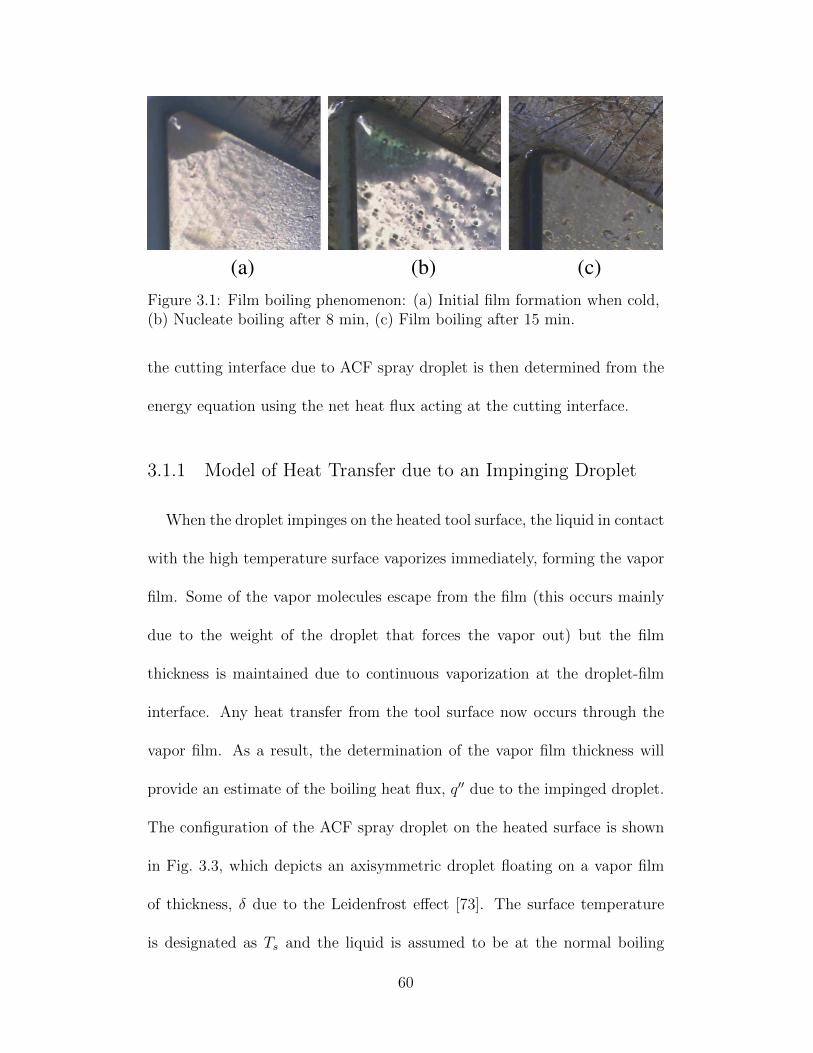
(a) (b) (c)Figure 3.1: Film boiling phenomenon: (a) Initial film formation when cold,(b) Nucleate boiling after 8 min, (c) Film boiling after 15 min.

the cutting interface due to ACF spray droplet is then determined from the

energy equation using the net heat flux acting at the cutting interface.

3.1.1 Model of Heat Transfer due to an Impinging Droplet

When the droplet impinges on the heated tool surface, the liquid in contact

with the high temperature surface vaporizes immediately, forming the vapor

film. Some of the vapor molecules escape from the film (this occurs mainly

due to the weight of the droplet that forces the vapor out) but the film

thickness is maintained due to continuous vaporization at the droplet-film

interface. Any heat transfer from the tool surface now occurs through the

vapor film. As a result, the determination of the vapor film thickness will

provide an estimate of the boiling heat flux, q′′ due to the impinged droplet.

The configuration of the ACF spray droplet on the heated surface is shown

in Fig. 3.3, which depicts an axisymmetric droplet floating on a vapor film

of thickness, δ due to the Leidenfrost effect [73]. The surface temperature

is designated as Ts and the liquid is assumed to be at the normal boiling

60

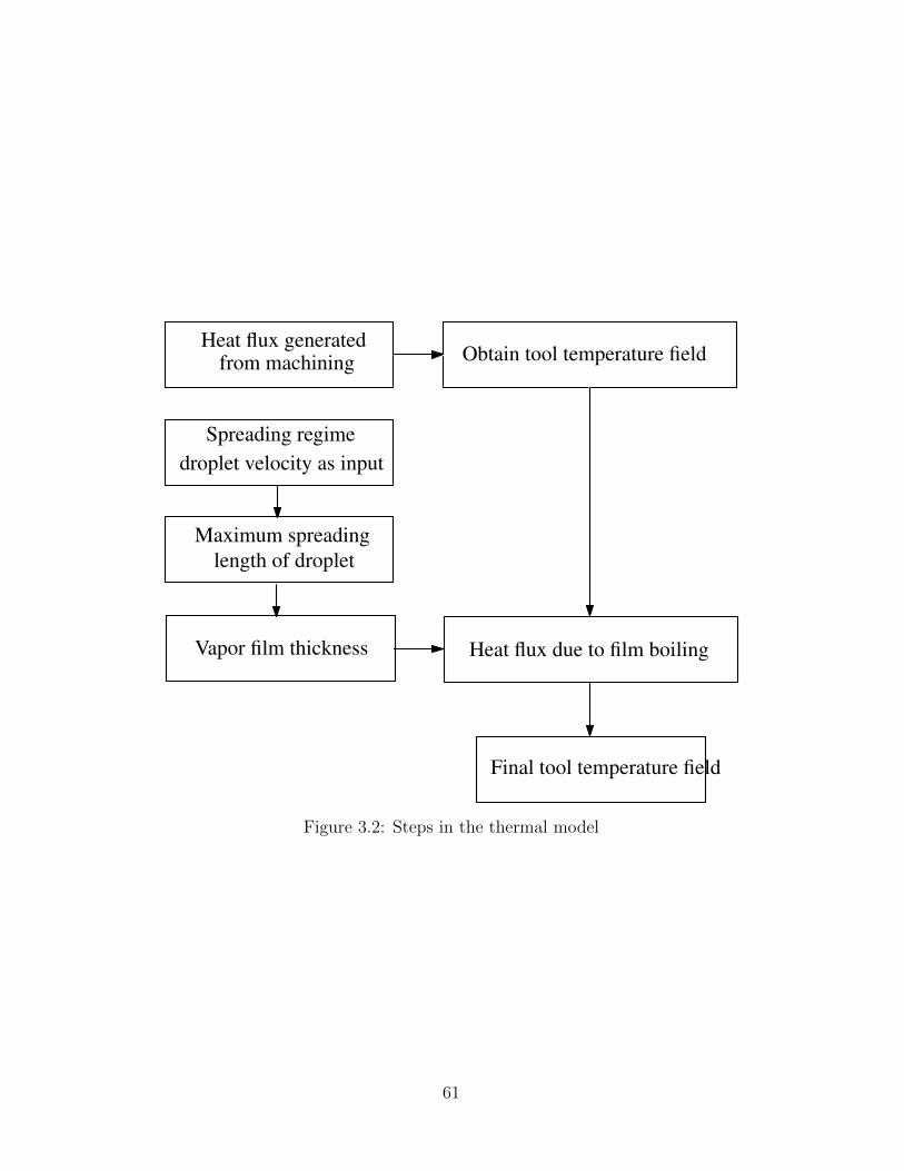
Spreading regime

from machining

Maximum spreading

droplet velocity as input

Heat flux due to film boiling

Heat flux generated

length of droplet

Obtain tool temperature field

Vapor film thickness

Final tool temperature field

Figure 3.2: Steps in the thermal model

61

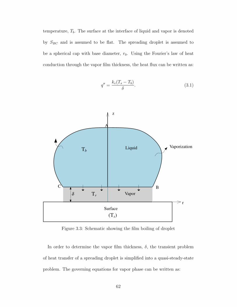
temperature, Tb. The surface at the interface of liquid and vapor is denoted

by SBC and is assumed to be flat. The spreading droplet is assumed to

be a spherical cap with base diameter, r0. Using the Fourier’s law of heat

conduction through the vapor film thickness, the heat flux can be written as:

q′′ =kv(Ts − Tb)

δ. (3.1)

TbLiquid

Tv

Surface

(Ts)

r

z

Vapor

C

A

Bδ

Vaporization

Figure 3.3: Schematic showing the film boiling of droplet

In order to determine the vapor film thickness, δ, the transient problem

of heat transfer of a spreading droplet is simplified into a quasi-steady-state

problem. The governing equations for vapor phase can be written as:

62

Continuity:

ρvv = ρvdδ

dt− ρl

ds

dt, (3.2)

where, v represent axial component of vapor velocity in the film, ρv is the

vapor density, ρl is the liquid density, ds/dt represents the surface (SBC)

recession rate due to evaporation.

Momentum:

µv∂2u

∂z2=∂p

∂r, (3.3)

∂p

∂z= −ρvg, (3.4)

1

r

∂(ru)

∂r+∂v

∂z= 0, (3.5)

where, µv is the vapor viscosity, p is the vapor pressure and u is the radial

velocity. Equations 3.2–3.5 are subject to the following boundary conditions:

u

∣∣∣∣z=0

= v

∣∣∣∣z=0

= 0, and u

∣∣∣∣z=δ

= 0. (no slip condition) (3.6)

Since heat flows from the tool surface to the vapor film, any heat transfer

within the vapor film along the radial direction is assumed to be negligible.

As a result, the energy equation for the vapor film thickness can be written

as,

Energy:

kv∂2T

∂z2= 0, (3.7)

63

where, kv is the vapor thermal conductivity. Equation 3.7 is solved using the

following boundary conditions:

T

∣∣∣∣z=0

= Ts, T

∣∣∣∣z=δ

= Tb, and (3.8)

ρlLvds

dt= −kv

∂T

∂z

∣∣∣∣z=δ

. (3.9)

It is assumed that the liquid is at a constant temeprature equal to the boiling

temperature. ρl is the liquid density, Lv is the latent heat of vaporization.

Equation 3.9 represents the Stefan’s condition that describes evaporation due

to the heat flux from liquid to vapor.

The steady-state vapor film thickness, δ can be obtained by solving Eq 3.7–

3.9, and is given as:

δ =kvρlLv

(Tb − Ts)ds/dt

. (3.10)

The recession rate, ds/dt can be determined by studying the force balance

of the droplet weight and force caused by the vapor pressure. The force

balance is expressed as:

ρlV (t)g = 2π

∫ r0

0

rpdr, (3.11)

where, V (t) represents the liquid volume. The volume, V (t) can be deter-

mined by subtracting the volume of the evaporated droplets from the initial

64

droplet volume, V0 as,

V (t) = V0 −∫ t

0

(SBC

ds

dt+ SBAC

df

dt

), (3.12)

where, df/dt represents the evaporation rate over the surface SBAC . Since

(SBAC) is very small compared to that of vaporization at the liquid-vapor

interface it can be ignored.

The vapor pressure, p can be determined by first solving the momen-

tum Eq. 3.3–3.5 for the axial and radial vapor velocities and then using

the continuity Eq. 3.2 along with the boundary conditions given in Eq. 3.6

and applying the pressure boundary as the pressure boundary condition

(p = 0, r = Dmax/2). The velocities and pressure are obtained as:

u =1

2µv

(∂p

∂r

)[z(z − δ)]. (3.13)

v = − 1

12µvr

∂

∂r

(r∂p

∂r

)· z2(2z − 3δ). (3.14)

p =3µvδ3

(dδ

dt− ρlρv

ds

dt

)(r2 − r20

). (3.15)

Substituting the expression of pressure, p from Eq. 3.15 in the force balance

Eq. 3.11 yields:

ρlV (t)g =3πµvr

40

2δ3

(dδ

dt− ρlρv

ds

dt

). (3.16)

For steady-state condition, dδ/dt is zero. The steady-state vapor film thick-

ness can now be obtained from Eq. 3.10 by substituting the expression for

65

ds/dt from Eq. 3.16 and is given as:

δ =

(9µvkvr0(Ts − Tb)

8ρvρlgLv

)1/4

. (3.17)

The evaluation of base diameter of the droplet, r0 in Eq. 3.17 is discussed

in the next section. The film thickness, δ for Eq. 3.17 can be substituted in

Eq 3.1 to obtain the heat flux, q′′.

Finally, knowing the net heat flux acting at the cutting interface as, q′−q′′,

the boundary condition at the cutting interface can be given as:

q′ − q′′ = kc∂T

∂z

∣∣∣∣z=0

, (3.18)

where kc is the thermal conductivity of the tool material. Using this bound-

ary, the temperature field of the whole tool can be obtained using the energy

equation for the tool:

kc(∂2T

∂x2+∂2T

∂y2+∂2T

∂z2) = 0, (3.19)

where dx, dy and dz represent the differential dimensions of the tool.

Determination of the Base Diameter of the Droplet, r0:

To determine r0 of the impinging droplet, energy balance of the droplet

just before and after impingement and at its maximum spreading condition

66

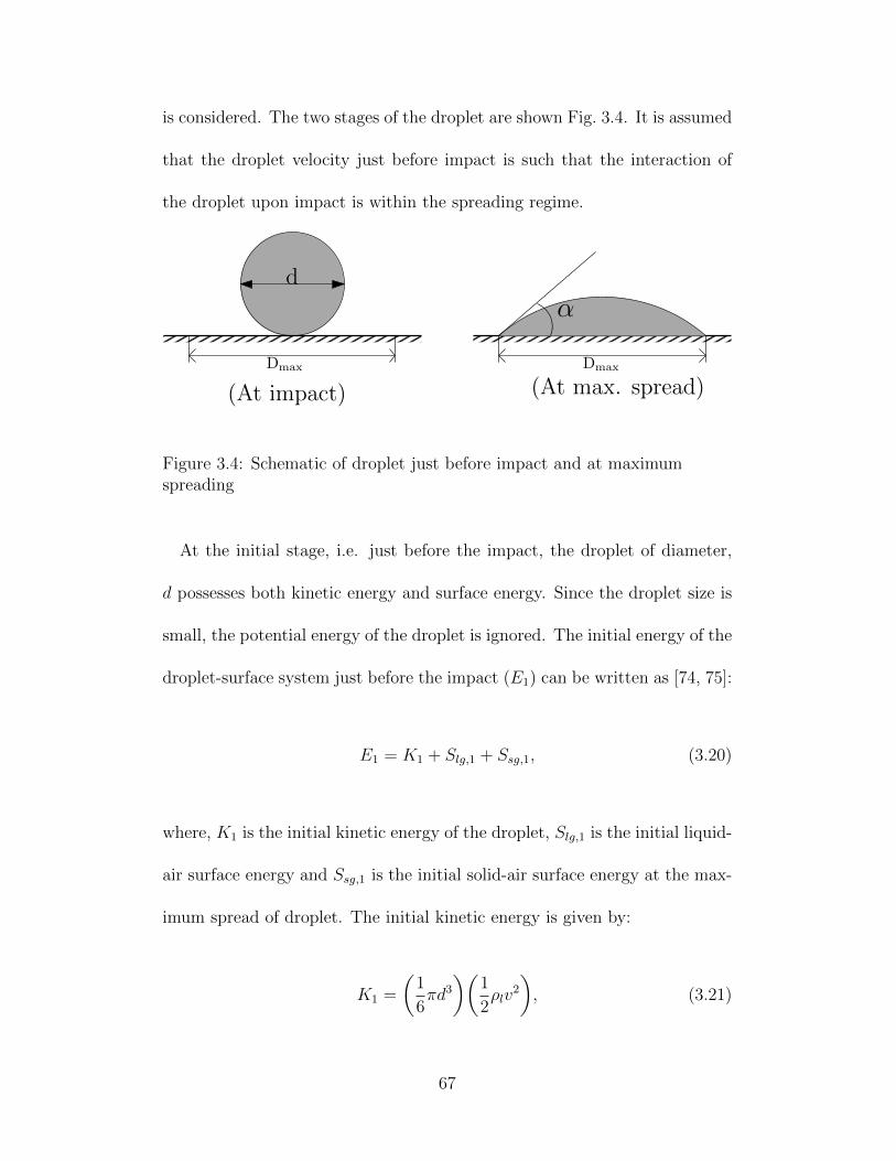
is considered. The two stages of the droplet are shown Fig. 3.4. It is assumed

that the droplet velocity just before impact is such that the interaction of

the droplet upon impact is within the spreading regime.

α

Dmax Dmax

d

(At impact) (At max. spread)

Figure 3.4: Schematic of droplet just before impact and at maximumspreading

At the initial stage, i.e. just before the impact, the droplet of diameter,

d possesses both kinetic energy and surface energy. Since the droplet size is

small, the potential energy of the droplet is ignored. The initial energy of the

droplet-surface system just before the impact (E1) can be written as [74, 75]:

E1 = K1 + Slg,1 + Ssg,1, (3.20)

where, K1 is the initial kinetic energy of the droplet, Slg,1 is the initial liquid-

air surface energy and Ssg,1 is the initial solid-air surface energy at the max-

imum spread of droplet. The initial kinetic energy is given by:

K1 =

(1

6πd3)(

1

2ρlv

2

), (3.21)

67

where ρ and v are density and velocity of the droplet, respectively. The

initial surface energies are given by:

Slg,1 = πd2σlg, (3.22)

Ssg,1 =1

4πD2

maxσsg, (3.23)

where, σlg and σsg represent the liquid-air surface tension and solid-air surface

tension, respectively; and Dmax is the maximum spreading length of the

droplet and v is the velocity of the droplet.

The final energy of the droplet-surface system at maximum spreading

length can be written as

E2 = K2 + Slg,2 + Ssl,2, (3.24)

where, K2 is the final kinetic energy of the droplet, Slg,2 is the final liquid-air

surface energy and Ssl,2 is the final interfacial kinetic energy between the

liquid and the surface. Since, the droplet comes to a rest at its maximum

spreading length, K2 = 0. Assuming the droplet takes the shape of a spheri-

cal cap and the volume of the fluid is constant, the liquid-air surface energy

can be written in terms of the contact angle (α) at maximum spreading

length:

Slg,2 =1

2π(1− cosα)

(4

2− 3 cosα + cos3 α

)2/3

d2σlg. (3.25)

68

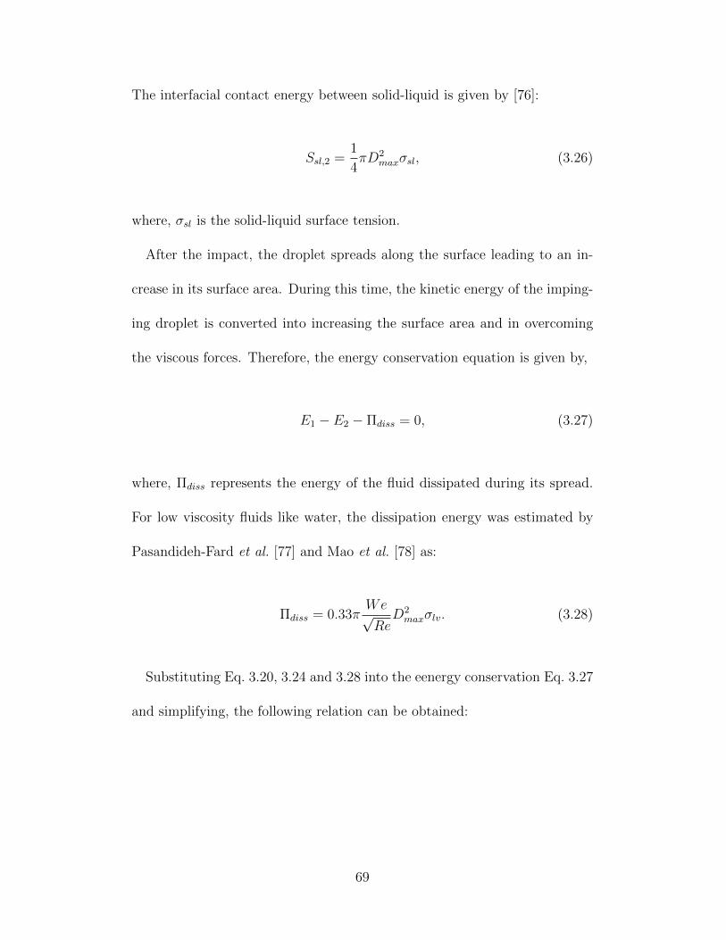
The interfacial contact energy between solid-liquid is given by [76]:

Ssl,2 =1

4πD2

maxσsl, (3.26)

where, σsl is the solid-liquid surface tension.

After the impact, the droplet spreads along the surface leading to an in-

crease in its surface area. During this time, the kinetic energy of the imping-

ing droplet is converted into increasing the surface area and in overcoming

the viscous forces. Therefore, the energy conservation equation is given by,

E1 − E2 − Πdiss = 0, (3.27)

where, Πdiss represents the energy of the fluid dissipated during its spread.

For low viscosity fluids like water, the dissipation energy was estimated by

Pasandideh-Fard et al. [77] and Mao et al. [78] as:

Πdiss = 0.33πWe√Re

D2maxσlv. (3.28)

Substituting Eq. 3.20, 3.24 and 3.28 into the eenergy conservation Eq. 3.27

and simplifying, the following relation can be obtained:

69

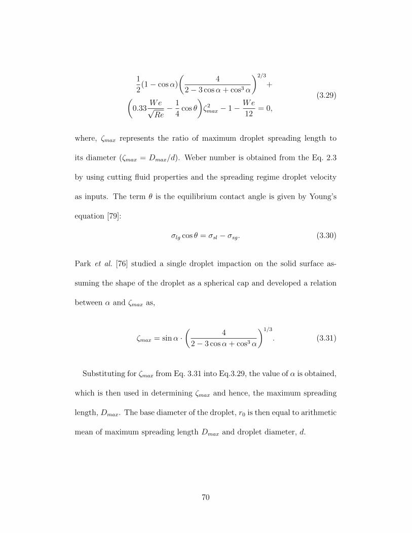
1

2(1− cosα)

(4

2− 3 cosα + cos3 α

)2/3

+(0.33

We√Re− 1

4cos θ

)ζ2max − 1− We

12= 0,

(3.29)

where, ζmax represents the ratio of maximum droplet spreading length to

its diameter (ζmax = Dmax/d). Weber number is obtained from the Eq. 2.3

by using cutting fluid properties and the spreading regime droplet velocity

as inputs. The term θ is the equilibrium contact angle is given by Young’s

equation [79]:

σlg cos θ = σsl − σsg. (3.30)

Park et al. [76] studied a single droplet impaction on the solid surface as-

suming the shape of the droplet as a spherical cap and developed a relation

between α and ζmax as,

ζmax = sinα ·(

4

2− 3 cosα + cos3 α

)1/3

. (3.31)

Substituting for ζmax from Eq. 3.31 into Eq.3.29, the value of α is obtained,

which is then used in determining ζmax and hence, the maximum spreading

length, Dmax. The base diameter of the droplet, r0 is then equal to arithmetic

mean of maximum spreading length Dmax and droplet diameter, d.

70

3.2 Chapter Summary

In this chapter, the thermal model developed for the ACF spray system to

predict the temperature of the cutting tool is described. The model considers

film boiling as the major heat transfer phenomenon. Film boiling is caused

by the high temperature involved in turning of Ti-6Al-4V alloy. Due to

this high temperature, the cutting-fluid spray droplets from the ACF spray

system form a thin vapor film between themselves and the heated surface due

to the rapid vaporization of the liquid when it comes into contact with the

surface. In the model, heat transfer through this film by conduction is carried

out. Additionally, the model takes into account the temperature variation

on the tool surface and develops a film thickness expression as a function of

tool surface temperature. The model also considers the deformation of the

droplet by taking the maximum spread diameter of the droplet to calculate

the film thickness. By obtaining the film thickness, the boiling heat flux and

hence, the temperature profile of the tool can be determined. The predicted

results and the validation are discussed in Chapter 5.

71

CHAPTER 4

SPRAY GENERATION MODEL

Since the degree of cooling due to boiling heat transfer that takes place

at the cutting interface largely depends on spray characteristics including

droplet velocity, a spray model is developed to predict droplet velocity profiles

along the spray distance for a given droplet diameter and gas pressure, and

establish the spray distance range where the droplets are within the spreading

regime needed for ACF spray cooling. The approach used in modeling of the

ACF spray is described in this section.

4.1 Spray Model

The model developed to study the spray behavior of the ACF spray system

involves two stages: the gas model and the droplet model. The gas model

is used for solving the steady-state velocity field of the gas emerging out of

the nozzle at a certain high pressure, assuming the flow to be compressible.

This is followed by solving for the droplet velocity profiles in the presence of

the gas field. The droplets are introduced into the flow field from a droplet

generator (source). Droplet velocities are tracked at different positions as

the droplets traverse through the gas flow field.

72

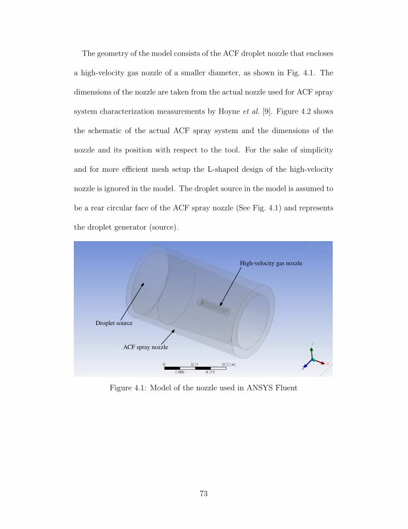
The geometry of the model consists of the ACF droplet nozzle that encloses

a high-velocity gas nozzle of a smaller diameter, as shown in Fig. 4.1. The

dimensions of the nozzle are taken from the actual nozzle used for ACF spray

system characterization measurements by Hoyne et al. [9]. Figure 4.2 shows

the schematic of the actual ACF spray system and the dimensions of the

nozzle and its position with respect to the tool. For the sake of simplicity

and for more efficient mesh setup the L-shaped design of the high-velocity

nozzle is ignored in the model. The droplet source in the model is assumed to

be a rear circular face of the ACF spray nozzle (See Fig. 4.1) and represents

the droplet generator (source).

Droplet source

High-velocity gas nozzle

ACF spray nozzle

Figure 4.1: Model of the nozzle used in ANSYS Fluent

73

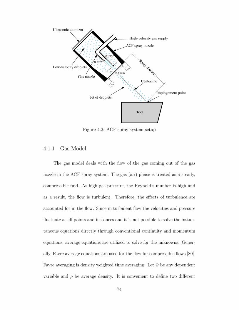
Ultrasonic atomizer

Tool

Jet of droplets

ACF spray nozzle

Gas nozzle

Low-velocity droplets

High-velocity gas supply

0.375o

0.375o

2o

2o

1.6 mm 18.8 mm

Spray distance

Impingement point

Centerline

Figure 4.2: ACF spray system setup

4.1.1 Gas Model

The gas model deals with the flow of the gas coming out of the gas

nozzle in the ACF spray system. The gas (air) phase is treated as a steady,

compressible fuid. At high gas pressure, the Reynold’s number is high and

as a result, the flow is turbulent. Therefore, the effects of turbulence are

accounted for in the flow. Since in turbulent flow the velocities and pressure

fluctuate at all points and instances and it is not possible to solve the instan-

taneous equations directly through conventional continuity and momentum

equations, average equations are utilized to solve for the unknowns. Gener-

ally, Favre average equations are used for the flow for compressible flows [80].

Favre averaging is density weighted time averaging. Let Φ be any dependent

variable and ρ be average density. It is convenient to define two different

74

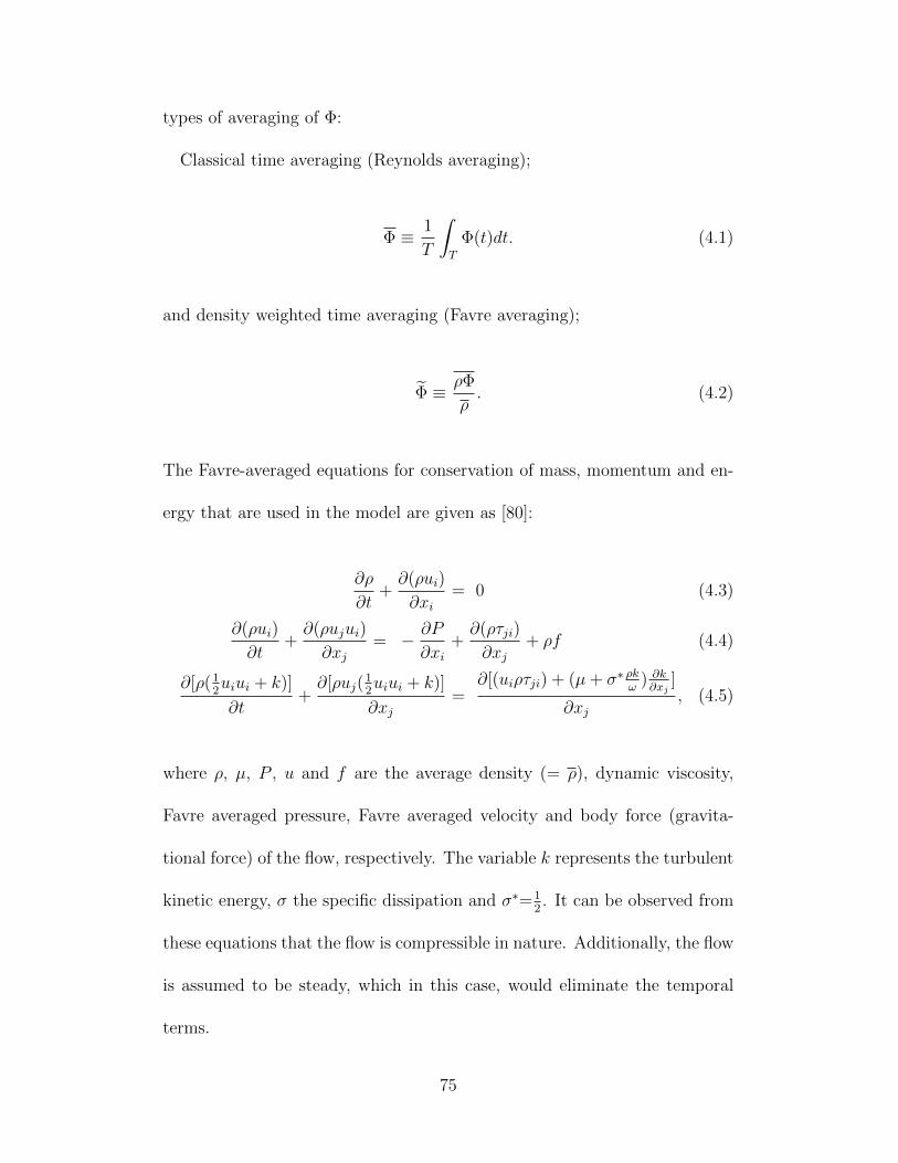
types of averaging of Φ:

Classical time averaging (Reynolds averaging);

Φ ≡ 1

T

∫T

Φ(t)dt. (4.1)

and density weighted time averaging (Favre averaging);

Φ ≡ ρΦ

ρ. (4.2)

The Favre-averaged equations for conservation of mass, momentum and en-

ergy that are used in the model are given as [80]:

∂ρ

∂t+∂(ρui)

∂xi= 0 (4.3)

∂(ρui)

∂t+∂(ρujui)

∂xj= − ∂P

∂xi+∂(ρτji)

∂xj+ ρf (4.4)

∂[ρ(12uiui + k)]

∂t+∂[ρuj(

12uiui + k)]

∂xj=

∂[(uiρτji) + (µ+ σ∗ ρkω

) ∂k∂xj

]

∂xj, (4.5)

where ρ, µ, P , u and f are the average density (= ρ), dynamic viscosity,

Favre averaged pressure, Favre averaged velocity and body force (gravita-

tional force) of the flow, respectively. The variable k represents the turbulent

kinetic energy, σ the specific dissipation and σ∗=12. It can be observed from

these equations that the flow is compressible in nature. Additionally, the flow

is assumed to be steady, which in this case, would eliminate the temporal

terms.

75

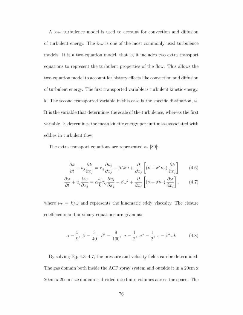
A k-ω turbulence model is used to account for convection and diffusion

of turbulent energy. The k-ω is one of the most commonly used turbulence

models. It is a two-equation model, that is, it includes two extra transport

equations to represent the turbulent properties of the flow. This allows the

two-equation model to account for history effects like convection and diffusion

of turbulent energy. The first transported variable is turbulent kinetic energy,

k. The second transported variable in this case is the specific dissipation, ω.

It is the variable that determines the scale of the turbulence, whereas the first

variable, k, determines the mean kinetic energy per unit mass associated with

eddies in turbulent flow.

The extra transport equations are represented as [80]:

∂k

∂t+ uj

∂k

∂xj= τij

∂ui∂xj− β∗kω +

∂

∂xj

[(ν + σ∗νT )

∂k

∂xj

](4.6)

∂ω

∂t+ uj

∂ω

∂xj= α

ω

kτij∂ui∂xj− βω2 +

∂

∂xj

[(ν + σνT )

∂ω

∂xj

], (4.7)

where νT = k/ω and represents the kinematic eddy viscosity. The closure

coefficients and auxiliary equations are given as:

α =5

9, β =

3

40, β∗ =

9

100, σ =

1

2, σ∗ =

1

2, ε = β∗ωk (4.8)

By solving Eq. 4.3–4.7, the pressure and velocity fields can be determined.

The gas domain both inside the ACF spray system and outside it in a 20cm x

20cm x 20cm size domain is divided into finite volumes across the space. The

76

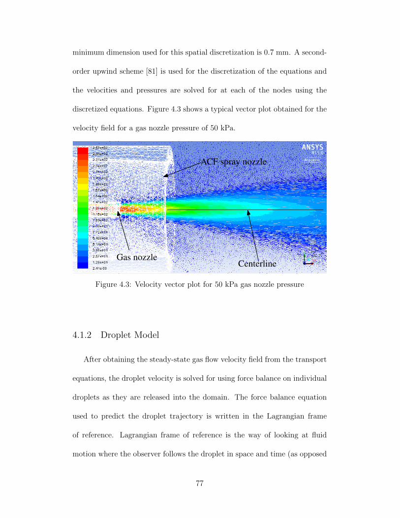
minimum dimension used for this spatial discretization is 0.7 mm. A second-

order upwind scheme [81] is used for the discretization of the equations and

the velocities and pressures are solved for at each of the nodes using the

discretized equations. Figure 4.3 shows a typical vector plot obtained for the

velocity field for a gas nozzle pressure of 50 kPa.

CenterlineGas nozzle

ACF spray nozzle

Figure 4.3: Velocity vector plot for 50 kPa gas nozzle pressure

4.1.2 Droplet Model

After obtaining the steady-state gas flow velocity field from the transport

equations, the droplet velocity is solved for using force balance on individual

droplets as they are released into the domain. The force balance equation

used to predict the droplet trajectory is written in the Lagrangian frame

of reference. Lagrangian frame of reference is the way of looking at fluid

motion where the observer follows the droplet in space and time (as opposed

77

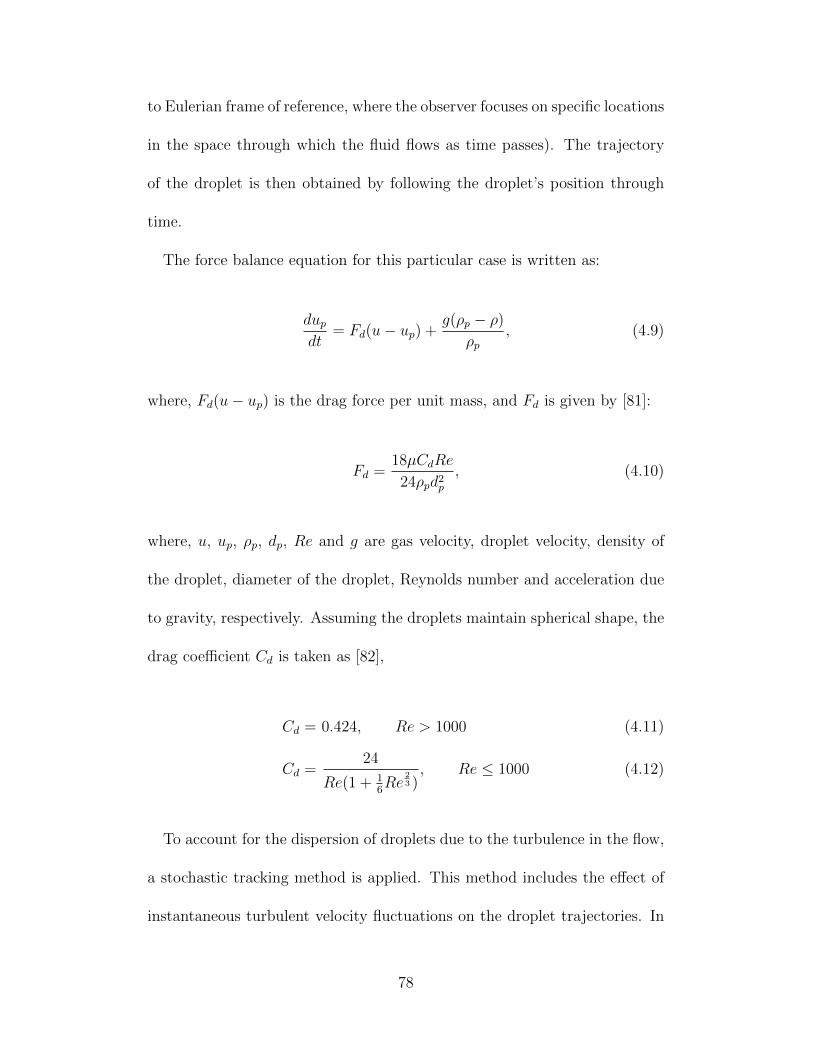
to Eulerian frame of reference, where the observer focuses on specific locations

in the space through which the fluid flows as time passes). The trajectory

of the droplet is then obtained by following the droplet’s position through

time.

The force balance equation for this particular case is written as:

dupdt

= Fd(u− up) +g(ρp − ρ)

ρp, (4.9)

where, Fd(u− up) is the drag force per unit mass, and Fd is given by [81]:

Fd =18µCdRe

24ρpd2p, (4.10)

where, u, up, ρp, dp, Re and g are gas velocity, droplet velocity, density of

the droplet, diameter of the droplet, Reynolds number and acceleration due

to gravity, respectively. Assuming the droplets maintain spherical shape, the

drag coefficient Cd is taken as [82],

Cd = 0.424, Re > 1000 (4.11)

Cd =24

Re(1 + 16Re

23 ), Re ≤ 1000 (4.12)

To account for the dispersion of droplets due to the turbulence in the flow,

a stochastic tracking method is applied. This method includes the effect of

instantaneous turbulent velocity fluctuations on the droplet trajectories. In

78

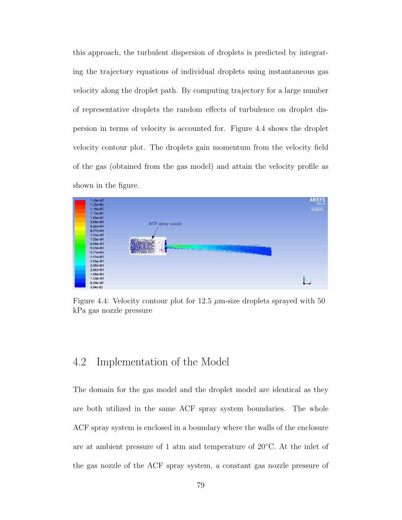
this approach, the turbulent dispersion of droplets is predicted by integrat-

ing the trajectory equations of individual droplets using instantaneous gas

velocity along the droplet path. By computing trajectory for a large number

of representative droplets the random effects of turbulence on droplet dis-

persion in terms of velocity is accounted for. Figure 4.4 shows the droplet

velocity contour plot. The droplets gain momentum from the velocity field

of the gas (obtained from the gas model) and attain the velocity profile as

shown in the figure.

ACF spray nozzle

Figure 4.4: Velocity contour plot for 12.5 µm-size droplets sprayed with 50kPa gas nozzle pressure

4.2 Implementation of the Model

The domain for the gas model and the droplet model are identical as they

are both utilized in the same ACF spray system boundaries. The whole

ACF spray system is enclosed in a boundary where the walls of the enclosure

are at ambient pressure of 1 atm and temperature of 20◦C. At the inlet of

the gas nozzle of the ACF spray system, a constant gas nozzle pressure of

79

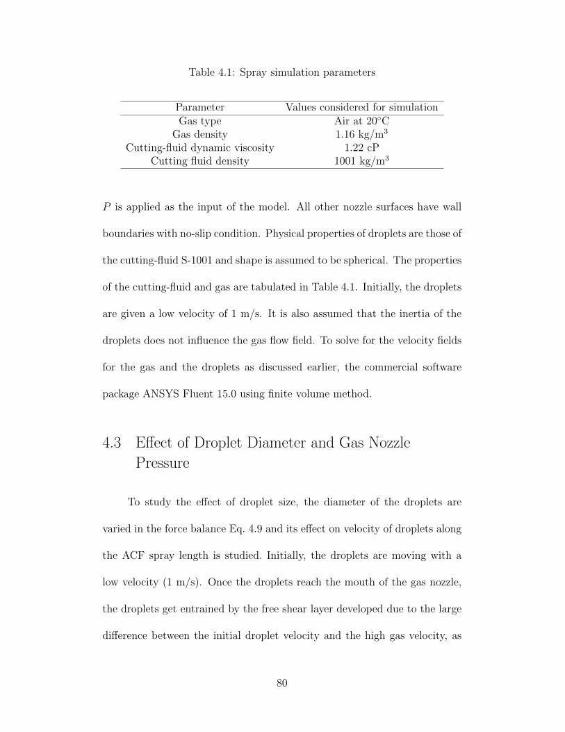
Table 4.1: Spray simulation parameters

Parameter Values considered for simulationGas type Air at 20◦C

Gas density 1.16 kg/m3

Cutting-fluid dynamic viscosity 1.22 cPCutting fluid density 1001 kg/m3

P is applied as the input of the model. All other nozzle surfaces have wall

boundaries with no-slip condition. Physical properties of droplets are those of

the cutting-fluid S-1001 and shape is assumed to be spherical. The properties

of the cutting-fluid and gas are tabulated in Table 4.1. Initially, the droplets

are given a low velocity of 1 m/s. It is also assumed that the inertia of the

droplets does not influence the gas flow field. To solve for the velocity fields

for the gas and the droplets as discussed earlier, the commercial software

package ANSYS Fluent 15.0 using finite volume method.

4.3 Effect of Droplet Diameter and Gas Nozzle

Pressure

To study the effect of droplet size, the diameter of the droplets are

varied in the force balance Eq. 4.9 and its effect on velocity of droplets along

the ACF spray length is studied. Initially, the droplets are moving with a

low velocity (1 m/s). Once the droplets reach the mouth of the gas nozzle,

the droplets get entrained by the free shear layer developed due to the large

difference between the initial droplet velocity and the high gas velocity, as

80

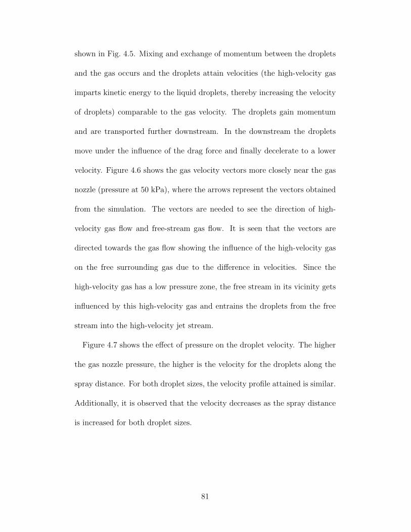
shown in Fig. 4.5. Mixing and exchange of momentum between the droplets

and the gas occurs and the droplets attain velocities (the high-velocity gas

imparts kinetic energy to the liquid droplets, thereby increasing the velocity

of droplets) comparable to the gas velocity. The droplets gain momentum

and are transported further downstream. In the downstream the droplets

move under the influence of the drag force and finally decelerate to a lower

velocity. Figure 4.6 shows the gas velocity vectors more closely near the gas

nozzle (pressure at 50 kPa), where the arrows represent the vectors obtained

from the simulation. The vectors are needed to see the direction of high-

velocity gas flow and free-stream gas flow. It is seen that the vectors are

directed towards the gas flow showing the influence of the high-velocity gas

on the free surrounding gas due to the difference in velocities. Since the

high-velocity gas has a low pressure zone, the free stream in its vicinity gets

influenced by this high-velocity gas and entrains the droplets from the free

stream into the high-velocity jet stream.

Figure 4.7 shows the effect of pressure on the droplet velocity. The higher

the gas nozzle pressure, the higher is the velocity for the droplets along the

spray distance. For both droplet sizes, the velocity profile attained is similar.

Additionally, it is observed that the velocity decreases as the spray distance

is increased for both droplet sizes.

81

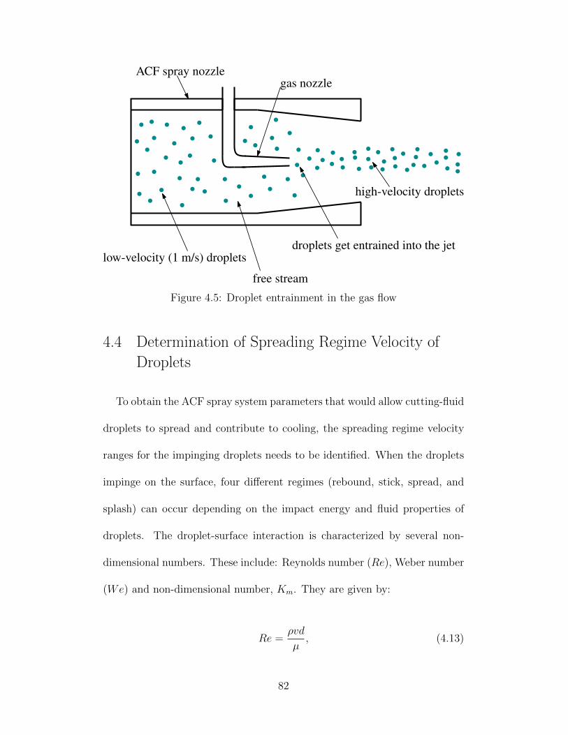
low-velocity (1 m/s) droplets

gas nozzleACF spray nozzle

droplets get entrained into the jet

high-velocity droplets

free stream

Figure 4.5: Droplet entrainment in the gas flow

4.4 Determination of Spreading Regime Velocity of

Droplets

To obtain the ACF spray system parameters that would allow cutting-fluid

droplets to spread and contribute to cooling, the spreading regime velocity

ranges for the impinging droplets needs to be identified. When the droplets

impinge on the surface, four different regimes (rebound, stick, spread, and

splash) can occur depending on the impact energy and fluid properties of

droplets. The droplet-surface interaction is characterized by several non-

dimensional numbers. These include: Reynolds number (Re), Weber number

(We) and non-dimensional number, Km. They are given by:

Re =ρvd

µ, (4.13)

82

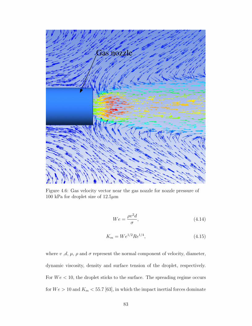
Gas nozzle

Figure 4.6: Gas velocity vector near the gas nozzle for nozzle pressure of100 kPa for droplet size of 12.5µm

We =ρv2d

σ, (4.14)

Km = We1/2Re1/4, (4.15)

where v ,d, µ, ρ and σ represent the normal component of velocity, diameter,

dynamic viscosity, density and surface tension of the droplet, respectively.

For We < 10, the droplet sticks to the surface. The spreading regime occurs

for We > 10 and Km < 55.7 [63], in which the impact inertial forces dominate

83

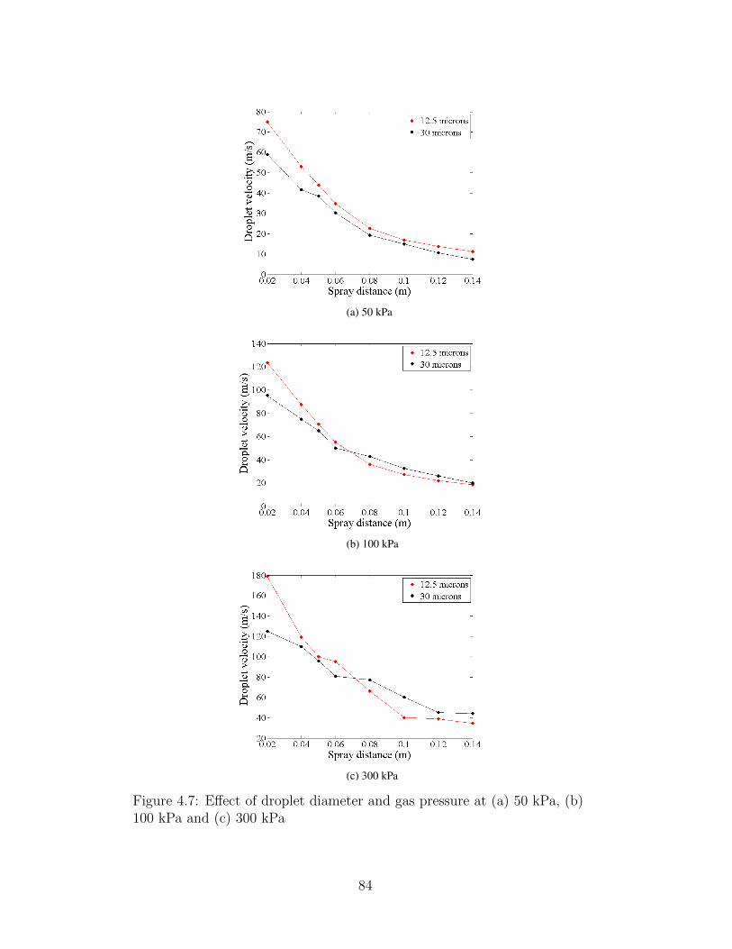
(a) 50 kPa

(b) 100 kPa

(c) 300 kPa

Figure 4.7: Effect of droplet diameter and gas pressure at (a) 50 kPa, (b)100 kPa and (c) 300 kPa

84

and cause spreading of the droplet. For values of Km > 55.7, the impact

inertial forces are so high that splashing occurs and the droplet breaks up

into tiny droplets. Splashing is undesirable in machining as it would lead to

reduction in air quality. Therefore, the spray parameters and fluid properties

need to be selected appropriately to be able to achieve the spreading regime

that will allow the cutting fluid to enter the cutting interface.

The Weber number and Km determine the velocity range that will allow

the droplet to spread on the surface. The variation of We and Km with

droplet’s normal velocity at different droplet diameters is shown in Figs. 4.8

and 4.9, respectively. In the figures, the threshold values of spreading regime

are indicated by horizontal lines for We = 10 and Km = 57.7. For droplet

size of 12.5 µm the droplet velocity between 6 m/s to 40 m/s can ensure

the spreading regime. For 30µm droplet size, the droplet velocity range is

from 4.2 m/s to 24 m/s. Similarly, for droplet size of 80 µm the range is

from 3 m/s to 14 m/s. It is observed that the range of droplet velocities

that correspond to the spreading regime is very narrow for the 80 µm sized

droplet. This shows that droplet diameter sizes from 12.5 to 30 µm could be

used to utilize their wider ranges of spreading regime velocities, with smaller

droplet size providing a greater range of velocities for the spreading regime.

For 12.5µm droplet to be within the spreading regime, the spray distance

has to be set at a minimum of 55 mm at 50 kPa (See Fig. 4.7). Similarly, for

the gas pressures of 100 kPa and 300 kPa, the spray distance is required to

85

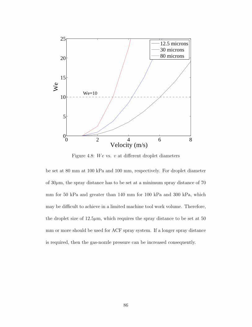
0 2 4 6 80

5

10

15

20

25

Velocity (m/s)

We

12.5 microns30 microns80 microns

We=10

Figure 4.8: We vs. v at different droplet diameters

be set at 80 mm at 100 kPa and 100 mm, respectively. For droplet diameter

of 30µm, the spray distance has to be set at a minimum spray distance of 70

mm for 50 kPa and greater than 140 mm for 100 kPa and 300 kPa, which

may be difficult to achieve in a limited machine tool work volume. Therefore,

the droplet size of 12.5µm, which requires the spray distance to be set at 50

mm or more should be used for ACF spray system. If a longer spray distance

is required, then the gas-nozzle pressure can be increased consequently.

86

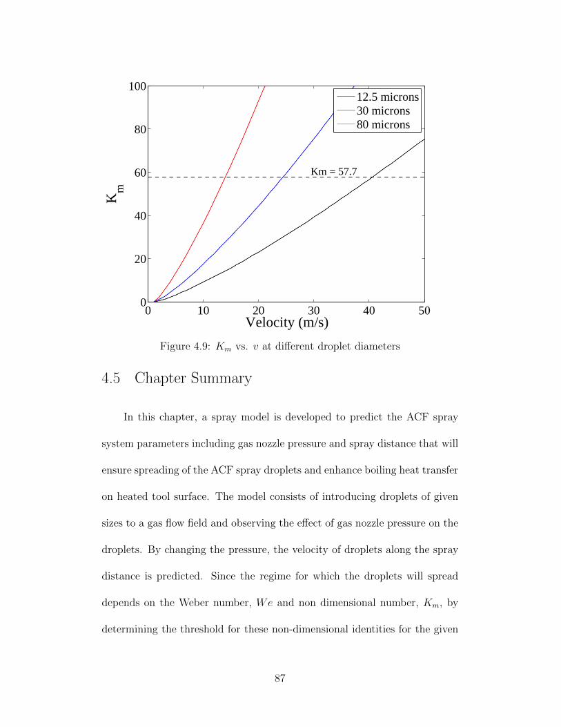
0 10 20 30 40 500

20

40

60

80

100

Velocity (m/s)

Km

12.5 microns30 microns80 microns

Km = 57.7

Figure 4.9: Km vs. v at different droplet diameters

4.5 Chapter Summary

In this chapter, a spray model is developed to predict the ACF spray

system parameters including gas nozzle pressure and spray distance that will

ensure spreading of the ACF spray droplets and enhance boiling heat transfer

on heated tool surface. The model consists of introducing droplets of given

sizes to a gas flow field and observing the effect of gas nozzle pressure on the

droplets. By changing the pressure, the velocity of droplets along the spray

distance is predicted. Since the regime for which the droplets will spread

depends on the Weber number, We and non dimensional number, Km, by

determining the threshold for these non-dimensional identities for the given

87

fluid, the range of spreading velocities are found out. By comparing them

with the model’s droplet velocity profile, the range of distance along which

the droplets will move with spreading regime velocity at different pressure

values is identified.

It is found from the simulation that for 12.5 µm droplet to be within the

spreading regime, the spray distance has to be set at a minimum of 55 mm

at 50 kPa, 80 mm at 100 kPa and 100 mm at 300 kPa. For 30µm droplet

size, the spray distance has to be set at a minimum of 70 mm for 50 kPa and

greater than 140 mm for 100 kPa and 300 kPa, respectively. Accordingly,

the design for an ACF spray system can be made depending on other factors,

such as machine tool work volume available and gas pressure requirements.

88

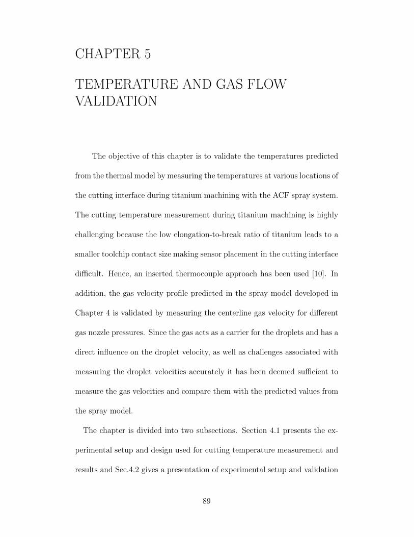
CHAPTER 5

TEMPERATURE AND GAS FLOWVALIDATION

The objective of this chapter is to validate the temperatures predicted

from the thermal model by measuring the temperatures at various locations of

the cutting interface during titanium machining with the ACF spray system.

The cutting temperature measurement during titanium machining is highly

challenging because the low elongation-to-break ratio of titanium leads to a

smaller toolchip contact size making sensor placement in the cutting interface

difficult. Hence, an inserted thermocouple approach has been used [10]. In

addition, the gas velocity profile predicted in the spray model developed in

Chapter 4 is validated by measuring the centerline gas velocity for different

gas nozzle pressures. Since the gas acts as a carrier for the droplets and has a

direct influence on the droplet velocity, as well as challenges associated with

measuring the droplet velocities accurately it has been deemed sufficient to

measure the gas velocities and compare them with the predicted values from

the spray model.

The chapter is divided into two subsections. Section 4.1 presents the ex-

perimental setup and design used for cutting temperature measurement and

results and Sec.4.2 gives a presentation of experimental setup and validation

89

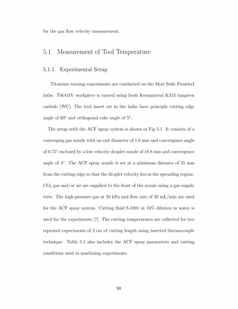
for the gas flow velocity measurement.

5.1 Measurement of Tool Temperature

5.1.1 Experimental Setup

Titanium turning experiments are conducted on the Mori Seiki FrontierI

lathe. Ti6Al4V workpiece is turned using fresh Kennametal K313 tungsten

carbide (WC). The tool insert set in the lathe have principle cutting edge

angle of 60o and orthogonal rake angle of 5o.

The setup with the ACF spray system is shown in Fig 5.1. It consists of a

converging gas nozzle with an exit diameter of 1.6 mm and convergence angle

of 0.75◦ enclosed by a low-velocity droplet nozzle of 18.8 mm and convergence

angle of 4◦. The ACF spray nozzle is set at a minimum distance of 55 mm

from the cutting edge so that the droplet velocity lies in the spreading regime.

CO2 gas and/or air are supplied to the front of the nozzle using a gas supply

tube. The high-pressure gas at 50 kPa and flow rate of 20 mL/min are used

for the ACF spray system. Cutting fluid S-1001 at 10% dilution in water is

used for the experiments [7]. The cutting temperatures are collected for two

repeated experiments of 2 cm of cutting length using inserted thermocouple

technique. Table 5.1 also includes the ACF spray parameters and cutting

conditions used in machining experiments.

90

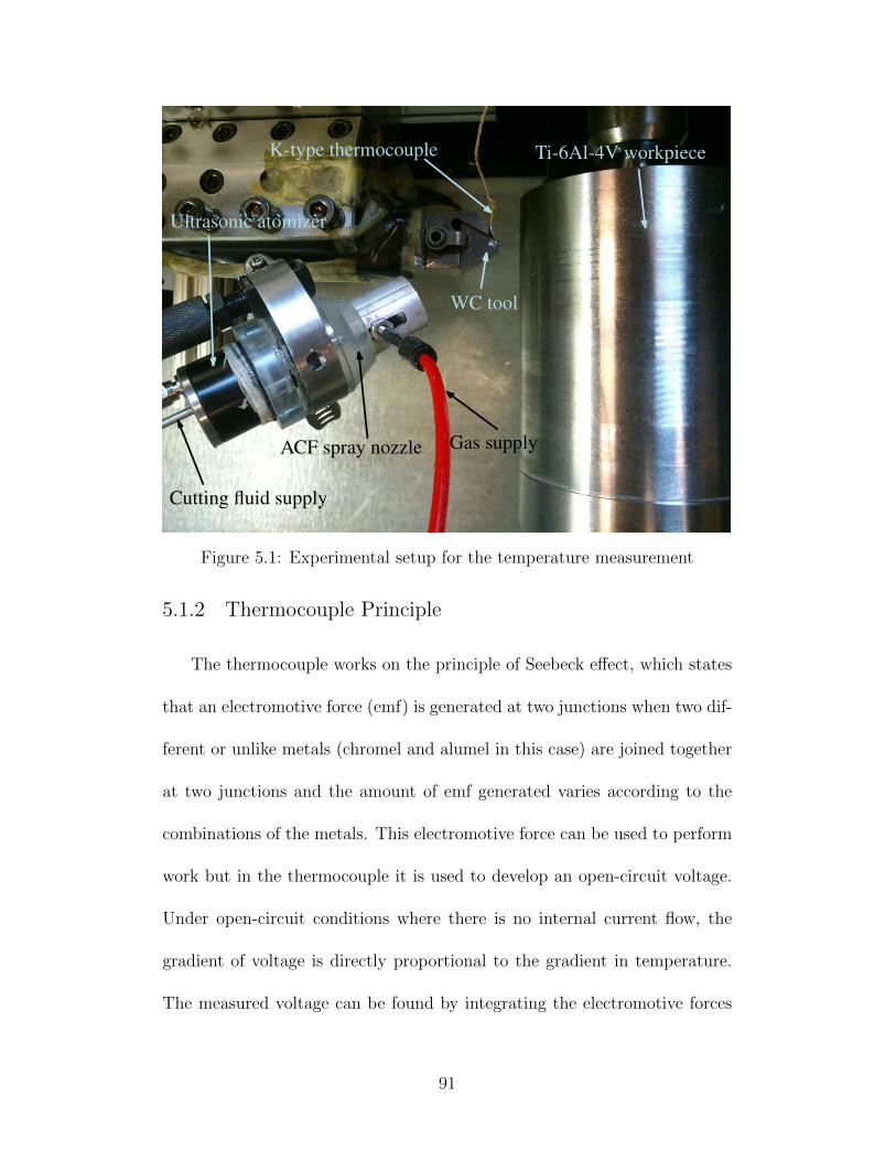
K-type thermocouple Ti-6Al-4V workpiece

WC tool

Gas supply

Cutting fluid supply

ACF spray nozzle

Ultrasonic atomizer

Figure 5.1: Experimental setup for the temperature measurement

5.1.2 Thermocouple Principle

The thermocouple works on the principle of Seebeck effect, which states

that an electromotive force (emf) is generated at two junctions when two dif-

ferent or unlike metals (chromel and alumel in this case) are joined together

at two junctions and the amount of emf generated varies according to the

combinations of the metals. This electromotive force can be used to perform

work but in the thermocouple it is used to develop an open-circuit voltage.

Under open-circuit conditions where there is no internal current flow, the

gradient of voltage is directly proportional to the gradient in temperature.

The measured voltage can be found by integrating the electromotive forces

91

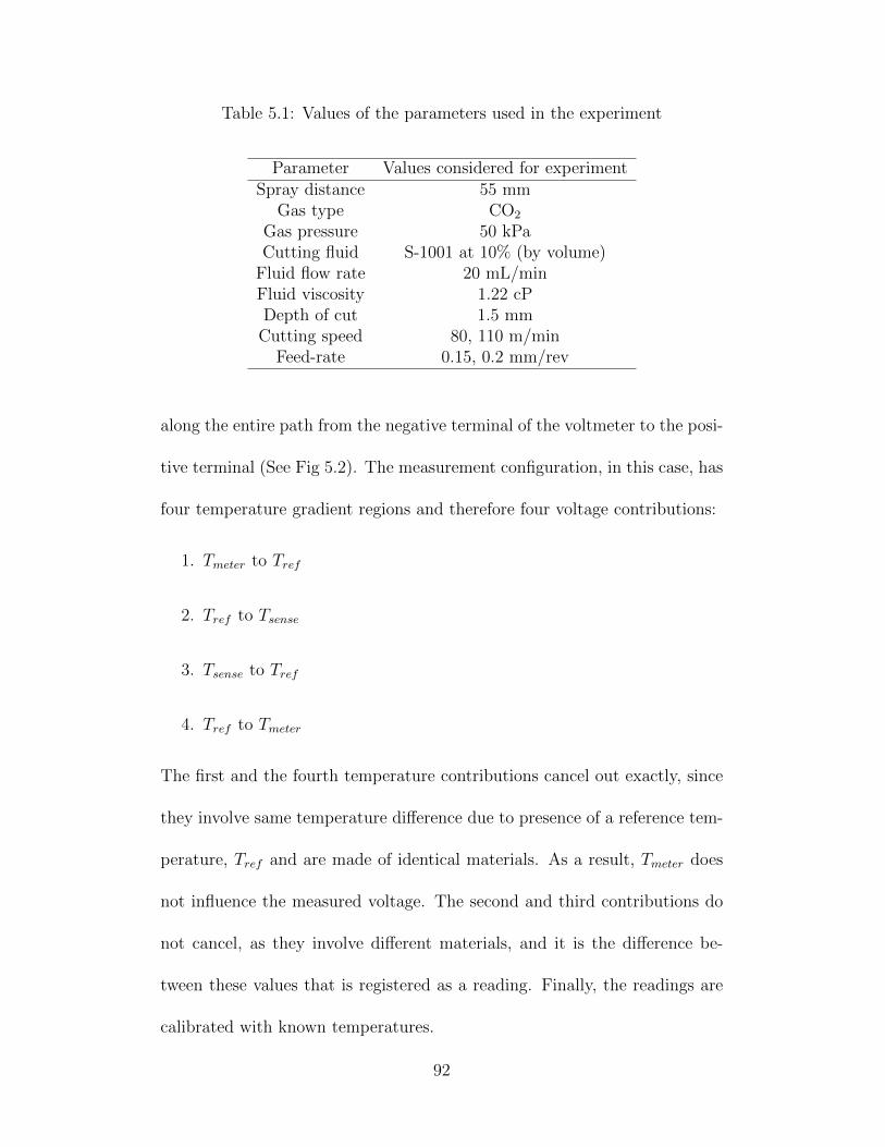
Table 5.1: Values of the parameters used in the experiment

Parameter Values considered for experimentSpray distance 55 mm

Gas type CO2

Gas pressure 50 kPaCutting fluid S-1001 at 10% (by volume)

Fluid flow rate 20 mL/minFluid viscosity 1.22 cPDepth of cut 1.5 mm

Cutting speed 80, 110 m/minFeed-rate 0.15, 0.2 mm/rev

along the entire path from the negative terminal of the voltmeter to the posi-

tive terminal (See Fig 5.2). The measurement configuration, in this case, has

four temperature gradient regions and therefore four voltage contributions:

1. Tmeter to Tref

2. Tref to Tsense

3. Tsense to Tref

4. Tref to Tmeter

The first and the fourth temperature contributions cancel out exactly, since

they involve same temperature difference due to presence of a reference tem-

perature, Tref and are made of identical materials. As a result, Tmeter does

not influence the measured voltage. The second and third contributions do

not cancel, as they involve different materials, and it is the difference be-

tween these values that is registered as a reading. Finally, the readings are

calibrated with known temperatures.

92

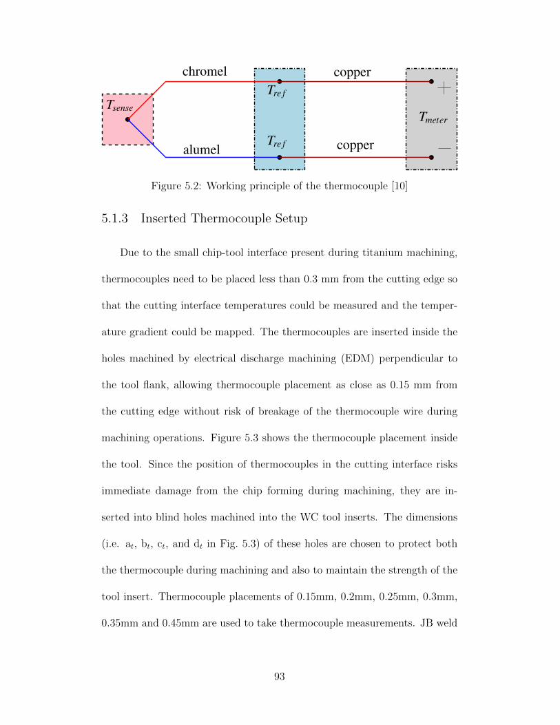
Tre f

Tre f

copper

copper

chromel

alumel

TsenseTmeter

Figure 5.2: Working principle of the thermocouple [10]

5.1.3 Inserted Thermocouple Setup

Due to the small chip-tool interface present during titanium machining,

thermocouples need to be placed less than 0.3 mm from the cutting edge so

that the cutting interface temperatures could be measured and the temper-

ature gradient could be mapped. The thermocouples are inserted inside the

holes machined by electrical discharge machining (EDM) perpendicular to

the tool flank, allowing thermocouple placement as close as 0.15 mm from

the cutting edge without risk of breakage of the thermocouple wire during

machining operations. Figure 5.3 shows the thermocouple placement inside

the tool. Since the position of thermocouples in the cutting interface risks

immediate damage from the chip forming during machining, they are in-

serted into blind holes machined into the WC tool inserts. The dimensions

(i.e. at, bt, ct, and dt in Fig. 5.3) of these holes are chosen to protect both

the thermocouple during machining and also to maintain the strength of the

tool insert. Thermocouple placements of 0.15mm, 0.2mm, 0.25mm, 0.3mm,

0.35mm and 0.45mm are used to take thermocouple measurements. JB weld

93

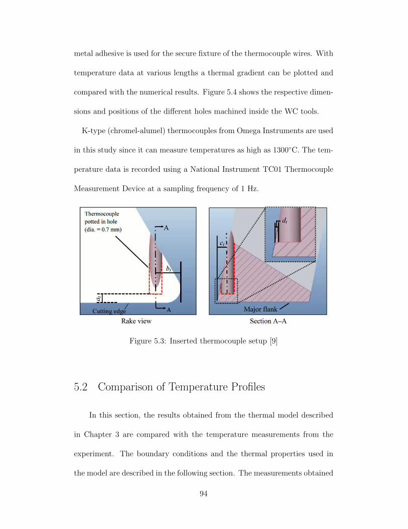
metal adhesive is used for the secure fixture of the thermocouple wires. With

temperature data at various lengths a thermal gradient can be plotted and

compared with the numerical results. Figure 5.4 shows the respective dimen-

sions and positions of the different holes machined inside the WC tools.

K-type (chromel-alumel) thermocouples from Omega Instruments are used

in this study since it can measure temperatures as high as 1300◦C. The tem-

perature data is recorded using a National Instrument TC01 Thermocouple

Measurement Device at a sampling frequency of 1 Hz.

Figure 5.3: Inserted thermocouple setup [9]

5.2 Comparison of Temperature Profiles

In this section, the results obtained from the thermal model described

in Chapter 3 are compared with the temperature measurements from the

experiment. The boundary conditions and the thermal properties used in

the model are described in the following section. The measurements obtained

94

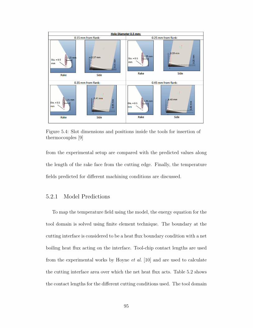
Figure 5.4: Slot dimensions and positions inside the tools for insertion ofthermocouples [9]

from the experimental setup are compared with the predicted values along

the length of the rake face from the cutting edge. Finally, the temperature

fields predicted for different machining conditions are discussed.

5.2.1 Model Predictions

To map the temperature field using the model, the energy equation for the

tool domain is solved using finite element technique. The boundary at the

cutting interface is considered to be a heat flux boundary condition with a net

boiling heat flux acting on the interface. Tool-chip contact lengths are used

from the experimental works by Hoyne et al. [10] and are used to calculate

the cutting interface area over which the net heat flux acts. Table 5.2 shows

the contact lengths for the different cutting conditions used. The tool domain

95

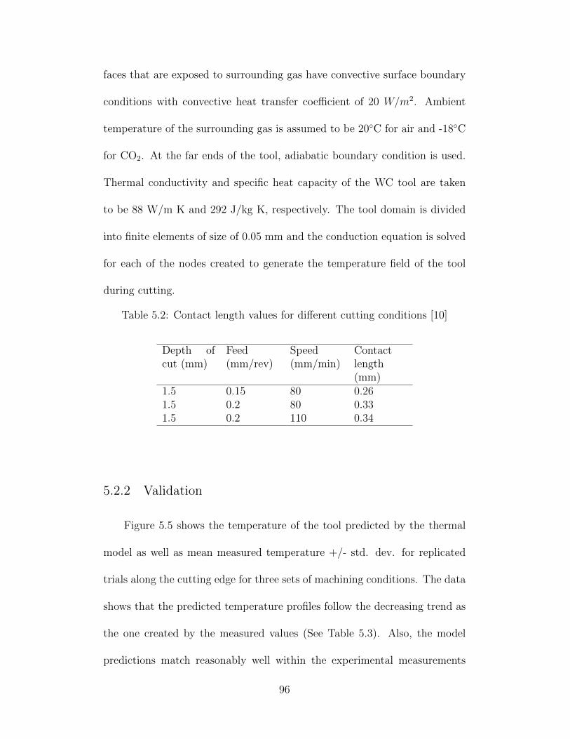
faces that are exposed to surrounding gas have convective surface boundary

conditions with convective heat transfer coefficient of 20 W/m2. Ambient

temperature of the surrounding gas is assumed to be 20◦C for air and -18◦C

for CO2. At the far ends of the tool, adiabatic boundary condition is used.

Thermal conductivity and specific heat capacity of the WC tool are taken

to be 88 W/m K and 292 J/kg K, respectively. The tool domain is divided

into finite elements of size of 0.05 mm and the conduction equation is solved

for each of the nodes created to generate the temperature field of the tool

during cutting.

Table 5.2: Contact length values for different cutting conditions [10]

Depth ofcut (mm)

Feed(mm/rev)

Speed(mm/min)

Contactlength(mm)

1.5 0.15 80 0.261.5 0.2 80 0.331.5 0.2 110 0.34

5.2.2 Validation

Figure 5.5 shows the temperature of the tool predicted by the thermal

model as well as mean measured temperature +/- std. dev. for replicated

trials along the cutting edge for three sets of machining conditions. The data

shows that the predicted temperature profiles follow the decreasing trend as

the one created by the measured values (See Table 5.3). Also, the model

predictions match reasonably well within the experimental measurements

96

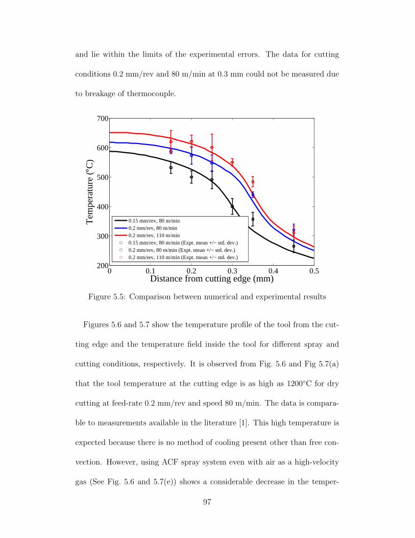
and lie within the limits of the experimental errors. The data for cutting

conditions 0.2 mm/rev and 80 m/min at 0.3 mm could not be measured due

to breakage of thermocouple.

0 0.1 0.2 0.3 0.4 0.5200

300

400

500

600

700

Distance from cutting edge (mm)

Tem

pera

ture

(°C)

0.15 mm/rev, 80 m/min0.2 mm/rev, 80 m/min0.2 mm/rev, 110 m/min0.15 mm/rev, 80 m/min (Expt. mean +/− std. dev.)0.2 mm/rev, 80 m/min (Expt. mean +/− std. dev.)0.2 mm/rev, 110 m/min (Expt. mean +/− std. dev.)

Figure 5.5: Comparison between numerical and experimental results

Figures 5.6 and 5.7 show the temperature profile of the tool from the cut-

ting edge and the temperature field inside the tool for different spray and

cutting conditions, respectively. It is observed from Fig. 5.6 and Fig 5.7(a)

that the tool temperature at the cutting edge is as high as 1200◦C for dry

cutting at feed-rate 0.2 mm/rev and speed 80 m/min. The data is compara-

ble to measurements available in the literature [1]. This high temperature is

expected because there is no method of cooling present other than free con-

vection. However, using ACF spray system even with air as a high-velocity

gas (See Fig. 5.6 and 5.7(e)) shows a considerable decrease in the temper-

97

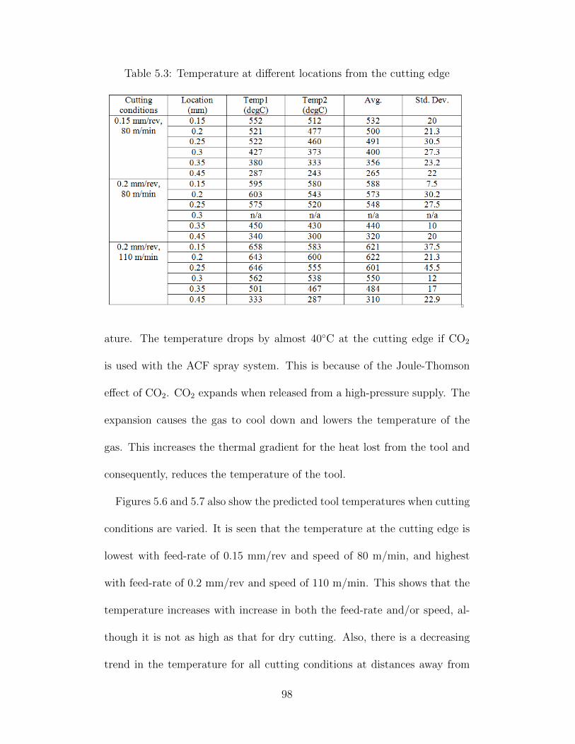
Table 5.3: Temperature at different locations from the cutting edge

ature. The temperature drops by almost 40◦C at the cutting edge if CO2

is used with the ACF spray system. This is because of the Joule-Thomson

effect of CO2. CO2 expands when released from a high-pressure supply. The

expansion causes the gas to cool down and lowers the temperature of the

gas. This increases the thermal gradient for the heat lost from the tool and

consequently, reduces the temperature of the tool.

Figures 5.6 and 5.7 also show the predicted tool temperatures when cutting

conditions are varied. It is seen that the temperature at the cutting edge is

lowest with feed-rate of 0.15 mm/rev and speed of 80 m/min, and highest

with feed-rate of 0.2 mm/rev and speed of 110 m/min. This shows that the

temperature increases with increase in both the feed-rate and/or speed, al-

though it is not as high as that for dry cutting. Also, there is a decreasing

trend in the temperature for all cutting conditions at distances away from

98

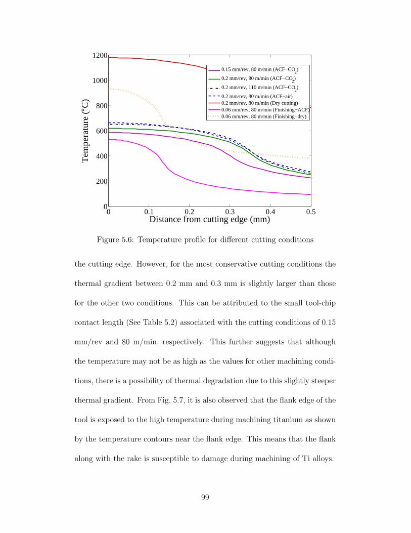
0 0.1 0.2 0.3 0.4 0.50

200

400

600

800

1000

1200

Distance from cutting edge (mm)

Tem

pera

ture

(°C)

0.15 mm/rev, 80 m/min (ACF−CO2)

0.2 mm/rev, 80 m/min (ACF−CO2)

0.2 mm/rev, 110 m/min (ACF−CO2)

0.2 mm/rev, 80 m/min (ACF−air)0.2 mm/rev, 80 m/min (Dry cutting)0.06 mm/rev, 80 m/min (Finishing−ACF)0.06 mm/rev, 80 m/min (Finishing−dry)

Figure 5.6: Temperature profile for different cutting conditions

the cutting edge. However, for the most conservative cutting conditions the

thermal gradient between 0.2 mm and 0.3 mm is slightly larger than those

for the other two conditions. This can be attributed to the small tool-chip

contact length (See Table 5.2) associated with the cutting conditions of 0.15

mm/rev and 80 m/min, respectively. This further suggests that although

the temperature may not be as high as the values for other machining condi-

tions, there is a possibility of thermal degradation due to this slightly steeper

thermal gradient. From Fig. 5.7, it is also observed that the flank edge of the

tool is exposed to the high temperature during machining titanium as shown

by the temperature contours near the flank edge. This means that the flank

along with the rake is susceptible to damage during machining of Ti alloys.

99

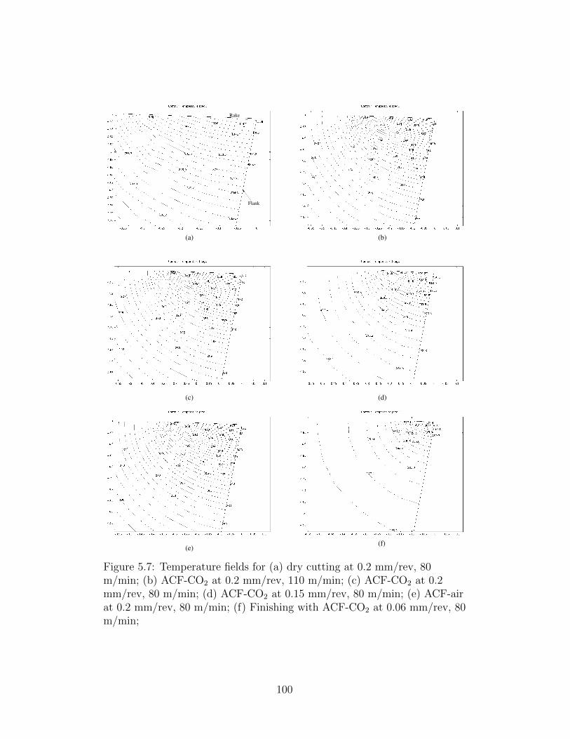
(a) (b)

(c) (d)

(e)(f)

Flank

Rake

Figure 5.7: Temperature fields for (a) dry cutting at 0.2 mm/rev, 80m/min; (b) ACF-CO2 at 0.2 mm/rev, 110 m/min; (c) ACF-CO2 at 0.2mm/rev, 80 m/min; (d) ACF-CO2 at 0.15 mm/rev, 80 m/min; (e) ACF-airat 0.2 mm/rev, 80 m/min; (f) Finishing with ACF-CO2 at 0.06 mm/rev, 80m/min;

100

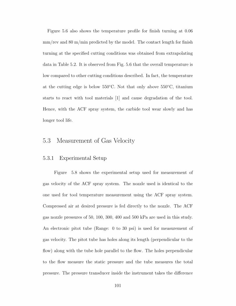
Figure 5.6 also shows the temperature profile for finish turning at 0.06

mm/rev and 80 m/min predicted by the model. The contact length for finish

turning at the specified cutting conditions was obtained from extrapolating

data in Table 5.2. It is observed from Fig. 5.6 that the overall temperature is

low compared to other cutting conditions described. In fact, the temperature

at the cutting edge is below 550◦C. Not that only above 550◦C, titanium

starts to react with tool materials [1] and cause degradation of the tool.

Hence, with the ACF spray system, the carbide tool wear slowly and has

longer tool life.

5.3 Measurement of Gas Velocity

5.3.1 Experimental Setup

Figure 5.8 shows the experimental setup used for measurement of

gas velocity of the ACF spray system. The nozzle used is identical to the

one used for tool temperature measurement using the ACF spray system.

Compressed air at desired pressure is fed directly to the nozzle. The ACF

gas nozzle pressures of 50, 100, 300, 400 and 500 kPa are used in this study.

An electronic pitot tube (Range: 0 to 30 psi) is used for measurement of

gas velocity. The pitot tube has holes along its length (perpendicular to the

flow) along with the tube hole parallel to the flow. The holes perpendicular

to the flow measure the static pressure and the tube measures the total

pressure. The pressure transducer inside the instrument takes the difference

101

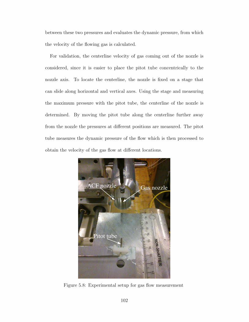
between these two pressures and evaluates the dynamic pressure, from which

the velocity of the flowing gas is calculated.

For validation, the centerline velocity of gas coming out of the nozzle is

considered, since it is easier to place the pitot tube concentrically to the

nozzle axis. To locate the centerline, the nozzle is fixed on a stage that

can slide along horizontal and vertical axes. Using the stage and measuring

the maximum pressure with the pitot tube, the centerline of the nozzle is

determined. By moving the pitot tube along the centerline further away

from the nozzle the pressures at different positions are measured. The pitot

tube measures the dynamic pressure of the flow which is then processed to

obtain the velocity of the gas flow at different locations.

Gas nozzleACF nozzle

Pitot tube

Figure 5.8: Experimental setup for gas flow measurement

102

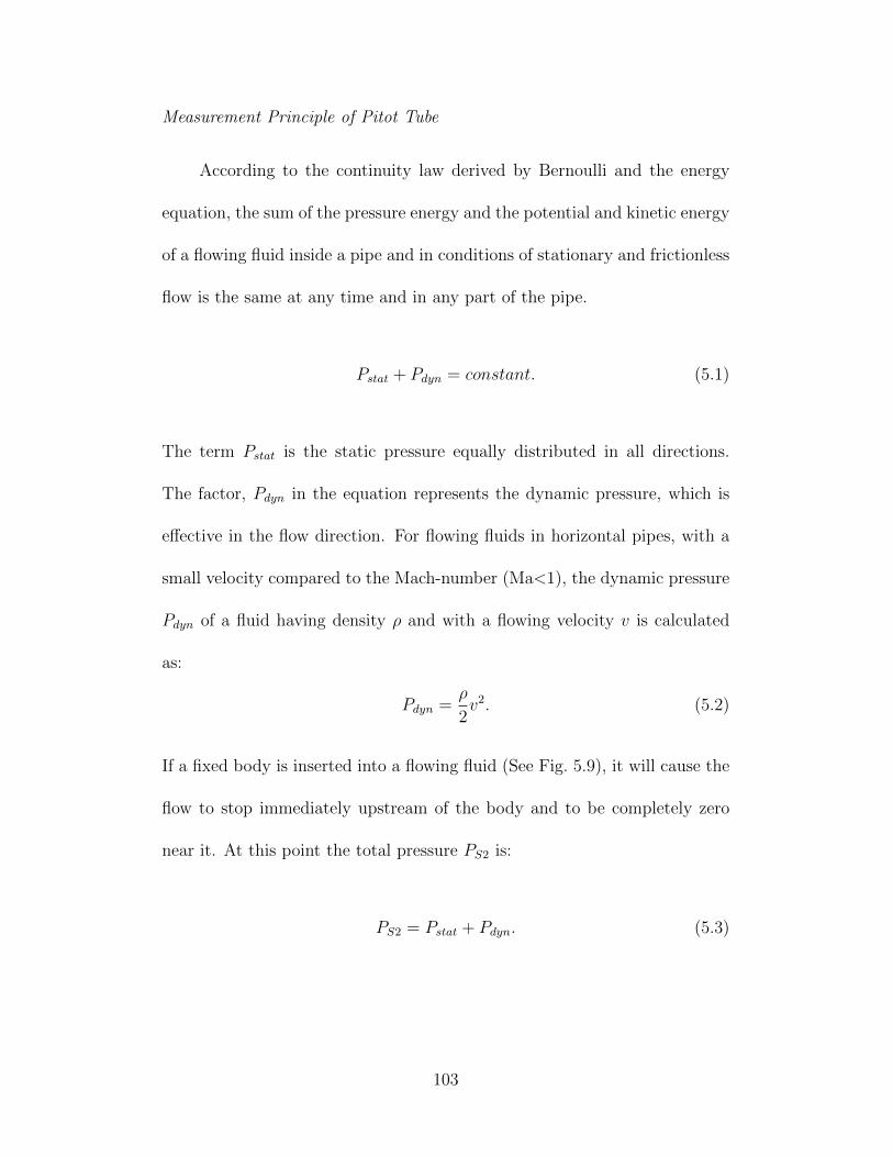
Measurement Principle of Pitot Tube

According to the continuity law derived by Bernoulli and the energy

equation, the sum of the pressure energy and the potential and kinetic energy

of a flowing fluid inside a pipe and in conditions of stationary and frictionless

flow is the same at any time and in any part of the pipe.

Pstat + Pdyn = constant. (5.1)

The term Pstat is the static pressure equally distributed in all directions.

The factor, Pdyn in the equation represents the dynamic pressure, which is

effective in the flow direction. For flowing fluids in horizontal pipes, with a

small velocity compared to the Mach-number (Ma<1), the dynamic pressure

Pdyn of a fluid having density ρ and with a flowing velocity v is calculated

as:

Pdyn =ρ

2v2. (5.2)

If a fixed body is inserted into a flowing fluid (See Fig. 5.9), it will cause the

flow to stop immediately upstream of the body and to be completely zero

near it. At this point the total pressure PS2 is:

PS2 = Pstat + Pdyn. (5.3)

103

In the downstream of the body, the sensors are only affected by the direction-

independent static pressure, Pstat. The difference in the upstream and down-

stream pressures, the differential pressure ∆P , is then a measure of the ve-

locity with which the inserted body is impacted:

∆P = PS2 − Pstat (5.4)

Substituting Eq. 5.3 into Eq. 5.4, the velocity of flow can be obtained:

v =

√2∆P

ρ(5.5)

Gas Flow

PS2 PstatBody

Figure 5.9: Working principle of the pitot tube

5.3.2 Comparison of Gas Velocity Profiles

The velocity contour of gas obtained from the simulation are shown

in Fig. 5.10 for different gas nozzle pressures. The gas exits the converging

nozzle and due to the large pressure difference between the inlet pressure and

the ambient pressure, the gas reaches a very high velocity right after the exit

104

from the nozzle. This is expected since the sudden decrease in pressure is

accompanied by the increase in velocity to conserve energy. It is observed

that the overall gas flow velocity increases with increase in the inlet pressure.

Further downstream, the velocity decreases but the area over which this high

velocity gas influences increases. This is caused by the developing shear layer.

Figure 5.11 compares the velocity of gas predicted from the spray model

with the experimental values along the centerline of the ACF spray system

(See Fig. 4.2). The centerline velocity starting from the mouth of the ACF

spray nozzle to the surface of the tool is validated only since the velocity

within that distance is of general interest to determine where the spreading

regime velocity occurs. For a given pressure, the gas velocity decreases as

distance from the ACF spray system is increased. This is expected as energy

gets dissipated to the surrounding and the gas settles down to atmospheric

condition. As can be seen for Fig. 5.11, the results from the model closely

match the experimental findings with a maximum discrepancy of 11% for all

conditions tested.

5.4 Chapter Summary

In summary, it has been observed that the temperature profile predicted

by the thermal model closely match with the temperature data obtained from

the experimental measurements. For cutting conditions of 0.15 mm/rev and

105

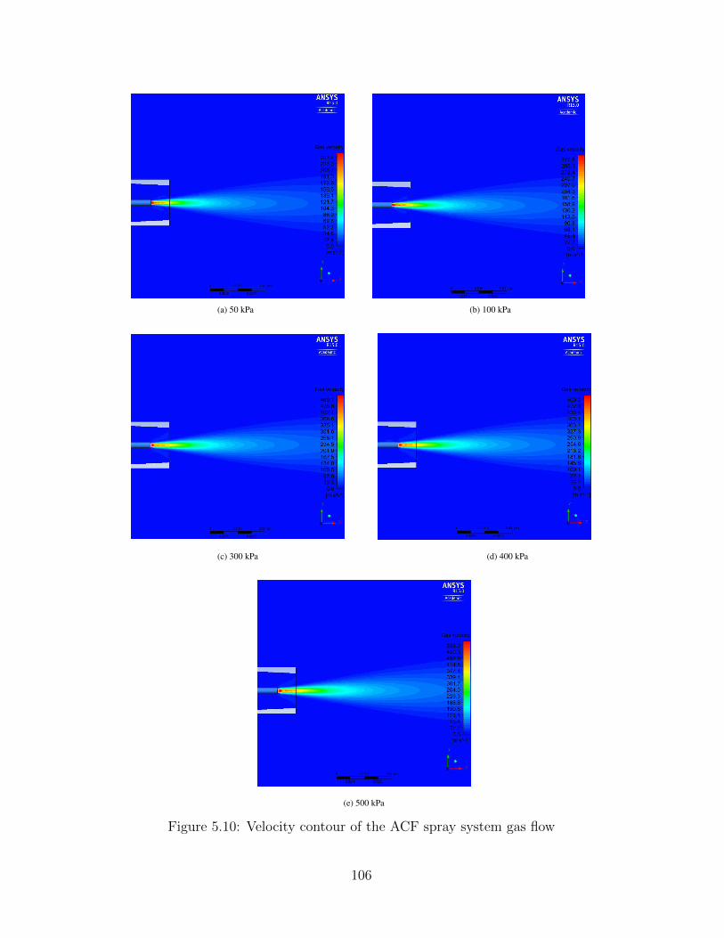
(a) 50 kPa (b) 100 kPa

(c) 300 kPa (d) 400 kPa

(e) 500 kPa

Figure 5.10: Velocity contour of the ACF spray system gas flow

106

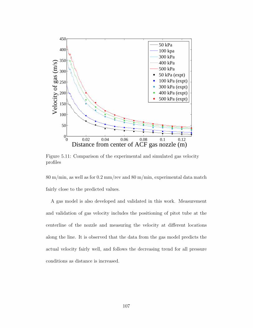
0 0.02 0.04 0.06 0.08 0.1 0.120

50

100

150

200

250

300

350

400

450

Distance from center of ACF gas nozzle (m)

Vel

ocity

of

gas

(m/s

)

50 kPa100 kpa300 kPa400 kPa500 kPa50 kPa (expt)100 kPa (expt)300 kPa (expt)400 kPa (expt)500 kPa (expt)

Figure 5.11: Comparison of the experimental and simulated gas velocityprofiles

80 m/min, as well as for 0.2 mm/rev and 80 m/min, experimental data match

fairly close to the predicted values.

A gas model is also developed and validated in this work. Measurement

and validation of gas velocity includes the positioning of pitot tube at the

centerline of the nozzle and measuring the velocity at different locations

along the line. It is observed that the data from the gas model predicts the

actual velocity fairly well, and follows the decreasing trend for all pressure

conditions as distance is increased.

107

CHAPTER 6

CONCLUSIONS ANDRECOMMENDATIONS

6.1 Summary

The work presented in this thesis develops a thermal model that simulates

the cooling effect due to ACF spray system in machining by incorporating

film boiling of droplets. The research also determines the spray parameters

through a CFD study for which the droplets formed from the ACF spray

system will spread on the heated surface of the tool and therefore, contribute

to the heat transfer.

To develop the thermal model, a controlled experiment is conducted at

first to observe the heat transfer phenomenon that is likely to take place at

the cutting interface at high machining temperatures. A tool is heated to

over 300◦C and the cutting fluid from the ACF system is sprayed on it. It

is observed that boiling heat transfer phenomenon is the dominant form of

heat transfer at that temperature. The thermal model is developed with an

impinged droplet cushioned over a thin vapor film to replicate the Leidenfrost

effect in film boiling. It is through this thin vapor film that heat is conducted

away from the tool. Using equations of mass and momentum, the thickness

108

of the film is first determined and the net heat flux acting on the cutting

interface is evaluated and the temperature field of the tool is obtained.

In the spray model, ACF spray parameters are determined for which the

droplets being impinged on the surface of the tool are within the spreading

regime velocity. Using CFD technique, a gas flow velocity profile is created

that simulates the gas nozzle velocity for a given pressure. Cutting fluid

droplets are then introduced to the flow field and the resultant velocity of

the droplets are evaluated. For a given pressure and droplet size, the spray

distance range within which the velocity falls within the spreading range is

determined. This ensures that the droplet spreads upon impact with the tool

surface and introduce film boiling heat transfer.

6.2 Conclusions

In this study, a thermal model based on the film boiling heat transfer is

developed to predict the tool temperature at the cutting edge and map the

temperature field in the tool. Additionally, a spray model to determine the

minimum spray distance to ensure droplets spread on the heated surface has

been formulated. Based on the analyses made from the model results, the

following conclusions can be drawn.

1. Boiling is one of the principal heat transfer mechanisms that take place

during ACF spray cooling. With tool temperature much above 600◦C,

film boiling is assumed to take place near the cutting edge. The model

109

considers heat conduction through the vapor layer formed by film boil-

ing. This work also takes into account the variation of surface temper-

ature in the model unlike most works in literature, where the temper-

ature is assumed to be constant.

2. Due to the high temperature involved at the cutting interface, the

cutting-fluid spray from the ACF spray system forms droplets on the

heated surface and contributes to the cooling by film boiling heat trans-

fer.

3. The predicted temperature profiles follow the decreasing trend as also

seen for the measured data. Also, the model predictions match rea-

sonably well within the experimental measurements and lie within the

limits of the experimental errors.

4. The temperature field in the tool provided by the model for dry cutting

shows that the cutting edge temperature is almost twice as high as

compared to that with ACF spray for cutting conditions of 0.15 mm/rev

and 80 m/min.

5. In the ACF spray cooling, the CO2 gas expands when released from the

nozzle and lowers the ambient temperature of the tool. This increases

the temperature difference between the tool surface and the surround-

ing and as a result, enhances the heat transfer rate. The result of this

Joule-Thompson effect of CO2 enables the ACF spray system to reduce

110

the tool temperature more effectively.

6. Cutting conditions including feed-rate and speed influence the maxi-

mum temperature at the cutting edge for machining with ACF spray

cooling. However, the temperatures are not as drastically high as in

dry cutting.

7. In finish turning of titanium alloy, the ACF spray system provides a

cooling effect to keep the cutting temperature below 550◦C. As a result,

the carbide tool can survive longer without having any significant wear.

8. The spray model that takes into account both the gas flow and the

droplet flow is able to demonstrate the entrainment of droplets in the

gas jet stream. In addition, it is also able to predict the droplet ve-

locities for a given gas nozzle pressure and droplet size over the spray

distance. This helps in determining the distance range at which droplet

reaches the spreading regime velocity and is able to contribute to the

heat transfer on the heated surface.

9. Droplet size range of 12.5-30 µm has been observed to be suitable for

providing a large range in spray distance in the ACF spray system.

Increasing the droplet size will narrow the velocity range required for

spreading of the droplet.

111

6.3 Recommendations for Future Work

Below are suggestions for extending the research in order to better predict

the temperature of the tool when machining with the ACF spray system.

1. The temperature of the tool is as high as 600◦C. As the surface tem-

perature is increased, radiation through the vapor film becomes more

significant and the heat flux increases with increasing excess tempera-

ture. A model that would include the heat transfer due to radiation is

needed.

2. The model could predict the tool temperature profile more accurately

if a distribution of the droplets impinging on the surface could be de-

termined. A Rosin-Rammler distribution could be introduced to deter-

mine the droplet size and number distribution. By accounting for the

number of droplets on an interface area, the temperature of the cutting

interface could be better determined.

3. The thermal model should be enhanced to include the solid-fluid in-

teraction between the chip and the droplet. Since, the chip also takes

away some heat from the shear zones, involving the geometry of the chip

could help predict the temperature of the tool more accurately. This

could be done by using a finite element model where the chip is gen-

erated from the workpiece by introducing machining conditions. The

thermal model could then be incorporated with the resultant domain

112

to achieve the temperature field.

4. It is assumed in this study that the heat transfer problem is a quasi-

steady state one. However, in reality the boiling heat transfer is a

result of the constant evaporation of the whole droplet and regener-

ation of new droplets from the droplet source. The model should be

improved by considering the whole transient process from the point of

impingement to the complete evaporation of droplets.

5. Further studies should be carried out to determine effect of cutting

fluid viscosity on the ACF spray system cooling by varying the fluid

properties in the thermal model. Such a study should also investigate

the effectiveness of less-hazardous cutting fluids, for e.g. vegetable oil.

6. The thermal model could be applied in machining for predicting tool

temperature for other hard-to-machine materials that experience simi-

lar temperature-related wear issues as titanium and its alloys. Such a

study could reveal any difference in the cooling mechanism for different

materials.

113

REFERENCES

[1] E. Ezugwu and Z. Wang, “Titanium alloys and their machinability,”Journal of Materials Processing Technology, vol. 68, pp. 262–274, 1997.

[2] A. Machado and J. Wallbank, “Machining of titanium and its alloys - areview,” pp. 53–60, 1990.

[3] R. R. Boyer, “An overview on the use of titanium in the aerospaceindustry,” Materials Science and Engineering A, vol. 213, no. 1-2, pp.103–114, 1996.

[4] Y. Li, C. Yang, H. Zhao, S. Qu, X. Li, and Y. Li, “New developmentsof ti-based alloys for biomedical applications,” Materials, vol. 7, pp.1709–1800, 2014.

[5] M. Peters and J. Kumpfert, “Titanium alloys for aerospace applica-tions,” Advanced Engineering . . . , vol. 5, pp. 419–427, 2003.

[6] a. K. Nandy, M. C. Gowrishankar, and S. Paul, “Some studies on high-pressure cooling in turning of Ti-6Al-4V,” International Journal of Ma-chine Tools and Manufacture, vol. 49, no. 2, pp. 182–198, 2009.

[7] C. Nath, S. G. Kapoor, A. K. Srivastava, and J. Iverson, “Study ofDroplet Spray Behavior of an Atomization-Based Cutting Fluid SpraySystem for Machining Titanium Alloys,” Journal of Manufacturing Sci-ence and Engineering, vol. 136, no. 2, p. 021004, Jan. 2014.

[8] M. B. G. Jun, S. S. Joshi, R. E. DeVor, and S. G. Kapoor, “An Exper-imental Evaluation of an Atomization-Based Cutting Fluid ApplicationSystem for Micromachining,” Journal of Manufacturing Science and En-gineering, vol. 130, no. 3, p. 031118, 2008.

[9] A. C. Hoyne, C. Nath, and S. G. Kapoor, “Characterization of FluidFilm Produced by an Atomization-Based Cutting Fluid Spray SystemDuring Machining,” Journal of Manufacturing Science and Engineering,vol. 135, no. 5, p. 051006, Sep. 2013.

[10] A. C. Hoyne, C. Nath, and S. G. Kapoor, “Cutting Temperature Mea-surement During Titanium Machining with an Atomization-based Cut-ting Fluid (ACF) Spray System,” IMECE, 2013.

114

[11] U. T. M. R. M. B. Davies, M.A. and A. Cooke, “On the measurement oftemperature in material removal processes,” Annals of CERP, vol. 56,pp. 581–604, 2007.

[12] E. Loewen and M. Shaw, “On the analysis of cutting tool temperatures,”Transactions of ASME, vol. 76, pp. 217–231, 1954.

[13] J. Weiner, “Shear plane temperature distribution in orthogonal cutting,”Transactions of ASME, vol. 77, p. 1331, 1954.

[14] R. Radulescu, “Dynamic modeling of machining processes using a finiteelement approach,” M.S. Thesis, UIUC, 1991.

[15] A. U. Anagonye and D. a. Stephenson, “Modeling Cutting Tempera-tures for Turning Inserts With Various Tool Geometries and Materials,”Journal of Manufacturing Science and Engineering, vol. 124, p. 544,2002.

[16] R. Li and A. Shih, “Finite element modeling of 3D turning of titanium,”International Journal of Advanced Manufacturing Technology, vol. 29,pp. 253–261, 2006.

[17] M. Sima and Ozel.T, “Modified material constitutive models for serratedchip formation simulations and experimental validation in machining oftitanium alloy Ti-6Al-4V,” International Journal of Machine Tools andManufacture, vol. 50, pp. 943–960, 2010.

[18] Y. Karpat, “Temperature dependent flow softening of titanium alloyTi6Al4V An investigation using finite element simulation of machining,”Journal of Materials Processing Technology, vol. 211, pp. 737–749, 2011.

[19] T. Thepsonthi and T. Ozel, “Experimental and finite element simulationbased investigations on micro-milling Ti-6Al-4V titanium alloy: Effectsof cBN coating on tool wear,” Journal of Materials Processing Technol-ogy, vol. 213, pp. 532–542, Apr. 2013.

[20] S. Pervaiz, I. Deiab, E. M. Ibrahim, A. Rashid, and M. Nicolescua, “Acoupled FE and CFD approach to predict the cutting tool temperatureprofile in machining,” Procedia CIRP, vol. 17, pp. 750–754, 2014.

[21] Z. Zhao, D. Poulikakos, and J. Fukai, “Heat transfer and fluid dynamicsduring the collision of a liquid droplet on a substrateI. Modeling,” In-ternational Journal of Heat and Mass Transfer, vol. 39, pp. 2771–2789,1996.

[22] M. C. Ece and A. Ozturk, “Modelling unsteady convective heat transferfor fuel droplets,” Energy Conversion and Management, vol. 48, pp.689–692, 2007.

115

[23] A. Q. M. Sazhin, S. S., R. Kolodnytska, N. R. Elwardany, a.E., and M. R.Heikal, “Modelling of biodiesel fuel droplet heating and evaporation,”Fuel, vol. 115, pp. 559–572, 2014.

[24] Y. Ge and L. S. Fan, “3-D modeling of the dynamics and heat trans-fer characteristics of subcooled droplet impact on a surface with filmboiling,” International Journal of Heat and Mass Transfer, vol. 49, pp.4231–4249, 2006.

[25] S. Nishio and Y. C. Kim, “Heat transfer of dilute spray impinging onhot surface (simple model focusing on rebound motion and sensible heatof droplets),” International Journal of Heat and Mass Transfer, vol. 41,pp. 4113–4119, 1998.

[26] J. D. Bernardin and I. Mudawar, “Transition Boiling Heat Transfer ofDroplet Streams and Sprays,” Journal of Heat Transfer, vol. 129, p.1605, 2007.

[27] D. Stephenson and J. Agapiou, “Metal cutting theory and practice,”2006.

[28] B. Bannon and E. Mild, “Titanium Alloys for Biomaterial Application:An Overview. Titanium,” Titanium Alloys in Surgical Implants; ASTM,pp. 7–15, 1983.

[29] D. Williams, “On the mechanisms of biocompatibility,” Biomaterials,vol. 29, pp. 2941–2953, 2008.

[30] d.-W. J. v.-B. C. Li, J.P. and K. de Groot, “Porous Ti6Al4V scaffolddirectly fabricating by rapid prototyping: Preparation and in vitro ex-periment,” Biomaterials, vol. 27, p. 12231235, 2006.

[31] N. Zlatin and M. Field, “Procedures and precautions in machining tita-nium alloys,” pp. 489–504, 1973.

[32] S. Sun, M. Brandt, and M. Dargusch, “Characteristics of cutting forcesand chip formation in machining of titanium alloys,” International Jour-nal of Machine Tools and Manufacture, vol. 49, pp. 561–568, 2009.

[33] J. Balaji, V. Krishnaraj, and S. Yogeswaraj, “Investigation on HighSpeed Turning of Titanium Alloys,” Procedia Engineering, vol. 64, pp.926–935, 2013.

[34] F. H. F. J. F. Kahles, D. Eylon and M. Field, “Machining of TitaniumAlloys,” Journal of Metals, vol. 37, pp. 27–35, 1985.

[35] Q. Shi, L. Li, N. He, W. Zhao, and X. Liu, “Experimental study inhigh speed milling of titanium alloy tc21,” The International Journal ofAdvanced Manufacturing Technology, vol. 64, pp. 49–54, 2013.

116

[36] S. Vijay and V. Krishnaraj, “Machining Parameters Optimization inEnd Milling of Ti-6Al-4V,” Procedia Engineering, vol. 64, pp. 1079–1088, 2013.

[37] W. Konig, “Applied research on the machinability of titanium and itsalloys,” Proc. 47th Meeting of AGARD Structural and Materials Panel,vol. 202, pp. 1.1–1.10, 1979.

[38] P. Dearnley and A. Grearson, “Evaluation of principal wear mechanismsof cemented carbides and ceramics used for machining titanium alloy IMI318,” Materials Science and Technology, vol. 2, pp. 47–58, 1986.

[39] N. Narutaki, “Study on Machining of Titanium Alloys,” Cirp Annals-manufacturing Technology, vol. 32, pp. 65–69, 1983.

[40] T. Kitagawa, a. Kubo, and K. Maekawa, “Temperature and wear ofcutting tools in high-speed machining of Incone1718 and Ti-6A1-6V-2Sn,” Wear, vol. 202, no. 2, pp. 142–148, 1997.

[41] P. Benardos and G.-C. Vosniakos, “Predicting surface roughness in ma-chining: a review,” International Journal of Machine Tools and Manu-facture, vol. 43, no. 8, pp. 833 – 844, 2003.

[42] C. H. Che-Haron, “Tool life and surface integrity in turning titaniumalloy,” Journal of Materials Processing Technology, vol. 118, pp. 231–237, 2001.

[43] a. K. M. N. Amin, A. F. Ismail, and M. K. Nor Khairusshima, “Effec-tiveness of uncoated WC-Co and PCD inserts in end milling of titaniumalloy-Ti-6Al-4V,” Journal of Materials Processing Technology, vol. 192-193, pp. 147–158, 2007.

[44] J. Hua and R. Shivpuri, “Prediction of chip morphology and segmen-tation during the machining of titanium alloys,” Journal of MaterialsProcessing Technology, vol. 150, pp. 124–133, 2004.

[45] U. K. Ueda N, Matsuo T, “An analysis of saw-toothed chip formation,”CIRP Ann Manuf Technol, vol. 31, pp. 81–84, 1982.

[46] D. B. J. H. R. Konmanduri, T.A. Schroeder, “Titanium: a model ma-terial for analysis of the high-speed machining process, advanced pro-cessing methods for titanium, in: D.f. hasson, c.h. hamilton (eds.),” TheMetallurgical Society of ASME, pp. 241–256.

[47] A. Li, J. Zhao, Y. Zhou, X. Chen, and D. Wang, “Experimental investi-gation on chip morphologies in high-speed dry milling of titanium alloyTi-6Al-4V,” International Journal of Advanced Manufacturing Technol-ogy, vol. 62, pp. 933–942, 2012.

117

[48] S. Palanisamy, S. D. McDonald, and M. S. Dargusch, “Effects of coolantpressure on chip formation while turning Ti6Al4V alloy,” InternationalJournal of Machine Tools and Manufacture, vol. 49, pp. 739–743, 2009.

[49] S. Y. Hong and Y. Ding, “Cooling approaches and cutting temperaturesin cryogenic machining of Ti-6Al-4V,” International Journal of MachineTools and Manufacture, vol. 41, pp. 1417–1437, 2001.

[50] K. a. Venugopal, S. Paul, and a. B. Chattopadhyay, “Tool wear in cryo-genic turning of Ti-6Al-4V alloy,” Cryogenics, vol. 47, pp. 12–18, 2007.

[51] A. Cardoni, Power Ultrasonics. Elsevier Ltd., 2010, vol. 57.

[52] D. Sindayihebura, M. Dobre, and L. Bolle, “Experimental study of thinliquid film ultrasonic atomization,” 4th World Conference on Experi-mental Heat Transfer, Fluid Mechanics and Thermodynamics, pp. 1249–1256, 1997.

[53] M. Rukosuyev, C. S. Goo, and M. B. G. Jun, “Understanding the effectsof the system parameters of an ultrasonic cutting fluid application sys-tem for micro-machining,” Journal of Manufacturing Processes, vol. 12,no. 2, pp. 92–98, 2010.

[54] “Spray-combustion interaction mechanism of multiple-injection underdiesel engine conditions,” Proceedings of the Combustion Institute,vol. 35, no. 3, pp. 3061–3068, 2014.

[55] R. Payri, A. Garcıa, V. Domenech, R. Durrett, and A. H. Plazas, “Anexperimental study of gasoline effects on injection rate, momentum fluxand spray characteristics using a common rail diesel injection system,”Fuel, vol. 97, pp. 390–399, 2012.

[56] M. Rein, “Phenomena of liquid drop impact on solid and liquid sur-faces,” Fluid Dynamics Research, vol. 12, no. 2, pp. 61–93, 1993.

[57] W. Zhou, D. Loney, A. G. Ferorov, F. L. Degertekin, and D. W. Rosen,“Shape Characterization for Droplet Impingement Dynamics in Ink-JetDeposition,” pp. 1–7, 2015.

[58] A. Yarin, “Drop Impact Dynamics: Splashing, Spreading, Receding,Bouncing...” Annual Review of Fluid Mechanics, vol. 38, no. 1, pp. 159–192, 2006.

[59] D. W. Stanton and C. J. Rutland, “Multi-dimensional modeling of thinliquid films and spray-wall interactions resulting from impinging sprays,”International Journal of Heat and Mass Transfer, vol. 41, no. 20, pp.3037–3054, Oct. 1998.

118

[60] K. Range and F. Feuillebois, “Influence of Surface Roughness on LiquidDrop Impact,” Journal of Colloid and Interface Science, vol. 203, no.203, pp. 16–30, 1998.

[61] A. V. Mahulkar, G. B. Marin, and G. J. Heynderickx, “Dropletwall in-teraction upon impingement of heavy hydrocarbon droplets on a heatedwall,” Chemical Engineering Science, vol. 130, pp. 275–289, 2015.

[62] O. W. Jayaratne and B. J. Mason, “The coalescence and bouncing ofwater drops at an air/water interface,” Proceedings of the Royal Societyof London A: Mathematical, Physical and Engineering Sciences, vol. 280,no. 1383, pp. 545–565, 1964.

[63] C. D. Stow and M. G. Hadfield, “An experimental investigation of fluidflow resulting from the impact of a water drop with an unyielding drysurface,” Proceedings of the Royal Society of London A: Mathematical,Physical and Engineering Sciences, vol. 373, no. 1755, pp. 419–441, 1981.

[64] C. Mundo, M. Sommerfield, and C. Tropea, “Droplet - Wall Collisions :Experimental Studies of the Deformation and Breakup Process,” vol. 21,no. 2, 1995.

[65] C. X. Bai, H. Rusche, and a. D. Gosman, “Modeling of Gasoline SprayImpingment,” pp. 1–27, 2002.

[66] A. L. N. Moreira, A. S. Moita, and M. R. Panao, “Advances and chal-lenges in explaining fuel spray impingement: How much of single dropletimpact research is useful?” Progress in Energy and Combustion Science,vol. 36, pp. 554–580, 2010.

[67] J. Fukai, Y. Shiiba, T. Yamamoto, O. Miyatake, D. Poulikakos, C. M.Megaridis, and Z. Zhao, “Wetting effects on the spreading of a liquiddroplet surface : Experiment and modeling colliding with a flat,” Physicsof Fluids, vol. 7, pp. 236–247, 1995.

[68] I. Ghai, J. Wentz, R. E. DeVor, S. G. Kapoor, and J. Samuel, “DropletBehavior on a Rotating Surface for Atomization-Based Cutting FluidApplication in Micromachining,” Journal of Manufacturing Science andEngineering, vol. 132, p. 011017, 2010.

[69] D. a. Weiss and A. L. Yarin, “Single drop impact onto liquid films:neck distortion, jetting, tiny bubble entrainment, and crown formation,”Journal of Fluid Mechanics, vol. 385, pp. 229–254, 1999.

[70] K. J. Trigger and B. T. Chao, “An Analytical Evaluation of Metal Cut-ting Temperatures,” Trans. ASME, vol. 73, pp. 57–58, 1951.

119

[71] B. Abramzon and W. Sirignano, “Droplet vaporization model for spraycombustion calculations,” International Journal of Heat and MassTransfer, vol. 32, pp. 1605–1618, 1989.

[72] N. Abukhshim, P. Mativenga, and M. Sheikh, “Investigation of heatpartition in high speed turning of high strength alloy steel,” Interna-tional Journal of Machine Tools and Manufacture, vol. 45, pp. 1687–1695, 2005.

[73] B. Incropera, DeWitt and Lavine, Fundamentals of Heat and MassTransfer, 6th edition.

[74] O. G. Engel, “Waterdrop Collision with Solid Surface,” J. Res. Natn.Bur. Stand., vol. 54, p. 281, 1955.

[75] R. E. Ford and C. G. L. Furmidge, “Impact and Spreading of SprayDrops on Foliar Surfaces,” Wetting. Soc. Chem. Industry Monograph, p.417, 1967.

[76] H. Park, W. Carr, J. Zhu, and J. Morris, “Single drop impaction ona solid surface,” Fluids Mechanics and Transport Phenomena, vol. 49,no. 10, pp. 2461–2471, 2003.

[77] M. Pasandideh-Fard, Q. Y. M., S. Chandra, and J. Mostaghimi, “Capil-lary effects during droplet impact on a solid surface,” Physics of Fluids(1994-present), vol. 8, no. 3, pp. 650–659, 1996.

[78] T. Mao, D. C. S. Kuhn, and H. Tran, “Spread and rebound of liquiddroplets upon impact on flat surfaces,” AIChE Journal, vol. 43, no. 9,pp. 2169–2179, 1997.

[79] T. S. Chow, “Wetting of rough surfaces,” Journal of Physics: CondensedMatter, vol. 10, p. L445, 1998.

[80] D. C. Wilcox, “Formulation of the k-w Turbulence Model Revisited,”AIAA Journal, vol. 46, pp. 2823–2838, 2008.

[81] “Ansys fluent,” http://www.arc.vt.edu/ansys help.

[82] D. M. A. B. Liu and R. D. Reitz, “Modeling the Effects of Drop Dragand Breakup on Fuel Sprays,” SAE Technical Paper 930072, 1993.

120