c© 2018 by Jonathan Morgan. All rights reserved.

PREDICTION OF FLIGHT MEASUREMENTS OF HIGH ENTHALPYNONEQUILIBRIUM FLOW FROM A CUBESAT-CLASS ATMOSPHERIC PROBE

BY

JONATHAN MORGAN

THESIS

Submitted in partial fulfillment of the requirementsfor the degree of Master of Science in Aerospace Engineering

in the Graduate College of theUniversity of Illinois at Urbana-Champaign, 2018

Urbana, Illinois

Advisor:Professor Deborah Levin

Abstract

Spectral radiation is sensitive to many physical chemical aspects of high-enthalpy, non-equilibrium flows

affect radiation and heat transfer estimates at low-earth altitudes, which is important as a flow diagnostic.

For diatomic molecules, high energy collisions in the bow shock region result in ro-vibrionic transitions

and release of photons in different wavelength bands. In this work, the Direct Simulations Monte Carlo

(DSMC) method is used for the SASSI2 mission to determine the external flow field around a 3U CubeSat

and the internal flowfield of custom pressure sensor ports. The Nonequilibrium Radiative Transport and

Spectra Program (NEQAIR) code is used to determine ultraviolet radiation from nitric oxide and the tangent

slab approximation is used to estimate spacecraft visible glow radiance from nitrogen dioxide. Additional

calculations are performed to provide a sensitivity analysis of radiance estimates based on the DSMC code

utilized, chemical reaction rates, and CubeSat orientation.

ii

To my mother and father.

iii

Acknowledgments

This project would not have been possible without the support of many people. Many thanks to my advisor,

Dr. Deborah Levin, who read my numerous revisions and helped make sense of the confusion. Thanks to

Rose who endured this long process with me, always offering support and love.

iv

Table of Contents

List of Tables . . . . . . . . . . . . . . . . . . . . . . . . . . . . . . . . . . . . . . . . . . . . . . vi

List of Figures . . . . . . . . . . . . . . . . . . . . . . . . . . . . . . . . . . . . . . . . . . . . . . vii

List of Symbols . . . . . . . . . . . . . . . . . . . . . . . . . . . . . . . . . . . . . . . . . . . . . viii

Chapter 1 Introduction . . . . . . . . . . . . . . . . . . . . . . . . . . . . . . . . . . . . . . . 1

Chapter 2 Chemical Kinetics . . . . . . . . . . . . . . . . . . . . . . . . . . . . . . . . . . . . 32.1 Batch Reactor Setup . . . . . . . . . . . . . . . . . . . . . . . . . . . . . . . . . . . . . . . . . 32.2 Case 1 . . . . . . . . . . . . . . . . . . . . . . . . . . . . . . . . . . . . . . . . . . . . . . . . . 52.3 Case 2 . . . . . . . . . . . . . . . . . . . . . . . . . . . . . . . . . . . . . . . . . . . . . . . . . 62.4 Case 3 . . . . . . . . . . . . . . . . . . . . . . . . . . . . . . . . . . . . . . . . . . . . . . . . . 8

Chapter 3 DSMC Numerical Methods . . . . . . . . . . . . . . . . . . . . . . . . . . . . . . 113.1 External Simulation Setup . . . . . . . . . . . . . . . . . . . . . . . . . . . . . . . . . . . . . . 11

3.1.1 Chemical Reactions . . . . . . . . . . . . . . . . . . . . . . . . . . . . . . . . . . . . . 123.1.2 Radiation Calculations . . . . . . . . . . . . . . . . . . . . . . . . . . . . . . . . . . . . 15

Chapter 4 Direct Simulation Monte Carlo Results . . . . . . . . . . . . . . . . . . . . . . . 184.1 External Flowfield Sensitivity Analysis . . . . . . . . . . . . . . . . . . . . . . . . . . . . . . . 184.2 Surface Accommodation Coefficient . . . . . . . . . . . . . . . . . . . . . . . . . . . . . . . . . 184.3 Chemical Reaction Rates . . . . . . . . . . . . . . . . . . . . . . . . . . . . . . . . . . . . . . 194.4 CubeSat Orientation . . . . . . . . . . . . . . . . . . . . . . . . . . . . . . . . . . . . . . . . . 194.5 Model Differences . . . . . . . . . . . . . . . . . . . . . . . . . . . . . . . . . . . . . . . . . . . 214.6 Summary . . . . . . . . . . . . . . . . . . . . . . . . . . . . . . . . . . . . . . . . . . . . . . . 22

Chapter 5 Radiation Estimates . . . . . . . . . . . . . . . . . . . . . . . . . . . . . . . . . . 275.1 Visible Radiation . . . . . . . . . . . . . . . . . . . . . . . . . . . . . . . . . . . . . . . . . . . 275.2 UV Radiation . . . . . . . . . . . . . . . . . . . . . . . . . . . . . . . . . . . . . . . . . . . . . 27

Chapter 6 Conclusions . . . . . . . . . . . . . . . . . . . . . . . . . . . . . . . . . . . . . . . 32

References . . . . . . . . . . . . . . . . . . . . . . . . . . . . . . . . . . . . . . . . . . . . . . . . 33

v

List of Tables

2.1 Chemical Reactions and Rate Expressions. . . . . . . . . . . . . . . . . . . . . . . . . . . . . . 42.2 Case Description. . . . . . . . . . . . . . . . . . . . . . . . . . . . . . . . . . . . . . . . . . . . 4

3.1 Flow Simulation Parametersa. . . . . . . . . . . . . . . . . . . . . . . . . . . . . . . . . . . . . 113.2 Chemical Reactions used for External DSMC Calculationsc. . . . . . . . . . . . . . . . . . . . 123.3 Atmospheric Composition used for Externala and Internalb CubeSat Flow Simulations. . . . . 12

4.1 Case Definitions for Sensitivity Analysis of External Simulationsa. . . . . . . . . . . . . . . . 18

vi

List of Figures

2.1 Time evolution of 5-species concentrations at Tt = 8000K, total Nρ = 5.22× 1017 m−3. . . . 52.2 Comparison of NO formation rates at two different temperatures. . . . . . . . . . . . . . . . . 62.3 Comparison of NO concentration at two different temperatures, for Reactions 1 - 7. . . . . . . 72.4 Time evolution of 5-species concentrations at Tt = 8000K, total Nρ = 5.22× 1017 m−3. . . . 82.5 Comparison of Case 1, 2, and 3 for two different temperatures. . . . . . . . . . . . . . . . . . 9

3.1 Simulated CubeSat in quarter-domain at 100km with flow in the +X direction. . . . . . . . . 133.2 Translational temperature profiles for 100 km and 140 km using SPARTA, for ε = 0.33, and

using the rates of Park. . . . . . . . . . . . . . . . . . . . . . . . . . . . . . . . . . . . . . . . 14

4.1 Comparison of stagnation streamline macro parameters for Cases 1(a) and 1(b). . . . . . . . 204.2 Forward rate coefficient change with temperature for the Zel’dovich reaction from the set of

Park and Baulch. . . . . . . . . . . . . . . . . . . . . . . . . . . . . . . . . . . . . . . . . . . . 214.3 Comparison of stagnation streamline macro parameters for Cases 1(a) and 2(a). . . . . . . . . 224.4 Comparison of stagnation streamline macro parameters for Cases 2(a) and 3. . . . . . . . . . 234.5 Probability for Zel’dovich exchange reaction of Park to take place using SPARTA and SMILE. 244.6 Comparison of stagnation streamline macro parameters for Cases 2(a) and 2(b). . . . . . . . 254.7 Stagnation point total number density of all species with change in altitude (red). Stagnation

point mole fractions for NO is shown for different chemical reaction rates (symbols), DSMCcode (line style), and different CubeSat orientation (color). . . . . . . . . . . . . . . . . . . . 26

5.1 Surface flux of NO and O at the stagnation point of the CubeSat for different altitudes usingSPARTA. . . . . . . . . . . . . . . . . . . . . . . . . . . . . . . . . . . . . . . . . . . . . . . . 28

5.2 Comparison of NO∗2 emission estimates between AE and SASSI2 simulations using SPARTA. 29

5.3 Line-by-line spectral radiance of NO(γ)-band and NO(γ)-band emission at 100km usingSPARTA, rates of Baulch, and an aspect ratio of ε = 0.33. ∆λ = 6.3× 10−3A. . . . . . . . . 30

5.4 Difference in mean radiance of NO (γ)-band emission spectrum over 205 to 255 nm wavelengthrange, with change in chemical reaction set, DSMC code, and CubeSat aspect ratio ε. A pass-band filter for 230 ± 25nm is used from Levin. . . . . . . . . . . . . . . . . . . . . . . . . . . 30

5.5 NO(γ) and NO(β)-band emission profiles in the 205 to 255 nm wavelength range across 100,120, and 140km, using SPARTA, rates of Baulch, and an aspect ratio of ε = 0.33. . . . . . . . 31

vii

List of Symbols

ε = Aspect ratio of CubeSat orientation

λ = Mean free path, [m]

ν = photon frequency, [s−1]

ω = viscosity-temperature index

σ = total surface accommodation coefficient

σf = reaction cross section, [m2]

τ = mean time between collisions, [s]

A = Einstein A coefficient for spontaneous emission, [s−1]

d = diameter of gas molecule, [A]

C = Concentration, [m−3]

Ea = Activation energy, [J]

Ec = Collision energy, [J]

f = Surface flux of particles, [m−2]

g = multiplicity of level

h = Planck’s constant, [m2kgs−1]

I = Radiation intensity, Rayleigh

K = transition rate coefficient by collision, [cm3s−1]

kB = Boltzmann’s constant, [JK−1]

Kn = Knudsen number

l = CubeSat side length, [m]

m = number of electronic levels

Ma = Mach number

Nρ = number density of particles, [m−3]

P = Probability

Q = Partition function

viii

R = Universal gas constant, 8.314 [J mol−1K−1]

T = Temperature [K]

u = mass of gas molecule [kg]

x, y, z = Domain coordinates, [m]

Superscripts

A = atomic species collider

M = molecular species collider

r = reverse

Subscripts

iw = heavy-body collision

eq = at equilibrium

h = same species collision partner

ref = reference

s = adsorbed to surface

t = translational

v = vibrational

j = rotational

e = electronic

ix

Chapter 1

Introduction

Designing thermal protection systems (TPS) for spacecraft requires accurate models to describe the ther-

mochemical environment, otherwise considerable margin must be placed on the system to account for un-

certainties. While larger design margin increases the likelihood for surviving reentry, the mass and cost of

the system escalates and limits resources that could be better used elsewhere in the mission. Testing TPS at

flight conditions in ground-based facilities is difficult, so computational models must be used to assess flow

conditions [1]. At high altitudes, the continuum flow assumption no longer holds so the statistical Direct

Simulation Monte Carlo (DSMC) method developed by Bird [2] is used to model the hypersonic flow and

thermal nonequilibrium around a spacecraft during its descent. The high temperatures experienced by the

bow shock gas in this flight regime result in chemical reactions, ionization, and radiation that comes from

atomic and molecular transitions among electronic excited states. Understanding the mechanisms behind

these phenomena and how they change for different flight conditions is essential to improving TPS and

reducing the design margin.

The Student Aerothermal Spectrometer Satellite of Illinois and Indiana (SASSI2) will measure the com-

position of flow in the upper atmosphere by recording the spectral radiation with a suite of visible (VIS) and

ultraviolet (UV) spectrometers. Simultaneously, heat flux and pressure on the ram face of the spacecraft

will be measured using a sensor package. Over the course of the vehicle’s descent through the atmosphere,

the spectrometers will take measurements of spectral intensity in the bow shock formed by the spacecraft.

The pressure of the gas will be measured using three pressure sensors nested in optimized ports, and the

heat flux will be measured from a heat flux sensor positioned on the ram face of the CubeSat. The simu-

lations performed using the DSMC method predict flow characteristics of this experiment such as species

number density and temperature, and are used with the Nonequilibrium Radiative Transport and Spectra

Program (NEQAIR [3]) to predict the UV and VIS radiation that will be measured by the spectrometers.

By obtaining spectral data sets as well as bulk flow properties on a 3U CubeSat, the thermal and chemical

environment can be analyzed and used to refine and validate existing computer models.

Previous experiments from sounding rockets and satellites have measured some of the radiation that is

1

exhibited in these types of flows, but limitations on measurement conditions and instrument effectiveness

have yielded an incomplete data set [4, 5, 6]. To the authors’ best knowledge, this is the first mission for

which spectroscopic data will be gathered onboard a spacecraft reentering the Earth’s atmosphere at speeds

above 7 km/s since the Fire II mission [4]. Comparison of this data to simulations will improve current and

future nonequilibrium models.

Previously, work by Gimelshein et al. [7] and Dogra et al. [8] investigated glow radiation observed about

an orbiting spacecraft at altitudes similar to those of the SASSI2 mission and found that determining the

amount of nitric oxide (NO) formed is essential to estimating intensity. While present in small amounts in

the ambient atmosphere, the production of NO through an exchange reaction between diatomic nitrogen

(N2) and atomic oxygen (O) is responsible for its concentration in the diffuse shock formed in the ram

direction of the satellite. The NO species is also responsible for the formation of nitrogen dioxide (NO2)

on the surface of the spacecraft which is another important contributor to radiation in the visible spectral

regime.

In this work, flowfield solutions are shown that study the formation of NO and NO2 as a function of

altitude. A sensitivity analysis is performed to determine dominant chemical reactions in the shock and

close to the face of the CubeSat. In a decoupled manner, the radiation in the UV and VIS range are also

calculated from the flowfield solution given by DSMC calculations. The sensitivity of flowfield results due

to surface accommodation, collisional relaxation, chemical reaction rates, and CubeSat orientation are also

shown. Some of the work contained herein was previously presented Ref. [9]. The structure of the thesis is

as follows: Chapter 2 illustrates the sensitivity of chemical species to various chemical reaction mechanisms.

Chapter 3 presents the numerical methods used for external flow simulations; the initial conditions, domains,

and models. Chapter 4 describes the results of the external flow calculations and their sensitivity to changes

in modeling parameters, and Chapter 5 contains the results for radiation calculated and the affect of DSMC

modeling parameters on simulated spectra. Finally, Chapter 6 contains the conclusions and final remarks.

2

Chapter 2

Chemical Kinetics

2.1 Batch Reactor Setup

Previous work of Morgan et al. [9] uses a set of five reactions to model the reentry environment, which has

been used in earlier modeling work [10]. The set of five reactions used in Ref. [9] did not include mechanisms

to reduce the population of NO, which could change the predicted radiation if these processes turned out to

be significant. Furthermore, if these reactions were significant, then the previous calculations for nitric oxide

(NO) radiation intensity [9] would be overestimated. To determine whether the smaller reaction set chosen

for the DSMC simulations was sufficient to predict the concentration of NO, several different calculations

are performed using a 0-D chemical heat bath. Reaction rates for different chemical species are used in order

to determine their impact on NO formation or dissociation. First, a calculation using the baseline chemical

species and rates from the work of Morgan et al. [9] is shown and used to compare and contrast the augmented

reaction set. Two different temperatures were chosen as they correspond to different locations in the shock

layer in front of the CubeSat. The first temperature, Tt = 15000K, is the translational temperature of gas

in the shock, further from the ram-face of the CubeSat. The second temperature, Tt = 8000K, corresponds

to a location close to the stagnation point of the CubeSat where the collision frequency is higher. The heat

bath is a unit volume box with fixed temperature, and no inflow or outflow of gas species.

The chemical kinetics are assumed to follow the form of a set of elementary reactions and are listed in

Tab. 2.1. Building a system of reactions requires the inclusion of all species and their respective reaction

partners, forming a set of differential equations. The concentration at each time level is determined by using

the ODE45 solver in MATLAB. The total system of equations is shown below as:

3

Table 2.1: Chemical Reactions and Rate Expressions.

Reaction Reference

1. N2 + N2

kN2h−−−→ N + N + N2 [10]

2. N2 + O2

kN2−−→ N + N + O2 [10]

3. O2 + O2

kO2h−−−→ O + O + O2 [10]

4. N2 + O2

kO2−−→ O + O + N2 [10]

5. N2 + OkNO−−−→ NO + N [11], [12], [13]

6. NO + MkMd−−→ N + O + M [11], [14], [15]

7. NO + AkAd−−→ N + O + A [11], [14]

8. NO + NkrNO−−−→ N2 + O [16]

M is a molecule, A is an atom.

d[N2]

dt= −kN2

[N2][O2]− kN2h[N2]2 (2.1)

d[O2]

dt= −kO2 [N2][O2]− kO2h[O2]2 (2.2)

d[O]

dt= 2kO2

[N2][O2] + 2kO2h[O2]2 − kNO[N2][O] + krNO[NO][N] (2.3)

d[N]

dt= 2kN2

[N2][O2] + 2kN2h[N2]2 + kNO[N2][O] + kMd [NO][M] + kAd [NO][A] (2.4)

d[NO]

dt= kNO[N2][O]− kMd [NO][M]− kAd [NO][A]− krNO[NO][N] (2.5)

where the forward reaction rates, k, correspond to the rates Reactions 1 - 7. The reverse reaction rate, kr,

is the reverse Zel’dovich process that is modeled with the rates of Dikalyuk [16].

Three cases are studied to determine the effect different processes have on the concentration of NO. Case

1 is the baseline set of reactions used in Ref. [9] that only models NO production through Reaction 5. Case

2 adds to Case 1 by including Reactions 6 and 7 which are mechanisms for NO dissociation. Case 3 includes

the processes of Case 1 and Case 2 as well as Reaction 8, which is the reverse Zel’dovich process. For all

cases, Reactions 1 - 4 are used. The case numbers and their description are summarized in Tab. 2.2.

Table 2.2: Case Description.

Case NO Reaction Used (#)1 52 5,6,73 5,6,7,8

4

2.2 Case 1

For this set of reactions used, only Reactions 1 - 5 are modeled. The only process that affects the concen-

tration of NO is Reaction 5. This set of reactions is the most optimistic estimation of NO formation and

represents an upper-bound to what is expected of NO formation, which was previously modeled in Ref. [9].

Figure 2.1 shows the time evolution of all five species concentrations where the concentration of NO and N

increase due to the Zel’dovich process. Also shown in the figure is the gradual reduction of the diatomic

species concentrations (O2, N2) which is because only the dissociation reaction for the molecular species is

used. Shown in Fig. 2.2(a) and Fig. 2.2(b) are the relative times to reach equilibrium using three different

reaction rates for the Zel’dovich reaction. As seen previously in Ref. [9], the rate of Park is greater for higher

temperatures which leads to the NO concentration reaching steady state earlier.

At lower temperatures where most of the gas phase collisions occur, the rate of Baulch is greater. A

newly considered reaction rate that is derived from quasi-classical trajectory (QCT) rates similar to the

rates developed by Bose and Candler [17] is also shown from the work of Luo et al [13]. The rates calculated

by Luo et al. are similar to the rates of Park and Baulch at lower temperatures, but predict higher rates of

NO formation for both temperatures simulated, Tt = 10000K and Tt = 8000K, which can be seen clearly

from Fig. 14(a) in Ref [13]. Despite the change in rates, the final concentration of the species is still the

same because the equilibrium state is determined by the processes considered.

Figure 2.1: Time evolution of 5-species concentrations at Tt = 8000K, total Nρ = 5.22× 1017 m−3.

5

(a) Nitric oxide concentration time evolution at Tt = 15000K.

(b) Nitric oxide concentration evolution at Tt = 8000K.

Figure 2.2: Comparison of NO formation rates at two different temperatures.

2.3 Case 2

The second simulation includes Reactions 6 and 7, the reactions by which NO is dissociated by colliding

with other gas species. For this simulation, Reaction 5 uses the rates of Baulch [12]. The legacy set of

Park [11] and new reaction set of Cruden [14] were chosen to study the dissociation of NO due to molecular

and atomic colliders. For these rates, the geometric average temperature is used, as suggested by Park [11],

where:

Tave =√TtTv (2.6)

6

where Tt and Tv is the translational and vibrational temperatures of the gas molecules, respectively.

(a) Nitric oxide concentration time evolution at Tt = 15000K.

(b) Comparison of Baulch and Park rates at Tt = 8000K.

Figure 2.3: Comparison of NO concentration at two different temperatures, for Reactions 1 - 7.

Initially, only the collisions between N2 and NO are considered, as N2 is the most common species in the

flow. The expression for Reactions 6 and 7 that follow are shown as:

kMd [NO][M] = kMd [NO][N2] (2.7)

kAd [NO][A] = 0 (2.8)

Shown in Figs. 2.3(a) and 2.3(b), using the rate of Cruden (blue triangles) or the rate of Park (dashed

red) for NO dissociation has negligible impact on the concentration of NO for all time. This is due to the

7

use of the average temperature Tave, which is lower than the translational temperature since the internal

temperature for the gases is relatively cold, as shown in Ref. [8, 9]. Since the rate parameters for Reactions

6 and 7 do not depend on the species used, a total rate of dissociation due to molecular and atomic collisions

can be calculated by including the concentration of other species:

kMd [NO][M] = kMd [NO][N2] + kMd [NO][O2] (2.9)

kAd [NO][A] = kAd [NO][O] (2.10)

Using the above calculated rate for NO dissociation leads to a factor of 6 difference in the total dissociation

rate, but Figs. 2.3(a) and 2.3(b) show (black crosses, red circle) that this larger rate still does not have a

strong impact on the rate of change in the NO concentration or the final equilibrium concentration.

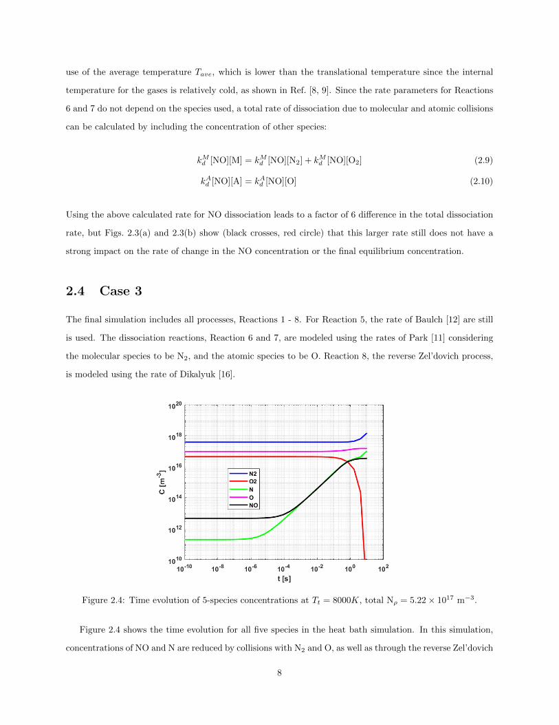
2.4 Case 3

The final simulation includes all processes, Reactions 1 - 8. For Reaction 5, the rate of Baulch [12] are still

is used. The dissociation reactions, Reaction 6 and 7, are modeled using the rates of Park [11] considering

the molecular species to be N2, and the atomic species to be O. Reaction 8, the reverse Zel’dovich process,

is modeled using the rate of Dikalyuk [16].

Figure 2.4: Time evolution of 5-species concentrations at Tt = 8000K, total Nρ = 5.22× 1017 m−3.

Figure 2.4 shows the time evolution for all five species in the heat bath simulation. In this simulation,

concentrations of NO and N are reduced by collisions with N2 and O, as well as through the reverse Zel’dovich

8

process. At t ≈ 1s, the concentrations of O and N2 begin to increase as more NO is destroyed by Reactions

6 - 8 than created by Reaction 5. The population of N still increases because the largest contributor to the

rate of change is Reaction 1, though the rate at which the concentration changes decreases for a short time

after t ≈ 1s. Still, there is no mechanism for O2 to be produced so the concentration tends to zero as the

simulation continues.

(a) Nitric oxide concentration time evolution at Tt = 15000K.

(b) Nitric oxide concentration evolution at Tt = 8000K.

Figure 2.5: Comparison of Case 1, 2, and 3 for two different temperatures.

To compare with previous simulations, Figs. 2.5(b) and 2.5(a) show the time evolution of the NO con-

centration for Case 1, 2, and 3. For Case 1 and 2, Reaction 5 uses the rates of Baulch [12]. For Case 2, the

dissociation mechanism is modeled using only Reaction 6 now with the rate of Andrienko [15]. The disso-

ciation rate is found by using a simplified QCT model that does not depend on the average temperature,

9

but rather the translational temperature, Tt. As a result, the rate of Andrienko [15] is higher than both

the rates of Cruden [14] and Park [11]. Still, the total rate of change of NO due to dissociation depends on

the concentration of NO, which remains relatively low for most of the time simulated. From Fig. 2.5(a) and

Fig. 2.5(b), the effect of increasing the temperature is once again illustrated by the time elapsed before dif-

ferences in NO concentration are observed. The peak NO concentration for each case occur now at t = 0.1s

at Tt = 15000K compared to t = 1s at Tt = 8000k.

For all of the reactions modeled, notable differences in species concentration occur after at least 100 ms

have elapsed. For the conditions simulated, the equilibrium time between collisions is:

τ =1

4d2refNρ

(πkT

u

0.5)(TrefT

1−ω) (2.11)

where dref is the reference diameter for a molecule of gas. Nρ is the number density of the gas, and ω is

the viscosity-temperature index of the gas. For the total number density considered, the minimum time

between collisions occurs with the lowest temperature, Tt = 8000k, and has a value of τ = 1.5 × 10−2 s.

Not all collisions have enough energy to dissociate NO or undergo an exchange reaction so there may be

many collisions before the NO molecule is destroyed. In the context of a CubeSat during reentry, by the

time such an event occurs, new gas particles have entered the bow-shock interaction zone and formed NO.

Because of this, the change in NO concentration past t = 0.1s where the slow reverse Zel’dovich reaction

begins to affect the NO concentration is not relevant to the short times at which particles reside in the shock

interaction zone.

10

Chapter 3

DSMC Numerical Methods

3.1 External Simulation Setup

The simulations of the CubeSat are performed using the DSMC Stochastic PArallel Rarefied-gas Time-

accurate Analyzer (SPARTA [18]) and Statistical Modeling in Low-Density Environment (SMILE [19]) codes.

Calculations are performed for external flow over the CubeSat for altitudes from 100 to 200 km because this

is the transitional regime of flow where measurements will be recorded by the UV and VIS spectrometers.

Measurements by the VIS spectrometer will take place starting at an altitude of 200km and will continue to

150 km. Below 150km, ultraviolet radiation will be recorded by two UV spectrometers. Based on trajectory

analyses, the velocity of the CubeSat for these altitudes will be approximately 7.55 km/s. The freestream

conditions used for the simulations are given in Tab. 3.1 and the list of reactions that are considered for the

external flow simulations are listed in Tab. 3.2 from Refs. [7] and [10]. The initial freestream mole fractions

at each altitude are shown in Tab. 3.3. For these simulations, the mole fractions for the major species are

from Jacchia [20] and the trace species are from the results of McCoy [21].

Table 3.1: Flow Simulation Parametersa.Freestream Parameter External Simulations

Altitude (km) 200 180 160 150 140 130 120 110 100Freestream Temperature (K) 1026 947 822 730.6 625 500 368 247 195λ(m) 250 170 66 40 22 10 3.4 0.77 0.13Knudsen Numberb 5000 3400 1320 800 442 201 69.6 15.5 2.6Mach 10.2 10.8 11.8 12.7 13.9 15.7 18.6 23.1 26.5

aA surface temperature of 300 K and a spacecraft velocity of 7,550 m/s were assumed.bKnudsen number for external flow simulations calculated using the edge length of the ram-face of thesimulated CubeSat.

The passive stability of the CubeSat will keep the ram face within an angle-of-attack of ± 2 degrees [23].

Since the flow is then symmetric across two planes, only a quarter of the domain needs to be simulated. The

simulated geometry of the 3U CubeSat is shown in Fig. 3.1(a). The baseline orientation of the CubeSat is

shown in Fig. 3.1(b) where the ram face is located at the origin; Fig. 3.1(c) shows the broadside orientation.

11

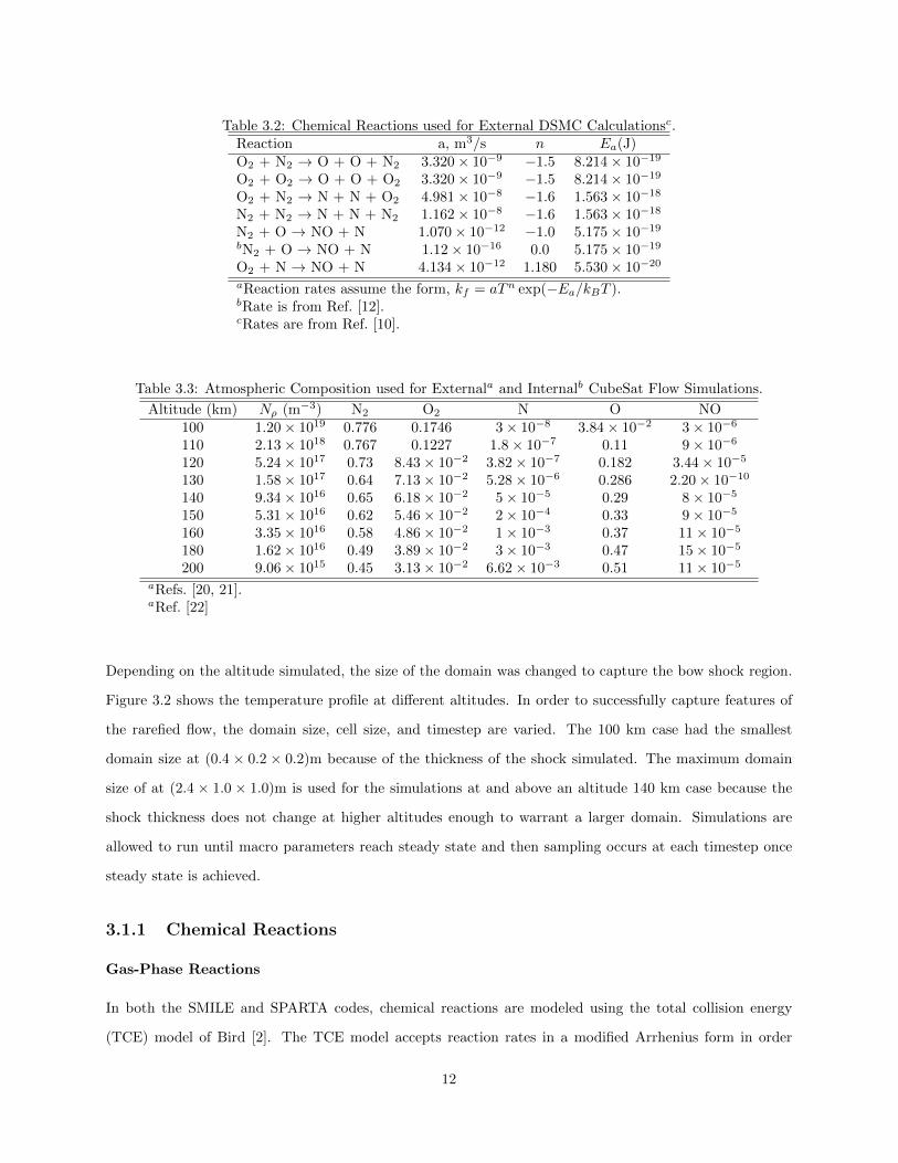
Table 3.2: Chemical Reactions used for External DSMC Calculationsc.Reaction a, m3/s n Ea(J)O2 + N2 → O + O + N2 3.320× 10−9 −1.5 8.214× 10−19

O2 + O2 → O + O + O2 3.320× 10−9 −1.5 8.214× 10−19

O2 + N2 → N + N + O2 4.981× 10−8 −1.6 1.563× 10−18

N2 + N2 → N + N + N2 1.162× 10−8 −1.6 1.563× 10−18

N2 + O → NO + N 1.070× 10−12 −1.0 5.175× 10−19

bN2 + O → NO + N 1.12× 10−16 0.0 5.175× 10−19

O2 + N → NO + N 4.134× 10−12 1.180 5.530× 10−20

aReaction rates assume the form, kf = aTn exp(−Ea/kBT ).bRate is from Ref. [12].cRates are from Ref. [10].

Table 3.3: Atmospheric Composition used for Externala and Internalb CubeSat Flow Simulations.

Altitude (km) Nρ (m−3) N2 O2 N O NO100 1.20× 1019 0.776 0.1746 3× 10−8 3.84× 10−2 3× 10−6

110 2.13× 1018 0.767 0.1227 1.8× 10−7 0.11 9× 10−6

120 5.24× 1017 0.73 8.43× 10−2 3.82× 10−7 0.182 3.44× 10−5

130 1.58× 1017 0.64 7.13× 10−2 5.28× 10−6 0.286 2.20× 10−10

140 9.34× 1016 0.65 6.18× 10−2 5× 10−5 0.29 8× 10−5

150 5.31× 1016 0.62 5.46× 10−2 2× 10−4 0.33 9× 10−5

160 3.35× 1016 0.58 4.86× 10−2 1× 10−3 0.37 11× 10−5

180 1.62× 1016 0.49 3.89× 10−2 3× 10−3 0.47 15× 10−5

200 9.06× 1015 0.45 3.13× 10−2 6.62× 10−3 0.51 11× 10−5

aRefs. [20, 21].aRef. [22]

Depending on the altitude simulated, the size of the domain was changed to capture the bow shock region.

Figure 3.2 shows the temperature profile at different altitudes. In order to successfully capture features of

the rarefied flow, the domain size, cell size, and timestep are varied. The 100 km case had the smallest

domain size at (0.4 × 0.2 × 0.2)m because of the thickness of the shock simulated. The maximum domain

size of at (2.4 × 1.0 × 1.0)m is used for the simulations at and above an altitude 140 km case because the

shock thickness does not change at higher altitudes enough to warrant a larger domain. Simulations are

allowed to run until macro parameters reach steady state and then sampling occurs at each timestep once

steady state is achieved.

3.1.1 Chemical Reactions

Gas-Phase Reactions

In both the SMILE and SPARTA codes, chemical reactions are modeled using the total collision energy

(TCE) model of Bird [2]. The TCE model accepts reaction rates in a modified Arrhenius form in order

12

(a) Simulated 3U CubeSat geometry.

(b) Baseline orientation of the CubeSat, ε = 0.33.

(c) Broadside orientation of the CubeSat, ε = 3.

Figure 3.1: Simulated CubeSat in quarter-domain at 100km with flow in the +X direction.

13

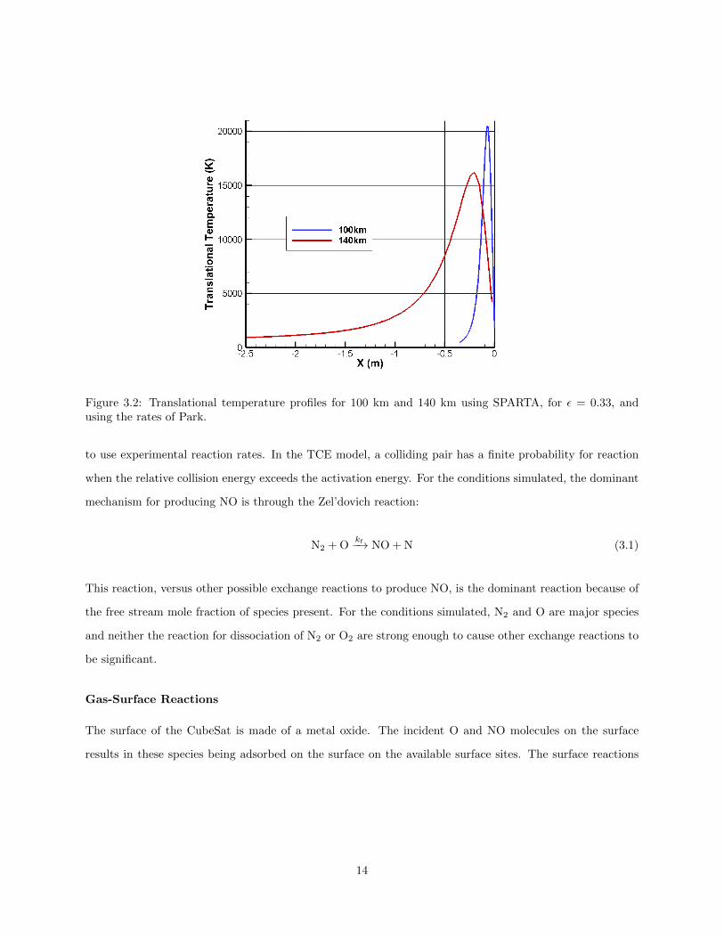
Figure 3.2: Translational temperature profiles for 100 km and 140 km using SPARTA, for ε = 0.33, andusing the rates of Park.

to use experimental reaction rates. In the TCE model, a colliding pair has a finite probability for reaction

when the relative collision energy exceeds the activation energy. For the conditions simulated, the dominant

mechanism for producing NO is through the Zel’dovich reaction:

N2 + Okf−→ NO + N (3.1)

This reaction, versus other possible exchange reactions to produce NO, is the dominant reaction because of

the free stream mole fraction of species present. For the conditions simulated, N2 and O are major species

and neither the reaction for dissociation of N2 or O2 are strong enough to cause other exchange reactions to

be significant.

Gas-Surface Reactions

The surface of the CubeSat is made of a metal oxide. The incident O and NO molecules on the surface

results in these species being adsorbed on the surface on the available surface sites. The surface reactions

14

used in this work for O and NO species are summarized as follows [7, 8]:

NO + S ←→ NOS (3.2)

O + S ←→ OS (3.3)

NOS + Okf3.4−−−→ NO∗

2 + S (3.4)

NO + OS

kf3.5−−−→ NO∗2 + S (3.5)

NOS + OS

kf3.6−−−→ NO∗2 + S, (3.6)

where S represents a surface site on the metal oxide surface. The adsorption-desorption reactions numbered

3.2 and 3.3 are reversible. Reactions 3.4 and 3.5 follow an Eley-Rideal mechanism where one of the species

is in the gas phase and the other is adsorbed on the surface. Reaction 3.6 follows a Langmuir-Hinshelwood

mechanism where all the reactants are adsorbed on the surface and can diffuse between surface sites to form

products [24].

The forward (adsorption) rate for Reactions 3.2 and 3.3 is determined from the sticking probability of NO

and O species on the surface. Their backward (desorption) rate is, however, determined based on their heat

of desorption [7]. Since the heat of adsorption for O is about five times smaller than that of NO, O atoms

have a very low residence time on the surface making Reaction 3.4 the most dominant for producing NO∗2.

A value of 16 kcal/mol for the heat of adsorption of O in the surface is used in this work. At steady state,

surface coverage of NO reaches a constant value with a constant O and NO flux incident on the surface.

Since the reaction rates for gas-surface reactions are much smaller compared to that of gas-phase reactions,

the gas-surface processes are assumed to be decoupled from the gas-phase calculations and use O and NO

surface fluxes obtained from the DSMC gas phase calculations.

3.1.2 Radiation Calculations

Visible Radiation

The primary source of visible radiation around the CubeSat is considered to be NO∗2 [7, 25]. Molecules of

NO∗2 are formed on the surface of the CubeSat as per the surface chemical reactions 3.2-3.6. The tangent

slab approximation model is used for estimating visible radiation due to NO∗2. This model is used in Ref. [7]

where radiation intensity is given by,

I =σf3.4nNOx

fO + σf3.5nOxfNO

2, (3.7)

15

where fO and fNO are the fluxes of O and NO on the surface, nNOx and nOx are the surface number density

(molecules/m2) of NO and O adsorbed on the surface, and σf4 and σf5 are the cross sections of surface

reactions 3.4 and 3.5. The spacecraft glow calculations are performed using the steady state DSMC solutions

for the CubeSat geometry. The radiance due to NO∗2 produced on the surface will be discussed in Section 5.

UV Radiation

The primary source of ultraviolet radiation is expected to be from NO (γ)-band radiation [21, 26]. NO(γ)-

band radiation is produced by the A2Σ+ → X2∏

transition, so in order to estimate the radiative intensity,

the population density of NO(A) state must be determined. At these altitudes, there are insufficient collision

to form a Boltzmann distribution and therefore the mechanisms for populating the excited electronic states

must be specified. In this work, only heavy-body collisional processes are considered as the degree of

ionization is assumed to be very low. Future work will study this assumption by including excitation and

deexcitation processes due to electron impact. The specific processes by which NO may be excited and

deexcited are given as:

NO(i) + WK(i,j)−−−−→ NO(j) + W (3.8)

N + O + WKWi−−−→ NO(i) + W (3.9)

NO(i)A(i,j)−−−−→ NO(j) + hν (3.10)

where K(i, j) for Reaction 3.8 is the neutral impact excitation rate coefficient for i < j and deexcitation rate

coefficient if i > j. In Reaction 3.9, Kwi is the heavy-body recombination rate coefficient while Kiw is the

rate coefficient due to heavy body dissociation caused by species W, where W is another heavy particle. The

last process considered for excitation and deexcitation is Reaction 3.10, where A(i, j) is the spontaneous

emission rate coefficient from electronic level i to j. To determine the number of NO molecules in each

excited state, the reactions form a system of master equations given by Park[1] as:

∂Ni∂t

=

m∑j=1

K(j, i)NjNW +

m∑j=1

A(j, i)Nj +KWiNONNNW

−m∑j=1

K(i, j)NiNW −m∑j=1

A(i, j)Ni −KiWNWNi (3.11)

When the rate of change of Ni is very small, the condition is known as the quasi-steady-state (QSS) condition,

and the left hand side is equated to zero. The simplification of Eq. 3.11 allows for the excitation and

deexcitation quantities to be put into matrix form so that the system of equations can be solved for the

16

vector N, the number density of the ith electronic level:

MN = C (3.12)

The diagonal elements of M are:

M(i, i) =

m∑j=1

(K(i, j) +

A(i, j)

NW

)+KiW (3.13)

and the off-diagonal elements of M are:

M(i, j) = −K(j, i)− A(j, i)

NW(3.14)

The elements of vector C are:

C(i) = KWiNNNO (3.15)

As a simplification, the conservation equation, Eq. 3.16 may be substituted in for the i = 1 level of the

QSS equation:

m∑j=1

Ni = NNO (3.16)

which corresponds to matrix values of M(1, j) = 1 and C(1) = NNO. The vector N is determined by

inverting the m×m matrix M and multiplying with the column vector C.

17

Chapter 4

Direct Simulation Monte CarloResults

4.1 External Flowfield Sensitivity Analysis

To quantify the variance of predicted NO formation as the CubeSat descends through Earth’s atmosphere,

external simulations are performed with several different parameters. Table 4.1 summarizes the DSMC

numerical parameters considered for the different altitudes and cases considered, and the figures shown are

at an altitude of 120km. The order of the sensitivity analysis is chosen in ascending order of its effect on

the mole fraction of NO.

Table 4.1: Case Definitions for Sensitivity Analysis of External Simulationsa.

Case (#) DSMC Code ε Zel’dovich Rate σ1(a) SPARTA 0.33 Park 1.01(b) SPARTA 0.33 Park 0.92(a) SPARTA 0.33 Baulch 1.02(b) SMILE 0.33 Baulch 1.0

3 SPARTA 3.0 Baulch 1.0aCases shown are for an altitude of 120 km.

4.2 Surface Accommodation Coefficient

Figure 4.1(a) shows the translational and internal temperatures predicted for both altitudes along the stag-

nation line in the shock region using SPARTA. The ram face of the CubeSat is located at the origin as seen in

Figs. 3.1(b) and 3.1(c). For high altitudes where N2 is the dominant species, the rarefaction results in a large

mean time between collisions which results in a low chance for particles to exchange energy with internal

modes, which is similar to the result observed by Dogra et al [8]. The vibrational and rotational temperature

do not significantly change for σ = 0.9 when compared to σ = 1.0. The translational temperature varies

significantly for different values of σ because of the difference in velocities for reflected particles. When

σ = 1.0, particles are emitted from the surface with a most probable speed equal to the surface temperature

of 300 K. When σ = 0.9, 10% of incident particles retain their energy after striking the surface. The small

18

fraction of these highly energetic reflected particles then changes the average kinetic energy of the particles

in each cell. Since the flow is highly directional for both altitudes, the translational temperature is elevated

significantly along the stagnation line. Since the internal temperatures do not change significantly when

changing other simulation parameters, they are not shown in the remaining figures. Presented in Fig. 4.1(b)

is the number density profile along the stagnation line for Cases 1(a) and 1(b) and it can be seen the that the

mole fraction does not change significantly along the stagnation line. The sensitivity of radiation produced

in the UV and VIS regime to thermal accommodation coefficient will be investigated in future work.

4.3 Chemical Reaction Rates

Two different reaction rates are used to assess NO production sensitivity to different rates for the Zel’dovich

reaction. The rates used come from the set of Park [10] and Baulch[12], and were used in the earlier

works [8, 10]. The reaction rates have the same activation energies as can be seen in Tab. 3.2, but have

a somewhat different temperature dependencies as seen in Fig 4.2. At higher temperatures the forward

reaction rate coefficient, kf , is higher for the rates of Baulch [12] than the rates of Park [10]. Even though

the temperature remains nearly the same as seen in Fig. 4.3(a), Fig. 4.3(b) shows the change in NO mole

fraction due to variation of the chemical reaction rate. When the rate given by Park [10] is used, more NO

is produced in the shock region than when using the rates of Baulch [12]. The mole fraction of NO increases

in the region close to the body (near the origin) when using the rates of Park [10] because the rate is higher

for the gas temperature close to the body where most collisions occur. The concentration of the free stream

NO is nearly recovered upstream of the shock, where particles can no longer diffuse and the reactions are

not as likely.

4.4 CubeSat Orientation

To investigate the flowfield dependence on CubeSat orientation, simulations are performed with the CubeSat

oriented 90 degrees to its current flow orientation using both SMILE and SPARTA. Figure 3.1 shows the

two different CubeSat orientations used in this analysis, and the corresponding aspect ratio:

ε =lnormalledge

(4.1)

where lnormal and ledge are the longest edge length of the face normal and parallel to the flow respectively.

It can be seen from Fig. 4.4 that by altering the orientation of the CubeSat, the size of the diffuse shock

19

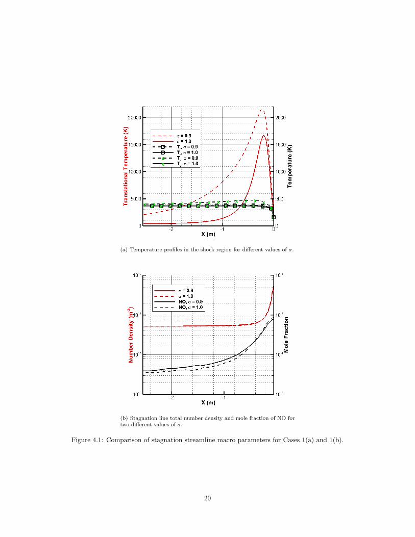
(a) Temperature profiles in the shock region for different values of σ.

(b) Stagnation line total number density and mole fraction of NO fortwo different values of σ.

Figure 4.1: Comparison of stagnation streamline macro parameters for Cases 1(a) and 1(b).

20

Figure 4.2: Forward rate coefficient change with temperature for the Zel’dovich reaction from the set of Parkand Baulch.

interaction region changes. The increase in NO production is due to the larger area that freestream particles

can strike. Increasing the number of particles that strike the surface, increases the number of reflections.

The subsequent increase in gas-gas collisions broadens the shock as shown in Fig. 4.4(a), and the increase

in number of collisions promotes the formation of NO which can be seen in Fig. 4.4(b).

4.5 Model Differences

Although both the SMILE and SPARTA codes use the TCE model, their implementations differ. For

one, in the SPARTA code, the TCE model uses an effective internal degree of freedom equal to one as

demonstrated by Bird [2]. Figure 4.5 shows the difference in probability for the Zel’dovich reaction to occur

after being considered for reaction and it can be seen that for each colliding pair with sufficient collision

energy, the expression used by the SPARTA code results in a higher probability for the reaction to take

place. Additionally, in the post-collision relaxation calculation, SPARTA uses a constant vibrational degree

of freedom equal to two, whereas the SMILE code uses a temperature dependent vibrational degree of

freedom.

The model differences result in slightly different shock thicknesses. SPARTA predicts shocks that are

slightly more diffuse as shown in Fig. 4.6(a). The large increase in predicted NO number seen in Fig. 4.6(b)

arises from the difference in probability for a reaction to occur between the SPARTA and SMILE codes,

which comes from the different effective internal degrees of freedom and temperatures employed.

21

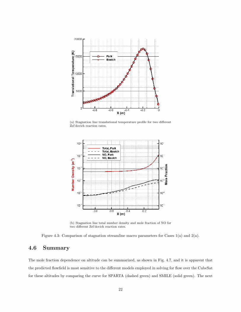
(a) Stagnation line translational temperature profile for two differentZel’dovich reaction rates.

(b) Stagnation line total number density and mole fraction of NO fortwo different Zel’dovich reaction rates.

Figure 4.3: Comparison of stagnation streamline macro parameters for Cases 1(a) and 2(a).

4.6 Summary

The mole fraction dependence on altitude can be summarized, as shown in Fig. 4.7, and it is apparent that

the predicted flowfield is most sensitive to the different models employed in solving for flow over the CubeSat

for these altitudes by comparing the curve for SPARTA (dashed green) and SMILE (solid green). The next

22

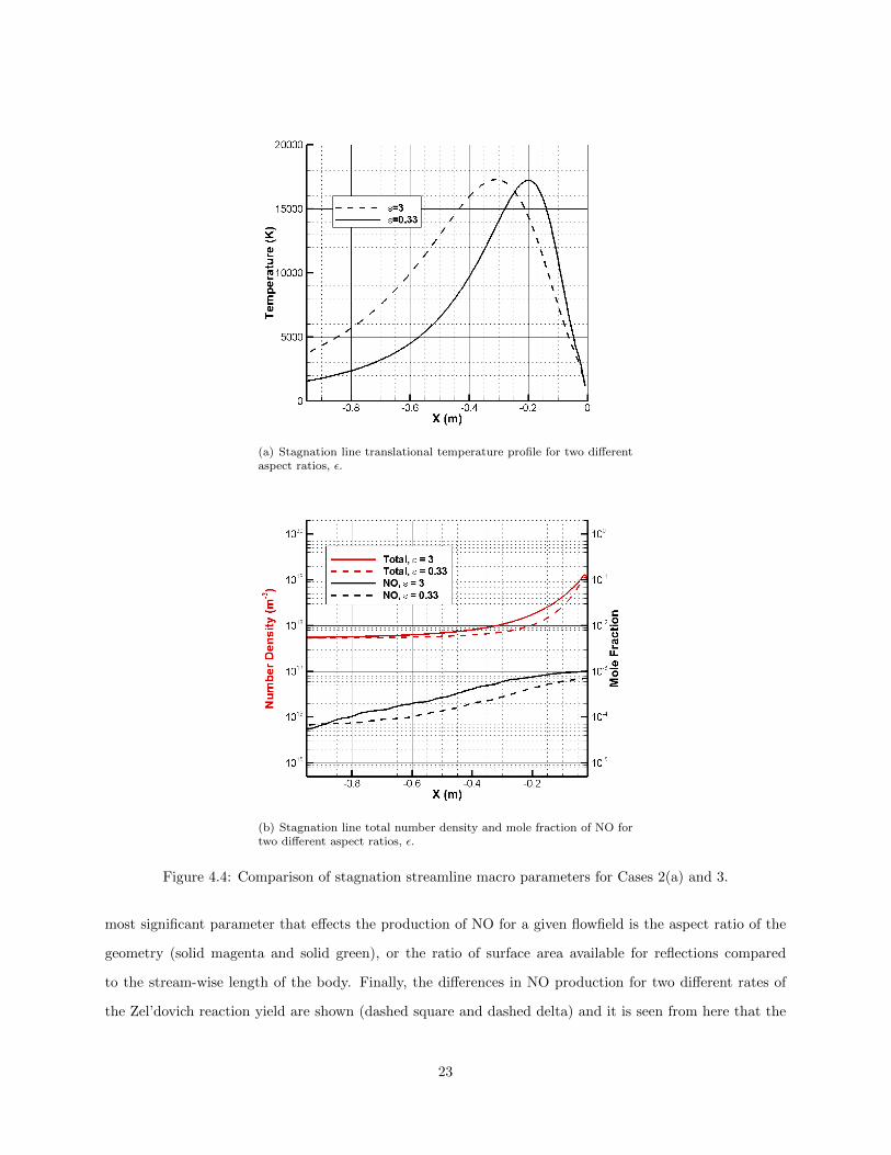
(a) Stagnation line translational temperature profile for two differentaspect ratios, ε.

(b) Stagnation line total number density and mole fraction of NO fortwo different aspect ratios, ε.

Figure 4.4: Comparison of stagnation streamline macro parameters for Cases 2(a) and 3.

most significant parameter that effects the production of NO for a given flowfield is the aspect ratio of the

geometry (solid magenta and solid green), or the ratio of surface area available for reflections compared

to the stream-wise length of the body. Finally, the differences in NO production for two different rates of

the Zel’dovich reaction yield are shown (dashed square and dashed delta) and it is seen from here that the

23

Figure 4.5: Probability for Zel’dovich exchange reaction of Park to take place using SPARTA and SMILE.

differences vary across the range of altitudes. As the CubeSat descends to lower altitudes, the shock region

becomes thinner and the peak temperature in the shock is raised when the speed is maintained. For higher

temperatures, the reaction rate coefficient of Park [10] will become larger, leading to greater differences in

predicted NO mole fractions. The mole fraction of produced NO depends on N2 and O, the reactants of the

first Zel’dovich reaction (Reaction 3.1). Owing to the low reaction-rate of N2 dissociation, nearly all of N2

in the domain is available for Reaction 3.1. On the other hand, availability of O in the domain is affected

by the mole fraction of O in free stream and the dissociation of free stream O2 in the shock region. The free

stream mole fractions of O and O2 are decreasing and increasing respectively with decreasing altitude as

shown in Tab. 3.3. Because of this contrasting trend, although a steady increase of the mole fraction of NO

is observed with decrease in altitude for our range of 100 to 200 km, a general comment cannot be made for

NO mole fractions produced in the shock regions of the flow at other altitudes. Figure 5.1 shows the surface

flux of particles striking the stagnation point of the CubeSat for different altitudes, and it is more evident

from these curves that the concentration of NO is increasing, but is never higher than that of O. Figure 5.1

also shows that at higher altitudes where formation of NO is less likely, sensitivity to modeling parameters

also becomes weaker.

24

(a) Stagnation line translational temperature profile for two differentDSMC codes.

(b) Stagnation line total number density and mole fraction of NO fortwo different DSMC codes.

Figure 4.6: Comparison of stagnation streamline macro parameters for Cases 2(a) and 2(b).

25

Figure 4.7: Stagnation point total number density of all species with change in altitude (red). Stagnationpoint mole fractions for NO is shown for different chemical reaction rates (symbols), DSMC code (line style),and different CubeSat orientation (color).

26

Chapter 5

Radiation Estimates

5.1 Visible Radiation

A spectrometer onboard CubeSat will be dedicated to the radiation in the spectral range from 500 to 800

nm. As mentioned before, NO∗2 is the prime source of emission spectra in the visible spectral range. and

since it is a tri-atomic molecule, its spectra is broad ranging from 500 to 800 nm [27, 28]. Surface flux data

using the SPARTA code, shown in Fig. 5.1, is used to calculate the radiance (in Rayleighs) for NO∗2 given

by Eq. 3.7. In Fig. 5.2(a), the radiance is slightly higher for the ε = 3.0 orientation of CubeSat compared

to ε = 0.33 orientation because of the larger NO flux on the surface, as discussed in Fig. 5.1. Although the

gas phase calculations using the chemistry model of Park [10] generate more NO compared to Baulch [12],

the NO mole fraction near the surface does not show a significant difference, as was shown in Fig. 4.7. This

is reflected in Fig. 5.2(a) where the radiance due to the Park and Baulch rates for ε = 0.33 are nearly the

same. Figure 5.2(a) also compares the NO∗2 radiance prediction from Gimelshein et al.[7] for a cylindrical

geometry of the Atmospheric Explorer (AE) (diameter= 2 m). Since our geometry is more than one order

of magnitude smaller in comparison, the radiance for the CubeSat is about an order of magnitude smaller

than that of AE, which can be seen in Fig. 5.2(b).

5.2 UV Radiation

Onboard the CubeSat, two spectrometers will measure UV radiation that is produced from gas-phase

molecules undergoing electronic transitions in the wavelength range from 205 to 255 nm. Figure 5.3 shows

the NO(γ) and NO(β) band emission profiles. At the altitude of 100 km, the NO(β)-band emission is the

highest it will be for the altitudes simulated, and is still more than one magnitude lower in intensity than

the peak emission from NO(γ)-band emission, so the peak emission of NO(γ)-band is the most important

in this work. Similar to Fig. 4.7, Fig. 5.4 demonstrates the sensitivity of NO (γ)-band radiation to different

modeling parameters. Inspection of the plot shows that the highest predicted radiance at each altitude

27

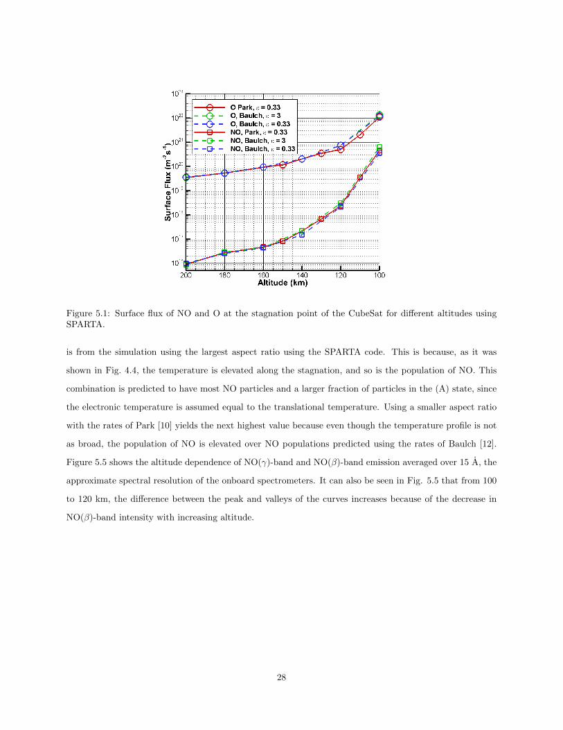
Figure 5.1: Surface flux of NO and O at the stagnation point of the CubeSat for different altitudes usingSPARTA.

is from the simulation using the largest aspect ratio using the SPARTA code. This is because, as it was

shown in Fig. 4.4, the temperature is elevated along the stagnation, and so is the population of NO. This

combination is predicted to have most NO particles and a larger fraction of particles in the (A) state, since

the electronic temperature is assumed equal to the translational temperature. Using a smaller aspect ratio

with the rates of Park [10] yields the next highest value because even though the temperature profile is not

as broad, the population of NO is elevated over NO populations predicted using the rates of Baulch [12].

Figure 5.5 shows the altitude dependence of NO(γ)-band and NO(β)-band emission averaged over 15 A, the

approximate spectral resolution of the onboard spectrometers. It can also be seen in Fig. 5.5 that from 100

to 120 km, the difference between the peak and valleys of the curves increases because of the decrease in

NO(β)-band intensity with increasing altitude.

28

(a) Radiance of NO∗2 emission at different altitudes using rates of Park

and Baulch.

(b) Stagnation line number density for AE and SASSI2 simulations at140 km using rates of Baulch.

Figure 5.2: Comparison of NO∗2 emission estimates between AE and SASSI2 simulations using SPARTA.

29

Figure 5.3: Line-by-line spectral radiance of NO(γ)-band and NO(γ)-band emission at 100km using SPARTA,rates of Baulch, and an aspect ratio of ε = 0.33. ∆λ = 6.3× 10−3A.

Figure 5.4: Difference in mean radiance of NO (γ)-band emission spectrum over 205 to 255 nm wavelengthrange, with change in chemical reaction set, DSMC code, and CubeSat aspect ratio ε. A pass-band filter for230 ± 25nm is used from Levin.

30

Figure 5.5: NO(γ) and NO(β)-band emission profiles in the 205 to 255 nm wavelength range across 100,120, and 140km, using SPARTA, rates of Baulch, and an aspect ratio of ε = 0.33.

31

Chapter 6

Conclusions

Numerical calculations have been performed to determine the sensitivity of previous work to dissociation

and reverse exchange reactions for NO. It has been found that dissociation and reverse exchange mechanisms

have negligible effect on the NO produced during the time the particle resides in the bow shock. DSMC

flowfield solutions for altitudes from 100 to 200 km have been performed using the SPARTA and SMILE

codes. It has been determined that the calculated probability for the first Zel’dovich reaction to occur by

SMILE or SMART has the greatest impact on the prediction of NO formation in the diffuse shock region

of the 3U CubeSat. Estimates of NO formation have been used to determine the amount of NO2 that

will be present due to surface reactions, and the tangent slab approximation has been used to estimate the

spacecraft glow radiance in the visible range. After selecting mechanisms for electronic state excitation,

calculations using NEQAIR have shown the intensity of radiation that can be expected from NO and it has

been determined that the NO(γ)-band radiation is the most significant band of ultraviolet radiation for this

mission. A comparison with simulations performed at similar altitudes for previous missions has shown that

the radiation intensity is strongly dependent on the size of the geometry, which directly influences the size

of the shock interaction region.

32

References

[1] Park, C., “Nonequilibrium Hypersonic Aerothermodynamics,” 1989.

[2] Bird, G., “Molecular Gas Dynamics and the Direct Simulation Monte Carlo of Gas Flows,” Clarendon,Oxford , Vol. 508, 1994, pp. 128.

[3] Park, C., “Nonequilibrium Air Radiation (NEQAIR) Program [Microform]: User’s Manual/Chul Park,”NASA, TM-86707 , 1985.

[4] Cauchon, D. L., “Radiative Heating Results from the FIRE II Flight Experiment at a Reentry Velocityof 11.4 Kilometers per Second,” NASA TM X-1402 , Vol. 6, 1967.

[5] Levin, D., Candler, G., Collins, R., Erdman, P., Zipf, E., Espy, P., and Howlett, C., “Comparison ofTheory with Experiment for the Bow Shock Ultraviolet Rocket Flight.” Journal of Thermophysics andHeat Transfer , Vol. 7, No. 1, 1993, pp. 30–36.

[6] Levin, D. A., Candler, G. V., Collins, R. J., Erdman, P. W., Zipf, E. C., and Howlett, L. C., “Examina-tion of Theory for Bow Shock Ultraviolet Rocket Experiments-I,” Journal of Thermophysics and Heattransfer , Vol. 8, No. 3, 1994, pp. 447–452.

[7] Gimelshein, S., Levin, D., and Collins, R., “Modeling of Glow Radiation in the Rarefied Flow About anOrbiting Spacecraft,” Journal of Thermophysics and Heat transfer , Vol. 14, No. 4, 2000, pp. 471–479.

[8] Dogra, V. K., Collins, R. J., and Levin, D. A., “Modeling of Spacecraft Rarefied Environments Usinga Proposed Surface Model,” AIAA Journal , Vol. 37, No. 4, 1999, pp. 443–452.

[9] Morgan, J., Nuwal, N., Williams, J., Putnam, Z. R., Levin, D., Pikus, A., Berger, A., and Alexeenko,A., “Prediction of Flight Measurements of High-Enthalpy Nonequilibrium Flow from a CubeSat-ClassAtmospheric Probe,” AIAA Aerospace Sciences Meeting , Vol. 812, 2018.

[10] Li, Z., Sohn, I., and Levin, D. A., “Modeling of Nitrogen Monoxide Formation and Radiation in Nonequi-librium Hypersonic Flows,” Journal of Thermophysics and Heat Transfer , Vol. 28, No. 3, 2014, pp. 365–380.

[11] Park, C., “Review of Chemical-Kinetic Problems of Future NASA Missions. I-Earth Entries,” Journalof Thermophysics and Heat transfer , Vol. 7, No. 3, 1993, pp. 385–398.

[12] Baulch, D. L., “Evaluated Kinetic Data for High Temperature Reactions,” Cleveland, CRC Press [1972-,1972.

[13] Luo, H., Kulakhmetov, M., and Alexeenko, A., “Ab initio state-specific N 2 + O Dissociation andExchange Modeling for Molecular Simulations,” The Journal of Chemical Physics, Vol. 146, No. 146,2017, pp. 24309–24310.

[14] Cruden, B. A. and Brandis, A. M., “Measurement of Radiative Non-equilibrium for Air Shocks Between7-9 km/s,” 47th AIAA Thermophysics Conference, 2017, p. 4535.

[15] Andrienko, D. and Boyd, I. D., “State-resolved Characterization of Nitric Oxide Formation in ShockFlows,” 2018 AIAA Aerospace Sciences Meeting , 2018, p. 1233.

33

[16] Dikalyuk, A., Kozlov, P., Romanenko, Y., Shatalov, O., and Surzhikov, S., “Nonequilibrium spectralradiation behind the shock waves in Martian and Earth atmospheres,” 44th AIAA ThermophysicsConference, 2013, p. 2505.

[17] Bose, D. and Candler, G. V., “Thermal Rate Constants of the N2+ O→ NO+ N Reaction using abinitio 3A” and 3A’ Potential Energy Surfaces,” The Journal of chemical physics, Vol. 104, No. 8, 1996,pp. 2825–2833.

[18] Gallis, M. A., Torczynski, J. R., Plimpton, S. J., Rader, D. J., and Koehler, T., “Direct simulationMonte Carlo: The quest for speed,” AIP Conference Proceedings, Vol. 1628, 2014, pp. 27–36.

[19] Ivanov, M., Kashkovsky, A., Gimelshein, S., Markelov, G., Alexeenko, A., Bondar, Y. A., Zhukova, G.,Nikiforov, S., and Vaschenkov, P., “SMILE System for 2D/3D DSMC Computations,” Proceedings of25th International Symposium on Rarefied Gas Dynamics, St. Petersburg, Russia, 2006, pp. 21–28.

[20] Jacchia, L. G., “Thermospheric Temperature, Density, and Composition: New Models,” SAO SpecialReport , Vol. 375, 1977.

[21] McCoy, R. P., “Thermospheric Odd Nitrogen: 1. NO, N (4 S), and O (3P) Densities from RocketMeasurements of the NO δ and γ Bands and the O2 Herzberg I Bands,” Journal of Geophysical Research:Space Physics, Vol. 88, No. A4, 1983, pp. 3197–3205.

[22] Jelezniak, M. and Jelezniak, I., “CHEMKED 3.3,” 2013.

[23] Zuiker, N. J., Williams, J., Putnam, Z. R., Levin, D. A., Ghosh, A., Goggin, M., and Alexeenko, A.,“Design of a CubeSat Mission to Investigate High-Enthalpy Nonequilibrium Flow Chemistry,” 2018AIAA Aerospace Sciences Meeting , 2018, p. 1936.

[24] Gasser, R. P. H. and Ehrlich, G., “An Introduction to Chemisorption and Catalysis by Metals,” PhysicsToday , Vol. 40, 1987, pp. 128.

[25] Murad, E., “The Shuttle Glow Phenomenon,” Annual Review of Physical Chemistry , Vol. 49, No. 1,1998, pp. 73–98.

[26] Erdman, P. W., Zipf, E. C., Espy, P., Howlett, L. C., Levin, D. A., Collins, R. J., and Candler, G. V.,“Measurements of Ultraviolet Radiation from a 5-km/s Bow Shock,” Journal of Thermophysics andHeat Transfer , Vol. 8, No. 3, 1994, pp. 441–446.

[27] Karipides, D. P., Boyd, I. D., and Caledonia, G. E., “Detailed Simulation of Surface Chemistry Leadingto Spacecraft Glow,” Journal of Spacecraft and Rockets, Vol. 36, No. 4, 1999, pp. 566–572.

[28] Kenner, R. and Ogryzlo, E., “Orange Chemiluminescence from NO2,” The Journal of chemical physics,Vol. 80, No. 1, 1984, pp. 1–6.

34