UNIVERSITY OF OULU P .O. Box 8000 F I -90014 UNIVERSITY OF OULU FINLAND

A C T A U N I V E R S I T A T I S O U L U E N S I S

University Lecturer Tuomo Glumoff

University Lecturer Santeri Palviainen

Postdoctoral research fellow Sanna Taskila

Professor Olli Vuolteenaho

University Lecturer Veli-Matti Ulvinen

Planning Director Pertti Tikkanen

Professor Jari Juga

University Lecturer Anu Soikkeli

Professor Olli Vuolteenaho

Publications Editor Kirsti Nurkkala

ISBN 978-952-62-1775-8 (Paperback)ISBN 978-952-62-1776-5 (PDF)ISSN 0355-3213 (Print)ISSN 1796-2226 (Online)

U N I V E R S I TAT I S O U L U E N S I SACTAC

TECHNICA

U N I V E R S I TAT I S O U L U E N S I SACTAC

TECHNICA

OULU 2018

C 643

Ekaterina Kaparulina

EURASIAN ARCTIC ICE SHEETS IN TRANSITIONS– CONSEQUENCES FOR CLIMATE, ENVIRONMENT AND OCEAN CIRCULATION

UNIVERSITY OF OULU GRADUATE SCHOOL;UNIVERSITY OF OULU,FACULTY OF TECHNOLOGY,OULU MINING SCHOOL

C 643

AC

TAE

katerina Kap

arulina

C643etukansi.kesken.fm Page 1 Friday, December 1, 2017 2:58 PM

ACTA UNIVERS ITAT I S OULUENS I SC Te c h n i c a 6 4 3

EKATERINA KAPARULINA

EURASIAN ARCTIC ICE SHEETS IN TRANSITIONS – CONSEQUENCES FOR CLIMATE, ENVIRONMENT AND OCEAN CIRCULATION

Academic dissertation to be presented with the assent ofthe Doctoral Training Committee of Technology andNatural Sciences of the University of Oulu for publicdefence in Auditorium IT116, Linnanmaa, on 26 January2018, at 12 noon

UNIVERSITY OF OULU, OULU 2018

Copyright © 2018Acta Univ. Oul. C 643, 2018

Supervised byProfessor Kari StrandProfessor Juha Pekka Lunkka

Reviewed byDoctor Anu KaakinenDoctor Matt O’Regan

ISBN 978-952-62-1775-8 (Paperback)ISBN 978-952-62-1776-5 (PDF)

ISSN 0355-3213 (Printed)ISSN 1796-2226 (Online)

Cover DesignRaimo Ahonen

JUVENES PRINTTAMPERE 2018

OpponentProfessor Philip Gibbard

Kaparulina, Ekaterina, Eurasian Arctic ice sheets in transitions – consequences forclimate, environment and ocean circulation. University of Oulu Graduate School; University of Oulu, Faculty of Technology, Oulu MiningSchoolActa Univ. Oul. C 643, 2018University of Oulu, P.O. Box 8000, FI-90014 University of Oulu, Finland

Abstract

In this Ph.D. thesis sediment cores from the central Arctic Ocean, southwestern Barents Sea andsediment exposures from the Kola Peninsula were investigated in order to reveal interactionsbetween the late middle Pleistocene and late Pleistocene Arctic ice sheets, between Marine IsotopeStages 6 and 1 (MIS 6 and MIS 1). One of the main objectives of this work is to establishprovenance areas for the sediments studied in the central Arctic, the southwestern (SW) BarentsSea and the Kola Peninsula, their transport mechanisms and through that their relationship toglaciations in the Arctic and to development in the Kola Peninsula during the late middle and latePleistocene. Mineralogical and geochemical data from the core 96/12-1pc on the LomonosovRidge, central Arctic Ocean was studied to evaluate ice transport from circum-Arctic ice sheetsand variability in sediment drainage systems associated with their decay. SW Barents Seasediments contain important information on Late Glacial and Holocene sediment provenancecharacteristics in relation to ice flow patterns and ice rafting from different regional sectors. Thestudied SW Barents Sea sediment cores show that sediments were most likely derived from acombination of far-field Fennoscandian sources, local subcropping Mesozoic strata below theseafloor and sea ice transport. The investigation carried out on the Kola Peninsula indicates thatthe Eemian (MIS 5e) marine environment in the White Sea Basin and onshore coastal areasgradually changed into a glaciolacustrine environment during MIS 5d to MIS 5a. Subsequently,the Scandinavian Ice Sheet (SIS) covered the Kola Peninsula, most probably during MIS 4. Thefinal deglaciation of the SIS on the Kola Peninsula took place, however, during the lateWeichselian (MIS 2) between 16–12 ka.

Keywords: Arctic, Barents Sea, clay minerals, climate, glaciation, heavy minerals,Holocene, icebergs, Kola Peninsula, Late Glacial, late Pleistocene, Lomonosov Ridge,sea ice, Weichselian

Kaparulina, Ekaterina, Euraasian Arktisten jääkenttien muutokset – vaikutuksetilmastöön, ympäristöön ja merivirtoihin. Oulun yliopiston tutkijakoulu; Oulun yliopisto, Teknillinen tiedekunta, Oulu Mining SchoolActa Univ. Oul. C 643, 2018Oulun yliopisto, PL 8000, 90014 Oulun yliopisto

Tiivistelmä

Tässä väitöstutkimuksessa tutkittiin sedimenttikairanäytteitä keskeiseltä Jäämereltä ja Lounais-Barentsinmereltä sekä tarkasteltiin sedimenttiseurantoja Kuolan niemimaalla tarkoituksena sel-vittää myöhäisen keskipleistoseeni- ja myöhäispleistoseeniajan Arktisten jääkenttien keskinäisetvuorovaikutukset erityisesti merellisten isotooppivaiheiden 6 ja 1 (MIS 6 ja MIS 1) välillä.Tämän työn yhtenä päätavoitteena on määritellä sedimenttien lähdealueet keskeisellä Arktiksel-la, lounaisella Barentsinmerellä ja Kuolan niemimaalla, sedimenttien kuljetusmekanismit ja näi-den perusteella riippuvuudet Arktisiin jäätiköihin ja Kuolan niemimaalla tapahtuneeseen myö-häiskeski- ja myöhäispleistoseenin kehitykseen. Mineraloginen ja geokemiallinen tieto Lomo-nosovin harjanteen kairauksesta 96/12-1pc, keskeisellä Jäämerellä on perusta arvioitaessa jää-kuljetusmekanismeja ympäröiviltä sirkum-Arktisilta jäätiköiltä ja arvioitaessa valuma-alueidenosuutta suhteessa näiden jäätiköiden häviämiseen. Lounaisen Barentsinmeren sedimentit sisältä-vät tärkeätä tietoja viimeisen jäätiköitymisen loppuvaiheen ja holoseeni-ajan sedimenttien lähde-alueista ja suhteista jäävirtauksiin ja jääkuljetukseen eri aluesektoreilta. Tutkitut Lounais-Barent-sinmeren sedimentit osoittavat, että sedimentit olivat todennäköisimmin peräisin suhteellisenkaukaisilta Fennoscandian lähdealueilta, paikallisista mesotsoosista merenpohjan kerrostumistaja merijään kuljettamasta materiaalista. Kuolan niemimaalla tehty tutkimus osoittaa, että Eem-kauden (MIS 5e) meriympäristö Vienanmeren altaassa ja rannikkoalueilla vähitellen muuttuiglaciolakustriseksi ympäristöksi MIS 5d:n ja MIS 5a:n välisenä aikana. Sen jälkeen Skandinavi-an jääkenttä (SIS) peitti Kuolan niemimaan, todennäköisimmin koko MIS:n 4 ajanjakson. SIS:nlopullinen deglasiaatio alkoi Kuolan niemimaalla kuitenkin myöhäisen Veiksel-jääkauden (MIS2) aikana noin 16–12 ka sitten.

Asiasanat: Arktis, Barentsinmeri, holoseeni, ilmasto, jäätiköityminen, jäävuoret,Kuolan niemimaa, Lomonosovin harjanne, merijää, myöhäisglasiaalinen,myöhäispleistoseeni, raskasmineraalit, savimineraalit, Veiksel

7

Acknowledgements

This study is a part of the “Rapid environmental changes in the Eurasian Arctic –

Lessons from the past to the future” (REAL) research project carried out

cooperatively by the Thule Institute and the Oulu Mining School at the University

of Oulu, Finland. This project is supported by the Academy of Finland (project №

24002174 and 126633) and partly by the Emil Aaltonen Foundation.

There are many people that really helped me during the research and writing

process and I would like to thank all of them.

Firstly, I would like to express my gratitude to my principal supervisor

Research Professor Kari Strand and Professor Juha Pekka Lunkka from the Oulu

Mining School, University of Oulu, for giving me the opportunity to work on this

research, for supporting and encouraging me during the study and research process.

Besides my scientific advisors, I would like to thank the members of my

doctoral training follow-up group Professor Eero Hanski, Professor Vesa

Peuraniemi, Doctor Tobias Weisenberger and Doctor Kari Moisio. The follow-up

group yearly approved the doctoral training progress and helped with planning my

training and research.

I wish to express my appreciations to my pre-examiners Doctor Anu Kaakinen

and Doctor Matt O’Regan for their constructive comments and corrections which

have been of critical importance in improving the quality of this thesis.

I acknowledge also the staff of the Center for Microscopy and Nanotechnology,

University of Oulu, where the laboratory works were carried out. In particular, we

thank Riitta Kontio and Sari Forss for their help with sample preparation, and Leena

Palmu for assistance with EPMA.

Likewise, I would like to thanks all the colleagues at numerous conferences

and courses in the international institutions that gave me valuable insights to

progress in my research.

I warmly thank all the staff of the Thule Institute and the Oulu Mining School

at the University of Oulu for supporting my studies over the years.

I am especially grateful to my parents and friends, who supported me during

the working abroad and writing my thesis.

22.11.2017 Ekaterina Kaparulina

8

9

Abbreviations

ACEX Arctic Coring Expedition

AMAP Arctic Monitoring and Assessment Programme

AMS Accelerator mass spectrometry

a.s.l. above sea level

BIIS British – Irish Ice Sheet

BIS Barents Ice Sheet

BKIS Barents – Kara Ice Sheet

BG Beaufort Gyre

ca. circa

cal. yr B. P. calculated years before present

cm bsf centimetres below sea floor

EDS energy-dispersive spectrometry

e.g. exempli gratia

EPMA electron probe micro-analyzer

etc. et cetera

EuIS Eurasian ice sheets

FDS fixed divergence slit

Ga billion years ago

GCMs global climate models

Gy Grays units of radiation

IBCAO International Bathymetric Chart of the Arctic Ocean

i.e. id est

IODP Integrated Ocean Drilling Program

IR infrared

IRD ice-rafted debris

ka thousand years ago

kyr thousand years

LGM Last Glacial Maximum

Ma million years ago

m bsf metres below sea floor

MFS maximum flooding surface

MIS marine isotope stage

MS magnetic susceptibility

MSCL multi–sensor core logging

NE northeast

10

NW northwest

NNW north northwest

OSL optically simulated luminescence

PCA principal component analysis

PVC polyvinyl chloride

rpm revolutions per minute

QPA quantitative provenance analysis

SAR single-aliquot regenerative-dose

SIS Scandinavian Ice Sheet

SPECMAP SPECtral MAping Project

SW south-western

TL thermoluminescence

TMF trough mouth fan

TPD Transpolar Drift

UiT University of Tromsø

WNW west northwest

wt.% weight percent

XRD X–ray diffraction

11

Original publications

This thesis is based on the following publications, which are referred throughout

the text by their Roman numerals:

I Kaparulina E, Strand K & Lunkka JP (2016) Provenance Analysis of Central Arctic Ocean Sediments: Implications for Circum-Arctic Ice Sheet Dynamics and Ocean Circulation during Late Pleistocene. Quaternary Science Reviews 147: 210–220. doi: 10.1016/j.quascirev.2015.09.017.

II Kaparulina E, Junttila J, Strand K, & Lunkka JP (2017) Provenance Signatures and Changes of the Southwestern Sector of the Barents Ice Sheet during the Last Deglaciation. Boreas. doi:10.1111/bor.12293. ISSN 0300-9483.

III Lunkka JP, Kaparulina E, Putkinen N & Saarnisto M (2017) Late Pleistocene Palaeoenvironments and the Last Deglaciation on the Kola Peninsula, Russia. Manuscript.

The material in this study was recovered by the Swedish Polar Research

Expedition’s Arctic Ocean (AO96) and the Geological Survey of Norway. I

publication was planned and written by E. Kaparulina (50%) with comments by K.

Strand (25%) and J. P. Lunkka (25%). The lithological, mineralogical and clay

mineral data of Publication II were compiled using the clay mineral data by J.

Junttila (25%) and H. Tessier (25%) and the heavy mineral data by E. Kaparulina

(50%). E. Kaparulina, K. Strand and J. Junttila interpreted the data and E.

Kaparulina prepared the manuscript, which was reviewed and commented by co-

authors. Publication III was planned by J. P. Lunkka (50%), E. Kaparulina (20%),

N. Putkinen (15%) and M. Saarnisto (15%). Data were collected by J. P. Lunkka

(35%), N. Putkinen (35%), M. Saarnisto (20%) and E. Kaparulina (10%). The

obtained data were analysed by J. P. Lunkka (50%), E. Kaparulina (40%) and N.

Putkinen (10%). Pollen work was carried out in KRC RAS Petrozavodsk. J. P.

Lunkka (50%), E. Kaparulina (20%), N. Putkinen (20%) and M. Saarnisto (10%)

interpreted the results, and the manuscript was prepared by J. P. Lunkka (50%) and

E. Kaparulina (50%).

12

13

Contents

Abstract

Tiivistelmä

Acknowledgements 7 Abbreviations 9 Original publications 11 Contents 13 1 Introduction 15 2 Regional setting 17

2.1 Lomonosov Ridge ................................................................................... 19 2.2 Barents Sea .............................................................................................. 20 2.3 Kola Peninsula ........................................................................................ 23

3 Late Pleistocene Arctic climate evolution 25 3.1 Late Pleistocene climate shifts ................................................................ 25 3.2 Late Pleistocene Eurasian glaciations ..................................................... 29

4 Coring sites, lithology and age models 33 4.1 Lomonosov Ridge ................................................................................... 33 4.2 Barents Sea .............................................................................................. 35 4.3 Kola Peninsula ........................................................................................ 37

5 Methods 41 5.1 Sampling procedure ................................................................................ 41 5.2 Mineralogical data analysis ..................................................................... 41

5.2.1 Clay mineral analysis ................................................................... 41 5.2.2 Heavy mineral analysis ................................................................. 42

5.3 Chronological methods ........................................................................... 44 5.4 Statistical data analysis ........................................................................... 46 5.5 Sedimentological observations ................................................................ 46 5.6 Pollen data analysis ................................................................................. 47

6 Results: Summary of publications I–III 49 6.1 Publication I: Provenance analysis of central Arctic Ocean

sediments: Implications for circum-Arctic ice sheet dynamics

and ocean circulation during Late Pleistocene ........................................ 49 6.2 Publication II: Provenance signatures and changes of the

southwestern sector of the Barents Ice Sheet during the last

deglaciation ............................................................................................. 50

14

6.3 Publication III: Late Pleistocene palaeoenvironments and the last

deglaciation on the Kola Peninsula, Russia ............................................. 51 7 Discussion 53

7.1 Shifts in the central Arctic provenances during the Late

Pleistocene .............................................................................................. 53 7.2 SW Barents Sea provenance changes during the BKIS and SIS

deglaciation ............................................................................................. 54 7.3 Late Pleistocene palaeoenvironments and sedimentation

processes in the southern part of the Kola Peninsula .............................. 56 7.4 Late Pleistocene Eurasian Arctic: importance of study and future

research ................................................................................................... 61 8 Conclusions 63 List of references 67 Original publications 77

15

1 Introduction

Arctic regions are highly sensitive to changes induced by different natural and

anthropogenic factors, and climate changes in the Arctic have had and will have

profound effects on its environmental evolution. During the past 20 years, there has

been a great increase in climate change research due to rapid warming of the Earth’s

climate that is visibly affecting sea ice extent and glacier retreat rates and global

sea level (Mueller et al. 2003, Meehl et al. 2005, Comiso et al. 2008). According

to the present climate warming scenarios (IPCC 2014), Arctic regions will

experience perhaps the most rapid and severe climate change on the Earth over the

next 100 years. Therefore, it is evident that more science-based knowledge is

needed to fully understand physical, ecological, social and economical impacts of

changing climate in the Arctic. In addition, a clearer picture is need of how climate

and environments will change globally, if for instance, sea level rises rapidly as a

result of melting of the present Greenland and Antarctic ice sheets.

Predictions of past and future climate and environmental development in the

Arctic region are possible to simulate to a certain extent using global climate

models (GCMs). However, it is very challenging to model complex interactions

between atmosphere, cryosphere, hydrosphere, and biosphere. Therefore, studies

on the history and mechanisms of past environmental and climate changes are

crucial in order to understand complex climatic and environmental changes in the

Arctic.

Past environmental and climate changes can be studied using different proxy

data retrieved from natural terrestrial and marine archives. There are many kinds

of proxies depending on the purpose of research. Both terrestrial and marine proxy

data were applied in this thesis, namely mineralogical proxy data – ice-rafted debris

(IRD), clay and heavy mineral data; sedimentological data – facies analysis; and

plant proxy data – fossil pollen. Mineralogical and geochemical proxy data were

used to A) Evaluate ice transport from circum-Arctic sources, B) Investigate

variability in sediment drainage and provenance associations, and C) Reconstruct

ice and current flow directions in combination with palaeocurrent and

glaciotectonic data. In addition, pollen data was used to reconstruct and compare

the plant communities and climates that existed in Kola Peninsula region during

the Eemian. This combined with sedimentological, geomorphological and

geochronological (OSL) data reveal the late Pleistocene palaeoenvironmental

development and history of the last deglaciation on the Kola Peninsula.

16

Several research campaigns and research groups have sampled different

terrestrial and marine archives in the Eurasian Arctic during the past decades. The

data presented in this thesis is collected during these research campaigns and it is

timely to study the history and nature of known environmental changes in this

territory. This research intends to assess the rate of environmental changes in the

Eurasian Arctic during the past ca. 160 000 years from the transition between late

Saalian glaciation and Eemian interglacial until present. The overall aim of the

research was to reconstruct interactions between Eurasian ice sheets (EurIS) and

their development in the central Arctic Ocean, the southwestern Barents Sea and

the Kola Peninsula during the past ca. 160 000 years. This aim was achieved

through the objectives and goals of the included publications where the tasks are

summarised below.

1. To analyse mineralogical proxy data from two sediment core intervals

representing marine isotope stages (MIS) 6–5 and MIS 4–3 from the

Lomonosov Ridge in the central Arctic (Publication I).

2. To demonstrate dynamic events, which are implicated by rapid changes in the

lithological characteristics of the sediment layers, as well as a changes in heavy

minerals assemblages (Publication I).

3. To describe the circum-Arctic ice sheet behavior and subsequent variations in

sediment transport and in relation to the Arctic Ocean circulation (Publication

I).

4. To describe and discuss the origin of the SW Barents Sea sediments, possible

transport agents, provenances and relationship to ice sheet retreat in the area

(Publication II).

5. To infer the specific Barents – Kara Ice Sheet (BKIS) – Scandinavian Ice Sheet

(SIS) disintegration and sources of IRD in the SW Barents Sea (Publication II).

6. To shed light on palaeoenvironmental development during the late Pleistocene

from the Eemian interglacial to the Holocene through lithostratigraphical and

sedimentological observations obtained from key sites on the Kola Peninsula

(Publication III).

7. To clarify the pattern and timing of the last deglaciation and the age of the

Keiva end moraines on the Kola Peninsula (Publication III).

17

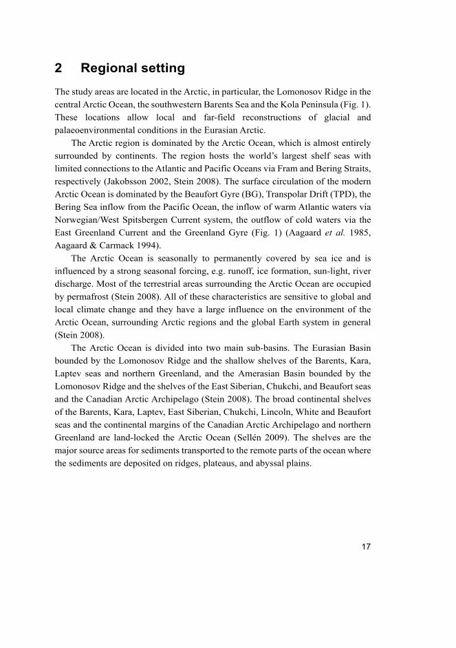
2 Regional setting

The study areas are located in the Arctic, in particular, the Lomonosov Ridge in the

central Arctic Ocean, the southwestern Barents Sea and the Kola Peninsula (Fig. 1).

These locations allow local and far-field reconstructions of glacial and

palaeoenvironmental conditions in the Eurasian Arctic.

The Arctic region is dominated by the Arctic Ocean, which is almost entirely

surrounded by continents. The region hosts the world’s largest shelf seas with

limited connections to the Atlantic and Pacific Oceans via Fram and Bering Straits,

respectively (Jakobsson 2002, Stein 2008). The surface circulation of the modern

Arctic Ocean is dominated by the Beaufort Gyre (BG), Transpolar Drift (TPD), the

Bering Sea inflow from the Pacific Ocean, the inflow of warm Atlantic waters via

Norwegian/West Spitsbergen Current system, the outflow of cold waters via the

East Greenland Current and the Greenland Gyre (Fig. 1) (Aagaard et al. 1985,

Aagaard & Carmack 1994).

The Arctic Ocean is seasonally to permanently covered by sea ice and is

influenced by a strong seasonal forcing, e.g. runoff, ice formation, sun-light, river

discharge. Most of the terrestrial areas surrounding the Arctic Ocean are occupied

by permafrost (Stein 2008). All of these characteristics are sensitive to global and

local climate change and they have a large influence on the environment of the

Arctic Ocean, surrounding Arctic regions and the global Earth system in general

(Stein 2008).

The Arctic Ocean is divided into two main sub-basins. The Eurasian Basin

bounded by the Lomonosov Ridge and the shallow shelves of the Barents, Kara,

Laptev seas and northern Greenland, and the Amerasian Basin bounded by the

Lomonosov Ridge and the shelves of the East Siberian, Chukchi, and Beaufort seas

and the Canadian Arctic Archipelago (Stein 2008). The broad continental shelves

of the Barents, Kara, Laptev, East Siberian, Chukchi, Lincoln, White and Beaufort

seas and the continental margins of the Canadian Arctic Archipelago and northern

Greenland are land-locked the Arctic Ocean (Sellén 2009). The shelves are the

major source areas for sediments transported to the remote parts of the ocean where

the sediments are deposited on ridges, plateaus, and abyssal plains.

18

Fig. 1. Location map of the Arctic region. Study areas are indicated with black frames.

Locations of sites studied (96/12-1pc, BS118, BS231 and BS290) are presented with

white circles. Circulation of the upper layers of the Arctic Ocean is shown with white

arrows and based on the Arctic Monitoring and Assessment Programme image

(AMAP 1998) AMAP. Bathymetry and topography are from the International Bathymetric

Chart of the Arctic Ocean (IBCAO) Version 3.0 (Jakobsson et al. 2012) (Published by

permission of American Geophysical Union).

19

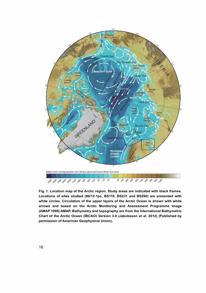
2.1 Lomonosov Ridge

The Arctic Ocean ridges, plateaus, and abyssal plains have a different tectonic

origin and were formed at different times. The Lomonosov Ridge is located in the

central part of the Arctic Ocean and it is a boundary between two Arctic Ocean sub-

basins (Figs 1 and 2).

The Lomonosov Ridge was formed when rifting and seafloor spreading began

to propagate through the Barents-Kara Sea margin and broke off a 1500 km long

continental sliver in the late Paleocene (Wilson 1963, Vogt et al. 1979). Seafloor

spreading moved the Lomonosov Ridge to its present position (Vogt et al. 1979,

Brozena et al. 2003). The oldest sediments were recovered from the Lomonosov

Ridge during the IODP Exp 302, the Arctic Coring Expedition (ACEX). These

sediments are overlaying a regional unconformity, dated around 56 Ma (Backman

& Moran 2009).

Fig. 2. Image reproduced from the International Bathymetric Chart of the Arctic Ocean

(IBCAO) Version 3.0 (Jakobsson et al. 2012) showing a location of core 96/12-1pc.

(Published by permission of American Geophysical Union).

20

The shallowest parts of the Lomonosov Ridge are located off the northern Canada

and Greenland margin, and closer to the North Pole with water depth less than 1000

m. The deepest part of the ridge is also located near the North Pole with a water

depth of 2700 m in the Intra Basin (Sellén 2009). This Intra Basin is characterised

by a sill depth of 1870 m towards the Makarov Basin and the deepest threshold is

2400 m on the Amundsen Basin side (Jokat et al. 1992, Björk et al. 2007, Jakobsson

et al. 2008).

2.2 Barents Sea

The Barents Sea is a shallow epicontinental sea located in the Arctic Ocean. It is

one of the widest continental shelves in the world. The study area is situated in the

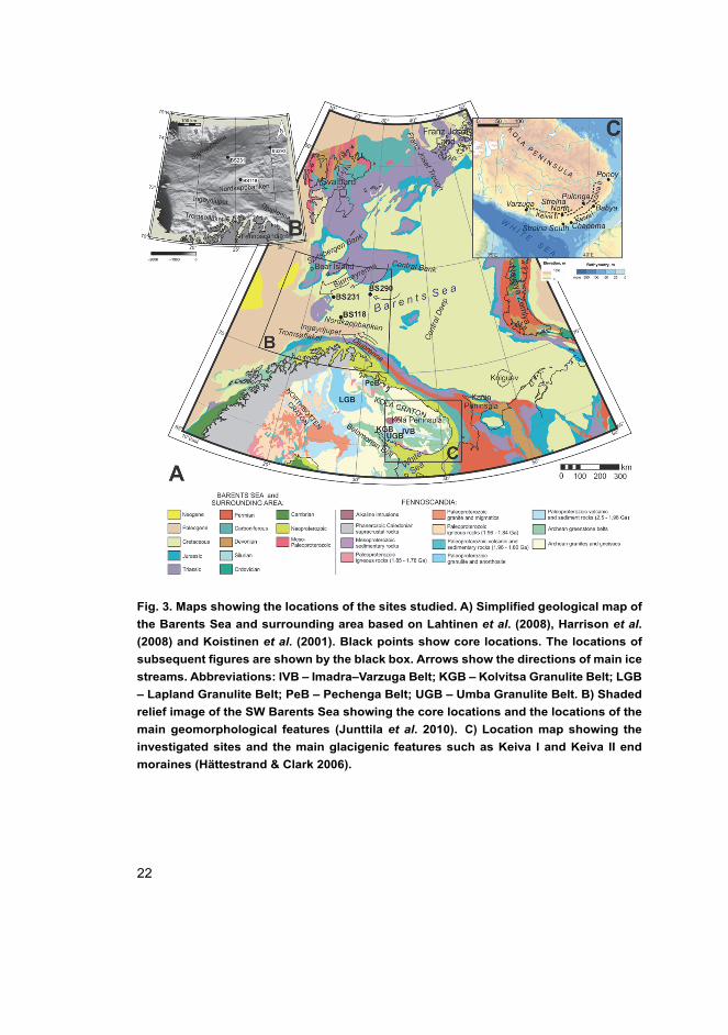
southwestern part of the Barents Sea (Figs 1 and 3A). The major geomorphological

feature of the SW Barents Sea is the Bjørnøyrenna cross–shelf trough (cores BS231

and BS118), which is the main drainage area of the western flank of the Barents-

Kara Ice Sheet (BKIS) (Andreassen et al. 2008), bounded by the shallow

Tromsøflaket and Nordkappbanken banks (Core BS118) to the south (Junttila et al. 2010) (Figs 3A and 3B). The Bjørnøyrenna cross–shelf trough is 750 km long, 150–

200 km wide and the water depth varies between 300 m and 500 m; Tromsøflaket

and Nordkappbanken have water depths of around 200–300 m (Andreassen et al. 2008). The Ingøydjupet (Ingøy Deep) and Djuprenna (Deep Trough) troughs were

the main drainage areas of the northern flank of the Scandinavian Ice Sheet (SIS).

These troughs with water depths of approximately 400 m have southeast–northwest

trends just off the coast of Norway (Andreassen et al. 2008). The main

bathymetrical feature is the more than 400 metre–deep Ingøydjupet trough

bordered by two bank areas to the east and to the west. To the north, the Ingøydjupet

trough terminates in the east–west running Bjørnøyrenna (Vassmyr & Vorren 1990).

Fan–shaped protrusions located at the mouths of the cross–shelf troughs or ‘trough

mouth fans’ (TMFs), characterise the western and northern continental margin of

the Barents Sea – Svalbard area (Vorren et al. 1988, Vorren & Laberg 1997). The

TMFs are sediment depocentres that accumulated in front of ice streams of the

former Fennoscandian – Barents Sea – Svalbard Ice Sheets (Vorren & Laberg 1997,

Vorren et al. 1998, Sejrup et al. 2003, Dahlgren et al. 2005).

Water masses in the SW Barents Sea consist of Atlantic water in the Nordkapp

Current, an extension of the Norwegian Current, lower saline water in the

Norwegian Coastal Current and mixed water masses in the north–east, where the

21

Atlantic, Norwegian Coastal, and Arctic water masses meet (Sakshaug & Skjoldal

1989).

The Barents Sea region is a complex mosaic of basins and platforms that

underwent episodic sedimentation from about 240 Ma to 60 Ma and thereafter

bordered the developing Atlantic Ocean and Arctic Ocean (Doré 1995). According

to Gudlaugsson et al. (1998), the formation of the Barents Sea area consists of three

major phases: the Paleozoic Caledonian Orogeny, the Late Paleozoic – Mesozoic

Uralide Orogeny and major Late Mesozoic – Cenozoic rifting, which led to the

crust breaking up and the current basin configuration. The bedrock in northernmost

Norway and Finland is composed of Archaean and Paleoproterozoic complexes of

the Fennoscandian Shield, Neoproterozoic rocks, and the Caledonides which

extend for several kilometers offshore on the continental shelf (Sigmond 1992,

2002, Siedlecka & Roberts 1996, Koistinen et al. 2001). Onlapping, seaward

dipping sedimentary strata of Late Paleozoic and younger age appears further

offshore (Bugge et al. 1995). More than a thousand metres of Silurian to Pliocene

sedimentary rocks (Vassmyr & Vorren 1990) were eroded during the Quaternary

over large areas of the Barents Sea and distributed outside the shelf edge to the west,

producing the huge Bear Island TMF (Eidvin et al. 1993, 1998, Faleide et al. 1996,

Riis 1996, Vorren & Laberg 1997).

The present geomorphology of the sea floor is shaped by relatively thin

Quaternary sediments overlying bedrock. According to Vorren et al. (1997), the

Bjørnøyrenna Trough Mouth Fan is mostly composed of Cenozoic sediments that

were transported by submarine debris flows during glaciations. Based on work by

Rüther et al. (2011), glaciomarine conditions existed along the western margin of

the Barents Sea at about 17.1–16.6 ka. During this period, a wide sediment wedge

was deposited in Bjørnøyrenna.

The thickness of Quaternary sediments in the Barents Sea is generally less than

100 m. A few metres of sediments mainly deposited during the Late Weichselian

and the Holocene, cover the northwestern regions as well as most of the

topographically high areas of the Barents Sea. These sediments are covered by a

thin drape of Holocene marine sediments (0–10 m) (Vogt & Knies 2009), although,

off the coast, 200–300 m of sediments have been deposited (Sættem et al. 1994,

Elverhøi et al. 1993, Lebesbye 2000).

22

Fig. 3. Maps showing the locations of the sites studied. A) Simplified geological map of

the Barents Sea and surrounding area based on Lahtinen et al. (2008), Harrison et al. (2008) and Koistinen et al. (2001). Black points show core locations. The locations of

subsequent figures are shown by the black box. Arrows show the directions of main ice

streams. Abbreviations: IVB – Imadra–Varzuga Belt; KGB – Kolvitsa Granulite Belt; LGB

– Lapland Granulite Belt; PeB – Pechenga Belt; UGB – Umba Granulite Belt. B) Shaded

relief image of the SW Barents Sea showing the core locations and the locations of the

main geomorphological features (Junttila et al. 2010). C) Location map showing the

investigated sites and the main glacigenic features such as Keiva I and Keiva II end

moraines (Hättestrand & Clark 2006).

23

2.3 Kola Peninsula

The Kola Peninsula is located in the northeastern part of the Fennoscandian Shield

(Figs 3A and 3C). This shield is the largest representative of the Early Precambrian

crystalline basement and supracrustal rocks of the East European Craton.

The northeastern Fennoscandian Shield is divided into three terranes, the

Karelia, Central Kola, and Murmansk Archaean terranes. The Karelia Terrane is a

typical 3.0–2.7 Ga granite-greenstone province. The Central Kola Terrane is a

classic block with amphibolite metamorphism and it consists of various volcanic

and sedimentary rocks with numerous granitoides and gneisses. The Murmansk

Terrane consists of Late Archean granitoid batholits. The Archean nuclei of the

Fennoscandian Shield are overlain by Palaeoproterozoic sedimentary basins and

volcanics (Yakubchuk & Nikishin 2005).

The Palaeoproterozoic sedimentary rocks are widespread in the regions of the

Barents and the White Seas (Mitrofanov et al. 1995). These rocks are cut by

Paleozoic dykes and diatremes. Since Riphean time (1,400–800 Ma), the

northeastern part of the Fennoscandian Shield formed as a stable continental crust

with a constant tendency to uplift. During the Devonian, tectonic-magmatic

activation took place in this region. Volcanic and sedimentary rocks are located

mainly in the area of alkaline plutonic complexes (Mitrofanov et al. 1995). Among

the Mesozoic deposits, kaolins, shungites and phosphates occur in the Kola Region

(Mitrofanov et al. 1995).

Quaternary deposits of the Kola Peninsula contain relics of Paleogene marine

diatoms, indicating that extensive areas of the northern Fennoscandian Shield were

covered by the sea during the Paleogene. The Neogene weathered crust occurs in

the watershed areas, on gentle slopes and on pediment plains. It is assumed that the

area was covered by the SIS many times during the Quaternary. Strelkov et al. (1976) described the distribution of the erratic boulders, the orientation of drumlins,

glacial scars and elongated boulders in till. Till horizons have been encountered at

many sites on the Kola Peninsula and stratigraphically the lowest horizon was

deposited during the Moscowian (Saalian) glaciation (Yevzerov & Koshechkin

1980). Mikhulino (Eemian) interglacial sediments, both continental and marine,

have been found in many localities in the Kola Region. Upper till horizons, upon

Eemian interglacial deposits have been laid down during the Valdai (Weichselian)

glaciation.

24

25

3 Late Pleistocene Arctic climate evolution

Chronological stages of the late Pleistocene (126–11.7 kyr; Cohen et al. 2013)

include two local western European stages of the Eemian intergalacial (Mikulinian

stage in Russia; ca. 126–116 kyr) and the Weichselian cold stage (Valdaian stage in

Russia; 116–11.7 kyr) as well as the Holocene stage (11.7 kyr to present). In the

Arctic, cold glacial conditions dominated during much of the late Pleistocene,

particularly the Weichselian stage. Late Pleistocene environmental conditions were

directly dependent on the rapid and natural climate shifts and transitions from warm

climate to cool climate.

3.1 Late Pleistocene climate shifts

The Quaternary was generally much colder than earlier periods of geological time

and the climate fluctuated from cold to warm many times in different parts of the

world. Many climate fluctuations are recognized during the glacial and interglacial

periods of the Pleistocene, which extends to the latest cold period known as the

Younger Dryas cold spell. Pleistocene climate was marked by repeated glacial

cycles where continental glaciers pushed to the 40th parallel in some places.

Globally, continental ice sheet growth tied up huge volumes of water resulting in

temporary sea level drops of more than 100 meters over the surface of the Earth.

Many different theories have been put forward to explain the onset and termination

of these glacial cycles, for instance, pioneer workers suggested that various

perturbations of the Earth’s orbit around the Sun affected the amount of solar

radiations reaching the Earth which was the primary driver of climate change.

Imbrie et al. (1984) among others showed clear evidence for a close

relationship between orbital cycles and climate changes. The orbital dating of

climate changes are based on variations in planetary motion: eccentricity, obliquity

and precession of the equinoxes based on the Milankovitch hypothesis.

The Milankovitch hypothesis explains long-term climate changes caused

primarily by cyclical changes in the Earth's circumnavigation of the Sun. Three

dominant cycles caused by variations in the Earth's eccentricity, obliquity, and

precession are called as the Milankovitch Cycles. Variations in these three cycles

are reflected in the alterations in the seasonality of solar radiation reaching the

Earth's surface. The first of the three Milankovitch Cycles is named after the shape

of the Earth's orbit around the Sun – eccentricity. The time frame for this cycle is

ca. 98,000 yr. These oscillations, from more elliptic to less elliptic, influence the

26

distance from the Earth to the Sun, changing the amount of radiation received at

the Earth's surface in different seasons. Obliquity is the variation of the tilt of the

Earth's axis from the orbital plane. The obliquity changes on a cycle taking ca.

41,000 yr. Nowadays the Earth's axial tilt is ca. 23.5°, periodic variations of it

explains the Earth's more severe seasons. Precession is the change in orientation of

the Earth's rotational axis. The periodicity of this cycle is ca. 19, 000–23,000 yr.

Precession is caused by two factors – an oscillation of the Earth's axis and a rotation

of the elliptical orbit of the Earth itself. Obliquity affected the tilt of the Earth's axis,

precession affects the direction of the Earth's axis. The change in the axis location

increases the seasonal contrast in one hemisphere while decreasing it in the other

hemisphere.

Changes in the Earth's climate caused by orbital forces were first detected in

marine sediments. Palaeo-ocean temperatures for the Cenozoic were reconstructed

from global deep-sea oxygen (δ18O) and carbon (δ13C) stable isotope

concentrations in benthic foraminifera calcium carbonate shells (Zachos et al. 2001). The isotope ratio 18O/16O or δ18O (‰) record of planktic and benthic

foraminifers represents the cooling and warming of global climate. During

cooler/glacial periods ice sheets expand. This leads to relative 18O enrichment of

the oceanic waters (isotopically positive waters) because large quantities of 16O are

trapped in the ice. During warmer/interglacial periods, the ice sheets retreat. They

melt and liberate large amounts of 16O back into the ocean making the oceanic

waters isotopically negative. The oxygen isotope data from deep-sea core samples

are the basis for creating oxygen stratigraphic scales. Variations in the oxygen

isotope composition are indicated on the curves as specific stages – marine isotope

stages (MIS), first described by Emiliani (1955).

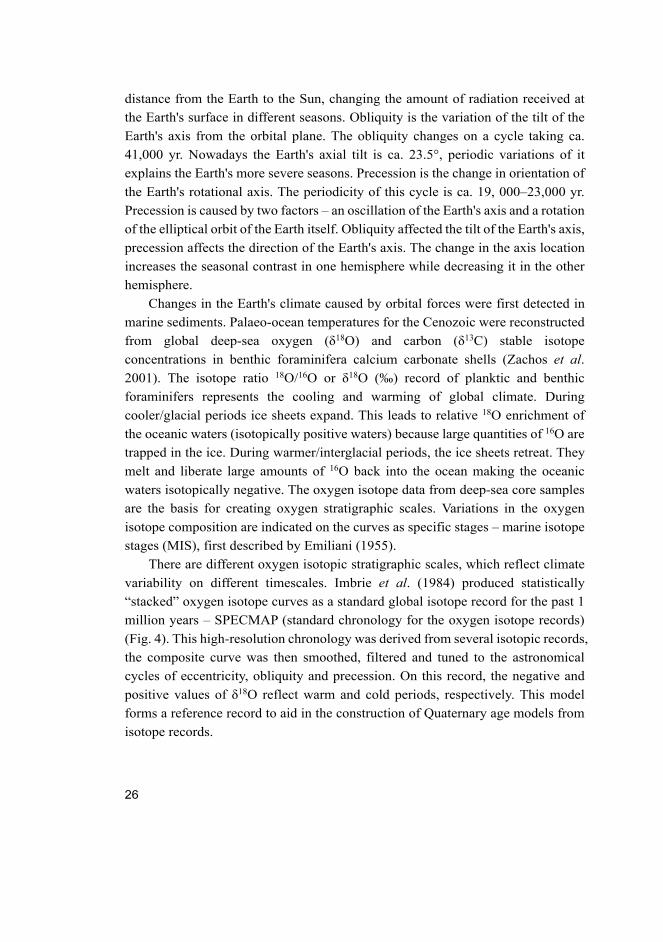
There are different oxygen isotopic stratigraphic scales, which reflect climate

variability on different timescales. Imbrie et al. (1984) produced statistically

“stacked” oxygen isotope curves as a standard global isotope record for the past 1

million years – SPECMAP (standard chronology for the oxygen isotope records)

(Fig. 4). This high-resolution chronology was derived from several isotopic records,

the composite curve was then smoothed, filtered and tuned to the astronomical

cycles of eccentricity, obliquity and precession. On this record, the negative and

positive values of δ18O reflect warm and cold periods, respectively. This model

forms a reference record to aid in the construction of Quaternary age models from

isotope records.

27

Fig. 4. Global deep-sea oxygen (δ18O) observations normalized and plotted on

SPECMAP time scale modified after Imbrie et al. (1984). Late Pleistocene age is

highlighted by grey color.

28

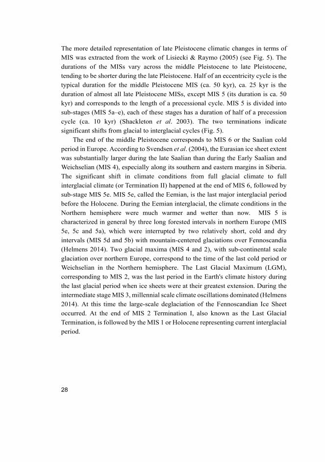
The more detailed representation of late Pleistocene climatic changes in terms of

MIS was extracted from the work of Lisiecki & Raymo (2005) (see Fig. 5). The

durations of the MISs vary across the middle Pleistocene to late Pleistocene,

tending to be shorter during the late Pleistocene. Half of an eccentricity cycle is the

typical duration for the middle Pleistocene MIS (ca. 50 kyr), ca. 25 kyr is the

duration of almost all late Pleistocene MISs, except MIS 5 (its duration is ca. 50

kyr) and corresponds to the length of a precessional cycle. MIS 5 is divided into

sub-stages (MIS 5a–e), each of these stages has a duration of half of a precession

cycle (ca. 10 kyr) (Shackleton et al. 2003). The two terminations indicate

significant shifts from glacial to interglacial cycles (Fig. 5).

The end of the middle Pleistocene corresponds to MIS 6 or the Saalian cold

period in Europe. According to Svendsen et al. (2004), the Eurasian ice sheet extent

was substantially larger during the late Saalian than during the Early Saalian and

Weichselian (MIS 4), especially along its southern and eastern margins in Siberia.

The significant shift in climate conditions from full glacial climate to full

interglacial climate (or Termination II) happened at the end of MIS 6, followed by

sub-stage MIS 5e. MIS 5e, called the Eemian, is the last major interglacial period

before the Holocene. During the Eemian interglacial, the climate conditions in the

Northern hemisphere were much warmer and wetter than now. MIS 5 is

characterized in general by three long forested intervals in northern Europe (MIS

5e, 5c and 5a), which were interrupted by two relatively short, cold and dry

intervals (MIS 5d and 5b) with mountain-centered glaciations over Fennoscandia

(Helmens 2014). Two glacial maxima (MIS 4 and 2), with sub-continental scale

glaciation over northern Europe, correspond to the time of the last cold period or

Weichselian in the Northern hemisphere. The Last Glacial Maximum (LGM),

corresponding to MIS 2, was the last period in the Earth's climate history during

the last glacial period when ice sheets were at their greatest extension. During the

intermediate stage MIS 3, millennial scale climate oscillations dominated (Helmens

2014). At this time the large-scale deglaciation of the Fennoscandian Ice Sheet

occurred. At the end of MIS 2 Termination I, also known as the Last Glacial

Termination, is followed by the MIS 1 or Holocene representing current interglacial

period.

29

Fig. 5. Global deep-sea oxygen (δ18O) record showing climatic stages of the last 200 ka

and middle and late Pleistocene marine isotope stages 1–6 modified after Lisiecki &

Raymo (2005).

3.2 Late Pleistocene Eurasian glaciations

During the Quaternary, vast areas of Eurasia, from mid to high latitudes, were

covered repeatedly by thick and extensive ice sheets (e.g., Svendsen et al. 1999,

2004, Ehlers & Gibbard 2003, 2007, Astakhov 2004, Hughes et al. 2016). Major

glaciations affected the Eurasian Arctic during the last 160 ka years at least four

times (Svendsen et al. 2004). Glacial conditions existed in the Eurasian north

during the late Saalian (before 130 ka) and at least during three intervals in the

Weichselian (at ca. 90–80 ka, 60–50 ka, and 20–15 ka) (Fig. 6) (Svendsen et al. 2004).

30

The interconnected complex of ice sheets in Eurasia are named the Eurasian

ice sheets (EurIS) and described in detail by Hughes et al. (2016) (Fig. 7). The

Scandinavian Ice Sheet (SIS) was the largest component of the EurIS during the

LGM. The smallest component was the British–Irish Ice Sheet (BIIS) which was

connected to the SIS across the North Sea during the late Weichselian. Svalbard,

Barents and Kara ice sheets (SBKIS or BKIS) were located to the north of

Scandinavia (Hughes et al. 2016).

During the late Saalian (160–130 ka), prior to late Pleistocene, a huge ice sheet

complex formed over northern Eurasia (Fig. 6A). A large ice shelf was attached to

the BKIS and possibly extended to the central Arctic Ocean (Svendsen et al. 2004)

(Fig. 6A). However, recent geophysical mapping of glacial features on the seabed,

suggest that the Saalian ice shelf in the Arctic may also have been fed by glacial

ice on the East Siberian continental margin and North America (Jakobsson et al. 2016). The maximum extent of the BKIS during the Early Weichselian (ca. 90 ka)

is shown in Fig. 6B. The major ice dome was located on the continental shelf in the

northern Kara Sea and only a restricted ice sheets existed over Norway, Sweden

and Finnish Lapland (Svendsen et al. 2004). This glaciation was followed by a

major deglacial period during MIS 5a (ca. 85–75 ka). During the middle

Weichselian, a re-growth of the BKIS took place, leading to another ice advance

onto the northern margin of the Eurasian mainland at around 60 ka (Svendsen et al. 2004). The southern margin of the SIS reached Denmark and the eastern flank

covered the whole of Finland, with an ice lobe reaching the White Sea Basin during

this glaciation (Fig. 6C). Major middle Weichselian deglaciation (ca. 60–50 ka)

followed this glaciation. During the late Weichselian glacial maximum or the Last

Glacial Maximum (LGM) (ca. 20–15 ka), the southern and eastern flanks of the

BKIS terminated on the seafloor in the south-eastern Barents Sea and on the

western Kara Sea shelf, far inside its Early Weichselian maximum extent (Svendsen

et al. 2004) (Figs 6D and 7).

31

Fig. 6. Reconstructions of the Eurasian ice sheet extent during the period 140 ka–20 ka

years from late Saalian to Last Glacial Maximum compiled after Svendsen et al. (2004).

A) Reconstructed ice sheet limit in Eurasia during the late Saalian (ca. 160–140 ka). B)

Early Weichselian glacial maximum (90–80 ka). C) Middle Weichselian glacial maximum

(at around 60 ka). D) Late Weichselian glacial maximum (LGM).

According to Hughes et al. (2016), the EurIS started to disintegrate after the LGM

(Fig. 7), and separate ice sheets (i.e. the SBKIS), the SIS and the BIIS formed

during the course of the late Weichselian to the early Holocene. The SBKIS reached

the shelf break twice in the SW of the Barents Sea; first during the LGM at around

22 000 cal. yr B. P. and then at ca. 20 000 cal. yr B. P. (Vorren & Laberg 1996).

Deglaciation of the SBKIS started between ca. 18 700 cal. yr B. P. and 14 000 cal.

yr B. P. (Hald et al. 1989; Vassmyr & Vorren 1990; Vorren & Laberg 1996;

Murdmaa et al. 2006; Junttila et al. 2010). The ice sheets transported debris from

the surrounding areas such as Svalbard, Franz Josef Land and mainly from the

continental territories covered by the SIS, SW of the Barents Sea (Andreassen et al. 2008; Junttila et al. 2010). Active melting of the ice sheets thus led to deposition

of glaciomarine sediments in the SW Barents Sea.

32

Fig. 7. Maximum extent of the ice sheet during the LGM (white lines) at the northern

Eurasia modified after Hughes et al. 2016. Approximate boundaries between three

Eurasian ice sheets – SBKIS, SIS and BIIS – are marked by dashed white lines.

33

4 Coring sites, lithology and age models

The present study combines multi-proxy data obtained from one coring site on the

Lomonosov Ridge, three gravity cores recovered from the SW Barents Sea and

eight sedimentary sections located mainly south and southeast of the Kola

Peninsula adjacent to the White Sea.

4.1 Lomonosov Ridge

A 722-cm-long piston core – 96/12-1pc – was retrieved during the Arctic Ocean-

96 expedition from the crest of the Lomonosov Ridge at 87°05.9’N, 144°46.4’E, at

a water depth of 1003 m, with no evidence of any internal sediment erosion

(Jakobsson et al. 2000) (Publication I).

The core is situated beneath the merging area of sea-ice transported by the

Transpolar Drift (TPD) and the Beaufort Gyre (BG) (Fig. 1). Its location means that

glacial sediments could be derived from any of the glaciated Arctic margins, which

makes provenance analyses particularly important. Core 96/12-1pc recovered late

and middle Pleistocene sediments. This study focused on the interval 42–260 cm

below sea floor (cm bsf), which corresponds to MIS 3–6 in terms of marine isotope

stages. According to the age model of Jakobsson et al. (2000), MIS 3 corresponds

to the depth 42–123 cm bsf; MIS 4 – 123–163 cm bsf; MIS 5 – 163–230 cm bsf;

and the age of sediments at the depth between 230 and 260 cm bsf is estimated as

MIS 6 (Fig. 8).

The core 96/12-1pc sediments (Fig. 8) is mostly composed of horizontally

bedded silty clay and clay (Jakobsson et al. 2000). Between 3 and 115 cm bsf, the

sediments are light brown to light yellowish-brown, mottled clayey silt with faint

horizontal color banding. A homogeneous dark gray silty clay unit occurs around

115–163 cm bsf. There is a significant component of sand–sized quartz and lithic

fragments within these two units (Fig. 8). The lowermost unit has a sharp contact

with an underlying olive to light brown clay between 163–186 cm bsf. The olive to

light brown clay grades into a coarse/grained, light gray/brown sandy clay that

occurs from 186 to 191 cm bsf. There is a sharp contact between this sandy clay

and underlying, thin (1 cm) olive/gray clay, which in turn has a sharp contact with

another 1-cm-thick unit of light brown clay. Between 193 and 722 cm bsf, the

sediment consists of dark brown to medium brown oxidized and bioturbated clay

units alternating with light brown clay. Dark brown clay units below 193 cm bsf

occur in a cyclic fashion. They are 2–14 cm thick and lithologically similar to the

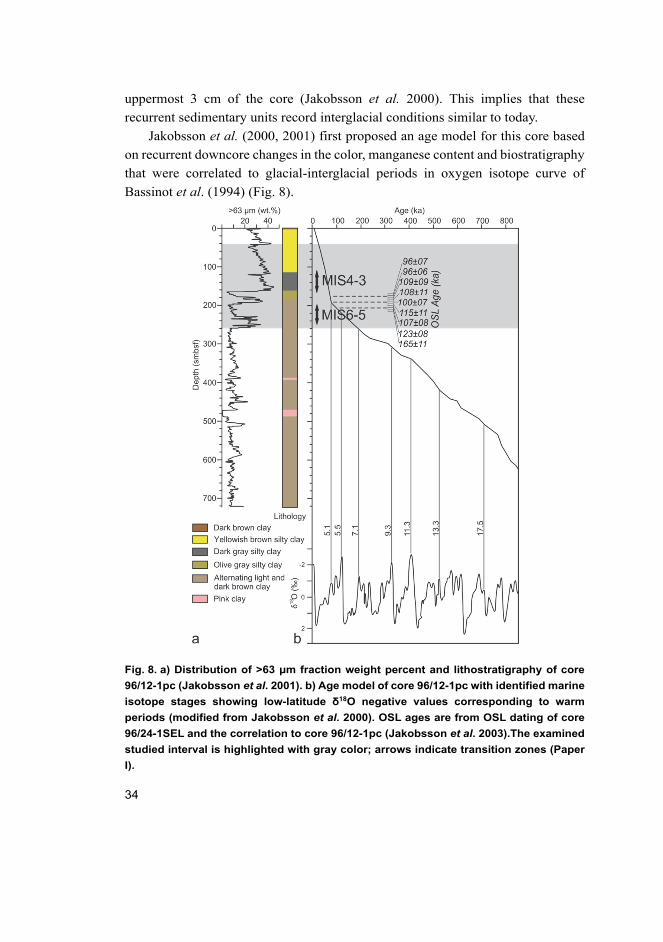
34

uppermost 3 cm of the core (Jakobsson et al. 2000). This implies that these

recurrent sedimentary units record interglacial conditions similar to today.

Jakobsson et al. (2000, 2001) first proposed an age model for this core based

on recurrent downcore changes in the color, manganese content and biostratigraphy

that were correlated to glacial-interglacial periods in oxygen isotope curve of

Bassinot et al. (1994) (Fig. 8).

Fig. 8. a) Distribution of >63 μm fraction weight percent and lithostratigraphy of core

96/12-1pc (Jakobsson et al. 2001). b) Age model of core 96/12-1pc with identified marine

isotope stages showing low-latitude δ18O negative values corresponding to warm

periods (modified from Jakobsson et al. 2000). OSL ages are from OSL dating of core

96/24-1SEL and the correlation to core 96/12-1pc (Jakobsson et al. 2003).The examined

studied interval is highlighted with gray color; arrows indicate transition zones (Paper

I).

35

Later, Jakobsson et al. (2003) also used optically stimulated luminescence

(OSL) for age determination, which supported the established age model. The

obtained age model was compared with glacial intervals recognised along the

Eurasian Arctic margin. The age model yields a sedimentation rate of 2.8 cm/kyr

from MIS 1 through MIS 4 and 0.5 cm/kyr for the time pre-dating prior to MIS 5

to the core bottom. The cause of the sharp change in sedimentation rate at about the

MIS 5–4 transition is due to large amounts of ice-rafted material (Jakobsson et al. 2000) (Fig. 8).

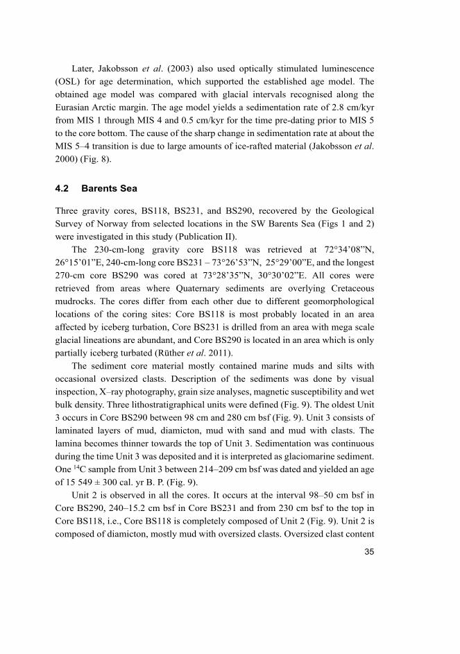
4.2 Barents Sea

Three gravity cores, BS118, BS231, and BS290, recovered by the Geological

Survey of Norway from selected locations in the SW Barents Sea (Figs 1 and 2)

were investigated in this study (Publication II).

The 230-cm-long gravity core BS118 was retrieved at 72°34’08”N,

26°15’01”E, 240-cm-long core BS231 – 73°26’53”N, 25°29’00”E, and the longest

270-cm core BS290 was cored at 73°28’35”N, 30°30’02”E. All cores were

retrieved from areas where Quaternary sediments are overlying Cretaceous

mudrocks. The cores differ from each other due to different geomorphological

locations of the coring sites: Core BS118 is most probably located in an area

affected by iceberg turbation, Core BS231 is drilled from an area with mega scale

glacial lineations are abundant, and Core BS290 is located in an area which is only

partially iceberg turbated (Rüther et al. 2011).

The sediment core material mostly contained marine muds and silts with

occasional oversized clasts. Description of the sediments was done by visual

inspection, X–ray photography, grain size analyses, magnetic susceptibility and wet

bulk density. Three lithostratigraphical units were defined (Fig. 9). The oldest Unit

3 occurs in Core BS290 between 98 cm and 280 cm bsf (Fig. 9). Unit 3 consists of

laminated layers of mud, diamicton, mud with sand and mud with clasts. The

lamina becomes thinner towards the top of Unit 3. Sedimentation was continuous

during the time Unit 3 was deposited and it is interpreted as glaciomarine sediment.

One 14C sample from Unit 3 between 214–209 cm bsf was dated and yielded an age

of 15 549 ± 300 cal. yr B. P. (Fig. 9).

Unit 2 is observed in all the cores. It occurs at the interval 98–50 cm bsf in

Core BS290, 240–15.2 cm bsf in Core BS231 and from 230 cm bsf to the top in

Core BS118, i.e., Core BS118 is completely composed of Unit 2 (Fig. 9). Unit 2 is

composed of diamicton, mostly mud with oversized clasts. Oversized clast content

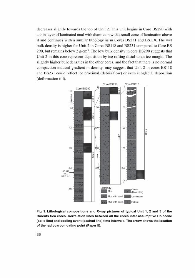
36

decreases slightly towards the top of Unit 2. This unit begins in Core BS290 with

a thin layer of laminated mud with diamicton with a small zone of lamination above

it and continues with a similar lithology as in Cores BS231 and BS118. The wet

bulk density is higher for Unit 2 in Cores BS118 and BS231 compared to Core BS

290, but remains below 2 g/cm3. The low bulk density in core BS290 suggests that

Unit 2 in this core represent deposition by ice rafting distal to an ice margin. The

slightly higher bulk densities in the other cores, and the fact that there is no normal

compaction induced gradient in density, may suggest that Unit 2 in cores BS118

and BS231 could reflect ice proximal (debris flow) or even subglacial deposition

(deformation till).

Fig. 9. Lithological compositions and X–ray pictures of typical Unit 1, 2 and 3 of the

Barents Sea cores. Correlation lines between all the cores infer assumptive Holocene

(solid line) and cooling event (dashed line) time intervals. The arrow shows the location

of the radiocarbon dating point (Paper II).

37

The uppermost Unit 1 occurs in Core BS290 between 50 cm bsf and 10 cm bsf

and in Core BS231 from 15.2 cm bsf to the top of the core and is composed of mud

(Fig. 9).

4.3 Kola Peninsula

Twenty sedimentary sections were logged and measured along riverbank exposures

and gravel pits on the Kola Peninsula, from which eight representative sections

were selected for this research (Table 1, Publication III).

Table 1. Sedimentary sections locations.

Latitude Longitude Exposure

66°25’31.4”N 36°32’04.7”E Varzuga North - Section 1

66°24’46.64”N 36°36’32.6”E Varzuga East - Section 1

66º23’45.5”N 36º39’01.0”E Varzuga South - Section 1

66º23’47.29”N 36º38’56.26”E Varzuga South - Section 2

66º23’47.6”N 36º38’54.4”E Varzuga South - Section 3

66º20’48.4”N 38º37’31.3”E Strelna North

66º29’07.18”N 40º10’22.45”E Babya

66º23’45.5”N 36º39’01.0”E Varzuga South Section 1

67º05’38.81”N 41º05’27.51”E Ponoy

66º33’01.9”N 39º41’30.4”E Pulonga

The studied sections describing the late Pleistocene stratigraphy are located close

to or in the area where the Eemian marine sediments were previously described by

Grave et al. (1969) and Ikonen & Ekman (2001). A clear identification of the

Eemian marker horizon (ca. MIS 5e) was done at two sites, at Varzuga and

Chapoma (Fig. 3). The remaining sediment sections at different sites occur above

the Eemian marker horizon.

The most complete sediment succession showing the history of the last glacial

cycle on the Kola Peninsula is located south of Varzuga village where three sections

were logged (Varzuga South Sections 1–3 in Fig. 10). There are mainly silt, sand

and diamicton units above the marine Eemian mud (Fig. 10).

In the rest of the studied sections (i.e. Varzuga East, Varzuga West, Strelna

North, Babya and Ponoy exposures) and observed sites (Pulonga River and Strelna

South) are located in landforms deposited during the last deglaciation (for site

locations see Fig. 3). Sediments at these sites (Fig. 11) and associated deglacial

landforms, shed light on dynamics of the last deglaciation in the Keiva end moraine

38

zone, which is the major glacial landform complex on the Kola Peninsula.

Stratigraphy and geochronology of the sediments studied on the Kola Peninsula are

presented and discussed in Publication III.

Fig. 10. Stratigraphical logs from Varzuga South, Varzuga North and Varzuga East

exposures (Paper III).

39

Fig. 11. Stratigraphical logs from Strelna North, Babya and Ponoy exposures. See Fig.

10 for the legend (Paper III).

40

41

5 Methods

5.1 Sampling procedure

The sampling procedure for mineralogical analyses was almost the same for core

96/12-1pc (Publication I) and Barents Sea cores BS118, BS231 and BS290

(Publication II). Sediments from core 96/12-1pc were sampled at a spacing ca. 5–

10-cm from the interval 42.5–250.8 cm bsf, which corresponds to ca. 2–4 ka years

according to the sedimentation rate in the age model of Jakobsson et al. (2000). The

Barents Sea core sections were sampled at 10-cm intervals. A total of 24 samples

were obtained from Core BS118 from 1 to 221 cm bsf; 13 samples were taken from

Core BS231 from 1 to 121 cm bsf; the longest Core BS290 was sampled from 12

to 280 cm bsf with a total of 28 samples. Sand-rich sediments collected from the

Kola Peninsula were dated using OSL dating. 12 OSL samples were collected from

8 sections with sand-rich sediments. All methods are described in details below.

5.2 Mineralogical data analysis

5.2.1 Clay mineral analysis

X–ray diffraction (XRD) was performed on oriented clay samples at the Center of

Microscopy and Nanotechnology, University of Oulu, Finland, using the method

described by Hardy & Tucker (1988) and Moore & Reynolds (1997) (Publication

II).

A total of 75 samples from Cores BS118 (23 samples), BS231 (24 samples),

and BS290 (28 samples) were analysed. The sample preparation procedure

included the following steps for each sample. Three grams of sediment was

weighed, distilled water was added and the sample was stirred with a glass rod until

suspension. The sample was then transferred to a centrifuge tube and centrifuged

for 1 minute (at 1000 rpm according to Stoke's law) to settle all the particle sizes

larger than clay–size to the bottom of the centrifuge tube and leave clay particles

in suspension. The suspension was removed from the centrifuge tube and placed

into another tube. The samples were then concentrated by centrifugation for 15 min

(1000 rounds/minute) to settle the clay to the bottom of the tube, after which the

water was decanted. Then the oriented clay samples were made on glass slides.

Three different preparations were made: air–dried or normal, heated, and ethylene

42

glycol treated. Air dried samples were placed in a drying oven at 60°C for two

hours. The heated samples were first dried in the oven at 60°C for one hour and

later heated to 550°C for an additional two hours. This heating caused the kaolinite

structure to collapse. The ethylene glycol–treated samples were placed into a

special container, which was placed in the oven at 60°C and kept there until the

samples were ready for analysis. The ethylene glycol caused the smectite in the

sample to expand its basal spacing from 10 Å to about 17 Å, which makes it

recognisable in a diffractogram. The air–dried or normal samples were the standard.

Both the normal and heated samples were stored in a desiccator until they were

ready to be analysed (Hardy & Tucker 1988).

Diffractograms were recorded by a Siemens D 5000 XRD Diffractometer with

a fixed divergence slit (FDS), with copper radiation (40 kV, 40 mA) at angles

ranging from 2° to 32° 2θ (0.02° 2θ per second). The four principal clay mineral

groups were recognized by their basal spacings at 7 Å (kaolinite and chlorite), 10

Å (illite), 15–17 Å (smectite), and 14 Å (chlorite). In this paper, chlorite was

identified at 3.54 Å and kaolinite at 3.58 Å (Biscaye 1964), and the peak–area

method was used to calculate the quantities of kaolinite and chlorite from the joint

peak at 7 Å. The ethylene glycol–treated sample was used to distinguish between

the four clay minerals.

MacDiff software version 4.2.5 was used to quantify the clay minerals

(http://www.geologie.uni–frankfurt.de/Staff/Homepages/Petschick/RainerE.html),

which were subsequently used to calculate percentages using weighting factors

(Biscaye 1965). This software analysed the glycollated preparation from the

diffractogram as the peaks are best defined there. The analysed clays were

evaluated by peak fitting, an evaluation method based on Pseudo Voigt functions

in the MacDiff software, which is often used for calculations of experimental

spectral line shapes. Peak fitting makes an evaluation of the smectite peak (15–17

Å) possible without any interference by the chlorite peak (14 Å). Since no internal

standards were used, the accuracy of this procedure is not known, but the semi–

quantitative analyses justify interpretations of fluctuations around ± 2%.

5.2.2 Heavy mineral analysis

The sample preparation procedure included the following steps. Each sample was

first disaggregated using distilled water and a dispersant. Then the sediment was

soaked in a plastic test tube containing 40–60 ml of distilled water and 2 ml of

dispersant solution. One litre of the dispersant solution contained 33 g of sodium

43

hexametaphosphate ((NaPO3)6), 7 g of sodium carbonate (Na2CO3) and distilled

water. Aggregates were removed by soaking a 3-g sediment sample 1–2 hours in a

solution prepared by mixing 40–60 ml of distilled water and 2 ml of dispersant

solution. The samples were centrifuged three times for 1 minute to suspend and

remove the clay fraction. After that, they were wet-sieved using a 0.06 mm sieve

and distilled water to remove the silt fraction, dried and collected for heavy liquid

separation. Each of the > 63 μm fraction samples was poured into a small separating

funnel consisting of heavy liquid – sodium heteropolytungstate (LST Fastfloat) –

with a density of 2.82 g/cm3. The mixture was stirred thoroughly with a glass rod

and left for 3 hours to allow the heavy minerals to separate from the light minerals.

After separation, the heavy fraction was drained quickly and carefully onto a filter

paper and cleansed with distilled water using a Buecher funnel for filtration. The

filter paper with the mineral fraction on it was dried at 60°C and the dry fraction

was collected into a test tube.

Heavy minerals were analysed according to the method of Mange & Maurer

(1992). The heavy mineral grains in the medium sand fraction (0.63 mm–0.2 mm)

from 35 samples from core 96/12-1pc (Publication I) and 65 samples from Barents

Sea cores (Publication II) were analysed with the electron microprobe (JEOL JXA-

8200) at the Center of Microscopy and Nanotechnology, University of Oulu, using

an accelerating voltage of 16 kV, a beam current of 15nA and a beam diameter of

10 μm.

In total 17 analysed oxides and elements expressed in wt.% – F, Na2O, Al2O3,

MgO, SiO2, Cl, K2O, CaO, TiO2, V2O3, Cr2O3, MnO, FeO, NiO, ZnO, Zr2O, P2O5

– are used for mineral determination. Heavy minerals were identified using

MinIdent-Win 4.0 computer software (Smith & Higgins 2003). The composition of

dolomite, zircon, and apatite was confirmed by using energy-dispersive

spectrometry (EDS). The abundance of each identified mineral was calculated as a

relative percentage of the total grains (n=60) counted for each sample. The quantity

of total grains (n) is low due to the sediment composition containing mostly clay

fraction. Heavy minerals include groups of amphiboles (Ca- and Mg-Fe

amphiboles), garnets (Ca-, Fe-, Mn-garnets), pyroxenes (clinopyroxenes and

orthopyroxenes), epidote, Fe oxides, phyllosilicates, phosphates (mostly apatite),

ilmenite, titanite, carbonates, zircon, oxides (anatase, rutile, chromite, ulvospinel,

etc.) and others (kyanite, andalusite, sillimanite, cordierite, staurolite, monazite,

arsenate, tourmaline, olivine, wolframite, etc.). Analytical error bars of calculations

were estimated as a confidence interval for each group of minerals (Folk 1980).

44

The provenance–sensitive heavy mineral ratios RuZi (rutile:zircon index) and

CZi (chrome–spinel:zircon index) were determined following Morton &

Hallsworth (1994, 1999) for Barents Sea cores (Publication II). Rutile–zircon index

was counted as 100 × rutile count/ (total rutile plus zircon), and chrome–spinel–

zircon index was counted as 100 × chrome–spinel count/ (total chrome–spinel plus

zircon).

5.3 Chronological methods

Optically Stimulated Luminescence (OSL) dating (Publications I and III) and

Accelerator Mass Spectrometry (AMS) radiocarbon dating (Publication II) were

used to establish the chronology of the studied sediments.

Jakobsson et al. (2003) used OSL for age determination of the central Arctic

Ocean sediments. This chronological method offers independent age control for

clastic sediments (Murray & Olley 1999, 2002). The build up of a trapped electron

population in natural minerals, for example, quartz, is used as a chronometer.

During transport by ice, wind or water, for instance, the electron population is

initially set to zero by daylight exposure. This electron population increases with

time due to the exposure to naturally occurring radiation from sediments

(Jakobsson et al. 2003). Much of the present interpretation of the timing of the last

glacial cycle in the Eurasian Arctic is based on the OSL dating (Alexanderson et al. 2001, Houmark-Nielsen et al. 2001, Mangerud et al. 2001). Samples for OSL

dating were extracted from core 96/24-1sel adjacent to our core 96/12-1pc. Core

96/24-1sel was raised from the Lomonosov Ridge at 87.183° latitude and 144.606°

longitude (water depth 980 m) during the Arctic Ocean 96 expedition using the

Swedish icebreaker Oden (Jakobsson et al. 2003). The 400 cm long and 10 cm

diameter core was contained in a black, nontransparent plastic core liner. After that,

it was split and sampled for OSL dating in a dark room at the Nordic Laboratory

for Luminescence Dating (Risø, Denmark). For the detailed description of the

methodology see Jakobsson et al. (2003). The final age model of core 96/12-1pc

was derived by correlating changes in sediment Mn concentration with marine

isotope stages in the low-latitude δ18O stack, with negative values corresponding to

warm periods.

Investigated Barents Sea sediments (Paper II) did not contain any organic

materials, except the interval between 209 cm and 214 cm in Core BS290, which

had enough mixed benthic foraminifera for Accelerator Mass Spectrometry (AMS)

radiocarbon dating. The radiocarbon date of one sample was obtained by the

45

Poznań Radiocarbon Laboratory. The content of 14C in a sample of carbon was

measured using the spectrometer Compact Carbon AMS (produced by National

Electrostatics Corporation, USA) described in the paper by Goslar et al. (2004).

The measurement was performed by comparing intensities of ionic beams of 14C, 13C and 12C measured for each sample and for standard samples. The obtained

radiocarbon date was calibrated using Calib 7.1.0 and a MARINE13 calibration

curve (Hughen et al. 2004, Reimer et al. 2004). We used a marine reservoir age of

467 ± 41, representative of the northern Norway seas (Mangerud & Gulliksen 1975,

Reimer & Reimer 2001).

Dating of sand-rich sediments (Publication III) was carried out using OSL

dating. Twelve OSL samples were collected from 8 sections with sand-rich

sediments. The samples were taken by hammering a dark grey PVC tube (diameter

75 mm, length 350 mm, wall thickness 4 mm) into a sand facies, both ends were

closed with plastic lids and the tubes were carefully wrapped with an aluminum

foil and placed into black plastic bags. Age determinations of the OSL samples

were carried out in the Nordic Laboratory for Luminescence Dating, Risø National

Laboratory Denmark under Dr. A. Murray. The laboratory was also responsible for

the quality control of samples dated.

All OSL samples were prepared under the low-level orange light. The light

exposed ends of the samples were retained for water content and dose rate analysis.

The remaining portion was wet sieved to recover grains 180–250 μm in diameter.

This fraction was etched with HCl, H2O2, HF and again with HCl to obtain a quartz-

rich separation. After chemical separation, samples had a detectable IR-stimulated

signal, indicating residual feldspar contamination. As a result, during routine

measurement, all blue light stimulation was preceded by an infrared stimulation at

125°C (Wallinga et al. 2002).

OSL measurements were carried out on Riso TL/OSL readers, each equipped

with a calibrated 90Sr/90Y beta radiation source and a blue (470 ± 20nm) light source

(Bøtter-Jensen et al. 2000). Prepared quartz grains were attached in a monolayer to

ca. 10 mm diameter stainless steel (approximately a few thousand grains), using

silicone oil. A SAR-protocol (Murray & Wintle 2000, 2003) was used to estimate

all equivalent doses, with a 260°C for 10 seconds, and a cut heat of 160°C. Dose

rates were derived from radionuclide concentrations, measured by high-resolution

gamma spectrometry (Murray et al. 1987), using conversion factors from Olley et al. (1996). These were modified by attenuation factors based on the observed

sediment water contents (between 21–28%). Finally, the internal alpha radiation

46

contribution (assumed to be 0.06 ± 0.03 Gy) and the calculated cosmic ray dose

rate (Prescott & Hutton 1994) were added to the dose rates.

5.4 Statistical data analysis

Principle component analysis (PCA) was performed for cores BS118, BS231 and

BS290 to explore the relationships between heavy and clay mineral assemblages

and assumed provenances (Publication II).

This analytical work might also show similarities in heavy and clay mineral

assemblages between different lithostratigraphic units, and thus provide material

for correlation purposes and assist in characterizing the source rocks in each

assumed provenance. PCA is a method commonly used in pollen analysis (e.g.,

Lisitsyna et al. 2012; Svendsen et al. 2014) and microtextural analysis (e.g.,

Immonen et al. 2014), providing a simple representation and fast classification of

complex data. For PCA of heavy and clay minerals in 3 Barents Sea cores the

XLSTAT 2017 was used (https://www.xlstat.com/en/). PCA calculated principal

components by reducing the number of variables to a few uncorrelated variables

that are linear combinations of the initial variables. PCA forms new axes through

the data set such that the Axis 1 is in the direction of greatest variance. The Axis 2

which captures a smaller amount of variance than Axis 1, is perpendicular to the

first Axis 1. Interpretation of the PCA axes is usually done according to the contents

or variables they captured.

5.5 Sedimentological observations

Sedimentological investigation of sediment exposures is one of the methods used

in Paper III. Eight representative sections were selected from the twenty

sedimentary sections, which were logged and measured along the riverbank

exposures and gravel pits in the Kola Peninsula. The field work included the

determination of thickness, bedding plane attitude, nature of basal contact, texture,

structure and the lateral extent of each unit, as well as measurements of

palaeocurrent directions from current induced structures. The unit geometry was

also defined when possible. Observations (facies analysis methods) were used in

order to find out contemporary sedimentary environments into which the sediments

under study were deposited.

The measurements of till clast fabric and the orientation of glaciotectonic

structures related to diamicton units were done in order to clarify ice movement

47

directions. Till clast fabric measurements were performed measuring orientation

and dip direction of a-axes of elongated clasts as outlined in Andrews (1971). In

addition, the dip direction of thrust planes and fold axis from glaciotectonically

deformed sediments beneath diamicton units were measured. The facies code

scheme modified after Miall (1977, 1985, 1996) and Eyles (1983) was used to

illustrate the major textural and structural characteristics of sedimentary units. The

full key for the codes is shown in Fig. 10 legend.

5.6 Pollen data analysis

Organic bearing fine sediments at Varzuga South exposure were analysed for their

pollen content (Paper III). The laboratory treatment followed conventional analysis

methods outlined in Berglund & Ralska-Jasiewiczowa (1990). A total of 32 pollen

samples were counted; the volume of sediment in 163 samples varied between 1 to

2 cm3. The slides with samples were mounted in glycerine. 400x magnification was

used for pollen determination; for some critical determinations, the magnification

was 1000x. Pollen identification follows the keys and illustrations in Moore et al. (1991), Reille (1992) and Faegri & Iversen (1989). The number of terrestrial pollen

counted was more than 1000 pollen per each sample. The calculation of pollen

percentages was based on the total sum of terrestrial pollen taxa. The pollen

diagram was constructed using the TILIA computer software (Grimm 1991). Only

selected taxa were presented in the pollen diagram from Varzuga South section in

paper III and the results are compared to a previously published pollen diagram

from the same area by Armand & Lebedeva (1966).

48

49

6 Results: Summary of publications I–III

This thesis contains three papers with different focuses and methodologies,

connected by an idea to detect climate, environmental and ocean circulation

consequences related to the development of late Pleistocene Eurasian ice sheets.

Publication I focuses on two time intervals during the late Pleistocene, specifically,

transitions from glacial to interglacial during (MIS 6–5) and (MIS 4–3) in the

central Arctic Ocean. Changes in sediment provenances in relation to ice flow

patterns and ice rafting from different regional sectors during the Late Glacial to

Holocene in the SW Barents Sea are discussed in Publication II. The evolution of

late Pleistocene palaeoenvironments and the last deglaciation history of the Kola

Peninsula, Russia, are presented in Publication III.

6.1 Publication I: Provenance analysis of central Arctic Ocean

sediments: Implications for circum-Arctic ice sheet dynamics

and ocean circulation during Late Pleistocene

Publication I focuses on the description of sediment provenances shifts within two

late Pleistocene transitions MIS 6–5 and MIS 4–3 in the central Arctic Ocean. To

evaluate ice transport from the circum-Arctic sources and variability in sediment

drainage and provenance changes mineralogical and geochemical data generated

from core 96/12-1pc on the Lomonosov Ridge, central Arctic Ocean was used.

These data are presented by detailed lithostratigraphical observations, age model

and results of heavy mineral analysis.

The identified heavy minerals were divided into two principal groups of major

silicates and other minerals. The distribution of heavy minerals varies over a wide

range throughout the analysed column. The two transitions – MIS 6–5 and MIS 4–

3 – were examined in more detail than the rest of core. The geochemical

compositions of the identified heavy minerals were also compared with those of

source rocks obtained from literature datasets of prominent circum-Arctic

provenances.

The obtained results show changes in transport pathways and source areas

within the two examined transitions. The main source for material during the MIS

6–5 transition was the Amerasian margin due to the high dolomite content in the

sediments inferring a strong BG and TPD transport for this material. The transition

from MIS 4–3 shows a clear shift in source areas, reflected in a different

mineralogical composition of sediments, supplied from the Eurasian margin during

50

the active decay of the BKIS. This may reflect enhanced sediment input from an

ice-dammed lake outburst and a strong TPD over the central Arctic. These two

studied deglaciations suggest that contributions of different circum-Arctic sediment

sources are related to the interaction between ice sheet decay, sea ice production,

and circulation. They highlight how provenance studies in far-field locations can

be used to identify glacial activity on different margins of the Arctic.

6.2 Publication II: Provenance signatures and changes of the

southwestern sector of the Barents Ice Sheet during the last

deglaciation

Publication II combines data from sedimentological, mineralogical (including clay

and heavy minerals) and numerical analysis of samples selected from three gravity

cores, BS118, BS231, and BS290 in the SW Barents Sea. The sediments studied

are subglacial/glaciomarine to marine in origin.

Physical properties of the sediments, including magnetic susceptibility and wet

bulk density, were measured prior to opening. Radiocarbon dating was done using

AMS method only for one sample due to the lack of organic material. Mineralogical

analyses include clay and heavy mineral analyses carried out for samples from all

studied cores. Numerical analysis presented by principle component analysis was

performed for all identified heavy and clay minerals to explore the relationships

between heavy and clay mineral assemblages and assumed provenances.

The core sequences were divided into three lithostratigraphic units. The lowest,

Unit 3, consists of laminated glaciomarine sediments related to regional

deglaciation. Overlaying Unit 2 is composed of diamicton, dominated by mud and

oversized clasts, and is interpreted to reflect a more ice-proximal sedimentary

environment or possibly subglacial deposition. The genesis of Unit 2 varies

between cores, which indicates an influence of different ice flow sectors in the

depositional area. Its deposition may indicate a glacial re-advance or stand still

during an overall retreat. The uppermost Unit 1 consists of Holocene marine

sediments and currently reworked sedimentary material with a relatively high

carbonate content.

Our results, based on clay minerals and varietal studies of heavy minerals,

indicate that the provenance areas can be reliably related to certain ice flow sectors

and transport mechanisms in the deglaciated Barents Sea.

51

6.3 Publication III: Late Pleistocene palaeoenvironments and the

last deglaciation on the Kola Peninsula, Russia

In Paper III the lithostratigraphical and sedimentological observations obtained

from land sections located in the southern part of the Kola Peninsula are presented

to shed light on palaeoenvironmental development during the late Pleistocene from

the Eemian interglacial to the Holocene.

To clarify the pattern and timing of the last deglaciation and the age of the

Keiva end moraines, the sand sediments were dated with OSL method. Other

methods used in this work include onsite sedimentological investigations of

sediment exposures. Thickness, bedding plane attitude, nature of basal contact,

texture, and structure and the lateral extent of each unit were determined in the field

and paleocurrent directions were measured from current induced structures. The

unit geometry was also defined when possible. Observations (facies analysis

methods) were used in order to find out contemporary sedimentary environments

into which the sediments under study were deposited. Additionally, the organic

bearing fine sediments at Varzuga South exposure were analysed for their pollen

content.

The results indicate that the Eemian marine environment in the onshore coastal

areas gradually changed into a glaciolacustrine environment. The first ice advance

into the western part of the study area took place already during the Early

Weichselian. After deglaciation of the Early Weichselian ice, glaciolacustrine

conditions were re-established. The second ice advance into the area took place

most probably during the late Weichselian, although the sedimentary record does

not exclude the possibility that ice also advanced onto Kola during the middle

Weichselian. The southern and central coastal areas of the Kola Peninsula were

deglaciated between 16 ka to 12 ka. The most prominent end moraine ridges, the

Keiva II and Keiva I end moraines were deposited in an interlobate zone between

the ice mass in the interior of Kola and the White Sea ice lobe during the Younger

Dryas.

52

53

7 Discussion

In this chapter, deglaciation of late Pleistocene Eurasian ice sheets in three

investigated areas – the central Arctic Ocean, SW Barents Sea and Kola Peninsula

– is broadly reviewed, in an attempt to achieve the main aims of the research, which

is the reconstruction of interactions between components of the EurIS and their

development during the past 160 ka years. The interpretations and further

discussion of the obtained results are based on the explanation of provenance

changes induced by EuIS deglaciation in the central Arctic Ocean and SW Barents

Sea and description of sedimentation conditions during the late Pleistocene

deglaciation on the southern part of the Kola Peninsula.

7.1 Shifts in the central Arctic provenances during the Late

Pleistocene

Several circum-Arctic provenance changes throughout the analysed core were

defined based on changes in heavy mineral assemblages. The pathways for mineral

supply in the central Arctic Ocean are mainly sea ice and icebergs from ice sheet

decay. The transported material from continental margins to the central part of the

Arctic Ocean is carried by ocean currents. According to Bischof & Darby (1997),

sea ice mainly follows the iceberg trajectories. The two main wind-driven surface

circulation systems in the Arctic Ocean are the clockwise BG in the western Arctic

and the TPD that carries water and ice from the Siberian margin to the Norwegian-

Greenland Sea through the central Arctic (Schoster et al. 2000, Adler et al. 2009).

These two ocean circulation systems are the main agents that transport sea ice and

icebergs with entrained sediment material from the Eurasian marginal seas – such

as the Laptev Sea and Kara Sea – and the Amerasian side.

The provenances that supplied the material to the central Arctic Ocean during

the two intensively studied transitions (MIS 6–5 and MIS 4–3) are represented by

four areas or end-members whose relative contributions were estimated according

to the presence of various heavy mineral assemblages. The Amerasian source area

including the MacKenzie River basin with Banks and Victoria islands is

represented mostly during the MIS 6–5 transition. The input from Eurasian sources,

i.e. the Anabar massif, the Putorana Plateau, and the Verkhoyansk Fold Belt, varies

throughout the examined time interval and reflects changes in sediment supply

areas and sediment transport pathways.

54

In comparison with previously studied end-member contributions to the central

Arctic Ocean (northern Mendeleev Ridge) based on Nd and Pb isotope fingerprints

of detrital fractions (Fagel et al. 2014), the analysed sediments from the

Lomonosov Ridge came from several different sources. Fagel et al. (2014)

subdivided the central Arctic Ocean sediment sources into 3 end-members,

including the North American margin represented by the MacKenzie River

sediment source, the crustal Eurasian margin sources with the Lena River signature,

and the volcanic province near the Okhotsk-Chukotka Arc. The Lomonosov

Ridge's detrital sediments are composed of material from the same North American

and Eurasian sources. In addition to the Eurasian sources, the input of material from

the Anabar Shield, the Putorana Plateau and the Verkhoyansk Fold Belt were

considered, but material of volcanic origin was not discovered in the Lomonosov

Ridge sediments. Estimated relative contributions of the four end-members

confirms that the sediment provenances and ice sheet behaviors in the central Arctic

Ocean during the late Pleistocene can significantly differ between

interglacial/deglacial transitions. From these transitions, MIS 6–5 records

significant sediment input from the American margin, indicated by the high input

of detrital carbonate material and dolomite, as well as rather constant supplies from

the Eastern Eurasian margin. The provenance of the carbonates was probably the

southwestern Canadian Arctic Archipelago, in particular, Victoria Island (Bischof

et al. 1996).

In contrast, glacial conditions during MIS 4 record maximum supplies only

from the Eurasian continent. It is also clearly seen during the MIS 4– 3 transition,

that significant amounts of sediment were derived from the Anabar Shield and the

Putorana Plateau. The obtained results support the idea that the Eurasian margin

contributed most of the sediment to core 96/12-1pc, being consistent with results

by Spielhagen et al. (2004), Krylov et al. (2008) and Martinez et al. (2009), but

that at times, a North American source dominated. During interglacial and late

deglacial Ameriasian sources became a significant component of terrigenous input,

possibly through the MacKenzie route described by Not & Hillaire-Marcel (2012).

7.2 SW Barents Sea provenance changes during the BKIS and SIS

deglaciation

The existence and deglacial history of the BKIS and SIS during the late Pleistocene

are described in the context of three time intervals, namely the deglaciation phase,

the ice re-advance phase, and the Holocene.

55

The deglaciation phase corresponds to the time of Unit 3 deposition. A similar

unit was established by Vorren et al. (1984), Thomsen & Vorren (1987), Hald &

Vorren (1987), Murdmaa et al. (2006), Vassmyr &Vorren (1990) and Winsborrow

et al. (2010). The overlying sediments of Unit 2 represent the ice-re-advance phase

and could correspond to the unit 2 distinguished in the Barents Sea sediments by

Elverhøi et al. (1993), Murdmaa et al. (2006) and Winsborrow et al. (2010). Unit

1 correlates with Holocene units established by Vassmyr & Vorren (1990), Elverhøi

et al. (1993), Murdmaa et al. (2006) and Winsborrow et al. (2010).

Sediments of Unit 3 were deposited during the deglaciation phase, probably

between 16 and 13 ka cal. yr B. P. and characterized by deposition of glaciomarine

sediments with sparse fauna. The exact timing of the deglaciation is unknown; a

radiocarbon date in the interval between 209 cm and 214 cm in Core BS290 (Unit

3) gives an age of 15 549 ± 300 cal. yr B. P. The core location was ice free prior to

and after this date based on the lithological composition of the sediments. The

BKIS and SIS were retreating before this date, making at least one core location

(core BS290) in the Barents Sea free of ice sheet cover. This change in

palaeogeographic conditions is reflected in the sediment composition. The high

IRD content within all the time intervals indicates that icebergs supplied material

throughout deglaciation and were in a proximal location to the investigated area.

These changes in clay and heavy mineral compositions also indicate changes in the

source areas. Fennoscandian sources, Svalbard, Franz Josef Land and outcrops of

the Barents Sea Shelf were the most important source areas prior to ca.15 500 cal.

yr B. P. based on heavy and clay minerals. After ca. 15 500 cal. yr B. P., Svalbard

and Franz Josef Land were minor sources of sediment, with almost all the material

being derived from Fennoscandian sources fed into the SW Barents Sea by icebergs

and ocean currents. An exception is kaolinite, which could have been transported

from northern sources (Ślubowska–Woldengen et al. 2008), i.e., Svalbard.

The peak values in smectite content might indicate increased inflow of Atlantic

water masses due to the opening of the Barents Sea, and as a result, transport of

fine fraction sediments from the Vøring Plateau (Vogt & Knies 2009, Junttila et al. 2010).

Unit 2 was deposited, perhaps, during still stands or ice advance periods and

intensive melting of ice after this, which is suggested by the high IRD content.

These sediments were deposited by the SIS, most probably during the Younger Dryas

ice advance. This assertion is based on the presence of a high amount of IRD and would

have been followed by ice stream retreat from the shelf area to the inner fjord area

(Vassmyr & Vorren 1990). Core BS290 is located in the proximity of grounding

56

zone wedges according to maps by Winsborrow et al. (2010). These grounding

zone wedges were formed by still stands of the retreating ice sheet and intensive

processes of melting. The increased content of IRD offshore supports the idea of

Weichselian ice advances from which IRD sediments were deposited mostly by

icebergs (Vassmyr & Vorren 1990). According to reconstructions of the SIS by

Hughes et al. (2016), re-growth during the cooling event after our dating ca. 15 500

cal. yr may have been from Norwegian fjords, Porsangerfjorden, Lakselvfjorden,

and Tanafjorden, in particular. Icebergs released from these fjords and valleys

transported IRD material from Fennoscandian sources to the SW Barents Sea. The

SIS produced the crystalline clasts that were transported and deposited in the study

area, which is also confirmed by the heavy mineral content. Most of it

corresponding to the heavy minerals of Fennoscandian origin, evidenced by the

high content of Fe oxides, and also prominent Svalbard and Franz Josef Land

origin, evidenced by the increasing kaolinite content due to glacial erosion. Illite

content within this time interval is constant, which might indicate meltwater

discharge from the continent, and smectite content is related to ocean current

transportation (Junttila et al. 2010).

In sediments of Unit 1, possibly deposited during the Holocene to present,

almost no IRD was found in Cores BS290 and BS231. Sporadic occurrence of IRD

and heavy minerals in this interval is mostly due to the reworking by bottom

currents. Clay sedimentation was under the influence of surface ocean currents

controlled by winds and related sea ice transportation. The sediments within Unit

1 show that clay mineral contents are stable, which can be explained by ocean

current transportation of illite and smectite. The prevalence of illite within this time

interval is due to meltwater discharge from the continent (Junttila et al. 2010). The

Barents Sea was free of an ice sheet during this time. The inflow of warm Atlantic

water is reflected by the deposition of a biogenic carbonate fraction found within

the muds. The same process was described by Vassmyr & Vorren (1990), and

episodic deposition of foraminifera in the Barents Sea during the Holocene was

found by Rüther et al. (2012).

7.3 Late Pleistocene palaeoenvironments and sedimentation

processes in the southern part of the Kola Peninsula

To unravel the late Pleistocene history of the southern Kola Peninsula and the White

Sea Basin, the Varzuga South exposure was studied as a key section. The Eemian

marine sediments at the base of the Varzuga South exposures are correlative to

57

marine mollusc bearing sediments at Chapoma and other Eemian marine deposits

in NW Russia (Ikonen & Ekman 2001). At Chapoma, the Eemian marine sediments

rest on a till unit, which was most likely deposited during the Saalian glaciation.

The Eemian sediments at Varzuga South are thought to have been deposited in a

deeper water (depth 40–50 m) compared to those sediments at Chapoma which,

according to diatom taxa, were deposited in a littoral zone influenced by river water

(Cheremisinova 1962).

In the previous investigation of the Varzuga River exposures at the Koitugov

Rapid area (Apukhtin 1978), the change from the Eemian marine muds into

laminated silt and clay were not possible to detect since the exposures were severely

glacitectonized. According to Apukhtin (1978), clay- or sand-rich till overlies the

Eemian marine mud at the Koitugov Rapid exposures. However, a continuous

sediment sequence at Varzuga South with an occurrence of dropstones in silt and

clay rhythmites indicates that the warm Eemian marine environment gradually

changed into a cold glaciolacustrine or glaciomarine basin over time (Figs 12A and

12B). According to Larsen et al. (2006), who studied the Weichselian

palaeoenvironmental development of the land area east of the present White Sea

Basin, the White Sea Basin was a separate basin, not connected to the Barents Sea,

several times during the Weichselian between 100–65 ka and ca 55–17 ka and

connected to the Barents Sea only between 65–55 ka and during the Holocene.

Based on sediment characteristics and facies succession, it is suggested here that

Eemian warm water marine conditions changed gradually into a glaciolacustrine

basin during the course of the Early Weichselian. However, a detailed timing of

basin evolution is not known.

Subsequently, rhythmites with dropstones indicate that inland ice must have been

relatively close to or at the Varzuga area. A diamicton suite (Unit III) above the

glaciolacustrine sediments also indicates an ice advance into the area immediately after

the glaciolacustrine phase (Fig. 12C). However, since there is an erosional contact

between these units, the glaciolacustrine sediments (Unit II) and the diamicton suite

(Unit III) might not represent a continuum in sedimentation.

Based on the biostratigraphical and lithostratigraphical evidence and partially also

on the OSL ages, it can be suggested that ice entered the Varzuga area once in the Early

Weichselian, not later than the Redestall interstadial. Ryhtmites and deltaic bottomset

sands above the diamicton suite (Unit III) in the Varzuga area indicate that

glaciolacustrine conditions were re-established after the ice had retreated from the area

(Fig. 12D). An OSL-age for the bottomset sands is 88 ka. However, this is considered

as a maximum age since these sands might not have zeroed during their transportation

58

and deposition. The bottomset sands are topped with planar and trough cross-bedded

gravels and sands (Unit V) which were deposited in a littoral or fluvial environment. It

is, therefore, very likely that these gravels and sands were exposed to light during their

transportation and thus well zeroed and suitable for an OSL age determination. This

indicates that glaciolacustrine conditions (rhythmites and bottomset sands in Unit IV in

Varzuga South exposure) prevailed in the area prior to 70 ka. The sediments at this

stage were derived from the north into the glaciolacustrine basin.

A widespred and thick diamicton unit (i.e. till) at the Varzuga South area and

glaciotectonic structures in sands beneath the till indicate that ice advanced into the area

from the west (Fig. 12E). It cannot be determined when this ice advance took place but

it is assumed here the till was laid down during the late Weichselian. A similar till unit

can be seen at several sites such as along the southern part of Strelna River bank and at

Chapoma where it occurs on the ground surface (see also Niemelä et al. 1993). Beach

and aeolian sediments at Varzuga were deposited as the land surface emerged from the

subaquatic environment into the littoral zone and above due to glacioisostatic uplift.

There is no single section on the Kola Peninsula where complete Weichselian strata

can be seen in one exposure. However, Varzuga South exposures reveal a continuous

sediment section from the Eemian through Early Weichselian. After this, there seems

to be a great hiatus and above this hiatus, there are late Weichselian and Holocene

sediments present.

According to an OSL-age from Ponoy exposure, the Ponoy area deglaciated ca. 16

ka ago. The age is close to the age of the SIS`s last glacial maximum, ca. 16–17 ka on

the western shore of the Kanin Peninsula (Demidov et al. 2006) only ca. 150 km NE of

the Ponoy site. Glaciolacustrine waterlain sediments at Ponoy also indicate that there

was a transgression in the Ponoy River Basin after the Ponoy Valley was deglaciated.

This transgression was most probably caused by the Ponoy Valley being dammed by

ice in the White Sea Basin and the Mezen Bay area.

Data collected from the Keiva End Moraine zone which runs across the southern

part of the Kola Peninsula show that there must have been ice on the Kola interior and

also in the White Sea Basin during the last deglaciation, as previous workers have

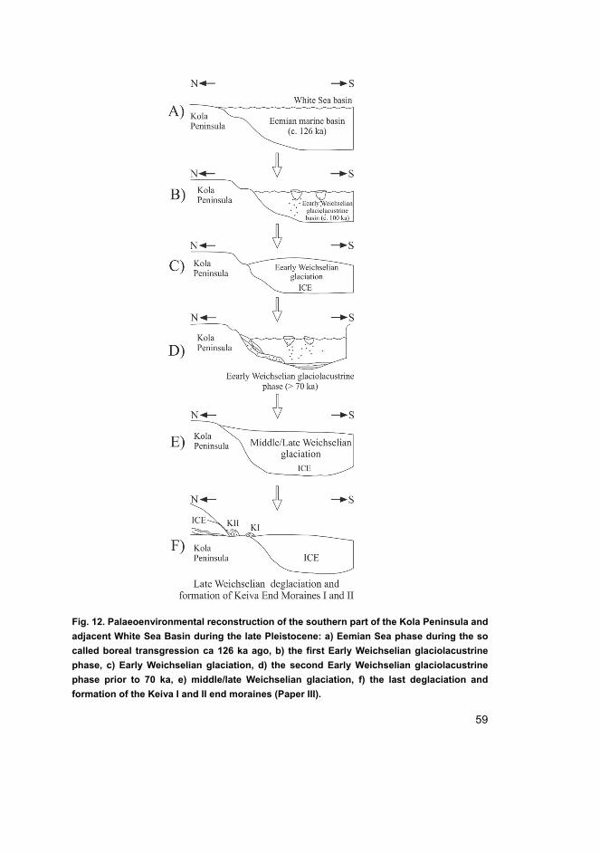
59

Fig. 12. Palaeoenvironmental reconstruction of the southern part of the Kola Peninsula and

adjacent White Sea Basin during the late Pleistocene: a) Eemian Sea phase during the so

called boreal transgression ca 126 ka ago, b) the first Early Weichselian glaciolacustrine

phase, c) Early Weichselian glaciation, d) the second Early Weichselian glaciolacustrine

phase prior to 70 ka, e) middle/late Weichselian glaciation, f) the last deglaciation and

formation of the Keiva I and II end moraines (Paper III).

60

stated (Krasnov et al. 1971, Ekman & Iljin 1991, Svendsen et. al. 2004, Hättestrand et al. 2007). It is also evident that it was in this interlobate zone into which Keiva I and II

moraines were deposited (Fig. 12F). Palaeocurrent data and geomorphological

observations show that melt water and sediment flow which formed the Keiva II end

moraine around Varzuga North, Strelna North, Pulonga North (i.e. sites that cut Keiva

II end moraine) was from NW to NE.Only one OSL sample was collected from Strelna

North delta (part of Keiva II) where foreset sand close to the topset facies yield an age

of ca. 12 ka suggesting that Keiva II end moraine was formed during the Younger Dryas

from the northeasterly direction. An OSL age from littoral sediments formed on the top

of glaciofluvial Keiva II subaquatic fan sediments in Varzuga East section yielded an

age of ca. 13.0 ka, which is also close to the Younger Dryas. Bottomset and foreset

sands dated from Varzuga East and North, however, range from ca. 20 ka to 61 ka and

these sands may not have been zeroed during sediment transportation. Based on the

obtained results, the Keiva II end moraine from the Varzuga area to at least as far as

Strelna River area was deposited mainly from sediment laden melt waters derived from

an ice mass located in the interior of the Kola Peninsula during the Younger Dryas.

Geomorphological evidence from Niemelä et al. (1993) together with our

observation suggest that sediments of the eastern part of Keiva II were derived from

the White Sea Ice lobe and the inland ice in the central part of Kola. The OSL-dating

results confirm the early assumptions of e.g. Vvedenski (1934), Lavrova (1960) and

Rainio et al. (1995) who suggested that the Keiva II end moraine is correlative with the

Salpausselkä end moraines in Finland. Keiva I end moraine complex is a discontinuous

suite of end moraine formations south of the Keiva II end moraine (Lunkka et al. 2001).

These formations include subaquatic fans composed of glaciofluvial sand and gravel

and also glaciotectonized push moraine ridges composed of till and deformed

sediments.

There are two sites in this study which are located at or adjacent to the Keiva I ice

marginal formations. Clast fabric measurements and glacitectonic structures from the

topmost till at the Strelna South site and the Babya site respectively indicate that ice

from the south overrode the area. According to OSL dates at Babya, the till unit

deposited during the last ice advance over the Babya area took place between 14.2 and

12.3 ka ago and related glaciofluvial subaquatic deposits were therefore deposited from

the south during the Younger Dryas. Based on the lithostratigraphic, palaeoflow,

glaciotectonic and OSL dating results, it is argued that the Keiva I end moraine at Babya

was deposited by the White Sea Ice lobe to the south at more or less the same time as

the Keiva II end moraine, which was deposited from the north. The palaeoflow and

dating results presented here confirm those assumptions made by Rainio et al. (1995)

61

and Svendsen et al. (2004) that both Keiva end moraines in the southern part of the

Kola Peninsula were deposited during the Younger Dryas in an intelobate zone of two

ice masses – one in the White Sea and the other in the interior of the Kola Peninsula.

Deltas, subaquatic fans, and silt-clay rhythmites indicate that glaciolacustrine basin(s)

were formed in the interlobate zone and later in the White Sea Basin as deglaciation

progressed (Pasanen et al. 2010, Putkinen et al., 2011, Lunkka et al. 2012).

Furthermore, the results indicate that the Keiva end moraines are correlative to the

Younger Dryas end moraine chain running around Fennoscandia as suggested by

Lundqvist & Saarnisto (1995).

7.4 Late Pleistocene Eurasian Arctic: importance of study and

future research

The Eurasian Arctic is still one of the most unexplored regions, although the many

expeditions and scientific observations were carried out recently due to the high

interest to the Arctic regions in last two decades. To improve our knowledge about

ice sheets development and depositional patterns in the Arctic region more local

areas need to be sampled and further investigated using complex of different

proxies. The results of this research will contribute towards the reconstruction of

palaeoenvironments, identification of source areas and transport pathways in the

Eurasian Arctic during the past 160 ka years.

Terrigenous components in Arctic Ocean surface sediments, including clay

minerals, bulk (light) minerals, and heavy minerals are the main source indicators

for provenance studies. In order to complete dataset using in this thesis the bulk

mineralogy can be used in future research, as bulk minerals including quartz,

feldspars, and detrital carbonates, are the most abundant minerals (besides clay

minerals) in Arctic Ocean sediments (Stein 2008). These data can be obtained using

X-ray diffraction analysis or microscopic analysis. According to Stein (2008), bulk

mineralogy X-ray diffraction data of Arctic Ocean sediments are still limited and

the additional data can shed light on the provenance determination.

The bulk mineralogy data is used also in quantitative provenance analysis

(QPA) that can be applied in the nearest future to samples from studied areas and

new locations. QPA is a useful tool for assessment of the types, amount and rates

of sediment supply from certain parental rock assemblages to a final sedimentary

depository (Weltje & von Eynatten 2004). QPA of late Pleistocene sediments

provide critical data for evaluation of possible pathways and source areas in the

Arctic regions. QPA results are especially useful tool for consideration deglaciation

62

and ice sheet disintegration and for discussion on ice rafting and inputs of melt

water as well as overall drainage distribution (Strand et al. 2017).

Data acquisition in QPA should include analysis of bulk mineralogy and

geochemical content and the selective analysis of a specific group of minerals, most

frequently heavy minerals as well as important varietal studies for geochemical and

possible radiometric signatures of single grains (Strand et al. 2017). Geochemical

or isotopic signals in single grains of a specific mineral can be used for provenance

studies in the nearest future due to the present increased availability of in-situ

micro-analytical techniques (Morton & Hallsworth 1994, 1999).

QPA can be applied to both terrestrial and marine sediments. On land setting

there is a critical to evaluate heavy mineral content of different diamict beds as a

possible indicator of a short term oscillation of the ice sheet. Glaciofluvial

reworking or glaciolacustrine intervals can be also determined using heavy mineral

content instead of just trying to determined major changes in directions of ice

streaming (Strand et al. 2017). The evaluation of sediment source for components

of crystalline rocks and a possible diagenesis of sediments in forming the complete

heavy mineral assemblages are a specific need in marine environments. Isotopic

and age characteristics of crystalline rocks in comparison with isotopic

characteristics of IRD from late Pleistocene ice-proximal sediments near to the

continental margins can be the useful approach.

63

8 Conclusions

The initial motivation for this research project was to assess the patterns and rates

of environmental changes during the past 160 000 years from the Late Saalian

glacial–Eemian interglacial to present in the Eurasian Arctic region. The results in

this thesis help to reconstruct interactions between components of the EurISs and

their development during the past 160 000 years using sedimentary sequences from

the central Arctic Ocean, SW Barents Sea and Kola Peninsula. The main

conclusions of the three included papers are:

– During the past 160 ka, four sediments sources, including Banks and Victoria

Islands with the MacKenzie River drainage, the Anabar massif, the Putorana

Plateau and the Verkhoyansk Fold Belt, provided most material to the

Lomonosov Ridge in the central Arctic Ocean in a varying range related to ice

sheet transitions (Publication I).

– The Amerasian sources supplied up to 80% of the material for the core site in

the central Arctic during transition MIS 6–5, and there was also a constant

Eurasian input of material from the Verkhoyansk Fold Belt. The input of

material from the North American margin during this transition suggests that

the eastern Eurasian margin and adjacent seas were covered by ice during this

time and only a small amount of material was supplied from Eurasian sources

by icebergs and calving sea ice (Publication I).

– The MIS 4–3 transition showed a change in sediment suppliers to the Eurasian

margin, and the most prominent sources were the Anabar massif and the

Putorana Plateau. A significant Eurasian input was related to rapid

sedimentation taking place at the study site. This event is associated with the

retreat of the BKIS and a possible input of Siberian hinterland ice-dammed

lake material into the Arctic Ocean (Publication I).

– In the SW Barents Sea, sediments were transported mainly from the Barents

Shelf and surrounding Barents Sea territories by a combination of glacial

erosion, iceberg calving, ocean currents and meltwater release during the last

deglaciation (Publication II).

– Sediments in the SW Barents Sea were divided into three lithostratigraphic

units. The lower Unit 3 is of glaciomarine origin, deposited in the environment

influenced by fluctuating influx of glacial melt-water; the genesis of Unit 2

varied in different locations, probably reflecting local ice–proximal

environments in cores BS231 and BS118 and an ice re-advance in core BS290;

64

and the upper Holocene Unit 1 represents open marine conditions (Publication

II).

– A mineralogical investigation of detrital grains from these units made it

possible to identify the sediment source areas. The SIS, BKIS, and BIS

behaved in a very dynamic way while disintegrating and multiple sources for

ice rafting material is more than evident in the SW Barents Sea. Besides

crystalline rock provenances, erosion products of the Mesozoic sediments at

the bottom of the Barents Sea are considered as a possible source of certain

heavy minerals being mixed with materials from the weathering crust of

Svalbard, the Fennoscandian Shield, and Franz Josef Land (Publication II).

– Investigation of the mineral contents of lower Unit 3 provides evidence that all

the surrounding Barents Sea territories could be possible source areas and a

most credible source is the Triassic sediments from the bottom of the Barents

Sea (Publication II).

– Unit 2 was deposited during an ice re-advance in the Bjørnøyrenna cross–shelf

trough and very local ice sheet proximity in Nordkappbanken bank.

Fennoscandia was the most important source area of mineralogical material

during this time for Nordkappbanken location. The Mesozoic sediments from

the bottom of Barents Sea are the most credible source for sediment deposited

in within Unit 2 in Bjørnøyrenna trough (Publication II).

– Unit 1 contains heavy minerals reworked from older sediments and clay

minerals deposited from the water column, partially transported by sea ice. The

presence of biogenic carbonates and smectite indicates warm Atlantic water

inflow (Publication II).

– The Eemian interglacial marine basin in the White Sea and the southern Kola

Peninsula changed gradually into a glaciolacustrine basin during the first part

of the Early Weichselian. Ice entered into the Varzuga area in the Early

Weichselian and subsequently retreated after which glaciolacustrine conditions

were re-established (Publication III).

– The second ice advance from the west into the Varzuga area occurred after 70

ka, most probably during the late Weichselian (Publication III).

– The last deglaciation of the southern and central coastal areas of the Kola

Peninsula took place between ca. 16 ka–12 ka. The eastern part of the Kola

Peninsula around Ponoy was deglaciated around 16 ka and the southern coastal

area from Varzuga area to Babya at around 12 ka (Publication III).

– The Keiva end moraines were deposited in an interlobate zone between the ice

mass in the interior of Kola and the White Sea ice lobe during the Younger

65

Dryas. The western part of the Keiva II end moraine (glaciofluvial deltas and

subaquatic fans) was laid down mainly from the north and the Keiva I end

moraines (glaciofluvial deltas and subaquatic fans) from the south (Publication

III).

66

67

List of references

Aagaard K, Swift JH & Carmack EC (1985) Thermohaline Circulation in the Arctic Mediterranean Seas. Journal of Geophysical Research 90 (C3): 4833–4846.

Aagaard K & Carmack EC (1994) The Arctic Ocean and climate: A perspective. In: Johannessen OM, Muench RD & Overland JE (ed) The Polar Oceans and Their Role in Shaping the Global Environment. Geophysical Monographs 85, American Geophysical Union: 5–20.

Adler RE, Polyak L, Ortiz JD, Kaufman DS, Channell JET, Xuan C, Grottoli AG, Sellen E & Crawford KA (2009) Sediment record from the western Arctic Ocean with an improved Late Quaternary age resolution: HOTRAX core HLY0503-8JPC, Mendeleev Ridge. Global Planetary Change 68: 18–29.

Alexanderson H, Hjort C, Moller P, Antonov O & Pavlov M (2001) The North Taymyr ice-marginal zone, Arctic Siberia—A preliminary overview and dating, Global Planetary Change 31(1–4): 427–446.

Andreassen K, Laberg JS & Vorren T (2008) Seafloor geomorphology of the SW Barents Sea and its glaci–dynamic implications. Geomorphology 97: 157–177.

Andrews JT (1971) Techniques of Till Fabric Analysis. Technical Bulletin No. 6. British Geomorphological Research Group.

AMAP (1998) AMAP Assessment Report: Arctic Pollution Issues. Arctic Monitoring and Assessment Programme (AMAP). Oslo, Norway.

Apukhtin NI (1978) New data on Quaternary stratigraphy of the southeastern part of the Kola Peninsula. Proceedings of VSEGEI Leningrad. Quaternary geology and geoorphology 297: 53–65 (in Russian).

Armand AD & Lebedeva RM (1966) Sporovo-pyltsevaya kharakteristika opornogo razreza mezhlednikovykh otlozhenii na yuzhnom beregu Kol’skogo poluostrova (Spore-and-pollen characteristic of the key section of Interglacial deposits in the southern coastal area of the Kola Peninsula). In: Formirovanie reliefa i chetvertichnykh otlozhenii Kol’skogo poluostrova (In: The topography and Quaternary deposits formation of the Kola Peninsula). Nauka, Moscow-Leningrad: 77–86 (in Russian).

Astakhov V (2004) Middle Pleistocene glaciations of the Russian North. Quaternary Science Reviews 23: 1285–1311.

Backman J & Moran K (2009) Expanding the Cenozoic paleoceanographic record in the Centaral Arctic Ocean: IODP Expedition 302 Synthesis. Central European Journal of Geosciences 1: 157–175.

Bassinot FC, Labeyrie LD, Vincent E, Qudelleur X, Shackleton NJ & Lancelot Y (1994) The astronomical theory of climate and the age of the Brunhes-Matuyama magnetic reversal. Earth and Planetary Science Letters 126: 91–108.

Berglund B. & Ralska-Jasiewiczowa M (1990) Pollen analysis and pollen diagrams. In: Berglund BE (ed) Handbook of Holocene Palaeoecology and Palaeohydrology. J. Wiley & Sons, Chichester: 455–484.

Biscaye PF (1964) Distinction between kaolinite and chlorite in recent sediments by X–ray diffraction. American Mineralogist 49: 1281–1289.

68

Biscaye PF (1965) Mineralogy and sedimentation of recent deep–sea clay in the Atlantic Ocean and adjacent seas and oceans. Geological Society of America Bulletin 76: 803–832.

Bischof JF, Clark DL & Vincent J-S (1996) Origin of ice-rafted debris: Pleistocene paleoceanography in the western Arctic Ocean. Paleoceanography 11: 743–756.

Bischof JF & Darby D (1997) Mid- to late pleistocene ice drift in the western Arctic Ocean: evidence for a different circulation in the past. Science 277: 74–78.

Björk G, Jakobsson M, Rudels B, Swift JH, Anderson L, Darby DA, Backman J, Coakley B, Winsor P, Polyak L & Edwards M (2007) Bathymetry and deep-water exchange across the Lomonosov Ridge at 88°-89°N. Deep-Sea Research I-54: 1197–1208.

Bøtter-Jensen L. Bulur E, Duller GAT & Murray AS (2000) Advances in luminescence instrument systems. Radiation Measurements 32: 523–528.

Brozena JM, Childers VA, Lawver LA, Gahagan LM, Forsberg R, Faleide JI & Eldholm O (2003) New aerogeophysical study of the Eurasia Basin and Lomonosov Ridge: Implications for basin development. Geology 31(9): 825–828.

Bugge T, Mangerud G, Elvebakk G, Mørk A, Nilsson I, Fanavoll S & Vigran JO (1995) The Upper Palaeozoic succession on the Finnmark Platform, Barents Sea. Norsk Geologisk Tidsskrift 75: 3–30.

Cheremisinova EA (1962) Diatoms from the Kola Peninsula marine interglacial deposits (Diatomovaya flora morskih mezhlednikovyh otlozhenii Kolskogo poluostrova). Proceeding of geology and mineral deposits of the northwest RSFSR (Materialy po geologii I poleznym iskopaemum severo-zapada RSFSR) 3: 45–57.

Cohen KM, Finney SC, Gibbard PL & Fan J-X (2013) The ICS International Chronostratigraphic Chart. Episodes 36: 199–204.

Comiso JC, Parkinson CL, Gersten R & Stock L (2008) Accelerated decline in the Arctic sea ice cover. Geophysical Research Letters 35: L01703.

Dahlgren KIT, Vorren TO, Stoker MS, Nielsen T, Nygård A & Sejrup HP (2005) Late Cenozoic prograding wedges on the NW European margin: their formation and relationship to tectonics and climate. Marine and Petroleum Geology 22: 1089–1110.

Demidov L, Houmark-Nielsen M Kjær KH & Larsen E (2006) The last Scandinavian ice sheet in northwestern Russia: ice flow patterns and decay dynamics. Boreas 35-3: 425–443.

Doré AG (1995) Barents Sea Geology, Petroleum Resources and Commercial Potential. Arctic 48: 207–221.

Ehlers J & Gibbard PL (2003) Extent and chronology of glaciations. Quaternary Science Review 22: 1561–1568.

Ehlers J & Gibbard PL (2007) The extent and chronology of Cenozoic global glaciation. Quaternary International 164–165: 6–20.

Eidvin T, Jansen E & Riis F (1993) Chronology of Tertiary fan deposits off the western Barents Sea: implications for the uplift and erosion history of the Barents Shelf. Marine Geology 112: 109–131.

69

Eidvin T, Goll RM, Grogan P, Smelror M & Ulleberg K (1998) The Pleistocene to Middle Eocene stratigraphy and geological evolution of the western Barents Sea continental margin at well site 7316/5–1 (Bjørnøya West area). Norsk Geologisk Tidsskrift 78: 99–123.

Ekman I & Iljin V (1991) Deglaciation, the Younger Dryas end moraines and their correlation in the Karelian A.S.S.R. and adjacent areas. In: Rainio H & Saarnisto M (eds) Eastern Fennoscandian Younger Dryas and moraines – Excursion Guide. IGCP Project 253, Termination of Pleistocene. Geological Survey of Finland, Espoo, Finland: 73–102.

Elverhøi A, Fjeldskaar W, Solheim A, Nyland–Berg M & Russwurm L (1993) The Barents Sea Ice Sheet — a model of its growth and decay during the last ice maximum. Quaternary Science Reviews 12: 863–873.

Emiliani C (1955) Pleistocene temperatures. The Journal of Geology 63: 538–578. Eyles N (1983) Glacial Geology: A Landsystem Approach. In: Eyles N (ed) Glacial Geology:

An Introduction for Engineers and Earth Scientists. Pergamon Press, Oxford-New York: 1–18.

Faegri K & Iversen J (1989) Textbook of pollen analyses (4th edition, revised by Faegri K, Kaland P. & Krzywinski K). John Wiley, Chichester.

Fagel N, Not C, Gueibe J, Mattielli N & Bazhenova E (2014) Late Quaternary evolution of sediment provenances in the Central Arctic Ocean: mineral assemblage, trace element composition and Nd and Pb isotope fingerprints of detrital fraction from the Northern Mendeleev Ridge. Quaternary Science Reviews 92: 140–154.

Faleide JI, Solheim A, Fiedler A, Hjelstuen BO, Andersen ES & Vanneste K (1996) Late Cenozoic evolution of the western Barents Sea–Svalbard continental margin. In: Solheim A (ed): Impact of Glaciations on Basin Evolution: Data and Models from the Norwegian Margin and Adjacent Areas. Global and Planetary Change 12: 53–74.

Folk RL (1980) Petrology of Sedimentary Rocks. Hemphill Publishing Company. Goslar T, Czernik J & Goslar E (2004) Low-energy 14C AMS in Poznań Radiocarbon

Laboratory, Poland. Nuclear Instruments and Methods in Physics Research Section B: Beam Interactions with Materials and Atoms 223–224: 5–11.

Grave MK, Gunova VS, Devyatova EI, Lavrova MA, Lebedeva RM, Samsonova LYa & Cheremisinova EA (1969) Mikulino interglacial in southeast of the Kola Peninsula. In: Osnovnye problemy geomorfologii i stratigrafii antropogena Kolskogo poluostrova (In: Main problems of geomorphology and stratigraphy of the Quaternary at the Kola Peninsula). Leningrad: 25–56 (in Russian).

Grimm E (1991) Tilia 1.12, Tilia Graph 1.18. Springfield, Illinois State Museum, Research and Collection Center.

Gudlaugsson ST, Faleide JI, Johansen SE & Breivik AJ (1998) Late Palaeozoic structural development of the South–Western Barents Sea. Marine and Petroleum Geology 15: 73– 102.

Hald M & Vorren TO (1987) Foraminiferal stratigraphy and environment of Late Weichselian deposits on the continental shelf off Troms, Northern Norway. Marine Micropalaeontology 12: 129–160.

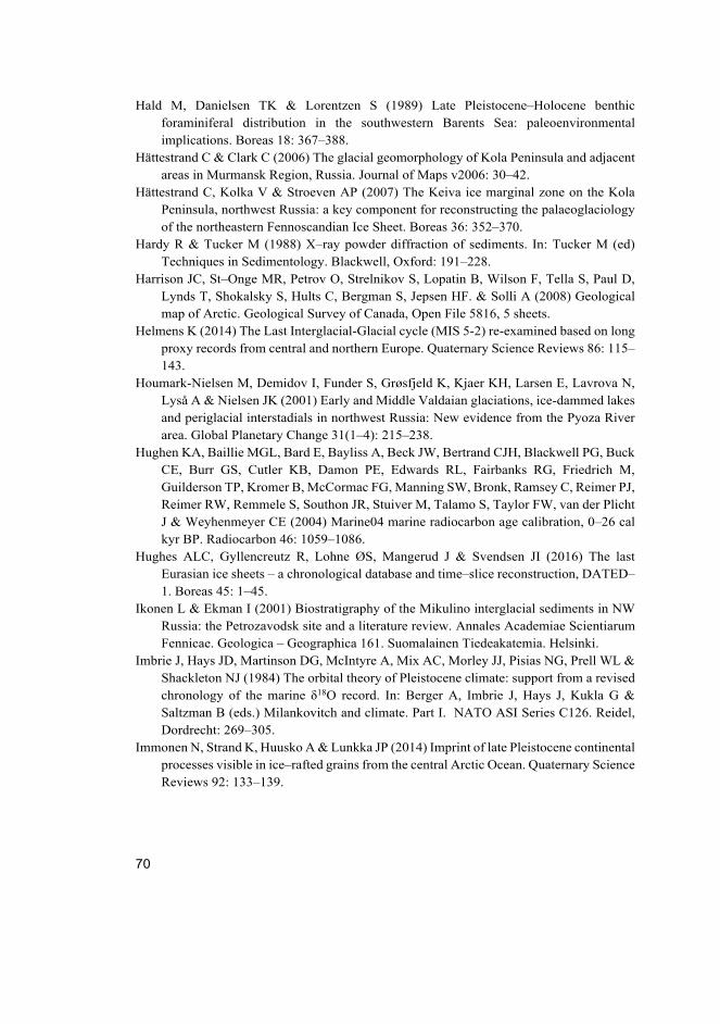
70

Hald M, Danielsen TK & Lorentzen S (1989) Late Pleistocene–Holocene benthic foraminiferal distribution in the southwestern Barents Sea: paleoenvironmental implications. Boreas 18: 367–388.

Hättestrand C & Clark C (2006) The glacial geomorphology of Kola Peninsula and adjacent areas in Murmansk Region, Russia. Journal of Maps v2006: 30–42.

Hättestrand C, Kolka V & Stroeven AP (2007) The Keiva ice marginal zone on the Kola Peninsula, northwest Russia: a key component for reconstructing the palaeoglaciology of the northeastern Fennoscandian Ice Sheet. Boreas 36: 352–370.

Hardy R & Tucker M (1988) X–ray powder diffraction of sediments. In: Tucker M (ed) Techniques in Sedimentology. Blackwell, Oxford: 191–228.

Harrison JC, St–Onge MR, Petrov O, Strelnikov S, Lopatin B, Wilson F, Tella S, Paul D, Lynds T, Shokalsky S, Hults C, Bergman S, Jepsen HF. & Solli A (2008) Geological map of Arctic. Geological Survey of Canada, Open File 5816, 5 sheets.

Helmens K (2014) The Last Interglacial-Glacial cycle (MIS 5-2) re-examined based on long proxy records from central and northern Europe. Quaternary Science Reviews 86: 115–143.

Houmark-Nielsen M, Demidov I, Funder S, Grøsfjeld K, Kjaer KH, Larsen E, Lavrova N, Lyså A & Nielsen JK (2001) Early and Middle Valdaian glaciations, ice-dammed lakes and periglacial interstadials in northwest Russia: New evidence from the Pyoza River area. Global Planetary Change 31(1–4): 215–238.

Hughen KA, Baillie MGL, Bard E, Bayliss A, Beck JW, Bertrand CJH, Blackwell PG, Buck CE, Burr GS, Cutler KB, Damon PE, Edwards RL, Fairbanks RG, Friedrich M, Guilderson TP, Kromer B, McCormac FG, Manning SW, Bronk, Ramsey C, Reimer PJ, Reimer RW, Remmele S, Southon JR, Stuiver M, Talamo S, Taylor FW, van der Plicht J & Weyhenmeyer CE (2004) Marine04 marine radiocarbon age calibration, 0–26 cal kyr BP. Radiocarbon 46: 1059–1086.

Hughes ALC, Gyllencreutz R, Lohne ØS, Mangerud J & Svendsen JI (2016) The last Eurasian ice sheets – a chronological database and time–slice reconstruction, DATED–1. Boreas 45: 1–45.

Ikonen L & Ekman I (2001) Biostratigraphy of the Mikulino interglacial sediments in NW Russia: the Petrozavodsk site and a literature review. Annales Academiae Scientiarum Fennicae. Geologica – Geographica 161. Suomalainen Tiedeakatemia. Helsinki.

Imbrie J, Hays JD, Martinson DG, McIntyre A, Mix AC, Morley JJ, Pisias NG, Prell WL & Shackleton NJ (1984) The orbital theory of Pleistocene climate: support from a revised chronology of the marine δ18O record. In: Berger A, Imbrie J, Hays J, Kukla G & Saltzman B (eds.) Milankovitch and climate. Part I. NATO ASI Series C126. Reidel, Dordrecht: 269–305.

Immonen N, Strand K, Huusko A & Lunkka JP (2014) Imprint of late Pleistocene continental processes visible in ice–rafted grains from the central Arctic Ocean. Quaternary Science Reviews 92: 133–139.

71

IPCC (2014) Climate Change 2014: Synthesis Report. Contribution of Working Groups I, II and III to the Fifth Assessment Report of the Intergovernmental Panel on Climate Change (Core Writing Team Pachauri RK & Meyer LA (eds)). IPCC, Geneva, Switzerland.

Jakobsson M, Løvlie R, Al-Hanbali H, Arnold E, Backman J & Mörth M (2000) Manganese and color cycles in Arctic Ocean sediments constrain Pleistocene chronology. Geology 28: 23–26.

Jakobsson M, Løvlie R, Arnold EM, Backman J, Polyak L, Knutsen, J-O & Musatov E (2001) Pleistocene stratigraphy and paleoenvironmental variation from Lomonosov Ridge sediments, central Arctic Ocean. Global and Planetary Change 31: 1–22.

Jakobsson M (2002) Hypsometry and volume of the Arctic Ocean and its constituent seas. Geochemistry, Geophysics, Geosystems 3: 1–18.

Jakobsson M, Backman J, Murray A & Løvlie R (2003) Optically simulated luminescence dating support central Arctic Ocean cm-scale sedimentation rates. Geochemistry Geophysics Geosystems 4: 1–11.

Jakobsson M, Macnab R, Mayer M, Anderson R, Edwards M, Hatzky J, Schenke H-W & Johnson P (2008) An improved bathymetric portrayal of the Arctic Ocean: Implications for ocean modeling and geological, geophysical and oceanographic analyses. Geophysical Research Letters 35: LO7602.

Jakobsson M, Mayer LA, Coakley B, Dowdeswell JA & Forbes S (2012) The International Bathymetric Chart of the Arctic Ocean (IBCAO) version 3.0. Geophysical Research Letters 39: L12609.

Jakobsson M, Nilsson J, Anderson L, Backman J, Björk G, Cronin TM, Kirchner N, Koshurnikov A, Mayer L, Noormets R, O’Regan M, Stranne C, Ananiev R, Macho NB, Chernykh D, Coxall HK, Eriksson B, Flodén T, Gemery L, Gustafsson Ö, Jerram K, Johansson C, Khortov A, Mohammad R & Semiletov I (2016) Evidence for an ice shelf covering the central Arctic Ocean during the penultimate glaciations. Nature Communications 7: 1–10.

Jokat W, Uenzelmann-Neben G, Kristoffersen Y & Rasmussen T (1992) ARCTIC’91: Lomonosov Ridge – a double sided continental margin. Geology 20: 887–890.

Junttila J, Aagaard–Sørensen S, Husum K & Hald M (2010) Late Glacial–Holocene clay minerals elucidating glacial history in the SW Barents Sea. Marine Geology 276: 71–85.

Koistinen T, Stephens MB, Bogatchev V, Nordgulen Ø, Wennerström M & Korhonen J (2001) Geological map of the Fennoscandian Shield, scale 1:2 000 000. Espoo, Geological Survey of Finland; Geological Survey of Norway, Trondheim; Geological Survey of Sweden, Uppsala; Ministry of Natural Resources of Russia, Moscow.

Krasnov II, Duphorn K & Voges A (1971) International Quaternary Map of Europe, Sheet 3: Nordkapp. INQUA Commission. Hannover, Bundesanstalt für Bodenforschung.

Krylov AA, Andreeva IA, Vogt C, Backman J, Krupskaya VV, Grikurov GE, Moran K & Shoji H (2008) A shift in heavy and clay mineral provenance indicates a middle Miocene onset of a perennial sea ice cover in the Arctic Ocean. Paleoceanography 23: PA1S06.

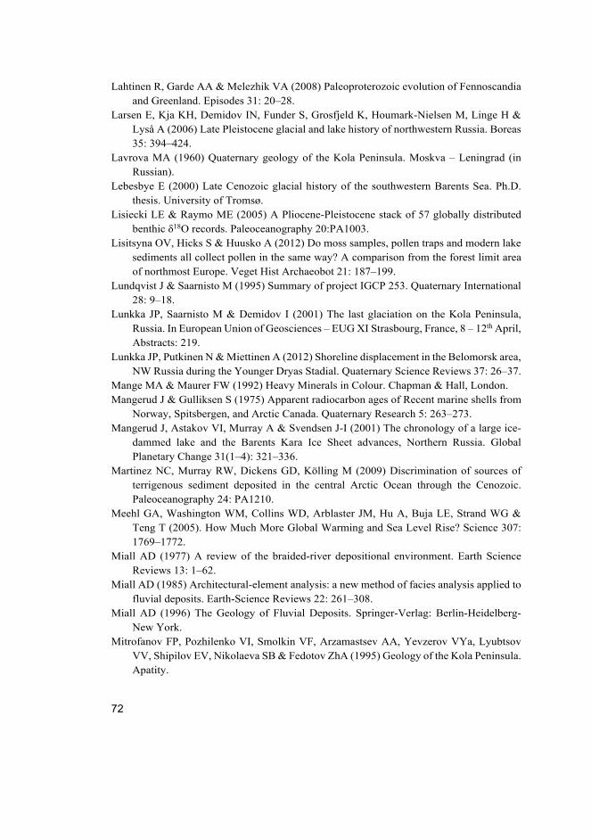
72

Lahtinen R, Garde AA & Melezhik VA (2008) Paleoproterozoic evolution of Fennoscandia and Greenland. Episodes 31: 20–28.

Larsen E, Kja KH, Demidov IN, Funder S, Grosfjeld K, Houmark-Nielsen M, Linge H & Lyså A (2006) Late Pleistocene glacial and lake history of northwestern Russia. Boreas 35: 394–424.

Lavrova MA (1960) Quaternary geology of the Kola Peninsula. Moskva – Leningrad (in Russian).

Lebesbye E (2000) Late Cenozoic glacial history of the southwestern Barents Sea. Ph.D. thesis. University of Tromsø.

Lisiecki LE & Raymo ME (2005) A Pliocene-Pleistocene stack of 57 globally distributed benthic δ18O records. Paleoceanography 20:PA1003.

Lisitsyna OV, Hicks S & Huusko A (2012) Do moss samples, pollen traps and modern lake sediments all collect pollen in the same way? A comparison from the forest limit area of northmost Europe. Veget Hist Archaeobot 21: 187–199.

Lundqvist J & Saarnisto M (1995) Summary of project IGCP 253. Quaternary International 28: 9–18.

Lunkka JP, Saarnisto M & Demidov I (2001) The last glaciation on the Kola Peninsula, Russia. In European Union of Geosciences – EUG XI Strasbourg, France, 8 – 12th April, Abstracts: 219.

Lunkka JP, Putkinen N & Miettinen A (2012) Shoreline displacement in the Belomorsk area, NW Russia during the Younger Dryas Stadial. Quaternary Science Reviews 37: 26–37.

Mange MA & Maurer FW (1992) Heavy Minerals in Colour. Chapman & Hall, London. Mangerud J & Gulliksen S (1975) Apparent radiocarbon ages of Recent marine shells from

Norway, Spitsbergen, and Arctic Canada. Quaternary Research 5: 263–273. Mangerud J, Astakov VI, Murray A & Svendsen J-I (2001) The chronology of a large ice-

dammed lake and the Barents Kara Ice Sheet advances, Northern Russia. Global Planetary Change 31(1–4): 321–336.

Martinez NC, Murray RW, Dickens GD, Kölling M (2009) Discrimination of sources of terrigenous sediment deposited in the central Arctic Ocean through the Cenozoic. Paleoceanography 24: PA1210.

Meehl GA, Washington WM, Collins WD, Arblaster JM, Hu A, Buja LE, Strand WG & Teng T (2005). How Much More Global Warming and Sea Level Rise? Science 307: 1769–1772.

Miall AD (1977) A review of the braided-river depositional environment. Earth Science Reviews 13: 1–62.

Miall AD (1985) Architectural-element analysis: a new method of facies analysis applied to fluvial deposits. Earth-Science Reviews 22: 261–308.

Miall AD (1996) The Geology of Fluvial Deposits. Springer-Verlag: Berlin-Heidelberg-New York.

Mitrofanov FP, Pozhilenko VI, Smolkin VF, Arzamastsev AA, Yevzerov VYa, Lyubtsov VV, Shipilov EV, Nikolaeva SB & Fedotov ZhA (1995) Geology of the Kola Peninsula. Apatity.

73

Moore DM & Reynolds RC (1997) X–ray Diffraction and the Identification and Analysis of Clay Minerals (2nd edition). Oxford University Press, Oxford.

Moore PD, Webb JA & Collinson ME (1991) Pollen analysis (2nd edition). Blackwell, Oxford.

Morton AC & Hallsworth CR (1994) Identifying provenance–specific features of detrital heavy mineral assemblages in sandstones. Sedimentary Geology 90: 241–256.

Morton AC & Hallsworth CR (1999) Processes controlling the composition of heavy mineral assemblages in sandstones. Sedimentary Geology 124: 3–29.

Mueller DR, Vincent WF & Jeffries MO (2003) Break-up of the largest Arctic ice shelf and associated loss of an epishelf lake. Geophysical Research Letters 30(20): 2031.

Murdmaa I, Ivanova E, Duplessy J–C, Levitan M, Khusid T, Bourtman M, Alekhina G, Alekseeva T, Belousov M & Serova V (2006) Facies system of the Eastern Barents Sea since the last glaciation to present. Marine Geology 230: 275–303.

Murray AS, Marten R, Johnston A & Martin P (1987) Analysis for naturally occurring radionuclides at environmental concentrations by gamma spectrometry. Journal of Radioanalytical and Nuclear Chemistry 115: 263–288.

Murray AS & Olley JM (1999) Determining sedimentation rates using luminescence dating. In: Bruns P & Hass HC (eds) Determination of Sedimentation Accumulation Rates. GeoResearch Forum 5, Trans Tech Publ., Switzerland: 121–144.

Murray AS & Wintle AG (2000) Luminescence dating of quartz using an improved single-aliquot regenerative-dose protocol. Radiation measurements 32: 57–73.

Murray AS & Olley JM (2002) Precision and accuracy in the optically stimulated luminescence dating of sedimentary quartz: A status review. Geochronometrica 21: 1–15.

Murray AS & Wintle AG (2003) The single aliquot regenerative dose protocol: potential for improvements in reliability. Radiation Measurements 37(4-5): 377– 381.

Niemelä J, Lukashov A & Ekman I (1993) Quaternary deposits of Finland and northwestern part of Russian Federation and their resources. Map 1: 1 000 000, Sheet 2. Geological Survey of Finland & Institute of Geology at the Karelian Science Centre of the Russian Academy of Sciences: Espoo.

Not C & Hillaire-Marcel C (2012) Enhanced sea-ice export from the Arctic during the Younger Dryas. Nat. Commun. 3: 647.

Olley JM, Murray AS & Roberts RG (1996) The effects of disequilibria in the uranium and thorium decay chains on burial dose rates in fluvial sediments. Quaternary Science Reviews 15: 751–760.

Pasanen A, Lunkka JP & Putkinen N (2010) Reconstruction of the White Sea Basin during the late Younger Dryas. Boreas 39: 273–285.

Prescott JR & Hutton JT (1994) Cosmic ray contributions to dose-rates for luminescence and ESR dating: large depths and long-term time variations. Radiation Measurements 23(2/3): 497–500.

Putkinen N, Lunkka JP, Ojala AEK & Kosonen E (2011) Deglaciation history and age estimate of the Younger Dryas end moraines in the Kalevala region, NW Russia. Quaternary Science Reviews 30: 3812–3822.

74

Rainio H, Saarnisto M & Ekman I (1995) Younger Dryas end moraines in Finland and NW Russia. Quaternary International 28: 179–192.

Reille M (1992) Pollen et spores d’Europe et d’Afrique du nord. Laboratoire de botanique historique et palynologie, Marseille.

Reimer PJ & Reimer RW (2001) A marine reservoir correction database and on–line interface. Radiocarbon 43: 461–463.

Reimer PJ, Baillie MGL, Bard E, Bayliss A, Beck JW, Bertrand CJH, Blackwell PG, Buck CE, Burr GS, Cutler KB, Damon PE, Edwards RL, Fairbanks RG, Friedrich M, Guilderson TP, Hogg AG, Hughen KA, Kromer B, McCormac G, Manning S, Ramsey CB, Reimer RW, Remmele S, Southon JR, Stuiver M, Talamo S, Taylor FW, van der Plicht J & Weyhenmeyer CE (2004) IntCal04 Terrestrial radiocarbon age calibration, 26–0 ka BP. Radiocarbon 46: 1029–1058.

Riis F (1996) Quantification of Cenozoic vertical movements of Scandinavia by correlation of morphological surfaces with offshore data. Global and Planetary Change 12: 331–357.

Rüther DC, Mattingsdal R, Andreassen K, Forwick M & Husum K (2011) Seismic architecture and sedimentology of a major grounding zone system deposited by the Bjørnøyrenna Ice Stream during late Weichselian deglaciation. Quaternary Science Reviews 30: 2776–2792.

Rüther DC, Bjarnadóttir LR, Junttila J, Husum K, Rasmussen TL, Lucchi RG & Andreassen K (2012) Pattern and timing of the northwestern Barents Sea Ice Sheet deglaciation and indications of episodic Holocene deposition. Boreas 41–3: 494–512.

Sakshaug E & Skjoldal HR (1989) Life at the ice edge. Ambio 18 (1): 60–67. Sættem J, Bugge T, Fanavoll S, Goll RM, Mørk A, Mørk MBE, Smelror M & Verdenius JG

(1994) Cenozoic margin development and erosion of the Barents Sea: core evidence from southeast Bjørnøya. Marine Geology 118: 257–281.

Schoster F, Behrends M, Müller C, Stein R & Wahsner M (2000) Modern river discharge and pathways of supplied material in the Eurasian Arctic Ocean: evidence from mineral assemblages and major and minor element distribution. Int. J. Earth Sci. 89: 486–495.

Sejrup HP, Larsen E, Haflidason H, Berstad IM, Hjelstuen BO, Jonsdottir H, King EL, Landvik J, Longva O, Nygard A, Ottesen D, Raunholm S, Rise L & Stalsberg K (2003) Configuration, history and impact of the Norwegian Channel Ice Stream. Boreas 32: 18–36.

Sellén E (2009) Quaternary paleoceanography of the Arctic Ocean: A study of sediment stratigraphy and physical properties. Ph.D. thesis. Stockholm University, Department of Geology and Geochemistry.

Shackleton NJ, Sánchez-Goñi MF, Pailler D & Lancelot Y (2003) Marine Isotope Substage 5e and the Eemian Interglacial. Global and Planetary Change 36: 151–155.

Siedlecka A & Roberts D (1996) Finnmark country. Bedrock geology. Scale 1:500000. Norges geologiske undersøkelse.

Sigmond EMO (1992) Bedrock map. Norway and adjacent ocean areas. Scale 1:3 million. Geological Survey of Norway.

75

Sigmond EMO (2002) Geological map. Land and sea areas of northern Europe. Scale 1:4 million. Norges geologiske undersøkelse.

Ślubowska–Woldengen M, Koç N, Rasmussen TL, Klitgaard–Kristensen D, Hald M & Jennings AE (2008) Time–slice reconstructions of ocean circulation changes on the continental shelf in the Nordic and Barents Seas during the last 16,000 cal yr B.P. Quaternary Science Reviews 27: 1476–1492.

Smith DGW & Higgins MD (2003) MinIdent for Windows, version 3.00 Professional, database 1.0. Canadian Mineralogist 41: 548–552.

Spielhagen RF, Baumann K-H, Erlenkeuser H, Nowaczyk NR, Norgaard-Pedesen N, Vogt C & Weiel D (2004) Arctic Ocean deep-sea record of northern Eurasian ice sheet history. Quaternary Science Reviews 23: 1455–1483.

Stein R (2008) Arctic Ocean sediments: proxies, and paleoenvironment. Volume 2, 1st edition. Developments in Marine Geology, Elsevier Science.

Strand K, Kaparulina E, Immonen N, Junttila J, Lunkka JP & Sarala P (2017) Quantitative provenance analysis implications for late Pleistocene deglaciations on land and marine setting (abstract). 5th International Conference on Palaeo-Arctic Spatial and Temporal (PAST) Gateways: 29–30.

Strelkov SA, Yevzerov VYa & Koshechkin BI (1976) The history of formation of the relief and loose deposits of the northeastern Baltic Shield. Leningrad (In Russian).

Svendsen JI, Astakhov VI, Bolshiyanov DY, Demidov I, Dowdeswell JA, Gataullin V, Hjort C, Hubberten HW, Larsen E, Mangerud J, Melles M, Möller P, Saarnisto M & Siegert MJ (1999) Maximum extent of the Eurasian ice sheets in the Barents and Kara Sea region during the Weichselian. Boreas 28: 234–242.

Svendsen JI, Alexanderson H, Astakhov VI, Demidov I, Dowdeswell JA, Funder S, Gataullin V, Henriksen M, Hjort C, Houmark-Nielsen M, Hubberten HW, Ingólfson Ó, Jakobsson M, Kjær KH, Larsen E, Lokrantz H, Lunkka JP, Lyså A, Mangerud J, Matiouchkov A, Murray A, Möller P, Niessen F, Nikolskaya O, Polyak L, Saarnisto M, Siegert C, Siegert MJ, Spielhagen RF & Stein R (2004) Late Quaternary ice sheet history of northern Eurasia. Quaternary Science Reviews 23: 1229–1271.

Svendsen JI, Krüger LC, Mangerud J, Astakhov VI, Paus A, Nazarov D & Murray A (2014) Glacial and vegetation history of the Polar Ural Mountains in northern Russia during the Last Ice Age, Marine isotope stages 5 – 2. Quaternary Science Reviews 92: 409–428.

Thomsen E & Vorren TO (1987) Macrofaunal paleoecology and stratigraphy in late Quaternary shelf sediments off Northern Norway. Paleogeography, Paleoclimatology, Paleoecology 56: 103–150.

Vassmyr S & Vorren TO (1990) Clast petrography and stratigraphy in Late Quaternary sediments in the southwestern Barents Sea. Norsk Geologisk Tidsskrift 70: 95–110.

Vogt PR, Taylor PT, Kovacs LC & Johnson GL (1979) Detailed aeromagnetic investigation of the Arctic Basin. Journal of Geophysical Research 84: 1071–1089.

Vogt C & Knies J (2009) Sediment pathways in the western Barents Sea inferred from clay mineral assemblages in surface sediments. Norwegian Journal of Geology 89: 41–55.

76

Vorren TO, Hald M & Thomsen E (1984) Quaternary sediments and environments on the continental shelf off Northern Norway. Marine Geology 57: 229–257

Vorren TO, Hald M & Lebesbye E (1988) Late Cenozoic environments in the Barents Sea. Paleoceanography 3: 601–612.

Vorren TO & Laberg JS (1996) Late Glacial air temperature, oceanographic and ice sheet interactions in the southern Barents Sea region. In: Andrews JT, Austin WEN, Bergsten H & Jennings AE (eds) Late Quaternary Palaeoceanography of the North Atlantic Margins. Geological Society Special Publication 11: 303–321.

Vorren TO & Laberg JS (1997) Trough mouth fans — palaeoclimate and ice sheet monitors. Quaternary Science Reviews 16: 865–881.

Vorren TO, Laberg JS, Blaume F, Dowdeswell JA, Kenyon N, Mienert J, Rumohr J & Werner F (1998) The Norwegian–Greenland Sea continental margins: morphology and Late Quaternary process and environment. Quaternary Science Reviews 17: 273–302.

Vvedenski LV (1934) Reljef yuzhnoi chasti Kolskogo poluostrova (Relief of the southern part of the Kola Peninsula). Izvestiya geographicheskogo obshestva SSSR (Proceedings of the geographical society of the USSR) LXVI (6): 844–863.

Wallinga J, Murray AS, Wintle AG & Bøtter-Jensen L (2002) Measurement of the dose in quartz in the presence of feldspar contamination. Radiation Protection Dosimetry 101 (1-4): 367–370.

Weltje GF & von Eynatten H (2004) Quantitative provenance analysis of sediments: review and outlook. Sedimentary Geology 171: 1–11.

Wilson JT (1963) Hypothesis of earth’s behavior. Nature 198: 925–929. Winsborrow MCM, Andreassen K, Corner GD & Laberg JS (2010) Deglaciation of a

marine–based ice sheet: Late Weichselian palaeo–ice dynamics and retreat in the southern Barents Sea reconstructed from onshore and offshore glacial geomorphology. Quaternary Science Reviews 29: 424–442.

Yakubchuk AS & Nikishin AM (2005) Russia. In: Selley RC, Cocks LRM, Plimer IR (ed) Encyclopedia of Geology 4. Elsevier, Amsterdam: 456–473.

Yevzerov VYa & Koshechkin BI (1980) Paleogeography of the Pleistocene of the western Kola Peninsula. Leningrad (In Russian).

Zachos J, Pagani M, Sloan L, Thomas E & Billups K (2001) Trends, Rhythms, and Aberrations in Global Climate: 65 Ma to Present. Science 292: 686–693.

77

Original publications

I Kaparulina E, Strand K & Lunkka JP (2016) Provenance Analysis of Central Arctic Ocean Sediments: Implications for Circum-Arctic Ice Sheet Dynamics and Ocean Circulation during Late Pleistocene. Quaternary Science Reviews 147: 210–220.

II Kaparulina E, Junttila J, Strand K, & Lunkka JP (2017) Provenance Signatures and Changes of the Southwestern Sector of the Barents Ice Sheet during the Last Deglaciation. Boreas. doi:10.1111/bor.12293. ISSN 0300-9483.

III Lunkka JP, Kaparulina E, Putkinen N & Saarnisto M (2017) Late Pleistocene Paleoenvironments and the Last Deglaciation on the Kola Peninsula, Russia. Manuscript.

Reprinted with permission from Elsevier (Article I) and Boreas (Article II).

Original publications are not included in the electronic version of the dissertation.

78

A C T A U N I V E R S I T A T I S O U L U E N S I S

Book orders:Granum: Virtual book storehttp://granum.uta.fi/granum/

S E R I E S C T E C H N I C A

626. Lappi, Tuomas (2017) Formation and governance of a healthy business ecosystem

627. Samarakoon, Sumudu (2017) Learning-based methods for resource allocation andinterference management in energy-efficient small cell networks

628. Pargar, Farzad (2017) Resource optimization techniques in scheduling :applications to production and maintenance systems

629. Uusitalo, Pauliina (2017) The bound states in the quantum waveguides of shape Y,Z, and C

630. Palosaari, Jaakko (2017) Energy harvesting from walking using piezoelectriccymbal and diaphragm type structures

631. Mononen, Petri (2017) Socio-economic impacts of a public agency – enhancingdecision support for performance management

632. Kärkkäinen, Marja-Liisa (2017) Deactivation of oxidation catalysts by sulphur andphosphorus in diesel and gas driven vehicles

633. Viittala, Harri (2017) Selected methods for WBAN communications — FM-UWBand SmartBAN PHY

634. Akram, Saad Ullah (2017) Cell segmentation and tracking via proposal generationand selection

635. Ylimäki, Markus (2017) Methods for image-based 3-D modeling using color anddepth cameras

636. Bagheri, Hamidreza (2017) Mobile clouds: a flexible resource sharing platformtowards energy, spectrum and cost efficient 5G networks

637. Heikkinen, Kari-Pekka (2018) Exploring studio-based higher education for T-shaped knowledge workers, case LAB studio model

638. Joshi, Satya Krishna (2018) Radio resource allocation techniques for MISOdownlink cellular networks

639. Shashika Manosha Kapuruhamy Badalge, (2018) Convex optimization basedresource allocation in multi-antenna systems

640. Koskela, Pekka (2018) Energy-efficient solutions for wireless sensor networks

641. Vuokila, Ari (2017) CFD modeling of auxiliary fuel injections in blast furnacetuyere-raceway area

642. Vallivaara, Ilari (2018) Simultaneous localization and mapping using the indoormagnetic field

C643etukansi.kesken.fm Page 2 Friday, December 1, 2017 2:58 PM

UNIVERSITY OF OULU P .O. Box 8000 F I -90014 UNIVERSITY OF OULU FINLAND

A C T A U N I V E R S I T A T I S O U L U E N S I S

University Lecturer Tuomo Glumoff

University Lecturer Santeri Palviainen

Postdoctoral research fellow Sanna Taskila

Professor Olli Vuolteenaho

University Lecturer Veli-Matti Ulvinen

Planning Director Pertti Tikkanen

Professor Jari Juga

University Lecturer Anu Soikkeli

Professor Olli Vuolteenaho

Publications Editor Kirsti Nurkkala

ISBN 978-952-62-1775-8 (Paperback)ISBN 978-952-62-1776-5 (PDF)ISSN 0355-3213 (Print)ISSN 1796-2226 (Online)

U N I V E R S I TAT I S O U L U E N S I SACTAC

TECHNICA

U N I V E R S I TAT I S O U L U E N S I SACTAC

TECHNICA

OULU 2018

C 643

Ekaterina Kaparulina

EURASIAN ARCTIC ICE SHEETS IN TRANSITIONS– CONSEQUENCES FOR CLIMATE, ENVIRONMENT AND OCEAN CIRCULATION

UNIVERSITY OF OULU GRADUATE SCHOOL;UNIVERSITY OF OULU,FACULTY OF TECHNOLOGY,OULU MINING SCHOOL

C 643

AC

TAE

katerina Kap

arulinaC643etukansi.kesken.fm Page 1 Friday, December 1, 2017 2:58 PM