C.

1 Q: 2 A:

3

4

5

6

7

8

9

10

11

12 Q: 13

14 A:

Empirical Capital Asset Pricing Model (ECAPM)

Do you agree with Ms. Ahern's use of the ECAPM?

Public's Exhibit No.8 Cause No. 44450

Page 71 of 111

No. The ECAPM modification to the traditional CAPM is based on the premise

that the results of a CAPM analysis are biased downward for companies with a

beta of less than 1.0 and biased upward for companies with a beta that is greater

than 1.0. The use of adjusted beta increases the beta for companies with a beta

below 1.0 and decreases beta for companies with a beta that is above 1.0. Ms.

Ahem's CAPM and ECAPM analyses uses Value Line betas. Value Line adjusts

their raw beta to adjusted beta through the following fOlmula: Adjusted beta =

0.35 + 0.67* raw beta. Because Ms. Ahern already uses adjusted beta, I believe

that her use of the ECAPM with an adjusted beta is a redundant adjustment

because it compounds the adjustment and skews the results.

Did the Commission accept the results of an ECAPM analysis in Cause No. 42359 PSI Energy?

No, it did not. In its final Order, the Commission stated as follows:

15 With respect to the ECAPM analysis performed by Dr. Morin we 16 note that the Commission rejected this model in Cause No. 40003, 1 7 and found that the Empirical CAPM is not sufficiently reliable for 18 ratemaking purposes. Cause No. 40003 at 32. We went on to 19 conclude that the ECAPM ... would adjust, in essence, future 20 expectations with regard to investor perceptions of relative risks 21 for further change which may occur years hence. The Commission 22 concluded that. .. we do not believe exercises in approximating 23 future cost of capital are conducive to such precise estimation as 24 the Empirical CAPM would suggest. Id. We find that nothing 25 presented in this Cause has changed our prior determination that 26 ECAPI\1: is not sufficiently reliable for ratemaking purposes and 27 hereby reject the model in this proceeding.

28 In re PSI Energy, Cause No. 42359, p. 48 (Ind. UtiI. Regulatory COlnm'n May 18, 29 2004).

Public's Exhibit No.8 Cause No. 44450

Page 72 of 111

D. Forecasted interest rates

1 Q: 2 3

4 A:

5

6

7 Q: 8

9 A:

10

11

12

13

14

15 Q: 16 A:

17

18 Q: 19

20 A:

21

22

23

24

Ms. Ahern's CAPM analysis uses a forecasted interest rate of long-term US Treasury bonds of 4.33% instead of a current yield 3.840/0 (Ahern schedule 6, page 9). Do you agree with her use of forecasted interest rates?

No. As explained earlier in my testimony, current interest rates require a forecast

about future inflation, and using forecasted interest rates in a CAPM analysis does

not provide meaningful insight to estimate Petitioner's cost of equity.

XIV. MS. AHERN'S NON-PRICE REGULATED PROXY GROUP

Please briefly summarize Ms. Ahern's Non-Price Regulated cost of equity analysis.

Ms. Ahern completes a cost of equity analysis on a proxy group of 25 companies

that she asserts are comparable in total risk to her regulated water utility proxy

group. Her analysis on Non-Price regulated companies produce an unadjusted

estimated cost of equity of 10.50%. To derive her 10.50% estimated cost of

equity Ms. Ahern completes a DCF model (11.23%), a Risk Premium analysis

(10.47%) and CAPM analysis (9.80%).

Do you agree with Ms. Ahern's use of a non-utility proxy group?

No. Ms. Ahern's proxy group of Non-Price regulated cOlnpanies is riskier than

the water industry and should not be used to estimate Petitioner's cost of equity.

Please explain why you believe her Non-Price regulated proxy group of companies is riskier than her water utility proxy group.

Ms. Ahern's analysis (Schedule 8, page 7) illustrates that her 1'~on-Price regulated

proxy group of companies is riskier. rvis. Ahern's Schedule 8, page 7 shows the

bond ratings of each company in her l"fon-Price regulated proxy group. ]\1s.

AhelU's Non-Price regulated proxy group has an average credit rating of Baa2

(Moody's) and BBB (S&P). Using S&P's numeric rating method (Ahern

1

2

3

4

5

6

7

8

9

10

11

12

13

14

15 16

17

18

19

20

21

22

23

Q:

A:

Public's Exhibit No.8 Cause No. 44450

Page 73 of 111

Schedule 6, page 5), the Non-Price regulated proxy group has a numeric bond

ratings of 9.1 (Moody's) and 9.0 (S&P). In contrast Ms. Ahem's water proxy

group has a Moody's bond rating of AlIA2 (5.5) and an S&P bond rating of

A+IA (5.5). Ahem Sch. 6, p. 4. Thus, Ms. Ahem's water proxy group has an

average bond rating that is approximately a full letter grade higher than her N on-

Price regulated proxy group. The lower risk of the water proxy group is further

demonstrated by comparing the respective bond yields Ms. Ahern uses in her Risk

Premium Analyses. For her water company proxy group, Ms. Ahern uses a

prospective bond yield of 5.25% (Schedule 6, page 3, line 5) and for her Non-

Price regulated proxy group she uses a prospective bond yield of 5.95% (Schedule

8, page 6, line 1). Yet, Ms. Ahem uses several of the same risk premiums for

both her water industry and Non-Price regulated proxy groups (See E. K_aufman,

Schedule 5 [Flow Chart]), thus her use of a higher interest rate for Non-Price

regulated proxy group recognizes the Non-Price proxy group is in fact riskier.

Do you have any specific concerns about companies Ms. Ahern includes in her Non-Price regulated proxy group?

Yes. Several of the companies (Da Vita Inc., Silgan Holdings, and CenturyLink

Inc.) have bond ratings by both Moody's and S&P that are below BBB-. A bond

rating below BBB- means these are non-investment grade bonds (Junk Bonds).

Several of the companies have no, or very little, long-term debt (1&J Snack

Foods, Lancaster Colony, Owens & Minor, and Weis Markets). Companies with

little or no long-term debt will have a different risk profile than the water

industry, which relies heavily on debt.

1 Q: 2 3

4 A:

5

6

7

8

9 Q: 10 A:

11

12

13

Public's Exhibit No.8 Cause No. 44450

Page 74 of 111

Putting aside your concerns about whether Ms. Ahern's Non-Price regulated proxy group is comparable to the water industry, do you have other concerns regarding Non-Price regulated company cost of equity analysis?

Yes. Ms. Ahern uses the same cost of equity models for the Non-Price regulated

proxy group as she does for the water industry. All of the concerns I expressed

earlier in my testimony regarding the cost of equity analysis for her water

company proxy (such as the exclusive use of arithmetic means) also apply to her

Non-Price regulated company proxy.

xv. COMPANY SPECIFIC ADJUSTMENTS

Please discuss Ms. Ahern's company-specific adjustments.

Ms. Ahern proposes a credit risk adjustment of 26 basis points, a business risk

adjustment of 20 basis points and a management efficiency adjustment of 20 basis

points. These three adjustments increase Ms. Ahem's proposed cost of equity by

66 basis points.

A. Credit Risk Adjustment

14 Q: 15

16 A:

17

18

19 Q: 20

21 A:

22

23

Do you agree with Ms. Ahern's proposed 26 basis point "Credit Risk Adjustment"?

No. Ms. Ahern argues that American Water Credit Corp and AWK have a lower

credit rating than her water proxy group, and that Indiana-American vvould have a

si1nilar credit rating.

Do you accept Ms. Ahern's assumption that Indiana-American would have a similar credit rating as American Water Capital Corp. and/or A WK?

l..Jo. Despite being smaller than its parent company, it is quite possible that

Indiana-American would have a higher credit rating than its parent company,

which is not unusual. If a parent company has unregulated operations, that may

1

2

3

4

5

6

7

8

9

10 Q: 11

12 A:

13

14

15

16

17

18

19 Q: 20

21 A:

22

23

Public's Exhibit No.8 Cause No. 44450

Page 75 of 111

make the parent riskier than the subsidiary. A parent company may also have a

lower equity ratio (higher proportion of debt) than its subsidiary.

Both of these circumstances apply to Indiana-American. American Water

Works has unregulated subsidiaries which may put downward pressure on its

bond rating. Also, according to the April 2014 edition of AUS Utility Reports,

American Water Works had an equity ratio of only 44.6%, while Indiana-

American has an equity ratio of 48.74% (as of September 30, 2013) and a

projected equity ratio of 50.30% (November 30, 2015). Indiana-American's

higher equity ratio (compared to its parent company) will reduce its financial risk.

Do you have any final comments on Ms. Ahern's proposed credit adjustment?

Yes. If the Commission believes that an adjustment for credit risk should be

made, an upward adjustment should not be applied to Ms. Ahem's Non-Price

regulated proxy group. In fact, a downward adjustment is more appropriate. Ms.

Ahern's Non-Price regulated proxy group has a lower bond rating (Baa2/BBB)

than American Water Works Corp. (Baa1/A-), and any adjustment to Petitioner's

cost of equity for credit risk should be downward to account for greater credit risk

of the J'Jon-Price regulated proxy group compared to Indiana-P.:Lmerican.

Do you agree with Ms. Ahern's proposed (20 basis point) "Business Risk Adjustment"?

No. According to rvls. Ahern's response to OVCC data request question 7-016

(Attachment ERIZ-18), five of the nine companies in Ms. Ahern's water proxy

group are smaller than Indiana-American, and four of them are larger. One of the

1

2

3

4

5

Public's Exhibit No.8 Cause No. 44450

Page 76 of 111

companies larger than Indiana-American is its parent company, American Water.

Thus, Indiana-American's size relative to the proxy group does not justify a

business risk adjustment. Additionally, Ms. Ahern has not described any

operational factors on a forward looking basis that would justify why Indiana-

American is riskier than the companies in her water proxy group.

c. Management Efficiency Adjustment

6 Q: 7

Ms. Ahern argues that Petitioner's efforts and investment in water efficiency justify a 20 basis point increase to Petitioner's authorized cost of equity. Do you agree with Ms. Ahern's proposed 20 basis point "Management Efficiency Adjustment"?

8 9

10 A: No. I do not believe it is appropriate to increase Petitioner's authorized cost of

11

12

13

14

15

16

17

18

19

20

equity as a reward for management efficiency. A utility's ability to earn its

authorized return assumes efficient and economical management. 1 0 Moreover,

when a utility is able to decrease costs between rate cases, it benefits from those

cost reductions and is rewarded for its efforts. For example, Petitioner's Exhibit

BAH-3 illustrates that Petitioner's "Actual Return on Equity" was 10.3% in both

2011 and 2012. Thus, through efficient operations, Petitioner was able to earn

above its authorized rate ofretulTI (9.7% Cause No. 44022 and 10.0% Cause No.

43680). Finally, both operating expenses and capital improvements need to be

examined in tandem. According to OUCC \vitness I\1argaret Stull, Petitioner is

now capitalizing costs that were previously expensed (Page 53). To the extent

10 The Supreme Comi stated in Bluefield Water Works, "[t]he return should be reasonably sufficient to assure confidence in the financial soundness of the utility, and should be adequate, under efficient and economical management, to maintain and support its credit and enable it to raise the money necessary for the proper discharge of its public duties." (Emphasis added)

1

2

3

4

5

6

7

8

9

10

11

12 13

14

15

16 17 18 19 20 21 22

23 24 25

26 27 28

Q: A:

Q:

A:

Public's Exhibit No.8 Cause No. 44450

Page 77 of 111

Petitioner is doing so, that will reduce Petitioner's operating expenses. But

Petitioner should not be rewarded (through a premium cost of equity) for

"reducing" its operating expenses, when the reduction in operating expenses is

accomplished by capitalizing a greater ratio of costs.

Operational efficiencies may also be created through capital improvements

(such as an AMR project). These capital improvements increase rate base and the

authorized net operating income. Ratepayers should not have to pay a premium

rate of return for operational efficiencies created by increased capital investments.

XVI. COST OF EQUITY CONCLUSIONS

Do you have any final comments about Ms. Ahern's analysis?

Yes. To the extent that I have not commented on Ms. Ahern's analysis, my

silence should not be viewed as an acceptance of her analysis or position.

Please review the most significant differences between your estimated cost of equity and Ms. Ahern's cost of equity.

OUf cost equity estimates differ by 220 basis points (8.6% vs. 10.80%). Most of

our differences can be explained by the following factors:

1. Other than her DCF analysis, Ms. Ahem's PRPM™ permeates her entire analysis. As explained above Ms. A_hem either directly or indirectly uses a risk premiu~ based on ADS's PRPM™ in six different occasions. Moreover, on each occasion the risk premium from the PRPM™ is the largest risk premium in that group of analyses. The average of Ms. Ahern's unadjusted COE models with the PRPM™ is 10.0% "while the average without the PRPM ™ is 9.0%.

2. Ivls. Ahern's proxy group of Non-Price regulated companies has a measurably higher bond rating, is riskier than her water proxy group and should not be considered to estimate Petitioner's cost of equity.

3. Ms. Ahem adjusts (increases) the results of her models by 66 basis points. Her adjustments include a "Business Risk Adjustment" of 20 basis points, a "Credit Risk Adjustment" of 26 basis points and "Management

1 2 3

4 5 6

7 Q: 8

9 A:

10

11

12

13

14

15

16

17

18

19

20

21 Q: 22

23 A:

24

25

26

27

4.

Public's Exhibit No.8 Cause No. 44450

Page 78 of 111

Efficiency Adjustment" of 20 basis points. These adjustments are not appropriate and should not be included in Petitioner's authorized cost of equity.

Ms. Ahern exclusively uses arithmetic mean calculations in numerous models throughout her analyses and her estimated risk premiums are inflated.

Are you aware of any cost of equity recommendations similar to your proposed cost of equity?

Yes. Dr. Randy Woolridge recommended an 8.53% cost of equity, on June 5,

2013, for Aquarion Water Company. Dr. Woolridge's recommended cost of

equity included an 18 basis point adjustment (proposed by the Company) to

account for a credit risk premium based on credit risk (Dr. Woolrdige did not

include a 5 basis point business risk adjustment). In the same cause Aquarion's

cost of equity witness, Pauline Ahem, recommended a cost of equity of 10.5% -

11.20% (The Company requested a 10.60% cost of equity).

Aaron Rothschild recommended an 8.25% cost of equity on August 5,

2013 for Columbia Water Company. In the same case Columbia Water

Company's cost of equity witness, Pauline Ahern recommended a 10.84% cost of

equity (before proposed adjustments for performance [25 bp] and acquisition

incentive [25 bp D.

Please re~cap key elements illustrating the reasonableness of your proposed 8.6% cost of "''''''''",,''''T

My models incorporate inputs and methodologies explicitly approved by this

Commission in countless previous cases. The First Quarter 2014 Duke University

Survey of CFO's forecasts a 10-year mean expected return for the S&P 500 of

6.5%. An article by J.P. Morgan Asset Management titled: Long-term Capital

Market Return Assumptions forecasts an expected 10-15 year annualized

1

2

3

4

5

6

7

8

9

10 11

12

13

14

15

16

17

18

19

20

Public's Exhibit No.8 Cause No. 44450

Page 79 of 111

compounded returns for U.S. Large Cap equities of 7.5% as of September 30,

2013. The average earned return of the S&P Public Utility Index from 1928 -

2012 was 8.39%.11 According to Callan Associates, Petitioner's pension plan

assumes that the projected return assumption for the S&P 500 is 8.95%. If the

lowest forecast is disregarded, these sources produce a range of long-term

forecasted returns for the market (or the utility market) of 7.5% to 8.95% with a

midpoint of 8.225%. Because Petitioner and the water industry are less risky

than the market a proposed cost of equity of 8.6% is reasonable and should be

approved by this Commission.

XVII. DECLINING CONSUMPTION ADJUSTMENT

A. Introduction

Q:

A:

Does Indiana-American include an adjustment to revenues for declining usage?

Petitioner factors into its projected revenues a forecast of declining usage. But in

doing so, it did not make an adjustment to its revenues to account for forecasted

declining usage that could be easily identified or quantified. This contrasts to the

explicit declining usage adjustment Petitioner proposed in its last rate case (Cause

No, 44022). In this case, the ratemaking effect of Petitioner's asserted declining

usage trend is embedded in their forecasted revenues. In other words, the dollar

impact is not transparent.

Iv1oreover, forecasting future consumption for the forecasted/forward

looking test year depends on many variables (such as weather and the overall

11 Calculation based on data (Excel Spreadsheet "AUS RPM Study -2012 - PU Bond Yields.xls"). Provided in response to informal discovery.

1

2

3

4

5

6

7 8

9

10

11

12

13

14

15

16

17

18

19

20

21

22

23

24

Q:

A:

Q:

A:

Q:

A:

Public's Exhibit No.8 Cause No. 44450

Page 80 of 111

economy) and is difficult to forecast. The aucc had to go to great lengths

simply to determine the dollar impact on Petitioner's proposed revenue

requirements from declining consumption in this Cause. The scope/complexity of

the aucc's testimpny on this subject demonstrates how difficult Petitioner's

declining consumption "adjustment" was to unwind and why it is inappropriate to

rely on their proposal to determine forecasted revenues.

Was the OUCC able to quantify the ratemaking effect of Petitioner's declining usage assumptions?

Yes. Through several rounds of discovery, follow-up questions, and analysis, the

aucc was able to better understand and quantify the ratemaking effect of

Petitioner's application of its assumptions with respect to declining usage. I

discuss the quantification below.

What is Indiana-American's estimated rate of declining usage?

While each district was calculated separately, Mr. Roach presented declining

usage for all of Indiana-American. For residential customer sales, Mr. Roach

illustrated in his schedules that the 10-year winter trend shows a decline of2.06%

per year, or 1,092 gallons per residential custolner per year, and that the 5-year

winter trend ShO\x1S a decline of 2.94% per year, or 1,536 gallons per residential

customer per year. For commercial customer sales, Mr. Roach asserted in his

testimony that there is a decline of 1.28% per year, or 3,932 gallons per

commercial customer per year.

How did Petitioner estimate declining usage?

Petitioner calculates a historical average base/winter usage for each district.

Petitioner uses "Winter" usage to describe sales recorded for the months of

1

2

3

4

5

6

7

8

9

10

11

12

13

14

15

16 17

18

19

20

21

22

23

Q: A:

Q:

A:

Public's Exhibit No.8 Cause No. 44450

Page 81 of 111

January through April. (See Mr. Roach's testimony page 19). Petitioner then

prepared a simple linear regression model that is based on "Winter" usage per

customer starting in 2009 through 2013 (5 data points) for both residential and

commercial customers. This process was repeated for each district resulting in

trend lines by district as well as a system wide trend line. Petitioner's linear

regression model generated an equation for each district that purportedly shows

the relationship between per-customer base usage and time.

How does Petitioner use its declining usage equation to forecast revenues?

The declining usage equation is only the first step. Petitioner needs total usage to

forecast revenues. Total usage includes both base/winter and non base usage.

Indiana-American uses its declining usage equation to forecast base usage per

customer. Petitioner separately calculates non-base usage, with a 10 year average.

Petitioner then adds the 10 year average non base usage to the base use trend to

yield the total trend. Finally, Petitioner rolls the forecasted usage into its revenue

forecast.

What is the ratemakJng effect of Petitioner's application of declining usage on revenue requirements?

According to Petitioner's response to OUCC data request question 77-001

(Attachment ERK-23), Petitioner's proposal to recognize the effect of declining

usage reduces forecasted revenues by $1,989,000 (annually) and reduces

forecasted operating expenses by $246,000 (annually). Thus, Petitioner asserts

the net annual effect is a reduction in Pro Forma Present Rate Utility Operating

income of$1,734,000.

1 Q: 2 3

4 A:

5

6

7

8

9

10

11

12

13

Public's Exhibit No.8 Cause No. 44450

Page 82 of 111

Do you agree that a reduction in Pro Forma Present Rate Utility Operating income of $1,734,000 is the full ratemaking effect of Petitioner's declining usage assumption, as applied?

No. For its base period revenues, Petitioner uses actual revenues and consumption

through April, 2013 and uses projected consumption and revenues starting in May

2013. Accordingly, the effects of Petitioner's proposed declining usage

assumptions begins in May of2013, thirty-one (31) months before the end of the

test year. As a result, Petitioner's revenue forecast (and related expenses)

includes 31 months of forecasted declining consumption May 2013 - November

2015. Thus, Petitioner's asserted declining usage decreases its Pro Forma present

rate utility operating income by $4,479,500 and subsequently increases its

proposed annual rate increase by $4,479,500 ($1,734,000 * [31 / 12] =

$4,479,500).

B. OUCC Proposal on Declining Consumption

14 Q: 15 16

17 P ___ :

18

19

20

21

22

23

24

Does the OUCC's proposed revenue requirements recognize that average residential/commercial consumption is declining between now and the end of the forecasted test year?

Yes. The OUCC has concerns with both Petitioner's calculation of declining

usage and the theory behind its calculations. But despite our concerns the OUCC

uses Petitioner's basic framework to estimate the impact of declining usage on

forecasted revenues. However, instead of embedding declining usage into a

revenue forecast by district, the OUCC makes a single adjustment to test year

revenues. This Inakes the impact more transparent and allow'S the COln.L~ission or

other parties to easily consider the effect of different levels of declining usage into

their detelmination of test year revenues.

1

2

3

4

5

6

7

8

9 10

11

12

13

14

15

16

17

18

19

20 21 22

23

24

25

Q:

A:

Q:

A:

A:

Public's Exhibit No.8 Cause No. 44450

Page 83 of 111

What modifications to Petitioner's framework does the OUCC propose?

Starting from the premise that the trend should be based on five years of "winter

averages" or "base use," the OUCC proposes two changes to estimate winter

usage. First, rather than relying on usage from January through April, the

OUCC's analysis is based on usage from November through March. Second, the

trend should rely on the most recent five years of data. While Petitioner uses

winter 2009 through winter 2013, the OUCC uses winter 2010 through winter

2014.

Please explain why estimated winter/base usage should use months November through March instead of the months January through April?

November through March is a better representation of base usage. Petitioner

defined a "winter" usage period of January through April to determine a base

usage. Petitioner's selection of months to be considered representative of base

usage is based on their premise that water use is limited to the most basic use

(Greg Roach, page 19). Logically, the months selected should be the months with

the lowest consumption. Indiana-American's analysis does not include the

l110nths of November and December despite the fact that between 2004 and 2013

November had the lowest consumption for 6 of those years and second lowest for

2 of those years. (See Schedule ERK-9)

employing a regression using months November through March and winter 2010 through winter 2014 affect the rate of declining usage?

The OUCC's regression analysis (See Schedule ERK-10) indicates an average

annual decline in monthly base consumption of 52.4 gallons (628.8 gallons per

year). Petitioner's analysis, 2009-2013, (January - April) indicates an average

Public's Exhibit No.8 Cause No. 44450

Page 84 of 111

1 decline in monthly base consumption of 129.1 gallons (1,549 gallons per year).

2 Thus, updating for 2014 data and including November and December (excluding

3 April), forecasts a decline of approximately 40.6% of the rate of decline predicted

4 by Petitioner (52.4 / 129.1 = 40.6%). Because, the OUCC forecasts a decline in

5 consumption that is 40.6% of that predicted by Petitioner, it would lead to a

6 forecasted rate of decline of 1.19% in residential consumption (2.94% * 0.406% =

7 1.19%). Note the OUCC's regression analysis differs slightly from Petitioner's,

8 because the OUCC's analysis uses years as its independent variable (time) while

9 Petitioner uses days. This slight variation should not change the overall impact of

10 the OVCC's proposed adjustment to declining consumption.

11 Q: 12

13 A:

14

15

16

17

18

19

20

21

22 Q: 23

24 A:

25

What is the ratemaking effect of projecting revenues based on a 1.19% rate of declining residential consumption?

The OlJCC's proposed revenue requirements use forecasted volumetric

residential revenue of $60,490,679 million. The OUCC's proposed revenue

requirements are based on actual usage through February 2014 and projects

revenues through November 2015 (21 months into the future). Thus, it is

appropriate to build 21 months or 1.75 years of declining consumption into

forecasted revenues. To derive its proposed adjustment to recognize declining

consumption, the aucc multiplied its rate of declining consumption (1.19%) by

forecasted residential volumetric revenues $60,490,679 by 1.75. This produces an

adjustment to revenues of$1,263,220.

What is the ratemaking effect of projecting revenues based on a 1.28% rate of declining commercial consumption?

The OVCC does not subscribe to all assumptions underlying Petitioner's asserted

declining usage for commercial customers, but the OVCC is not challenging

1

2

3

4

5

6

7

8 Q: 9

10 11 12

13 A:

14

15 Q: 16

17 A:

18

19

20

21

22

23

24

25

Public's Exhibit No.8 Cause No. 44450

Page 85 of 111

Petitioner's estimated rate of declining consumption for that class of customer.

However, we nonetheless believe it is more appropriate to recognize the

ratemaking effect of commercial declining consumption through an adjustment,

not by embedding the ratemaking effect in forecasted consumption. To derive its

adjustment to recognize declining consumption, the OUCC multiplied a rate of

declining consumption (1.28%) by forecasted commercial volumetric revenues

$30,906,243 by 1.75. This produces an adjustment to revenues of $692,300.

Petitioner has proposed through its rate design that a greater proportion of its revenues be collected through a fixed charge, and subsequently a smaller proportion of revenues would be collected volumetrically. If the Commission accepts Petitioner's proposal, will that affect your proposed declining usage adjustment?

Yes. If a smaller proportion of revenues are collected volumetrically, that would

reduce the OUCC's proposed declining usage adjustment.

Why is the OUCC recommending some declining usage adjustment in this Cause?

Despite our many concerns with Petitioner's model, the OUCC is willing to

recognize some level of declining usage for ratemaking purposes. One of the

factors that made declining use adjustments unacceptable in past cases is that the

adjustment for declining usage was proposed without any accompanying

recognition of the additional revenues associated with customer growth that

would offset any such decHne. In this rate case, which includes forward-looking

revenues, additional revenues associated with projected customer growth will be

recognized in Petitioner's rates. This makes a declining usage adjustment more

acceptable. However, Petitioner's analysis overstates the decline in revenues.

1 2

3

4

5

6

7

8

9

10

11

12

13 14

15

16

17

18

19

20

21 22 23

C.

Q:

A:

Q: A:

Q:

A:

Public's Exhibit No.8 Cause No. 44450

Page 86 of 111

OUCC Concerns with Petitioner's Declining usage adjustment

Despite the fact that the OUCC is making a declining usage adjustment, do you still have concerns regarding Petitioner's declining usage analysis?

Yes.

Explain your concerns with Petitioner's approach?

First, Petitioner's methodology does not incorporate many other factors that are

major influences on prospective water use. These include changes in average

home size, changing economic conditions, weather, climate, and pnce.

Petitioner's analysis only considers consumer usage against time. It is not

plausible, and in some cases not logical, that all of the conditions that affect water

usage would exert the same level of influence over time. Such factors, which

Petitioner did not consider, should be expected to fluctuate over time and not

progress without variation.

Does Indiana-American include additional variables in its regression analysis?

No. Petitioner's regression analysis excludes variables that are known to shape

usage. F or example, American Water Works mentions weather in each of its last

2 annual reports as a major factor for revenue increases and decreases. In its 2013

annual repoIi, American Water cites the difference in '.hleather conditions froin dry

in 2012 to vvet in 2013 as a principal driver for lower demand. American ¥1 ater

Works 2013 annual report states as follows. 12

These increases were patiially offset by decreased revenues of approximately $64.5 million as a result of lower demand, principally driven by the hot and dry weather conditions in the

12 American Water 2013 Annual Report, p. 54, http://ir.amwater.comlphoenix.zhtml?c=215126&p=irol­reports annual.

1 2

3

4

5

6

7

8

9

10

11

12

13

14

15

16 17

18

19

20

21

22

23

Q:

A:

Public's Exhibit No.8 Cause No. 44450

Page 87 of 111

central and northeast portions of the country in 2012 versus cooler and wetter weather conditions in 2013.

Higher consumption in 2012 is attributed to drier weather in the 2012 annual

report. 13

Moreover, Petitioner's five year regression analysis was conducted using

only five data points. It is possible for such a small sample size (only 5

observation points) to show a correlation coefficient even when the data are

uncorrelated. Times series regression analyses may suffer from autocorrelation.

Autocorrelation means that there is a relationship or correlation of a variable with

itself over successive periods of time. When autocorrelation exists it will lead to

one having greater confidence in his or her regression analysis than is warranted.

Also, because so few data points are used in the analysis, adding or subtracting

just one point may have a significant effect on the results. An unusually high

statiing point or unusually low ending point would have a striking effect on the

analyses, especially when dealing with a small sample size.

Do you have any other concerns about the inputs used in Petitioner's analyses?

Yes. Like most water utilities, Indiana-American does not read its meters for

every customer on the same day every month of every year. In fact, most

customers in the Nolihvlest District are ( or were) scheduled to be read on a bi-

n10nthly basis. Petitioner's analyses does not establish that each four month

period in each year included the same number of days ror the custolners as a

whole. Petitioner's study made no allowance for the fact that from year to year

13 American Water 2012 Annual Report, p. 59, htip:llir.amwater.comlphoenix.zhtml?c=215126&p=irol­reports annual.

1

2

3

4

5 Q: 6

7 A:

8

9

10

11

12 Q: 13 14

15 A:

16

17

18

19

20

21 22 23 24 25 26 27 28

Public's Exhibit No.8 Cause No. 44450

Page 88 of 111

there may be variations in the number of days in December or May that are

included in the so-called "winter" month readings. F or example, conditions in

December and January may result in delayed readings in a given year that would

skew the results in Petitioner's methodology.

What is the effect of a one-day difference in the number of days in the "winter" months?

If a typical day's usage is 150 gallons (rounded), one fewer day of recorded usage

for the average customer during the "winter" months would explain around 30%

of the annual decline. (150 gallons/4 months=37.5 gallons per month) (37.5

gallons per month * 12 months = 450 gallons). A difference in 3.5 days would

exceed the "trend" observed by Mr. Roach.

While Petitioner attempts to eliminate the effects of weather from its forecasted revenues, does weather still influence Petitioner's forecasted revenues?

Yes. Petitioner uses actual consumption through April 2013, and forecasts

consumption starting in May 2013 to estimate revenues. Yet as acknowledged in

its annual report, 2013 revenues were significantly affected by cooler and wetter

weather conditions. The effect of weather on revenues was fuliher acknowledged

by American Water Works' CFO (N O'.h/ President) Susan Story in their 2013

Earnings Conference Call, where she stated as follows:

F or the year ended December 31, 2013, we repolied operating revenues of just over $2.9 billion, which is approximately $25 million higher than in 2012. The increase was mainly the result of rate case resolutions and infrastructure mechanisms in place, which allow for more timely recovery of capital investments in infrastructure. As we have mentioned previously, this was partially offset by decreased consumption, which was significantly driven by the wet, cool weather of the year. (Emphasis added)

1

2

3

4

5

6

7

8

9

10 11

12

13

14

15

16

17

18

19

20

21

22 23

24

25

Q:

A:

Q:

A:

Q:

A:

Public's Exhibit No.8 Cause No. 44450

Page 89 of 111

The reduced demand caused by the wetter-cooler weather influences Petitioner's

forecasted revenues in two ways. First, the reduced demand in 2013 causes

Petitioner's forecasted revenues to start from a low initial usage. Due to wetter-

cooler weather in 2013, usage in 2013 may not be representative of ongoing

usage. Regardless of the forecasted rate of declining consumption, if one uses a

low starting point that will reduce the predictive quality of applying any trend.

Secondly, because 2013 produced low demanded consumption, the low ending

point in Petitioner's regression analysis will lead to a steeper forecasted decline in

future revenues than if a more normal demand had taken place in 2013.

Earlier in your testimony you expressed a concern about autocorrelation. Does Petitioner's regression analysis suffer from autocorrelation?

Yes. It does.

Can you briefly explain autocorrelation?

Time series regression analyses may suffer from autocorrelation, which is defined

as follows: The correlation between the values of a time series and previous

values of the same time series. In layman's terms it means that there is a

relationship or correlation of a variable with itself over successive periods of tirl1e.

When autocorrelation exists it leads to one having greater confidence in his or her

regression analysis than is warranted. For any tiIne series regression analysis it is

necessary that one check the analysis for autocorrelation and demonstrate that it

does not exist.

Please explain how you determined that Petitioner's regression analysis suffers from autocorrelation.

There are two ways to check a regression analysis for autocorrelation. The

simpler way is to run a regression analysis on the change in the dependent

Public's Exhibit No.8 Cause No. 44450

Page 90 of 111

1 variable, instead of on the raw number. This is referred to as "first differences."

2

3

4 5 6 7 8

In this case Petitioner's analysis is based on system wide average residential base

usage per customer as follows:

2009 2010 2011 2012 2013

4,535 average gallons per month, 4,402 average gallons per month, 4,232 average gallons per month, 4,158 average gallons per month and 4,012 average gallons per month.

9 Instead of completing the regression analysis on the figures listed above, you

10 would use the change in consumption (2010 is 133 gallons, 2011 is 170 gallons,

11 2012 is 74 gallons and 2013 is 145 gallons). If autocorrelation does not exist,

12 then the R-Squared value should not decrease significantly. However, in this

13 analysis the R-squared values drops from 0.9967 to 0.03384. (Schedule ERK-10)

14 The more complex way to check for autocorrelation is to calculate the

15 "Durbin Watson Statistic."

16 The Durbin-Watson statistic is used to test for the presence of first-1 7 order in the residuals of a regression equation. The test compares 18 the residual for time period t with the residual for time period t-1 19 and develops a statistic that measures the significance of the 20 correlation between successive comparisons.

21 The statistic is used to test for the presence of both positive and 22 negative correlation in the residuals. The statistic has a range of 23 fronl 0 to 4, with a midpoint of 2. The Null Hypothesis (Ho:) is 24 that there is no significant correlation. 14

25 Petitioner's declining usage figures produce a Durbin Watson (DW) close to zero

26 (0.000804). A DW so low supports the view that there is significant

27 autocorrelation in Mr. Roach's regression analysis.

14 Attachment ERK 25

1 2

3

4

5

6

7

8

9

10

11

12

13

14

15

16

17

18

19

20

Q:

A:

Q:

A:

Public's Exhibit No.8 Cause No. 44450

Page 91 of 11 1

Why does it matter if Petitioner's regression analysis suffers from autocorrelation?

Petitioner's analysis provides an apparently very high R-squared. The high value

for R-squared would appear to support its analysis and demonstrate significant

declining usage. But, despite the very high R-squared produced by Petitioner's

analysis, it suffers from significant autocorrelation and its predicative power is

overstated. The Commission should be aware of the lack of precision when

making a declining usage adjustment.

Do you consider it likely that the trend asserted by Petitioner will continue?

It is possible that extending Petitioner's data points into the next few years will be

reflective of what will happen, but it may not. Even though there may be a

declining long-term trend, it does not mean that consumption will necessarily be

lower next year than it was this year; there will always be year-to-year

fluctuations.

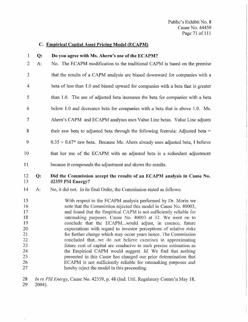
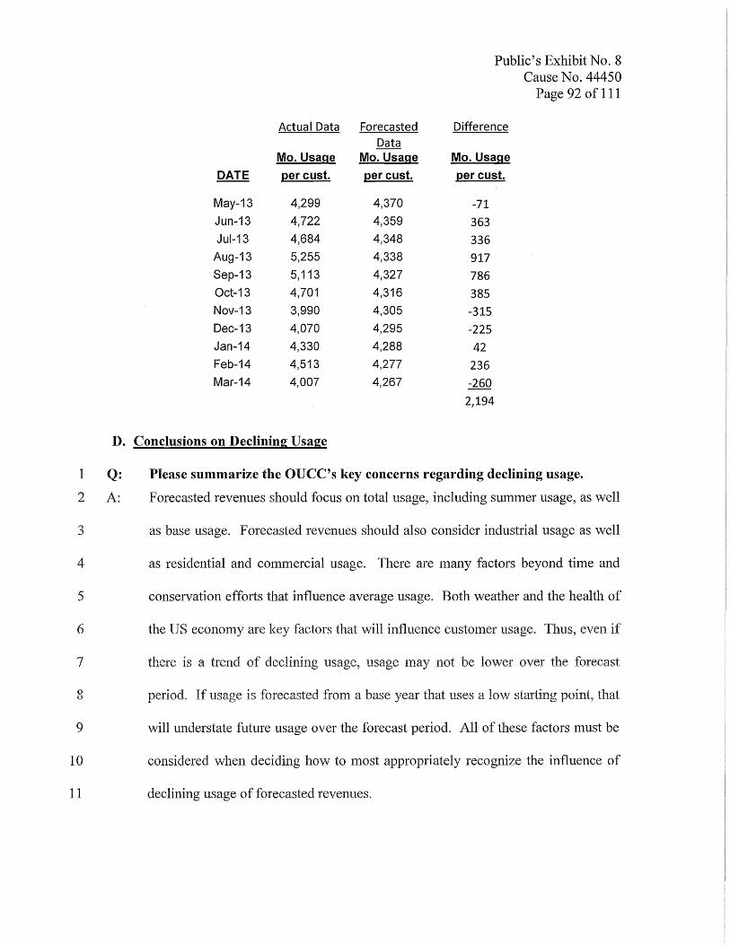
As explained above, Petitioner applied its regression analysis and used

forecasted consumption starting in May 2013. However, in response to auec

discovery (Attachment ERI(-24), Petitioner has provided actual consumption data

for May 2013 through March 2014. By comparing actual to forecasted

consumption, it is clear that Petitioner's forecasted consulnption understated

actual consumption.

1

2

3

4

5

6

7

0 0

9

10

11

Public's Exhibit No.8 Cause No. 44450

Page 92 of 111

Actual Data Forecasted Difference Data

Mo. Usage Mo. Usage Mo. Usage

DATE percust. percust. per cust.

May-13 4,299 4,370 -71

Jun-13 4,722 4,359 363 Jul-13 4,684 4,348 336

Aug-13 5,255 4,338 917

Sep-13 5,113 4,327 786

Oct-13 4,701 4,316 385 Nov-13 3,990 4,305 -315

Dec-13 4,070 4,295 -225

Jan-14 4,330 4,288 42 Feb-14 4,513 4,277 236

Mar-14 4,007 4,267 -260

2,194

D. Conclusions on Declining Usage

Q:

A:

Please summarize the OUCC's key concerns regarding declining usage.

Forecasted revenues should focus on total usage, including summer usage, as well

as base usage. Forecasted revenues should also consider industrial usage as well

as residential and commercial usage. There are many factors beyond time and

conservation efforts that influence average usage. Both weather and the health of

the US economy are key factors that will influence customer usage. Thus, even if

there is a trend of declining usage, usage Inay not be lower over the forecast

period. If usage is forecasted from a base year that uses a lov! starting point, that

will understate future usage over the forecast period. All of these factors must be

considered when deciding how to most appropriately recognize the influence of

declining usage of forecasted revenues.

1 Q: 2

3 A:

4

5

6

7

8

9

10

Public's Exhibit No.8 Cause No. 44450

Page 93 of 111

Please summarize the OUCC's concerns as they specifically relate to Petitioner's analysis.

The regression analysis provided by Petitioner contains autocorrelation and

overstates its predictive power. American Water aclmowledges that 2013 was a

cooler/wetter year and that its usage and revenues were lower due to the weather.

Thus, using a 2013 base year may be a low starting point. Petitioner's winter

weather calculation excludes November and December data. Petitioner's trend

analysis does not use the most current information and excludes late 2013 and

early 2014 data. Finally, Petitioner's trend analysis significantly understates

actual usage for 2013 and 2014.

E. Declining usage and cost of equity

11 Q: 12 13

14 A:

15

16

17

18

19

20

21

22

23

24

While the OUCC has proposed a declining usage adjustment, is there another way to recognize declining consumption other than a direct adjustment to forecasted revenues?

Yes. The influence of declining residential/commercial base consumption could

be considered a risk factor and accounted for through the estimated cost of equity

instead of through an elaborate forecast of future revenues. The influence of

declining residential/commercial base consumption is one of the business risks

faced by many \vater utilities. To the extent the Commission believes declining

residential/commercial base consumption is a risk, that risk could be recognized

through the authorized cost of equity instead of a direct adjustment.

However, if the Commission elects to recognize the risk of declining

usage through its authorized cost of equity, I do not believe it is appropriate to

quantify a specific adjustment to the authorized cost of equity. Instead the

Commission should recognize this risk factor within the range of of estimated

1

2

3

4

5

6

7

8

9

10

11

12 13 14 15 16 17 18 19 20 21

22 Q:

23 A:

24

25

26 Q: 27 A:

Public's Exhibit No.8 Cause No. 44450

Page 94 of 111

costs of equity. Moreover, to the extent that declining residential/commercial

base usage is a risk factor, the companies included in my (and Ms. Ahem's) water

company proxy group also share that risk, and analyses such as the DCF model or

CAPM should reflect most of that risk. Additionally, to the extent the

Commission considers the risk of declining residential/commercial base usage;

the Commission should also consider the benefits that may arise from increasing

summer usage or increasing industrial usage.

This methodology is similar to findings made by the Maine Public Service

Commission in Maine Water Company-Camden & Rockland Division (Order

dated March 25,2014) Docket No. 2013-00362. On page 12 of its Final Order the

Maine Commission found as follows:

Finally, the Company has also seen declining consumption in the residential class over recent years, at a time when it, as well as other water utilities, are facing significant infrastructure replacement needs. As we noted in Docket 2000-175 , "We have not attelnpted to assign a particular value in basis points to any of the factors noted above, and would caution the parties against trying to do so in future rate cases." Docket No. 2000-175, Sept. 29, 2000 Order at 29. As then, we simply state here that the risk factors contribute to our decision to allow a 9.35% return on equity (before floatation costs) that rests in the upper quartile of the range suggested by the analysis.

XVIII. RECOMMENDATIONS

Please..., ...,.,uuunlJ'-".,." your recommendations.

I recommend a cost of equity for Petitioner of 8.6%. I recommend that Pro Forma

present rates be reduced by $1,263,200 to account for residential declining usage

and by $692,000 to account for commercial declining usage.

Does this conclude your testimony?

Yes.

XIX. APPENDIX A

List of Schedules and Attachments

Public's Exhibit No.8 Cause No. 44450

Page 95 of 111

1 Schedule ERI(-l summarizes the results of my cost of equity models.

2 Schedule ERI(-2 contains my DCF analysis.

3 Schedule ERK-3 contains my CAPM analysis. 4 5 Schedule ERI(-4 contains an illustration on how forecasted interest rates influence 6 bond prices.

7 Schedule ERK-5 is flow chart that illustrates Ms. Aheln's models and their results

8 Schedule ERK -6 contains three graphs that compare Ms. Ahem's estimated risk 9 premiums from her PRPM™ analysis vs. the historical risk premium over the

10 same time periods.

11 Schedule ERK-7 illustrates the results of Ms. Ahern's cost of equity models if the 12 PRPM™s are excluded from her analyses.

13 Schedule ERK-8 compares Earned Returns vs. Authorized Returns across water, 14 gas, combination gas & electric, and electric industries.

15 Schedule ERK -9 provides Residential Customer and Consumption Data for 16 January 2004 through December 2013.

17 Schedule ERK-1 0 is regression analyses on residential customer consumption.

18 Attachment ERI(= 1 is a copy of the First Quarter Survey of Professional 19 Forecasters, Federal Reserve Bank of Philadelphia Release (February 14, 2014).

20 Attachment ERK-2 provides the Congressional Budget Office ("CBOs") February 21 2014 The Budget and Economic Outlook: Fiscal Years 2014 to 2024.

22 Attachment ERK-3 shows Selected Yields on bonds as reported by Value Line -23 Selection & Opinion (March 14, 2013).

24 Attachment ERK-4 is an article titled 9% Forever? by Justin Fox published by 25 CNNMoney.com on December 26, 2005.

26 Attachment ERK-5 is a copy of Table C-7 from Morningstar's SBBI 2013 27 Yearbook, Classic Edition. Table C-7 contains historical inflation rates.

Public's Exhibit No.8 Cause No. 44450

Page 96 of 111

1 Attachment ERK-6 is the cover page and page 2 from the March 14, 2014, Value 2 Line Investment Survey - Ratings & Reports.

3 Attachment ERK-7 is page 49 from Duke CFO Magazine Global Business 4 Outlook Survey U.S - First Quarter 2014.

5 Attachment ERK -8 is an article from Schwab Center for Financial Research 6 titled: Q&A: Estimating Long-Term Market Returns (April 11, 2013).

7 Attachment ERI(-9 is an article titled: 30-Year Market Forecast For Investment 8 Planning (2014 edition). This article was published by Forbes. The data was 9 provided by Portfolio Solutions, LLC.

10 Attachment ERI( -lOis a copy of an article by lP. Morgan Asset Management 11 titled: Long-term Capital Market Return Assumptions. (2014 Edition).

12 Attachment ERK-11 is a copy of an article by ING Investment Management titled 13 Long-Term Capital Market Forecasts (February, 192013).

14 Attachment ERK-12 is a copy of an Article by Edward Jones titled: Expectations 15 for Capital Market Returns

16 Attachment ERK-13 is Petitioner's response to OUCC data request (with 17 attachment) 02-010.

18 Attachment ERK-14 contains the cover page and page 37 from Ibbotson's SBBI 19 20 13 Valuation Yearbook.

20 Attachment ERI(-15 contains Petitioner's responses to various OUCC discovery 21 related to dividend policy, capital expenditures and future debt issuances.

22 Attachment ERI( -16 contains the cover page and page 4 from American Water 23 Works ~v1arch 20 14 Institutiona11~vestor Presentation

24 Attachment ERl(-17 contains Petitioner's responses to various OUCC discovery 25 elated to Petitioner's pRPMTM.

26 Attachment ERK-18 contains Petitioner's response and attachment to OUCC 27 discovery request question 7-016

28 Attachment ERI( -19 is an article from California Broker titled How to Get Sued 29 and Lose All Your Clients Using VUL (October 2005).

30 Attachment ERK-20 contains two articles: Roger Ibbotson's Building the Future 31 From the Past and John Campbell's Stock Returns for New Century.

Public's Exhibit No.8 Cause No. 44450

Page 97 of 111

1 Attachment ERK-21 contains pages from Value Line's Selection & Opinion on 2 forecasted, current and historical interest rates from 1999 - 2013.

3 Attachment ERK-22 contains Petitioner's response to OUCC discovery request 4 question 76-008.

5 Attachment ERIZ-23 contains Petitioner's response to OUCC discovery request 6 question 77-001 and 22-010 [Supplemental]

7 Attachment ERK-24 contains Petitioner's response to OUCC discovery request 8 question 66-001 and 79-002 [Supplemental].

9 Attachment ERK -25 explains the Durbin-Watson Statistic by retired Professor 10 Arthur Jensen, California State University, Sacramento.

11 Attachment ERIZ-26 is a copy of a press release issued by American Water Works 12 on April 29, 2014, titled: "American Water Increases Quarterly Dividend by 11 13 Percent. "

xx. APPENDIX B

1 Potential Bias in Analyst Forecasts

Public's Exhibit No.8 Cause No. 44450

Page 98 of 111

2 An article published in the National Regulatory Research Institute (NRRI) Journal

3 of Applied Regulation supports both of my concerns about using unreasonably

4 high growth rates in a DCF analysis with the following: 15

5 Financial research has made it clear that no company, especially a 6 utility, can sustain a growth rate over the long run that exceeds the 7 growth rate of the economy. 15 Since 1959 the long-term sustainable 8 real growth rate in the economy has been about 3.5%.16 If long-term 9 inflation is expected to be about 2.5%, the maximum long-term

10 sustainable nominal growth for any company today is about 6.0%. 11 Since utilities are amongst the slowest growing firms in the 12 economy, a utility today would be expected to have a long-term 13 sustainable growth rate that is significantly below 6%.

14 The article also noted a tendency toward upside bias in analyst forecasts:

15 The other problem with using analyst forecasts as the long-term 16 growth rate in the DCF model is such forecasts are biased to the 17 upside. The evidence on this issue is overwhelming. 17 The forecast 18 bias persists year after year in large part due to the incentive 19 structures in place at many Wall Street firms that tend to reward 20 more optimistic proj ections and to discourage the incorporation of 21 potentially negative views in analysts' forecasts. 18

22 Emphasis added, (Citations included at the end of my testimony).

23 The Wall Street Journal published an article on January 27, 2003 titled

24 Analysts: Still Coming up Rosy. The atiicle discusses how despite a $1.5 billion

25 settlement pending with regulators over stock research-conflicts, analysts are

26 unshaken in their optimism that most of the companies they cover will have above

15. How improper risk assessment leads to overstated required returns for utility stocks by Steven G. Kihrn NRRI Journal of Applied regulation-Volume 1, June 2003, p. 98.

1

2

3 4 5 6 7

8 9

10 11 12

13

14

15

16

17 18 19 20

21 22 23

24

25

26 27 28 29 30 31 32 33

Public's Exhibit No.8 Cause No. 44450

Page 99 of 111

average double-digit growth rates during the next several years. The article

asserts that such growth is unlikely:

And:

Historically, growth in corporate earnings has slightly lagged nominal growth in gross domestic product. In other words, profits can only grow as fast as the economy. Right now, optimistic Wall Street analysts expect earnings to defy history and grow far faster than that.

Those overly optimistic growth estimates also show that, even with all regulatory forces on too-bullish analysts allegedly influenced by their firms' investment-banking relationships, a lot of things haven't changed: Research remains rosy and many believe it always will.

The concern regarding bias in intermediate term analyst forecasts (such as

those relied upon by Ms. Ahern) is also mentioned in The real cost of equity by

Marc H. -Goedhart, Timothy M. Koller and Zane D. Williams (McKinsey

Quarterly Autumn 2002):

Some theorists have attempted to meet this challenge by surveying equity analysts, but since we Imow that analyst projections almost always overstate the long-term growth of earnings or dividends,2 analyst objectivity is hardly beyond question.

(Citations included at the end of my testimony).

In a more recent article; Equity analysts: Still too bullish by Marc H.

Goedhart, Rishi Raj and Abhishek Saxena (McKinsey Quarterly - April 2010) the

authors reiterated the concern regarding analyst forecast bias:

No executive would dispute that analysts' forecasts serve as an important benchmark of the current and future health of companies. To better understand their accuracy, we undertook research nearly a decade ago that produced sobering results. Analysts, we found, were typical overoptimistic, slow to revise their forecasts to reflect new economic conditions, and prone to making increasingly inaccurate forecasts when economic growth declined. 1

Public's Exhibit No.8 Cause No. 44450 Page 100 of 111

1 Alas, a recently completed update of our work only reinforces this 2 view - despite a series of rules and regulations, dating to the last 3 decade, that were intended to improve the quality of the analysts' 4 long -term earnings forecasts, restore investor confidence in them, 5 and prevent conflicts of interest. 2 F or executives, many of whom 6 go to great lengths to satisfy Wall Street's expectations in their 7 financial reporting and long-term strategic moves, this is a 8 cautionary tale worth remembering.

9 (Citations included at the end of my testimony).

10 Also, the Abstract of an Article titled, Do Analyst Conflicts Matter? Evidence

11 from Stock Recommendations by Anup Agrawal and Mark Chen (Journal of Law

12 and Economics, 2008, V 51), includes the following statement:

13 However, evidence from the response of stock prices and trading 14 volumes to upgrades and downgrades suggests that the market 15 recognizes analyst conflicts and properly discounts analyst options. 16 17 While it predates the October 31, 2003, final judgment in the Global Research

18 Analyst Settlement ("GRAS"), the following article: Stock Analysts Still Put

19 Their Clients First, Financial Analysts Journal, Volume 59 Issue 3, May 1, 2003,

20 discusses the separation of research and investment banking services and its

21

22

23

24 25 26 27 28 29 30 31 32 33

influence on analyst estilnates. The article concludes that the separation of

research and investment banking services has not resolved the concern that

analyst forecasts are still upwardly biased. Page 5 of the article states as follows:

The new requirements imply that independent research (brokerage research without investment banking ties) is better for investors. But why independent analysts will be less vulnerable than brokerage film analysts to the same pressures for optimism is unclear. Analysts themselves have retnarked that one source of strong pressure for "optimism biases" in recommendations is the need to keep access to the managers of the companies they cover; in other words, issue positive research or expect to be cut off from management guidance. Unfortunately, the Sarbanes-Oxley bill, which mandated many improvements in corporate managers'

Public's Exhibit No.8 Cause No. 44450 Page 101 of 111

1 financial practices, did nothing to reduce the unethical practice by 2 many managers of communicating only with those analysts who 3 "cooperate" with management's implicit (and usually positive) 4 forecasts of the future. 6 Finding a way to fix this blind spot may be 5 more important than all the other "sticks" regulating analysts 6 combined.

7 Interestingly, the Wall Street Journal reported in April 2003 that 8 after reviewing disclosure reports issued as a result of the new 9 requirements, they concluded that the brokerage firms of the top

10 investment bank:s are still more likely to give optimistic research 11 recommendations to their own banking clients. Of course, the new 12 disclosure requirements attempt to protect investor clients by 13 making them aware of investment research's potential as an 14 advertising medium, but the attempt works only if investors read 15 and understand the disclosures. Institutional investors are probably 16 more likely than retail investors to read, put into context, and fully 17 appreciate these new disclosures.

18 Emphases added

19 (See Table of Citations at end of my testimony).

20 While the GRAS may have reduced some of the causes of analyst bias, I

21 do not believe the problem of optimistic analyst forecasts has been eliminated.

22 Moreover, the Equity analysts: Still too bullish atiicle by Goedhart, Raj and

23 Saxena and Do Analyst Conflicts Matter? Evidence from Stock

24 Recommendations by Agrawal and Chen were both published several years after

25 the GRAS. Both article support the opinion that concerns about analyst optimism

26 still exist.

27 When using analyst forecasts of EPS to estirnate growth (g) in a DCF

28 analysis, both the potential for analyst bias and the intermediate term nature of the

29 forecasts may make these estimates unreliable. Even assuming no analyst bias,

30 unsustainable growth rates should be adjusted or given reduced weight.

1

2

3

4

5

6 7 8 9

10 11

12 13 14 15 16

17 18 19 20 21 22 23 24 25 t"\r L,O

27 28 29

XXI. APPENDIX C

Public's Exhibit No.8 Cause No. 44450 Page 102 of 111

Sources Supporting the Use of the Geometric Mean

In VALUATION Measuring and Managing the Value of Companies (Second

Edition) by Tom Copeland, Tim K.oller and Jack Murrin on pages 260 - 261 the

text specifically advocates the use of the geometric mean over the arithmetic

mean to estimate cost of equity in a CAPM analysis:

We recommend using a 5 to 6 percent market risk premium for U.S. companies. This is based on the long-run geometric average risk premium for the return on the S&P 500 versus the return in long term government bonds from 1926-1992.4 Since this is a contentious area that can have a significant impact on valuations, we elaborate our reasoning in detail here.

We use a very long time frame to measure the premium rather than a short time frame to eliminate the effects of short-term anomalies in the measurement. The 1926-1992 time frame reflects wars, depressions and booms. Shorter time periods do not reflect as diverse a set of economic circumstances.

We use a geometric average of rates of return because arithmetic averages are biased by the measurement period. An arithmetic average estimates the rates of return by taking a simple average of the single period rates of return. Suppose you buy a share of nondividend-paying stock for $50.00. After one year the stock is worth $100. After two years the stock falls to $50 once again. The first period return is 100 percent; the second period return is -50 percent. The arithrlletic average return is 25 percent [(100 percent - 50 percent) / 2]. The geometric average is zero. (The geometric average is the compound rate of return that equates the beginning and ending value.) (sic) We believe the geometric average represents a better estimate of investors' expected return over long periods of time.

1 2 3

4 5

6

7

8 9

10 11 12 13 14 15 16 17 18 19

20

21

22

23

24

25

Public's Exhibit No.8 Cause No. 44450 Page 103 of 111

Finally, we calculate the premium over long-term government bond returns to be consistent with the risk free rate we use to calculate the cost of equity.

(See Table of Citations at end of my testimony). Italics emphasis in original, underlined emphases added.

return:

At page 263, the text notes other weaknesses of relying on an arithmetic

Note that the arithmetic return is always higher than the geometric return and that the difference between them becomes greater as a function of the variance of returns. Also the arithmetic average depends upon the interval chosen. For example, an average of monthly returns will be higher than an average of annual returns. The geometric average, being a single estimate for the entire time interval, is invariant to the choice of interval. Finally, empirical research by Fama-French (1988), Lo and MacI(inlay (1988), and Poterba and Summers (1988) indicates that a significant long-term negative autocorrelation exists in stock returns.5 Hence, historical observations are not independent draws from a stationary distribution.

(See Table of Citations at end of my testimony)

On pages 259-260 of the text, the authors recommend using the 10-year Treasury

bond rate. 16

The text Analysis of Equity Investments: Valuatlon also supports the use

of the geometric mean to estimate the market risk premium. On page 50, the

authors state that geometric means produce estilnates of the equity risk premium

that are more consistent with economic theory:

16. Note, in the chart displayed on page 261, the text shows risk premiums based on the arithmetic average and the geometric average. Although not explicitly stated in the text, both calculations are based on total bond returns and not income returns. This is relevant because Ms. Ahern argues that one should use income returns vs. total returns to estimate the risk premium.

Public's Exhibit No.8 Cause No. 44450 Page 104 of 111

1 Although the debate is inconclusive, this book uses the geometric 2 means, not only for the previously given reasons but also because 3 geometric means produce estimates of the equity risk premium that 4 are more consistent with the predictions of economic theory.14

5 (See Table of Citations at end of my testimony)

6 Analysis of Equity Investments: Valuation is written by the Association for

7 Investment Management and Research and is produced as a study guide for the

8 Chartered Financial Analyst (CF A) program.

9 In an article titled Equity Risk Premiums (ERP): Determinants,

10 Estimations and Implications - The 2013 Edition (p. 26) by Dr. Aswath

11 Damodaran, Dr. Damodaran supports the use of a geometric mean risk premium:

12 The final sticking point when it comes to estimating historical 13 premiums relates to how the average returns on stocks, treasury 14 bonds and bills are computed. The arithmetic average return 15 measures the simple mean of the series of annual returns, whereas 16 the geometric average looks at the compounded returnS1 . Many 1 7 estimation services and academics argue for the arithmetic average 18 as the best estimate of the equity risk premium. In fact, if annual 19 returns are uncorrelated over time, and our objective was to 20 estimate the risk premium for the next year, the arithmetic average 21 is the best and most unbiased estimate of the premium. There are, 22 however, strong arguments that can be made for the use of 23 geometric averages. First, ernpirical studies seenl to indicate that 24 returns on stocks are negatively correlatedS2 over time. 25 Consequently, the arithmetic average return is likely to over state 26 the premium.

27 Emphases added

28 (See Table of Citations at end of my testimony)

XXII. APPENDIX D

Forecasted Market Risk Premiums

Public's Exhibit No.8 Cause No. 44450 Page 105 of 111

1 Building the Future from the Past by Roger Ibbotson (June 2002) forecasts an 2 equity risk premium of less than 4.0% (Attachment ERIC 20).

3 Stock returns for a New Century by John Campbell (Professor of Applied 4 Economics, Harvard University) (June 2002) forecasts an equity risk premium of 5 1.5% to 2.0% (Attachment ERIC 20).

6 The Real Cost of Equity by Marc H. Goedhart, Timothy M. Koller and Zane D. 7 Williams of McKinsey Quarterly (October 2002) asserts as follows "The 8 inflation-adjusted cost of equity has been remarkably stable for 40 years, implying 9 a current equity risk premium of 3.5 to 4 percent."

10 Corporate Finance: New evidence puts risk premium in context by Elroy Dimson, 11 Paul Marsh, and Mike Stauton (London Business School) (March 2003) forecasts 12 a geometric equity risk premium of 2.50/0 to 4.0% and an arithmetic mean risk 13 premium of around 3.5% to 5.25%. The article notes that these estimates are 14 lower than historical premia quoted in most text books and surveys of market 15 professionals.

16 Thoughts on Social Security Reform by Goldman Sachs (January 18, 2005) 17 discusses the assumptions used by the US Government to discuss Social Security 18 reform. Page 22 of the atiicle states as follows: "The Commission assumed that 19 personal accounts would earn real returns of 6.5% on equities, 3.5% on corporate 20 bonds and 3% on Treasury Bonds." This implies a risk premium of 3.5%. Note 21 the Goldman Sachs atiicle asserts that the "Return Assumptions are Too High".

22 Survey of Profession Forecasted by Federal Reserve Bank of Philadelphia 23 (February 14, 2014) estimates the return on stocks, over the next ten years to be 24 6.0% and the return on 10 year US Treasury bonds to be 4.35%. T'hese estimates 25 imply a risk premium 1.65%. (Attachment ERIC 1)

26 Q&A: Estimating Long-Term Market RetulTIS: by the Schwab Center for 27 Financial Research, (April 2013). Page 4 of the report estimates Long-term risk 28 premiums of 3.6% for Large stocks and 5.1 % for Mid/Slnall stocks. (Attach111ent 29 ERIC 8)

30 Dr. Aswath Damodaran, a Professor at the Stern School of Business at New York 31 University maintains a web page (http://pages.stern.nyu.edul~-'adamodarD. Each 32 month he calculates an "Implied Equity Risk Premium" and presents his findings 33 on his web page. Dr. Damodaran's estimated risk premium as of March 1, 2014 34 was 4.96%.

XXIII. APPENDIX E

Public's Exhibit No.8 Cause No. 44450 Page 106 of 111

1 Support for a single digit cost of equity

2 An article by California Broker titled How to Get Sued and Lose Your Clients

3 Using VUL asserts "Illustrating 10% to 12% Equity returns is Dangerous and

4 Wrong." (Attachment ERK 19). The article further states as follows:

5 The SEC allows carriers to illustrate hypothetical future returns. 6 Variable life illustrations must show a 0% return, a 6% return and 7 a rate "not greater than 12%". Many carriers think it is acceptable 8 to illustrate equity sub-accounts at 10% to 12% simply because the 9 SEC allows them to do so. Many agents using data from a highly

10 unusual period, still believe that domestic equities are expected to 11 grow at better than 10% per year. These agents believe that it is 12 prudent to illustrate 10% returns and base premium payments upon 13 equity sub-accounts growing at this rate of return. I disagree and I 14 believe that illustrating these returns is irresponsible and invites 15 legal liability for the following reasons:

16 Emphasis added

17 An article entitled Son, Don't Count On Double-Digit Stock Returns

18 appeared in the June 26, 2000 edition of Business Week web page, refers to a

19 study performed by Eugene Fama and K.enneth French. According to the article:

20 Fama and French argue that over the long nln, stocks are likely to 21 outperform risk free debt by only 3% to 3.5% a year.

22 Fama and French estimate that in the future, stocks will return to 23 more like their pre 1950 norm. Says French: "We're saying that if 24 you're a pension fund, you ought to pencil in returns of 3% to 25 3.5% [above the risk free rate] for the next 30 years."

26 However, if you're a 30-year old who's not saving much because 27 you're relying on making returns just as profitable as those in the 28 past decades from now until you retire, think again-or you just 29 might end up living on dog food and government cheese.

30 Emphasis added

Public's Exhibit No.8 Cause No. 44450 Page 107 of 111

1 While this article is somewhat dated, a risk premium of 3.0% to 3.5% is

2 consistent with many of the articles cited earlier in my testimony. The current

3 long-term risk free rate was 3.92% as of the close of business on December 6,

4 2013. If the long-term risk free rate is combined with the Fama - French risk

5 premium of3.0% to 3.5%, it results in an expected return of7.02% to 7.56%

6 In his book Stocks for the Long Run, Jeremy J. Siegel discusses the long-

7 term stability of real returns for equities. On page 11 he states as follows:

8 It is clear that the growth of purchasing power in equities not only 9 dominates all other assets but is remarkable for its long-term

10 stability. Despite extraordinary changes in the economic, social 11 and political environment over the past two centuries, stocks have 12 yielded between 6.6 percent and 7.2 percent per year after inflation 13 in all major subperiods.

14 Dr. Siegel further states on page 12 as follows:

15 Note the extraordinary stability of the real returns on stocks over 16 all major subperiods: 7.0 percent from 1802-1870, 6.6% from 17 1871-1925 and 7.2% from 1926-1997.

18 If forecasted inflation ranges from 2.3% to 2.5% and real returns range from 6.6%

19 to 7.2% it produces a range of expected equity returns of 9.66% to 9.88%

20 (1.023[2.3% inflation] * 1.072 [7.2% real return] = 1.0966, translates into a

21 9.66% return).

22 Additional articles suppoli a total market return below 10.0%. For

23 example, an article written by Justin Fox in CNNMoney.com (December 26,

24 2005) 9% Forever?, the author notes that Roger Ibbotson's long run forecast for

25 stock returns is 9.27%. The article also notes that Rob Arnott, Pasadena money

26 manager and editor of the Financial Analysts Journal disagrees with Dr. Ibbotson

27 and thinks future equity returns could be below 6%. (Attachment ERI( 4)

XXIV. APPENDIX F

1 General Problems with Analyst Forecasts

Public's Exhibit No.8 Cause No. 44450 Page 108 of 111

2 On page 106 of her book The Equity Risk Premium - The Long Run future of the

3 Stock Market, Bradford Cornell states as follows:

4 The practical problem raised by relying on analysts' forecasts is 5 that such forecasts typically have short horizons. Services that 6 aggregate such forecasts, including those by IBES and Zack's 7 Investment Research, do not provide forecasts beyond 5 years. 8 From the standpoint of the DCF model, which extends into 9 perpetuity, this horizon is too short.

10 Emphasis added

11 Mr. Cornell goes on to discuss the problems with assuming that the forecasted

12 growth rate can be maintained in perpetuity.

13 In most cases, the IBES forecasts are greater than the long-run 14 economic growth rates. Such growth rates clearly cannot be 15 maintained forever. Although it is possible that a company's 16 dividends can grow significantly faster than the general economy 17 for 5 years, if such a growth rate were maintained indefinitely, the 18 company would eventually engulf the entire economy.

19 Also the Cost of Capital - Estimation and Application 2nd edition by

20 Shannon Pratt makes the following assertions about using analyst forecasts to

21 estimate cost of equity:

22 It is theoretically impossible for the sustainable perpetual growth 23 rate for a company to significantly exceed the growth rate in the 24 economy. Anything over a 6-7% perpetual growth rate should be 25 questioned carefully.

26 A COlTIn10n approach to deriving a perpetual growth rate is to 27 obtain stock analysts' estimates of earnings growth rates. The 28 advantage of using these growth estimates is that they are prepared 29 by people who follow these companies on an ongoing basis. These 30 professional stock analysts develop a great deal more insight on

1 2

3

4 5 6 7

8 9

10 11 12

13 14 15 16 17 18 19 20 21 22 23

24 25 26

Public's Exhibit No.8 Cause No. 44450 Page 109 of 111

these companies than a causal investor or valuation analyst not specializing in the industry is likely to achieve.

There are however, three caveats when using this information:

1. These earnings growth estimates typically are for only the next two to five years; they are not perpetual. Therefore, any use of these forecasts in a single-stage DCF model must be tempered with a longer-term forecast.

2. Most published analysts' estimates come from "sell-side" stock analysts who work for firms that are in the business to sell stocks. Thus, although their earnings forecasts fall within the range of "reasonable" possibilities, they may be on the high end of the range.

3. Usually these estimates are obtained from firms that provide consensus earnings forecasts; that is, they aggregate forecasts from a number of analysts and report certain summary statistics (mean, median, etc.) on these forecasts. For a small publically traded firm, there may be only one or even no analyst following the company. The potential for forecasting errors is greater when the forecasts are 0 btained from a very small number of analysts. These services typically report the number of analysts who have provided earnings estimates, which should be considered in determining how much reliance to place on forecasts of this type.

Many of the problems inherent in using a single-stage model to estimate cost of capital are addressed by using a multistage model.

1 2 3

4 5

6 7 8

9 10 11

12 13

14 15

16 17 18 19 20 21 22 23 24

25 26

27 28

Page 98

Page 99

Page 100

Page 101

Page 102

xxv. TABLE OF CITATIONS

Public's Exhibit No.8 Cause No. 44450 Page 110 of 111

Footnote 15: Robert D. Arnott and Peter L. Bernstein "What Risk Premium is Normal? Financial Analysts Journal, 58 (2) March/April 2002): 64-85.

Footnote 16: Source Council of Economic Advisors, Economic Report of the President, 2002.

Footnote 1 7: See for example, Vij ay Kumar Chopra, "Why So Much Error in analysts' Earnings Forecasts?" Financial Analysts Journal, 54(6) November/December 1998): 35-42.

Footnote 18: See Masakao N. Darrough and Thomas Russal, "A Positive Model of Earnings Forecasts: Top Down Versus Bottom Up." Journal of Business, 75(1) (January 2002) 127-52.

Footnote 2: See Marc H. Goedhart, Brendan Russel and Zane Williams, "Prophets and profits?" McKinsey on Finance, Number 2, Autumn 2001.

Footnote 1: See Marc H. Goedhart, Brendan Russel and Zane Williams, "Prophets and profits?" McKinsey on Finance, Number 2, Autumn 2001.

Footnote 2: US Securities and Exchange Commission (SEC) Regulation Fair Disclosure (FD), passed in 2000, prohibits the selective disclosure of material information to some people but not others. The Sarbanes-Oxley Act of 2002 includes provisions specifically intended to help restore investor confidence in the reporting of securities' analysts, including a code of conduct for them and a requirement to disclose knowable conflicts of interest. The Global Settlement of 2003 between regulators and ten of the largest US Investment firms aimed to prevent conflicts of interest between their analyst and investment businesses.

Footnote 6: The Sarbanes-Oxley bill may be found at banking. senate. gov/pss/acctrfm/conf_fpt.pdf.

Footnote 4 of the text cites to Ibbotson Associates, Stocks, Bonds, Bills and Inflation 1993 Yearbook (Chicago, 1993).

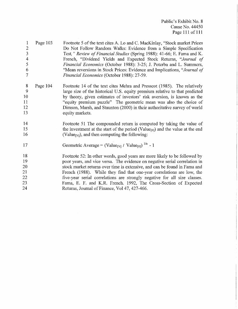
1 2 3 4 5 6 7

8 9

10 11 12 13

14 15 16

17

18 19 20 21 22 23 24

Page 103

Page 104

Public's Exhibit No.8 Cause No. 44450 Page 111 of 111

Footnote 5 of the text cites A. Lo and C. MacKinlay, "Stock market Prices Do Not Follow Random Walks: Evidence from a Simple Specification Test, " Review of Financial Studies (Spring 1988): 41-66; E. Fama and K. French, "Dividend Yields and Expected Stock Returns, "Journal of Financial Economics (October 1988): 3-25; J. Poterba and L. Summers, "Mean reversions in Stock Prices: Evidence and Implications, "Journal of Financial Economics (October 1988): 27-59.

Footnote 14 of the text cites Mehra and Presscot (1985). The relatively large size of the historical U.S. equity premium relative to that predicted by theory, given estimates of investors' risk aversion, is known as the "equity premium puzzle" The geometric mean was also the choice of Dimson, Marsh, and Staunton (2000) in their authoritative survey of world equity markets.

Footnote 51 The compounded return is computed by taking the value of the investment at the start of the period (Value[o]) and the value at the end (Value[N]), and then computing the following:

Geometric Average = (Value[N] / Value[o]) lin - 1

Footnote 52: In other words, good years are more likely to be followed by poor years, and vice versa. The evidence on negative serial correlation in stock market returns over time is extensive, and can be found in Fama and French (1988). While they find that one-year correlations are low, the five-year serial correlations are strongly negative for all size classes. Fama, E. F. and K.R. French. 1992, The Cross-Section of Expected Returns, Journal of Finance, Vol 47, 427-466.

AFFIRMATION

I affirm, under the penalties for perjury, that the foregoing representations are true.

Cause No. 44450 Indiana-American Water Co., Inc.

Edward R. Kaufman Indiana Office of Utility Consumer Counselor

May 2,2014 Date

Cause No. 44450 Schedule ERK 1 Page 1 of 2

SUMMARY OF COST OF EQUITY STUDIES

DCF Studies:

Value Line Proxy Group

DCF Study using 3 month: Dividend yield: (Schedule 2) 8.36%

DCF Study using 6 month: Dividend yield: (Schedule 2) 8.39%

Growth in Forecasted Earnings Per Share (Only)

DCF Study using 3 month: Dividend yield: (Schedule 2)

DCF Study using 6 month: Dividend yield: (schedule 2)

Multi - Stage DCF Model

Range of DCF Studies :

CAPM Studies

Value Line Proxy Group

Historical Risk Premiums

CAPM Study using Long term interest rates: (Schedule 3, page 3)

9.51%

9.54%

8 . 37%

8 . 36% - 9 . 54%

7 . 4 5% - 7 . 47%

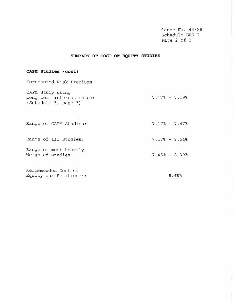
Cause No. 44388 Schedule ERK 1 Page 2 of 2

SUMMARY OF COST OF EQUITY STUDIES

CAPM Studies (cont)

Forecasted Risk Premiums

CAPM Study using Long term interest rates: (Schedule 3, page 3)

Range of CAPM Studies:

Range of all Studies:

Range of most heavily Weighted studies:

Recommended Cost of Equity for Petitioner:

7.17% - 7.19%

7.17% - 7.47%

7.17% - 9.54%

7.45% - 8.39%

8 .. 60%

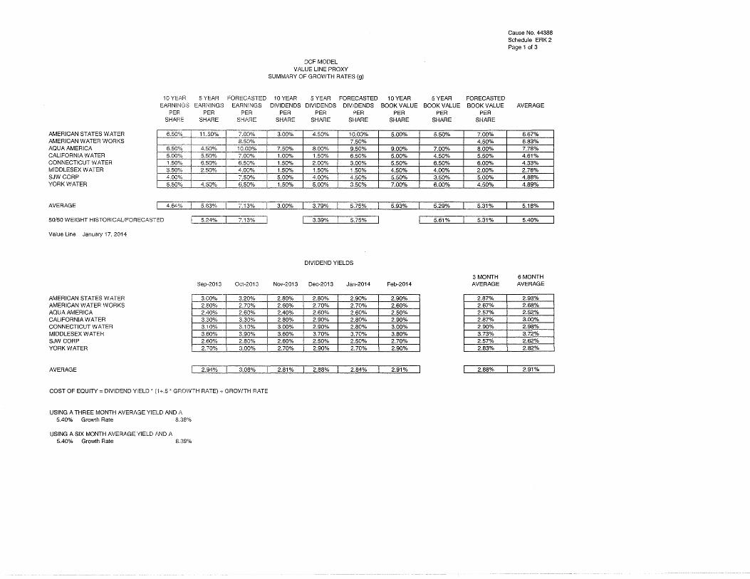
AMERICAN STATES WATER AMERICAN WATER WORKS AQUA AMERICA CALIFORNIA WATER CONNECTICUT WATER MIDDLESEX WATER SJW CORP YORK WATER

10YEAR 5 YEAR EARNINGS EARNINGS

PER PER SHAR:E SHARE

r---::-=-:--

~ --11.50%

1--::-::-:--~- __ 4.50%

~- __ 5.50% __

1.50% 6.50% 3.50% 2.50%

~ '----S __ QQ% __ _~§Ojlo

FORECASTED EARNINGS

PER SHARE

"1.00% 8.50% 10.00% 7.00%

'6.S0% 4.00% 7.50% 6.S0%

--

DCF MODEL VALUE LINE PROXY

SUMMARY OF GROWTH RATES (g)

10 YEAR 5 YE.AR FORECASTED 10 YEAR 5 YEAR FORECASTED DIVIDENDS DIVIDENDS DIVIDENDS BOOK VALUE BOOK VALUE BOOK VALUE

PER SHARE

3.00%

7.50% 1.00% 1.50% 1.50% 5.00% 1.50%

PER SHARE

4.50%

8.00% 1.50% 2.00% 1.50% 4.00% S.OO%

PER SHARE

10.00% 7.50% 9.50% 6.50% 3.00% 1.50% 4.50% 3.50%

PER SHARE

5.00%

9.00% 5.00% 5.50% 4.50% 5.50% 7.00%

PER SHARE

5.50%

7.00% 4.50% 6.50% 4.00% 3.50% 6.00%

PER SHARE

7.00% 4.50% 8.00% 5.50% 6.00% 2.00% 5.00% 4.S0%

Cause No. 44388 Schedule ERK 2 Page 1 of 3

AVERAGE

6.67% 6.83% 7.78% 4.61% 4.33% 2.78% 4.88% 4.8~

AVERAGE I 4.64~~ 5.83% ]7:13%~~-1~ 3.Oo}i;==C).79% 5.75% 5.93% 5.29% 5.31% -C~5.18%

50/50 WEIGHT HISTORICAUFOREG.ASTED

Value Line January 17,2014

AMERICAN STATES WATER AMERICAN WATER WORKS AQUA AMERICA CALIFORNIA WATER CONNECTICUT WATER MIDDLESEX WATEk SJW CORP YORK WATER

C 5.24% ~'.13% I

Sep-2013 Oct-2013

3.00% 3.20% __ 2.80% 2.70%

2.40% ,?60% 3.30% 3.30% 3.'10% 3.10% 3.60% 3.90% 2.60% 2.80% 2.70% 3.00%

3.39% 5~

DIVIDEND YIELDS

Nov-2013 Dec-2013 Jan-2014

2.80% 2.80% 2.90% 2.60% 2.70% 2.70% 2.40% 2.60% 2.60% 2.80% 2.90% 2.80% 3.00% 2.90% 2.80% 3.60% 3.70% 3.70% 2.60% 2.50% 2.50% 2.70% 2.900f0~~_ ~ 2.70% '---_

~%--~~Olo 5.40%

Feb-2014

2.90% 2.60% 2.50% 2.90% 3.00% 3.80% 2.70% g.@O~

3 MONTH AVERAGE

2.87% 2.67% 2.57% 2.87% 2.90% 3.73% 2.57% 2.83%

6 MONTH AVERAGE

2.93% 2.68% 2.52% 3.00% 2.98% 3.72% 2.62% 2.82%

AVERAGE L 2.94%] 3.08%_ 2.81% 2.88% 2.84% 2.91% J ~~-I--~2.91%

COST OF EQUITY = DIVIDEND YIELD * ('1+.5 * GROWTH RATE) + GROWTH RATE

USING A THREE MONTH AVERAGE YIELD AND 5.40% Growth Rate 8.:36%

USING A SIX MONTH AVERAGE YIELD AND A 5.40% Growth Rate 8.:39%

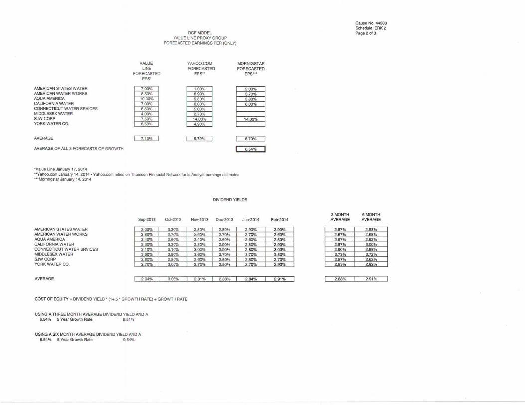
AMERICAN STATES WATER AMERICAN WATER WORKS AQUA AMERICA CALIFORNIA WATER CONNECTICUT WATER SRVICES MIDDLESEX WATER SJW CORP YORK WATER CO.

AVERAGE

AVERAGE OF ALL 3 FORECASTS OF GROWTH

' Value Line January 17, 2014

VALUE LINE

FORECASTED EPS'

7.00% 8.50% 10.00% 7.00% 6.50% 4.00% 7.50%

'---_§J50% _

7.13%

DCF MODEL VALUE LINE PROXY GROUP

FORECASTED EARNINGS PER (ONLY)

YAHOO.COM FORECASTED

EPS"

1.00% 6.90% 5.80% 6.00% 5.00% 2.70% 14.00% 4.90%

5.79%

MORNIGSTAR FORECASTED

EPS'"

2.00% 5.70% 5.80% 6.00%

_.14..&0%

6.70%

6.54%

" Yahoo. com January 14, 2014 - Yahoo.com relies on Thomson Finnacial Network for is Analyst earnings estimates "'Mornngstar January 14, 2014

AMERICAN STATES WATER AMERICAN WATER WORKS AQUA AMERICA CALIFORNIA WATER CONNECTICUT WATER SRVICES MIDDLESEX WATER SJW CORP YORK WATER CO.

Sep-2013

3.00% 2.80% 2.40% 3.30% 3.10% 3.60% 2.60% 2.70%

Oct-201 3

3.20% 2.70% 2.60% 3.30% 3.10% 3.90% 2.80% 3.00%

DIVIDEND YIELDS

Nov-201 3 Dec-2013 Jan-201 4

2.80% 2.80% 2.90% 2.60% 2.70% 2.70% 2.40% 2.60% 2.60% 2.80% 2.90% 2.80% 3.00% 2.90% 2.80% 3.60% 3.70% 3.70% 2.60% 2.50% 2.50% 2.70% 2.90% 2.70%

Feb-2014

2.90% 2.60% 2.50% 2.90% 3.00% 3.80% 2.70% 2.90%

AVERAGE 2.94% 3.08% 2.81% 2.88% 2.84% 2.91%

COST OF EQUITY = DIVIDEND YIELD ' (1+.5 ' GROWTH RATE) + GROWTH RATE

USING A THREE MONTH AVERAGE DIVIDEND YIELD AND A 6.54% 5 Year Growth Rate 9.51%

USING A SIX MONTH AVERAGE DIVIDEND YIELD AND A 6.54% 5 Year Growth Rate 9.54%

3 MONTH AVERAGE

2.87% 2.67% 2.57% 2.87% 2.90% 3.73% 2.57% 2.83%

Cause No. 44388 Schedule ERK 2 Page 2 of3

6 MONTH AVERAGE

2.93% 2.68% 2.52% 3.00% 2.98% 3.72% 2.62% 2.82%

2.88% 2.91 %

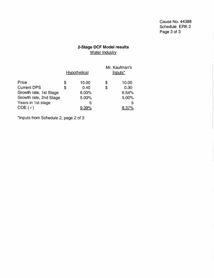
Price $ Current DPS $ Growth rate, 1 st Stage Growth rate, 2nd Stage Years in 1 st stage COE ( r)

2-Stage DCF Model results Water Industry

Hypothetical

10.00 0.40

6.000/0 5.00%

5 9.39%

Mr. Kaufman's Inputs*

$ $

10.00 0.30

6.54% 5.00%

5 8.37%

*Inputs from Schedule 2, page 2 of 3

Cause No. 44388 Schedule ERK 2 Page 3 of 3

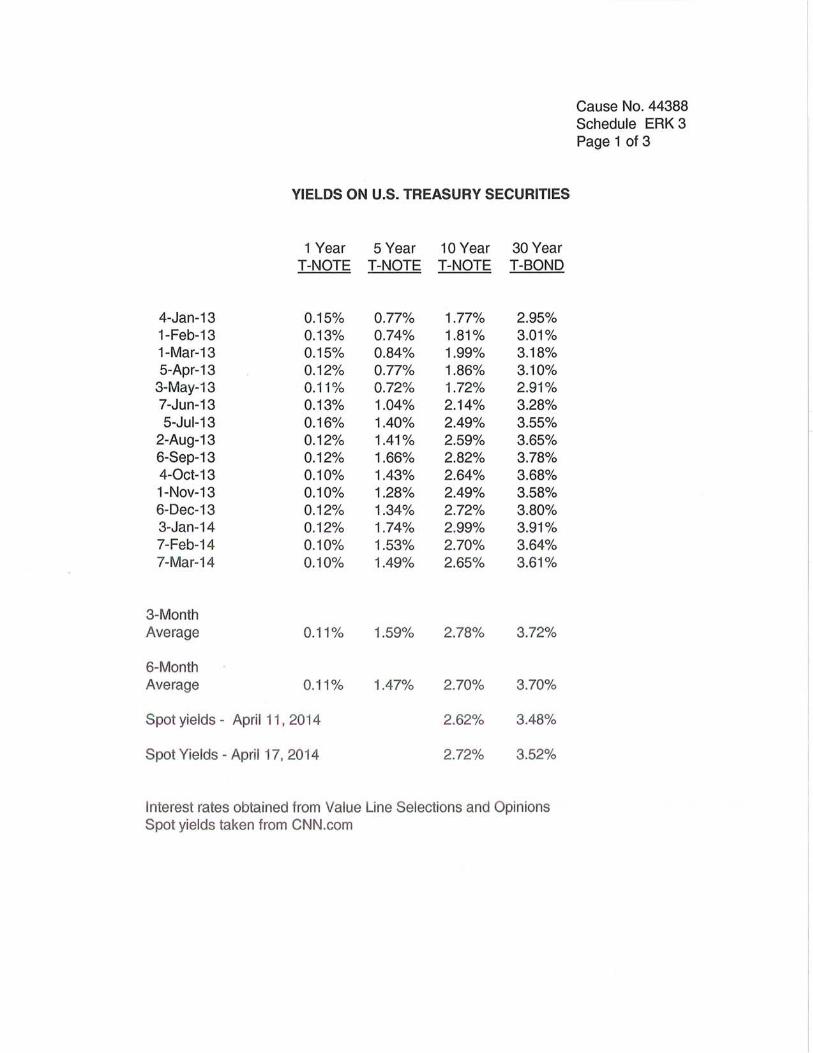
YIELDS ON U.S. TREASURY SECURITIES

1 Year 5 Year 10 Year T -NOTE T -NOTE T -NOTE

4-Jan-13 0.15% 0.770/0 1.77% 1-Feb-13 0.13% 0.74% 1.81 % 1-Mar-13 0.15% 0.84% 1.99% 5-Apr-13 0.12% 0.770/0 1.86%

3-May-13 0.11% 0.720/0 1.720/0 7-Jun-13 0.13% 1.04% 2.14% 5-Jul-13 0.16% 1.40% 2.49%

2-Aug-13 0.12% 1.41% 2.59% 6-Sep-13 0.12% 1.66% 2.82% 4-0ct-13 0.10% 1.43% 2.640/0 1-Nov-13 0.100/0 1.28% 2.49% 6-Dec-13 0.120/0 1.34% 2.72% 3-Jan-14 0.12% 1.74% 2.990/0 7-Feb-14 0.100/0 1.53% 2.70% 7-Mar-14 0.10% 1.49% 2.65%

3-Month Average 0.11 0/0 1.590/0 2.78%

6-Month Average 0.11 % 1.47% 2.70%

Spot yields - April 11, 2014 2.62%

Spot Yields - April 17,2014 2.72%

30 Year T-80ND

2.95% 3.01 % 3.180/0 3.10%

2.91% 3.280/0 3.550/0 3.65% 3.780/0 3.68% 3.58% 3.80% 3.91% 3.64% 3.61 %

3.720/0

3.70%

3.48%

3.52%

Interest rates obtained from Value Line Selections and Opinions Spot yields taken from CNN.com

Cause No. 44388 Schedule ERK 3 Page 1 of 3

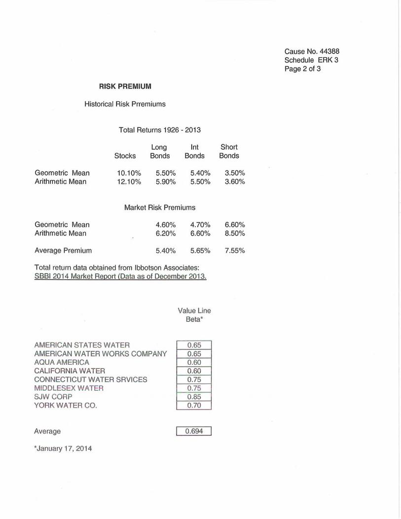
RISK PREMIUM

Historical Risk Prremiums

Total Returns 1926 - 2013

Long Int Stocks Bonds Bonds

Geometric Mean 10.10% 5.50% 5.400/0 Arithmetic Mean 12.100/0 5.90% 5.500/0

Market Risk Premiums

Geometric Mean Arithmetic Mean

Average Premium 5.400/0

Total return data obtained from Ibbotson Associates: SBBI 2014 Market Report (Data as of December 2013.

AMERICAN STATES WATER AMERICAN WATER WORKS COMPANY AQUA AMERICA CALIFORNIA WATER CONNECTICUT WATER SRVICES MIDDLESEX WATER SJW CORP YORK WATER CO.

Average

*January 17, 2014

Value Line Beta*

0.65 0.65 0.60 0.60 0.75 0.75 0.85 0.70

0.694

Short Bonds

3.50% 3.600/0

6.600/0 8.50%

Cause No. 44388 Schedule ERK 3 Page 2 of 3

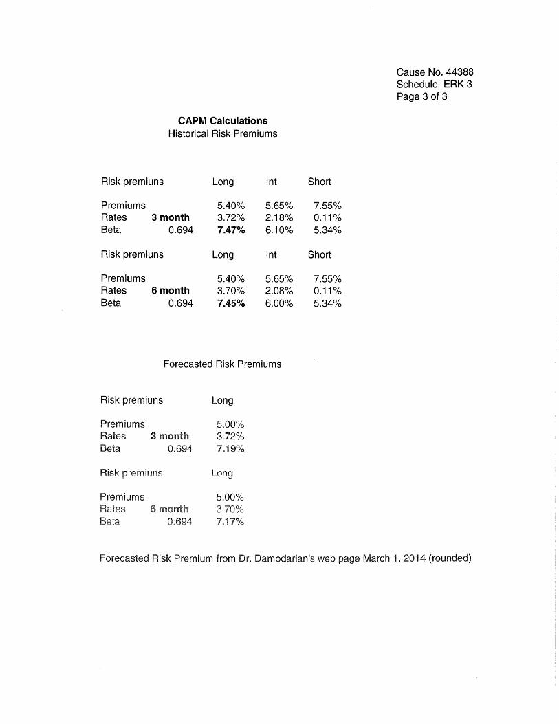
CAPM Calculations Historical Risk Premiums

Risk premiuns Long Int

Premiums 5.40% 5.650/0 Rates 3 month 3.72% 2.180/0 Beta 0.694 7.470/0 6.10%

Risk premiuns Long Int

Premiums 5.40% 5.65% Rates 6 month 3.70% 2.08% Beta 0.694 7.45% 6.00%

Forecasted Risk Premiums

Risk premiuns Long

Premiums Rates Beta

3 month 0.694

Risk premiuns

Premiums

5.00% 3.72% 7.19%

Long

7.1

Short

7.550/0 0.11% 5.34%

Short

7.55% 0.110/0 5.34%

Cause No. 44388 Schedule ERK 3 Page 3 of 3

Forecasted Risk Premium from Dr. Oamodarian's web page March 1, 4 (rounded)

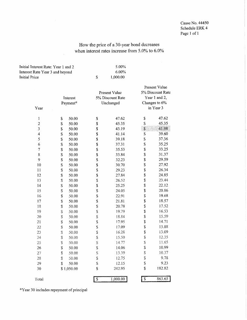
Cause No. 44450 Schedule ERK 4 Page I of 1

How the price of a 30-year bond decreases when interest rates increase from 5.0% to 6.0%

Initial Interest Rate: Year 1 and 2 5.00%

Interest Rate Year 3 and beyond 6.00% Initial Price $ 1,000.00

Present Value

Present Value 5% Discount Rate

Interest 5% Discount Rate Year 1 and 2,

Payment* Unchanged Changes to 6%

Year in Year 3

$ 50.00 $ 47.62 $ 47.62

2 $ 50.00 $ 45.35 $ 45.35

3 $ 50.00 $ 43.19 4 $ 50.00 $ 41.14 $ 39.60

5 $ 50.00 $ 39.18 $ 37.36

6 $ 50.00 $ 37.31 $ 35.25

7 $ 50.00 $ 35.53 $ 33.25

8 $ 50.00 $ 33.84 $ 31.37

9 $ 50.00 $ 32.23 $ 29.59

10 $ 50.00 $ 30.70 $ 27.92

11 $ 50.00 $ 29.23 $ 26.34

12 $ 50.00 $ 27.84 $ 24.85

13 $ 50.00 $ 26.52 $ 23.44

14 $ 50.00 $ 25.25 $ 22.12

15 $ 50.00 $ 24.05 $ 20.86

16 $ 50.00 $ 22.91 $ 19.68

17 $ 50.00 $ 21.81 $ 18.57

18 $ 50.00 $ 20.78 $ 17.52 HI '" 50.00 Ii' 19.79 $ 16.53 .17 cI) J!

20 $ 50.00 $ 18.84 $ 1';; ';;0 .LV • ..J/

21 $ 50.00 $ 17.95 $ 14.71

22 $ 50.00 $ 17.09 $ 13.88

23 '" 50.00 $ 16.28 $ l3.09 ..)j

24 $ 50.00 $ 15.50 $ 12.35

25 '" 50.00 $ $ L}}

26 $ 50.00 $ 14.06 $ 10.99

27 $ 50.00 <t' "I) 13.39 $ 10.37

28 d' 50.00 $ 12.75 $ 9.78 cI)

29 $ 50.00 $ 12.15 $ 9.23

30 $ 1,050.00 $ 242.95 $ 182.82

Total I $ 1,000.00 I [$ 863.65 I

*Year 30 includes repayment of principal

Flow Chart

Illustrat ing Pauline Ahern's Cost of Equity Analyses

Before adjusting for Company Specific Risks and Efficenty

I

Ibbotson Equity Risk Premium

5.60"-'

(BetoO.70)

~

,.-- -Predictive Risk Premium

Model (PRPM)

11.77%

S!!dul.:!PI :.! )

Beta Adjusted Equity Risk Pre mium

4.52%

Schedule 6, page 8

I

_ 1

Risk Premium Adjusted Marke t Approach

9.86%

Aver.~e

Equity ~isk Premium

4.61%

"-j Schedule 6, page 7

"Ib=on~ity=' 1 Premium B .. ed on

. PRPM

Lt 9. 26i&

(8eI3 0.70) J

r Equity Risk Premium Value Une Summa",

and Index

Lt ~ - -- (Beta 0.70)

Petitioner's Unadjusted Cost of Equity

10.15%

'-t Schedule 1, pages 2 -3

CAPM / ECAPM

9.80

Market Risk Premium DCf

11.23%

Schedule 8, pa~ 5

". - - - 1 ~ '"',.,' ''"-Predictive Risk Premium Arithimetic Me.n-I Model I Income Returns

10. 36~& 6.s5~'

S'::dU::': P'~ J Schedule 7, pace 2

Average of Historlc.1 and PRPM Equity Risk

Premium

4.71J'~

Schedule 6, page 11

,. - --'­

\

Ibbotson Equity lIisk Premium

~ (Beta 0.70)

Historic.1 Equity Risk J Forecasted Equity Risk 1 Premium Bnsed on Premium

PRPM 4.16";

5.24%

J ~

Estimat ed Costs of Equity are enlarged and bolded

Risk Premiums are in italics and underlined

Results based on Predictive Risk Premium M odel (PRPM™) are outlined in red/ dashed

...L ___

Comparable Risk Non-Price Regulated

Companies

10.50% '-I Schedule8~

Risk Premium Model

10.47%

Forecasted Equity Risk Premium

4.5~

Schedule 8, page 8

,. Ibbo:on ~ity rusk Equity Risk Premium Premium Based on Value Une Summa",

PRPM and Index

9.25"

...!,Bet,:!70J_ J

Value Une 3 to 5 Year MartetAppreciation

Potential

Cause No. 44450 Schedule ERK 5 Page 1 of l

CAPM/ECAPM

9.80%

Market Risk Premium

7.41"

Schedule 8, Page 9

Schedul~ 7, page 2 - --

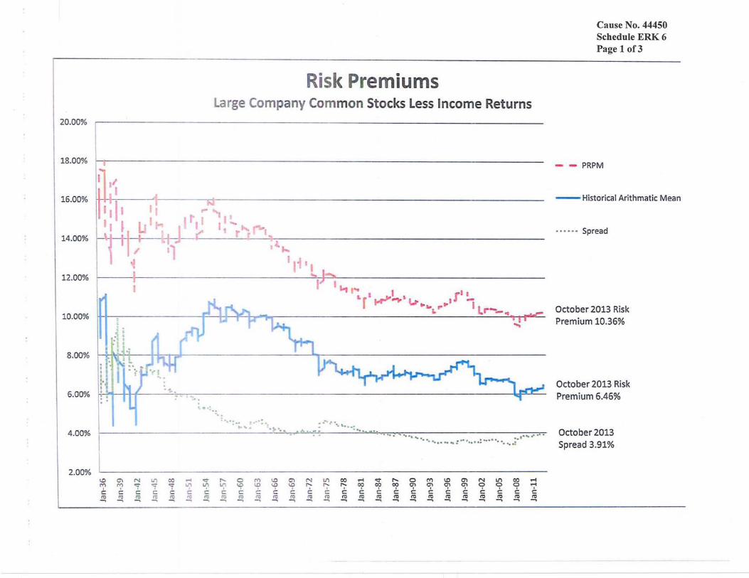
20.00%

18.00%

16.00%

14.00<70

12.00%

10.00%

8.00%

6.00%

4 .00%

2.00% l.O (j) ('oJ IJ) 0::) .-! ro M <::I" <::I" q- t.t)

C: C C: C C C ro ro ro ft! ro ft! ...... ...... ...... --. --. --.

·sk emiums Large Company Common Stocks Less Income Returns

... "r l

' .. " .. , ..... : .... . , ..

:: . .... J' ' " ~' . _.: .~._ , ....

-::I" r--. 0 ro l.O CI"I N t1"I 0::) M <::t Lfl I.J"I l.O 1.O l.O \.0 f'. r;- f'. 0::) co C C: C C: I C C C I ,.... C t: t: m ro ro ro ro ro ro ro ro I'D ro .... ...... ...... ...... ...... ...... ...... --. ...... ...... ......

I ..,. I" -..... ,.... I

l r __ ..

&.

"'"

" ...... " "''Pa,.. _ ..... ,. -.......... : .... " .... ,..... ,. .. , ....... .: a.. .. • .... ,..t·

"- 0 ro l.O CI"I ('oJ I.f'I 0::) .-! co O'l CI"I 0) 0) 0 0 0 .-I

C C: . C: C C I C I .- C t: I'D I'D ro I'D I'D ro ro ro ro ...... ...... ...... --. ...... ...... ...... ...... ......

Cause No. 44450 Schedule ERK 6 Page 1 of3

- - PRPM

- Historical Arithmatic Mean

...... Spread

October 2013 Risk Premium 10.36%

October 2013 Risk Premium 6.46%

October 2013 Spread 3.91%

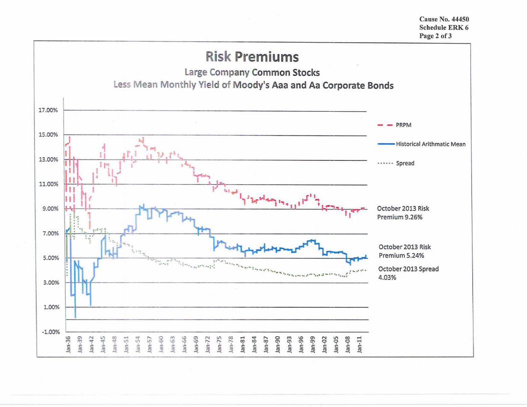
17.00%

15.00%

13.00%

11.00%

9.00%

7.00% ':

5.00%

3.00%

1.00%

-1.00% t.O 0'\ N U1 00 ~ ro <:j" '1 <::t

C: C: I

c: c: c: ro ro ro ro ~ -.. -.. ....., .....,

• s emlums large Company Common Stocks

Cause No. 44450 Schedule ERK 6 Page 2 of3

ess Mean Monthly Yield of Moody's Aaa and Aa Corporate Bonds

... ...... . .... .. .,.. if'" • _ .. -: .. to . ..

'" ct.r a• ..... ·"i-:

,.... -.;t I'- 0 m ~ 0'\ N If) 00 1.1) 1..)"1, I.f) \.0 \.0 ~ \.0 I'- I'- " I I I I C

, C:

, C: C: c: C r- C c:

co ~ ~ ~ ~ ro ro ~ ro ro -. ....,. ....,. ....,. ....,.

I, J

..... ·"' .. 1

"" ,-.. z -.... - , t o ....... _ . . ..... ... " I' .. ..... ..:r _ .' ". " •••• .......... ..

£">

,.... <::t " 0 m U) 0'\ N t.n co ,.... co 00 00 0"1 (j) 0"1 0"1 0 0 0 .-t , I C: C: C: I C: C: C: C:

, c c: c c: co co co co ~ ro ro co co co ro -.. -, ...., -, -. ...., -.. ....,. ...., -..

.~.'-' ~.--.. -..... ~-.-'---' ~--' .. ------- .' .. -.~. --.'. ---_.-,

- - PRPM

- Historical Arithmatic Mean

" ••••• Spread

October 2013 Risk Premium 9.26%

October 2013 Risk Premium 5.24%

October 2013 Spread 4.03%

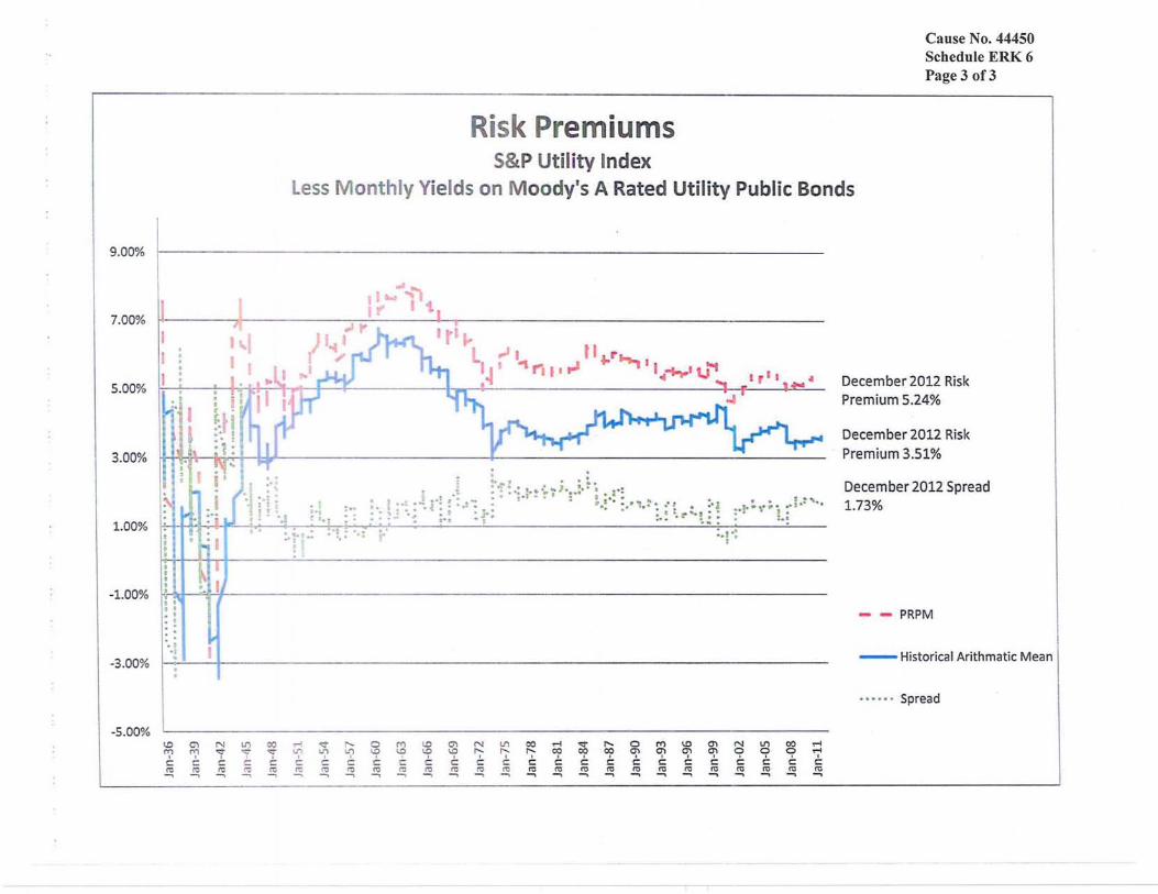
9.00<}o

7.00%

5.00%

3.00%

1.00%

-1.00%

-3.00%

-5.00% t.O (j) N l/') 00 "';l (Y') 1- ~ <:T

c C t: C co co ro co co -.. -, -, -, -,

USK Premiums S&P Utility Index

Cause No. 44450 Schedule ERK 6 Page 3 of3

Less Monthly Yields on Moody's A Rated Utility Public Bonds

M <::t L';'t ~ c ~ ro -. ....,

:.. ~, .. . :. .. .- ; .~~.:; ... :' ,: ; .. ,,: .. ... ,.: ~ . Ht ·~.r! : :.:': .. ~ . ~. : f'.f- : .• , .. !,. ~.~ • :' l i.!\'~ ' •. ~ .~ " •• ... J to.! ; .. : :i~; . :.! :.tt-·! :: :. f.:

- .! :.1-:

r--. 0 M !.O (j) N LO 00 .-I <::t I'- 0 M \.0 0'\ N LO 00 M

LQ \.0 !.O \.0 !.O I'- I'- r-- 00 00 00 0'\ 0'\ 0'\ 0'\ 0 a a '7 c C: t: C C C C C C: C C C C C: C C: C: C t:

~ ~ ro co ro co ro !!; ro ro co ro ~ ro co ro co co ro ..., ...., ...., ...., -, ...., ...., ...., -, -, -, ...., -, -, -,

December 2012 Risk Premium 5.24%

December 2012 Risk Premium 3.51%

December 2012 Spread 1.73%

- - PRPM

- Historical Arithmatic Mean

...... Spread

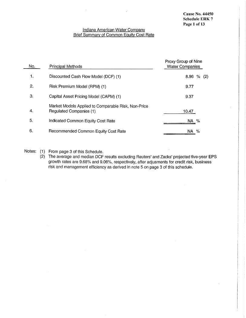
No.

1.

2.

3.

4.

5.

6.

Indiana American Water Company Brief Summary of Common Equity Cost Rate

Principal Methods

Discounted Cash Flow Model (DCF) (1)

Risk Premium Model (RPM) (1)

Capital Asset Pricing Model (CAPM) (1)

Market Models Applied to Comparable Risk, Non-Price Regulated Companies (1)

Indicated Common Equity Cost Rate

Recommended Common Equity Cost Rate

Cause No. 44450 Schedule ERK 7 Page 1 of13

Proxy Group of Nine Water Companies

8.96 % (2)

9.77

9.37

10.47

NA %

NA %

Notes: (1) From page 3 of this Schedule. (2) The average and median DCF results excluding Reuters' and Zacks' projected five-year EPS

growth rates are 9.68% and 9.08%, respectively, after adjusments for credit risk, business risk and management efficiency as derived in note 5 on page 3 of this schedule,

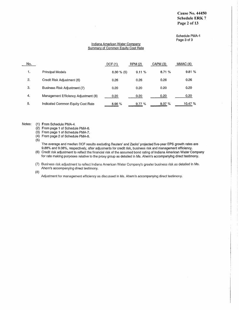
No.

1.

2.

3.

4.

5.

Indiana American Water Company Summary of Common Equity Cost Rate

DCF (i) RPM (21

Principal Models 8.30 % (5) 9.11 %

Credit Risk Adjustment (6) 0.26 0.26

Business Risk Adjustment (7) 0.20 0.20

Management Efficiency Adjustment (8) 0.20 0.20

Indicated Common Equity Cost Rate 8.96 % 9.77 %

CAPM {3}

8.71 %

0.26

0.20

0.20

9.37%

Cause No. 44450 Schedule ERK 7 Page 2 of13

Schedule PMA-1 Page30f3

MMAC (4}

9.81 %

0.26

0.20

0.20

10.47 %

Notes: (1) From Schedule PMA-4. (2) From page 1 of Schedule PMA-6. (3) From page 1 of Schedule PMA-7. (4) From page 2 of Schedule PMA-8. (5)

The average and median DCF results excluding Reuters' and Zacks' projected five-year EPS growth rates are 9.88% and 9.08%, respectively, after adjusments for credit risk, business risk and management efficiency.

(6) Credit risk adjustment to reflect the financial risk of the assumed bond rating of Indiana American Water Company for rate making purposes relative to the proxy group as detailed in Ms. Ahern's accompanying direct testimony.

(7) Business risk adjustment to reflect Indiana American Water Company's greater business risk as detailed in Ms. Ahern's accompanying direct testimony.

(8) Adjustment for management efficiency as discussed in Ms. Ahern's accompanying direct testimony.

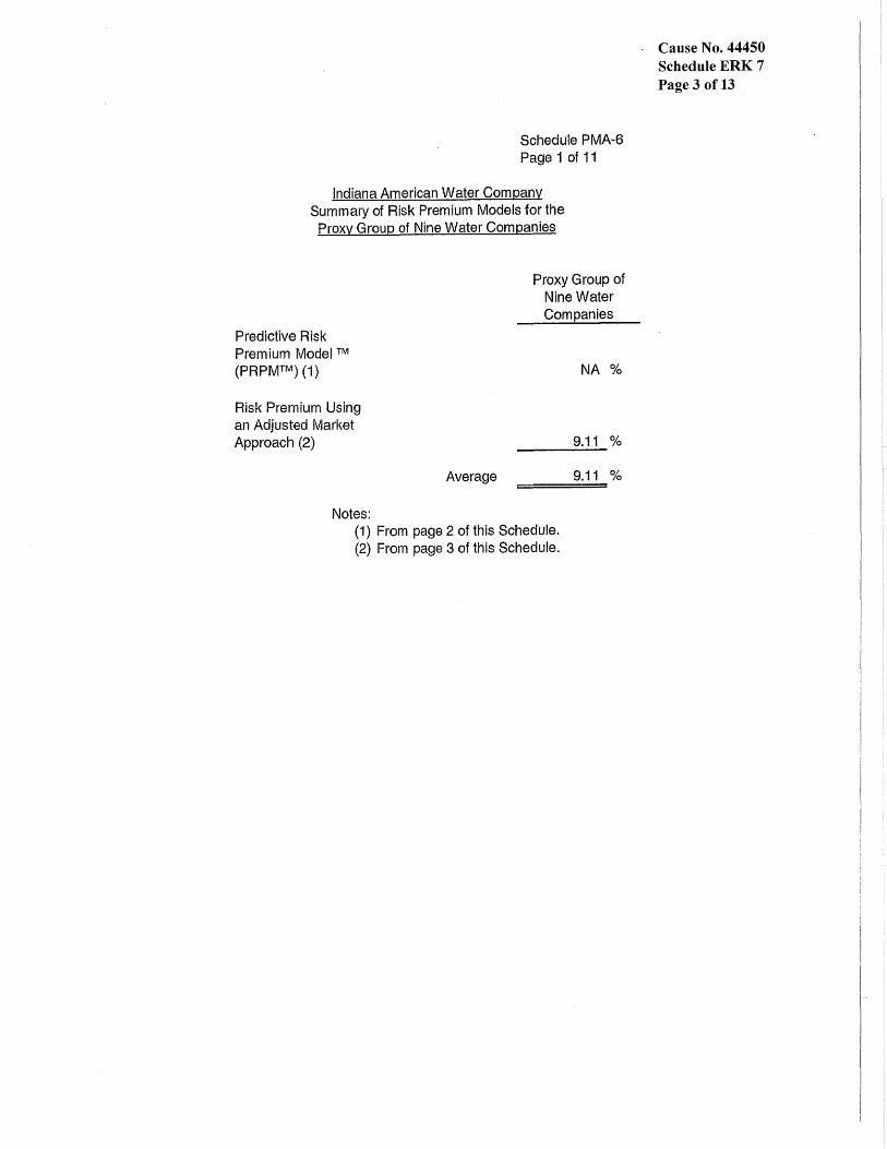
Schedule PMA-6 Page 1 of 11

Indiana American Water Company Summary of Risk Premium Models ,for the

Proxy Group of Nine Water Companies

Predictive Risk Premium Model ™ (PRPMTM) (1)

Risk Premium Using an Adjusted Market Approach (2)

Notes:

Average

Proxy Group of Nine Water Companies

NA %

9.11 %

9.11 %

(1) From page 2 of this Schedule. (2) From page 3 of this Schedule.

Cause No. 44450 Schedule ERK 7 Page 3 of13

Line No.

1.

2.

3.

4.

5.

6.

7.

Indiana American Water Company Indicated Common Equity Cost Rate

Through Use of a Risk Premium Model Using an Adjusted Total Market Approach

Prospective Yield on Aaa Rated Corporate Bonds (1)

Adjustment to Reflect Yield Spread Between Aaa Rated Corporate Bonds and A Rated Public Utility Bonds

Adjusted Prospective Yield on A Rated Public Utility Bonds

Adjustment to Reflect Bond Rating Difference of Proxy Group

Adjusted Prospective Bond Yield

Equity Risk Premium (5)

Risk Premium Derived Common Equity Cost Rate

Cause No. 44450 Schedule ERK 7 Page 4 of13

Schedule PMA-6 Page 3 of 11

Proxy Group of Nine Water Companies

5.11 %

0.17 (2)

5.28 %

(0.04) (3)

5.25 %

Notes: (1) Six quarter average consensus forecast ending with Q1 of 2015 averaged with the 2015-2019 and 2020-2023 consensus forecast of Moody's Aaa Rated Corporate bonds from Blue Chip Financial Forecasts (see pages 9 and "10 of this Schedule).

(2) The average yield spread of A rated public utility bonds over Aaa rated corporate bonds of 0.17% from page 6 of this Schedule.

(3) Adjustment to reflect the A1/A2 Moody's bond rating of the proxy group of nine water companies as shown on page 4 of this Schedule. The 4 basis point adjustment is derived by taking 1/6 of the spread between Aa2 and A2 Public Utility Bonds (1/6 * 0.21 % = 0.04%).

(4) From page 7 of this Schedule.

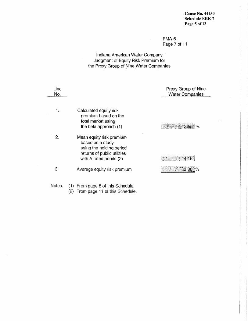
Cause No. 44450 Schedule ERK 7 Page 5 of13

PMA-6 Page 7 of 11

Indiana American Water Company Judgment of Equity Risk Premium for

the Proxy Group of Nine Water Companies

Line No.

1. Calculated equity risk premium based on the total market using the beta approach (1)

2. Mean equity risk premium based on a study using the holding period returns of public utilities with A rated bonds (2)

Average equity risk premium

Notes: (1) From page 8 of this Schedule. (2) From page 11 of this Schedule.

Proxy Group of Nine Water Companies

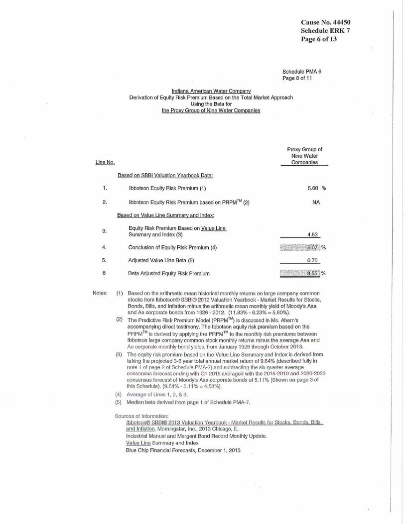
1.

2.

3.

Indiana American Water Companv

Cause No. 44450 Schedule ERK 7 Page 6 of13

Schedule PMA 6 Page 8 of 11

Derivation of Equity Risk Premium Based on the Total Market Approach Using the Beta for

the Proxy Group of Nine Water Companies

Based on SBBI Valuation Yearbook Data:

Ibbotson Equity Risk Premium (1)

Ibbotson Equity Risk Premium based on PRPM™ (2)

Based on Value Line Summarv and Index:

Equity Risk Premium Based on Value Line Summary and Index (3)

Proxy Group of Nine Water Companies

5.60 %

NA

4.53

4. Conclusion of Equity Risk Premium (4)

5. Adjusted Value Line Beta (5) 0.70

6 Beta Adjusted Equity Risk Premium

Notes: (1) Based on the arithmetic mean historical monthly returns on large company common stocks from Ibbotson® SBBI® 201 2 Valuation Yearbook · Market Results for Stocks, Bonds, Bills, and Inflation minus the arithmetic mean monthly yield of Moody's Aaa and Aa corporate bonds from 1926 · 201 2. (11.83% · 6.23% = 5.60%) .

(2) The Predictive Risk Premium Model (PRPM TM) is discussed in Ms. Ahern 's accompanying direct testimony. The Ibbotson equity risk premium based on the

PRPM™ is derived by applying the PRPM™ to the monthly risk premiums between Ibbotson large company common stock monthly returns minus the average Aaa and Aa corporate monthly bond yields, from January 1926 through October 2013.

(3) The equity risk prem ium based on the Value Line Summary and Index is derived from tal<ing the projected 3-5 year total annual market retu rn of 9.64% (described fu lly In note '1 of page 2 of Schedule PMA· 7) and subtracting the six quarter average consensus forecast ending with 01 2015 averaged with the 2015·201 9 and 2020·2023 consensus forecast of Moody's Aaa corporate bonds of 5.11 % (Shown on page 3 of this Schedule) . (9.64% · 5.11 % == 4.53%).

(4) Average of Lines 1,2, & 3.

(5) Median beta derived from page 1 of Schedule PMA-7.

Sources of Information: Ibbotson® SBBI® 2013 Valuation Yearbook - Market Results for Stocks. Sands. Bills. and Inflation, Morningstar, Inc., 2013 Ch icago, IL. Industrial Manual and Mergent Bond Record Monthly Update. Va lue Line Summary and Index

Blue Chip Financial Forecasts, December 1, 201 3

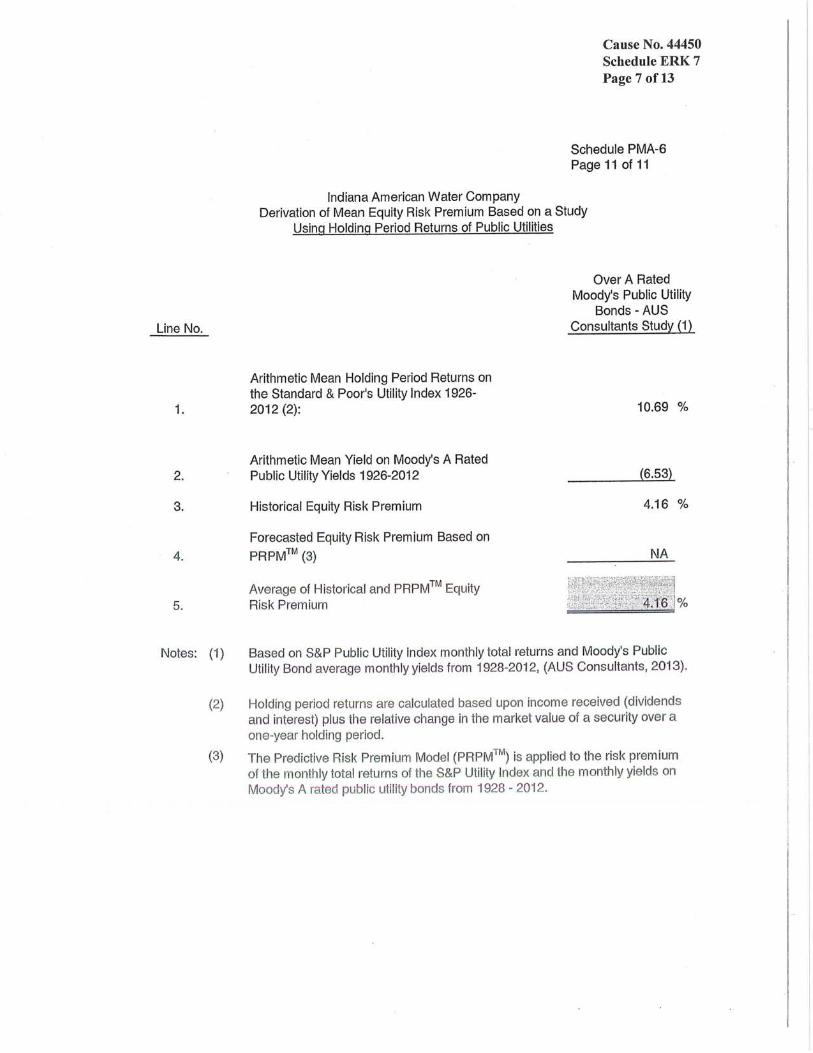
Line No.

1.

2.

3.

4.

Indiana American Water Company

Cause No. 44450 Schedule ERK 7 Page 7of13

Schedule PMA-6 Page 11 of 11

Derivation of Mean Equity Risk Premium Based on a Study Using Holding Period Returns of Public Utilities

Arithmetic Mean Holding Period Returns on the Standard & Poor's Utility Index 1926-2012 (2):

Arithmetic Mean Yield on Moody's A Rated Public Utility Yields 1926-2012

Historical Equity Risk Premium

Forecasted Equity Risk Premium Based on

PRPM™ (3)

Average of Historical and PRPM™ Equity

Over A Rated Moody's Public Utility

Bonds - AUS Consultants Study (1)

10.69 %

(6.53)

4.16 %

NA

5. Risk Premium

Notes: (1) Based on S&P Public Utility Index monthly total returns and Moody's Public Utility Bond average monthly yields from 1928-2012, (AUS Consultants, 2013).

(2) Holding period returns are calculated based upon income received (dividends and interest) plus the relative change in the market value of a security over a one~year holding period.

(3) The Predictive Risk Premium Model (PRPM™) is appl ied to the risk premium of the monthly total returns of the S&P Utility Index and the monthly yields on Moody's A rated public utility bonds from 1928 - 2012.

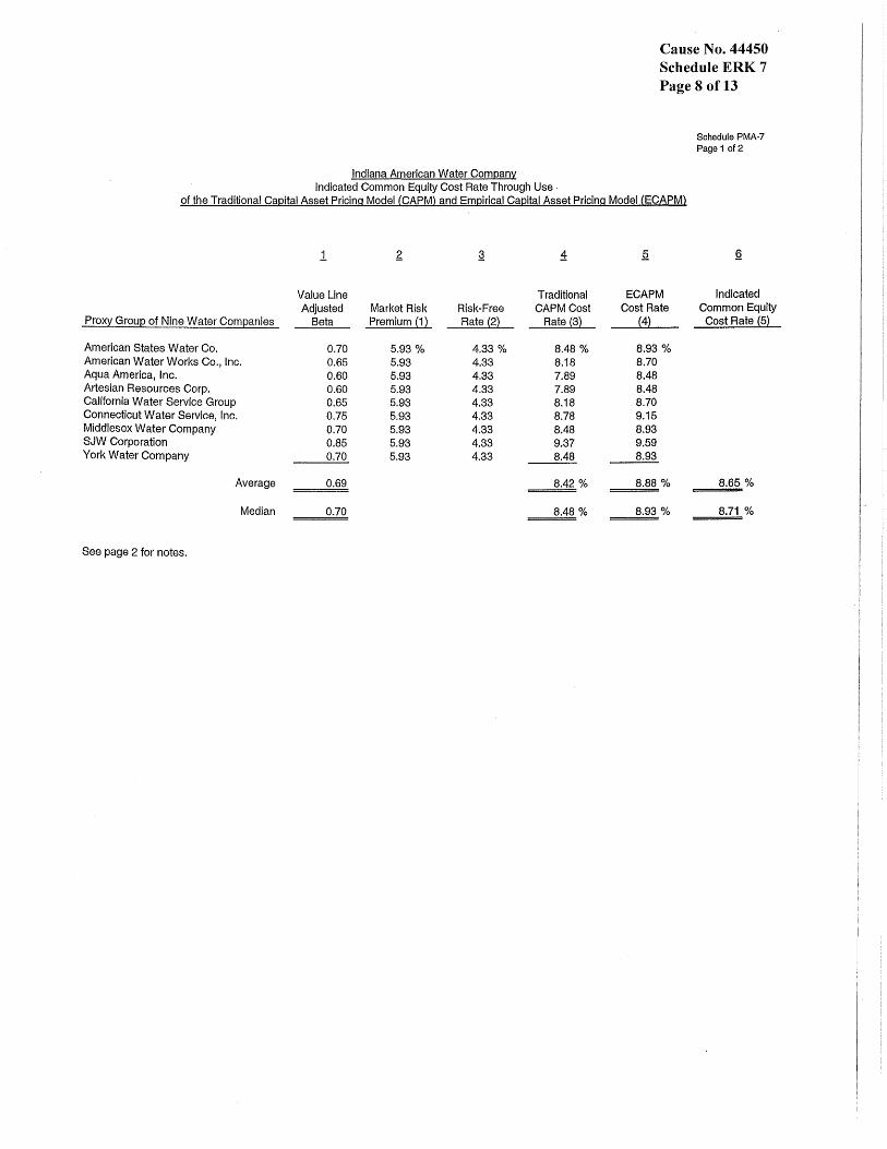
Indiana American Water Company Indicated Common Equity Cost Rate Through Use·

Cause No. 44450 Schedule ERK 7 Page 8 of13

Schedule PMA-7 Page 1 of2

of the Traditional Capital Asset Pricing Model (CAPM) and Empirical Capital Asset Pricing Model (ECAPM)

1 g ~ 1 .Q .§

Value Line Traditional ECAPM Indicated Adjusted Market Risk Risk-Free CAPM Cost Cost Rate Common Equity

Prox~ GroUI2 of Nine Water Coml2anies Beta Premium {1} Rate (2) Rate {3} (4) Cost Rate {5}

American States Water Co. 0.70 5.93% 4.33 % 8.48 % 8.93 % American Water Works Co., Inc. 0.65 5.93 4.33 8.18 8.70 Aqua America, Inc. 0.60 5.93 4.33 7.89 8.48 Artesian Resources Corp. 0.60 5.93 4.33 7.89 8.48 California Water Service Group 0.65 5.93 4.33 8.18 8.70 Connecticut Water Service, Inc. 0.75 5.93 4.33 8.78 9.15 Middlesex Water Company 0.70 5.93 4.33 8.48 8.93 SJW Corporation 0.85 5.93 4.33 9.37 9.59 York Water Company 0.70 5.93 4.33 8.48 8.93

Average 0.69 8.42 % 8.88 % 8.65 %

Median 0.70 8.48 % 8.93 % 8.71 %

See page 2 for notes.

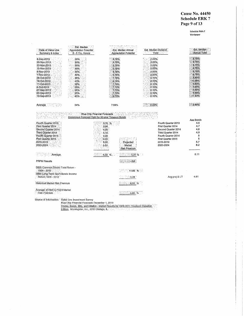
·'~ Date. ofValueUne ' .. " summ~ry & Index'

~~pe~~2d1.3· .. ·29~Nov~2013.· .•

:j~J~6~~i~g, ' : . a.·N()Y~201$

.@~~i~£Jj~'.':·'~i~ '.' '18'9ot~gO:1 $;-.

~if~'~l~'~ ..... . 1 ~~.$EiP·2b~ S . '.

AYElrag~

: : )::8t. Nledif:Jn, ",. ;·.Appieq.l~tiol'l pot~niial

3· 5Yrs.:Hence ..

.30%' .. • .. : :30%":" ..

>.3()o/.Q········. ., :.3(J%.'·

:,(~~~:: '. ">35%"

:.AO%.··'·' ·:.:~3~o/.,· . "':"$50/(>' "<'~9%;"

. " i.:~~~~:'~~ .,·:i 34% 7,59%

" .. "':':':- . .', ~'.;": ·:~j3:(.~~·'.·~~.tp_~ F'i~:anbi~l F~·~e9~i~t.s·: :,:}:.~.~> ... -.. ~:-:", ;:". ".'-." ... Consensus ForecastYieldfor 30.yeari"reasuiY .Bonds·

·i=()~~h:9~~~e~:26I(:\

:~~b~~4~{rt~~16~t; Jhir9:o.~~rte(2QH·.::: :f9lilth:qYa.ri~ij!o1~·:i:' 'Firet Qtiaite~ 2015: <

:~~~~~,~~&~:~'~";'r .• ';:,

PRPM Results

$BBIC6riimonS!ock$'Toiai Reiurn­::1926 ~ 2012>:;'" :SaBiF(;JnQ"TermGq~iBOnds Income ' .. Retuiii 1926':'2012 .

BlstQik;at~arket Risk premium

/'w~r~g~9!H)~t~f ~pr()j'd Market Rlskprernium', ..

!;'ir,{X~~~li§ :i :: Risk Premium

Cause No. 44450 Schedule ERK 7 Page 9 of13

!~. ~ ::. . :;?~(j9!o.! '2,00%:

:::>2.0Qo/~] ,>:,,2;00"(0;

2.00%.

·····Mt1!, >l';;~iii

'':':;:2.:·10ci&~

Fourth Quarter 2013 First Quarter 2014 Second Quarter 2014 Third Quarter 2014 Fourth Quarter 2014 First Quarter 2015 2015-2019 2020-2024

Avg proj & LT

Schedule PMA-7 Workpaper

Aaa Bonds 4.6 4.7 4.8 4.9

5 5

5.7 6.2

5.11

4.81

Source ofinfdirnaiion: . V~II~e Line Investment 8U/vey Blue Chip Financial Forecasts December 1, 2013 Stdck~:Bdhds~··Bills~~iidjhfiailoh:Mari(erResultsf6f.1926·201'1 Yeirbo6kV~I~'atiori'" Editidn'lVIDrnlngsiar~lnc:, 2612 Chicago, IL .... ." .. .... ' ....

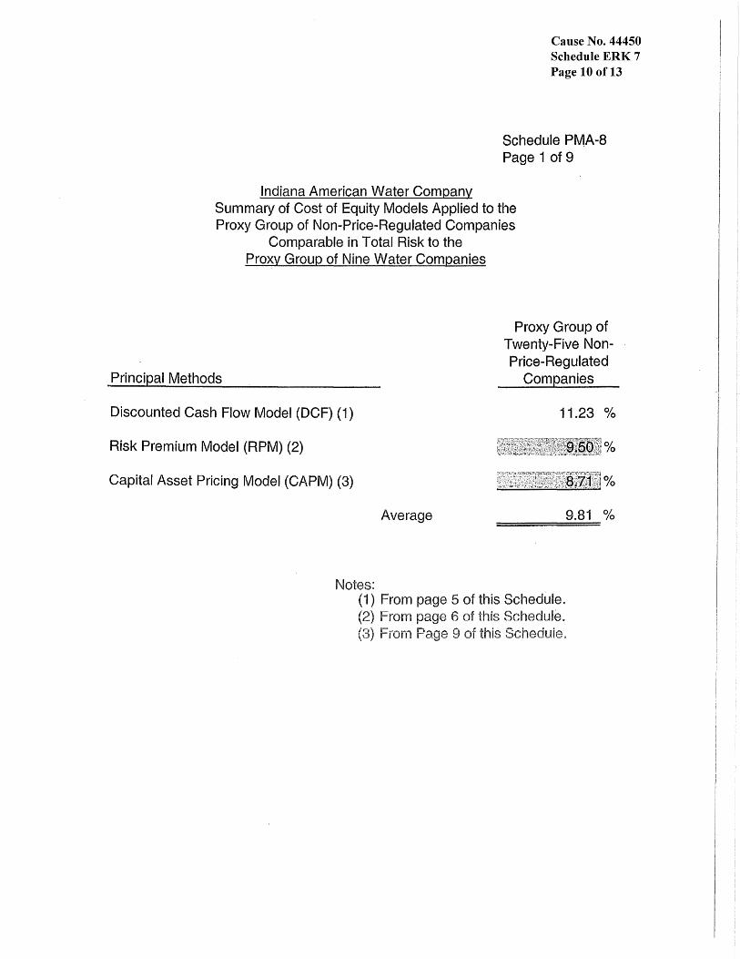
Cause No. 44450 Schedule ERK 7 Page 10 of13

Schedule PMA-8 Page 1 of 9

Indiana American Water Company Summary of Cost of Equity Models Applied to the Proxy Group of Non-Price-Regulated Companies

Comparable in Total Risk to the Proxy Group of Nine Water Companies

Principal Methods

Discounted Cash Flow Model (DCF) (1)

Risk Premium Model (RPM) (2)

Capital Asset Pricing Model (CAPM) (3)

Notes:

Average

Proxy Group of Twenty-Five Non­Price-Regulated

Companies

11.23 0/0

9.81 %

(1) From page 5 of this Schedule. (2) From page 6 of this Schedule.

9

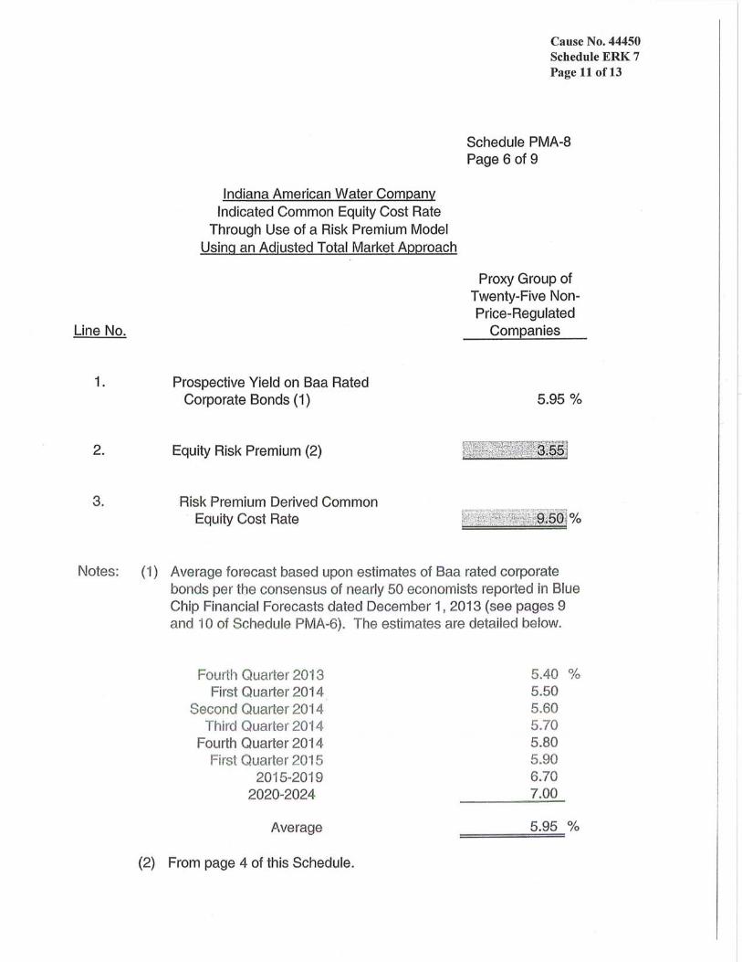
Line No.

1 .

Indiana American Water Company Indicated Common Equity Cost Rate

Through Use of a Risk Premium Model Using an Adjusted Total Market Approach

Prospective Yield on Baa Rated Corporate Bonds (1)

Cause No. 44450 Schedule ERK 7 Page 11 of13

Schedule PMA-8 Page 6 of 9

Proxy Group of Twenty-Five Non­Price-Regulated

Companies

5.95 0/0

2. Equity Risk Premium (2)

3. Risk Premium Derived Common . Equity Cost Rate

Notes: (1 ) Average forecast based upon estimates of Baa rated corporate bonds per the consensus of nearly 50 economists reported in Blue Chip Financial Forecasts dated December 1, 2013 (see pages 9 and 10 of Schedule PMA-6). The estimates are detailed below.

Fourth Quarter 2013 5.40 0/0 First Quarter 2014 5.50

Second Quarter 2014 5.60 Third Quarter 2014 5.70

Fourth Quarter 2014 5.80 First Quarter 2015 5.90

2015-2019 6.70 2020-2024 7.00

Average 5.95 0/0

(2) From page 4 of this Schedule.

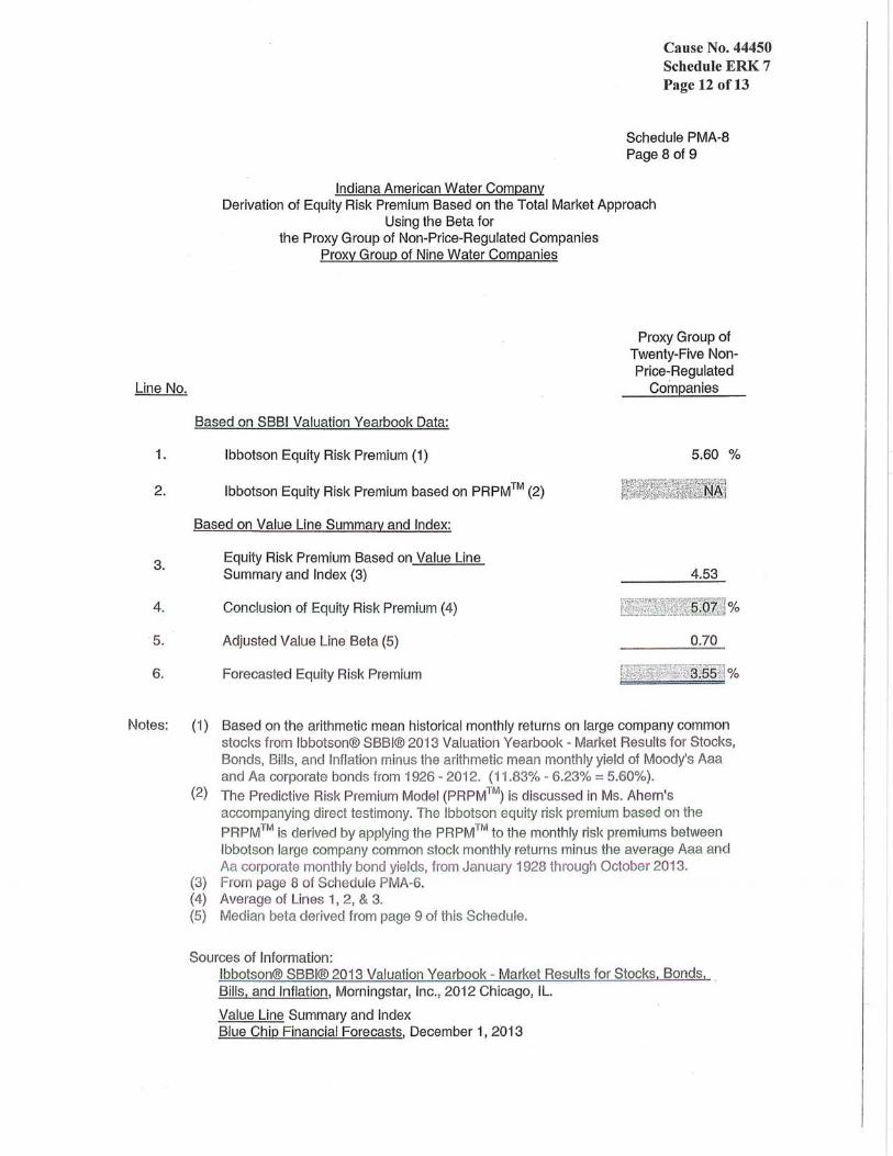
Line No.

1.

Indiana American Water Company

Cause No. 44450 Schedule ERK 7 Page 12 of13

Schedule PMA-8 Page 8 of 9

Derivation of Equity Risk Premium Based on the Total Market Approach Using the Beta for

the Proxy Group of Non-Price-Regulated Companies Proxy Group of Nine Water Companies

Based on SBBI Valuation Yearbook Data:

Ibbotson Equity Risk Premium (1)

Proxy Group of Twenty-Five Non­Price-Regulated

Companies

5.60 %

2. Ibbotson Equity Risk Premium based on PRPM ™ (2)

3.

4.

5.

6.

Based on Value Line Summary and Index:

Equity Risk Premium Based on Value Line Summary and Index (3)

Conclusion of Equity Risk Premium (4)

Adjusted Value Line Beta (5)

Forecasted Equity Risk Premium

4.53

%

0.70

Notes: (1) Based on the arithmetic mean historical monthly return s on large company common stocks from Ibbotson® SBBI® 2013 Valuation Yearbook - Market Results for Stocks, Bonds, Bills , and Inflation minus the arithmetic mean monthly yield of Moody1s Aaa and Aa corporate bonds from 1926 - 201 2. (11.83% - 6.23% = 5.60%).

(2) The Predict ive Risk Premium Model (PRPM TM) is discussed in Ms. Ahern1s accompanying direct testimony. The Ibbotson equity risk premium based on the

PRPM ™ is derived by applying the PRPM ™ to the monthly risk premiums between Ibbotson large company common stock monthly returns minus the average Aaa and Aa corporate monthiy bond yields, from January 1928 through October 2013.

(3) From page 8 of Schedule PMA-6. (4) Average of Lines 1, 2, & 3. (5) Median beta derived from page 9 of this Schedule.

Sources of Information: Ibbotson® SBBI® 2013 Valuation Yearbook - Market Results for Stocks, Bonds, Bills, and Inflation, Morn ingstar, Inc. , 2012 Chicago, IL.

Value Line Summary and Index Blue Chip Financial Forecasts, December 1, 2013

Indiana American Water Company

Cause No. 44450 Schedule ERK 7 Page 13 of13

Schedule PMA·8 Page90f9

Traditional CAPM and ECAPM Results for the Proxy Group of Non-Price-Regulated Companies Comparable in Total Risk to the Proxy Group of Nine Water Companies

Proxy Group of Twenty-Five Value Line Traditional Indicated Non-Priee-Regulated Adjusted Marl<et Risk Risk-Free CAPM Cost ECAPM Cost Common Equity Companies Beta Premium (1) Rate (2) Rate (3) Rate (4) Cost Rate (5)

Gallagher (Arthur J.) 0.75 5.93 % 4.33 % 8.78 % 9.15 % AutoZone Inc. 0.60 5.93 4.33 7.89 8.48 Baxter Inti Inc. 0.75 5.93 4.33 8.78 9.15 Bristol-Myers Squibb 0.70 5.93 4.33 8.48 8.93 Brown & Brown 0.75 5.93 4.33 8.78 9.15 CenturyLink Inc. 0.75 5.93 4.33 8.78 9.15 DaVita HealthCare 0.70 5.93 4.33 8.48 8.93 Haemonetlcs Corp. 0.65 5.93 4.33 8.18 8.70 J&J Snaek Foods 0.70 5.93 4.33 8.48 8.93 Kroger Co. 0.60 5.93 4.33 7.89 8.48 Lancaster Colony 0.70 5.93 4.33 8.48 8.93 Mercury General 0.65 5.93 4.33 8.18 8.70 Markel Corp. 0.75 5.93 4.33 8.78 9.15 Annaly Capital Mgmt. 0.60 5.93 4.33 7.89 8.48 Northwest Bancshares 0.70 5.93 4.33 8.48 8.93 Owens & Minor 0.75 5.93 4.33 8.78 9.15 Raytheon Co. 0.75 5.93 4.33 8.78 9.15 Sherwin-Williams 0.65 5.93 4.33 8.18 8.70 Smucker (J.M.) 0.65 5.93 4.33 8.18 8.70 Silgan Holdings 0.70 5.93 4.33 8.48 8.93 Stericycle Inc. 0.65 5.93 4.33 8.18 8.70 Molson Coors Brewing 0.65 5.93 4.33 8.18 8.70 Waste Connections 0.75 5.93 4.33 8.78 9.15 Weis Markets 0.65 5.93 4.33 8.18 8.70 Berkley (W.R.) 0.65 5.93 4.33 8.18 8.70

Average 0.69 8.41 % 8.87 % 8.64 %

Median 0.70 8.48 % 8.93 % 8.71 %

Notes: (1) From Schedule PMA-7, page 2, note 1. (2) From Schedule PMA-7, page 2, note 2. (3) Derived from the model shown on Schedule PMA-7, page 2, note 3. (4) Derived from the model shown on Schedule PMA-7, page 2, note 4. (5) Average of CAPM and ECAPM cost rates.

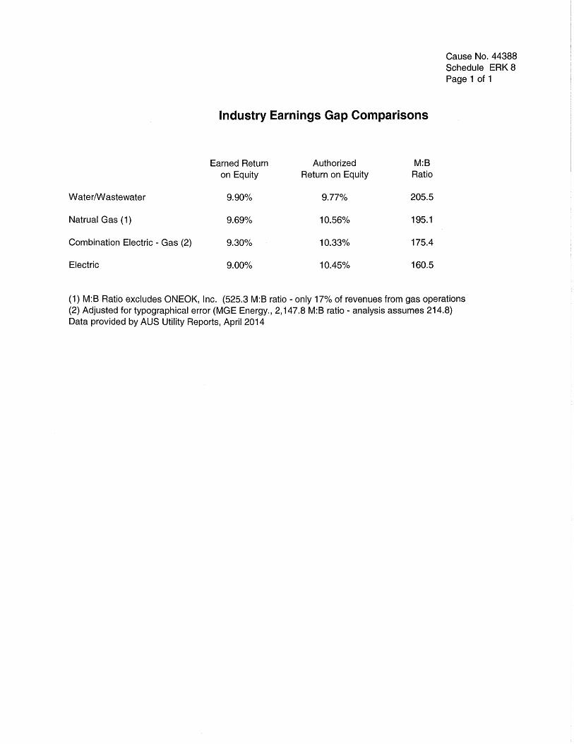
Water/W astewater

Natrual Gas (1)

Combination Electric - Gas (2)

Electric

Industry Earnings Gap Comparisons

Earned Return Authorized M:B on Equity Return on Equity Ratio

9.90% 9.77% 205.5

9.69% 10.56% 195.1

9.30% 10.33% 175.4

9.00% 10.45% 160.5

Cause No. 44388 Schedule ERK 8 Page 1 of 1

(1) M:B Ratio excludes ONEOK, Inc. (525.3 M:B ratio - only 17% of revenues from gas operations (2) Adjusted for typographical error (MGE Energy., 2,147.8 M:B ratio - analysis assumes 214.8) Data provided by AUS Utility Reports, April 2014

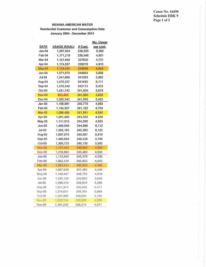
Cause No. 44450 Schedule ERK 9 Page 1 of3

INDIANA AMERICAN WATER

Residential Customer and Consumption Data

January 2004 - December 2013

Mo. Usage

DATE USAGE {KGAL} # Cust. percust.

Jan-04 1,267,824 236,525 5,360

Feb-04 1,171,218 236,546 4,951

Mar-04 1,121,945 237630 4,721

Apr-04 1,174,557 239216 4,910

May-04 1,115,445 239948 4,649

Jun-04 1,371,070 240693 5,696

Jul-04 1,341,666 241203 5,562

Aug-04 1,475,337 241435 6,111

Sep-04 1,315,349 242113 5,433

Oct-04 1,421,742 241,834 5,879

Nov-04 923A24 241,093 3,830

Oec-04 1,302,342 241,055 5,403

Jan-05 1,196,081 240,775 4,968

Feb-OS 1,134,327 241,122 4,704

Mar-OS 1,098,499 241,561 4,548

Apr-05 1,201,460 243,322 4,938

May-OS 1,111,813 244,200 4,553

Jun-OS 1,496,849 244,896 6,112

Jul-05 1,502,193 245,360 6,122

Aug-OS 1,697,675 245,687 6,910

Sep-OS 1,406,058 246,439 5,706

Oct-OS 1,369,733 246,138 5,565

Nov-OS 1,127.403 245,600 4.590

Dec-OS 1,216,965 245,469 4 ,958

Jan-06 1,112,945 245,378 4,536

Feb-06 1,092,310 245,853 4,443

Mar-06 1,082,413 246,569 4 ,390

Apr-06 1,097.848 247,480 4,436

May-06 1,148,447 248.793 4 ,61 6

Jun-06 ",420,158 249,660 5,688

Jul-06 1,299,4 '19 249.910 5,200

Aug-06 '1,621,974 250,650 6,471

Sep-06 1,274,651 250.70 1 5,'084

Oct-D6 1,297,009 249,824 5,192

Nov-06 -1,020,744 24 ,036 ,099

Dec-06 1,161,239 248,274 4,677

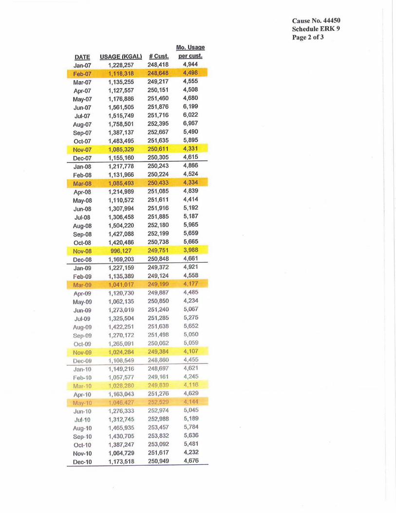
Cause No. 44450 Schedule ERK 9 Page 2 of3

Mo. Usage

DATE USAGE {KGAL} # Cust. percust.

Jan-07 1,228,257 248,418 4,944

Feb-07 1,118,318 248,648 4,498

Mar-07 1,135,255 249,217 4,555

Apr-07 1,127,557 250,151 4,508

May-07 1,176,886 251,460 4,680

Jun-07 1,561,505 251,876 6,199

Jul-07 1,515,749 251,716 6,022

Aug-07 1}58,501 252,395 6,967

Sep-07 1,387,137 252,667 5,490

Oct-07 1,483,495 251,635 5,895

Nov-07 1,085,329 250,611 4 ,331

Dec-07 1,155,160 250,305 4,615

Jan-08 1,217,778 250,243 4,866

Feb-08 1,131,966 250,224 4,524

Mar-08 1.085,493 250.433 4.334

Apr-08 1,214,989 251,085 4,839

May-08 1,110,572 251,611 4,414

Jun-08 1,307,994 251 ,916 5,192

Jul-08 1,306,458 251 ,885 5,187

Aug-08 1,504,220 252,180 5,965

Sep-08 1,427,088 252,199 5,659

Oct-08 1,420,486 250}38 5,665

Nov-08 996.127 249,751 3,988

Dec-08 1,169,203 250,848 4,661

Jan-09 1,227,159 249,372 4,921

Feb-09 1,135,389 249,124 4,558

Mar-09 1,041 .017 249.199 4.177

Apr-09 1,120,730 249,887 4,48

May-09 1.062,135 250,850 4,234

Jun-09 1,273,019 251 ,240 5,067

Jul-09 1,325,504 251 ,285 5,275

Aug-09 1,422,251 251,638 5,652

Sep-09 1,270,172 251,498 5,050

Oct-09 1,265,091 250,062 5,059

Nov-09 1,024,284 249,384 4,107

Dec-09 '1.108,549 248,860 4,455

.Jan-10 1,149,216 248,697 4,621

Feb-10 1,057,577 249,161 4,245

Mar-10 1.028.2 0 ?4 .81Q 4,11~

Apr-10 1,163,043 251,276 4,629

Mav 10 1.046 <12r ~5 52 4.14

Jun-10 1,276,333 252,974 5,045

Jul-10 1,312,745 252,988 5, 189

Aug-i0 1,465,935 253,457 5,784

Sep-10 1,430}05 253,832 5,636

Oct-10 1,387,247 253,092 5,481

Nov-10 1,064,729 251,617 4.232

Dec-10 1,173,518 250,949 4,676

Cause No. 44450 Schedule ERK 9 Page 3 of3

Mo. Usage

DATE USAGE {KGAL} # Cust. percust.

Jan-11 1,102,203 250,640 4,398

Feb-11 1,041,970 250,868 4,153

Mar-11 1,029,570 251,098 4,100

Apr-11 1,077,702 251,977 4,277

May-11 1.017,368 252,681 4,026

Jun-11 1,254,736 253,493 4,950

JUI-11 1,280,440 253,655 5,048

Aug-11 1,543,000 254,120 6,072

Sep-11 1,362,615 253,850 5,368

Oct-11 1,193,261 252,670 4,723

Nov-11 982,929 251,721 3,905

Oec-11 1,060,582 251,493 4,217

Jan-12 1.086,465 251.309 4.323

Feb-12 1,049,893 251,538 4,174

Mar-12 990,147 252,287 3,925

Apr-12 1,066,849 253,452 4,209

May-12 1,042,345 254,668 4,093

Jun-12 1,567,322 256,955 6,100

JUI-12 1,635,769 256,926 6,367

Aug-12 1,633,877 257,276 6,351

Sep-12 1,216,820 256,965 4,735

Oct-12 1,156,348 255,659 4,523

Nov-12 1,008,544 255,021 3,955

Oec-12 1,058,072 255,268 4,145

Jan-13 1,049,887 255,181 4,114

Feb-13 1,036,960 255,753 4,055 lowest usage

Mar-13 1,008,132 256,137 3.936 2nd lowest usage

A r-13 1, 14 2 1 2 7 I 4

May-13 1,1 17,807 260,021 4,299

Jun-13 1,230,389 260,563 4,722

JUI-13 1,222,674 261,059 4,684

Aug-13 1,374,320 261,546 5,255

Sep-13 1,337,829 261,642 5,113

Oct-13 '1,223,383 260,228 4,701

Nov-13 1,034,808 259,359 3,990

ec-13 1,054,472 259,062 4,070